Mechanistic Pavement DesignA Road to Enhanced Understanding of Pavement Performance

Sigurdur ErlingssonDept. of Civil and Env. EngineeringUniversity of IcelandIceland&Dept. of Highway EngineeringVTISweden

Seminar on Pavement Design System and Pavement Performance ModelsReykjavik, 22.–23. March, 2007

Outline

• The Problem• Current Design Methods• Mechanistic-Empirical Design Methods• Important Factors Influencing Pavement Performance

– Traffic Loading– Material Characteristics– The Climatic Conditions and Seasonal Variation of Pavement Response

• Response Calculation and Distress Prediction• Validation

– Accelerated Testing of Pavement Structure

• Conclusion

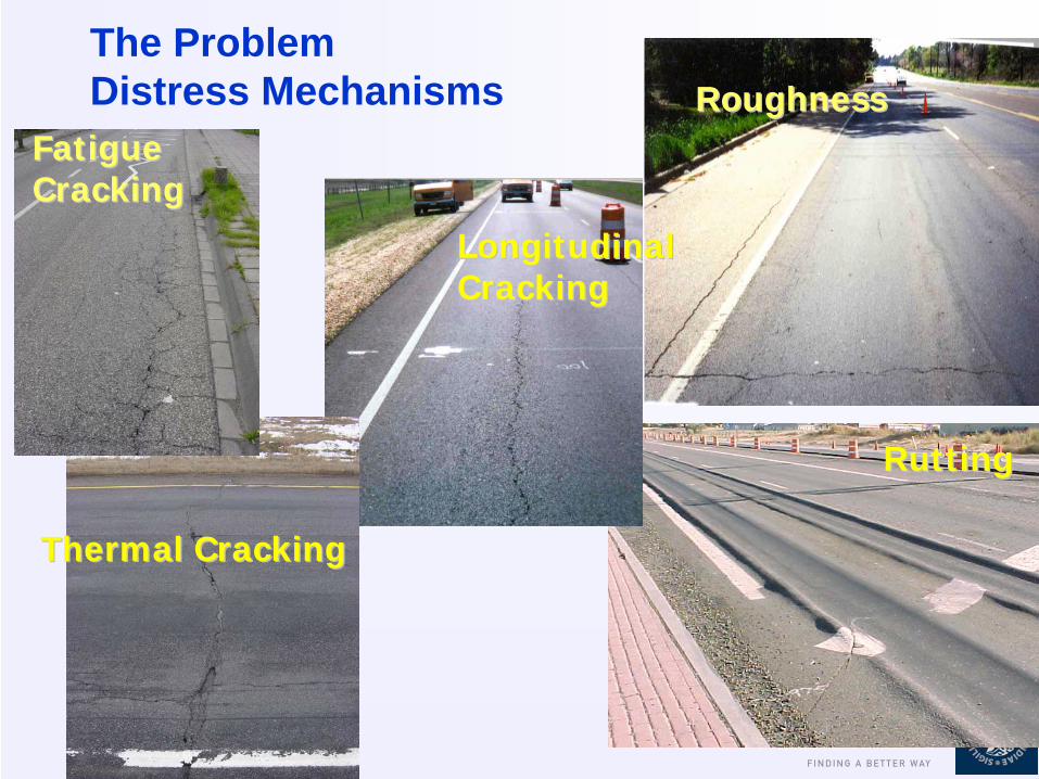
The Problem Distress Mechanisms

Longitudinal Longitudinal CrackingCracking

RoughnessRoughness

Thermal CrackingThermal Cracking

RuttingRutting

Fatigue Fatigue CrackingCracking

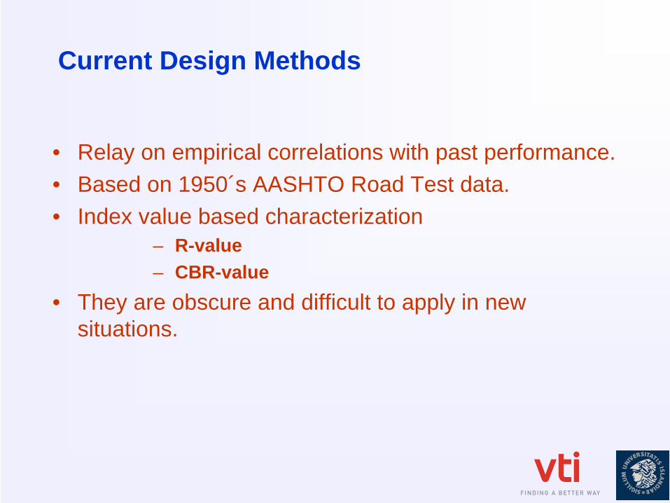
Current Design Methods

• Relay on empirical correlations with past performance.• Based on 1950´s AASHTO Road Test data.• Index value based characterization

– R-value– CBR-value

• They are obscure and difficult to apply in new situations.

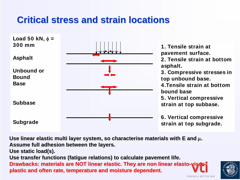
Load 50 kN, φ

= 300 mm

Asphalt

Unbound or BoundBase

Subbase

Subgrade

1. Tensile strain at pavement surface.2. Tensile strain at bottom asphalt.3. Compressive stresses in top unbound base.4.Tensile strain at bottom bound base5. Vertical compressive strain at top subbase.

6. Vertical compressive strain at top subgrade.

CriticalCritical stress and stress and strainstrain locationslocations

UseUse linearlinear elasticelastic multimulti layerlayer system, system, soso characterisecharacterise materialsmaterials withwith E and E and μμ..AssumeAssume full full adhesionadhesion betweenbetween the the layerslayers..UseUse static static loadload(s).(s).UseUse transfer transfer functionsfunctions ((fatiguefatigue relations) to relations) to calculatecalculate pavementpavement lifelife..Drawbacks: Drawbacks: materialsmaterials are NOT are NOT linearlinear elasticelastic. . TheyThey are non are non linearlinear elastoelasto--viscovisco-- plasticplastic and and oftenoften raterate, , temperaturetemperature and and moisturemoisture dependentdependent..

Mechanistic-Empirical Design

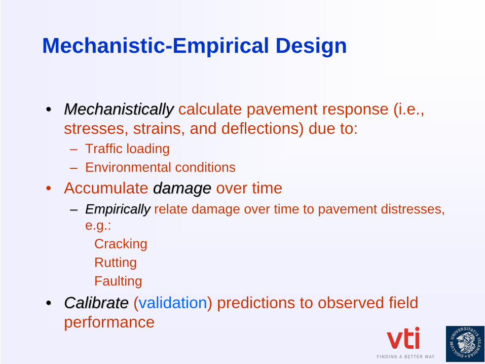
•• MechanisticallyMechanistically calculate pavement response (i.e., stresses, strains, and deflections) due to:– Traffic loading– Environmental conditions

• Accumulate damagedamage over time–– EmpiricallyEmpirically relate damage over time to pavement distresses,

e.g.:CrackingRuttingFaulting

•• CalibrateCalibrate (validation) predictions to observed field performance

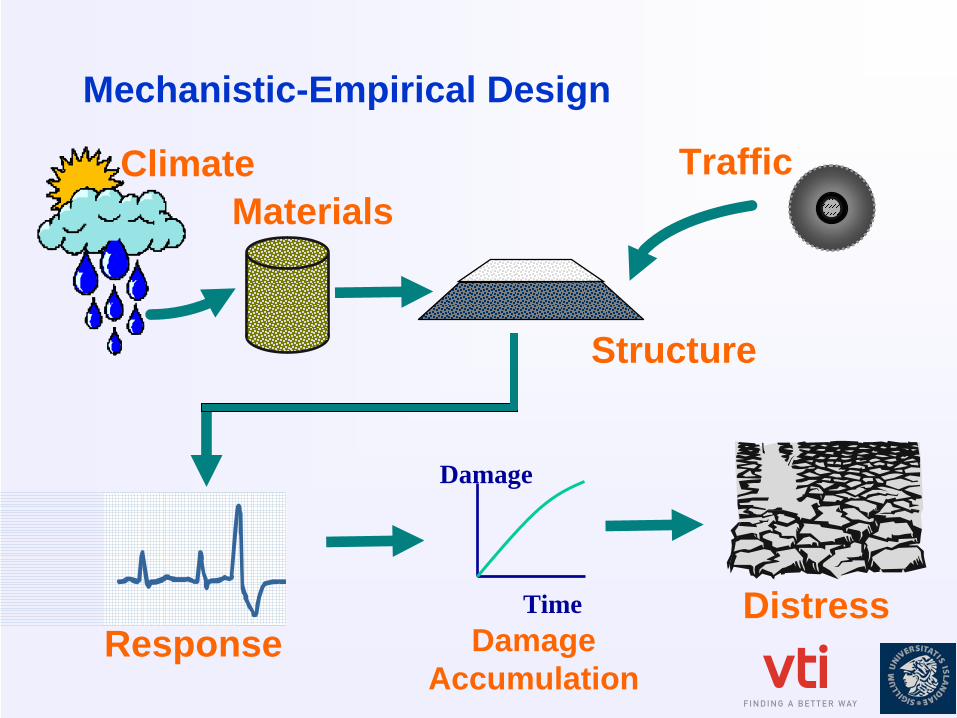
Mechanistic-Empirical Design

Climate TrafficMaterials

Structure

DistressResponse

Time

Damage

Damage Accumulation

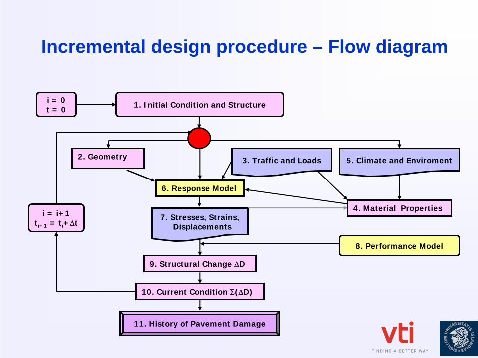
Incremental design procedure – Flow diagram

1. Initial Condition and Structure

2. Geometry

4. Material Properties

6. Response Model

10. Current Condition Σ(ΔD)

5. Climate and Enviroment

7. Stresses, Strains,Displacements

9. Structural Change ΔD

8. Performance Model

i = 0t = 0

11. History of Pavement Damage

i = i+1ti+1 = ti +Δt

3. Traffic and Loads

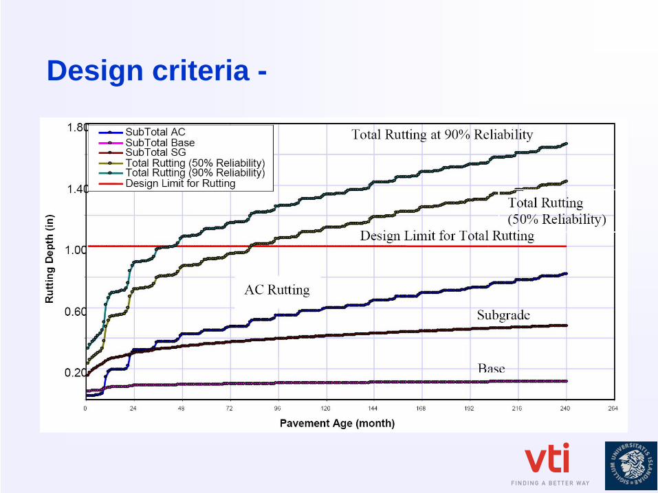
Design criteria -

Factors Influencing Performance and Distress Development

• Traffic Loading• Material Characteristics• Climatic Conditions and Seasonal Variation of Material

Properties

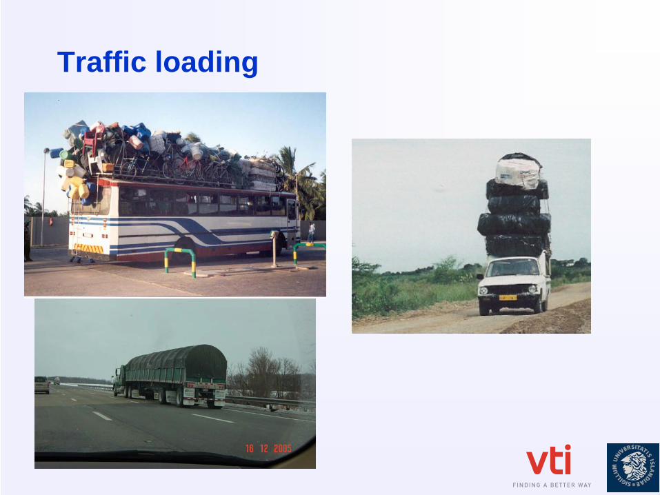
Traffic loading

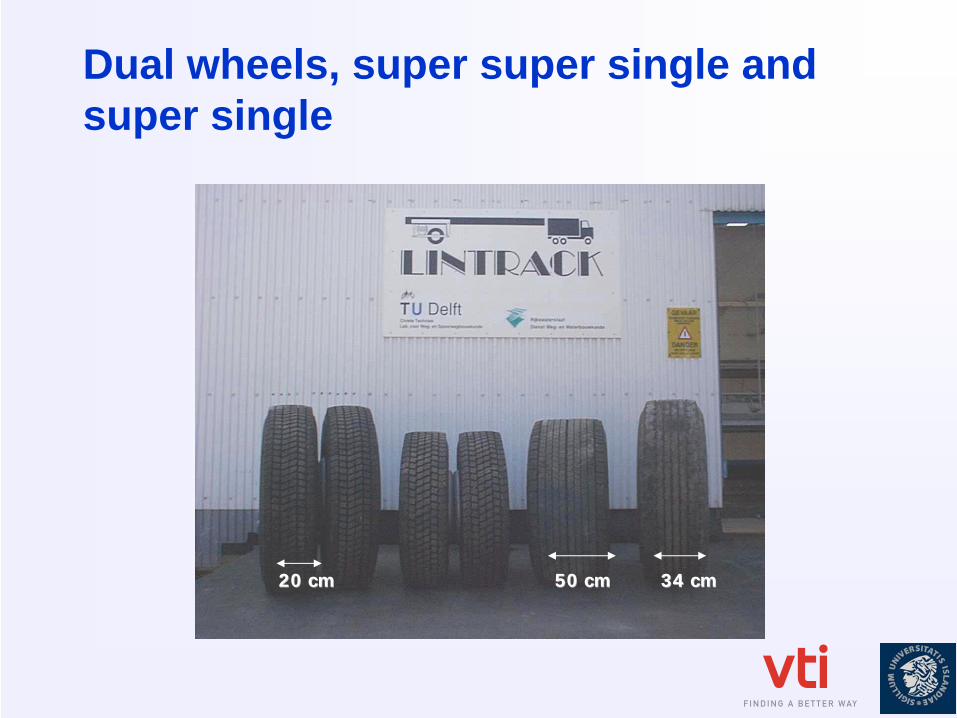
Dual wheels, super super single and super single

20 cm 50 cm 34 cm20 cm 50 cm 34 cm

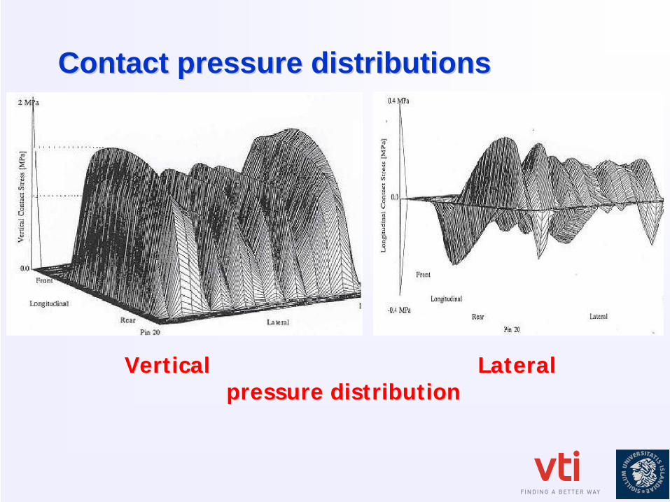
Contact Contact pressurepressure distributionsdistributions

Vertical LateralVertical Lateralpressure distributionpressure distribution

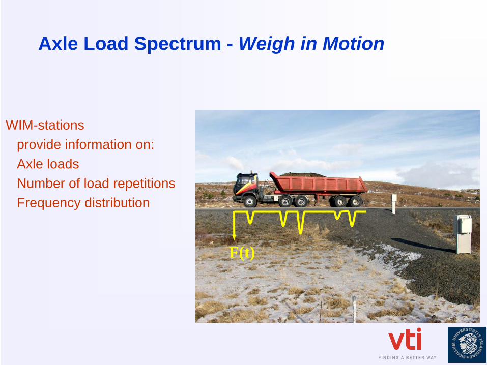
Axle Load Spectrum - Weigh in Motion

WIM-stationsprovide information on:Axle loadsNumber of load repetitionsFrequency distribution

F(t)

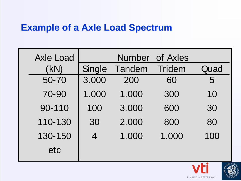
Example of a Axle Load SpectrumExample of a Axle Load Spectrum

Axle Load(kN)

Single

NumberTandem

of AxlesTridem

Quad

50-70 3.000 200 60 5 70-90 1.000 1.000 300 10 90-110 100 3.000 600 30 110-130 30 2.000 800 80 130-150 4 1.000 1.000 100

etc

Material Properties - Dynamic testing

Layer Test method Property

Asphalt Concrete Triaxial Testing Indirect Tension TestUniaxial CompressionBending Test

Stiffness, perm def.Stiffness, Fatigue CreepFatigue

Bitumin.stab. Base Course

Triaxial TestingIndirect Tension TestUniaxial Compression

StiffnessStiffness, Fatigue Creep

Unbound granular materials

Triaxial Testing Stiffness, Permanent Deformation Behaviour

Dynamic testing simulates field conditions better than static testing, therefore a better correlation is expected with field performance.

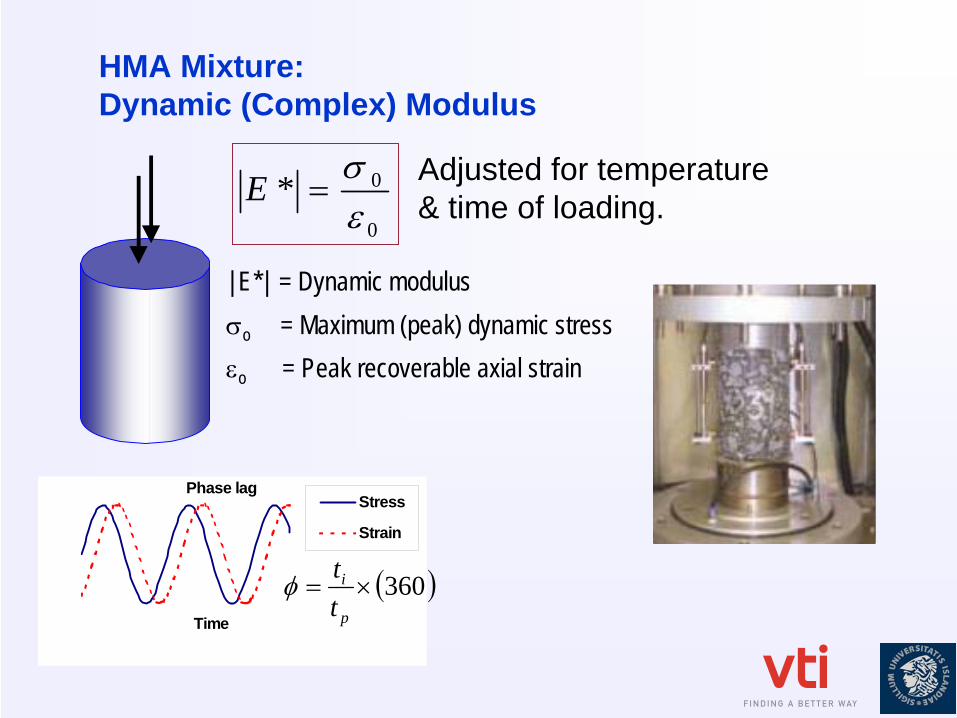
HMA Mixture: Dynamic (Complex) Modulus

0

0*εσ

=E

Stress

Strain

Phase lag

Time

| E*| = Dynamic modulusσo = Maximum (peak) dynamic stressεo = Peak recoverable axial strain

( )360×=p

i

ttφ

Adjusted for temperature & time of loading.

HMA - Material Properties Indirect Tension test

W

AC

Subbase

Subgrade

εx σy

Base course

Time

Loa

d

Time

Def

orm

atio

n

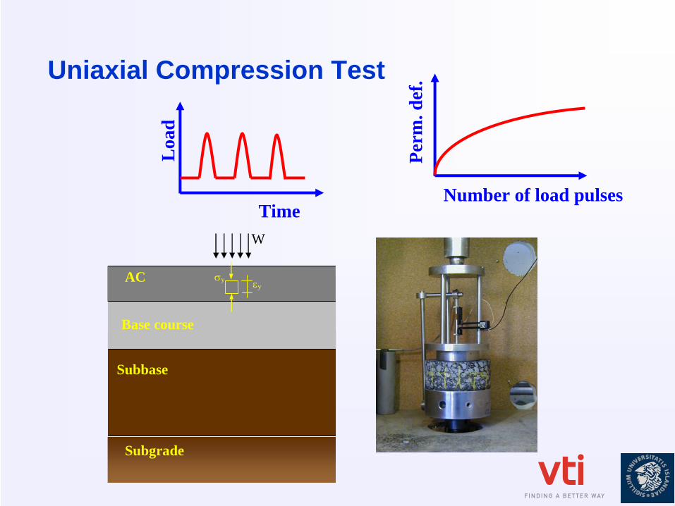
Uniaxial Compression Test

W

AC

Subbase

Subgrade

εy σy

Base course

Time

Loa

dNumber of load pulses

Perm

. def

.

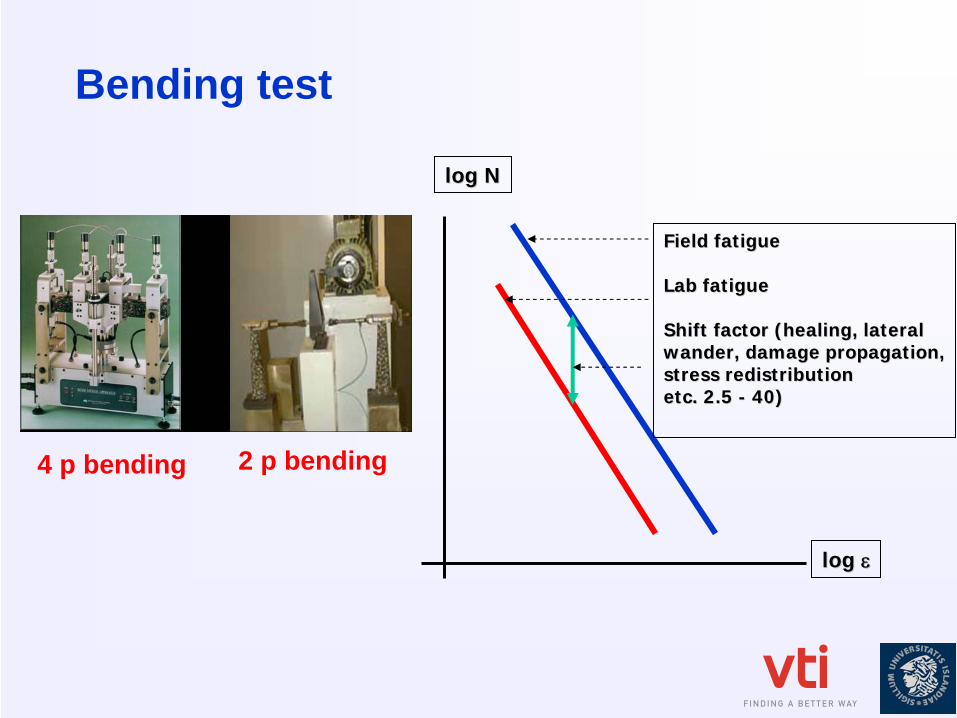
Bending test

4 p bending 2 p bending

log log εε

log Nlog N

Field Field fatiguefatigue

Lab Lab fatiguefatigue

Shift factor (Shift factor (healinghealing, , laterallateralwanderwander, , damagedamage propagationpropagation,,stress stress redistributionredistributionetc. 2.5 etc. 2.5 -- 40)40)

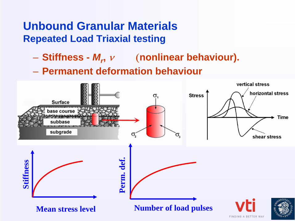
Unbound Granular Materials Repeated Load Triaxial testing

– Stiffness - Mr , ν

(nonlinear behaviour).– Permanent deformation behaviour

Number of load pulses

Perm

. def

.

Mean stress level

Stiff

ness

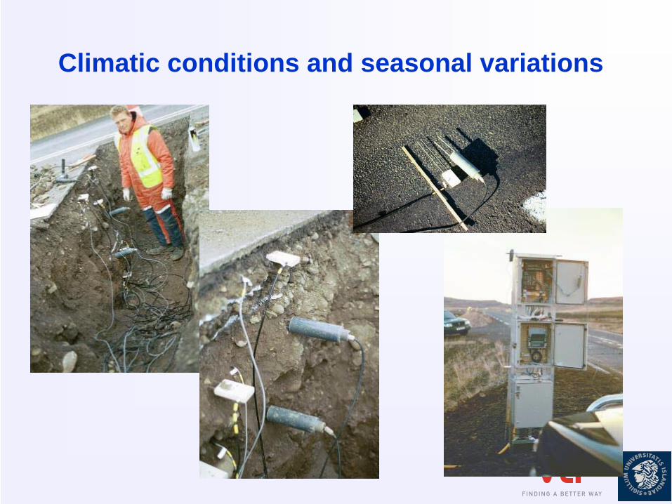
Climatic conditions and seasonal variations

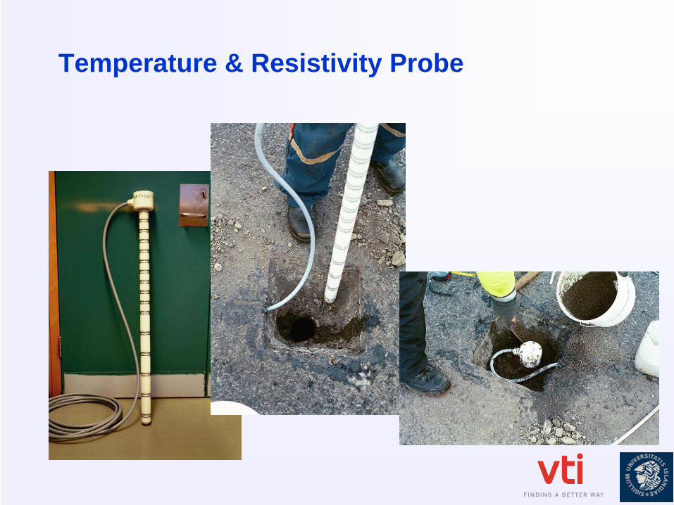
Temperature & Resistivity Probe

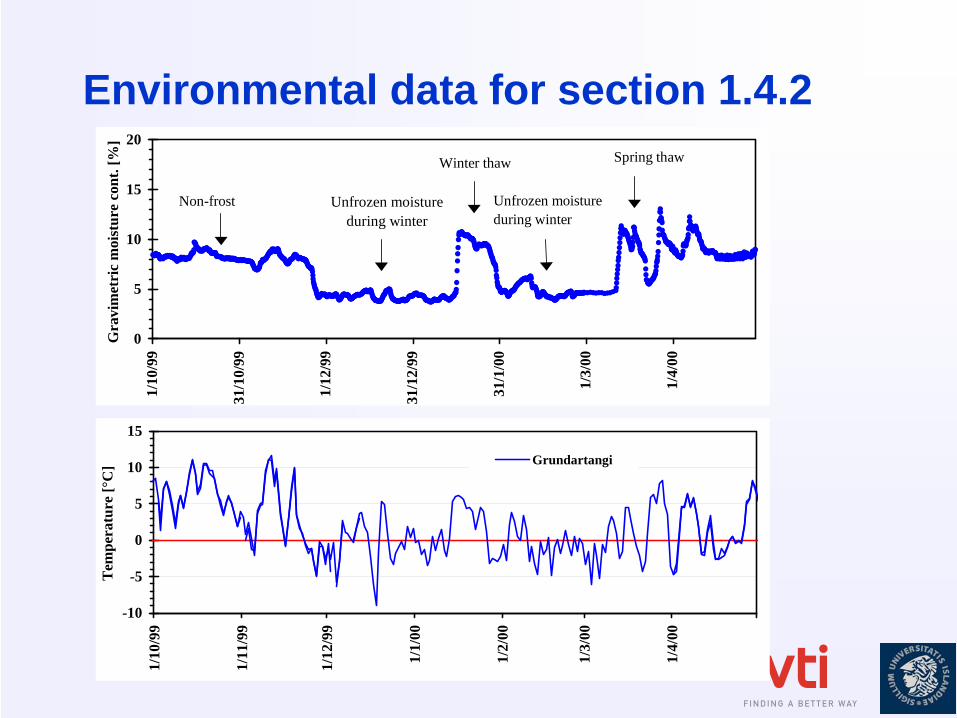
Environmental data for section 1.4.2

Unfrozen moistureduring winter

0

5

10

15

201/

10/9

9

31/1

0/99

1/12

/99

31/1

2/99

31/1

/00

1/3/

00

1/4/

00

Gra

vim

etri

c m

oist

ure

cont

. [%

]

Winter thaw

Unfrozen moistureduring winter

Spring thaw

Non-frost

-10

-5

0

5

10

15

1/10

/99

1/11

/99

1/12

/99

1/1/

00

1/2/

00

1/3/

00

1/4/

00

Tem

pera

ture

[°C

] Grundartangi

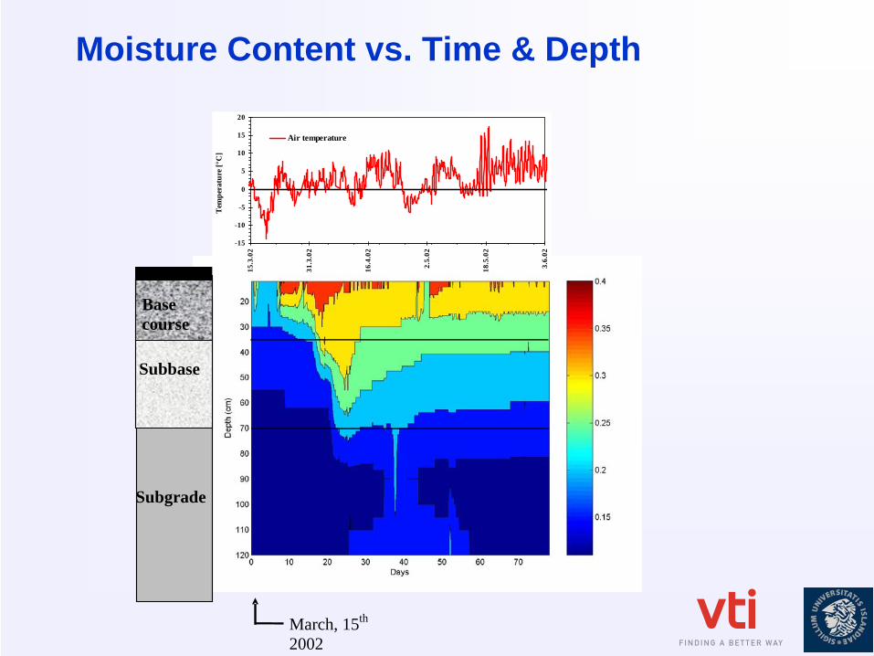
Moisture Content vs. Time & Depth

Subgrade

Subbase

Base course

March, 15th 2002

-15

-10

-5

0

5

10

15

20

15.3

.02

31.3

.02

16.4

.02

2.5.

02

18.5

.02

3.6.

02

Tem

pera

ture

[°C

]

Air temperature

Frost Resistivity Probe

Sensor 1, d = 5 cm Sensor 2, d = 10 cm

0

20

40

60

80

100

120

1 3 5 7 9 11 13 15 17 19 21 23

No. measurements

Rel

ativ

e co

nduc

tivity

[%

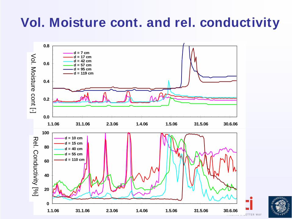
Vol. Moisture cont. and rel. conductivity

0.0

0.2

0.4

0.6

0.8

1.1.06 31.1.06 2.3.06 1.4.06 1.5.06 31.5.06 30.6.06

Vegr

aki [

-]

d = 7 cmd = 17 cmd = 42 cmd = 57 cmd = 95 cmd = 119 cm

0

20

40

60

80

100

1.1.06 31.1.06 2.3.06 1.4.06 1.5.06 31.5.06 30.6.06

Hlu

tfalls

leg

rafle

iðni

d = 10 cmd = 15 cmd = 40 cmd = 55 cmd = 110 cm

Vol. M

oisture cont [-]R

el. Conductivity [%

]

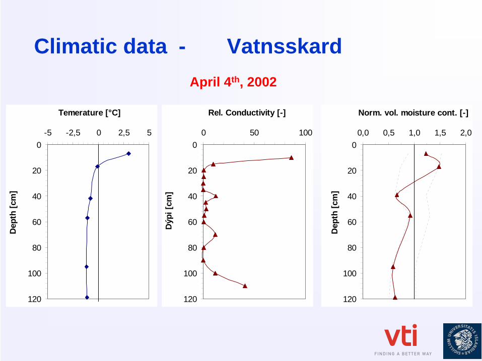
Climatic data - Vatnsskard

0

20

40

60

80

100

120

-5 -2,5 0 2,5 5

Temerature [°C]

Dep

th [c

m]

0

20

40

60

80

100

120

0 50 100

Rel. Conductivity [-]

Dýp

i [cm

]

0

20

40

60

80

100

120

0,0 0,5 1,0 1,5 2,0

Norm. vol. moisture cont. [-]

Dep

th [c

m]

April 4th, 2002

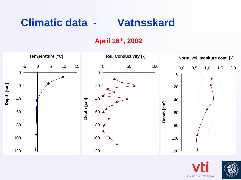
Climatic data - Vatnsskard

0

20

40

60

80

100

120

-5 0 5 10 15

Temperature [°C]

Dep

th [c

m]

0

20

40

60

80

100

120

0 50 100

Rel. Conductivity [-]

Dep

th [c

m]

0

20

40

60

80

100

120

0,0 0,5 1,0 1,5 2,0

Norm. vol. mositure cont. [-]

Dep

th [c

m]

April 16th, 2002

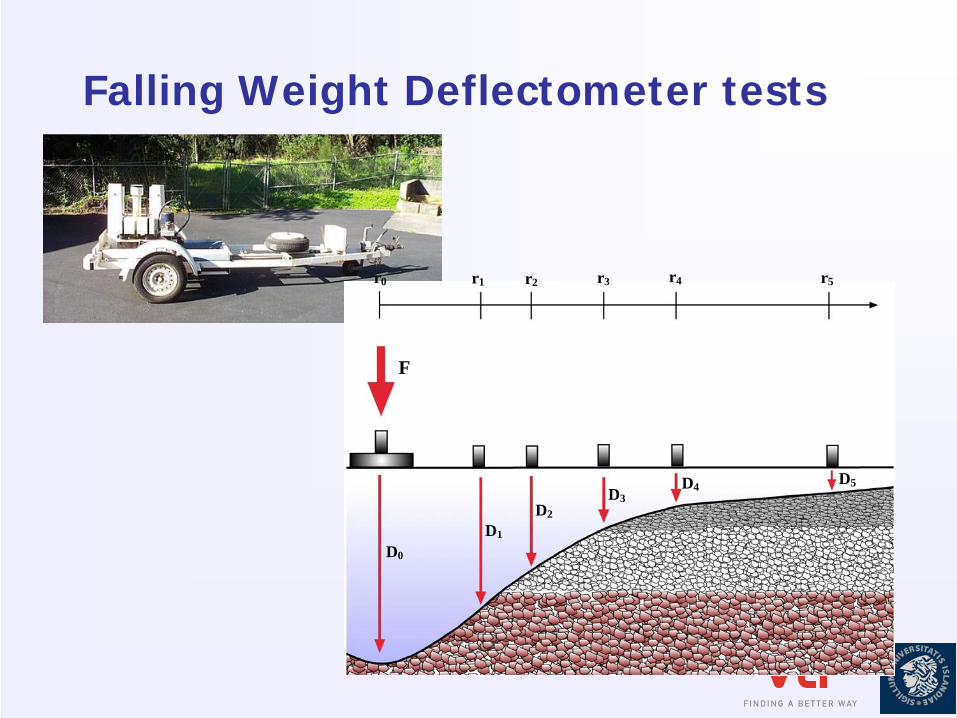
Falling Weight Deflectometer tests

r0 r1 r2 r3 r4 r5

D0

D1

D 2 D3

D4 D5

F

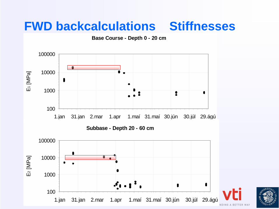
FWD backcalculations StiffnessesBase Course - Depth 0 - 20 cm

100

1000

10000

100000

1.jan 31.jan 2.mar 1.apr 1.maí 31.maí 30.jún 30.júl 29.ágú

E1 [M

Pa]

Subbase - Depth 20 - 60 cm

100

1000

10000

100000

1.jan 31.jan 2.mar 1.apr 1.maí 31.maí 30.jún 30.júl 29.ágú

E2 [M

Pa]

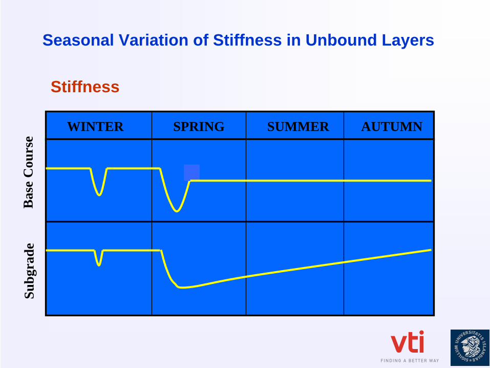
Seasonal Variation of Stiffness in Unbound Layers

WINTER SPRING SUMMER AUTUMN

Subg

rade

Bas

e C

ours

e

Stiffness

Validation

Full scale testing

Accelerated Pavement Testing

• Purpose

To increase the understanding of pavements performance under heavy loading conditions.

Heavy Vehicle Simulator

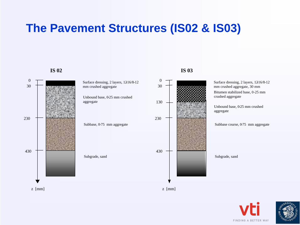
The Pavement Structures (IS02 & IS03)

Surface dressing, 2 layers, 12-16/8-12 mm crushed aggregate

230

430

z [mm]

Subbase, 0-75 mm aggregate

Subgrade, sand

Unbound base, 0-25 mm crushed aggregate

030

Surface dressing, 2 layers, 12-16/8-12 mm crushed aggregate, 30 mm

230

430

z [mm]

Subbase course, 0-75 mm aggregate

Subgrade, sand

Unbound base, 0-25 mm crushed aggregate

030

Bitumen stabilized base, 0-25 mm crushed aggregate

130

IS 02 IS 03

Response Testing - Numerical Simulations

• 2-D Axi & 3-D analysis.

• MLET & FEM analyses

• Linear and non-linear base behaviour

• Distress prediction

IS02 – Single wheel, p = 800 kPa FEM: Vertical displacement

IS02 Vertical Stresses vs. Depth

Depth [cm]

0.0

Surface dressing

Unbound base course

Subbase

Subgrade

1.2

20.3

39.7

Single wheel Dual wheel

Profile 1 Profile 2 Profile 3

W = 120 kN 0

10

20

30

40

50

0 200 400 600 800 1000Stress σz [kPa]

Dep

th [c

m]

Measurements3D FEM LE2D Axi MLET LE2D Axi MLET NLE2D Axi FE LA2D Axi FE NLE

p = 900 kPa

Conclusions

• Mechanistic - empirical based design methods are under development in many countries and will therefore probably be in use in the near future. To be able to use such methods we need to obtain information for modelling purposes on factors affecting pavement performances, such as– Axle loading – Material properties – Weather and environmental conditions

• Further we need information to calibrate and validate such methods if acceptable agreement between real performance and our estimation is to be achieved.

Conclusions cont.

• What will we gain– Far more realistic pavement characterization– Better understanding of pavement performances– Effects of new loading conditions such as increased loads,

higher tyre pressure and multiple axle, can easily be estimated

– Future enhanced or improved knowledge can be easily implemented