accuracy in mechanistic pavement design consequent upon
TRANSCRIPT

University of Nottingham
School of Civil Engineering
Accuracy in Mechanistic Pavement Design
Consequent upon Unbound Material Testing
by Simon D Gillett, BSc (Eng)
University of Nottingham Roughton International, Southampton
Thesis submitted to the University of Nottingham for the degree of Doctor of Philosophy
May 2001


Accuracy in Mechanistic Pavement Design
PhD Thesis Page i
Table of Contents Page No. Abstract
1 An Introduction to the Analysis of Pavements.......................... 1-1
1.1 HISTORY OF ROADS....................................................................................... 1-1 1.2 DESCRIPTION OF THE ROAD STRUCTURE ........................................................ 1-2
1.2.1 The Foundation .............................................................................. 1-3 1.2.2 The Pavement Structural Layers.................................................... 1-3 1.2.3 The Surface .................................................................................... 1-4 1.2.4 Thesis Focus .................................................................................. 1-5
1.3 TECHNICAL BACKGROUND.............................................................................. 1-5 1.3.1 Road Construction Materials .......................................................... 1-5 1.3.2 Pavement Design Methods ............................................................ 1-6 1.3.3 Stress and Strain Determination .................................................... 1-8 1.3.4 Shell Pavement Design Method ..................................................... 1-8 1.3.5 Finite Element Approach ................................................................ 1-9 1.3.6 Pavement Failure Mechanisms .................................................... 1-11
1.4 MATERIALS TESTED DURING THE STUDY ....................................................... 1-12 1.5 THE EUROPEAN ‘SCIENCE PROJECT’ ............................................................ 1-12 1.6 SCOPE OF THIS DISSERTATION ..................................................................... 1-13 1.7 LIMITATION OF THIS WORK ........................................................................... 1-16 1.8 THE ORGANISATION OF THIS DISSERTATION .................................................. 1-16
2 Flexible Pavement Design Procedures ...................................... 2-1
2.1 INTRODUCTION .............................................................................................. 2-1 2.2 EMPIRICAL PAVEMENT DESIGN METHODS ....................................................... 2-2 2.3 MECHANISTIC PAVEMENT DESIGN METHODS................................................... 2-3 2.4 LABORATORY TESTS FOR MATERIAL CHARACTERISATION ................................ 2-7
2.4.1 Standard (Common) Laboratory Materials Tests ........................... 2-7 2.4.2 Non-Standard Laboratory Testing ................................................ 2-10 2.4.3 Verification by Field Testing ......................................................... 2-13
2.5 THE QUANTIFICATION OF MATERIAL PARAMETERS FOR USE IN MECHANISTIC PAVEMENT DESIGN METHODS ...................................................................... 2-14 2.5.1 Characteristic Stresses ................................................................ 2-15 2.5.2 Distribution of Stresses in Pavements.......................................... 2-16
2.6 THE QUANTIFICATION OF FLEXIBLE PAVEMENT STRUCTURES UNDER TRAFFIC LOADING........................................................................................ 2-16 2.6.1 The Behaviour of Bituminous Surfaces and Bases...................... 2-17 2.6.2 The Behaviour of Unbound Granular Bases and Subbases ........ 2-19 2.6.3 The Behaviour of Subgrade Soils and Selected Layers............... 2-22 2.6.4 The Magnitude of Characteristic Stress ....................................... 2-23
2.7 SUMMARY ................................................................................................... 2-28

Accuracy in Mechanistic Pavement Design
Page ii S.D.Gillett
3 Stresses and Strains in Road Pavement Materials ................... 3-1
3.1 INTRODUCTION ...............................................................................................3-1 3.2 STRESSES AND STRAINS IN FLEXIBLE PAVEMENTS ...........................................3-3
3.2.1 General Three Dimensional States of Stress..................................3-3 3.2.2 Vehicular Loading Characteristics ..................................................3-4
3.3 THE BEHAVIOUR OF PAVEMENT MATERIALS UNDER TRAFFIC LOADING ..............3-7 3.3.1 Subgrade Soils ................................................................................3-7 3.3.2 Unbound Granular Materials ...........................................................3-8
3.4 REPEATED LOAD TRIAXIAL TESTING ................................................................3-9 3.4.1 Repeated Load Triaxial Apparatus Configurations .......................3-10 3.4.2 Variable Confining Pressure versus Constant Confining
Pressure ........................................................................................3-13 3.4.3 Apparatus Produced Factors that Influence the Triaxial Test
Results ..........................................................................................3-14 3.4.4 Triaxial Stress State ......................................................................3-18 3.4.5 Resilient Modulus and Poisson’s Ratio.........................................3-25
3.5 SUMMARY ....................................................................................................3-28
4 Factors that Influence the Behaviour of Materials in Pavements .................................................................................... 4-1
4.1 INTRODUCTION ...............................................................................................4-1 4.2 ENVIRONMENTAL CONDITIONS (MOISTURE IN PAVEMENTS)...............................4-1
4.2.1 Principles of Unbound Material and Water Interaction ...................4-2 4.2.2 Suction ............................................................................................4-5 4.2.3 Material Stiffness Related to Water Content...................................4-6
4.3 COMPACTION (DENSITY) OF PAVEMENT LAYERS ..............................................4-9 4.3.1 Compaction of Granular Bases.....................................................4-10 4.3.2 Compaction of Cohesive Subgrade ..............................................4-11
4.4 THE EFFECT OF STRESS LEVELS...................................................................4-11 4.5 LOAD DURATION AND FREQUENCY ................................................................4-12 4.6 LOADING HISTORY........................................................................................4-13 4.7 THE EFFECT OF MATERIAL PROPERTIES ........................................................4-13 4.8 SUMMARY ....................................................................................................4-14
5 Analysis of the Behaviour of the Materials by Modelling ......... 5-1
5.1 INTRODUCTION ...............................................................................................5-1 5.2 MODELLING THE EXPERIMENTAL DATA ............................................................5-1 5.3 CONSTITUTIVE RELATIONSHIPS TO DEFINE THE BEHAVIOUR OF MATERIALS.......5-6
5.3.1 Models for all Road Construction Materials ....................................5-6 5.3.2 For Fine Grained Subgrade Soils used in Road Construction........5-8 5.3.3 For Unbound Granular Materials used in Road Construction.........5-9
5.4 SUMMARY ....................................................................................................5-12
Accuracy in Mechanistic Pavement Design
PhD Thesis Page iii
6 Triaxial Test Apparatus................................................................ 6-1
6.1 INTRODUCTION .............................................................................................. 6-1 6.2 COMMON METHODS OF MEASURING STRAIN ON SPECIMENS IN THE
LABORATORY................................................................................................. 6-1 6.2.1 Spring-Loaded Rings...................................................................... 6-2 6.2.2 Studs and Pins ............................................................................... 6-3 6.2.3 Non-Contacting Sensors ................................................................ 6-3
6.3 APPARATUS AND EQUIPMENT USED DURING THIS WORK ................................. 6-5 6.4 UNIVERSITY OF NOTTINGHAM ......................................................................... 6-5
6.4.1 Variable Confining Pressure Apparatus (150 mm x 76 ∅mm) for Testing of Subgrade Soils ......................................................... 6-5
6.4.2 Variable Confining Pressure Apparatus (300 mm x 150 ∅mm) for Testing Unbound Granular Materials ........................................ 6-8
6.5 LABORATÓRIO NACIONAL DE ENGENHARIA CIVIL ........................................... 6-11 6.5.1 Variable Confining Pressure Apparatus (150 mm x 76 ∅mm)
for Testing of Subgrade Soils ....................................................... 6-12 6.5.2 Constant Confining Pressure Apparatus (600 mm x
300 ∅mm) for Testing Unbound Granular Materials.................... 6-12 6.6 LABORATOIRE REGIONAL DES PONTS ET CHAUSSÉES ................................... 6-15
6.6.2 Variable Confining Pressure Apparatus (150 mm x 70 ∅mm) for Testing of Subgrade Soils ....................................................... 6-16
6.6.3 Variable Confining Pressure Apparatus (320 mm x 160 ∅mm) for Testing Unbound Granular Materials ...................................... 6-19
6.7 DELFT UNIVERSITY OF TECHNOLOGY ............................................................ 6-21 6.7.1 Constant Confining Pressure Apparatus (200 mm x
100 ∅mm) for Testing of Subgrade Soils..................................... 6-21 6.7.2 Constant Confining Pressure Apparatus (800 mm x
400 ∅mm) for Testing Unbound Granular Materials.................... 6-22 6.8 COMPARISON OF THE APPARATUS AND INSTRUMENTATION SYSTEMS ............. 6-25
6.8.1 Instrumentation Fixing Methods ................................................... 6-27 6.9 PHASE 4 - INSTRUMENTATION COMPARISON ON THE ARTIFICIAL SPECIMEN..... 6-31 6.10 INSTRUMENTATION LIMITATIONS ................................................................... 6-35 6.11 ASSESSING INACCURACIES IN LABORATORY TESTING OF MATERIALS.............. 6-36
6.11.1 Identifying Errors .......................................................................... 6-36 6.11.2 Errors Occurring During the Manufacture of the Specimen ......... 6-37 6.11.3 Errors Occurring During the Repeated Load Triaxial Testing ...... 6-38 6.11.4 Errors Occurring During the Analysis of the Results.................... 6-39
6.12 BASIC STATISTICS........................................................................................ 6-39 6.13 SUMMARY ................................................................................................... 6-42

Accuracy in Mechanistic Pavement Design
Page iv S.D.Gillett
7 The Triaxial Test Procedures and Results ................................. 7-1
7.1 INTRODUCTION ...............................................................................................7-1 7.2 OTHER TEST PROCEDURES FOR THE CHARACTERISATION ................................7-1
7.2.1 Test Procedures for Granular Materials..........................................7-1 7.2.2 Test Procedures for Subgrade Materials ........................................7-4
7.3 PHASE 1 - FIRST INTER-LABORATORY COMPARISON.........................................7-5 7.4 PHASE 2 - SECOND INTER-LABORATORY COMPARISON ..................................7-14
7.4.1 Permanent Strain Behaviour .........................................................7-17 7.4.2 Resilient Strain Behaviour.............................................................7-20
7.5 PHASE 3 - ROUND ROBIN TESTING ON THE ARTIFICIAL SPECIMEN ...................7-27 7.6 PHASE 5 - THE PRINCIPAL TEST PROGRAMME ...............................................7-34 7.7 COMPARISON OF METHODS SPECIMEN MANUFACTURE ..................................7-35
7.7.1 Subgrade Soils ..............................................................................7-35 7.7.2 Unbound Granular Materials .........................................................7-38
7.8 SUMMARY ....................................................................................................7-39
8 Analysis of the Behaviour of the Materials by Analytical Modelling ...................................................................................... 8-1
8.1 INTRODUCTION ...............................................................................................8-1 8.2 DATA VERIFICATION AND MANIPULATION..........................................................8-1
8.2.1 Initial Screening (Removal of Obviously Poor Data).......................8-2 8.2.2 Secondary Screening (Removal of Outliers by Percentile).............8-3 8.2.3 Analytical Modelling Methods Used to Model the Results ..............8-5
8.3 PRESENTATION OF THE RESULTS ....................................................................8-6 8.3.1 Modelling Analyses to determine the Material Coefficients ............8-6 8.3.2 Analysis of the Test Results and Comparison Method .................8-10 8.3.3 Actual Removal of the Outliers from the Test Results ..................8-13 8.3.4 Comparison of the Results as the Data is Reduced by
Removal of Outliers.......................................................................8-19 8.3.5 Comparison of Identical Data Analysed using Different
Analytical Methods ........................................................................8-25 8.3.6 Comparison of the Same Material Tested at Different
Laboratories ..................................................................................8-28 8.3.7 Comparison of Different Specimens of the Same Material
Tested within a Single Laboratory.................................................8-32 8.4 INTRODUCTION OF RANDOM ERRORS TO DATA...............................................8-38 8.5 FINAL VALUES FROM THE TESTING AND ANALYSIS ..........................................8-42 8.6 SUMMARY ....................................................................................................8-45
Accuracy in Mechanistic Pavement Design
PhD Thesis Page v
9 Design of Flexible Pavements Using the Test Results ............. 9-1
9.1 INTRODUCTION .............................................................................................. 9-1 9.2 THE STRUCTURAL ANALYSIS OF SPECIFIC PAVEMENTS.................................... 9-4 9.3 THE INFLUENCE OF THE MATERIAL VARIATIONS TO PAVEMENT DESIGN........... 9-12
9.3.1 Comparison 1 - Variation of the Base Strength from Four Different Laboratories ................................................................... 9-17
9.3.2 Comparison 2 - Variation of the Subgrade Strength from Four Different Laboratories ................................................................... 9-20
9.3.3 Comparison 3 and 4- Variation of the range of Values of the Base and Subgrade Material Characteristics Conducted at a Single Laboratory ......................................................................... 9-26
9.3.4 Comparison 5 - Variation with the Introduction of a Random Error into the Strain Measurements ............................................. 9-30
9.4 SUMMARY ................................................................................................... 9-30
10 Summary and Conclusions ....................................................... 10-1
10.1 SUMMARY ................................................................................................... 10-1 10.2 DISCUSSION ................................................................................................ 10-3 10.3 CONCLUSIONS ........................................................................................... 10-12 10.4 RECOMMENDATIONS FOR FUTURE WORK.................................................... 10-15
11 References.................................................................................. 11-1
12 Appendices................................................................................. 12-1

Accuracy in Mechanistic Pavement Design
Page vi S.D.Gillett
List of Tables Page No. Table 1-1 Materials Tested under the Various Test Programmes........................1-12 Table 2-1 Summary of the Analytical Structural Pavement Criteria........................2-7 Table 2-2 Approximate Stiffness Values for Asphalt at Representative
Vehicle Speeds and Surface Temperatures.........................................2-18 Table 2-3 Approximate Stiffness Values for Varying Asphalt Mixes.....................2-19 Table 2-4 Approximate Resilient Moduli for Granular Materials at Various
Moisture Conditions ..............................................................................2-20 Table 2-5 Approximate Resilient Moduli of Subgrade Materials at Different
Moisture Conditions ..............................................................................2-22 Table 2-6 Determination of the Characteristic Stresses for a Characteristic
Pavement ..............................................................................................2-27 Table 6-1 Summary of Triaxial Apparatus of the Participating Laboratories ........6-28 Table 6-2 Static Stress Regime applied during Instrumentation Comparison......6-31 Table 6-3 Dynamic Stress Regime applied during Instrumentation
Comparison...........................................................................................6-32 Table 6-4 Instrumentation Tested during the Single-Specimen Comparison.......6-32 Table 6-5 Instrumentation Comparative Results on Artificial Specimen...............6-34 Table 6-6 Summary of the Advantages and Disadvantages of Various
Instrumentation Methods ......................................................................6-43 Table 6-7 Summary of the Advantages and Disadvantages of Various
Apparatus Methods...............................................................................6-44 Table 7-1 Test Procedure I for the Subgrade Soils.................................................7-6 Table 7-2 Test Procedure I for the Unbound Granular Materials ...........................7-7 Table 7-3 Stress Paths Test Programme I for a Hard Limestone (CCT)..............7-10 Table 7-4 The Range of Normalised Axial and Radial Strain measured at
Different Laboratories for Hard Limestone ...........................................7-13 Table 7-5 Materials Characteristics as Tested in Phase 2 ...................................7-14 Table 7-6 Test Procedure II for the Subgrade Soils..............................................7-15 Table 7-7 Test Procedure II for the Unbound Granular Materials ........................7-16 Table 7-8 Compaction Methods Specified ............................................................7-17 Table 7-9 Comparison of the Permanent Axial Strain for Unbound Granular
Specimens ............................................................................................7-18 Table 7-10 Comparison of the Resilient Axial Strain for Unbound Granular
Specimens (TP2) ..................................................................................7-20 Table 7-11 Comparison of the Resilient Radial Strain for Unbound Granular
Specimens (TP2) ..................................................................................7-23 Table 7-12 Comparison of the Permanent Strains for Subgrade Soil
Specimens (TP2) ..................................................................................7-24 Table 7-13 Comparison of the Axial Strains for London Clay Specimens (TP2)....7-25 Table 7-14 Comparison of the Resilient Strains London Clay Specimens (TP2) ...7-25 Table 7-15 Comparison of the Resilient Modulus for Subgrade Soil Specimens
(TP2) .....................................................................................................7-26 Table 7-16 Loading Regime Applied to the Artificial Specimen..............................7-27 Table 7-17 The Apparatus and the Corresponding Specimen Size .......................7-28

Accuracy in Mechanistic Pavement Design
PhD Thesis Page vii
Table 7-18 Recorded Stresses Applied to the Artificial Specimen......................... 7-28 Table 7-19 The Average and Minimum Instrumentation Wandering ..................... 7-30 Table 7-20 Recorded Strains on the Artificial Specimen........................................ 7-33 Table 7-21 Resilient Moduli and Poison's Ratio for the Artificial Specimen........... 7-34 Table 7-22 Test Procedure III for the Subgrade Soils............................................ 7-36 Table 7-23 Test Procedure III for the Unbound Granular Materials....................... 7-37 Table 8-1 Removal of Poor Data and Outliers from the Test Data ........................ 8-5 Table 8-2 Example of the Presentation of the Model Analysis for Subgrade
Soils........................................................................................................ 8-8 Table 8-3 Example of the Presentation of the Model Analysis for Unbound
Granular Materials.................................................................................. 8-9 Table 8-4 Limiting Criteria for the Parameters and Model Coefficients ............... 8-13 Table 8-5 The Results of Fontainebleau Sand tested in Test Programme I
and Analysed as a Subgrade Soil ........................................................ 8-14 Table 8-6 The Results of Fontainebleau Sand tested in Test Programme I
and Analysed as a Granular Material................................................... 8-16 Table 8-7 Correlation Coefficients at Various Outlier Removal Percentile
Values for a Specimen of Fontainebleau Sand and Hard Limestone.. 8-22 Table 8-8 Summary of the Trends of the Correlation Coefficients for the
Removal of Outliers for Test Programme I .......................................... 8-23 Table 8-9 Characteristic Resilient Modulus for Fontainebleau Sand Analysed
by two Different Methods ..................................................................... 8-25 Table 8-10 Variation of Resilient Moduli when Predicted by Different Methods
of Modelling .......................................................................................... 8-28 Table 8-11 Results of Test Programme II on Subgrade Soil – London Clay ......... 8-30 Table 8-12 Results of Test Programme II on Unbound Granular Material -
Microgranite.......................................................................................... 8-31 Table 8-13 Summary of the Test Programme II Subgrade Soil Results ................ 8-32 Table 8-14 Summary of the Test Programme II Unbound Granular Material –
Microgranite Results ............................................................................ 8-32 Table 8-15 Variation from the Average for Average Modelled and Specimen
Characteristic Values ........................................................................... 8-33 Table 8-16 Results of Test Programme III on Subgrade Soil – London Clay ........ 8-34 Table 8-17 Results of Test Programme III on Subgrade Soil – Seine et Marne
Silt......................................................................................................... 8-35 Table 8-18 Results of Test Programme III on Unbound Granular Material –
Soft Limestone Results ........................................................................ 8-36 Table 8-19 Results of Test Programme III on Unbound Granular Material –
Hard Limestone Results....................................................................... 8-37 Table 8-20 Final Parameters and Coefficients for the Subgrade Soils .................. 8-43 Table 8-21 Final Parameters and Coefficients for the Unbound Granular
Materials............................................................................................... 8-44 Table 9-1 Ranking of the Materials Tested in Terms of Quality ............................. 9-5 Table 9-2 Pavement Structure and Characterisation Model for each Layer.......... 9-7 Table 9-3 Pavement Structures with Different Material Characteristics that
were Analysed...................................................................................... 9-13 Table 9-4 Analyses Conducted showing when Successful Solutions were
Achieved............................................................................................... 9-14

Accuracy in Mechanistic Pavement Design
Page viii S.D.Gillett
Table 9-5 Summary of the Mechanistic Analysis Run Results .............................9-15 Table 9-6 Mechanistic Analysis with Varying Material Characteristics showing
Successful Solutions.............................................................................9-16 Table 9-7 Mechanistic Analysis with Random Errors Introduced showing
Successful Solutions.............................................................................9-16

Accuracy in Mechanistic Pavement Design
PhD Thesis Page ix
List of Figures Page No. Figure 1-1 A Typical Pavement Structure for a Flexible Pavement......................... 1-3 Figure 2-1 Pavement Failure Criteria for Mechanistic Design................................. 2-4 Figure 2-2 A Simplified Mechanistic Design Approach ........................................... 2-6 Figure 2-3 Schematic Representation of a Triaxial Specimen under an
Applied Load ........................................................................................ 2-11 Figure 2-4 Stress Levels Applied at Different Points in a Pavement..................... 2-15 Figure 2-5 Trend for the Relationship between Horizontal Tensile Strain
(Fatigue) Criteria and Traffic Loading for Asphalt Surfacing and Base ..................................................................................................... 2-18
Figure 2-6 Trend for the Relationship between Factor of Safety (Shear Strength) Criterion and Traffic Loading for Unbound Granular Materials............................................................................................... 2-21
Figure 2-7 Trend for the Relationship between Compressive Strain Criteria for Subgrade Deformation and Traffic Loading ......................................... 2-23
Figure 2-8 Materials and Pavement Details for the Calculation of Characteristic Stresses ........................................................................ 2-24
Figure 2-9 The Sensitivity of the Resilient Moduli and Poisson’s Ration values to Re-Analysis ...................................................................................... 2-25
Figure 2-10 The Self Weight Characteristic Stress within a Typical European Pavement Structure.............................................................................. 2-26
Figure 2-11 The Characteristic Stress within a Typical European Pavement Structure............................................................................................... 2-27
Figure 3-1 Loading in Pavements under Traffic ...................................................... 3-2 Figure 3-2 The Stress-Strain Behaviour of Materials under Repeated Loading. .... 3-3 Figure 3-3 Loading of an Element in a Pavement Showing the Rotation of the
Principal Stresses................................................................................... 3-4 Figure 3-4 Pavement Loading Characteristics ........................................................ 3-5 Figure 3-5 Vertical Stress Pulse Time as a Function of the Depth in a
Pavement for different Vehicle Speeds.................................................. 3-6 Figure 3-6 Schematic Illustration of the Repeated Load Triaxial Apparatus ......... 3-11 Figure 3-7 The Definition of a Stress Path in p-q Space ....................................... 3-23 Figure 3-8 Possible Stress Regimes in a Repeated Loads Triaxial Test .............. 3-24 Figure 3-9 Uniaxial Stress Condition Hooke’s Law ............................................... 3-26 Figure 4-1 Pore Pressure in Pavements ................................................................. 4-3 Figure 5-1 Definition of Linearity and Elasticity ....................................................... 5-3 Figure 5-2 Stress Dependency of the Resilient Modulus and Poisson’s Ratio
for a Sample of London Clay.................................................................. 5-4 Figure 5-3 Stress Dependency of the Resilient Modulus and Poisson’s Ratio
for a Sample of Soft Limestone.............................................................. 5-5 Figure 5-4 Determination of the p* Coefficient ...................................................... 5-10 Figure 6-1 University of Nottingham - Variable Confining Pressure Apparatus
(150 mm x 76 ∅mm) .............................................................................. 6-9

Accuracy in Mechanistic Pavement Design
Page x S.D.Gillett
Figure 6-2 University of Nottingham - Variable Confining Pressure (300 mm x 150∅ mm) .............................................................................................6-10
Figure 6-3 Laboratório Nacional de Engenharia Civil - Constant Confining Pressure Apparatus (600 mm x 300 ∅mm)..........................................6-13
Figure 6-4 Laboratoire Regional Des Ponts et Chaussées - Variable Confining Pressure Apparatus (150 mm x 70 ∅mm)............................................6-18
Figure 6-5 Laboratoire Regional Des Ponts et Chaussées -Variable Confining Pressure Apparatus (320 mm x 160 ∅mm)..........................................6-20
Figure 6-6 Delft University of Technology - Constant Confining Pressure Apparatus (200 mm x 100 ∅mm) .........................................................6-22
Figure 6-7 Delft University of Technology - Constant Confining Pressure Apparatus (800 mm x 400 ∅mm) .........................................................6-24
Figure 6-8 Instrumentation Layout for the Repeated Load Triaxial Apparatus ......6-26 Figure 6-9 Instrumentation Comparison showing differing Strain and Stress
Conditions .............................................................................................6-33 Figure 7-1 Graphic Representation of Intended Stress Paths for Test
Procedure I (Subgrade Soils) .................................................................7-8 Figure 7-2 Graphic Representation of Intended Stress Paths for Test
Procedure I (Unbound Granular Materials) ............................................7-8 Figure 7-3 Comparison of the Deviator Stresses Applied compared to that
Specified for Different Laboratories for Hard Limestone ......................7-10 Figure 7-4 Comparison of the Axial Strain Measured at Different Laboratories
for a Specimen of Hard Limestone .......................................................7-11 Figure 7-5 Comparison of the Radial Strain Measured at Different
Laboratories for a Specimen of Hard Limestone ..................................7-12 Figure 7-6 Comparative Strain Reading Normalised with Deviator Stress
Paths for a Specimen of Hard Limestone.............................................7-12 Figure 7-7 Permanent Strains Measured in Different Apparatus while testing
Microgranite ..........................................................................................7-19 Figure 7-8 Resilient Strains Measured on Specimens of Subgrade Soil during
Test Programme II ................................................................................7-21 Figure 7-9 Resilient Strains Measured on Specimens of Unbound Granular
Base during Test Programme II............................................................7-22 Figure 7-10 Artificial Specimen Test 1 .....................................................................7-29 Figure 7-11 Artificial Specimen Test 2 .....................................................................7-31 Figure 7-12 Artificial Specimen Test 3 .....................................................................7-32 Figure 8-1 Comparison of the Experimental and Modelled Resilient Modulus
for an Unbound Granular Material ..........................................................8-3 Figure 8-2 Comparison of the Experimental and Modelled Resilient Modulus
for a Subgrade Soil .................................................................................8-3 Figure 8-3 Material Coefficient as a Percentile of Resilient Modulus for
Fontainebleau Sand tested in Test Programme I .................................8-19 Figure 8-4 Comparison for all Stress Paths showing Probable outliers for a
Specimen of Fontainebleau Sand.........................................................8-20 Figure 8-5 Comparison for all Stress Paths showing Probable outliers for a
Specimen of Hard Limestone ...............................................................8-20 Figure 8-6 Results from a Specimen of Fontainebleau Sand once the 90%
Outliers have been Removed ...............................................................8-21

Accuracy in Mechanistic Pavement Design
PhD Thesis Page xi
Figure 8-7 Results from a Specimen of Hard Limestone once the 90% Outliers have been Removed............................................................... 8-21
Figure 8-8 Correlation factors for Differing Percentile Values for Fontainebleau Sand Modelled using the k-theta Model....................... 8-24
Figure 8-9 Comparison of Fontainebleau Sand Results Analysed for Different Specimens (Laboratories) .................................................................... 8-27
Figure 8-10 Comparison of Fontainebleau Sand Results Analysed by Different Analytical Methods ............................................................................... 8-27
Figure 8-11 Comparison of the Analysis of London Clay (Test Programme II) tested at four Laboratories ................................................................... 8-29
Figure 8-12 Comparison of the Analysis of Microgranite (Test Programme II) tested at four Laboratories ................................................................... 8-29
Figure 8-13 Analysis of the London Clay Specimens tested at LNEC under Test Programme III............................................................................... 8-34
Figure 8-14 Analysis of the Seine et Marne Specimens Tested at LNEC under Test Programme III............................................................................... 8-35
Figure 8-15 Analysis of the Soft Limestone Specimens Tested at LRSB under Test Programme III............................................................................... 8-36
Figure 8-16 Analysis of the Hard Limestone Specimens Tested at LRSB under Test Programme III............................................................................... 8-37
Figure 8-17 Increase in Scatter as the Variation Increases for a Subgrade Soil .... 8-39 Figure 8-18 Increase in Scatter as the Variation Increases for an Unbound
Granular Material.................................................................................. 8-40 Figure 8-19 Resilient Modulus with changing Error Variation for an Unbound
Granular Material.................................................................................. 8-41 Figure 8-20 Resilient Modulus with changing Error Variation for a Subgrade
Soil........................................................................................................ 8-42 Figure 9-1 Analytical Points for ELSYM5 ................................................................ 9-2 Figure 9-2 Analytical Grid for FENLAP.................................................................... 9-3 Figure 9-3 Mechanistic Analysis of the Pavement Structures Under
Construction (50 mm Asphalt Surface) .................................................. 9-9 Figure 9-4 Mechanistic Analysis of the Pavement Structures In Service
(100 mm Asphalt Surface) ................................................................... 9-10 Figure 9-5 Mechanistic Analysis of the Pavement Structures In Service
(150 mm Asphalt Surface) ................................................................... 9-11 Figure 9-6 Comparison 1 - Variation of the Base Strength from Four Different
Laboratories in Test Programme III...................................................... 9-18 Figure 9-7 Comparison 2 - Variation of the Subgrade Strength from Four
Different Laboratories........................................................................... 9-21 Figure 9-8 Surface Deflection Bowls for a Pavement Structure with a 100 mm
Asphalt Surface .................................................................................... 9-23 Figure 9-9 Surface Deflection Bowls for a Pavement Structure with a 150 mm
Asphalt Surface .................................................................................... 9-24 Figure 9-10 Comparison 3 - Variation within the Range of Values for the Base
Strength at a Single Laboratory ........................................................... 9-28 Figure 9-11 Comparison 4 - Variation within the Range of Values for the
Subgrade Strength at a Single Laboratory........................................... 9-29 Figure 9-12 Comparison 5 - Variation with the Introduction of a Random Error
into the Strain Measurements .............................................................. 9-31

Accuracy in Mechanistic Pavement Design
Page xii S.D.Gillett
List of Photographs Page No. Photograph 3-1 Repeated Load Triaxial Apparatus ..............................................3-11 Photograph 6-1 Apparatus at Nottingham ...............................................................6-6 Photograph 6-2 Apparatus at Lisbon .....................................................................6-11 Photograph 6-3 Apparatus at Saint Brieuc ............................................................6-16 Photograph 6-4 Apparatus at Delft ........................................................................6-21 Photograph 7-1 Specimen Density Measurement at LNEC ..................................7-38

Accuracy in Mechanistic Pavement Design
PhD Thesis Page xiii
Appendices The appendices are contained on a Compact Disk in Adobe Acrobat (pdf) format
bound into the back of this volume together with a copy of Acrobat Reader Version 4.
A copy of this thesis is also contained on the Compact Disk in Adobe Acrobat (pdf)
format.
Appendix A Description and Classification of Materials used in this Study
Appendix B A European Approach to Road Pavement Design
Appendix C Results of the Instrumentation Comparison Experiment Conducted at LRSB (Phase 4)
Appendix D The Test Procedures for Phases 1, 2 and 5
Appendix D.1 The First Test Procedure for testing Subgrade Soils and Unbound Granular Materials (Test Programme I; Phase 1)
Appendix D.2 The Second Test Procedures for testing Subgrade Soils and Unbound Granular Materials (Test Programme II; Phase 2)
Appendix D.3 The Third Test Procedures for testing Subgrade Soils and Unbound Granular Materials (Test Programme III; Phase 5)
Appendix E Results of the Apparatus Comparison using an Artificial Specimen ‘Round Robin’ Experiment (Phase 3)
Appendix F The Repeated Load Triaxial Test Results for Phases 1, 2 and 5
Appendix F.1 Results of Test Programme I for Subgrade Soils and Unbound Granular Materials (Phase 1)
Appendix F.2 Results of Test Programme II for Subgrade Soils and Unbound Granular Materials (Phase 2)
Appendix F.3 Results of Test Programme III for Subgrade Soils and Unbound Granular Materials (Phase 5)

Accuracy in Mechanistic Pavement Design
Page xiv S.D.Gillett
Appendix G The Analysis and Analytical Modelling of the Test Results
Appendix G.1 Results of Test Programme I for Subgrade Soils and Unbound Granular Materials (Phase 1)
Appendix G.2 Results of Test Programme II for Subgrade Soils and Unbound Granular Materials (Phase 2)
Appendix G.3 Results of Test Programme III for Subgrade Soils and Unbound Granular Materials (Phase 5)
Appendix G.4– Summary of the Correlation Coefficients for Test Programme I
Appendix G.5– Introduction of a Random Error of differing Variation to Data
Appendix G.6 Summary of the Analysis Parameters and Coefficients for all of the Test Programmes
Appendix H Mechanistic Pavement Design
Appendix H.1 Mechanistic Pavement Design Analyses
Appendix H.2 Pavement - Life Estimations
Accuracy in Mechanistic Pavement Design
PhD Thesis Page xv
Abstract
As part of a European Union funded research study (the "SCIENCE" project)
performed between 1990 and 1993, granular road construction material and subgrade
soil specimens were tested in the four participating laboratories of the project:
Laboratório Nacional de Engenharia Civil Portugal
University of Nottingham United Kingdom
Laboratoire Central des Ponts et Chaussées France
Delft University of Technology The Netherlands
The author was based the first of these and visited the other participating laboratories,
performing the majority of the work described.
Inaccuracies in repeated load triaxial testing based on the use of different apparatus
and instrumentation are identified. A detailed instrumentation comparison is
undertaken, which results in the magnitude of potential errors being quantified.
The author has derived material parameters and model coefficients for the materials
tested using a number of previously published material models. In order to establish
these parameters a method for removing outliers from test data based on the
difference between the modelled and experimental material parameters for each
stress path applied was developed.
The consequences of repeatability and reproducibility, variability and inaccuracies in
the output of repeated load triaxial testing, on the parameters and, hence, on
computed pavement design thicknesses or life is investigated using a number of
material models and the South African mechanistic pavement design method.

Accuracy in Mechanistic Pavement Design
Page xvi S.D.Gillett
Overall, it is concluded that:
• Instrumentation differences are not as critical as variations in results obtained
from different specimens tested in a single repeated load triaxial apparatus. It was
found that specimen manufacture difference yielded greater variation that
instrumentation differences.
• Variation in results has some effect on the upper granular layers, where higher
stress levels are experienced, but even quite considerable variation in the results
from materials used in the lower layers has little effect on pavement life.
• Analytical methods to determine the stresses and strains vary considerably as do
the predicted pavement thicknesses consequent on using these methods.
The inaccuracies in testing (large discrepancies are found when the same material is
tested in the same laboratory) and the limitations of the available material models
severely limit the usefulness of advanced testing and non-linear modelling in routine
pavement design. On the basis of this study it is recommended that a more simplistic
pavement design approach be taken keeping in line with future developments of
testing and modelling and field validation.

Accuracy in Mechanistic Pavement Design
PhD Thesis Page xvii
Acknowledgements
Acknowledgement is due to the European Community who funded the project ‘A
European Approach to Road Pavement Design’ from which much of this work is
drawn. The author wishes to express his particular thanks to Mr.Andrew Dawson for
his continual guidance and support.
The author is grateful to the staff of the four laboratories for providing all the
necessary facilities, namely:
Laboratório Nacional de Engenharia Civil Portugal
University of Nottingham United Kingdom
Laboratoire Central des Ponts et Chaussées France
Delft University of Technology The Netherlands
The author would like to express his gratitude to all persons and organisations that
contributed to this work with their support, encouragement and advice. In particular,
Dr.Harold Bofinger and Mrs.Pamela Főrs.
A special thank you is due to Roughton International who has continually supported
the author during the compilation of this work.
Finally, special thanks are due to the author's supportive and infinitely patient wife,
Marianne.


Accuracy in Mechanistic Pavement Design Introduction
PhD Thesis Page 1-1
ACCURACY IN MECHANISTIC PAVEMENT DESIGN CONSEQUENT UPON UNBOUND MATERIAL TESTING
1 AN INTRODUCTION TO THE ANALYSIS OF PAVEMENTS
1.1 HISTORY OF ROADS
Roads have been constructed almost since the invention of the wheel; 1800 years ago
the Romans constructed a vast network over much of Europe {Croney and Croney
(1991)}. As wheeled transport replaced pack animals more roads were constructed.
Various construction methods were used from stone set, brick pavements, and
wooden block pavements to the asphalt and concrete that the road pavement
structures comprise today.
The engineers responsible for setting out these early roads would have known
something of the elements of soil mechanics. They would have understood that it was
necessary to remove poor strength material and replace it with superior material; this
imported material required a loading capacity suitable for the proposed loads.
Today’s pavement engineering follows exactly this principle {Transport Research
Laboratory (1993)} using the following three steps:
i) Estimate the amount of traffic loading that will use the road over the selected
design life in years;
ii) Assess the load carrying capacity of the subgrade soil over which the road is to
be built;
iii) Select the most economical combination of road pavement materials and layer
thickness that will provide satisfactory service over the design life of the
pavement without exceeding the subgrade load carrying capacity. It is usually
necessary to assume that an appropriate level of maintenance is also carried
out.
The road infrastructure has over the years, particularly in the last century, become one
of Europe’s most important economic assets. It provides door-to-door transportation
for both people and goods. Recent rapid growth in road traffic numbers and gross

Introduction Accuracy in Mechanistic Pavement Design
Page 1-2 S.D.Gillett
weights of commercial vehicles may lead to premature failures of trunk roads and
motorways, which were not designed for these loads {Loach (1987)}. Vast amounts of
money are invested in the construction and maintenance of a country’s road network
emphasising the importance of good pavement design and management procedures.
Repairs to roads are expensive not only because of the cost of repair but also
because of the extensive delays to private and commercial road users. Poorly
designed road pavements may cause premature failure, however over-designed
pavements waste both limited funds and precious materials. There is a need to
design roads for greater and greater traffic volumes while conserving the limited
natural material resources and therefore a need for a better understanding of the
behaviour of various materials that make up a road pavement structure.
1.2 DESCRIPTION OF THE ROAD STRUCTURE
Road pavement structures are built for the purpose of operating wheeled vehicles
safely and economically, thus forming a reliable road transport system. Pavements
comprise one or more layers of imported material placed over the existing soil. There
are essentially three types of road pavement:
• Unsurfaced pavements with natural gravel wearing coarse surface;
• Flexible pavements these may have thick or thin bituminous surfaces, and;
• Rigid pavements these have concrete bases and surfaces.
This study will only consider flexible pavements since it is these that provide more
than 90% of the road stock in most European countries. The structural format of a
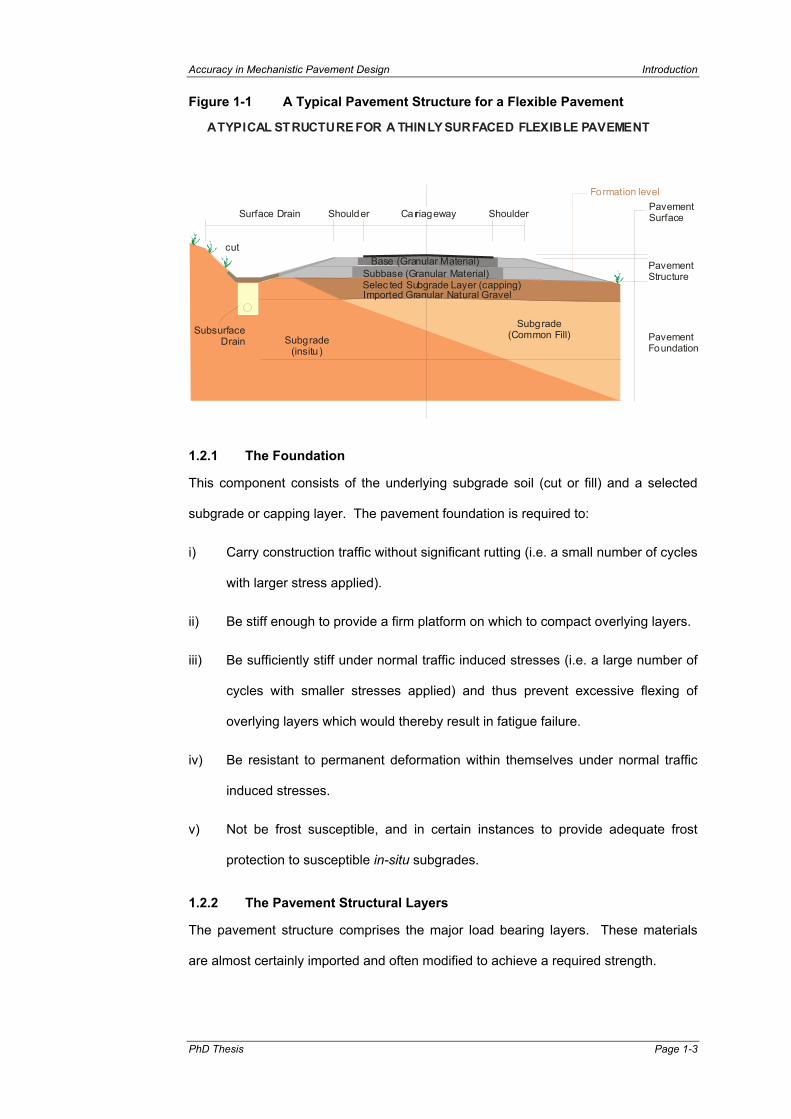
flexible pavement is shown in a schematic road cross-section in Figure 1-1.
These layers can be combined and simplified with the assumption that all road
pavements have essentially three components, namely:
• The foundation;
• The pavement structural layers, and;
• The surfacing.
Accuracy in Mechanistic Pavement Design Introduction
PhD Thesis Page 1-3
Figure 1-1 A Typical Pavement Structure for a Flexible Pavement
A TYPICAL STRUCTURE FOR A THINLY SURFACED FLEXIBLE PAVEMENT
Surface Drain
SubsurfaceDrain
Shoulder ShoulderCarriagewayPavementSurface
Formation level
Subgrade(Common Fill)Subgrade
(insitu)
Selec ted Subgrade Layer (capping)Subbase (Granular Material)
Base (Granular Material)cut
Imported Granular Natural Gravel
PavementStructure
PavementFoundation
1.2.1 The Foundation
This component consists of the underlying subgrade soil (cut or fill) and a selected
subgrade or capping layer. The pavement foundation is required to:
i) Carry construction traffic without significant rutting (i.e. a small number of cycles
with larger stress applied).
ii) Be stiff enough to provide a firm platform on which to compact overlying layers.
iii) Be sufficiently stiff under normal traffic induced stresses (i.e. a large number of
cycles with smaller stresses applied) and thus prevent excessive flexing of
overlying layers which would thereby result in fatigue failure.
iv) Be resistant to permanent deformation within themselves under normal traffic
induced stresses.
v) Not be frost susceptible, and in certain instances to provide adequate frost
protection to susceptible in-situ subgrades.
1.2.2 The Pavement Structural Layers
The pavement structure comprises the major load bearing layers. These materials
are almost certainly imported and often modified to achieve a required strength.

Introduction Accuracy in Mechanistic Pavement Design
Page 1-4 S.D.Gillett
The subbase is the secondary load-spreading layer underlying the base. It will
normally consist of a material of lower quality than that used in the base. This layer
also serves as a separating layer preventing contamination of the base by the
subgrade material and, under wet conditions, it has an important role to play in
protecting the subgrade from damage by construction traffic.
The base is the main structural element of the road pavement. It is required to spread
the wheel load so that underlying material is not over-stressed. The base in flexible
construction may be of dense bituminous material or lean concrete but, in many cases
for more lightly trafficked roads, cheaper Unbound Granular Material (UGM) may be
adequate.
In summary these layers must, under normal traffic loading, be:
i) Sufficiently stiff to spread the load well and thus prevent over-stressing of
underlying layers.
ii) Stiff enough to prevent fatigue failure of any overlying layers.
iii) Able to resist permanent deformation within their thickness.
iv) If bound, have adequate fatigue life.
A substantial amount of research has been done on bound base layers, both
bituminous and lean concrete such that the structural behaviour of bound materials is
relatively well understood and documented. Acceptable material models can be used
readily in the various design methods available for example the Nottingham Pavement
Design Method {Brown and Brunton (1990)}.
1.2.3 The Surface
The surfacing is principally to provide adequate protection to the base, to reduce
water ingress into the pavement and to provide skid resistance and riding quality to
vehicles that travel along the road. The surface generally has little structural
significance and will not be considered in detail in this work. However, in the case
where it will make some contribution to the structural integrity of the pavement, it will
be taken to be a component part of the base layer. For example, when a 40 to 60 mm
Accuracy in Mechanistic Pavement Design Introduction
PhD Thesis Page 1-5
layer of dense bituminous mixture surface is used the base thickness will be
effectively increased by an amount related to the thickness of the surface. The
characteristics of the base will then be used for the total layer thickness.
1.2.4 Thesis Focus
This thesis concentrates on the unbound granular materials that are used for
structural base and subbase layers in pavements and the unbound subgrade soils
that occur in road foundations pavements (selected subgrade and subgrade). Details
of the thesis scope and aims are given later in Chapter 1.6.
1.3 TECHNICAL BACKGROUND
In recent years a number of important empirical studies {Parsley and Robinson
(1982); Paterson (1987); Chesher and Harrison (1987), Watanatada et al (1987)}
have shown how the costs of operating vehicles depend on the surface condition of
the road. The studies have also improved the knowledge of how the deterioration of
roads depends on the nature of the traffic, the properties of the road construction
materials, the environment, and the maintenance strategy adopted.
In present times, when economic considerations control road construction, every
proposed road construction and rehabilitation project is economically analysed with
rigour against many similar projects and only relatively few construction projects are
funded. Ideally only the best quality materials would be used for the construction of
road pavements, however these materials are expensive and the need to construct
more economic roads is becoming more significant as material shortages occur. In
the light of this it is very important to use the most economical materials possible for
the construction, yielding a road that is neither over-designed nor will fail before the
design period (the proposed period of usage) is complete.
1.3.1 Road Construction Materials
A wide variety of materials is used for the construction of road pavements. These
vary from crushed quarried rock through to crushed and screened natural gravel.
Good quality naturally occurring ‘as dug’ gravel can be mechanically stabilised and
modified. Poorer quality naturally occurring materials are often either mechanically

Introduction Accuracy in Mechanistic Pavement Design
Page 1-6 S.D.Gillett
stabilised or stabilised using a chemical stabilising agent such as lime or cement (this
involves the addition of a stabilising agent, mixing with sufficient water, compaction
and final curing to ensure that the mechanical potential is realised).
In many areas good quality materials are rare and haul costs can be high, therefore
more marginal quality materials may need to be used. In the case where these
marginal materials do not comply with the common bearing capacity criteria, as set
out in many design guides, designers often disregard these materials. These
materials may be satisfactory for road construction, but a better understanding of their
behaviour in a pavement structure is necessary in order to determine the limits of their
applicability. It is under these circumstances that relevant laboratory testing,
analytical modelling and full-scale field verification become essential.
An example of that approach can be found in many European countries where
recycled materials are used for road construction. These materials vary from
incinerated household refuse to demolished building rubble {Sweere (1990)} and
specifications for the use of these materials have been drawn up based on extensive
laboratory tests.
1.3.2 Pavement Design Methods
Knowledge concerning the characteristics of natural materials such as unbound
granular layers and subgrade soils is still relatively limited. Many of the pavement
design procedures presently employed remain empirically based. They were often
developed from experience with existing roads, supplemented with the analysis of test
sections and a few major research projects like the well-known AASHO Road Test
{AASHO (1962), Powell et al (1984)}. Test methods for characterisation of the
mechanical properties of the unbound pavement materials and the subgrade are often
still empirically based and only yield a rough estimate of the fundamental material
parameters required for pavement design. Consequently, material specifications too
are mainly based on experience and practical considerations.
Choosing the correct road construction materials and having a full understanding of
their material properties and performance under traffic loading is paramount for the

Accuracy in Mechanistic Pavement Design Introduction
PhD Thesis Page 1-7
successful utilisation of the road. This understanding is essential for the design of
new roads as well as the addition of layers to roads requiring strengthening during
rehabilitation works.
The empirical approach to material characterisation and pavement design has been
used for many years; continual revision of these methods with newly gathered
experience has improved on many early shortcomings. These empirical test and
design methods form a sound basis for pavement design. Because of their empirical
nature, they are often very well implemented and, most importantly, simple in nature.
The testing techniques require only standard laboratory equipment and often the
pavement design techniques use charts from which the pavement design for a given
set of circumstances can be obtained.
In order to assess unbound materials for their suitability for road construction (crushed
rock, natural gravel and subgrade soils), engineers and scientists have devised
criteria to which materials must comply in order to qualify for a specific use in a road
pavement structure. These criteria vary for different layers in a pavement. Generally
the criteria are more onerous the nearer the surface they are intended to be used.
The most familiar of the empirical, or experimental, methods to assess pavement
materials used by road engineers is the Californian Bearing Ratio (CBR) test, which
was developed in the USA, in the late thirties, for characterising the bearing capacity
of soils and unbound granular materials {Porter (1938)}.
The major drawback of empirical methods is that they only operate within the limits of
the experience on which they are based. Extrapolation from that experience to, for
instance, higher axle loads or the use of marginal materials can lead to uncertainty in
designs. It is thus desirable to develop more general analytical design procedures.
These analytical methods should be based on the capability to calculate stress, strain
or deflection in a pavement subjected to an external load providing pavement
response that can subsequently be interpreted in terms of long-term pavement
performance such as cracking and rutting {Sweere (1990)}.

Introduction Accuracy in Mechanistic Pavement Design
Page 1-8 S.D.Gillett
1.3.3 Stress and Strain Determination
Determining stresses and strains in multi-layered pavement structures using the
analytical solutions developed earlier by Boussinesq (1885) and Burmister (1943)
became possible with the advent of computers in the 1980’s. Programs like ELSYM5
{Federal Highway Administration (1985)} and BISAR {Shell Laboratorium (1972)} were
developed and have allowed the calculation of stresses and strains at any point in a
multi-layered pavement structure in response to an external load.
These methods, however, all use linear elastic theory to calculate stresses and strains
and thus require a single value of Young's modulus and Poisson's ratio to be assigned
to each layer. In reality both of these parameters vary throughout the pavement
layers because the material properties are stress-dependent {Hicks and Monismith
(1971); Brown (1979); Barksdale (1972a); Brown and Pappin (1981)}. Due to this
stress-dependent non-linearity the conventional term Young’s modulus is
inappropriate and ‘elastic stiffness’ or ‘resilient modulus’ should be used. In general
the term ‘elastic stiffness’ is used for bituminous materials and ‘resilient modulus’ for
unbound granular materials and subgrade soils. Powell et al (1984) stated that the
analysis of the behaviour of unbound granular bases in analytical terms presents
considerable problems particularly for pavements where granular layers form the
major structural element. They conclude that it is unacceptable to use constant
values for elastic stiffness, resilient modulus and Poisson’s ratio. Although, as a first
approximation, dividing the granular base layer into a number of sub-layers and giving
lower stiffness values to the deeper sub-layers allows the stress dependency to be
partly simulated.
1.3.4 Shell Pavement Design Method
In Europe the Shell Pavement Design Manual {Shell International (1978)} is
extensively used for pavement design. The pavement structure is divided into three
horizontal layers, commonly called the asphalt, unbound granular base and subgrade,
each with constant values of Young's elastic modulus and Poisson's ratio.
The Shell method states that the elastic modulus should be obtained from dynamic
deflection measurements or from repeated load triaxial tests for the subgrade. Clearly
Accuracy in Mechanistic Pavement Design Introduction
PhD Thesis Page 1-9
there is a contradiction, since it is known that these materials have stress-dependent
properties and a single value for these parameters is thus not possible. Fortunately,
the Shell method gives an alternative, which is probably followed by almost all who
use it, stating that when results of these sophisticated testing techniques are not
available the stiffness parameter of the subgrade may be estimated from the CBR
value. The stiffness of the granular base is taken to be a function of the thickness of
the base layer and of the supporting layer. The stiffness of the asphalt layer is
estimated from mix-properties of the asphalt, such as type of bitumen and void
content. Poisson's ratio is simply chosen at a constant value for each of the layers.
This is not unique to the Shell method and many analytical pavement methods provide
‘typical’ elastic properties for pavement materials. Such assumptions are likely to be
inaccurate and, consequently, one can expect the results of the analysis to be
inaccurate.
1.3.5 Finite Element Approach
The disadvantages of multi-layered linear elastic analysis can be overcome by using a
finite element approach to the calculation of stresses and strains in pavements. A
section of the pavement structure is divided both vertically and horizontally into a large
number of small elements and an iterative process applied to each element which
assigns stiffness parameters dependent on the stress level in the particular element.
Of course material models must be developed to relate resilient modulus and
Poisson's ratio to stress. Most commonly, the recent development of models uses
data from repeated load triaxial tests since this laboratory test has proven to be the
least complex within the research world. Although no generally accepted pavement
design procedure based on repeated load triaxial tests is commonly available, some
development of standard test methods for repeated load triaxial tests and subsequent
pavement design are being compiled, as will be discussed in the next chapter.
The analytical determination of the response to external loads on a multi-layered
pavement structure does not, in itself, constitute a mechanistic pavement design
procedure. Long-term monitoring of in-service pavements is a requirement in order
that the models are properly validated. Unfortunately this is a lengthy process since

Introduction Accuracy in Mechanistic Pavement Design
Page 1-10 S.D.Gillett
most pavements are designed to withstand many millions of load applications.
Although accelerated testing might solve part of this problem, data on actual
performance under normal traffic and climate are still required for a complete
validation.
The primary benefits that could accrue from the successful application of mechanistic
procedures {Yoder and Witczak (1975)} are:
i) Improved reliability for design.
ii) Ability to predict specific types of distress.
iii) The ability to extrapolate from limited field and laboratory results.
The ability to design a pavement for site-specific conditions will influence the amount
of conservatism included in the design and more reliable design methods will result in
optimum use of available funds.
The reliable prediction of pavement distress (e.g. cracking and rutting) in order to
minimise the costs of maintenance and rehabilitation, is a major benefit of mechanistic
design procedures.
The ability to extrapolate from limited amounts of field or laboratory data before
attempting full-scale long-term projects would eliminate concepts that are thus
determined as having very little merit.
The development of reliable analytical or mechanistic pavement design procedures
also offers the following benefits over traditional empirical design methods:
i) The consequences of different loading conditions can be evaluated, thus the
damaging effects of increased loads such as high tyre pressures and multiple
axles can be modelled.
ii) The consequence of utilising available materials can be estimated, thus
marginal or non-traditional materials can be simulated, and their future
performance predicted.

Accuracy in Mechanistic Pavement Design Introduction
PhD Thesis Page 1-11
iii) Diagnostic techniques can be developed which will allow better understanding
of premature distress or conversely why some pavements exceed their design
expectations.
iv) Improved diagnostic techniques will allow time related pavement effects to be
included in designs, for example the effect of asphalt ageing and seasonal
effects such as thaw weakening may be included in estimates of performance.
Methods can be developed to better evaluate the long-term benefits of
providing improved drainage to the pavement and road in general.
It is outside the scope of this dissertation to investigate all of these effects, but it is
clear that a sound analytical pavement design using robust material parameters will
provide designers with more confidence to design efficient, reliable and economic
pavements which take into account all exogenous effects.
Because the behaviour of asphalt is better understood, this dissertation aims at
providing more insight into testing and the determination of the resilient modulus of
both granular materials and subgrade soils for use in analytical pavement design and
to highlight any possible errors involved in the testing and subsequent analysis of the
effect on the final pavement design.
1.3.6 Pavement Failure Mechanisms
The traffic carrying capacity of a flexible pavement is governed by how effective the
pavement layers are in preventing:
• Fatigue cracking of the asphalt surfacing;
• Shear failure of the granular base and subbase materials, and;
• Wheelpath rutting resulting from subgrade failure.
This work primarily investigates the resilient behaviour of unbound granular materials
and subgrade soils and the consequence of the resilient parameters on the life of
pavements.

Introduction Accuracy in Mechanistic Pavement Design
Page 1-12 S.D.Gillett
1.4 MATERIALS TESTED DURING THE STUDY
Numerous materials typical of those found in Europe and used in pavement
construction were considered during this work. A complete list of these materials and
their classification details, where known, are shown in Appendix A.
Exactly which specimens of each material were tested by the Author is shown in Table
1-1. This table presents which materials were tested and at which of the participating
Laboratories the tests were conducted. The tests programmes were divided into five
phases and the table also shows under which of these phases the tests were
conducted. During the course of this work 101 specimens were tested at all of the
participating laboratories and the Author personally manufactured and tested 56 of
these. Further, he was present during a further 6 tests in the course of his travels
between the laboratories.
Table 1-1 Materials Tested under the Various Test Programmes
Laboratory Phase 1 Test Programme I
Phase 2 Test Programme II
Phase 5 Test Programme III
Phase 3 & 4 Artificial Specimen
Material
LNE
C
UN
OT
LRC
F
LRS
B
DU
T
LNE
C
UN
OT
LRC
F
LRS
B
DU
T
LNE
C
UN
OT
LRC
F
LRS
B
DU
T
LNE
C
UN
OT
LRC
F
LRS
B
DU
T
London Clay (LOC)
Seine et Marne Silt (LIM)
Fountainbleau Sand (SFB)
Hard Limestone (CCD)
Soft Limestone (CCT)
Microgranite (MIG)
Artificial Specimen (PTFE)
Note: Tests shown by red ticks were undertaken by the Author.
1.5 THE EUROPEAN ‘SCIENCE PROJECT’
The majority of this work is based on work conducted during the ‘Science Project’ or
more correctly ‘A European Approach to Road Pavement Design’ {Gomes Correia

Accuracy in Mechanistic Pavement Design Introduction
PhD Thesis Page 1-13
(1996)}. A brief description of the ‘Science Project’ is contained in Appendix B. The
technique of combining work from different laboratories and research institutions
around the world is a good one as the individual workload and costs are less. Further,
such co-operation highlights the problems of comparing work conducted with different
apparatus, using different test methods and with different operators.
The main aims of the Science Project, initiated in 1989, were to co-ordinate and
harmonise some of the activities of the different European material testing laboratories
working in the field of pavement construction as follows:
i) To study the behaviour of subgrade soils and unbound granular materials
during repeated load triaxial testing.
ii) To compare the performance of the different repeated triaxial apparatus.
iii) To compare the results of the different design methods using results obtained
from the repeated load triaxial apparatus.
The four participating laboratories and their respective countries (and suitable
abbreviations for each) as used in this dissertation are:
• Laboratório Nacional de Engenharia Civil Portugal LNEC
• University of Nottingham United Kingdom UNOT
• Laboratoire Central des Ponts et Chaussées France
Laboratoire Régional des Ponts et Chaussées Saint Brieuc LRSB
Laboratoire Régional des Ponts et Chaussées Clermont Ferrand LRCF
• Delft University of Technology The Netherlands DUT
1.6 SCOPE OF THIS DISSERTATION
This study focuses on the laboratory testing of a limited number of materials
considered typical for road construction (unbound granular materials and subgrade
soils) at different laboratories in Europe.

Introduction Accuracy in Mechanistic Pavement Design
Page 1-14 S.D.Gillett
The reliability of an analytical pavement design method depends, at least, on data
collected to define parameters within an established model. Such material properties
need to be determined by laboratory means and, for this work, repeated loading
triaxial testing is used since it closely simulates the loading and water content
conditions expected in the road structure, as will be discussed in the next chapter.
The suitability and limitations of this approach requires investigation, as does the
reliability of the constitutive mechanical material model on which the subsequent
pavement design depends.
The main objectives of this work are, therefore, repeated here:
1. To isolate and identify the various inaccuracies that may be introduced in
repeated load triaxial testing of unbound pavement materials (unbound
aggregates and subgrade soils) and, thus.
2. To determine the differences in the results obtained from different apparatus using
the same materials under, as near as possible, identical testing regimes, thus
making recommendations for improvements in the equipment and test
procedures.
3. To determine differences in material parameters resulting from constitutive
models for pavement materials (unbound aggregates and subgrade soils)
analysis, thus recommending a sound method for analysis using repeated load
triaxial test data.
4. To identify and quantify the effect of the material and model inaccuracies on
pavement design.
In total, there were five ‘test phases’ conducted during the course of the ‘Science
Project’, as follows:

Accuracy in Mechanistic Pavement Design Introduction
PhD Thesis Page 1-15
• Phase 1 Test Programme I, the first inter-
laboratory comparison was conducted
at each of the five laboratories on a
single specimen of each of three
subgrade soils and three unbound
granular materials
The Author conducted all of
the testing of UGM and
soils at LNEC
• Phase 2 Test Programme II, the second inter-
laboratory comparison was conducted
at each of the five laboratories on
three specimens derived from a single
sample of subgrade soil and unbound
granular material
The Author conducted the
UGM testing at LNEC, the
UGM testing at LRSB and
undertook visits to UNOT
and DUT during their
testing programme
• Phase 3 ‘Round-Robin’ test procedure
conducted on a single artificial
specimen in most apparatus at each of
the five laboratories
The Author conducted the
testing at LRSB
• Phase 4 Instrumentation comparison conducted
on the artificial specimen at LRSB
using a number of different
instrumentation methods
The Author conducted all of
the testing at LRSB
• Phase 5 Test Programme III, comprised a test
procedure conducted on two subgrade
soils and two unbound granular
materials at LNEC and LRSB
respectively
The Author conducted the
tests on soils at LNEC and
UGM at LRSB

Introduction Accuracy in Mechanistic Pavement Design
Page 1-16 S.D.Gillett
1.7 LIMITATION OF THIS WORK
Since work was conducted simultaneously at the various laboratories not all of the
laboratory specimen tests were conducted by the Author (see Table 1-1). However,
all of the test results conducted by all participating laboratories are analysed by the
Author and are used in the subsequent comparisons and analytical design methods.
Not all of the possible materials that can be used for road construction are included
here. It has been stated that this work concentrates on unbound materials (unbound
granular materials and subgrade soils) for use in both pavement structural layers and
pavement foundations.
Neither the material models nor the pavement design methods that use these models
to predict stress and strains in the modelled pavement structure are analysed against
full-scale performance. The analytical methods used here are used as tools to make
comparisons between one material and another.
1.8 THE ORGANISATION OF THIS DISSERTATION
This dissertation is divided into ten chapters as follows:
This chapter is an introduction to the importance of roads and the need to conduct
economical sound designs of the pavement structures of roads.
The following chapter, Chapter 2, describes flexible pavement design procedures
(empirical and analytical or mechanistic) presently used in practice and research.
Some discussion of the shortcomings of present design methods and the advantages
of more sophisticated analytical methods is made. An introduction of the required
laboratory tests to characterise road construction materials for use in these
sophisticated design procedures is presented. Characteristic stresses are introduced
as are the distribution of stresses in pavement structures. Lastly the quantification of
flexible pavement structures under traffic loading in terms of life (axle loads) is made
with respect to the behaviour of bituminous materials (surfaces and bases) unbound
granular bases and subbases, and subgrade soils and selected layers or capping
layers.

Accuracy in Mechanistic Pavement Design Introduction
PhD Thesis Page 1-17
In order to acquaint the reader with the terminology used in this dissertation a review
of the literature is conducted in Chapter 3 and 4. Previous work conducted on
repeated load triaxial testing of pavement construction materials and modelling of the
results is investigated. The main purpose of this literature review is to provide a
detailed background of the technical field dealt with in this study. Chapter 3
concentrates more on the behaviour of road pavements under loading, discussing the
stresses and strains in flexible pavements and the general behaviour of pavement
materials under traffic loading. An introduction to the different repeated load triaxial
apparatus configurations is made. Chapter 4 concentrates on the factors that
influence the behaviour of materials in pavements. The mechanical behaviour of
pavement materials can be greatly affected by water and the theoretical background
of this influence is described. The basic method in assessing a pavement structure
using a mechanistic approach is described. Also important is the compaction
(density) of pavement layers and this is discussed. The effect of stress levels,
material properties, load duration and frequency and loading history are also
presented here.
Chapter 5 contains an introduction to the analytical, or mathematical, models that are
used to predict the response of the road construction materials under traffic loading.
Some further discussion of the stress dependency of these materials is made. A brief
critique of the advantages and disadvantages of these models is made, which
concludes with the reasons certain models were used in this work.
A detailed description of the repeated load triaxial apparatus that were used by each
of the different laboratories is contained in Chapter 6. A comparison of these
apparatus is made and their advantages and limitations are discussed. Measurement
of the loads and associated deformations was conducted using most of the apparatus
(smaller specimen size) by testing an artificial specimen, thus the relative accuracy of
the various apparatus is discussed. Further, an experiment was conducted whereby
different instrumentation was placed on a single artificial specimen and loads applied,
again, based on the deformations measured by the instrumentation, certain

Introduction Accuracy in Mechanistic Pavement Design
Page 1-18 S.D.Gillett
conclusions are made. Some discussion about the statistical methods used herein to
quantify the inaccuracies is made.
The materials investigated in this study are described in Chapter 7. The test
procedures for each of the three test programmes are presented. The repeated load
triaxial test results are presented and discussed. A description of comparative testing
of an artificial specimen is discussed and conclusions drawn for this work.
Conclusions and recommendations for an improved test method are made based on
predicted errors for this type of laboratory testing technique.
In Chapter 8, the modelling of material parameters for pavement design is dealt with.
Simple and complex models for predicting the behaviour of road construction
materials are used to determine the various coefficients for use in the next chapter –
pavement design. The differences in the analysis results are quantified and
discussed.
Chapter 9 deals with the design of pavement structures using the parameters from the
testing and subsequent analysis. The effects of the differences in the various test
results from Chapter 8 in the final design of a typical pavement are discussed.
Chapter 10, finally, summarises the overall conclusions of this study and presents
recommendations that focus on implementation of the knowledge presented in this
dissertation.

Accuracy in Mechanistic Pavement Design Pavement Design
PhD Thesis Page 2-1
2 FLEXIBLE PAVEMENT DESIGN PROCEDURES
2.1 INTRODUCTION
The improvement of analytical road pavement design methods requires a rational
study of the mechanical behaviour of the constituent materials. It was stated in the
previous chapter that the construction and maintenance of pavements is often
uneconomic owing to inadequate understanding of the mechanical properties of
pavement materials and foundation soils. This may lead to either uneconomic over-
design, or under-design and hence to the early failure of the pavement. Improved
knowledge about unbound granular materials and soil subgrades could provide a
marked reduction in the construction and maintenance cost of flexible pavements.
Fundamentally there are three different methods of pavement design each requiring
different material parameters:
• Empirical methods that use empirically determined material characteristics
such as resistance to impact degradation and laboratory determined bearing
capacity.
• Empirical methods that attempt to define an elastic stiffness or resilient
modulus and Poisson’s ratio for particular road construction materials based
on some empirical determination and which analyse the pavement as a multi-
layered structure. Often these elastic parameters are selected from tables
determined from empirical data.
• True mechanistic, or analytical, pavement design methods that consider the
stress dependency of the materials in each layer of a pavement structure by
using sophisticated material testing and complex modelling. These methods
are not commonly used in practice.
In the first method the occurrence of design inaccuracies would seem likely due to the
material characteristic not accurately predicting the material behaviour under traffic
loading. The second method improves on this but lacks consideration of the stress
dependency of the materials and has a dubious link between the determination of
elastic parameters and empirical laboratory tests. The third method is analytically

Pavement Design Accuracy in Mechanistic Pavement Design
Page 2-2 S.D.Gillett
sound but depends on the accurate determination of material parameters (and
accurate criteria) to permit the models to predict the behaviour of the pavement under
traffic loading accurately.
During any investigation for a road project there is inevitably some materials testing.
These tests may be in-situ, conducted on the natural soil on which the road is to be
constructed, for example probe testing. Alternatively, and more commonly, material
tests may be conducted in the laboratory. Materials collected and transported to the
laboratory would typically be borrow material for fills, naturally occurring gravel for
pavement foundations and high quality materials such as crushed rock for
construction of upper pavement layers.
2.2 EMPIRICAL PAVEMENT DESIGN METHODS
Many countries today still rely on empirical pavement design methods, realising that
more sophisticated mechanistic design procedures often require complicated material
testing techniques. It is recognised that unless these complex tests are performed too
many assumptions regarding the material behaviour under traffic loading need to be
made resulting in low confidence in the analysis and therefore little practical use. The
best-known empirical pavement design procedure is that of the CBR method as
discussed in the last chapter. More recently, the Transport Research Laboratory of
the United Kingdom has published its Laboratory Report LR 1132 {Powell et al (1984)}
which contains a design procedure for flexible pavements and the AASHTO method
published by the American Association of State Highway and Transportation Officials
{AASHTO (1993b)} which introduces the use of the resilient modulus to characterise
subgrade soil support. However, the method states that if no equipment for the
resilient modulus test is available the resilient modulus can be estimated from the
results of simple laboratory tests. The South African pavement design method
published by the Committee of State Road Authorities {CSRA (1983)} bases its charts
on detailed mechanistic analysis.

Accuracy in Mechanistic Pavement Design Pavement Design
PhD Thesis Page 2-3
2.3 MECHANISTIC PAVEMENT DESIGN METHODS
The mechanistic design or analysis of flexible pavements refers to the numerical
calculation of the deflection, stress and strain in a multi-layered pavement when
subjected to external loads and the subsequent translation of these analytical
calculations of pavement response to the performance of the pavement. Performance
of the pavement relates to physical distress such as cracking, rutting and roughness
predictions.
Mechanistic design procedures are based on the assumption that a pavement can be
modelled as a multi-layered elastic or visco-elastic structure, resting on an elastic or
visco-elastic foundation. Assuming that pavements can be modelled in this manner, it
is possible to calculate the deflection, stress and strain due to traffic loading at any
point within or below the pavement structure. However, it must be recognised that
pavement performance will be influenced by a number of factors that will not be
precisely modelled by mechanistic methods such as rainfall, temperature, material
quality and topography. It is, therefore, necessary to calibrate models with
observations of performance and this is called empirical validation.
The number of flexible pavement design methods that make direct use of mechanistic
design procedures is increasing and becoming more commonly used by engineers,
for example, the Shell International {Shell International (1978)}, the South African
Mechanistic Design Method [SA-MDM] {Maree and Freeme (1981)}, Kentucky
Department of Transportation {Southgate, et al (1981)} and the Asphalt Institute
Method {Asphalt Institute (1981)}. These new design methods all use the resilient
modulus of the component materials in predicting pavement response under traffic
loading. Further, all of these design methods have developed procedures for the
general application to a variety of design considerations. Most of these design
methods are primarily concerned with the two critical strain values namely the
horizontal tensile strain at the bottom of the asphalt layer (to limit asphalt fatigue
cracking) and the vertical compressive strain at the top of the subgrade (to prevent
excessive permanent deformation). The SA-MDM method also considers shear

Pavement Design Accuracy in Mechanistic Pavement Design
Page 2-4 S.D.Gillett
deformation and failure in the unbound granular layers. These critical parameters are
shown schematically in Figure 2-1.
It should be noted that although some design methods do not seem to consider a
certain failure mechanism (such as failure due to shear deformation in the base) this
omission may be satisfactory because the other failure mechanisms (such as those
discussed above) may consistently be more critical. The particular properties of a poor
layer will still influence failure in other layers since the analysis is conducted as a
multi-layer structure. Indeed, it has been shown {Walker et al (1977)} that the life of
flexible pavements is generally determined by cracking, which is caused by failure in
the asphalt surface layer, or by rutting, which is related to the strain in the subgrade.
Figure 2-1 Pavement Failure Criteria for Mechanistic Design
Asphalt E1 v1
Horizontal Tensile Strain
Granular Base E2 v2 Shear Deformation and Failure
Vertical Compressive Strain
Subgrade Soil E3 v3
E - Elastic Stiffness or Resilient Modulusv - Poisson's Ratio
Wheel Load Wheel Load
A pavement design method based on an analytical principle considers the strains in
the pavement structure caused by a standard axle load and these strains are
subsequently compared to allowable strains. It is the determination of these allowable
strains that require detailed long-term verification. Of course, it must be remembered
that once validated for particular circumstances the parameters (allowable strains) will
vary between locations due to climate, topography, material quality, etc. Sweere
(1990) stated that with the exception of the SA-MDM few analytical design methods

Accuracy in Mechanistic Pavement Design Pavement Design
PhD Thesis Page 2-5
have been thoroughly validated with extensive field trials. The validation of the SA-
MDM was conducted over some ten years using the Heavy Vehicle Simulator which
loads actual pavements with a large rapid number of realistic wheel loads as
described by Walker (1985).
This work makes no attempt to verify the design criteria used by various pavement
design methods. However, it is necessary to select a single design method and, once
selected, this method is assumed to provide a satisfactory design standard. The
purpose of this work is to obtain material parameters from laboratory testing that are
suitable for use in the mechanistic design procedure and to quantify the potential
errors in the final design due subsequent events, such as material sampling and
testing.
Having reviewed the design methods, above, the SA-MDM methods was selected for
use in this work, the main reasons for this are:
• This method considers the failure mechanism in the unbound granular base (or
subbase) directly, although rarely directly critical, failure within this layer is often
the cause of failure in another layer.
• Of the methods reviewed only this method has been thoroughly validated with
extensive field trials.
• This method is ‘user friendly’ in that the equations of limiting parameters against
vehicular loading are provided.
Therefore, as shown in Figure 2-2, this work undertakes to conduct the laboratory
tests, obtain the material parameters and to calculate the predicted strains in order to
determine the permissible loading for the particular pavement structure. It is clear
therefore that some simple method by which the material parameters can be obtained
is of prime importance in the mechanistic design procedure. The testing of relatively
small samples in the laboratory is cheap and convenient but may also constitute a
gross simplification of dubious accuracy. However, due to time and cost constraints
engineers will inevitably favour these methods against more accurate field trails. The
development of laboratory tests, simple or complex, endeavours to simulate

Pavement Design Accuracy in Mechanistic Pavement Design
Page 2-6 S.D.Gillett
conditions in the road pavement under traffic loading and to establish material
parameters for verification against some criteria.
Figure 2-2 A Simplified Mechanistic Design Approach
Calculate Predicted Strains
Change Material Characteristics or
Discard
Compare Predicted to
Allowable Strains
Construct the Road
Seek Road Construction
Materials
Conduct Laboratory Tests
Research into Suitably Design
Criteria
Obtain Material Parameters
Mechanistic Design Method
Compute Allowable Strains
Depending on the nature of the material used to construct a particular pavement layer
there are certain recognised critical mechanisms of behaviour for which limiting values
of stress or strain have been identified {Maree and Freeme (1981)}. A summary of
these analytical structural criteria for multi-layer pavement behaviour for different
construction material types is shown in Table 2-1.
It is desirable that pavement designs result in balanced structures whereby each layer
contributes the pertinent mechanical properties rather than a single layer contributing
much of the required performance with the other layers contributing little. Road
pavement structures must be considered as entire structures, since commonly, failure
will occur in a layer as a consequence of weaknesses in some other layer. For
example a stiff cement stabilised base layer must be supported by a good foundation
otherwise large stresses may form on the bottom of the rigid layer causing cracking
and premature failure.

Accuracy in Mechanistic Pavement Design Pavement Design
PhD Thesis Page 2-7
Table 2-1 Summary of the Analytical Structural Pavement Criteria
Layer Material Criteria Location
in the Layer
Mode of Distress
Surface Bituminous Horizontal tensile strain Bottom Fatigue cracking
Cement or lime stabilised
Vertical stress
Horizontal tensile strain
Top
Bottom
Crushing
Fatigue cracking
Bituminous Horizontal tensile strain Bottom Fatigue cracking and deformation
Base
Unbound granular
Principal stresses Centre Shear failure and densification
Cement or lime stabilised
Vertical stress
Horizontal tensile strain
Top
Bottom
Crushing
Fatigue cracking
Subbase
Selected Vertical strain Top Deformation of the layer resulting in rutting
Subgrade Selected Vertical strain Top Deformation of the layer resulting in rutting
2.4 LABORATORY TESTS FOR MATERIAL CHARACTERISATION
Assuming that the pavement design criteria described above (Table 2-1) are correct
and that it is possible to predict the occurrence of distress in a road pavement under
some assumed traffic loading using these criteria, then it is likely that more accurate
pavement designs will result. However this will depend critically on the accurate
determination of the material parameters required by the analytical design methods or
models to precisely characterise the material. It is likely that, for practical reasons, the
determination of these parameters will be based on testing in laboratories.
2.4.1 Standard (Common) Laboratory Materials Tests
During unbound material investigations (bases and subgrades) for the use in road
construction there exist relatively few common standard tests. Laboratory tests
investigate the properties of compaction and bearing capacity, which attempt to

Pavement Design Accuracy in Mechanistic Pavement Design
Page 2-8 S.D.Gillett
simulate the material as compacted in the pavement structure. Common tests include
the determination of the particle size distribution (grading) and the assessment of the
clay content of materials, particularly soils, against a defined plasticity index. Some
tests are used to characterise the degradation of unbound granular materials such as
the Los Angeles abrasion test and the aggregate impact value test. All of these tests
are of an empirical nature, developed to provide input data for empirical pavement
design procedures or to provide a means of qualitative comparison of different
materials. From the mechanistic pavement design aspect, compaction and bearing
capacity have the most relevance since these values allow the designer to choose
‘typical’ elastic parameters for a specific material.
Compaction - Proctor Test
The ‘Proctor test’ {AASHTO 1993(a)} is widely used to determine moisture - density
relationship of subgrade soils and unbound granular materials in the laboratory. This
test was developed in the 1950s. Originally, the test involved compaction of soils in a
4 inch (≈102 mm) mould, using a drop hammer of weight 5.5 lbs (≈2.5 kg) dropped
from a height of 12 in (≈305 mm) to apply the compaction effort. Since then a second
level of compaction energy has been devised in order to simulate the better
compaction equipment methods used. This method is called the ‘modified Procter’
compaction method and uses a drop hammer of 10 lbs (≈4.5 kg) dropped from a
height of 18 in (≈457 mm) with a mould of 6 inches (≈152 mm).
Because of the impact of the hammer on the materials some degradation can occur,
especially in the case of weaker aggregates. Due to the impact method of compaction
there is some debate whether this test is a true reference value for field compaction.
Compaction - Vibrating Hammer Test
In order to simulate the methods of compaction applied during construction more
realistically the Vibrating Hammer Test was developed {BS 5835}. This test uses a
full-faced compaction plate in a 4 inch (≈102 mm) mould and a Kango-Hammer to
supply the compaction energy.

Accuracy in Mechanistic Pavement Design Pavement Design
PhD Thesis Page 2-9
Bearing Capacity - Californian Bearing Ratio
The Californian Bearing Ratio (CBR) is a very commonly known parameter for
characterising the bearing capacity of soils and unbound granular materials {AASHTO
1993a}. This test was developed initially in the 1930s for the evaluation of subgrade
strength. The laboratory CBR test is used throughout the world as a means of
characterising qualitatively the bearing capacity of subgrade soils and unbound
granular materials.
A plunger with a circular cross-section of 3 square inches (≈1935 mm²) is driven at a
specified rate into the material specimen compacted into a steel mould with a 6 inch
(≈152 mm) diameter. The forces required to penetrate to a depth of 0.1 and 0.2 inch
(2.54 and 5.08 mm) are then expressed as percentages of the standard forces of
3000 and 4500 lb (≈13.5 and 20.3 kN), respectively. To simulate the in-situ moisture
in the laboratory, the CBR test can be carried out ‘unsoaked’ (at the compaction
moisture content) or ‘soaked’ (after compaction the specimen is immersed in water for
four days before testing).
The CBR value remains a common input value to pavement design procedures, such
as the AASHTO (1993b) and TRRL methods {Powell et al (1984)} and even analytical
pavement design procedures such as the Shell method {Shell International (1978)}
rely on the CBR test to obtain, through empirical correlations, the fundamental stress -
strain parameters required as input to the calculation of stresses and strains in
pavements. However, in general, the CBR test is only conducted on natural gravel
where the material will contain a relatively large percentage of fine-grained material.
Crushed rock base material is assumed to have a CBR value of over 100% and
therefore is always taken to be of satisfactory bearing capacity.
For the bearing capacity characterisation of subgrade soils, the CBR test is a
reasonable means for assessing material strength, although the value obtained is only
a relative measure of strength. During this test the deformation of the specimen is
predominantly due to shear deformation and therefore the test provides an indirect
measure of shear strength.

Pavement Design Accuracy in Mechanistic Pavement Design
Page 2-10 S.D.Gillett
Because of its long-time worldwide use, the CBR test is also being used to obtain
material stiffness parameters for input to analytical design procedures. In the absence
of more accurate data empirical correlations between CBR and resilient modulus have
been developed as follows:
bCBRaMr ×= Eqn.2-1
Where: Mr Resilient modulus CBR Californian bearing ratio a, b Constants dependent on material type, and have
values: a b Researchers
10.0 1.00 Heukelom and Klomp (1962)
17.6 0.64 Powell et al (1984)
However these analytical procedures require fundamental material properties, such as
resilient modulus, for input. It has been stated that this correlation does not consider
the complexities of material behaviour and therefore often leads to considerable errors
{Brown et al (1987), Sweere (1990)}.
2.4.2 Non-Standard Laboratory Testing
Logically, the best available approach to accurate evaluation of material properties in
the laboratory is to simulate the dynamic loading condition to which a material is
subjected in the field as closely as possible. Repeated load diametral tests are used
quite extensively to evaluate the resilient characteristics of asphalt concrete.
Repeated load bending tests are used to evaluate fatigue resistance of stabilised
materials. The repeated load triaxial test is becoming more commonly employed for
the evaluation of the resilient properties of granular materials and cohesive
subgrades. However, other repeated load and cyclic tests have also been employed
in evaluating pavement materials such as torsion, simple shear and hollow cylinder
tests.
There is some reluctance by engineers and commercial laboratories to change from
the relatively inexpensive simple characterisation tests described above to the
complexity of non-standard material testing. Therefore the expensive and
sophisticated apparatus (described below), which require a high level of operational

Accuracy in Mechanistic Pavement Design Pavement Design
PhD Thesis Page 2-11
expertise, are almost exclusively used for research purposes. However, due to its
relative simplicity, the repeated load triaxial test has become the test most widely used
for determination of resilient and permanent strain properties of road construction
materials.
It is reported by Barksdale et al (1990) that in 1990 about 45% of transportation
agencies in the United States of America used the resilient modulus testing for asphalt
concrete, base, or subgrade materials.
Repeated Load Triaxial Tests
The general principle of a repeated load triaxial test is to subject a cylindrically shaped
specimen of material to repeated compressive stress in both the axial and the radial
directions, shown in Figure 2-3, thus simulating the traffic loading conditions on the
pavement as closely as possible. The axial load simulates traffic loading while the all-
round confining pressure simulates the lateral stress caused by the overburden
pressure and the wheel loads.
Figure 2-3 Schematic Representation of a Triaxial Specimen under an Applied Load
=
σh
σh
σh
σh
σv
σv
+σv
q
Hei
ght
2xD
iam
eter
Diameter Where σv Vertical stress; σh Horizontal stress. q Deviator stress

Pavement Design Accuracy in Mechanistic Pavement Design
Page 2-12 S.D.Gillett
A major step towards implementation of the repeated load triaxial test has been the
standardisation of the test by various organisations worldwide such as CEN (2000),
Australia Standards (1995) and AASHTO (1994). These test methods give a
description of equipment, specimen preparation procedures and testing procedures.
Only one of these three test methods requires the measurement of the radial strain
(CEN) and thus do not provide all of the required information to accurately model the
materials, although it may be argued that this is a considerable improvement on the
relationships between CBR and resilient modulus discussed above. The triaxial test
and the apparatus will be discussed in more detail in a forthcoming chapter.
Other Laboratory Tests for Determining the Elastic Parameters of Materials
The limitations of the triaxial test are that only two of the maximum of six stress
components are varied independently for complete general conditions {Hyde (1974),
Pappin (1979), Chan (1990)}. Only the vertical and horizontal stresses can be applied
and this simulates the situation when the load is directly above the element, as will be
discussed in detail in the following chapter.
Shear box and simple shear apparatus can be used in conjunction with the triaxial
apparatus to increase the amount of information available on a particular material, and
this goes some way to providing information with regard to the response to shear
stress of the material {Pappin (1979)}.
The hollow cylinder apparatus allows a confining stress and an axial deviator stress to
be applied in the same way as the triaxial apparatus. However, it is also possible to
apply a torque and vary the pressure in the centre of the cylinder from that outside the
cylinder {Thom (1988), Chan (1990)}. Application of a torque generates shear
stresses on the horizontal and vertical planes in the wall of the cylinder, whereas
variation of internal pressure imposes variation in circumferential stress. While this
improves the reproduction of the pavement stress state, it makes for a much more
complex and expensive test. Also, the test cannot be carried out on most pavement
materials at their normal gradings since the wall thickness of the cylinder is
necessarily rather small, namely 28 mm as described by Thom (1988) and
Chan (1990).

Accuracy in Mechanistic Pavement Design Pavement Design
PhD Thesis Page 2-13
All of the participants of the ‘Science Project’ were involved in repeated load triaxial
testing in some form or another albeit using different materials, specifications and test
methods. Consequently, only repeated load triaxial testing was conducted for this
work and thus no further mention of the hollow cylinder, shear box or simple shear
tests will be made.
2.4.3 Verification by Field Testing
Even though the mechanistic design procedure for a particular site may have been
developed using basic material properties, there are still numerous assumptions and
simplifications that must be made. It is obvious that an analytical pavement design
could be conducted using approximations and recommended values. In reality,
however, this would probably be very erroneous due to the particular conditions on
site. It is fundamentally important that material testing is conducted in order that
calibration of the predictive models utilised in the mechanistic design procedure be
implemented. At present most mechanistic design procedures actually include a
combination of mechanistic and empirical predictive models that are used in the
design process, for example, climate factors and ageing predictions that must be
considered empirically.
The use of full scale accelerated loading devices allows pavement deterioration to be
observed in the field. An extensive programme was carried out in South Africa using
the Heavy Vehicle Simulator (HVS) as reported by Walker (1985). Several units of
this mobile device were used on sites in different locations to test sections of
pavement in their ‘as built' condition. By using high wheel loads repeatedly and
continuously over several weeks, the equivalent of many years' of traffic loading was
applied. A vast data bank was generated by the HVS test programme and this formed
the basis for the South African pavement design system {NITRR (1985)}. Theoretical
modelling was used to interpret the research results and extend them to design as is
described by Maree and Freeme (1981) and Freeme et al (1982) and discussed later
in this chapter. A similar accelerated loading device and test philosophy to the South
African method is used in Australia {Metcalf et al (1985)}.

Pavement Design Accuracy in Mechanistic Pavement Design
Page 2-14 S.D.Gillett
This work is only concerned with the testing of materials to determine material
parameters that can be used for the consequent modelling of hypothetical pavement
structures and therefore does not consider exogenous influences such as climate, etc.
2.5 THE QUANTIFICATION OF MATERIAL PARAMETERS FOR USE IN MECHANISTIC PAVEMENT DESIGN METHODS
When comparing the results obtained from laboratory tests conducted on material
specimens, it is convenient to have some numeric parameter value (something that is
met by CBR or plasticity index for example). It was stated that many pavement design
methods assume that the construction materials have a linear elastically response to
loading and thus their properties can be expressed in terms of constant stiffness and
Poisson's ratio values. Engineers are familiar with values that characterise materials,
providing a benchmark whereby they may classify materials and make decisions.
Engineers easily appreciate that a material with a CBR=35% is subbase quality and
would conclude that this material is probably a natural gravel with an acceptable clay
content, they can easily characterise that it is a superior material to one with a
CBR=5% which may be a clayey sand only suitable for common fill.
However, since road construction materials are really stress dependent, if they are to
be characterised with elastic parameters (resilient modulus and Poisson’s ratio) some
particular stress condition should be defined in addition to the density and moisture
content of the material after construction. This is a familiar concept for engineers, who
work to specifications that often define some arbitrary condition under which materials
are classified. Indeed the familiar CBR test is defined by the force required to
penetrate a plunger to two arbitrary depths in a specimen expressed as percentages
of two arbitrary forces. Therefore it is reasonable to define some level of stress for
which the elastic parameters for a material can be determined. This level of stress is
called a “characteristic stress” in this work.
In order to determine the resilient modulus and Poisson’s ratio (dependent variables)
the stress levels (independent variables) must be defined. This is not a new concept
in mechanistic pavement design since it is common to provide ‘typical’ values for
resilient modulus and particularly to define a constant value for Poisson’s ratio for a

Accuracy in Mechanistic Pavement Design Pavement Design
PhD Thesis Page 2-15
specific material, and these would have to have been taken at some arbitrary stress
level.
2.5.1 Characteristic Stresses
All pavement structures comprise a number of different material layers each with
different properties. Considering a pavement structure similar to that shown in Figure
2-1 where the accepted critical points in a pavement structure are shown. Those
three critical points are shown as red arrows in Figure 2-4. Clearly each block, or
material element in the pavement, experiences a unique magnitude of stress from
traffic loading. The traffic loading, which is applied from the surface, is greatest at the
surface. Also each element encounters a unique magnitude of stress from the
overburden pressure, the overburden pressure increases with depth. The variation in
stress magnitude is not restricted to change in depth but also varies along the same
horizontal plane.
Figure 2-4 Stress Levels Applied at Different Points in a Pavement
Area of influence from wheel load Area of influence from wheel load
Wheel Load Wheel Load
Subgrade Soil
Granular Base
Asphaltd1
d2
d3
In this work the term ‘characteristic’ is used to indicate that a unique stress situation is
to be considered representative for the set of circumstances under which it was being
accessed. In other words, if an unbound granular material, of base or subbase
quality, was to be characterised using a representative value for the resilient modulus
then this value should be obtained under a characteristic stress regime. The

Pavement Design Accuracy in Mechanistic Pavement Design
Page 2-16 S.D.Gillett
characteristic stress regime is then taken to be what this material might experience in
a ‘standard’ pavement under traffic loading.
One of the tasks in this work is to compare the results of similar laboratory testing on
identical material samples; therefore it is necessary to have some numeric value that
is the result of the test. A characteristic resilient modulus for two samples when
determined using identical analytical models fulfils this need perfectly and this is used
throughout this work. The characteristic stress levels that are applied to the various
material types will be defined later in this chapter (Section 2.6.4).
2.5.2 Distribution of Stresses in Pavements
The loads and forces applied to a solid body (such as a soil mass) are distributed
within the body as stresses. Within a single layer of material it is assumed that the
stresses vary smoothly and continuously throughout the body. However there is a
variation from one layer to another, which is dependent on the properties of the
material making up the layer. To control the expected behaviour of the road
pavement within predetermined performance criteria, it is necessary to have an
understanding of how the construction material behaves in individual layers as well as
how the road pavement functions as a mechanism (layered structure) and this will be
discussed in the next chapters.
2.6 THE QUANTIFICATION OF FLEXIBLE PAVEMENT STRUCTURES UNDER TRAFFIC LOADING
Taking the simple pavement structure as above it was shown that there are
fundamentally three criteria for which it is necessary to quantify the pavement and
these are discussed in the following sections. Considering that a pavement structure
is analysed as a structure, it must be appreciated that each layer will have an effect on
the other layers. The method of quantifying a pavement structure in most analytical
design methods is by the amount of traffic loading that the structure can withstand
until failure. Of course, the critical value is the lesser of the three failure criteria.

Accuracy in Mechanistic Pavement Design Pavement Design
PhD Thesis Page 2-17
2.6.1 The Behaviour of Bituminous Surfaces and Bases
Bituminous materials are visco-elastic and under repeated traffic loading may either
fail by cracking, fatigue or deformation or a combination of the above. The elastic
stiffness of a bituminous mixture depends on the temperature, the rate of loading,
layer thickness and the depth below the surface. The elastic stiffness of the material
can be estimated with the aid of a nomograph as defined by Van der Poel (1954) or by
laboratory testing, as described by Brown and Brunton (1990). Fatigue failure criteria,
based on the limitation of the maximum horizontal tensile strain at the bottom of the
bituminous layer at various material stiffness, air voids and temperature, have been
developed from extensive laboratory testing. The Nottingham Pavement Design
Method {Brown and Brunton (1990)} defines relationships for maximum allowable
tensile strain for a given ‘life’ in terms of number of load applications. In the SA-MDM,
Maree and Freeme (1981) also define fatigue failure criteria that are based on the
limitation of the maximum horizontal tensile strain at the bottom of these layers at
various material stiffness, air voids and temperature. These failure criteria have been
laboratory determined and therefore appropriate shift factors must be applied to
compensate for differences between laboratory and the field behaviour {Freeme et al
(1982)}. Further, since traffic induced cracking is expected to begin at the bottom of
the layer, some allowance has to be made for the traffic that can be carried before
cracking becomes visible at the surface.
Figure 2-5 shows an example of the predicted relationship between the maximum
horizontal tensile strain and the life of the pavement generally used by mechanistic
pavement design methods.
In addition, ageing of the bitumen binder due to environmental influences will increase
the stiffness of the binder, especially near the surface, which will result in the layer
becoming more susceptible to cracking. It follows that the temperature under which
the layer is expected to function is an important factor in the characterisation of the
layer. Obviously, the properties of the asphalt material (percentage of binder, grading
and density) also influence the stiffness of the material.
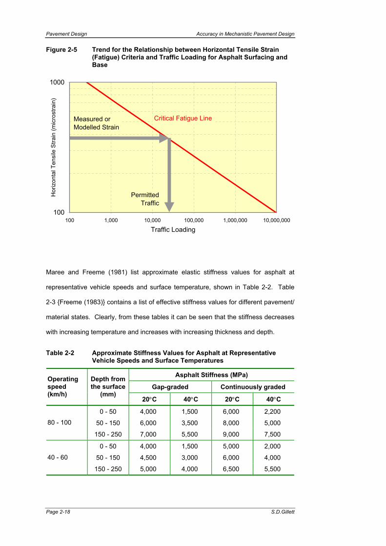
Pavement Design Accuracy in Mechanistic Pavement Design
Page 2-18 S.D.Gillett
Figure 2-5 Trend for the Relationship between Horizontal Tensile Strain (Fatigue) Criteria and Traffic Loading for Asphalt Surfacing and Base
100
1000
100 1,000 10,000 100,000 1,000,000 10,000,000
Traffic Loading
Hor
izon
tal T
ensi
le S
train
(mic
rost
rain
)
Measured orModelled Strain
PermittedTraffic
Critical Fatigue Line
Maree and Freeme (1981) list approximate elastic stiffness values for asphalt at
representative vehicle speeds and surface temperature, shown in Table 2-2. Table
2-3 {Freeme (1983)} contains a list of effective stiffness values for different pavement/
material states. Clearly, from these tables it can be seen that the stiffness decreases
with increasing temperature and increases with increasing thickness and depth.
Table 2-2 Approximate Stiffness Values for Asphalt at Representative Vehicle Speeds and Surface Temperatures
Asphalt Stiffness (MPa)
Gap-graded Continuously graded Operating speed (km/h)
Depth from the surface
(mm) 20°C 40°C 20°C 40°C
0 - 50 4,000 1,500 6,000 2,200
50 - 150 6,000 3,500 8,000 5,000 80 - 100
150 - 250 7,000 5,500 9,000 7,500
0 - 50 4,000 1,500 5,000 2,000
50 - 150 4,500 3,000 6,000 4,000 40 - 60
150 - 250 5,000 4,000 6,500 5,500

Accuracy in Mechanistic Pavement Design Pavement Design
PhD Thesis Page 2-19
Table 2-3 Approximate Stiffness Values for Varying Asphalt Mixes
Asphalt Stiffness (MPa)
Good condition or new
Stiff dry mixture
Very cracked condition
Material Grading
Depth from the surface
(mm)
20°C 40°C 20°C 40°C 20°C 40°C
0 - 50 4,000 1,500 5,000 1,800 1,000 500
50 - 150 6,000 3,500 7,000 4,000 1,000 500
Gap graded
150 - 250 7,000 5,500 8,000 6,000 1,000 500
0 - 50 6,000 2,200 7,000 4,000 750 500
50 - 150 8,000 5,500 9,000 6,000 1,000 750
Continuously graded
150 - 250 9,000 7,500 10,000 8,000 1,000 750
2.6.2 The Behaviour of Unbound Granular Bases and Subbases
Pavement layers constructed with unbound granular materials may be used in the
base, subbase and even selected layers. The characteristics of these layers will
depend on the quality of material used to construct the layer and the specifications to
which the layers are constructed. Typically, crushed rock will be used for upper layers
and natural gravel in lower layers. The characteristics of these layers depend on the
quality of parent material used to construct the layer and the specifications
(compaction) to which the layers were constructed.
Pavements that comprise base layers of untreated granular material often have a
relatively thin bituminous surface layer (40 - 100 mm), and it is in these circumstances
that the characteristics of the unbound granular material are critical to design. Most
pavements have granular subbase layers and although it is important during
construction to provide a working platform on which materials can be transported, laid
and compacted, these layers are lower in the pavement structure and thus the
stresses are reduced and their behaviour less critical.
Approximate values of the resilient moduli for granular material are given in Table 2-4
{Freeme (1983), updated by Jordaan (1993)}.

Pavement Design Accuracy in Mechanistic Pavement Design
Page 2-20 S.D.Gillett
Table 2-4 Approximate Resilient Moduli for Granular Materials at Various Moisture Conditions
Resilient Moduli (MPa) Material
Description Dry, well
compacted, good support
Dry, well compacted,
poor support
Wet, good support
Wet, poor support
High quality crushed stone
450 (250 - 1,000) 150 -600 50 - 250 40 - 200
Crushed stone 400 (200 - 800) 100 - 400 50 - 200 40 - 200
Crushed stone 350 (200 - 800) 100 - 350 50 - 150 40 - 200
Gravel base quality
300 (100 - 600) 75 - 350 50 - 150 30 - 200
Gravel 250 (50 - 400) 40 - 300 30 - 200 20 - 150
Gravel 225 (50 - 200) 30 - 200 20 - 150 20 - 150
Poisson's ratio is 0.35
Of course, there is some contention when particular values are published, such as
those shown above, since the resilient moduli are stress dependent. These values
do, however, give engineers some indication of likely magnitudes for values at likely
stress values expected in pavements under traffic loading as discussed. The table
also provides different ranges of values for different moisture conditions at different
densities and levels of support.
Of the analytical design methods discussed earlier, only the SA-MDM considered that
cumulative permanent deformation or inadequate stability in granular bases under
repetitive traffic loading might be critical. In this method both of these distress modes
have been related to the shear strength of the material {Maree and Freeme (1981)}
and therefore, by limiting the allowable shear stress in the layer, distress can be
avoided. The allowable shear stress under a single wheel load is calculated from the
maximum single load shear strength, expressed in terms of the Mohr - Coulomb
strength parameters, apparent cohesion and the angle of internal friction, and a
selected ‘Factor of Safety’ as determined from laboratory triaxial tests. The general
trend of the relationship with traffic loading is shown in Figure 2-6. This term, Factor

Accuracy in Mechanistic Pavement Design Pavement Design
PhD Thesis Page 2-21
of Safety, is somewhat misleading and a better term might be ‘Granular Load Factor’,
however Factor of Safety will be used herein to avoid confusion with the SA-MDM.
The Factor of Safety at any point in the layer has been defined {Maree (1978), Maree
(1982)} such that:
F
Strength Shear MaximumStress Shear Allowable = Eqn.2-2
Where: F Factor of Safety
It was shown by Maree that:
( )w3w1
2w3
σσ2θ45tancK21
2θ45tanKσ
F−
+××+
−
+
= Eqn.2-3
Where: c Cohesion φ Angle of internal friction K Material constant (suggested values are 0.6 for
highly saturated conditions and 0.95 for normal conditions)
σ1w & σ3w Calculated major and minor principal stresses acting at that point in the layer (allowable stresses) (with comprehensive stresses positive and tensile stresses negative)
Figure 2-6 Trend for the Relationship between Factor of Safety (Shear Strength) Criterion and Traffic Loading for Unbound Granular Materials
0.0
0.5
1.0
1.5
2.0
10,000 100,000 1,000,000 10,000,000 100,000,000Traffic Loading
Fact
or o
f Saf
ety
Measured orModelled F
Permitted Traffic9,000,000 ESA
Shear Strength Criterion

Pavement Design Accuracy in Mechanistic Pavement Design
Page 2-22 S.D.Gillett
The SA-MDM suggests that the Factor of Safety be calculated at the mid-depth of a
granular layer and at a point one sixth of the layer thickness from the bottom of the
layer of the base layer under one of the wheel loads and at a vertical line between
dual wheel loads.
2.6.3 The Behaviour of Subgrade Soils and Selected Layers
In addition to surface cracking, another principal measure of pavement behaviour is
permanent deformation. Since the early 1960s the vertical elastic strain at the top of
the subgrade soil, calculated with linear elastic theory, has been used to develop
limiting strain criteria to control permanent deformation in this layer and therefore the
rutting of the pavement {AASHO (1962); Walker et al (1977); Maree and Freeme
(1981)}. Although there is a shortcoming with this approach (notably that the
permanent plastic behaviour of pavement structures is related to resilient behaviour)
the magnitude of stress in the subgrade at formation level is strongly influenced by the
stiffness of the subgrade; moreover subgrade resilient modulus affects the level of
stresses generated in all the pavement layers constructed on top of this layer. The
resilient modulus of the subgrade is strongly influenced by moisture conditions.
A table of typical resilient moduli of subgrade materials is given Table 2-5 {Jordaan
(1993)}. Again there is some contention because fixed values are assigned to
materials whereas these materials are stress dependent.
Table 2-5 Approximate Resilient Moduli of Subgrade Materials at Different Moisture Conditions
Resilient Modulus (MPa) Material Soaked CBR
(%) Wet state Dry state
Gravel-soil <15 20 - 120 30 - 200
Gravel-soil <10 20 - 90 30 - 180
Gravel-soil <7 20 - 70 30 - 140
Gravel-soil <3 10 - 45 20 - 90
Figure 2-7 shows a typical design relationship linking resilient axial strain at the top of
the subgrade with a permissible traffic loading level.
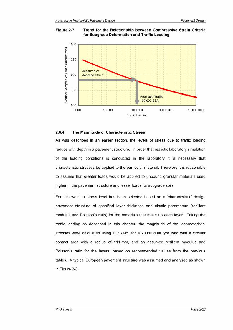
Accuracy in Mechanistic Pavement Design Pavement Design
PhD Thesis Page 2-23
Figure 2-7 Trend for the Relationship between Compressive Strain Criteria for Subgrade Deformation and Traffic Loading
500
750
1000
1250
1500
1,000 10,000 100,000 1,000,000 10,000,000
Traffic Loading
Ver
tical
Com
pres
ive
Stra
in (m
icro
stra
in)
Measured orModelled Strain
Predicted Traffic100,000 ESA
2.6.4 The Magnitude of Characteristic Stress
As was described in an earlier section, the levels of stress due to traffic loading
reduce with depth in a pavement structure. In order that realistic laboratory simulation
of the loading conditions is conducted in the laboratory it is necessary that
characteristic stresses be applied to the particular material. Therefore it is reasonable
to assume that greater loads would be applied to unbound granular materials used
higher in the pavement structure and lesser loads for subgrade soils.
For this work, a stress level has been selected based on a ‘characteristic’ design
pavement structure of specified layer thickness and elastic parameters (resilient
modulus and Poisson’s ratio) for the materials that make up each layer. Taking the
traffic loading as described in this chapter, the magnitude of the ‘characteristic’
stresses were calculated using ELSYM5, for a 20 kN dual tyre load with a circular
contact area with a radius of 111 mm, and an assumed resilient modulus and
Poisson’s ratio for the layers, based on recommended values from the previous
tables. A typical European pavement structure was assumed and analysed as shown
in Figure 2-8.

Pavement Design Accuracy in Mechanistic Pavement Design
Page 2-24 S.D.Gillett
Figure 2-8 Materials and Pavement Details for the Calculation of Characteristic Stresses
Asphalt 150 mm Point of AnalysisE1 4,000 MPa Bottom of the Surface Layerv1 0.44 Depth=
Point of AnalysisGranular Base 300 mm Centre of the Base Layer
E2 450 MPa Depth=v2 0.35
Point of AnalysisGranular Subbase 300 mm Centre of the Subbase Layer
E2 200 MPa Depth=v2 0.35
Point of AnalysisSel.Subgrade Soil 1000 mm Top of the Sel.Subgrade Layer
E3 100 MPa Depth=v3 0.35
Point of AnalysisSubgrade Soil Infinite Depth Top of the Subgrade Layer
E3 50 MPa Depth=v3 0.35
- Analysis Point
600 mm
751 mm
1751 mm
149 mm
300 mm
Wheel Load Wheel Load520 kPa 520 kPa
It is recognised that the material parametric values (resilient modulus and Poisson’s
ratio) obtained from this first analysis should be re-entered and the pavement re-
analysed using ELSYM5 with the new parameters and so on until an insignificant
change in the parameters between this analysis and the previous analysis is obtained.
This analysis was conducted and although the Resilient Modulus and Poisson’s ratio
varied somewhat, as shown graphically in Figure 2-9, the characteristic stresses in the
base and the subgrade only varied by approximately 4 kPa between the initial iteration
and the last. As a consequence of this, and the fact that the characteristic stresses
are somewhat arbitrary anyway, the initial values were used for characterisation of
materials and pavements in this work.
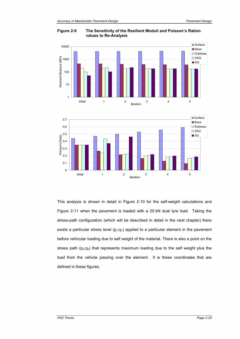
Accuracy in Mechanistic Pavement Design Pavement Design
PhD Thesis Page 2-25
Figure 2-9 The Sensitivity of the Resilient Moduli and Poisson’s Ration values to Re-Analysis
1
10
100
1000
10000
Initial 1 2 3 4 5Iteration
Res
ilien
t Mod
ulus
(MP
a)
SurfaceBaseSubbaseSSGSG
0
0.1
0.2
0.3
0.4
0.5
0.6
0.7
Initial 1 2 3 4 5Iteration
Poi
sson
's R
atio
SurfaceBaseSubbaseSSGSG
This analysis is shown in detail in Figure 2-10 for the self-weight calculations and
Figure 2-11 when the pavement is loaded with a 20 kN dual tyre load. Taking the
stress-path configuration (which will be described in detail in the next chapter) there
exists a particular stress level (p1;q1) applied to a particular element in the pavement
before vehicular loading due to self weight of the material. There is also a point on the
stress path (p2;q2) that represents maximum loading due to the self weight plus the
load from the vehicle passing over the element. It is these coordinates that are
defined in these figures.

Pavement Design Accuracy in Mechanistic Pavement Design
Page 2-26 S.D.Gillett
Figure 2-10 The Self Weight Characteristic Stress within a Typical European Pavement Structure
Self Weight Characteristics: 5-Layer StructureMean Deviator
q1 =Bottom of the Asphalt: 2 kPa
Centre of the Granular Base: 3 kPaCentre of the Granular Subbase: 7 kPa
Top of the Selected Subgrade: 8 kPaTop of the Subgrade: 17 kPa
Compresive stress is positiveIn the Pavement Structure Anisotropy - Ratio σ1:σ3 2 : 1
Peak Deflection on the SurfaceStress - Bottom of the Surface Layer σ1(kPa) σ2(kPa) σ3(kPa)Depth= 149 mm 3 2 2Stress - Centre of the Base Layer σ1(kPa) σ2(kPa) σ3(kPa)Depth= 300 mm 7 3 3Stress - Centre of the Subbase Layer σ1(kPa) σ2(kPa) σ3(kPa)Depth= 600 mm 13 7 7Stress - Top of the Selected Subgrade Layer σ1(kPa) σ2(kPa) σ3(kPa)Depth= 751 mm 16 8 8Stress - Top of the Subgrade Layer σ1(kPa) σ2(kPa) σ3(kPa)Depth= 1751 mm 34 17 17
11 kPa
2 kPa5 kPa9 kPa
p1 =
23 kPa
4 1000
1
5 Inf.
150
2 300
3 300
Based on this analysis characteristic stresses that are typically applied to an unbound
granular base and subbase and those typically applied to a subgrade soil are
calculated and are shown in red in Table 2-6. These stresses can be defined as the
independent variables for which the elastic parameters (dependent variables) for the
materials are calculated. This will allow a comparison to be made between materials
and specimens since the same stresses will be applied.
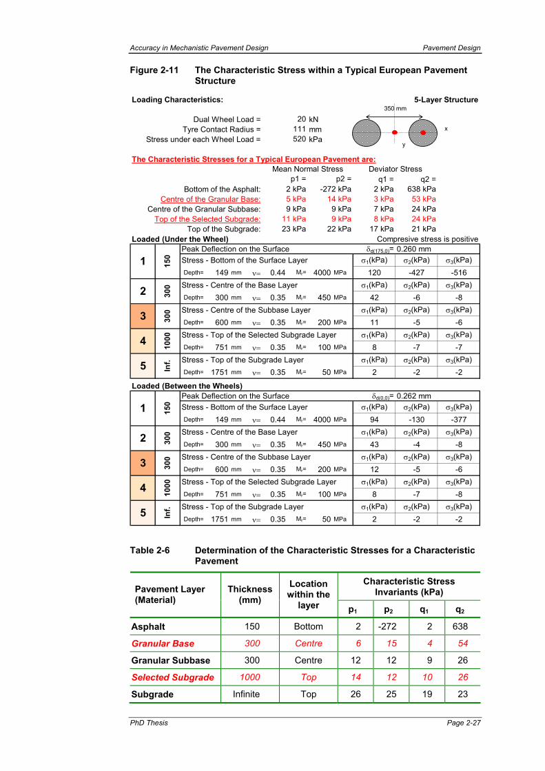
Accuracy in Mechanistic Pavement Design Pavement Design
PhD Thesis Page 2-27
Figure 2-11 The Characteristic Stress within a Typical European Pavement Structure
Loading Characteristics: 5-Layer Structure
Dual Wheel Load = kNTyre Contact Radius = mm
Stress under each Wheel Load = kPa
The Characteristic Stresses for a Typical European Pavement are:
q1 = q2 =Bottom of the Asphalt: 2 kPa 638 kPa
Centre of the Granular Base: 3 kPa 53 kPaCentre of the Granular Subbase: 7 kPa 24 kPa
Top of the Selected Subgrade: 8 kPa 24 kPaTop of the Subgrade: 17 kPa 21 kPa
Loaded (Under the Wheel) Compresive stress is positivePeak Deflection on the Surface δd(175,0)= 0.260 mmStress - Bottom of the Surface Layer σ1(kPa) σ2(kPa) σ3(kPa)Depth= 149 mm ν= 0.44 Mr= 4000 MPa 120 -427 -516Stress - Centre of the Base Layer σ1(kPa) σ2(kPa) σ3(kPa)Depth= 300 mm ν= 0.35 Mr= 450 MPa 42 -6 -8Stress - Centre of the Subbase Layer σ1(kPa) σ2(kPa) σ3(kPa)Depth= 600 mm ν= 0.35 Mr= 200 MPa 11 -5 -6Stress - Top of the Selected Subgrade Layer σ1(kPa) σ2(kPa) σ3(kPa)Depth= 751 mm ν= 0.35 Mr= 100 MPa 8 -7 -7Stress - Top of the Subgrade Layer σ1(kPa) σ2(kPa) σ3(kPa)Depth= 1751 mm ν= 0.35 Mr= 50 MPa 2 -2 -2
Loaded (Between the Wheels)Peak Deflection on the Surface δd(0,0)= 0.262 mmStress - Bottom of the Surface Layer σ1(kPa) σ2(kPa) σ3(kPa)Depth= 149 mm ν= 0.44 Mr= 4000 MPa 94 -130 -377Stress - Centre of the Base Layer σ1(kPa) σ2(kPa) σ3(kPa)Depth= 300 mm ν= 0.35 Mr= 450 MPa 43 -4 -8Stress - Centre of the Subbase Layer σ1(kPa) σ2(kPa) σ3(kPa)Depth= 600 mm ν= 0.35 Mr= 200 MPa 12 -5 -6Stress - Top of the Selected Subgrade Layer σ1(kPa) σ2(kPa) σ3(kPa)Depth= 751 mm ν= 0.35 Mr= 100 MPa 8 -7 -8Stress - Top of the Subgrade Layer σ1(kPa) σ2(kPa) σ3(kPa)Depth= 1751 mm ν= 0.35 Mr= 50 MPa 2 -2 -2
1000
Inf.
4
20111520
Mean Normal Stress
3
p1 =15
030
0Deviator Stress
9 kPa22 kPa
p2 =-272 kPa
14 kPa9 kPa
5 Inf.
300
150
1000
1
2 kPa5 kPa9 kPa
1
11 kPa23 kPa
2 300
5
2 300
3
4
350 mm
y
x
Table 2-6 Determination of the Characteristic Stresses for a Characteristic Pavement
Characteristic Stress Invariants (kPa) Pavement Layer
(Material) Thickness
(mm)
Location within the
layer p1 p2 q1 q2
Asphalt 150 Bottom 2 -272 2 638
Granular Base 300 Centre 6 15 4 54
Granular Subbase 300 Centre 12 12 9 26
Selected Subgrade 1000 Top 14 12 10 26
Subgrade Infinite Top 26 25 19 23

Pavement Design Accuracy in Mechanistic Pavement Design
Page 2-28 S.D.Gillett
2.7 SUMMARY
The benefits of implementing mechanistic, as opposed to empirical, design
procedures for new pavement construction, reconstruction, or rehabilitation are many.
The key benefit is in providing the designer with powerful tools to evaluate the
performance (specific distress types) of different pavement designs, instead of relying
solely on limited empirical correlations or opinions.
A number of different pavement design factors such as material quality, moisture
conditions and layer thickness can be examined using an analytical or mechanistic
design approach giving these methods the potential to improve pavement design and
to provide more reliability to designs.
It is recognised that laboratory tests that seek to simulate conditions in the road
pavement are gross simplifications. Some correlation is possible from empirical
laboratory test results to the elastic parameters required for analytical pavement
design, however these correlations are inadequate. Laboratory tests have been
developed using more sophisticated apparatus such as repeated load triaxial, hollow
cylinder, shear box or simple shear tests, however there is some reluctance by
engineers to change from the relatively inexpensive simple characterisation tests
described above to the complexity of non-standard material testing. These complex
test procedures are almost exclusively used for research purposes although the
repeated load triaxial test is becoming the test most widely used for determination of
resilient and permanent strain properties of road construction materials and
international standards are being compiled for its commercial use.
The performance testing of full-scale pavements, ideally under controlled conditions of
wheel load, moisture, climate and temperature, play an essential part in the
development and calibration of the analytical pavement design. Pavement designs
that are based on the parameters obtained from laboratory testing and the consequent
analytical design methods require practical verification over a long term in the field.
When comparing the results obtained from laboratory tests conducted on material
specimens it is convenient to have some numeric parameter value. In order to use

Accuracy in Mechanistic Pavement Design Pavement Design
PhD Thesis Page 2-29
the resilient modulus or Poisson’s ratio some arbitrary stress conditions must be
defined. These are taken as representative stress levels as would be experienced in
a ‘typical’ pavement structure. These stresses are defines as ‘characteristic stresses’,
for which the characteristic elastic parameters for a particular material can be
determined.
The number of flexible pavement design methods that make direct use of mechanistic
design procedures is increasing. All of these design methods have developed
procedures for the general application to a variety of design considerations, however
most of these design methods are primarily concerned with the two critical strains
values namely the:
• Horizontal tensile strain at the bottom of the asphalt layer (to limit asphalt
fatigue cracking), and;
• Vertical compressive strain at the top of the subgrade (to prevent excessive
permanent deformation).
Of the design methods investigated the only method that presented a means of
assessing the shear deformation and failure in the unbound granular layers for
pavements with thin asphalt surfaces (40 – 60 mm) constructed on granular bases
was the SA-MDM, which is therefore used here.
Of course, once validated for particular circumstances the parameters (allowable
strains) and consequent designs will vary between locations due to climate,
topography, material quality, etc.


Accuracy in Mechanistic Pavement Design Pavements Materials
PhD Thesis Page 3-1
3 STRESSES AND STRAINS IN ROAD PAVEMENT MATERIALS
3.1 INTRODUCTION
Pavement materials, such as unbound granular aggregate layers and soil subgrades,
that make up the layers of a pavement structure exhibit two distinct types of behaviour
when placed under the traffic loads:
• Elastic behaviour, which determines the load spreading ability of the layer, which
manifests as cracking due to fatigue of the upper layers, and;
• Permanent deformation, which causes a build up of irrecoverable deformation,
which after a number of load applications becomes apparent as rutting.
Consider a cylindrical element in a pavement as shown in Figure 3-1. As a vehicle
passes over the cylindrical element a stress pulse is applied to it. These stress pulses
are applied repeatedly in large numbers for the duration of the life of the pavement.
For simplicity, it is assumed that each successive load is of equal magnitude.
However, because this is not the case, an equivalency technique is used to reduce
the actual or likely spectrum of applied loads to an ‘equivalent’ number of loads of a
fixed magnitude (See Section 3.2.2).
The cylindrical element will also experience a constant stress due to the overburden
pressure of the material above it.
The element will deform in both the axial and radial direction with each stress pulse.
As shown in Figure 3-1 the elastic deformation recovers after each load. There is,
however, there is a small permanent deformation applied to the element at each load
cycle.
At an increasing number of load repetitions, the deformation of the material becomes
almost entirely recoverable. The diminishing accumulating non-recoverable
deformation from each of the stress applications is the permanent deformation {Thom
(1988)}.
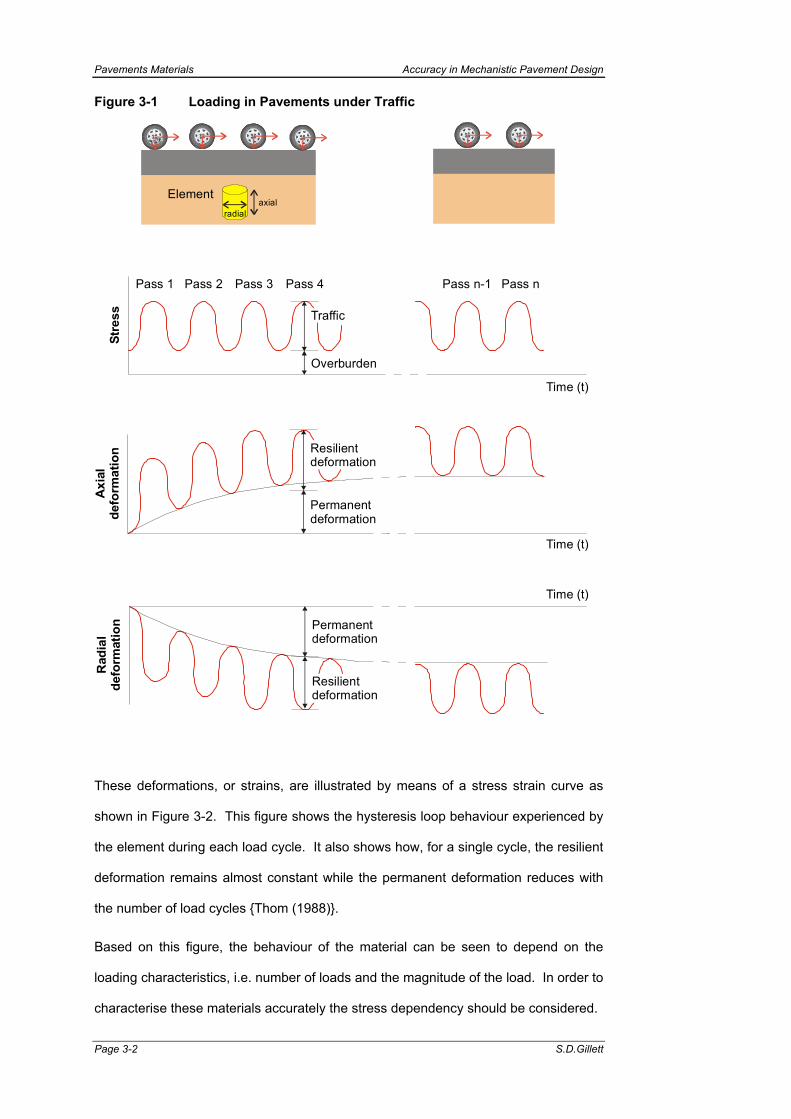
Pavements Materials Accuracy in Mechanistic Pavement Design
Page 3-2 S.D.Gillett
Figure 3-1 Loading in Pavements under Traffic
Elementradial
axial
Rad
ial
defo
rmat
ion
Pass 1 Pass 2 Pass 3 Pass 4
Stre
ss
Overburden
Time (t)
Traffic
Permanentdeformation
Axi
alde
form
atio
n
Permanentdeformation
Resilientdeformation
Time (t)
Time (t)
Pass n
Resilientdeformation
Pass n-1
These deformations, or strains, are illustrated by means of a stress strain curve as
shown in Figure 3-2. This figure shows the hysteresis loop behaviour experienced by
the element during each load cycle. It also shows how, for a single cycle, the resilient
deformation remains almost constant while the permanent deformation reduces with
the number of load cycles {Thom (1988)}.
Based on this figure, the behaviour of the material can be seen to depend on the
loading characteristics, i.e. number of loads and the magnitude of the load. In order to
characterise these materials accurately the stress dependency should be considered.
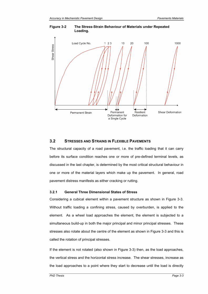
Accuracy in Mechanistic Pavement Design Pavements Materials
PhD Thesis Page 3-3
Figure 3-2 The Stress-Strain Behaviour of Materials under Repeated Loading.
3.2 STRESSES AND STRAINS IN FLEXIBLE PAVEMENTS
The structural capacity of a road pavement, i.e. the traffic loading that it can carry
before its surface condition reaches one or more of pre-defined terminal levels, as
discussed in the last chapter, is determined by the most critical structural behaviour in
one or more of the material layers which make up the pavement. In general, road
pavement distress manifests as either cracking or rutting.
3.2.1 General Three Dimensional States of Stress
Considering a cubical element within a pavement structure as shown in Figure 3-3.
Without traffic loading a confining stress, caused by overburden, is applied to the
element. As a wheel load approaches the element, the element is subjected to a
simultaneous build-up in both the major principal and minor principal stresses. These
stresses also rotate about the centre of the element as shown in Figure 3-3 and this is
called the rotation of principal stresses.
If the element is not rotated (also shown in Figure 3-3) then, as the load approaches,
the vertical stress and the horizontal stress increase. The shear stresses, increase as
the load approaches to a point where they start to decrease until the load is directly

Pavements Materials Accuracy in Mechanistic Pavement Design
Page 3-4 S.D.Gillett
above the particular element at which point there is no shear stress on vertical and
horizontal planes. This is when pure triaxial conditions exist. As the load moves away
a complete reversal of shear stress occurs, this too is shown in Figure 3-3.
Unfortunately, as discussed later, these stress rotation effects cannot be duplicated in
the repeated load triaxial apparatus and this is therefore a limitation of this apparatus.
Figure 3-3 Loading of an Element in a Pavement Showing the Rotation of the Principal Stresses.
Principal Stresses Normal Stresses
3.2.2 Vehicular Loading Characteristics
Wheeled vehicular loading causes cyclic stresses to be applied to the pavement
structure. These are generally in the form of a large number of rapidly applied stress
pulses of varying magnitude. For pavement design purposes it is necessary not only
to consider the total number of wheel loads but also the magnitude of individual loads,
their duration and the frequency of loading repetition.
Loading Magnitude
Each wheel load will be of a different magnitude. Since the damage caused by each
wheel passage on the pavement depends strongly on this magnitude it is convenient,
and practically necessary, to equate the applied wheel loads over the life of the road
pavement to an equivalent number of standard wheel loads that would cause the
same damage {Paterson (1987)}. This is achieved by expressing the cumulative load
in terms of Equivalent Standard Axles (ESA). Where it is desirable to express
pavement life in terms of years, rather than ESAs, it is common to relate the traffic

Accuracy in Mechanistic Pavement Design Pavements Materials
PhD Thesis Page 3-5
pattern expected to the ESAs that they will produce by classifying the vehicles into
various groups each with a set number of ESAs per vehicle.
Most pavement designs are based on a standard 80 kN axle load comprising four
tyres, two on each side of the axle. Some computer analysis programs allow the
application of multiple loads and this actual configuration can be used, unfortunately
however, some computer programs only allow for a single load. Consequently, two
different load configurations are used in this work, for the analytical procedures, each
applying the same pressure to the road surface as defined in Figure 3-4.
Figure 3-4 Pavement Loading Characteristics
Load on the Wheel = 40 kN
Pressure from the Wheel = 520 kPa
R =156 mm
Load on each Wheel = 20 kNPressure from each Wheel = 520 kPa
R =111 mm
165 mm
165 mm
R =111 mm
Load Duration and the Frequency of Loading Repetition
The duration of the load in a road pavement has been investigated {Barksdale
(1971)}. The time at which a vertical stress pulse is applied to a pavement, for
different vehicle speeds at different depths, is shown in Figure 3-5.
The frequency of loading repetition is controlled by the speed at which vehicles travel
on the road, the type of vehicle using the road and the number of vehicles on the road.
Therefore in order to simulate traffic moving over a pavement surface, it is necessary
to apply a large number of rapidly applied stress pulses. For moderate vehicle

Pavements Materials Accuracy in Mechanistic Pavement Design
Page 3-6 S.D.Gillett
speeds, the stress pulse lasts between about 0.02 and 0.2 sec. The pulse time
increases with increasing depth in the pavement and decreasing vehicle speed.
Figure 3-5 Vertical Stress Pulse Time as a Function of the Depth in a Pavement for different Vehicle Speeds
Vehicle speed (v)
v = 2 km/h
v = 25 km/h
v = 50 km/h
v = 70 km/h
10
1.0
0.2
0.1
0.05
0.03
0.01
0.022
0.034
0.067
0.900
0 100 200 300 400 500 600 700
Depth beneath pavement surface (mm)
Equi
vale
nt v
ertic
al s
tress
pul
se ti
me
(s)
0.02
After Barksdale (1971)
The vehicle speed determines the rate of loading. For this reason vehicle speed
needs to be taken when considering the properties of bituminous mixtures due to their
visco-elastic behaviour. The rate of loading, therefore, directly affects the vertical
deflection under loading. Other materials, such as fine-grained soils, may also be
sensitive to rate of loading although to a lesser extent, but these are usually located
so deep in the pavement that the vehicle speed has a relative minor effect on their
properties.
It was shown by Barksdale et al.(1990) that near the surface the stress pulse has a
pronounced haversine shape and with depth the pulse duration becomes greater and,
although it remains haversine in shape, a triangular loading gives a reasonably good
approximation.

Accuracy in Mechanistic Pavement Design Pavements Materials
PhD Thesis Page 3-7
3.3 THE BEHAVIOUR OF PAVEMENT MATERIALS UNDER TRAFFIC LOADING
A better understanding of the behaviour of the materials that are used for road
construction will allow materials to be used more economically and with more
environmental acceptance. This detailed understanding will enable more relevant
specifications to be compiled rather than those defined by the present empirical
specifications.
3.3.1 Subgrade Soils
With regard to fine grained soils, or soils whose behaviour depends on the fine
fraction there is limited knowledge on the quantitative influence on mechanical
properties of:
• The water content, which results from environmental and drainage conditions;
• The stress history of the soil, this is especially the case for re-compacted soils
which form the pavement’s foundation as embankments (and probably
elsewhere).
Such influences are not rationally accounted for in empirical design methods.
Previous work on soils has indicated that the elastic parameters of soils are influenced
by a number of variables {Seed at al (1955), Hyde (1974), Loach (1987)}. These
include not only the physical conditions such as the stress state, moisture content,
and the pre-consolidation pressure but also such variables as the rate of loading and
number of load applications.
The stress-strain response of soils is known to be non-linear. The sensitivity of the life
of a pavement to changes in the value of Young’s Modulus of the subgrade was
demonstrated by Hight and Stevens (1982) and thus there is a clear need to
accurately estimate the modulus of the subgrade at the design stage. The elastic
properties are needed so that the resilient modulus of the foundation under
construction or under normal traffic loading can be computed and an appropriate
design of the placed layers, especially the bound layers, undertaken.

Pavements Materials Accuracy in Mechanistic Pavement Design
Page 3-8 S.D.Gillett
Conventionally, subgrades are characterised by a CBR, either determined in-situ or in
the laboratory. As discussed in the previous chapter, this is an empirical penetration
test (principally inducing failure) and is not of direct use in an analytical design
method, which requires a stress-strain model. A further difficulty is the need to test
the soil at those stresses, water and suction conditions that may pertain during the life
of the pavement, a condition that may differ from those at the time of design.
These different conditions can be controlled and varied during a repeated load triaxial
test. The resilient and permanent strains resulting from different repeated stress
paths and different states of initial suction in soils was a principal area of study of the
‘Science Project’ on which this thesis draws. For the work in this thesis material
characteristics such as moisture content and stress application values were chosen
as close to the actual values found in road pavements in Europe as was possible.
Since these materials are fine grained, small specimens can be tested thus allowing
more conventional triaxial apparatus to be modified for repeated load testing.
3.3.2 Unbound Granular Materials
In recent years much work has been done on the investigation of the behavioural
properties of unbound granular materials and subgrade soils in pavement structures
under traffic loading {Sweere (1990), Boyce (1976), Pappin (1979)}. Unbound
granular materials generally make up the subbase layers of roads and may be used in
base layers of relatively lightly trafficked roads. These materials are generally
characterised by their resistance to impact, for example Los Angeles Abrasion value,
and their geological characterisation. This means that marginal materials that might
have been satisfactory for construction as well as being cheaper are often excluded
by specifications. Since these granular materials are usually found higher in the
pavement they are subjected to higher levels of stress and more markedly rotating
stresses. For this reason more detailed characterisation by advanced test methods
may be more important than for the materials found lower down in the pavement
structure (subgrade soils).

Accuracy in Mechanistic Pavement Design Pavements Materials
PhD Thesis Page 3-9
Some research has been conducted {Cheung (1994)} to find an inexpensive simple
test that allows these materials to be characterised with respect to their stress-strain
response, but it appears that the repeated load triaxial test remains the most
appropriate test method.
For the study of full sized aggregates used in road pavements, railway ballast or other
engineering applications, such as earthquake problems, where repeated loading
occurs, the specimen size must be large enough so as not to have an influence on the
behaviour of the material. A general rule of thumb is that the diameter of the specimen
should be not less than ten times the largest particle size, although often seven is
used. Thus for road aggregates of 0/40 mm grading a specimen diameter of about
300 mm is required.
3.4 REPEATED LOAD TRIAXIAL TESTING
The principle of repeated load triaxial tests is to simulate an element in a pavement by
manufacturing a specimen of road construction material and applying similar load
conditions to those that might be experienced in the field while measuring the
deformation experienced by the specimen. The purpose of the test is to determine the
material parameters under simulated traffic loading conditions, such as resilient strain
parameters and permanent strain parameters. Due to the stress dependent
behaviour of these unbound materials the elastic parameters must be determined at a
number of stress levels.
A solid cylindrical specimen is formed by compacting material into a steel mould at a
predefined moisture content and density. The specimen is placed on top of a rigid
bottom platen and a second rigid platen is then placed on top of the specimen. The
specimen is sealed against the platens by enclosing it within a rubber membrane.
The specimen is then either placed in a cell where an all-round confining stress is
applied to the specimen or the confining pressure is applied by means of a partial
vacuum within the membrane. This confining pressure simulates the lateral stress
caused by the overburden pressure. An axial load through the platens simulates the
applied wheel loadings.

Pavements Materials Accuracy in Mechanistic Pavement Design
Page 3-10 S.D.Gillett
The triaxial compression test has been used as the basic testing apparatus in
geotechnical engineering to evaluate stiffness and shear strength of cohesive and
granular materials. The early pioneering work performed by Seed et al (1955); Seed
and Fead (1959), and Seed at al (1962) was all conducted using the repeated load
triaxial test apparatus. This apparatus was first developed from the monotonic load
triaxial test by incorporating loading systems that could simply apply and remove the
deviator stress, while the confining stress was kept constant. However, Allen and
Thompson (1974) reported going one step further by applying not only a repeated
deviator stress, but also a repeated confining stress. These Variable Confining
Pressure (VCP) tests are a closer simulation of actual field conditions than the
Constant Confining Pressure (CCP) tests, since in the road structure the confining
stress acting on the material is repeated as a load approaches.
Today the repeated load triaxial compression test is by far the most commonly used
method to evaluate the resilient modulus for pavement design and research purposes
{Barksdale et al (1990)}.
3.4.1 Repeated Load Triaxial Apparatus Configurations
There are basically three different methods, and corresponding apparatus, with which
one can conduct repeated load triaxial tests on road construction materials. These
different configurations are shown schematically in Figure 3-6 and illustrated in
Photograph 3-1 and are as follows:
• Conventional repeated load triaxial test, with constant confining pressure.
• Internal vacuum repeated load triaxial test, with constant confining pressure.
• Variable confining pressure repeated load triaxial test.
Conventional Repeated Load Triaxial Test
The cylindrical specimen is placed inside a triaxial cell on top of a rigid bottom platen,
a rigid platen is placed on top of the specimen, and a rubber membrane is placed
around the specimen. A cylindrical chamber is placed around the specimen. The
specimen is subjected to a constant confining pressure by increasing the pressure
within the chamber. Drainage lines lead to porous stones located in the top and

Accuracy in Mechanistic Pavement Design Pavements Materials
PhD Thesis Page 3-11
bottom platens and atmospheric pressure can be maintained within the specimen by
leaving these lines open. By keeping the pressure inside the specimen at
atmospheric pressure the confining pressure applied to the specimen is equal to the
pressure applied within the cell (measured relative to atmospheric pressure). A
repeated axial load is applied to the ends of the specimen by way of the platens
simulating traffic loading.
Figure 3-6 Schematic Illustration of the Repeated Load Triaxial Apparatus
Spe
cimen
Spe
cimen
Drainage
Dr ainageDrainage
Drainage
Drainag e
Vacuum
Vacuum
CellCell
Conventional repeatedload triaxial test.
Vacuum method ofrepeated loadtriaxial test.
Var iable confiningpres sure repeatedload triaxial test.
Spec
imen
R R
R R
Spe
cim
en
Mem
bran
e
Mem
bran
e
Mem
bran
e
X
X
R
R
Photograph 3-1 Repeated Load Triaxial Apparatus
Conventional repeated load triaxial apparatus
Vacuum method of repeated load triaxial method
Variable confining pressure repeated load triaxial method

Pavements Materials Accuracy in Mechanistic Pavement Design
Page 3-12 S.D.Gillett
Vacuum Method Repeated Load Triaxial Test
This test is similar to the conventional test except that, instead of the confining
pressure being applied by fluid within a cell surrounding the specimen, the confining
pressure is supplied by means of a partial vacuum inside the membrane. This method
is used on big specimens of granular material where, due to the size of the specimen,
the cell would be impracticably large. Again, a repeated axial load is applied to the
ends of the specimen simulating traffic loading.
Variable Confining Pressure Repeated Load Triaxial Test
In reality, the lateral pressure on an element of material in a pavement builds up as
vehicles approach and decreases as they move away. Thus it is desirable to vary the
confining pressure by using fluid in the cell controlled by a fairly sophisticated
electronic control system. A repeated load is applied axially as above and
simultaneously a repeated confining load is applied to the specimen via the fluid.
These loads are independent of one another and therefore many stress regimes may
be applied.
The repeated triaxial test offers four very important advantages in the investigation of
the elastic properties of materials:
1. Stress state Known principal stresses are applied to the specimen in
known directions. Thus the stress conditions within the
specimen on any plane are also known throughout the test.
2. Strain measurements
Axial and radial and thus volumetric and shear strains can be
measured and the permanent and resilient deformation
calculated. Young’s modulus (or resilient modulus) Poison’s
ratio and the bulk and shear moduli can be determined.
3. Suction measurements
Pore pressures can be easily measured at the ends of the
specimen or, with more difficulty, within the specimen.
4. Specimen drainage
The triaxial test allows relatively simple, controlled drainage
of the specimen in the axial and radial directions.

Accuracy in Mechanistic Pavement Design Pavements Materials
PhD Thesis Page 3-13
The most significant disadvantage of the triaxial cell is its limited ability to simulate the
rotation of the principal stress axes and the shear stress reversal. Only fixed
orthogonal rotation of principal stress axes are possible in this test. Also, the
intermediate principal stress applied to a specimen cannot be independently
controlled in the triaxial test.
3.4.2 Variable Confining Pressure versus Constant Confining Pressure
Although the introduction of VCP has improved the accuracy of the simulation of the
actual loading in the pavements, this has resulted in the test apparatus becoming
more complex and thus more prone to errors. However, the advent of cheaper
sophisticated electronic control equipment is easing the complexity somewhat.
Allen and Thompson (1974) investigated the influence of repeating the confining
pressure on the elastic parameters (resilient modulus and Poisson's ratio) of granular
materials. They compared variable and constant confining pressure test results on
similar specimens and reported that higher values were obtained for the elastic
parameters in the CCP tests those in the VCP tests.
Brown and Hyde (1975) later showed that two different confining pressure tests
yielded the same resilient modulus values, provided the confining stress in the CCP
test was equal to the mean value of confining stress in the VCP test. Since Allen and
Thompson had used the peak value from their VCP tests in their CCP tests, the higher
values for resilient modulus found in the CCP tests were concluded to be attributable
to the higher stress level in the test material.
Where the VCP and CCP tests yielded the same resilient modulus values, Brown and
Hyde (1975) showed that the Poisson's ratio in the CCP test differed considerably
from those obtained in VCP tests. The stress dependency of Poisson's ratio found in
the two types of tests was completely opposite. VCP tests yielded decreasing
Poisson's ratio values for increasing ratios of deviator stress over confining stress,
whereas in CCP tests Poisson's ratio was found to increase with increasing stress
ratio. Values of Poisson's ratio over 0.5 were found in the CCP tests, thereby
indicating resilient specimen dilation or volume increase.

Pavements Materials Accuracy in Mechanistic Pavement Design
Page 3-14 S.D.Gillett
Using a more fundamental approach to stress strain relationships, Brown and Hyde
(1975) showed that the problem of deviating values for Poisson's ratio found in VCP
and CCP tests can be circumvented. Separating stresses and strains into volumetric
and shear components, they showed that VCP and CCP tests do yield the same
stress strain relationships for those stress ratios that do not cause specimen dilation.
The separation of stresses and strains into volumetric and shear components will be
discussed in more detail in a forthcoming chapter. Brown and Hyde obtained a
reasonable correlation between VCP and CCP tests with respect to permanent strain
again, by setting the confining stress in the CCP tests at the mean value of confining
stress in the VCP tests.
The confinement method is largely dependent on the material particle size. Since
crushed rock granular bases comprise coarse particles of up to 40 mm, strictly, these
materials require large specimens of up to 400 mm in diameter and 800 mm in height.
Sweere (1990) stated that it is impractical to construct apparatus with confining cells
that can accommodate such large specimens and concluded that CCP tests are
adequate for determining material parameters for granular materials provided the
appropriate models are used to relate strains to stresses.
3.4.3 Apparatus Produced Factors that Influence the Triaxial Test Results
The elastic parameters of unbound materials are particularly sensitive to the testing
equipment used and the test procedure {Barksdale et al (1990)}. Therefore, particular
attention must be paid to equipment and procedure details in order to obtain reliable
values for the elastic parameters of the materials.
Specimen Alignment
Errors due to poor alignment of the specimen in the apparatus, causing the axis of the
applied load not to coincide with the axis of the specimen, have been shown to result
in seriously erroneous results {Moore et al (1970)}. Misalignment will induce
specimen ‘bending’ causing non-uniform load distribution and consequent non-
uniform strain on different sides of a specimen. Similar erroneous stresses in the
specimen are found as a consequence of the ends of a triaxial specimen not being
perpendicular to the long axis of the cylindrical specimen. To minimize misalignment

Accuracy in Mechanistic Pavement Design Pavements Materials
PhD Thesis Page 3-15
errors the triaxial cell must be carefully machined to be in perfect alignment, the cell
must be aligned relative to the external loading ram, the specimen must be a right
circular cylinder and the specimen must be aligned with the triaxial cell.
Seating Errors and Bedding Errors
Seating errors are unwanted deformations that occur when two surfaces of the testing
apparatus do not marry up perfectly against one another. Seating errors occur at a
number of critical places within the apparatus such as the connection between the
load ram and the top load platen, between the bottom platen and the base of the
triaxial cell, and between the loading platens and the porous stones.
During the manufacture of specimens and their installation into the apparatus small
irregularities exist between the ends of the specimen and the apparatus platens. As a
result of this non-uniform contact, unwanted deformation occurs in the vicinity of the
specimen ends. Many researchers have reported the seriousness of bedding errors
{Baladi et al (1988); Clayton and Khatrush (1987); Burland and Symes (1982)},
although Burland and Symes state that bedding errors are really only significant in
static tests at low deviator stress levels. During repeated load triaxial tests bedding
errors are assumed to be insignificantly small, provided that an application of load
cycles during the preconditioning phase is made.
However, it has been shown that seating and bedding errors may still be present after
preconditioning. Pezo et al (1991) reported that strong contact between the specimen
and top and bottom platens is very important. Poor seating of the platens may
introduce about 20% error in resilient modulus determination. Pezo et al (1991) used
hydrostone paste between the test specimen and the end caps, which provided
uniform contact between the specimen and caps thus eliminating some of the error in
measuring sample deformations.
End Friction or Restraint
End friction is due to the friction between the specimen end and the end platen. It can
never be completely eliminated and can result in the specimen assuming a barrel
shape when loaded. This causes a non-uniform strain distribution down the axis of
the specimen. Early static tests by Rowe and Barden (1964) show that polished end

Pavements Materials Accuracy in Mechanistic Pavement Design
Page 3-16 S.D.Gillett
platens coated with silicone grease and the insertion of a latex rubber disk between
the specimen and the end platens help to minimise friction. Boyce (1976) concluded
that better performance is obtained by replacing the rubber disc by a stainless steel
disc cut into numerous segments. He showed that during repeated load tests
performed on granular material barrelling did not occur when using frictionless ends.
Barrelling of the specimen concentrates the lateral strain in the middle {Boyce (1976)}.
Therefore greater deformation would be measured at the middle of the specimen
rather than the ends and this must be considered when applying measurement
apparatus to the specimens. Dehlen (1969) concluded, however, end friction is not
too important in resilient modulus testing provided the specimen height to diameter
ratio is at least two.
It has been reported that the most successful method of reducing end friction is to use
high vacuum silicone grease on polished steel end platens with a rubber membrane
separating the soil and grease {Lee (1976), Brown (1974), Overy (1982)}. However,
because some end restraint will always be present, the measured pore pressure will
not be exactly correct. In order to minimise this error Sangrey et al (1969) applied
very low frequencies of loading, which allow time for pore pressure equalisation.
While Koutsoftas (1978) allowed time after faster cyclic loading for the pore pressure
to equalise. In either case, the end effects will distort the recorded pore pressure but
the second method has the advantage of testing at representative frequencies or rates
of loading. Loach (1987), testing subgrade soils, stated that the most accurate pore
pressure measurements would be from a centre probe in the relatively uniform central
section of the sample before pore pressure equalisation has taken place.
System Compliance
When axial deformations are measured outside of the triaxial cell, they include both
the deformation of the specimen as well as all other deformations that occur between
the point where deformation is measured and the fixed reference point that does not
move. System compliance is the deformation that occurs within various parts of the
triaxial cell, load cell, and support system. Compliance is present in all components of
the apparatus, particularly internally mounted load cells, porous stones, filter paper,

Accuracy in Mechanistic Pavement Design Pavements Materials
PhD Thesis Page 3-17
end platens and frictionless ends {Clayton and Khatrush (1987)}. In some instances
compliance may even occur in the system used to support the apparatus.
Clayton and Khatrush (1987) showed that it is possible to quantify these errors by
calibrating the triaxial apparatus using a dummy specimen, in which the deformation
can be determined accurately under a given level of loading. Aluminium and steel is
frequently used for the dummy since these materials have a known modulus of
elasticity.
Deformation Measurement
Axial resilient deformation measurements during repeated load testing have been
made both outside {Parr (1972); Lashine (1971); Barksdale (1972b)} and inside the
triaxial cell {Terrel (1967); Dehlen (1969); Hicks (1970); Barksdale (1971); and
Crockford, et al., (1990)}. As a result of end effects, the strain and stress distribution
is not uniform within the specimen. To avoid this problem and also those of bedding,
seating, and system compliance, axial deformation measurements should be
measured on the specimen.
In order to alleviate the end effects and other errors it is common to measure the
deformation of the specimen at either the 1/4 points in from each end of the specimen
{Boyce (1976); Allen and Thompson (1971); Hicks and Monismith (1971); Barksdale,
(1972b)} or at the 1/3 points as reported by Chisolm and Townsend (1976). The
advantage of the larger gauge length is that larger deformations are experienced that
can be more accurately recorded. The disadvantage, however, is that the radial
deformation should be measured as close as possible to the centre of the specimen,
where the strain distribution is reasonably uniform.
After preparing the specimen, Boyce and Brown (1976) placed four small LVDT's
between 4 pairs of studs to measure axial strain in a limestone base. They concluded
that the large aggregate present caused considerable variation in strain from one
location to another. Also, Boyce and Brown concluded that measurement of at least
three axial strains is necessary to provide a reliable average value.

Pavements Materials Accuracy in Mechanistic Pavement Design
Page 3-18 S.D.Gillett
When measuring both the radial and the axial deformation at specific points on a
specimen, for reasons of basic geometry it is desirable to measure movement at three
points since this gives sufficient deflection data to define the complete plane of the
strain within the specimen.
3.4.4 Triaxial Stress State
The strength of an unbound material (granular or soil) is expressed in terms of the
maximum shear stress that it can sustain under given conditions. This strength
depends on the friction and interlock that are mobilised between particles. The shear
strength may therefore, be expressed as:
'φtan'σ'c= τ + Eqn.3-1
Where τ shear strength c’ cohesion Ф’ angle of shearing resistance
This equation can be regarded as somewhat analogous to an angle of friction in
classical mechanics. The shear strength depends on the state of compaction of the
material (higher values being associated with dense packing) and the levels of
deformation involved.
Principal Stresses
The element within a pavement structure, as described above, experiences a stress
pulse, caused by the loading from a passing vehicle as well as the constant
overburden stress. This stress pulse has three components:
i) Vertical compressive stress (σv).
ii) Horizontal, stress (σh), normally compressive but may be tensile at the bottom
of stiff bound layers.
iii) Shear stresses (τvh, τhv), which are reversed as the load passes as a
consequence of the rotation of the planes of principal stress.
If one were to rotate the element, namely the three orthogonal planes, in such a way
that there are zero shear stresses acting on the element, then the normal stresses
that act on these planes are called the principal stresses. The largest of these three

Accuracy in Mechanistic Pavement Design Pavements Materials
PhD Thesis Page 3-19
stresses is called the major principal stress, the smallest is called the minor principal
stress, and the third one is called the intermediate principal stress. These are
denoted by (σ1, σ2, σ3) respectively.
In a pavement situation it is only necessary to consider the state of stress in the plane
that contains the major and minor principal stresses.
In soil mechanics, it is usual to take compressive direct stresses and deformations,
and anticlockwise shear stresses and the associated shear deformations, as positive.
This is in contrast to structural mechanics, in which tensile direct stresses and
deformations, and clockwise shear stresses, are conventionally taken as positive.
In the specific case of a pavement structure with a static load caused by the
overburden and dynamic loading, brought about by an approaching single wheel load,
the horizontal stresses on the element are only equal when the wheel load is directly
above the element. At this point the shear stresses are zero. Thus, this is the only
time during the loading that the triaxial apparatus simulates the exact conditions on a
specimen as compared to those on the element in the pavement. All other situations,
including loading from dual wheel loads, cannot be reproduced in the triaxial
apparatus. In the situation where a single wheel load is directly above the element,
and in the triaxial apparatus, the following stress state exists:
• The vertical stress equals the major principal stress (σv = σ1);
• The horizontal stress equals the minor and intermediate principal stresses
(σh = σ2 = σ3), and;
• The shear stress is zero τvh = τhv =0.
Therefore, the repeated triaxial apparatus can be imagined to be applying stresses to
the element from directly above the element but with varying load strength simulating
the vertical and horizontal stress applied to the element. This is a simplification, but
an acceptable one considering the complexities of apparatus that are capable of
exactly the correct loading conditions {Thom (1988), Chan (1990)}.

Pavements Materials Accuracy in Mechanistic Pavement Design
Page 3-20 S.D.Gillett
Given the magnitude and direction of the principal stresses it is possible to compute
normal and shear stresses in any other direction using the following equations:
( ) θ2sin2σσθcosθsinσσ= τ
θ2cos2σσ
2σσθsinσθcosσ= σ
2131θ
212123
21θ
+=−
−+
+=+
Eqn.3-2
These equations provide a complete two-dimensional description for the state of
stress and describe a circle, known as the Möhr circle. Any point on the circle
represents the stress on a plane whose normal is orientated at an angle (ө) to the
direction of the major principal stress and the maximum shear stress equals the radius
of the circle.
Stress Invariants
A physical interpretation of a three-dimensional stress system is obtained by
considering the applied stresses to be divided into those stresses that tend to cause
volume change (mean normal stress) and those that cause shear distortion (shear
stress). In practice, shear stress may not only cause shear distortion but also
volumetric dilation or contraction and vice versa for all round stress.
The mean normal stress is a measure of the stresses that cause volume change, and
is defined as:
)σσσ(31p 321 ++= Eqn.3-3
Where: p mean normal stress
The octahedral shear stress is a measure of the shear distortion of the material, and is
defined as:
)σ-σ(+)σ-σ(+)σ-σ(31 = τ 2
132
322
21oct Eqn.3-4
Where: τoct octahedral shear stress

Accuracy in Mechanistic Pavement Design Pavements Materials
PhD Thesis Page 3-21
These two parameters are called invariants since they are independent of direction.
Assuming the axial symmetry under a wheel load, as discussed above in a pavement
situation, the horizontal stresses are taken as equal and considering that the materials
will be either partially saturated or saturated, the normal and shear stress invariants
can be written as follows:
)σ2σ(31 = 'p 31 ′+′ Eqn.3-5
)σ-σ(32 = τ 31oct ′′′ Eqn.3-6
Where the prime (‘) indicates that the parameter is effective, rather that total
(discussed in the next chapter).
In a conventional triaxial test the deviator stress is defined as:
σ-σ=q 31 Eqn.3-7
Where: q deviator stress
Again, due to partially saturated or saturated conditions, and in keeping with standard
soil mechanics practice in a triaxial situation:
τ2
3 = )σ-σ(= )σ-σ( =q oct3131 ′′′ Eqn.3-8
Therefore of the two invariants used mean normal effective stress is affected by pore
pressure while the deviator stress is not affected by pore pressure.
Strain Invariants
Strain is defined as the deformation per unit of original length, and is dimensionless. It
is often reported in microstrain where 1 microstrain is defined as 1 millionth of the
original length. It was shown in Figure 3-2 above that with each load cycle there
exists an elastic deformation that recovers after each load and a small permanent
deformation which in irrecoverable.
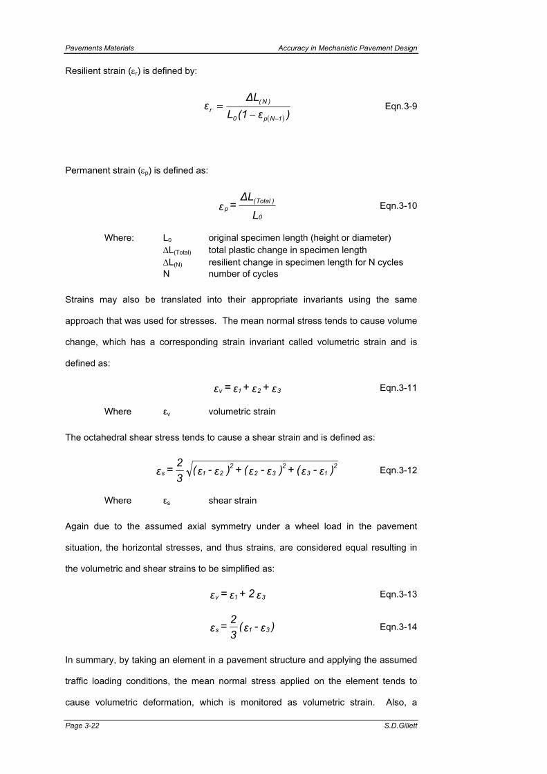
Pavements Materials Accuracy in Mechanistic Pavement Design
Page 3-22 S.D.Gillett
Resilient strain (εr) is defined by:
( ) )ε1(L
L∆ε
1Np0
)N(r
−−= Eqn.3-9
Permanent strain (εp) is defined as:
L
L∆ = ε
0
)Total(p Eqn.3-10
Where: L0 original specimen length (height or diameter) ∆L(Total) total plastic change in specimen length ∆L(N) resilient change in specimen length for N cycles N number of cycles
Strains may also be translated into their appropriate invariants using the same
approach that was used for stresses. The mean normal stress tends to cause volume
change, which has a corresponding strain invariant called volumetric strain and is
defined as:
ε+ε+ε= ε 321v Eqn.3-11
Where εv volumetric strain
The octahedral shear stress tends to cause a shear strain and is defined as:
)ε-ε(+)ε-ε(+)ε-ε(32 = ε 2
132
322
21s Eqn.3-12
Where εs shear strain
Again due to the assumed axial symmetry under a wheel load in the pavement
situation, the horizontal stresses, and thus strains, are considered equal resulting in
the volumetric and shear strains to be simplified as:
ε2+ε = ε 31v Eqn.3-13
)ε-ε(32 = ε 31s Eqn.3-14
In summary, by taking an element in a pavement structure and applying the assumed
traffic loading conditions, the mean normal stress applied on the element tends to
cause volumetric deformation, which is monitored as volumetric strain. Also, a

Accuracy in Mechanistic Pavement Design Pavements Materials
PhD Thesis Page 3-23
deviator stress applied to the element tends to cause shear deformation, which is
monitored by shear strain. However, there is also cross-coupling since shear stress
causes dilative or contractive volumetric stresses and due to the volumetric stress
change shear stresses are generated.
Stress Paths and p-q Diagrams
It is often desirable to depict the successive states of stress that exist in material as
the specimen is loaded and unloaded. The accepted method of showing this is to plot
a series of stress points {Boyce (1976)}.
These stress points have co-ordinates namely mean normal stress and deviator
stress and if these points are connected with a line or a curve. This curve is called a
stress path. By varying the stress path applied to the specimen a large number of the
stress regimes may be investigated. A sensible test approach is to load the specimen
along predetermined stress paths to simulate traffic loading on an element in a
pavement structure. A stress path, therefore, gives a continuous representation of
successive states of stress. For this work certain points are defined on a stress path,
such as the start and end points. These are illustrated in Figure 3-7. Note the
material failure line is also shown in this figure. This failure line is defined by
conducting strength tests in a standard triaxial apparatus.
Figure 3-7 The Definition of a Stress Path in p-q Space
Dev
iato
r Stre
ss (q
)
Failure Line for the Particular Material
stre
ss p
ath
(p , q )2 2
q = c x qmax failure
qfailure
Overburden Pressure (p )1
Mean Normal Stress (p)
(p , q )1 1

Pavements Materials Accuracy in Mechanistic Pavement Design
Page 3-24 S.D.Gillett
Possible Stress Path Regimes
During a repeated load triaxial test it is required that the vertical (σv) and horizontal
(σh) stresses applied to the specimen are greater than or equal to zero. Two stress
regimes can be applied to the specimen, namely:
• Compression, where σv > σh and q > 0, or;
• Extension, where σv < σh and q < 0.
With reference to Figure 3-8,
Taking the cell pressure (σc) to be zero for the compression stress regime:
σh = 0, σv > 0 and therefore ∆σv > 0, so
∆q = ∆σv and ∆p = ∆σv/3, therefore:
∆q/∆p = 3/1 shown as stress path (1).
Figure 3-8 Possible Stress Regimes in a Repeated Loads Triaxial Test
(1)
(3)
3 3
1 1
sc
-1
-3 -3
(4)
(2)
2
q
p
Impermissible areas as boundary stresses are negative,i.e. sv and/ or sh < 0.
Permissible areasi.e. sv and/ or sh ≥ 0.

Accuracy in Mechanistic Pavement Design Pavements Materials
PhD Thesis Page 3-25
Taking the cell pressure (σc) to be zero for the extension stress regime:
σh = 0, σv > 0 and therefore ∆σv > 0, as the cell pressure is increased
∆σc = ∆σh, which also increases ∆σv, therefore it is necessary to reduce ∆σv
by ∆σc so ∆σv = 0,
so ∆q = ∆σv - ∆σh = -∆σc, and ∆p = (∆σv + 2∆σh)/3 = 2∆σc/3, therefore:
∆q/∆p = -∆σc/(2∆σc/3) = -3/2 shown as stress path (2).
Taking the cell pressure (σc) greater than zero for the compression stress regime:
σh > 0, σv > σh > 0 and therefore ∆σv > 0, so
∆q = ∆σv - ∆σh = ∆σv and ∆p = (∆σv + 2∆σh)/3 = ∆σv/3, therefore
∆q/∆p = 3/1 shown as stress path (3).
Taking the cell pressure (σc) greater than zero for the extension stress regime:
σh > 0, σh > σv > 0 and therefore ∆σv < 0, so
∆q = ∆σv - ∆σh = -∆σv and ∆p = (-∆σv + 2∆σh)/3 = -∆σv/3, therefore
∆q/∆p = 3/1 shown as stress path (4).
3.4.5 Resilient Modulus and Poisson’s Ratio
In order to characterise unbound materials there are two important material
parameters, namely resilient modulus and Poisson’s ratio. Both of these parameters
are stress dependent, but assume linear elastic behaviour.
Hooke’s Law
These parameters are defined using Hooke’s Law. Hooke's law describes the linear
relationship between stress and strain for a uniaxial stress condition as shown in
Figure 3-9 and defined by:
z
z
εσE = Eqn.3-15
Where E Young’s modulus

Pavements Materials Accuracy in Mechanistic Pavement Design
Page 3-26 S.D.Gillett
Figure 3-9 Uniaxial Stress Condition Hooke’s Law
σZ
x εz
y z
Uni
t Len
gth
Unit Width
2εx
Hooke's law for the uniaxial case can be expanded to deal with a triaxial stress
condition where normal stresses act in x, y and z direction by superposing the strains
obtained from the above equations. The equations obtained are known as the
‘generalized Hooke's law’:
−−−−−−
=
3
2
1
3
2
1
σσσ
1ννν1ννν1
E1
εεε
Eqn.3-16
Where ε1; ε2; ε3 Normal strains σ1; σ2; σ3 Normal stresses
For the axisymmetric stress condition of the repeated load triaxial test, stresses and
strains in x and y direction are equal and these equations reduce and are the
equations that should be used to interpreted repeated load triaxial test results:
[ ]
( )[ ]313
311
σν1νσE1ε
νσ2σE1ε
−+−=
−=
Eqn.3-17
By replacing Mr for E the first of the equations in Equation 3-17 the equation can be
written as follows:
3
3r1
311r
σ2εMσ
ν
νσ2σεM
−=
−= Eqn.3-18

Accuracy in Mechanistic Pavement Design Pavements Materials
PhD Thesis Page 3-27
and then substituting this equation in the second of the equations in Equation 3-17:
( )
3
13r ε
νσσν1M −−= Eqn.3-19
133
1r13
33
1r13r σ
σε2εMσσ
σε2εMσσ2M
−−
+−= Eqn.3-20
33
13r2
113r312
3r σε2
εσMσεεMσσσ2M +−+−= Eqn.3-21
( )
33
2131
23
33
131r σε2
σσσσ2σε2
εσσ1M −−=
+− Eqn.3-22
( ) 13133
2131
23
r εσσσε2σσσσ2= M
+−−−
Eqn.3-23
Multiplying the top and bottom by -1 and including the subscript r for the repeated
triaxial case:
( )r3r1r3r1r1
2r3r3r1
2r1
r ε2εσεσσ2σσσ= M
−+−+
Eqn.3-24
Where ε1r; ε3r Repeated principal strains, ε1r=ε1(2)-ε1(1); ε3r= ε3(2)-ε3(1)
σ1r; σ3r Repeated principal stresses, σ1r=σ1(2)-σ1(1); σ3r=σ3(2)-σ3(1)
Then by substituting this equation into the second equation of Equation 3-18:
( )[ ] ( )
( )312
3131
12
3312
1313111
ε2εσ2εσσ2εσ2σσσε2εσεσσ = ν
−+−+−−+
Eqn.3-25
By dividing the top and bottom by -2σ3 and including the subscript r for the repeated
triaxial case the equation becomes:
( )r3r1r1r3r3
r1r3r3r1
σσεεσ2εσεσ = ν
+−−
Eqn.3-26
Equations 3-27 and 3-28, below, are then found from 3-24 and 3-26 respectively, by
substitution with Equations 3-5 and 3-7 for the case when u=0. If u≠0 then
Equation 3-17 and those following equations would need restating with σ’ in place of σ
and p’ in place of p.

Pavements Materials Accuracy in Mechanistic Pavement Design
Page 3-28 S.D.Gillett
These parameters can be defined in terms of p-q space and volumetric and shear
strain (by applying the equations defined above), again for the triaxial situation by:
vrrsrr
rrr εqεp9
qp9= M+
Eqn.3-27
vrrsrr
vrrsrr
εqεp9ε2qε3p5.4 = ν
+−
Eqn.3-28
Where: pr Repeated mean normal stress, (p2-p1) qr Repeated deviator stress, (q2-q1) εvr Change in volumetric strain, (εv2-εv1) εsr Change in shear strain, (εs2-εs1)
3.5 SUMMARY
Pavement materials exhibit two distinct types of behaviour when placed under the
traffic loads:
• Elastic behaviour, which determines the load spreading ability of the layer, which
manifests as cracking due to fatigue of the upper layers, and;
• Permanent deformation, which causes a build up of irrecoverable deformation,
which after a number of load applications becomes apparent as rutting.
The structural capacity of a road pavement is often determined by the most critical
structural behaviour (as above) in one of the layers that make up the pavement.
Although analytical mechanistic pavement design procedures are recognised as being
superior to the traditional empirical methods there are some difficulties in establishing
the parameters required for this type of design. Analytical mechanistic design
requires fundamental material properties such as values for resilient modulus and
Poisson’s ratio. Work correlating empirical and analytical methods have shown
considerable errors resulting in the conclusion that a direct test method of measuring
the material properties accurately is required – repeated load triaxial is one such
method. In general the stresses experienced by an element of soil or aggregate in a
pavement structure under traffic loading can be simulated in the laboratory on
representative samples using the repeated load triaxial apparatus.

Accuracy in Mechanistic Pavement Design Pavements Materials
PhD Thesis Page 3-29
The principle of repeated load triaxial tests is to simulate an element in a pavement by
manufacturing a specimen of road construction material and applying similar load
conditions to those that might be experienced in the field while measuring the
deformation experienced by the specimen.
The purpose of the repeated load triaxial test is to determine the elastic parameters of
materials, namely the resilient strain parameters and permanent strain parameters.
Due to the stress dependent behaviour of these materials the elastic parameters must
be determined at a number of stress levels.
Road construction specifications require all materials to be tested for suitability. In
order to use road construction materials optimally a better understanding of the
properties of these materials under traffic loading is necessary. This may be possible
using sophisticated test apparatus to characterise the materials under simulated traffic
loading, however, these sophisticated tests are often prohibitively expensive.
The loading applied to a specimen under repeated load triaxial testing is simplified by
ignoring the rotational stresses applied when a load passes over a element. This
limitation is made up for in the relative simplicity of the repeated triaxial apparatus in
comparison to other test methods however. Thus this work only considers repeated
load triaxial testing of materials in order to understand the behaviour of materials in a
laboratory.
There are basically three different repeated load triaxial apparatus configurations as
follows:
• Conventional repeated load triaxial test, with constant confining pressure;
• Internal vacuum repeated load triaxial test, with constant confining pressure;
• Variable confining pressure repeated load triaxial test.

Pavements Materials Accuracy in Mechanistic Pavement Design
Page 3-30 S.D.Gillett
Possible errors in testing material due to apparatus produced factors are as follows:
• Specimen Alignment
• Seating Errors and Bedding Errors
• End Friction or Restraint
• System Compliance
• Deformation Measurement
It is often desirable to depict the successive states of stress that exist in material as
the specimen is loaded and unloaded. These stress points have co-ordinates namely
mean normal stress and deviator stress and if these points are connected with a line
or a curve called a stress path.
Stress paths, plotted in p-q space, allow different stress regimes to be applied to a test
specimen in a repeated load triaxial apparatus. Theoretically it is possible to apply
both comprehensive and tensile stresses to a specimen however unbound materials
will only allow small tensile stresses due to pore water suctions and inter-granular
friction.
Since unbound granular materials are used in layers nearer the surface of the
pavement structure it may be argued that it is more important to correctly categorise
these materials, rather than subgrade soils, since they are more heavily stressed.
In order to characterise unbound materials there are two important material
parameters, namely resilient modulus and Poisson's ratio. Both are ratios describing
the strain response to stress. Although often treated as properties of a material, it will
be shown in Chapter 5 that strain has a non-linear relationship with applied stress for
typical pavement foundation materials, thus these parameters are non-constant, and
depend on the stress level for their magnitude.

Accuracy in Mechanistic Pavement Design Material Behaviour
PhD Thesis Page 4-1
4 FACTORS THAT INFLUENCE THE BEHAVIOUR OF MATERIALS IN PAVEMENTS
4.1 INTRODUCTION
Much effort has been devoted to characterising the resilient behaviour of road
construction materials. To accommodate the non-linearity of these materials the
resilient response is usually defined by resilient modulus and Poisson's ratio or
alternatively, the use of shear and bulk moduli has been suggested. This will be
discussed in the forthcoming chapters.
Rut development is a common mode of failure in flexible road pavements. The
prediction of the permanent deformation development within a pavement structure is
extremely complex, and it is probably due to this that, in comparison to resilient
behaviour, less research has been devoted to the permanent deformation
development in road construction materials.
For the design of pavements using road construction materials it is important to
consider how the resilient and permanent behaviour varies with changes in other
influencing factors as discussed below.
Although stress has a major effect on granular material behaviour, there are other
characteristics that are likely to affect the behaviour of granular material under
loading.
4.2 ENVIRONMENTAL CONDITIONS (MOISTURE IN PAVEMENTS)
The structural design of road pavements is usually based on material properties in the
soaked condition (highly saturated). It is possible to examine the effect of various
moisture conditions on pavement performance, particularly equilibrium conditions and
seasonal fluctuations, provided the appropriate material properties can be measured.
It is not usually realistic, however, to design pavements on the equilibrium condition,
because temporarily abnormally wet conditions may have an overriding effect due to
the greatly weakened properties of the pavement material layers at that time.
Where roads are constructed on clayey subgrades, unbound granular subbases are
often placed directly on the subgrade or in the case of weak foundations on a low

Material Behaviour Accuracy in Mechanistic Pavement Design
Page 4-2 S.D.Gillett
quality capping layer comprising local material that may contain some plastic fines.
This construction practice can lead to water travelling upward through the high
capillary rise subgrade into capping layer and subbase. The general principles of the
interaction between unbound materials and water in the foundation and upper
granular layers will be discussed here.
The foundation must perform in the longer term as a support system to the completed
pavement. The stress levels applied will be much lower since the traffic loading will
largely be supported by the pavement structure and the expected future moisture
condition should have been anticipated during the pavement structure design. It is
probable that, some time after construction, the equilibrium water condition will be
reached. If this is higher than the moisture content during construction, failure could
occur due to weakening of the foundation. The wetting of unbound granular base and
subbase layers can cause a substantial reduction in material strength and stiffness,
depending on the composition of the material.
4.2.1 Principles of Unbound Material and Water Interaction
Soils and granular materials may be defined as an assemblage of discrete particles
with variable amounts of water and air among the particles. Solid particles are in
contact with one another forming the soil skeleton and the spaces between them form
a system of interconnecting voids or pores.
There are three states in which these materials may exist with respect to water and air
content:
i) Dry Voids contain only air
ii) Saturated Voids are full of water
iii) Partially saturated Voids contain both water and air
This is shown schematically in Figure 4-1.

Accuracy in Mechanistic Pavement Design Material Behaviour
PhD Thesis Page 4-3
Figure 4-1 Pore Pressure in Pavements
SurfaceDry
Saturated
Water TablePore Pressure (-ve) Pore Pressure (+ve)
Saturated
Partially saturated. Water between particles not connected
Partially saturated. Water between particles connected
When loaded the compressive forces are considered to be positive. It is easy to
envisage that, in a dry soil, the compressive forces are transmitted between particles
at their points of contact. Therefore, the stiffness is directly related to the density of
the material.
In the case of saturated materials, all of the voids in the material are filled with water.
This may occur during periods of severe flooding and it can have severe
consequences. Since the material and the water are virtually incompressible the
application of a compressive stress will lead to a substantial build up of pore water
pressure particularly in poorly drained conditions. Saturated granular materials also
develop excess pore-water pressure under repeated loading. As pore-water pressure
develops the effective stress in the material decreases with a subsequent decrease in
both strength and stiffness of the material. Therefore, considering positive pore water

Material Behaviour Accuracy in Mechanistic Pavement Design
Page 4-4 S.D.Gillett
pressure occurring in a fully saturated soil, then the effective stress as defined by
Terzaghi (1943) states that:
uσ = σ −′ Eqn.4-1
Where: σ' Effective stress σ Total stress u Pore water pressure
This principle was developed for saturated conditions and is therefore only valid in
case of positive pore water pressures (u > 0). In case of partial saturation, negative
pore water pressures (u < 0) occur and this law cannot be used directly.
The partially saturated condition in soils and unbound granular materials is far less
simple. Under these conditions, which are the norm for roads, capillary forces retain
the water in the unbound material layer against the gravitational forces that endeavour
to drain the water out of the material and against evaporation of the water through the
surface or side slopes. These capillary forces are caused by the curved air-water
interfaces in the voids of the material. The tensile stress with which water is held in
the material is termed the suction and since it increases the effective stress in
Equation 4-1 it is a positive quantity.
However, if the water is connected in a continuous column and no upward flow is
assumed, although in reality due to evaporations upward flow is expected, then the
pore water pressure is hydrostatic. If the water particles in the soil matrix are
discontinuous then the suction in each of the particles of water will take on the tension
as established by the surface tension. In certain cases this may result in huge values,
although the overall effect on effective stress will be less marked as the suction only
acts at those points where particles of water exist and not uniformly across the whole
soil. Therefore based on the complexity of the partially saturated conductions this part
of the curve may vary from high to low tension as shown in Figure 4-1 by the hatched
region.

Accuracy in Mechanistic Pavement Design Material Behaviour
PhD Thesis Page 4-5
4.2.2 Suction
Croney (1977) stated that water is held in the soil matrix by absorption and surface
tension forces at a pressure less than atmospheric, which he called soil moisture
suction, or suction. He defined suction as a measure of the pressure required to
abstract water from a sample of soil, which is free from external loading. Suction is
expressed on the pF scale, which is the common logarithm of the height in
centimetres of an equivalent column of water.
Different materials types have different soil-suction characteristics. Coarse granular
materials have small surface forces because of the low surface areas and the nature
of the surfaces and, therefore, capillary forces dominate. Consequently, the suction
potential is zero when these materials are saturated and completely dry. In both
cases, no curved air-water interfaces exist and, therefore, no capillary forces are
present. The maximum suction potential is reached somewhere in the unsaturated
region of partly filled pores.
Clay particles have a far larger surface area per unit weight than larger granular
particles. Furthermore, the surface of clay particles has an electric charge. Due to
these electric charges the surface forces of clays may dominate over the capillary
forces and can cause very large suction potentials in quite dry clays.
It is the effective stress that dominates aspects of soil behaviour such as compression
and strength. Since both the total stress and the pore water pressure can be
measured or calculated, depending on the situation in the laboratory or the field, the
effective stress can easily be calculated. It is for this reason that most triaxial testing
of clays is still being done under fully saturated conditions, thereby allowing
Equation 4.1 to be used. Sands can be tested either in the fully saturated condition or
completely dry. In the latter case, the whole problem of pore water pressures (positive
or negative) simply does not occur. It was noted by Barksdale et al (1990) that the
determination of unsaturated soil strength is particularly problematic since the
accurate determination of the pore air pressure within the material is very difficult
indeed.

Material Behaviour Accuracy in Mechanistic Pavement Design
Page 4-6 S.D.Gillett
4.2.3 Material Stiffness Related to Water Content
In addition to its effect on soil strength, suction also has a significant effect on the
stiffness of soils. Since this stiffness plays an important role in pavement design and
analysis, the influence of suction should be taken into account.
As stated above the standard approach used in pavement design, for the
determination of stiffness parameters of unsaturated soil is to test the specimens that
are prepared at the worst possible field moisture content and analysing the test results
in terms of total stresses. Thompson and Robnett (1979), for instance, tested
unsaturated subgrade soils for resilient characteristics using a repeated load triaxial
apparatus. The specimens were prepared at and above the optimum moisture
content and the resilient modulus was calculated as the ratio of the applied deviator
stress to the recoverable axial strain of the triaxial specimen. The degree of
saturation of the soils was shown to have a considerable effect on the resilient
modulus, but no attempt was made to relate the resilient modulus to suction.
The degree of saturation of most untreated granular materials has been found to
affect the elastic stiffness of road construction materials in both laboratory and in situ
conditions. It is generally agreed that the resilient characteristics of dry and partially
saturated granular materials is similar, but as complete saturation is approached the
resilient behaviour may be affected significantly {Haynes and Yoder (1963), Hicks and
Monismith (1971), Smith and Nair (1973); Barksdale and Itani (1989), Dawson et al
(1996); Vuong (1992); Heydinger et al (1996)}
In resiliency testing of soils at high degrees of saturation, care should be taken when
dealing with low permeability soils. Volume change can readily turn the negative pore
water pressure (suction) in the triaxial specimen into a positive pore water pressure,
since the low permeability prevents sufficient drainage. This may lead to a drastic
reduction of the resilient modulus or even to specimen failure. In granular materials
with a high permeability, these problems of positive pore water pressures do not occur
provided the triaxial specimen is allowed to drain freely. Because of the relatively low
value of suction in these materials, test results can be interpreted in terms of total
stresses in the case of testing for practical purposes.

Accuracy in Mechanistic Pavement Design Material Behaviour
PhD Thesis Page 4-7
For research purposes, test results should be interpreted in terms of effective
stresses. Providing that the material does not contain a significant amount of clay,
this can be performed by testing the material in the completely dry condition. As
suction will be caused by capillary effects, when completely dry this will be equal to
zero. Effective stresses are then equal to total stresses and test results can be
interpreted correctly without the need for measurement of suction.
For subgrade soils that contain significant amounts of clay, the simple approach of
testing in the completely dry condition cannot be used. The clay causes a large
suction in the material, which is at a maximum in the dry condition, and can therefore
not be ignored. The resilient modulus of saturated clayey materials is usually
expressed as a function of two stress variables, namely the confining stress and the
deviator stress. Fredlund et al (1975) stated that, in case of unsaturated soils, a third
stress variable (the suction) should be added.
Later, from experiments, Fredlund et al (1977) showed that the influence of the
confining stress was negligible compared to the effect of the deviator stress and the
suction and suggested the following equation:
qmcMlog d1d1r −= Eqn.4-2
Where c1d and m1d are functions of soil suction
It must be noted that expressing the resilient modulus as a function of these three
stress variables requires the measurement of the pore air pressure and pore water
pressure during the repeated load triaxial test and Fredlund et al (1977) reported
serious technical problems with this measurement.
It is also reported that the preparation of triaxial specimens at a specific suction level
is cumbersome. It took Paute et al (1986) a minimum of one month per specimen to
reach a specified suction level. The triaxial specimen was placed between two high
air-entry porous discs, which were connected to a water vessel placed at a preset
level below the triaxial specimen, thereby obtaining the required negative pore water
pressure. By connecting a geotextile, which was placed between the triaxial

Material Behaviour Accuracy in Mechanistic Pavement Design
Page 4-8 S.D.Gillett
specimen and the membrane down the side of the specimen, to the atmosphere, the
pore air pressure was kept at atmospheric pressure.
An analysis of the results presented by Brown et al (1975) in terms of suction show a
linear relationship between resilient modulus and suction at constant deviator stress.
A similar relationship is reported by Finn et al (1972) determined with data from tests
on a road subgrade. Dehlen (1969), working with silty clay, showed a measured
suction decreasing with increasing depth below a road surface and a corresponding
linear decrease in resilient modulus with suction. Croney (1977) states that soil
moisture suction is an overriding factor in determining the elastic modulus for
saturated clays. Fredlund et al (1975) measured the resilient modulus and suction of
a till and a clay and found that the modulus increased with increasing suction, but at a
decreasing rate.
In pavements the total time actually under load is small {Knight and Blight (1965)} and
it is therefore reasonable to assume that there is some drainage although individual
load pulses themselves are undrained. France and Sangrey (1977) allowed some
continuous drainage during their cyclic tests, but not sufficient to inhibit the build up of
pore pressures. Brown et al (1977), Anderson et al (1976), and Overy (1982) have all
considered this problem. The general conclusion is that samples on the wet side of
critical, with positive excess pore pressures, expel water and become stiffer while
those on the dry side, with negative residual pore pressures will tend to imbibe water
and soften
It was argued by Lekarp et al (2000a) that it is not the degree of saturation that
influences the material behaviour but rather that the pore pressure response controls
deformational behaviour. Mitry (1964), Seed et al (1967), and Hicks (1970) and
Pappin (1979) all reported that if the test results are analysed on the basis of effective
stresses, the resilient modulus remains approximately unchanged at any particular
effective stress.

Accuracy in Mechanistic Pavement Design Material Behaviour
PhD Thesis Page 4-9
Saturation of unbound granular materials also affects the resilient Poisson's ratio.
Hicks (1970) and Hicks and Monismith (1971) reported that Poisson's ratio is reduced
as the degree of saturation increases.
As stated above excessive pore pressure reduces the effective stress, resulting in
diminishing permanent deformation resistance of the material {Haynes and Yoder
(1963); Barksdale (1972a); Maree (1982); Thom and Brown (1987); Dawson et al
(1996)}. The stress-strain behaviour of soils and granular materials can be improved
significantly by draining the system {Lekarp et al (2000a)}.
4.3 COMPACTION (DENSITY) OF PAVEMENT LAYERS
During road construction, engineers strive for high material compaction, which
increases the density of the material, and is well known to alter its response to static
loading, causing it to become both stiffer and stronger. Heavy compaction equipment
is used to densify relatively thin layers of subgrade, subbase, base, and surfacing.
After constructing a particular layer, this layer becomes a temporary working surface
for the next layer and so on. Usually these compaction stresses are the greatest
stresses to which a particular layer is ever subjected.
The application of large vertical stresses during construction is reported to cause
lateral stresses to develop that become locked into both granular bases and cohesive
subgrades {Sowers, et al., (1957); Uzan, (1985); Selig, (1987); Duncan and Seed,
(1986)}. Thom and Brown (1988) and Brown and Selig (1987) stated that the effect of
density on resilient modulus is relatively insignificant but that density appeared to have
some influence on Poisson's ratio {Barksdale and Itani (1989)}.
It is surmised that the reason that density does not have a great effect on resilient
modulus is because when a load is applied to a pavement material the particles move
relative to one another changing the stress between them accordingly (σ’ and u). As
the load is removed they return to their original positions and thus this is independent
of density, density may, however, effect the distance moved. Poisson’s ratio is
affected by the variation in density and this thought to be because a more dense
Material Behaviour Accuracy in Mechanistic Pavement Design
Page 4-10 S.D.Gillett
material is more likely to transmit movement through particles, therefore vertical load
will cause more horizontal movement for a more dense material.
The effect of density, as described by degree of compaction, has been regarded in
previous studies as being significantly important for the long-term behaviour of
granular materials {Holubec (1969); Barksdale (1972b), Barksdale (1991); Allen
(1973); Marek (1977); Thom and Brown (1988)}. Resistance to permanent
deformation in these materials under repetitive loading appears to be highly improved
as a result of increased density.
4.3.1 Compaction of Granular Bases
It was shown by Selig (1987) that in a granular layer, large plastic lateral strain
develops in the bottom of the layer during the first cycle of loading. Upon subsequent
loading cycles, however, the response rapidly approaches an elastic condition. The
lateral stress in the bottom of the granular layer, in both the loaded and unloaded
condition, gradually increases up to about 50 load cycles. After 50 load cycles the
lateral stresses in both the loaded and unloaded states were found to be in the order
of 20 times greater than before the first load cycle. The horizontal stress in the
unloaded condition, however, was larger than the stress existing when fully loaded
which was not true when loading first started. These important findings indicate that
the stress increment in the bottom of the granular base caused by loading becomes
tensile after a relatively few load cycles. However, when added to the existing
residual lateral stress, a net compressive state of stress exists in the bottom of the
granular layer. It was concluded by Selig (1987) that the residual lateral stress is the
most important factor limiting permanent deformation of the bottom of the granular
base and therefore is also an important factor in determining the appropriate stress
state at which to evaluate the resilient modulus. The residual lateral stress is
relatively large and can be expressed by:
00hr σKσ = Eqn.4-3
Where: σhr Residual lateral stress σ0 Vertical overburden stress Ko Coefficient of lateral earth pressure

Accuracy in Mechanistic Pavement Design Material Behaviour
PhD Thesis Page 4-11
The coefficient of lateral earth pressure for this condition is greater than unity but less
than the passive coefficient of earth pressure that represents a limiting condition of
failure due to lateral movement outward. For a granular material the passive
coefficient of earth pressure is equal to:
+=
2θ45tanK 2
p Eqn.4-4
Where: ϕ Angle of internal friction for the granular material
The work of both Selig (1987) and Uzan (1985) indicate the great importance in
properly considering the residual stress that exists in a granular base in the analyses
used in mechanistic based pavement design procedures.
4.3.2 Compaction of Cohesive Subgrade
Uzan (1985) stated that residual lateral pressures were observed for both
cohesionless and cohesive soils. Uzan (1985) and Duncan and Seed (1986)
proposed methods of analysis for predicting residual lateral stresses due to
compaction of cohesive soils. Sowers, et al (1957) investigated the residual lateral
stresses produced by compacting soil in a steel mould. This study indicated that the
residual stresses became less with increasing moisture content, and decrease sharply
at moisture contents close to the optimum value. Also, Sowers, et al (1957) reported
that, for the clay tested, the residual stresses induced by static compaction were
higher than those induced by impact compaction. Relatively high values of residual
stresses were measured due to compaction of soils in a confined cylinder, which does
not duplicate the free field conditions existing during fill placement.
4.4 THE EFFECT OF STRESS LEVELS
The literature shows that stress level has a significant impact on resilient properties of
road construction materials. However deviator stress has been found to be much less
influential on material stiffness than confining pressure and the sum of principal
stresses {Mitry (1964), Monismith et al (1967), Hicks (1970), Smith and Nair (1973),
Uzan (1985), and Sweere (1990)}. Monismith et al (1967) reported an increase as
great as 500% in resilient modulus for a change in confining pressure from 20 to

Material Behaviour Accuracy in Mechanistic Pavement Design
Page 4-12 S.D.Gillett
200 kPa and Smith and Nair (1973) observed that an increase of about 50% in
resilient modulus was observed when the sum of principal stresses increased from 70
to 140 kPa.
Hicks (1970), Brown and Hyde (1975), and Kolisoja (1997) have all reported that
Poisson's ratio of unbound granular materials increases with increasing deviator
stress and decreasing confining pressure, implying that the resilient Poisson's ratio is
also influenced by the state of applied stresses.
It is well known {Lashine et al (1971) and Brown and Hyde (1975)} that there is a
threshold value of repeated deviator stress magnitude, above which the sample
eventually fails and below which an equilibrium state is reached regardless of the
number of further cycles. Lashine et al (1971) reported that during triaxial testing the
measured permanent axial strain settled down to a constant value that is directly
related to the ratio of deviator stress to confining pressure.
4.5 LOAD DURATION AND FREQUENCY
Boyce et al (1976) showed that the limestone material they tested in a triaxial
apparatus was subjected to stress history effects. They stated that pre-loading with a
few cycles of the current loading regime and avoiding high stress ratios in tests for
resilient response could reduce these. Brown and Hyde (1975) and Mayhew (1983)
reported that resilient characteristics of unbound granular materials are basically
insensitive to stress history, provided the applied stresses are kept low enough to
prevent substantial permanent deformation in the material. Therefore, large numbers
of resilient tests can be carried out sequentially on the same specimen, to determine
the resilient parameters of the material.
The general view regarding the impact of load duration and frequency on the resilient
behaviour of granular materials is that these parameters are of little or no significance
{Seed et al (1967), Morgan (1966), Hicks (1970), Boyce et al (1976), and Thom and
Brown (1987)}
Permanent strain continuously increases under repeated loading {Morgan (1966);
Barksdale (1972); Sweere (1990)}. Morgan (1966), for instance, applied up to

Accuracy in Mechanistic Pavement Design Material Behaviour
PhD Thesis Page 4-13
2,000,000 load cycles and reported that permanent strain was still increasing at the
end of the tests. Barksdale (1972) concluded that permanent axial strain in untreated
granular materials accumulates linearly with the logarithm of the number of load
cycles. However, Brown and Hyde (1975) noted that an equilibrium state was
established after approximately 1,000 load applications. Paute et al (1986) stated that
the rate of increase of permanent strain in granular materials, under repeated loading,
decreases constantly to such an extent that it is possible to define a limit value for the
accumulation of permanent strain.
4.6 LOADING HISTORY
Brown and Hyde (1975) showed that resilient characteristics of unbound granular
materials are not affected by loading history. They showed that a large number of
stress paths can be applied to a specimen for the determination of resilient
parameters, provided that the stresses applied are kept well below the failure line for
the material.
Brown and Hyde (1975) reported that permanent strains in unbound granular
materials are, on the contrary, affected significantly by loading history. Therefore,
several triaxial specimens have to be tested to obtain the relationship between stress
ratio applied and permanent deformation. Each test usually involves a large number
of load applications on each specimen, which renders the determination of permanent
strain characteristics to be quite time consuming. This is probably the reason why far
less data is available on permanent deformation of unbound granular materials than
there is on resilient deformation.
Kalcheff and Hicks (1973) investigated the effects of load duration and load frequency
on the resilient modulus and showed no quantifiable effect of load duration on the
resilient modulus.
4.7 THE EFFECT OF MATERIAL PROPERTIES
Thom and Brown (1988), Brown and Selig (1991) and Raad et al (1992) all concluded
that the stiffness of road construction material is, in some degree, dependent on
particle size and its distribution.

Material Behaviour Accuracy in Mechanistic Pavement Design
Page 4-14 S.D.Gillett
Selig and Roner (1987) stated that flaky particles, at stresses which do not lie along
the failure line, increase the shear strength of granular material, however, the
disadvantage being that an increase in the flakiness may cause problems of
breakage, abrasion, increased permanent strain and decreasing stiffness of the
material.
Aggregate type may have a significant effect on the resilient modulus when other
parameters such as grading, density and applied stress are kept constant. Barksdale
and Itani (1989) tested different granular materials with the same grading and they
found that angular materials had a higher resilient modulus than rounded gravel, the
increase being about 50% at low mean normal stress conditions decreasing to about
25% at high mean normal stress levels.
Thom (1988) and Thom and Brown (1989) carried out repeated load triaxial tests on
different granular materials, and concluded that the resilient modulus of granular
materials at low strain levels may be influenced by particle texture, that a correlation
exists between elastic stiffness and the surface friction properties of materials, and
that high resilient modulus and good load spreading properties in the pavement may
be expected from material with angular to sub-angular shaped particles and a very
rough surface when compared with material with sub-rounded or rounded particles
and a smooth surface.
4.8 SUMMARY
The basic principles of road design, the dependence on traffic loading prediction and
assessment of the subgrade strength have remained unchanged for centuries.
Naturally, it is fundamental that the properties and characteristics of the construction
materials are known and understood.
Not only are the properties of the materials themselves important but it is also
important that an understanding of the way that different material layers in a pavement
mechanism interact. For example cracking of an asphalt surface layer is probably a
consequence of weaknesses in the granular base. Pavement behaviour can also be

Accuracy in Mechanistic Pavement Design Material Behaviour
PhD Thesis Page 4-15
influenced by other imposed conditions such as environmental conditions, moisture,
loading magnitude, duration and frequency, for example.
For the design of pavements using road construction materials it is important to
consider how the resilient and permanent behaviour varies with changes in other
influencing factors. A number of factors are likely to influence the behaviour of
unbound materials in pavements, namely:
• Environmental conditions (moisture in pavements), particularly suction which has
a significant effect on the stiffness of soils.
• Compaction (density) of pavement layers.
• The effect of stress levels.
• Load duration and frequency.
• Loading history.
• The effect of material properties.
It is concluded that the preparation of triaxial specimens at specified suction levels
requires sophisticated equipment and, more importantly, a great deal of time. A more
practical approach is the preparation of triaxial specimens at field moisture content
and measuring the suction in the specimen using some device.
All road construction materials, unbound granular materials and subgrade soils, are
heavily stress dependent.


Accuracy in Mechanistic Pavement Design Analytical Models
PhD Thesis Page 5-1
5 ANALYSIS OF THE BEHAVIOUR OF THE MATERIALS BY MODELLING
5.1 INTRODUCTION
The main objective in testing the materials in the laboratory is to determine the
material parameters, such as the resilient modulus, from the test results. These
parameters can be used to define the suitability or otherwise of the material in road
construction. This may apply to foundation materials that will inevitably form part of
the pavement structure or imported borrow materials to be used to construct the upper
structural layers. A number of constitutive relationships have been developed and are
presented here. These relationships require that model coefficients are determined
for each of the materials tested during the ‘Science Project’. By incorporating the
parameters obtained from the relationships into mechanistic pavement design the
most economic use of available materials in terms of layer thickness and structural life
can be determined. It is important that accurate coefficients for the relationships are
obtained and the magnitude of any errors appreciated by practising engineers.
During this work (as will be presented) recorded values, stresses and strains, are
obtained from repeated load triaxial testing. This chapter describes how these results
may be analysed using constitutive relationships in which model coefficients and
subsequent material parameters can be determined. The aim of these models is to
predict the behaviour of the materials under traffic loading.
5.2 MODELLING THE EXPERIMENTAL DATA
To analyse different pavement structures, constructed using different materials,
certain material characteristics must be determined. These vary from simple values
determined from simple laboratory testing, for example failure characteristics yielding
relationships between resilient modulus and CBR, to more complex characteristics
which, in practice, are often estimated from simple material characteristics rather than
the results of complex of testing.
In order to examine the effect of using different constitutive relationships for the
analysis of road construction materials a range of different relationships have been

Analytical Models Accuracy in Mechanistic Pavement Design
Page 5-2 S.D.Gillett
considered. These relationships vary from relatively simple models (k-theta model) to
more complex models (Mayhew model) described later. Some of the more simple
models are used in practice, for example in the AASHTO (1993b) and Austroads
(1992) procedures. With the advent of more powerful personal computer based
analytical computer methods, such as finite element analysis, more complex models
will become more common in pavement design. Of course, it does not necessarily
follow that the greater the complexity of the relationship the better the accuracy of the
predictions made by the model. Naturally these relationships require accurate input
data, since if estimations of complex material characteristics are made from
inappropriate material tests then the models will make erroneous predictions.
During the analysis of an artificial specimen in the forthcoming chapter it will be shown
that some consideration of the applied stress is necessary in order to compare results
from different sources since the applied stresses are not always identical. The
computation of bulk and shear modulus for this artificial material was calculated and
from these values the resilient modulus and Poisson’s ratio were determined allowing
comparisons to be made. During the repeated load triaxial laboratory tests on
materials strains are measured under predetermined stress conditions and since
these materials are heavily stress dependent it is important that both stresses and
strains are considered during modelling.
Suppose that the observed strain response to a cyclic application of a deviator stress
is represented by the black path in Figure 5-1, ACBA (which would be a typical
response). Then this is normally modelled in one of three ways, namely:
• Linear elastic behaviour
The stress strain curve is assumed to be a straight line connecting
A to B under loading and to return along the identical path (B to A)
when unloaded (Figure 5-1a). Thus a single value for resilient
modulus can be found, namely the slope of the vector, irrespective
of the magnitude of B, even if the actual stress applied (and
resulting strain) is indicated by (for example) point C.

Accuracy in Mechanistic Pavement Design Analytical Models
PhD Thesis Page 5-3
• Non-linear elastic behaviour
The stress strain curve is assumed to be the lines that connects A
to C, D and B. This curve is assumed to apply under both loading
and unloading. It is common to describe this behaviour by the
equivalent linear modulus which would represent the same
maximum stress-strain. Thus the resilient modulus varies with the
magnitude of maximum stress applied, and may be defined by the
slope of the vector which connects the relevant point (e.g. the lines
A-C, A-D or A-B in Figure 5-1b).
• Non-linear inelastic behaviour
The stress strain curve follows the exact path as shown by the
black line in Figure 5-1c for both the loading element and the
unloading element of the curve. If this behaviour is to be described
by an equivalent linear modulus (because only the end points are
of interest) then it is modelled no differently from the preceding
case. However, if the strain path is to be computed then some
other model will be required - for example a tangent resilient
modulus which varies with the magnitude of stress and varies for
the loading and unloading cases.
Figure 5-1 Definition of Linearity and Elasticity
Stress B Stress B Stress B
D
C C
A A A
Strain Strain Strain
a. b. c.Linear Elastic Behaviour Non-Linear Elastic Behaviour
Non-Linear Inelastic Behaviour
Note: the black loop it taken to be the actually path as the material is loaded and unloaded.

Analytical Models Accuracy in Mechanistic Pavement Design
Page 5-4 S.D.Gillett
The non-linearity of these characteristics of a road construction material is illustrated
in Figure 5-2, this figure shows the resilient modulus and Poisson’s ratio as a function
of the deviator stress applied on a triaxial specimen. The resilient modulus is clearly
dependent on the deviator stress, whereas the Poisson's ratio proves to be more
constant for this example for the specimen of London Clay. For the sample of Soft
Limestone shown in Figure 5-3 the reverse can be seen, the Poison’s ratio is
dependent on the deviator stress, whereas the resilient modulus appears more
constant.
Figure 5-2 Stress Dependency of the Resilient Modulus and Poisson’s Ratio for a Sample of London Clay
0
10,000
20,000
30,000
40,000
50,000
60,000
70,000
80,000
0 10 20 30 40 50 60 70 80Deviator Stress (qr) [kPa]
Res
ilient
Mod
ulus
(Mr)
[kPa
]
LNEC UNOT LRCF
0.0
0.2
0.4
0.6
0.8
1.0
1.2
0 10 20 30 40 50 60 70 80Deviator Stress (qr) [kPa]
Pois
son'
s ra
tio [ ν
]

Accuracy in Mechanistic Pavement Design Analytical Models
PhD Thesis Page 5-5
Figure 5-3 Stress Dependency of the Resilient Modulus and Poisson’s Ratio for a Sample of Soft Limestone
0
200,000
400,000
600,000
800,000
1,000,000
1,200,000
1,400,000
0 20 40 60 80 100 120 140 160 180 200Deviator Stress (qr) [kPa]
Res
ilien
t Mod
ulus
(Mr)
[kPa
]
0.0
0.1
0.2
0.3
0.4
0.5
0.6
0.7
0.8
0.9
1.0
0 50 100 150 200Deviator Stress (qr) [kPa]
Poi
sson
's ra
tio [ ν
]
Empirical pavement design methods require the resilient modulus and Poisson’s ratio
to be constant {Ahlborn (1963)}, therefore, it is desirable to define the most relevant
resilient modulus and Poisson’s ratio for each material specimen tested. Since these
parameters are stress dependent, they should be defined at the characteristic stress
level pertinent to the material in the pavement. In Chapter 2 the characteristic stress
levels, in terms of deviator and mean normal stresses, were defined for an unbound
granular material and a subgrade soil.

Analytical Models Accuracy in Mechanistic Pavement Design
Page 5-6 S.D.Gillett
5.3 CONSTITUTIVE RELATIONSHIPS TO DEFINE THE BEHAVIOUR OF MATERIALS
The models and corresponding parameters that are to be used for the analysis can be
divided into three categories, namely those:
• For all road construction materials;
• For subgrade soils, and;
• For unbound granular materials.
In order to allow the dimensions of the coefficients used by these models to be non-
dimensional a constant pa has been introduced, pa is taken to be atmospheric
pressure. This non-dimensionality is not generally the case in the original forms of the
models.
5.3.1 Models for all Road Construction Materials
Simple Linear Elastic Model
The simple linear elastic model simply defines a characteristic resilient modulus and
Poisson’s ratio. These parameters are calculated from the experimental data for each
stress path. They are calculated using the equations in Chapter 3 and are thus stress
dependent since they depend on the stress applied to the specimen.
Constantν
Constant = M
c
r
= Eqn.5-1
Where Mr Characteristic resilient modulus, MPa νc Characteristic Poisson’s ratio, constant

Accuracy in Mechanistic Pavement Design Analytical Models
PhD Thesis Page 5-7
The k-theta model
The k-theta model {Hicks and Monismith (1971)} is an early model and in quite
common use. It is a simple model for the resilient modulus that has 2 model
coefficients (k1 and k2) and two material parameters (Mr and ν).
( )
Constantν
θ k = Morp
3p k = M
c
k1r
k
a
21r
2
2
=
Eqn.5-2
Where: p2 Maximum mean normal stress, (3p2 = theta), kPa pa Atmospheric pressure, pa = 100 kPa k1, k2 Model coefficients
The k-theta model has been used for design of new pavements {Thompson (1992)} or
pavement evaluation {Brown and Almeida (1993)}. However, it has some drawbacks,
the Poisson’s ratio is not modelled and a constant characteristic value for this
parameter needs to be defined. Although experimental values show that Poisson’s
ratio is not constant, for this work, the Poisson’s ratio is defined by the value
determined at the characteristic stresses mentioned above. Secondly, this model
does not allow directly for any change in the deviator stress applied, which means it is
best used for low shear levels which is not generally the case for pavements,
particularly the upper layers {Uzan (1985)}. Thirdly the model has been developed
from simple laboratory triaxial test results in which the initial deviatoric stress is always
zero and in which the confining pressure is constant.
The second drawback was investigated by Shackel (1973), May and Witczak (1981)
and Uzan (1985) and they modified the model in order to include the deviatoric stress.
Uzan et al (1992) proposed a similar expression to the k-theta model but solving the
dimensional problems, they also showed that the model for Poisson’s ratio is also able
to predict values larger than 0.5.

Analytical Models Accuracy in Mechanistic Pavement Design
Page 5-8 S.D.Gillett
The Uzan Model
An improvement on the k-theta model, for all road construction materials, is the Uzan
model {Uzan et al (1992)}, which included the deviatoric stress and has 3 model
coefficients. Again the Poisson’s ratio is not modelled and a characteristic value
needs to be chosen.
Constantν
5k
ap2q4k
ap2p
3k= M
c
r
=
Eqn.5-3
Where: q2 Maximum deviator stress, kPa k3 , k4, k5 Model coefficients
5.3.2 For Fine Grained Subgrade Soils used in Road Construction
The Brown Model
The Brown model as reported by Hyde (1974) and modified by Gomes Correia (1985)
to include material suction at a specific moisture content, with two model coefficients
can be applied to fine grained subgrade soils that often comprise the road foundation.
Once again the Poisson’s ratio is not modelled and a characteristic value needs to be
defined.
Constantν
qs A = M
c
B
2r
=
Eqn.5-4
Where s Suction, kPa A, B Model coefficients

Accuracy in Mechanistic Pavement Design Analytical Models
PhD Thesis Page 5-9
The Loach model
The Loach model {Loach (1987)} also includes material suction as a function of
moisture content, with 2 model coefficients can also be applied to fine grained
subgrade soils that comprise the road foundation. Again the Poisson’s ratio is not
modelled and a characteristic value is defined.
Constantν
pq
qsC = M
c
a
2D
2r
=
Eqn.5-5
Where C, D Model coefficients, or constants
5.3.3 For Unbound Granular Materials used in Road Construction
It was reported by Karaşahin (1993) that because neither resilient modulus nor the
Poisson’s ratio is constant for unbound granular materials under loading making the
assumption that they are constant may cause serious problems in predicting the
behaviour of these materials since they show non-linear stress-dependent behaviour.
Originally Domaschuk and Wade (1969) used bulk modulus (K) and the shear
modulus (G) rather than Young’s modulus and Poisson’s ratio in order to explain
stress-dependent behaviour of sand. This approach was taken up by Pappin (1979)
and Pappin and Brown (1980) who divided the measured strains into volumetric and
shear instead of axial and radial strains using K and G. They developed a non-linear
resilient behaviour model, called "contour model" which can directly be applied to non-
linear numerical analysis methods. The model is based on the repeated load triaxial
test results and they concluded that the shear strain is path-dependent although the
volumetric strain is not.
Boyce (1980) developed a non-linear isotropic model with G and K using the theorem
of reciprocity (i.e. there is no net loss of strain energy) also expressing it in the
volumetric and shear parts.
The Boyce model
Boyce (1980) developed a non-linear elastic stress strain relationship for aggregates
based on laboratory testing and mechanistic theory. This model originally had 3
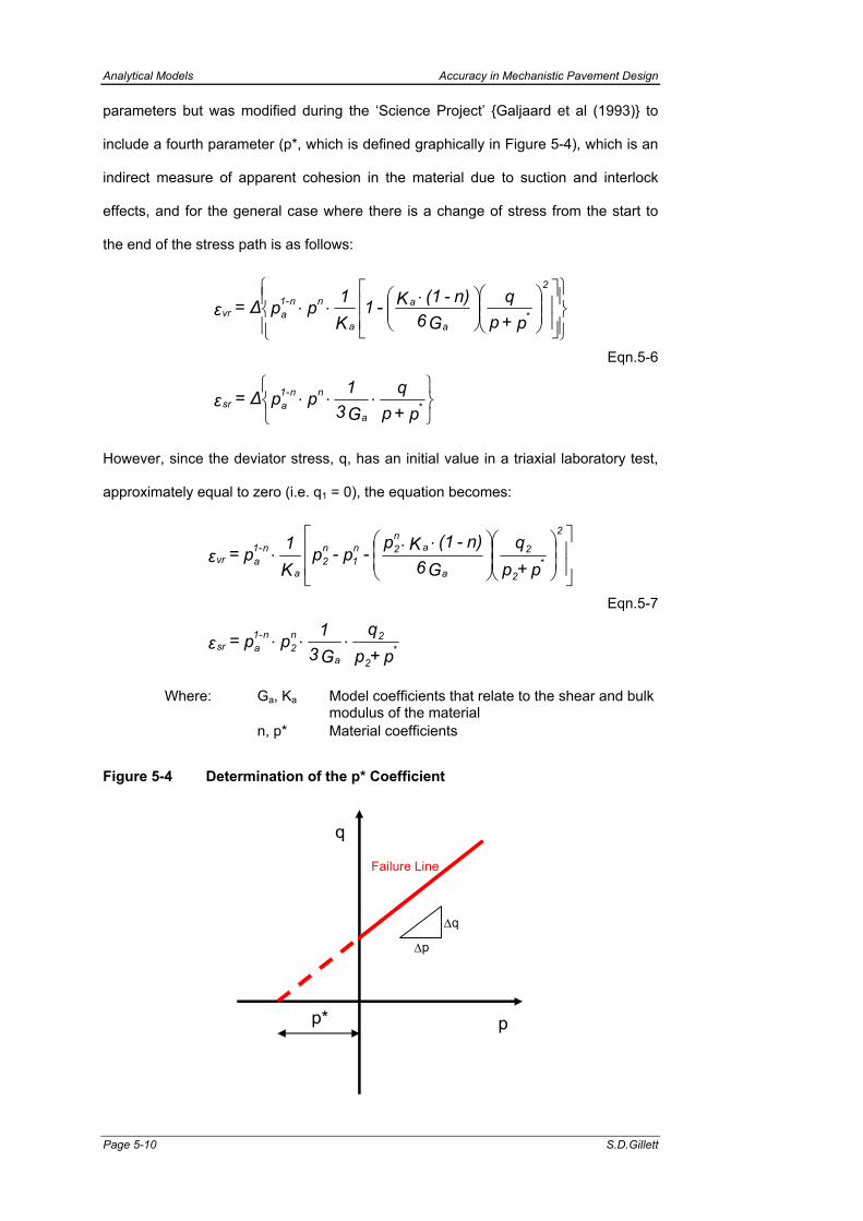
Analytical Models Accuracy in Mechanistic Pavement Design
Page 5-10 S.D.Gillett
parameters but was modified during the ‘Science Project’ {Galjaard et al (1993)} to
include a fourth parameter (p*, which is defined graphically in Figure 5-4), which is an
indirect measure of apparent cohesion in the material due to suction and interlock
effects, and for the general case where there is a change of stress from the start to
the end of the stress path is as follows:
⋅⋅⋅
⋅⋅⋅
p+pq
G31pp∆ = ε
p+pq
G6n)-(1K-1
K1p p∆ = ε
*a
nn-1asr
2
*a
a
a
nn-1avr
Eqn.5-6
However, since the deviator stress, q, has an initial value in a triaxial laboratory test,
approximately equal to zero (i.e. q1 = 0), the equation becomes:
p+pq
G31 p p = ε
p+pq
G6n)-(1Kp
- p- pK1 p = ε
*2
2
a
n2
n-1asr
2
*2
2
a
an2n
1n2
a
n-1avr
⋅⋅⋅
⋅⋅⋅
Eqn.5-7
Where: Ga, Ka Model coefficients that relate to the shear and bulk modulus of the material
n, p* Material coefficients
Figure 5-4 Determination of the p* Coefficient
q
Failure Line
∆q
∆p
pp*

Accuracy in Mechanistic Pavement Design Analytical Models
PhD Thesis Page 5-11
The Mayhew model
When the Boyce equations are analysed in a non-linear parameter evaluation model
the values for the parameters Ga and n for volumetric and shear strain are different for
each. This creates the problem of having two values for the same parameter for the
same model for the same data. Although this difficulty can be overcome by weighting
each relationship, it illustrates the difficulty in fitting the measured material behaviour
(and probably the genuine material behaviour) to the models. This is overcome in the
Mayhew model (see below) by having five parameters instead of the three in the
Boyce model. Again p* was introduced during the ‘Science Project’’ and thus here.
The Mayhew model {Mayhew, (1983)} with 6 parameters is thus:
⋅⋅⋅
⋅⋅
p+pq
G31pp∆ = ε
p+pqβ-1
K1p p∆ = ε
*a
nn-1asr
2
*a
mm-1avr
Eqn.5-8
The shear strain equation is identical to the Boyce model. Again, since the initial
deviator stress (q1) is approximately equal to zero, the equation becomes:
p+pq
G31 p p = ε
p+pq
β p- p- p K1 p = ε
*2
2
a
n2
n-1asr
2
*2
2m2
m1
m2
a
m-1avr
⋅⋅⋅
⋅⋅
Eqn.5-9
Where: β, m Model coefficients
It was noted by Allaart (1989) that these models (Boyce and Mayhew) model the
volumetric strain poorly whereas they predict the shear strain quite well.

Analytical Models Accuracy in Mechanistic Pavement Design
Page 5-12 S.D.Gillett
5.4 SUMMARY
A number of constitutive relationships have been developed in which model
coefficients and subsequent material parameters can be determined. The aim of
these models is to predict the behaviour of the materials under traffic loading. These
vary from simple values determined from simple laboratory testing, for example failure
characteristics yielding relationships between resilient modulus and CBR, to more
complex characteristics which, in practice, are often estimated by simple material
characteristics rather than the results of complex of testing.
The models and corresponding parameters that are to be used for the analysis can be
divided into three categories, namely those:
• For all road construction materials;
• For subgrade soils, and;
• For unbound granular materials.
It is not the intension of this work to develop a model that predicts the behaviour of
road construction materials under traffic loading. As with the pavement design
methodology where limiting strains are correlated to permissible traffic loading the
work of others is used to determine the possible accuracy of laboratory testing and
pavement design using these tools. The main reasons for selecting the models
described above are:
• That a range of models has been selected, from simple to complex models, some
are commonly used for commercial pavement design and other are only used in
research, and;
• The limitations of the software used to analyse the data, certain models are
integrated into the FENLAP {Almeida (1991)} software.

Accuracy in Mechanistic Pavement Design Triaxial Test Apparatus
PhD Thesis Page 6-1
6 TRIAXIAL TEST APPARATUS
6.1 INTRODUCTION
There exist many varieties of triaxial apparatus used for the repeated load testing of
pavement construction materials. These apparatus vary in size and sophistication.
These variations often depend on the characteristics of the material being tested, for
example an apparatus designed to test full sized crushed rock (granular base) will be
much larger than an apparatus used to test fine-grained subgrade soils. The
sophistication of apparatus generally varies with budgets, with some apparatus using
expensive sophisticated different loading systems, deformation measuring devices
and data capture mechanisms, while others use more simple mechanical devices.
6.2 COMMON METHODS OF MEASURING STRAIN ON SPECIMENS IN THE LABORATORY
Spring loaded clamps around the specimen, studs and vanes placed within the
specimen and blocks or targets glued on the membrane have all been used as
reference points between which deformations are measured on the specimen. On
samples of rock or heavily stabilized materials wire resistance strain gauges are
sometimes glued directly on the specimen.
The most common method of measuring specimen deformation is by electronic
measurement devices such as Linear Variable Differential Transformers (LVDT) or
Proximity Transducers (PT). LVDTs have an energising coil wound coaxially with a
receiving coil between which flux is transferred in proportion to the position of a metal
armature that slides along the axis of the coils. The coils are relatively bulky, but the
armature is very thin (diameter about 2 mm) and lightweight. The arrangements for
the support of the LVDTs vary. In general, however, in the case of small softer
specimens a frame supports the weight of the LVDTs whereas the larger, stronger,
specimens are better able to support the weight of the LVDTs. The PTs record the
movement of the specimen without being physically connected to it, therefore an
external frame always supports PTs. PTs measure the change in inductance of a coil
as a ‘target’ piece of foil (fixed to the specimen) is brought into the flux field around the
transducer thus altering its inductance. The response of the PTs is highly non-linear,

Triaxial Test Apparatus Accuracy in Mechanistic Pavement Design
Page 6-2 S.D.Gillett
but a signal conditioner linearises this over a certain specified range of position of the
target from the sensor.
Strictly, these instruments measure the displacement of a specimen under loading;
but as these displacements are used to compute strain (axial and radial) the latter
term will be used here.
6.2.1 Spring-Loaded Rings
The use of spring-loaded rings placed around the specimen to measure axial
displacement is frequently used. The rings are usually constructed from either
aluminium or Plexiglas consisting of two pieces that are hinged on one side and have
a spring-loaded connection on the other. A LVDT (or PT) is placed between the ring
openings and the specimen displacement is measured. Two rings are generally used
in order that axial deformation can be measured between the two rings by either two
or three LVDTs between them. The rings are placed at either the 1/4 or 1/3 points in
from each end of the specimen as discussed earlier. Dehlen (1969) reported using
these rings so that the ring touched the specimen along two short segments. Hicks
(1970) and Barksdale (1972b) also used spring-loaded rings to measure radial
deformation of triaxial specimens.
Tilting of the rings will influence the accuracy of axial strain measurements. This is
probably a result of either barrelling of the specimen or misalignment, accurate
alignment is essential in order that tilting does not occur {Chisolm and Townsend
(1976)}.
It was observed during permanent strain measurements using spring-loaded rings that
the measured strains exhibited a greater scatter after 50,000 load cycles than before
in relation to strain measurements measured in some other less accurate way
{Barksdale (1972b)}. The proposed hypothesis was that the rings underwent small
amounts of slip over an extended number of load applications. Boyce and Brown
(1976) and Pezo et al (1991) also suggest that ring slippage could be a potential
problem in measuring resilient modulus.
Accuracy in Mechanistic Pavement Design Triaxial Test Apparatus
PhD Thesis Page 6-3
To prevent slip between the clamps and the membrane, Chisolm and Townsend
(1976) simply placed a small quantity of epoxy glue on top of each of the clamp
contact points with the rubber membrane. Sweere (1990) used individual LVDT
support blocks glued directly to the membrane. Static tests by Miller, as reported by
Burland and Symes (1982), indicate that relative slip between the specimen and the
enclosing membrane does not occur until near or after failure. The work of Miller
indicates that pasting lightweight clamps or blocks to the membrane should be
satisfactory for the stress levels normally employed in resilient modulus testing.
6.2.2 Studs and Pins
To eliminate the possibility of slip between the radial measuring apparatus and the
specimen, several researchers have placed studs or pins in the specimen {Boyce and
Brown (1976) and Paute et al (1986)}. These studs are embedded within the granular
specimen during specimen manufacture. A second part of the stud is then attached to
the embedded stud through the membrane. Boyce and Brown (1976) consider the
metal studs, which protruded into a granular base material, as simply an artificial
aggregate.
Small cross-shaped vanes have been pushed into a soft cohesive soil to which pins
are attached as reported by Brown (1979). To minimize applying load on these pins,
four LVDTs, which are supported externally, were used to measure the deformation
within the specimen at two locations.
6.2.3 Non-Contacting Sensors
A number of different sensors are available, which do not contact each other including
inductive, optical, ultrasonic, and pneumatic types. Ultrasonic type non-contacting
sensors have a low sensitivity, while pneumatic type non-contacting sensors are large
{Linton et al (1988)}. As a result, neither appears to be suitable for resilient modulus
measurement. However, axial strain on triaxial specimens has been successfully
measured using non-contacting measurement systems including both inductive
proximity gauges and optical scanners. Proximity gauges have been used more
frequently to measure radial deformation for evaluating Poisson's ratio and volume
change, than for axial strain measurement.

Triaxial Test Apparatus Accuracy in Mechanistic Pavement Design
Page 6-4 S.D.Gillett
Inductive Proximity Sensors
Inductive proximity sensors have been successfully used by Dupas et al (1988) to
measure axial strain in gravels and clayey sands. However, for axial measurement
although the proximity sensors themselves are non-contacting, blocks or pins must
still be attached to the specimen, as is the case in LVDT based axial measurement
systems. Thus, if relative displacement is to be measured, then the instrumentation
must be supported by the pins or blocks and hence ultimately by the specimen. If,
however, absolute displacement is used to measure displacement of a reference
point, then only lightweight targets need to be attached to the specimen. During this
work absolute radial measurements were conducted at mid-height of soil specimens
using two opposing PTs fixed to the frame opposite metallic rectangles that were
glued to the specimen at Nottingham and Lisbon.
Although proximity sensors are quite accurate, their use poses some perhaps minor
problems associated with adjusting the sensors to within the correct range when
employed for axial displacement measurement {Barksdale et al (1990)}. Also, they
are moderately expensive.
Optical Scanners
Measurements of displacement during repeated load triaxial test have been performed
using optical scanners, by attaching reflective targets on specimens {Moore et al
(1970), Allen and Thompson (1974), and Knutson and Thompson (1978)}. The
scanner, which is located outside the triaxial cell, optically monitors the movement of
the targets.
The important advantage of using optical scanners over other systems is that only
very light targets are attached to the specimen. If the displacement of each target is
to be measured simultaneously, however, the same number of optical heads is
required as the number of targets. Moore et al (1970) employed a square triaxial cell
chamber to keep from distorting the light beams. A circular cell was used, however, in
the later systems adopted by Allen and Thompson (1974) and Knutson and
Thompson (1978) with the latter reporting no loss in accuracy. Moore reports a high
resolution of the system, being able to make measurements to better than 0.001 mm

Accuracy in Mechanistic Pavement Design Triaxial Test Apparatus
PhD Thesis Page 6-5
over a 1.8 mm range. Optical scanner heads, unfortunately, are expensive and are
probably not suitable for routine testing.
Pore Pressure Measurement
Most triaxial testing equipment measures pore pressures at the base of the sample,
and because some end restraint will always be present, the measured pore pressure
will not be representative. Some researchers, such as Sangrey et al (1969), used
very low frequencies of loading to allow time for pore pressure equalisation. Others,
such as Koutsoftas (1978), allowed time after faster cyclic loading for the pore
pressure to equalise. In either case the end effects will still distort the recorded pore
pressure but the second method has the advantage of testing at representative
frequencies or rates of loading. It seems likely that the most accurate pore pressure
measurements will be from a centre probe in the relatively uniform central section of
the sample before pore pressure equalisation has taken place Hight (1983), assuming
that the transducer itself does not cause any significant effects.
6.3 APPARATUS AND EQUIPMENT USED DURING THIS WORK
The following section contains a description of each of the participating laboratory’s
test apparatus and their corresponding instrumentation systems.
6.4 UNIVERSITY OF NOTTINGHAM
Two repeated load triaxial apparatus were used in this work at the School of Civil
Engineering at the University of Nottingham, one to test subgrade soils and the other
to test unbound granular base materials. These are shown in Photograph 6-1.
6.4.1 Variable Confining Pressure Apparatus (150 mm x 76 ∅mm) for Testing of Subgrade Soils
The Apparatus
The servo controlled hydraulic triaxial testing facility was first developed in 1971 for
testing fine grained soils and has since undergone a number of modifications {Loach
(1987)}. The apparatus is contained in an air-conditioned laboratory and consists of a
loading frame with two hydraulic actuators, one for axial load and the other for cell
pressure. A pump supplies hydraulic power, at a normal operating pressure of

Triaxial Test Apparatus Accuracy in Mechanistic Pavement Design
Page 6-6 S.D.Gillett
14 MPa. The control system permits the user to cycle both axial and confining
pressure. The apparatus is illustrated in Figure 6-1.
Photograph 6-1 Apparatus at Nottingham
Variable Confining Pressure Apparatus (150 mm x 76 ∅mm) for Testing of Subgrade Soils
Variable Confining Pressure Apparatus (300 mm x 150 ∅mm) for Testing of Unbound Granular Materials
The axial load is applied to the specimen by connecting the load ram in the triaxial cell
directly to the hydraulic actuator, thus tension can be applied axially. The axial
loading system has a load capacity of approximately 12 kN, which allows a pressure
of 2500 kPa to be applied on a specimen.
Silicone oil confining fluid is used in the triaxial cell (Dow Corning 200/20 cs) since it is
non-conductive and therefore does not interfere with the electronic instruments. The
confining pressure is applied by connecting the hydraulic actuator to a piston, which
acts on the silicone oil to a maximum pressure of about 400 kPa. The feedback
transducer is a strain gauged diaphragm pressure transducer, located in the cell. The
servo control system compares the control signal with the feedback signals provided
by the outputs of the axial load cell and the cell pressure transducers. The electronic
system allows control of the cycling of both the confining stress and the deviator

Accuracy in Mechanistic Pavement Design Triaxial Test Apparatus
PhD Thesis Page 6-7
stress by limits of stress or by limits of deformation. The triaxial cell contains a
specimen 150 mm high with a 76 mm diameter.
Specimen Manufacture
The fine-grained material was conditioned (by adding water or drying) and mixed to
the required moisture content. The material was compacted into a steel mould of
diameter 76 mm using a rammer weighing 4.54 kg (BS1377 Modified Proctor
Hammer). The number of layers of material and the number of blows was determined
by a method of trial and error until the required density at the specified moisture
content was attained. Alternatively, some specimens have been manufactured by
placing the mould on a vibratory table, placing the material in five layers in the mould
and applying a surcharge to each layer for a fixed period of vibration. This method is
described by Boyce and Brown (1976).
Instrumentation
An instrumentation support frame is placed around the specimen and the location of
the axial and radial points of measurement marked on the specimen. Four axial
locating cruciform vanes are pressed into the specimen at 1/3 and 2/3 of the specimen
height and two metallic rectangles (25 x 35 mm) (aluminium foil) are fixed to the
specimen by glue adhesion, at the mid-height, for the radial measurement. This is
shown in Figure 6-1. Two 5 mm wide nylon gauze strips are placed vertically along
the length of the specimen, to distribute the pore pressure between the top and the
bottom of the specimen. A latex membrane is placed over the specimen and fixed by
two rubber ‘O-rings’ to the top and bottom platens. A pin is screwed through the
membrane into each locating vane and the LVDT armature connected to the pin. The
specimen is then placed between upper and lower platens in the cell and the frame is
fixed to the base of the cell. Four LVDTs (Figure 6-1) are connected to the frame and
to each of the pins (cruciform vanes). The difference between the reading of
deformation of the upper and lower LVDT in each pair allows axial strain to be
computed. The radial deformation is measured at mid-height of the specimen using
two opposing PTs fixed to the frame opposite the metallic rectangles.

Triaxial Test Apparatus Accuracy in Mechanistic Pavement Design
Page 6-8 S.D.Gillett
The triaxial cell is sealed, placed in the loading frame and filled with fluid. The triaxial
cells are fitted with castors to minimise the need to lift and carry the cells and limit
specimen disturbance.
6.4.2 Variable Confining Pressure Apparatus (300 mm x 150 ∅mm) for Testing Unbound Granular Materials
The Apparatus
This equipment was first developed at Nottingham in 1974 in order to provide a test
facility with which to study the mechanical properties of unbound granular materials
used in pavement construction. Facilities to cycle both the confining stress and the
deviator stress were provided, to approximately represent the effects of repeated
wheel loading in the pavement. The equipment allows for testing materials with a
maximum grain size of 30 mm particle size.
The main components of the triaxial cell and servo-hydraulic loading systems for
deviator and confining stresses are shown in Figure 6-2. The test specimen is housed
in a sealed, pressurised triaxial cell. Silicone oil is once again used as the cell fluid.
Axial load is applied to the specimen by a hydraulic actuator and monitored by a load
cell. Confining stress is applied through the silicone fluid surrounding the test
specimen. A second hydraulic actuator loads a piston in a pressure cylinder that
controls the fluid pressure. A pressure sensor in the triaxial cell monitors the
pressure. The axial loading system has a load capacity of approximately 20 kN. This
allows deviator stresses in the range 1200 kPa to be applied on 150 mm diameter
specimens. A cell pressure of up to 400 kPa can be applied.

Accuracy in Mechanistic Pavement Design Triaxial Test Apparatus
PhD Thesis Page 6-9
Figure 6-1 University of Nottingham - Variable Confining Pressure Apparatus (150 mm x 76 ∅mm)
Specimen Manufacture
The specimen is prepared in a four-piece aluminium split mould into which an inner
latex membrane is held using a vacuum. Four “locating studs” are attached to the
inner membrane. The test material is then placed in layers, each being subjected to a
programme of vibration, while a small surcharge load is applied, thus enabling the

Triaxial Test Apparatus Accuracy in Mechanistic Pavement Design
Page 6-10 S.D.Gillett
density to be controlled. Once compaction is complete a top platen is placed on the
specimen and the membrane is sealed to it using ‘O-rings’. Then an internal vacuum
is applied to the specimen thus allowing the mould to be dismantled and the specimen
to be transferred to the cell base. A second outer latex membrane is placed on the
specimen in case the first was punctured during the compaction.
Figure 6-2 University of Nottingham - Variable Confining Pressure (300 mm x 150∅ mm)

Accuracy in Mechanistic Pavement Design Triaxial Test Apparatus
PhD Thesis Page 6-11
Instrumentation and Data Capture
Four studs are used which allow two independent radial strain measurements to be
made. The studs are typically placed over the central 150 mm of the specimen height,
at ¼ and ¾ of the specimen height (to avoid any end effects) at 180° to one another
as shown in Figure 6-2.
Two small LVDTs are attached between the studs (as above) to measure the axial
movement during loading. Flexible strain-gauged rings are also attached to the
locating studs, which measure the radial movement of the specimen under loading.
These rings are made from casting epoxy (Araldite resin MY 778 resin HY 956) and
weigh approximately 25 g.
6.5 LABORATÓRIO NACIONAL DE ENGENHARIA CIVIL
The Laboratório Nacional de Engenharia Civil has two repeated load triaxial
apparatus as shown in Photograph 6-2.
Photograph 6-2 Apparatus at Lisbon
Variable Confining Pressure Apparatus (150 mm x 76 ∅mm) for Testing of Subgrade Soils
Constant Confining Pressure Apparatus (600 mm x 300 ∅mm) for Testing Unbound Granular Materials

Triaxial Test Apparatus Accuracy in Mechanistic Pavement Design
Page 6-12 S.D.Gillett
6.5.1 Variable Confining Pressure Apparatus (150 mm x 76 ∅mm) for Testing of Subgrade Soils
For the repeated load triaxial testing of soils the Laboratório Nacional de Engenharia
Civil uses an apparatus very similar to that at the University of Nottingham, which was
manufactured by the University. The loading characteristics and specimen
manufacture are identical to those of the Nottingham apparatus. The computer
control and data acquisition hardware used is a Hewlett Packard 3852A data
acquisition unit and a Hewlett Packard 900 series 300 computer. The data acquisition
software was written and is maintained by the Laboratory {Gillett (1994)}.
6.5.2 Constant Confining Pressure Apparatus (600 mm x 300 ∅mm) for Testing Unbound Granular Materials
This apparatus was developed by Nunes and Gomes Correia (1991), conceptually
based on a triaxial cell used for testing rock-fills by Veiga Pinto (1983). It was
developed for the testing of full sized single sized granular material used for railway
ballast in Portugal. During this project it was modified to conduct repeated load tests
on unbound granular materials of up to 40 mm grading. The triaxial specimen height
is 600 mm with a diameter of 300 mm.
The Apparatus
The loading frame is constructed from standard mild steel sections of sufficient
strength to withstand loading of up to 50 kN. The deviator stress is applied by means
of a hydraulic jack attached to the loading frame, which applies a load to the top
platen. Pressure to the jack is applied by means of an ENERPAC BVE-31 pump
apparatus and an ENERPAC BIC-93 program control centre. This system can apply a
maximum force of 25.7 kN, which imposes a maximum deviator stress on a specimen
of 300 mm diameter of about 330 kPa. The maximum realistic operational frequency
of loading, i.e. load-on load-off to load on again, of this system is about 0.5 to 0.6 Hz.
The confining pressure is applied by means of a CENCO HYVAC7 vacuum pump that
can apply a maximum vacuum of 70 kPa. The apparatus is shown schematically in
Figure 6-3.

Accuracy in Mechanistic Pavement Design Triaxial Test Apparatus
PhD Thesis Page 6-13
Figure 6-3 Laboratório Nacional de Engenharia Civil - Constant Confining Pressure Apparatus (600 mm x 300 ∅mm)
Specimen Manufacture
A rugged rubber membrane is placed inside a steel split mould of two halves and
three sections high and the material is compacted in ten layers of approximately 10 kg
(for materials having a specific gravity of around 2.65) and 60 mm height using a

Triaxial Test Apparatus Accuracy in Mechanistic Pavement Design
Page 6-14 S.D.Gillett
vibration hammer. In this manner the correct density is attained for specified moisture
contents.
Once the specimen has been compacted and the split mould removed the rubber
membrane is peeled off. This is done because of the possible confining pressure
applied by the rubber membrane. The rubber membrane is replaced by a 0.3 mm
thick oversized plastic membrane, which is made up of a plastic sheet wrapped
loosely around the specimen and sealed with plastic tape and silicone sealant.
Although this membrane is not very extensible, it is sufficiently oversize to allow the
specimen to expand axially and laterally and does not apply a significant confining
pressure to the specimen.
A vacuum is applied inside the membrane to simulate the confining pressure, thus
there is no triaxial cell around the specimen as is usual with triaxial apparatus.
Applying a sub-atmospheric pressure to the inside of the triaxial specimen simulates
the confining stress. An advantage of not having a pressure cell is that the
transducers for measuring the strains remain accessible during the test, thus small
range differential transducers may be used (and manually adjusted should they go out
of range).
Instrumentation and Data Capture
Axial strains are measured by means of an LVDT on the top platen and by two glue-
on LVDT holders at ¼ and ¾ positions each on opposite sides of the specimen. The
radial deformation is measured by means of a ‘String of Wheels’ wrapped around the
specimen at mid-height, while a LVDT measures the increase or decrease of the
circumference of the specimen and thus the radial deformation. The instrumentation
is shown in more detail in Figure 6-3.
This system was based on a prototype utilised at The University of California at
Berkeley. A steel cable is threaded through ten sets of wheels and attached to a
LVDT holder at each end. A LVDT then measures the increase in the circumference
of the specimen and thus the radial deformation. Each set of wheels comprises a pair
of wheels on an axle through which a steel cable of diameter 2 mm, coated in plastic,
is threaded. These axles are not fixed to the cable, thus the cable may move through

Accuracy in Mechanistic Pavement Design Triaxial Test Apparatus
PhD Thesis Page 6-15
the axles. The ends of the cable are attached to the LVDT holders. The ‘String of
Wheels’ is then wrapped around the specimen and held together by two fairly stiff
elastic bands, and the wheels are manually spaced around the specimen.
The method of data capture is by means of pen plotters. A load cell, manufactured by
Automation Industries (TDC 205) between the loading jack and the top platen sends a
signal to an XY plotter, and thus the load is recorded and monitored as it is varied
manually, The LVDTs send signals via a wheatstone bridge to pen recorders. The
vacuum is controlled by means of a bleed and is monitored manually at two pressure
gauges one at the pump and the other through the top platen. This method of load
control and data capture although functional is very time consuming and prone to
operator errors.
6.6 LABORATOIRE REGIONAL DES PONTS ET CHAUSSÉES
The Laboratoire Regional Des Ponts et Chaussées has two repeated load triaxial
apparatus. One at Saint Brieuc for testing granular material, shown in Photograph
6-3, and the other for testing subgrade soils at Clermont Ferrand.
The Apparatus
This triaxial cell is based on the standard equipment manufactured by Wykeham
Farrance with an adapted base to house 70 mm diameter specimens. The extra
space between the specimen and the cell is used to mount the internal instruments in
order to measure the deformations of the specimen.
In the cell top there is a Druck PDCR 22 transducer used to accurately monitor the cell
pressure. The cell base has been modified to allow access for the cables of the
measuring instruments, which are inside the cell. Both the axial load and the
confining pressure systems are based on those developed at the University of
Nottingham. The cell pressure is applied to the specimen by means of non-
conducting silicon oil in the cell. This is schematically shown in Figure 6-4.

Triaxial Test Apparatus Accuracy in Mechanistic Pavement Design
Page 6-16 S.D.Gillett
Photograph 6-3 Apparatus at Saint Brieuc
Variable Confining Pressure Apparatus (320 mm x 160 ∅mm) for Testing Unbound Granular Materials
6.6.2 Variable Confining Pressure Apparatus (150 mm x 70 ∅mm) for Testing of Subgrade Soils
Specimen Manufacture
The specimens are compacted in five layers, in a split mould, that is lined with a latex
membrane. Each layer is compacted by a vibrating full faced surcharge to produce
the required height and thus dry density. The anchors for the axial and radial
measuring devices are attached to the mould and the material compacted around
them. For dry sand, the material is compacted in a single layer on a vibrating table
(frequency 50 Hz and amplitude of 0.42 mm) with a surcharge of 10 kPa. For moist
soils, the moisture content is varied to achieve the correct density and, subsequently,
the specimen is dried until the correct moisture content is attained. Some work was
conducted on the uniformity of the specimen as a function of layers {Gomes Correia
(1985)} and a specimen compacted in five layers was found to provide a uniform
specimen when tested with a nuclear density method.

Accuracy in Mechanistic Pavement Design Triaxial Test Apparatus
PhD Thesis Page 6-17
Instrumentation and Data Capture
The axial deformation is measured using four LVDTs diagonally opposite each other
on the specimen, two in each plane at 1/3 and 2/3 the specimen height. Each LVDT is
supported by a frame and attached to the specimen by means of a probe, anchored in
the specimen, in a similar manner to the Nottingham cruciform vane. This is shown in
Figure 6-4.
The radial deformation is measured by two LVDTs, supported by a frame, diagonally
opposite each other in each plane at mid specimen height. On the end of the core of
the LVDT is a flat disc (15 mm in diameter) which is held by a light spring to a dome
that is attached to an anchor embedded in the specimen. This allows the radial
deformation to be measured despite axial displacement of the dome.
A Hewlett Packard series 200 computer (HP 9816S) processes the recorded data. All
the equipment and software used for the data acquisition and processing was
developed and is maintained by LRPC. The data acquisition system records the
movement of the four axial transducers and four radial transducers. The number of
measurements monitored by the data acquisition is limited to 50 cycles, under the
maximum frequency of loading allowed by the apparatus.
The Apparatus
This repeated load triaxial apparatus was developed for the study of the behaviour of
unbound granular materials. The specimen size is 320 mm high and 160 mm
diameter. The major difference between this apparatus, and those used by other
participating laboratories, is that the loading is pneumatically powered. The drainage
is controlled at both ends of the specimen through porous plates. A load cell is
positioned on the top platen thus frictional effects between the loading rod and cell are
avoided and the cell pressure is measured by means of a pressure transducer in the
cell. The maximum cell pressure is 500 kPa.
The maximum compressive force on the loading frame is 15 kN, which is 745 kPa on
a specimen of diameter 160 mm. The pneumatic jack, applying the axial load, and the
cell pressure cylinder are supplied by two different circuits, as illustrated by Figure 6-5.
For each of them, two sensitive pressure regulators give the maximum and the

Triaxial Test Apparatus Accuracy in Mechanistic Pavement Design
Page 6-18 S.D.Gillett
minimum value of the pressure of the cycle. On each circuit, an electro-pneumatic
distributor connects the line of the cell (or the jack) alternately to the maximum or
minimum pressure.
Figure 6-4 Laboratoire Regional Des Ponts et Chaussées - Variable Confining Pressure Apparatus (150 mm x 70 ∅mm)

Accuracy in Mechanistic Pavement Design Triaxial Test Apparatus
PhD Thesis Page 6-19
6.6.3 Variable Confining Pressure Apparatus (320 mm x 160 ∅mm) for Testing Unbound Granular Materials
The two distributors are guided by a current impulse delivered by a timing unit, which
provides the time of loading and unloading. The load and cell pressure signals
(shown on an oscilloscope) are adjusted to approximate a sinusoidal shape by
delivery control valves. In variable confining pressure mode, the frequency of the
loading is 0.5 Hz. In constant confining pressure mode, the frequency is 1 Hz.
Specimen Manufacture
A latex membrane and the attached anchors for the axial and radial measuring
devices are placed inside a split mould The specimen is compacted in a single layer,
by a full-faced surcharge, while the mould is vibrated, to a specified height and thus
dry density. In certain cases the moisture content can be measured to achieve the
correct density and subsequently dried. The density of each specimen is checked for
uniformity with a radiometric device.
Instrumentation and Data Capture
The axial movement is measured by three LVDTs positioned at 120° to one another,
attached between the anchors at 1/3 and 2/3 of the specimen height. These LVDTs are
held in place by an aluminium hoop and are supported by the specimen. Three
LVDTs, at 120° to one another, measure the radial movement. These are mounted on
a Perspex ring at mid-height of the specimen. On the end of the core of the LVDT is a
flat disc that is held, by a light spring, to a dome that is attached to the anchor
embedded in the specimen. This allows the radial deformation to be measured
despite axial displacement of the dome. This is shown graphically in Figure 6-5. All
data is collected by means of a computerised data acquisition system.
During tests on unbound granular materials, to maintain a constant air pressure within
the specimen, non-woven geotextile discs, treated with a silicone emulsion are
interposed between the specimen and the porous stone discs. Permeable to air,
these discs allow the interstitial air to be connected with the atmosphere, but allow the
pore water suction to be independently controlled by using ceramic discs at the base
of the specimen with an appropriate air pressure entry.

Triaxial Test Apparatus Accuracy in Mechanistic Pavement Design
Page 6-20 S.D.Gillett
Figure 6-5 Laboratoire Regional Des Ponts et Chaussées -Variable Confining Pressure Apparatus (320 mm x 160 ∅mm)
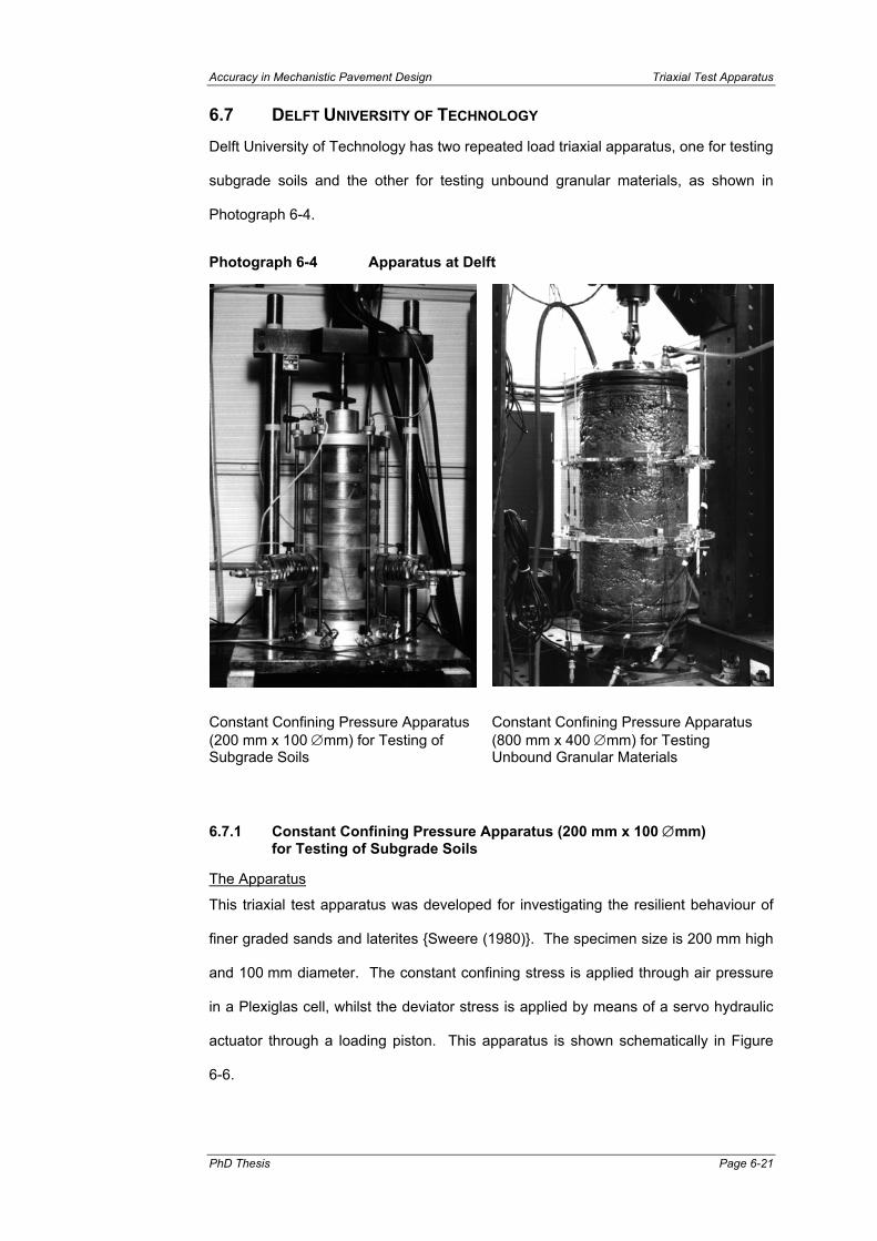
Accuracy in Mechanistic Pavement Design Triaxial Test Apparatus
PhD Thesis Page 6-21
6.7 DELFT UNIVERSITY OF TECHNOLOGY
Delft University of Technology has two repeated load triaxial apparatus, one for testing
subgrade soils and the other for testing unbound granular materials, as shown in
Photograph 6-4.
Photograph 6-4 Apparatus at Delft
Constant Confining Pressure Apparatus (200 mm x 100 ∅mm) for Testing of Subgrade Soils
Constant Confining Pressure Apparatus (800 mm x 400 ∅mm) for Testing Unbound Granular Materials
6.7.1 Constant Confining Pressure Apparatus (200 mm x 100 ∅mm) for Testing of Subgrade Soils
The Apparatus
This triaxial test apparatus was developed for investigating the resilient behaviour of
finer graded sands and laterites {Sweere (1980)}. The specimen size is 200 mm high
and 100 mm diameter. The constant confining stress is applied through air pressure
in a Plexiglas cell, whilst the deviator stress is applied by means of a servo hydraulic
actuator through a loading piston. This apparatus is shown schematically in Figure
6-6.

Triaxial Test Apparatus Accuracy in Mechanistic Pavement Design
Page 6-22 S.D.Gillett
A load cell is incorporated inside the triaxial cell, thereby eliminating load measuring
errors caused by the friction between the loading piston and the top of the triaxial cell.
Specimen Manufacture
The specimen is compacted in six layers in a split mould with a rubber membrane
placed inside it using a tamping compaction device developed at TUDelft.
Instrumentation and Data Capture
Axial deformation is measured by an LVDT connected to the loading piston outside
the triaxial cell and thus the end effect of the contact of the specimen and the platens
is not eliminated. Radial deformation of the triaxial specimen is measured by three
non-contacting PT sensors, which are mounted through the Plexiglas cell on a
horizontal plane at mid-height of the specimen.
Figure 6-6 Delft University of Technology - Constant Confining Pressure Apparatus (200 mm x 100 ∅mm)
6.7.2 Constant Confining Pressure Apparatus (800 mm x 400 ∅mm) for Testing Unbound Granular Materials
The Apparatus
This apparatus was developed in the 1980s for testing of unbound granular materials
for roads {Sweere (1990)}. Due to the large specimen size of 800 mm in height and

Accuracy in Mechanistic Pavement Design Triaxial Test Apparatus
PhD Thesis Page 6-23
400 mm in diameter it was necessary to try and circumvent the need for a triaxial cell
around the specimen. In a similar method to that used by LNEC a sub-atmospheric
pressure is applied within the membrane to the triaxial specimen. In this manner a
confining stress is simulated.
The specimen is enclosed by a double membrane, which has an airtight connection to
the bottom and top platens using ‘O-rings’ and grease. A constant vacuum is applied
to the specimen through a bore in the top platen, while another bore in the top platen
is connected to a vacuum reducer providing a constant controlled bleed. The
hydraulic system can apply 100 kN (800 kPa) repeatedly, at frequencies of up to
10 Hz. This apparatus is shown in Figure 6-7.
Specimen Manufacture
The material is compacted in a split mould lined with a membrane made from plastic
of 0.4 mm thickness, which are welded into on oversize barrel shape to allow the
specimen to expand in a radial direction under load. The material is divided into 8
portions compacted into the mould with a heavy tamper. A full face compactor plate is
applied to the second, fourth, sixth and eighth layers for 30 minutes each using a
haversine load of 7 Hz frequency and 40 kN amplitude superimposed on a 10 kN
static load. Due to the large amount of material required to make a specimen it was
found not to be possible to control the moisture content accurately.
Instrumentation and Data Capture
LVDTs mounted on two Plexiglas rings surrounding the specimen, at positions of one
third and two thirds of the height, and measure the axial and radial deformations of the
specimen. Plastic blocks glued to the membrane support these rings, thus the
specimen supports the instrumentation. Four vertically mounted LVDTs between the
rings measure axial deformations, while two horizontally mounted proximity
transducers are used to measure the radial deformations as the rings open and close.
This is shown in detail in Figure 6-7.

Triaxial Test Apparatus Accuracy in Mechanistic Pavement Design
Page 6-24 S.D.Gillett
Figure 6-7 Delft University of Technology - Constant Confining Pressure Apparatus (800 mm x 400 ∅mm)

Accuracy in Mechanistic Pavement Design Triaxial Test Apparatus
PhD Thesis Page 6-25
6.8 COMPARISON OF THE APPARATUS AND INSTRUMENTATION SYSTEMS
In total eight apparatus were used in the five laboratories and seven of these differ to
some degree. The specimen diameter varies from 70 mm to 400 mm between the
laboratories as illustrated (diagrammatically) in Figure 6-8.
In all apparatus a load cell attached to the upper loading piston measures the axial
load. It is noted that the measurement of the actual loads applied to the specimen
should be made inside the cell, where relevant, thus avoiding the friction caused by
the plunger and the cell top, which can be quite substantial since a good seal is
required due to pressurisation of the cell.
There are two methods of applying radial stress, the first, used on the smaller
specimens, is to apply a confining pressure within the cell using either non-conductive
silicone oil (or air in the case of LRSB). In general these systems allow the radial
stress to be applied cyclically. The second method is to apply a constant vacuum to
the specimen, which is enclosed in an airtight membrane attached to the top and
bottom platens, using a vacuum pump. The second system does not allow repeated
loading of the radial stress.
To obtain representative strain values instrumentation is required which will be affixed
to the specimen somewhat remote from the ends and which will measure deformation
longitudinally and radially as the specimen is loaded. Figure 6-8 indicates the
instrumentation systems used at each laboratory on their repeated load triaxial
equipment and these are summarised in Table 6-1. There are obvious differences
between these instrumentation systems but primarily size and weight are important.
Since the influence of the weight of the instrumentation on the specimen is more
critical on the smaller specimens these tend to have a method of supporting the
instrumentation remote for the specimen whereas the larger, stronger, specimens are
capable of supporting the instrumentation on the specimen.

Triaxial Test Apparatus Accuracy in Mechanistic Pavement Design
S.D.Gillett Page 6-26
Figure 6-8 Instrumentation Layout for the Repeated Load Triaxial Apparatus
LVDT
LRCF(small)
140mm x 70mmSoils
LNEC/UNOT(small)
145mm x 75mmSoils
DUT(large)
800mm x 400mmUGM
LVDT
LVDT
LVDT LVDT
LVDT
PT - Proximity TransducerSOW - String of WheelsLVDT - Linear Variable Displacement Transformer
Legend:
4 LV
DT
2 RingsPT
RingPT
LNEC(large)
600mm x 300mmUGM
SOWLVDT
3 LV
DT
SOWLVDT
RingPT
LRSB(large)
320mm x 160mmUGM
3 LV
DT
LVDTLVDT
LVDT LVDT
3
LVDT
PT
LVDT
LVDT
Unott(large)
300mm x 150mmUGM
2 RingsPT
4 LV
DT
4 LV
DT
Hoop
SG
HoopSG
PT
3
PT2PT
DUT(small)
200mm x 100mmSoils
LVDTPT
PT
LVDT
LVDT LVDT
LVDT
LVDT
LVDT
LVDT
LVDT
LVDT
LVDT
LVDT
Fine Grained Subgrade Soil Coarse Graded Unbound Granular MaterialConfining Pressure by Vacuum
LVDT LVDT
2 LV
DT

Accuracy in Mechanistic Pavement Design Triaxial Test Apparatus
PhD Thesis Page 6-27
The three apparatus designed for testing fine-grained subgrade soils (LRCF, UNOT
and LNEC) are almost identical; however there is more difference in the remaining
four apparatus (which are designed for testing larger unbound granular base
material). The largest two specimens (LNEC and DUT) provide a confining pressure
by internal vacuum rather than by a pressure chamber and thus the size of their on-
sample instrumentation systems are less restricted.
6.8.1 Instrumentation Fixing Methods
Axial Strain Measurement Systems
In all cases, the axial strains were measured using LVDTs as shown in Table 6-1. In
the case of the smaller systems (LRCF, LNEC/ UNOT), two pairs of LVDTs bodies are
supported on either side of the specimen, on a frame fixed to the base plate of the
triaxial cell, and only the armatures are carried by the sample. Small cruciform vanes
are inserted into the wall of the triaxial specimen vertically above each other, at the
quarter points (LRCF) and the third points (UNOT/ LNEC) of specimen height, and the
membrane is placed over the specimen. A pin is fixed to the vane, by piercing the
membrane, and also to the armature of the LVDT. A disadvantage of this
arrangement is that the axial strain reading comes from the difference between two
measures and thus includes a greater error probability than if read as one
measurement. However, since the total weight of this system is <5 g, this minimises
the stress imposed by the weight of the on-sample instrumentation and thus the
likelihood of specimen deformation.
The smaller apparatus at DUT does not use on-sample instrumentation for axial strain
measurement but measures the axial deformations from the top platen but this has
been shown to give erroneous results due to end effects between the specimen and
the platens {Sweere (1990)}.
For three of the four larger unbound granular material systems one LVDT was made
to span between fixings at either the third (LRSB, DUT large) or quarter points (UNOT
large). This is because the stronger specimens are assumed to be more able to carry
the weight of the complete instrument.

Triaxial Test Apparatus Accuracy in Mechanistic Pavement Design
Page 6-28 S.D.Gillett
Table 6-1 Summary of Triaxial Apparatus of the Participating Laboratories
Specimen Size (mm)
Strain Measurement Loading System Laboratory
Height Diameter Axial Radial Deviatoric Confining
LNEC1,6 150 76 2 pairs LVDT on studs3
2 proximity transducers
Servo-hydraulic
Servo-hydraulic
LNEC7 607 308 2 LVDTs on glued blocks
‘String of Wheels’
Servo-hydraulic
Partial vacuum, non-repetitive
UNOT6 150 76 2 pairs LVDT on studs3
2 proximity transducers
Servo-hydraulic
Servo-hydraulic
UNOT7 300 150 2 LVDTs on studs
2 flexible hoops on studs
Servo-hydraulic
Servo-hydraulic
LRCF2,6 140 70 2 pairs LVDT on studs3
2 pairs LVDT to studs5
Servo-hydraulic
Servo-hydraulic
LRSB7 320 160 3 LVDTs sprung to studs
3 LVDTs to domed studs5
Pneumatic Pneumatic
DUT2,6 200 100 External LVDT
3 proximity transducers5
Servo-hydraulic
Hydraulic, non-repetitive
DUT7 800 400 4 LVDTs between hoops
2 calliper hoops on glued blocks4
Servo-hydraulic
Partial vacuum, non-repetitive
Notes: 1 Can measure and control pore suctions 2 Can measure pore suctions 3 Each LVDT body is mounted on a fixed frame.
Axial strain is computed from the difference between readings of a pair mounted above each other
4 Each calliper touches the specimen at two, opposite, points 5 Adjustable through cell wall during testing 6 Primarily for fine-grained subgrade soils 7 Primarily for base and subbase aggregates
For the larger unbound granular material specimens at UNOT and LRSB studs are
placed in the specimen’s material prior to compaction. Again, a membrane is placed
over the specimen and a pin pierces the membrane, which is then sealed. For the
much larger triaxial specimens at LNEC and DUT the fixing is provided by a block,
glued to, but not penetrating, the plastic membrane. Glueing allows easy attachment
of the fixing after the sample has been compacted and placed in position, ready for

Accuracy in Mechanistic Pavement Design Triaxial Test Apparatus
PhD Thesis Page 6-29
testing. Also, there is no possibility of the fixing affecting the local quality of the
compaction of the material, which may cause unreliability with strain measurements
when embedded fixings are utilised.
On the LRSB apparatus the LVDTs have cones at each end that are spring-loaded
into a cup attached to the fixing. This approach enables the sensor to measure the
spacing between two points (which are arranged to be in the periphery of the
specimen) with minimal influence of the rotation of the fixings that might occur due to
the influence of individual aggregate particles, for example.
The larger UNOT apparatus has simple threaded rods to which the LVDTs are
attached. It has the advantage of greater simplicity but the influence on axial strain
measurement of rotation of the fixings may not be negligible. The large DUT
apparatus clamps the LVDT to a Plexiglas ring that is fixed to the glue-on blocks. A
rod with two universal joints extends the LVDTs armature, which allows for any lack of
coaxiality in the fixing points.
Radial Strain Measurement
Three of the apparatuses use proximity transducers to measure radial strain as shown
in Table 6-1, in which a piece of aluminium foil is placed between specimen and
membrane as a ‘target’ (LNEC, UNOT and DUT small). For radial strain
measurement the smaller apparatus at LRCF and larger apparatus at LRSB use
embedded studs similar to those used by LRSB for axial strain measurement fixings
into which domed nipples are screwed. Spring-loaded LVDTs set in the cell wall have
plate tips that rest on the domes thus measuring the radial movement allowing some
longitudinal movement. These are positioned at one third and two thirds of specimen
height and at 180° (LRSB) and 120° (LRCF) spacing around the specimens.
On the small triaxial apparatus at UNOT and LNEC these transducers are supported
on the same frame that carries the bodies of the axial LVDTs. Strains are thus
measured only at mid-height of the specimen with two opposing sensors. At DUT
they are held in the cell wall of the smaller apparatus at mid-height of the specimen
(with 3 sensors at 120° pitch around the specimen) but, in the larger DUT apparatus,
are affixed to a calliper Plexiglas ring that rests on some of the glue-on blocks. A

Triaxial Test Apparatus Accuracy in Mechanistic Pavement Design
Page 6-30 S.D.Gillett
proximity transducer acts across the opening jaws of the hinged callipers. In that
apparatus there are two such rings enabling the radial strain to be assessed at both
one third and two thirds of the specimen height.
In the large LNEC apparatus a necklace-style ‘string-of-wheels’ is used at mid height
with a LVDT as the active part across an opening. This ‘necklace’ comprises a steel
cable, drawn tight around the specimen by a sprung link across the opening in the
‘necklace’, on which are arranged 12 ‘single-axle bogies’. The wheels thus keep the
cable a constant distance from the specimen or, strictly speaking, the membrane
necessitating an increased opening in the ‘necklace’ as the specimen expands. An
LVDT is placed across this opening to monitor strain.
The large UNOT apparatus uses epoxy resin hoops fitted to the same fixings that hold
the axial LVDTs, thus providing strain measurements at one quarter and three
quarters of specimen height. The hoops are strain-gauged using resistance wire. As
the sample expands the curvature of the hoop changes and this is sensed by a
change in the resistance of the gauges.
Because the specimen did not require a membrane the effect of a membrane and the
glue-on fixing methods used at LNEC and DUT on their large vacuum confining
pressure apparatus was not tested. In a separate study, Karaşahin (1993) compared
the performance of the UNOT LVDT and epoxy hoop system, which is supported on
inserts or studs, with the same instruments supported on glue-on fixings. He
observed that, while the confining stress remained constant, the two instruments gave
comparable readings. However, if the confining stress changed the two systems gave
very different results with much higher radial strains and lower axial strains with
increasing confining stress when glue-on fixings were used.
Cheung (1994) tested a smooth-sided rubber specimen to check whether glue-on
instruments might misread due to slipping of the membrane. Even when applying only
a partial vacuum confining pressure of 10 kPa, he detected no significant effect on
resilient axial or radial strain measurements.
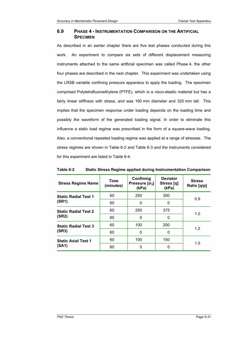
Accuracy in Mechanistic Pavement Design Triaxial Test Apparatus
PhD Thesis Page 6-31
6.9 PHASE 4 - INSTRUMENTATION COMPARISON ON THE ARTIFICIAL SPECIMEN
As described in an earlier chapter there are five test phases conducted during this
work. An experiment to compare six sets of different displacement measuring
instruments attached to the same artificial specimen was called Phase 4, the other
four phases are described in the next chapter. This experiment was undertaken using
the LRSB variable confining pressure apparatus to apply the loading. The specimen
comprised Polytetrafluoroethylene (PTFE), which is a visco-elastic material but has a
fairly linear stiffness with stress, and was 160 mm diameter and 320 mm tall. This
implies that the specimen response under loading depends on the loading time and
possibly the waveform of the generated loading signal. In order to eliminate this
influence a static load regime was prescribed in the form of a square-wave loading.
Also, a conventional repeated loading regime was applied at a range of stresses. The
stress regimes are shown in Table 6-2 and Table 6-3 and the instruments considered
for this experiment are listed in Table 6-4.
Table 6-2 Static Stress Regime applied during Instrumentation Comparison
Stress Regime Name Time (minutes)
Confining Pressure [σ3]
(kPa)
Deviator Stress [q]
(kPa)
Stress Ratio [q/p]
60 250 300 Static Radial Test 1 (SR1) 60 0 0
0.9
60 250 375 Static Radial Test 2 (SR2) 60 0 0
1.0
60 100 200 Static Radial Test 3 (SR3) 60 0 0
1.2
60 100 150 Static Axial Test 1 (SA1) 60 0 0
1.0

Triaxial Test Apparatus Accuracy in Mechanistic Pavement Design
Page 6-32 S.D.Gillett
Table 6-3 Dynamic Stress Regime applied during Instrumentation Comparison
Stress Regime Name No.of Cycles
Confining Pressure [σ3]
(kPa)
Deviator Stress [q]
(kPa)
Stress Ratio [q/p]
Min 0 Min 0 100
Max 100 Max 250 1.36
Min 0 Min 0 100
Max 100 Max 200 1.20
Min 0 Min 0 100
Max 100 Max 150 1.00
Min 0 Min 0 100
Max 100 Max 100 0.75
Min 0 Min 0 100
Max 100 Max 50 0.43
Min 0 Min 0 100
Max 100 Max 25 0.23
Min 0 Min 0
Dynamic Radial Test 1(DR1) and Dynamic Radial Test 2(DR2)
100 Max 100 Max 0
0.00
Table 6-4 Instrumentation Tested during the Single-Specimen Comparison
Apparatus Height and Diameter (mm) Instrumentation Abbreviation
LNEC 600 x 300 String-of-wheels for radial strain1 SOW
UNOT 320 x 160 LVDTs on stud and rod system for axial strain 2-LVDT (A)
UNOT 320 x 160 Strain-gauged epoxy hoops on common stud and rod system Hoop
LRSB 320 x 160 3 LVDTs spring loaded into cone and cup fittings for axial strain 3-LVDT (A)
LRSB 320 x 160 3 LVDTs acting radially, mounted in cell wall 3-LVDT (R)
DUT 210 x 102 1 LVDT to end platen for axial strain Top
Note: 1 – Scaled down model manufactured. (A) – Axial; (R) - Radial
A graphic representation of the results is shown in Figure 6-9. Complete results from
each stress path applied during the experiment are contained in Appendix C.

Accuracy in Mechanistic Pavement Design Triaxial Test Apparatus
PhD Thesis Page 6-33
Figure 6-9 Instrumentation Comparison showing differing Strain and Stress Conditions
Comparison of Radial Measuring Systems (Square Loading)
0
2000
4000
6000
8000
10000
12000
0 1000 2000 3000 4000 5000 6000 7000 8000Time (sec)
Stra
in ( µ
ε)
SOW
Hoop
3-LVDT(R)SR2
SR1
SR3
Comparison of Axial Measuring Systems (Square Loading)
0
1000
2000
3000
4000
5000
6000
7000
8000
9000
0 1000 2000 3000 4000 5000 6000 7000 8000Time (sec)
Stra
in ( µ
ε)
2-LVDT(A)
3-LVDT(A)
Top
SA1
Comparison of Radial Measuring Systems (Repeated Loading)
0
1000
2000
3000
4000
5000
6000
50 460 820 1200 1610Time (sec)
Stra
in ( µ
ε)
SOW
Hoop
3-LVDT(R)
Note: These results are for static tests

Triaxial Test Apparatus Accuracy in Mechanistic Pavement Design
Page 6-34 S.D.Gillett
Radial Systems
For the three radial strain systems the LRSB system of 3 radial LVDTs is closest to
the mean with the hoop consistently recording greater strains and the SOW recording
small strains. This scatter is approximately ±10% about the mean value as shown in
Table 6-5.
The dynamic radial test results clearly show (Table 6-5) that the accuracy is
dependent on the magnitude of the movement measured. These instruments can be
highly inaccurate for small strain measurements, however with the development of
better electronic instruments it is likely that these problems will be overcome in the
future.
Table 6-5 Instrumentation Comparative Results on Artificial Specimen
Static Radial Test (Square-Wave Loading)
Strain (µε) Deviation (%) Test Confining Pressure (kPa)
Deviator Stress (kPa)
Stress Ratio q/p SOW
ε3 Hoop ε3
3-LVDT (R) ε3
Mean SOW ε3
Hoop ε3
3-LVDT (R) ε3
SR1 249 299 0.9 6496 7813 7020 7110 -9% 10% 1%
SR2 249 374 1.0 8372 9870 8941 9061 -8% 9% 1%
SR3 100 200 1.2 4207 5161 4579 4649 -10% 11% 2%
Static Axial Test (Square-Wave Loading)
Strain (µε) Deviation (%) Test Confining Pressure (kPa)
Deviator Stress (kPa)
Stress Ratio q/p 2-LVDT
(A) ε1 3-LVDT (A) ε1
Top ε1
Mean2 2-LVDT (A) ε1
3-LVDT (A) ε1
Top ε1
SA1 100 150 1.0 8047 6410 8519 7228 11% -11% 18%
Dynamic Radial Test (Repeated Loading)
Strain (µε) Deviation (%) Test Confining Pressure (kPa)
Deviator Stress (kPa)
Stress Ratio q/p SOW
ε3 Hoop ε3
3-LVDT (R) ε3
Mean SOW ε3
Hoop ε3
3-LVDT (R) ε3
DR1 99 249 1.4 4684 5440 5060 5062 -7% 7% 0%
DR2 99 198 1.2 3605 4288 4014 3969 -9% 8% 1%
DR3 100 149 1.0 2545 3140 3001 2895 -12% 8% 4%
DR4 100 98 0.7 1501 2022 1950 1824 -18% 11% 7%
DR5 100 48 0.4 566 925 958 817 -31% 13% 17%
DR6 100 23 0.2 225 391 486 367 -39% 6% 32%
DR7 100 4 0.0 -13 51 5 15 -186% 253% 67% Note: 1. Red bold text denotes deviation values that exceed 10% from the mean.
2. The mean values exclude the DUT Top measurement.

Accuracy in Mechanistic Pavement Design Triaxial Test Apparatus
PhD Thesis Page 6-35
Axial Systems
For the three axial strain systems used the mean did not include the external top
platen LVDT used because this is known to give erroneous readings due to the end
effects of the specimen. Differences of about ±10% about the mean strain were
observed for the other two systems.
6.10 INSTRUMENTATION LIMITATIONS
Repeated load triaxial testing requires instruments that remain at a near constant
sensitivity over a large range because testing often includes the measurement of
permanent as well as resilient deformations. Therefore the same instrument collects
small resilient strains even after some (relatively large) permanent deformation has
taken place. LVDTs, PTs and strain-gage transducers all give a continuous signal
over their range and thus, in principle, are infinitely discriminatable. In practice,
current digital data acquisition systems limit this to the strain required to generate
±1 bit {Dawson and Gillett (1998)}. For example if a maximum permanent deformation
of 6% is expected, a 16 bit system gives a theoretical discrimination of ≈ ±1µε
(= 0.06/216) whereas an older 12 bit system would only yield a discrimination of
≈ ±15µε. Digital noise generally means that figures twice as large have more realistic
discrimination capabilities. A further loss of discrimination by a factor of 3 would be
needed for a very soft soil for which a 20% strain failure test was to be monitored by
the same equipment. Thus between ≈ ±6µε and ≈ ±90µε discriminations would apply
for the instruments used in this work.
The proximity transducers operate over a limited range of deformation, requiring a
small gap relative to their size. Those with a large range are also themselves large
and thus give rise to problems fitting them into a triaxial cell. Some non-linearity may
also be introduced since the curvature of the specimen wall (which carries the target)
will be more significant for a large sensor than for a small one. For this reason small
proximity transducers may be used but removed after initial strain is complete as the
specimen swells and threatens to touch them {Dawson and Gillett (1998)}; or mounted
through the cell wall so that an external coarse adjustment may be made as the test
proceeds (the small DUT device solution).

Triaxial Test Apparatus Accuracy in Mechanistic Pavement Design
Page 6-36 S.D.Gillett
LVDTs find the requirement of range and sensitivity no problem, and if they are
deformed beyond the expected range the armature can (normally) slide far beyond its
operational limit and no damage results.
Resistance wire strain gauges occupy a middle ground as they sustain damage if
grossly over-deformed. In the context of likely strains in repeated load triaxial tests
excessive deformation is not usually a problem. However they do present an
environmental problem, unless very carefully shielded (a difficult task on very small
lightweight instrumentation) they will often pick up extraneous noise, thus limiting the
possible discrimination.
Most of these instruments are not waterproof and thus must be used in non-aqueous
conditions such as air for constant confining pressure or a non-conducting fluid such
as the silicone oil for the application of cyclic cell pressures. Adjusting instruments
contained in the cells, particularly those using fluids, is messy and requires pressures
to be removed. Since the confining stress for the largest specimens (DUT and LNEC)
is a vacuum, instrumentation does not need to be fully waterproof, and the absence of
a confining cell allows instrumentation to be adjusted mid-test.
6.11 ASSESSING INACCURACIES IN LABORATORY TESTING OF MATERIALS
All measurements in physics and science are generally inaccurate to some degree.
There exists, however, an accurate result whereby the deviation from the actual value
is considered insignificant, for the purposes required and this is thus acceptable.
During testing, subsequent reporting of the results and the use of the results in
pavement design, it is imperative that the designer has confidence in the laboratory
results. The designer should have a good understanding of the magnitude of the
errors involved, in the determination of the results since any errors will be carried
forward to the design. It is good practice that an error analysis be conducted in order
that a sound economic pavement design will result.
6.11.1 Identifying Errors
The difference between the observed value (that is recorded) and the genuine value
(some real value that remains unknown) is called the error of observation. Obviously

Accuracy in Mechanistic Pavement Design Triaxial Test Apparatus
PhD Thesis Page 6-37
when testing a road construction material an aim would be to minimise the errors in
the results as much as possible. However, this minimisation of errors need only be
enough so that the errors in the measurement are insignificant enough so as not to
affect the conclusion inferred from the results. It is thus possible that a crude test may
yield results, which will serve the purposes well enough.
Errors may be grouped into two categories namely accidental or systematic. It is often
difficult to distinguish between these two types of errors, particularly since many
inaccuracies occur due to a combination of the two categories:
• Accidental Errors
These errors are frequently due to the limitations in control of the
equipment and accuracy of the instrumentation. They also may
be due to different operators, apparatus, machine induced
variations in material properties, specimen preparation, specimen
instrumentation and variations in test procedures.
These errors may be identified when two tests are conducted
using a single specimen, instrumentation and apparatus i.e.
repeated observations. They are disordered in their incidence
and variable in magnitude while occurring in no ascertainable
sequence.
• Systematic Errors
Systematic errors may arise from the operator or the equipment
and repeated observations do not necessarily reveal these errors.
These errors are repeated over and over again for different tests
and even, when these errors are identified, they are sometimes
difficult to eliminate. A systematic error, for example, may result
from testing at room temperature that is different from that in the
field.
6.11.2 Errors Occurring During the Manufacture of the Specimen
Once a material sample is divided into the correct fractions, and the specified moisture
content attained, the operator compacts the specimen in a mould to a specified
density. Methods of compaction vary greatly between laboratories. The compaction

Triaxial Test Apparatus Accuracy in Mechanistic Pavement Design
Page 6-38 S.D.Gillett
method depends on the specimen size, number of layers, moisture content and
sophistication of the compaction equipment.
The uniformity of material specimens can be identified and corrected fairly easily by
checking the density of the specimen and the moisture content. Of course the
uniformity throughout a specimen is just as important as the uniformity between
different specimens. It is possible to check specimen uniformity along the specimen
length using nuclear density test apparatus {Gomes Correia (1985)}.
Assuming the specimens’ fall within the tolerances specified for density and moisture
content, the specimens may now be mounted in the triaxial apparatus and the strain
measurement instrumentation attached. The test apparatus and instrumentation vary
greatly between laboratories and consequently it is often difficult to follow set
procedures exactly, due to differing apparatus and operators.
6.11.3 Errors Occurring During the Repeated Load Triaxial Testing
In order that repeated load triaxial testing produces the required results or material
parameters, it is necessary first to prepare a specimen, or specimens, to a specified
standard (for example moisture content and density). The specimen is then mounted
in a test apparatus that must be capable of applying stresses to a defined specification
that is within a particular accuracy. Instrumentation that measures the movement of a
specimen, under the specified load regime, must be able to record the deformation
experienced by the specimen to a specified accuracy. Within these operations there
are bound to be errors. Such errors follow no simple law and arise from many
causes.
Different laboratory operators conducting a test to a strict procedure will certainly
conduct the tests slightly differently. This will result is some difference in results. In a
single laboratory there may exist more than one apparatus, each producing slightly
different results. Similarly there will be differences produced by the recording
instrumentation used.

Accuracy in Mechanistic Pavement Design Triaxial Test Apparatus
PhD Thesis Page 6-39
6.11.4 Errors Occurring During the Analysis of the Results
Having obtained the stresses and strains from the laboratory testing, it is necessary to
conduct some analysis in order that the material properties (characteristics) required
for the pavement design are attained. It is at this point that any differences between
specimens etc. will become evident. It is not always obvious, however, which are
‘bad’ results and which are ‘good’. A possible solution is that a range of values are
produced which encompass any probable errors so that the final pavement design
can be conducted with a high degree of confidence. This would be the worst case
design and would be part of a sensitivity analysis. The best outcome of this procedure
would be where the design using the worst values was no more expensive than that
using the best values. This would indicate that there were no significant errors.
6.12 BASIC STATISTICS
During this work, in identifying errors, it has been necessary to include some statistical
analysis on the results obtained from the testing. Every attempt has been made to
keep this as simple as possible as described in the following section.
The degree to which numerical data tends to spread about an average value is called
dispersion, or variation, of the data. Taking a set of numbers, there exist a range
within these number, which is defined as the difference between the largest and the
smallest numbers in the set. There is also a mean, or average, of the numbers in the
set. The deviation from the mean, or deviation of any single value is the difference
between the absolute value (always positive) of the number and the mean.
The standard deviation in the set of numbers is an indication of the variation of the all
of the numbers, within the set, from the mean.
The coefficient of variation of a set of numbers is defined as the standard deviation
divided by the mean and is expressed as a percentage herein.
Subgrade Soils
For each model the variables as described above are calculated for the test data. A
small report generated by NLREG, the software computer programme that is used to
analyse the subgrade soil results {Sherrod (1998)}, that lists each variable, the

Triaxial Test Apparatus Accuracy in Mechanistic Pavement Design
Page 6-40 S.D.Gillett
minimum and maximum value and the mean and standard deviation of the variable
data.
Calculated Parameter Values
For each parameter of each model the initial parameter estimate (which is generally
taken as 1) is shown in the computer report. Also, the final parameter estimate, the
standard error of the estimated parameter value as well as the ‘t’ and the Prob(t)
values. The significance of these statistical values is discussed in turn:
The Final Parameter Estimate
NLREG uses a model/ trust-region technique along with an adaptive choice of the
model Hessian. The algorithm is essentially a combination of Gauss-Newton and
Levenberg-Marquardt methods, however, it is claimed by Sherrod (1998) that the
adaptive algorithm often works better than both of these methods.
The basis for the minimisation technique used by NLREG is to compute the sum of
the squared residuals for one set of parameter values. Each parameter value is then
slightly altered and the sum of squared residuals recomputed to see how the
parameter value change affects the sum of the squared residuals. By dividing the
difference between the original and new sum of squared residual values by the
amount the parameter was altered, NLREG is able to determine the approximate
partial derivative with respect to the parameter. This partial derivative is used by
NLREG to decide how to alter the value of the parameter for the next iteration.
Sherrod (1998) stated that when the modelled function is ‘well behaved’, and the
starting value for the parameter is not too far from the optimum value, the procedure
will eventually converge to the best estimate for the parameter. This procedure in
NLREG is carried out simultaneously for all parameters and is, in fact, a minimisation
problem in n-dimensional space, where 'n' is the number of parameters.
The Standard Error of the Estimated Parameter
The standard error values that are associated with computed parameters give an
indication of how exact the estimated value is: the smaller the standard error, the
more confident one can be that the actual value of the parameter's value matches its
estimated value. It is somewhat similar to taking a sample from a large set of

Accuracy in Mechanistic Pavement Design Triaxial Test Apparatus
PhD Thesis Page 6-41
observations and computing the mean. In that case the standard error, or standard
deviation, of the mean indicates how likely the sample mean matches the mean of the
entire set that is being sampled. In the case of a function with multiple parameters
there is a separate standard error value for each parameter because the confidence
and accuracy of each estimated value may be different.
The ‘t’ Statistic
The ‘t’ statistic is computed by dividing the estimated value of the parameter by its
standard error. This statistic is a measure of the likelihood that the actual value of the
parameter is not zero. The larger the absolute value of t, the less likely that the actual
value of the parameter could be zero
The Prob(t) Value
The Prob(t) is defined as the probability of obtaining the estimated value of the
parameter if the actual parameter value is zero. The smaller the value of Prob(t), the
more significant the parameter and the less likely that the actual parameter value is
zero. For example, assume the estimated value of a parameter is 1.0 and its standard
error is 0.7. Then the t value would be 1.43 (1.0/0.7). If the computed Prob(t) value
was 0.05 then this indicates that there is only a 0.05 (5%) chance that the actual value
of the parameter could be zero. If Prob(t) was 0.001 this indicates there is only 1
chance in 1000 that the parameter could be zero. If Prob(t) was 0.92 this indicates
that there is a 92% probability that the actual value of the parameter could be zero;
this implies that the term of the regression equation containing the parameter can be
eliminated without significantly affecting the accuracy of the regression. One thing
that can cause Prob(t) to be near 1.00 is having redundant parameters.
The quality of the fit of one material constant relative to another can be quantified by
dividing the standard error by the mean.
Unbound Granular Materials
The model coefficients are calculated for each relationship using a spreadsheet-based
method. The correlation coefficient for the particular set of data is calculated based
on the experimental data and that predicted by the particular model. It is possible to
determine in a qualitative manner how well a model describes the relationship

Triaxial Test Apparatus Accuracy in Mechanistic Pavement Design
Page 6-42 S.D.Gillett
between variables or experimental data. There is a ratio of the explained variance to
the total variation that is called the coefficient of correlation (or correlation coefficient).
Since this ratio is always positive it is denoted by r² and varies between 0 (very poor
correlation) and 1 (very good correlation).
6.13 SUMMARY
Of the eight apparatus contained in five laboratories seven vary to some degree.
There is a high variability between the instrumentation, which measures the stresses
and strains, of the apparatus.
There is no system that clearly stands out above other systems; most systems have
been developed because of some needs or preference within the particular laboratory.
They all use some form of electronic transducer or strain gauge to measure the
movements and stresses and capture the data using an electronic device.
Further, there are many views about the actual fixing of the instrumentation to the
specimens; again these vary between laboratories according to preference. It is
however, very important that some understanding of the possible errors and
inaccuracies of the particular system is undertaken by monitoring and calibration. An
example of this is shown by the fact that digital noise was found to account for strain
measurements of up to 90µε during this study.
Sample instrumentation is fixed to the specimens by a number of different methods.
Placing measurement studs or pins into the specimen provides a positive method of
measurement of axial specimen deflection that eliminates the possibility of slip, which
could conceivably occur between a spring-loaded clamp and the membrane. The
major drawback associated with using studs or pins in a granular material is that
specimen preparation is greatly complicated because of the presence of a stud (or
pin), which protrudes both into and out of the specimen. To prepare a granular
specimen studs must be affixed to the mould, which can cause problems with the
material density around the studs.
The advantages and disadvantages of the various apparatus and instrumentation is
summarised in Table 6-6 and Table 6-7 respectively.

Accuracy in Mechanistic Pavement Design Triaxial Test Apparatus
PhD Thesis Page 6-43
Table 6-6 Summary of the Advantages and Disadvantages of Various Instrumentation Methods
Instrumentation Advantage Disadvantage
1. Cruciform vanes pressed into soil specimens
2. Studs embedded into UGM specimens during compaction
On specimen measurement
Located at 1/3 or 1/4 height thus no end effects
No slippage
Some specimen disturbance
Possible rotation of pins if barrelling occurs. However, if cones/domes are used then this is alleviated but a radial stress is applied
Studs cause significant specimen disturbance during compaction
3. Instrumentation supported by a frame
Little weight applied to the specimen, particularly important for small soft soil specimens
Doubles the number of transducers required and therefore more than doubles the potential error
4. Axial measurement on the top platen
Easy adjustment to instrumentation
Errors in measurement due to end effects
5. Radial hoops and callipers
No direct attachment to material, therefore no disturbance
Slippage can occur
Some radial restraining pressure is applied to the specimen
Membrane compression due to cyclic cell pressure causes misreading of radial strain
6. String of Wheels No direct attachment to material, therefore no disturbance
Easily positioning of the instrumentation
Slippage can occur
Some radial restraining pressure is applied to the specimen
Membrane compression due to cyclic cell pressure causes misreading of radial strain
7. Glued studs or blocks onto the membrane
No direct attachment to material, therefore no disturbance
Easily and accurate positioning of the instrumentation
Membrane compression due to cyclic cell pressure causes misreading of radial strain
8. Proximity Transducers
No specimen contact except very lightweight target which is fixed directly to specimen
Small measurement range therefore only useful for radial strain measurement

Triaxial Test Apparatus Accuracy in Mechanistic Pavement Design
Page 6-44 S.D.Gillett
Table 6-7 Summary of the Advantages and Disadvantages of Various Apparatus Methods
Apparatus Advantage Disadvantage
1. Pneumatic cell pressure (Vacuum)
Clean
Cheap
Instrumentation is assessable for adjustment during a test
Some time lag in loading due to compressible nature of air
Rapid variation of the confining pressure is not possible i.e. repeated loading
2. Pneumatic cell pressure within a confining cell
Clean Some time lag in rapid loading due to compressible nature of air therefore wave shape not very controllable
Potentially dangerous
3. Hydraulic cell pressure
Safe
Immediate pressure variation, therefore variable confining pressure load applications are possible to specific forms
Expensive
Messy
4. Small specimens Little material requirements
Satisfactory for fine grained soils
Apparatus less costly
Not satisfactory for materials with large grain size such as unbound granular materials
5. Large specimens Satisfactory for coarse grained materials such as unbound granular materials with grain size of up to 40 mm
Vast material requirements
If confining cells were to be use the apparatus would be very expensive and bulky
If vacuum confinement is used, problems of point 1, above, introduced.
There are some guidelines that have been established with respect repeated load
triaxial testing:
• The axial load cell should be placed on the loading rod inside the cell in order to
avoid the effects of friction between the rod and the cell.
• Variable confining pressure apparatus are desirable but require a cell surrounding
the specimen, this makes accessing the instruments during a test difficult.
• Constant confining pressure apparatus are generally used for large specimens
(for testing large particle material) and instead of a surrounding cell use an

Accuracy in Mechanistic Pavement Design Triaxial Test Apparatus
PhD Thesis Page 6-45
internal vacuum. Unfortunately the confining pressure cannot be varied but the
instrumentation can be easily accessed.
• Axial deformations measured from the top platen give erroneous results
due to end effects between the specimen and the platens. Measurement
should be taken some distance from the end platens. Commonly this is
conducted between one third and two thirds of specimen height or between
quarter points. The greater gauge length obtained from quarter points does
result in larger deformations, which will result in a more reliably measured
strain reading. Three measuring points should be positioned at 120° to one
another around the specimen, in order that any discrepancies such as tilting
can be detected. However, the laboratories accessed in this work have not
always been found to be practical due to extra instrumentation
requirements and space within the cell.
• Some axial measuring LVDTs are glued onto the membrane, which
surrounds the specimen, while others are attached to studs embedded into
the specimen, penetrating the membrane. These two methods of
instrumentation attachment did not show great discrepancies with each
other.
• The methods of radial measurement are more varied than axial
measurement between laboratories. Again, measurement should be taken
within the third or quarter height of the specimen, to eliminate the end
effects. As with radial deformation measurement, instruments should be
positioned at 120° to one another but this has not always been found to be
practical.
• Care should be taken if radial measuring apparatuses are glued onto the
membrane, which surrounds the specimen, because the changing of pressure, in
the cell or within the specimen may cause membrane compression and
consequent misreading of radial strain.

Triaxial Test Apparatus Accuracy in Mechanistic Pavement Design
Page 6-46 S.D.Gillett
The accuracy of the instrumentation used for measuring specimen deformations has a
critical role in these tests. As the smallest measured resilient strains are of the order
of 100µε the resolution of the measuring systems should be about 10µε. Systems
capable of this will become more common and affordable with time, however it must
be noted that instrumentation systems must be checked for faults and calibrated
frequently. It may be possible to periodically check the entire test apparatus and
instruments using an artificial specimen of known mechanical properties as a
reference.
Experiments with an artificial specimen which was tested in the apparatus of at
different laboratories, and at one laboratory with multiple instrumentation, have given
some confidence that different instrumentation systems can give similar (although not
identical) results. Measurements with instrument influenced variability in the ranges of
±5 to ±10% of the mean value should be expected. These artificial specimen tests did
not use embedded fixings and these are thought to be a further contributor to
differences between instrument outputs, although this could not be assessed
completely independently of other variables. For many purposes embedded fixings
are preferred as they avoid membrane interaction problems. Some recommendations
for selection have been made on the basis of the data gathered, on an assessment of
the inherent limitations of the different instrumentation systems and from experience
of their use. These differ depending on the type of specimen and triaxial
arrangements. Despite the advice offered here it is clear that the ‘best’ performance
will still contain many uncertainties and inexactitudes that are due to a whole range of
factors. The value of inter-laboratory comparisons of the type recorded here is high.
Systematic errors will be highlighted, procedures crosschecked and quality generally
improved.

Accuracy in Mechanistic Pavement Design The Triaxial Test Procedures and Results
PhD Thesis Page 7-1
7 THE TRIAXIAL TEST PROCEDURES AND RESULTS
7.1 INTRODUCTION
Some of the test phases (introduced earlier) were less successful than others. It is
recognised that the failure to specify a workable test procedure for the
characterisation of road construction materials, for the four participating laboratories,
led to a better understanding of the problems in specifying such a procedure.
Chapter 6 described the various apparatus and instrumentation used during the
Science project and discussed some of their advantages and shortcomings.
As stated earlier a number of typical European road construction materials (unbound
granular materials and subgrade soils) were selected, to cover a range of differences
in mechanical behaviour under loading and each of the four participating laboratories
were to test the material using their test methods and apparatus but following a
common test procedure as closely as possible. It was important that the material to
be tested at each laboratory was as uniform as possible. In the case of unbound
granular materials sieved fractions were combined in a laboratory and dispatched to
the other laboratories in order to achieve consistent quality. The reconstituted
subgrade soils varied from sand to clay. These materials were conditioned to the
required state, sealed and dispatched to the various laboratories, the team members
formulated a number of test procedures, and each one was based on the results of
the previous test programme.
7.2 OTHER TEST PROCEDURES FOR THE CHARACTERISATION
Briefly, some discussion is made here about test procedures for testing unbound
granular materials and soil subgrades {AASHTO (1994), CEN (2000), Australia
Standards (1995)} that exist or are currently being developed.
7.2.1 Test Procedures for Granular Materials
Specimen Preparation
All methods recommend that test specimens be between 100 and 150 mm diameter
and from 200 to 300 mm high. Based on the rule that maximum particle size diameter
ratio must be less than eight, this means that the maximum particles size must be

The Triaxial Test Procedures and Results Accuracy in Mechanistic Pavement Design
Page 7-2 S.D.Gillett
between 12.5 mm and 19 mm. The CEN method states that the specimen diameter
should be at least five times the maximum particle size and that the height of the
specimen should be twice the diameter, thus 30 mm maximum particles are permitted
for a specimen with a diameter of 150 mm, this is nearer real specifications for
granular base material as used for road construction worldwide for example CSRA
(1985).
Specimen Density and Moisture Content
Methods of compaction vary in that either static (tamping) or dynamic (vibrating)
specimen preparation techniques are specified. The CEN specification requires that a
specific density, at a particular moisture content, is attained by compacting the
material in a series of six to seven layers using a vibrating process, once formed, the
specimen is to be given time (3-7 days) to allow the moisture to reach equilibrium
within the specimen. It is recommended that the ends of specimens be made smooth
by application of fine material to fill surface voids.
Barksdale et al (1990) recommend the following:
Sample Type 1: Crushed rock with maximum particle size 38 mm with 4% fines,
well graded compacted to 100% AASHTO T180 density (Modified
Proctor)
Sample Type 2: Crushed rock with maximum particle size 32 mm with 10% fines,
well graded compacted to 100% AASHTO T180 density (Modified
Proctor)
Sample Type 3: Soil aggregate blend with maximum particle size 32 mm with 20%
friable soil, well graded compacted to 95% AASHTO T180 density
(Modified Proctor)
Sample Type 4: Natural gravel with maximum particle size 20 mm, well graded,
plasticity index < 5, compacted to 95% AASHTO T180 density
(Modified Proctor)
All specimens are to be manufactured at Optimum Moisture Content (OMC) and then
water is introduced to the specimens until saturation conditions are reached.

Accuracy in Mechanistic Pavement Design The Triaxial Test Procedures and Results
PhD Thesis Page 7-3
The Australian method recommends that for granular materials moisture contents of
between 60% and 80% of OMC are appropriate. This test procedure states that, for
specimens drier than approximately 70% OMC, the drainage is not critical. It is,
however, recommended that a moisture sensitivity analysis, with moisture contents up
to full saturation, be conducted. This method states that for diagnostic pavement
analysis, the in-situ moisture conditions or design moisture condition should be
applied and the specimen density should be compatible with the compaction curve
defined by the specification or in-situ condition.
The CEN method recommends that the following moisture contents be attained for the
specified number of specimens:
Water Content (%)
wOMC-4% wOMC-2% wOMC-1% Dry Density
AASHTO T180 density
(Modified Proctor)
No Specimen 1 Specimen No Specimen 100%
1 Specimen 2 Specimens 1 Specimen 97%
No Specimen 1 Specimen No Specimen 95% Where the optimum moisture content is calculated at maximum dry density defined by the modified proctor Strain Measurements
The Australian method states that for routine practice, off-specimen axial
measurement is satisfactory and that the measurement of radial strain is not essential
for routine testing, since pavement design models are relatively insensitive to
Poisson's ratio.
The CEN method recommends that both axial and radial strain measurements be
made on the specimen, in the most accurate way, thus at 1/3 or ¼ of the specimen
height.
Applied Specimen Load
Conditioning of the specimen is required, by the CEN method, of 20,000 load
applications at defined axial and radial stresses. The Australian method states that
preconditioning cycles should be applied; at every stress stage level selected using
the stress combination at that stage. The Australian method further states that

The Triaxial Test Procedures and Results Accuracy in Mechanistic Pavement Design
Page 7-4 S.D.Gillett
completion of preconditioning is to be identified when the ninety fifth percentile of
permanent strain is unchanged for ten consecutive cycles.
The AASHTO, Australian and CEN methods require that the axial loads should be
applied to the specimen for a period of between 0.1 and 3.0 seconds. The waveform
can be sine, haversine or rectangular in shape. In general it is recommended that the
loads are applied as quickly as the apparatus will allow.
The ARRB method again states that, for routine application, a constant lateral stress
is preferred. However, the CEN method allows for both repeated and static cell
pressure test methods depending on the sophistication of the available apparatus.
Determination of Resilient Behaviour
All methods recommend that the determination of the resilient modulus must be made
via a number of different loading stresses following preconditioning. AASHTO and
ARRB state that these should proceed in a descending order of stress ratio whereas
the CEN methods lists stress ratios in ascending order.
7.2.2 Test Procedures for Subgrade Materials
Specimen preparation
Due to the grain size of these materials being much smaller that that of granular
materials, the minimum recommended specimen size is 50 mm diameter and 100 mm
high. However, such small specimens make it difficult to place instrumentation on and
it is recommended, in the CEN methods, that a diameter of 75 mm be used.
Specimen Density and Moisture Content
Again the specimen compaction technique may be either static or dynamic. The CEN
specification simply requires that a specific density, at a particular moisture content, is
attained. Although some guidance is given in that a method of compacting specimens
at optimum moisture content is recommended and specimens are then dried in an
oven to a predetermined weight (moisture content), after which they are given time to
allow the moisture to reach equilibrium within the specimen.
It is generally acknowledged that routine modulus determination tests should be
conducted in the undrained condition, without pore pressure measurement. However
the moisture content may be increased, under controlled conditions by adopting the

Accuracy in Mechanistic Pavement Design The Triaxial Test Procedures and Results
PhD Thesis Page 7-5
back pressure saturation technique. This technique allows design moisture contents,
other than in-situ, for undisturbed specimens to be tested.
Strain Measurements and Applied Specimen Load
The recommendations made for the granular materials are the same for the subgrade
soils with respect to the measurement of strains and application of loads.
Conditioning of the specimen is required by the CEN method of 80,000 load
applications, at defined axial and radial stresses.
Determination of Resilient Behaviour
All methods recommend that the determination of the resilient modulus must be made
via a number of different loading stresses following preconditioning. Again, AASHTO
and ARRB state that these should proceed in a descending order of stress ratio
whereas the CEN methods lists stress ratios in ascending order.
7.3 PHASE 1 - FIRST INTER-LABORATORY COMPARISON
The first test procedure (Test Programme I) was compiled from the experience of the
Science Project’s participants within their own laboratories during the early part of the
project. These comparative tests were conducted on both unbound granular base
materials and subgrade soils so that all the apparatus, from all four laboratories would
be included, as follows:
Test Programme I on Subgrade Soils
Fontainebleau Sand (SFB) Tested Dry
London Clay (LOC) Partially Saturated
Test Programme I on Unbound Granular Materials
Soft Limestone (CCD) Partially Saturated
Hard Limestone (CCT) Partially Saturated
Microgranite (MIG) Partially Saturated

The Triaxial Test Procedures and Results Accuracy in Mechanistic Pavement Design
Page 7-6 S.D.Gillett
Table 7-1 Test Procedure I for the Subgrade Soils
Summary of the First Test Programme - Subgrade Soils
Aim: To compare the potential test methods and the triaxial equipment asused by the four participating laboratories, and to observe thebehaviour of various materials under repeated loading.
Material: Fountainbleau Sand (SFB) Undrained Failure Line qf = 1.71 p + 35.6 kPa at ω = 0 %Seine et Marne Silt (LIM) Undrained Failure Line qf = 0.6 p + 108 kPa at ω = 20 %London Clay (LOC) Undrained Failure Line qf = 86 kPa at ω = 36 %
Compaction Material Compact. Proctor Dry Density ωMethods: Method Density (kg/m³) (%)
SFB Vib.Table 100% 1600 0.0LIM Tamping 95% 1760 17.2LOC Tamping 95% 1515 36.0
Laboratory: Lab. Specimen CCP/VCPSize
LNEC 144 x 76 mm VCPUNOT 144 x 76 mm VCPLRCF 140 x 70 mm VCPDUT 210 x 102 mm CCP
Loading: Resilient - Haversine wave form, frequency 1 second loading 1 second rest.Conditioning/ Permanent - Simple sine wave at 5 Hz.
Test: A. Conditioning - (200 cycles)
σ3 = 15 kPa (CCP) qr/pr = 3.0q max = 0.5 q failure
B. Resilient Deformation - (50 cycles/ stress path)
Never exceed q max = 0.5 q failure
1 σ3 min = 15; 30; 60 kPa (CCP) qr/pr = 3.0At each confining pressure the following deviator stresses are applied:
q min = 0 kPa q max = 5; 15; 30; 45; 60; 75; 90 kPa
2 σ3 min = 15; 30; 60 kPa (VCP) qr/pr = 2.5At each confining pressure the following deviator stresses are applied:
q min = 0 kPa q max = 5; 15; 30; 45; 60; 75; 90 kPa
3 σ3 min = 15; 30; 60 kPa (VCP) qr/pr = 1.5At each confining pressure the following deviator stresses are applied:
q min = 0 kPa q max = 5; 15; 30; 45; 60; 75; 90 kPa
4 σ3 min = 15; 30; 60 kPa (VCP) qr/pr = 1.0At each confining pressure the following deviator stresses are applied:
q min = 0 kPa q max = 5; 15; 30; 45; 60; 75; 90 kPa
5 σ3 min = 15; 30; 60 kPa (VCP) qr/pr = 0.5At each confining pressure the following deviator stresses are applied:
q min = 0 kPa q max = 5; 15; 30; 45; 60; 75; 90 kPa
C. Isotropic Loading - (50 cycles/ stress path)At each confining pressure the deviator stress is zero and constant
1 σ3 min = 15 kPa σ3 max = 20; 30 kPa (VCP) qr/pr = 0.0
2 σ3 min = 30 kPa σ3 max = 35; 45; 60 kPa (VCP) qr/pr = 0.0
3 σ3 min = 60 kPa σ3 max = 65; 75; 90; 120 kPa (VCP) qr/pr = 0.0
D. Permanent Deformation - (100 000 cycles)
σ3 min = 60 kPa σ3 max = 60 kPa (CCP) qr/pr = 3.0
Where: CCP - Constant Confining Pressure Vib.Ham. - Vibrating HammerVCP - Variable Confining Pressure Vib.Tab. - Vibrating Table
Vib.Comp. Vibro Compresion Method

Accuracy in Mechanistic Pavement Design The Triaxial Test Procedures and Results
PhD Thesis Page 7-7
Table 7-2 Test Procedure I for the Unbound Granular Materials
Summary of the First Test Programme - Unbound Granular Materials
Aim: To compare the potential test methods and the triaxial equipment asused by the four participating laboratories, and to observe thebehaviour of various materials under repeated loading.
Material: Hard Limestone (CCD) Undrained Failure Line qf = 1.6 p + 30 kPa at ω = 3.3 %Soft Limestone (CCT) Undrained Failure Line qf = 1.7p + 136 kPa at ω = 3.5 %Microgranite (MIG) Undrained Failure Line qf = 2.28 p + 61 kPa at ω = 3.3 %
Compaction Material Modified Dry Density ωMethods: Proctor (kg/m³) (%)
CCD 98% 2370 3.3CCT 98% 2250 3.5MIG 98% 2150 3.3
Laboratory: Lab. Specimen CCP/VCP Compact.Size Method
LNEC 600 x 300 mm CCP Vib.Ham.UNOT 300 x 150 mm VCP Vib.Tab.LRSB 320 x 160 mm VCP Vib.Comp.DUT 800 x 400 mm CCP Tamping
Loading: Resilient - Haversine wave form, frequency 1 second loading 1 second rest.Conditioning/ Permanent - Simple sine wave at 5 Hz.
Test: A. Conditioning - (100 000 cycles)
σ3 = 15 kPa (CCP) qr/pr = 3.0q max = 0.5 q failure
B. Resilient Deformation - (50 cycles/ stress path)
Never exceed q max = 0.5 q failure
1 σ3 min = 15; 30; 60 kPa (CCP) qr/pr = 3.0At each confining pressure the following deviator stresses are applied:
q min = 0 kPa q max = 15; 30; 45; 60; 75; 100; 150; 200; 300; 400 kPa
2 σ3 min = 15; 30; 60 kPa (VCP) qr/pr = 2.5At each confining pressure the following deviator stresses are applied:
q min = 0 kPa q max = 15; 30; 45; 60; 75; 100; 150; 200; 300; 400 kPa
3 σ3 min = 15; 30; 60 kPa (VCP) qr/pr = 1.5At each confining pressure the following deviator stresses are applied:
q min = 0 kPa q max = 15; 30; 45; 60; 75; 100; 150; 200; 300; 400 kPa
4 σ3 min = 15; 30; 60 kPa (VCP) qr/pr = 1.0At each confining pressure the following deviator stresses are applied:
q min = 0 kPa q max = 15; 30; 45; 60; 75; 100; 150; 200; 300; 400 kPa
5 σ3 min = 15; 30; 60 kPa (VCP) qr/pr = 0.5At each confining pressure the following deviator stresses are applied:
q min = 0 kPa q max = 15; 30; 45; 60; 75; 100; 150; 200; 300; 400 kPa
C. Isotropic Loading - (50 cycles/ stress path)At each confining pressure the deviator stress is zero and constant
1 σ3 min = 15 kPa σ3 max = 30; 45; 60 kPa
2 σ3 min = 30 kPa σ3 max = 45; 60; 90; 120 kPa
3 σ3 min = 60 kPa σ3 max = 75; 90; 120; 150; 180; 240 kPa
Where: CCP - Constant Confining Pressure Vib.Ham. - Vibrating HammerVCP - Variable Confining Pressure Vib.Tab. - Vibrating Table
Vib.Comp. Vibro Compresion Method

The Triaxial Test Procedures and Results Accuracy in Mechanistic Pavement Design
Page 7-8 S.D.Gillett
A summary of the two test procedures is shown in Table 7-1 and Table 7-2, the
detailed test method and procedure is contained in Appendix D. The intended stress
paths to be applied to the specimens (subject to the specimens being strong enough
such they continue to exhibit largely resilient behaviour under the stress path) are
shown graphically in Figure 7-1 and Figure 7-2, in p-q space.
Figure 7-1 Graphic Representation of Intended Stress Paths for Test Procedure I (Subgrade Soils)
Subgrade Soils - Stress Paths
0
20
40
60
80
100
120
0 50 100 150 200 250Mean Normal Stress [p] (kPa)
Dev
iato
r Stre
ss [q
] (kP
a)
q/p=3.0
q/p=2.5
q/p=1.5
q/p=1.0
q/p=0.5
Note: The triangles represent the ends of particular stress paths, which all start at q=0
Figure 7-2 Graphic Representation of Intended Stress Paths for Test Procedure I (Unbound Granular Materials)
Unbound Granular Materials - Stress Paths
0
100
200
300
400
500
0 200 400 600 800 1000Mean Normal Stress [p] (kPa)
Dev
iato
r Stre
ss [q
] (kP
a)
q/p=3.0
q/p=2.5
q/p=1.5
q/p=1.0
q/p=0.5
Note: The triangles represent the ends of particular stress paths, which all start at q=0
Accuracy in Mechanistic Pavement Design The Triaxial Test Procedures and Results
PhD Thesis Page 7-9
It must be noted that it may not be possible to apply all of these stress paths due to
the restriction that the maximum deviator stress applied should not exceed 50% of the
deviator stress at failure as stated in the test procedure tables (Table 7-1 and Table
7-2).
These were determined for each material by conducting undrained standard triaxial
tests to failure at different confining pressures. Strictly speaking these failure lines
should be horizontal for these undrained conditions. However, since the subgrade
soil is in an unsaturated state there is some effective stress change under loading due
to movement of water within the material. For the granular material the angle of the
failure line is mainly due to friction between particles under loading and some
cohesion or suction within the material.
Since specimen failure will result if the stress paths are allowed to cross the failure
lines those stress paths that cross the failure line were not applied to the specimens.
It should be noted that the apparatus that cannot vary the confining pressure can only
apply stress paths where q/p = 3.0, i.e. the large apparatus for testing unbound
granular materials at LNEC and DUT, as described in an earlier chapter.
Each laboratory attempted to follow the test procedure as closely as possible.
Restrictions were encountered due to the existing specimen preparation methods at
the laboratories and it was found to be difficult for the laboratories to get the materials
to exactly the specified moisture content and density. Since only one specimen was
stipulated in the test procedure for each laboratory no checks within the particular
laboratory were possible. It was noted that the specimen manufacture methods,
including compaction methods, for the laboratories varied widely.
As stated some laboratories were unable to perform the repeated variation of the
confining pressure as required by the test procedure and it was recognised that a
more complex test regime was required with the stress path q/p = 3.0 so that a
substantial number of test results could be obtained.
Importantly it was noted that the load applications applied by the various different
apparatus were not particularly accurate. The measured loads varied quite

The Triaxial Test Procedures and Results Accuracy in Mechanistic Pavement Design
Page 7-10 S.D.Gillett
considerably from the specified load regime as is shown in the example in Figure 7-3,
where the UNOT applied deviator stress can clearly be seen to vary from that
specified. The fourteen stress paths applied (graphically shown in Figure 7-3) are
those under Test Programme I for a Hard Limestone (CCT) that do not cross the 50%
Failure Line and are listed in Table 7-3.
Table 7-3 Stress Paths Test Programme I for a Hard Limestone (CCT)
End Point (kPa) Start Point (kPa) Specified LNEC UNOT LRSB
Stress Path No.
p1 q1 p2 q2 p2 q2 p2 q2 p2 q2
1 15 0 20 15 21.0 15.0 19.2 12.5 20.6 16.4
2 15 0 25 30 26.0 30.0 26.5 34.4 25.2 30.4
3 15 0 30 45 31.0 45.0 32.5 22.4 30.4 45.7
4 30 0 35 15 35.6 18.7 35.7 17.0 35.8 16.4
5 30 0 40 30 39.3 30.0 40.7 32.2 40.2 29.8
6 30 0 45 45 44.3 45.0 45.5 46.4 45.4 45.2
7 30 0 50 60 51.8 67.5 40.9 17.6 50.2 59.9
8 30 0 55 75 55.0 76.9 50.4 31.2 55.1 74.6
9 60 0 65 15 67.6 18.7 65.8 17.4 65.3 14.5
10 60 0 70 30 71.3 30.0 70.4 31.1 70.4 30.1
11 60 0 75 45 75.7 43.1 80.6 61.8 75.0 45.1
12 60 0 80 60 82.6 63.7 81.0 62.9 80.0 60.0
13 60 0 85 75 87.6 78.7 85.5 76.4 84.9 74.7
14 60 0 90 90 93.8 97.5 70.8 17.4 93.4 99.7
Figure 7-3 Comparison of the Deviator Stresses Applied compared to that Specified for Different Laboratories for Hard Limestone
0
20
40
60
80
100
120
0 1 2 3 4 5 6 7 8 9 10 11 12 13 14 15
Stress Path Number
Dev
iato
r Stre
ss [q
] (kP
a)
LNECUNOTLRSBSpecified

Accuracy in Mechanistic Pavement Design The Triaxial Test Procedures and Results
PhD Thesis Page 7-11
The results of the tests on both the subgrade soils and the unbound base materials
were very scattered giving rise to a wide range of results. This is clearly illustrated in
Figure 7-4 and Figure 7-5, which show the actual strains measured in three
apparatus. Clearly, there is a great deal of discrepancy between the results; some
laboratories measuring values consistently higher than others, and some laboratories
showing greater scatter than others in their data.
The combination of inaccurate load applications and differing strain measurements is
partly solved by normalising the strains with stress. For this example the strains have
been divided by the deviator stresses and the results are shown in Figure 7-6. This
figure shows that the strains measured at low stresses (early stress paths) are more
scattered than those with larger load applications. However, what it does not show
well is that the difference between normalised strains is equally poor for all stress
paths, this is shown in Table 7-4. The percentage difference for the axial strain is only
better that 50% in five of the thirteen stress paths and only a single stress path for the
radial strain measurements. The average difference for the normalised axial strain is
53% and that for the normalised radial strain 68% implying that the radial strain
measurement is less accurate than the axial strain measurement for the apparatus.
Figure 7-4 Comparison of the Axial Strain Measured at Different Laboratories for a Specimen of Hard Limestone
0
50
100
150
200
250
0 1 2 3 4 5 6 7 8 9 10 11 12 13 14 15Stress Path Number
Axia
l Stra
in ( µ
ε)
LNECUNOTLRSB

The Triaxial Test Procedures and Results Accuracy in Mechanistic Pavement Design
Page 7-12 S.D.Gillett
Figure 7-5 Comparison of the Radial Strain Measured at Different Laboratories for a Specimen of Hard Limestone
-200
-180
-160
-140
-120
-100
-80
-60
-40
-20
00 1 2 3 4 5 6 7 8 9 10 11 12 13 14 15
Stress Path Number
Rad
ial S
train
(µε
)
LNECUNOTLRSB
Figure 7-6 Comparative Strain Reading Normalised with Deviator Stress Paths for a Specimen of Hard Limestone
-8
-6
-4
-2
0
2
4
6
8
10
0 2 4 6 8 10 12 14Stress Path Number
Rad
ial S
train
( µε/
kPa)
LNEC E1/qLNEC E3/qUNOT E1/qUNOT E3/qLRSB E1/qLRSB E3/q
Axia
l Stra
in ( µ
ε/kP
a)

Accuracy in Mechanistic Pavement Design The Triaxial Test Procedures and Results
PhD Thesis Page 7-13
Table 7-4 The Range of Normalised Axial and Radial Strain measured at Different Laboratories for Hard Limestone
Normalised Axial Strain ε1/q (µε/kPa)
Normalised Radial Strain ε3/q (µε/kPa)
Stress Path No.
Min Max Diff (%) Min Max Diff (%)
1 1.4 5.5 74% -1.8 -1.4 20%
2 2.3 5.7 60% -3.2 -1.2 63%
3 3.1 8.3 63% -6.4 -1.9 70%
4 0.7 2.4 72% -1.2 -0.3 75%
5 1.0 2.5 59% -1.3 -0.4 71%
6 0.9 2.3 62% -1.5 -0.5 70%
7 1.4 2.0 30% -1.7 -0.6 65%
8 1.8 2.5 31% -1.9 -0.6 67%
9 0.3 1.5 82% -1.8 -0.1 93%
10 1.3 2.0 34% -1.3 -0.3 79%
11 1.3 2.3 42% -1.3 -0.3 75%
12 1.4 2.7 49% -1.5 -0.4 74%
13 1.3 2.8 55% -1.7 -0.4 75%
14 1.3 2.0 35% -1.2 -0.5 59%
During this first test procedure a conditioning phase of only 200 load cycles was
specified for the subgrade soil samples as opposed to 100,000 for the granular base
materials. The specimen conditioning allows the large permanent strains, which occur
during the first few thousand cycles, to take place, after which the specimen becomes
almost entirely elastic. However, during these tests, after the conditioning phase,
permanent deformations in the subgrade soil samples were still found to be occurring.
This indicated that the conditioning phase was not sufficient to stabilise the permanent
strains. It was concluded that a second inter-laboratory comparison (Phase 2) was
necessary with a modified test procedure, primarily:
• Three specimens were to be tested for each material to allow comparison within a
single laboratory; and,
• A larger number of load cycles were to be applied during the conditioning stage of
the tests on subgrade soils to ensure that permanent deformation had stabilised.
The Triaxial Test Procedures and Results Accuracy in Mechanistic Pavement Design
Page 7-14 S.D.Gillett
Further, based on these results, it was also concluded that even if the composition of
the materials was exactly the same there is a high likelihood that the degree of
compaction and moisture content would differ due to differences in the specimen
manufacturing methods employed by the different laboratories. Therefore, to obtain a
better insight into the real differences in measuring systems, a test programme using
an artificial specimen with known properties would be set up (Phase 3). All of the
results for this test programme (Phase 1) are contained in Appendix F.1.
7.4 PHASE 2 - SECOND INTER-LABORATORY COMPARISON
Test Programme II was greatly simplified considering the problems encountered thus
far. Only one subgrade soil (London Clay) and one unbound granular material
(Microgranite) were used. These were conditioned and packaged from a single
source, that is base material from Nottingham and subgrade soil from Lisbon, to
prevent contamination errors of the materials. The material characteristics under
which these two materials were tested are shown in Table 7-5. Detailed summaries of
the test procedures are contained in Appendix D.2 and are summarised in Table 7-6
and Table 7-7.
Table 7-5 Materials Characteristics as Tested in Phase 2
Soil Type
Maximum Particle
Size (mm)
wOMC (%)
ρOMC (kg/m³)
wTest (%)
ρTest (kg/m³)
UGM (Microgranite)
31.5 5.3 2,180 3.3 2,140
Soil (London Clay)
- 36.0 1,370 36.0 1,370
Notes: 1. Proctor compaction for soil, modified Proctor for UGM. 2. Compaction methods of the laboratories varied widely. 3. A test dry density of only ρTest = 1,230 kg/m³ was achieved at UNOT for London Clay.
A detailed comparison was made in Progress Report No.1 (1990) of each laboratory’s
apparatus and specimen manufacture procedures and this test procedure took into
consideration the differing preparation of specimens. It furthermore, specified the
loading criteria in accordance with the potential of each laboratory's equipment.
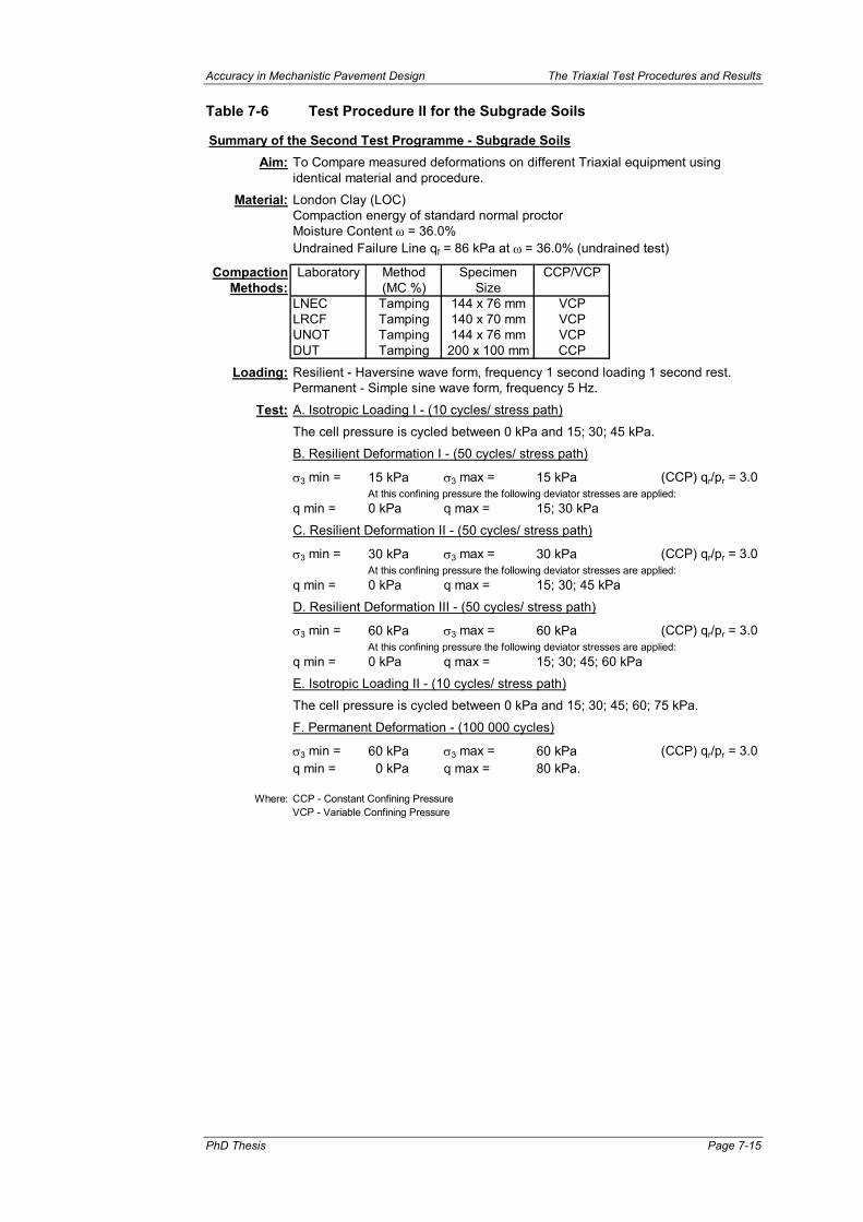
Accuracy in Mechanistic Pavement Design The Triaxial Test Procedures and Results
PhD Thesis Page 7-15
Table 7-6 Test Procedure II for the Subgrade Soils
Summary of the Second Test Programme - Subgrade SoilsAim: To Compare measured deformations on different Triaxial equipment using
identical material and procedure.
Material: London Clay (LOC)Compaction energy of standard normal proctorMoisture Content ω = 36.0%Undrained Failure Line qf = 86 kPa at ω = 36.0% (undrained test)
Compaction Laboratory Method Specimen CCP/VCPMethods: (MC %) Size
LNEC Tamping 144 x 76 mm VCPLRCF Tamping 140 x 70 mm VCPUNOT Tamping 144 x 76 mm VCPDUT Tamping 200 x 100 mm CCP
Loading: Resilient - Haversine wave form, frequency 1 second loading 1 second rest.Permanent - Simple sine wave form, frequency 5 Hz.
Test: A. Isotropic Loading I - (10 cycles/ stress path)
The cell pressure is cycled between 0 kPa and 15; 30; 45 kPa.
B. Resilient Deformation I - (50 cycles/ stress path)
σ3 min = 15 kPa σ3 max = 15 kPa (CCP) qr/pr = 3.0At this confining pressure the following deviator stresses are applied:
q min = 0 kPa q max = 15; 30 kPa
C. Resilient Deformation II - (50 cycles/ stress path)
σ3 min = 30 kPa σ3 max = 30 kPa (CCP) qr/pr = 3.0At this confining pressure the following deviator stresses are applied:
q min = 0 kPa q max = 15; 30; 45 kPa
D. Resilient Deformation III - (50 cycles/ stress path)
σ3 min = 60 kPa σ3 max = 60 kPa (CCP) qr/pr = 3.0At this confining pressure the following deviator stresses are applied:
q min = 0 kPa q max = 15; 30; 45; 60 kPa
E. Isotropic Loading II - (10 cycles/ stress path)
The cell pressure is cycled between 0 kPa and 15; 30; 45; 60; 75 kPa.
F. Permanent Deformation - (100 000 cycles)
σ3 min = 60 kPa σ3 max = 60 kPa (CCP) qr/pr = 3.0q min = 0 kPa q max = 80 kPa.
Where: CCP - Constant Confining PressureVCP - Variable Confining Pressure
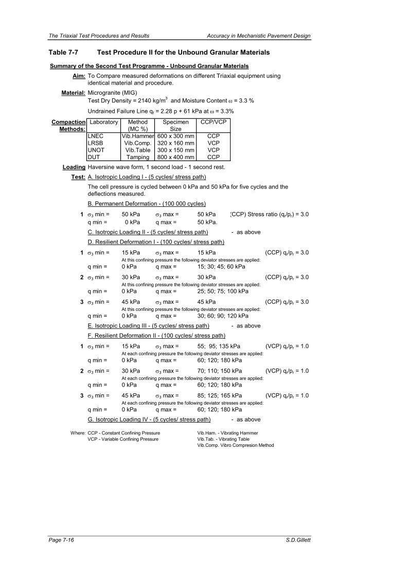
The Triaxial Test Procedures and Results Accuracy in Mechanistic Pavement Design
Page 7-16 S.D.Gillett
Table 7-7 Test Procedure II for the Unbound Granular Materials
Summary of the Second Test Programme - Unbound Granular MaterialsAim: To Compare measured deformations on different Triaxial equipment using
identical material and procedure.
Material: Microgranite (MIG)Test Dry Density = 2140 kg/m3 and Moisture Content ω = 3.3 %
Undrained Failure Line qf = 2.28 p + 61 kPa at ω = 3.3%
Compaction Laboratory Method Specimen CCP/VCPMethods: (MC %) Size
LNEC Vib.Hammer 600 x 300 mm CCPLRSB Vib.Comp. 320 x 160 mm VCPUNOT Vib.Table 300 x 150 mm VCPDUT Tamping 800 x 400 mm CCP
Loading Haversine wave form, 1 second load - 1 second rest.
Test: A. Isotropic Loading I - (5 cycles/ stress path)
The cell pressure is cycled between 0 kPa and 50 kPa for five cycles and thedeflections measured.
B. Permanent Deformation - (100 000 cycles)
1 σ3 min = 50 kPa σ3 max = 50 kPa (CCP) Stress ratio (qr/pr) = 3.0q min = 0 kPa q max = 50 kPa.
C. Isotropic Loading II - (5 cycles/ stress path) - as above
D. Resilient Deformation I - (100 cycles/ stress path)
1 σ3 min = 15 kPa σ3 max = 15 kPa (CCP) qr/pr = 3.0At this confining pressure the following deviator stresses are applied:
q min = 0 kPa q max = 15; 30; 45; 60 kPa
2 σ3 min = 30 kPa σ3 max = 30 kPa (CCP) qr/pr = 3.0At this confining pressure the following deviator stresses are applied:
q min = 0 kPa q max = 25; 50; 75; 100 kPa
3 σ3 min = 45 kPa σ3 max = 45 kPa (CCP) qr/pr = 3.0At this confining pressure the following deviator stresses are applied:
q min = 0 kPa q max = 30; 60; 90; 120 kPa
E. Isotropic Loading III - (5 cycles/ stress path) - as above
F. Resilient Deformation II - (100 cycles/ stress path)
1 σ3 min = 15 kPa σ3 max = 55; 95; 135 kPa (VCP) qr/pr = 1.0At each confining pressure the following deviator stresses are applied:
q min = 0 kPa q max = 60; 120; 180 kPa
2 σ3 min = 30 kPa σ3 max = 70; 110; 150 kPa (VCP) qr/pr = 1.0At each confining pressure the following deviator stresses are applied:
q min = 0 kPa q max = 60; 120; 180 kPa
3 σ3 min = 45 kPa σ3 max = 85; 125; 165 kPa (VCP) qr/pr = 1.0At each confining pressure the following deviator stresses are applied:
q min = 0 kPa q max = 60; 120; 180 kPa
G. Isotropic Loading IV - (5 cycles/ stress path) - as above
Where: CCP - Constant Confining Pressure Vib.Ham. - Vibrating HammerVCP - Variable Confining Pressure Vib.Tab. - Vibrating Table
Vib.Comp. Vibro Compresion Method

Accuracy in Mechanistic Pavement Design The Triaxial Test Procedures and Results
PhD Thesis Page 7-17
As a consequence of this more effort was made in obtaining specimens, at the various
laboratories, that were at the same densities and moisture condition. Some
investigation into the variation of results, as a function of the methods of compaction
of base material was conducted during this phase. The specified compaction
methods are shown in Table 7-8.
Table 7-8 Compaction Methods Specified
Method Laboratory Specimen Size
Vibrating Hammer LNEC 600 x 300 mm
Vibrating Compression Apparatus LRSB 320 x 160 mm
Vibrating Table UNOT 300 x 150 mm
Tamping DUT 800 x 400 mm
Each of the laboratories had developed various methods of specimen manufacture
and compaction and it was not possible to change this easily. The time and cost of
developing and constructing a new compaction apparatus was considered to be too
great. However, if a standard test procedure is to be formulated, consideration must
be given to a standard method of compaction, which is relatively easy, quick and
effective.
7.4.1 Permanent Strain Behaviour
The permanent strain on subgrade soils during conditioning was not measured. This
was because the conditioning is meant to simply bed the specimen against the
apparatus platens and to ensure that the instrumentation is functioning in order that
the specimens are ready for the resilient phase of the test rather than measure the
permanent deformation under loading. Once the resilient tests are completed then a
higher loading magnitude is applied to the specimens and the permanent deformation
measured.
The axial permanent strains measured on the unbound granular specimens by the
four laboratories were found to vary somewhat as is clearly shown in Figure 7-7. The
mean values range from 3.6 x 10⁻⁴ µε at LNEC to 37.0 x 10⁻⁴ µε at LRSB, as shown in
Table 7-9, a factor of approximately 10, which is an unacceptable difference. It was

The Triaxial Test Procedures and Results Accuracy in Mechanistic Pavement Design
Page 7-18 S.D.Gillett
concluded that this range is probably caused by differences in the compaction method
used by the laboratories. Methods of compaction which induce high levels of shear,
such as the vibrating hammer (LNEC) and manual tamping under cyclic preloading
(DUT) result in lower permanent strains than the methods where the compaction is full
face and tend not to induce such high levels of shear, such as the vibrocompression
apparatus (LRSB) and vibrating table and full face static load (UNOT).
Table 7-9 Comparison of the Permanent Axial Strain for Unbound Granular Specimens
Strain Values after Specimen Conditioning [20,000 cycles] at Various Laboratories (µε x 10-4) Tests Conducted LNEC UNOT LRSB DUT
Specimen 1 4.1 8.9 32.6 4.3
Specimen 2 1.3 29.9 38.6 3.9
Specimen 3 5.5 21.5 40.2 4.9
Specimen 4 3.5
Mean 3.6 20.1 37.1 4.4
Standard Deviation 1.7 10.6 4.0 0.5
Coefficient of Variation 49% 53% 11% 12%
The mean value, from the results of the four laboratories is, 16 µε, the standard
deviation is 16 µε. This is very poor since it is the same as the mean value, the
Coefficient of Variation is 97%, which, too is very poor. During these conditioning
tests, it was observed that the permanent strains measured per load cycle decreased
significantly from the start of the load applications but stabilised after approximately
5,000 cycles. This confirms the importance of applying a cyclic conditioning before
studying the resilient behaviour of a granular material.

The Triaxial Test Procedures and Results Accuracy in Mechanistic Pavement Design
PhD Thesis Page 7-19
Figure 7-7 Permanent Strains Measured in Different Apparatus while testing Microgranite
LNEC - UGM (TP2)
0123456789
10
0 5,000 10,000 15,000 20,000No.of Cycles (N)
Stra
in ( µ
ε x
10-4
)
UNOT - UGM (TP2)
0
5
10
15
20
25
30
35
0 5,000 10,000 15,000 20,000No.of Cycles (N)
Stra
in ( µ
ε x
10-4
)
LRSB - UGM (TP2)
0
5
10
15
20
25
30
35
40
45
0 5,000 10,000 15,000 20,000No.of Cycles (N)
Stra
in ( µ
ε x
10-4
)
DUT - UGM (TP2)
0
1
2
3
4
5
6
0 5,000 10,000 15,000 20,000No.of Cycles (N)
Stra
in ( µ
ε x
10-4
)

The Triaxial Test Procedures and Results Accuracy in Mechanistic Pavement Design
Page 7-20 S.D.Gillett
7.4.2 Resilient Strain Behaviour
Resilient tests were conducted on both granular base materials and subgrade soils at
each of the four laboratories. Again different behaviour was found from one laboratory
to another. The results, however, were better than those obtained during the earlier
Test Programme I. An example of the test results for varying deviator stress for the
subgrade soil and unbound granular material is shown in Figure 7-8 and Figure 7-9
respectively.
Unbound Granular Material
Resilient measurements, taken during the conditioning stage of the tests, on
specimens of unbound granular material were conducted for the stress path of
deviatoric stress cycled between 0 and 130 kPa with a constant confining pressure of
50 kPa. For the resilient axial strains, the agreement between the laboratories is
much improved as shown in Table 7-10. UNOT obtained somewhat higher and more
varied values, which was considered to be due to generally low and scattered dry
densities attained during the manufacture of the specimens.
Table 7-10 Comparison of the Resilient Axial Strain for Unbound Granular Specimens (TP2)
Resilient Axial Strain (µε) at p1 = 50 kPa; qr = 0 - 130 kPa Tests Conducted
LNEC UNOT LRSB DUT
Specimen 1 351 661 345 426
Specimen 2 309 568 378 350
Specimen 3 315 450 452 448
Specimen 4 392
Mean 342 460 392 408
Standard Deviation 38 106 55 51
Coefficient of Variation 11% 19% 14% 13%
The mean value from the four laboratories is 401 µε, the standard deviation is 49 µε
and the Coefficient of Variation is 12%, which is a considerable improvement on the
earlier test programme.

The Triaxial Test Procedures and Results Accuracy in Mechanistic Pavement Design
PhD Thesis Page 7-21
Figure 7-8 Resilient Strains Measured on Specimens of Subgrade Soil during Test Programme II
London Clay (LOC)
-8000
-6000
-4000
-2000
0
2000
4000
6000
8000
10000
12000
10 15 20 25 30 35 40 45 50Repeated Deviatior Stress [qr] (kPa)
Res
ilient
Stra
in ( µ
ε)
LNECUNOTLRCFDUT
Axial Strain
Radial Strain

The Triaxial Test Procedures and Results Accuracy in Mechanistic Pavement Design
S.D.Gillett Page 7-22
Figure 7-9 Resilient Strains Measured on Specimens of Unbound Granular Base during Test Programme II
Microgranite (MIG)
-300
-200
-100
0
100
200
300
400
500
600
20 30 40 50 60 70 80 90 100 110 120Repeated Deviatior Stress [qr] (kPa)
Res
ilient
Stra
in ( µ
ε) LNECUNOTLRSBDUT
Axial Strain
Radial Strain

Accuracy in Mechanistic Pavement Design The Triaxial Test Procedures and Results
PhD Thesis Page 7-23
The radial resilient strains shown in Table 7-11 are less satisfactory since there is a
large variation between the results, with UNOT being about 4 times greater than
LNEC.
Table 7-11 Comparison of the Resilient Radial Strain for Unbound Granular Specimens (TP2)
Resilient Radial Strain (µε) at p1 = 50 kPa; qr = 0 - 130 kPa Tests Conducted
LNEC UNOT LRSB DUT
Specimen 1 -77 -198 -97 -131
Specimen 2 -37 -254 -135 -169
Specimen 3 -38 -218 -176 -138
Specimen 4 -72
Mean -56 -223 -136 -146
Standard Deviation 21 28 40 20
Coefficient of Variation 38% 13% 29% 14%
The mean value from the four laboratories is -140 µε, the standard deviation is 68 µε
and the Coefficient of Variation is 49%, which is a great deal poorer than the 12% of
the axial resilient strain results above. It is thus surmised that there are greater errors
in the radial measurement systems than the axial measuring systems, something that
was shown during the earlier test programme as well.
For the resilient axial strains, relatively small differences were observed between the
mean values from the four laboratories but the coefficient of variation (repeatability)
was much greater. The best repeatability was obtained where large specimens were
used (LNEC and DUT). In addition the best repeatability was obtained where less
scattered dry densities were recorded (LNEC and LRSB), thus the method of
compaction is important.
For the radial strains and for the Poisson's ratio (which is largely dependent on radial
strains accuracy), the variation of the results was large at all the laboratories. These
poor results show that there are difficulties associated with the measurement of radial
strains in these triaxial tests. This can be explained by the fact that the radial strains
measured were particularly small, for the LRSB specimens, for example. This

The Triaxial Test Procedures and Results Accuracy in Mechanistic Pavement Design
Page 7-24 S.D.Gillett
corresponds to radial displacements lower than 16 µε, which is near the limit of the
capability of some instrumentation. Further, fixing of the radial instrumentation to the
specimen poses difficulties and is a probable source of errors. The compaction of the
material around the studs, which are embedded into the materials, or the effect of the
membrane when the instrumentation is glued on to the membrane could have caused
errors.
Subgrade Soils
Unfortunately, LNEC did not record the strains during the 100,000 cycle conditioning
phase. UNOT and DUT recorded permanent axial strains of similar magnitude during
the conditioning phase as shown in Table 7-12. LRCF recorded very small values,
about 60 times smaller than the other laboratories, indicating some error. Larger
differences were found between the mean values of the permanent radial strains
obtained by the three laboratories. The variation of results from a single laboratory
was found to be greater, with coefficients of variation of between 20 and 40%. Again,
LRPC recorded extremely small strains in comparison with the other laboratories.
Table 7-12 Comparison of the Permanent Strains for Subgrade Soil Specimens (TP2)
Strain Values after Specimen Conditioning [100,000 cycles] at Various Laboratories (µε x 10-4)
Axial Strain Radial Strain Tests Conducted
UNOT LRCF DUT UNOT LRCF DUT
Specimen 1 148 3.5 335 -31.5 -1.2 -212
Specimen 2 231 3.5 194 -105.0 -1.9 -109
Specimen 3 225 3.6 211 -85.3 -1.3 -138
Mean 201 3.5 247 -73.8 -1.5 -153
Standard Deviation 37.9 0.0 63.1 31.0 0.3 43.6
Coefficient of Variation 19% 1% 26% 42% 21% 29%
Table 7-13 and Table 7-14 show a comparison of the strains measured on the
specimens of subgrade soils conducted at the four different laboratories as part of
Phase 2. These results are for a fixed confining pressure of 30 kPa and varying
deviator stresses as shown.

Accuracy in Mechanistic Pavement Design The Triaxial Test Procedures and Results
PhD Thesis Page 7-25
Table 7-13 Comparison of the Axial Strains for London Clay Specimens (TP2)
Resilient Axial Strain (µε) at p1 = 30 kPa; qr = 0 - 45 kPa Tests Conducted
LNEC UNOT LRCF DUT
Mean 3136 3465 1514 5173
Standard Deviation 645 651 200 719
Coefficient of Variation 21% 19% 13% 14%
Table 7-14 Comparison of the Resilient Strains London Clay Specimens (TP2)
Resilient Radial Strain (µε) at p1 = 30 kPa; qr = 0 - 45 kPa Tests Conducted
LNEC UNOT LRCF DUT
Mean -2396 -2147 -1049 -2789
Standard Deviation 623 960 284 502
Coefficient of Variation 26% 45% 27% 18%
Two laboratories (LNEC and UNOT) obtained similar mean axial strain values. The
axial strain values measured at DUT were largest, which is to be expected, because
the axial strain is measured with a transducer placed outside the triaxial cell and this
tends to overestimate the strain {Lashine (1971), Parr (1972), Barksdale (1972b)}.
The reason why LRCF obtained results of approximately half those of LNEC and
UNOT is unclear.
Within a single laboratory, the smallest variation, or scatter of axial strain results, was
found at LRCF, with a coefficient of variation of 13%. Since this laboratory has
greater experience in this type of testing it is considered that both the operators and
the methods of testing were more competent than those at the other laboratories, who
has less experience in testing, and therefore the repeatability of tests was better. The
largest scatter was observed at LNEC. This is thought to be due to the fact that this
laboratory was still developing their apparatus and test procedures so that greater
operator errors were likely to occur.

The Triaxial Test Procedures and Results Accuracy in Mechanistic Pavement Design
Page 7-26 S.D.Gillett
For resilient radial strains, as shown in Table 7-14, it was noted that LNEC, UNOT and
DUT all used proximity transducers for measuring radial strains and obtaining mean
radial strain values of fair agreement. LRCF, however, obtained systematically about
2 times smaller values of radial strain than the other laboratories.
The scatter of the radial strain results is larger than those found for axial strains. DUT
had the lowest variation, which might be due to their using larger specimens (100 mm
in diameter) than the other laboratories. The poorest variation was found at UNOT,
with coefficients of variation exceeding 40 %.
The resilient modulus has been calculated for each of the different deviator stress
applications and the non-linearity is clear as shown in Table 7-15. These results
generally follow the trend of the strains, except that the differences between the
laboratories seem smaller, for example 33; 31 and 29 MPa obtained for resilient
modulus at qr = 15 kPa.
Table 7-15 Comparison of the Resilient Modulus for Subgrade Soil Specimens (TP2)
Resilient Modulus (MPa) at p1 = 30 kPa Tests
Conducted LNEC UNOT LRCF DUT
Deviator Stress (kPa) 0-15 0-30 0-45 0-15 0-30 0-45 0-15 0-30 0-45 0-15 0-30 0-45
Mean 33 25 14 31 21 14 65 49 30 29 15 9
Standard Deviation 8.5 7.5 2.1 7.1 4.3 3.0 2.1 4.2 4.4 5.9 2.2 1.0
Coefficient of Variation (%)
26 30 15 23 21 22 3 9 15 21 15 12
After assessing the results of Phase 1 the test procedure was modified and a series of
tests was conducted by each of the four laboratories on similar materials (Phase 2
and again somewhat different results in measured strains were obtained. It was thus
decided to exclude all possible influences related to natural materials and specimen
manufacturing differences and to test an artificial specimen (Phase 3). All of the
results for this test programme (Phase 2) are contained in Appendix F.2.

Accuracy in Mechanistic Pavement Design The Triaxial Test Procedures and Results
PhD Thesis Page 7-27
7.5 PHASE 3 - ROUND ROBIN TESTING ON THE ARTIFICIAL SPECIMEN
The material used for these tests was Polytetrafluoroethylene (PTFE), as described in
the previous chapter. In order to eliminate the time dependent specimen response,
under loading, the generated loading signal was applied as a static square signal as
shown in Table 7-16.
Table 7-16 Loading Regime Applied to the Artificial Specimen
Test No. Time (sec)
Confining Pressure σ3 (kPa)
Deviator Stress q (kPa)
0 - 3600 250 0 1
3600 - 7200 0 0
0 - 3600 250 375 2
3600 - 7200 0 0
0 - 3600 100 600 3
3600 - 7200 0 0
As the laboratories had equipment of different dimensions, the artificial specimen was
progressively reduced in size, as it was tested in smaller capacity apparatus. Thus, it
may be argued, there was some difference between the specimens as assessed at
the different laboratories. Nevertheless, this difference is believed to be small when
compared with that inherent in unbound granular materials and soils. A limitation on
the initial size of the artificial specimen meant that it was not possible to include the
large DUT and LNEC apparatuses in the comparisons. The tests were conducted in
laboratories as listed in Table 7-17. This table also shows the specimen size (thus
identifies the actual apparatus) and the temperature at which the test was conducted.
The instruments were affixed to the artificial specimen with, as near as possible, the
same methods as for the real specimens. The principal limitation was that studs/
vanes could not be embedded, so the external elements of the fixing were screwed
into holes tapped in the specimen. It is anticipated that this would have introduced
some improvement in performance over that recorded with real specimens.

The Triaxial Test Procedures and Results Accuracy in Mechanistic Pavement Design
Page 7-28 S.D.Gillett
Table 7-17 The Apparatus and the Corresponding Specimen Size
Apparatus Specimen Size [Height x Diameter] (mm)
Temperature (°C)
LRSB 320 x 160 18
UNOT1 320 x 160 24
DUT1 210 x 102 22
LNEC 144 x 76 21
UNOT2 144 x 76 24
LRCF2 140 x 70 18 Notes: 1. Small static deviator stress (6 kPa) constantly applied. 2. Stress levels applied are lower than stipulated.
Applied Loads (Stress)
There was some variation in the applied load from that stipulated as shown in Table
7-18, which shows the recorded stresses. The stresses applied to the specimen at
LRCF were much lower than those stipulated, this being due to deficiencies in their
apparatus. Consequently these results are not included in the arithmetic means. With
the exception of the LRCF loading the applied loading was very uniform with
coefficients of variation of less than 1%.
Table 7-18 Recorded Stresses Applied to the Artificial Specimen
Test 1 Test 2 Test 3 Apparatus σ1r
(kPa) σ3r
(kPa) σ1r
(kPa) σ3r
(kPa) σ1r
(kPa) σ3r
(kPa)
LNEC 250 250 643 249 710 98
UNOT1 248 248 618 246 701 100
UNOT2 250 250 625 250 700 100
LRSB 250 250 625 250 700 100
LRCF 236 236 326 237 176 87
DUT 250 250 626 250 686 100
Mean 250 250 627 249 699 100
Standard Deviation 1 1 9 2 9 1
Coefficient of Variation 0% 0% 1% 1% 1% 1%

Accuracy in Mechanistic Pavement Design The Triaxial Test Procedures and Results
PhD Thesis Page 7-29
Test 1 – Deformation (Strain) Measurement
The deformations measured on the specimens under this isotropic loading were very
small, as is shown in Figure 7-10, due to small loading stresses. This test illustrates
that the accuracy of the systems are limited. During these low stress levels the
instrumentation was found to wander and since the strains were very small the
wandering might have exceeded the actual strain. This is clearly demonstrated by the
LNEC Axial data in Figure 7-10, which ‘jumps’ in multiples of 25 µε.
Figure 7-10 Artificial Specimen Test 1
Test 1 - Axial Strain Measurement
-250
-200
-150
-100
-50
0
50
100
150
0 1,000 2,000 3,000 4,000 5,000 6,000 7,000 8,000Time (sec)
Axi
al S
train
( µε)
LNEC 144x76 mmUNOT1 300x150 mmUNOT2 144x70 mmLRSB 320x160 mmLRCF 140x70 mmDUT 144x76 mm
Test 1 - Radial Strain Measurement
-400
-200
0
200
400
600
800
0 1,000 2,000 3,000 4,000 5,000 6,000 7,000 8,000Time (sec)
Rad
ial S
train
( µε)

The Triaxial Test Procedures and Results Accuracy in Mechanistic Pavement Design
Page 7-30 S.D.Gillett
Thus there is an obvious error associated with the minimum reading that the
instrumentation can measure. In general the instrumentation systems are only able to
measure strains of greater than about 60 µε as shown in Table 7-19.
The radial strain measurements made by LNEC and UNOT2 are much higher that
those of the other instruments. These apparatus are similar (both developed at
Nottingham) and both use proximity transducers to measure the radial strain. The
remaining instruments show similar magnitudes of strain measurement.
Complete results of the tests conducted during this experiment are contained in
Appendix E.
Table 7-19 The Average and Minimum Instrumentation Wandering
Axial Strain (µε) Radial Strain (µε) Apparatus
Average Minimum Average Minimum
LNEC 25 25 22 4
UNOT1 9 8 26 4
UNOT2 36 3 60 12
LRSB 29 10 50 13
LRCF 3 2 3 1
DUT 20 1 16 1
Test 2 and Test 3 – Deformation (Strain) Measurement
Axial loading applied to the specimen in these two tests resulted in much larger strains
being recorded. As shown in Figure 7-11 and Figure 7-12he axial load imposed by
LRCF was considerably lower than that applied by the other laboratories, thus the
strains are expected to be much less as is the case. UNOT yielded a much larger
axial strain for their small apparatus and a lower axial strain for their large apparatus.
Generally all of the radial strains coincide well. Again, however, some variation is
seen in the UNOT results. The trends are the same for Test 2 and Test 3 for both the
axial and radial strains. Table 7-20 contains a summary of the strains for each of the
apparatus during these tests. The deviation from the arithmetic mean is shown in this
table as a percentage in each case. These figures show that the deviation is quite
large, as expected for LRCF, but also for UNOT.

Accuracy in Mechanistic Pavement Design The Triaxial Test Procedures and Results
PhD Thesis Page 7-31
Figure 7-11 Artificial Specimen Test 2
Test 2 - Axial Strain Measurement
0
2,000
4,000
6,000
8,000
10,000
12,000
0 1,000 2,000 3,000 4,000 5,000 6,000 7,000 8,000Time (sec)
Axi
al S
train
(me)
LNEC 144x76 mmUNOT1 300x150 mmUNOT2 144x70 mmLRSB 320x160 mmLRCF 140x70 mmDUT 144x76 mm
Test 2 - Radial Strain Measurement
-4,500
-4,000
-3,500
-3,000
-2,500
-2,000
-1,500
-1,000
-500
0
0 1,000 2,000 3,000 4,000 5,000 6,000 7,000 8,000Time (sec)
Rad
ial S
train
( µε)

The Triaxial Test Procedures and Results Accuracy in Mechanistic Pavement Design
Page 7-32 S.D.Gillett
Figure 7-12 Artificial Specimen Test 3
Test 3 - Axial Strain Measurement
0
2,000
4,000
6,000
8,000
10,000
12,000
14,000
16,000
18,000
0 1,000 2,000 3,000 4,000 5,000 6,000 7,000 8,000Time (sec)
Axi
al S
train
( µε)
LNEC 144x76 mmUNOT1 300x150 mmUNOT2 144x70 mmLRSB 320x160 mmLRCF 140x70 mmDUT 144x76 mm
Test 3 - Radial Strain Measurement
-7,000
-6,000
-5,000
-4,000
-3,000
-2,000
-1,000
0
0 1,000 2,000 3,000 4,000 5,000 6,000 7,000 8,000Time (sec)
Rad
ial S
train
( µε)

Accuracy in Mechanistic Pavement Design The Triaxial Test Procedures and Results
PhD Thesis Page 7-33
Table 7-20 Recorded Strains on the Artificial Specimen
Test 2 Test 3
Axial Radial Axial Radial Laboratory
(µε) d (µε) d (µε) d (µε) d
LNEC 7081 6% -3431 1% 10710 7% -5756 0%
UNOT1 5357 29% -3215 7% 9320 19% -5296 8%
UNOT2 10978 46% -3796 9% 14858 29% -6049 5%
LRSB 7130 5% -3463 0% 11640 1% -5725 0%
LRCF 5252 30% -803 77% 5280 54% -1180 79%
DUT 7074 6% -3440 1% 10992 4% -5908 3%
Mean 7524 -3469 11504 -5747
Standard Deviation 2072 208 2057 283
Coefficient of Variation 28% 6% 18% 5%
Notes: 1. Mean, Standard Deviation and Coefficient of Variation exclude LRCF value. 2. d – Deviation from the Mean for a single value.
During the two earlier test phases, where tests were conducted on actual road
construction material, it was concluded that the radial measurements were less
accurate than the axial measurements. However, during this test phase this is clearly
contradicted. It is therefore concluded that the inaccuracies in radial measurement
when testing road construction materials is due to the specimens rather than the
instrumentation. The possible causes for these inaccuracies are:
• Specimen manufacture differences, for example single layer or multi-layer
• Methods of compaction, vibration or tamping and full-face or smaller;
• The methods of fixing the instrumentation to the specimens.
A further conclusion for this is that the axial displacement measurement is more
accurate with higher loads whereas the radial measurement was not affected by load
magnitude.
Resilient Modulus and Poisson’s Ratio
In order that the variations in the stress could be considered as a function of the
variations in the strain the resilient modulus and the Poisson’s ratio were calculated as

The Triaxial Test Procedures and Results Accuracy in Mechanistic Pavement Design
Page 7-34 S.D.Gillett
shown in Table 7-21. These material parameters or characteristics were calculated at
a particular stress value, based on the standard used at LRSB, of pr = 250 kPa and
qr/pr = 2. Again, the LRCF values were low, as shown by the deviation from the mean,
and thus have been excluded from the mean, standard deviation and coefficient of
variation.
Table 7-21 Resilient Moduli and Poison's Ratio for the Artificial Specimen
Test 2 Test 3 Apparatus
Mr d ν d Mr d ν d
LNEC 71 4% 0.49 0% 64 7% 0.53 4%
UNOT1 89 31% 0.53 8% 72 21% 0.54 8%
UNOT2 44 35% 0.44 10% 45 24% 0.44 14%
LRSB 68 1% 0.50 1% 58 3% 0.49 2%
LRCF 24 65% 0.45 8% 22 63% 0.42 17%
DUT 68 0% 0.50 1% 60 0% 0.52 4%
Mean 68 0.49 60 0.51
Standard Deviation 16 0.03 10 0.04
Coefficient of Variation 24% 6% 16% 8%
Notes: 1. Mean, Standard Deviation and Coefficient of Variation exclude LRCF data. 2. d – Deviation of the particular value from the mean 3. Mr – Resilient Modulus (MPa). 4. ν - Poisson’s Ratio
The Poisson’s ratio for this material is expected to be 0.5 and the results confirm this.
The coefficient of variation for the Poisson’s ratio is better than that for the resilient
modulus, since Poisson’s ratio is more dependent on the radial strain measurements,
which were found to have a lower variation than the axial strains. This too is to be
expected. The variation for resilient modulus is better for higher stresses, again
confirming the conclusions above.
7.6 PHASE 5 - THE PRINCIPAL TEST PROGRAMME
The principal test programme (Test Programme III) was established in order to
determine the behaviour of typical soils and unbound granular materials representing
those used in foundations of pavements and in the base layers of flexible pavements

Accuracy in Mechanistic Pavement Design The Triaxial Test Procedures and Results
PhD Thesis Page 7-35
respectively in Europe. Based on the findings of the three earlier test phases,
discussed above, the two test procedures were compiled. Details of the test
procedure are contained in Appendix D.3 and are summarised in Table 7-22 and
Table 7-23.
The third test programme was conducted at two laboratories (LRSB and LNEC) on
two unbound granular materials and two subgrade materials as discussed in the
procedure. The objective of this Phase was to collect meaningful data about typical
road construction materials found in Europe. The results from these tests, which
characterise typical road construction materials, are used in the mechanistic analysis
of typical pavement structures in the Chapter 9. All of the results for this test
programme (Phase 5) are contained in Appendix F.3.
7.7 COMPARISON OF METHODS SPECIMEN MANUFACTURE
Due to the conclusion that the different specimens are producing different recorded
strains depending on the method of manufacture a comparison of these compaction
methods is discussed here.
7.7.1 Subgrade Soils
Due to the fine grained nature of the clayey materials that comprise subgrade soils the
specimens can be relatively small, less than 100 mm diameter, and therefore these
specimens are much more easily handled than the larger granular base specimens.
During this work the tamping method of compaction was found to achieve the
specified densities at the required moisture contents. However, since particular
specimen densities were required for specified moisture contents it was often
necessary to vary the compactive effort experimentally until the correct density was
achieved. At LNEC an apparatus was used to confirm that the density was consistent
throughout the specimen. A nuclear density meter measured the relative density of
the specimen as it was spiralled slowly down past the point of measurement {Gomes
Correia (1985)}; this apparatus is shown in Photograph 7-1.
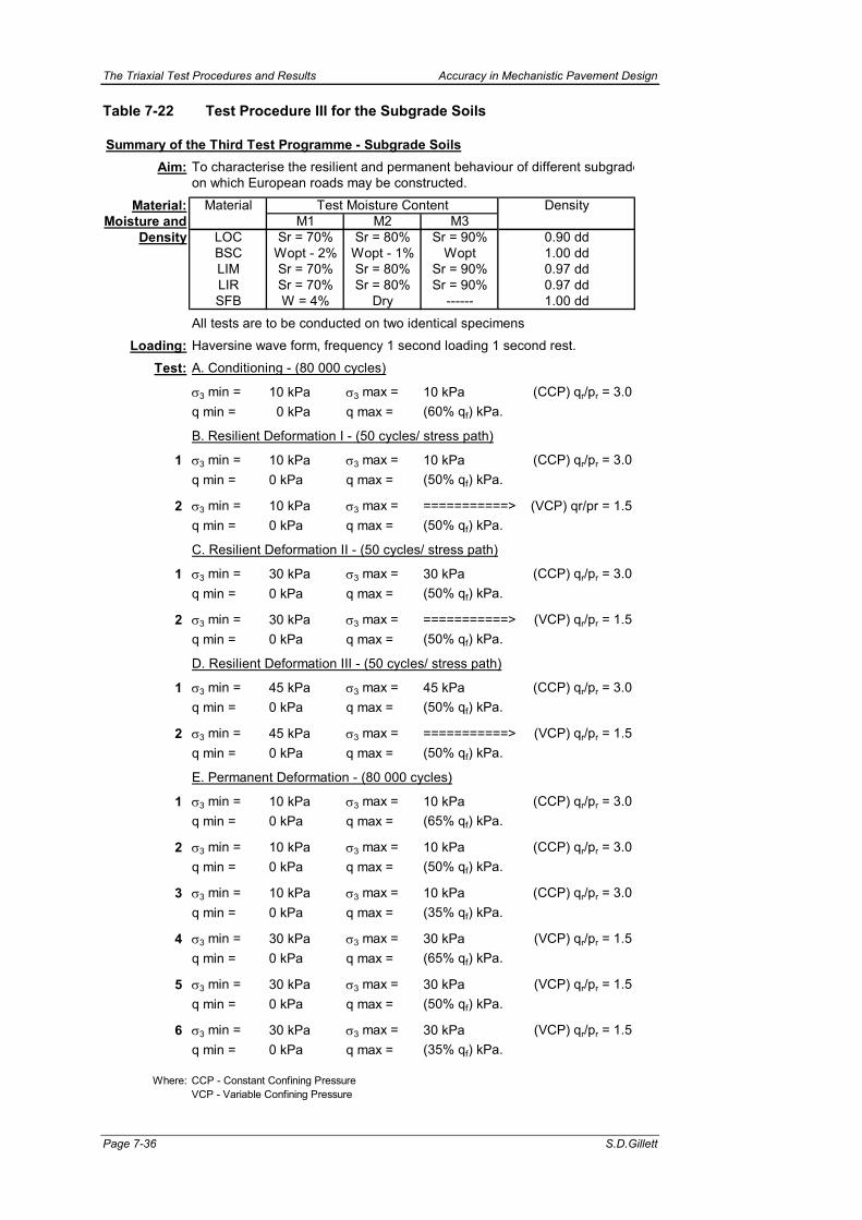
The Triaxial Test Procedures and Results Accuracy in Mechanistic Pavement Design
Page 7-36 S.D.Gillett
Table 7-22 Test Procedure III for the Subgrade Soils
Summary of the Third Test Programme - Subgrade SoilsAim: To characterise the resilient and permanent behaviour of different subgrade
on which European roads may be constructed.
Material: Material Test Moisture ContentMoisture and M1 M2 M3
Density LOC Sr = 70% Sr = 80% Sr = 90%BSC Wopt - 2% Wopt - 1% WoptLIM Sr = 70% Sr = 80% Sr = 90%LIR Sr = 70% Sr = 80% Sr = 90%SFB W = 4% Dry ------
All tests are to be conducted on two identical specimens
Loading: Haversine wave form, frequency 1 second loading 1 second rest.
Test: A. Conditioning - (80 000 cycles)
σ3 min = 10 kPa σ3 max = 10 kPa (CCP) qr/pr = 3.0q min = 0 kPa q max = (60% qf) kPa.
B. Resilient Deformation I - (50 cycles/ stress path)
1 σ3 min = 10 kPa σ3 max = 10 kPa (CCP) qr/pr = 3.0q min = 0 kPa q max = (50% qf) kPa.
2 σ3 min = 10 kPa σ3 max = ===========> (VCP) qr/pr = 1.5q min = 0 kPa q max = (50% qf) kPa.
C. Resilient Deformation II - (50 cycles/ stress path)
1 σ3 min = 30 kPa σ3 max = 30 kPa (CCP) qr/pr = 3.0q min = 0 kPa q max = (50% qf) kPa.
2 σ3 min = 30 kPa σ3 max = ===========> (VCP) qr/pr = 1.5q min = 0 kPa q max = (50% qf) kPa.
D. Resilient Deformation III - (50 cycles/ stress path)
1 σ3 min = 45 kPa σ3 max = 45 kPa (CCP) qr/pr = 3.0q min = 0 kPa q max = (50% qf) kPa.
2 σ3 min = 45 kPa σ3 max = ===========> (VCP) qr/pr = 1.5q min = 0 kPa q max = (50% qf) kPa.
E. Permanent Deformation - (80 000 cycles)
1 σ3 min = 10 kPa σ3 max = 10 kPa (CCP) qr/pr = 3.0q min = 0 kPa q max = (65% qf) kPa.
2 σ3 min = 10 kPa σ3 max = 10 kPa (CCP) qr/pr = 3.0q min = 0 kPa q max = (50% qf) kPa.
3 σ3 min = 10 kPa σ3 max = 10 kPa (CCP) qr/pr = 3.0q min = 0 kPa q max = (35% qf) kPa.
4 σ3 min = 30 kPa σ3 max = 30 kPa (VCP) qr/pr = 1.5q min = 0 kPa q max = (65% qf) kPa.
5 σ3 min = 30 kPa σ3 max = 30 kPa (VCP) qr/pr = 1.5q min = 0 kPa q max = (50% qf) kPa.
6 σ3 min = 30 kPa σ3 max = 30 kPa (VCP) qr/pr = 1.5q min = 0 kPa q max = (35% qf) kPa.
Where: CCP - Constant Confining PressureVCP - Variable Confining Pressure
0.97 dd0.97 dd1.00 dd
Density
0.90 dd1.00 dd
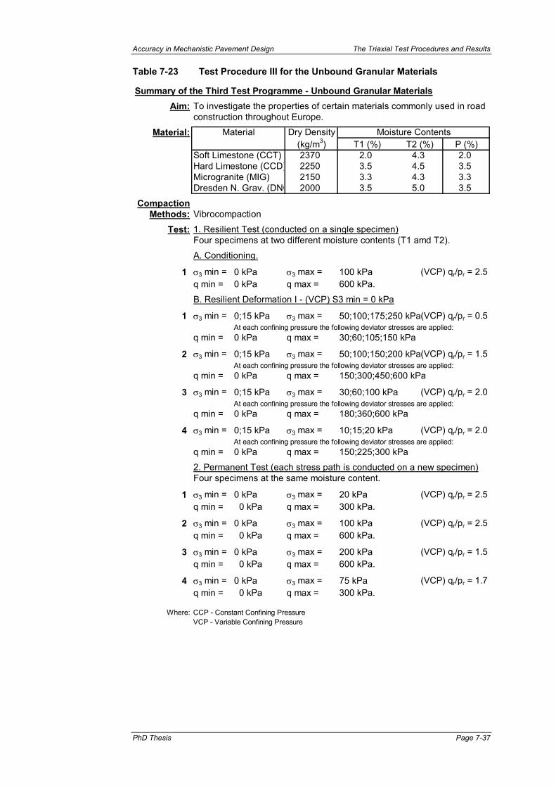
Accuracy in Mechanistic Pavement Design The Triaxial Test Procedures and Results
PhD Thesis Page 7-37
Table 7-23 Test Procedure III for the Unbound Granular Materials
Summary of the Third Test Programme - Unbound Granular MaterialsAim: To investigate the properties of certain materials commonly used in road
construction throughout Europe.
Material: Material Dry Density Moisture Contents(kg/m3) T1 (%) T2 (%) P (%)
Soft Limestone (CCT) 2370 2.0 4.3 2.0Hard Limestone (CCD) 2250 3.5 4.5 3.5Microgranite (MIG) 2150 3.3 4.3 3.3Dresden N. Grav. (DNG 2000 3.5 5.0 3.5
CompactionMethods: Vibrocompaction
Test: 1. Resilient Test (conducted on a single specimen)Four specimens at two different moisture contents (T1 amd T2).
A. Conditioning.
1 σ3 min = 0 kPa σ3 max = 100 kPa (VCP) qr/pr = 2.5q min = 0 kPa q max = 600 kPa.
B. Resilient Deformation I - (VCP) S3 min = 0 kPa
1 σ3 min = 0;15 kPa σ3 max = 50;100;175;250 kPa(VCP) qr/pr = 0.5At each confining pressure the following deviator stresses are applied:
q min = 0 kPa q max = 30;60;105;150 kPa
2 σ3 min = 0;15 kPa σ3 max = 50;100;150;200 kPa(VCP) qr/pr = 1.5At each confining pressure the following deviator stresses are applied:
q min = 0 kPa q max = 150;300;450;600 kPa
3 σ3 min = 0;15 kPa σ3 max = 30;60;100 kPa (VCP) qr/pr = 2.0At each confining pressure the following deviator stresses are applied:
q min = 0 kPa q max = 180;360;600 kPa
4 σ3 min = 0;15 kPa σ3 max = 10;15;20 kPa (VCP) qr/pr = 2.0At each confining pressure the following deviator stresses are applied:
q min = 0 kPa q max = 150;225;300 kPa
2. Permanent Test (each stress path is conducted on a new specimen)Four specimens at the same moisture content.
1 σ3 min = 0 kPa σ3 max = 20 kPa (VCP) qr/pr = 2.5q min = 0 kPa q max = 300 kPa.
2 σ3 min = 0 kPa σ3 max = 100 kPa (VCP) qr/pr = 2.5q min = 0 kPa q max = 600 kPa.
3 σ3 min = 0 kPa σ3 max = 200 kPa (VCP) qr/pr = 1.5q min = 0 kPa q max = 600 kPa.
4 σ3 min = 0 kPa σ3 max = 75 kPa (VCP) qr/pr = 1.7q min = 0 kPa q max = 300 kPa.
Where: CCP - Constant Confining PressureVCP - Variable Confining Pressure

The Triaxial Test Procedures and Results Accuracy in Mechanistic Pavement Design
Page 7-38 S.D.Gillett
Photograph 7-1 Specimen Density Measurement at LNEC
Once compacted the strain measurement instrumentation can be successfully
attached to the specimen by using the cruciform vanes, described earlier, which are
easily pressed into the specimen. Due to the soft nature of these specimens,
however, a frame is used to support the instrumentation in order that it does not ‘hang’
on the specimens causing deformation.
7.7.2 Unbound Granular Materials
The compaction of granular materials is more complex due to the less cohesive nature
of the materials. Instrumentation cannot be pressed into the specimen and must
therefore be either ‘cast’ into the specimen during compaction or fixed to the specimen
after manufacture. During this project specimens were manufactured in multi-layers
using both tamping and vibrating hammers. It was found that specimens
manufactured by the tamping method were often not dense enough. The vibrating
hammer method gives better density due to shear forces applied. At UNOT
specimens were compacted using a vibrating table and a surcharge applied to the
material. The material was placed in the mould in five layers and compressed. At

Accuracy in Mechanistic Pavement Design The Triaxial Test Procedures and Results
PhD Thesis Page 7-39
LRSB, however, a specifically manufactured apparatus compacted the specimen in a
single layer to a particular density, thus eliminating the iterative method of attaining
the correct density for particular moisture contents. However, when the material is
compacted in a single layer there are some questions about the uniformity of the
density of the material throughout the specimen. LRSB checked this using a nuclear
device similar to that at LNEC described above. Both UNOT and LRSB use a full-face
plate with their vibrating methods, whereas at LNEC a smaller diameter plate was
used to compact up to eight layers. This method induces more shear into the material
and therefore greater densities are possible.
When the instrumentation studs are fixed to the mould, as is necessary for unbound
granular material, in order that they are embedded in the specimen, the studs inhibit
the compaction of the material directly around the studs. If the material is compacted
in layers the material can be specifically compacted around the studs. When the
material was compacted in a single layer substantial voids were found around the
studs. At LRSB these voids were filled with a cement mortar that fixed the studs in
position.
7.8 SUMMARY
After assessing the results of Phase 1 the test procedure was modified and a series of
tests were conducted by each of the four laboratories on similar materials (Phase 2).
Again different results in measured strain were obtained and it was decided to exclude
all possible influences related with testing of natural materials and to test an artificial
specimen (Phase 3). This was followed by the final phase, in which different materials
were tested in different laboratories in accordance to a common procedure, in order to
determine the characteristics of common road construction materials in Europe
(Phase 5). This extensive test programme has yielded sufficient data to enable a
detailed analysis of the results using mathematical models that attempt to describe the
behaviour of the materials under traffic loading conditions.
The Triaxial Test Procedures and Results Accuracy in Mechanistic Pavement Design
Page 7-40 S.D.Gillett
In order to obtain repeatable results a well-prescribed test procedure is necessary.
The test procedure should be as simple as possible removing all unnecessary actions
that might introduce operator peculiarities.
A reliable compaction method, producing homogeneous densities, is needed for the
preparation of the specimens. It was found that the magnitude of the permanent
strain (axial and radial) that occurred during the conditioning was dependent on the
method of compaction of the specimen, thus there is a need for a standardised
compaction method for triaxial specimens. The vibrocompression method used at
LRSB, for example, is fast (1 minute to compact a specimen), largely automated
(which reduces the operator's influence), and produces very homogeneous
specimens in density because the compaction is performed in one layer. For the
compaction of fine-grained materials often the simple method of tamping multiple
layers is used.
In summary it is clear that not only is there a large variation in the strains from
specimens tested in a single laboratory but the tests on the artificial specimen show
that there is also some discrepancy between laboratories. It is also apparent that
there is a substantial variation in the loads (stresses) applied to the specimens that
will have an obvious effect on the strains. It is, therefore, necessary to take this
difference in stress into consideration when comparing results.
However, large differences in the results are thought to be due to differences in the
compaction method used by the laboratories. Methods of compaction which induce
high levels of shear, such as the vibrating hammer (LNEC) and manual tamping under
cyclic preloading (DUT) result in lower permanent strains than the methods where the
compaction is full face and tend not to induce such high levels of shear, such as the
vibrocompression apparatus (LRSB) and vibrating table and full face static load
(UNOT).
The mean radial measurement for three specimens each manufactured and tested at
the four laboratories is -140 µε, the standard deviation is 68 µε and the Coefficient of
Variation is 49%, which is a great deal poorer than the 12% for the axial resilient strain

Accuracy in Mechanistic Pavement Design The Triaxial Test Procedures and Results
PhD Thesis Page 7-41
measured between the laboratories. It is thus surmised that there are greater errors
in the radial measurement systems than the axial measuring systems, substantiating
that found during the earlier test programme.
Larger specimens give less variable results, however large specimens require more
material, are more time consuming to fabricate, more difficult to manoeuvre and the
apparatus required to test them is much larger thus more expensive. Another
disadvantage of very large specimens is that they generally are not suitable for
performing variable confining pressure tests since they use internal vacuums.
For the unbound granular material the axial resilient strain results show little
systematic difference although improved readings appear to result from larger
specimen size. The variability in readings is particularly high for the UNOT tests
(which may be due to stud rotation generating apparent strain - sometimes increasing,
sometimes decreasing the measured values above the average obtained at all the
laboratories). For radial resilient strains all laboratories yielded a large scatter in
strain values. There was no systematic variation in radial strains between
laboratories.
Experiments with various on-sample instruments for measuring the axial and radial
strain of soil and aggregate specimens subjected to repeated load triaxial testing (at
different sizes at different laboratories) have been described. Results frequently differ,
but the origin of these differences is often unclear. After the completion of the test
programme on the artificial test programme some calibration of the various apparatus
and instrumentation was conducted and each laboratory's apparatus was harmonised
for the main test programme (Phase 5).
A number of methods of analysis will be tested and recommendations made as to how
this type of data should be analysed and what the expected errors due to test
apparatus and instrumentation and sample manufacture are. The significance of
these errors will be tested in a mechanistic pavement design method and
recommendations made.


Accuracy in Mechanistic Pavement Design Analysis and Modelling
PhD Thesis Page 8-1
8 ANALYSIS OF THE BEHAVIOUR OF THE MATERIALS BY ANALYTICAL MODELLING
8.1 INTRODUCTION
In chapter 5 the models that are to be used to describe the behaviour of the road
construction materials were discussed. During this chapter the results of the tests
from the three test phases, Phase 1, 2 and 5, are analysed and the results discussed.
Briefly, as stated in Chapter 5, the models chosen are as follows:
Models for all Road Construction Materials
a. Simple Linear Elastic Model
b. The k-theta model
c. The Uzan Model
For Fine Grained Subgrade Soils used in Road Construction
d. The Brown Model
e. The Loach model
For Unbound Granular Materials used in Road Construction
f. The Boyce model
g. The Mayhew model
8.2 DATA VERIFICATION AND MANIPULATION
After conducting the test and ‘capturing’ the data (stresses and strains) by some
method, it is necessary to appraise the data and to undertake data verification. The
data verification should exclude any erroneous results. Care, however, must be taken
that true results are not excluded, even if they appear erroneous. For example, as
has been shown, erroneous data occur as a result of small stress applications and
thus small strain measurements and these should be excluded from any modelling,
since they will effect the overall characterisation of the material.
A problem with data verification is that is it somewhat subjective. It is with this in mind
that a method was devised for this work, as described below.

Analysis and Modelling Accuracy in Mechanistic Pavement Design
Page 8-2 S.D.Gillett
8.2.1 Initial Screening (Removal of Obviously Poor Data)
The test results, as presented in the previous chapter, comprise spreadsheets
containing the stresses and strains for each stress path applied for each specimen
tested. The resilient modulus and the Poisson’s ratio are calculated for each stress
path. An initial screening pass is made that eliminates all data from any particular
stress path that does not comply with the following criteria:
• Poisson’ ratio 0 < ν < 1
• Experimental resilient modulus Mr > 0
• Repeated deviator stress qr > 0
• Final mean normal stress p2 > 0
Strictly speaking all materials should have a Poisson’s ratio of between 0 and 0.5.
This is because any material with a Poisson’s ratio of less than 0 would be collapsing
within itself, which would be clearly impossible for a compacted material. Some
dilation is, however, possible due to particles ‘rolling’ over one another therefore the
maximum Poisson’s ratio is taken to be 1. It is impossible for a material to have a
negative resilient modulus. The deviator stress can be negative when in-situ, but this
should not occur for conventional compressive triaxial testing. Similarly, the maximum
mean normal stress will always be positive for triaxial conditions.
The coefficients of the constitutive relationships (models) are calculated from the
results of the test data using the analytical methods described in this chapter. Once
the model coefficients have been established it is possible to calculate a predicted
resilient modulus value for each stress path, and for each relationship, and plot these
against the experimental values calculated for the particular stress path. An example
of this is shown graphically in Figure 8-1 for an unbound granular material and in
Figure 8-2 for a subgrade soil.

Accuracy in Mechanistic Pavement Design Analysis and Modelling
PhD Thesis Page 8-3
Figure 8-1 Comparison of the Experimental and Modelled Resilient Modulus for an Unbound Granular Material
Resilient Modulus of a Sample of Soft Limestone
0
300
600
900
1,200
0 300 600 900 1,200Experimental [Mre] (MPa)
Mod
elle
d [M
r] (M
Pa)
k-theta Uzan Boyce Mayhew
Figure 8-2 Comparison of the Experimental and Modelled Resilient Modulus for a Subgrade Soil
Resilient Modulus of a Sample of Siene et Marne Silt
100
150
200
250
300
100 150 200 250 300Experimental [Mre] (MPa)
Mod
elle
d [M
r] (M
Pa)
k-theta Uzan Brow n Loach
8.2.2 Secondary Screening (Removal of Outliers by Percentile)
The data is then screened to exclude the data from all stress paths that are outside
certain variations from the average. These values are termed as outliers. For this
study outliers are defined as those values outside the 95th percentile (95%’ile) of the

Analysis and Modelling Accuracy in Mechanistic Pavement Design
Page 8-4 S.D.Gillett
average (across all relevant models) of the absolute difference between the
experimental and modelled values for resilient modulus, shown by the equation:
[ ]MrMrAverageile 95%Outlier e −≥ Eqn.8-1
Where MrMre − is the absolute difference of the experimental and the modelled Resilient Modulus.
There are instances where a particular stress path is considered to be an outlier when
analysed by one particular model and not by the others. It is for this reason that the
average is used and the ‘erroneous’ data is excluded for all models. Therefore the
data is always exactly the same when applied to the different models for each
analytical sequence in the removal of outliers.
Once the outliers have been removed from the data, the parameters for each model
are calculated again and the modelled resilient modulus recalculated from this data.
This procedure of identifying outliers can be reapplied to the new data and so on. If a
vast sample size (which is normally distributed) were used then it would be expected
that one could continue to remove 5% of the worst results almost indefinitely, however
these data sizes are limited and the removal of data makes a significant difference to
the outcome of the analysis.
It is necessary to identify the data and results for each level from which the outliers
have been removed. For this work the designation used for the original data (after the
initial screening) is termed 100%’ile Data. After the first level of outliers has been
removed, corresponding to the 95th percentile of the data, the remaining sample is
called the 95%’ile Data. The next level is in fact the 95%’ile of the previous 95%’ile
but for clarity is termed the 90%’ile Data and so on. This is laid out in Table 8-1 and
as can be seen was conducted 4 times resulting in 80%’ile Data.
This was not conducted for all of the results for all of the test programmes. Due to the
large scatter of the test results obtained during Test Programme I this method of
removing the outliers was applied and the results applied to the other two test
programmes.

Accuracy in Mechanistic Pavement Design Analysis and Modelling
PhD Thesis Page 8-5
Table 8-1 Removal of Poor Data and Outliers from the Test Data
Start Data Data Removed Designation
All Test Data Remove outliers from the data as per initial screening criteria (Table 8-4)
Termed:
100%’ile Data
Removal of 1st level Outliers
Outliers values falling outside the 95th percentile of 100% are removed
Termed:
95%’ile Data
Removal of 2nd level Outliers
Outliers values falling outside the 95th percentile of 95% are removed
Termed:
90%’ile Data
Removal of 3rd level Outliers
Outliers values falling outside the 95th percentile of 90% are removed
Termed:
85%’ile Data
Removal of 4th level Outliers
Outliers values falling outside the 95th percentile of 85% are removed
Termed:
80%’ile Data
8.2.3 Analytical Modelling Methods Used to Model the Results
Two different analytical methods were used to analysis the data. The analysis was
started with the simpler subgrade soil models using a proprietary software package.
When this method was applied, however, to the more complex unbound granular
material models, it was found to not always provide realistic results (non-
convergence) and therefore a second method of analysis was employed for the
granular materials.
• The first method used for the analysis of the results obtained from subgrade soils
was a non-linear regression analysis computer program called NLREG
{Sherrod (1998)}. This program performs a statistical regression analysis that
estimates the values of the model coefficients for general non-linear functions and
allows the function to best fit the observed data.
• The second method, used to analyse the results of the testing of unbound
granular materials, was that of the method of least squares. The equations were
entered into a Microsoft Excel spreadsheet and the Solver function used to
determine the minimum value of one cell (sum of the squares) by changing the
values in a number of other cells (the model coefficients).

Analysis and Modelling Accuracy in Mechanistic Pavement Design
Page 8-6 S.D.Gillett
The advantage of the first method is that the software calculates some statistical
values, which give some indication of the accuracy of the results and the relevance of
particular parameters (these were discussed earlier). This information can also be
calculated using formulae in a spreadsheet, of course, but this leads to very
complicated spreadsheets. In reality these accuracy indications are only of real
benefit to those interested in creating and modifying the models. Since this work is
not involved in the improvement of models but the application of existing models to
test results and pavement design it is considered that a simple regression coefficient
of correlation (or correlation coefficient) should suffice.
8.3 PRESENTATION OF THE RESULTS
Each of the specimens tested during the three Test Programmes has been analysed,
using the relevant models and the results are presented for each specimen in
Appendix G containing a total of 128 different curve fitting analyses. Examples of the
presentation of the analysis for subgrade soils and the unbound granular materials are
shown in Table 8-2 and Table 8-3. The characteristic resilient modulus is calculated
for the subgrade soils and for two of the four models used to analyse the granular
materials, whereas four material parameters (Mr, ν, εs and εv} are calculated for the
remaining two models used to analyse the granular materials.
8.3.1 Modelling Analyses to determine the Material Coefficients
With reference to both Table 8-2 and Table 8-3 the top line describes the test
programme, the laboratory where the test took place, the material and its code, and
the percentile value by which data was reduced, (outliers removed). Beneath this are
the following sub-headings:
Experimental Data
Shown here is the sample size (number of stress paths) and any model constants
(coefficients) as described previously. For subgrade soils the suction value is shown
at the specific moisture content, at which the test was conducted. For unbound
granular materials, the material parameter p* defined at the specific moisture content,
at which the test was conducted is shown. The experimental values of resilient
modulus (Mre) and Poisson’s ratio (νe) are calculated at the characteristic deviator

Accuracy in Mechanistic Pavement Design Analysis and Modelling
PhD Thesis Page 8-7
stress shown. It should be noted that the characteristic values of resilient modulus,
Poisson’s ratio, volumetric and shear strain, calculated in the ‘Characteristic Values’
block lower in the table, are calculated using this characteristic deviator stress and an
associated mean normal stress.
Modelled Data
The model coefficients are calculated for each relationship as well as the correlation
coefficient for the particular fit. It is possible to determine in a qualitative manner how
well a model describes the relationship between variables or experimental data.
There is a ratio of the explained variance to the total variation that is called the
coefficient of correlation (or correlation coefficient). Since this ratio is always positive
it is denoted by r² and varies between 0 (very poor correlation) and 1 (very good
correlation).
Using these model coefficients, the resilient modulus can be calculated for each
stress path and plotted against the experimental resilient modulus and this is shown
graphically for both material types. When the data is analysed using the Boyce and
the Mayhew models, for the unbound granular materials, it is also possible to calculate
the Poisson’s ratio and the volumetric and shear strains for each of the stress paths
and these too are compared graphically against the experimental data.
It was shown earlier that both the Boyce and the Mayhew models attempt to model
the volumetric and shear strains separately. The Boyce model, however, shares the
Ga material coefficient between these two components and, when modelled, two
different values are obtained for the same material coefficient. In order to prevent this,
the two equations for strain have been substituted in the equation for resilient modulus
and the best-fit analysis is conducted in this manner. This is not necessary for the
Mayhew model since there are no common model coefficients in the two strain
parameters and this relationship is analysed as two separate strain components.
Thus there are two correlation coefficients, one for each of the two strain components.

Analysis and Modelling Accuracy in Mechanistic Pavement Design
Page 8-8 S.D.Gillett
Table 8-2 Example of the Presentation of the Model Analysis for Subgrade Soils
TP-I : UNOT Fountainebleau Sand (SFB) 100% Percentile DataSample Size: 15 Suction (s) = 3 kPa @ ω= 0%
Chara'tic Values at q2 = Mre= 152 MPa υe = 0.58k-theta Uzan Brown Loach
k1 = 144,790 k3 = A = 92,013 C = 3,067,105k2 = 0.3741 k4 = B = -0.2548 D = 0.7452
k5 =
r2= 0.635 r2= r2= 0.710 r2= 0.710At: p2 = 12 kPa & q2= 26 kPa
k-theta Uzan Brown LoachMrc= 97 MPa Mrc= Mrc= 159 MPa Mrc= 159 MPa
Exactness of the estimated parameter value Model k-theta Uzan Brown LoachParameter k1 k2 k3 k4 k5 A B C D
Std.Error= 6990 0.06 8579 0.09 0.06 8750 0.03 291652 0.03t= 20.71 6.39 26.53 1.87 2.85 10.52 -7.58 10.52 22.17
Prob(t)= 0% 0% 0% 7% 1% 0% 0% 0% 0%The smaller the standard error, the more confident one can be that the parameter's value matches its estimated value. The larger the absolute value of t, the less likely that the actual value of the parameter could be zero.The smaller the value of Prob(t), the more significant the parameter and the less likely that the parameter value is zero.
227,6090.16470.1651
127 MPa
0.750
26 kPaExperimental Data
ModelledData
Characteristic Values
Resilient Modulus
0
50
100
150
200
250
300
0 50 100 150 200 250 300
Experimental [Mr] (MPa)
Mod
elle
d [M
r] (M
Pa)
k-theta Uzan Brown Loach

Accuracy in Mechanistic Pavement Design Analysis and Modelling
PhD Thesis Page 8-9
Table 8-3 Example of the Presentation of the Model Analysis for Unbound Granular Materials
TP-I : LRCF(2) Fountainebleau Sand (SFB) 80% Percentile DataSample Size: 90 p*= 15 kPa @ ω= 0.0% pa'=
Characteristic Values at q2 = Mre= υe = 0.51k-theta Uzan Boyce Mayhew
k1 = 122,540 k3 = 178,132 Ga = Ga =k2 = 0.3034 k4 = 0.1504 Ka = Ka =
k5 = 0.1218 n = n =β =m =
r2= 0.630 r2= 0.689 r2= r2εv= 0.734 r2εs= 0.888
At p1= 6 kPa p2 = 15 kPa q1= 4 kPa q2= 54 kPak-theta Uzan Boyce Mayhew
εvc= 237 εsc= 341 εvc= -485 εsc= 444Mrc= 97 MPa Mrc= 125 MPa Mrc= Mrc=
υc= 0.06 υc= 3.26
and
150 MPa
103 MPa
ModelledData
Experimental Data 54 kPa
Characteristic Values
319 MPa
100 kPa
48,811 kPa124,479 kPa
0.660
0.54060.64750.5443
64,387 kPa46,148 kPa0.5331
Resilient Modulus
0
50
100
150
200
250
300
0 100 200 300Experimental [Mr] (MPa)
Mod
elle
d [M
r] (M
Pa)
k-theta Uzan Boyce Mayhew
Volumetric Strain
0
500
1,000
1,500
2,000
2,500
0 500 1,000 1,500 2,000 2,500
Experimental [εv] (10-4)
Mod
elle
d [ ε
v] (1
0-4)
Shear Strain
0
200
400
600
800
1,000
1,200
0 200 400 600 800 1,000 1,200
Experimental [εs] (10-4)
Mod
elle
d [ ε
s] (1
0-4)
Poisson's Ratio
0.0
0.2
0.4
0.6
0.8
1.0
1.2
0.0 0.2 0.4 0.6 0.8 1.0 1.2Experimental [ν]
Mod
elle
d [ ν
]

Analysis and Modelling Accuracy in Mechanistic Pavement Design
Page 8-10 S.D.Gillett
Characteristic Values
The characteristic stresses, as defined earlier, are shown in this section of the table
and the characteristic resilient modulus is calculated for each model. The
characteristic volumetric and shear strains and the characteristic Poisson’s ratio are
calculated for the Boyce and Mayhew unbound granular material models. Because εs
and εv are calculated for the Boyce and Mayhew models is possible to calculate the
characteristic Poisson’s ratio for these two models and this is done.
It is noted, in the analysis of the granular material that the Boyce model does not
characterise the Poisson’s ratio or the volumetric strain well and this is a failing of the
model. Since the Poisson’s ratio is closely related to change in volume, thus
volumetric strain, it is expected that if a poor correlation were found for one it would
also occur for the other. Having said this it is noted that the Mayhew model estimates
the characteristic Poisson’s ratio at well above 3 and this is clearly erroneous.
Quality of the Estimated Model coefficients for Subgrade Soils
For the subgrade soils the standard error, t and Prob(t) statistical values are shown for
each material coefficient. These are an output of the software package used to
analyse these results as discussed. A detailed explanation for each of these
statistical values is made in Chapter 6. Because the model analysis for the unbound
granular materials is conducted manually, a more simple correlation for the each
model is made.
8.3.2 Analysis of the Test Results and Comparison Method
Having conducted the testing and measured the strains, under predefined stress
conditions, some discussion must take place with regard to how these values will be
used in pavement design. After all, the purpose of the material testing and the
subsequent analysis of the results is to establish useful and verified parameters, of
which the accuracy is quantified, and which can be used to design more economic
pavement structures.

Accuracy in Mechanistic Pavement Design Analysis and Modelling
PhD Thesis Page 8-11
From the three Test Programmes conducted it is possible to make the following
comparisons:
• Test Programme I a) To compare the original test results against those
results that have been cleansed (by reducing the data
by outliers - data exceeding specific variation limits;
b) To compare the results for the same material tested at
different laboratories;
c) To compare the results of the same data using two
different analytical methods. A dry sand was tested
which can be considered to be classified as a
subgrade soil as well as an unbound granular
material;
• Test programme II d) To compare the results for the same material tested at
different laboratories;
e) To compare the results for the same material tested at
a single laboratory;
• Test Programme III f) To compare the results for the same material tested at
a single laboratory.
Further, the model coefficients for each specimen, and thus the material, are
determined, which provides a range of material parameters that can be used in
pavement design.
During the design of a pavement structure, using complex relationships and analytical
methods to describe the material behaviour, it is the independent variables, which are
entered into the computer program, that are important. These variables are the
characteristic resilient modulus and Poisson’s ratio (material parameters at
characteristic stresses) for simple models and the model coefficients in the case of the
more complex models. It is quite difficult to appreciate the magnitudes of the
Analysis and Modelling Accuracy in Mechanistic Pavement Design
Page 8-12 S.D.Gillett
coefficients, due to the variation of the numbers (up to 107 times) and as such it is
much more convenient to consider the accuracy of the material parameters
(characteristic resilient modulus and Poisson’s ratio).
During the analysis it was observed that from time to time the results obtained from
the model coefficients were unrealistically large. Without investigating the intricacies
of the relationships in great detail it is surmised that this is because these
relationships are multi-dimensional and they simulate multi-dimensional valleys and
hills. During the search for the minimum value, or solution, the model gets ‘stuck’ in
an incorrect valley and thus an incorrect solution is found (lowest point in that valley)
without ever reaching the correct valley. When this happened the analysis was often
retried with different initial conditions but most times no reasonable solution was found
since the correct ‘valley’ was never located. Under these circumstances, it was
decided that the results should be omitted from the overall analysis and, in order to
quantify this, a set of basic rules for the model coefficients was formulated as shown
in Table 8-4.
It must be noted that the coefficient minimum and maximum values have been chosen
from experience gained during the analysis of the data and thus these values are
somewhat pragmatic. It was noted that as certain values were exceeded the models
tended to produce outrageous parameters and thus limiting values were selected.
The maximum and minimum values for resilient modulus and Poisson’s ratio were
chosen as reasonable limits, based on the discussions in Chapter 2.

Accuracy in Mechanistic Pavement Design Analysis and Modelling
PhD Thesis Page 8-13
Table 8-4 Limiting Criteria for the Parameters and Model Coefficients
Subgrade Soils Unbound Granular MaterialsParameter and Material Coefficient Minimum Maximum Minimum Maximum
k1 0 1,000,000 0 2,000,000 k-theta
k2 -1 1 -1 1
k3 0 1,000,000 0 1,000,000
k4 -1 1 -1 1 Uzan
k5 -1 1 -1 1
A 0 1,000,000 NA NA Brown
B -1 1 NA NA
C 0 4,000,000 NA NA Loach
D 0 2 NA NA
Ga NA NA 0 1,000,000
Ka NA NA 0 1,000,000 Boyce
n NA NA 0 2
Ga NA NA 0 1,000,000
Ka NA NA 0 1,000,000
n NA NA -1 2
b NA NA 0 1
Mayhew
m NA NA 0 2
Resilient Modulus Mr 0 500 0 2,000
Poisson’s ratio ν 0 1 0 1
NA – Not applicable
8.3.3 Actual Removal of the Outliers from the Test Results
The tables shown in Table 8-5 and Table 8-6 are examples of the summaries of all of
the results summarise all of the results obtained for a particular test programme for a
particular material (Test Programme I; Fontainebleau Sand (SFB) Subgrade Soils and
Unbound Granular Material, in this case). Each sub-table contains the results of the
analysis for the results conducted at all of the laboratories for a particular set of data
as the outliers are removed (100% to 80%). The Experimental Values of the resilient
modulus and Poisson’s ratio for each laboratory, as described above, are presented.
Also the characteristic parameters (resilient modulus) and model coefficients for each
model are presented and in the case of the unbound granular materials the
Analysis and Modelling Accuracy in Mechanistic Pavement Design
Page 8-14 S.D.Gillett
characteristic Poisson’s ratios for the Boyce and Mayhew models are also shown.
Complete tables containing summaries for all of the materials tested in all three
Phases can be found in Appendix G.
Table 8-5 The Results of Fontainebleau Sand tested in Test Programme I and Analysed as a Subgrade Soil
Test Programme 1 Fontainebleu Sand Outlier % = 100%
Mre υe Mrc k1 k2 Mrc k3 k4 k5 Mrc A B Mrc C DUNOT SFB 152 0.58 97 144,790 0.3741 127 227,609 0.1647 0.1651 159 92,013 -0.2548 159 3,067,105 0.7452LRSB(1) SFB 164 0.24 86 137,015 0.4351 103 254,003 0.3147 0.1621 182 108,597 -0.2404 182 3,619,889 0.7596LRSB(2) SFB 142 0.33 80 125,519 0.4218 97 250,215 0.2898 0.2398 164 86,958 -0.2959 164 2,898,583 0.7041LRCF(1) SFB 207 0.40 130 186,822 0.3376 152 302,574 0.2056 0.1621 215 124,188 -0.2542 215 4,139,588 0.7458LRCF(2) SFB 135 0.51 84 122,753 0.3526 113 190,386 0.1380 0.2398 139 81,915 -0.2453 139 2,730,501 0.7547
Min 135 0.24 80 123,974 0.4061 97 224,469 0.2618 0.2173 139 79,208 -0.2598 139 2,640,272 0.740210% 138 0.28 82 126,079 0.4037 99 226,959 0.2570 0.2145 147 84,026 -0.2594 147 2,800,877 0.7406Avg 160 0.41 96 143,380 0.3842 119 244,958 0.2226 0.1938 172 98,734 -0.2581 172 3,291,133 0.741990% 190 0.55 117 170,183 0.3541 142 267,203 0.1799 0.1682 202 116,376 -0.2566 202 3,879,194 0.7434Max 207 0.58 130 186,752 0.3355 152 276,435 0.1622 0.1576 215 124,067 -0.2559 215 4,135,583 0.7441
Outlier % = 95%
Mre υe Mrc k1 k2 Mrc k3 k4 k5 Mrc A B Mrc C DUNOT SFB 153 0.57 100 147,453 0.3691 109 223,342 0.2943 0.0583 159 94,894 -0.2406 159 3,163,118 0.7594LRSB(1) SFB 177 0.21 94 145,952 0.4177 97 237,135 0.3903 0.0408 183 111,492 -0.2303 183 3,716,387 0.7697LRSB(2) SFB 145 0.32 79 126,858 0.4427 95 246,393 0.3050 0.2179 164 86,696 -0.2952 164 2,889,857 0.7048LRCF(1) SFB 201 0.39 125 181,176 0.3481 151 305,821 0.1817 0.0408 205 108,211 -0.2970 205 3,607,044 0.7030LRCF(2) SFB 133 0.51 85 122,251 0.3408 114 187,456 0.1236 0.2179 137 81,509 -0.2417 137 2,716,962 0.7583
Min 133 0.21 79 122,689 0.4068 95 218,416 0.3142 0.1429 137 82,022 -0.2425 137 2,734,050 0.757510% 138 0.26 82 125,676 0.4037 96 219,193 0.3122 0.1419 146 85,982 -0.2475 146 2,866,063 0.7525Avg 162 0.40 97 144,738 0.3837 113 240,029 0.2590 0.1151 170 96,560 -0.2610 170 3,218,674 0.739090% 191 0.55 115 168,167 0.3591 136 267,368 0.1892 0.0800 196 108,469 -0.2761 196 3,615,648 0.7239Max 201 0.57 125 181,187 0.3455 151 284,826 0.1446 0.0576 205 112,407 -0.2811 205 3,746,909 0.7189
Outlier % = 90%
Mre υe Mrc k1 k2 Mrc k3 k4 k5 Mrc A B Mrc C DUNOT SFB 152 0.56 97 145,264 0.3797 112 221,998 0.2618 0.0845 157 94,661 -0.2366 157 3,155,350 0.7634LRSB(1) SFB 176 0.21 93 145,532 0.4212 99 241,683 0.3685 0.0706 182 108,437 -0.2400 182 3,614,558 0.7600LRSB(2) SFB 152 0.29 84 133,226 0.4306 92 235,553 0.3353 0.1577 159 81,208 -0.3121 159 2,706,926 0.6879LRCF(1) SFB 204 0.39 130 185,725 0.3322 160 311,928 0.1545 0.0706 208 108,595 -0.3024 208 3,619,845 0.6976LRCF(2) SFB 132 0.51 86 121,213 0.3184 112 180,914 0.1298 0.1577 136 84,584 -0.2208 136 2,819,454 0.7792
Min 132 0.21 84 128,739 0.3937 92 209,607 0.3134 0.1270 136 82,678 -0.2360 136 2,755,944 0.764010% 140 0.24 85 129,798 0.3926 95 213,050 0.3058 0.1248 145 86,070 -0.2430 145 2,869,011 0.7570Avg 163 0.39 98 146,192 0.3764 115 238,415 0.2500 0.1082 168 95,497 -0.2624 168 3,183,227 0.737690% 193 0.54 117 169,786 0.3531 141 270,916 0.1784 0.0870 198 106,997 -0.2860 198 3,566,556 0.7140Max 204 0.56 130 186,536 0.3366 160 294,884 0.1257 0.0714 208 111,168 -0.2946 208 3,705,588 0.7054
Outlier % = 85%
Mre υe Mrc k1 k2 Mrc k3 k4 k5 Mrc A B Mrc C DUNOT SFB 152 0.56 97 145,371 0.3798 120 222,787 0.2076 0.1235 157 92,475 -0.2465 157 3,082,516 0.7535LRSB(1) SFB 173 0.22 93 144,805 0.4181 100 241,431 0.3559 0.0826 180 106,385 -0.2452 180 3,546,176 0.7548LRSB(2) SFB 147 0.29 83 130,164 0.4252 91 228,717 0.3310 0.1546 155 80,272 -0.3051 155 2,675,745 0.6949LRCF(1) SFB 203 0.40 136 189,596 0.3149 163 310,841 0.1406 0.0826 205 105,816 -0.3084 205 3,527,213 0.6916LRCF(2) SFB 131 0.51 85 120,763 0.3269 111 182,644 0.1360 0.1546 136 84,900 -0.2207 136 2,829,993 0.7793
Min 131 0.22 83 126,971 0.3958 91 205,324 0.3052 0.1379 136 82,410 -0.2389 136 2,746,992 0.761110% 138 0.25 84 128,168 0.3944 94 209,853 0.2951 0.1353 144 85,192 -0.2452 144 2,839,717 0.7548Avg 161 0.40 99 146,140 0.3730 117 237,284 0.2342 0.1196 167 93,970 -0.2652 167 3,132,328 0.734890% 191 0.54 120 172,009 0.3421 146 272,269 0.1565 0.0995 195 104,856 -0.2899 195 3,495,198 0.7101Max 203 0.56 136 190,589 0.3200 163 292,886 0.1108 0.0877 205 108,694 -0.2986 205 3,623,141 0.7014
Outlier % = 80%
Mre υe Mrc k1 k2 Mrc k3 k4 k5 Mrc A B Mrc C DUNOT SFB 154 0.57 97 145,371 0.3798 120 222,787 0.2076 0.1235 157 92,475 -0.2465 157 3,082,516 0.7535LRSB(1) SFB 169 0.22 91 143,087 0.4257 100 243,599 0.3437 0.1083 176 98,594 -0.2690 176 3,286,458 0.7310LRSB(2) SFB 151 0.28 89 134,197 0.3825 91 215,530 0.3428 0.0912 150 76,987 -0.3095 150 2,566,237 0.6905LRCF(1) SFB 207 0.40 145 197,344 0.2920 166 312,307 0.1308 0.1083 206 105,845 -0.3099 206 3,528,164 0.6901LRCF(2) SFB 130 0.50 87 121,113 0.3108 114 179,546 0.1180 0.0912 136 86,728 -0.2081 136 2,890,928 0.7919
Min 130 0.22 87 130,915 0.3788 91 200,059 0.3045 0.0998 136 82,060 -0.2387 136 2,735,337 0.761310% 138 0.24 88 131,999 0.3775 94 204,751 0.2942 0.1005 141 84,004 -0.2445 141 2,800,125 0.7555Avg 162 0.39 102 148,222 0.3582 118 234,754 0.2286 0.1045 165 92,126 -0.2686 165 3,070,860 0.731490% 192 0.54 126 176,079 0.3250 148 272,307 0.1464 0.1096 194 102,148 -0.2984 194 3,404,928 0.7016Max 207 0.57 145 198,356 0.2985 166 295,544 0.0956 0.1127 206 106,321 -0.3108 206 3,544,035 0.6892
Modelled Valuesk-theta Uzan
Modelled Valuesk-theta Uzan Brown Loach
LoachBrown
LaboratoryExperimental
Values
Valu
esVa
lues
LaboratoryExperimental
Values
Valu
es
LaboratoryExperimental
Values
Valu
es
LaboratoryExperimental
Values
Valu
es
LaboratoryExperimental
Values
Modelled Valuesk-theta
Modelled Valuesk-theta Uzan Brown Loach
Uzan Brown Loach
Modelled Valuesk-theta Uzan Brown Loach
Note: Complete tables in larger fonts are contained in the Appendices
Accuracy in Mechanistic Pavement Design Analysis and Modelling
PhD Thesis Page 8-15
For Test Programme I the parameters and model coefficients for each model were
checked against these criteria starting at 100th percentile data. If there is a value that
did not conform to the limiting values in Table 8-4 then these stress paths were
removed. For these data the outliers were removed in levels as described earlier until
the 80th percentile data was attained. In the example shown in Table 8-5 in the
Outlier=100% (100%’ile) data there is one value which does not conform, the
C coefficient in the Loach model (shown in red), to the limiting values. This indicates
that the next level (95%’ile Data) should be tested by removing the relevant outliers.
This is done and it can be seen that the values for all of the models comply with the
limiting values so no further removal of outliers is necessary. For this analysis (Test
Programme I) the action of removal of the outliers is conducted until the 80th percentile
data set is achieved. This motivated a study to determine if there was an optimum
percentile value for which ‘clean’ data could be guaranteed.
In the example of the analysis of the unbound granular material shown in Table 8-6
exactly the same philosophy was taken in using the limiting values to determine the
removal of outliers to achieved ‘clean’ data.
It can be clearly seen that more removal of outliers was necessary for this data, if fact
even for the 80th percentile data there is a single value of Poisson’s ratio that does not
comply with the limiting values of Table 8-4. These two analyses are both made on
Fontainebleau Sand, which is thought to act as both a granular material and a
subgrade soil. Thus the base data (100%’ile Data) are identical. Clearly it is more
difficult to analyse these data using the complex models for unbound granular than the
more simple models for subgrade soils.

Analysis and Modelling Accuracy in Mechanistic Pavement Design
S.D.Gillett Page 8-16
Table 8-6 The Results of Fontainebleau Sand tested in Test Programme I and Analysed as a Granular Material
Table continued…………..
Test Programme I Fountainebleau Sand (SFB) Outlier % = 100%
Mre υe Mrc k1 k2 Mrc k3 k4 k5 Mrc υc Ga Ka n Mrc υc Ga Ka n β mUNOT SFB 197 0.30 100 143,888 0.4168 108 232,063 0.3738 0.0434 117 -0.53 153,098 29,672 0.5530 144 0.61 86,707 57,039 0.3254 0.1771 0.6414LRSB(1) SFB 203 0.22 82 126,933 0.4909 124 256,430 0.3107 0.1795 69 -0.95 1,000,000 13,802 0.4358 107 0.22 86,127 63,568 0.3178 0.0460 0.3910LRSB(2) SFB 193 0.29 83 122,142 0.4368 121 250,300 0.2896 0.2404 68 -0.99 4,002,065 13,203 0.4755 113 0.25 76,463 89,646 0.3946 0.0378 0.4461LRCF(1) SFB 243 0.44 139 186,822 0.3376 180 302,574 0.2056 0.1794 145 0.10 98,854 72,623 0.4560 119 0.61 89,968 259,650 0.2149 0.4903 1.0281LRCF(2) SFB 154 0.51 90 122,753 0.3526 131 190,386 0.1380 0.1646 62 -0.99 3,058,585 11,908 0.4902 115 0.53 52,484 615,913 0.4948 0.6551 1.4807
Min 154 0.22 82 121,629 0.4378 108 222,031 0.3118 0.1394 62 -0.99 2,792,477 8,335 0.4745 107 0.22 74,738 262,429 0.3668 0.2757 0.788110% 170 0.25 83 121,976 0.4373 113 227,297 0.3013 0.1441 64 -0.99 2,697,725 10,004 0.4751 109 0.24 75,429 253,771 0.3635 0.2767 0.7899Avg 198 0.35 99 140,508 0.4069 133 246,351 0.2635 0.1614 92 -0.67 1,662,520 28,241 0.4821 120 0.44 78,350 217,163 0.3495 0.2813 0.797590% 227 0.48 123 168,524 0.3611 160 273,229 0.2103 0.1859 134 -0.15 111,443 55,566 0.4925 134 0.61 82,432 166,004 0.3299 0.2876 0.8081Max 243 0.51 139 186,514 0.3316 180 292,501 0.1720 0.2034 145 0.10 -308,831 62,970 0.4954 144 0.61 85,198 131,342 0.3166 0.2919 0.8152
Outlier % = 95%
Mre υe Mrc k1 k2 Mrc k3 k4 k5 Mrc υc Ga Ka n Mrc υc Ga Ka n β mUNOT SFB 196 0.29 99 143,264 0.4245 95 226,306 0.4446 -0.0217 107 -0.62 179,631 25,595 0.5355 142 0.61 86,648 56,914 0.3184 0.1777 0.6415LRSB(1) SFB 207 0.22 89 135,557 0.4751 114 248,089 0.3555 0.1145 82 0.86 62,422 116,042 0.1353 107 0.23 86,130 63,502 0.3178 0.0467 0.3913LRSB(2) SFB 195 0.29 84 125,936 0.4590 118 246,300 0.3061 0.2089 61 -1.00 728,384,849 11,983 0.3947 114 0.26 76,468 89,795 0.3945 0.0405 0.4502LRCF(1) SFB 239 0.43 131 180,004 0.3628 174 302,660 0.2166 0.2019 139 0.17 95,188 75,087 0.4238 119 0.59 88,753 270,438 0.2261 0.5150 1.1090LRCF(2) SFB 153 0.51 93 123,836 0.3308 127 186,392 0.1466 0.1428 80 -0.57 125,651 20,006 0.5156 -141 -2.84 51,264 -203,471 0.5154 -0.5424 -0.3376
Min 153 0.22 84 123,943 0.4362 95 213,602 0.3771 0.0612 61 -1.00 361,897,755 34,624 0.3588 -141 -2.84 51,310 -198,200 0.5150 -0.5439 -0.343510% 170 0.24 86 126,391 0.4327 103 220,691 0.3563 0.0782 69 -0.85 311,524,427 38,148 0.3687 -42 -1.61 63,902 -77,872 0.4388 -0.2633 0.0334Avg 198 0.35 99 141,720 0.4104 126 241,949 0.2939 0.1293 94 -0.23 145,769,548 49,743 0.4010 68 -0.23 77,853 55,436 0.3544 0.0475 0.450990% 226 0.48 118 164,122 0.3779 155 269,390 0.2133 0.1952 126 0.58 -67,949,174 64,693 0.4426 133 0.60 86,058 133,847 0.3048 0.2304 0.6965Max 239 0.51 131 179,417 0.3557 174 286,588 0.1628 0.2365 139 0.86 -151,791,036 70,558 0.4590 142 0.61 87,198 144,739 0.2979 0.2558 0.7306
Uzan Boyce Mayhew
ExperimentalValuesLaboratory
Valu
esVa
lues
Modelled Valuesk-theta MayhewBoyceUzan
LaboratoryExperimental
ValuesModelled Values
k-theta

Analysis and Modelling Accuracy in Mechanistic Pavement Design
PhD Thesis Page 8-17
Outlier % = 90%
Mre υe Mrc k1 k2 Mrc k3 k4 k5 Mrc υc Ga Ka n Mrc υc Ga Ka n β mUNOT SFB 195 0.28 94 138,895 0.4496 92 226,629 0.4586 -0.0103 107 -0.50 146,765 28,191 0.5048 138 0.61 86,637 55,865 0.3046 0.1747 0.6277LRSB(1) SFB 210 0.21 101 145,952 0.4177 107 237,142 0.3903 0.0408 91 -0.59 175,013 22,948 0.4369 107 0.23 86,128 63,255 0.3178 0.0470 0.3897LRSB(2) SFB 199 0.28 94 136,552 0.4223 110 234,155 0.3460 0.1156 74 -1.00 148,006,582 14,240 0.4702 115 0.28 76,474 85,006 0.3945 0.0482 0.4262LRCF(1) SFB 239 0.44 122 175,826 0.4127 162 304,417 0.2619 0.1802 129 0.19 97,965 68,684 0.3609 112 0.56 89,820 292,134 0.2000 0.5546 1.3004LRCF(2) SFB 151 0.51 93 123,236 0.3168 127 182,590 0.1408 0.1374 90 -0.32 86,761 27,511 0.5244 1,376 16.76 50,053 62,183 0.5321 0.2230 0.1739
Min 151 0.21 93 132,626 0.3989 92 210,399 0.4030 0.0229 74 -1.00 80,797,047 9,374 0.5057 107 0.23 85,060 124,914 0.3022 0.2061 0.690510% 169 0.24 93 132,791 0.3990 98 216,113 0.3850 0.0379 80 -0.84 67,327,281 15,422 0.4935 109 0.25 85,002 124,809 0.3026 0.2061 0.6897Avg 199 0.34 101 144,092 0.4038 119 236,986 0.3195 0.0927 98 -0.45 29,702,617 32,315 0.4595 370 3.69 77,822 111,689 0.3498 0.2095 0.583690% 227 0.48 114 163,588 0.4121 148 264,538 0.2330 0.1652 120 -0.01 -16,124,569 52,890 0.4179 881 10.30 63,733 85,943 0.4424 0.2162 0.3753Max 239 0.51 122 176,379 0.4176 162 278,195 0.1902 0.2010 129 0.19 -34,381,473 61,087 0.4014 1,376 16.76 50,080 60,995 0.5322 0.2227 0.1735
Outlier % = 85%
Mre υe Mrc k1 k2 Mrc k3 k4 k5 Mrc υc Ga Ka n Mrc υc Ga Ka n β mUNOT SFB 193 0.28 92 137,160 0.4578 93 227,727 0.4492 0.0102 114 -0.29 113,967 36,195 0.4872 137 0.61 86,450 55,833 0.3017 0.1747 0.6278LRSB(1) SFB 208 0.21 97 142,806 0.4365 104 238,039 0.4043 0.0490 92 -0.44 137,310 25,932 0.4005 104 0.24 86,617 62,669 0.2971 0.0484 0.3856LRSB(2) SFB 201 0.28 101 142,831 0.3978 103 225,244 0.3842 0.0295 81 -1.00 310,359,731 15,348 0.5112 115 0.30 77,430 79,336 0.3782 0.0561 0.3989LRCF(1) SFB 241 0.44 125 178,681 0.4047 167 306,170 0.2493 0.1822 136 0.28 94,454 84,600 0.3718 135 0.57 90,604 285,344 0.2847 0.5104 1.2643LRCF(2) SFB 149 0.51 93 122,155 0.3098 124 179,279 0.1478 0.1262 100 -0.02 66,721 42,083 0.5269 614 7.03 49,118 97,891 0.5352 0.4365 0.3480
Min 149 0.21 92 130,475 0.3992 93 210,299 0.3981 0.0201 81 -1.00 156,991,890 13,404 0.5025 104 0.24 86,514 120,149 0.3079 0.1844 0.672410% 167 0.24 92 131,235 0.3993 97 214,435 0.3863 0.0299 86 -0.77 139,148,180 18,564 0.4944 109 0.26 86,210 120,008 0.3098 0.1865 0.6700Avg 199 0.34 102 144,726 0.4013 118 235,292 0.3269 0.0794 105 -0.29 62,154,437 40,832 0.4595 221 1.75 78,044 116,215 0.3594 0.2452 0.604990% 228 0.48 115 164,668 0.4042 149 266,586 0.2379 0.1538 127 0.16 -29,144,178 67,236 0.4181 423 4.46 63,348 109,389 0.4487 0.3508 0.4877Max 241 0.51 125 178,834 0.4063 167 283,793 0.1889 0.1946 136 0.28 -64,574,827 77,483 0.4021 614 7.03 49,466 102,940 0.5331 0.4505 0.3771
Outlier % = 80%
Mre υe Mrc k1 k2 Mrc k3 k4 k5 Mrc υc Ga Ka n Mrc υc Ga Ka n β mUNOT SFB 193 0.27 89 134,938 0.4695 90 226,651 0.4639 0.0068 108 -0.37 122,161 32,180 0.4805 137 0.61 85,760 55,247 0.3078 0.1731 0.6221LRSB(1) SFB 205 0.21 95 140,691 0.4421 102 236,678 0.4070 0.0543 128 0.48 73,355 126,341 0.3951 105 0.25 85,910 62,184 0.3006 0.0500 0.3824LRSB(2) SFB 198 0.28 99 140,377 0.4004 100 220,168 0.3931 0.0159 131 0.69 64,743 312,439 0.4041 117 0.31 76,007 78,129 0.3928 0.0593 0.3926LRCF(1) SFB 243 0.44 129 182,135 0.3944 165 305,968 0.2590 0.1694 132 0.09 104,402 62,720 0.3891 134 0.58 90,962 274,198 0.2762 0.4928 1.2026LRCF(2) SFB 149 0.51 94 122,540 0.3034 123 178,132 0.1504 0.1218 102 0.03 64,387 46,148 0.5331 334 3.34 48,811 124,479 0.5406 0.6475 0.5443
Min 149 0.21 89 128,055 0.4081 90 207,776 0.4090 0.0159 102 -0.37 89,453 28,260 0.5204 105 0.25 87,396 113,467 0.3025 0.1462 0.638610% 167 0.24 91 130,513 0.4072 94 211,774 0.3974 0.0248 105 -0.21 88,986 39,490 0.5101 110 0.27 86,604 113,897 0.3074 0.1572 0.6378Avg 198 0.34 101 144,136 0.4020 116 233,519 0.3347 0.0736 120 0.18 85,810 115,966 0.4404 165 1.02 77,490 118,847 0.3636 0.2845 0.628890% 228 0.48 117 165,137 0.3939 148 265,319 0.2429 0.1450 132 0.60 83,496 171,673 0.3896 255 2.25 62,763 126,847 0.4544 0.4902 0.6142Max 243 0.51 129 181,376 0.3877 165 282,171 0.1943 0.1828 132 0.69 83,404 173,869 0.3876 334 3.34 49,878 133,845 0.5338 0.6701 0.6015
ExperimentalValues
Modelled Valuesk-theta Uzan Boyce Mayhew
ExperimentalValues
Valu
es
ExperimentalValues
Modelled Valuesk-theta Uzan Boyce Mayhew
Valu
esVa
lues
Laboratory
Laboratory
Laboratory
Modelled Valuesk-theta Uzan Boyce Mayhew

Analysis and Modelling Accuracy in Mechanistic Pavement Design
Page 8-18 S.D.Gillett
For each material’s test results at the particular set of results that the outliers have
been removed from, a summary is made. This is shown in Table 8-5 and Table 8-6 in
white. A linear regression has then been conducted with these material parameters or
model coefficients against the characteristic resilient modulus for a subgrade soil and
an unbound base material as shown diagrammatically in Figure 8-3, where the model
coefficient value is normalised such that its maximum value is 1. The results of this
analysis are tabulated and called Values, comprising five rows in Table 8-5 and Table
8-6, in green, and are as follows:
• Min Is the value of the material parameters or model coefficients
corresponding to the minimum value of the resilient modulus on the
regression line
• 10% Is the value of the material parameters or model coefficients
corresponding to the 10th percentile value of the resilient modulus on the
regression line
• Avg Is the value of the material parameters or model coefficients
corresponding to the average value of the resilient modulus on the
regression line resulting parameters or model coefficients
• 90% Is the value of the material parameters or model coefficients
corresponding to the 90th percentile value of the resilient modulus on the
regression line
• Max Is the value of the material parameters or model coefficients
corresponding to the maximum value of the resilient modulus on the
regression line
This analysis produces a range of values of parameters and coefficients from each
analysis; the effect of the difference in magnitude within this range on the design of
pavements is investigated in the next chapter.

Accuracy in Mechanistic Pavement Design Analysis and Modelling
PhD Thesis Page 8-19
Figure 8-3 Material Coefficient as a Percentile of Resilient Modulus for Fontainebleau Sand tested in Test Programme I
k-theta Model Subgrade Soil
Boyce Model Unbound Granular Material
Note: All Coefficients have been normalised by dividing by the maximum value.
0.6
0.7
0.8
0.9
1.0
70 80 90 100 110 120 130 140Characteristic Modulus [Mrc] (MPa)
Nor
mal
ised
Coe
ffici
ent V
alue
k1 - r2 = 0.972
k2 - r2 = 0.452
0.0
0.2
0.4
0.6
0.8
1.0
1.2
50 75 100 125 150Characteristic Modulus [Mrc] (MPa)
Nor
mal
ised
Coe
ffici
ent V
alue
Ga - r2 =0.611Ka - r2 = 0.865
8.3.4 Comparison of the Results as the Data is Reduced by Removal of Outliers
The correlation coefficient has been calculated for the analysis of all results on all
specimens tested. By using the correlation coefficient it is possible to define an
optimum percentile value at which the outliers should be excluded from test data.
Two examples of the comparison between the experimental and the modelled resilient
modulus for a subgrade soil and an unbound granular material are shown in Figure
8-4 and Figure 8-5.

Analysis and Modelling Accuracy in Mechanistic Pavement Design
Page 8-20 S.D.Gillett
Figure 8-4 Comparison for all Stress Paths showing Probable outliers for a Specimen of Fontainebleau Sand
Resilient Modulus
0
100
200
300
400
0 100 200 300 400
Experimental [Mr] (MPa)
Mod
elle
d [M
r] (
MP
a)
k -theta Uzan Brown Loach
Probable Outlie rs
Figure 8-5 Comparison for all Stress Paths showing Probable outliers for a Specimen of Hard Limestone
Resilient Modulus
0
1,000
2,000
3,000
4,000
0 1,000 2,000 3,000 4,000Experimental [Mr] (MPa)
Mod
elle
d [M
r] (
MP
a)
k -theta Uzan Boyce Mayhew
Probable Outlie rs

Accuracy in Mechanistic Pavement Design Analysis and Modelling
PhD Thesis Page 8-21
Figure 8-6 Results from a Specimen of Fontainebleau Sand once the 90% Outliers have been Removed
Resilient Modulus
0
100
200
300
400
0 100 200 300 400Experimental [Mr] (MPa)
Mod
elle
d [M
r] (M
Pa)
k-theta Uzan Brown Loach
Figure 8-7 Results from a Specimen of Hard Limestone once the 90% Outliers have been Removed
Resilient Modulus
0
1,000
2,000
0 1,000 2,000Experimental [Mr] (MPa)
Mod
elle
d [M
r] (
MP
a)
k -theta Uzan Boyce Mayhew
Probable Outlie rs
The examples shown in Figure 8-4 and Figure 8-5 contain all of the test data i.e. 100th
percentile data. Clearly there are some results that do not appear to conform to the
model resulting in a poor correlation value. These are marked as ‘Probable outliers’.
Figure 8-6 and Figure 8-7 show the same data once the outliers have been removed,
resulting in a much neater fit for the sand. The limestone, however, may still show

Analysis and Modelling Accuracy in Mechanistic Pavement Design
Page 8-22 S.D.Gillett
some outliers. Some comment is necessary about the way these plots show the
results and whether the apparent outliers are really outliers. It must be remembered
that each point in these figures represents a single stress path, and outliers are
defined as the absolute difference between the experimental and modelled values for
resilient modulus for a single stress path. If a difference is determined for one model
that defines the point as an outlier then that point (data for the particular stress path) is
removed. Therefore the point is removed for all of the models, and in the examples
above four points are removed from the graph (one for each model) which may give
the impression that some points that were not outliers were removed. For example
the points in Figure 8-4 that are around the 20 MPa experimental value and the
50 MPa modelled value correlate well for the Uzan, Brown and Loach models but are
results from the same stress path as those red points above them (k-theta model)
which are marked as probable outliers, thus when the stress path is removed from the
data (Figure 8-5) all of the points are removed. The goodness of the fit is measured
by comparing the correlation coefficients for each model as shown in Table 8-7.
Table 8-7 Correlation Coefficients at Various Outlier Removal Percentile Values for a Specimen of Fontainebleau Sand and Hard Limestone
Material Correlation Coefficient (r2) for Models
SFB k-theta Uzan Brown Loach
%’ile (Mr) (Mr) (Mr) (Mr)
100% 0.272 0.801 0.667 0.667
95% 0.394 0.799 0.623 0.623
90% 0.669 0.784 0.478 0.478
85% 0.705 0.830 0.504 0.504
80% 0.828 0.850 0.371 0.371
CCD k-theta Uzan Boyce Mayhew
%’ile (Mr) (Mr) (Mr) (εv) (εs)
100% 0.316 0.321 0.351 0.694 0.646
95% 0.447 0.525 0.547 0.689 0.648
90% 0.529 0.598 0.662 0.696 0.656
85% 0.615 0.636 0.717 0.757 0.675
80% 0.674 0.674 0.733 0.744 0.674

Accuracy in Mechanistic Pavement Design Analysis and Modelling
PhD Thesis Page 8-23
For these two specimens, Fontainebleau Sand and Hard Limestone, the correlation
coefficient for the k-theta model becomes considerably better with the removal of the
outliers. The Uzan model shows a good fit for the subgrade soil specimen and this fit
changes little when the outliers are removed. This is true for the Mayhew model for
unbound granular materials as well. When the Uzan and Boyce models are applied to
the specimen of Hard Limestone, a poor correlation is found initially but this improves
greatly with the removal of the outliers.
Since the data is always the same for all models, if a model was found to have a bad
correlation for a particular data set (stress path) and the other three models were
found to have a good correlation for the same set of data the data is removed from all
models. This should result in a correlation value becoming higher, or better, for one
model however this may affect other models in different ways and it is possible that
the correlation in another model remains constant or even becomes worse. As shown
in these examples, the decline of the correlation with the removal of outliers did not
always occur during the analysis.
There exist three possible trends in the correlation coefficient with the removal of
outliers:
• The correlation improves.
• There is little change.
• The correlation deteriorates.
A summary of the three possible trends is shown in Table 8-8 for all of the specimens
conducted in Test Programme I.
Table 8-8 Summary of the Trends of the Correlation Coefficients for the Removal of Outliers for Test Programme I
Subgrade Soils Unbound Granular Material Trend Summary SFB LOC Total SFB CCD CCT MIG Total
Improving 14 7 21 12 3 3 3 21
No Change 4 4 8 13 12 7 2 34
Deteriorating 2 1 3 0 0 0 0 0
Total 20 12 32 25 15 10 5 55
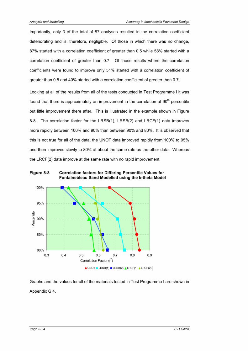
Analysis and Modelling Accuracy in Mechanistic Pavement Design
Page 8-24 S.D.Gillett
Importantly, only 3 of the total of 87 analyses resulted in the correlation coefficient
deteriorating and is, therefore, negligible. Of those in which there was no change,
87% started with a correlation coefficient of greater than 0.5 while 58% started with a
correlation coefficient of greater than 0.7. Of those results where the correlation
coefficients were found to improve only 51% started with a correlation coefficient of
greater than 0.5 and 40% started with a correlation coefficient of greater than 0.7.
Looking at all of the results from all of the tests conducted in Test Programme I it was
found that there is approximately an improvement in the correlation at 90th percentile
but little improvement there after. This is illustrated in the example shown in Figure
8-8. The correlation factor for the LRSB(1), LRSB(2) and LRCF(1) data improves
more rapidly between 100% and 90% than between 90% and 80%. It is observed that
this is not true for all of the data, the UNOT data improved rapidly from 100% to 95%
and then improves slowly to 80% at about the same rate as the other data. Whereas
the LRCF(2) data improve at the same rate with no rapid improvement.
Figure 8-8 Correlation factors for Differing Percentile Values for Fontainebleau Sand Modelled using the k-theta Model
80%
85%
90%
95%
100%
0.3 0.4 0.5 0.6 0.7 0.8 0.9Correlation Factor (r2)
Per
cent
ile
UNOT LRSB(1) LRSB(2) LRCF(1) LRCF(2)
Graphs and the values for all of the materials tested in Test Programme I are shown in
Appendix G.4.
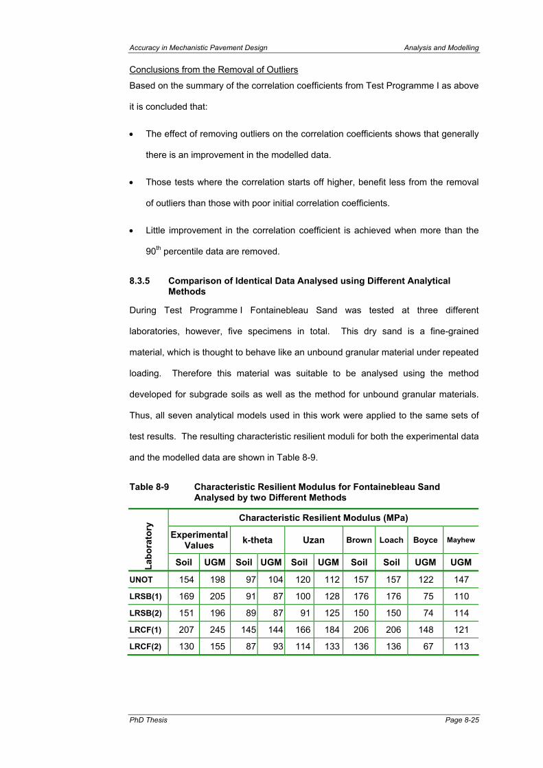
Accuracy in Mechanistic Pavement Design Analysis and Modelling
PhD Thesis Page 8-25
Conclusions from the Removal of Outliers
Based on the summary of the correlation coefficients from Test Programme I as above
it is concluded that:
• The effect of removing outliers on the correlation coefficients shows that generally
there is an improvement in the modelled data.
• Those tests where the correlation starts off higher, benefit less from the removal
of outliers than those with poor initial correlation coefficients.
• Little improvement in the correlation coefficient is achieved when more than the
90th percentile data are removed.
8.3.5 Comparison of Identical Data Analysed using Different Analytical Methods
During Test Programme I Fontainebleau Sand was tested at three different
laboratories, however, five specimens in total. This dry sand is a fine-grained
material, which is thought to behave like an unbound granular material under repeated
loading. Therefore this material was suitable to be analysed using the method
developed for subgrade soils as well as the method for unbound granular materials.
Thus, all seven analytical models used in this work were applied to the same sets of
test results. The resulting characteristic resilient moduli for both the experimental data
and the modelled data are shown in Table 8-9.
Table 8-9 Characteristic Resilient Modulus for Fontainebleau Sand Analysed by two Different Methods
Characteristic Resilient Modulus (MPa)
Experimental Values k-theta Uzan Brown Loach Boyce Mayhew
Labo
rato
ry
Soil UGM Soil UGM Soil UGM Soil Soil UGM UGM
UNOT 154 198 97 104 120 112 157 157 122 147
LRSB(1) 169 205 91 87 100 128 176 176 75 110
LRSB(2) 151 196 89 87 91 125 150 150 74 114
LRCF(1) 207 245 145 144 166 184 206 206 148 121
LRCF(2) 130 155 87 93 114 133 136 136 67 113

Analysis and Modelling Accuracy in Mechanistic Pavement Design
Page 8-26 S.D.Gillett
The difference in the experimental values between the subgrade soil (Soil) and the
Unbound Granular Material (UGM) is due to the different characteristic stresses
applied to the equation. This shows the stress dependency of the material since the
UGM, which is higher in the pavement, has greater applied stresses and consequently
a higher resilient modulus than the subgrade soil which is lower in the pavement
structure. Similarly, it is expected that the modelled values for the material analysed
as a subgrade soil should be consistently lower than those for an unbound granular
material. This is true for the experimental values and the simpler k-theta and Uzan
models but not so for the more complex models. As a result of this the following
analysis does not combine the results obtained using the soil and UGM models.
Two comparisons can be made from these results namely:
• To compare the range of the resulting resilient moduli obtained from the different
model analysis using the results from a single laboratory’s data, and;
• To compare the resulting resilient moduli obtained from a single model analysis
type (for example k-theta) using the results from all of the laboratory’s data.
The average, and the range, of modelled resilient moduli can thus be compared
against one another and the characteristic experimental values for both comparisons.
These two comparisons are shown graphically in Figure 8-9 and Figure 8-10. In the
characteristic experimental resilient modulus for each specimen tested (different
laboratories) is shown as a point. So too is the average modelled value, however this
point has an error bar included so depict the range of all of the modelled values.
Figure 8-9 clearly shows that when the results are analysed using the subgrade soil
models that the experimental value is approximately equal to the upper limit of the
range of the characteristic values obtained from the models. For each specimen the
experimental value for the UGM is greater than the experimental value for the soil.
However, the reverse is true for the average resilient modulus when predicted using
the models. Further, the values predicted using the soil models show a greater
variation than those of the UGM models.

Accuracy in Mechanistic Pavement Design Analysis and Modelling
PhD Thesis Page 8-27
When the results from each specimen as analysed by a particular model are shown
as an average and range in Figure 8-10 it can be seen that again the modelled values
are lower than the experimental values.
Figure 8-9 Comparison of Fontainebleau Sand Results Analysed for Different Specimens (Laboratories)
50
100
150
200
250
UNOT
LRSB(1)
LRSB(2)
LRCF(1)
LRCF(2)
Cha
ract
eris
tic R
esilie
nt M
odul
us R
ange
(MPa
Subgrade Soil Unbound Granular Material
MrcMre
MrcMre
MrcMre
MrcMre
MrcMre
MrcMre
MrcMreMrcMre
MrcMre
MrcMre
Figure 8-10 Comparison of Fontainebleau Sand Results Analysed by Different Analytical Methods
50
100
150
200
250
Expe
rimen
tal
(soi
l)
k-th
eta
(soi
l)
Uza
n (s
oil)
Brow
n
Loac
h
Expe
rimen
tal
(UG
M)
k-th
eta
(UG
M)
Uza
n (U
GM
)
Boyc
e
May
hew
Cha
ract
eris
tic R
esili
ent M
odul
us R
ange
(MPa
)
Subgrade Soil Unbound Granular Material
The k-theta models yield similar results for different levels of stress (i.e. when
analysed as soil or as UGM), however Uzan varies somewhat with UGM yielding
Analysis and Modelling Accuracy in Mechanistic Pavement Design
Page 8-28 S.D.Gillett
higher values than soils. Brown and Loach predict the highest values but these are
similar to the experimental values. In general, the UGM models predict lower values
than the soils. The variation of resilient modulus between the different specimens
(laboratories) when analysed by the different methods for soils and UGM is between -
21% and 44%. The variation of resilient modulus between the model methods for all
specimens (laboratories) for soils and UGM and the average values are shown in
Table 8-10.
Table 8-10 Variation of Resilient Moduli when Predicted by Different Methods of Modelling
Model Soil Models UGM Models Both Models
Average 137 MPa 114 MPa 126 MPa
Variation Min Max Range Min Max Range Min Max Range
Specimens -20% 32% 51% -22% 30% 53% -21% 44% 64%
Models -26% 20% 46% -15% 19% 34% -23% 31% 54%
Therefore greater variation occurs between the resilient moduli as predicted from
analysing the results from a single specimen (laboratory) using different models than
there is when the results from different specimens are analysed using a single model.
8.3.6 Comparison of the Same Material Tested at Different Laboratories
After considering the results from Test Programme I, a second test programme was
formulated in order that the results from different laboratories testing similar materials
could be compared. Two materials were tested at four laboratories, one subgrade soil
– London Clay and the other an unbound granular material - Microgranite. The test
procedure for the soil required few stress paths and therefore no stress paths
(outliers) were excluded. However, there were substantially more stress paths
applied to the unbound granular material specimens and an analysis was conducted
for all of the data (100th percentile) and the 90th percentile data. Complete results of
the analysis are contained in the tables below and Appendix G. These results are
shown graphically in Figure 8-11 and Figure 8-12, which provide a graphic
representation of the difference in the results from the various laboratories.
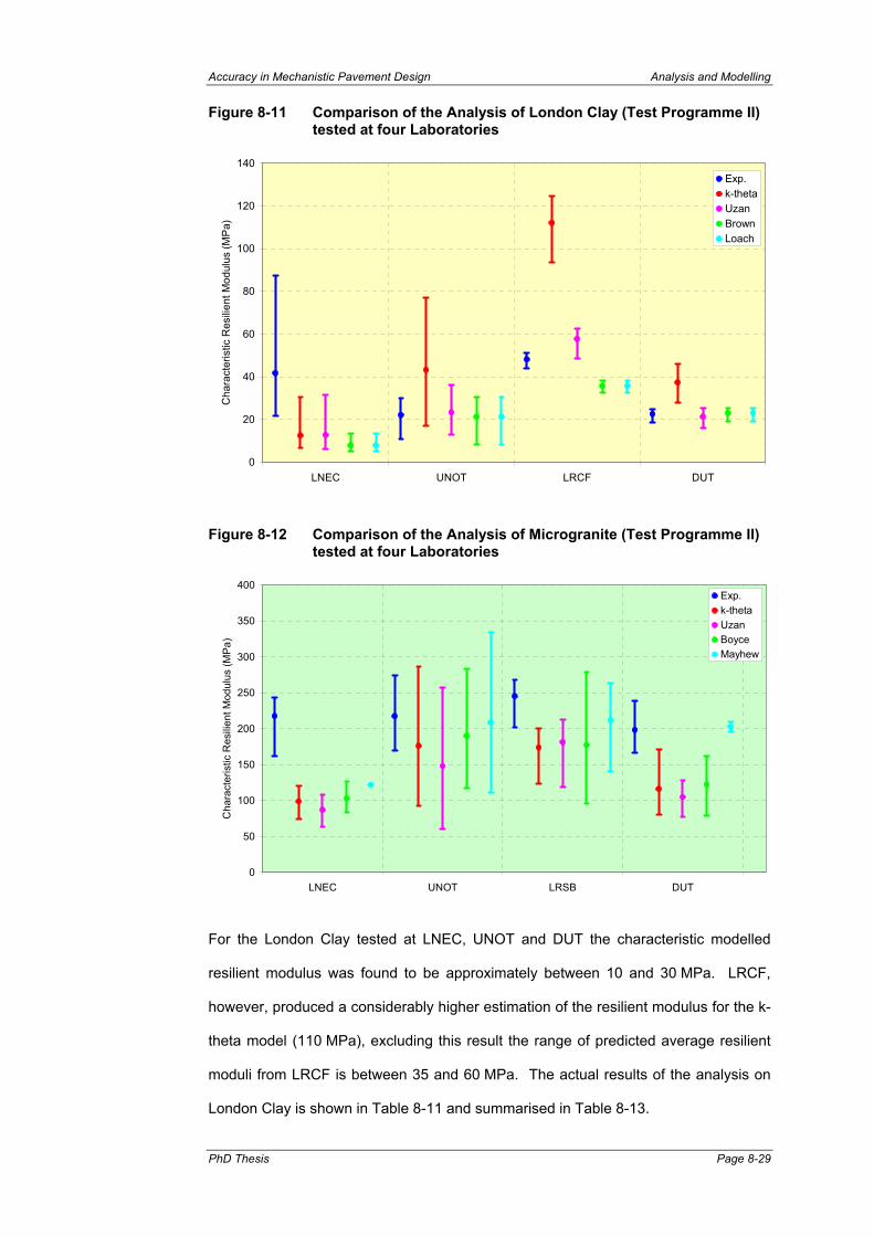
Accuracy in Mechanistic Pavement Design Analysis and Modelling
PhD Thesis Page 8-29
Figure 8-11 Comparison of the Analysis of London Clay (Test Programme II) tested at four Laboratories
0
20
40
60
80
100
120
140
LNEC UNOT LRCF DUT
Cha
ract
eris
tic R
esili
ent M
odul
us (M
Pa)
Exp.k-thetaUzanBrownLoach
Figure 8-12 Comparison of the Analysis of Microgranite (Test Programme II) tested at four Laboratories
0
50
100
150
200
250
300
350
400
LNEC UNOT LRSB DUT
Cha
ract
eris
tic R
esili
ent M
odul
us (M
Pa)
Exp.k-thetaUzanBoyceMayhew
For the London Clay tested at LNEC, UNOT and DUT the characteristic modelled
resilient modulus was found to be approximately between 10 and 30 MPa. LRCF,
however, produced a considerably higher estimation of the resilient modulus for the k-
theta model (110 MPa), excluding this result the range of predicted average resilient
moduli from LRCF is between 35 and 60 MPa. The actual results of the analysis on
London Clay is shown in Table 8-11 and summarised in Table 8-13.

Analysis and Modelling Accuracy in Mechanistic Pavement Design
Page 8-30 S.D.Gillett
Table 8-11 Results of Test Programme II on Subgrade Soil – London Clay
Modelled Values (MPa) Experimental Values k-theta Uzan Brown Loach Laboratory
Mre υe Mrc Mrc Mrc Mrc
22 0.54 7 6 5 5
24 0.67 9 9 6 6
59 0.74 12 12 10 10
28 0.64 9 9 7 7
30 1.19 8 8 6 6
LNEC
88 3.13 30 32 13 13
Min 22 0.54 7 6 5 5
Avg 42 1.15 13 13 8 8
Max 88 3.13 30 32 13 13
11 0.78 77 31 8 8
23 0.57 46 17 18 18
29 0.81 55 27 29 29
19 0.39 17 13 20 20
30 0.42 43 36 31 31
UNOT
21 1.10 21 16 22 22
Min 11 0.39 17 13 8 8
Avg 22 0.68 43 23 21 21
Max 30 1.10 77 36 31 31
51 0.76 118 62 38 38
49 0.86 125 63 37 37 LRCF
44 0.60 94 49 32 32
Min 44 0.60 94 49 32 32
Avg 48 0.74 112 58 36 36
Max 51 0.86 125 63 38 38
18 0.37 28 16 19 19
24 0.39 38 23 25 25 DUT
25 0.49 46 25 25 25
Min 18 0.37 28 16 19 19
Avg 23 0.42 37 21 23 23
Max 25 0.49 46 25 25 25

Accuracy in Mechanistic Pavement Design Analysis and Modelling
PhD Thesis Page 8-31
Table 8-12 Results of Test Programme II on Unbound Granular Material - Microgranite
Modelled Values (MPa) ExperimentalValues k-theta Uzan Boyce Mayhew Laboratory
Mre υe Mrc Mrc Mrc υc Mrc υc
162 0.2 85 78 88 -0.4
194 0.4 75 63 83 -0.1
244 0.1 120 104 107 -0.7
244 0.2 92 83 127 0.9
238 0.2 115 108 111 -0.3 122 0.4
LNEC
225 0.1 108 89 102 -0.4
Min 162 0.1 75 63 83 -0.7 122 0.4
Avg 218 0.2 99 87 103 -0.2 122 0.4
Max 244 0.4 120 108 127 0.9 122 0.4
169 0.2 94 61 117 0.5 112 0.4
274 0.4 287 257 284 -1.0 334 0.5 UNOT
210 0.5 149 126 170 -0.2 181 0.5
Min 169 0.2 94 61 117 -1.0 112 0.4
Avg 218 0.4 177 148 190 -0.2 209 0.5
Max 274 0.5 287 257 284 0.5 334 0.5
266 0.3 200 213 279 0.0 231 -0.1
268 0.4 198 212 156 -1.0 263 0.4 LRSB
202 0.4 123 119 96 -0.8 141 0.4
Min 202 0.3 123 119 96 -1.0 141 -0.1
Avg 245 0.3 174 181 177 -0.6 212 0.2
Max 268 0.4 200 213 279 0.0 263 0.4
239 0.2 172 129 163 -0.9
189 0.2 96 109 126 -0.4 210 0.1 DUT
167 0.2 81 77 79 -0.8 196 0.7
Min 167 0.2 81 77 79 -0.9 196 0.1
Avg 198 0.2 116 105 123 -0.7 203 0.4
Max 239 0.2 172 129 163 -0.4 210 0.7
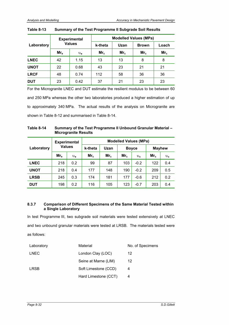
Analysis and Modelling Accuracy in Mechanistic Pavement Design
Page 8-32 S.D.Gillett
Table 8-13 Summary of the Test Programme II Subgrade Soil Results
Modelled Values (MPa) Experimental Values k-theta Uzan Brown Loach Laboratory
Mre υe Mrc Mrc Mrc Mrc
LNEC 42 1.15 13 13 8 8
UNOT 22 0.68 43 23 21 21
LRCF 48 0.74 112 58 36 36
DUT 23 0.42 37 21 23 23
For the Microgranite LNEC and DUT estimate the resilient modulus to be between 60
and 250 MPa whereas the other two laboratories produced a higher estimation of up
to approximately 340 MPa. The actual results of the analysis on Microgranite are
shown in Table 8-12 and summarised in Table 8-14.
Table 8-14 Summary of the Test Programme II Unbound Granular Material – Microgranite Results
Modelled Values (MPa) Experimental Values k-theta Uzan Boyce Mayhew Laboratory
Mre υe Mrc Mrc Mrc υc Mrc υc
LNEC 218 0.2 99 87 103 -0.2 122 0.4
UNOT 218 0.4 177 148 190 -0.2 209 0.5
LRSB 245 0.3 174 181 177 -0.6 212 0.2
DUT 198 0.2 116 105 123 -0.7 203 0.4
8.3.7 Comparison of Different Specimens of the Same Material Tested within a Single Laboratory
In test Programme III, two subgrade soil materials were tested extensively at LNEC
and two unbound granular materials were tested at LRSB. The materials tested were
as follows:
Laboratory Material No. of Specimens
LNEC London Clay (LOC) 12
Seine at Marne (LIM) 12
LRSB Soft Limestone (CCD) 4
Hard Limestone (CCT) 4
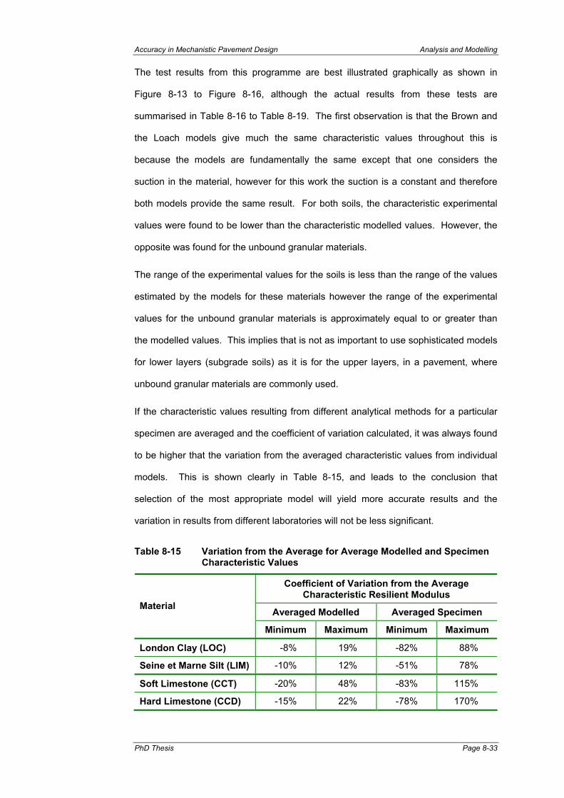
Accuracy in Mechanistic Pavement Design Analysis and Modelling
PhD Thesis Page 8-33
The test results from this programme are best illustrated graphically as shown in
Figure 8-13 to Figure 8-16, although the actual results from these tests are
summarised in Table 8-16 to Table 8-19. The first observation is that the Brown and
the Loach models give much the same characteristic values throughout this is
because the models are fundamentally the same except that one considers the
suction in the material, however for this work the suction is a constant and therefore
both models provide the same result. For both soils, the characteristic experimental
values were found to be lower than the characteristic modelled values. However, the
opposite was found for the unbound granular materials.
The range of the experimental values for the soils is less than the range of the values
estimated by the models for these materials however the range of the experimental
values for the unbound granular materials is approximately equal to or greater than
the modelled values. This implies that is not as important to use sophisticated models
for lower layers (subgrade soils) as it is for the upper layers, in a pavement, where
unbound granular materials are commonly used.
If the characteristic values resulting from different analytical methods for a particular
specimen are averaged and the coefficient of variation calculated, it was always found
to be higher that the variation from the averaged characteristic values from individual
models. This is shown clearly in Table 8-15, and leads to the conclusion that
selection of the most appropriate model will yield more accurate results and the
variation in results from different laboratories will not be less significant.
Table 8-15 Variation from the Average for Average Modelled and Specimen Characteristic Values
Coefficient of Variation from the Average Characteristic Resilient Modulus
Averaged Modelled Averaged Specimen Material
Minimum Maximum Minimum Maximum
London Clay (LOC) -8% 19% -82% 88%
Seine et Marne Silt (LIM) -10% 12% -51% 78%
Soft Limestone (CCT) -20% 48% -83% 115%
Hard Limestone (CCD) -15% 22% -78% 170%

Analysis and Modelling Accuracy in Mechanistic Pavement Design
Page 8-34 S.D.Gillett
Table 8-16 Results of Test Programme III on Subgrade Soil – London Clay
Modelled Values (MPa) Experimental Values k-theta Uzan Brown Loach Material
Mre υe Mrc Mrc Mrc Mrc
232 0.26 447 401 401
180 0.33 352 241 241
108 0.31 275 186 154 154
84 0.26 153 109 100 100
124 0.26 232 167 145 145
95 0.30 148 122 105 105
199 0.50 318 252 252
136 0.49 255 175 175
328 0.53 416 416
93 0.22 33 44 44
204 0.26 506 246 246
LOC
153 0.21 496 164 167 167
Min 84 0.21 33 109 44 44
10% 93 0.22 91 121 100 100
Avg 161 0.33 223 263 204 204
90% 229 0.50 385 453 386 386
Max 328 0.53 496 506 416 416
Figure 8-13 Analysis of the London Clay Specimens tested at LNEC under Test Programme III
0
100
200
300
400
500
600
Exp. k-theta Uzan Brown Loach
Cha
ract
eris
tic R
esili
ent M
odul
us (M
Pa)

Accuracy in Mechanistic Pavement Design Analysis and Modelling
PhD Thesis Page 8-35
Table 8-17 Results of Test Programme III on Subgrade Soil – Seine et Marne Silt
Modelled Values (MPa) Experimental Values k-theta Uzan Brown Loach Material
Mre υe Mrc Mrc Mrc Mrc
213 0.24 245 175 220 220
217 0.22 204 189 214 214
195 0.24 284 185 224 224
134 0.20 103 91 138 138
132 0.52 244 253 141 141
216 0.42 141 137 252 252
144 0.34 102 108 154 154
398 0.69 409 319 483 483
184 0.22 345 245 238 238
203 0.27 336 297 237 237
269 0.22 470 321 334 334
LIM
152 0.27 296 247 189 189
Min 132 0.20 102 91 138 138
10% 135 0.22 107 111 143 143
Avg 205 0.32 265 214 235 235
90% 264 0.51 402 317 326 326
Max 398 0.69 470 321 483 483
Figure 8-14 Analysis of the Seine et Marne Specimens Tested at LNEC under Test Programme III
0
100
200
300
400
500
600
Exp. k-theta Uzan Brown Loach
Cha
ract
eris
tic R
esili
ent M
odul
us (M
Pa)
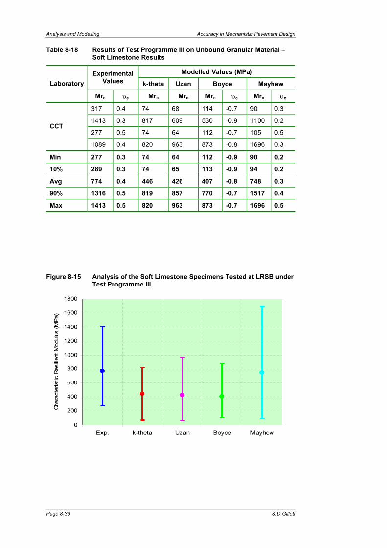
Analysis and Modelling Accuracy in Mechanistic Pavement Design
Page 8-36 S.D.Gillett
Table 8-18 Results of Test Programme III on Unbound Granular Material – Soft Limestone Results
Modelled Values (MPa) Experimental Values k-theta Uzan Boyce Mayhew Laboratory
Mre υe Mrc Mrc Mrc υc Mrc υc
317 0.4 74 68 114 -0.7 90 0.3
1413 0.3 817 609 530 -0.9 1100 0.2
277 0.5 74 64 112 -0.7 105 0.5 CCT
1089 0.4 820 963 873 -0.8 1696 0.3
Min 277 0.3 74 64 112 -0.9 90 0.2
10% 289 0.3 74 65 113 -0.9 94 0.2
Avg 774 0.4 446 426 407 -0.8 748 0.3
90% 1316 0.5 819 857 770 -0.7 1517 0.4
Max 1413 0.5 820 963 873 -0.7 1696 0.5
Figure 8-15 Analysis of the Soft Limestone Specimens Tested at LRSB under Test Programme III
0
200
400
600
800
1000
1200
1400
1600
1800
Exp. k-theta Uzan Boyce Mayhew
Cha
ract
eris
tic R
esili
ent M
odul
us (M
Pa)

Accuracy in Mechanistic Pavement Design Analysis and Modelling
PhD Thesis Page 8-37
Table 8-19 Results of Test Programme III on Unbound Granular Material – Hard Limestone Results
Modelled Values (MPa) ExperimentalValues k-theta Uzan Boyce Mayhew Laboratory
Mre υe Mrc Mrc Mrc υc Mrc υc
1586 0.6 1388 1273 1929 -0.1 1436 0.2
536 0.3 177 157 344 0.2 305 0.2
354 0.7 100 94 170 0.5 124 0.5 CCD
794 0.2 238 285 -0.6 341 0.1
Min 354 0.2 100 94 170 -0.6 124 0.1
10% 409 0.3 124 107 205 -0.4 178 0.1
Avg 817 0.5 476 381 682 0.0 552 0.2
90% 1348 0.7 1043 938 1453 0.4 1108 0.4
Max 1586 0.7 1388 1273 1929 0.5 1436 0.5
Figure 8-16 Analysis of the Hard Limestone Specimens Tested at LRSB under Test Programme III
0
200
400
600
800
1000
1200
1400
1600
1800
2000
Exp. k-theta Uzan Boyce Mayhew
Cha
ract
eris
tic R
esili
ent M
odul
us (M
Pa)

Analysis and Modelling Accuracy in Mechanistic Pavement Design
Page 8-38 S.D.Gillett
8.4 INTRODUCTION OF RANDOM ERRORS TO DATA
In order to test the influence that errors in the readings from the instrumentation have
on the modelling and pavement design, a controlled error was introduced into what
was otherwise ‘perfect data’.
Two materials, an unbound granular material (CCT) and a subgrade soil (LOC) were
selected and the strains calculated using a simple model as follows:
( ) ( )
( ) ( )3ra1a1r3
1r22a1
Fνενεε
VFbqabqaε
××+×=
××+×++×= Eqn.8-2
Where Fr Random number between -1 and 1 (subscript indicated axial and radial) V Variation a and b Constants dependent on actual measurements ν Poisson’s ratio (assumed constant) = 0.40
The coefficients for the models were calculated, as before, for different values of
variation, (0%; 2%; 5%; 10%; 30%; 50%), for both the CCT and the LOC. Figure 8-17
and Figure 8-18 show the scatter of the points increasing as the variation increases
for the two examples.
It was found that the introduction of a random error and the subsequent increase in
the variation had very little effect on the material coefficients for variation of up to 30%
for both materials and thus modelling methods. There was a ‘jump’ in the magnitude
of the parameters and coefficients at 50% variation, however. All of the results of this
model analysis can be found in Appendix G Also summary tables containing the
material parameters and coefficients are contained in this appendix.

Analysis and Modelling Accuracy in Mechanistic Pavement Design
PhD Thesis Page 8-39
Figure 8-17 Increase in Scatter as the Variation Increases for a Subgrade Soil
Variation = 0%
0
20
40
60
80
100
120
140
160
0 20 40 60 80 100 120 140 160Experimental [Mr] (MPa)
Mod
elle
d [M
r] (M
Pa)
k-thetaUzanBrownLoach
Variation = 5%
0
20
40
60
80
100
120
140
160
0 20 40 60 80 100 120 140 160Experimental [Mr] (MPa)
Mod
elle
d [M
r] (M
Pa)
Variation = 30%
0
20
40
60
80
100
120
140
160
0 20 40 60 80 100 120 140 160Experimental [Mr] (MPa)
Mod
elle
d [M
r] (M
Pa)
Variation = 50%
0
20
40
60
80
100
120
140
160
0 20 40 60 80 100 120 140 160Experimental [Mr] (MPa)
Mod
elle
d [M
r] (M
Pa)

Analysis and Modelling Accuracy in Mechanistic Pavement Design
S.D.Gillett Page 8-40
Figure 8-18 Increase in Scatter as the Variation Increases for an Unbound Granular Material
Variation = 0%
0
500
1,000
1,500
2,000
2,500
3,000
0 500 1,000 1,500 2,000 2,500 3,000Experimental [Mr] (MPa)
Mod
elle
d [M
r] (M
Pa)
k-thetaUzanBoyceMayhew
Variation = 5%
0
500
1,000
1,500
2,000
2,500
3,000
0 500 1,000 1,500 2,000 2,500 3,000Experimental [Mr] (MPa)
Mod
elle
d [M
r] (M
Pa)
Variation = 30%
0
500
1,000
1,500
2,000
2,500
3,000
0 500 1,000 1,500 2,000 2,500 3,000Experimental [Mr] (MPa)
Mod
elle
d [M
r] (M
Pa)
Variation = 50%
0
500
1,000
1,500
2,000
2,500
3,000
0 500 1,000 1,500 2,000 2,500 3,000Experimental [Mr] (MPa)
Mod
elle
d [M
r] (M
Pa)
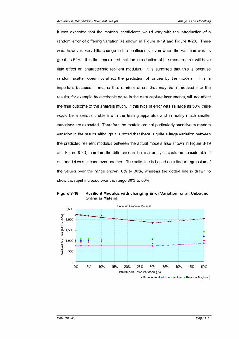
Accuracy in Mechanistic Pavement Design Analysis and Modelling
PhD Thesis Page 8-41
It was expected that the material coefficients would vary with the introduction of a
random error of differing variation as shown in Figure 8-19 and Figure 8-20. There
was, however, very little change in the coefficients, even when the variation was as
great as 50%. It is thus concluded that the introduction of the random error will have
little effect on characteristic resilient modulus. It is surmised that this is because
random scatter does not affect the prediction of values by the models. This is
important because it means that random errors that may be introduced into the
results, for example by electronic noise in the data capture instruments, will not affect
the final outcome of the analysis much. If this type of error was as large as 50% there
would be a serious problem with the testing apparatus and in reality much smaller
variations are expected. Therefore the models are not particularly sensitive to random
variation in the results although it is noted that there is quite a large variation between
the predicted resilient modulus between the actual models also shown in Figure 8-19
and Figure 8-20, therefore the difference in the final analysis could be considerable if
one model was chosen over another. The solid line is based on a linear regression of
the values over the range shown, 0% to 30%, whereas the dotted line is drawn to
show the rapid increase over the range 30% to 50%.
Figure 8-19 Resilient Modulus with changing Error Variation for an Unbound Granular Material
Unbound Granular Material
0
500
1,000
1,500
2,000
2,500
0% 5% 10% 15% 20% 25% 30% 35% 40% 45% 50%
Introduced Error Variation (%)
Res
ilient
Mod
ulus
[Mrc
] (M
Pa)
Experimental k-theta Uzan Boyce Mayhew

Analysis and Modelling Accuracy in Mechanistic Pavement Design
Page 8-42 S.D.Gillett
Figure 8-20 Resilient Modulus with changing Error Variation for a Subgrade Soil
Subgrade Soil
0
50
100
150
200
250
300
0% 5% 10% 15% 20% 25% 30% 35% 40% 45% 50%
Introduced Error Variation (%)
Res
ilient
Mod
ulus
[Mrc
] (M
Pa)
Experimental k-theta Uzan Brown Loach
8.5 FINAL VALUES FROM THE TESTING AND ANALYSIS
The final results from all three test programmes (material parameters and material
coefficients) are used to analyse typical pavements in the next chapter.
The method of data verification and eliminating the outliers remains as discussed
earlier. In all cases the material parameters are shown as an average of the verified
data results and a 10th and 90th percentile value of the data. For Test Programme I,
where a single specimen was tested at each laboratory, the results are quoted by
material since they were calculated by taking the average values of all specimens and
the deviation is taken as the 10th and 90th percentile values regardless of laboratory.
For the other two test programmes, where more than one specimen was tested, for
each material, at different laboratories, the results are quoted first by material then by
laboratory and never combined. The final results of the analysis yielding the values
and ranges of the parameters and coefficients, for the three test programmes, for all of
the subgrade soils tested, are shown in Table 8-20 and for all of the unbound granular
materials tested are shown in Table 8-21.

Analysis and Modelling Accuracy in Mechanistic Pavement Design
PhD Thesis Page 8-43
Table 8-20 Final Parameters and Coefficients for the Subgrade Soils
Modelled Valuesk-theta Uzan Brown Loach
Mre υe Mrc k1 k2 Mrc k3 k4 k5 Mrc A B Mrc C DLower 10% 138 0.28 82 126,079 0.4037 99 226,959 0.2570 0.2145 147 84,026 -0.2594 147 2,843,389 0.7459SFB All 160 0.41 96 143,380 0.3842 119 244,958 0.2226 0.1938 172 98,734 -0.2581 170 3,184,624 0.7333
Upper 90% 190 0.55 117 170,183 0.3541 142 267,203 0.1799 0.1682 202 116,376 -0.2566 196 3,571,066 0.7191Lower 10% 23 0.53 33 28,851 -0.1559 20 10,465 0.1227 -0.6767 21 17,515 0.4508 21 43,787 1.4508LOC All 34 0.54 45 33,040 -0.2594 30 14,036 -0.0284 -0.4879 27 21,858 0.4820 27 54,645 1.4820
Upper 90% 44 0.56 61 38,750 -0.4004 42 18,458 -0.2155 -0.2540 31 25,304 0.5068 31 63,260 1.5068Lower 10% 6 0.51 8 4,429 -0.5620 7 2,409 -0.6398 0.1226 6 5,110 0.2186 6 12,774 1.2186LOC LNEC 8 0.53 13 5,177 -0.7242 13 2,252 -0.7694 0.0458 8 6,587 0.3682 8 16,467 1.3682
Upper 90% 12 0.58 21 6,461 -1.0026 22 1,988 -0.9882 -0.0836 12 8,870 0.5993 12 22,174 1.5993Lower 10% 15 0.41 19 23,542 0.1559 14 13,352 0.2010 -0.5256 13 9,871 0.8931 13 24,678 1.8931LOC UNOT 22 0.68 43 21,273 -0.6034 23 12,518 -0.1223 -0.6058 21 17,512 0.5781 21 43,781 1.5781
Upper 90% 29 0.96 66 19,132 -1.3199 34 11,584 -0.4841 -0.6955 30 25,480 0.2496 30 63,700 1.2496Lower 10% 45 0.63 99 40,556 -0.8336 51 11,351 -0.2865 -0.6545 33 24,152 0.7310 33 60,381 1.7310LOC LRCF 48 0.74 112 43,376 -0.8888 58 11,597 -0.3231 -0.6660 36 25,647 0.7567 36 64,117 1.7567
Upper 90% 51 0.84 123 45,699 -0.9343 63 11,785 -0.3510 -0.6748 38 26,922 0.7786 38 67,304 1.7786Lower 10% 20 0.37 30 17,492 -0.5121 17 6,637 0.1141 -0.8923 20 13,887 0.8442 20 34,718 1.8442LOC DUT 23 0.42 37 19,736 -0.5906 21 6,866 0.0662 -0.9380 23 15,533 0.8972 23 38,832 1.8972
Upper 90% 25 0.47 44 21,873 -0.6654 25 7,061 0.0255 -0.9767 25 16,738 0.9360 25 41,844 1.9360Lower 10% 93 0.22 91 54,817 -0.3212 121 60,030 -0.1499 -0.3988 100 86,325 0.3546 100 215,813 1.3546
25% 105 0.26 149 73,617 -0.4512 165 61,451 -0.1815 -0.4510 135 106,367 0.4438 135 265,916 1.4438LOC LNEC 161 0.33 223 97,303 -0.6150 263 64,625 -0.2520 -0.5675 204 146,365 0.6219 204 365,911 1.6219
75% 200 0.37 264 110,590 -0.7069 344 67,249 -0.3103 -0.6638 247 171,613 0.7343 247 429,033 1.7343Upper 90% 229 0.50 385 149,561 -0.9764 453 70,800 -0.3891 -0.7942 386 252,161 1.0930 386 630,402 2.0930Lower 10% 141 0.22 111 126,210 0.0348 126 147,830 0.2086 -0.3514 150 106,795 0.4005 150 133,494 1.4005
LIM LNEC 226 0.32 275 187,006 -0.3015 328 135,299 -0.1238 -0.3973 247 135,632 0.5575 247 169,540 1.5575Upper 90% 337 0.45 406 235,484 -0.5696 669 114,132 -0.6853 -0.4749 340 163,230 0.7077 340 204,037 1.7077
Test
Prog
ram
me
IITe
stPr
ogra
mm
e III
ExperimentalValuesMat. Lab.
Test
Prog
ram
me
I
TestPgm.

Analysis and Modelling Accuracy in Mechanistic Pavement Design
S.D.Gillett Page 8-44
Table 8-21 Final Parameters and Coefficients for the Unbound Granular Materials
Modelled Valuesk-theta Uzan Boyce Mayhew
Mre υe Mrc k1 k2 Mrc k3 k4 k5 Mrc υc Ga Ka n Mrc υc Ga Ka n b mLower 10% 171 0.25 87 122,206 0.4363 117 227,011 0.2989 0.1446 90 -0.19 63,350 36,141 0.2428 111 0.27 62,075 59,651 0.2560 0.0411 0.4130SFB All 200 0.35 103 140,508 0.4069 137 246,351 0.2635 0.1614 115 0.27 82,980 115,073 0.4006 121 0.47 78,350 217,163 0.3495 0.2813 0.7975
Upper 90% 229 0.48 128 168,708 0.3617 164 273,733 0.2135 0.1853 140 0.78 112,838 233,881 0.5083 137 0.64 88,664 473,408 0.4547 0.5892 1.2997Lower 10% 452 0.33 236 364,985 0.5642 232 799,759 0.7274 -0.0900 180 -0.50 154,908 43,918 0.1123 207 0.59 160,537 21,295 0.0258 0.0409 0.1335CCD All 554 0.40 311 416,892 0.4017 388 692,114 0.3126 0.1291 278 0.12 355,030 320,449 0.2978 269 0.62 172,857 97,841 0.2035 0.1969 0.6514
Upper 90% 640 0.49 389 470,910 0.2326 525 597,979 -0.0502 0.3206 384 0.58 610,552 678,945 0.5216 332 0.66 185,178 174,388 0.3813 0.3529 1.1692Lower 10% 443 0.45 331 389,012 0.2805 420 505,501 0.2014 0.1199 397 -0.13 109,948 463,595 0.2437 359 0.27 104,399 972,395 -0.1005 0.0187 0.7252CCT All 1,131 0.46 930 1,026,881 0.2035 1,323 1,229,127 0.0392 0.1886 1,318 0.11 234,974 2,123,377 0.3579 1,248 0.37 235,460 1,655,747 0.1811 0.2425 1.7719
Upper 90% 1,820 0.47 1,529 1,664,750 0.1265 2,227 1,952,753 -0.1231 0.2573 2,240 0.35 360,001 3,783,159 0.4722 2,138 0.47 366,520 2,339,099 0.4627 0.4664 2.8185Lower 10% Only One Specimen TestedMIG All 235 0.28 79 133,321 0.6716 105 290,773 0.4896 0.1570 80 -0.24 114,963 11,175 0.0908 83 0.36 81,478 38,124 -0.0181 0.0595 0.1668
Upper 90% Only One Specimen Tested
Lower 10% 178 0.14 80 150,359 0.8095 71 395,080 0.9426 -0.1032 86 -0.57 156,579 -912,637 0.1636MIG LNEC 218 0.22 99 174,492 0.7339 87 405,646 0.8502 -0.0896 103 -0.17 162,213 977,178 0.1161 122 0.38 NS NS NS NS NS
Upper 90% 244 0.34 118 197,459 0.6620 106 417,387 0.7475 -0.0745 119 0.41 167,434 2,728,552 0.0721Lower 10% 178 0.27 105 149,260 0.4325 74 254,106 0.7245 -0.2347 128 -0.81 -40,182 99,005 0.3493 125 0.41 123,576 70,757 0.2570 0.4307 2.0112MIG UNOT 218 0.37 177 200,441 0.2430 148 262,752 0.4454 -0.1702 190 -0.23 622,015 69,324 0.6201 209 0.47 113,473 73,211 0.4367 0.4739 1.9558
Upper 90% 261 0.46 259 259,432 0.0247 231 272,428 0.1329 -0.0980 261 0.33 1,371,897 35,713 0.9268 303 0.51 102,005 75,997 0.6405 0.5231 1.8929Lower 10% 215 0.29 138 184,723 0.3810 138 278,660 0.3964 -0.0197 108 -0.92 756,369 16,035 0.4494 159 0.01 145,388 79,052 0.3563 0.1322 0.4563MIG LRSB 245 0.34 174 220,219 0.3140 181 306,985 0.2848 0.0358 177 -0.60 589,138 52,101 0.5499 212 0.25 187,846 89,619 0.4718 0.0966 0.5095
Upper 90% 267 0.38 200 246,030 0.2652 213 327,489 0.2041 0.0759 255 -0.19 401,550 92,557 0.6627 257 0.43 224,174 98,661 0.5707 0.0660 0.5550Lower 10% 172 0.22 84 144,478 0.6793 84 293,553 0.6691 0.0105 88 -0.89 200,064 19,602 0.2755 197 0.20 495,334 94,027 0.2560 -1.6121 -1.2948MIG DUT 198 0.23 116 173,821 0.5555 105 322,487 0.6268 -0.0618 123 -0.69 416,086 25,299 0.4091 203 0.44 285,341 94,187 0.3597 -0.8421 -0.5928
Upper 90% 229 0.24 157 210,544 0.4006 125 349,171 0.5877 -0.1285 155 -0.45 623,184 30,761 0.5372 209 0.68 75,349 94,348 0.4633 -0.0721 0.1092
Lower 10% 409 0.26 124 245,559 0.7461 28 318,306 1.0641 1.1616 205 -0.45 365,942 62,368 0.1864 178 0.15 3,385,321 201,533 0.1152 -0.2732 1.065025% 491 0.32 158 278,668 0.7269 71 376,649 1.0390 1.1029 257 -0.21 373,822 79,087 0.2079 260 0.16 3,179,554 219,591 0.1585 -0.2604 1.0460
CCD LRSB 817 0.48 476 581,965 0.5508 381 803,897 0.8549 0.6730 682 -0.01 438,631 216,573 0.3848 552 0.25 2,439,090 284,574 0.3142 -0.2147 0.977775% 992 0.64 525 629,116 0.5234 436 879,372 0.8223 0.5971 740 0.23 447,448 235,278 0.4088 615 0.27 2,278,385 298,677 0.3480 -0.2048 0.9628
Upper 90% 1,348 0.69 1,043 1,123,288 0.2365 938 1,570,905 0.5244 -0.0987 1,453 0.38 556,113 465,804 0.7055 1,108 0.41 1,029,050 408,318 0.6108 -0.1276 0.8475Lower 10% 289 0.31 74 132,897 0.7465 65 389,970 0.9163 -0.1992 113 -0.89 325,886 15,486 0.1250 94 0.21 -64,620 66,103 -0.1634 -0.5983 0.4258CCT LRSB 774 0.40 446 547,528 0.4772 426 753,290 0.5643 -0.0779 407 -0.79 673,201 69,736 0.3478 748 0.32 1,245,446 160,120 0.1411 -0.7012 0.5969
Upper 90% 1,316 0.46 819 962,829 0.2074 857 1,187,048 0.1441 0.0670 770 -0.69 1,100,861 136,536 0.6221 1,517 0.44 2,788,027 270,823 0.4996 -0.8224 0.7984
ExperimentalValues
Test
Pro
gram
me
ITe
st P
rogr
amm
e II
Test
Pro
g III
Mat. Lab.

Accuracy in Mechanistic Pavement Design Analysis and Modelling
PhD Thesis Page 8-45
8.6 SUMMARY
Constitutive relationships have been developed which attempt to model the behaviour
of road construction material under traffic loading. The analysis of repeated load
triaxial test data using these relationships yield material parameters and coefficients
that describe the material characteristics under traffic loading.
Some simple material relationships are generally used in practice. More often,
however, the material parameters (resilient modulus and Poisson’s ratio) are obtained
by unreliable relationships with empirical parameters or even just estimation with
guidance from publications.
Having logged the data from the repeated load triaxial tests a method of data
verification is proposed whereby all outliers are removed. Further, secondary
screening of the data, outside defined percentile variation, is also conducted. Based
on the removal of ‘outliers’ and the correlation of fit of the data the removal of the 10th
percentile data appears to be a good compromise resulting in an improved correlation
without the loss of too much data.
Analysis was conducted using a proprietary software package and a spreadsheet
containing the method of least squares curve-fitting analysis. The spreadsheet
provided a more robust method although it was limited in the statistical indicators
provided.
Numerous analyses were conducted for a range of road construction materials
resulting in the material properties (material parameters and model coefficients) being
produced. Some problems in determining a realistic solution were encountered and a
pragmatic set of rules (minimum and maximum values for the coefficients and
parameters) was formulated (shown in Table 8-4). This allowed the characterisation
of ‘good’ and ‘bad’ results, where the bad results were unrealistic and could be
removed.
It order to determine material coefficients for all eventualities the coefficients were
extrapolated for all values of characteristic resilient modulus for that particular sample,
based on a linear regression of all points. This has allowed coefficients to be

Analysis and Modelling Accuracy in Mechanistic Pavement Design
Page 8-46 S.D.Gillett
calculated for differing percentile values of the characteristic resilient modulus (i.e.
10%, 25% Average, 75% and 90%).
In general experimental values of resilient modulus for unbound granular materials
were higher than the corresponding characteristic values obtained from the models,
whereas for subgrade soils the opposite trend was observed. This implies that
incorrect characteristic stresses may have been assumed and since the materials are
stress dependent this could be corrected by increasing the characteristic stresses so
that the characteristic resilient moduli also increased.
As expected, different laboratories, testing the same material, have resulted in
different characteristic material properties. Also there is a difference in the results
between specimens tested in the same laboratory at each of the four laboratories.
The significance of these differences will be discussed in the next chapter.

Accuracy in Mechanistic Pavement Design Mechanistic Pavement Design
PhD Thesis Page 9-1
9 DESIGN OF FLEXIBLE PAVEMENTS USING THE TEST RESULTS
9.1 INTRODUCTION
It was stated in an earlier chapter that the mechanistic design or analysis of flexible
pavements refers to the numerical calculation of the deflection, stress and strain in a
multi-layered pavement, when subjected to external loads, and the subsequent
translation of these analytical calculations of pavement response into a prediction of
the performance of the pavement.
During a parametric study Dawson and Plaistow (1993), analysing thinly surfaced
flexible pavements using finite element analysis, suggested that a more detailed
representation of granular material, in structurally significant unbound pavement
layers would lead to more efficient (and thus more economical) pavement structures.
As has been discussed, it is well recognised the road construction materials are non-
linear stress dependent anisotropic materials. Therefore it is best to characterise the
material, by defining the material parameters in a model under realistic loading
conditions. With the advent of powerful personal computers, the use of finite element
analysis computer programs is one such technique.
Two computer analysis programs are used for this work. The first, ELSYM5 {Ahlborn
(1963)}, is a commonly used simple non-linear multi-layer analysis program and the
second is the more complex finite element analysis method used by FENLAP
{Almeida (1991)} and developed at the University of Nottingham.
FENLAP is able to model the non-linearity of the layers, while in ELSYM5 (PC
version) it is possible to simulate some non-linearity into a single layer by splitting the
layer up into thinner layers and allocating different values of the material parameters
at each layer. This program was, written some time ago, however, and it is unable to
cope with more than five layers and this restricts it applicability somewhat.
The outputs are the same for each analytical program; namely strains and stresses at
certain locations throughout the pavement structure. Typical European pavement
structures have been chosen to undertake this analysis. These were defined during

Mechanistic Pavement Design Accuracy in Mechanistic Pavement Design
Page 9-2 S.D.Gillett
the ‘Science Project’. The pavement structures and the points of analysis for the
ELSYM computer analytical program are shown in Figure 9-1 and the analysis grid (as
required for finite element analysis) for the FENLAP program is shown in Figure 9-2.
Figure 9-1 Analytical Points for ELSYM5 The Linear Elastic ELSYM Analysis Points
0.00 0.16 0.20 0.30 0.50 0.75 1 2 3 5 m
Pressure = 520 kPa
0 Linear Mr50 Elastic ν
150
Linear MrElastic ν
300
450
Linear MrElastic ν
600
750
Linear MrElastic ν
1,750
Linear MrElastic ν
Points where analysis was conducted
Soil
Sele
cted
Sub
grad
eIn
-Situ
Sub
grad
eA
spha
lt Su
rfac
e
150
mm
300
mm
300
mm
Gra
nula
r Bas
eG
ranu
lar S
ubba
se
1000
mm
1000

Accuracy in Mechanistic Pavement Design Mechanistic Pavement Design
PhD Thesis Page 9-3
Figure 9-2 Analytical Grid for FENLAP The Finite Element Fenlap Analysis Grid
0.00 0.16 0.20 0.30 0.50 0.75 1 2 3 5 m
Pressure = 520 kPa
0 Linear Mr50 Elastic ν
Unit wt.Suction
150
k θ Model CoefficientsBoyce Unit wt.Mayhew Suction
300
450
k θ Model CoefficientsUnit wt.Suction
600
750
Loach Model CoefficientsUnit wt.SuctionFailure Criteria
1,750
Brown Model CoefficientsUnit wt.SuctionFailure Criteria
Linear Mr2 750 Half Space with a fixed Mr and n
1000
mm
1000
Soil
Sele
cted
Sub
grad
eIn
-Situ
Sub
grad
eA
spha
lt Su
rfac
e
150
mm
300
mm
300
mm
Gra
nula
r Bas
eG
ranu
lar S
ubba
se

Mechanistic Pavement Design Accuracy in Mechanistic Pavement Design
Page 9-4 S.D.Gillett
9.2 THE STRUCTURAL ANALYSIS OF SPECIFIC PAVEMENTS
The structural analysis of the pavement (determination of stresses and strains at
particular points in the pavement under traffic loading) is performed by entering
various data with respect to the pavement into an analytical computer program.
The required input is often, but not restricted to, the following:
• Number of layers and thickness (except for the lowest layer which is assumed to
be semi-infinite);
• Number of loads and co-ordinates (x,y), tyre pressure and/ or contact area radius;
• Material parameters and/ or model coefficients;
• Co-ordinates of points to be investigated (x,y,z).
Depending on the nature of the material of each layer and its corresponding
mechanism of behaviour, critical values of either stress or strain are selected as
discussed earlier.
In the previous chapter, the material parameter values and the coefficients for the
models that describe the material behaviour were determined. In order to compare
the results, the materials, or more specifically the specimens from each laboratory and
test programme, have been listed in order of characteristics resilient modulus as
shown in Table 9-1. For this analysis it is necessary to identify a ‘high quality’ material
from a ‘poor quality’ material and thus a ‘strong’ pavement structure, comprising high
quality material from a ‘weak’ pavement structure comprising weaker material. This
ranking is done by taking the higher characteristic resilient modulus to indicate better
quality material. It is therefore expected that higher characteristic resilient moduli are
found nearer the surface of the pavement structures, and also weaker pavements will
have lower resilient moduli than stronger pavements.
During a comparison of these values against the guidelines in Chapter 2 it can be
seen that SFB (granular material) and MIG have lower resilient moduli than expected.
For the SFB this is likely since this material is not a base quality material but a fine-
grained sand which has unbound granular properties. The reasons for the MIG

Accuracy in Mechanistic Pavement Design Mechanistic Pavement Design
PhD Thesis Page 9-5
showing these poor characteristics goes beyond the actual quality of the parent
material, i.e. that as quarried and crushed and the explanation for the poor quality of
this material may be that the unbound material has a poor particle size distribution or
high clay content (PI). The other two granular materials (CCD and CCT) are shown to
be medium to good quality base materials.
Table 9-1 Ranking of the Materials Tested in Terms of Quality
Test Programme Material Laboratory
Characteristic Resilient Modulus
[Mrc] (MPa)
Unbound Granular Materials
2 MIG DUT 198 Poor Quality
1 SFB All 200
2 MIG UNOT 218
2 MIG LNEC 218
1 MIG All 235
2 MIG LRSB 245
1 CCD All 554
3 CCT LRSB 774
3 CCD LRSB 817
1 CCT All 1131 Good Quality
Subgrade Soils
2 LOC LNEC 8 Poor Quality
2 LOC UNOT 22
2 LOC DUT 23
1 LOC All 34
2 LOC LRCF 48
1 SFB All 160
3 LOC LNEC 161
3 LIM LNEC 226 Good Quality
The subgrade soils are unsuitable materials for base material in road construction.
This is expected since this material is very fine grained and plastic. The Seine et
Marne silt and the Fontainebleau sand are relatively good subgrade materials for road
foundations.

Mechanistic Pavement Design Accuracy in Mechanistic Pavement Design
Page 9-6 S.D.Gillett
The characteristic resilient modulus of these materials was found to vary between 8
and 226 MPa, probably dependent on moisture content, which is within the range for
subgrade materials as discussed in Chapter 2. Thus, if these materials were to be
incorporated in a pavement structure they would need to be kept as dry as possible.
In order to limit the number of analytical runs, it was necessary to limit the number of
material relationships that would characterise each layer. It was decided to vary the
models that describe the unbound granular base layer. The other layers were to have
fixed material relationships. The pavement structure described in Table 9-2 was taken
to be typical of those constructed in Europe.
Based on the values in Table 9-1 and Table 9-2 a comparison of the design lives for
different basic pavement structures was conducted with the variations introduced as
follows:
• Comparison 1 Variation of the base quality as defined from the test results of
the base materials from the four different laboratories
• Comparison 2 Variation of the subgrade quality as defined from the test
results of the base materials from the four different laboratories
• Comparison 3 Variation of base quality as defined from the test results from a
single laboratory
• Comparison 4 Variation of the subgrade quality as defined from the test
results from a single laboratory
• Comparison 5 Variation due to the introduction of random errors to the
measuement data
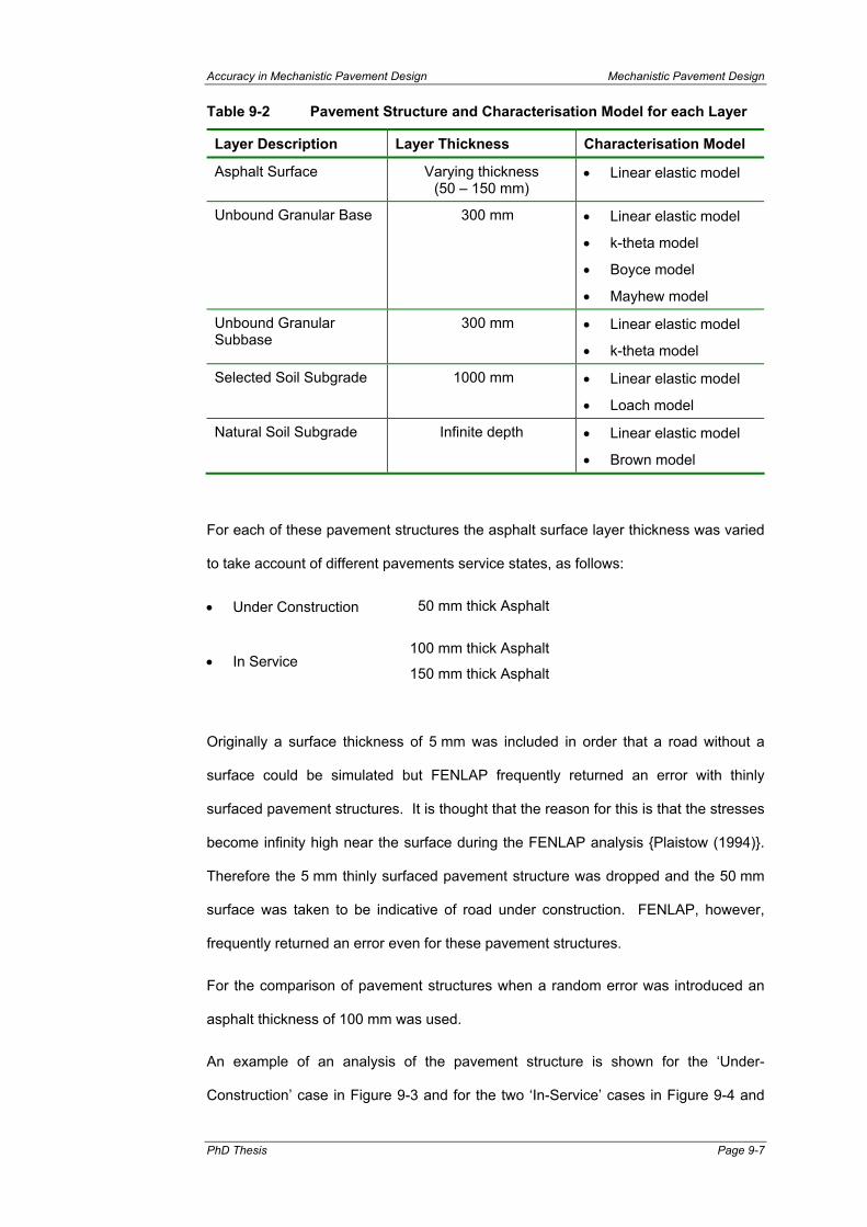
Accuracy in Mechanistic Pavement Design Mechanistic Pavement Design
PhD Thesis Page 9-7
Table 9-2 Pavement Structure and Characterisation Model for each Layer
Layer Description Layer Thickness Characterisation Model
Asphalt Surface Varying thickness (50 – 150 mm)
• Linear elastic model
Unbound Granular Base 300 mm • Linear elastic model
• k-theta model
• Boyce model
• Mayhew model
Unbound Granular Subbase
300 mm • Linear elastic model
• k-theta model
Selected Soil Subgrade 1000 mm • Linear elastic model
• Loach model
Natural Soil Subgrade Infinite depth • Linear elastic model
• Brown model
For each of these pavement structures the asphalt surface layer thickness was varied
to take account of different pavements service states, as follows:
• Under Construction 50 mm thick Asphalt
100 mm thick Asphalt • In Service
150 mm thick Asphalt
Originally a surface thickness of 5 mm was included in order that a road without a
surface could be simulated but FENLAP frequently returned an error with thinly
surfaced pavement structures. It is thought that the reason for this is that the stresses
become infinity high near the surface during the FENLAP analysis {Plaistow (1994)}.
Therefore the 5 mm thinly surfaced pavement structure was dropped and the 50 mm
surface was taken to be indicative of road under construction. FENLAP, however,
frequently returned an error even for these pavement structures.
For the comparison of pavement structures when a random error was introduced an
asphalt thickness of 100 mm was used.
An example of an analysis of the pavement structure is shown for the ‘Under-
Construction’ case in Figure 9-3 and for the two ‘In-Service’ cases in Figure 9-4 and

Mechanistic Pavement Design Accuracy in Mechanistic Pavement Design
Page 9-8 S.D.Gillett
Figure 9-5. It can be seen in these figures that the only difference between each of
these pavement structures is the thickness of the asphalt surface layer.
For each different pavement configuration and circumstances there were a total of five
different analytical runs with varying models and load characteristics as follows:
• Linear elastic model analysis for all layers with dual wheel
loads of 2 x 20 kN each
ELSYM-D
• Linear elastic model analysis for all layers with a single wheel
load of 40 kN
ELSYM-S
• Stress dependent model throughout with k-theta model
describing the base with a single wheel load of 40 kN
Fenlap-K
• Stress dependent model throughout with Boyce model
describing the base with a single wheel load of 40 kN
Fenlap-B
• Stress dependent model throughout with Mayhew model
describing the base with a single wheel load of 40 kN
Fenlap-M
The method used to determine the pavement life from the strain predictions at specific
locations in the pavement structure is that of the SA-MDM as described in an earlier
chapter. The results are, therefore, presented in terms of Equivalent Standard Axles
(ESA) also defined in an earlier chapter and this can be seen on the figures on the
following pages. The critical traffic loading in ESA is shown in red and reproduced at
the bottom of the figure. It can be seen that for the three examples shown the failure
occurs in the surfacing for all three cases, however with the greater thickness of
surface the predicted traffic loading increases as follows:
Asphalt Thickness (mm) Equivalent Standard Axles (ESA)
50 950
100 13,500
150 141,600

Accuracy in Mechanistic Pavement Design Mechanistic Pavement Design
PhD Thesis Page 9-9
Figure 9-3 Mechanistic Analysis of the Pavement Structures Under Construction (50 mm Asphalt Surface)
Pavement Structure - Under Construction (UC):Bituminous prime coat to protect the granular base Unit Weight: 23 kN/m³
Mri= 2,100 MPa ν i= 0.40 Suction: 0 kPaPeak Deflection on the Surface ElsymD ElsymS FenlapK FenlapB FenlapM
δp (mm)= 0.587 0.741 2.855 NS 2.914Strain - Bottom of the Base Layer εx(µε) εy(µε) εz(µε)
Depth= 49 mm ElsymD 266 308 -463ElsymS 273 273 -464
FenlapK 1560 1560 -2160FenlapB NS NS NS
50 FenlapM 1670 1670 -2290Unbound Granular Base Test programme: 2 Lab.: DUT MIG 8
Char.: Mri= 198 MPa ν i= 0.23 Unit Weight: 22 kN/m³k-theta: k1= 1,738 k2= 0.5555 Suction: 0 kPaBoyce: Ka= 1,664 Ga= 27,374 n= 0.4091
Mayhew: Ka= 4,936 Ga= 14,953 n= 0.3597 m= -0.5928 β= -0.8421Stress - Centre of the Base Layer σ1(kPa) σ2(kPa) σ3(kPa) FOS
Depth= 200 mm ElsymD 133 1 -11 14.6ElsymS 201 -11 -11 11.4
FenlapK 166 -14 -15 11.6FenlapB NS NS NS NS
350 FenlapM 84 -21 -23 12.7Unbound Granular Subbase Test programme: 1 Lab.: All MIG 4
Char.: Mri= 235 MPa ν i= 0.28 Unit Weight: 22 kN/m³k-theta: k1= 1,333 k2= 0.6716 Suction: 0 kPa
Stress - Centre of the Base Layer σ1(kPa) σ2(kPa) σ3(kPa) FOSDepth= 500 mm ElsymD 41 -4 -7 19.2
ElsymS 52 -8 -8 15.3FenlapK 83 6 6 16.0FenlapB NS NS NS NS
650 FenlapM 62 6 6 19.6Selected Soil Subgrade Test programme: 1 Lab.: All SFB 1
Char.: Mri= 160 MPa ν i= 0.41 Unit Weight: 16 kN/m³Loach: C= 31,846 D= 0.7333 qf = 1.71 *p + 26 Suction: 3 kPa
Strain - Top of the Selected Subgrade εx(µε) εy(µε) εz(µε)Depth= 651 mm ElsymD -53 -71 131
ElsymS -80 -80 164FenlapK -7 -7 35FenlapB NS NS NS NS
1650 FenlapM -4 -4 28In-Situ Soil Subgrade Foundation Test programme: 1 Lab.: All LOC 2
Char.: Mri= 34 MPa ν i= 0.54 =0.45 Unit Weight: 22 kN/m³
Brown: A= 21,858 B= 0.4820 qf = 0.001 *p + 86 Suction: 32 kPaStrain - Top of the Subgrade Layer εx(µε) εy(µε) εz(µε)
Depth= 1651 mm ElsymD -37 -39 61ElsymS -39 -39 62
FenlapK -12 -12 29FenlapB NS NS NS NS
2650 FenlapM -12 -12 28Minimum Design Loading:
1.582E+062.673E+061.286E+03
50 m
mESA
9.535E+02
2.209E+182.790E+18
1.345E+22
2.362E+22
ESA
4.457E+14
All
- LO
C
Infin
ite
1.858E+21
ESA
3.348E+13
2.005E+22
All
- SFB
1000
mm
All
- MIG
300
mm
300
mm
1.085E+46
1.302E+37
2.825E+40
4.635E+36
Surf
ace
DU
T - M
IG
1.016E+48
3.595E+60
8.088E+49
ESA1.676E+59
9.535E+02
ESA
NS – No Solution

Mechanistic Pavement Design Accuracy in Mechanistic Pavement Design
Page 9-10 S.D.Gillett
Figure 9-4 Mechanistic Analysis of the Pavement Structures In Service (100 mm Asphalt Surface)
Pavement Structure - In-Service (IS):Asphalt Surface and Base Layer Unit Weight: 23 kN/m³
Mri= 2,100 MPa ν i= 0.40 Suction: 0 kPaPeak Deflection on the Surface ElsymD ElsymS FenlapK FenlapB FenlapM
δp (mm)= 0.461 0.567 1.778 1.127 1.482
Strain - Bottom of the Base Layer εx(µε) εy(µε) εz(µε)Depth= 99 mm ElsymD 179 256 -332
ElsymS 290 290 -444FenlapK 913 913 -1230FenlapB 732 732 -965
100 FenlapM 883 883 -1180Unbound Granular Base Test programme: 2 Lab.: DUT MIG 8
Char.: Mri= 198 MPa ν i= 0.23 Unit Weight: 22 kN/m³k-theta: k1= 1,738 k2= 0.5555 Suction: 0 kPaBoyce: Ka= 1,664 Ga= 27,374 n= 0.4091
Mayhew: Ka= 4,936 Ga= 14,953 n= 0.3597 m= -0.5928 β= -0.8421Stress - Centre of the Base Layer σ1 (kPa) σ2 (kPa) σ3 (kPa) FOS
Depth= 250 mm ElsymD 86 -1 -8 17.4ElsymS 123 -9 -9 13.3
FenlapK 69 1 1 20.4FenlapB 47 -16 -17 16.9
400 FenlapM 45 -9 -9 20.3Unbound Granular Subbase Test programme: 1 Lab.: All MIG 4
Char.: Mri= 235 MPa ν i= 0.28 Unit Weight: 22 kN/m³k-theta: k1= 1,333 k2= 0.6716 Suction: 0 kPa
Stress - Centre of the Base Layer σ1(kPa) σ2(kPa) σ3(kPa) FOSDepth= 550 mm ElsymD 32 -5 -7 21.6
ElsymS 39 -7 -7 18.1FenlapK 44 6 6 25.4FenlapB 31 7 7 36.2
700 FenlapM 32 5 5 32.7Selected Soil Subgrade Test programme: 1 Lab.: All SFB 1
Char.: Mri= 160 MPa ν i= 0.41 Unit Weight: 16 kN/m³Loach: C= 31,846 D= 0.7333 qf = 1.71 *p + 26 Suction: 3 kPa
Strain - Top of the Selected Subgrade εx(µε) εy(µε) εz(µε)Depth= 701 mm ElsymD -47 -60 110
ElsymS -66 -66 132FenlapK -1 -1 19FenlapB 1 1 14
1700 FenlapM 1 1 15In-Situ Soil Subgrade Foundation Test programme: 1 Lab.: All LOC 2
Char.: Mri= 34 MPa ν i= 0.54 =0.45 Unit Weight: 22 kN/m³
Brown: A= 21,858 B= 0.4820 qf = 0.001 *p + 86 Suction: 32 kPaStrain - Top of the Subgrade Layer εx(µε) εy(µε) εz(µε)
Depth= 1701 mm ElsymD -34 -36 56ElsymS -36 -36 57
FenlapK -11 -11 26FenlapB -10 -10 24
2700 FenlapM -10 -10 24Minimum Design Loading:
1.337E+23
1.560E+04
2.073E+06
1.275E+231.347E+04
Infin
ite
8.136E+18ESA
5.815E+225.718E+18
All
- LO
C
4.015E+141.552E+24
1000
mm
7.269E+252.589E+25
3.405E+15
All
- SFB ESA
ESA1.302E+54
All
- MIG
300
mm
1.883E+779.526E+108
ESA
4.432E+98
7.148E+624.438E+522.994E+62
2.461E+661.009E+56
3.551E+04
DU
T - M
IG
300
mm
1.508E+42
Surf
ace
100
mm
ESA3.586E+06
1.347E+04
NS – No Solution
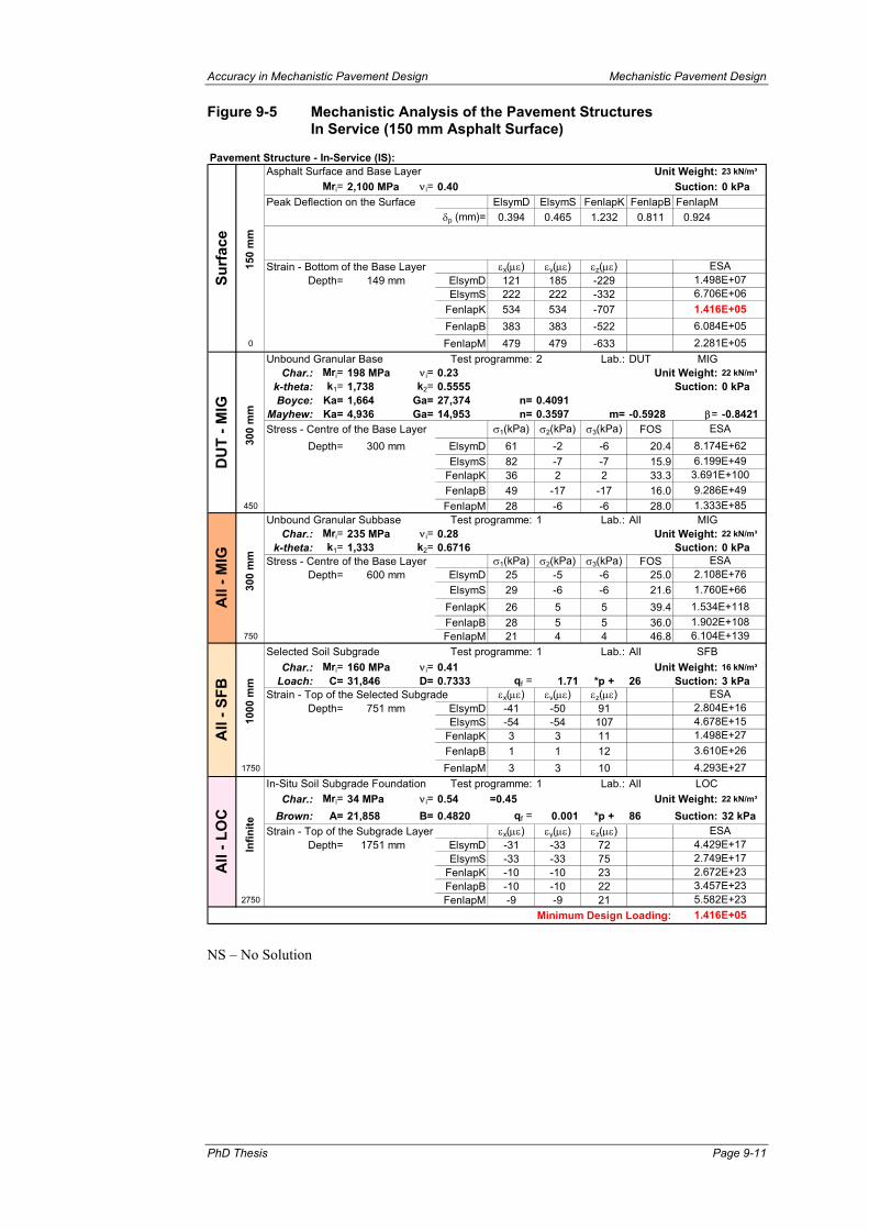
Accuracy in Mechanistic Pavement Design Mechanistic Pavement Design
PhD Thesis Page 9-11
Figure 9-5 Mechanistic Analysis of the Pavement Structures In Service (150 mm Asphalt Surface)
Pavement Structure - In-Service (IS):Asphalt Surface and Base Layer Unit Weight: 23 kN/m³
Mri= 2,100 MPa ν i= 0.40 Suction: 0 kPaPeak Deflection on the Surface ElsymD ElsymS FenlapK FenlapB FenlapM
δp (mm)= 0.394 0.465 1.232 0.811 0.924
Strain - Bottom of the Base Layer εx(µε) εy(µε) εz(µε)Depth= 149 mm ElsymD 121 185 -229
ElsymS 222 222 -332FenlapK 534 534 -707FenlapB 383 383 -522
0 FenlapM 479 479 -633Unbound Granular Base Test programme: 2 Lab.: DUT MIG 8
Char.: Mri= 198 MPa ν i= 0.23 Unit Weight: 22 kN/m³k-theta: k1= 1,738 k2= 0.5555 Suction: 0 kPaBoyce: Ka= 1,664 Ga= 27,374 n= 0.4091
Mayhew: Ka= 4,936 Ga= 14,953 n= 0.3597 m= -0.5928 β= -0.8421Stress - Centre of the Base Layer σ1(kPa) σ2(kPa) σ3(kPa) FOS
Depth= 300 mm ElsymD 61 -2 -6 20.4ElsymS 82 -7 -7 15.9
FenlapK 36 2 2 33.3FenlapB 49 -17 -17 16.0
450 FenlapM 28 -6 -6 28.0Unbound Granular Subbase Test programme: 1 Lab.: All MIG 4
Char.: Mri= 235 MPa ν i= 0.28 Unit Weight: 22 kN/m³k-theta: k1= 1,333 k2= 0.6716 Suction: 0 kPa
Stress - Centre of the Base Layer σ1(kPa) σ2(kPa) σ3(kPa) FOSDepth= 600 mm ElsymD 25 -5 -6 25.0
ElsymS 29 -6 -6 21.6FenlapK 26 5 5 39.4FenlapB 28 5 5 36.0
750 FenlapM 21 4 4 46.8Selected Soil Subgrade Test programme: 1 Lab.: All SFB 1
Char.: Mri= 160 MPa ν i= 0.41 Unit Weight: 16 kN/m³Loach: C= 31,846 D= 0.7333 qf = 1.71 *p + 26 Suction: 3 kPa
Strain - Top of the Selected Subgrade εx(µε) εy(µε) εz(µε)Depth= 751 mm ElsymD -41 -50 91
ElsymS -54 -54 107FenlapK 3 3 11FenlapB 1 1 12
1750 FenlapM 3 3 10In-Situ Soil Subgrade Foundation Test programme: 1 Lab.: All LOC 2
Char.: Mri= 34 MPa ν i= 0.54 =0.45 Unit Weight: 22 kN/m³
Brown: A= 21,858 B= 0.4820 qf = 0.001 *p + 86 Suction: 32 kPaStrain - Top of the Subgrade Layer εx(µε) εy(µε) εz(µε)
Depth= 1751 mm ElsymD -31 -33 72ElsymS -33 -33 75
FenlapK -10 -10 23FenlapB -10 -10 22
2750 FenlapM -9 -9 21Minimum Design Loading:
3.457E+23
6.706E+061.416E+056.084E+052.281E+05
1.416E+05
All
- LO
C
Infin
ite ESA
5.582E+23
2.672E+23
4.429E+172.749E+17
1.498E+27All
- SFB
1000
mm
ESA2.804E+164.678E+15
6.104E+139
ESA8.174E+626.199E+493.691E+1009.286E+491.333E+85
2.108E+76
All
- MIG
1.760E+661.534E+118
300
mm ESA
1.902E+108
4.293E+27
DU
T - M
IG
300
mm
ESA
Surf
ace
150
mm
1.498E+07
3.610E+26
NS – No Solution

Mechanistic Pavement Design Accuracy in Mechanistic Pavement Design
Page 9-12 S.D.Gillett
It may be argued that 950 ESA is unrealistically low but this is a possible failing of the
design method and outside the scope of this work. It does show that the permissible
traffic loading increases with asphalt surface thickness as would be expected.
The mechanistic analyses details for all of the work in this chapter are contained in
Appendix H.
9.3 THE INFLUENCE OF THE MATERIAL VARIATIONS TO PAVEMENT DESIGN
The mechanistic pavement analyses are summarised in Table 9-3, where the different
material combinations for each pavement design are shown. The red text indicates
the layers where the variations were made.
The first and second analyses varied the quality of the base material (Microgranite)
and the subgrade (London Clay) based on the different results obtained from the four
different during Test Programme II. The variation was from the results that predicted
the poorest quality (DUT for Microgranite and LNEC for London Clay) to the best
quality (LRSB for Microgranite and LRCF for London Clay) shown in Table 9-3. The
characteristic resilient modulus values used to rank the materials are shown in Table
9-1.
The second comparison was to take the results of a series of test conducted at a
single laboratory and to investigate the effect of the variation of the results obtained.
Again a pavement structure was selected and first the base material (Hard Limestone)
was varied followed by the subbase material (London Clay). The laboratory tests for
the base material were conducted at LRSB and those of the subgrade at LNEC as
part of Test Programme III. For each of these two materials the range of the test
results obtained at the particular laboratory was divided into 10%ile, 25%’ile, average,
75%’ile and 90%’ile values as shown in Table 9-3. The actual resilient modulus
values resulting from the laboratory tests were shown in the previous chapter.
Considering that each analysis had three different asphalt thicknesses and five
different analytical modelling methods 270 analyse runs were conducted. However,
not all analyses were successful, it was found that FENLAP did not always find a
solution and this is shown in Table 9-4.
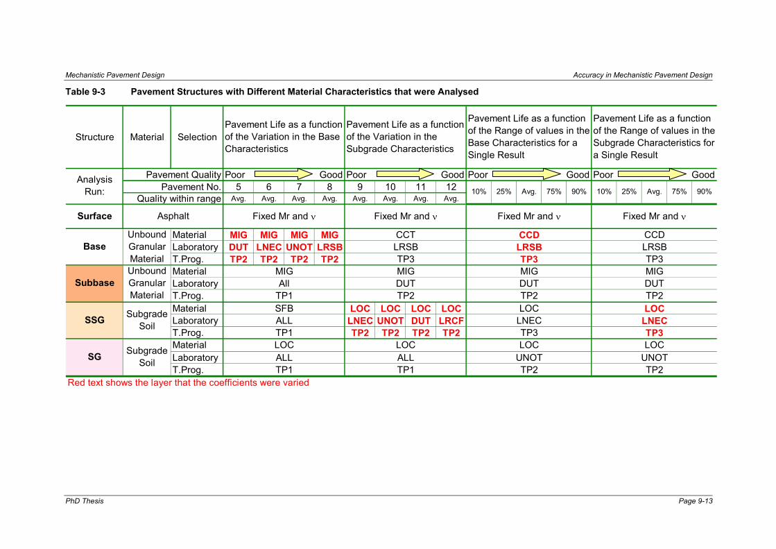
Mechanistic Pavement Design Accuracy in Mechanistic Pavement Design
PhD Thesis Page 9-13
Table 9-3 Pavement Structures with Different Material Characteristics that were Analysed
Structure Material Selection
Pavement Quality Poor Good Poor Good Poor Good Poor GoodPavement No. 5 6 7 8 9 10 11 12
Quality within range Avg. Avg. Avg. Avg. Avg. Avg. Avg. Avg.
Material MIG MIG MIG MIGLaboratory DUT LNEC UNOT LRSBT.Prog. TP2 TP2 TP2 TP2MaterialLaboratoryT.Prog.Material LOC LOC LOC LOCLaboratory LNEC UNOT DUT LRCFT.Prog. TP2 TP2 TP2 TP2MaterialLaboratoryT.Prog.
Red text shows the layer that the coefficients were varied
10% 25% Avg. 75% 90% 10% 25% Avg. 75%
LRSBTP3MIGDUTTP2
LOCALL
Subbase
Asphalt
TP1
Unbound Granular MaterialUnbound Granular Material
Subgrade Soil
MIGAll
TP1
Subgrade Soil
LOCALLTP1
SFBSSG
SG
Fixed Mr and ν Fixed Mr and ν
CCT
ALLTP1
Surface
Base
Fixed Mr and ν
Pavement Life as a function of the Variation in the Subgrade Characteristics
Pavement Life as a function of the Range of values in the Subgrade Characteristics for a Single Result
Fixed Mr and ν
Pavement Life as a function of the Range of values in the Base Characteristics for a Single Result
90%
CCDLRSBTP3
TP2
LOCLNECTP3
TP3
LOCUNOT
MIGDUTTP2
TP2
LOCLNECTP3LOC
UNOT
MIGDUTTP2
CCDLRSB
AnalysisRun:
Pavement Life as a function of the Variation in the Base Characteristics

Mechanistic Pavement Design Accuracy in Mechanistic Pavement Design
S.D.Gillett Page 9-14
Table 9-4 Analyses Conducted showing when Successful Solutions were Achieved
Asph
alt
Thic
knes
s (m
m)
Models
Pav'nt Q'ty Poor Good Poor Good Poor Good Poor GoodPav'nt No. 5 6 7 8 9 10 11 12
Quality Avg. Avg. Avg. Avg. Avg. Avg. Avg. Avg.ELYSM DELSYM SFENLAP KFENLAP BFENLAP MELYSM DELSYM SFENLAP KFENLAP BFENLAP MELYSM DELSYM SFENLAP KFENLAP BFENLAP MELYSM DELSYM SFENLAP KFENLAP B 1 3 3 3 1 1 1 1 1 2 1 2 1FENLAP M 3 3 1 1 1 1 1 1 1 1 1 1Total 1 6 3 6 2 2 1 2 2 3 1 1 2 3 2
AnalysisRun:
Pavement Life as a function of the Variation in the Subgrade Characteristics
Pavement Life as a function of the Range of values in the Base Characteristics for a Single Result
10% 25% Avg. 75% 90%
Pavement Life as a function of the Range of values in the Subgrade Characteristics for a Single Result
Pavement Life as a function of the Variation in the Base Characteristics
50
100
150
Uns
ucce
sful
Run
s
10% 25% Avg. 75% 90%

Accuracy in Mechanistic Pavement Design Mechanistic Pavement Design
PhD Thesis Page 9-15
The results of this table are summarised in Table 9-5, of the 270 analytical runs a total
of 37 (14%) were unsuccessful.
Table 9-5 Summary of the Mechanistic Analysis Run Results
Unsuccessful Runs Analytical Model Name Model Type
No. %
ELSYM – D (Dual Load) Linear Elastic 0 0%
ELSYM – S (Single Load) Linear Elastic 0 0%
FENLAP – K k-theta − model 0 0%
FENLAP – B Boyce - model 21 8%
FENLAP – M Mayhew - model 16 6%
This shows that the more simple linear analysis method is much more likely to provide
an answer to the problem, of course the accuracy of these answers may be
questionable. When FENLAP is used to analyse the pavements absolute success is
found for the more simple k-theta model; the Boyce model yields the worst degree of
success and the Mayhew slightly better than the Boyce model. Of the 37 failures 25
were found on the Under-Construction case (50 mm asphalt surface) while 12 were
for the In-Service case (100 and 150 mm asphalt surface).
A further 40 mechanistic analyses were conducted to investigate the influence of the
introduction of a random error of differing variance as shown in Table 9-6. Since the
material parameters and coefficients were found to vary little (chapter 8) not all of the
analyses were conducted since it was felt that little difference would result. Analytical
runs were conducted for a variance of 0%; 5%; 30% and 50%. As discussed in the
previous chapter two materials were selected for this analysis a granular material –
Hard Limestone and a subgrade soil – London Clay as shown in Table 9-6.

Mechanistic Pavement Design Accuracy in Mechanistic Pavement Design
Page 9-16 S.D.Gillett
Table 9-6 Mechanistic Analysis with Varying Material Characteristics showing Successful Solutions
Structure Material Selection
Variation Quality Little Large Little LargeVariation 0% 2% 5% 10% 30% 50% 0% 2% 5% 10% 30% 50%
MaterialLaboratoryT.Prog.MaterialLaboratoryT.Prog.MaterialLaboratoryT.Prog.MaterialLaboratoryT.Prog.
Red text shows the layer that was varied
SG Subgrade Soil
Surface
Base
Subbase
Unbound Granular Material
Asphalt
LOC
Pavement life as a function of the Range of values in the Base Characteristics when a Random Error is Introduced into the Strain Measurements
SSG
Unbound Granular Material
Subgrade Soil
CCDLRSBTP3
UNOTTP2
MIGDUTTP2
TP3
LOCLNEC
LOCLNECTP3
Pavement life as a function of the Range of values in the Subbase Characteristics when a Randon Error is Introduced into the Strain Measurements
LOCUNOTTP2
MIGDUTTP2
CCDLRSB
AnalysisRun:
TP3
Fixed Mr and νFixed Mr and ν
Of the 40 analytical runs 7 (18%) were unsuccessful, all of those using the Boyce
model, as shown in Table 9-7.
Table 9-7 Mechanistic Analysis with Random Errors Introduced showing Successful Solutions
Asph
alt
Thic
knes
s (m
m)
Mod
els
Var. Q'ty Little Variance Large Variance Little Variance Large VarianceVariation 0% 2% 5% 10% 30% 50% 0% 2% 5% 10% 30% 50%
ELYSM DELSYM SFENLAP KFENLAP BFENLAP MELYSM DELSYM SFENLAP KFENLAP B 1 1 1 1 1 1 1FENLAP MTotal 1 1 1 1 1 1 1
AnalysisRun:
Not
Ana
lyse
d
Not
Ana
lyse
d
Not
Ana
lyse
d
Not
Ana
lyse
d
Pavement life as a function of the Range of values in the Base Characteristics when a Random Error is Introduced into the Strain Measurements
Pavement life as a function of the Range of values in the Subbase Characteristics when a Randon Error is Introduced into the Strain Measurements
Uns
ucce
sful
Run
s
100

Accuracy in Mechanistic Pavement Design Mechanistic Pavement Design
PhD Thesis Page 9-17
9.3.1 Comparison 1 - Variation of the Base Strength from Four Different Laboratories
During Test Programme II, an unbound granular base material (Microgranite) was
tested at four different laboratories. Three test specimens were fabricated to strict
properties, moisture content and density, at each laboratory. Stresses and strains
were measured during the repeated load triaxial test in accordance with a detailed test
procedure and analysed as described. From the analysis material parameters and
coefficients were obtained for the specimens from each laboratory.
A pavement structure was chosen with fixed properties for the surface, subbase and
subgrade layers and the quality of the base varied by the results from each laboratory.
The detailed mechanistic analyses results are contained in Appendix H and tables
containing the predicted traffic life in ESA are shown this appendix. These results are
summarised in Figure 9-6.
As stated in Chapter 2 most common pavement design methods are primarily
concerned with the two critical strain values namely the horizontal tensile strain at the
bottom of the asphalt layer (to limit asphalt fatigue cracking) and the vertical
compressive strain at the top of the subgrade (to prevent excessive permanent
deformation). The SA-MDM method, which is used here, also considers shear
deformation and failure in the unbound granular layers and since this method was
selected for use here, all three criteria are considered. Of course, the lesser ESA
allowed according to each of these three chosen criteria determines the limiting
pavement life. For the pavements chosen here it was found that, almost exclusively,
the pavement life is determined on the basis of asphalt tensile strain, indicating that
fatigue at the bottom of the asphalt layer is the critical failure criterion. However, it is
noted that other failure methods, such as permanent strain in aggregate layers or in
the subgrade, which are not critical for these pavement structures may be critical for
other pavement structures and design methods. Thus the conclusions drawn from this
study might not be universally applicable.
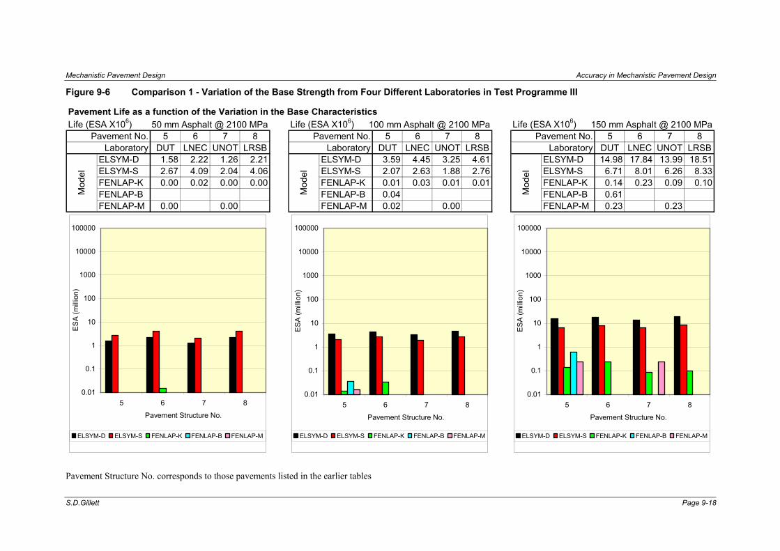
Mechanistic Pavement Design Accuracy in Mechanistic Pavement Design
S.D.Gillett Page 9-18
Figure 9-6 Comparison 1 - Variation of the Base Strength from Four Different Laboratories in Test Programme III
Pavement Life as a function of the Variation in the Base CharacteristicsLife (ESA X106) 50 mm Asphalt @ 2100 MPa Life (ESA X106) 100 mm Asphalt @ 2100 MPa Life (ESA X106) 150 mm Asphalt @ 2100 MPa
5 6 7 8 5 6 7 8 5 6 7 8DUT LNEC UNOT LRSB DUT LNEC UNOT LRSB DUT LNEC UNOT LRSB
ELSYM-D 1.58 2.22 1.26 2.21 ELSYM-D 3.59 4.45 3.25 4.61 ELSYM-D 14.98 17.84 13.99 18.51ELSYM-S 2.67 4.09 2.04 4.06 ELSYM-S 2.07 2.63 1.88 2.76 ELSYM-S 6.71 8.01 6.26 8.33FENLAP-K 0.00 0.02 0.00 0.00 FENLAP-K 0.01 0.03 0.01 0.01 FENLAP-K 0.14 0.23 0.09 0.10FENLAP-B FENLAP-B 0.04 FENLAP-B 0.61FENLAP-M 0.00 0.00 FENLAP-M 0.02 0.00 FENLAP-M 0.23 0.23
Pavement No.
Mod
el
Mod
el
Pavement No. Pavement No.
Mod
el
Laboratory Laboratory Laboratory
0.01
0.1
1
10
100
1000
10000
100000
5 6 7 8
Pavement Structure No.
ES
A (m
illio
n)
ELSYM-D ELSYM-S FENLAP-K FENLAP-B FENLAP-M
0.01
0.1
1
10
100
1000
10000
100000
5 6 7 8
Pavement Structure No.
ES
A (m
illio
n)
ELSYM-D ELSYM-S FENLAP-K FENLAP-B FENLAP-M
0.01
0.1
1
10
100
1000
10000
100000
5 6 7 8
Pavement Structure No.
ES
A (m
illio
n)
ELSYM-D ELSYM-S FENLAP-K FENLAP-B FENLAP-M
Pavement Structure No. corresponds to those pavements listed in the earlier tables

Accuracy in Mechanistic Pavement Design Mechanistic Pavement Design
PhD Thesis Page 9-19
Clearly, the pavement life increases with increasing thickness in the asphalt surface
layer. Taking the FENLAP-K model, for example, the average traffic prediction for the
pavement with 50 mm asphalt is 4,200 ESA, 100 mm is 14,700 ESA and 150 mm is
140,000 ESA all of which are fairly low in terms of pavement life. These are vastly
different, however, from the prediction made by the ELSYM-D model, which predicts
the average traffic prediction for the pavement with 50 mm asphalt is 1.8 x 10⁶ ESA,
100 mm is 4.0 x 10⁶ ESA and 150 mm is 16.3 x 10⁶ ESA, which appear to be much
more realistic estimations.
It is noted that the base is of poor quality (resilient modulus between 198 and
245 MPa) by the standards set in Chapter 2 and this may account for the low
predicted lives. Also, the variation between laboratories is quite small as discussed in
the previous chapter. It is also noted that the third pavement structure (Nos.11; 12; 13
- UNOT) predicts a lower life than the second structure (Nos.8; 9; 10 - LNEC). These
pavements have the same characteristic resilient modulus but the predicted Poisson’s
ratio for the third pavement is greater than that for the second (0.37 against 0.22).
This emphasises the importance of estimating this material parameter accurately
when it is required as an input, i.e. linear elastic and k-theta models in this work.
In summary there is little change in the predicted life from a single pavement structure
with increasing base quality, which implies one of two things, namely:
• The differences in the test results from each of the four laboratories test results is
insignificant with respect to this mechanistic pavement design, or;
• That the modelling process does not provide realistic predictions of material
behaviour which is supported by the vast difference in predictions between the
models, this may be due to the complex nature of these materials in pavement
structures.
Results were not obtained for all of the model types, since many Boyce and Mayhew
models failed to produce a result, for this pavement structure combination.
It is noted that the equivalent dual and single wheel loads (ELSYM) produce varying
results. In general under the single wheel load the life of the pavement is extended for

Mechanistic Pavement Design Accuracy in Mechanistic Pavement Design
Page 9-20 S.D.Gillett
thinly surfaced pavements. This is thought to be due to a concentration of stress
under the dual load at the bottom of the thin surface (which is critical), which would
occur in the centre or upper part (mainly comprehensive zone) of the thicker surfaced
pavements.
For variation in the base quality and the use of different models, the following points
are noted:
• The linear elastic analysis (ELSYM) using the dual and single tyre loads of the
same stress provide similar results;
• The Boyce and Mayhew models are largely unsuccessful when analysing this
pavement structure, however the k-theta model is always successful;
• FENLAP predicts almost immediate failure, particularly for the thinly surfaced
roads, ELSYM predicts almost 100 times the life that FENLAP predicts, clearly
one is incorrect;
• There does not appear to be a trend between the quality of the base in terms of
characteristic resilient modulus and the predicted traffic loading (although there is
only a small change in characteristic resilient modulus).
9.3.2 Comparison 2 - Variation of the Subgrade Strength from Four Different Laboratories
Similarly the comparison was undertaken by applying the variation to a subgrade soil
(London Clay) tested at four different laboratories. Again, three test specimens were
fabricated at each laboratory to the same strict properties. Stresses and strains were
measured and material parameters and coefficients obtained for the specimens from
each laboratory. A pavement structure was chosen whereby the surface, base and
subbase were given common parameters but this time the subgrade was varied with
the results from each laboratory. The actual mechanistic analyses are contained in
Appendix H and tables containing the predicted traffic life in ESA are shown in this
appendix. These results are summarised in Figure 9-7.

Mechanistic Pavement Design Accuracy in Mechanistic Pavement Design
PhD Thesis Page 9-21
Figure 9-7 Comparison 2 - Variation of the Subgrade Strength from Four Different Laboratories
Pavement Life as a function of the Variation in the Subgrade CharacteristicsLife (ESA X106) 50 mm Asphalt @ 2100 MPa Life (ESA X106) 100 mm Asphalt @ 2100 MPa Life (ESA X106) 150 mm Asphalt @ 2100 MPa
9 10 11 12 9 10 11 12 9 10 11 12LNEC UNOT DUT LRCF LNEC UNOT DUT LRCF LNEC UNOT DUT LRCF
ELSYM-D 1533 1009 1013 755 ELSYM-D 187 167 168 156 ELSYM-D 343 330 445 326ELSYM-S 30779 17361 17340 10287 ELSYM-S 159 151 151 142 ELSYM-S 159 158 159 158FENLAP-K 0.03 0.02 0.02 0.01 FENLAP-K 0.03 0.03 0.03 0.03 FENLAP-K 0.25 0.25 0.25 0.25FENLAP-B 53.53 FENLAP-B 0.11 0.02 0.03 0.20 FENLAP-B 0.84 0.33 0.95 0.40FENLAP-M 0.00 0.15 FENLAP-M 0.01 0.02 0.02 0.02 FENLAP-M 0.21 0.25 0.22 0.22
Pavement No.
Mod
el
Mod
el
Pavement No. Pavement No.
Mod
el
Laboratory Laboratory Laboratory
0.01
0.1
1
10
100
1000
10000
100000
9 10 11 12
Pavement Structure No.
ES
A (m
illio
n)
ELSYM-D ELSYM-S FENLAP-K FENLAP-B FENLAP-M
0.01
0.1
1
10
100
1000
10000
100000
9 10 11 12
Pavement Structure No.
ES
A (m
illio
n)
ELSYM-D ELSYM-S FENLAP-K FENLAP-B FENLAP-M
0.01
0.1
1
10
100
1000
10000
100000
9 10 11 12
Pavement Structure No.
ES
A (m
illio
n)
ELSYM-D ELSYM-S FENLAP-K FENLAP-B FENLAP-M
Pavement Structure No. corresponds to those pavements listed in the earlier tables
Mechanistic Pavement Design Accuracy in Mechanistic Pavement Design
Page 9-22 S.D.Gillett
Again there was little change in the predicted life from one pavement structure to
another, although the subgrade material quality is changed quite significantly, by a
factor of 6 (8 to 48 MPa). This may be due to the fact that the influence of the
subgrade layer, being further down in the pavement structure, is less significant than
that for materials that are closer to the surface.
The non-linear FENLAP analyses show an increase of pavement life with increasing
thickness of the asphalt surface layer (with the exception of FENLAP-B - 50 mm
asphalt thickness case) and this is expected. However, the ELSYM linear elastic
analyses show a consistent decrease in predicted life from 50 mm to 100 mm and a
small increase from 100 mm to 150 mm and this is not what one would expect.
Obviously this model is not accurately depicting the real situation since not only is it
expected that longer lives are obtained from thicker asphalt surfaces but also more
realistic results are obtained for thicker asphalt surfaces due to better understanding
of these materials and their behaviour under loading. Thin asphalt layers are more
flexible and, although early cracking may occur, these layers are more able to cope
with higher deflections and thus the life of the pavement structure is greater than if
thicker surfaces were used. This is because stiff layers ‘attract’ higher stresses,
however they distribute them better than thin layers. ELSYM considers each layer as
a continuum in bending and is therefore concerned only with the stress build-up at the
bottom of the layer, however, for thin asphalt layers, shear may be more significant
than tensile strain. Since changes in thickness, when asphalt thickness is small, may
cause large changes in attracted stress as well as large changes in flexibility it is
expected that tensile fibre strain, on which fatigue life is based, would change rapidly.
Therefore, for larger surface thicknesses the flexibility of the layer will drop as the
thickness is increase without much change in attracting stress so extreme fibre strain
will drop and consequently the life will increase.
The FENLAP-B, with 50 mm surfacing, life is anomalous in all aspects (See Figure 9-6
and Figure 9-7) and a computational/ numerical problem seems likely given the non-
convergent solutions of pavements Number 8, 11 and 14 (Figure 9-7).

Accuracy in Mechanistic Pavement Design Mechanistic Pavement Design
PhD Thesis Page 9-23
With respect to the two thicker surfaced pavements, for which all of the analyses were
successful, there is little difference in the predicted lives between the particular
pavement structures with varying subgrade quality. However, there is an enormous
difference between the predictions made by the ELSYM and FENLAP analysis
methods. The average ELSYM life prediction for a pavement with a 100 mm thick
asphalt layer is 160 x 106 ESA as opposed to the 46,000 ESA for the FENLAP and
similarly for the 150 mm thick asphalt surface the ELSYM life prediction is
260 x 106 ESA as opposed to the FENLAP prediction of 370,000 ESA.
A check was conducted on these pavements by plotting the surface deflection bowls
for all models for the two cases (pavement 15 – 100 mm and 16 – 150 mm) as shown
in Figure 9-8 and Figure 9-9. For the 100 mm surface the maximum non-linear
surface deflection was approximately 3 times that for the linearly elastic simulation,
and similarly, for the 150 mm surface pavement, a factor of at least 2 is found.
Deflection bowls have been plotted for all pavement analyses and can be found in
Appendix H. It is thought that the FENLAP analysis does not realise the full potential
of the materials and the predictions are low. Unfortunately, a true deflection bowl was
not measured on a pavement constructed with the relevant structure. Had this been
conducted it would be possible to verify the analytical predictions.
Figure 9-8 Surface Deflection Bowls for a Pavement Structure with a 100 mm Asphalt Surface
0.00
0.20
0.40
0.60
0.80
1.00
1.20
1.40
1.60
1.80
0.0 0.5 1.0 1.5 2.0 2.5 3.0 3.5 4.0 4.5 5.0
Distance from Load (m)
Def
lect
ion
(mm
)
ElsymDElsymSFenlapKFenlapBFenlapM
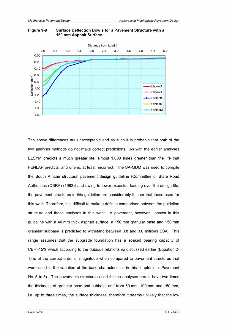
Mechanistic Pavement Design Accuracy in Mechanistic Pavement Design
Page 9-24 S.D.Gillett
Figure 9-9 Surface Deflection Bowls for a Pavement Structure with a 150 mm Asphalt Surface
0.00
0.20
0.40
0.60
0.80
1.00
1.20
1.40
1.60
1.80
0.0 0.5 1.0 1.5 2.0 2.5 3.0 3.5 4.0 4.5 5.0
Distance from Load (m)
Def
lect
ion
(mm
)
ElsymD
ElsymS
FenlapK
FenlapB
FenlapM
The above differences are unacceptable and as such it is probable that both of the
two analysis methods do not make correct predictions. As with the earlier analyses
ELSYM predicts a much greater life, almost 1,000 times greater than the life that
FENLAP predicts, and one is, at least, incorrect. The SA-MDM was used to compile
the South African structural pavement design guideline {Committee of State Road
Authorities (CSRA) (1983)} and owing to lower expected loading over the design life,
the pavement structures in this guideline are considerably thinner that those used for
this work. Therefore, it is difficult to make a definite comparison between the guideline
structure and those analyses in this work. A pavement, however, shown in this
guideline with a 40 mm thick asphalt surface, a 150 mm granular base and 150 mm
granular subbase is predicted to withstand between 0.8 and 3.0 millions ESA. This
range assumes that the subgrade foundation has a soaked bearing capacity of
CBR>15% which according to the dubious relationship discussed earlier (Equation 2-
1) is of the correct order of magnitude when compared to pavement structures that
were used in the variation of the base characteristics in this chapter (i.e. Pavement
No. 5 to 8). The pavements structures used for the analyses herein have two times
the thickness of granular base and subbase and from 50 mm, 100 mm and 150 mm,
i.e. up to three times, the surface thickness, therefore it seems unlikely that the low

Accuracy in Mechanistic Pavement Design Mechanistic Pavement Design
PhD Thesis Page 9-25
predictions made by FENLAP (< 0.1million ESA) are realistic. The ELSYM analysis
predicts pavement lives of the same order for the pavements analysed (1.5 to
4.0 million ESA) which is also low considering the thicker base and subbase. Further,
ELSYM predicts little improvement in the design life with increase in asphalt surface
thickness which also seems incorrect.
It is well established that road construction materials are non-linear inelastic in nature
under loading and therefore the linear elastic methods used in ELSYM are obviously
incorrect since this method treats each layer as a beam and as such allows some
tension (or effective tension) to be present in the analysis. Another possibility is that
FENLAP is basically modelling the situation correctly but that the high strain predicted
is not, in reality, the cause of failure. For example, if the layer is pulling apart, not
bending, it would have a high tensile strain without deflecting in the same manner as
that predicted by ELSYM. Under this scenario the top of the layer might be in tension
too and ELSYM would not predict this. Further, this method does not allow any
change in the material characteristics under loading horizontally and, since it is a
system of definite layers, it assumes a perfect bond between layer interfaces which
may not be correct. An advantage of the linear elastic method is that it has been in
use for a long time, ELSYM since 1963, and is still widely used today. It is
consequently the basis for many established pavement design methods (including the
SA-MDM used here). Therefore, although the modelling method may not be entirely
accurate, the prediction of traffic loading based on these methods has been validated
and subsequently modified over the past years.
The more sophisticated finite element methods and mathematical models used by
FENLAP undoubtedly model the stresses and strains in the material layers better than
the ELSYM approach which, for example, often predicts tension at the bottom of
unbound layers. The finite element approaches, however, lack the wide and long term
use which results in validation against real pavement performance. These approaches
also introduce some artifices in their modelling method, for example, in order to
prevent the occurrence of tension at the bottom of granular materials the following
techniques are used:

Mechanistic Pavement Design Accuracy in Mechanistic Pavement Design
Page 9-26 S.D.Gillett
• It is possible to reduce the stiffness as the compressive stress approaches zero
which will result in very large lateral strains;
• Allow large plastic deformation to occur at the bottom of the layer which will allow
the material to stretch laterally and thus no tension will occur;
• The horizontal stress is increased dramatically at the bottom of the layer in order
to cancel out apparent tension (the technique employed by FENLAP).
This may make the materials and pavements less likely to fail under repeated loading
than is found in practice. Thus neither FENLAP nor ELSYM are likely to provide an
accurate replication of reality. Their different approaches may account for the huge
difference between results from these different methods.
Based on these analyses, using the two analysis methods chosen ELSYM and
FENLAP , the following observations are made:
• The linear elastic analysis (ELSYM) using the dual and single tyre loads of the
same magnitude of stress provide similar results.
• The Boyce and Mayhew models are largely unsuccessful when analysing the
thinly surfaced (50 mm) pavement structure. The k-theta model, however, is
always successful.
• ELSYM predicts a much greater design lives than FENLAP for these roads. The
ELSYM predictions appear to be more realistic.
• There does not appear to be a clear relationship between the quality of the base,
in terms of characteristic resilient modulus, and the predicted traffic loading.
9.3.3 Comparison 3 and 4- Variation of the range of Values of the Base and Subgrade Material Characteristics Conducted at a Single Laboratory
During the analysis and presentation of the material parameters and coefficients in the
previous chapter, it was stated that the 10th and 90th percentile values were calculated
for all values based on the characteristic resilient modulus. For a set of results (CCD
and LOC in Test Programme III) the 25th and 75th percentile results were also
calculated together with the average value (as used in the analyses above). These

Accuracy in Mechanistic Pavement Design Mechanistic Pavement Design
PhD Thesis Page 9-27
values have been applied to two mechanistic analyses, one with varying base
properties and the other varying the subgrade properties. The detailed mechanistic
analyses are contained in Appendix H and tables containing the predicted traffic life in
ESA are shown in this appendix. These results are summarised in Figure 9-10 and
Figure 9-11.
Although the same conclusions with respect to the difference between models apply,
for both analyses, it can clearly be seen that the variation in the base layer has a large
effect on the predicted life of the pavement whereas the variation in the subgrade has
little or no effect. This substantiates the hypothesis that the importance of accurately
determining the properties of the upper layers is greater that that of the lower layers.
Observation made for these comparisons are:
• The linear elastic analysis (ELSYM) using the dual and single tyre loads of the
same stress provide similar results.
• Again ELSYM normally predicts a much greater life for these roads, often 1,000
times the life that FENLAP predicts, and suggestions for this difference have been
given.
• The variation in the base is much more critical than that of the subgrade, as
discussed.

Mechanistic Pavement Design Accuracy in Mechanistic Pavement Design
S.D.Gillett Page 9-28
Figure 9-10 Comparison 3 - Variation within the Range of Values for the Base Strength at a Single Laboratory
Pavement Life as a function of the Range of values in the Base Characteristics for a Single ResultLife (ESA X106) 50 mm Asphalt @ 2100 MPa Life (ESA X106) 100 mm Asphalt @ 2100 MPa Life (ESA X106) 150 mm Asphalt @ 2100 MPa
10% 25% Avg. 75% 90% 10% 25% Avg. 75% 90% 10% 25% Avg. 75% 90%ELSYM-D 38.6 69.1 292 1478 15317 ELSYM-D 25.4 38.1 122.3 313.3 1251 ELSYM-D 73.7 104 302 669 2251ELSYM-S 165 350 1912 21696 1556093 ELSYM-S 15.6 27.6 150.6 504.7 3339 ELSYM-S 0.2 49.6 149 341 1200FENLAP-K 0.03 0.03 0.02 0.02 0.00 FENLAP-K 0.05 0.05 0.05 0.05 0.02 FENLAP-K 0.29 0.31 0.17 0.33 0.21FENLAP-B 1978 177.5 FENLAP-B 0.06 0.38 0.03 0.20 FENLAP-B 0.25 1.04 2.52 0.08 3.44FENLAP-M 0.01 0.01 FENLAP-M 0.03 0.02 0.16 0.23 0.22 FENLAP-M 0.37 0.27 0.25 0.29 1.05
Variation
Mod
el
Mod
el
Variation Variation
Mod
el
0.01
0.1
1
10
100
1000
10000
100000
10% 25% Avg. 75% 90%
Pavement Structure
ES
A (m
illio
n)
ELSYM-D ELSYM-S FENLAP-K FENLAP-B FENLAP-M
0.01
0.1
1
10
100
1000
10000
100000
10% 25% Avg. 75% 90%
Pavement Structure
ES
A (m
illio
n)
ELSYM-D ELSYM-S FENLAP-K FENLAP-B FENLAP-M
0.01
0.1
1
10
100
1000
10000
100000
10% 25% Avg. 75% 90%
Pavement Structure
ES
A (m
illio
n)
ELSYM-D ELSYM-S FENLAP-K FENLAP-B FENLAP-M
Pavement Structure No. corresponds to those pavements listed in the earlier tables

Mechanistic Pavement Design Accuracy in Mechanistic Pavement Design
PhD Thesis Page 9-29
Figure 9-11 Comparison 4 - Variation within the Range of Values for the Subgrade Strength at a Single Laboratory
Pavement Life as a function of the Range of values in the Subgrade Characteristics for a Single ResultLife (ESA X106) 50 mm Asphalt @ 2100 MPa Life (ESA X106) 100 mm Asphalt @ 2100 MPa Life (ESA X106) 150 mm Asphalt @ 2100 MPa
10% 25% Avg. 75% 90% 10% 25% Avg. 75% 90% 10% 25% Avg. 75% 90%ELSYM-D 343 332 292 275 267 ELSYM-D 129 128 122 120 119 ELSYM-D 306 305 302 300 299ELSYM-S 2432 2312 1912 1752 1695 ELSYM-S 153 152 151 150 149 ELSYM-S 150 150 149 149 149FENLAP-K 0.00 0.02 0.02 0.02 0.02 FENLAP-K 0.05 0.05 0.05 0.05 0.05 FENLAP-K 0.34 0.34 0.17 0.34 0.34FENLAP-B 1.17 FENLAP-B 4.09 0.32 0.03 0.17 FENLAP-B 1.34 0.38 2.52 1.80 0.95FENLAP-M FENLAP-M 0.02 0.09 0.16 0.16 0.07 FENLAP-M 0.43 0.36 0.25 0.95 0.54
Variation
Mod
el
Mod
el
Variation Variation
Mod
el
0.01
0.1
1
10
100
1000
10000
100000
10% 25% Avg. 75% 90%
Pavement Structure
ES
A (m
illio
n)
ELSYM-D ELSYM-S FENLAP-K FENLAP-B FENLAP-M
0.01
0.1
1
10
100
1000
10000
100000
10% 25% Avg. 75% 90%
Pavement Structure
ES
A (m
illio
n)
ELSYM-D ELSYM-S FENLAP-K FENLAP-B FENLAP-M
0.01
0.1
1
10
100
1000
10000
100000
10% 25% Avg. 75% 90%
Pavement Structure
ES
A (m
illio
n)
ELSYM-D ELSYM-S FENLAP-K FENLAP-B FENLAP-M
Pavement Structure No. corresponds to those pavements listed in the earlier tables

Mechanistic Pavement Design Accuracy in Mechanistic Pavement Design
Page 9-30 S.D.Gillett
9.3.4 Comparison 5 - Variation with the Introduction of a Random Error into the Strain Measurements
For this sensitivity analysis, a random error was applied to actual strain
measurements for variations ranging from small (2%) to large (50%). The analysis
was conducted and the pavement life predictions made using the mechanistic design
methods. It was found that little variation in the material parameters and coefficients
resulted.
The results of the pavement analyse predicting design life yielded much the same
general trend with respect to the models, as shown in Figure 9-12. Little change in
traffic loading predictions occur between 0% and 50% increase in the magnitude of
the random error. For this analysis it was noticed that, in general, the difference
between predictions made by the different models are not as great as those for
Comparisons 1-4. This substantiates the conclusion from the previous chapter that a
random error in the strain data during the testing procedure has little or no effect on
the final pavement design outcome.
9.4 SUMMARY
The mechanistic design of pavements attempts to model the interaction of various
layers comprising materials in a pavement structure. The South African Mechanistic
Method (SA-MDM) was chosen for use since this method considers failure in unbound
granular base layers.
Numerous mechanistic pavement design analyses were conducted using a linear
elastic method (ELSYM5) and a non-linear method (FENLAP). Both are computer
programs that calculate the stresses and strains at various locations within a
pavement structure under traffic loading.
An 80 kN axle load is simulated by the analysis, however dual wheel loads cannot be
used in FENLAP, therefore a comparison of single and dual loads was conducted
using ELSYM5.

Accuracy in Mechanistic Pavement Design Mechanistic Pavement Design
PhD Thesis Page 9-31
Figure 9-12 Comparison 5 - Variation with the Introduction of a Random Error into the Strain Measurements
Life (ESA X106) 100 mm Asphalt @ 2100 MPa Life (ESA X106) 100 mm Asphalt @ 2100 MPa0% 5% 30% 50% 0% 5% 30% 50%
ELSYM-D 1563 1586 1563 3290 ELSYM-D 1563.07 1585.79 1563.07 3290.25ELSYM-S 407 413 405 1194 ELSYM-S 406.56 412.77 404.51 1193.98FENLAP-K 5809 6201 5809 5206 FENLAP-K 5809.38 6201.12 5809.38 5206.04FENLAP-B FENLAP-BFENLAP-M 6.65 6.15 6.65 951.59 FENLAP-M 6.65 6.15 6.65 951.59
Life (ESA X106) 100 mm Asphalt @ 2100 MPa Life (ESA X106) 100 mm Asphalt @ 2100 MPa0% 5% 30% 50% 0% 5% 30% 50%
ELSYM-D 3290 1557 1549 1642 ELSYM-D 3290.25 1556.66 1549.21 1641.53ELSYM-S 1194 408 409 394 ELSYM-S 1193.98 407.79 409.03 394.08FENLAP-K 5206 5809 1406 786 FENLAP-K 5206.04 5809.38 1406.26 785.54FENLAP-B 0.45 FENLAP-B 0.45FENLAP-M 951.59 6.65 6.65 15.16 FENLAP-M 951.59 6.65 6.65 15.16
Pavement life as a function of the Range of values in the Base Characteristics when a Random Error is Introduced into the Strain Measurements
Pavement life as a function of the Range of values in the Subbase Characteristics when a Randon Error is Introduced into the Strain Measurements
Pavement
Mod
el
Pavement
Mod
el
Variation
Mod
el
Variation
Mod
el
0.01
0.1
1
10
100
1000
10000
0% 5% 30% 50%
ES
A (m
illion
)
ELSYM-D ELSYM-S FENLAP-K FENLAP-B FENLAP-M
0.01
0.1
1
10
100
1000
10000
0% 5% 30% 50%
ES
A (m
illion
)
ELSYM-D ELSYM-S FENLAP-K FENLAP-B FENLAP-M
0.01
0.1
1
10
100
1000
10000
ELSYM-D ELSYM-S FENLAP-K FENLAP-B FENLAP-ME
SA
(mill
ion)
0% 5% 30% 50%
0.01
0.1
1
10
100
1000
10000
ELSYM-D ELSYM-S FENLAP-K FENLAP-B FENLAP-M
ESA
(mill
ion)
0% 5% 30% 50%

Mechanistic Pavement Design Accuracy in Mechanistic Pavement Design
Page 9-32 S.D.Gillett
Some typical values for resilient modulus were quoted in an earlier chapter. In
general good quality crushed rock should have a resilient modulus of between 100
and 600 MPa, whereas a subgrade soil should have a resilient modulus of between
20 and 200 MPa. The results for the three test programmes generally yielded values
within these ranges for the materials tested, although the soils, tested at LNEC, under
Test Programme III resulted in high characteristic resilient moduli.
Five comparisons were made by varying material properties and conducting
mechanistic pavement analyses to determine the pavement life in ESA. The main
conclusions from these comparisons are:
• Pavement life increases with asphalt thickness for thick surfaces (100 mm and
150 mm) for the same pavement structure and material characteristics. For thin
surfaces (50 mm), however, when analysed using linearly elastic models the
pavement life often exceeds that of identical pavements with thicker surface
layers. This can be explained by the fact that the linear elastic analyses assume
that thinner surface layers are more flexible and thus able to withstand higher
deflections, stresses, without significant failure.
• Vastly different predictions of life were calculated by the linear elastic models to
those of the non-linear methods. This worrying revelation indicates that one of the
methods is not modelling the pavement correctly. This is substantiated by the fact
that predicted surface deflection bowls showed large deflection variations
between linear elastic and non-linear modelling methods.
• Dual loads were found to cause more damage to thinly surfaced roads than
equivalent single loads. This is due to the coincidence of stresses, thus increases
in stress magnitude, at the bottom of the thin surface, which is the critical area, for
dual wheel loads. This concentration of stress occurs in the centre or upper part
of the thicker surface pavements, an area that is less critical.
• Variations in the base quality (198 to 245 MPa) had little effect on the predicted
life, thus the results from the four laboratories in Test Programme II resulted in
similar pavement design predictions. This is substantiated by the fact that when a

Accuracy in Mechanistic Pavement Design Mechanistic Pavement Design
PhD Thesis Page 9-33
greater range of base material properties were compared against one another the
effect on the pavement life was much greater.
• Variations in the subgrade quality (8 to 48 MPa) also had little effect on the
predicted life of the pavement. However the variation of this material was much
greater (6 times) and therefore it is surmised that this layer has much less
influence on the design life of the pavement, at least when tensile asphalt strain is
the parameter controlling pavement life. This is substantiated by the outcome of
the sensitivity analysis which concluded that there was little change in design life
with large variation in the material properties of the subgrade layer.
• Poisson’s ratio values, where required, have a marked effect on the modelled
pavement life predictions and care must be taken to estimate this parameter
correctly.
• During the non-linear modelling analysis the complex Boyce and Mayhew models
often fail to produce a result, particularly when the surface layer was thin (50 mm).
Conversely the k-theta model proved to be very robust as were the linear elastic
analyses.
• Large variations to the random errors in strain measurements at the testing level
had very little effect on the ultimate predicted life of the pavement. This implies
that the material models at all levels are able to cope with large variations in the
basic data used to predict the material properties over a large range of stress
paths.


Accuracy in Mechanistic Pavement Design Summary and Conclusions
PhD Thesis Page 10-1
10 SUMMARY AND CONCLUSIONS
10.1 SUMMARY
All of the laboratory work and much of the analysis reported in this thesis was
conducted while the author was employed as a research assistant to work on the
‘Science Project’ between 1990 and 1993. During this period he was based in Lisbon,
Portugal.
The author visited all of the participating laboratories and conducted substantial
repeated load triaxial tests, comprising five test programmes at LNEC, UNOT and
LRSB using the repeated load triaxial apparatus of various configurations, and varying
instrumentation, to measure the deformation of the specimens under loading. He was
particularly involved with the development of the ‘String of Wheels’ for the
measurement of radial deformation of specimens.
This work uses the data obtained during these test programmes to identify and
quantify errors involved in unbound material testing (subgrade soils and granular
materials) and goes some way to identifying the consequence of these errors on the
final pavement design.
A number of materials, that are indicative of road construction materials across
Europe, were selected and tested and the results have been analysed. These
materials comprised both subgrade soils, which are used in road foundations, as well
as unbound granular materials that are used in the upper layers (subbase and base).
An artificial material was also tested in order that comparisons could be made
between repeated load triaxial apparatus, and the various instrumentations,
independently of the material characteristics.
As a result of the detailed instrumentation comparison in this work the magnitude of
potential errors are quantified and certain recommendations are presented and
conclusions made.
The objective of repeated load triaxial testing is to produce material parameters that
characterise the materials, such as resilient modulus and Poisson’s ratio. However, it

Summary and Conclusions Accuracy in Mechanistic Pavement Design
Page 10-2 S.D.Gillett
is recognised that these road construction materials are heavily stress dependent and
therefore a single value of these parameters to describe a material is inadequate.
Nonetheless, common analytical methods used for practical pavement design require
such single material parameters. Furthermore, engineers favour assigning values to
materials so that they can easily rank various material and pavement quality options.
It is with this in mind that the author has chosen a particular stress level to define the
quality of materials rather than using some arbitrary stress level, for example that of
Paute et al (1986). He has determined a ‘reasonable’ stress level as applied to the
base and the subgrade of a ‘reasonable’ pavement structure under ‘reasonable’ traffic
loading and defined this as the ‘characteristic stress’. Analytical analysis, using
mathematical models and applying characteristic stress value results, were
undertaken to obtain characteristic material parameters (resilient modulus, Poisson’s
ratio, volumetric and shear strain). A simple iterative analysis shows that the
characteristic stresses are insensitive to the change in the initial assumed material
parameters. Although this definition of characteristic stress remains open to some
criticism, it does result in a numeric parameter with which comparisons of materials
and, indeed, pavements comprising these materials can be made.
The repeated load triaxial test data has been analysed using seven previously
published material models. These models attempt to describe the behaviour of road
construction materials under traffic loading, and all require material coefficients that
are established for the particular material. These coefficients have been established
from repeated load triaxial testing.
Two different numerical analysis methods were used to determine the model
coefficients for these models and various materials. The choice of the method was
dependent on the complexity of the model being considered. A range of pavement
structures of ‘reasonable’ layer thicknesses comprising the material parameters, as
characterised by the material testing programme, were analysed.
The stresses and strains obtained from the analytical methods were then applied to
the South African mechanistic design method, which was selected as a suitable
pavement design method, enabling the pavement life for each different pavement
Accuracy in Mechanistic Pavement Design Summary and Conclusions
PhD Thesis Page 10-3
structure to be established. This allowed the author to make comparisons of the
different analytical methods and material models.
10.2 DISCUSSION
Apparatus and Instrumentation
Of the eight repeated load triaxial apparatus contained in five laboratories, considered
in this work, seven vary to some degree. Importantly, there is a high variability
between the instrumentation, which measures stresses and strains.
There is no system that clearly stands out above other systems as giving improved
performance. Indeed most systems have been developed because of certain needs
or preferences within the particular laboratory. They all use some form of electronic
transducer, or strain gauge, to measure the movements and stresses and capture the
data using an electronic device.
During this work, some basic guidelines have been established with respect to
repeated load triaxial testing of subgrade soils and unbound granular materials in the
apparatus as follows:
a) The axial load cell should be placed on the loading rod inside the cell in
order to avoid the effects of friction between the rod and the cell.
b) Variable confining pressure repeated load triaxial apparatus are desirable
but require a cell surrounding the specimen. This makes accessing the
instruments during a test difficult.
c) Constant confining pressure repeated load triaxial apparatus are generally
used for large specimens (for testing large particle material such as
granular subbase and base materials) and instead of a surrounding cell an
internal vacuum is used. Unfortunately, with these apparatuses the
confining pressure cannot be varied but the instrumentation can be easily
accessed. Also, larger specimens require more material, are more time
consuming to fabricate, are more difficult to manoeuvre and the repeated
load triaxial apparatus required to test them is much larger and thus, more
expensive.

Summary and Conclusions Accuracy in Mechanistic Pavement Design
Page 10-4 S.D.Gillett
Sample instrumentation may be fixed to the specimens by a number of different
methods. Placing measurement studs or pins into the specimen provides a positive
method of measurement of axial specimen deflection, which eliminates the possibility
of slip, which could conceivably occur between a spring-loaded clamp and the
membrane. The major drawback associated with using studs or pins in a granular
material is that specimen preparation is greatly complicated because of the presence
of a stud (or pin), which protrudes both into and out of the specimen. This is of
greater significance during the preparation of a granular specimen, since studs must
be affixed to the mould during specimen compaction, which can cause problems with
the material density around the studs.
a) Axial deformations measured from the top platen give erroneous results
due to end effects between the specimen and the platens. Measurement
should be taken some distance from the end platens. Commonly this is
conducted between one third and two thirds of specimen height or between
quarter points. The greater gauge length obtained from quarter points does
result in larger deformations, which will result in a more reliably measured
strain reading. Three measuring points should be positioned at 120° to one
another around the specimen, in order that any discrepancies such as tilting
can be detected. However, the laboratories assessed in this work have not
always been found to be practical due to extra instrumentation
requirements and space within the cell.
b) Similarly, radial measurement should be taken within the third or quarter
height of the specimen, to eliminate the end effects. As with axial
deformation measurement, instruments should be positioned at 120° to one
another but, again, this has not always been found to be practical.
c) Some axial measuring LVDTs are glued onto the membrane, which
surrounds the specimen, while others are attached to studs embedded into
the specimen, penetrating the membrane. These two methods of
instrumentation attachment did not show great discrepancies with each
other. However, care should be taken if radial measuring apparatuses are

Accuracy in Mechanistic Pavement Design Summary and Conclusions
PhD Thesis Page 10-5
glued onto the membrane because the changing of pressure, in the cell or
within the specimen, may cause membrane compression and consequent
misreading of radial strain.
An experiment with an artificial specimen tested at each of the laboratories, and at
one laboratory with multiple instrumentation, has given some confidence that different
instrumentation systems can give similar, although not identical, results.
Measurements with instrument influenced variability in the ranges of ±5 to ±10% of the
mean strain value should be expected.
These artificial specimen tests could not use embedded fixings and did not use glue-
on fixings. Embedded fixings cause some disturbance to the specimen and this is
thought to be a further contributor to differences between instrument outputs, although
this could not be assessed completely independently of other variables. For many
purposes embedded fixings are preferred, as they avoid membrane interaction
problems.
It is very important that some understanding of the possible errors and inaccuracies of
the particular system is undertaken by monitoring and calibration. An example of this
is shown by the fact that digital noise was found to account for strain measurements of
up to 90µε during this study.
It is therefore concluded that laboratories should conduct an assessment of their
instrumentation and define the error for each instrument. It may be possible to
periodically check the entire test apparatus and instruments using an artificial
specimen of known mechanical properties as a reference.
It has been shown that the mean radial measurement for testing three specimens
each manufactured and tested at four laboratories is -140 µε, the standard deviation is
68 µε and the coefficient of variation is 49%, which is a great deal poorer than the
12% value of the axial resilient strain measured between the laboratories. It is thus
concluded that there are greater errors in the radial measurement systems than the
axial measuring systems.

Summary and Conclusions Accuracy in Mechanistic Pavement Design
Page 10-6 S.D.Gillett
For the unbound granular material, the axial resilient strain results show little
systematic difference, although improved readings appear to result from a larger
specimen size. The variability in readings is particularly high for the UNOT tests
(which may be due to stud rotation generating apparent strain - sometimes increasing,
sometimes decreasing the measured values above the average obtained at all the
laboratories). For radial resilient strains all laboratories yielded a large scatter in
strain values. There was no systematic variation in radial strains between
laboratories.
Tests conducted on the artificial specimen shows that there is a substantial variation
in the loads (stresses) applied to the specimens and this will have an obvious effect
on the strains. It is, therefore, necessary to take actual stress values into
consideration when comparing and analysing results rather than to simply assume
that the stress levels specified were achieved.
Despite the advice offered here, it is clear that the ‘best’ performance will still contain
many uncertainties and inexactitudes that are due to a whole range of factors. The
value of inter-laboratory comparisons of the type recorded here is high. Systematic
errors were highlighted, procedures crosschecked and quality generally improved.
Compaction Methods
It was found during this study that large differences in the test results occurred when
identical materials were tested at different laboratories.
a) These different results were shown to be due to differences in the
compaction method used by the laboratories, rather than the apparatus and
instrumentation used to capture the data.
b) Methods of compaction which induce high levels of shear, such as the
vibrating hammer (LNEC) and manual tamping under cyclic preloading
(DUT) result in lower permanent strains than the methods where the
compaction is full face, inducing less shear, such as the ‘vibrocompression’
apparatus (LRSB) and vibrating table and full face static load (UNOT).
Thus, the method of compaction is an important factor in attaining
Accuracy in Mechanistic Pavement Design Summary and Conclusions
PhD Thesis Page 10-7
consistent results between repeated load triaxial tests. Therefore, it is
imperative that a standardised method of specimen manufacture and
compaction is established between laboratories if the results obtained from
testing are to be compared and applied to a single pavement design
method.
Removal of ‘Poor’ Data
The author has devised and described a method for removing outliers from the test
data based on the difference between the modelled and experimental material
parameters for each stress path applied to a particular specimen. After considering a
number of degrees of data exclusion it is concluded that, in general, for the test
procedures used (stress paths applied), better correlation between the modelled and
experimental data is obtained when the ‘worst’ 10% of the data is removed.
Critical Locations in a Pavement Structure Associated with Failure
Most pavement design procedures are primarily concerned with the two critical strains
values namely the:
a) Horizontal tensile strain at the bottom of the asphalt layer (to limit asphalt
fatigue cracking), and;
b) Vertical compressive strain at the top of the subgrade (to prevent excessive
permanent deformation).
Of the methods reviewed herein, only the South African design method presented a
means of assessing the shear deformation and failure in the unbound granular layers
for subbases and bases in pavements. However, the shear deformation and failure in
the unbound granular layers for subbases and bases in pavements was not found to
be critical for the pavement structures considered herein and it is therefore concluded
that the two criteria, above, are satisfactory.
Introduction of a Random Error to Test Data
The introduction of a random error at different variations (up to 50% of the
measurement) was found not to affect the final outcome of the analyses when the
variation was below 30% but to rapidly increase once 30% was exceeded. This has
an important consequence for the accuracy at instrumentation level. It implies that

Summary and Conclusions Accuracy in Mechanistic Pavement Design
Page 10-8 S.D.Gillett
some variations found in measurements using electronic instrumentation, such as
random electronic noise, may not be as important as the inaccuracies generated by
other aspects of the testing, such as specimen manufacture.
Comparison of the Test Results from the Test Programmes
This work investigated the effect that using two different methods of analysis have on
the resultant characteristic material parameters using a single set of test results. SFB,
which for this work is defined as dry single sized sand, is considered to behave as a
subgrade soil as well as an unbound granular material under loading. Therefore, the
two methods of analysis, used in this work, were applied i.e. the behaviour can be
modelled as subgrade soil and as an unbound granular material. This means that all
seven of the material models considered in this work could realistically be applied to
the same set of SFB test results obtained from each laboratory.
a) It was concluded that there is greater variation between the resilient moduli
as predicted from analysing the results from a single specimen (from one
laboratory) using different models than there is when the results from
different specimens are analysed using a single model. Therefore it seems
more important to select an appropriate predictive model and analytical
method than is it to obtain test results which are ‘close’ to each other.
b) An investigation was conducted regarding the effect that the variation of the
testing of a granular base material at four different laboratories made on the
pavements’ life. It was found that very little variation in the pavements life
results from using the material parameters from the various laboratories. It
was noted that the actual results from the laboratories were close to one
another.
c) Similarly, a study of the effect on the pavement’s life with the variation of
testing a fine-grained subgrade soil at four different laboratories concluded
that although the test results from the laboratories were quite varied, the
different material parameters made an insignificant amount of difference to
the predicted pavement life.

Accuracy in Mechanistic Pavement Design Summary and Conclusions
PhD Thesis Page 10-9
d) An investigation was also conducted regarding the effect on the pavement’s
life due to the variation of the results when testing a granular material (base
or subbase) at a single laboratory. It was found that a considerable
difference was found in the predicted life of the pavement when the more
simple linear elastic analysis is conducted using the material parameters
obtained, whereas very little variation in pavement life was found for the
more complex non-linear method. It must be noted that the actual variation
between the results from tests of different specimens at a single laboratory
was found to be considerable.
e) Similarly, a study was undertaken as to the effect on pavement life caused
by the variation of the results obtained from testing the fine-grained
subgrade soil at a single laboratory. It was found that very little difference
was found in pavement life even though the variation in the results obtained
is considerable.
Based on the above five points it is concluded that it is not as important to conduct
detailed, and expensive, testing and analyses on materials that are to be used in the
lower foundation layers of a pavement (subgrade soils) as it is on the upper granular
layers (subbase and base).
These studies show that not only are there significant differences between the results
obtained from specimens tested at different laboratories but also between specimens
tested at a single laboratory. Most of the laboratories were not conducting regular test
programmes using these apparatus, and the fact that procedures were not as refined
or efficient as they might be may go someway to explaining this. With the introduction
of standard specifications for repeated load triaxial testing of road construction
materials efficiency and repeatability should improve with time and familiarity.
Comparison of Pavement Structure Incorporating the Material Parameters
Five comparisons were made by varying material properties of different pavement
structures and conducting a mechanistic pavement analysis to determine the
pavement life (ESA) based on a common method. The main conclusions from these
comparisons are:

Summary and Conclusions Accuracy in Mechanistic Pavement Design
Page 10-10 S.D.Gillett
a) Pavement life increases with asphalt thickness for thick surfaces (100 mm
and 150 mm) for the same pavement structure and material characteristics.
For thin surfaces (50 mm), however, when analysed using linearly elastic
models, the pavement life often exceeds that of identical pavements with
thicker surface layers. This can be explained by the fact that linear elastic
analyses, when horizontal asphalt tensile strain is critical, compute small
strains in thinner surface layers due to their greater flexibility. Thus the
layer is able to withstand a greater number of load applications before
failing.
b) Dual wheel loads were found to cause more damage to thinly surfaced
roads than equivalent single loads. This is due to the coincidence of
stresses at the bottom of the thin surface, which is the critical area, for dual
wheel loads. This concentration of stress occurs in the centre or upper part
of the thicker surface pavements, an area that is often considered less
critical than the bottom of these layers, for example.
c) The linear elastic layered analyses predict very different pavement lives to
those of the non-linear finite element methods. The reason for this has not
been fully determined but seems to indicate that at least one of the methods
is not modelling the pavement correctly. This is substantiated by the fact
that predicted surface deflection bowls showed large deflection variations
between linear elastic and non-linear modelling methods. It is known that
ELSYM5 does not correctly calculate stresses and strains for unbound
materials (i.e. it allows tension). This method, however, has benefited from
long term use and substantial field verification and would appear to predict
more reasonable pavement lives. The FENLAP analytical method would
benefit from full-scale validation in order to establish whether the low
predictions are realistic and if not, what factors should be included in the
computations which are currently ignored.
d) Variations in the base quality (characteristic resilient modulus between 198
and 245 MPa) had little effect on the predicted life, thus the results from the

Accuracy in Mechanistic Pavement Design Summary and Conclusions
PhD Thesis Page 10-11
four laboratories in Test Programme II resulted in similar pavement design
predictions. This is substantiated by the fact that when a greater range of
base material properties were compared against one another (in
Programme I) the effect on the pavement life was much greater.
e) Variations in the subgrade quality (characteristic resilient modulus between
8 and 48 MPa) also had little effect on the predicted life of the pavement.
However the variation of this material was much greater (6 times) and
therefore it is concluded that this layer has much less influence on the
design life of the pavement. This is substantiated by the outcome of the
sensitivity analysis which concluded that there was little change in design
life with large variation in the material properties of the subgrade layer.
f) Poisson’s ratio values, where required, have a marked effect on the
modelled pavement life predictions and care must be taken to estimate this
parameter correctly.
g) During the non-linear modelling analysis the complex Boyce and Mayhew
models often fail to produce a result, particularly when the surface layer
was thin (50 mm). Conversely the k-theta model proved to be very
analytically robust as were the linear elastic analyses.
h) Large variations (random errors) in strain measurements at the testing level
had very little effect on the ultimate predicted life of the pavement. This
implies that the material models at all levels are able to cope with large
variations in the basic data used to predict the material properties over a
large range of stress paths.

Summary and Conclusions Accuracy in Mechanistic Pavement Design
Page 10-12 S.D.Gillett
10.3 CONCLUSIONS
The overall conclusions that were obtained from the triaxial testing of road
construction materials and the subsequent analysis of the results as described in this
thesis are that:
a) Although the resilient modulus characteristics for the subgrade soils from
the different laboratories varied by a factor of 6, applying these different
material parameters to pavement designs made an insignificant amount of
difference to the predicted pavement lives. It is therefore concluded that
sophisticated and expensive repeated load triaxial testing of materials in the
lower layers (subgrade soils) is not beneficial as far as pavement analysis
is concerned, because, for most pavements used here the wide soil
variability has little effect on pavement life. Less complex laboratory tests
might, therefore, be employed for testing subgrade soils and, similarly, the
analysis of their results to produce the material characterisation can be
simple without loss of relevant pavement design precision.
b) The range of the experimental resilient modulus values for the soils was
found to be somewhat less than the range of the values estimated by the
models for these materials. However the range of the experimental values
for the unbound granular materials was found to be approximately equal to
the modelled values. This implies that it is not as important to use
sophisticated models for lower layers (subgrade soils) as it is for the upper
layers in a pavement, where unbound granular materials are commonly
used. Hence, this supplies a second reason for giving more attention to the
characterisation of the material in the upper layers (UGM) than to the
characterisation of lower layers (soils).
c) Random instrumentation errors in the range ±30% are less concerning than
small bias errors as the implicit averaging process which occurs when fitting
a material model to the collected readings, minimises their impact on the
ultimate computed pavement life. Therefore during the examination of test

Accuracy in Mechanistic Pavement Design Summary and Conclusions
PhD Thesis Page 10-13
data more effort should be given to identifying, and removing, systematic
(bias) errors rather than scatter (noise) errors.
d) There is a major effect on predicted pavement life depending on the
particular selected analytical method. It is suggested that only analytical
techniques for which performance criteria have been developed and
validated, preferable against full scale trials, are useful.
e) Generally, simpler constitutive relationships give acceptable fits to
laboratory data. Given the difficulties in applying complex models and the
uncertainties and errors experienced elsewhere it is recommended that
these simpler models are normally used.
f) It has been observed that the computed life, and hence design thickness, of
a pavement is much more sensitive to the material model used to describe
the behaviour of the laboratory soil or aggregate specimen under loading
and to the analytical pavement method (ELSYM or FENLAP) than it is to
any variations in material behaviour likely to be observed with or between
laboratories. In the light of the previous conclusions it is, therefore,
concluded that the greatest care should be taken to select the most
appropriate analytical procedure.
In addition to these, useful conclusions obtained from this work are:
• Variability of strain readings in the range ±5 to ±10% of the mean strain
value should be expected from on-sample instrumentation.
• Greater error magnitudes (approximately 4 times) occur with the radial
measurement systems than with the axial measuring systems.
• Different results from different laboratories were shown to be due, largely,
to differences in the compaction method used by the laboratories rather
than the apparatus and instrumentation used to test the specimen and
capture the data.

Summary and Conclusions Accuracy in Mechanistic Pavement Design
Page 10-14 S.D.Gillett
• Better correlation was found between the modelled and experimental
data when the ‘worst’ 10% of the data is removed. Therefore the removal
of 10% of ‘outliers’ using the method described herein, is recommended
in future.
• Poisson’s ratio values, where required, have a marked effect on the
modelled pavement life predictions and care must be taken to estimate or
measure this parameter correctly.
• Pavement life predictions are much more sensitive to variations in soil
and aggregate characterisation when using a linear elastic layered
analysis (ELSYM) than when using a finite element method (FENLAP).
Is it noted that the older linear elastic approach has benefited from field
validation and therefore given (d), above, calibrating the pavement life
predictions of the newer finite element methods directly to observed
performance should improve the practical application and usefulness of
these methods.
• Test repeatability was found to be poor with a coefficient of variation
about the mean for soils having a typical range of ±80% and up to ±170%
for UGM. Together with conclusions (a) and (b), above, better predicted
pavement lives/ thicknesses would be obtained if more accurate test
results were obtained during testing of UGM. However, the coefficient of
variation about the mean for models is considerably better with a typical
value of ±20% for soils and ±40% for UGM. This implies that the
predicted designs for soils based on existing tests methods and
modelling methods are satisfactory but that, better predicted answers
would be obtained if more accurate test results were obtained during
testing of UGM although the models mask this inaccuracy somewhat.

Accuracy in Mechanistic Pavement Design Summary and Conclusions
PhD Thesis Page 10-15
10.4 RECOMMENDATIONS FOR FUTURE WORK
Specimen Manufacture
A detailed investigation should be conducted on the various methods of specimen
manufacture and, importantly, compaction. Based on the conclusions above it is
apparent that a uniform method of specimen manufacture is required. This work
should aim to draw up a detailed testing specification with the compaction and
specimen manufacture for various road construction materials. It is recommended
that a compaction standard be formulated that does not just consider the ease of
‘producing’ specimens in the laboratory but also a procedure that manufactures
specimens that closely replicate the in-situ conditions.
Instrumentation Advances
Since the laboratory testing was conducted for this work (1990 to 1993) less
expensive, commercially available, instrumentation with much improved accuracy is
certainly available. This is particularly desirable for radial measuring instrumentation
which was shown to be less accurate than the instrumentation methods that measure
axial strain. This instrumentation will improve the ease with which these sophisticated
laboratory tests might be conducted. Advances in this instrumentation, as well as the
entire apparatus within which the specimen is tested and the method by which they
are employed, should be continually monitored.
Characteristic Values
It is recommended that further work be undertaken in deriving acceptable
‘characteristic’ values. These should not just be the stress values for materials based
on the expected depth in the pavement of these materials but also the predicted
acceptable material parameters, for example resilient modulus and Poisson’s ratio. If
acceptable models were defined for material this could be extended to defining
acceptable characteristic model coefficient values as well.
Analytical Modelling
Numerous analyses were conducted for a range of road construction materials
resulting in the material properties (material parameters and model coefficients) being
produced for certain analytical models. During this work some problems in
determining realistic solutions to some models was encountered and a pragmatic set

Summary and Conclusions Accuracy in Mechanistic Pavement Design
Page 10-16 S.D.Gillett
of rules (minimum and maximum values for the coefficients and parameters) was
formulated. This allowed for the characterisation of ‘good’ and ‘bad’ results, where the
bad results were unrealistic and could be removed. Future work might be to refine
these rules with respect to the behaviour of road construction materials.
The mathematical models used in this work fall short of perfectly predicting the
behaviour of the materials under repeated loading. Although perfectly correct
modelling may never be achieved, largely due to the fact that repeated load triaxial
testing does not correctly simulate the true pavement situation, with the increase in
capabilities of computing methods models should be continually improved.
Analytical Pavement Design Methods
Substantial differences in the predicted life for the same pavement structure resulted
from the two analytical methods used to determine the stresses and strains at certain
critical points in the pavement structures. ELYSM5 predicts that the structure will
carry substantially more traffic than the predictions made by FENLAP. It is known that
ELSYM5 does not correctly calculate stresses and strains for unbound materials (i.e. it
allows tension). This method, however, has benefited from long term use and
substantial field verification. The FENLAP analytical method would benefit from full-
scale validation in order to establish whether the low predictions are realistic. If a
reliable source of field data could be obtained (for example that of the HVS in South
Africa) then these methods (and others that are available) and their respective
predictions regarding the actual field occurrences could be compared to one another.
Standard Specifications
The Science Project has resulted in the formulation of a standard specification for
repeated load triaxial testing of subgrade soils and unbound granular materials which
has formed the basis of a new CEN standard to be implemented across Europe
CEN (2000). Similarly a standard specification is being applied in the USA, Australia
and probably other countries. Future work might investigate the success or otherwise
of the implementations of these specifications worldwide and make recommendations
for improvement based on the past decade’s experience. Importantly, this should be
applied from the specimen manufacture stage through to the pavement design phase.

Accuracy in Mechanistic Pavement Design Summary and Conclusions
PhD Thesis Page 10-17
The use of an artificial specimen resulted in some important findings in this work. This
could be extended to making firm recommendations as to the composition of such a
material and its use for calibration of repeated load triaxial apparatus worldwide. A
database of the results from instrumentation and apparatus calibration would benefit
all users.
Acceptable Errors
During this work the errors that occur during repeated load triaxial testing and the
subsequent analysis of the test results resulted in some revelations, for example, the
introduction of a random error at different variations had little affect on the final
outcome of the analyses. It is recommended that all future work consider the potential
errors in testing and analysis and then clearly define such errors. The production of
standard specifications should clearly state what errors magnitudes are acceptable
and what action to take if unacceptable errors are found to occur. Implementation of
such an approach is likely to lead to changes in specimen preparation, test procedure
and data processing. Each stage needs to be assessed against the error variations
which stem from it.


Accuracy in Mechanistic Pavement Design References
PhD Thesis Page 11-1
11 REFERENCES
AASHO (1962) The AASHO Road Test, Report 6 American Association of State Highway Officials, Highway Research Board, Special Report 61F, National Research Council, Publication 955, Washington DC, USA.
AASHTO (1994) Resilient modulus of unbound granular base/ subbase materials and subgrade soils - SHRP Protocol P46 American Association of State Highway and Transportation Officials, Standard T294-94, Washington DC, USA.
AASHTO (1993b) AASHTO Guide for Design of Pavement Structures American Association of State Highway and Transportation Officials, Washington DC, USA.
AASHTO (1993a) Standard specification for transportation materials and methods of sampling and testing, American Association of State Highway and Transportation Officials, Volume I and II Washington DC, USA.
Ahlborn,G. (1963) ELSYM5 A computer program for determining stresses and strains in a multiple-layer asphalt pavement system Internal Report (unpublished), Chevron Research Corporation, Richmond, California, USA.
Allaart,A.P. (1989) GRAINS – A non linear elastic model Delft University of Technology, Faculty of Civil Engineering, The Netherlands.
Allen,J.J. (1973) The effect of non-constant lateral pressures of the resilient response of granular materials PhD Thesis, University of Illinois, USA
Allen,J.J. and Thompson,M.R. (1974)
Resilient response of granular materials subjected to time-dependent lateral stress Transportation Research Record No.510, Transportation Research Board, Washington DC, USA. pp.1-13.
Almeida,J.R. (1991) Program FENLAP User’s Guide Report No.PR91010A, University of Nottingham, UK.
Andersen,K.H., Brown,S.F., Foss,I., Poole,J.H., and Rosenbrand,W.F. (1976)
Effect of cyclic loading on clay behaviour Proceedings Conference on Design and Construction of Offshore Structures, Institution of Civil Engineers, London, UK. pp.75-79.
Asphalt Institute (1981) Thickness Design - Asphalt Pavements for Highways and Streets The Asphalt Institute, Manual Series No.1, Lexington, USA.
Australia Standards (1995)
Determination of the resilient modulus and permanent deformation of granular unbound materials Standards Australia, AS1289.6.8.1, Australia.
AustRoads (1992) Pavement Design – A guide to the structural design of road pavements AustRoads, Sydney, Australia.

References Accuracy in Mechanistic Pavement Design
Page 11-2 S.D.Gillett
Baladi,G., Hight,D.W. and Thomas,G.E. (1988)
A re-evaluation of conventional triaxial test methods, Advanced Triaxial Testing of Soil and Rock, Special Testing Publication 977, ASTM, Philadelphia, USA. pp.219-263
Barksdale,R.D. (1971) Compressive stress pulse times in flexible pavements for use in dynamic testing Highway Research Record 345, Highway Research Board, Washington DC, USA.
Barksdale,R.D. (1972a) Laboratory evaluation of rutting in base coarse materials Proceedings 3rd International Conference on the Structural Design of Asphalt Pavements, London, UK. pp.161-174
Barksdale,R.D. (1972b) Repeated load test evaluation of base coarse material. Georgia Highway Department Research Project 7002, Georgia Institute of Technology, Atlanta, Georgia, USA.
Barksdale,R.D. (1991) The aggregate handbook National Stone Association, Washington DC, USA.
Barksdale,R.D. and Itani,S.Y. (1989)
Influence of aggregate shape on base behaviour Transportation Research Record 1227, Highway Research Board, Washington DC, USA. pp.173-182.
Barksdale,R.D., Rix,G.J. and Itani,S. (1990)
Laboratory determination of resilient modulus for flexible pavement design National Cooperative Highway Research Program, Transportation Research Board, National Research Council, Georgia Tech Project No.E20-634, USA.
Boussinesq,V.J. (1885) Applications des potentials a l’etude de l’equilibre, et du mouvement des dolides elasticiques avec des notes entendues sur divers points de physique, matematique et d’analyse Gauthier-Villais, Paris, France. (in French)
Boyce,J.R and Brown,S.F. (1976)
Measurement of elastic strain in granular materials Geotechnique, Vol.XXVI, No.4, pp.637-640.
Boyce,J.R. (1976) The Behaviour of Granular Material under Repeated Loading PhD Thesis, University of Nottingham, UK.
Boyce,J.R. (1980) A non-linear model for the elastic behaviour of granular materials under repeated loading Proceedings of the International Symposium of Soils under Cyclic and Transient Loading, Swansea, UK. pp.285 – 294.
Boyce,J.R., Brown,S.F. and Pell,P.S. (1976)
The resilient behaviour of granular material under repeated loading Proceeding of the Australian Road Research Board, Vol.28. pp.8-19
Brown, S F and Pappin,J.W. (1981)
Analysis of pavements with granular bases Transportation Research Record 810, Highway Research Board, Washington DC, USA. pp.17-22

Accuracy in Mechanistic Pavement Design References
PhD Thesis Page 11-3
Brown,S.F. (1974) Repeated load testing of a granular material Journal of the Geotechnical Engineering Division, Proceeding ASCE 100/GT7, Paper 10684. pp.825-841
Brown,S.F. (1979) The characterisation of cohesive soils for flexible pavement design Proceedings 7th European Conference on Soil Mechanics and Foundation Engineering, Brighton, UK. Vol.2, pp.15-22
Brown,S.F. and Almeida,J.R. (1993)
Structural evaluation of pavements Report No.PR93006 submitted to SERC, University of Nottingham, UK.
Brown,S.F. and Brunton,J.M. (1990)
An introduction to the analytical design of bituminous pavements Department of Civil Engineering, University of Nottingham, UK.
Brown,S.F. and Hyde,A.F.L. (1975)
Significances of cyclic confining stresses in repeated load triaxial testing of granular materials Transportation Research Record No.537, Highway Research Board, Washington DC, USA. pp.18-30
Brown,S.F. and Selig,E.T. (1991)
The design of pavement and rail track foundations Cyclic loading of soils: From theory to design, ed. M.P.O’Reilly and S.F.Brown, Published by Blackie and Son Ltd., Glasgow, UK.
Brown,S.F., Andersen,K.H. and McElvaney,J. (1977)
The effect of drainage on cyclic loading of clay Proceedings 9th International Conference on Soil Mech. and Foundation Engineering, Tokyo, Japan. Vol.2, pp.195-200
Brown,S.F., Lashine,A.K.F. and Hyde,A.F.L. (1975)
Repeated load triaxial testing of a silty clay Geotechnique, Vol.XXV, No.2, pp.18-30
Brown,S.F., Loach,S.C. and O’Reilly,M.P. (1987)
Repeated loading of fine grained soils Contractor Report No.72, TRRL, Crowthorne, UK.
Burland,J.B. and Symes,M. (1982)
A simple axial displacement gauge for use in the triaxial apparatus Geotechnique, Vol.XXXII, No.1, pp.62-65
Burmister,D.M. (1943) The theory of stresses and displacement in layered systems on applications to the design of airport runways Proceedings Highway Research Board, Washington DC, USA. Vol.23, pp126-144
CEN (2000) Cyclic load triaxial test European Committee for Standardisation, No.prEN 13286-7, Brussels, Belgium.
Chan,F.W.K. (1990) Permanent deformation resistance of granular material layers in pavements PhD Thesis, University of Nottingham, UK.

References Accuracy in Mechanistic Pavement Design
Page 11-4 S.D.Gillett
Chesher,A. and Harrison,R. (1987)
Vehicle operating costs: evidence from developing countries The Highway Design and Maintenance Standards Series. The International Bank for Reconstruction and Development, Washington DC, USA.
Cheung,L.W. (1994) Laboratory assessment of pavement foundation materials PhD thesis, University of Nottingham, UK.
Chisolm,E.E and Townsend,F.C. (1976)
Behaviours characteristics of gravely sand and crushed limestone for pavement design U.S.Army Waterways Experiment Station, Final Report, Vicksburg, USA.
Clayton,C.R.I. and Khatrush,S.A. (1987)
A new device for measuring local axial strains on triaxial specimens Geotechnique, Vol.XXXVI, No.4, pp.593-597
Committee of State Road Authorities (CSRA) (1983)
Draft TRH4 Structural design of interurban and rural pavements Committee of State Road Authorities, (revised in 1993), Department of Transport, Pretoria, South Africa.
Committee of State Road Authorities (CSRA) (1985)
TRH14 Guidelines for road construction materials Committee of State Road Authorities, Department of Transport, Pretoria, South Africa.
Crockford,W.W., Bendana,L.J., Yang,W.S. Rhee,S.K. and Senadheera,S.P. (1990)
Modelling stress and strain states in pavement structures incorporating thick granular layers Final Report Contact FO8635/87/C/0039, The Texas Transportation Institute, College Station, USA.
Croney,D and Croney,P. (1991)
The design and performance of road pavements Second Edition, Published by McGraw Hill International. Maidenhead, UK.
Croney,D. (1977) The design and performance of road pavements Published by HMSO, London, UK.
Dawson,A.R and Gillett,S.D. (1998)
Assessment of on-sample instrumentation for repeated load triaxial tests Transport Research Record No.1614; Transport Research Board, Washington DC, USA. pp.52-60
Dawson,A.R. and Plaistow, L.C. (1996)
Parametric study – Flexible pavements Proceedings of the European Symposium EUROFLEX – 1993 Lisbon, Portugal, Published by A.A.Balkema, ed A.Gomes Correia. pp.229-238
Dawson,A.R., Thom,N.H. and Paute,J.L. (1996)
Mechanical characteristics of unbound granular materials as a function of condition Proceedings of the European Symposium EUROFLEX – 1993 Lisbon, Portugal, Published by A.A.Balkema, ed A.Gomes Correia. pp.35-44
Dehlen,G.L. (1969) The effect of non-linear material response on the behaviour of pavements subjected to traffic loads PhD Thesis, University of California, USA.

Accuracy in Mechanistic Pavement Design References
PhD Thesis Page 11-5
Domaschuk,L. and Wade,N.H. (1969)
A study of the bulk and shear moduli for a sand Journal of Soil Mechanics, Foundation Division, Proceeding ASCE, Vol.95, pp.561-581
Duncan,J.M. and Seed,R.B. (1986)
Compaction induced earth pressures under Ko conditions Proceedings ASCE. Vol.112, No.1, pp.1-23
Dupas,J.M., Pecker,A., Bozetto,P. and Fry,J.J. (1988)
A 300 mm diameter triphial A1 with a double measuring device Special Testing Publication 977, ASTM, Philadelphia, USA. pp.132-142
Federal Highway Administration, (1985)
Elastic Layered System computer program (ELSYM5) Version 1.0, FHWA, Pavement Design and Analysis Procedures on Microcomputers, ITTE, University of California at Berkeley, USA.
Finn,F.N., Nair,K. and Monismith,C.L. (1972)
Applications of theory in the design of asphalt pavements Proceedings 3rd International Conference on the Structural Design of Asphalt Pavements. London, UK. Vol.1 pp.392-409
France,J.W. and Sangrey,D.A. (1977)
Effects of drainage in repeated loading of clays ASCE Vol.103, GT7
Fredlund,D.G., Bergan,A.T. and Sauer,E.K. (1975)
Deformation characterisation of subgrade soils for highways and runways in northern environments Canadian Geotechnical Journal, Vol.12, No.2, pp.213-223
Fredlund,D.G., Bergan,A.T. and Wong,P.K. (1977)
Relation between resilient modulus and stress conditions for cohesive subgrade soils Transportation Research Record No.642, Highway Research Board, Washington DC, USA. pp.73-81
Freeme, C.R. (1983) Evaluation of pavement behaviour for major rehabilitation of roads National Institute for Transport and Road Research, Technical Report RP/19/83, CSIR, Pretoria, South Africa.
Freeme, C.R., Maree, J.H. and Viljoen, A.W. (1982)
Mechanistic design for asphalt pavements and verification using the Heavy Vehicle Simulator Proceedings of the Fifth International Conference on the Structural Design of Asphalt Pavements, Vol.1, Delft, Holland. pp.156-173
Gillett,S.D. (1994) The Operation of the Servo Hydraulic, Repeated Load Triaxial Facility for Testing of Fine Grained Soils, and the Manipulation of the Data LNEC - Proceedings 094/12/9601, Departamento de Vias de Comunicação (DVC), Laboratório Nacional de Engenharia Civil (LNEC), Lisbon, Portugal.
Gomes Correia A. (1985)
Contribution a l'etude mecanique des sols soumis a des chargements cycliques Diplome de Docteur Ingenieur, L'Ecole Nationale des Ponts et Chaussees, Paris, France. (in French)

References Accuracy in Mechanistic Pavement Design
Page 11-6 S.D.Gillett
Gomes Correia A. (1996)
Prediction of subgrade moisture conditions for purposes of pavement design Proceedings of the European Symposium EUROFLEX – 1993 Lisbon, Portugal, Published by A.A.Balkema, ed A.Gomes Correia. pp.99-104
Haynes,J.H. and Yonder,E.J. (1963)
Effects of repeated loading on the gravel and crushed stone base coarse materials used in the AASHO road test Transportation Research Record No.39, Highway Research Board, Washington DC, USA.
Heukelom, W. and Klomp, A.J.G. (1962)
Dynamic testing as a means of controlling pavements during and after construction Proceedings of the International Conference on the Structural Design of Asphalt Pavements, Ann Arbor, USA. Vol.1, pp.667-679
Heydinger,A.G., Xie,Q.L., Randolph,B.W. and Gupta,J.D. (1996)
Analysis or resilient modulus of dense and open graded aggregates Transportation Research Record No.1547, Highway Research Board, Washington DC, USA. pp.1-6
Hicks,R.G. (1970) Factors influencing the resilient properties of granular materials PhD Dissertation, University of California, Berkeley, USA
Hicks,R.G. and Monismith,C.L. (1971)
Factors influencing the resilient response of granular materials Transportation Research Record No.345, Highway Research Board, Washington DC, USA. pp.15-31
Hight,D.W. (1982) A sample piezometer probe for the routine measurement of pore pressure in triaxial tests on saturated soils Geotechnique, Vol.XXXII, No.4, Technical note, pp.396-401
Hight,D.W. and Stevens,M.G.H. (1982)
An analysis of the Californian Bearing Ratio test in saturated clays Geotechnique, Vol.XXXII, No.4, pp.315-322
Holubec,I. (1969) Cyclic creep of granular materials Report No.RR147, Department of Highways, Ontario, Canada.
Hyde,A.F.L. (1974) Repeated load triaxial testing of soils PhD Thesis, University of Nottingham, UK.
Jordaan,G.J. (1993) Users manual for the South African mechanistic pavement rehabilitation design method South African Roads Board (SARB), Preliminary Report IR/242/2, Department of Transport, Pretoria, South Africa.
Kalcheff,I.V. and Hicks,R.G. (1973)
A test procedure for determining the resilient characteristics of granular materials Journal of Testing and Evaluation, JTEVA, Vol.1, No.6, pp.472-479
Karaşahin,M. (1993) Resilient behaviour of granular materials for analysis of highway pavements PhD Thesis, Department of Civil Engineering, University of Nottingham, UK.

Accuracy in Mechanistic Pavement Design References
PhD Thesis Page 11-7
Knight,K. and Blight,G.E. (1965)
Studies of some effects resulting from the unloading of soilsProceedings 6th International Conference on Soil Mechanics and Foundation Engineering, Montreal Canada.
Knutson,R.M. and Thompson,M.R. (1978)
Resilient response of railway ballast Transportation Research Record No.651, Highway Research Board, Washington DC, USA. pp.31-39
Kolisoja,P. (1997) Resilient deformation characteristics of granular materials PhD Thesis, Tampere University of Technology, Finland.
Koutsoftas,D.S. (1978) Effects of cyclic loads on undrained strength of two marine clays Proceedings ASCE, Vol.104, GT5.
Lashine,A.K.F. (1971) Some aspects of the behaviour of Keuper Marl under repeated loading PhD Thesis, University of Nottingham, UK.
Lashine,A.K.F. Brown,S.F. and Pell,P.S. (1971)
Dynamic properties of soils Report No.2, Dept of Civil Engineering, University of Nottingham, UK.
Lee,K.L. (1976) Influence of end restraint in cyclic triaxial tests U.S.Army Engineers Waterways Experimental Station, Contract Report S-76-1, Vickburg, USA.
Lekarp,F, Isacsson,U and Dawson,A.R. (2000a)
State of the Art I – Resilient response of unbound aggregates Journal of Transportation Engineering, Vol.126, No.1, pp.66-75
Lekarp,F, Isacsson,U and Dawson,A.R. (2000b)
State of the Art II – Permanent strain response of unbound aggregates Journal of Transportation Engineering, Vol.126, No.1, pp.76-83
Linton,P.F., McVay,M.C and Bloomquist,D. (1988)
Measurement of deformations in the standard triaxial environment with a comparison of local versus global measurements on a fine, fully drained sand Special Testing Publication 977, ASTM, Philadelphia, USA. pp.202-215
Lo,K.Y. (1969) The pore pressure strain relationship of normally consolidated undisturbed clays Canadian Geotechnical Journal, Vol.6, No.4
Loach S.C. (1987) Repeated loading of fine grained soils for pavement design PhD Thesis, The University of Nottingham, UK.
Maree, J.H. (1982) Aspekte van die ontwerp en gedrag van padplaveisels met korrelmateriaalkroonlae PhD Thesis, University of Pretoria, South Africa. (in Afrikaans)

References Accuracy in Mechanistic Pavement Design
Page 11-8 S.D.Gillett
Maree, J.H. and Freeme, C.R. (1981)
The mechanistic design method used to evaluate the pavement structures in the catalogue of the draft TRH4: 1980 National Institute for Transport and Road Research, Technical Report RP/2/81, CSIR, Pretoria, South Africa.
Updated as the South African Mechanistic Design Method (SA-MDM) (1994)
Maree,J.H. (1978) Ontwerpparameters vir klipslag in plaveisels MSc Thesis, University of Pretoria, South Africa. (in Afrikaans)
Marek,C.R. (1977) Compaction of graded aggregate bases and subbases Proceedings ASCE, Vol.103, No.TE1, pp.103 – 113.
May,R.W. and Witczak,W.W. (1981)
Effective granular modulus to model; pavement responses Transportation Research Record No.810, Highway Research Board, Washington DC, USA. pp.1-9
Mayhew,H.C. (1983) Resilient properties of unbound road base under repeated triaxial loading Laboratory Report LR 1088, Transport and Road Research Laboratory, Crowthorne, UK.
Metcalf,J.B., McLean,J.R. and Kadar,P. (1985)
The development and implementation of the Australian Accelerated Loading Facility (ALF) program Accelerated Testing of Pavements, CSIR, Pretoria, South Africa.
Mitry,F.G. (1964) Determination of the modulus of resilient deformation of untreated base coarse materials PhD Thesis, University of California, Berkley, USA.
Monismith, C.L., Seed, H.B., Mitry, F.G. and Chan, C.K. (1967)
Prediction of pavement deflections from laboratory tests Proceedings of the 2nd International Conference on the Structural Design of Asphalt Pavements, University of Michigan, Ann Arbor, USA. pp.109-140
Moore,W.M. Britton,S.C. and Scrivner,F.H. (1970)
A laboratory study of the relation of stress to strain for the crushed limestone base material Research Report No.99-5F, Study 2-8-65-99, Texas Trans. International , Texas A & M University, USA.
Moore,W.M., Swift,G and Milberger,L.J. (1970)
Deformation measuring systems for repetitively loaded, large diameter specimens of granular material Transportation Research Record No.301, Highway Research Board, Washington DC, USA. pp.28-39
Morgan,J.R. (1966) The response of granular materials to repeated loading Proceedings 3rd Conference of the Australian Road Research Board. pp.1178-1192
NITRR. (1985) Structural Design of Interurban and Rural Road Pavement TRH 4, Committee of State Road Authorities, CSIR, Pretoria, South Africa.

Accuracy in Mechanistic Pavement Design References
PhD Thesis Page 11-9
Nunes, M.N. & Gomes Correia, A. (1991)
Laboratory modelling of the in-situ compaction state of ballasts 4°Congresso Nacional de Geotecnia, Vol.2, Lisboa, Portugal. (In Portuguese). pp.387-396.
Overy,R.F. (1982) The behaviour of anisotropically consolidated silty under cyclic loading PhD Thesis, University of Nottingham, UK.
Pappin,J.W. (1979) Characteristics of granular material for pavement analysis PhD Thesis, University of Nottingham, UK.
Pappin,J.W. and Brown,S.F. (1980)
Resilient stress strain behaviour of a crushed rock. Soils under cyclic and transient loading Proceedings of the International Symposium on Soils and Transient Loading, Volume 1, Swansea, UK. pp.169-177
Parr,G.B. (1972) Some aspects of the behaviour of London clay under repeated loading PhD Thesis, University of Nottingham, UK.
Parsley.L.L. and Robinson.R. (1982)
The TRRL road investment model for developing countries RTIM 2 TRRL Laboratory Report LR 1057, Transport and Road Research Laboratory, Crowthorne, UK.
Paterson,W.D.O. (1987) Road deterioration and maintenance effects: models for planning and management The Highway Design and Maintenance Standards Series. The International Bank for Reconstruction and Development, Washington DC, USA.
Paute,J.L., Jouve,P., Martinez,J. and Ragneau,E. (1986)
Modele rationnel pour le dimensionnament des chaussees souples Bull. da Liason de Laboratoires des Ponts et Chaussees, Vol.5, France. pp.21-36 (in French)
Pezo,R.F., Kim,D.S., Stokoe,K.H and Hudson,W.R. (1991)
Developing a reliable resilient modulus testing system Paper prepared for presentation at the transportation Research Board Annual Meeting, USA.
Plaistow,L. C. (1994) Non-linear behaviour of some pavement unbound aggregates MPhil Thesis, University of Nottingham, UK.
Porter,O.J. (1938) The preparation of subgrades Proceedings Highway Research Board., Vol.18, No.2, Washington DC, USA. pp 324-331
Powell,W.D. Potter,J.F. Mayhew,H.C. and Nunn,M.E. (1984)
The structural design of bituminous roads Laboratory Report LR 1132, Transport Research Laboratory, Crowthorne, UK.
Progress Report No.1, (1990)
A European Approach to Road Pavement Design Progress Report No.1, The European Economic Community, LNEC – Lisbon, Portugal.
References Accuracy in Mechanistic Pavement Design
Page 11-10 S.D.Gillett
Raad,L. Minassian,G. and Gartin,S. (1992)
Characterisation of saturated granular bases under repeated loads Transportation Research Record No.1369, Highway Research Board, Washington DC, USA. pp.73-82
Rowe,P.W. and Barden,L. (1964)
Importance of free ends in triaxial testing Proceeding ASCE, Vol.90, SM1, USA
Sangrey,D.A. Henkel,D.J. and Esrig,M.I. (1969)
The effective stress response of the saturated clay soil to repeated loading Canadian Geotechnical Journal, Vol.6, No.3
Seed,H,B., Mitry,F.G., Monismith,C.L. and Chan,C.K. (1967)
Prediction of pavement deflections from laboratory repeated load tests Report TE 65-6, Dept. of Civil Engineering, Institute of Transport and Traffic Engineering, University of California, USA.
Seed,H.B. Chan,C.K. and Lee,C.E. (1962)
Resilience characteristics of subgrade soils and their relation to fatigue failures in asphalt pavements Proceedings 2nd International Conference on the Structural Design of Asphalt Pavement, Ann Arbor, USA. pp.611-636
Seed,H.B., Chan,C.K. and Monismith,C.L. (1955)
Effects of repeated loading on the strength and deformation of a compacted clay Proceedings Highway Research Board, Washington DC, USA. No.34, pp.541-558
Seed,H.G. and Fead,J.W.N. (1959)
Apparatus for repeated loading tests on soils Special Testing Publication 254, ASTM, Philadelphia, USA. pp.78-87
Selig and Roner (1987) Effect of particle characterization on behaviour of granular materials Transportation Research Record No.1131, Highway Research Board, Washington DC, USA. pp.1-6
Selig,E.T. (1987) Tensile zone effects on performance of layers systems Geotechnique, Vol.XXXVII, No.3, pp.247-354
Shackel,B. (1973) Repeated loading of soils- A review Australian Road Research, Vol.5, No.13, Australia.
Shackel,B. (1991) Keynote Paper: Implications of mechanistic pavement design on the choice of procedures for testing pavement materials National Workshop on Elastic Characterisation for Testing Pavement Materials and Subgrades, APRG Report No.3, ARRB, Australia.
Shell International (1978)
Shell pavement design manual Shell International Petroleum Company Limited, London, UK.
Shell Laboratorium (1972)
Layered systems under normal and tangential loads Koninklijke/ Shell Laboratorium, Amsterdam, Holland.
Sherrod,P.H. (1998) Non-linear Regression Analysis Program http://www.sandh.com/sherrod/nlreg.htm Brentwood, TN, USA.

Accuracy in Mechanistic Pavement Design References
PhD Thesis Page 11-11
Smith,W.C. and Nair,K. (1973)
Development of procedures for characterisation of untreated granular base coarse and asphalt treated base coarse materials Report No.FHWA-RD-74-61, Federal Highway Administration, Washington DC, USA.
Southgate, H.F., Deen, R.C. and Havens, J.H. 1981
Development of a thickness design system for bituminous concrete pavements Research Report UKTRP-81-20, Kentucky Transportation Research Program, University of Kentucky, USA.
Sowers,G.F., Robb,A.D., Mullis,C.H. and Glenn,A.J. (1957)
The residual lateral pressures produced by compacting soilsProceedings 4th International Conference on Soil Mechanics and Foundation Engineering, London, UK. Vol.2, pp.243-247
Sweere,G.T.H. (1990 Unbound granular bases for roads PhD Thesis, Delft University of Technology, Delft, The Netherlands.
Terrel,R.L. (1967) Factors influencing the resilient characteristics of asphalt treated aggregates PhD Thesis, University of California, USA.
Terzaghi,K. (1943) Theoretical Soil Mechanics John Wiley and Sons, New York, USA.
Thom,N.H. (1988) Design of road foundations PhD Thesis, Department of Civil Engineering, University of Nottingham, UK.
Thom,N.H. and Brown,S.F. (1987)
Effect of moisture on the structural performance of a crushed-limestone road base Transportation Research Record No.1121, Highway Research Board, Washington DC, USA. pp.50-56
Thom,N.H. and Brown,S.F. (1988)
Effect of moisture of grading and density on the mechanical properties of a crushed dolomitic limestone Proceedings of the AARB, Australia. Vol.14, Pt.7, pp.94-100
Thompson,M.R. (1992) ILLI-PAVE Based conventional flexible pavement design procedure Proceedings of the 7th International Conference on Asphalt Pavements, Nottingham, UK. Vol.1 pp.318-333
Thompson,M.R. and Robnett,Q.L. (1979)
Resilient properties of subgrade soils Transportation Engineering Journal, Proceedings of the ASCE, Vol.105, No.TE1.
Transport Research Laboratory (1993)
A guide to the structural design of bitumen-surface roads in tropical and sub-tropical countries Overseas Road Note 31, Transport Research Laboratory, Crowthorne, UK.
Uzan,J. (1985) Characterisation of granular material Transport Research Record No.1022; Transport Research Board, Washington DC, USA. pp.52-59
References Accuracy in Mechanistic Pavement Design
Page 11-12 S.D.Gillett
Uzan,J. Witczak,M.W., Scullion,T. and Lytton,R.L. (1992)
Development and validation of realistic pavement response models Proceedings of the 7th International Conference on Asphalt Pavements, Nottingham, UK. . Vol.1 pp.334-350
Van der Poel,C. (1954) A general system describing the visco-elastic properties of bitumen and its relation to routine test data Journal Applied Chemistry, Vol.4, pp.221-236
Veiga Pinto, A. (1983) Prediction of the structural behaviour of rockfill dams PhD thesis presented at LNEC, Lisboa, Portugal. (In Portuguese).
Vuong,B. (1992) Influence of density and moisture content on dynamic stress-strain behaviour of a low plasticity crushed rock Road and Transportation Research, Australia. Vol.1, No.2, pp.88-100
Walker, R.N., Paterson, W.D.O., Freeme, C. R. and Marais, C. P. (1977)
The South African mechanistic pavement design procedure Proceeding of the 4th International Conference on the Structural Design of Asphalt Pavements, Ann Arbor, USA. pp. 363-415
Walker,R.N. (1985) The South African heavy vehicle simulator Accelerated Testing of Pavements, CSIR, Pretoria, South Africa.
Watanatada,T Harral,C.G. Paterson,W.D.O. Dhareshwar,A.M. Bhandari,A. and Tsunokawa,K. (1987)
The Highway Design and Maintenance Standards Model. Volume 1 Description of the HDM-III Model. Volume 2, User’s manual for the HDM-III Model. The Highway Design and Maintenance Standards Series. The International Bank for Reconstruction and Development, Washington DC, USA.
Wilson,N.E. and Greenwood,J.R. (1974)
Pore pressures and strains after repeated loading of saturated clay Canadian Geotechnical Journal, Vol.11, No.2.
Yoder,E.J. and Witczak,M.W. (1975)
Principles of pavement design 2nd Edition, Published by John Wiley and Sons, New York, USA.

Accuracy in Mechanistic Pavement Design Appendices
PhD Thesis Page 12-1
12 APPENDICES
The appendices are contained on a Compact Disk in Adobe Acrobat (pdf) format
bound into the back of this volume together with a copy of Acrobat Reader Version 4.
This document (i.e. the thesis) is also contained on this Compact Disk in Adobe
Acrobat (pdf) format.
Appendix A Description and Classification of Materials used in this Study
Appendix B A European Approach to Road Pavement Design
Appendix C Results of the Instrumentation Comparison Experiment Conducted at LRSB (Phase 4)

Appendices Accuracy in Mechanistic Pavement Design
Page 12-2 S.D.Gillett
Appendix D The Test Procedures for Phases 1, 2 and 5
Appendix D.1 The First Test Procedure for testing Subgrade Soils and Unbound Granular Materials (Test Programme I; Phase 1)
Appendix D.2 The Second Test Procedures for testing Subgrade Soils and Unbound Granular Materials (Test Programme II; Phase 2)
Appendix D.3 The Third Test Procedures for testing Subgrade Soils and Unbound Granular Materials (Test Programme III; Phase 5)
Appendix E Results of the Apparatus Comparison using an Artificial Specimen ‘Round Robin’ Experiment (Phase 3)
Appendix F The Repeated Load Triaxial Test Results for Phases 1, 2 and 5
Appendix F.1 Results of Test Programme I for Subgrade Soils and Unbound Granular Materials (Phase 1)
Appendix F.2 Results of Test Programme II for Subgrade Soils and Unbound Granular Materials (Phase 2)
Appendix F.3 Results of Test Programme III for Subgrade Soils and Unbound Granular Materials (Phase 5)
Appendix G The Analysis and Analytical Modelling of the Test Results
Appendix G.1 Results of Test Programme I for Subgrade Soils and Unbound Granular Materials (Phase 1)
Appendix G.2 Results of Test Programme II for Subgrade Soils and Unbound Granular Materials (Phase 2)
Appendix G.3 Results of Test Programme III for Subgrade Soils and Unbound Granular Materials (Phase 5)
Appendix G.4– Summary of the Correlation Coefficients for Test Programme I
Appendix G.5– Introduction of a Random Error of differing Variation to Data
Appendix G.6 Summary of the Analysis Parameters and Coefficients for all of the Test Programmes
Appendix H Mechanistic Pavement Design
Appendix H.1 Mechanistic Pavement Design Analyses
Appendix H.2 Pavement - Life Estimations