M P E YS B

R N ∗New York University

(June 18, 2004)

Abstract

This paper examines the role of peer effects in smoking behavior using data ofmiddle and high school students in the United States. I present a random utilitymodel that explicitly incorporates complementarity between individual and peersmokings. A Markov process model of smoking interactions between individualsis presented, under the assumption that such interactions occur frequently. I esti-mate the structural parameters of the model using a steady state distribution thatis uniquely determined by the Markov process . The empirical results stronglysupport the presence of positive peer effects in smoking behavior among youngpeople. Interestingly, peer interactions are found to be stronger within the samegender than across genders. The same result is found for race. Moreover, a multi-plier effect is found. The impact of a tax on youth smoking increases by a factorof 1.5 when peer interactions are present.

JFL Classification: C15, C35, C63, I12

Correspondence: Ryo Nakajima, Department of Economics, New York Uni-versity, 269 Mercer Street 7th Floor New York, NY 10003; e-mail: rn231@nyu.edu

∗I would like to thank my thesis advisor Christopher Flinn for his guidance and supervision.I also would like to thank for valuable comments from Donghoon Lee and Giorgio Topa andhelpful comments received from Victor Aguirregabiria, Robert Axtell, Alberto Bisin, Partha Deb,Nobuyuki Hanaki, Daiji Kawaguchi, Edward Norton, Tsunao Okumura, and participants at the2003 CIEF Conference (North Carolina), the 2003 JEA meeting (Tokyo) and seminars at SophiaUniversity (Tokyo), Yokohama National University (Yokohama), Institute of Social and EconomicResearch, Osaka University, Hunter College, CUNY, and Duke University. All errors are my own.

1. I

During the last three decades, federal and local government tobacco policies have achieveda dramatic reduction in the number of adult smokers in the United States. The same progress,however, has not been made for American youth. For example, the proportion of teenagesmokers increased from 28 percent to 37 percent between 1992 and 1997 in the United States(Johnston et al. 2001).

A striking pattern in youth smoking data is the large differences between gender andrace groups. Summarizing the four national surveys undertaken, theReport of the SurgeonGeneralconcludes that trends in youth smoking prevalence among gender and race groupshave moved in very different directions during the last 30 years(U.S. Department of Healthand Human Services 1994).

In a series of econometric studies, smoking demand functions were estimated for youngpeople in an attempt to explain the observed differences in youth smoking behavior betweengroups. These studies found significant variation in price responsiveness across groups:young men and blacks are more responsive to cigarette price changes than are young womenand whites.1 However, these results raise the question of why gender and race affect theelasticity of demand for smoking.

One explanation is that the underlying cause of these difference is the intensity of peerinteractions. DeCicca et al. (2000) hypothesize that peer interactions can lead to “bandwagoneffects” (Liebenstein 1950) on consumption, which raise the demand for cigarettes whenothers are smoking. Changes in cigarette prices have not only a direct effect on consumption,but also an indirect one—changes in the consumption level of the peer group as a wholeaffect the demand of individual group members. Thus, differences in the intensity of suchinteractions could account for differences in the price elasticity between groups.2.

In this paper, I investigate the importance of peer interactions in youth smoking behavior.The hypothesis to be tested is that the probability that an individual smokes is positivelyrelated to the fraction of smokers in his peer group. Data from the 2000 National YouthTobacco Survey (NYTS) are used to test this hypothesis. This survey contains informationon the prevalence of a variety of tobacco products among middle and high school studentsin the United States.

There are two empirical problems in estimating the magnitude of peer interactions.The first problem is that regressing a person’s behavior on the behavior of his peers is

inappropriate. This would seem to be a natural way to estimate peer effects. However, asargued in Case and Katz (1991), peer choice is endogenous. This endogeneity creates asimultaneity problem. Peer choice, which enters a person’s utility function, is also affectedby that person’s choice. Thus, the regression would have an error term that is correlatedwith peer choice, which is an explanatory variable. Standard econometric theory states thatestimates from the regression would be biased and inconsistent as a result.

1See Chaloupka and Pacula (1999),Gruber (2000), and theReport of the Surgeon General(1998).2Similar consumption externalities have been found by Becker (1991).

1

The second problem is that outcomes that are due to other factors are mistakenly attributedto peer effects. Manski (1993) argues that it is possible that peer effects may be indistinguish-able from such omitted factors. An example may clarify this point. Suppose that there is ahigh smoking rate among teenagers in a neighborhood. This may be because they face thesame cultural attitudes towards tobacco in the neighborhood, or because they have similarbackgrounds as a result of their choices about where to live. One might see this as evidenceof peer effects because each person’s smoking seems to be due to smoking by others in theneighborhood. However, peer effects are absent because all smoking behavior in the neigh-borhood is due to other common factors. Failure to control for these effects may bias theestimation of peer effects.

This paper develops a method for estimating peer effects that accounts for both simultane-ity and unobserved common factors. Simultaneity is addressed by treating peer outcomesas an endogenous variable that is determined by the model itself. The joint distribution ofoutcomes is considered in terms of probabilities. Unobserved common factors are dealt withby including fixed effects in the model. These fixed effects represent unobserved commonfactors that affect all members in a neighborhood.

The main methodological tool of this paper is a variant of the framework of best responsedynamics. Under the assumption that peer interactions occur frequently, a best responsedynamic model can determine an evolution of smoking profiles. Every person, given op-portunity to review his smoking status, updates his smoking choice to maximize his currentutility treating other persons’ smoking statuses as exogenous. Idiosyncratic taste shockslead to stochastic transition from one state to another state in smoking profile. I show thatthe dynamic interaction process follows a Markov chain on finite spaces of smoking profile.

The result of this paper establishes that the dynamic interaction process converges to aunique steady-state distribution as the number of periods becomes large, and it is obtainedindependent of any initial state from which the dynamic process starts. The steady-statedistribution, which is defined over all possible states of smoking profile, provides a preciseprediction regarding which smoking state is more likely to arise in the long run.

I estimate the structural parameters of the model using the steady-state distribution of theinteraction process. The steady-state distribution is assumed to represent a cross-sectionalstate of smoking profiles at any point in time. Hence, it is used to formulate the likelihoodfunction. The structural parameters of the model are estimated using the maximum likeli-hood method.

Two sets of maximum likelihood estimates are obtained. The first controls for a varietyof individual and county characteristics, which are augmented by the Census data. Since thelikelihood function is analytically intractable, it is approximated using a simulation method.Simulated samples are drawn from the Markov chain of the dynamic interaction processdescribed above. This technique was developed by Geyer and Thompson (1992). The secondset of maximum likelihood estimates incorporates fixed effects into the model to account forunobserved common factors specific to neighborhoods. I suggest that these fixed effectsrepresent unobserved neighborhood-related factors. The drawback of this approach is the

2

associated increase in nuisance parameters. This problem is solved by using the conditionalmaximum likelihood method proposed by Andersen (1970).

In this paper, I focus on school cohorts as an approximate definition of peer groups. Be-cause the data set used in this paper does not include information about the structure of peergroup relations, it is necessary to make assumptions about the composition of a person’speer group. I assume that smoking interactions occur mainly between people at the sameschool. Since the NYTS uses samples in each school of students taking the same compul-sory courses, these samples comprise students who probably see, study and play with eachother every day. Thus, this assumption is realistic. Moreover, I argue that peer interactionsrelate to gender and race. Thus, I estimate both gender-specific and race-specific peer effectson youth smoking behavior.

The empirical results provide compelling evidence for the existence of peer effects onyoung people’s smoking behavior. The estimates show that peer effects are positive andhighly significant. Furthermore, peer interactions are found to be stronger within gendersthan between genders. The same result is found for race. Furthermore, these strong peereffects are robust to the inclusion of county-specific fixed effects. These findings supportthe hypothesis that youth smoking patterns are due to peer effects rather than unobservedneighborhood characteristics.

The paper also examines the expected response of youth smoking behavior to changes insmoking policies. Policy experiments based on the model estimates show that a 10 percentincrease in the tax on cigarettes could reduce the youth smoking rate by about 2 percent.Moreover, a multiplier effect is found. The impact of a tax on youth smoking increases by afactor of 1.5 when peer interactions are present.

The paper is organized as follows. In section 2, I present the behavior model of smokinginteractions and describe the basic assumptions of the model. In section 3, I describe theempirical specification of the model and the estimation technique. In section 4, I describethe data set and provide descriptive information on the variables used for estimation. Insection 5, I report the estimation results, including those from the fixed-effects model usedto account for unobserved heterogeneity between counties. In section 5, I also report theresults of policy experiments. Section 6 concludes the paper. Proofs and derivations of someancillary results are presented in the appendices.

2. B M

2.1. Best Response Revision

I construct a simple interaction model based on therandom utility frameworkof binarychoice. The critical feature is that a person’s chance of becoming addicted to smoking in-creases with exposure to the “social capital,” (Becker 1992) which is a stock of influencesfrom other persons. Although several alternative models are possible,3 I adopt a simpleframework by using a parameterization proposed by Brock and Durlauf (2001).

3See Glaeser and Scheinkman (2000) for various social interaction models.

3

Suppose that there areN persons. Persons are indexed byi ∈ I ≡ (1, · · · ,N). Supposepersoni ∈ I is deciding whether to smoke cigarettes. Letyi ∈ −1,+1 denote the smokingstatus of personi. I assume that smoking status isbinary such thatyi = +1 if smoking, andyi = −1 otherwise. Asmoking profiley = (y1, · · · , yN) is a vector of smoking statuses for allN persons. LetΩ = −1,+1N denote all possible states of smoking profile. The number ofdifferent states ofΩ is given by|Ω| = 2N.

Persons get satisfaction, or utility from smoking cigarettes. Lety∗i denotelatent utilityfrom smoking for personi. I assume that it is given by the following linear-in-parameterform:

y∗i = bi(xi) +∑

j,i

ρi j yj + εi . (1)

There are two components to the latent utility. The first utility component incorporatessystematic utility (bi(xi)) and a stochastic idiosyncratic taste shock (εi). In what follows, letxi ⊂ RK be a 1× K vector of individual characteristics for personi, and letεi ∈ R be arandom taste shock for personi. Let f (ε) andF(ε) be the density and distribution functionsof the shockε. I assume that the variablexi is observable by everyone, but that the variableεi is private information known only by personi.4 The second utility component involvesthe social capital (

∑ρi j yj), which is the sum of smoking outcomes of other persons. The

parameterρi j measures conformity; i.e., the degree to which personi behaves like personj.If ρi j > 0, personi’s smoking utilityy∗i is higher when personj smokes (yj = +1) than whenperson j does not smoke (yj = −1). In short, the parameterρi j represents thepeer effectbetween personi and j.

As in the standard utility-maximization framework, decisions are made to maximize thelatent utility. While smoking utility is given by Equation (1), non-smoking utility is normal-ized to zero. An individual with positive latent utility chooses to smoke; that is, personichooses smoking,yi = +1, if y∗i ≥ 0, and chooses non-smoking,yi = −1, if y∗i < 0. Lety−i ≡ yj , j ∈ I\i be a smoking profile comprising the smoking statuses of the (N − 1) per-sons other than personi. Then the probability that personi smokes, (yi = +1), conditionalon xi andy−i, is given by

πi(yi = +1|xi , y−i) =

∫

Df (εi)dεi , (2)

whereD = εi ∈ R|y∗i > 0 denotes the area under which the integral is taken. Then theconditional probability that personi does not smoke (yi = −1) is given byπi(yi = −1|xi , y−i) =

1 − πi(yi = +1|xi , y−i). The Eq (2) represents astochastic best response rulein that, whenmaking his smoking decision, each person chooses a best strategy that maximizes his currentutility given the observed smoking profile of other persons .

4For example, a random variableεi could be interpreted as exposure to psychological stress that may leadto the onset of smoking.

4

2.2. A Dynamic Interaction Process

In this section, I develop a stochastic process in which each person continually updates hissmoking status. I assume that smoking decisions are not once-and-for-all events. This as-sumption has been supported by many studies in developmental psychology (e.g., Flay et al.(1983)), which argue that most teenagers repeat experimentation with smoking sufficientlyoften to acquire the smoking habit.

To be more precise, I consider a stochastic process where each person’s smoking profilesdevelops in discrete steps, and it is therefore convenient to use discrete time,t = 0,1,2, · · · ∈Z. In what follows I useyt

i andxti to denote the smoking status and a vector of characteristics

of personi at timet, respectively.The specification of the stochastic process relies heavily on local interaction models of

learning and adaptive behavior in game theory (e.g., Blume (1993) and Ellisson (1993)). Thekey features areinertia andadaptivebehavior. First, I mean by “inertia” that, once a decisionis made, it defines behavior for some time. Suppose that each person makes a decision atrandomly chosen intervals.5 Let dt ∈ I be the person who makes a decision at timet. In asufficiently small interval of time, it isunlikelythat two or more persons will make decisionssimultaneously. So we can assume that the decisions occursequentially6. Thus decisions aregiven by a sequence (d0,d1,d2, · · · ). Second, I mean by “adaptive behavior” that a personmakes a decision by considering the current, not expected future, rewards of each choice.Let y∗ti be the latent utility from smoking of personi at timet. Then, analogous to the latent-utility represented by Equation (1), I assume that

y∗ti = bi(xti) +

∑

j,i

ρi j yt−1j + εt

i . (3)

In other words, personi at timet chooses betweenyti = +1 if y∗ti ≥ 0 andyt

i = −1 if y∗ti < 0,treating other persons’ smoking statusesyt−1

j as exogenous. Each person updates his choiceby responding to the decisions of others observed in the previous period.

It should be noted that the smoking decision described by Equation (3) does not incor-porate addiction. The rational addiction model (e.g., Becker and Murphy (1988)) impliesthat a person’s current smoking consumption is determined by his past and expected futuresmoking consumption. Although addiction is a determinant of adult smoking, there are tworeasons why it might not be important for young people. First, as Chaloupka (1991) showsempirically, young people tend to have higher rates of time preference for future smokingdecisions than do older people. Therefore, it might be reasonable to assume that youths’current smoking demand is not influenced by expected future smoking consumption. Sec-ond, as explained in section 4, data show that young people have low levels of past smoking

5For example, the timing of decisions could be, but need not be, described by a Poisson process.6To specify the probability structure of the model, the timing of decisions is crucial. If decisions occur

simultaneously, the discrete-choice model presented above yields multiple equilibria (see Heckman (1978),Bresnahan and Reiss (1990) and Tamer (2003)). A model with multiple equilibria has neither a unique re-duced form probability nor a well-defined joint probability distribution. In this case, estimation by maximumlikelihood is not feasible.

5

consumption. Therefore, one can assume that the stocks of addictive capital have negligibleeffects on youths’ current smoking consumption. In future research, an empirical model ofpeer interactions with addiction and rational expectations is estimated.7 The simpler specifi-cation, without the stock of addiction, is adopted because it seems appropriate for a study ofyouth smoking decisions.

The specific way in which I model smoking interactions is through a discrete-time sto-chastic process in which each person updates his smoking choice sequentially over time. Letyt ≡ (yt

1, · · · , ytN) ∈ Ω denote a smoking profile at timet. Then a sequencey0, y1, y2, · · · de-

scribes an evolution of smoking profiles over time. The transition from one state to anotheris specified as follows. Suppose that a smoking profile isyt = (ω1, · · · ,ωN) at timet. Thena new smoking profile in periodt + 1 evolves from the smoking profile in periodt accordingto the following transition: Letxt ≡ (xt

1, · · · , xtN) be collection of background characteristics

for N persons at timet. For each smoking statusν ∈ −1,+1,

yt+1i =

ν if i = dt,

ωi if i , dt,(4)

with Prob(yt+1i = ν|xt) = πi(yi = ν|xt

i , y−i = ω−i) for i = dt. Recall that the assumption ofsequential decisions allows persondt ∈ I to review his smoking status in periodt. The tran-sition states that the smoking status of the persondt is updated according to the conditionalprobability represented by the best response rule of Equation (2). On the other hand, thesmoking states of persons other thandt remain unchanged.

I refer to the stochastic processy0, y1, · · · , yt described above as aninteraction process.It is simple to check that the transition probability at timet + 1 is independent of its historybefore timet. Thus the interaction process follows aMarkov chainon a finite state space ofΩ. Markov chains are often used to study complex interactions between economic agents(e.g., Follmer (1974); Blume (1993); Ellisson (1993); Young (1993); see also Topa (2001)for an empirical application).

I make the following four assumptions on the interaction process. The first assumption isthat peer effects are symmetric between persons. The second assumption concerns the errordistribution. The third assumption requires that smoking decisions change more frequentlythan youth background characteristics. The fourth assumption requires that every person beable to make a decision in each time period.

Assumption 1. Peer effects are symmetricρi j = ρ ji between any two personsi, j ∈ I .

Assumption 2. A shock is independent between persons and over time, is identically dis-tributed, and has the logistic distributionF(εt

i) = exp(εti) /[1 + exp(εt

i)].

Assumption 3. The vector of characteristics is time invariant:xt = x for any periodt =

0,1,2, · · · ∈ Z.

Assumption 4. Prob(dt = i) > 0 for any personi ∈ I and any periodt = 0,1,2, · · · ∈ Z.

7For example, Bisin et al. (2002) study rational expectations equilibria of a model with peer interactions andincomplete information.

6

It is straightforward to show that the interaction process is aperiodic and irreducibleMarkov chain. It is aperiodic because the event that next state remains the present stateoccurs with positive probability. It is irreducible because the process travels over the allstates of smoking profiles in finite steps as long as every person is able to make decision ineach period. The standard result shows that, if the Markov chain is aperiodic and irreducible,it is convergent to thesteady-state distributionasymptotically. I will present the asymptoticdistribution below.

2.3. Steady-State Distribution

The following result can specify the steady-state distribution of the interaction process.

Theorem 1. Let assumptions 1–4 hold. (i) The interaction process has a unique steady-statedistributionP∗ such that for anyω andω0 ∈ Ω

limt→∞

Prob(yt = ω|y0 = ω0, x0 = x) = P∗(y = ω|x). (5)

(ii) The steady-state distributionP∗ is given by

P∗(y = ω|x) = expQ(ω|x)/∑

η∈ΩexpQ(η|x), (6)

where

Q(ω|x) =12

∑

i

ωibi(xi) +12

∑

i< j

ρi jωiω j , (7)

for ω ∈ Ω.

The results of theorem are two-folds. The first part of the theorem ensures the convergenceof the interaction process to the steady-state distribution as update periodt becomes large.This convergence result is independent of the initial starting condition8. The second part ofthe theorem provide a practical way to compute the steady-state distribution.

The proof of theorem is present in Appendix. It is an application of well-known9 resultsconcerning the convergence of Markov chains. An outline of the proof is as follows (i) It canbe shown that the conditional probabilities provided by the best response rule of Eq (2) arecompatible10 under the joint probabilityP∗. (ii) The convergence follows from the knownresult (see Geman and Geman (1984); and Guyon (1995) for the extention) that a Markovchain constructed via the conditional probabilities converges to the common distributionP∗

from which the conditional probabilities are generated.

8In other words, the stochastic process of network formation isergodic.9There are many applications of this type of the Markov chain. A prominent field of application is Markov

Chain Monte Carlo (MCMC) methods to generate random samples from complex distributions. The methodincludes the Gibbs sampling methods and Metropolis-Hasting methods. See Chib and Greenberg (1996) forthe introduction and application to econometrics.

10The members of a set of conditional probabilities are called compatible if there exist a joint probabilitythat generate them. See Arnold et al. (1999) for detail.

7

It is important to note that the interaction process does not lead to multiple equilibria. Thesteady-state distributionP∗ represents the proportion of time that the process spends in eachstate. Although some states of the smoking profile may occur more often than others, inprinciple, the steady-state distribution allows each state to be revisited. Thus, the stochasticprocess does not converge to a few distinct equilibria.

3. E S

In this section, I discuss the estimation of the behavior model that I described above. Thebasic idea is that an observed smoking profile can be taken as a realization of the steady-statedistribution of the interaction process.

3.1. Peer Group Specification

In order to carry out the estimations, we need to know which defines persons’ peer group.In this paper I assume that a person’sschoolcohort represents a well-defined peer group.Moreover, I assume that a person interacts daily with others in the same school. In otherwords, smoking interactions occurwithin, not between, schools. These assumptions seemnot too strange in the absence of information about the structure of a person’s peer group.Evidence from the sociology and social psychology literature indicates that the majorityof middle and high school students choose as their peers fellow students from the sameschools.11

I introduce several notations. Suppose that there areS different schools observed indataset. Schools are indexed bys ∈ 1,2, · · · ,S. Every person attends one of the finitenumber of non-overlapping schools. LetIs ⊂ I denote a set of persons at schools andNs ≡ |Is|. Let ys ≡ yi , i ∈ Is be a smoking profile at schools, which is a vector of smokingstatuses ofNs persons, and letxs ≡ xi , i ∈ Is be anNs × K matrix of individual character-istics ofNs persons at schools. In what follows, I useΩs to denote all possible states ofys.Thenys ∈ Ωs.

Given data on the smoking choicesyi and background characteristicsxi of all N persons,I consider the following assumption on the data generation process. LetPs ≡ Prob(ys =

ωs|xs) : ωs ∈ Ωs be the distribution ofys conditional onxs in the population under con-sideration. For anys ∈ 1, · · · ,S, Ps = P∗, whereP∗ is the steady-state distribution ofthe interaction process described above. Simply put, this assumes that the smoking pro-file observed at each school is distributed according to this steady-state distributionP∗ thatdescribes the smoking interaction process.

3.2. Maximum Likelihood

The objective is to estimate the structural parameters (bi , ρi j : i, j ∈ I ) of the latent-utilitymodel (Equation (1)). However, identification of the parameters requires the imposition of

11Shrum et al. (1988), based on studies of friendship structure of students from grades three to 12 in a1981–1982 survey, report that more than 95 percent of friendship links are within the same school.

8

restrictions. The first identifying restriction concerns the parameterization of the systematicpart of the utility function.

Assumption 5. Perceived benefits from smoking are a linear combination of backgroundcharacteristics. For anyi ∈ I , bi(xi) = α+ xiβ, whereα is a scalar andβ is a 1× K parametervector.

The second assumption is that peer interactions depend on thetypesof person who match.Suppose that there areG different types of person, which are indexed byg ∈ 1,2, · · · ,G.Then, one can state the following.

Assumption 6. Interactions are uniform for each type. That is, between personi of typegand personj of typeg′ in schools, peer effects are defined byρi j = ρgg′/Ns.

Note that assumption 1 (i.e.,ρi j = ρ ji ) implies that peer effects are symmetric betweengroups, which in the present context impliesρgg′ = ρg′g for all g,g′ ∈ 1, · · ·G.

As an example of the persons’ types, I consider thegender. The most consistent findingof the literature on peer groups (e.g., Shrum et al. (1988) and McPherson et al. (2001)) isthat students tend to choose school friends of the same gender. Letg ∈ M, F, whereMandF representmaleandfemalerespectively. Then, gender determines within-gender andbetween-gender peer effects. I useρMM to denote peer effects between a pair of persons oftype M, andρMF to denote peer effects between a pair of persons of typeM and typeF.The termsρFF andρFM are defined analogously. SinceρMF = ρFM by the assumption ofsymmetric peer effects, the identified parameters are (ρMM, ρMF , ρFF), or (ρMM, ρFM, ρFF).

The steady-state distributionP∗ of the interaction process can be used as a likelihood func-tion to estimate the model cross-sectionally. Given these assumptions above, the likelihoodof a smoking profileys can be derived as follows. Letρ ≡ ρgg′ be a vector of peer effectsinvolving ρgg′s for all g,g′ ∈ 1, · · · ,G. Then the structural parameters to be estimated areθ = (α, β, ρ) ∈ Θ ⊂ R1+K+G2

. Because the steady-state distributionP∗ is given by Equation(6) in the theorem, the likelihood ofys conditional onxs at schools is given by

P∗(ys = ωs|xs, θ) = expQ(ωs|xs, θ)/ ∑

ηs∈Ωs

expQ(ηs|xs, θ). (8)

By analogy to Equation (7), one can obtain:

Q(ωs|xs, θ) =12

∑

i∈Is

ωi(α + xiβ) +12

∑

i< j∈Is

ρi jωiω j . (9)

Therefore we can estimate the structural parameterθ by maximum likelihood. The contri-bution to the log likelihood by schools is given by

`s(θ) = Q(ys|xs, θ) − log∑

ηs∈Ωs

expQ(ηs|xs, θ). (10)

The overall likelihood function combines the likelihood contributions of all schools;`(θ) =∑s `s(θ). Accordingly, a maximum likelihood estimator is defined byθ = arg maxθ∈Θ `(θ).

9

3.3. Monte Carlo Maximum Likelihood

In practice, the log likelihood function(θ) requires the computation of a normalizingconstant term

∑η∈Ω expQ(η|x, θ) (itself a function of the structural parameters). However,

the exact calculation cannot be implemented analytically, and good analytical approxima-tions are not available. Even for a moderate sample size, the computation is prohibitivelyexpensive.12

In order to circumvent the computational impossibility, I use an approach proposed byGeyer and Thompson (1992), which involves approximating the likelihood function`(θ)by using Monte Carlo simulations. The basic idea is to adopt an importance-sampling ap-proach to the normalizing constant term through the use of simulated samples. Let samples(y0, y1, y2, · · · , yT) be drawn from the interaction process described in section 2, in which thestructural parameter is given byψ ∈ Θ. After many repetitions,T, the samples eventuallyconverge to the steady-state distributionP∗(ω|x,ψ), although they are neither independentnor distributed exactly according toP∗(ω|x,ψ). These simulated samples can be used toapply the Monte Carlo method in the same way as could independent samples from thedistributionP∗(ω|x,ψ). Define the following function for an arbitrary fixed parameterψ:13

`T(θ;ψ) = Q(y|x, θ) − log1T

T∑

t=1

[expQ(yt|x, θ)expQ(yt|x,ψ)

], (11)

where the school subscripts is henceforth suppressed for convenience. Givenψ and thesample sizeT, let θT = arg maxθ∈Θ `T(θ|ψ), which is known as aMonte Carlo maximumlikelihood estimator. Geyer and Thompson (1992, pp.658–659) show, under mild conditions,that the Monte Carlo estimatorθT converges almost surely to the exact estimatorθ asT →∞, whateverψ.

12For example, ifN = 100, it is necessary to sum over 2100 ' 1030 different states. Even a giganticsupercomputer with 100 teraflops performance, which can complete a 1014 summand in a second, would takea few hundred million years to compute the summation once!

13The maximized functionT(θ;ψ) is a multiplicative constant to a Monte Carlo approximation of the loglikelihood ratio ofθ againstψ. This follows becauseT(θ;ψ) ∝ log[ P∗(y|x,θ)

P∗(y|x,ψ) ], where

log

[P∗(y|x, θ)P∗(y|x,ψ)

]=

Q(y|x, θ)Q(y|x,ψ)

− log

∑η∈Ω expQ(η|x, θ)∑η∈Ω expQ(η|x,ψ)

=Q(y|x, θ)Q(y|x,ψ)

− logE[expQ(y|x, θ)expQ(y|x,ψ)

].

It is straightforward to obtain the last equality using the following identity:∑η∈Ω expQ(η|x, θ)∑η∈Ω expQ(η|x,ψ)

=∑

η∈Ω

[expQ(η|x, θ)expQ(η|x,ψ)

· expQ(η|x,ψ)∑η∈Ω expQ(η|x,ψ)

]

=∑

η∈Ω

[expQ(η|x, θ)expQ(η|x,ψ)

P∗(η|x,ψ)

].

10

4. D D

The main data set used for estimation is the2000 National Youth Tobacco Survey (NYTS).The survey was conducted by the American Legacy Foundation in collaboration with theCDC Foundation during the spring semester of the academic year 2000.14 The 2000 NYTSis a school-based nationally representative sample of students from grades six to 12. Three-hundred and sixty schools were selected, and approximately five full classes in a requiredsubject (e.g., English or Social Studies) across grades six to 12 were randomly selected fromeach participating school. All students in the selected classes were eligible to participate.In all, 35,828 students in 324 schools completed questionnaires. The school response ratewas 90.0%, and the student response rate was 93.4%, which resulted in an overall responserate of 84.1%. Students completed an anonymous, self-administered questionnaire in theclassroom, containing questions about tobacco use (bidis, cigarettes, cigars, kreteks, pipes,and smokeless tobacco), exposure to environmental tobacco smoke, the ability of minors topurchase or otherwise obtain tobacco products, knowledge of and attitudes to tobacco, andfamiliarity with pro- and anti-tobacco media messages.

Several sample restrictions are imposed on the data set. First, the samples are restricted tostudents of the four major races in the United States (whites, blacks, Hispanics and Asians).Other races (i.e., American Indians, Native Hawaiians and other Pacific Islanders) are ex-cluded from the samples.15 Second, the samples are also restricted to students in schoolsfor which the 2000NYTScollects at least ten male and female students.16. Additional re-strictions due to missing observations reduce the sample size toN = 29,385 students andthe number of schools toS = 305. Therefore, about 80 percent of the full sample is usedfor estimation. I imposed this restriction to ensure that a reasonable number of observationswere available for computing meaningful average smoking outcomes for each peer group.The average sample size per school is 96.344 students with a standard deviation of 24.823students. Maximum and minimum sample sizes are 193 and 23 respectively.

A dichotomous measure of smoking was constructed for all respondents. Each studentwas asked the following question: “During the past 30 days, on how many days did yousmoke cigarettes?” If the answer was “none”, the student was classified as a non-smoker,otherwise the student was classified as a current smoker.17. Table 1 reports the percentages ofcurrent smokers for gender and different races. As shown, the average proportion of currentsmokers among middle and high school students is 18.95 percent. Comparing smoking ratesbetween races reveals a pattern that has also been found in recent national surveys (e.g.,the Monitoring the Future Survey). This finding is that white youths smoke more thanHispanic youths, who in turn smoke more than black and Asian youths. Figure 1 presents

14The publicly available data set and codebook can be obtained from the website of the American LegacyFoundation (http://www.americanlegacy.org). See also Center for Disease Control and Prevention[CDC] (2001) for an overview of the results from this survey.

15This led to 1,153 students (3.22 percent) being dropped.16This led to 957 students (2.67 percent) from 13 schools being dropped.17This type of smoking variable has been widely used as a smoking participation measure in previous studies

of youth smoking decisions (e.g., Chaloupka and Grossman 1996, Gruber and Zinman 2000)

11

the distribution of school smoking rates. Variation in smoking between schools is high: thehighest proportion of current smokers is about 60 percent and the lowest is close to zero. Forcompatibility with the behavior model above, the binary smoking-choice variable is set toyi = +1 if personi is a current smoker, otherwise it is set toyi = −1.

All respondents were also asked about the frequency and intensity of their cigarette smok-ing. I defined different measures of the frequency and intensity of cigarette smoking. Forthe frequency of smoking, six categories were defined: (1) never smoked; (2) non-smoker;(3) smoker for 1–2 days; (4) smoker for 3–9 days; (5) smoker for 10–29 days; and (6) dailysmoker (all 30 days). Those who have never smoked (1) deny even trying a puff of cigarette,and non-smokers (2) have tried cigarettes but deny smoking in the past 30 days. For theintensity of smoking, six categories were defined: (1) individuals who do not smoke (nocigarettes); (2) individuals who smoke less than one cigarette per day (< 1 cigarette); (3)individuals who smoke one to five cigarettes per day (1–5 cigarettes); (4) individuals whosmoke six to ten cigarettes, or half a pack, per day (6–10 cigarettes); (5) individuals whosmoke 11 to 20 cigarettes, or up to one pack, per day (11–20 cigarettes); and (6) individualswho smoke more than 20 cigarettes, or more than one pack, per day (> 20 cigarettes). Table2 presents information on the frequency and intensity of cigarette smoking.

As shown in Table 2, the students sampled did not have high levels of past cigarette con-sumption. For example, most students were not regular smokers: more than 95 percent ofstudents were not daily smokers, and about 85 percent of students did not smoke at all orhad smoked at least 1–2 days within the last 30 days. Smoking intensity was also low: about90 percent of smokers smoked less than half a pack of cigarettes per day. Thus, one mightreasonably characterize the students as “chippers”; i.e., just beginning to get addicted.

I have included a number of independent variables to control for factors that are thoughtto influence youth smoking decisions. The first set of such variables contains informationon students’ personal background characteristics and attitudinal attributes towards smoking.I include the following personal background characteristics that are reported in the 2000NYTS: grade dummies; race dummies (for whites, blacks, Hispanics and Asians); weeklyincome in dollars (from paid jobs and other sources such as allowances); an employmentdummy; an indicator of other smokers in the family; several indicators of school-based to-bacco prevention programs (school-based program 1 practices ways to say “No” to tobacco;school-based program 2 explains why people of your age smoke; school-based Program 3explains that most people of your age don’t smoke; school-based program 4 explains theeffects of smoking); and indicators of exposure to smoking on TV and in movies. To explorethe effects of cigarette taxes on smoking participation, I have also included the federal andstate excise taxes (in dollars) on cigarettes per pack as of 31 May 2000.18 The data set isfrom Orzechowski and Walker (2001). Descriptive statistics for these control variables arepresented in Table 3.

18Cigarette taxes at 31 May are used because the 2000NYTSwas carried out during the spring semester.However, the estimation results are robust to changes in the period used. In fact, New York is the only statethat raised the cigarette tax substantially during 2000: the state tax increased from $0.56 to $1.11 per pack on 1March. Using either $0.56 or $1.11 as the New York state tax does not materially affect the estimation results.

12

The second set of control variables reflect the characteristics of the neighborhoods inwhich the students live. Since the 2000NYTSdata do not provide any information onthe neighborhoods from which the samples are taken, I have supplemented information oncounty characteristics by other data sources. By exploiting information on counties fromthe2000 Census(Summary Tape File 3A) and the2000 Uniform Crime Reporting ProgramData (County-level Detailed Arrest and Offense Data), I have incorporated 35 county char-acteristics as control variables. To control for endogenous selection into neighborhoods, Ihave included as many attributes as possible that may affect families’ decisions to locate ina given county. All the county variables used for estimation are listed in Appendix.

5. E R

5.1. Basic Estimation Results

In this section, I compute maximum likelihood estimates of the structural parametersθ = (α, β, ρ) of the behavioral model of smoking decisions. The Monte Carlo techniquedescribed in section 3 is used to obtain the maximum likelihood estimates; i.e., the like-lihood functions are approximated using simulated samples obtained from the interactionprocess introduced in section 2.19 All estimates are calculated with a final Monte Carlo sam-ple size of 10,000 experiments.20 The estimated parameters from the benchmark model ofyouth smoking behavior are reported in Tables 4 and 5.21 The point estimates of the countyvariables are presented in Appendix.

Table 4 reports the estimated coefficients of the background characteristics. As shown,almost all variables are significant and have the expected signs. The estimates provide somesupport for the idea that grade, race, sex, income and work experience significantly affectthe probability that a student is a current smoker. All these results are consistent with theexisting literature (e.g., Gruber (2000)). It is interesting to note that the coefficients of othersmokers in the family are highly significant, which suggests that youths are highly likelyto smoke if their parents and siblings also smoke. The evidence that family influences areimportant determinants of youth smoking is also consistent with previous empirical studies

19I start the interaction process from the observed smoking profile in data. Before collecting Monte Carlosamples, I discarded the first 10,000 draws on the grounds that the steady state might not have been attained bythose the draws. Arguably, 10,000 draws is sufficient for the process to reach its steady state. Then I collectedsimulated samples at intervals of two spacing periods to reduce autocorrelation between samples. Hence, toobtainT = 10,000 simulated samples, 30,000 draws must be made from the Markov chain. A similar samplingprocedure has also been suggested by Geyer and Thompson (1992).

20The Monte Carlo sample size ofT = 10,000 is chosen arbitrarily. However, the sizes of the simulationsare of little practical significance. I re-estimated the model using simulations ofT = 30,000 andT = 50,000.The associated estimation results were virtually identical to those obtained from simulations ofT = 10,000.

21Although theoretically unimportant, a good choice ofψ enhances the performance of the maximum likeli-hood estimator. The estimate ofψ from the standard logit regression seems a natural choice. However, for thisdata set, its use often produced simulated samples that yielded a likelihood function without maxima, and sothe logit estimate is not a good choice. Therefore, I use a heuristic approach that searches forψ iteratively. Tobe specific, I started withψ from the standard logit estimate. Then, the one-step Newton–Raphson procedureupdatedψ. Repeated updating (about 100 times) yields the appropriate value ofψ.

13

(e.g., Emery et al. (2001)). For ease of exposition, I treat the model specified in column(3) of Table 4 as the best-fitting model because all the individual background characteristicsexcept the constant term are statistically significant at the 5 percent level.22

As far as the school-based prevention programs are concerned, the estimates in Table4 suggest that some of them reduce youth smoking rates. Specifically, school program 1(practice ways to say “No” to tobacco) and school program 2 (which explains why youthssmoke cigarettes) significantly reduce youth smoking. The significant reduction in youthsmoking due to school-based program 1 is consistent with previous research, which suggeststhat prevention programs that teach students how to cope with peer pressure to smoke arevery effective deterrents to youth smoking.23 Curiously, however, the coefficient on school-based program 3 (which explains that most youths do not smoke cigarettes) is positive andsignificant, while the coefficient of school-based program 4 (which explains the effects ofsmoking) is negative but insignificant. These rather surprising results may indicate thatschool-based programs 1 and 2 are responsible for most of the preventative effects of school-based programs.

All coefficients of cigarette taxes, which appear in the bottom rows of Table 4, indicatenegative and significant effects of taxation on youth smoking; i.e., higher taxes may deteryouths from smoking. These results are consistent with the findings of a number of empiricaleconometric studies on youth smoking (e.g., Lewit et al. (1981); Chaloupka and Grossman(1996); Gruber (2000)). To illustrate the impacts of cigarette taxes on youth smoking, later Iderive the tax elasticities of the youth smoking participation rate.

The estimates of peer effects (ρMM,ρFF, ρMF) are reported in Table 5. Several importantresults emerge. First, all estimates are positive and highly significant. The peer effects arefairly large from a policy perspective. Suppose, for example, that a student moves from aschool in which none of his peers smoke cigarettes to one in which 50 percent of the studentssmoke cigarettes. My results predict that in such a case, the probability of smoking wouldincrease by 24 percentage points (from 3 percent to 27 percent) when evaluated at the samplemeans of the other variables. Such an effect is substantial.

Peer effects generate social multipliers. If socioeconomic conditions change, each stu-dent’s smoking behavior changes not only because of the socioeconomic change but alsobecause the smoking behavior of the peer group changes. Thus, socioeconomic change hasboth direct and indirect effects on youth smoking behavior. The social multiplier, which isdefined as the ratio of the total effect to the direct effect, is the factor by which the exter-nality raises the direct effect through peer interactions. Consider the following hypotheticalsituation. Suppose that school-based program 1 (practice ways to say “No” to tobacco) isnewly introduced to schools. A prediction based on the estimated parameters shows that theyouth smoking rate would fall by 3.68 percentage points from 19.71 percent to 16.03 per-cent. The total reduction in youth smoking can be decomposed into the direct and indirectcomponents. For this example, the direct effect is 2.36 percentage points while the indirect

22The estimates of other specifications are available on request.23SeeReport of the Surgeon General(1998), chapter 6 (Efforts to Prevent Tobacco Use Among Young

People).

14

effect is 1.32 percentage points. Thus, the social multiplier effect of smoking program 1 is1.56.

It is interesting to compare estimates of social multipliers from regression-based modelsin other papers with those obtained in this paper. Krauth (2001) computed social multipliersfor a change in the smoking rate of high school seniors (12th graders) in response to anaggregate shock. These estimated social multipliers are between 1.77 and 2.51, dependingon the data set used.24 In Gaviria and Raphael (2002), a social multiplier is estimated for achange in drug use (cocaine or marijuana) by 10th graders in response to a change in druguse by their parents.25 Their estimated social multiplier is 1.34. Even though modelingframeworks and data are very different, these estimates are similar to those obtained in thispaper. Hence, my estimates are not unreasonably large.

Table 5 shows that the magnitudes ofρMM andρFF are not significantly different, whilethe within-gender peer effects (ρMM, ρFF) are significantly larger than thebetween-genderpeer effect (ρMF). In fact, the within-gender peer effects are more than twice as large asthe between-gender peer effect. This finding suggests that peer interactions are strongerwithin genders than between genders. In other words, when making smoking decisions,male students seem to be more influenced by their male friends than their female friends,while female students seem to be more influenced by their female friends than their malefriends. Consistent with the peer network literature in sociology (e.g., Shrum et al. (1988)),this result supports the premise that smoking interactions are gender specific.

An interesting extension is to estimate race-based peer effects. Several studies in sociol-ogy (e.g., Shrum et al. (1988)) provide evidence that peer groups are formed along raciallines. If there is race homogeneity in peer groups, one would expect peer interactions todiffer between racial groups. To explore this possibility, I estimate peer effects that are as-sumed to be constant within racial groups but different between racial groups. Assumingthattypeg is defined by race, the following peer effects are considered:ρ = (ρWW, ρBB, ρHH,ρWB, ρBHandρHW), where the subscriptsW, B andH represent whites, blacks and Hispanicsrespectively. This specification of peer effects implies the within-race peer effectsρWW, ρBB

andρHH, and the cross-race peer effectsρWB, ρBH andρHW. In the estimation that follows,I ignore effects for Asian students. Since Asian students comprise less than 5 percent ofthe total sample, there is an insufficient number of schools with at least one Asian student.Hence, all Asian students are excluded from the samples used for estimation.

One drawback with the estimation of race-based peer effects is that this requires furthersubsampling of the data set. As shown in Table 6, many schools are racially segregated.The table shows that almost 100 schools (approximately 30 percent) contain students fromonly one racial group. Most of these schools contain only white students. These raciallyuniform schools cannot be used to estimate between-race peer effects. In the estimation thatfollows, I use only samples of students in schools in which there are more than two racial

24The data source used by Krauth (2001) is the Monitoring the Future (MTF) survey for the period between1976 and 1988, and the 1993 Teenage Attitudes and Practices Survey (TAPS).

25Gaviria and Raphael (2002) use data obtained from the 1990 Follow-up Question of the National Educa-tion Longitudinal Study (NELS).

15

groups, each of which contains at least 10 students. With these restrictions, the sample sizeis N = 13,622 individuals and the number of schools isS = 156. This is about 40 percentof the original sample size.

The estimates of the peer effectsρ are given in Table 7. Since the estimated coefficients ofthe background characteristics are broadly similar in sign and significance to those in Table4, estimates ofβ are not presented. Table 7 shows that all point estimates of within-racepeer effects (ρWW, ρBB andρHH) are positive and statistically significant at the 1 percent levelfor all races. While peer effects between white studentsρWW are of a similar magnitude tothose between Hispanic studentsρHH, peer effects between black studentsρBB are smaller,but remain substantial. Peer effects between white and Hispanic studentsρWH are positiveand significant, as are those between black and Hispanic studentsρBH. However, peer effectsbetween white and black studentsρWB are statistically insignificant, and not always positive.This suggests that there are no peer interactions between white and black students, or neg-ligible ones, relating to their smoking decisions. If white and black students hardly interactwith each another, as the results suggest, there would be no social multiplier between thetwo races. This suggests that an aggregate shock that increases the smoking rate of white (orblack) students would not necessary raise the smoking rate of black (or white) students. Asa result, smoking rates could differ for these two racial groups.

Finally in this section, the results in Table 7 suggest that the within-race peer effectsρWW,ρBB andρHH are substantially larger than the between-race peer effectsρWB, ρHW andρBH.Table 5 shows similar results for gender-based peer effects. As shown, this tendency is clearamong white and Hispanic students. This is illustrated in Table 7 by substantially largervalues for the within-race peer effectsρWW andρHH than for the between-race peer effectsρWB andρHW. This implies that white and Hispanic students take account of peer behavioramong students of their own race, rather than other races, when making smoking decisions.For black students, point estimates of the peer effects show thatρBH > ρBB > ρWB, but thenull hypothesis thatρBH is significantly larger thanρHH cannot be rejected. This suggeststhat when making smoking decisions, black students are equally influenced by black andHispanic students, but are hardly influenced by white students.

5.2. Omitted Neighborhood Characteristics

While there is evidence of strong peer effects, there are two possible sources of omittedvariables bias, as suggested by Manski (1993). The first is the environmental and institu-tional characteristics of a neighborhood, and the second is the shared individual characteris-tics of a neighborhood. In the present context, (i) students in a neighborhood may be exposedto common unobserved perceptions (or cultural attitudes) towards or against tobacco and (ii)students in a neighborhood may share unobserved predispositions that lead them to smokeas a result of their families’ self-selection into the neighborhood. The effect of these omittedvariables, which affect everyone in a neighborhood, may be mistaken for peer effects.

To examine the possibility of omitted variables bias, I add to the model fixed effects thatexplicitly account for unobserved heterogeneity between neighborhoods. Fixed-effects mod-els have been used in recent studies of peer effects (e.g., Bertrand et al. (2000); Arcidiacono

16

and Nicholson (2002); and Weinberg et al. (2002)). I assume that everyone living in the samecounty may be affected by a common unobserved factor. If the unobserved heterogeneity isconstant for persons in the same county, it can be accounted for by the county-specific fixedeffects.

The primary assumption of the fixed-effects model is that a county-specific factor, whichis unobservable to researchers, affects all persons in the same county. So, the latent-utilitymodel is modified as follows. Let∈ 1, · · · , L denote a county, whereL is the number ofcounties in the sample.26 Let δ` represent the unobserved factor specific to county`, whichaffects all students in the county. Denote the vector of county factors byδ = (δ1, · · · , δL). Iassume that the systematic utility of personi in county` is given by

bi(xi) = δ` + xiβ. (12)

Similarly, the latent utility of personi is given byy∗i = bi(xi) + εi; smokingyi = +1 is chosenif y∗i ≥ 0, and non-smokingyi = −1 is chosen ify∗i < 0.

In the following description of the model, the likelihood function is derived for eachcounty. I usey` and x` to denote the smoking profile and background characteristics incounty` respectively. LetI` denote the persons in county`. Theny` ≡ yi , i ∈ I` is thesmoking profile for county and x` ≡ xi , i ∈ I` denotes background characteristics incounty`. Let Ω` denote all possible states ofy` such thaty` ∈ Ω`. Given the parameterθ = (δ, β, ρ), the log likelihood function of county is given by

``(θ) = Q(ω`|x`, θ) − log∑

η`∈Ω`

expQ(η`|x`, θ) (13)

The overall log likelihood is (θ) =∑` ``(θ), and the maximum likelihood estimator is

θ ≡ arg maxθ∈Θ `(θ).One problem with the maximum likelihood method described above is that it is incon-

sistent whenN → ∞. This happens if the number of peer groups is fixed. This is thewell-known “incidental parameter” problem (Neyman and Scott 1948). Andersen (1970)suggests that the problem can be solved if the likelihood function is conditional on the min-imum sufficient statistic for incidental parameters. In the present context, the likelihoodfunction `(θ) must be conditioned on the minimum sufficient statistic for the fixed-effectsparameterδ`.

The conditional log likelihood function can be derived as follows. It is straightforward toshow that the minimum statistic ofδ` is τ` =

∑i∈I` yi, which is the total number of smokers

in county`. Define all possible states of the smoking profile given the restriction that thenumber of smokers is fixed atτ` as follows:

B` ≡ω` ∈ Ω`

∣∣∣∣∣∑

i

ωi = τ`

.

26There areL = 146 counties in the sample.

17

As shown in Appendix, the conditional probabilityP∗ givenτ` is

P∗(ω`|x`, θ; τ`) = expQ1(ω`|x1`, θ1)/ ∑

η`∈B`expQ1(η`|x1`, θ1). (14)

Thus, the conditional likelihood is given by

`1`(θ1) = Q1(ω`|x1`, θ1) − log∑

η`∈B`expQ1(η`|x1`, θ1) (15)

wherex1` is a matrix of independent variables that includes individual background char-acteristics (e.g., grade dummies and race dummies). In other words,x1` includes neithera constant nor county-specific variables (e.g., cigarette taxes and other county attributes).θ1 = (β1, ρ) andβ1 are unknown parameters corresponding tox1`. In this case, it can beshown that theQ1 function does not depend on the nuisance parameterδ` as follows:

Q1(ω`|x1`, θ1) =12

∑

i∈I`ωi x1iβ1 +

12

∑

i< j∈I`ρi jωiω j . (16)

Note that the summation in the normalizing constant is taken over by the states in the smok-ing profile that satisfy the restriction given byτ`.

Because of its computational burden,27 the conditional log likelihood function1`(θ1) willbe calculated by using the Monte Carlo technique described in section 3. By analogy toEquation (11), I define a Monte Carlo conditional likelihood function for an arbitrary fixedparameterψ1 as

`1T(θ1;ψ1) = Q1(y|x, θ1) − log

T∑

t=1

expQ1(yt|x, θ1)expQ1(yt|x,ψ1)

, (17)

where the subscript is suppressed for convenience.The simulated samples (y0, y1, y2, · · · , yT) used to construct1T(θ) are realizations from

a stochastic process that converges to theconditionaldistributionP∗(ω`|x`, θ1; τ`), which isgiven by Equation (14). It should be noted, however, that the interaction process used tocompute the Monte Carlounconditionallog likelihood function (i.e., Equation (11)) can-not be used to obtain these simulated samples. This is because it generates samples that donot converge to theconditionaldistributionP∗(ω`|x`, θ1; τ`), but converge to theuncondi-tional distributionP∗(ω`|x`, θ1).28 In Appendix, I present an example in which the stochasticprocess has the conditional distributionP∗(ω`|x`, θ1; τ`) as its limiting distribution.

I estimate the structural parameterθ1 = (β1, ρ) using the model with county fixed effects.Using the stochastic process described in Appendix, the estimates are obtained by using theMonte Carlo conditional maximum likelihood method described above. The estimates are

27Since the setB has(Nτ

)distinct states, computational effort rises geometrically with the sample sizeN.

28Clearly, the Markov chain of the interaction process does not converge to Equation (14) asymptoticallyeither. Suppose thatyt = ω ∈ B at timet with the restriction

∑i ωi = τ. Let yt+1 = ξ be generated from the

Markov chain. Suppose thatdt+1 = j ∈ N occurs. Thenν j can be different fromω j . Thus∑νi , τ. It follows

thatyt+1 = ξ < B occurs with a positive probability.

18

obtained from a final Monte Carlo sample size ofT = 10,000, with a spacing of two fullscans between simulated samples (see footnote 19).

Table 8 reports the point estimates of the coefficientsβ1 for individual background charac-teristics. Compare these results with those in Table 4 in which fixed effects are not controlledfor. The point estimates of the coefficientsβ1 are similar. All signs are as before, and thevariables that are significant in Table 4 are also significant in Table 8.

Table 9 shows the estimated peer effectsρ. These peer effects aregender based: ρ =

(ρMM, ρMF , ρFF). The magnitudes of the peer effects in Table 9 are smaller than those inTable 5. For example, when county fixed effects are accounted for, the within-gender peereffects (ρMM, ρFF) decrease from 1.67 to 1.54 and from 1.62 to 1.46 respectively, whilethe between-gender peer effect (ρMF) decreases from 0.77 to 0.59. These are not dramaticdecreases. The results in Table 9 show that these peer effects are all statistically significant,which suggests that peer groups substantially affect individual smoking behavior.

I also estimate therace-basedpeer effectsρ = (ρWW, ρBB, ρHH, ρWB, ρBH, ρHW) for white,black and Hispanic students, using the model with county fixed effects. The results arereported in Table 10. These point estimates are directly comparable with those presentedin Table 7. The standard errors of these estimates are larger, which indicates that the pointestimates are not as precise as those shown in Table 7. This may explain why not all raced-based peer effects are statistically significant in Table 10. The estimated peer effects basedon the inclusion of the fixed effects are smaller than those in Table 7. The difference ismarked for the between-race peer effects. For example, the signs of the peer effectsρWB andρBH have changed in all specifications. However, these effects are not statistically significantbecause the standard errors of the estimates are large. In addition, some within-race peereffects remain positive and statistically significant. The point estimate ofρWW is statisticallysignificant at the 1 percent level, and the point estimate ofρBB is statistically significant atthe 10 percent level.

In summary, many of the estimated peer effects from the model with the fixed effects(Table 9 and 10) are qualitatively similar to those from the model without the fixed effects(Table 5 and 7). The estimation results show that the inclusion of county-specific fixedeffects does not eliminate the peer effects, which suggests that the estimated peer effectsare not biased by the omission of county-level unobserved factors. The evidence of strongpeer effects reinforces the conclusion that peer effects are not mainly driven by unobservedcounty characteristics.

5.3. Policy Experiments

To reduce youth smoking, it is essential to know whether smoking policies are effective.In this section, I evaluate the effects of smoking policies on youth smoking behavior. To dothis, I repeat experiments by simulating smoking profiles from the model using the parameterestimates from the best-fitting specification from column (3) of Tables 4 and 5. Based on1000 experiments, I compare the average values of the simulated smoking profiles undercurrent polices and hypothetical policies.

19

The first policy experiment relates to cigarette taxes. Table 11 reports the predicted smok-ing rates under a variety of hypothetical taxes. As expected, smoking rates decrease ascigarette taxes increase. The last row of Table 11 reports the elasticities of the smokingparticipation rate with respect to the tax rate.29 These elasticities range from 0.193 to 0.210for the tax increases considered. This implies that a 10 percent increase in federal and statetaxes reduces smoking rates among middle and high school students by roughly 2 percent.

An important question about smoking prevention policies is whether higher cigarette taxescan achieve meaningful reductions in youth smoking. For example,Healthy People 2000setsthe objective of more than doubling average federal and state taxes on cigarettes to $2.00 perpack. According to the results in Table 11, a tax increase of 120 cents per pack (a cigarettetax of $2.10 per pack) could reduce the smoking rates of middle and high school students by4.74 percentage points, from 18.95 percent to 14.21 percent. Although this reduction is farshort of the target set byHealthy People 2000, which is to reduce youth smoking to half itscurrent rate, tax plays a significant role in reducing youth smoking.

There are both direct and and indirect effects of tax on smoking. Table 12 reports thedecomposition of the total tax effect into the direct effect on individual outcomes and theindirect effect, which operates through peer-group interactions.30 The last line of Table 12reports the estimated social multiplier, which is the factor by which the externality raises thedirect effect through peer interactions. As shown, the multipliers range from 1.525 to 1.649,which imply that peer effects raise the direct tax effect on youth smoking by a factor of morethan 1.5. The evidence of significant multiplier effects on the tax elasticities supports thehypothesis that peer interactions strongly affect youth smoking behavior.

The second policy experiment relates to school-based smoking prevention programs. Giventhat the estimates strongly suggest that school-based smoking program 1 (practice ways tosay “No” to tobacco) is likely to reduce youth smoking, I assess the impact of this programon youth smoking prevalence.

Table 13 shows the results of policy experiments in which school program 1 is imple-mented at different levels of intensity. The baseline smoking rates are computed under theassumption that all students are exposed to the same intensity level of the school-based pro-gram, which is the average level of intensity observed in the sample. Predicted smoking ratesare then computed for various hypothetical average levels of intensity of the smoking pro-gram. The implied elasticities show that a 10 percent increase in the average intensity levelof the school-based smoking program leads to a 0.53–0.82 percent decrease in the youthsmoking rate. This finding suggests that a school-based policy is not as effective as tax pol-icy in discouraging youth smoking. For example, the reduction achieved by a tax increase

29Each tax elasticity is calculated as (∆y/y)/(∆τ/τ) where∆y is the predicted change in the smoking ratedue to the assumed tax change∆τ, y is the average smoking rate in the baseline simulation, andτ is the averagetax rate for the relevant sample.

30I compute the direct effects as follows. Given thaty denotes a simulated smoking profile, I computeΛi ≡ Λ(−xi β − ∑

j ρi j y j) for personi, whereΛ is the c.d.f of the logistic distribution,β and ρ are estimatedparameters, andxi is a vector of characteristics including a hypothetical tax. The predicted smoking prevalencedue to the direct tax change is calculated as the average ofΛi .

20

of 20 cents requires an increase in the intensity level of the school based program of about20 percentage points.

6. S C

If peer behavior influences individual behavior, youth smoking can differ between groups.I have used a micro data set that records the smoking behavior of middle and high schoolstudents to examine the hypothesis that peer interactions play an important role in explainingvariations in youth smoking behavior.

The model presented in this paper specifies how each person’s smoking behavior is relatedto the smoking behavior of their peers through utility. The behavior model incorporates autility-maximization framework using the standard parameterization of the discrete-choiceliterature. Smoking interactions between individuals are modeled by using a Markov pro-cess, which produces a unique cross-sectional distribution of smoking profiles. This distri-bution is used as a likelihood function from which to estimate the model.

The model was estimated using a maximum likelihood method. The estimates show thatpeer effects are positive and statistically significant, and are important determinants of youthsmoking. The results are robust to the inclusion of the fixed effects that control for unob-served heterogeneity between counties; i.e., peer effects remain significant. Furthermore,peer effects generate substantial externalities that lead to a more than 1.5-fold increase in thedirect tax effects on youth smoking behavior. These empirical results represent consistentevidence of peer effects on youth smoking behavior. Peer effects are so important that youthssuccumb to smoking because of the influence of their peers.

I suggest that the framework developed in this paper could be applied to analysis of othertypes of behavior associated with social interactions. Recent economic studies have incor-porated social interactions on the basis that interactions directly affect preferences. Theempirical approach used in this paper provides a tool for testing the existence and estimatingthe magnitude of social interactions in settings in which there are direct interactions betweenindividuals. Finding evidence of social interactions would enhance the practical relevanceof such models.

A A. P D E

A.1. Proof of Theorem 1

The proof consists of two parts. (i) I first prove that the conditional probabilities providedby the best response rule represented by Eq (2)) are compatible under the steady state dis-tribution P∗. (ii) Then I prove that the interaction processy0, y1, · · · , yt constructed via theconditional probabilities given by Eq (2) should converge on the steady-state distributionP∗

as the number of updatest goes to infinity.I first show that the conditional probabilities shown by Eq (2) are compatible. Recall that

a set of conditional probabilities is compatible if there exists a common joint distributionthat generate it. Thus, I consider the following univariate conditional probability of the

21

steady-state distributionP∗ on smoking profiley:

P∗(yi = ωi |y−i = ω−i) (18)

where background characteristicx is suppressed for convenience. This is calculated as

P∗(yi = ωi |y−i = ω−i) =P∗(yi = ωi , y−i = ω−i)

P∗(y−i = ω−i),

=P∗(yi = ωi , y−i = ω−i)

P∗(yi = +1, y−i = ω−i) + P∗(yi = −1, y−i = ω−i),

where the denominator is the marginal probability of smoking profile other than personi.Suppose thatωi = +1. Then the univariate conditional distribution is written by

P∗(yi = ωi |y−i = ω−i)

=1

1 + P∗(yi = −1, y−i = ω−i)/P∗(yi = +1, y−i = ω−i)

=[1 + P∗(yi = −1, y−i = ω−i)/P

∗(yi = +1, y−i = ω−i)]−1 . (19)

Let ω+ = (ω1, · · · ,ωi−1,+1,ωi+1, · · · ,ωN) andω− = (ω1, · · · ,ωi−1,−1,ωi+1, · · · ,ωN). Theratio of the steady-state distributions above is given by

P∗(yi = −1, y−i = ω−i)P∗(yi = +1, y−i = ω−i)

=P∗(y = ω−)P∗(y = ω+)

= exp− (Q(ω+) − Q(ω−)) ,

because of Eq (6). Ifρi j = ρ ji (Assumption 1), theQ-function can be expressed by

Q(ω) =12

∑

i

ωibi(xi) +14

∑

i

ωi

∑

j,i

ρi jω j .

Thus, it is straightforward to show that

Q(ω+) − Q(ω−) =12

∑

i

[(+1)− (−1)]bi(xi) +14

[(+1)− (−1)]∑

j,i

ρi jω j

× 2

=∑

i

bi(xi) +∑

j,i

ρi jω j .

Therfore, the univariate conditional probability Eq (19) is rewritten by

P∗(yi = ωi |y−i = ω−i) =

1 + exp−∑

i

bi(xi) +∑

j,i

ρi jω j

−1

.

This is equal toπi(yi = 1|xi , y−i = ω−i) if random shockε has logistic distribution (Assump-tion 2). In the case ofωi = −1, we can use the similar calculation as above, and show thatthe univariate conditional probability Eq (19) is equal toπi(yi = −1|xi , y−i = ω−i).

Thus I have proved that, under assumption 1-3,

P∗(yi = ωi |y−i = ω−i) = πi(yi = ωi |xi , y−i = ω−i),

22

for any i ∈ I and any smoking profileω ∈ Ω. This equality states that the steady-state distri-butionP∗ generates the the best response rule Eq (2) as a conditional distribution. Thereforethey are compatible under the steady-state distributionP∗ of the interaction process. Fur-thermore, using the same induction method as presented in Amemiya (1975), it is possibleto prove that the steady-state distributionP∗ is uniquelydetermined by the set of compatibleconditional probabilities represented byπis.

I now turn attention to the convergence of the interaction processy0, y1, · · · , yt. Thetransition of the Markov chain is given by Eq (4), which is constructed via the best responserule presented by Eq (2) under Assumption 3. It is known (see Geman and Geman (1984);and Guyon (1995)) that ast → ∞ the Markov chain converges on the common joint prob-ability P∗ from which the compatible conditional probabilities are generated. This result isindependent of the initial conditionω0,and Eq (5) follows. The only necessary conditionfor applying the convergence result is that a sequence of decision makers (d0,d1,d2, · · · )contains anyi ∈ I infinitely often ast → ∞. But this follows from the Assumption 4.

A.2. Derivation ofP∗ Conditional onτ

In the following derivation, I will exploit a decomposition of the vector of characteristicsxi. So, I introduce several notations. Letx1i denote a vector of individual characteristics(e.g., grade dummies, race dummies), and letx2i denote a vector of constant and countycharacteristics (e.g., cigarette tax and other county characteristics). Thex2i does not changeacross individuals in county. The parameters are decomposed intoβ = (β1, β2)′, whereβ1

andβ2 denote vectors of unknown parameters that correspond tox1i andx2i respectively.I can rewrite theQ-function using the notations above.

Q(ω`|x`, θ) =12

∑

i

ωi(δ` + x1iβ1 + x2iβ2) +12

∑

i< j

ρi jωiω j .

Under the restriction thatτ` =∑

i ωi, this is equal to

Q(ω`|x`, θ) =12

∑

i

(δ` + x2iβ2)τ` +12

∑

i

ωi x1iβ1 +12

∑

i< j

ρi jωiω j . (20)

From this equation we find that the first term12∑

i(δ` + x2iβ2)τ` is constant.The standard formula provides the following steady-state probability conditional onτ`:

P∗(y` = ω`|x`, θ; τ`) = P∗(y` = ω`|x`, θ)/ ∑

ω`∈B`P∗(y` = ω`|x`, θ).

23

This is equal to

P∗(y` = ω`|x`, θ; τ`) =expQ(ω`|x`, θ)∑

η`∈Ω`expQ(η`|x`, θ)

/∑ω`∈B` expQ(ω`|x`, θ)∑η`∈Ω`

expQ(η`|x`, θ)

= expQ(ω`|x`, θ)/∑

η`∈B`expQ(η`|x`, θ)

=exp

(12

∑i(δ` + x2iβ2)τ`

)expQ1(ω`|x1`, θ)

∑η`∈B` exp

(12

∑i(δ` + x2iβ2)τ`

)expQ1(η`|x1`, θ)

. (21)

The last equality follows from Eq (20). Since the term exp(

12

∑i(δ` + x2iβ2)τ`

)is constant

for any profile that belong toB`, it is canceled out from the numerator and the denominatorof Eq (21). Thus we find that this is equal to Equation (14).

A B. I C- V

B.1. 2000 Census data

The following county-specific variables are provided by the2000 Census Data, SummaryTape File 3.

Persons 0-18:The percentage of persons between the age of 0 and 18 in the county.

Persons 65+: The percentage of persons of the age of 65 and older in the county.

Asian persons: The percentage of Asian persons in the county.

Black persons: The percentage of black persons in the county.

Hispanic persons: The percentage of Hispanic persons in the county.

Single-mother families: The percentage of female householder families; no husband present;with own children under the age of 18.

One-person families: The percentage of one-person non-family households.

Persons with grandchildren: The percentage of persons of the age of 30 and older wholive with their own grandchildren under the age of 18.

Persons who divorced:The percentage of persons of the age of 15 and older who had beendivorced.

Unemployed workers: The percentage of unemployed persons over the civilian labor forceof the age of 16 and older.

Workers with management jobs: The percentage of persons of the age of 16 and olderemployed in management; business; and financial operations occupations.

24

Workers with professional jobs: The percentage of persons of the age of 16 and olderemployed in professional and related occupations.

Workers with construction jobs: The percentage of persons of the age of 16 and olderemployed in construction; extraction; and maintenance occupations.

Workers with farming jobs: The percentage of persons of the age of 16 and older em-ployed in farming; fishing; and forestry occupations.

Workers with sales and office jobs: The percentage of persons of the age of 16 and olderemployed in sales and office occupations.

Workers with service jobs: The percentage of persons of the age of 16 and older employedin service occupations.

Persons below poverty level:The percentage of persons with income below the povertylevel.

Persons who graduated high schools:The percentage of persons of the age 16 and olderwith a high school diploma or more.

Persons who graduated colleges:The percentage of persons of the age 16 and older witha college degree or more.

Persons enrolled in public schools:The percentage of persons of the age of 3 or older whoare enrolled in a public school at present.

Persons enrolled in high schools:The percentage of persons of the age of 3 or older whoare enrolled in a high school at present.

Persons enrolled in colleges:The percentage of persons of the age of 3 or older who areenrolled in a college at present.

Persons enrolled in graduate schools:The percentage of persons of the age of 3 or olderwho are enrolled in a graduate or professional school at present.

Persons in armed forces:The percentage of persons between the age of 18 and 64 who arein armed forces.

Persons in veteran status:The percentage of persons between the age of 18 and 64 whoare civilian veterans.

Persons migrated from foreign countries: The percentage of persons who were born inthe countries other than United States.

Persons moved in last 5 years:The percentage of persons who moved in the county in last5 years.

25

Median household income: in 1999 U.S. $, includes wage or salary income, self-employmentincome, interest, dividend or net rental income, social security, public assistance, retirementincome, and other.

Median housing value: Median housing value in 1999 U.S. $ of owner occupied non-condominium housing units in the county.

Vacant housing units: The percentage of all housing units that are vacant in the county.

Private vehicles occupancy:The percentage of workers of the age 16 and older who ownsprivate cars, vans and trucks.

Urban area rate: The percentage of urbanized area over total area in the county.

B.2. 2000 Uniform Crime Reporting Program Data

The following county-specific variables are provided by the2000 Uniform Crime Report-ing Program Data: County-level Detailed Arrest and Offense Data.

Crime index: The percentage of arrests and offenses for the Uniform Crime Reports indexcrimes (murder, rape, robbery, aggravated assault, burglary, larceny, auto theft and arson)over the population in the county.

Juveniles crime: The percentage of arrests and offenses of juveniles for the Uniform CrimeReports index crimes (murder, rape, robbery, aggravated assault, burglary, larceny, auto theftand arson) over the population in the county.

Juveniles crime (drug abuse):The percentage of arrests of juveniles for violations of nar-cotic drug over the population in the county.

A C. A E M C

We will construct a Markov chain that hasP∗(ω|x, τ, θ) as the steady-state distribution.Consider a Markov chain with following transition: Suppose that pair of personsi and j

are randomly selected. Letσ(ω) = (σ1, · · · , σN) be a vector that swapsi and j elements ofω.In other words,σi = ω j andσ j = ωi. Consider the following transition of profileyt+1 fromyt = ω ∈ B such as

yt+1 =

ω with probabilityα(ω, σ(ω)),

σ(ω) with probability 1− α(ω, σ(ω)),

where I define

α(ω, σ(ω)) = min

Q1(ω|x, θ)

Q1(σ(ω)|x, θ),1

.

The transition states that the candidate value in next period is proposed by swapping choicesbetween the randomly selected personsi and j, and is then accepted or rejected according to

26

theQ-function at the candidate value relative to theQ-function at the current value. Such analgorithm is often referred to as theMetropolissampling algorithm in the statistical literature.

We first notice that wheneveryt ∈ B thenyt+1 ∈ B. That is, the Markov chain proposedabove satisfies the summation restriction imposed byB where

∑i ωi = τ for ω ∈ B. Since

two elements ofω are just swapped, it follows that∑

i σi =∑

i ωi = τ, and thusσ(ω) ∈ B.Second, we can see that the Markov process is aperiodic. This is because the algorithm

states that the probability that the next draw is the same as the current draw is positive. Thishappens when the proposed sample is rejected.

Finally, we find that the Markov process is irreducible. The reason is as follows: Tomove from stateω to stateω′, find the coordinates whose values inω andω′ are different,and swap these two values. Continue swapping untilω andω′ agree. If pairs swapped arechosen randomly, such a transition from stateω to stateω′ occurs with positive probabilityfor anyω,ω′ ∈ B. That means that there is a positive probability of reaching any state fromany other state in finite steps, so that the process visits all the states ofB.

R

Amemiya, Takeshi, “Qualitative Response Models,”Annals of Economics and Social Measurement, 1975,4,363–372.

Andersen, Erling B., “Asymptotic Properties of Conditional Maximum-Likelihood Estimators,”Journal ofThe Royal Statistical Society, Series B, 1970, pp. 283–301.

Arcidiacono, Peter and Sean Nicholson, “Peer Effects in Medical School,” 2002. NBER Working Paper#9025.

Arnold, Barry C., Enrique Castillo, and Jose M. Sarabia, Conditional Specification of Statistical ModelsSpringer Series in Statistics, Springer Verlag, 1999.

Becker, Gary S., “A Note on Restaurant Pricing and Other Example of Social Influences on Price,”Journal ofPolitical Economy, 1991,99, 1109–1116.

, “Habits, Addiction, and Tradition,”Kyklos, 1992,45, 327–346.and Kevin M. Murphy , “A Theory of Rational Addiction,”Journal of Political Economy, 1988,96,

675–700.Bertrand, Marianne, Erzo F. P. Luttmer, and Sendhil Mullainathan , “Network Effects and Welfare Cul-

tures,”Quarterly Journal of Economics, 2000,115, 1019–1055.Bisin, Alberto, Ulrich Horst, and Onur Ozgur , “Rational Expectations Equilibria of Economies with Local

Interactions,” 2002. mimeo, New York University.Blume, Lawrence E., “The Statistical Mechanics of Strategic Interaction,”Games and Economic Behavior,

1993,5, 387–424.Bresnahan, Timothy F. and Peter C. Reiss, “Entry in Monopoly Markets,”Review of Economic Studies,

1990,57 (4), 531–553.Brock, William A. and Steven N. Durlauf, “Discrete Choice with Social Interactions,”Review of Economic

Studies, 2001,68, 235–260.Case, Anne C. and Lawrence F. Katz, “The Company You Keep: The Effects of Family and Neighborhood

on Disadvantaged Youth,” 1991. NBER Working Paper #3705.Center for Disease Control and Prevention [CDC], “Youth Tobacco Surveillance United States – 2000,”

CDC Surveillance Summaries, MMWR, 2001,50 (No. SS-4).Chaloupka, Frank J., “Rational Addictive Behavior and Cigarette Smoking,”Journal of Political Economy,

1991,99, 722–742.

27

and Michael Grossman, “Price, Tobacco Control Policies and Youth Smoking,” 1996. NBER Work-ing Paper #5740.

and Rosalie L. Pacula, “Sex and Race Difference in Young People’s Responsiveness Price and To-bacco Control Policies,”Tobacco Control, 1999,8, 373–377.

Chib, Siddhartha and Edward Greenberg, “Markov Chain Monte Carlo Simulation Methods in Economet-rics,” Econometric Theory, 1996,12, 409–431.

DeCicca, Phillip, Donald Kenkel, and Alan Mathios, “Racial Difference in the Determinants of SmokingOnset,”Journal of Risk and Uncertainty, 2000,21, 311–340.

Ellisson, Glenn, “Learning, Local Interaction, and Coordination,”Econometrica, 1993,61, 1047–1071.Emery, Sherry, Martha M. White, and John Pierce, “Does Cigarette Price Influence Adolescent Experi-

mentation,”Journal of Health Economics, 2001,20, 261–270.Flay, Brian R., Josie R. d’Avernas, May W. Kersell, and Katherine B Ryan, “Cigarette Smoking: Why

Young People Do It and Ways of Preventing It,” in Patrick J. McGrath and Phillip Firestone, eds.,Pedi-atric and Adolescent Behavioral Medicine, New York: Springer, 1983, chapter 6, pp. 132–181.

Follmer, Hans, “Random Economics with Many Interaction Agents,”Journal of Mathematical Economics,1974,1, 51–62.

Gaviria, Alejandro and Steven Raphael, “School-based Peer Effects and Juvenile Behavior,”Review of Eco-nomics and Statistics, 2002,83, 257–268.

Geman, Stuart and Donald Geman, “Stochastic Relaxation, Gibbs Distributions, and the Bayesian Restora-tion of Images,”IEEE Transactions on Pattern Analysis and Machine Intelligence, 1984,PAMI-6, 721–741.

Geyer, Charles J. and Elizabeth A. Thompson, “Constrained Monte Carlo Maximum Likelihood for Depen-dent Data,”Journal of The Royal Statistical Society, Series B, 1992,54, 657–699.

Glaeser, Edward and Jose A. Scheinkman, “Non-Market Interactions,” 2000. NBER Working Paper #8035.Gruber, Jonathan, “Youth Smoking in the U.S.: Prices and Policies,” 2000. NBER Working Paper #7506.

and Jonathan Zinman, “Youth Smoking in the U.S.: Evidence and Implications,” 2000. NBERWorking Paper #7780.

Guyon, Xavier, Random Fields on a Network Modeling, Statistics and Applications, Springer-Verlag, 1995.Heckman, James J., “Dummy Endogenous Variables in a Simultaneous Equation System,”Econometrica,

1978,46 (4), 931–959.Johnston, Lloyd D., Patrick M. O’Malley, and Jerald G. Bachman, “Monitoring The Future National

Survey Results On Drug Use, 1975-2000. Volume I: Secondary Students,” 2001. National Institute onDrug Abuse: NHIS Pub. No. 01-4924.

Krauth, Brian , “Peers and Prices: Explaining the Black-white Youth Smoking Gap,” 2001. mimeo, SimonFraser University.

Lewit, Eugene M, Douglas Coate, and Michael Grossman, “The Effects of Government Regulation onTeenage Smoking,”Journal of Law and Economics, 1981,24, 545–569.

Liebenstein, Harvey, “Bandwagon, Snob, and Veblen Effects in the Theory of Consumer Demand,”QuarterlyJournal of Economics, 1950,64, 183–207.

Manski, Charles F., “Identification of Endogenous Social Effects: the Reflection Problem,”Review of Eco-nomic Studies, 1993,60, 531–542.

McPherson, Miller, Lynn Smith-Lovin, and James M. Cook, “Birds of a Feather: Homophyly in SocialNetworks,”Annual Review of Sociology, 2001,27, 415–444.

Neyman, J. and Elizabeth L. Scott, “Consistent Estimates Based on Partially Consistent Observations,”Econometrica, 1948,16, 1–32.

Orzechowski, W. and R. C. Walker, The Tax Burden on Tobacco: Historical Compilation 2000, Arlington,VA, 2001.

Shrum, Wesley, Neil H. Cheek, and Saundra MacD. Hunter, “Friendship in School: Gender and RacialHomophyly,”Sociology of Education, 1988,61, 227–239.

28

Tamer, Elie T., “Incomplete Simultaneous Discrete Response Model with Multiple Equilibria,”Review ofEconomic Studies, 2003,70, 147–165.

Topa, Giorgio, “Social Interaction, Local Spillovers and Unemployment,”Review of Economic Studies, 2001,68, 261–295.

U.S. Department of Health and Human Services, “A Report of the Surgeon General: Preventing TobaccoUse Among Young People,” 1994.

, “A Report of the Surgeon General: Tobacco Use among U.S. racial/ethnic minority groups – AfricanAmericans, American Indians and Alaska Natives Pacific Islanders, and Hispanic,” 1998.

Weinberg, Bruce A., Patricia B. Reagan, and Jeffrey J. Yankow, “Do Neighborhoods Affect Hours Worked:Evidence from Longitudinal Data,” 2002. mimeo, Department of Economics and Center for Human Re-source Research Ohio State University.

Young, H. Peyton, “The Evolution of Conventions,”Econometrica, 1993,61 (1), 57–84.

29

T 1. Smoking Rates (Percentages) by Gender and Race Subgroups in Sample

Gender Total

Race Male Female

White 21.829 22.192 22.012

Black 15.499 11.153 13.158

Hispanic 18.111 13.507 15.745

Asian 17.237 11.425 14.486

Total 19.874 18.059 18.951

30

T 2. Smoking Frequency and Intensity

Frequency/30days SumNever Non- Smokers Smokers Smokers Daily

Intensity/day Smokers Smokers 1-2 days 3-9 days 10-29 days Smokers0 cig 16680 5391 0 0 0 0 22071<1cig 0 0 741 209 48 4 10021-5cigs 0 0 608 929 919 485 29416-10cigs 0 0 22 63 163 518 76611-20cigs 0 0 2 10 59 387 458> 20cigs 0 0 0 3 9 199 211Sum 16680 5391 1373 1214 1198 1593 27449

Never Smokers: those who deny ever trying a puff or two of cigarettes.Non-Smokers: those who endors trying cigarettes, although deny smoking within 30 days.Daily Smokers: those who smoke everyday within 30 days.

31

0 0.1 0.2 0.3 0.4 0.5 0.6 0.7 0.8 0.9 0

2

4

6

8

10

12

14

16

18

20

Average Smoking Rates

Freq

uenc

y (P

erce

nt)

F 1. Distribution of School Smoking Rates

32

T 3. Descriptive Statistics for Individual Background Variables Used in Estimation

Standard

Variable Minimum Maximum Mean Deviation

7th Grade (0-1 Dummy) 0.00000 1.00000 0.15604 0.36290

8th Grade (0-1 Dummy) 0.00000 1.00000 0.16259 0.36900

9th Grade (0-1 Dummy) 0.00000 1.00000 0.15635 0.36319

10th Grade (0-1 Dummy) 0.00000 1.00000 0.13788 0.34478

11th Grade (0-1 Dummy) 0.00000 1.00000 0.13977 0.34676

12th Grade (0-1 Dummy) 0.00000 1.00000 0.10756 0.30983

Asian (0-1 Dummy) 0.00000 1.00000 0.04994 0.21783

Black (0-1 Dummy) 0.00000 1.00000 0.16904 0.37479

Hispanic (0-1 Dummy) 0.00000 1.00000 0.18691 0.38985

White Male (0-1 Dummy) 0.00000 1.00000 0.29381 0.45551

Asian Male (0-1 Dummy) 0.00000 1.00000 0.02646 0.16051

Black Male (0-1 Dummy) 0.00000 1.00000 0.07781 0.26787

Hispanic Male (0-1 Dummy) 0.00000 1.00000 0.09074 0.28724

Weekly Income (U.S. Dollar) 0.00000 46.71429 6.43774 8.36576

Working Dummy (0-1 Dummy) 0.00000 1.00000 0.39563 0.48899

Smokers in Home (0-1 Dummy) 0.00000 1.00000 0.40516 0.49093

See Actors Smoking in TV (0-1 Dummy) 0.00000 1.00000 0.83573 0.37053

See Actors Smoking in Movie (0-1 Dummy) 0.00000 1.00000 0.86279 0.34408

School Program 1 (0-1 Dummy) 0.00000 1.00000 0.27043 0.44419

School Program 2 (0-1 Dummy) 0.00000 1.00000 0.42268 0.49399

School Program 3 (0-1 Dummy) 0.00000 1.00000 0.22080 0.41480

School Program 4 (0-1 Dummy) 0.00000 1.00000 0.56102 0.49627

Cigarette Tax (U.S. Dollar) 0.36500 1.45000 0.89206 0.32863

School Program 1: Practice ways to say “No” to tobacco

School Program 2: Taught reasons why people your age smoke

School Program 3: Taught that most people your age don’t smoke

School Program 4: Taught about the effects of smoking

33

T 4. The estimated coefficients of individual background characteristicsin the baseline model (smoking choices among students in grades six to 12):The estimates are calculated by using the Monte Carlo maximum likelihoodmethod

Parameters xiβ Specifications(Coefficient on) (1) (2) (3)

Constant -0.68177 -0.03845 -0.87633(3.69140) (3.53725) (3.58852)

7th Grade 0.47755 0.46843 0.46602(0.08802) (0.08763) (0.08605)

8th Grade 0.94492 0.93562 0.93465(0.08213) (0.08088) (0.08058)

9th Grade 0.98692 0.97299 0.99142(0.08437) (0.08285) (0.08340)

10th Grade 1.07936 1.06156 1.07325(0.08838) (0.08718) (0.08789)

11th Grade 1.07958 1.05034 1.06054(0.09053) (0.08826) (0.08822)

12th Grade 1.15153 1.13572 1.15289( 0.09397) (0.09157) (0.09232)

Asian -0.54672 -0.54873 -0.54734( 0.13176) (0.12929) (0.12993)

Black -0.80229 -0.80005 -0.79480(0.07247) (0.07182) (0.07200)

Hispanic -0.39855 -0.41438 -0.42327(0.07055) (0.06743) (0.06971)

White Male -0.12576 -0.14919 -0.13157( 0.06984) (0.06733) (0.06944)

Asian Male 0.47027 0.43158 0.44862(0.17744) (0.17336) (0.17580)

Black Male 0.24751 0.20722 0.27635(0.11557) (0.11408) (0.11248)

Hispanic Male 0.22300 0.18893 0.25128(0.10729) (0.10414) (0.10617)

Weekly Income 0.02878 0.02903 0.02911(0.00231) (0.00224) (0.00226)

Working Dummy 0.31798 0.32408 0.32637(0.04204) (0.04144) (0.04216)

Smokers in Home 0.96354 0.96556 0.96087(0.03308) (0.03181) (0.03222)

See Actors Smoking in TV 0.05762 - 0.07542(0.04963) - (0.04378)

See Actors Smoking in Movie 0.05875 0.06059 -(0.05656) (0.04968) -

School Program 1 -0.19903 -0.20304 -0.18129( 0.04626) (0.04410) (0.04499)

School Program 2 -0.09634 -0.10557 -0.11811(0.04450) (0.03855) (0.03880)

School Program 3 0.14327 0.16336 0.14783(0.04733) (0.04570) (0.04590)

School Program 4 -0.01018 - -(0.04179) - -

Cigarette Tax -0.23608 -0.21771 -0.20983( 0.09212) (0.08868) (0.08925)

Asymptotic standard errors are in parentheses.

34

T 5. The estimated peer effects in the baseline model (smoking choicesamong students in grades six to 12): The estimates are calculated by usingthe Monte Carlo maximum likelihood method

Peer Effects xiβ Specifications(1) (2) (3)

ρMM 1.70269 1.66938 1.66987(0.20653) (0.19879) (0.20741)

ρFF 1.65828 1.73793 1.62800(0.20407) (0.19796) (0.20646)

ρMF 0.72750 0.74057 0.76848(0.16668) (0.16465) (0.17157)

Asymptotic standard errors are in parentheses.

35

T 6. Distribution of Schools with Respect to Racial Composition: Num-ber of Schools in Each Category

Percentage of Each Race Group0-10 10-20 20-30 30-40 40-50 50-60 60-70 70-80 80-90 90-100

White 48 29 16 15 17 22 29 25 38 79Black 180 41 27 21 15 6 4 6 8 10Hispanic 187 32 28 16 12 6 5 6 16 10

36

T 7. Estimated raced-based peer effects (smoking choices among stu-dents in grades six to 12): The estimates are calculated by using the MonteCarlo maximum likelihood method

Peer Effects xiβ Specifications(1) (2) (3)

ρWW 1.55833 1.58750 1.53104(0.20126) (0.19402) (0.20347)

ρBB 0.77466 0.79752 0.72025(0.36861) (0.36423) (0.36913)

ρHH 1.44520 1.39753 1.45932(0.36970) (0.35295) (0.35689)

ρWB 0.01568 0.03009 -0.00037(0.25102) (0.25006) (0.25667)

ρWH 0.71963 0.75615 0.71113(0.27574) (0.26759) (0.28123)

ρBH 0.99595 0.94710 0.88158(0.33315) (0.33104) (0.34128)

Asymptotic standard errors are in parentheses.

37

T 8. The estimated coefficients of individual background characteristicsin the model with fixed effects (smoking choices among students in gradessix to 12): The estimates are calculated by using the Monte Carlo conditionalmaximum likelihood method

Parameters xiβ Specifications(Coefficient on) (1) (2) (3)

Constant - - -

7th Grade 0.52662 0.52286 0.50752(0.09180) (0.09025) (0.09007)

8th Grade 1.01922 1.00826 0.99930(0.08510) (0.08356) (0.08502)

9th Grade 1.01244 0.98488 1.00323(0.09690) (0.09490) (0.09374)

10th Grade 1.19693 1.17840 1.17205(0.10006) (0.09764) (0.09762)

11th Grade 1.21891 1.19134 1.18839(0.10136) (0.10007) (0.09815)

12th Grade 1.31568 1.29056 1.29675(0.10745) (0.10483) (0.10376)

Asian -0.64295 -0.63722 -0.65163(0.14644) (0.14265) (0.14941)

Black -0.90837 -0.90505 -0.89120(0.08222) (0.07740) (0.07982)

Hispanic -0.34677 -0.35483 -0.37839(0.07724) (0.07665) (0.07645)

White Male -0.13693 -0.16880 -0.12908(0.07756) (0.07588) (0.07682)

Asian Male 0.58284 0.52515 0.58495(0.19558) (0.18740) (0.19418)

Black Male 0.25413 0.21341 0.30129(0.11848) (0.11556) (0.11746)

Hispanic Male 0.21696 0.16202 0.25584(0.11501) (0.11355) (0.11223)

Weekly Income 0.03073 0.03055 0.03084(0.00242) (0.00242) (0.00241)

Working Dummy 0.30452 0.31242 0.31701(0.04563) (0.04442) (0.04414)

Smokers in Home 0.96465 0.96668 0.95985(0.03522) (0.03420) (0.03567)

See Actors Smoking in TV 0.07796 - 0.09351(0.05369) (0.04759)

See Actors Smoking in Movie 0.05611 0.05994 -(0.05931) (0.05173)

School Program 1 -0.20497 -0.20845 -0.18925(0.04906) (0.04788) (0.04754)

School Program 2 -0.07463 -0.09275 -0.10200(0.04742) (0.04181) (0.04177)

School Program 3 0.15234 0.15958 0.14387(0.04949) (0.04791) (0.04903)

School Program 4 -0.03682 - -(0.04494)

Cigarette Tax - - -Asymptotic standard errors are in parentheses.

38

T 9. The estimated coefficients of peer effects in the model with fixedeffects (smoking choices among students in grades six to 12): The estimatesare calculated by using the Monte Carlo conditional maximum likelihoodmethod

Peer Effects xiβ Specifications(1) (2) (3)

ρMM 1.52090 1.47377 1.54619(0.24665) (0.25002) (0.25164)

ρFF 1.48030 1.60347 1.46383(0.24326) (0.23562) (0.24089)

ρMF 0.52547 0.56642 0.58560(0.20739) (0.20826) (0.20620)

Asymptotic standard errors are in parentheses.

39

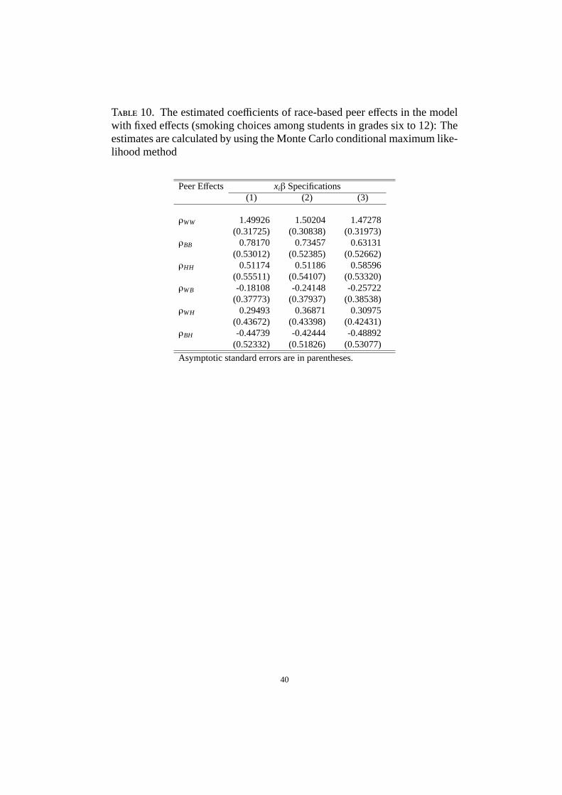
T 10. The estimated coefficients of race-based peer effects in the modelwith fixed effects (smoking choices among students in grades six to 12): Theestimates are calculated by using the Monte Carlo conditional maximum like-lihood method

Peer Effects xiβ Specifications(1) (2) (3)

ρWW 1.49926 1.50204 1.47278(0.31725) (0.30838) (0.31973)

ρBB 0.78170 0.73457 0.63131(0.53012) (0.52385) (0.52662)

ρHH 0.51174 0.51186 0.58596(0.55511) (0.54107) (0.53320)

ρWB -0.18108 -0.24148 -0.25722(0.37773) (0.37937) (0.38538)

ρWH 0.29493 0.36871 0.30975(0.43672) (0.43398) (0.42431)

ρBH -0.44739 -0.42444 -0.48892(0.52332) (0.51826) (0.53077)

Asymptotic standard errors are in parentheses.

40

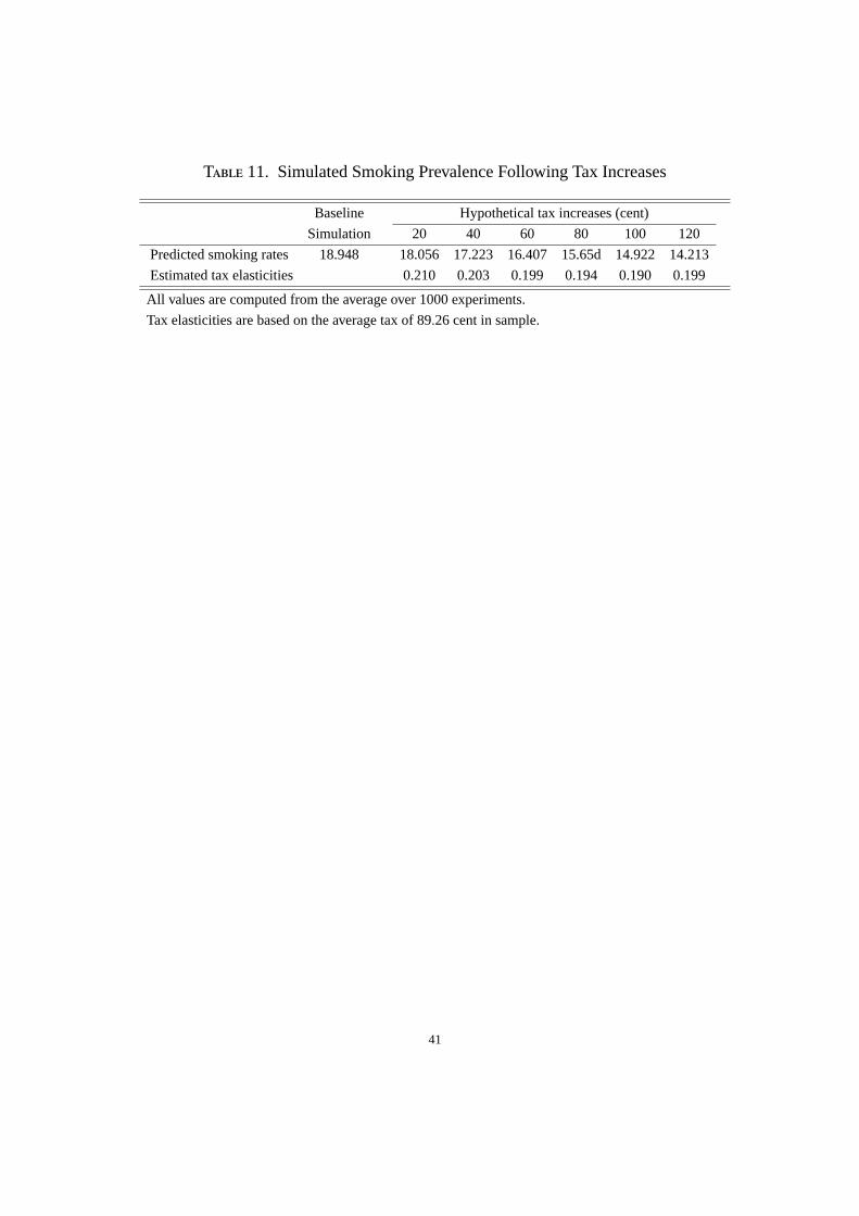
T 11. Simulated Smoking Prevalence Following Tax Increases

Baseline Hypothetical tax increases (cent)

Simulation 20 40 60 80 100 120

Predicted smoking rates 18.948 18.056 17.223 16.407 15.65d 14.922 14.213

Estimated tax elasticities 0.210 0.203 0.199 0.194 0.190 0.199

All values are computed from the average over 1000 experiments.

Tax elasticities are based on the average tax of 89.26 cent in sample.

41

T 12. Decomposition of Tax Effects on Smoking Prevalence

Hypothetical tax increases (cent)

Type of effects 20 40 60 80 100 120

Total effects -0.892 -1.725 -2.540 -3.294 -4.026 -4.735

Direct effects -0.541 -1.070 -1.600 -2.121 -2.614 -3.106

Social multipliers 1.649 1.612 1.588 1.553 1.540 1.525

All values are computed from the average over 1000 experiments.

Social multiplier is defined by the ratio of total effect to direct effect.

42

T 13. Simulated Smoking Prevalence Following Implementation ofSchool-based Smoking Program 1

Baseline Hypothetical School Program increases (percent)

Simulation 10 20 30 40 50

Predicted smoking rates 18.640 18.078 17.924 17.522 17.172 16.813

Estimated elasticities 0.082 0.052 0.054 0.053 0.053

All values are computed from the average over 1000 experiments.

Elasticities are based on the average school program of 27.04 percent in sample.

43

A D. A T

T 14. The estimated coefficients of county characteristics : The estimatesare calculated by the Monte Carlo maximum likelihood methods

Parameters xiβ Specifications(Coefficient on) (1) (2) (3)

Persons 0-18 -0.00531 -0.00856 -0.00226(0.02280) (0.02216) (0.02218)

Persons 65+ 0.00251 0.00311 0.00332(0.00790) (0.00768) (0.00787)

Asian persons 0.00627 0.00618 0.00655(0.00530) (0.00521) (0.00525)

Black persons 0.00327 0.00290 0.00356(0.00344) (0.00334) (0.00341)

Hispanic persons 0.00491 0.00575 0.00531(0.00223) (0.00221) (0.00222)

Single-mother families 0.00550 0.01185 0.00581(0.01550) (0.01373) (0.01518)

One-person families -0.02210 -0.02406 -0.02212(0.00882) (0.00860) (0.00873)

Persons with grandchildren -0.04468 -0.04420 -0.04561(0.02475) (0.02395) (0.02453)

Persons who divorced -0.01008 -0.01058 -0.00903(0.01431) (0.01412) (0.01425)

Unemployed workers 0.04817 0.04412 0.04669(0.01418) (0.01388) (0.01400)

Workers with management job -0.01377 -0.01315 -0.01367(0.01210) (0.01164) (0.01160)

Workers with professional job -0.01541 -0.01704 -0.01614(0.01209) (0.01188) (0.01180)

Workers with construction job 0.01764 0.01721 0.01608(0.01191) (0.01140) (0.01161)

Workers with farming job -0.01132 -0.01089 -0.01188(0.01191) (0.01141) (0.01178)

Workers with sales and office job 0.00966 0.00675 0.00829(0.00844) (0.00816) (0.00814)

Workers with service job 0.00188 0.00190 0.00129(0.00983) (0.00931) (0.00957)

Persons below poverty level -0.00474 -0.00575 -0.00318(0.01062) (0.01013) (0.01028)

Persons graduated high school -0.01024 -0.01058 -0.00911(0.00596) (0.00580) (0.00595)

Persons graduated college 0.01706 0.01802 0.01838(0.00769) (0.00743) (0.00746)

(continued on next page)

Asymptotic standard errors are in parentheses.

44

Parameters xiβ Specifications(Coefficient on) (1) (2) (3)

(continued from previous page)

Persons enrolled in public schools 0.00192 0.00112 0.00196(0.00391) (0.00376) (0.00391)

Persons enrolled in high schools -0.02973 -0.02786 -0.03177(0.03017) (0.02911) (0.02927)

Persons enrolled in colleges -0.00853 -0.00784 -0.00872(0.01254) (0.01204) (0.01206)

Persons enrolled in graduate schools 0.07041 0.06842 0.06650(0.05416) (0.05306) (0.05368)

Persons in armed forces 0.02012 0.01924 0.01878(0.01215) (0.01184) (0.01196)

Persons in veteran status 0.01126 0.01234 0.01312(0.01091) (0.01049) (0.01089)

Persons imigrated from foreign countries -0.03224 -0.03264 -0.03157(0.01757) (0.01680) (0.01691)

Persons moved in last 5 years -0.01254 -0.01212 -0.01241(0.00362) (0.00346) (0.00350)

Median household income 0.35930 0.31293 0.36120(0.38911) (0.37372) (0.37826)

Median housing value -0.31850 -0.30472 -0.31418(0.09055) (0.08617) (0.08860)

Vacant housing units -0.00103 -0.00402 -0.00249(0.00264) (0.00129) (0.00271)

Private vehicles occupacy -0.00305 -0.00181 -0.00102(0.00272) (0.00258) (0.00260)

Urban area rate -0.00385 -0.00315 -0.00384(0.00136) (0.00257) (0.00128)

Crime index -0.01649 -0.01675 -0.01898(0.01373) (0.01334) (0.01386)

Juvenile crime 0.00732 0.00668 0.00880(0.01442) (0.01397) (0.01427)

Juveniles crime (drug abuse) 0.18146 0.19590 0.18956(0.16581) (0.16016) (0.16496)

Asymptotic standard errors are in parentheses.

45