Water Air Soil PollutDOI 10.1007/s11270-009-0030-z

Measuring Fluorescent Dye in the Bubblyand Sediment-Laden Surfzone

David B. Clark · Falk Feddersen ·Melissa M. Omand · R. T. Guza

Received: 25 September 2008 / Accepted: 10 February 2009© The Author(s) 2009. This article is published with open access at Springerlink.com

Abstract Decisions about recreational beach clo-sures would be enhanced if better estimates ofsurfzone contaminant transport and dilution wereavailable. In situ methods for measuring fluo-rescent Rhodamine WT dye tracer in the surf-zone are presented, increasing the temporal andspatial resolution over previous surfzone tech-niques. Bubbles and sand suspended by breakingwaves in the surfzone interfere with in situ opti-cal fluorometer dye measurements, increasing thelower bound for dye detection (≈ 1 ppb) and re-ducing (quenching) measured dye concentrations.Simultaneous turbidity measurements are usedto estimate the level of bubble and sand inter-ference and correct dye estimates. After correc-tion, root-mean-square dye concentration errorsare estimated to be < 5% of dye concentrationmagnitude, thus demonstrating the viability of insitu surfzone fluorescent dye measurements. Thesurfzone techniques developed here may be ap-plicable to other environments with high bubbleand sand concentrations (e.g., cascading riversand streams).

D. B. Clark (B) · F. Feddersen ·M. M. Omand · R. T. GuzaScripps Institution of Oceanography, UCSD,9500 Gilman Dr., mail code 0209, La Jolla, CA92093-0209, USAe-mail: clark@coast.ucsd.edu

Keywords Surfzone · Mixing · Dispersion ·Fluorometer · Turbidity · Fluorescent dyemeasurement

1 Introduction

Surfzone dispersion is important to many biolog-ical and physical processes, including the dilu-tion of contaminated runoff (e.g., Boehm 2003;Grant et al. 2005), phytoplankton transport (e.g.,Campbell and Bate 1988), and larval recruit-ment (e.g., Denny and Shibata 1989). However,few surfzone tracer dispersion studies have beenconducted, and measurement techniques are lessadvanced than those used further offshore. As aresult, surfzone tracer dispersion is poorly under-stood. Increased knowledge of transport and dilu-tion in the surfzone would enable beach managersto better minimize public exposure to shorelinepollution.

Fluorescent dye (e.g., Rhodamine WT, or flu-orescein), optically measured with a fluorometer,is commonly used to study tracer (i.e., pollutant)dispersion in both marine (e.g., Okubo 1971) andfreshwater (e.g., Csanady 1963) environments.Dye measurements are used to estimate eddydiffusivities and scale dependence (e.g., Okubo1971; Murthy 1976; Fong and Stacey 2003), tracertransport (e.g., Houghton 1997; Tilburg et al.2007), and other quantities. The observations of

Water Air Soil Pollut

diffusion and mixing can be used to calibrate nu-merical models.

Ideally, accepted in situ techniques using flow-through (e.g., Pritchard and Carpenter 1960) oropen-face (e.g., Ledwell et al. 2004) fluorome-ters could be adapted for surfzone use. However,surfzone waves and strong currents can damageinstrumentation, hamper deployment, and rendermany oceanographic instruments and platforms(i.e., boats) unusable. Breaking waves intermit-tently suspend optically interfering bubbles (e.g.,Deane 1997) and sediment (e.g., Brenninkmeyer1976; Yu et al. 1993), creating highly variableturbidity.

Measured dye fluorescence is altered bymany factors, including background fluorescence(Pritchard 1979), temperature, and suspendedsediment (Smart and Laidlaw 1977). Suspendedsediment increases apparent background fluo-rescence without dye in the water and reduces(quenches) concentration estimates when dye ispresent. However, the effect of suspended sed-iment on dye estimates varies with sedimenttype, color, and concentration (Smart and Laidlaw1977), and the effect of suspended sand in thesurfzone is unknown. The effect of surfzone bub-bles on in situ dye measurements is also unknown.Dye mass can also be lost to photochemical decay(e.g., Suijlen and Buyse 1994), adsorption (e.g.,Talbot and Boon 1975), and other factors (e.g.,Smart and Laidlaw 1977), but these processes arenot expected to be significant over the few-hourduration of most surfzone dispersion studies.

Previous surfzone dye measurements havebeen limited to bottle samples taken either atthe shoreline or near the visually estimated cen-ter of a spreading dye patch (Harris et al. 1963;Inman et al. 1971; Clarke et al. 2007). While sim-ple and inexpensive, the number and distributionof samples has been severely limited, with maxi-mum rates up to two bottle samples per minute(Clarke et al. 2007), and a maximum of four si-multaneous locations over several hours (Harriset al. 1963). These studies provided importantinitial estimates of surfzone dispersion but couldnot resolve cross-shore dye structure and used few(or single) dye patch or plume realizations. Insitu fluorometers allow for higher-frequency dyemeasurements, but have not been implemented

in the surfzone, possibly because of concerns thatsuspended bubbles and sand would degrade in-strument performance.

Instruments suitable for in situ surfzone mea-surement of fluorescent Rhodamine WT dye arediscussed in Section 2, along with possible mech-anisms causing high errors in some instruments.The specific instrumentation used here (Section 3)and testing procedures (Section 4) are described.The effects of surfzone bubbles and sand on in situRhodamine WT measurements are characterized,and results are given in Section 5. Errors in insitu surfzone fluorescence are estimated, recom-mendations are made for error reduction, andexample field applications are given in Section 6.Details of mixing and delay time within the mobileflow-through fluorometer system and estimatesof effective spatial resolution are given in theAppendix.

2 Considerations for in situ Surfzone RhodamineWT Measurement

Many commercial fluorometers are available. Twowidely used, open-face-type fluorometers (WETLabs ECO Triplet and Turner SCUFA) that mea-sure Rhodamine WT dye fluorescence D andturbidity τ were tested side-by-side in a naturalsurfzone without dye in the water to determinethe instruments’ responses to suspended bub-bles and sand from breaking waves. Light emit-ted near the dye excitation peak is fluorescedat a slightly longer wavelength (e.g., Guibault1990). The intensity of the fluoresced light isdetected at an angle to the excitation beam (scat-tering angle) and used to determine dye con-centration (Fig. 1). The WET Labs ECO Tripletmeasures D (0.1–400 ppb range) with 530 nm[30 nm full width half max (FWHM)] wavelengthexcitation, and 570 nm fluorescence detection(35 nm FWHM), and measures τ (0.03–100 nturange) at 660 nm wavelength. ECO Triplet Dand τ both use 117◦ scattering angles. The TurnerSCUFA measures D (0.04–400 ppb range) with530 nm (40 nm FWHM) wavelength excitation,and 600 nm (40 nm FWHM) fluorescence de-tection, and measures τ (0.1–400 ntu∗ range) at530 nm. SCUFA D and τ both use 90◦ scattering

Water Air Soil Pollut

excitation light fluoresced andscattered light

dye, bubbles, and sand in thesample volume

instrument face

scattering angle

lightsource

fluorescence detector

filter

Fig. 1 Schematic of fluorometer optics (ECO Triplet ex-ample). Light emitted near the excitation peak of Rho-damine WT is fluoresced by the dye at a longer wavelengthand measured by the detector. When dye concentrationsare low, bubbles and sand in the sample volume (centershaded region) scatter excitation light from the instrumenttowards the dye fluorescence detector. Overlap betweenthe instrument excitation spectrum and the fluorescencedetection spectrum allows backscattered excitation light tobe falsely interpreted as an elevated dye concentration inthe sample volume. When dye concentrations are not low,bubbles and sand reduce the amount of fluoresced lightreaching the detector, and measured dye concentrationsare reduced. Bubbles and sand also backscatter light fromthe turbidity light source into the turbidity detector (notshown), increasing measured τ

angles. ECO Triplet and SCUFA τ , with units ntuand ntu∗, respectively, are similar but not equiva-lent due to instrumental differences (Section 3.2).

The instruments were mounted 1 m apart, sothey were close enough to measure similar tur-bidities but far enough apart to eliminate inter-ference. Both the ECO Triplet (Fig. 2a) and theSCUFA (Fig. 2b) recorded spurious dye mea-surements (nonzero dye measurements when nodye is present) in response to τ from surfzonebubbles and sand. The ECO Triplet recorded verylittle spurious dye (< 0.8 ppb), while the SCUFArecorded large spurious dye measurements (upto 17 ppb) that were highly correlated withturbidity τ .

The SCUFA and ECO Triplet measure Rho-damine WT fluorescence with different opti-cal elements and angles. Ideally, narrow-banded,

nonoverlapping optical filters on the source anddetection elements prevent excitation light frombeing detected as dye. However, nonideal opti-cal filters allow excitation light, backscattered offbubbles and sand (Fig. 1), to pass through thedetection filter and to be measured as elevateddye concentrations. The SCUFA optical filtershave a slightly wider pass-band than the ECOTriplet, possibly increasing SCUFA spurious dyemeasurements. However, the SCUFA filter cen-ters are also 10 nm further apart than the ECOTriplet, slightly reducing this effect. The intensityof light scattered by surfzone bubbles and sand in-creases with a reduction in scattering angle (Zegeet al. 2006). Therefore, the smaller SCUFA scat-tering angle increases the excitation light incidenton the detection filter, enhancing spurious dyemeasurements.

Although the SCUFA accurately measuresRhodamine WT in many environments, the com-bined effects of filters and scattering angle make

0

5

10

15 WET Labs ECO Tripleta

D (

ppb)

τ (

ntu)

0

10

20

30

0 100 200 300

0

5

10

15 Turner SCUFA

time (s)

b

D (

ppb)

τ (

ntu*

)

0

10

20

30

D (dye)

τ (turbidity)

Fig. 2 Field measurements of spurious D (black) and τ

(gray) vs time with no dye in the water for a WET LabsECO Triplet and b Turner SCUFA. The instruments weredeployed midsurfzone, 0.5 m above the seabed in 1 mdepth, and separated 1 m in the alongshore at ScrippsBeach, CA, with small spilling waves. Seaward of the sur-fzone, significant wave height was 0.5 m and peak periodwas 15 s. Note turbidity units (ntu, ntu∗) are similar but notequivalent due to instrumental differences (Section 3.2)

Water Air Soil Pollut

the SCUFA dye estimate more sensitive to sur-fzone bubbles and sand (spurious dye valuessometimes reached 80 ppb, not shown) than theECO Triplet. Further testing to determine the ef-fect of surfzone bubbles and sand on ECO Tripletdye measurements is described below (Section 5).

3 Surfzone Dye Fluorescence Instrumentation

In situ open-face-type (frame-mounted, fixed lo-cation) and flow-through-type (mobile, jet-ski-mounted, Fig. 3) fluorometer systems were usedto measure Rhodamine WT dye concentration(D) in the surfzone. Fixed-location fluorometersprovide much higher temporal resolution andlonger sampling periods than previous hand-filledbottle methods, but extensive spatial coverage isprecluded by cost and logistics. Increased spatialcoverage is provided by a jet-ski-mounted fluo-rometer system. The jet ski allows fast repeatedcross- and alongshore transects though the sur-fzone where traditional boats and submersiblescannot go. Simultaneous turbidity (τ ) measure-ments are used to estimate relative bubble andsand interference in the instrument sample vol-ume and to correct estimates of D. These in-struments can also be used to measure surfzonechlorophyll-a, but the methodology differs fromthat of dye (Omand et al. 2009).

electricpump

debubbler

bubbles, foam, air

SCU

FAtu

rbid

ity

Wetstarfluorometer

flow-through head

intake, 20 cm below the water surface

thermistor

Fig. 3 Schematic of jet ski mounted WS flow-throughsystem (not to scale)

WET Labs ECO Triplet open-face-type fluo-rometers (hereafter ET) were used to measuredye concentration D and backscatter turbidity τ

(see Section 2 for specifications), and were frame-mounted at fixed locations in the field. The ETsaveraged 8 Hz data to yield sampling rates of0.89 Hz in the laboratory and 0.23 Hz in the field.

The jet-ski-mounted, flow-through fluorome-ter/turbidity sensor system (hereafter WS) con-sisted of a WET Labs Wetstar fluorometer(470 nm excitation wavelength, 570 nm fluo-rescence detection, 0.11–400-ppb range) and aTurner SCUFA turbidity sensor (see Section 2 forspecifications) with flow-through cap. Althoughthe SCUFA is capable of measuring both flu-orescence and turbidity (Section 2), the surf-zone fluorescence signal was noisy (Fig. 2). Here,the SCUFA (robust enough for surfzone con-ditions) is used only for its flow-through tur-bidity measurement. Water, drawn through thejet-ski-mounted intake boom from 20 cm belowthe surface with an electric pump, passes througha debubbler, the SCUFA turbidity sensor, and,finally, the Wetstar fluorometer (Fig. 3). The de-bubbler (a small 200-ml chamber) allows air toescape from the top and water to flow out of thebottom, reducing the number of large bubbles en-tering the optical instruments. The flow-throughsystem hoses and debubbler (Fig. 3) smooth sharpgradients in dye occurring over times less than2.4 s, and delay dye measurements relative toGPS positions (Appendix). Dye fluorescence D,turbidity τ , water temperature (measured at theend of the intake boom), and GPS position aresampled at 5 Hz. Data are both logged onboardand transmitted to a shore station, allowing real-time analysis and adaptive sampling. A handlebar-mounted screen displays real-time data and a localmap of position, allowing repeated sampling ofpredetermined transects.

3.1 Fluorometer Calibrations

Fluorometers were calibrated at four tempera-tures (7–24 ◦C range) using nine known concen-trations of Rhodamine WT (0–400-ppb range) infiltered (to remove particles) seawater. Salinity,alkalinity, and pH all weakly affect dye fluores-cence (Feuerstein and Selleck 1963; Smart and

Water Air Soil Pollut

0 20 40 60 80 1000

20

40

60

80

sand concentration (g/L)

τ (

ntu,

ntu

*)

ET (ntu)WS (ntu*)

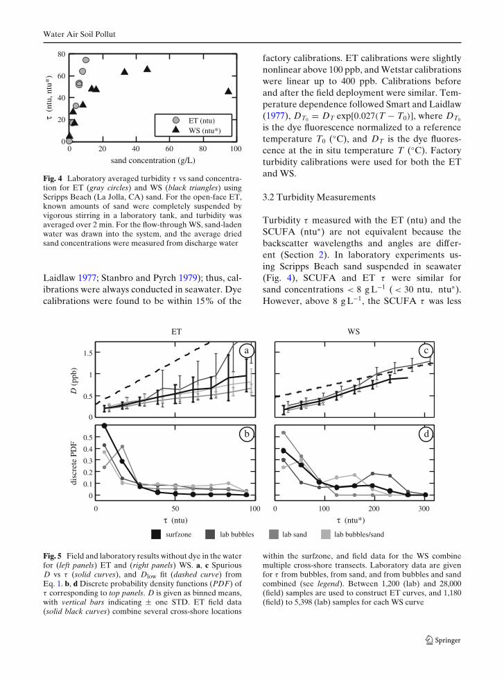
Fig. 4 Laboratory averaged turbidity τ vs sand concentra-tion for ET (gray circles) and WS (black triangles) usingScripps Beach (La Jolla, CA) sand. For the open-face ET,known amounts of sand were completely suspended byvigorous stirring in a laboratory tank, and turbidity wasaveraged over 2 min. For the flow-through WS, sand-ladenwater was drawn into the system, and the average driedsand concentrations were measured from discharge water

Laidlaw 1977; Stanbro and Pyrch 1979); thus, cal-ibrations were always conducted in seawater. Dyecalibrations were found to be within 15% of the

factory calibrations. ET calibrations were slightlynonlinear above 100 ppb, and Wetstar calibrationswere linear up to 400 ppb. Calibrations beforeand after the field deployment were similar. Tem-perature dependence followed Smart and Laidlaw(1977), DT0 = DT exp[0.027(T − T0)], where DT0

is the dye fluorescence normalized to a referencetemperature T0 (◦C), and DT is the dye fluores-cence at the in situ temperature T (◦C). Factoryturbidity calibrations were used for both the ETand WS.

3.2 Turbidity Measurements

Turbidity τ measured with the ET (ntu) and theSCUFA (ntu∗) are not equivalent because thebackscatter wavelengths and angles are differ-ent (Section 2). In laboratory experiments us-ing Scripps Beach sand suspended in seawater(Fig. 4), SCUFA and ET τ were similar forsand concentrations < 8 g L−1 ( < 30 ntu, ntu∗).However, above 8 g L−1, the SCUFA τ was less

0

0.5

1

1.5

ET

D (

ppb)

a

0 50 100

0

0.1

0.2

0.3

0.4

0.5

τ (ntu)

disc

rete

PD

F

b

WS

c

0 100 200 300

τ (ntu*)

d

surfzone lab bubbles lab sand lab bubbles/sand

Fig. 5 Field and laboratory results without dye in the waterfor (left panels) ET and (right panels) WS. a, c SpuriousD vs τ (solid curves), and Dlow fit (dashed curve) fromEq. 1. b, d Discrete probability density functions (PDF) ofτ corresponding to top panels. D is given as binned means,with vertical bars indicating ± one STD. ET field data(solid black curves) combine several cross-shore locations

within the surfzone, and field data for the WS combinemultiple cross-shore transects. Laboratory data are givenfor τ from bubbles, from sand, and from bubbles and sandcombined (see legend). Between 1,200 (lab) and 28,000(field) samples are used to construct ET curves, and 1,180(field) to 5,398 (lab) samples for each WS curve

Water Air Soil Pollut

responsive to sand than the ET. The SCUFA τ

sensor saturates near 75 ntu∗, at sand concen-trations > 20 g L−1 that are not expected abovethe bottom boundary layer in the surfzone. Addi-tional tests (Fig. 5) show that SCUFA τ > 75 ntu∗can be produced by bubbles or a combination ofbubbles and sand, but not by sand alone. SCUFAτ , well beyond the recommended 100 ntu∗ upperlimit (Turner Designs SCUFA manual, revision2.1), are used because they prove useful for errorestimation and dye correction in the WS instru-ment package (Section 6). The τ response to bub-ble void fraction was not measured.

4 Instrument Testing Methods

The effects of surfzone-bubble and sand-inducedturbidity τ on dye measurements D were ob-served both with and without dye in the water. Ex-periments without dye were conducted in both thefield (surfzone) and the laboratory. However, con-trolled dye concentrations could not be producedin the field, so tests with known (non-zero) dyeconcentrations were performed in the lab whereτ levels were varied by altering the amount ofsuspended bubbles and sand. To apply laboratory-based results to the field, it is assumed that naturalsurfzone τ over a sand bottom is primarily causedby bubbles and sand (i.e., not from mud, organicmatter, etc.).

4.1 Field Methods

ET and WS instruments were tested over sev-eral days in the surfzone at Huntington Beach,California, where significant wave height wasabout 1 m, peak periods ranged from 14 to 16 s,and hourly surfzone averaged alongshore currentsreached 0.5 m s−1. Huntington Beach sand is atan, medium-grained quartz typical of the South-ern California coast. Four ETs were deployed invarious cross-shore locations between the shore-line and 4 m mean water depth. The ETs weremounted nominally 0.5 m above the bed with thesensor facing downward at 30 degrees from verti-cal. Collocated temperature measurements wereused for ET dye calibration (Section 3.1). Thejet-ski-mounted WS was driven on ≈ 200-m-long

cross-shore transects from seaward of the surfzonetowards the shore (inbound transect) until the jetski turned around near the shoreline (≈ 0.5 mwater depth) and returned offshore (outboundtransect). WS field data were corrected for delaytime (relative to GPS positions) within the flow-through system (Appendix).

4.2 Laboratory Methods

Laboratory experiments with and without dye inthe water were conducted for both the open-faced ET and the flow-through WS system. Black(to reduce reflected light) containers were filledwith 15 l of filtered seawater and five dye con-centrations (0–238 ppb). The ET was held in thecontainer at midwater depth (≈ 15 cm), and forthe WS, the intake and discharge hoses weremounted near the bottom of the container. Bub-bles (≈ 0.1–5 mm diameter), roughly represen-tative of those injected into the surfzone bybreaking waves (Deane and Stokes 1999), wereadded using an aquarium aerator. Scripps Beachsand, a tan, medium-grained quartz, was addedby hand. Each system was perturbed with bub-bles; then with sand; and, finally, with bubblesand sand combined. Bubbles and sand were sus-pended by vigorous stirring, allowed to settle, andthen the process was repeated. It was unknownif the bubble and sediment size distribution of astirred laboratory container closely representedthat suspended in a natural surfzone. However,the amounts of bubbles and sand in the laboratorywere varied so the turbidity range spanned thatfound in the field.

5 Results

5.1 Field and Laboratory Without Dye

Field and laboratory data (D and τ ) without dyein the water were collected with the ET (Fig. 5a,b) and the WS (Fig. 5c, d) instruments. Spuriousdye concentrations D (when no dye is present)increase with turbidity τ in both field and labo-ratory measurements, consistent with Smart andLaidlaw (1977). High τ events are infrequent inthe surfzone for both instruments (Fig. 5b, d),

Water Air Soil Pollut

resulting in low mean spurious D (0.25 ppb forET, and 0.39 ppb for WS) in the surfzone.

The standard deviation (STD) of spurious dyemeasurements (indicated by vertical bars) in-creases with τ for the ET (Fig. 5a) but remainsnearly constant for the WS (Fig. 5c). ET labora-tory D results are similar to the surfzone, wherecombined bubble/sand results are the closest tothe field (Fig. 5a). WS lab results are also similarto the surfzone (Fig. 5c), but only the bubble-perturbed test produced the full range of observedsurfzone turbidity (because of the strongly nonlin-ear τ response to sand, Section 3.2).

Spurious dye measurements are small; how-ever, the integral over many spurious measure-ments in time (ET) or space (WS) can effect dyeconcentration statistics (e.g., total dye mass, dyepatch/plume width). For example, if the WS wasdriven on a cross-shore transect without dye inthe water, the inclusion of spurious dye measure-ments would suggest that dye, and the resulting

plume/patch width, spanned the entire transect.To remove spurious dye measurements for bothinstruments in the surfzone, a lower bound for dyedetection Dlow is estimated by a fit to D > 99%of the spurious surfzone D in each bin vs binnedτ . The disadvantage of this approach is that itsets a lower limit on measurable dye concentra-tion and the resultant size and duration that adye patch/plume can be observed. However, it issuggested that D below Dlow be set equal to zeroto avoid biasing dye statistics. The fit (Fig. 5a, c,dashed black line) to surfzone field data withoutdye for each instrument, respectively, is

Dlow = ατ + C , (1)

where α and C are fit constants and Dlow is inppb. For the ET, α = 0.02 ppb · ntu−1, and C =0.3 ppb, and for the WS, α = 0.01 ppb · ntu∗−1, andC = 0.46 ppb.

ET

bubbles

%ΔD

a

−20

−10

0

sand

%ΔD

b

−20

−10

0

bubbles/sand

τ (ntu)

%ΔD

c

0 25 50 75 100

−20

−10

0

WS

d

−40

−20

0

e

−40

−20

035 ppb70 ppb142 ppb238 ppb

τ (ntu*)

f

0 100 200 300 −40

−20

0

Fig. 6 Percent change in measured dye %�D(Eq. 2) vs τ from a, d bubbles; b, e sand; andc, f bubbles and sand combined, for (left panels) ET and(right panels) WS with four dye concentrations in the lab(see legend). %�D are given as binned means, with vertical

bars indicating ± one STD. Between 550 and 860 ET and3,600 and 5,400 WS samples are used to construct eachcurve. Dashed black lines in c and d show fits (Eq. 5)to binned mean data

Water Air Soil Pollut

5.2 Laboratory with Dye

Four known dye concentrations (D0) were per-turbed with bubbles (Fig. 6a, d), sand (Fig. 6b, e),and a combination of bubbles and sand (Fig. 6c,f) for ET (Fig. 6a–c) and WS (Fig. 6d–f), respec-tively. Changes in measured dye concentrationD are given as percent change %�D from theunperturbed known D0

%�D = 100 (D − D0)/D0 . (2)

The mean %�D is almost always negative (i.e.,quenching) and is similar for all dye concentra-tions (curves within each panel of Fig. 6 over-lay each other). This concentration-independent%�D is consistent with Smart and Laidlaw (1977)for τ -induced quenching of Rhodamine WT, butcontrasts with the concentration-dependent τ -induced quenching of chlorophyll-a (Omand et al.2009). The STD (vertical bars) about the mean%�D increases with τ for the ET, and to a lesserextent for the WS. The relationship between ET%�D and τ is similar for bubbles, sand, andbubbles and sand combined (i.e., curves in all leftpanels are similar), and the maximum decrease(%�D ≈ −20%, binned mean minus one STD)due to τ occurs at near full-scale turbidity val-ues. However, bubbles affect the WS differentlythan sand (Fig. 6d, e), with bubbles producing τ

up to 300 ntu∗ with moderate quenching effects(binned mean %�D minus one STD as largeas −25%), and sand producing τ up to 75 ntu∗with large quenching effects (binned mean %�Dminus one STD as large as −40%). The largeWS sand-quenching effect at moderate τ valuesis consistent with very high sand concentrations(that block fluoresced light) required to approachthe 75 ntu∗ saturation point for sand-induced τ

(Fig. 4).

6 Dye Measurement Corrections

Dye measurement errors are reduced by dis-carding dye data points with turbidity τ abovea threshold, and correcting the remaining dyefor τ -induced quenching. ET data were removedwhen τ > 90 ntu to exclude the increased scatter

in quenching (Fig. 6c) near and beyond the in-strument τ saturation point (100 ntu). WS datawere removed when τ > 300 ntu∗, the highest lab-observed τ (and, thus, the limit of lab-based τ

correction). The combination of discarding high τ

data and correcting the remaining D for τ -inducedquenching is hereafter called correction.

Surfzone fluorometers encounter bubbles andsand suspended by breaking waves and strongcurrents. The ET turbidity sensor cannot distin-guish between bubbles and sand. However, theeffects of bubble- and sand-induced τ on ET dyequenching are similar (Fig. 6a, b), and the curvederived from the combination of bubbles and sand(dashed line in Fig. 6c) is used for ET corrections.In contrast, bubbles- and sand-induced τ producevery different dye-quenching effects in the WS(Fig. 6d, e), but, as with the ET, the instrumentcannot distinguish between τ from bubbles andτ from sand. In the present application, the jet-ski-mounted WS system samples water 20 cmbelow the surface where average sand concentra-tions are expected to rarely exceed 1 g L−1 (e.g.,Beach and Sternberg 1992; Yu et al. 1993; Beachand Sternberg 1996; Ogston and Sternberg 2002).Even extreme sand concentrations (> 20 g L−1)only result in τ up to 75 ntu∗ (Fig. 4) with theWS τ sensor, leaving about one third of the fielddata with higher τ than sand alone can produce(Fig. 5d). Therefore, bubbles are assumed to bethe τ source, and WS dye measurement correc-tions are made using the bubble-quenching curve(Fig. 6d).

The relationship between binned mean %�D(Eq. 2) and τ are used to correct for τ -induceddye quenching. The fits to ET bubbles and sandcombined (Fig. 6c, dashed black line) and WSbubbles only (Fig. 6d, dashed black line) have theform

%�D = 100 βτ . (3)

Substituting Eq. 2 into Eq. 3 yields

D − D0

D0= βτ , (4)

where the fit constant is β = 1.2 × 10−3 ntu−1

(ET) and β = 0.91 × 10−3 ntu∗−1 (WS). EquatingD0 to corrected dye concentration Dc, and D to

Water Air Soil Pollut

%ΔD

ET

a

−30

−20

−10

0

10

unperturbedraw datacorrected

τ (

ntu)

time (s)

b

0 50 100 150 2000

50

100

c

WS

−30

−20

−10

0

10

time (s)

d

0 50 100 150 2000

100

200

300

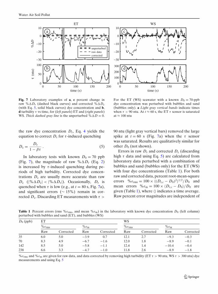
Fig. 7 Laboratory examples of a, c percent change inraw %�Dr (dashed black curves) and corrected %�Dc(with Eq. 5, solid black curves) dye concentration and b,d turbidity τ vs time, for (left panels) ET and (right panels)WS. Thick dashed gray line is the unperturbed %�D = 0.

For the ET (WS) seawater with a known D0 = 70-ppbdye concentration was perturbed with bubbles and sand(bubbles only). a Light gray vertical bands indicate timeswhen τ > 90 ntu. At t ≈ 60 s, the ET τ sensor is saturatedat ≈ 100 ntu

the raw dye concentration Dr, Eq. 4 yields theequation to correct Dr for τ -induced quenching

Dc = Dr

1 − βτ. (5)

In laboratory tests with known D0 = 70 ppb(Fig. 7), the magnitude of raw %�Dr (Eq. 2)is increased by τ -induced quenching during pe-riods of high turbidity. Corrected dye concen-trations Dc are usually more accurate than rawDc (|%�Dc| < |%�Dr|). Occasionally, Dr isquenched when τ is low (e.g., at t = 80 s, Fig. 7a),and significant errors (∼ 15%) remain in cor-rected Dc. Discarding ET measurements with τ >

90 ntu (light gray vertical bars) removed the largespike at t = 60 s (Fig. 7a) when the τ sensorwas saturated. Results are qualitatively similar forother D0 (not shown).

Errors in raw Dr and corrected Dc (discardinghigh τ data and using Eq. 5) are calculated fromlaboratory data perturbed with a combination ofbubbles and sand (bubbles only) for the ET (WS)with four dye concentrations (Table 1). For bothraw and corrected data, percent root-mean-squareerrors %εrms = 100 × 〈(Dr,c − D0)

2〉1/2/D0 andmean errors %εm = 100 × 〈Dr,c − D0〉/D0 aregiven (Table 1), where 〈〉 indicates a time average.Raw percent error magnitudes are independent of

Table 1 Percent errors (rms %εrms, and mean %εm) in the laboratory with known dye concentration D0 (left column)perturbed with bubbles and sand (ET), and bubbles (WS)

D0 (ppb) ET WS

%εrms %εm %εrms %εm

Raw Corrected Raw Corrected Raw Corrected Raw Corrected

35 6.0 5.0 −3.9 0.7 12.1 2.7 −9.3 −0.370 8.3 4.9 −6.7 −1.6 12.0 1.8 −8.9 −0.1142 8.5 5.0 −5.8 −1.1 12.4 1.4 −10.4 −0.4238 6.6 3.3 −4.7 −1.0 11.8 2.6 −8.9 −1.8

%εrms and %εm are given for raw data, and data corrected by removing high turbidity (ET τ > 90 ntu, WS τ > 300 ntu) dyemeasurements and using Eq. 5

Water Air Soil Pollut

D (

ppb)

a

0

20

40 D

r

Dc

b

Dc −

Dr (

ppb)

0

2

4

τ (

ntu)

time (s)

c

0 100 200 300 4000

50

100

Fig. 8 ET a raw and corrected dye concentration (Dr,Dc), b correction magnitude (Dc − Dr), and c τ vs timein the surfzone. The instrument was mounted 65 m fromthe shoreline, and 50 cm above the bottom. A dye patch(0.25 l of 21% by weight Rhodamine WT) was released10 m alongshore from the ET at t = 150 s. a Dc (gray curve)is estimated from Dr (black curve) and c corresponding τ

time series, using (Eq. 5). Light gray vertical bands indicatetimes when τ > 90 ntu (data are removed). Light grayhatching indicates times when Dr < Dlow (Eq. 1), and Dr,cshould be set to zero

concentration and are, generally, < 9% (< 13%)for ET (WS). For both ET and WS, correctionreduces rms (|%εrms| < 5%) and mean (|%εm| <

2%) errors. Error propagation into spatial dyemoments is nontrivial and depends on the shapeof the dye distribution, how realizations are aver-aged, and the assumed noise decorrelation scale.However, for a simple Gaussian example with 5%rms noise and a noise decorrelation scale equal toone STD of the Gaussian itself, the rms error inmeasured variance is 2%.

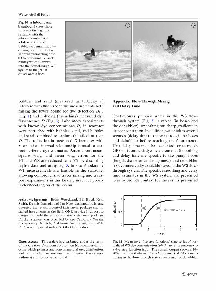
Examples of corrections to surfzone dye mea-surements are shown for ET (Fig. 8) and WS(Fig. 9). ET τ -induced quenching correctionsDc − Dr are small (< 4 ppb, Fig. 8b) comparedto dye variability (Fig. 8a). WS corrections aresimilarly small (< 1 ppb on the inbound transect),but they reach 9 ppb on the outbound transectwhen τ elevated by bubbly water is drawn into the

flow-through system when the jet ski drives overbubble-filled bores (Fig. 10b). On inbound tran-sects, bubbles are reduced by driving just in frontof the shoreward traveling bore (Fig. 10a). WS-corrected Dc on sequential inbound and outboundtransects have closer peak values than Dr.

High-turbidity events associated with increasederror are less frequent in the field than the lab(Fig. 5b); thus, ET dye measurement errors in thesurfzone are expected to be smaller than in thelaboratory (Table 1). In contrast, WS field errorsmay be increased relative to laboratory errorsby rare high-concentration sand events that areunaccounted for in lab estimates.

7 Summary

Open-face (ET) and flow-through (jet-ski-mounted WS) Rhodamine WT fluorometers forin situ surfzone sampling were tested. Surfzone

0

10

20

30

40

50

D (

ppb)

a

inbound, rawinbound, correctedoutbound, rawoutbound, corrected

−80 −60 −40 −20 00

100

200

cross−shore coordinate (m)

τ (

ntu*

) b

Fig. 9 WS a D and b τ vs cross-shore coordinate (pos-itive onshore, with shoreline at zero), for a single cross-shore transect pair, 575 m alongshore from the dye sourceduring a continuous release in the surfzone. Inbound andoutbound transect raw D and τ , and corrected D, areshown (see legend). Inbound corrected dye curve is ver-tically offset by +1 ppb for visibility. D > Dlow, and root-mean-square Dlow was 0.56 and 0.62 ppb for inbound andoutbound transects, respectively. About 1 min of data areshown

Water Air Soil Pollut

Fig. 10 a Inbound andb outbound cross-shoretransects through thesurfzone with thejet-ski-mounted WS.a Inbound transectbubbles are minimized bydriving just in front of ashoreward-traveling bore.b On outbound transects,bubbly water is drawninto the flow-through WSsystem as the jet skidrives over a bore

a b

bubbles and sand (measured as turbidity τ )interfere with fluorescent dye measurements bothraising the lower bound for dye detection Dlow

(Eq. 1) and reducing (quenching) measured dyefluorescence D (Fig. 6). Laboratory experimentswith known dye concentrations D0 in seawaterwere perturbed with bubbles, sand, and bubblesand sand combined to explore the effect of τ onD. The reduction in measured D increases withτ , and the observed relationship is used to cor-rect surfzone dye estimates. Percent root-mean-square %εrms and mean %εm errors for theET and WS are reduced to < 5% by discardinghigh-τ data and using Eq. 5. In situ RhodamineWT measurements are feasible in the surfzone,allowing comprehensive tracer mixing and trans-port experiments in this heavily used but poorlyunderstood region of the ocean.

Acknowledgements Brian Woodward, Bill Boyd, KentSmith, Dennis Darnell, and Ian Nagy designed, built, andoperated the jet-ski-mounted instrument package and in-stalled instruments in the field. ONR provided support todesign and build the jet-ski-mounted instrument package.Further support was provided by the California CoastalConservancy, NOAA, California Sea Grant, and NSF.DBC was supported with a NDSEG Fellowship.

Open Access This article is distributed under the termsof the Creative Commons Attribution Noncommercial Li-cense which permits any noncommercial use, distribution,and reproduction in any medium, provided the originalauthor(s) and source are credited.

Appendix: Flow-Through Mixingand Delay Time

Continuously pumped water in the WS flow-through system (Fig. 3) is mixed (in hoses andthe debubbler), smoothing out sharp gradients indye concentration. In addition, water takes severalseconds (delay time) to move through the hosesand debubbler before reaching the fluorometer.This delay time must be accounted for to matchGPS positions with dye measurements. Smoothingand delay time are specific to the pump, hoses(length, diameter, and roughness), and debubbler(not commercially available) used in the WS flow-through system. The specific smoothing and delaytime estimates in the WS system are presentedhere to provide context for the results presented

0 2 4 6 8

0

0.5

1

time (s)

norm

aliz

ed D

rise time = 2.4 s

Fig. 11 Mean (over five step functions) time series of nor-malized WS dye concentration (black curve) in response toa dye step function input. The system output shows a 10–90% rise time (between dashed gray lines) of 2.4 s, due tomixing in the flow-through system hoses and the debubbler

Water Air Soil Pollut

D (

ppb)

a

0

20

40

60

D (

ppb)

cross−shore coordinate (m)

b

−120 −100 −80 −60 −40 −20 00

20

40

inbound inbound, time corrected

outbound outbound, time corrected

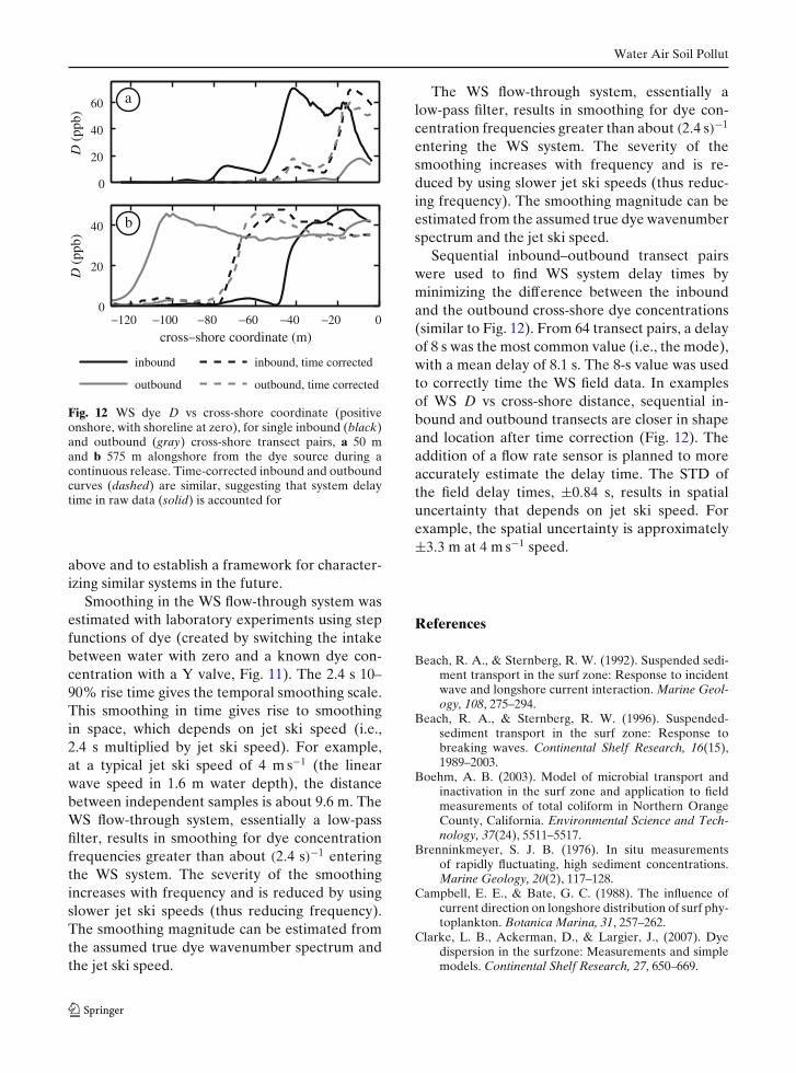
Fig. 12 WS dye D vs cross-shore coordinate (positiveonshore, with shoreline at zero), for single inbound (black)and outbound (gray) cross-shore transect pairs, a 50 mand b 575 m alongshore from the dye source during acontinuous release. Time-corrected inbound and outboundcurves (dashed) are similar, suggesting that system delaytime in raw data (solid) is accounted for

above and to establish a framework for character-izing similar systems in the future.

Smoothing in the WS flow-through system wasestimated with laboratory experiments using stepfunctions of dye (created by switching the intakebetween water with zero and a known dye con-centration with a Y valve, Fig. 11). The 2.4 s 10–90% rise time gives the temporal smoothing scale.This smoothing in time gives rise to smoothingin space, which depends on jet ski speed (i.e.,2.4 s multiplied by jet ski speed). For example,at a typical jet ski speed of 4 m s−1 (the linearwave speed in 1.6 m water depth), the distancebetween independent samples is about 9.6 m. TheWS flow-through system, essentially a low-passfilter, results in smoothing for dye concentrationfrequencies greater than about (2.4 s)−1 enteringthe WS system. The severity of the smoothingincreases with frequency and is reduced by usingslower jet ski speeds (thus reducing frequency).The smoothing magnitude can be estimated fromthe assumed true dye wavenumber spectrum andthe jet ski speed.

The WS flow-through system, essentially alow-pass filter, results in smoothing for dye con-centration frequencies greater than about (2.4 s)−1

entering the WS system. The severity of thesmoothing increases with frequency and is re-duced by using slower jet ski speeds (thus reduc-ing frequency). The smoothing magnitude can beestimated from the assumed true dye wavenumberspectrum and the jet ski speed.

Sequential inbound–outbound transect pairswere used to find WS system delay times byminimizing the difference between the inboundand the outbound cross-shore dye concentrations(similar to Fig. 12). From 64 transect pairs, a delayof 8 s was the most common value (i.e., the mode),with a mean delay of 8.1 s. The 8-s value was usedto correctly time the WS field data. In examplesof WS D vs cross-shore distance, sequential in-bound and outbound transects are closer in shapeand location after time correction (Fig. 12). Theaddition of a flow rate sensor is planned to moreaccurately estimate the delay time. The STD ofthe field delay times, ±0.84 s, results in spatialuncertainty that depends on jet ski speed. Forexample, the spatial uncertainty is approximately±3.3 m at 4 m s−1 speed.

References

Beach, R. A., & Sternberg, R. W. (1992). Suspended sedi-ment transport in the surf zone: Response to incidentwave and longshore current interaction. Marine Geol-ogy, 108, 275–294.

Beach, R. A., & Sternberg, R. W. (1996). Suspended-sediment transport in the surf zone: Response tobreaking waves. Continental Shelf Research, 16(15),1989–2003.

Boehm, A. B. (2003). Model of microbial transport andinactivation in the surf zone and application to fieldmeasurements of total coliform in Northern OrangeCounty, California. Environmental Science and Tech-nology, 37(24), 5511–5517.

Brenninkmeyer, S. J. B. (1976). In situ measurementsof rapidly fluctuating, high sediment concentrations.Marine Geology, 20(2), 117–128.

Campbell, E. E., & Bate, G. C. (1988). The influence ofcurrent direction on longshore distribution of surf phy-toplankton. Botanica Marina, 31, 257–262.

Clarke, L. B., Ackerman, D., & Largier, J., (2007). Dyedispersion in the surfzone: Measurements and simplemodels. Continental Shelf Research, 27, 650–669.

Water Air Soil Pollut

Csanady, G. T. (1963). Turbulent diffusion in Lake Huron.Journal of Fluid Mechanics, 17(3), 360–384.

Deane, G. B. (1997). Sound generation and air entrainmentby breaking waves in the surf zone. Journal of theAcoustical Society of America, 102(5), 2671–2689.

Deane, G. B., & Stokes, M. D. (1999). Air entrainmentprocesses and bubble size distributions in the surfzone. Journal of Physical Oceanography, 29, 1393–1403.

Denny, M. W., & Shibata, M. F. (1989). Consequences ofsurf-zone turbulence for settlement and external fer-tilization. American Naturalist, 134, 859–889.

Feuerstein, D. W., & Selleck, R. (1963). Fluorescent tracersfor dispersion measurements. Journal of the SanitaryEngineering Division, American Society of Civil Engi-neers, 89(SA4), 1–21.

Fong, D. A., & Stacey, M. T. (2003). Horizontal dispersionof a near-bed coastal plume. Journal of Fluid Mechan-ics, 489, 239–267.

Grant, S. B., Kim, J. H., Jones, B. H., Jenkins, S. A., Wasyl,J., & Cudaback, C. (2005). Surf zone entrainment,along-shore transport, and human health implicationsof pollution from tidal outlets. Journal of GeophysicalResearch, 110(C10025). doi:10.1029/2004JC002401.

Guibault, G. (Ed.) (1990). Practical Fluorescence, 2nd edn.Marcel Dekker, New York.

Harris, T. F. W., Jordaan, J. M., McMurray, W. R., Verwey,C. J., & Anderson, F. P. (1963). Mixing in the surfzone. International Journal of Air and Water Pollution,7, 649–667.

Houghton, R. W. (1997). Lagrangian flow at the foot of ashelfbreak front using a dye tracer injected into thebottom boundary layer. Geophysical Reasearch Let-ters, 24(16), 2035–2038.

Inman, D. L., Tait, R. J., & Nordstrom, C. E., (1971). Mix-ing in the surfzone. Journal of Geophysical Research,26, 3493–3514.

Ledwell, J. R., Duda, T. F., Sundermeyer, M. A., & Seim,H. E. (2004). Mixing in a coastal environment: 1. Aview from dye dispersion. Journal of Geophysical Re-search, 109(C10013). doi:10.1029/2003JC002194.

Murthy, C. R. (1976). Horizontal diffusion charateristics inLake Ontario. Journal of Physical Oceanography, 6,76–84.

Ogston, A. S., & Sternberg, R. W. (2002). Effect of wavebreaking on sediment eddy diffusivity, suspended-sediment and longshore sediment flux profiles in thesurf zone. Continental Shelf Research, 22, 633–655.

Okubo, A. (1971). Oceanic diffusion diagrams. Deep SeaResearch, 18, 789–802.

Omand, M. M., Feddersen, F., Clark, D. B., Franks, P. J. S.,Leichter, J. J., & Guza, R. T. (2009). The influenceof bubbles and sand on chlorophyll fluorescence mea-surements in the surfzone. Limnology and Oceanogra-phy: Methods (2009, in press).

Pritchard, D. W. (1979). Background problems in fluoro-metric dye measurement in natural water. Oceans, 11,572–582.

Pritchard, D. W., & Carpenter, J. H. (1960). Measurementsof turbulent diffusion in estuarine and inshore waters.Bulletin of the International Association of ScientificHydrology, 20, 37–50.

Smart, P. L., & Laidlaw, I. M. S. (1977). An evaluationof some fluorescent dyes for water tracing. Water Re-sources Research, 13(1), 15–33.

Stanbro, W. D., & Pyrch, D. A. (1979). Stability of Rho-damine WT in saline waters. Water Resources Re-search, 15(6), 1631–1632.

Suijlen, J. M., & Buyse, J. J. (1994). Potentials of photolyticRhodamine WT as a large-scale water tracer assessedin a long-term experiment in the Loosdrecht Lakes.Limnology and Oceanography, 36(6), 1411–1423.

Talbot, J. W., & Boon, M. J. (1975). The adsorption ofrhodamine on to suspended sediments. ICES Journalof Marine Science, 32(2), 128–132.

Tilburg, C. E., Houghton, R. W., & Garvine, R. W.(2007). Mixing of a dye tracer in the Delawareplume: Comparison of observations and simula-tions. Journal of Geophysical Research, 112(C12004).doi:10.1029/2006JC003928.

Yu, Y., Sternberg, R. W., & Beach, R. A. (1993). Kine-matics of breaking waves and associated suspendedsediment in the nearshore zone. Continental Shelf Re-search, 13(11), 1219–1242.

Zege, E. P., Katsev, I. L., Prikhach, A. S., Gilbert, G., &Witherspoon, N. (2006). Simple model of the opticalcharacteristics of bubbles and sediments in seawaterof the surf zone. Applied Optics, 45(25), 6577–6585.