Universität Leipzig Alfred-Wegener-InstitutFakultät für Physik- und für Polar- und Meeresforschung Geowissenschaften PotsdamInstitut für Geographie

Measuring and modeling of soil thermal

properties and ground heat flux

at two different sites at

Lena Delta, Siberia

Diploma thesis

submitted by

Katrin Fröb

matriculation number: 9762674

June 2011

Supervised by: Prof. Dr. Werner Kirstein

Universität Leipzig, Institut für Geographie

Dr. Julia Boike

Alfred-Wegener-Institut für Polar- und Meeresforschung

Forschungsstelle Potsdam

“Doubt is the beginning of wisdom.”

Aristotle

Table of contents

I List of abbreviations, symbols, constants...................................................................iv

II List of figures.............................................................................................................vii

III List of tables.............................................................................................................. ix

1 Introduction – state of the art.......................................................................................1

2 Fundamentals.............................................................................................................4

2.1 Permafrost...........................................................................................................4

2.2 Distribution of permafrost.....................................................................................5

2.3 Cryogenic processes...........................................................................................8

2.3.1 Segregation ice............................................................................................8

2.3.2 Frost heave..................................................................................................9

3 Study site description................................................................................................11

3.1 The Lena Delta..................................................................................................11

3.2 Samoylov...........................................................................................................15

3.3 Kurungnakh.......................................................................................................17

4 Methods....................................................................................................................20

4.1 Field work..........................................................................................................20

4.1.1 Soil sampling..............................................................................................20

4.1.2 Borehole instrumentation...........................................................................22

4.2 Lab measurements............................................................................................25

4.2.1 Importance of measuring the physical properties of the soil......................25

4.2.2 The particle size distribution.......................................................................25

4.2.3 The soil ice content and porosity................................................................25

i

ii Table of contents

4.2.4 The soil organic content.............................................................................26

4.2.5 The soil carbon content..............................................................................27

4.2.6 The soil density..........................................................................................27

4.3 Determination of soil thermal properties............................................................30

4.3.1 The volumetric and specific heat capacity..................................................30

4.3.2 The thermal conductivity from soil temperature data

(Conduction method)...................................................................................30

4.4 Modeling of thermal conductivity........................................................................32

4.4.1 Calculating the soil thermal conductivity using the

de Vries method (1952)..............................................................................32

4.3.2 The Johansen model (1975)......................................................................34

4.3.3 Conductivity after Endrizzi et al. (2011)......................................................35

5 Results......................................................................................................................37

5.1 Samoylov...........................................................................................................37

5.1.1 Soil temperature profile..............................................................................37

5.1.2 Soil physical properties..............................................................................38

5.1.3 Calculation of conductivity .........................................................................40

5.2 Kurungnakh.......................................................................................................43

5.2.1 Soil temperature profile..............................................................................43

5.2.2 Soil physical properties..............................................................................44

5.2.3 Calculation of conductivity..........................................................................46

5.3 Comparison.......................................................................................................48

5.3.1 Soil temperature profiles............................................................................48

5.3.2 Soil physical properties..............................................................................48

5.3.3 Calculation of conductivity..........................................................................49

6 Interpretation and discussion....................................................................................51

6.1 Error discussion for soil properties.....................................................................51

6.2 Measurement analysis.......................................................................................52

6.3 Modeling analysis..............................................................................................53

6.3.1 The de Vries (1952) method.......................................................................53

6.3.2 The Johansen (1975) method....................................................................54

6.3.3 The method by Endrizzi et al. (2011)..........................................................56

6.4 Soil carbon content............................................................................................56

Table of contents iii

7 Conclusion................................................................................................................58

Acknowledgements......................................................................................................61

IV Glossary.....................................................................................................................x

V Bibliography..............................................................................................................xii

Appendix

Appendix A...................................................................................................................xx

Appendix B..................................................................................................................xiii

I List of abbreviations, symbols, constants

a.r.l. above river level

a.s.l. above sea level

CCSM Community Climate System Model

CLM Community Land Model

e.g. for example

et al. and others

f. following page

ff. following pages

GCM General Circulation Model

GST ground surface temperature

HadCM3 Hadley Centre Coupled Model version 3

i.e. this means

MAAT mean annual air temperature

MAGT mean annual ground temperature

MATLAB Matrix Laboratory

MOSES Met Office Surface Exchange Scheme

SOCC soil organic carbon content

TOC total organic carbon

vol.% volumetric percent

WRB World Reference Base for Soil Resources

βai fraction parameter [-]

cv volumetric heat capacity [MJ m-³ K-1]

ch specific heat capacity [MJ kg-1 K-1]

dh thermal diffusivity [m² s-1]

fn weighting factor [-]

fsc soil organic fraction [-]

iv

I List of abbreviations, symbols, constants v

φ porosity of sample [vol.%]

Kc thermal conductivity of the continuous phase [W m-1 K-1]

Kdry soil dry thermal conductivity [W m-1 K-1]

Kdry, min soil mineral dry thermal conductivity [W m-1 K-1]

Ke Kersten number [-]

Kh soil thermal conductivity [W m-1 K-1]

Ks solid soil thermal conductivity [W m-1 K-1]

Ks,min mineral soil solid conductivity [W m-1 K-1]

Ksat soil saturated thermal conductivity [W m-1 K-1]

mds mass of dried sample [g]

mf mass of foil [g]

mI mass of ice content [g]

mt total mass of sample [g]

mw mass of wet sample [g]

mwf mass of wet sample + foil [g]

ρb bulk density [kg m-³]

ρsc soil carbon density [g cm-³]

ρt total density of sample [g cm-³]

SOCC soil organic carbon content [kg m-²]

T temperature [°C, K]

Tmeas (z, t) measured temperature in a certain depth over time [°C]

Tmod (z, t) modeled temperature in a certain depth over time [°C]

θA volumetric air content [-]

θI volumetric ice content [-]

θO volumetric organic content [-]

θS volumetric solid content [-]

θsat, volumetric water content for saturated soil [-]

θsat, min volumetric water content for mineral soil [-]

VA volume of air content [cm³]

VI volume of ice content [cm³]

VO volume of organic content [cm³]

VS volume of solid soil content [cm³]

Vt total sample volume [cm³]

wi mass fraction ice [-]

wO mass fraction organic [-]

z vertical coordinate [m]

vi I List of abbreviations, symbols, constants

ch,a specific heat capacity air = 0.00072 MJ kg-1 K-1

ch,i specific heat capacity ice = 2.0 MJ kg-1 K-1

ch,o specific heat capacity organic = 2.5 MJ kg-1 K-1

ch,s specific heat capacity solid material = 2.4 MJ kg-1 K-1

εs smoothing parameter = 4

Kdry,sc thermal conductivity dry organic soil = 0.1 W m-1 K-1

Kh,a thermal conductivity air = 0.025 W m-1 K-1

Kh,i thermal conductivity ice = 2.2 W m-1 K-1

Kh,o thermal conductivity organic = 0.25 W m-1 K-1

Kh,s thermal conductivity solid = 2.92 W m-1 K-1

Kliq thermal conductivity liquid water = 0.6 W m-1 K-1

ρA density of air = 1.29 kg m-³

ρI density of ice = 917 kg m-³

ρO density of organic = 1300 kg m-³

ρS density of solid content = 2650 kg m-³

ρsc, max maximum soil carbon density = 1.3 g cm-³

θsat,sc volumetric water content for saturated organic soil = 0.9

θi0 volumetric ice content, where water starts to affect soil thermal

conductivity = 0.15

θliq volumetric liquid water content, assumed 0 for analysed soils

II List of figures

Fig. 1: Illustration of permafrost components (modified after: FRENCH 2007: 84). ...........5

Fig. 2: Distribution of permafrost on the northern hemisphere

(source: BROWN ET AL. 1998). .............................................................................6

Fig. 3: Simplified permafrost development from north to south

(modified after: FRENCH 2007: 71). ....................................................................7

Fig. 4: Location of the Lena Delta within the Russian Federation and location of the

two study sites (source: ESA, RUSSIA MAP). .....................................................12

Fig. 5: Mean annual discharge of the Lena near the island of Stolb in the Lena

Delta (source: ARCTICNET 2011). ....................................................................13

Fig. 6: Aerial picture of Samoylov Island (source: BOIKE ET AL. 2007). ...........................15

Fig. 7: Thermokarst development in Yedoma landscapes, using the example of

Kurungnakh (source: MORGENSTERN ET AL. 2011: 1545). ....................................18

Fig. 8: Pürckhauer drill (A); sledge (B) and lever (C) (source: ECOTECH). ......................20

Fig. 9: Drilling equipment: (A) engine for penetrating the ground, (B) drilling head

with sample (Photo: J. Boike 2009). ...............................................................21

Fig. 10: Sample bag with sample and note of depth and direction of core

(Photo: J. Boike 2009). ..................................................................................22

Fig. 11: Installing of temeprature chain with (A) plastic tubes, (B) temperature

sensor, (C) temperature chain and (D) the data logger; the red line marks

the ground surface (Photo: J. Boike 2009). ....................................................23

Fig. 12: Surrounding of the bore hole on Kurungnakh one year after installing the

vii

viii II List of figures

temperature chain; the red line marks the former grounds surface

(Photo: M. Langer 2010). ...............................................................................24

Fig. 13: Overflow-cylinder as equipment for density measurement

(Photo: K. Fröb 2011). ...................................................................................28

Fig. 14: Temperature profiles from July 2009 to August 2010 of the different meas-

uring depths of the Samoylov core including the surface temperature;

depths are distances from 0 m downwards. GST is to be considered as

ground surface temperature. ..........................................................................37

Fig. 15: Physical properties of the Samoylov core. ......................................................39

Fig. 16: Thermal properties for the Samoylov core calculated by using different

models. ..........................................................................................................40

Fig. 17: Interpolated temperatures of the Samoylov core by using the conduction

method. ..........................................................................................................41

Fig. 18: Temperature profiles from July 2009 to August 2010 of the different meas-

uring depths of the Kurungnakh core including the surface temperature;

depths are distances from 0 m downwards. ..................................................43

Fig. 19: Physical properties of the Kurungnakh core. ..................................................44

Fig. 20: Thermal properties for the Kurungnakh core calculated by using different

models. ..........................................................................................................46

Fig. 21: Interpolated temperatures of the Kurungnakh core by using the conduction

method. ..........................................................................................................47

III List of tables

Table 1: Thermal properties of soil components (taken from: Farouki 1981b: 12).......33

ix

1 Introduction – state of the art

Permafrost areas have been under observation for a long time. Due to their special ap-

pearance in terms of landscape elements such as pingos or polygonal tundra they are

of interest for geomorphologists. For the construction of buildings and roads or

pipelines a detailed knowledge about the ground is necessary. A very specialised ve-

getation and an even more adapted fauna with many interesting microbiological pro-

cesses are of great interest for biologists. If nothing else, permafrost areas are fascinat-

ing because of their treeless vastness – in the very north – and their hostile environ-

ment.

Arctic and high-Arctic regions are complex ecosystems that respond quickly to chan-

ging ambient conditions. During these days permafrost regions are spotlighted mainly

in terms of global climate change. That is because climate change would affect those

extreme areas in a much more intense way than other regions (ROMANOVSKY ET AL. 2007).

Especially the topic of a release of stored carbon in the frozen soils is discussed by

many authors. According to POST ET AL. (1982) the upper 100 cm of tundra soils contain

about 14% of the worlds total soil carbon content. More recent studies were performed

by TARNOCAI ET AL. (2009) who estimates that approximately 33% of the global organic

carbon is stored between 0 and 100 cm depth in tundra soils. Added to this organic

content there is a currently frozen, thus immobile fraction of organic material stored in

the deeper soil layers. If permafrost thaws, this large carbon storage becomes poten-

tially accessible to increased microbial decomposition which presumably leads to in-

creased production of green house gases. Hence, it is conceivable that large perma-

frost areas convert into considerable atmospheric carbon sources under a warming cli-

mate. Due to this potential feedback mechanisms it seems to be crucial to include per-

mafrost in all projections of future climate.

During the last decades there has been great effort to develop general circulation mod-

els (GCM) which are able to predict future scenarios of the atmosphere under changing

climate conditions. Despite its potential importance in the global carbon cycle, perma-

frost is yet not included in the land atmosphere schemes of recent GCMs. According to

1

2 1 Introduction – state of the art

the third report of the Intergovernmental Panel on Climate Change (IPCC 2001: 491)

“there has been limited progress towards developing a permafrost model for use in cli-

mate models”. One of the major challenges is to close the gap between the GCMs and

the existing regional permafrost models. Efforts in this direction had been made,

among others, by STENDEL ET AL. (2007). The following fourth IPCC report (2007) con-

tains a whole section discussing Arctic and Antarctic processes related to global cli-

mate. KITABATA ET AL. (2006) predict in this report a poleward moving permafrost line with

a 50% reduction of the recent ground ice volume by 2030. Furthermore ANISIMOV &

RENEVA (2006) used the output of five different GCMs to predict the future permafrost

distribution in Russia. All models showed different results which was mainly caused by

uncertainties in the input parameters (ANISIMOV & RENEVA 2006).

For modelling permafrost and its response to a changing climate the soil thermal prop-

erties are crucial parameters. Those properties include the thermal conductivity, the

thermal diffusivity and the heat capacity of the ground. The thermal conductivity is the

ability of the soil to conduct heat, the heat capacity of a soil describes its ability to store

heat and the thermal diffusivity is the quotient of those two parameter. However, in the

vast Arctic region data on thermal soil properties are only sparsely available.

The soil heat capacity can be directly inferred if the soil composition is known. How-

ever, the determination of the thermal conductivity is very difficult, as it not only de-

pends on the soil. Other parameter are for example the vegetation cover of the soil,

water movement within the soil or the sun radiation. Especially lateral water movement

processes are hard to quantify. Therefore, the soil thermal conductivity is often para-

metrized according to accessible information on the soil. Many authors have developed

model approaches and calculations (e.g. GOODRICH 1980, LUNARDINI 1998, ZHANG &

KUSHWAHA 1998). For example HINZMANN ET AL. (1998) developed a model simulating

thermal processes in both the active layer and the underlying permafrost. GUYMAN ET AL.

(1980) developed a model for calculating freezing processes and GORI (1983) designed

a model to predict the thermal conductivity of unsaturated frozen soils. A good overview

about different models currently in use is given by RISEBOROUGH ET AL. (2008).

It is the objective of this work to show the differences of various models for simulating

the thermal properties of frozen ground. The focus rests on determining the thermal

conductivity, which is essential for the heat transport. The model results are compared

to each other and to measured data of heat diffusivity and by that the heat conductivity.

The models try to simulate the grounds thermal conductivity in two different soil cores.

Those cores are taken from two islands in the Lena Delta in Siberia by scientists of the

Alfred-Wegener-Institute in Potsdam.

1 Introduction – state of the art 3

The thesis is subdivided as followed: The second chapter includes a definition of per-

mafrost and processes that are related, followed by a description of the two dealt with

study sites in the Lena Delta in chapter 3. The used methods in this work are explained

in chapter 4, while the results of the measurements are given in the next chapter 5. Fi-

nally section 6 deals with the discussion of the results and in the end part 7 gives a

conclusion.

2 Fundamentals

2.1 Permafrost

According to DAVIS (2001: 2), permafrost is ground which has a “temperature lower than

0 °C” for “at least two consecutive years”, even over summer. This shall be understood

without “glaciers and ice caps” (HARRIS 1986: 1). FRENCH (2007: 83) widens the temper-

ature range to: “at or below 0 °C”. This doesn't necessarily mean that the water in per-

mafrost is already frozen at 0 °C. Because of higher pressures or salinity rates water

may stay unfrozen even with lower ambient temperatures. At the same time the pres-

ence of water – or ice – is not necessary to define permafrost. The Antarctic permafrost

for example contains “little or no ice” (FRENCH 2007: 83).

The upper part of the permafrost is called the active layer because it thaws in summer

and refreezes in autumn. It contains the roots of the vegetation and water movement

can take place. The lower part is the permafrost which stays frozen over the whole

year. Its depth varies due to different variables that will be described in the following

sub chapter. Within permafrost, patches of unfrozen soil may exist, the so called talik,

which is depicted in fig. 1. Taliks can be found in different sizes and locations, espe-

cially beneath rivers and lakes in permafrost areas because of warming effects due to

the superimposed water masses. Changing ambient conditions such as water content,

salinity, pressure or temperature are further reasons for taliks to form. These factors

are influenced by properties of the soil and the overall environmental conditions.

4

2.1 Permafrost 5

2.2 Distribution of permafrost

Most of the recent global permafrost can be found in the northern hemisphere; approx-

imately 22% of the land surface are underlain by frozen soil (BROWN ET AL. 1998). The

circumpolar countries, such as Russia, Canada, the U.S. or Norway, have different per-

centages of their area being underlain by permafrost. Those are, according to the

CANADIAN ENCYCLOPEDIA: Russia with 50% of its area underlain by permafrost, Alaska with

80% and Canada with 40 to 50%. Fig. 2 shows the current permafrost distribution on

the northern hemisphere and the projected permafrost boundary by the year 2100. This

boundary was simulated by using the five models of the ACIA report (2005).

Several factors limit the formation of permafrost, which can roughly be classified in “cli-

matic and terrain factors” (HARRIS 1986: 60).

Latitude and by that the angle of the sun radiation affect temperature and precipitation

– the main climatic factors. Snow for example plays a major role in insulating the

Fig. 1: Illustration of permafrost components (modified after: FRENCH 2007: 84).

6 2 Fundamentals

ground from the cold winter temperatures, so both the amount and duration of snow

cover affect the formation of permafrost. Of importance for the development of perma-

frost is also the mean annual air temperature (MAAT), although some authors, such as

HARRIS (1986: 60), state that the distribution of permafrost “does not correlate too well”

with the MAAT. This demonstrates the influence of factors other than the local temper-

ature conditions.

As terrain factors count the “local relief, vegetation, hydrology [and] nature of the soil or

rock” (HARRIS 1986: 60). Topography is important, especially in the mountains where

Fig. 2: Distribution of permafrost on the northern hemisphere (source: BROWN ET AL. 1998). The dotted line marks the predicted permafrost distribution in 2100 (source: ACIA 2005).

2.2 Distribution of permafrost 7

permafrost is usually thicker on the north facing hill due to lower insulation. Mountains

also have an effect on the local climate, such as building cold traps and sun exposed

spots, which again influences local vegetation. Vegetation on the other hand insulates

the ground from hot summer temperatures. It therefore plays a major role in the non

Arctic desert zones (HARRIS 1986). The interaction of all limiting factors defines the

spreading of permafrost on the land surface.

There is also a limitation of the depth of permafrost. Due to the geothermal gradient

permafrost can only be built up to a certain depth. This gradient varies in space, de-

pending on the heat conductivity of the underlain material (WILLIAMS & SMITH 1989). It is

therefore difficult to estimate the depth of permafrost only by surface temperatures

without considering the geothermal gradient (LACHENBRUCH & MARSHALL 1969).

Additionally there is some sub-sea permafrost on the continental shelves in the Arctic

Ocean which developed during the last glaciation when the water level was much

lower. Later, with rising water level, the shelves were flooded and the permafrost was

conserved under water (HARRIS 1986). Although the temperatures are below 0 °C this

type of permafrost contains a lot of fluid water instead of ice, due to the salinity of the

ocean water (DAVIS 2001). This soil is called permafrost because of the defining condi-

tion of year-round temperatures below 0 °C, even though the water in this soil is not

frozen at this temperature (WILLIAMS & SMITH 1989).

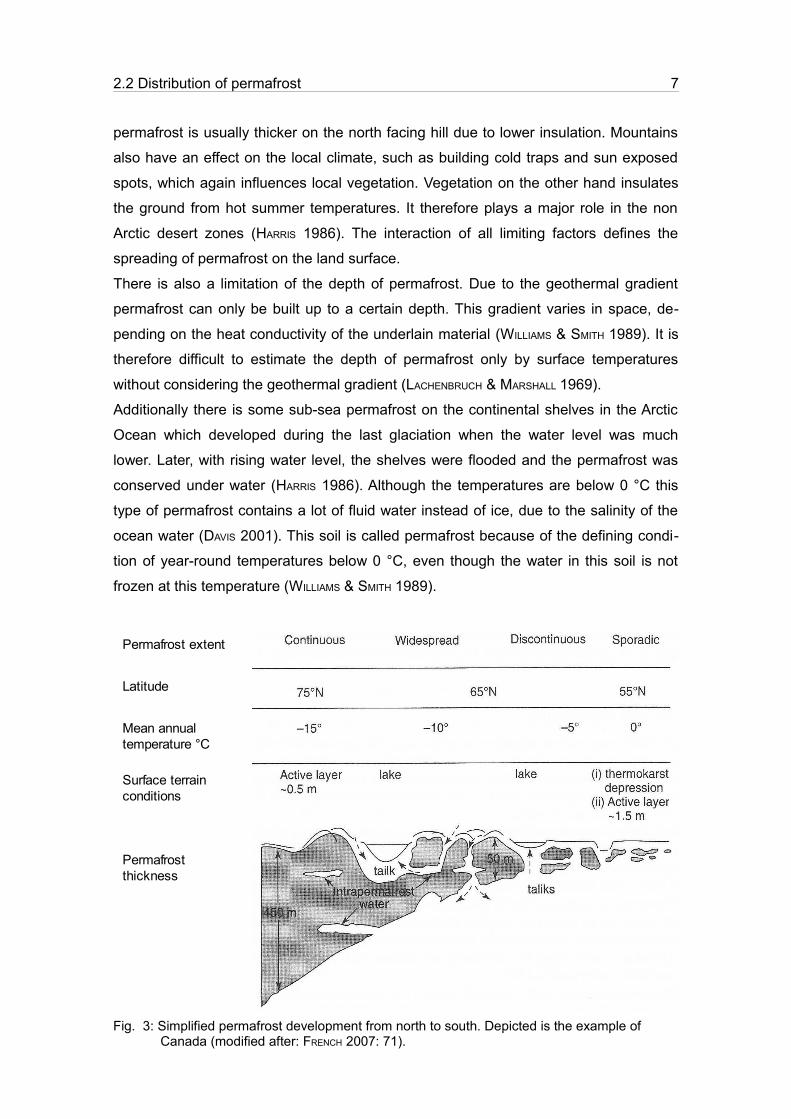
Fig. 3: Simplified permafrost development from north to south. Depicted is the example of Canada (modified after: FRENCH 2007: 71).

Permafrost extent

Latitude

Mean annualtemperature °C

Surface terrainconditions

Permafrostthickness

8 2 Fundamentals

The distribution of permafrost decreases in the northern hemisphere from north to

south. In the high Arctic and Arctic regions there is continuous permafrost (underlying

90-100% of the landscape), where soil is frozen – up to 1500 m in depth (Siberia) –

and the active layer is very shallow. Going south, the depth of the permafrost body de-

creases while the depth of the active layer increases. Discontinuous permafrost (50-

90%) follows in southern direction, where taliks exist between blocks of permafrost. In

the southern part of the permafrost area there is sporadic permafrost (0-50%) where

permafrost patches become smaller and taliks increase in size. The distribution from

north to south is shown in fig. 3 on the example of Canada. The southern-most distribu-

tion of permafrost is the so called mountain permafrost; this can be found in low latit -

udes at high altitudes, respectively in the mountains (WILLIAMS & SMITH 1989, BROWN ET

AL. 1998).

Due to the arrangement of land and sea on the southern hemisphere permafrost can

only be found at high altitudes in the Andes and on the Antarctic continent.

All over the permafrost regions of the northern hemisphere a degradation of permafrost

has been reported during the last decades. Those include Russia (ROMANOVSKY ET AL.

2010), Canada (NELSON 2003), Alaska (JORGENSON ET AL. 2001) and the Tibetan Plateau in

China (YANG ET AL. 2010). Therefore there is the need of models for simulating the ex-

tension of permafrost. Those models are then used to predict the future evolution of the

permafrost areas. A comprehensive summary of those models is given in the ACIA re-

port (2005). Other authors, such as DELISLE (2007), predict smaller degradation rates.

2.3 Cryogenic processes

2.3.1 Segregation iceWhen the temperature of the ground drops below 0 °C, water in the pores starts to turn

into ice. Due to the affinity of all elements to reach the lowest level of energy and the

existence of a temperature gradient in the soil, water moves to the coldest areas and

freezes there, emitting freezing energy and therefore dropping to a lower energy level.

This movement is called cryosuction, i.e. the water is drawn through the soil towards

the freezing zone (WILLIAMS 1988). The amount of ice depends on several factors, for

example the content and conductibility of water in the soil, the temperature gradient

and the pore size. Silty soils tend to have the highest rates of cryosuction because of

good water movement properties and medium pore sizes. If the pore sizes are bigger,

2.3 Cryogenic processes 9

e.g. in sandy soils, the ice forms in situ in the pores and builds up a compact block of

frozen soil, whereas ice lenses tend to form in silty soils (GÜNTHER 2009).

The larger the temperature gradient the heavier the suction, which can be up to

120 atm. The freezing water builds up lenses containing pure ice, the so called segreg-

ation ice (DAVIS 2001). There are several theories of explaining the formation of segreg-

ation ice, which are illustrated in detail by DAVIS (2001).

2.3.2 Frost heaveThe frost heave is a part of the cryoturbation processes. It is defined as “soil movement

due to frost action” (FRENCH 2007: 144) and therefore contains all motions of particles

and water or ice within the soil which are caused by thawing and freezing based on

temperature changes. According to FRENCH (2007: 144) “the water-ice phase change is

necessary for cryoturbation”.

There is a distinction between primary, or initial, frost heave and secondary, or continu-

ing, frost heave (WILLIAMS 1988). The primary heave usually occurs during freeze-back

of the soil in autumn and is linked to the increasing volume of the water turning into ice

while developing ice lenses or ice layers. It takes place at the freezing front, which con-

tinues moving downwards with time and therefore can mostly be found in the active

layer (DAVIS 2001). The water freezes not completely at 0 °C, however, but stays partly

liquid. Therefore frozen soils can be seen as permeable; they allow water to move

through, which is one major reason of building up ice lenses (see chapter above)

(WILLIAMS 1988). The primary frost heave is a quick process which tend to have highest

rates of ground lifting during the first hours of freezing. The secondary heave takes

place later in winter and is not clearly understood yet. Due to the permeability of ice

moisture can travel through and build up ice lenses way “behind the freezing front”

(FRENCH 2007: 54). This heave is a slower but more intense process than the primary

one and is therefore able to build up large congregations of ice (DAVIS 2001).

Because of the volume expansion of freezing water (about 9%) the water in the soil

may cause an uplift of the ground. The heave normally veers towards least resistance

and at right angle to the ice layers (WILLIAMS & SMITH 1989). This elevation can be de-

scribed as “the expansion of the soil due to ice which forms by accumulation of water

drawn to the freezing zone from adjacent unfrozen material” (WILLIAMS 1988: 493). Be-

cause of the higher pressure of the ice, the soil is lifted up and can move large objects

such as stones, pipelines, streets or even houses. Regions with the highest rates of

10 2 Fundamentals

frost heave tend to be those with silty soil material because of good water availability

and particle size distribution, that enhances the formation of ice congregations (DAVIS

2001).

3 Study site description

3.1 The Lena Delta

Location

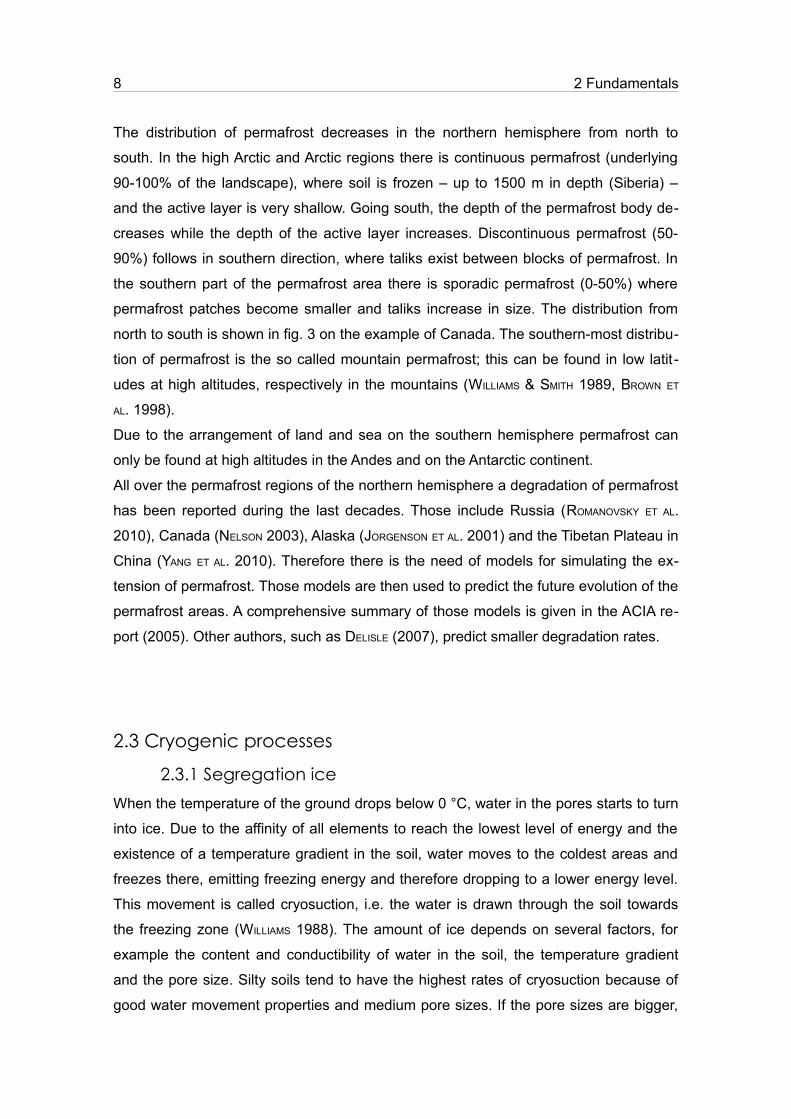
The Lena Delta (72°-74°N, 123°-130°E) is located at the Laptev Sea in the north east-

ern part of the Russian Federation, more precisely in the constituent Yakutian Republic,

Siberia (see fig. 4). The Laptev Sea is part of the Arctic Ocean and the delta forms the

intersection between continent and ocean. The size of about 32 000 km² makes it the

largest delta in the Arctic and one of the largest in the world (GORDEEV & SHEVCHENKO

1995). The north-south stretch is about 150 km and the west-eastern dimension ap-

proximately 230 km. There are more than 1 500 islands in the delta, separated by

channels and branches of different size. The land area of the delta is underlain by per-

mafrost with depth ranging between 500 and 600 m (GRIGORIEV 1960).

Climate

The climate of the Lena Delta can be characterised as high-Arctic and highly continent-

al with low temperatures, due to the high latitude, and low precipitation despite the

closeness of the Arctic Ocean. The low precipitation is mainly caused by the distance

to the Atlantic Ocean and the barriers of the mountains in the south-east of the delta

that shield the Lena Delta from the Pacific Ocean (GÜNTHER 2009). The climate station

in Tiksi, approximately 110 km south-east of the delta on the mainland, records a mean

January temperature of -33.3 °C and +7.0 °C for July (BOIKE ET AL. 2003). The mean an-

nual air temperature during the 30-years-measurement period from 1961 to 1990 is

-13.6 °C (ZUBRZYCKI ET AL. 2008). Total annual precipitation is about 125 mm including

very low winter snowfall with less than 40 mm (BOIKE ET AL. 2003). Snow melt usually

starts in the beginning of June. The snow free period lasts from the middle of June to

mid-September (LANGER 2010) which also represents the growing season. During this

time more or less 45% of the annual precipitation is falling as rain (KUTZBACH 2005).

11

12 3 Study site description

In summer maximum temperatures reach about 20 °C. Polar day lasts from mid-May to

beginning of August. Winter temperatures drop to about -45 °C and the polar night lasts

from mid November to end of January (LANGER 2010).

Fig. 4: Location of the Lena Delta within the Russian Federation and location of the two study sites (source: ESA, RUSSIA MAP).

3.1 The Lena Delta 13

Hydrology

The Lena River has its source in the Baikal

Mountains near the Baikal Lake and is al-

most 4 500 km long before flowing into the

Laptev Sea. The River drains a total area of

2 490 000 km² and is therefore the largest

drainage channel of Siberia. The annual

discharge is 520 km³ of water (LARA ET AL.

1998) and the highest stream flow can be

measured in June (see fig. 5). More than

1/3 of the total annual discharge is released

during this time. This phenomenon is con-

nected to the snow melt in the catchment area (YANG ET AL. 2002). Due to late thawing of

ice in the northern part of the river, ice barriers block the outflow and retain the water.

This leads to oscillations in the water level in the southern parts of the Lena up to 10 m

(GÜNTHER 2009). This event usually occurs during the Lena ice drift in mid-June (LANGER

2010).

There are four major branches flowing through the delta. The largest one is called Tro-

fimovskaya branch and carries about 61% of the total annual water discharge. It is

flowing in eastern direction. The second one, the Bykovskaya branch, transports 25%

of the water in north-eastern direction. The Tumatskaya and the Olenyokskaya branch,

flowing to the north and the west, respectively, both transport about 7% (SCHWAMBORN ET

AL. 2002).

Geology

The geological basement of the Lena Delta is divided in many different units which

form a complex structure. There are many blocks of different height that form the fun-

dament of the delta, overlain by younger river sediments such as sands. In the south-

ern part of the delta the basement can be found at the ground surface whereas it is

buried up to 3 000 m deep beneath sediments in the north-eastern part (GÜNTHER 2009).

The younger sediments level the structure of the basement almost everywhere. Never-

theless there remain open trenches that form some of the big branches through the

delta like the Olenyokskaya branch. On the other hand there are elevations of the

basement such as the Arga Muora Sise (GÜNTHER 2009).

Fig. 5: Mean annual discharge of the Lena near the island of Stolb in the Lena Delta (source: ARCTICNET 2011).

14 3 Study site description

Geomorphology and soils

The Delta of the Lena River is spreading widely due to the northward decreasing tract-

ive force of the river; sedimentation rates are about 21 mio. t a-1 (GÜNTHER 2009).

One can distinguish between 3 different terraces. The first one rises between 1 and

12 m a.s.l. and is covering most of the eastern part of the delta. This youngest terrace

is assumed to form the active part of the delta. The western part, dominated by the

Arga Island, consists of sandy islands with an elevation of 20 to 30 m a.s.l. and repres-

ents the second terrace. The third terrace then rises from 30 to 55 m a.s.l., and is

formed by sandy sequences overlain by an ice complex. This terrace is found in the

southern and south-eastern part of the delta and is the oldest terrace, formed during

the Late Pleistocene (SCHWAMBORN ET AL. 2002).

The area of the Lena Delta was not glaciated during the Quaternary (GALABALA 1997).

Due to rough and cold environmental conditions, the process of soil formation is slow.

The overall production of biomass is low and the produced organic material is mainly

stored in the soil and only partially decomposed by microbes. Typical soil types for the

Lena Delta are, according to the WRB classification, Cryosols (ZUBRZYCKI ET AL. 2008).

Vegetation

Due to the cold environment and the rough wind conditions there are few but highly ad-

apted species of plants. Different kinds of mosses, lichens and herbs are spread on the

drier parts of the islands whereas peat is growing in the wetter areas. Due to high wind

speed shrubs are dwarfish developed (GÜNTHER 2009). According to a vegetation classi-

fication by SCHNEIDER ET AL. (2009: 383) almost 50% of the area of the Lena Delta is

covered with “wet sedge- and moss-dominated tundra”. This includes water saturated

substrates with hydrophilic vegetation (SCHNEIDER ET AL. 2009). This correlates with the

circumpolar Arctic vegetation map developed by WALKER ET AL. (2005) who describes the

vegetation in the Lena Delta mainly consisting of sedges, mosses and dwarf shrub wet-

land.

3.2 Samoylov 15

3.2 Samoylov

Location

The island of Samoylov is located in the upper part of the Lena Delta, at 72°22'N and

126°30'E and covers an area of 4.3 km² (see fig. 4). Nearby is the fork of two of the

main channels of the delta, the Bukovskaya and the Trofimovskaya branch. Fig. 6

shows an aerial picture of Samoylov.

Fig. 6: Aerial picture of Samoylov Island. The first terrace is visible on the right with the typical polygonal ground structure and lakes (source: BOIKE ET AL. 2007).

16 3 Study site description

Geomorphology

The island can be divided into two major units: the floodplain (0 to 4 m a.r.l.) in the

western part (3.4 m²) and a higher-elevated part in the east (1 to 12 m a.r.l., 4.1 m²),

representing the first terrace explained above. The floodplain is overflown with water

from the Lena River annually during the spring flood in June whereas the eastern part

is only flooded during occasional high-water events (ZUBRZYCKI ET AL. 2008).

The first terrace on Samoylov island features a polygonal surface structure that is char-

acteristic for wet tundra landscapes. The polygons have sizes between 25 and 100 m²

and consist of dry, slightly elevated rims and a depression in the centre that is mostly

wet and contains small ponds or water-saturated soils with peat. The rims are between

0.2 and 0.5 m elevated above the centres of the polygons (LANGER 2010). The polygonal

structure is formed by ice wedges that occur beneath the surface of the rims (FRENCH

2007).

Soils

The soil temperatures on the island of Samoylov are very low. The depth of zero annu-

al amplitude of temperatures, which marks the depth were seasonal temperature

changes are not visible any more, occurs approximately at 15 m with temperatures

around -10 °C. During summer time the soil thaws up to a depth between 0.4 and 0.5

m (LANGER 2010).

The western floodplain shows no soil formation and mainly consists of sands. The first

terrace in the eastern part of the island shows a soil pattern following the polygonal sur-

face structure. The soils were formed during the Holocene end experienced no major

disturbances in their development. The wet centres of the polygons consist of gley-

ic-histic cryosols and comprise silty sands with thick accumulations of organic material

under chemically reducing conditions. The porosity of the soil is quite high. The drier

rims consist of gleyic-turbic cryosols and show a silty and/or loamy sand composition

(LUDIN 2010). The organic cover is much thinner on the rims and organic material is un-

der oxic conditions due to the lower water level. The soil structure of the rims is much

more mixed than the one of the polygon centres. Due to cryoturbation processes there

are no stratified layers as there are in the centres (KATTENSTROHT 2009). A more detailed

description of the soils on Samoylov is given in RACHOLD (1999).

Vegetation

About 95% of the islands surface is covered with a moss/lichen layer which grows up to

5 cm height. Only 30% are covered with vascular plants that grow up to 20-30 cm

3.2 Samoylov 17

(KUTZBACH ET AL. 2004: 348). There are differences in vegetation cover between the wet

centres of the polygons and the rims. The centres and the edges of the ponds are

covered with hydrophytic sedges and mosses whereas the rims are dominated by

mesophytic dwarf shrubs, mosses and forbs – only few of the species from the centre

are growing on the rims and the other way round (KUTZBACH ET AL. 2004).

3.3 Kurungnakh

Location

The island of Kurungnakh is located in the southern part of the delta (72°20'N,

126°18'E) close to the Olenyokskaya branch, the major western outflow channel of the

delta (WETTERICH ET AL. 2008). It covers an area of about 330 km² (GÜNTHER 2009). The

location of the island is marked on fig. 4.

Geomorphology

The central part of Kurungnakh is part of the third river terrace, deposited during the

late Quaternary. Some of the boundary sections are part of the first terrace. The island

rises up to 40 m a.r.l. There are two main formations of sediments distinguishable: a

sandy formation and an ice-rich complex that covers the sandy deposits. The Ice Com-

plex, or Yedoma Suite, consists mainly of peat and silt and is frequently interrupted by

thermokarst depressions of different sizes (GÜNTHER 2009). Those depressions are also

called alas (FRENCH 2007).

According to CZUDEK & DEMEK (1970: 103) thermokarst “is the process of melting of the

ground ice accompanied by local collapse of the ground surface and the formation of

depressions”. A disturbance of the thermal equilibrium within the permafrost causes

thermokarst development; this process is shown in fig. 7 using the example of Kurung-

nakh.

The initial state of alas is shown in fig. 7 (1). The landscape is covered with polygonal

tundra and low centre polygons. Then the ice wedges beneath the rims start to thaw,

e.g. by removing the organic layer from the surface, which leads to the development of

high centre polygons. The areas of the former ice wedges are filled with water and start

to affect the surrounding material: by warming the soil, ground ice thaws. The second

stage, fig. 7 (2), shows the thawed polygons and the resulting thermokarst lake. The

material beneath the lake stays unfrozen and is therefore called talik. The process of

18 3 Study site description

thawing the surrounding material continues with time, both vertically and laterally. The

mature state of the thermokarst development is shown in fig. 7 (3). The water-filled de-

pression is as deep as the Ice Complex and the material beneath does not refreeze in

greater depths.

Fig. 7: Thermokarst development in Yedoma landscapes, using the example of Kurungnakh: scheme cross section is on the right, scheme plane view on the left (source: MORGENSTERN ET AL. 2011: 1545).

3.3 Kurungnakh 19

The eroded material from the edges of the lake is deposited at the bottom and is called

taberit. Due to rain events and resulting development of drainage channels the ther-

mokarst drains, sometimes only partially, visible in fig. 7 (4). A small amount of water

remains. The material at the surface refreezes and a second generation of polygonal

tundra is developing. In the fifth stage (fig. 7 (5)) a new ice core beneath the remaining

thermokarst lake results in building up a pingo (GÜNTHER 2009, CZUDEK & DEMEK 1970,

MORGENSTERN ET AL. 2011).

A detailed description of the Ice Complex and the cryostratigraphy on Kurungnakh is

given by WETTERICH ET AL. (2008), MORGENSTERN ET AL. (2011) and SCHIRRMEISTER ET AL.

(2011).

Soils and vegetation

The soils mainly consist of sand as on other islands in the delta and are therefore relat-

ive dry. This leads to sites with xerophytic vegetation, mainly consisting of herbs with

low need for water (KUZMINA & SHER 2006). The uppermost soils are characterised by

SCHIRRMEISTER ET AL. (2010: 7) as “Holocene peaty cryosols”. Within the ice complex

which consists of ice bands and ice veins there are sand and peat lenses. ZUBRZYCKI ET

AL. (2008) refine the soil types to glacic aquiturbels and aquic histurbels.

The soils in the alas depressions were formed during the Pleistocene. Due to the ther-

mokarst development they were compacted. Nowadays these Pleistocene soils are re-

shaped with Holocene soil forming processes (MORGENSTERN ET AL. 2011).

4 Methods

4.1 Field work

4.1.1 Soil samplingExisting methods

There are several ways of taking drilling cores. De-

pending on the intended depth of the core and the ma-

terial that is to be penetrated first choice is between

hand drilling or using technical support in terms of a

motorized drill.

Hand drilling tools are for example the 'Pürckhauer

drill' for short and small cores to a maximum depth of

2 m, especially used for soils with no ice content or

rocks that are easy to penetrate (AG BODEN 2005). As

seen in fig. 8 (A), a straight barre made out of steel is

pushed in the ground by using a sledge and pulled out

with a lever or a drawer. This drill supplies more or

less undisturbed soil samples but due to the size of it

the amount of sample is quite low (ECOTECH). There are

various different drills that can be used by hand and

work more or less in the same way. For penetrating

the ground also twisted drills can be used that have vanes to be screwed into the

ground. For enlarging the depth of the taken cores bore rods can be added to the initial

drill.

A second widely spread method is the use of a motorized drill. There, a drilling rod is

attached to a small engine. This method will be explained more detailed in the follow-

ing.

20

Fig. 8: Pürckhauer drill (A); sledge (B) and lever (C) (source: ECOTECH).

(A)

(B)

(C)

4.1 Field work 21

Used method

For penetrating frozen ground there is a lot of energy necessary. Hand drilling methods

do not work for this reason, the ground is too compact. Due to the ice content the soil is

hard to drill in. Therefore only motorized boring can be used.

Equipment

For drilling into permafrost a robust bore rod with a drilling head is needed. The deeper

the core the longer the rods need to be. Then an engine, normally running with petrol,

is attached to the rod and the core can be taken. Parts of the equipment are shown in

fig. 9.

Previous work

Starting the coring includes the decision of the position of the core. This can be made

before entering the field by using maps and/or satellite images. Anyway it can be ne-

cessary to change the position due to changed surrounding conditions.

It is important to make notes about the whole process of coring to be able to recon-

struct the procedure later. Those notes include, for example, time and position of the

drilling, constitution of the ground, thickness of a possible vegetation cover and the act-

ive layer. The more details available the easier the analysis of the core will be later. It

even might be important to describe the weather conditions during the coring.

Fig. 9: Drilling equipment: (A) engine for penetrating the ground, (B) drilling head with sample (Photo: J. Boike 2009).

(B)(A)

22 4 Methods

Taking the core

When drilling the bore head into the ground and removing it, a core can be taken. Usu-

ally when exploring permafrost the upper, non-frozen part is removed and not part of

the core. Nevertheless this is depending on the research topic.

The drilling head is put on the frozen ground and driven by engine into the soil. Due to

the given size of the bore head only small parts can be removed at one time.

Once the core is exposed to the surface

the next steps need to be made quickly.

Due to the higher temperatures at the

surface the core starts to thaw immedi-

ately and since the diameter of the

drilling equipment is not wide this thaw-

ing affects the whole core. The depth of

the several samples is written down and

then they are packed into sample bags

with description of depth and direction

of the core on them. A sample and its

bag is shown in fig. 10 with the depth

marked on the yellow tape. Then the bags are put into a isolating box to keep them

cold until they can be put into a freezer.

4.1.2 Borehole instrumentationGeneral knowledge

Temperature chains are measuring equipment that are installed to measure several

temperatures over a longer period in a defined interval between the single sensors.

They can be set up for example in water bodies or bore holes. The longer the measure-

ment is set up the more reliable are the temperature values given out. The sensors are

measuring a steady stratification of temperatures with increasing depth in the bore

hole.

In the case of this work two temperature chains had been adjusted in permafrost bore-

holes on the islands of Samoylov and Kurungnakh.

Fig. 10: Sample bag with sample and note of depth and direction of core (Photo: J. Boike 2009).

4.1 Field work 23

Equipment

After drilling the cores a plastic tube is

pushed into the remaining hole with a dia-

meter of 10 cm to have contact with the

surrounding soil material. This tube

matches the length of the bore hole and

finishes with the grounds surface. A

second tube with smaller diameter but

longer dimension is inserted into the first

one. The two tubes – grey and green –

are visible in fig. 11 (A) in the lower part.

In between the two tubes sand or other

soil material is put in for a coupling

between the temperature of the ground

material and the temperature in the tube.

The second tube then is closed at the

bottom so that no water can infiltrate. In

this tube finally the temperature chain is

brought in. The chain contains several

temperature sensors in defined intervals,

depending on depth and desired precise-

ness. The upper most sensor is shown in

fig. 11 (B) and the chain itself in fig. 11 (C). It is important not to cram the chain in the

tube but to reach the bottom exactly. Otherwise the depths of the sensors do not correl-

ate with the depth of the bore hole and it is later impossible to locate the exact depth of

the sensors.

At the end of the chain a data logger collects the data in a time interval that needs to be

specified before by programming the logger. This logger is shown in fig. 11 (D), already

isolated with foam plastic. The isolation is necessary since the logger responses to big

temperature differences in the surrounding atmosphere and so data could be falsified.

After setting the last sensor and the logger the smaller tube is closed at the top to avoid

an infiltration of water. The closure of the tube is shown in fig. 12.

Measuring problems

The Arctic tundra is a very sensitive environment that responds to changes for example

in vegetation cover very quickly. Due to the coring described in the previous chapter

Fig. 11: Installing of temeprature chain with (A) plastic tubes, (B) temperature sensor, (C) temperature chain and (D) the data logger; the red line marks the grounds surface (Photo: J. Boike 2009).

(A)

(B)

(C)

(D)

24 4 Methods

and the installing of the temperature chain on Kurungnakh island a problem showed up

that had not been considered before. As a result of people walking around the bore

hole the vegetation surrounding it had been destroyed. This is visible in fig. 11 where

the area around the bore hole has a darker colour – visible in the foreground – than the

ground further away – in the background. The picture had been taken when installing

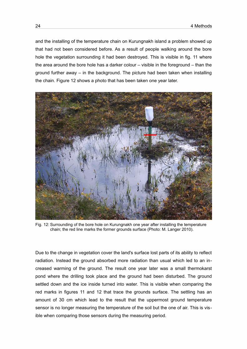
the chain. Figure 12 shows a photo that has been taken one year later.

Due to the change in vegetation cover the land's surface lost parts of its ability to reflect

radiation. Instead the ground absorbed more radiation than usual which led to an in-

creased warming of the ground. The result one year later was a small thermokarst

pond where the drilling took place and the ground had been disturbed. The ground

settled down and the ice inside turned into water. This is visible when comparing the

red marks in figures 11 and 12 that trace the grounds surface. The settling has an

amount of 30 cm which lead to the result that the uppermost ground temperature

sensor is no longer measuring the temperature of the soil but the one of air. This is vis-

ible when comparing those sensors during the measuring period.

Fig. 12: Surrounding of the bore hole on Kurungnakh one year after installing the temperature chain; the red line marks the former grounds surface (Photo: M. Langer 2010).

4.2 Lab measurements 25

4.2 Lab measurements

4.2.1 Importance of measuring the physical properties of the

soilSoil thermal properties are determined by using the composition of the soil and its

structure within the soil column. Those physical properties are determined in the labor-

atory and include the particle size distribution, the ice content and the porosity, the or-

ganic content, the air content and the density.

The particle size distribution influences the ability of the soil to conduct heat just as the

ice, the air and the organic content. Additional the ice content is needed to determine

the volumetric solid content of the soil, which could not be measured itself. This was

not possible due to the irregular shapes of the remaining solid contents after thawing

the sample and the mixing of this content with organic material. If not defined different,

the solid soil content refers here to the mineral content of the soil matrix.

The composition of all soil constituents influences the ability of the soil to store heat, or

the heat capacity, respectively.

4.2.2 The particle size distributionThe particle size distribution had been measured by using a Coulter LS, a laser diffrac-

tion particle size analyzer. It distinguishes different grain sizes by using their different

light diffractions and refractions. The intensity of the detected light after measuring is

analyzed and plotted as the amount of particles in this specific range.

Following grain size ranges had been chosen: clay 0 - <2 µm, silt 2 - <63 µm and sand

>63 µm (AG BODEN 2005). Although the instrument supplies more detailed analysis this

simplified classification meets the needs of the following calculations and is accurate

enough to get an idea about the particle size distribution in the core.

4.2.3 The soil ice content and porosityIce content

The ice content can be calculated by using:

(4.2.1),I=m I

I∗V t

−1

26 4 Methods

with θI being the volumetric ice content as a value between 0 and 1, mI the mass of the

ice content examined by weighting both wet mw and dry mass mds of the sample, and ρI

the density of ice. Vt then is the total volume of the sample.

Porosity

The porosity of the two soil samples is determined by using

(4.2.2),

with φ being the porosity as a number between 0 and 1, and VS the volume of the solid

soil content (including the volume of organic content). The volume of the solid soil con-

tent VS is calculated by subtracting the volume of ice VI and the volume of air VA from

the total volume, which is described in chapter 4.2.5; the following equation shows the

calculation.

(4.2.3)

The volumetric air content θA and therefore the volume of air VA within the sample could

not be measured with the used methods. Therefore it is estimated to be between 0.0

and 0.1. For further calculations a fixed value of θA = 0.05 was used.

4.2.4 The soil organic contentThe procedure of determining the organic content is a standardized lab method

(SCHUMACHER 2002). The sample is weighted and dried. After measuring the weight

again the sample is put in an oven and heated by over 450 °C. At this temperature, the

organic content is burned and after cooling the sample again the weight without the or-

ganic material can be examined. By using the different weights before and after the

heating the organic content can be determined as mass fraction wo of the soil. The or-

ganic weight content is the mass of the soils organic material per total sample weight.

The volumetric organic content θO is evaluated by

(4.2.4),

with mds being the dried mass of solid material of the sample, wO the mass fraction of

=1−V s

V t

V S=V t−V I−V A

O=mds∗wOV t∗O

4.2 Lab measurements 27

organic and ρO the density of organic. In this work the value of FAROUKI (1981b) for the

density of organic (1.3 g cm-³) was used for calculations. The dry mass of the sample

mds had been measured after thawing the frozen block of soil and drying it via freeze

drying.

4.2.5 The soil carbon contentFor calculating the soil organic carbon content (SOCC) the equation given by TARNOCAI

ET AL. (2009) was used:

(4.2.5),

with ρb being the bulk density of the sample, described below, z the layer thickness and

wI the mass fraction of ice.

Since the analysed soil cores do not include the active layer, values from KUTZBACH ET AL.

(2004) for the Samoylov core for the upper 54 cm of the soil were used. Due to the lack

of measurement data, it was not possible to calculate the organic content for the active

layer on Kurungnakh but is was done for the lower soil layers. Therefore the upper

30 cm of the soil of the Kurungnakh core are missing.

4.2.6 The soil densityDefinition of density

The density is given as

(4.2.6),

where ρt is the density of the whole sample (including ice) and mt is the mass of the

sample.

Note that the described soil density differs from the bulk density ρb which is defined as

the dry mass of soil mds per total volume Vt (JURY ET AL. 1991).

Existing methods

There are several ways of measuring the density of soils described in literature. HARTGE

(1988) for example used standardized soil tin cans which is the general method for field

investigations, and is also used by the DECCW (2008). Another way is to cover the

SOCC=wO∗b∗z∗1−w I

t=mtV t

28 4 Methods

sample with paraffin and then dip into a water basin using Archimedes' Principle: a

body dipped in a fluid displaces the same mass of fluid as the body itself possesses. At

the same time the displaced volume correlates with the volume of the body. Because of

the irregular shape of the available drill cores the first method is not adaptive, the con-

tamination of the sample which would take place in the second method makes it also

not usable. However, the general idea of Archimedes Principle of water replacement

had been adopted.

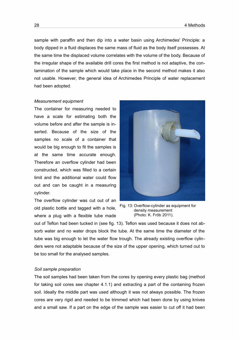
Measurement equipment

The container for measuring needed to

have a scale for estimating both the

volume before and after the sample is in-

serted. Because of the size of the

samples no scale of a container that

would be big enough to fit the samples is

at the same time accurate enough.

Therefore an overflow cylinder had been

constructed, which was filled to a certain

limit and the additional water could flow

out and can be caught in a measuring

cylinder.

The overflow cylinder was cut out of an

old plastic bottle and tagged with a hole,

where a plug with a flexible tube made

out of Teflon had been tucked in (see fig. 13). Teflon was used because it does not ab-

sorb water and no water drops block the tube. At the same time the diameter of the

tube was big enough to let the water flow trough. The already existing overflow cylin-

ders were not adaptable because of the size of the upper opening, which turned out to

be too small for the analysed samples.

Soil sample preparation

The soil samples had been taken from the cores by opening every plastic bag (method

for taking soil cores see chapter 4.1.1) and extracting a part of the containing frozen

soil. Ideally the middle part was used although it was not always possible. The frozen

cores are very rigid and needed to be trimmed which had been done by using knives

and a small saw. If a part on the edge of the sample was easier to cut off it had been

Fig. 13: Overflow-cylinder as equipment for density measurement (Photo: K. Fröb 2011).

4.2 Lab measurements 29

used; due to the frozen condition of the samples the extraction needed to be done

quickly and for further investigations the impact on the rest of the sample had to be as

small as possible. Using the saw for example started to melt small parts of the core due

to frictional heat.

Note that the applied method is destructive to the sample.

Density measurement

For measuring the density the samples had been weighted in frozen condition, giving

the wet mass mw of the sample, then weld in thin foil, weighted again, giving out mwf,

and brought in the described overflow cylinder. The foil is necessary because of the

avoidance of contaminating the sample. Because of the possible error according to the

foil and the included air the whole sample had been vacuum-packed by using a vacu-

um pump. The overflowing water from the cylinder had been caught in a measuring cyl-

inder and the volume was read out, giving Vt as value for every sample. The weight of

the foil mf had been examined by subtracting mw from mwf and was used later to exam-

ine the dried sample mass mds.

It was important to keep the samples under frozen condition. Therefore the measure-

ments were performed in a cooling chamber at approximately 4 °C and only a few

samples were taken out of the freezer at one time so that the samples did not have

enough time to melt completely although the edges were affected. The water in the

overflow cylinder was held at temperature around 0 °C. Outflow disturbance due to sur-

face tension was avoided by adding a little bit of dish liquid to the water so that the wa-

ter drained exactly at the edge of the Teflon tube.

Furthermore, the temperature dependence of the water density was accounted for in

the measurements.

Possible sources of error

The obtained density values are subject to measurement errors, including both the

mass and the volume determination. However, the combined error on the density is

less than 1% assuming Gaussian error propagation. Consequently, the density error af-

fects the calculations on the soil constituents.

Further errors are induced by the foil around the sample whose volume has not been

taken into account nor the potential shortcomings in the vacuum between foil and

sample. Those errors are difficult to quantify but assumed to be below the accuracy as

determined above. Added to this the heterogeneity in the soil and therefore the uncer-

tainties of values are much higher than the mathematical error.

30 4 Methods

It needs to be considered that the variations in the core itself are higher than those cal-

culated. Therefore a detection of density distribution with depth is possible, although

variations are not significant.

4.3 Determination of soil thermal properties

4.3.1 The volumetric and specific heat capacityThe soil volumetric heat capacity cv is the sum of the volumetric heat capacities of the

single components cv,n occurring in the soil weighted by their volumetric content θn. The

subscript n always refers to the several soil components:

(4.3.1).

The subscripts O, I, S and A refer to components of organic, ice, solid material and air.

The volumetric heat capacities used in this work are given in table 1. They have been

calculated by using:

(4.3.2),

with ρn being the density of the soil constituent and ch,n its specific heat capacity.

4.3.2 The thermal conductivity from soil temperature data

(Conduction method)The conduction method was developed by WESTERMANN ET AL. (2009) and also used by

LANGER (2010). It directly calculates the thermal diffusivity of a soil column which can be

used in combination with the above described heat capacity to estimate the soils

thermal conductivity.

By assuming a conductive 1-D-heat transport temperature changes are governed by

the heat transfer equation as:

(4.3.3).ch z , t ∂∂ tT z , t = ∂

∂ zK ht , z ∂

∂ zT t , z

cv=O cv ,OI cv , IS cv , SA cv , A

cv , n=n∗ch , n

4.3 Determination of soil thermal properties 31

By taking the specific heat capacity ch and the heat conductivity Kh as constant in

space equation (4.3.3) can be expressed as

(4.3.4),

with

(4.3.5)

being the thermal diffusivity dh of the soil column. For computation the thermal diffusiv-

ity three time series of temperature in a profile of different depths are needed. They

may be called Tmeas(z1, t), Tmeas(z2, t) and Tmeas(z3, t) with z being denoted as depth of the

sensor and z1 < z2 < z3. The boundary conditions for solving equation (4.3.3) are given

by the two time series Tmeas(z1, t) and Tmeas(z3, t). The heat capacity and the thermal

conductivity are considered to be equal for every calculated part of the soil.

The initial condition for solving the equation is assumed to be a linear interpolation

between the two outer sensors, respectively the boundary conditions of Tmeas(z1, t=0)

and Tmeas(z3, t=0). It is not necessary for the initial condition to be highly exact due to

the fact that after a few time steps calculated values are getting independent from it.

The numerical solution of equation (4.3.4) is performed in MATLAB and gives the

modeled temperature distribution through the considered soil layer, including the

middle temperature value Tmod(z2, t).

It is important to exclude the time series, where phase change occurs, i.e. from water

to ice or other way round, because equation (4.3.4) does not account for it (LANGER

2010b; WESTERMANN ET AL. 2009).

The model gives the thermal diffusivity dh as output. By using equation (4.3.4) with

physical properties such as volumetric contents of the different soil components the

thermal conductivity can be calculated with equation (4.3.5).

A least-mean-square fit for dh can be performed by using Tmeas(z2, t). Thereto the RMS

error between Tmeas(z2, t) and Tmod(z2, t) is minimized.

∂∂ tT (z , t)=d h

∂2

∂ z2 T (z ,t )

d h=Khch

32 4 Methods

4.4 Modeling of thermal conductivity

4.4.1 Calculating the soil thermal conductivity using the de

Vries method (1952)The first of the presented methods for calculating the thermal conductivity of soils as a

porous medium is the theory developed by de Vries (1952). The soil consists of volu-

metric fractions of water, air and a solid matrix, which again is subdivided in a solid,

e.g. sand and/or clay, and an organic fraction (WESTERMANN 2010; DE VRIES 1975). Soil

volume is considered much larger than the soil grains so that micro-scale heterogeneit-

ies average out. For simplification reasons the particles of the solid matrix are assumed

to have spherical shape (DE VRIES 1975).

De Vries (1951) developed his model for a water-air system, i.e. the pores are filled

either with water or air or both. In the present work there had been a generalization

from water-air systems to air-ice systems. In the now applied system the pores within

the soil are filled with either air or ice or both. The outcome of this are interfaces

between air and ice. The same input parameters as for the water-air system then had

been adapted to the air-ice system. This adaption was also successfully done by IPPISCH

(2001).

To calculate the thermal conductivity of the described unit cell, the thermal conductivity

of every fraction in combination with the volumetric amount of the fraction and a weight-

ing factor was used. Equation (4.4.1) describes the computation:

(4.4.1),

with Kh,n being the thermal conductivity of the soil components, e.g. solid, ice, water or

organic material, and θn being the volumetric content of the fraction. The weighting

factor fn describes the dimension of the impact of the fraction (DE VRIES 1975;

WESTERMANN 2010). These are defined in the laboratory as described in the previous

chapter 4.2. The conductivities for the pure components are available in literature, al-

though having partially big ranges. Table 1 shows the employed values for all calcula-

tions:

K h=n f nnK h , n

n f nn

4.4 Modeling of thermal conductivity 33

Table 1: Thermal properties of soil components (taken from: FAROUKI 1981b: 12)

soil component thermal conductivityKh [W m-1 K-1 ]

volumetric heat capacity cV [MJ m-³ K-1]

solid mineral 2.9 2.4organic 0.3 2.3

air 0.025 9.26*10-4

ice 2.2 2.0

The weighting factor fn controls the influence of the different fractions and is calculated

as followed:

(4.4.2)

with Kc being the thermal conductivity of the continuous phase, which connects the sev-

eral fractions of the soil. This continuous phase is therefore important to define (FAROUKI

1981b; WESTERMANN 2010). As the soil particles are assumed to be spherical, only water,

ice or air can form the mentioned phase. By taking a transition from air-filled to ice-filled

pores into consideration, one must define Kc as

(4.4.3)

with

(4.4.4).

Kh,a and Kh,i refer to the conductivities of air and ice, βai is the transition parameter, θi

being the volumetric ice content and θi0 a soil parameter related to the ice content in

the soil, where ice “starts to affect thermal conductivity” (CAMPBELL ET AL. 1994: 308). εs is

a smoothing parameter (WESTERMANN 2010). For both variables θi0 and εs there are val-

ues given by CAMPBELL ET AL. (1994) for different soils; in this thesis θi0 = 0.15 which can

be assumed for the soils found in the study area and is also used by WESTERMANN

(2010). The smoothing parameter εs is set to 4.

Zero unfrozen water content had been assumed which is reasonable for the temperat-

ure encountered at the study site.

f n=[113K h , n

K c−1]

−1

K c=K h , aai K h ,i−K h , a

ai=[1ii0

−s

]−1

34 4 Methods

4.3.2 The Johansen model (1975)The second method presented in this work is the modeling theory of Johansen (1975),

shown in FAROUKI (1981b). The theory is based on the different composition of grain

sizes in the soil, combined with the amount of organic. The grain sizes and their

amount had been determined in the lab, described in chapter 4.2.2, just as the organic

content, reported in chapter 4.2.4.

In the following equations only values were put in without units.

The Johansen calculation is based on “a combination of the dry Kdry and saturated Ksat

thermal conductivity weighted by a normalized thermal conductivity” (LAWRENCE & SLATER

2006: 148), called the Kersten number, Ke. The two conductivities are depending on the

soil type, especially on the grain size distribution and the organic material. For calcula-

tion the thermal conductivity Kh after Johansen's equation is used as followed:

(4.4.5).

The organic fraction fsc for every soil layer is defined as

(4.4.6),

with ρsc being the soil carbon density and ρsc,max = 1.3 g cm-³ the maximum carbon

density, given by LAWRENCE & SLATER (2006). Next, the volumetric ice content is calcu-

lated for the mineral soil, θsat, min, by using

(4.4.7);

the volumetric sand content is needed for calculation. The sand content refers to the

percentage of grain size fraction and shall not be mistaken by using the volumetric

sand content referring to the whole sample. Since equation (4.4.7) only refers to miner-

al content, the organic part of the soil is included with

(4.4.8)

by assuming θsat,sc = 0.9 [-] (LAWRENCE & SLATER 2006). The dry mineral conductivity

Kdry,min is now calculated following JOHANSEN (1975):

(4.4.9).

f sc=sc

sc , max

sat , min=0.489−0.00126 % sand

sat=1− f sc sat , min f scsat , sc

K h=K eK sat1−K eK dry

K dry , min=0.135b64,72700−0.947b

4.4 Modeling of thermal conductivity 35

The term ρb is the bulk density of the mineral soil and has to be calculated here with

(4.4.10).

In combination with the calculated thermal conductivity of dry organic soils Kdry,sc =

0.1 W m-1 K-1, performed by FAROUKI (1981b) and given by LAWRENCE & SLATER (2006) the

dry thermal conductivity of the soil column can be calculated with

(4.4.11).

The saturated thermal conductivity on the other hand is given by

(4.4.12)

with Kliq being the thermal conductivity of liquid water and Kh,i the conductivity of ice. θliq

is the volumetric liquid water content, which is assumed to be zero in the present work.

Therefore Ks, the soil solid thermal conductivity, can be described as

(4.4.13),

while defining Kh,o = 0.25 W m-1 K-1 as the organic solid soil conductivity after LAWRENCE

& SLATER (2006). The conductivity of the mineral part of the soil column Ks,min is ex-

pressed as

(4.4.14).

As it was shown, the method by Johansen is based on the grain size distribution and

the volumetric organic content in the soil.

4.3.3 Conductivity after Endrizzi et al. (2011)The last of the presented modeling methods here is the calculation of conductivities

performed by ENDRIZZI ET AL. (2011). They used a simple equation to calculate the soil

thermal conductivity Kh which on the other hand is adaptable to frozen soils. The follow-

ing equation shows the computation

(4.4.15).K h= nK h , n2

b=27001−sat , min

K dry=1− f scK dry , min f sc K dry , sc

K sat=K s1− sat K liq

sat K h , isat−liq

K s=1− f scK s ,min f scK h , o

K s , min=8.8 % sand 2.92 %clay

%sand %clay

36 4 Methods

The different constituents, presented by the subscript n, are “solid soil, liquid water, ice,

air” (ENDRIZZI ET AL. 2011: 375f.). The thermal heat conduction of the different soil com-

ponents is given in table 1.

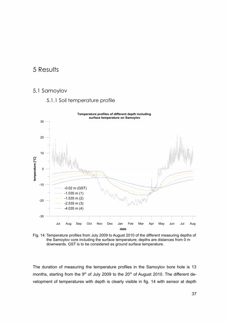
5 Results

5.1 Samoylov

5.1.1 Soil temperature profile

The duration of measuring the temperature profiles in the Samoylov bore hole is 13

months, starting from the 9th of July 2009 to the 20th of August 2010. The different de-

velopment of temperatures with depth is clearly visible in fig. 14 with sensor at depth

37

Fig. 14: Temperature profiles from July 2009 to August 2010 of the different measuring depths of the Samoylov core including the surface temperature; depths are distances from 0 m downwards. GST is to be considered as ground surface temperature.

Jul Sep Nov Jan Mar May JulAug Oct Dec Feb Apr Jun Aug

date

-30

-20

-10

0

10

20

30

tem

pera

ture

[°C

]

-0.02 m (GST)-1.035 m (1)-1.535 m (2)-2.535 m (3)-4.035 m (4)

Temperature profiles of different depth including surface temperature on Samoylov

38 5 Results

(1) as the shallowest sensor having the largest amplitude and the sensor at depth (4)

the smallest. With increasing depth a temperature signal is smoothed and needs more

time to travel, therefore deviations showsup later the deeper the temperature sensor is

located. The phase shifting between the sensors is noticeable; the maxima and minima

in temperature are experiencing a time shift with increasing depth, as visible in the

maxima of sensor at depth (1) during late November 2009 and the one from the sensor

at depth (4) one month later. At those extreme points the gap between the several tem-

perature sequences gets smaller with depth, e.g. the minimum in winter, where the dif-

ference between sensor at depth (1) and (3) accounts for 6 K whereas it is 3.5 K

between sensor (3) and (4). Accordingly sensor (1) shows an deviation from the sinus-

oidal course during the second week of November 2009, which is also in a smaller

scale visible in the deeper sensors at depth (2), (3) and (4) when enlarging fig. 14. This

is related to a temporary increase in temperatures at the surface as recognizable when

comparing the GST to those graphs. A second irregularity in GST is found during early

February 2010 which again creates a signal also recorded by the deeper sensors.

The freeze back, i.e. the re-freezing of the soil in autumn where soil temperatures near

to the surface drop beneath 0 °C, occurs from the last week of September until the be-

ginning of October, more or less 10 days long. This is visible in the temperature step of

the GST during that time where values are slightely under 0 °C. The thawing period

lasts from 10th May to 7th June where data of GST balance around 0 °C after a steep in-

crease of temperature on 9th May, where data jump up from -10 °C to -2 °C on 10th May.

In the following GST shows an abrupt rise to values above 0 °C.

5.1.2 Soil physical propertiesThe Samoylov core shows no major variations with depth in all physical properties. The

detected maxima and minima are nearly all within the range of uncertainty. A short de-

scription of the developing of values for the several properties is given in the following.

The grain size distribution shows the following characteristics: the clay content, that

was detected in the Samoylov core, is not significantly changing with depth; values

range more or less around 5% and are overall low. The biggest fraction is the silt con-

tent with values ranking between 37 and 76%. The highest variations are found in the

sand content with 18 to 60%. There is no trend with depth visible except the increase in

variability.

The curve of the total organic content (TOC) shows, after a small minimum, a steep

5.1 Samoylov 39

increase of values which result in a peak at 140 cm depth with an organic content of

2.9 vol.%. This is the highest rate within the core. After that values drop quickly to

0.6 vol.% at 170 cm depth followed by a second but lower peak at 250 cm (2.0 vol.%)

and a second decrease as far as 0.7 vol.%. Subsequently values for the TOC settle

around 1.4 vol.% with small variations.

The porosity of the Samoylov core shows increasing values until depth 200 cm, fol-

lowed by a decrease as far as depth 310 cm and a new slight increase. Data start from

~60 vol.% porosity, reach ~80 vol.% at maximum, drop to ~50 vol.% and rise again to

~70 vol.%.

The curve of the ice content follows the porosity exactly as nearly all pores are filled

with ice (see chapter 4.2.3). The offset between the two curves is the air content in the

pores. The values of the ice content increase until depth of 200 cm to a maximum of

73 vol.% of ice content in the core. With increasing depth variations become more sig-

nificant.

The curve of the density trend shows a quite regular development. Values are relat-

ively low, more precisely around 1.0 g cm-³, and therefore just about the density of ice.

The values of the density are not significantly increasing with depth. There is no well-

defined correlation to the grain size contribution. The small variations in density are

caused by multiple factors, such as ice and organic content.

Fig. 15: Physical properties of the Samoylov core.

0 20 40 60 80 100

grain size fraction [%]

0 1 2 3 4

TOC [vol.%]

0 20 40 60 80 100

porosity [vol.%]

0 20 40 60 80 100

ice content [vol.%]

0 0.5 1 1.5 2

density [g cm-³]

400

300

200

100

0

dept

h [c

m]

<2 µm

2 - <63 µm

>63 µm

40 5 Results

5.1.3 Calculation of conductivity

Conduction method

The conduction method provides data with small variations. The volumetric heat capa-

city, that is needed for calculation, is shown in fig. 16 a. Values are slightly over

2.0 MJ m-3 K-1 which is close to the heat capacity for ice.

The conductivity itself provides data just below 2.0 W m-1 K-1. As there are two different

diffusivities given for different depths by the model, the one with clearer minimum in

terms of diffusivity had been chosen for calculating the thermal conductivity. Results

are shown in fig. 17. There were four temperature sensors available in the Samoylov

core that match the restriction of not crossing the 0 °C limitation. That is why diffusivit-

ies for two depths can be provided, shown in fig. 17 A.

As visible in fig. 17 B the mean diffusivity between sensor at depth two and four shows

a clearer minimum. Therefore the correlation between the interpolated and the real

measured data is better. That is the reason for choosing this output diffusivity as con-

stant for the whole core. The two obtained diffusivities were 8.6*10-7 m² s-1 for the depth

between sensor one and three and 9.6*10-7 m² s-1 for the depth between sensor two

and four.

Fig. 16: Thermal properties for the Samoylov core calculated by using different models.

1.5 2 2.5

volumetric heat capacity [MJ m-³ K-1]

400

300

200

100

0

dept

h [c

m]

1 1.5 2 2.5 3

conductivity after Johansen (1977)

[W m-1 K-1]1 1.5 2 2.5 3

conductivityafter de Vries (1952)

[W m-1 K-1]1 1.5 2 2.5 3

conductivityafter Endrizzi (2011)

[W m-1 K-1]1 1.5 2 2.5 3

conductivityconduction method

[W m-1 K-1]

a b c d e

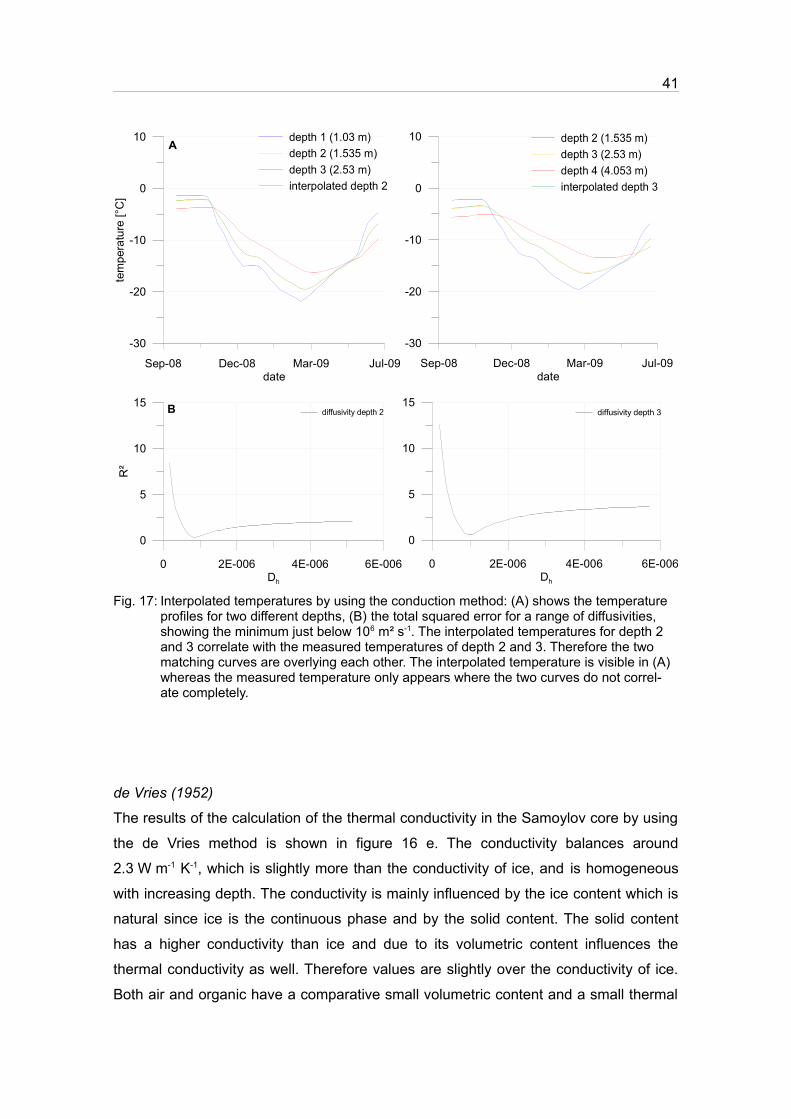
41

de Vries (1952)

The results of the calculation of the thermal conductivity in the Samoylov core by using

the de Vries method is shown in figure 16 e. The conductivity balances around

2.3 W m-1 K-1, which is slightly more than the conductivity of ice, and is homogeneous

with increasing depth. The conductivity is mainly influenced by the ice content which is

natural since ice is the continuous phase and by the solid content. The solid content

has a higher conductivity than ice and due to its volumetric content influences the

thermal conductivity as well. Therefore values are slightly over the conductivity of ice.

Both air and organic have a comparative small volumetric content and a small thermal

Fig. 17: Interpolated temperatures by using the conduction method: (A) shows the temperature profiles for two different depths, (B) the total squared error for a range of diffusivities, showing the minimum just below 106 m² s-1. The interpolated temperatures for depth 2 and 3 correlate with the measured temperatures of depth 2 and 3. Therefore the two matching curves are overlying each other. The interpolated temperature is visible in (A) whereas the measured temperature only appears where the two curves do not correl-ate completely.

0 2E-006 4E-006 6E-006Dh

0

5

10

15

R²

diffusivity depth 2

0 2E-006 4E-006 6E-006Dh

0

5

10

15diffusivity depth 3

Sep-08 Dec-08 Mar-09 Jul-09date

-30

-20

-10

0

10te

mpe

ratu

re [°

C]

depth 1 (1.03 m)depth 2 (1.535 m)depth 3 (2.53 m)interpolated depth 2

Sep-08 Dec-08 Mar-09 Jul-09date

-30

-20

-10

0

10 depth 2 (1.535 m)depth 3 (2.53 m)depth 4 (4.053 m)interpolated depth 3

A

B

42 5 Results

conductivity; their influence on the thermal conductivity is negligible.

Johansen (1975)

The curve of the thermal conductivity calculated with the Johansen method shows high

variations. Values are shown in figure 16 c. Data range from 1.2 to 2.7 W m -1 K-1 and

there is no clear trend visible. The variations are driven by the organic content in the

core. The higher the content of organic the smaller the thermal conductivity gets. A

minor role in terms of influencing the thermal conductivity is played by the grain size

distribution. Although being necessary for calculation there is no clear connection

between conductivity and sand and/or clay content visible.

Endrizzi et al. (2011)

The development of the thermal conductivity calculated by using the method developed

by Endrizzi et al. (2011) shows a similar development as the curve of the de Vries

method although having an offset. Values are shown in fig. 16 d. This offset is on the

order of 0.2 W m-1 K-1; the conductivity calculated by de Vries is slightly higher. The val-

ues are around 2.2 W m-1 K-1 which is just about the thermal conductivity for ice.

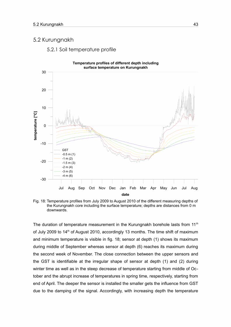
5.2 Kurungnakh 43

5.2 Kurungnakh

5.2.1 Soil temperature profile

The duration of temperature measurement in the Kurungnakh borehole lasts from 11 th

of July 2009 to 14th of August 2010, accordingly 13 months. The time shift of maximum

and minimum temperature is visible in fig. 18; sensor at depth (1) shows its maximum

during middle of September whereas sensor at depth (6) reaches its maximum during

the second week of November. The close connection between the upper sensors and

the GST is identifiable at the irregular shape of sensor at depth (1) and (2) during

winter time as well as in the steep decrease of temperature starting from middle of Oc-

tober and the abrupt increase of temperatures in spring time, respectively, starting from

end of April. The deeper the sensor is installed the smaller gets the influence from GST

due to the damping of the signal. Accordingly, with increasing depth the temperature

Fig. 18: Temperature profiles from July 2009 to August 2010 of the different measuring depths of the Kurungnakh core including the surface temperature; depths are distances from 0 m downwards.

Jul Sep Nov Jan Mar May JulAug Oct Dec Feb Apr Jun Aug

date

-30

-20

-10

0

10

20

30

tem

pera

ture

[°C

]

GST-0.5 m (1)-1 m (2)-1.5 m (3)-2 m (4)-3 m (5)-4 m (6)

Temperature profiles of different depth includingsurface temperature on Kurungnakh

44 5 Results

signal needs more time to travel.

Both GST and sensor at depth (1) show a huge difference in the two summers. In sum-

mer 2009 GST ranged between 0 and 10.0 °C and sensor (1) barely exceeds 0 °C. The

summer of 2010, in comparison, shows GST ranging from 2.0 to more than 20 °C and

the sensor at depth (1) passes the 0 °C boundary widely while possibly not even cul-

minate maximum summer temperatures. Those changes are mainly caused by the dif-

ferent environmental conditions in the two consecutive years. The vegetation cover

around the instrumented bore hole had been destroyed and so the ground settled

down. Therefore the sensor at depth (1) did not measure ground but surface temperat-

ures (further explanation in chapter 4.1.2).

The freeze back takes place during the last week of September and the first week of

October. Values of the GST are ranking between -1.8 °C and +1.0 °C and the sensor at

depth (1) experiences a slow decrease in temperatures from -0.1 °C to -0.3 °C. After

this step GST is dropping down faster whereas sensor (1) keeps decreasing slowly and

shows its bend during the third week of October; the other sensors follow with time.

The thawing period can be identified from 19th May to 9th June where data show a

steep increase from -6.0 °C to almost 0 °C. In the following values range around 0 °C

until the 9th June where an abrupt rise in temperature is visible.

5.2.2 Soil physical properties

Fig. 19: Physical properties of the Kurungnakh core.

0 0.5 1 1.5 2

bulk density [g cm-³]

400

300

200

100

0

dept

h [c

m]

0 20 40 60 80 100

ice content [vol.%]

0 20 40 60 80 100

porosity [vol.%]

0 1 2 3 4

TOC [vol.%]

0 20 40 60 80 100

grain size fraction [%]

<2 µm

>63 µm

2 - <63 µm

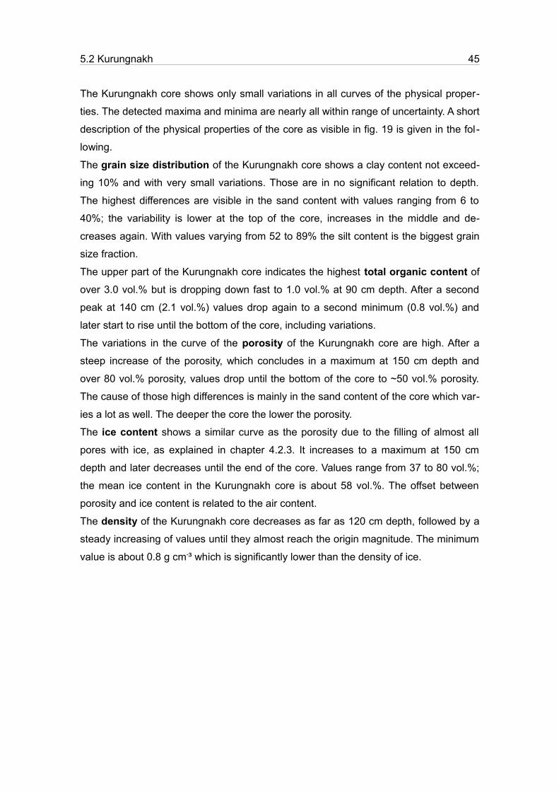
5.2 Kurungnakh 45

The Kurungnakh core shows only small variations in all curves of the physical proper-

ties. The detected maxima and minima are nearly all within range of uncertainty. A short

description of the physical properties of the core as visible in fig. 19 is given in the fol-

lowing.

The grain size distribution of the Kurungnakh core shows a clay content not exceed-

ing 10% and with very small variations. Those are in no significant relation to depth.

The highest differences are visible in the sand content with values ranging from 6 to

40%; the variability is lower at the top of the core, increases in the middle and de-

creases again. With values varying from 52 to 89% the silt content is the biggest grain

size fraction.

The upper part of the Kurungnakh core indicates the highest total organic content of

over 3.0 vol.% but is dropping down fast to 1.0 vol.% at 90 cm depth. After a second

peak at 140 cm (2.1 vol.%) values drop again to a second minimum (0.8 vol.%) and

later start to rise until the bottom of the core, including variations.

The variations in the curve of the porosity of the Kurungnakh core are high. After a

steep increase of the porosity, which concludes in a maximum at 150 cm depth and

over 80 vol.% porosity, values drop until the bottom of the core to ~50 vol.% porosity.

The cause of those high differences is mainly in the sand content of the core which var-

ies a lot as well. The deeper the core the lower the porosity.

The ice content shows a similar curve as the porosity due to the filling of almost all

pores with ice, as explained in chapter 4.2.3. It increases to a maximum at 150 cm

depth and later decreases until the end of the core. Values range from 37 to 80 vol.%;

the mean ice content in the Kurungnakh core is about 58 vol.%. The offset between

porosity and ice content is related to the air content.

The density of the Kurungnakh core decreases as far as 120 cm depth, followed by a

steady increasing of values until they almost reach the origin magnitude. The minimum

value is about 0.8 g cm-³ which is significantly lower than the density of ice.

46 5 Results

5.2.3 Calculation of conductivity

Conduction method

The curve for the conduction method calculating the thermal conductivity shows the

smallest variations, visible in fig. 20 b. The volumetric heat capacity, that is needed for

calculation, has been plotted in fig. 20 a. The two curves show similarity in develop-

ment with the heat capacity having greater variations. The mean conductivity for the

whole core is about 2.2 W m-1 K-1 and the mean heat capacity ranges around 2.1 MJ m-

³ K-1. There were three different diffusivities available since five depths for interpolating

could be used. Depth 1 needed to be excluded because of the phase change of water

in this depth. This phase change is visible in fig. 18 where temperatures pass the 0 °C

limitation. The interpolations that were possible are shown in fig. 21 A and the corres-

ponding correlation coefficients in fig. 21 B.

The three given diffusivities were 8.0*10-7 m² s-1 for the depth between sensor two and

four, 1.1*10-6 m² s-1 for the depth between sensor three and five and 8.6*10-7 m² s-1 for

the depth between sensor four and six. Because showing the clearest minimum the dif-

fusivity between sensor at depth three and five had been chosen for calculation.

Fig. 20: Thermal properties for the Kurungnakh core calculated by using different models.

1.5 2 2.5

volumetric heat capacity [MJ m-³ K-1]

400

300

200

100

0

dept

h [c

m]

1 1.5 2 2.5 3

conductivity after Johansen (1977)

[W m-1 K-1]1 1.5 2 2.5 3

conductivityafter de Vries (1952)

[W m-1 K-1]1 1.5 2 2.5 3

conductivityafter Endrizzi (2011)

[W m-1 K-1]1 1.5 2 2.5 3

conductivityconduction method

[W m-1 K-1]

a b c d e

5.2 Kurungnakh 47

de Vries (1952)

The calculation for soil thermal conductivity after the de Vries method is shown in fig.

20 e. After a small decrease in values until 150 cm depth data increase slowly until the

bottom of the core. The minimum has a magnitude of 2.1 W m-1 K-1 and correlates with

a maximum in porosity. This can be explained by the differences in the thermal con-

ductivity of the soil components: the solid content has a high conductivity and ice a

smaller one (for values see table 1). Since the porosity is high at the depth of the min-

imum there is more ice in the layer than minerals. Therefore the conductivity is lower.

The mean conductivity is 2.3 W m-1 K-1 for the whole core and therefore only little over

the conductivity for ice. This value was expected since ice has by far the highest volu-

metric content in the core and the second biggest fraction, the solid content, possesses

a higher conductivity.

Fig. 21: Interpolated temperatures of the Kurungnakh core by using the conduction method: (A) shows the temperature profiles for two different depths, (B) the total squared error for a range of diffusivities, showing the minimum just below 106 m² s-1. The interpolated tem-peratures for depth 3, 4 and 5 correlate with the measured temperatures of depth 3, 4 and 5. Therefore the two matching curves are overlying each other. The interpolated temperature is visible in (A) whereas the measured temperature appears where the two curves do not correlate completely.

Jun-09 Nov-09 Apr-10 Sep-10date

-30

-20

-10

0

10

tem

pera

ture

[°C

]

depth 2 (1m)depth 3 (1.5 m)depth 4 (2 m)interpolated depth 3

Jun-09 Nov-09 Apr-10 Sep-10date

-30

-20

-10

0

10 depth 3 (1.5 m)depth 4 (2 m)depth 5 (3 m)interpolated depth 4

Jun-09 Nov-09 Apr-10 Sep-10date

-30

-20

-10

0

10 depth 4 (2 m)depth 5 (3 m)depth 6 (4 m)interpolated depth 5

0 2E-006 4E-006 6E-006dh

0

5

10

R²

diffusivity depth 3

0 2E-006 4E-006 6E-006 8E-006dh

0

5

10diffusivity depth 4

0 2E-006 4E-006 6E-006dh

0

5

10diffusivity depth 5

A

B

48 5 Results

Johansen (1975)

The soil thermal conductivity calculated by using the Johansen method shows very

high variations for the Kurungnakh core. This is visible in fig. 20 c. The highest vari-

ations are concentrated in the middle of the core between 150 and 300 cm depth.

There, data oscillate between 2.5 and 3.0 W m-1 K-1. They are mainly influenced by the

organic content and, in a smaller scale, the sand fraction of the core. In comparison to

other models values for the thermal conductivity are high which is surprising since the

organic content, that influences the thermal conductivity most, possesses only a small

thermal conductivity.

Endrizzi et al. (2011)

The conductivity of the soil calculated with the method developed by Endrizzi et al.

(2011) shows a similar trend as the curve of the de Vries calculation. The mean thermal

conductivity is 2.2 W m-1 K-1 which is just about the conductivity for ice. There are only

minor variations, shown in fig. 20 d.

5.3 Comparison

5.3.1 Soil temperature profilesThe comparison of the two temperature profiles of Samoylov and Kurungnakh shows

that there are some differences. The freeze back at the surface occurs at the same

time although Kurungnakh “needs” a little bit longer. The time is around last week of

September and beginning of October. The thawing period shows more differences. On

Samoylov thawing starts on 9th May very abruptly and data range around 0 °C after a

small minimum on 14th May. On Kurungnakh thawing begins on 19th May, ergo 10 days

later, and the development of temperatures is neither as steep as on Samoylov nor as

high as there; it looks more step-like.

5.3.2 Soil physical propertiesThe two cores of Samoylov and Kurungnakh do not differ significantly in the analysed

physical properties. Due to the uncertainties of the measuring methods the identified

results of the soil cores are all within the same range. They are very similar in all prop-

erties and do not show a clear trend with depth. This is surprising since the soils have

5.3 Comparison 49

quite different evolutionary histories.

The grain size distribution of the soil cores showed the following deviations when

compared to each other: the clay content of the Kurungnakh core is about twice as high

as the one from Samoylov but having the same, small variations in depth. Although the

deviation seems quite high the overall clay content is still low. The two soil cores have

a big silt fraction in common, which is again higher in the Kurungnakh core. The Sam-

oylov core contains the bigger sand content with the higher variability.

Both TOC-curves display a maximum at 140 cm depth and a second, smaller one

between 240 and 250 cm. In the upper parts of the core, Samoylov possesses the

higher values of organic content. The overall organic content is not high; Samoylov

contains in average 1.5 vol.% organic and Kurungnakh 1.4 vol.% which again shows

the similarity of the two cores.

The porosity-curves of the two soil cores show a similar trend of rising to a maximum

in depth between 150 and 200 cm and a followed decrease of values. The overall

porosity is quite high: Samoylov on average 63 vol.% and Kurungnakh 58 vol.%. The

difference is mainly caused by a higher sand fraction in the Samoylov core.

The development of the ice content with increasing depth is similar in both soil cores.

After a maximum between 150 and 200 cm depth values are decreasing, in case of

Kurungnakh until the bottom. The Samoylov core shows an increase in values from

300 cm depth until the bottom which can be explained by the high sand content in this

part of the core.

The two curves do not show any similarity in density. This is caused by the strong in-

fluence of many factors that control this property, e.g. the ice content, the sand and

clay content or the organic content.

5.3.3 Calculation of conductivityConduction method

The curves of the thermal conductivity calculated by using the conduction method for

the soil cores from Samoylov and Kurungnakh both show only minor variations. The

conductivity of the Samoylov core balances around 2.0 W m-1 K-1 whereas mean value

is about 2.2 W m-1 K-1 in the Kurungnakh core. This offset can be explained by the dif-

ference in the heat capacity of the two soil cores which have nearly the same values of

2.0 and 2.2 W m-1 K-1. In the Kurungnakh core there is a slight increase in values visible

with ongoing depth whereas the Samoylov core does not show anything alike.

50 5 Results

de Vries (1952)

The overall development of the thermal conductivity with depth calculated with the de

Vries method is similar in both cores. From the top there is a slight decrease that res-

ults in a small minimum. This minimum can be found at 200 cm depth in the Samoylov

core and at 150 cm in the Kurungnakh core. Both conductivities are in the range

between 2.0 and 2.5 W m-1 K-1, although variations are higher in the Kurungnakh core.

Both cores reach their initial conductivity at their bottom again.

Johansen (1975)

The two curves of the two soil cores calculated with the Johansen method look com-

pletely different to each other. The Samoylov core shows small values for the central

part of the core whereas the Kurungnakh core shows quite high conductivities for this

part. A small similarity can be seen in the lower part of the core, starting from 375 cm

depth. After a maximum at that depth values drop down and rise again until the bottom

of the core. Although having different magnitudes and lengths the development looks

similar.

Endrizzi et al. (2011)

The conductivities of both cores calculated by using the Endrizzi method range in the

same area. Values balance around 2.2 W m-1 K-1 and do not show major variations. The

curve of the Kurungnakh core is a little more irregular than the one of the Samoylov

core. Both curves show a minimum at 150 cm depth that can be traced to a minimum in

the volumetric heat capacity that is also visible in figures 16 and 20.

6 Interpretation and discussion

6.1 Error discussion for soil properties

The available physical property data from the two cores are afflicted with errors caused

by the chosen measurement methods.

The relative error for the density is about 1%. The uncertainty is mainly caused by the

volume determination of the samples with the overflow cylinder. Due to being one of

the basic measurements the error of the volume determination affects all volumetric

contents of the different soil constituents. Therefore the relative error of the volumetric ice content is about 1.9% and the one for the volumetric organic content 0.3%. Due

to the fact, that none of the used measurement analysis was able to determine the

volumetric air content, it can only be estimated to 5.0 vol.%. If the assumption is

made that there is an absolute uncertainty of 5.0% on the air content, the volumetric solid soil content has a relative uncertainty of about 5.5%. When setting the volumetric

air content to 0% the relative error for the solid soil content gets 4.7% and by setting

the air content to 10.0 vol.% the error is 6.7%. Therefore the error of the air and the sol-

id soil content have the same dimension. Both cores show the same error for the volu-

metric solid soil content.

The volumetric heat capacity of the soil is a sum of the heat capacities of the single

soil constituents weighted by their volumetric contents. A similar calculation accounts

for the error. By taking the error into consideration the volumetric heat capacity for Kur-

ungnakh can be determined with (2.1±0.1) MJ m-³ K-1 and for Samoylov (2.0±0.1) MJ

m-³ K-1. Therefore both cores have the same heat capacity within the range of error.

51

52 6 Interpretation and discussion

6.2 Measurement analysis – Conduction method

The conduction method is an approach of directly calculating the soils thermal diffusiv-

ity and by using another soil thermal property – the heat capacity – the thermal con-

ductivity can easily be determined. It needs to be taken into consideration that the out-

put conductivity is an average bulk conductivity, valid for the whole core. Due to the

need of three temperature sensors in the soil column per output diffusivity the quantity

of output parameter is limited so an average is reasonable.

It is reasonable to give an error for the calculated thermal conductivity by using the

conduction method. There are two different diffusivities for Samoylov and three for Kur-

ungnakh from which a mean diffusivity had been calculated. From the spread of the

values for the different sensor pairs (chapter 4.3.2) and the curves of the error sums for

different thermal diffusivities (figs. 17 and 21), there is an estimation for the relative er-

ror of about 20% on the thermal diffusivities, both for Samoylov and Kurungnakh. As

this uncertainty continues to the thermal conductivity, a similar relative error must be

assumed here, resulting in thermal conductivity of (1.9±0.4) W m-1 K-1 for Samoylov and

(2.2±0.4) W m-1 K-1 for Kurungnakh.

When comparing the measured data to those of PUTKONEN (1998) there is good agree-

ment, both for the heat capacity of the frozen soil and the thermal conductivity. The au-

thor uses a heat capacity of 2.1 MJ m-³ K-1 for a permafrost site on Spitsbergen as in-

put value and receives a thermal conductivity of 1.9 W m-1 K-1. The analysed soil type is

a silt loam with a high gravel content (PUTKONEN 1998). Those values match the results

of the present study very well. The same method for unfrozen sediments on Svalbard,

Spitsbergen is performed by WESTERMANN ET AL. (2009). Here the value for the heat capa-

city is well within the range of error but the determined thermal conductivity of (1.3±0.4)

W m-1 K-1 is beneath the presented data due to the unfrozen state (WESTERMANN ET AL.

2009). The values of NICOLSKY ET AL. (2009) for thermal conductivity on a Alaskan sites

are with (2.6±0.1) W m-1 K-1 above the measured data of the study but fit well for their

own modeled conductivities. This can be explained by the depth of the analysed bore-

hole: NICOLSKY ET AL. (2009) used measurement data from 3 to 30 m depth.

6.3 Modeling analysis 53

6.3 Modeling analysis

6.3.1 The de Vries (1952) methodThe model for calculating the soils thermal conductivity developed by de Vries (1952) is

based on the different soil constituents, their volumetric content and heat capacity.

Therefore detailed knowledge about the soils composition is necessary as input data.

Originally the method had been developed for unfrozen soils but according to FAROUKI

(1981b) it is one of the few models also adaptable to frozen ground. According to

TARNAWSKI & WAGNER (1993) the model by de Vries is “the most generally accepted mod-

el for two-phase-media”. Especially for soils with high moisture content – above 0.8 de-

gree of saturation – the model displays good values (TARNAWSKI & WAGNER 1993).

When calculating mean values of the physical properties with depth and using them as

input parameter for the model the mean thermal conductivities for both cores gets

2.2 W m-1 K-1. This matches the values of the ENDRIZZI ET AL. (2011) model and the con-

duction method for Kurungnakh. On Samoylov the de Vries model shows an offset to

the conduction method and therefore to the measured data. However, this offset is

within the range of error for the conduction method so both methods deliver similar val-

ues.

TARNAWSKI & WAGNER (1993) successfully applied the de Vries method to predict frozen

soils thermal properties and found good correlation to measured data. JAME & NORUM

(1980) found good agreement between modeled values for the thermal conductivity by

using the de Vries method and experimentally determined values. Therefore it was

used as input method for a model calculating a coupled heat and mass transfer model

in a freezing soil (JAME & NORUM 1980). HARLAN (1973) tried to use the de Vries method

for calculating the heat transfer in a partially frozen soil and compare it to observed

temperatures. Due to the lack of available physical properties for the analysed profiles

this comparison was not possible but data showed good matches to laboratory obser-

vations (HARLAN 1973). When comparing both the de Vries and the Johansen method to

observed data, ZHANG ET AL. (2008b) get better results at all observed sites by using the

de Vries method except for thawing processes where the Johansen model (1975) per-

forms slightly better. This after all was not subject in the present analysis.

Many authors successfully use the de Vries method for unfrozen soil material (e.g.

CAMPBELL ET AL. 1994) or for peat soils (HAYASHI ET AL. 2007) which again was not subjec-

ted in this work.

There was no GCM traceable which uses the de Vries (1952) model as basic model.

Although having very good correlation to real measured data the model requires a lot of

54 6 Interpretation and discussion

information about the soil composition which are hard to project on larger areas. This

makes the method unpractical for large scale modeling.

6.3.2 The Johansen (1975) methodThe modeling approach of Johansen (1975) is based on the grain size composition and

the organic content. Therefore only few data are required as input parameter. The mod-

el interpolates between the soil thermal conductivity in unsaturated and saturated con-

dition with reference to the degree of saturation (FAROUKI 1981a). The method by

JOHANSEN (1975) is prone to small deviations in the input data and therefore not appro-

priate for highly heterogeneous soils. Best results are available for soils with low vari-

ability in their physical properties. According to FAROUKI (1981b) the advantage of the

Johansen method over many others is the adaptability to frozen soils.

The error for the Johansen method is small when calculated by using the input data of

carbon content and grain sizes. What needs to be taken into consideration is the high

variability in the core itself. The calculated errors are only adaptable for the taken

samples but the core shows a much higher variability than the mathematically calcu-

lated errors.

By choosing to take mean values of the physical properties as input for the model the

conductivity gets 1.9 W m-1 K-1 for the Samoylov core and 2.6 W m-1 K-1 for the Kurung-

nakh core. Those values differ from the other used models, especially the value for the

Kurungnakh core.

There is an evident difference between this model and the other two ones by de Vries

(1952) and Endrizzi (2011) in terms of range of values. It is visible that the development

of values with increasing depth is similar to the de Vries (1952) method but the amp-

litude of the values is much higher. When comparing the mean Johansen conductivity

to the measured data of the conductive method it is visible that there is only a small dif-

ference to the Samoylov core of about 0.2 W m-1 K-1, which is clearly within the range of

error for the conduction method. The Kurungnakh core shows a higher offset with the

Johansen method giving out 2.6 W m-1 K-1 and the conduction method 2.2 W m-1 K-1

which is still but marginal within the range of errors.

By comparing the output values to other literature data there is good correlation.

LAWRENCE & SLATER (2006) use the Johansen method as input data for modeling a Com-

munity Land Model (CLM). The input parameter they use to calculate the thermal con-

ductivity are in the range of values that had been used for this thesis and so are the

6.3 Modeling analysis 55

results. Although not describing a silty soil as in this case the given values for peat soil,

sandy soil and clay soil match within the range of error (LAWRENCE & SLATER 2006). The

values of WRIGHT ET AL. (2003) show good correlation to the modeled conductivities in

this thesis. WRIGHT ET AL. (2003) specify their conductivities to different geological sur-

face units. For the case of this study the values for the alluvial unit can be assumed

which the authors calculated between 1.6 to 2.5 W m-1 K-1 and therefore fits to the

measured data here (WRIGHT ET AL. 2003). ZHANG ET AL. (2008a) showed a modeling ap-

proach for estimating the soils temperature by using the Johansen method. Data fit well

between measured and modeled temperatures (ZHANG ET AL. 2008a) which is not visible

in the case of this study when comparing the Johansen values to the conduction meth-

od. A similar case is the study of HENRY & SMITH (2001). They also report good correla-

tion between measured and modeled temperatures by using the Johansen method.

The authors used the method to model soil temperatures in permafrost areas in

Canada and found high consistency between modeled and mapped soil temperatures

(HENRY & SMITH 2001).

The method for calculating ground thermal conductivity of Johansen (1975) is used as

input model for several GCMs. Those are for example the Community Climate System

Model (CCSM) of the National Center for Atmospheric Research (NCAR) in the United

States of America and the the Hadley Centre Coupled Model version 3 (HadCM3) de-

veloped by the Met Office Hadley Centre in the United Kingdom. When looking at the

basic input models of the GCMs one notices that the CCSM includes a Community

Land Model (CLM) which has a section describing the modeling of thermal conductivity

of soils in both frozen and unfrozen state (OLESON ET AL. 2004). Therefore they include

permafrost as a special type of soil. The surface part of the HadCM3 is called MOSES

(Met Office Surface Exchange Scheme) and does not include permafrost in particular

but refers to “soil moisture in both liquid and frozen forms” (COX ET AL. 1999).

When looking at the results of the Johansen method it needs to be stated that this

model is the most imprecise one with the highest variations. The mean thermal con-

ductivity though is more or less within the range of error of the measurement data. The

model is commonly used because of its small number of input parameters which are

easy to collect; by using global soil and organic carbon maps one can identify the grain

size distribution and the TOC content.

56 6 Interpretation and discussion

6.3.3 The method by Endrizzi et al. (2011)The method by Endrizzi et al. (2011) is based on a simplified model of “quadratic paral-

lel mixing” (ENDRIZZI ET AL. 2011). The volumetric contents of the soil constituents and

their conductivity is needed as input parameter, similar to the de Vries method. The

model by Endrizzi et al. (2011) had been developed recently. Therefore no revisions or

literature values are available.

In the present study one can see that there is good correlation between the de Vries

model and the one by Endrizzi for both soil cores. When comparing the Endrizzi model

to the measured data there is clear correlation. Especially in the Kurungnakh core val-

ues for conductivity match very well; the differences are within the range of error. The

Samoylov core shows an offset of values between the conduction method and the En-

drizzi model although having a similar development with depth. A possible explanation

for the differences in the Samoylov core – in comparison to the one from Kurungnakh –

is the different input diffusivity for the conduction method.

Due to the recent publication of the model by Endrizzi et al. (2011) there are no large

models which include the method. But by taking the various input parameters into con-

sideration one can assume that a broad use in GCM is unlikely to happen, just as the

de Vries model.

6.4 Soil carbon content

The most widely accepted data basis for soil carbon content is given by TARNOCAI ET AL.

(2009). They estimated the permafrost carbon pool to be in total 1672 Pg, most of it in

peatlands. TARNOCAI ET AL. (2009) analysed soil profiles in terms of organic carbon con-

tent and distinguished between several soil types. When comparing their data to the

measured values in this thesis there is a clear trend visible. TARNOCAI ET AL. (2009) state

that a histic cryosol contains a mean organic content of 67.2 kg m-2 with a range of

31 to 171 kg m-2 in the upper 100 cm of the soil column. This is compared to values in

the present thesis from the analysis of the Samoylov core and values from KUTZBACH ET

AL. (2004). For the upper 100 [cm] of the Samoylov core there is an organic content of

27.8 kg m-2 which is way below the mean value of TARNOCAI and just under the range of

values for their analysis. Similar results are observed when comparing the deeper lay-

ers: TARNOCAI give mean contents of organic for 100 – 200 cm depth with 62 kg m-2 with

6.4 Soil carbon content 57

a range between 22 to 128 kg m-2 whereas in the presented study there is a content of

23 kg m-2 for the Samoylov core and 7.6 kg m-2 for the Kurungnakh core. Slightly better

correlation is visible in the depth between 200 and 300 cm depth: TARNOCAI ET AL. (2009)

give a value of 41.5 kg m-2 within a range of 20 to 94 kg m-2 whereas here 22.5 kg m-2

for the Samoylov core and 12.2 kg m-2 for the Kurungnakh core is received. The differ-

ent values of organic for the core of Samoylov and Kurungnakh is explained by the dif-

ferent histories of development of the two island, highlighted in chapter 3. The soils on

Samoylov island are young, Holocene soils consisting of sand and peat. The soils on

Kurungnakh then are much older, formed in the Pleistocene and transformed during the

alas formation. The organic material in those soils is potentially eluted and therefore

the content of organic is lower than in the younger soils on Samoylov.

All measured values for the soil cores are at the lower end of the range given by

TARNOCAI ET AL. (2009) or below it. Since they used only 13 soil samples to get mean val-

ues it is hard to assume their values as fixed for the analysed soil type, especially when

taking the high variations into consideration.

7 Conclusion

Due to the rough environmental conditions arctic regions are still a part of the earth that

is little understood. The measuring period is short and reduced to the summer months

and the climate is challenging to both scientists and equipment. Therefore scientists try

to simulate processes that are not measurable or require much effort. One of those

processes is the thermal conductivity of the soil.

Soil thermal properties are a crucial parameter for estimating the thermal behaviour of

the soil. It was the object of this thesis to compare different models to each other and to

measured data. Such studies are important to estimate the difference between

modeled soil thermal conductivity and reality. However, these studies have not been

done yet so comparable literature data is scarce.

The results show that the model, which fittest least to measured data, is the one de-

veloped by Johansen (1975). Nevertheless it is the most widely used in the land sur-

face schemes of large-scale climate models since the input parameters, i.e. the organic

content and the grain size distribution of the soil, are comparatively easy to obtain. On

the other hand output data from this model differ by a factor of 1.2 or 20% from the

measured values which means that the ground heat flux used for climate scenarios has

an offset of that range to reality.

A better solution would be to use the model of de Vries (1952). It requires more detailed

knowledge about the soil composition and the several constituents. Requiring spatial

information about these parameters is necessary when trying to incorporate the model

into regional and global simulations but poses a challenging tasks for large regions and

especially the remote Arctic areas.

Using a simple but inadequate model like Johansen, however, largely biases modeling

results of ground heat flux which is a crucial parameter in projections of future Arctic cli-

mate change. Correct parametrization of local soil parameters as implemented in the

de Vries model are essential to adequately represent soil spatial heterogeneity in per-

mafrost terrain and associated processes.

Those soil parameters also include the stored organic carbon within the soil. As was

58

7 Conclusion 59

shown in this study, literature values vary significantly from those estimated in this thes-

is. The soil carbon contents given by TARNOCAI ET AL. (2009) are overestimated. By using

those values future climate scenarios will bias the amount of carbon that is potentially

available to the atmosphere. This leads to large uncertainties within those scenarios.

Again, more datasets of soil physical parameters and correct parametrization of the soil

thermal properties will aid to improve future scenarios of permafrost distribution and fu-

ture climatechange.

Acknowledgements

At this point I would like to thank all those people, who made this thesis possible.

Without you, none of this would have happened:

I thank Dr. Julia Boike for the possibility to write this thesis, for the helpful discussions,

the patient answering of my questions and the encouraging words. And, of course, for

giving me the opportunity to investigate my sites on my own.

A big thanks to all the SPARC's at the AWI in Potsdam, namely Konni Piel, Moritz

Langer, Sebastian Westermann, Sina Muster, Karo Wischnewski and Maren Grüber. All

of you made my work a little bit (and in many cases more than a little) better. Special

thanks goes to Moritz and Sebastian for their patience with me when I lost my thread

and for reading my thesis over and over again.

I thank Prof. Kirstein for supervising me and for the always interesting and helpful dis-

cussions.

I want to thank the laboratory crew of the AWI in Potsdam, especially Antje Eulenburg

and Ute Bastian, for helping me inventing new methods and measuring my samples.

And last but not least I thank my family, my parents, my brothers and my sister, for

pushing me through this and supporting me during my whole studying time.

61

IV Glossary

active layer uppermost soil layer in permafrost soils that experiences season-

al freezing (in winter) and thawing (in summer)

atmosphere (atm) unit of pressure, 1 atm = 9,81*104 Pa

Cryosol soils with limited rooting due to shallow permafrost or stoniness,

ice-affected soils (WRB classification)

cryosuction water movement through the soil due to temperature gradient

freeze back freezing of the uppermost soil layer in autumn due to decreasing

air temperatures

GCM General Circulation Model, coupled model of future climate

conditions between land, atmosphere and ocean

gleyic having within 100 cm of the mineral soil surface a layer, 25 cm

or more thick, that has reducing conditions in some parts and a

gleyic colour pattern throughout (WRB classification)

heat capacity ch, amount of energy that is necessary to rise a body's

temperature in a defined range, distinguish between volumetric

[J m-³ K-1] (per unit volume) and specific heat capacity [J kg-1 K-1]

(per unit mass)

histic having a organic horizon starting within 40 cm of the soil sur-

face

Histosol soil with thick organic layer (>40 cm) or high volumetric content

of organic material (>75 vol.%) (WRB classification)

x

xi IV Glossary

permafrost table upper boundary of the permafrost body

pingo small hill within permafrost areas with core of pure segregation

ice, up to 50 m high with diameter up to 1000 m

talik unfrozen material between patches of permafrost respectively

active and passive layer or beneath lakes and rivers in

permafrost areas

thermal conductivity Kh, ability of a body to transfer heat [W m-1 K-1]

thermal diffusivity dh, temporal change of spatial variability of temperature [m² s-1]

turbic having cryoturbation features at the soil surface (WRB

classification)

V Bibliography

ACIA (2005): Impacts of a warming climate. Cambridge.

AG BODEN (2005): Bodenkundliche Kartieranleitung. Hannover.

ANISIMOV, O.A.; RENEVA, S. (2006): Permafrost and changing climate: The Russian per-

spective. - AMBIO 35 (4) (2006), p. 169-175.

ARCTICNET (2011): Regional, electronic, hydrographic data network for the Arctic region.

http://www.r-arcticnet.sr.unh.edu/v4.0/ViewPoint.pl?View=ALL&Unit=ms&Point=

6343. (09.05.11)

BOIKE, J.; HINZMAN, L.D.; OVERDUIN, P.P.; ROMANOVSKY, V.; IPPISCH, O.; ROTH, K. (2003): A

comparison of snow melt at three circumpolar sites: Spitsbergen, Siberia, Alaska.

- 8th International Conference on Permafrost 2003, p. 79-84.

BOIKE, J.; MUSTER, S.; GRÜBER, M.; WESTERMANN, S.; LANGER, M. (2007): Orthorectified aeri-

al picture of Samoylov. - unpublished data.

BROWN, J.; FERRIANS, O.J.; HEGINBOTTOM, J.A.; MELNIKOV, E.S. (1998): Circum-arctic map of

permafrost and ground-ice conditions. Boulder, CO.

http://nsidc.org/data/ggd318.html (31.05.11)

CAMPBELL, G.S., JUNGBAUER, J.D.; BIDLAKE, W.R.; HUNGERFORD, R.D. (1994): Predicting the

effect of temperature on soil thermal conductivity. - Soil Science 158 (5) (1994),

p. 307-313.

CANADIAN ENCYCLOPEDIA

http://www.thecanadianencyclopedia.com/index.cfm?PgNm=TCE&Params=

A1ARTA0006229 (16.06.11)

COX, P.M.; BETTS, R.A.; BUNTON, C.B.; ESSERY, R.L.H.; ROWNTREE, R.H.; SMITH, J. (1999):

xii

xiii V Bibliography

The impact of new land surface physics on the GCM simulation of climate and cli-

mate sensitivity. - Climate Dynamics 15 (1999), p. 183-203.

CZUDEK, T.; DEMEK, J. (1970): Thermokarst in Siberia and its influence on the develop-

ment of lowland relief. - Quaternary Research 1 (1970), p. 103-120.

DAVIS, N. (2001): Permafrost: A guide to frozen ground in transition. Fairbanks.

DE VRIES, D. (1975): Heat transfer in soils. - Eindhoven University of Technology, p. 5-28.

DELISLE, G. (2007): Near-surface permafrost degradation: How severe during the 21st

century? - Geophysical Research Letters 34 (2007), doi:10.1029/2007GL029323.

DEPARTMENT OF ENVIRONMENT, CLIMATE CHANGE AND WATER (DECCW) (2008): Soil survey

standard test method – bulk density of a soil core.

http://www.environment.nsw.gov.au/resources/soils/testmethods/bd.pdf

(23.02.11)

ECOTECH

http://www.ecotech-bonn.de/de/produkte/bodenkunde/puerckhauer.html

(14.03.11)

ENDRIZZI, S.; QUINTON, W.L.; MARSH, P. (2011): Modelling the spatial pattern of ground

thaw in a small basin in the arctic tundra. - The Cryosphere Discussions 5 (2011),

p. 367-400.

ESA

http://esamultimedia.esa.int/images/EarthObservation/images_of_the_week/Rus-

sia_LenaDelta_MER_FR_H.jpg (19.06.11)

FAROUKI, O.T. (1981a): The thermal properties of soils in cold regions. - Cold Regions

Science and Technology 5 (1981), p. 67-75.

FAROUKI, O.T. (1981b): Thermal properties of soils. Hanover (N.H.).

FRENCH, H.G. (2007): The periglacial environment. 3. Edition, Chippenham.

GALABALA, R.O. (1997): Pereletki and the initiation of glaciation in Siberia. - Quaternary

International 41/42 (1997), p. 27-32.

GOODRICH, L.E. (1980): Three-time-level methods for the numerical solution of soil freez-

V Bibliography xiv

ing problems. - Cold Regions Science and Technology 3 (1980), p. 237-242.

GORDEEV, V.V.; SHEVCHENKO, V.P. (1995): Chemical composition of suspended sediments

in the Lena River and its mixing zone. - Reports on Polar Research 176 (1995),

p. 154-169.

GORI, F. (1983): A theoretical model for predicting the effective thermal conductivity of

unsaturated frozen soils. - 5th International Conference on Permafrost 1983, p.

363-368.

GRIGORIEV, N.F. (1960): The temperature of permafrost in the Lena Delta basin: Deposit

conditions and properties of the permafrost in Yakutia. - Yakutsk 2 (1960), p. 97-

101 (in Russian).

GUYMAN, G.L.; HROMADKA, T.V.; BERG, R.L. (1980): A one dimensional frost heave model

based upon simulation of simultaneous heat and water flux. - Cold Regions Sci-

ence and Technology 3 (1980), p. 253-262.

GÜNTHER, F. (2009): Untersuchung der Thermokarstentwicklung im südlichen Lena Delta

anhand multitemporaler Fernerkundungs- und Felddaten. - Diploma thesis.

HARLAN, R.L. (1973): Analysis of coupled heat-fluid transport in partially frozen ground. -

Water Resources Research 9 (5) (1973), p. 1314-1323.

HARRIS, S.A. (1986): The permafrost environment. Beckenham.

HARTGE, K.H. (1988): Erfassung des Verdichtungszustandes eines Bodens und seiner

Veränderung mit der Zeit. - Soil Technology 1 (1988), p. 37-46.

HAYASHI, M.; GOELLER, N.; QUINTON, W.L.; WRIGHT, N. (2007): A simple heat-conduction

method for simulating the frost-table depth in hydrological models. - Hydrological

Processes 21 (2007), p. 2610-2622.

HENRY, K.; SMITH, M. (2001): A model-based map of ground temperatures for the perma-

frost regions of Canada. - Permafrost and Periglacial Processes 12 (2001), p.

389-398.

HINZMAN, L.D.; GOERING, D.J.; KANE, D.L. (1998): A distributed thermal model for calculat-

ing soil temperature profiles and depth of thaw in permafrost regions. - Journal of

Geophysical Research 103 (1998), p. 28975- 28991.

xv V Bibliography

IPCC (2001): Climate Change 2001: The scientific basis. Cambridge.

IPCC (2007): Climate Change 2007: The physical science basis. Cambridge.

IPPISCH, O. (2001): Coupled transport in natural porous media. Dissertation.

IUSS WORKING GROUP WRB (2007): World Reference Base for Soil Resources. - World

Soil Resources Report 103 (2007), Rome.

JAME, Y.-W.; NORUM, D.I. (1980): Heat and mass transfer in a freezing unsaturated por-

ous medium. - Water Resources Research 16 (4) (1980), p. 811-819.

JOHANSEN, O. (1975): Thermal conductivity of soils. - Dissertation.

JORGESON, M.T.; RACINE, C.H.; WALTERS, J.C.; OSTERKAMP, T.E. (2001): Permafrost degrada-

tion and ecological changes associated with a warming climate in central Alaska.

- Climatic Change 48 (2001), p. 551-579.

JURY, W.; GARDNER, W.; GARDNER, W. (1991): Soil physics. 5 Edition, New York.

KATTENSTROTH, B. (2009): Long term climate, water balance and energy partitioning char-

acteristics of a tundra site in the Lena River Delta, Siberia. - Diploma thesis.

KITABATA, H.; NISHIZAWA, K.; YOSHIDA, Y.; MARUYAMA, K. (2006): Permafrost thawing in cir-

cum-arctic and highlands under climatic change scenario projected by Com-

munity Climate System Model (CCSM3). - Scientific Online Letters on the Atmo-

sphere 2 (2006), p. 53-56.

KUTZBACH, L.; WAGNER, D.; PFEIFFER, E.-M. (2004): Effect of microrelief and vegetation on

methane emission from wet polygonal tundra, Lena Delta, Northern Siberia. -

Biogeochemistry 69 (2004), p. 341-362.

KUTZBACH, L. (2005): The exchange of energy, water and carbon dioxide between wet

arctic tundra and the atmosphere at the Lena River Delta, northern Siberia. - Dis-

sertation.

KUZMINA, S.; SHER, A. (2006): Some features of the Holocene insect faunas of north-

eastern Siberia. - Quaternary Science Reviews 25 (2006), p. 1790-1820.

LACHENBRUCH, A.H.; MARSHALL, B.V. (1969): Heat flow in the Arctic. - Arctic 22 (1969), p.

300-311.

V Bibliography xvi

LANGER, M. (2010): The spatial and temporal variability of the energy balance at an arc-

tic polygonal tundra site. - Dissertation.

LARA, R.J.; RACHOLD, V.; KATTNER, G.; HUBBERTEN, H.W.; GUGGENBERGER, G.; SKOOG, A.;

THOMAS, D.N. (1998): Dissolved organic matter and nutrients in the Lena River,

Siberian Arctic: Characteristics and distribution. - Marine Chemistry 59 (1998), p.

301-309.

LAWRENCE, D.M.; SLATER, A.G. (2006): Incorporating organic soil into a global climate

model. - Climate Dynamics 30 (2008), p. 145-160.

LUDIN, A. (2010): Permafrost temperature analysis and projection from Samoylov Island

in the Lena River Delta, Siberia. - Diploma thesis.

LUNARDINI, V.J. (1998): Effect of convective heat transfer on thawing of frozen soil. - 7th

International Conference on Permafrost 1998, p. 689-695.

MORGENSTERN, A.; GROSSE, G.; GÜNTHER, F.; FEDOROVA, I.; SCHIRRMEISTER, L. (2011): Spatial

analyses of thermokarst lakes and basins in Yedoma landscapes of the Lena

Delta. - The Cryosphere Discussions 5 (2011), p. 1495-1545.

NELSON, F.E. (2010): Geocryology: (Un)frozen in time. - Science 299 (2010), p. 1673-

1675.

NICHOLSKY, D.J.; ROMANOVSKY, V.E.; PANTELEEV, G.G. (2009): Estimation of soil thermal

properties using in-situ temperature measurements in the active layer and perma-

frost. - Cold Regions Science and Technology 55 (2009), p. 120-129.

OLESON, K.W., DAI, Y., BONAN, G., BOSILOVICHM, M., DICKINSON, R., DIRMEYER, P., HOFFMAN, F.,

HOUSER, P., LEVIS, S., NIU, G.-Y., THORNTON, P., VERTENSTEIN, M., YANG, Z.-L., ZENG, X.

(2004): Technical Description of the Community Land Model (CLM). Boulder, CO.

POST, W.M.; EMANUEL, W.R.; ZINKE, P.J.; STANGENBERGER, A.G. (1982): Soil carbon pools

and world life zones. - Nature 298 (1982), p. 156-159.

PUTKONEN, J. (1998): Soil thermal properties and heat transfer processes near Ny-Åle-

sund, northwestern Spitsbergen, Svalbard. - Polar Research 17 (2) (1998), p.

165-179.

RACHOLD, V. (ED.) (1999): Expeditions in Siberia: Russian-German Cooperation – SYS-

xvii V Bibliography

TEM LAPTEV SEA 2000: The Lena Delta 1998 expedition. - Berichte zur Polar-

forschung 315 (1999).

RISEBOROUGH, D.; SHIKLOMANOV, N.; ETZELMÜLLER, B.; GRUBER, S.; MARCHENKO, S. (2008): Re-

cent advances in permafrost modeling. - Permafrost and Periglacial Processes

19 (2008), p. 137-156.

ROMANOVSKY, V.E.; SAZONOVA, T.S.; BALOBAEV, V.T.; SHENDER, N.I.; SERGUEEV, D.O. (2007):

Past and recent changes in air and permafrost temperatures in eastern Siberia. -

Global and Planetary Change 56 (2007), p. 399-413.

ROMANOVSKY, V.E.; DROZDOV, D.S.; OBERMANN, N.G.; MALKOVA, A.L.; MARCHENKO, S.S.;

MOSKALENKO, N.G.; SERGEEV, D.O.; UKRAINTSEVA, N.G.; ABRAMOV, A.A.; GILICHINSKY,

D.A.; VASILIEV, A.A. (2010): Thermal state of permafrost in Russia. - Permafrost

and Periglacial Processes 21 (2010), p. 136-155.

RUSSIA MAP

http://www.map.freegk.com/russia/russia.jpg (19.06.11)

SCHIRRMEISTER, L.; KUNITSKY, V.; GROSSE, G.; WETTERICH, S.; MEYER, H.; SCHWAMBORN, G.;

BABIY, O.; DEREVYAGIN, A.; SIEGERT, C. (2010): Sedimentary characteristics and origin

of the Late Pleistocene Ice Complex on north-east Siberian Arctic coastal low-

lands and islands: a review. - Quaternary International 2010, in press.

SCHIRRMEISTER, L.; GROSSE, G.; SCHNELLE, M.; FUCHS, M.; KRBETSCHEK, M.; ULRICH, M.;

KUNITSKY, V.; GRIGORIEV, M.; ANDREEV, A.; KIENAST, F.; MEYER, H.; BABIY, O.; KLIMOVA, I.;

BOBROV, A.; WETTERICH, S.; SCHWAMBORN, G. (2011): Late Quaternary paleoenviron-

mental records from the western Lena Delta, Arctic Siberia. - Paleogeography,

Paleoclimatology, Paleaecology 299 (2011), p. 175-196.

SCHNEIDER, J.; GROSSE, G.; WAGNER, D. (2009): Land cover classification of tundra envir-

onments in the arctic Lena Delta based on Landsat 7 ETM+ data and its applica-

tion for upscaling of methane emission. - Remote Sensing of Environment 113

(2009), p. 380-391.

SCHUMACHER, B.A. (2002): Methods for the determination of total organic carbon (TOC)

in soils and sediments.

http://www.epa.gov/esd/cmb/research/papers/bs116.pdf (24.06.11)

V Bibliography xviii

SCHWAMBORN, G.; RACHOLD, V.; GRIGORIEV, M.N. (2002): Late quaternary sedimentation his-

tory of the Lena Delta. - Quaternary International 89 (2002), p. 119-134.

STENDEL, M.; ROMANOVSKY, V.E.; CHRISTENSEN, J.H.; SAZONOVA, T. (2007): Using dynamical

down-scaling to close the gap between global change scenarios and local perma-

frost dynamics. - Global and Planetary Change 56 (2007), p. 203-214.

TARNAWSKI, V.; WAGNER, B. (1993): Modeling the thermal conductivity of frozen soils. -

Cold Regions Science and Technology 22 (1993), p. 19-31.

TARNOCAI, C.; CANADELL, J.G.; SCHUUR, E.A.G.; KUHRY, P.; MAZHITOVA, G.; ZIMOV, S. (2009):

Soil organic carbon pools in the northern circumpolar permafrost region. - Global

Biogeochemical Cycles 23 (2009), doi:10.1029/2008GB003327.

WALKER, D.A.; RAYNOLDS, M.K.; DANIËLS, F.J.; EINARSSON, E.; ELVEBAKK, A.; GOULD, W.A.;

KATENIN, A.E.; KHOLOD, S.S.; MARKON, C.J.; MELNIKOV, E.S.; MOSKALENKO, N.G.; TALBOT,

S.S.; YURTSEV, B.A. (2005): The circumpolar Arctic vegetation map. - Journal of

Vegetation Science 16 (2005), p. 267-282.

WESTERMANN,S.; LÜERS, J.; LANGER, M.; PIEL, K.; BOIKE, J. (2009): The annual surface en-

ergy budget of a high-arctic permafrost site on Svalbard, Norway. - The Cryo-

sphere 3 (2009), p. 245-263.

WESTERMANN, S. (2010): Sensitivity of permafrost. - Dissertation.

WETTERICH, S.; KUZMINA, S.; ANDREEV, A.A.; KIENAST, F.; MEYER, H.; SCHIRRMEISTER, L.;

KUZNETSOVA, T.; SIERRALTA, M. (2008): Paleoenvironmental dynamics inferred from

late Quaternary permafrost deposits on Kurungnakh Island, Lena Delta, North-

east Siberia, Russia. - Quaternary Science Reviews 27 (2008), p. 1523-1540.

WILLIAMS, P.J. (1988): Thermodynamic and mechanical conditions within frozen soils

and their effects. - 5th International Conference on Permafrost 1988, p. 493-498.

WILLIAMS, P.J.; SMITH, M.W. (1989): The frozen earth: Fundamentals of geocryology. Ox-

ford.

WRIGHT, J.F.; DUCHESNE, C.; CÔTÉ, M.M. (2003): Regional-scale permafrost mapping us-

ing the TTOP ground temperature model. - 8th International Conference on Per-

mafrost 2003, p. 1241-1246.

YANG, D.; KANE, D.L.; HINZMAN, L.D.; ZHANG, X.; ZHANG, T.; YE, H. (2002): Siberian Lena

xix V Bibliography

River hydrologic regime and recent change. - Journal of Geophysical Research,

doi:10.1029/2002JD002542.

YANG, M.; NELSON, F.E.; SHIKLOMANOV, N. I.; GUO, D.; WAN, G. (2010): Permafrost degrada-

tion and its environmental effects on the Tibetan Plateau: A review of recent re-

search. - Earth-Science Reviews 103 (2010), p. 31-44.

ZHANG, Z.X.; KUSHWAHA, R.L. (1998): Simulation of freezing and frozen soil behaviors us-

ing a radial basis function neural network. - 7th International Conference on Per-

mafrost 1998, p. 1227-1233.

ZHANG, Y.; WANG, S.; BARR, A.G.; BLACK, T.A. (2008a): Impact of snow cover on soil tem-

perature and its simulation in a boreal aspen forest. - Cold Regions Science and

Technology 52 (2008), p. 355-370.

ZHANG, Y.; CAREY, S.K.; QUINTON, W.L. (2008b): Evaluation of the algorithms and paramet-

rizations for ground thawing and freezing simulation in permafrost regions. -

Journal of Geophysical Research 113 (2008), doi:10.1029/2007JD009343.

ZUBRZYCKI, S.; WETTERICH, S.; SCHIRRMEISTER, L.; GERMOGENOVA, A.; PFEIFFER, E.-M. (2008):

Iron-oxides and pedogenesis of modern gelisols and paleosols of the southern

Lena Delta, Siberia, Russia. - 9th International Conference on Permafrost 2008,

p. 2095-2100.

Appendix

Appendix A

Description of the soil core from Samoylov Island.

depth [cm] /

(sample name)description

47.5 – 54.5 /

(001)

• high content of organic material, fragments of plants good vis-ible

• started to thaw• pores filled with ice• light brown coloured matrix• few mineral content visible

54.5 – 73.5 /

(002)

• started to thaw• high content of organic material• at the bottom much ice next to darker areas• at the top light coloured matrix, at the bottom darker

73,5 – 92,5 /

(003)

• ice needles, secondary• started to thaw• top: dark coloured, silty matrix• bottom: few organic material• high ice content

92,5 – 103 /

(004)

• silty matrix• started to thaw• top: dark brown coloured matrix, beneath grey and brown• few organic material

103 – 118 /

(005)

• top: dark brown coloured, silty matrix, beneath more grey• few ice• layers visible• grey brown coloured spots• started to thaw

118 – 133 /

(006)

• high content of organic material• layers: dark to light brown coloured matrix• started to thaw• bottom: few ice lenses

133 – 149 / • started to thaw

xx

xxi Appendix A

(007)• ice lenses• high content of organic material• grey to brown coloured matrix, red spotted

149 – 167 /

(008)

• few ice lenses• high content of organic material• top: darker brown coloured matrix, bottom: red spots• started to thaw

167 – 184 /

(009)

• homogeneous• at top and bottom ice lenses• high content of organic material• bottom: layers visible• started to thaw

184 – 200 /

(010)

• ice lenses• high content of organic material• light brown coloured matrix with dark brown spots• started to thaw

200 – 219 /

(011)

• high content of organic material• light brown coloured matrix• started to thaw• ice lenses

219 – 236 /

(012)

• less organic material• pale coloured spots• many ice lenses• silty matrix• started to thaw

236 – 252 /

(013)

• less content of organic material, fibred• ice lenses• dark grey coloured matrix• silty matrix• started to thaw

252 – 265 /

(014)

• organic material• ice lenses• secondary ice needles• light grey coloured matrix, brown spots

265 – 274 /

(015)

• primary ice lenses• top: dark brown coloured matrix• massive ice lenses• top: few organic material, bottom: more organic material• started to thaw

274 – 288 /

(016)

• High content of organic material, less at bottom• ice lenses• silty matrix• dark brown coloured matrix with light brown areas• started to thaw

Appendix A xxii

288 – 298 /

(017)

• coarse organic material• dark brown coloured matrix, near organic material light brown• ice lenses• started to thaw

298 – 313 /

(018)

• few organic material, fibred• ice lenses• light to dark grey coloured matrix• started to thaw

313 – 327 /

(019)

• coarse fibred organic material• light grey coloured matrix• brown colour around organic material• secondary ice lenses, where sample started to thaw

327 – 341 /

(020)

• bottom: fibred organic material• ice lenses• light grey brown• started to thaw

341 – 356 /

(021)

• high content of organic material• coarse soil matrix, higher sand content• brown coloured matrix, lighter spots with finer material• started to thaw

356 – 374 /

(022)

• brown coloured matrix• decreasing organic content from top to bottom• massive, sandy matrix• few, fibred organic material• ice lenses• started to thaw

374 – 382 /

(023)

• ice lenses• decreasing organic content from top to bottom• dark grey brown coloured, silty matrix• secondary ice needles• started to thaw

382 – 395 /

(024)

• light grey coloured matrix• organic material, fibres visible, concentrated in the centre part• started to thaw

395 – 408 /

(025)

• bottom: massive ice lense• decreasing organic content from top to bottom• dark grey coloured, silty matrix, near organic material light

grey brown• started to thaw

Appendix B

Description of the soil core from Kurungnakh Island.

depth [cm] /

(sample name)description

0 – 20 /

(K2-1)

• grey brown colour• silty, fine sandy matrix• fragments of plants, partial green coloured, fragments of roots• top: coarse organic material, lighter coloured• bottom: decomposed organic material, auburn coloured with

black spots

20 – 40 /

(K2-2)

• edges started to thaw• grey brown coloured, darker than above• silty, fine sandy matrix• fragments of plants: leaves, stipes• ice-rich cryostructure with ice needles• ice needles 0.5 to 1.0 cm long, <1 mm thick

40 – 53 /

(K2-3)

• top: ice needles as above• high ice content in whole sample, segregated, massive ice,

ice lenses• grey coloured matrix• less organic material

53 – 70 /

(K2-4)

• top: 1 cm organic rich layer, mosses, leaves• grey, silty-sandy matrix• several ice lenses, few mm thick• almost no organic material visible, few fragments of plants

70 – 88 /

(K2-5)

• grey coloured matrix• ice lenses• several fragments of plants (leaves)• few spots of silty, light grey coloured material

88 – 101 /

(K2-6)

• grey coloured, silty to fine sandy matrix• several ice lenses• several fragments of plants• few spots of silty, light grey coloured material

xxiii

Appendix B xxiv

101 – 115 /

(K2-7)

• grey coloured, silty to fine sandy matrix• several ice lenses• several fragments of plants• few spots of silty, light grey coloured material

115 – 126 /

(K2-8)

• grey coloured, silty to fine sandy matrix• ice needles visible• massive ice lense (2 x 0.5 cm)• fabric organic material, light grey coloured, auburn spots

126 – 135 /

(K2-9)

• grey coloured, silty to fine sandy matrix• ice lenses, ice needles• peaty plant detritus

135 – 146 /

(K2-10)

• grey coloured, silty to fine sandy matrix• brown coloured fragments of plants• ice needles (either primary or secondary)

146 – 159 /

(K2-11)

• light grey coloured, silty to sandy matrix• ice needles• fabric organic material

159 – 164 /

(K2-12)

• grey coloured, silty to fine sandy matrix• few spots of silty, light grey coloured material• compact ice lenses• fabric organic material

164 – 178 /

(K2-13)

• grey coloured, silty to fine sandy matrix• few spots of silty, light grey coloured material• fabric organic material• blocky structure

178 – 183 /

(K2-14)

• dark grey coloured, silty to fine sandy matrix• few spots of silty, light grey coloured material• homogeneous• small ice lenses• few fragments of plant detritus

183 – 196 /

(K2-15)

• dark grey coloured, silty to fine sandy matrix• few spots of silty, light grey coloured material• small, thin ice lenses• no organic material visible

196 – 204 /

(K2-16)

• dark grey coloured, silty to fine sandy matrix• ice needles• fabric organic material

204 – 209 /

(K2-17)

• dark brown coloured, silty to fine sandy matrix• ice needles• probably fine organic material

209 – 220 /

(K2-18)

• dark grey coloured, silty to fine sandy matrix• spots of silty, light grey coloured material• ice lenses, several mm thick• no organic material visible

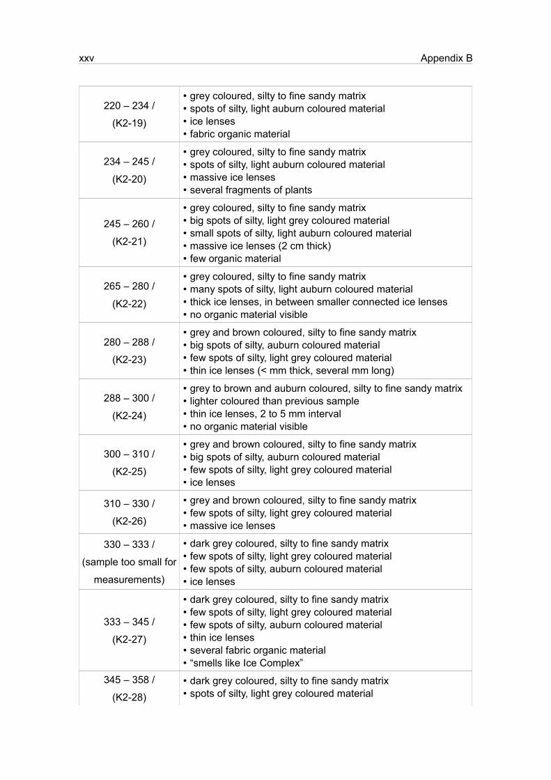
xxv Appendix B

220 – 234 /

(K2-19)

• grey coloured, silty to fine sandy matrix• spots of silty, light auburn coloured material• ice lenses• fabric organic material

234 – 245 /

(K2-20)

• grey coloured, silty to fine sandy matrix• spots of silty, light auburn coloured material• massive ice lenses• several fragments of plants

245 – 260 /

(K2-21)

• grey coloured, silty to fine sandy matrix• big spots of silty, light grey coloured material• small spots of silty, light auburn coloured material• massive ice lenses (2 cm thick)• few organic material

265 – 280 /

(K2-22)

• grey coloured, silty to fine sandy matrix• many spots of silty, light auburn coloured material• thick ice lenses, in between smaller connected ice lenses• no organic material visible

280 – 288 /

(K2-23)

• grey and brown coloured, silty to fine sandy matrix• big spots of silty, auburn coloured material• few spots of silty, light grey coloured material• thin ice lenses (< mm thick, several mm long)

288 – 300 /

(K2-24)

• grey to brown and auburn coloured, silty to fine sandy matrix• lighter coloured than previous sample• thin ice lenses, 2 to 5 mm interval• no organic material visible

300 – 310 /

(K2-25)

• grey and brown coloured, silty to fine sandy matrix• big spots of silty, auburn coloured material• few spots of silty, light grey coloured material• ice lenses

310 – 330 /

(K2-26)

• grey and brown coloured, silty to fine sandy matrix• few spots of silty, light grey coloured material• massive ice lenses

330 – 333 /

(sample too small for

measurements)

• dark grey coloured, silty to fine sandy matrix• few spots of silty, light grey coloured material• few spots of silty, auburn coloured material• ice lenses

333 – 345 /

(K2-27)

• dark grey coloured, silty to fine sandy matrix• few spots of silty, light grey coloured material• few spots of silty, auburn coloured material• thin ice lenses• several fabric organic material• “smells like Ice Complex”

345 – 358 /

(K2-28)• dark grey coloured, silty to fine sandy matrix• spots of silty, light grey coloured material

Appendix B xxvi

• few spots of silty, auburn coloured material• less ice content (few, thin lenses)

358 – 366 /

(K2-29)

• dark grey and brown coloured, silty to fine sandy matrix• few spots of silty, auburn coloured material• several fragments of plants

366 – 380 /

(K2-30)

• dark grey and brown coloured, silty to fine sandy matrix• few spots of silty, auburn coloured material• ice lenses• several fragments of plants

Eidesstattliche Erklärung

Hiermit erkläre ich an Eides Statt, dass ich die vorliegende Diplomarbeit selbst angefertigt habe

und keine anderen als die angegebenen Quellen verwendet wurden. Die aus fremden Quellen

direkt oder indirekt übernommenen Gedanken sind als solche kenntlich gemacht.

Die Arbeit wurde bisher keiner Prüfungsbehörde vorgelegt und auch noch nicht veröffentlicht.

Ort, Datum Unterschrift