measuring and analysing agricultural productivity in …pdf.usaid.gov/pdf_docs/pnads080.pdf ·...

1

Measuring and Analysing AgriculturalProductivity in Kenya: a Review of

Approaches

Walter OdhiamboHezron O. Nyangito

Productive Sector DivisionKenya Institute for Public PolicyResearch and Analysis

KIPPRA Discussion Paper No. 26January 2003

2

Measuring and analysing agricultural productivity in Kenya: a review of approaches

KIPPRA IN BRIEF

The Kenya Institute for Public Policy Research and Analysis (KIPPRA)is an autonomous institute whose primary mission is to conduct publicpolicy research, leading to policy advice. KIPPRA’s mission is to produceconsistently high-quality analysis of key issues of public policy and tocontribute to the achievement of national long-term developmentobjectives by positively influencing the decision-making process. Thesegoals are met through effective dissemination of recommendationsresulting from analysis and by training policy analysts in the publicsector. KIPPRA therefore produces a body of well-researched anddocumented information on public policy, and in the process assists informulating long-term strategic perspectives. KIPPRA serves as acentralized source from which the government and the private sectormay obtain information and advice on public policy issues.

Published 2003© Kenya Institute for Public Policy Research and AnalysisBishops Garden Towers, Bishops RoadPO Box 56445, Nairobi, Kenyatel: +254 2 2719933/4; fax: +254 2 2719951email: [email protected]: http://www.kippra.orgISBN 9966 949 46 1

The Discussion Paper Series disseminates results and reflections fromongoing research activities of the institute’s programmes. The papersare internally refereed and are disseminated to inform and invoke debateon policy issues. Opinions expressed in the papers are entirely those ofthe author or authors and do not necessarily reflect the views of theInstitute.

KIPPRA acknowledges generous support by the European Union (EU),the African Capacity Building Foundation (ACBF), the United StatesAgency for International Development (USAID), the Department forInternational Development of the United Kingdom (DfID) and theGovernment of Kenya (GoK).

3

ABSTRACT

Concern is rising about the performance of the agricultural sector in Kenya

given that it is the backbone of the country’s economy. The issue of particular

concern is the declining productivity that has been associated with increasing

poverty, food shortages and poor rural livelihoods. Although there have been

attempts to analyse agricultural productivity in Kenya, a cursory examination

of the existing studies reveals quite varied approaches to the measurement and

analysis of productivity. Variability in the analytical methods and data

employed make it difficult for policy makers, the Government, NGOs and even

donors to interpret, compare and evaluate the results of such studies. The

objective of this paper is to review studies that have attempted to empirically

measure and analyse agricultural productivity in Kenya. The focus of the survey

is on the approaches that have been used and their relevance in policy

formulation. The major conclusion of the study is that although there have

been attempts to analyse agricultural productivity in Kenya, the approaches,

the data used, as well as the scope have largely been inadequate. This has

hampered policy formulation for the development of agricultural productivity.

The paper therefore identifies research gaps and proposes new directions in the

measurement and analysis of agricultural productivity in Kenya.

4


ABBREVIATIONS

CBS Central Bureau of Statistics (Kenya)

C-D Cobb-Douglas

CES Constant Elasticity Substitution

DEA Data Enveloping Analysis

GLS Generalized Least Squares

MLE Maximum likelihood method

OLS Ordinary Least Squares

PFT Partial factor productivity

TFP Total factor productivity

3SLS Three-Stage Least Squares

5

TABLE OF CONTENTS

1. Introduction ............................................................................... 1

2. Theoretical approaches of measuring agricultural

productivity ................................................................................ 3

2.1. Technical progress ........................................................... 4

2.2 Productivity growth ....................................................... 5

2.3 Efficiency .......................................................................... 7

2.4 Total factor productivity ................................................. 8

2.5 Measuring total factor productivity ............................. 9

2.5.1 Approaches that ignore inefficiency ................... 9

2.5.2 Approaches that incorporate inefficiency ........ 13

3. Review of agricultural productivity studies in Kenya..... 24

3.1 Empirical studies on productivity .............................. 24

3.1.1 Macro studies ....................................................... 24

3.1.2 Messo studies ....................................................... 27

3.1.3 Micro studies ........................................................ 30

3.2 Empirical determinants of productivity .................... 34

3.2.1 Resources inputs .................................................. 34

3.2.2 Fertilizer use ......................................................... 35

3.2.3 Market access and orientation ........................... 36

3.2.4 Extension services ................................................ 37

3.2.5 Farm size ............................................................... 38

3.2.6 Biophysical factors .............................................. 38

3.2.7 Land tenure .......................................................... 39

4. Evaluation of previous work and new directions in

empirical research .................................................................... 40

4.1. Average versus marginal productivity indicators .... 40

4.2 Use of alternative models ............................................. 41

4.3 Model specification ....................................................... 42

4.4 Issues of resource use efficiency .................................. 42

4.5 Environmental impact .................................................. 43

4.6 Effects of transaction costs ........................................... 44

4.7 Data types and sources ................................................. 45

5. Conclusions and implications for further research ......... 47

References ................................................................................... 49

6


7

1. Introduction

The improvement of agricultural productivity has attracted the attention

of policy makers, researchers and development practitioners in Kenya

for two main reasons. First, Kenya relies heavily on agriculture for

economic growth, export earnings, and employment generation. The

agricultural sector employs 70% of the Kenyan labour force, generates

60% of the foreign exchange, provides 75% of raw materials for industry,

and provides about 45% of total Government revenue. Besides, the sector

is the growth engine for the non-agricultural sector with a multiplier

effect of about 1.64. Second, indications in Kenya, and in many other

sub-Saharan African countries, are that agriculture is becoming

progressively less productive. A declining trend in both labour and land

productivity constitutes a major challenge and portends lower living

standards in the farm sector and the rest of the economy.

Literature in Kenya and in other developing countries is abound with

discussions of factors considered to be important in determining

agricultural productivity. These include quantifiable factors such as

technical change, relative factor product prices, input use, education,

agricultural research and extension, market access and availability of

credit. Other factors include weather, farm production policies, land

ownership patterns, inadequate involvement of beneficiaries in

decision-making, insecurity and the legal and regulatory environment.

Many development programs and projects in Kenya have attempted to

remove constraints associated with these factors by introducing facilities

to provide credit, information, farm inputs, infrastructure, education,

marketing networks, etc. The removal of these constraints, it is believed,

can result in increased productivity at farm level and also an increase

in farm incomes. This is important for alleviating poverty, increasing

household food security, and stimulating growth in non-farm activities

in Kenya. Indeed, declining agricultural productivity has been identified

as a major cause of poverty in Kenya. According to the Kenya Poverty

8


Reduction Strategy Paper (PRSP), declining agricultural productivity

has led to food shortages, underemployment, low incomes from cash

crops and poor nutritional status which further reduces labour

productivity (Republic of Kenya, 2001).

Assessing the overall impact of interventions in agriculture and

reversing the declining trend in productivity requires accurate

measurement of the effects of alternative courses of action, a task that

raises conceptual and methodological issues. A cursory examination of

the literature on productivity in the country reveals quite varied

measurement and analytical approaches. Variability in the analytical

methods and data used make it difficult for policy makers, NGOs, and

even donors to interpret, compare and evaluate the results of

productivity studies. This has led to differing conclusions, which have

sometimes conflicted. Another issue of concern is that writings on

various aspects of agricultural productivity are either too old and need

regular updating or are scattered through a wide variety of sources in

the country. As the Government implements new agricultural policies

and programs aimed at increasing overall productivity, it is important

that it accesses accurate agricultural data and analyses. Poor agricultural

data and analyses can lead to misallocation of scarce resources and

formulation of policies that fail to resolve critical challenges in the sector.

The purpose of this paper is to survey various studies that have

attempted to measure and analyse agricultural productivity in Kenya.

The focus of the survey is on the strengths and weaknesses of the

different approaches that have been used to measure and analyse

agricultural productivity. Because of the diversity of such published

work, an attempt is made to simply review representative works rather

than present an exhaustive discussion of all that has been done. The

next section introduces a number of key concepts and the conceptual

framework for measuring and analysing agricultural productivity.

Section three presents a review of empirical approaches and results of

9

studies on agricultural productivity in Kenya. Section four takes a critical

look at the approaches, the data used, and the conclusions of the

empirical studies of agricultural productivity in Kenya. The conclusions

and implications for further research and analysis are presented in the

last section.

2. Theoretical Approaches of Measuring

Agricultural Productivity

The aim of this section is to review the theoretical approaches for

measuring agricultural productivity in the wider literature. The section

first gives the definition of key concepts, namely technical progress,

productivity growth and efficiency. This is necessary in providing a

common understanding of the usage of these terms in analysis of

agricultural productivity. The section then looks at the theoretical

approaches and methodologies used in the literature to measure

agricultural productivity.

Before defining key concepts in productivity analysis, it is important to

note at the outset that works on agricultural productivity can be broadly

classified into two groups: theoretical and empirical. Theoretical studies

define productivity and its determinants more rigorously and set precise

relationships for estimation. They also suggest hypotheses that can be

tested empirically. Empirical studies on the other hand examine trends

over time and quantify the contributions of specific inputs, policies,

technologies and other productivity-enhancing factors. In the realm of

empirical studies, Kelly et al (1995), in a similar survey to this one,

identify three categories of productivity work in agriculture. These are

“macro”, “messo” and “micro” studies. Macro studies use time series

data reported at the national level, while messo studies use national

data disaggregated into farm types (large or small), agro-ecological

zones, or administrative regions. Micro studies use cross-sectional

Introduction

10


data, which permit comparison across different sub-groups at a

particular point in time. This review is organized around this broad

categorization. While this section examines the theoretical

underpinnings of productivity, the next section reviews empirical micro,

messo and macro studies on agricultural productivity in Kenya.

2.1 Technical Progress

Methods of production change over time and it is important to be able

capture the effects of such changes on output. Capturing such effects

can ideally be done within the production function framework. Starting

of with a simple production relationship in which output depends on

capital input K, and labour L, the production function can be expressed

as:

Q=f(K, L)......................................................................................(1)

where Q (the output) depends on how much of K and L is used. If the

levels of K and L are increased/reduced, then it is expected that Q will

also correspondingly increase/decrease. However, Q can also increase

by using the same level of K and L. This is possible if a superior

technology is used in the production process. However, output growth

can also be attributed to other factors other than growth in the

conventionally defined inputs. When this is the case, then technical

progress has taken place. In terms of the production relations, such a

change represents a shift in the production frontier and can be defined

as:

Q=A(t)f(K, L).................................................................................(2)

where A(t) represents all the influences that go into determining Q

besides K and L. Changes in A over time represent technical progress.

It is important to note that technical change may influence output in

two distinct ways. First, technical change may influence output by

11

affecting not a single input but all the inputs. This would be a case of

neutral technical progress or disembodied technical progress. Equation

(1) above is a case of neutral technical progress. The second case is where

technical change affects output by augmenting either capital (capital-

augmenting technical progress) or labour (labour-augmenting technical

progress). These two cases are commonly referred to as disembodied

technical progress and can be represented as:

Q =f[A(t)K, L]...............................................................................(3)

and

Q= f[K, A(t)L]....................................................................................(4)

Equation (3) represents the capital-augmenting technical progress while

equation (4) is a case of labour-augmenting technical progress. In all

the three cases represented by equations (2)-(4), the empirical question

is how to measure A(t).

2.2 Productivity Growth

The concept of technical progress is closely related to productivity

growth. In fact, productivity growth has been shown to be a major source

of growth of aggregate output (Solow, 1957) and of agricultural output

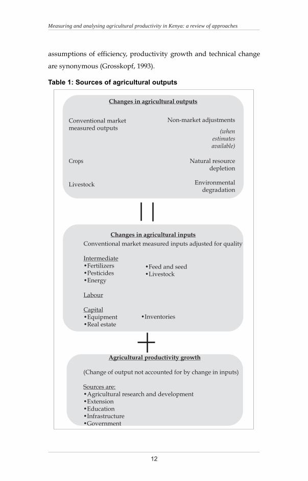
(Hayami and Ruttan, 1985). Hayami and Ruttan (1985) have shown that

agricultural output can grow in two main ways: an increase in use of

resources of land, labour, capital and intermediate inputs or through

advances in techniques of production through which greater output is

achieved through a constant or declining resource base. This relationship

is shown in Table 1. The latter, also referred to as productivity, occurs

without a corresponding change in output, occasioning a rise in the

ratio of total outputs to inputs. Seen in this way, productivity can be

defined simply as a measure of the increase in output that is not

accounted for by the growth of production inputs. Under certain

Theoretical approaches of measuring agricultural productivity

12


assumptions of efficiency, productivity growth and technical change

are synonymous (Grosskopf, 1993).

Table 1: Sources of agricultural outputs

Changes in agricultural inputs

Conventional marketmeasured outputs

Non-market adjustments

(whenestimatesavailable)

Crops Natural resourcedepletion

Livestock Environmentaldegradation

Conventional market measured inputs adjusted for quality

Intermediate•Fertilizers•Pesticides•Energy

Labour

Capital•Equipment•Real estate

Changes in agricultural outputs

•Feed and seed •Livestock

•Inventories

Agricultural productivity growth

(Change of output not accounted for by change in inputs)

Sources are:•Agricultural research and development•Extension•Education•Infrastructure•Government

13

Conventionally, productivity is measured by an index of output divided

by inputs. Two measures of productivity are frequently used: the partial

factor productivity (PFP) and total factor productivity (TFP). PFP is

simply the ratio of output and any one of the inputs, typically labour or

land. In notation form this can be expressed as:

PFP =Y/Xi.......................................................................(5)

where Y is output and X is input i. Although commonly used, the partial

productivity measure has one important weakness in that it does not

control for the level of other inputs employed. TFP on the other hand

measures output per unit of total factor inputs. Therefore, total factor

productivity is a generalization of single factor productivity measures

such as land productivity or labour productivity.

2.3 Efficiency

The concept of technical efficiency entails a comparison between

observed and optimal values of output and inputs of a production unit

(Sadoulet and Janvry, 1995). This comparison takes the form of the ratio

of observed to maximum potential output obtainable from the given

input, or the ratio of the minimum potential to observed input required

to produce the given output, or some combination of the two. These

two give rise to the concepts of technical and allocative efficiency. A

productive entity is technically inefficient when, given its use of inputs,

it is not producing the maximum output possible (output distance), or

given its output, it is using more inputs than is necessary. Similarly, a

production unit is allocatively inefficient when it is not using the

combination of inputs that would minimise the cost of producing a given

level of output (Sadoulet and Janvry, 1995).

Efficiency and productivity are closely related. Changes in productivity

are due to differences in production technology, differences in the

efficiency of the production process, and differences in the environment


14


in which production takes place (Grosskopf, 1993). Productive efficiency

is therefore an important determinant of productivity and should be

incorporated in productivity analyses. The empirical challenge is to

measure productive efficiency and to apportion its share in the

productivity variations.

2.4 Total Factor Productivity

As already indicated, most analyses of agricultural productivity have

utilised the TFP concept. Because of its superiority over other measures

of productivity, TFP is examined in some detail in this sub-section.

Grosskopf (1993) outlines the basic procedure for deriving the TFP index.

Considering two time periods t and t+1, corresponding outputs and

inputs denoted by yt and yt+1 and xt and xt+1, the production

transformation model St, for period t can be expressed as:

St ={(xt, yt): xt can produce yt}......................................(6)

Similarly for St+1

St+1 = {(xt+1, yt+1): xt+1 can produce yt+1 }.......................(7)

The set S describes all the feasible input-output pairs at a given point in

time. In a similar manner, technology can also be described with a

production function in period t as

yt = max {y’t : (xt, y’t) εSt}………………….…………….(8)

and in period t+1

yt+1 = max {y’t+1 : (xt+1, y’t+1) ε St+1}…………….………(9)

Assuming neutral disembodied technology in the Hicksian sense (that

is technology independent of input) the production functions in the

two periods can be denoted by:

yt = A(t)f(xt )

15

yt+1 = A(t+1)f (xt+1 ).....................................................................(10)

where A is a technology shift parameter.

Based on equation (10), total factor productivity (TFP) can be defined

for the two periods as:

TFP(t) = yt/f(xt ) = A(t)

TFP(t+1) = yt+1/ f(xt+1 ) = A(t+1)..................................................(11)

The total factor productivity growth can then be defined as the change

in total factor productivity between period t and t+1, that is:

TFP(t+1)/TFP(t) = A(t+1)/A(t)...................................................(12)

It needs to be noted here that technical change and productivity growth

are synonymous in the special case when production is technically

efficient (Grosskopf, 1993).

2.5 Measuring Total Factor Productivity

As stated earlier, the empirical challenge is to estimate A(t) in equation

(12). In the literature there are two different approaches of doing this.

The major difference in the approaches is the assumption made about

technical efficiency. Traditional approaches of measuring productivity

assume that output is technically efficient and that production is taking

place at the frontier of the production. Recent approaches allow for

inefficiency. The following subsection reviews these two broad

approaches to the estimation of TFP.

2.5.1 Approaches that ignore inefficiency

Non-parametric approaches

Until very recently, models of productivity have ignored efficiency as a

determinant of productivity. Solow (1957) sought to attribute output


16


growth to input growth and technical change by distinguishing

movements along a production frontier from shifts in the frontier. From

a production function of the form shown in equation (8), Grosskopf

(1993) postulates the decomposed Solow model to be of the form:

−= ∑

− n

nN

n

nx

xS

y

y

A

A

1

.................................................(13)

where the dots indicate time derivatives and sn is the elasticity of output

with respect to inputs. Equation (13) gives the accounting definition of

productivity as the residual growth in output not accounted for by

growth in input. This definition is associated to Solow (1957), Denison

(1972), Kendrick (1961) and Jorgenson and Griliches (1967).

To compute equation (13), Solow made the assumption that the time

derivatives could be approximated by discrete changes. This assumption

results in a non-parametric growth index equivalent to the Divisia Index

of productivity growth. Grosskopf (1993) shows that if the continuous

growth rates in equation (13) above are replaced by the discrete

difference in the logarithms (i.e. y’/y = ln yt+1 – ln yt) and the input

shares as arithmetic means, the index becomes equivalent to the

Tornqvist (1936) index (π) of total factor productivity growth, which

takes the form (the variables are as defined before):

...........(14)

The Tornqvist index has been widely used to calculate the annual index

of TFP. The index can either be a price or quantity index. It has one

advantage in that it is simple and easy to compute. This is because there

are no parameters to be estimated in the model. The only weakness

with the index is that it does not account for measurement or sampling

errors. As such, it leaves out departures from efficient production due

to measurement errors (noise) or technical inefficiency.

( ) ( )[ ]( )tn1t

nnn

N

1n

t1t

1 lnxlnxtS1tS2

1lnylnyLnT −++∑−−= +

−

+

. . .

17

Econometric approaches

The econometric approach is often the alternative to the non-parametric

index approach. The approach involves parametizing the production

function and estimating its parameters. This would take the form of

yt = f(xt , t) + ε……………………………………….....………(15)

for t=1, 2….T and where ε is intended to capture the effect of stochastic

noise. The estimated parameters from the model can then be used to

solve for technical change in the model. In the absence of technical

inefficiency, the technical change will be the TFP and will be reflected

in the vertical shifts in the production function; that is by increases in

output that are not accounted for in increases in use of inputs.

Mathematically, TFP can be computed as the difference between output

and weighted average of the inputs. The weights are estimated

econometrically from the production coefficients in the agricultural

production functions. Using a Cobb-Douglas production function with

capital K and labour L, Block (1994) estimated TFP as:

TFP = log Y-β1logK– β

2logL………………………………….(16)

where Y is output and β1

and β2 are parameters. In computing

agricultural productivity, Equation (16) can be expanded to include other

factor inputs that determine productivity, such as land and fertilizers.

The duality relationship between the production function and the cost

function has also been used to estimate TFP. The duality hypothesis

stipulates that for every production function, there is a dual cost function

relating factor prices to the cost of output. The dual cost function

contains all the information that the production function contains

(Varian, 1992). Biswanger (1974) has shown the cost function to be more

desirable for econometric analysis than the production function for a

variety of reasons. First, that by using the cost function approach, the

problem of endogeneity in factor levels is eliminated since factor prices


18


and output levels are exogenous. Second, that the cost function approach

reduces the problem of multi-collinearity since less multi-collinearity

exists among factor prices than factor quantities. Third, the approach

yields direct estimates of the various elasticities of substitution. It is

worth noting at this point that this approach involves the estimation of

the cost function along with the input demand functions derived from

the Hotellings lemma. The duality approach does not however explicitly

take efficiency issues into consideration. In other words it is not possible

to isolate the efficiency effects from other effects using this approach.

The dual approach in the analysis of productivity and efficiency can be

demonstrated by considering both the Cobb-Douglas (C-D) and the

constant elasticity of substitution (CES) production functions which are

the most widely used forms. Equations (17) and (18) depict the C-D

and CES production functions.

Y = γx1αx

2β………………………………………………….…..(17)

where β=1-α, and

Y=λ(δx1

-ρ+(1-δ)x2

-ρ)-v/ρ………………………………….………(18)

where λ, ρ, δ and v are efficiency, distribution and substitution

parameters. Given that C=r1x

1=r

2x

2 is the corresponding dual cost

function for the C-D and CES production functions are:

=

−−

v

r

rv

r

r

v

rrY

C

αβ

β

α

α

βλ

)(2)(1)(

1

2

2

1

1………………….(19)

where v=α+β and

…………................……..(20)C = Y [δ r1 (1−δ)r ] γ

-1v σ 1-σ 1-σ 1-σ

1

19

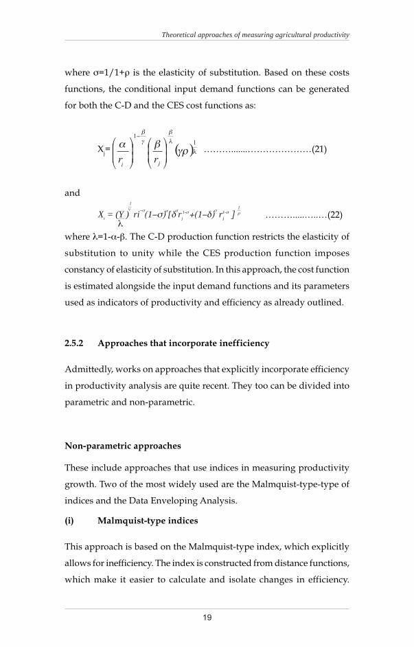
where σ=1/1+ρ is the elasticity of substitution. Based on these costs

functions, the conditional input demand functions can be generated

for both the C-D and the CES cost functions as:

Xj= ( )λ

λ

β

γ

β

γρβα 1

1

−

jirr

……….......…………………(21)

and

……….....…..…(22)

where λ=1-α-β. The C-D production function restricts the elasticity of

substitution to unity while the CES production function imposes

constancy of elasticity of substitution. In this approach, the cost function

is estimated alongside the input demand functions and its parameters

used as indicators of productivity and efficiency as already outlined.

2.5.2 Approaches that incorporate inefficiency

Admittedly, works on approaches that explicitly incorporate efficiency

in productivity analysis are quite recent. They too can be divided into

parametric and non-parametric.

Non-parametric approaches

These include approaches that use indices in measuring productivity

growth. Two of the most widely used are the Malmquist-type-type of

indices and the Data Enveloping Analysis.

(i) Malmquist-type indices

This approach is based on the Malmquist-type index, which explicitly

allows for inefficiency. The index is constructed from distance functions,

which make it easier to calculate and isolate changes in efficiency.


Xi = (Y ) ri (1−σ) [δ r

j +(1−δ) r

i ]

1v −σ

λ

σ σ 1-σ σ 1-σ ρ1

20


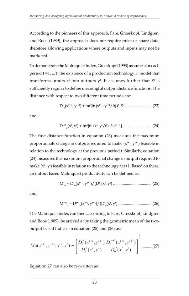
According to the pioneers of this approach, Fare, Grosskopf, Lindgren,

and Roos (1989), the approach does not require price or share data,

therefore allowing applications where outputs and inputs may not be

marketed.

To demonstrate the Malmquist Index, Grosskopf (1993) assumes for each

period t =1, ...T, the existence of a production technology St model that

transforms inputs xt into outputs yt. It assumes further that St is

sufficiently regular to define meaningful output distance functions. The

distance with respect to two different time periods are:

Dto(xt+1 , yt+1) + inf{θ: (xt+1, yt+1/θ) ε St }………….…….(23)

and

Dt+1o(xt, yt) + inf{θ: (xt, yt/θ) ε St+1 }………………….(24)

The first distance function in equation (23) measures the maximum

proportionate change in outputs required to make (xt+1, yt+1) feasible in

relation to the technology at the previous period t. Similarly, equation

(24) measures the maximum proportional change in output required to

make (xt , yt) feasible in relation to the technology at t+1. Based on these,

an output based Malmquist productivity can be defined as:

Mto = Dt

o(xt+1, yt+1)/(Dt

o(xt, yt) .....................................(25)

and

Mt+1o = Dt+1

o(xt+1, yt+1)/(Dt

o(xt, yt).................................(26)

The Malmquist index can then, according to Fare, Grosskopf, Lindgren

and Roos (1989), be arrived at by taking the geometric mean of the two-

output based indices in equation (25) and (26) as:

2

1

),(

),(

),(

),(),,,(

0

111

0

0

11

01110

=

+++++++

ttt

ttt

ttt

ttt

tttt

yxD

yxD

yxD

yxDyxyxM ..........(27)

Equation 27 can also be re-written as:

21

( )( )

( )( )

( )( )

2

1

1111

11

9

111

0110

,

,

,

,

,

,),,,(

= ++++

+++++++

ttt

o

ttt

o

ttt

o

tt

o

ttt

ttt

tttt

yxD

yxD

yxD

yxD

yxD

yxDyxyxM

........(28)

Based on equation (23), the efficiency change (EC) and the technical

change (TC) can be expressed as:

( )( )ttt

ttt

yxD

yxDEC

,

,

0

111

0

+++

= ...........................................................(29)

and

.............................(30)

(ii) Data Enveloping Analysis

Recent mathematical programming approaches in the measurement of

productive efficiency have mainly taken the form of data enveloping

analysis (DEA). This approach is commonly used to evaluate the

efficiency of a number of producers. Unlike other statistical procedures

that evaluate each producer relative to the average producer, DEA

compares each producer with only the “best” producers. The

fundamental assumption here is that if a given producer A is capable of

producing output Y(A) with X(A) inputs, then other producers should

be able to do the same if they were to operate efficiently. Similarly, if a

producer B is capable of producing Y(B) units of output with X(B) inputs,

then other producers should also be capable of the same production

schedule. Producer A, B and others can then be combined to form a

composite producer with composite inputs and composite outputs.

Since this composite producer does not necessarily exist, it is sometimes

called the virtual producer.

The gist of the analysis in DEA is finding the best virtual producer for

each real producer. If the virtual producer is better than the original

producer by either making more output with the same inputs or making

( )( )

( )( )

2/1

1

0

0

111

111

0

,

,

,

,

= ++++

+++

ttt

ttt

ttt

ttt

yxD

yxD

yxD

yxDTC


22


the same output with less input, then the original producer is inefficient

(Lovell, 1993). The procedure of finding the best virtual producer can

be formulated as a linear program. Analysing the efficiency of n

producers is then a set of n linear programming problems. The

programming approach, like the econometric one, can be categorized

according to the type of data used (cross-section or panel) and according

to the type variables (quantities only or quantities and prices). While it

is possible to measure technical efficiency with quantities only, it is

necessary to have both prices and quantities to measure economic

efficiency. Lovell (1993) provides a very good review of the mathematical

programming approaches to the measurement of efficiency.

DEA has a number of advantages over the other measures of efficiency.

(i) DEA can handle multiple input and multiple output models.

(ii) Unlike the econometric approaches, DEA does not require an

assumption of a functional form relating inputs to outputs.

(iii) DEA can handle inputs and output in different units. It can

handle both quantities and prices measured in different units.

DEA is also associated with a number of weaknesses:

(i) Since DEA is an extreme point technique, its results are very

sensitive to noise (even symmetrical noise with zero mean).

(ii) Since DEA is a non-parametric technique, statistical hypotheses

tests are difficult.

(iii) Where a large number of producers are involved, DEA can be

computationally intensive.

It is important to note that the application of DEA in agriculture has for

reasons related to data been very limited. DEA has been applied in

situations such as healthcare (hospitals, doctors), education, banks,

manufacturing, management evaluation, fast foods restaurants and

retail stores.

23

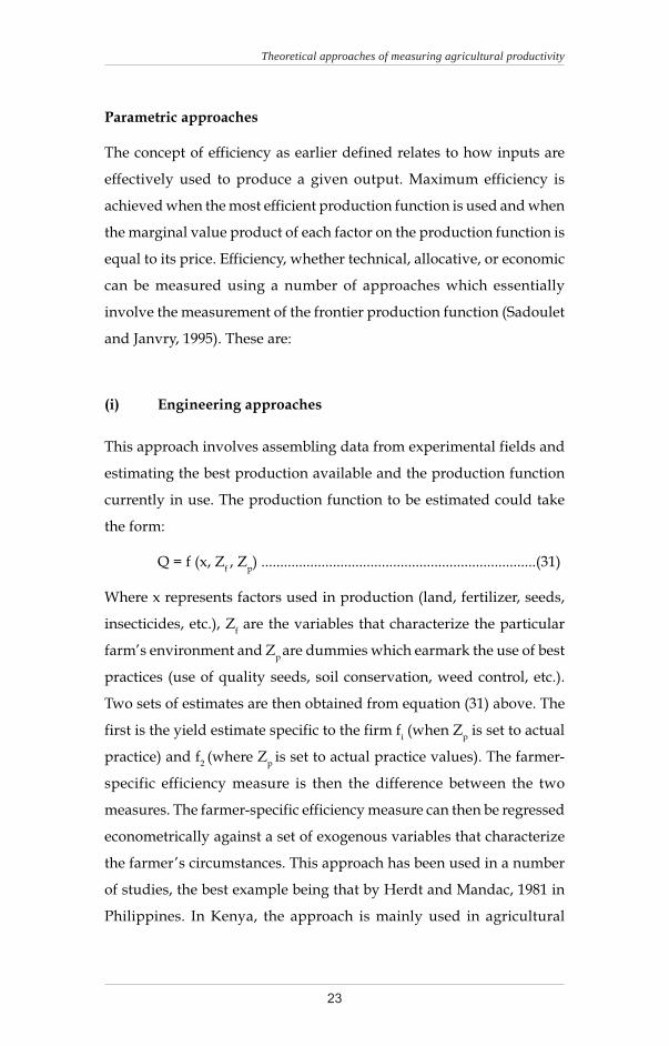
Parametric approaches

The concept of efficiency as earlier defined relates to how inputs are

effectively used to produce a given output. Maximum efficiency is

achieved when the most efficient production function is used and when

the marginal value product of each factor on the production function is

equal to its price. Efficiency, whether technical, allocative, or economic

can be measured using a number of approaches which essentially

involve the measurement of the frontier production function (Sadoulet

and Janvry, 1995). These are:

(i) Engineering approaches

This approach involves assembling data from experimental fields and

estimating the best production available and the production function

currently in use. The production function to be estimated could take

the form:

Q = f (x, Zf , Z

p) .........................................................................(31)

Where x represents factors used in production (land, fertilizer, seeds,

insecticides, etc.), Zf are the variables that characterize the particular

farm’s environment and Zp are dummies which earmark the use of best

practices (use of quality seeds, soil conservation, weed control, etc.).

Two sets of estimates are then obtained from equation (31) above. The

first is the yield estimate specific to the firm fi (when Z

p is set to actual

practice) and f2 (where Z

p is set to actual practice values). The farmer-

specific efficiency measure is then the difference between the two

measures. The farmer-specific efficiency measure can then be regressed

econometrically against a set of exogenous variables that characterize

the farmer’s circumstances. This approach has been used in a number

of studies, the best example being that by Herdt and Mandac, 1981 in

Philippines. In Kenya, the approach is mainly used in agricultural


24


research stations and increasingly on on-farm research. Its results usually

form the basis of input use recommendations by agricultural research

institutions.

This approach has a number of advantages that make it appealing in

the assessment of efficiency in agriculture (Sadoulet and Janvry, 1995):

(i) The approach is simple and straightforward. Its results are also

very easy to interpret.

(ii) The data required for this analysis is directly generated from

the experiments, and are likely to be more accurate than data

collected by other means.

(iii) The approach generates a good indicator of efficiency that

incorporates and reflects on technical changes associated with

different methods of production, technologies, etc.

(ii) Use of average production functions

This is a particularly useful method of measuring differences in technical

and allocative efficiencies between different categories of farms (e.g.

small and large), different regions, and over time. The approach involves

the estimation of a production function with farm, regional or time

dummies included in the function. The dummies in the functions are

meant to capture allocative and technical efficiency differentials.

Yotopoulos and Lau (1973) provide a good example of this approach

for estimating efficiency. In their analysis, the two authors specify and

estimate a Cobb-Douglas production and profit functions of the form:

Q = axαzβ……………………....……………………………….(32)

and

π = a*zβ*p1-α*wα*…………………………………………………(33)

Where x is labour used in production with corresponding wage w, z is

a fixed factor, q is output with corresponding price q, and π is profit.

25

The other variables, namely α and β and a are parameters1. Based on

these, Yotopoulos and Lau (1973) formulated and estimated the model

below using time series data:

Ln π =ln a* + δlD

l +£*´

tD

t+α* ln w + (1-α*)ln p + £β*

mln z

m

-wx/π =λlD

l + λ

sD

s……………....................…………………(34)

where Dl, D

s, and D

t are dummies for large farms, small farms and time.

The relevant estimation procedure here is the Zellner seemingly

unrelated regression method. This approach requires data on the inputs

used, prices, and profits disaggregated by type of farm or region. The

obvious advantage of this approach is that it accounts for differences in

efficiency between different categories of producers or regions. As

already indicated, there are marked differences in terms of resource

use and style of production between large and smallscale. There are at

the same time significant regional differences in agricultural potentiality

and efficiency. The main weakness of the approach has to do with the

use of the production functions in estimation of efficiency. The first issue

is which between the Cobb-Douglas and the CES (or indeed any other

form) is the most appropriate functional form of the production function.

The second issue has to do with the assumptions made in each case.

The Cobb-Douglas production function restricts the elasticity of

substitution to unity while the CES production function imposes

constancy of elasticity of substitution. These are not particularly realistic

assumptions in the context of agricultural production.

(iii) Stochastic frontier analysis

The use of econometric techniques in estimation of efficiency has

increased considerably in recent times. This has mainly taken the form

of estimating a frontier production function. Econometric approaches


1 It can be shown that a*=a1/1-α α α/1-α, β* =β/1-β and α*=-α/1-α

26


developed by Aigner, Lovell and Schmidt (1977) are among the first to

use non-stochastic frontier methods of estimation. Since then, there have

been several attempts to use the technique. These attempts vary

according to the type of data used (cross-section or panel), the type of

variables (quantities only, or quantities and prices) and the number of

equations in the model.

(a) Cross-sectional designs

These are by far the most widely used techniques in the estimation of

productive efficiency. The process involves the specification and

estimation of a production function of the form:

Yi = f(x

i, β) exp {v

i + u

i)………………………........…………..(35)

where β is a vector of technology parameter, x are the inputs used and

i=1….I indexes producers. The model specifies two random disturbance

terms vi and u

i.. The random disturbance term v

i is intended to capture

the effects of the stochastic noise. It is assumed to be independently

distributed with a mean equal to zero and standard deviation equal to

σ2v. The disturbance term u

i captures technical inefficiency and is

assumed to be independent of vi. Lovell (1993) shows that the technical

efficiency (TE) can be expressed as a reciprocal of the Dubreau-Farrel

output oriented technical efficiency. This can be written as:

TEi = ............................................(36)

Estimation of technical efficiency was first accomplished by Aigner,

Lovell and Schmidt (1977), Battese and Corra (1977) and Meeusen and

Van den Broeck (1977). These studies provide estimates of the average

technical efficiency over all the observations. The data used was cross-

sectional in nature. To estimate the equations, a number of assumptions

are necessary. First, it can be assumed that vi=0 and then estimate a

deterministic production frontier. The maximum likelihood method

(MLE) can then be used as an estimation procedure in this case. The

}{[ ] { }i

ii

i uv)expxf

yexp

;(=

β

27

second assumption will be to assume that vi≠0 and estimate a stochastic

production frontier. MLE can also be used in this particular case.

It should be noted that the models above are single–equation models

and would require the use of single equation techniques. However, it is

also possible to specify and estimate multiple equation models. This is

usually more appropriate in order to go around the weaknesses of single

equations. By assuming profit maximization behaviour, this approach

can be used to yield consistent and efficient estimates of economic

efficiency. The approach essentially involves the estimation of a

production frontier and the first order conditions for profit

maximization. Starting from a typical production relationship of the

form (Sadoulet and Janvry, 1995):

q* = f (x) .....................................................................................(37)

where q* is the maximum output a firm/producer could reach by using

the inputs in a technically efficient manner. If the producer is not

technically efficient, the predicted level of output with the observed

level of inputs will be:

q =f(x) eu, u ≤ 0………………………………………………….(38)

where eu is the producer-specific technical efficiency parameter. If the

firm is maximally efficient, u=0. If the producer is technically inefficient,

u<0 and q<q*. In the collection of data, measurement errors are in most

cases unavoidable and the observed level of q will therefore depend

both on the technical error term u, and v which captures noise.

q =f(x)eu+v, E(v)=0 .....................................................................(39)

If we then assume that producers are profit maximizers, then both the

output and input levels are endogenous. This has the implication that

both of these functions must be estimated simultaneously. According

to Sadoulet and Janvry (1995), the system of equation to be estimated

is:


28


Ln q = ∑∑∑= ==

++++m

i

m

j

jij

m

ii vuxx1 111

ln2

1ln γβα

∑=

=++=m

j

jjijii miwxC1

.....,1,lnγβ...............................(40)

where Ci is the share of the factor I in total revenue, calculated as p

ix

i/

pq. This model can be estimated using the maximum likelihood

approach.

Cross-sectional analyses of efficiency by their very nature provide a

snapshot of the situation at only one particular point in time. The use

of such a technique is associated with a number of advantages:

(i) It is possible to include many variables in the analysis as the

data is obtained from a large number of subjects (in this case

farmers).

(ii) The technique also allows for collection of data on attitudes

and behaviours that may have a bearing on efficiency.

(iii) The technique also allows for the analysis of dispersed subjects,

in this case farmers, in different regions or of different sizes.

Cross-sectional techniques of efficiency analysis however have a number

of disadvantages:

(i) Cross-sectional data are typically more difficult to collect and

are associated with increased chances of error.

(ii) The techniques are typically more expensive as they cover more

subjects and areas.

(iii) Cross-sectional techniques cannot measure changes,

particularly technological changes, that are a key determinants

of efficiency.

(iv) The approach is static and time bound.

29

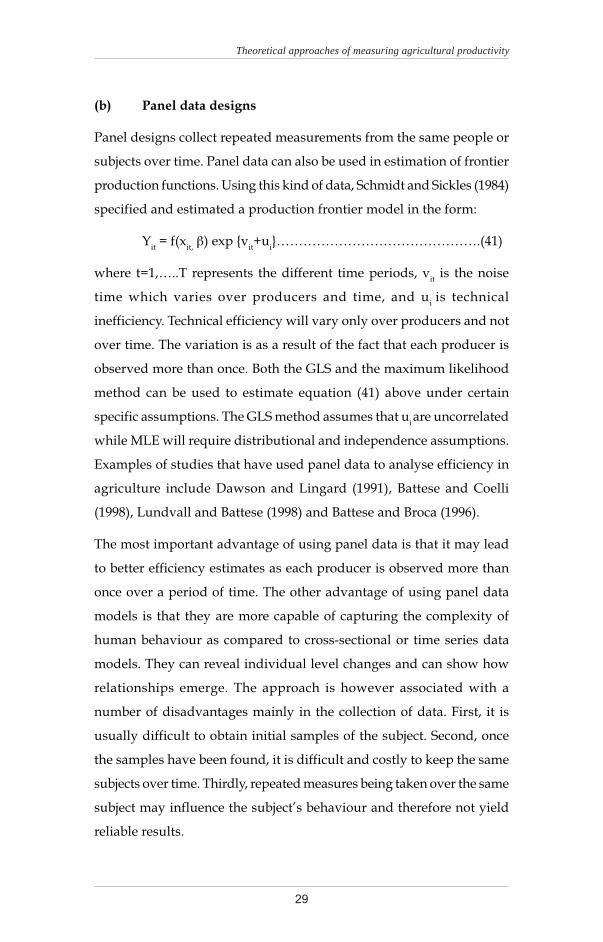
(b) Panel data designs

Panel designs collect repeated measurements from the same people or

subjects over time. Panel data can also be used in estimation of frontier

production functions. Using this kind of data, Schmidt and Sickles (1984)

specified and estimated a production frontier model in the form:

Yit = f(x

it, β) exp {v

it+u

i}……………………………………….(41)

where t=1,…..T represents the different time periods, vit is the noise

time which varies over producers and time, and ui is technical

inefficiency. Technical efficiency will vary only over producers and not

over time. The variation is as a result of the fact that each producer is

observed more than once. Both the GLS and the maximum likelihood

method can be used to estimate equation (41) above under certain

specific assumptions. The GLS method assumes that ui are uncorrelated

while MLE will require distributional and independence assumptions.

Examples of studies that have used panel data to analyse efficiency in

agriculture include Dawson and Lingard (1991), Battese and Coelli

(1998), Lundvall and Battese (1998) and Battese and Broca (1996).

The most important advantage of using panel data is that it may lead

to better efficiency estimates as each producer is observed more than

once over a period of time. The other advantage of using panel data

models is that they are more capable of capturing the complexity of

human behaviour as compared to cross-sectional or time series data

models. They can reveal individual level changes and can show how

relationships emerge. The approach is however associated with a

number of disadvantages mainly in the collection of data. First, it is

usually difficult to obtain initial samples of the subject. Second, once

the samples have been found, it is difficult and costly to keep the same

subjects over time. Thirdly, repeated measures being taken over the same

subject may influence the subject’s behaviour and therefore not yield

reliable results.


30


3. Review of Agricultural Productivity

Studies in Kenya

Having reviewed empirical and theoretical approaches entrenched in

the wider literature, this section focuses on studies that have been done

in Kenya. The aim is to delineate the approaches used in the analysis,

spell out their strengths and weaknesses, and examine the nature and

quality of data sets used. Studies on agricultural productivity in Kenya

can broadly be classified into two categories: empirical and descriptive.

Empirical studies are those that in one way or the other attempt some

measurement of productivity. Descriptive studies on the other hand

identify and discuss factors associated with agricultural productivity

without necessarily providing empirical evidence. This review focuses

more on empirical studies of measuring agricultural productivity.

3.1 Empirical Studies on Productivity

Empirical studies on productivity in Kenya have generally attempted

to provide evidence on the relative importance of different productivity

determining factors and to assess trends regionally and over time. While

most of them are at the macro level, some are micro and messo. Table 2

is a summary of some of the empirical studies on productivity in Kenya.

3.1.1 Macro studies

Two studies that attempt an estimation of agricultural productivity in

Kenya at a macro level are Block (1992) and Block and Timmer (1994).

In these studies, agricultural TFP is defined as the difference between

output and a weighted average of the inputs. Given a typical Cobb-

31

Au

tho

r Sco

pe/

da

ta M

easu

re of p

rod

uctiv

ity A

na

lytica

l focu

s T

yp

e of a

na

lysis

Table 2: S

tud

ies on

agricu

ltural p

rod

uctivity in

Ken

ya

To

tal fa

ctor p

rod

uctiv

ity (T

FP

)

To

tal fa

ctor p

rod

uctiv

ity

Ma

lmq

uist p

rod

uctiv

ity in

dex

Pa

rtial fa

ctor p

rod

uctiv

ity (P

FP

) -lan

d a

nd

lab

ou

r

Pa

rtial fa

ctor p

rod

uctiv

ity

(PF

P –

lan

d a

nd

lab

ou

r

Cro

p y

ield p

er acre

Cro

p y

ield w

eigh

ted b

y fa

rm a

rea a

nd

crop

price

Mu

lti facto

r pro

du

ctivity

ind

ex

Va

lue o

f ou

tpu

t per a

cre

Plo

t/p

arcel y

ield

Va

lue o

f ou

tpu

t per a

cr e

Yield

/a

cre

1. B

lock

an

d T

imm

er (19

94

) M

acro

2. B

lock

(19

92

) M

acro

3. N

ya

riki a

nd

Th

irtle (20

00

) M

icro

4. O

wu

or, J (1

99

9)

Micro

5. N

yo

ro a

nd

Jay

ne (1

99

9)

Messo

6. E

ven

son

an

d M

wa

bu

(19

98

) Micro

7. E

kb

orm

(19

98

) M

icro

8. N

jue a

nd

Fo

x (1

99

3)

Ma

cro

9. S

trasb

erg, Ja

yn

e, Ya

ma

no

,

Ny

oro

, Ka

ran

ja, S

trau

ss (19

99

) Micro

10

. Mig

ot-A

dh

olla

,

Pla

ce & O

luo

ch-K

osu

ra (1

99

4) M

icr o

11. O

dh

iam

bo

(19

98

) M

icro

12

. Ny

oro

an

d M

uiru

ri (19

99

) M

icro

Estim

atin

g th

e TF

P fo

r ag

ricultu

re

an

d lin

kin

g it to

no

n-a

gricu

ltura

l TF

P

Tren

d o

ver tim

e

Determ

ina

nts o

f ag

ricultu

ral p

rod

uctiv

ity

An

aly

sis of d

etermin

an

ts of p

rod

uctiv

ity

Tren

d a

na

lysis-reg

ion

al a

nd

ov

er time

Mea

sure th

e effect of ex

tensio

n co

ntro

lling

for o

ther d

etermin

an

ts of p

rod

uctiv

ity

An

aly

sis of d

etermin

an

ts

An

aly

sis of tren

ds

An

aly

sis of d

etermin

an

ts

An

aly

sis of d

etermin

an

ts

An

aly

sis of d

etermin

an

ts

An

aly

sis of d

etermin

an

ts

Pa

ram

etric

Pa

ram

etric

No

n-p

ara

metric

Pa

ram

etric

Pa

ram

etric

Pa

ram

etric/eco

no

metric

Pa

ram

etric

No

n-p

ara

metric

Pa

ram

etric

Pa

ram

etric/eco

no

metric

Eco

no

metric m

od

el

Pa

ram

etric/n

on

-

pa

ram

etric

Review of agricultural productivity studies in Kenya

32


Douglas function with capital K and labour L, Block and Timmer (1994)

specify TFP in agriculture as:

λag

= log Yag

- β1log K

ag– β

2logL

ag……………..…………….(42)

where Y is total output and K and L are capital and labour, respectively.

This leaves out land and other inputs such as fertilizer, which are also

important in the agricultural production process. Land as a factor of

production is left out largely because data on it is too aggregated to

allow for its inclusion. Fertilizer is also excluded from the model

ostensibly because of its low level of use and the poor quality of data in

the country. Inclusion of these variables, according to Block and Timmer

(1994), leads to implausible estimates that are negative and insignificant.

Using the residual approach outlined above, Block and Timmer (1994)

estimate the annual TFP growth rate at 0.6%2 for the period 1972-92.

This implies that during the period under consideration, agricultural

output increased by nearly 0.6% per year beyond the amount accounted

for by the increase in capital and labour. It would, however, be

interesting to see what happened in the period between 1992 and 2001

when the sector witnessed clear trends of decline. This is however

outside the scope of this paper. What perhaps needs to be noted is that

while the approach churns out a figure for TFP growth, it does not,

besides leaving out important production factors, address itself to issues

of efficiency. In addition, other important determinants of productivity

such as environmental concerns are left out. The study does not also

make a distinction of the varied agro-ecological zones in the country.

2 This involved the estimation of a production function with a time trendvariable to capture the annual rate of agricultural TFP growth.

33

Another study that uses macro data to analyse productivity in Kenya is

that by Njue and Fox (1993). Using macro data from the Ministry of

Agriculture and Rural Development, supplemented with some datasets

from FAO, the study estimates the multi-product factor productivity

index for Kenyan agriculture for the period 1964-89. The overall finding

is that productivity in Kenya had declined over the period under

consideration. The study does not however explicitly address itself to

the causes of the decline. As such, the findings of the study do not readily

lend themselves to policy formulation.

3.1.2 Messo studies

There are very few studies on productivity in Kenya that are “messo”

in their scope. These studies, as earlier indicated, use mainly national

data disaggregated by type of farm, agro-climatic zones, or

administrative regions. A good example of such a study is that by Nyoro

and Jayne (1999). As indicated in Table 2, the study focuses mainly on

the analysis of productivity over time and space. Five of Kenya’s eight

provinces (Central, Eastern, Rift Valley, Western and Nyanza) were

analysed for the period from 1970-1995. The study used secondary data

from the Ministry of Agriculture (MoA), the Central Bureau of Statistics

(CBS) and from various secondary sources including farm management

reports, Development Plans and District Annual Reports. Data on

specific crops like coffee, tea, pyrethrum, sugar and rice were also

collected from the respective regulatory and marketing bodies, in this

case the Coffee Board of Kenya, the Tea Board of Kenya, the Pyrethrum

Board, Kenya Sugar Authority and the National Irrigation Board (NIB),

respectively.

To measure productivity, the study utilised the partial factor

productivity (PFP) concept for both land and labour. The PFP indicators

are calculated as the ratio of output to inputs (Q/Xi), where Q is the


34


value of output and Xi is the physical factor input. The value of

agricultural production is defined as the product of the output and the

average producer price for each year. To arrive at the total value for the

whole sector, the total value of each crop was summed across all crops.

Following from Block (1994) labour productivity is defined as the

inflation-adjusted value of crop output per rural person.

Based on the partial productivity measure, the study shows that labour

productivity declined in Kenya from roughly Kshs. 3,000 per rural

person between 1970-74 to Kshs. 2,400 per rural person in 1990-94. The

study also shows that land productivity had increased greatly in the

country until around 1990 after which it started declining. The decline

in both labour and land productivity is attributed to the decline in use

of fertilizers and hybrid seeds and the contraction of credit schemes in

the agricultural sector. The decline is also attributed to the stop-go policy

environment in the country, poor sequencing of liberalization policies,

poor management of crop cooperatives (particularly coffee), and

increased population pressure that has pushed production into marginal

areas.

Nyoro and Jayne (1999) also demonstrated wide regional disparities in

productivity. According to their results, Central Province has the largest

labour productivity in the country at a rate of Kshs. 6,341 compared to

Kshs. 1,585 in Eastern Province, Kshs. 1,000 in Rift Valley and Kshs.

2,000 in Nyanza. The findings also indicate that labour productivity

had declined steadily, especially in the 1990-1995 period. The decline in

labour productivity in most of the regions is attributed to the high

growth in rural population. Likewise, land productivity also shows wide

regional disparities. Again, land productivity is highest in Central

Province than in the other provinces in the country. Unlike labour

productivity, land productivity in the regions has shown some

remarkable increase especially in the 70s and 80s. The high productivity

in Central Province is attributed to the high adoption of fertilizers and

35

high yielding maize varieties and the shift towards high value

horticultural crops. Second in the line is the Rift Valley Province where

land productivity also initially increased before declining in the 1990s.

On account of the identified constraints to both land and labour

productivity, Jayne and Nyoro (1999) outline measures that the

Government could undertake to improve productivity in the country.

These include improvement of infrastructure (including roads, rail,

port and communication), investment in market-oriented agricultural

research, investments in private marketing, increasing training in

business skills for farmers, and increasing local policy analytical

capacity. Although the recommendations of the study are not directly

drawn from the data presented in the study, they nevertheless, tally

closely with recommendations of the Government (Republic of Kenya,

2001).

An obvious weakness of the study by Nyoro and Jayne (1999), which

the authors also acknowledge, is the use of the partial factor productivity

measure. As was already indicated, PFP indices do not account for all

the inputs used in the production process but instead focus on a single

input–land or labour. Therefore, important productivity-enhancing

inputs such as technology, infrastructure, extension, input supplies and

market outlets are left out in the analysis. A measure that would capture

most of the important variables is the total factor productivity, TFP.

This measure however requires a more extensive data set, which is

seldom available in most developing countries. The challenge is

therefore to assemble data to be able to incorporate other important

factors of production.

Another weakness of the study, again arising from the measure of

productivity that it utilises, is that it ignores issues of efficiency and the

environment. Studies elsewhere have shown that these are important

determinants of agricultural productivity. As was demonstrated in

earlier sections, it is now possible to integrate these variables in measures


36


of agricultural productivity. This issue will be revisited in some detail

in section four.

3.1.3 Micro studies

Most of the studies that have been carried out on productivity in Kenya

are “micro” in nature. These studies use primary data from statistical

surveys at household level to estimate measures of productivity. There

are, however, other studies which use non-statistical methods such as

rapid rural appraisals and focus group discussions. Since these non-

statistical approaches do not provide the input/output data necessary

for quantifying productivity trends that is the focus here, they have

been left out in this review. The rest of this section is devoted to review

of the approaches and findings of the micro studies in Kenya.

As was shown in Table 2, the primary focus of the micro studies has

been the analysis of determinants of agricultural productivity in Kenya.

Among the productivity studies that are micro in scope are those by

Nyariki and Thirtle (2000), Strasberg et al (1999), Owuor (1999), Ekborm

(1998), Evenson and Mwabu (1998), Place and Hazell (1993) and Nyoro

and Muiruri (1999). These studies are empirical in approach and use

data largely from surveys. The only exception is the study by Nyoro

and Muiruri (1999) that combines participatory rural appraisal methods

and household surveys. As was evident in Table 2, the studies differ

mainly by their definition of productivity. While some of these studies

use the partial factor productivity measure (the value of output over

inputs) others utilise other measures of productivity including generic

definitions of productivity based on crop yield per acre.

A common feature of most of the micro studies on agricultural

productivity is the use of the partial factor productivity measure or

variants of it to estimate agricultural productivity. Owuor (1999) for

example, used the partial factor productivity measure, defined simply

37

as the ratio of physical output to factor inputs, to analyse productivity

among some 1,540 households derived from a rural household survey

by the Tegemeo Institute in 1997. The data was clustered into different

agro-ecological zones spread in eight provinces and 24 districts in Kenya.

The study used two indices of partial productivity, i.e. land and family

labour. The two indices were hypothesized to depend on the degree of

commercialization and crop mix and the intensity of use of fertilizer

among other variables, which are however not discussed in the paper.

The other important study in this category is that by Ekborm (1998),

which uses survey data collected over a period of three years in the

Kenya highlands. The data covers 252 households. This particular study

used a variant of the PFP to measure productivity. For each farm,

agricultural productivity is the crop yield weighted by farm area and

crop price. This is hypothesized to be a function of labour inputs,

materials, physical capital investment, human capital and physical

resource endowments. A Cobb-Douglas production function is

estimated using a linear estimation technique, the ordinary least squares

method (OLS).

Evenson and Mwabu (1998) also used a similar approach in the analysis

of the effect of agricultural extension on farmer productivity. The authors

estimated a Cobb-Douglas production function in which productivity,

defined as farm yield, is a function of the area cropped, labour resources,

fertilizers and sprays per acre, extension and other socio-economic and

ecological attributes. The function was estimated using a quintile

regression technique controlling for the effects covariates of extension.

The Cobb-Douglas production function, though widely used, has its

own limitation, such as the the assumption of unity between input

substitution elasticities. Even more fundamental is the use of a single

equation model which ignores the simultaneity inherent in such

relationships. Since regressors are endogenous in a single equation


38


model, they will be correlated with the error term, and least squares

estimates of parameters will be inconsistent (Greene, 1993).

A familiar solution to this problem is to specify and estimate a system

of equations as opposed to a single equation. In a study to analyse the

impact of market access on agricultural productivity, Odhiambo (1998)

specified and estimated a system of equations in which productivity,

defined simply as the value of output per unit of land, was a function

of resources used (land, labour), input material (fertilizer, pesticides,

herbicides, high yielding variety seeds), credit and market access

(defined in terms of time taken to the market). The input use variables

were in turn specified as endogenous variables in recognition of their

simultaneity with productivity. A three stage least square (3SLS)

estimation technique using farm level data collected from 226

households in Meru and Machakos districts was then applied.

Another important study in this category is that by Strasberg et al (1999).

The overall objective of this study was to analyse the effects of

smallholder commercialization on food crop input use and productivity

in rural Kenya. A specific objective of the study was to examine the

determinants of food crop productivity with a focus on the effects of

commercialization. The analysis was based on a national rural

household single visit survey of 1,540 rural households. Two

econometric models were used to determine the effect of

commercialization at both the district and household levels on food

crop fertilizer use and productivity. Productivity in the study is defined

as the gross value food output per acre. This is hypothesized to depend

on inputs used, agro-ecological factors, market infrastructure, socio-

demographic characteristics, household assets, a household

commercialization index (defined as the percent of the gross value of

household crop production), and the regional crop specific intensity

39

indices. An instrumental variable approach was used to estimate the

productivity model.

As part of wider study on land tenure and security in Africa, Migot-

Adhola, Place and Oluoch-Kosura (1993) examined the effect of land

tenure on agricultural productivity in Kenya. The methodology in the

study involved a survey of households in Nyeri and Kakamega districts

of Kenya. The survey, which was carried out between the period 1985-

1986, covered 109 households with both titled and untitled land. In

examining the relationship between land tenure and agricultural

productivity, the authors employ regression analysis in which

production yields from the crops was explained by a host of independent

variables, including land rights variables.

Unlike the other micro studies that have used household surveys, the

study by Nyoro and Muiruri (1999) combines a survey and participatory

rural appraisal in the analysis of the determinants of productivity. Four

research sites were selected to represent the different agro-ecological

zones in the country. This formed the basis for the survey. The survey

was complimented with a national study that involved interviews with

personnel from different organizations and businesses involved in

agriculture in Kenya. Although the study discusses various

determinants of agricultural productivity, it is not clear from the paper

how productivity was defined or how its determinants were estimated.

The only study in this category that has used a non-parametric approach

to measure productivity growth in Kenyan agriculture is that by Nyariki

and Thirtle (2000). The study constructs a Malmquist productivity index

of the form discussed in section 2.5 of this paper. The study used primary

data collected from Makueni District, which is a low potential

agricultural zone in Kenya. The use of a Malmquist has the obvious

advantage in that it incorporates efficiency. In fact, this is the only study


40


so far that has incorporated efficiency in the analysis of productivity.

As already indicated, the weakness in this approach is that it does not

readily lend itself to policy formulation. In other words, the approach

does not identify crucial determinants of agricultural productivity.

Ideally one would generate the index and use it as a regressand in an

econometric model to uncover the determinants of productivity changes.

3.2 Empirical Determinants of Productivity

The studies reviewed in this paper suggest many important hypotheses

relating agricultural productivity to its determinants. Although the focus

of this review is on the measurement and analysis of agricultural

productivity, this section discusses some important results and

conclusions from some of the studies. The discussion is organized

according to the key explanatory factors found to affect agricultural

productivity.

3.2.1 Resource inputs

Resource inputs particularly capital and labour are the first factors on

which empirical analysis of productivity have always focused. This is

based on the production function analysis which stipulates capital and

labour as primary factors of production. Ekborm (1998), using survey

data, finds a positive and significant correlation between labour input

per farm and productivity. Although only statistically significant at the

10% level of significance, the study also finds that household capital,

proxied by the value of domestic animals, capital availability, and non-

agricultural farm incomes are positively related to agricultural

productivity. Increasing labour and capital availability is therefore seen

in this context as being important for productivity increases in the

country.

41

An often-mentioned impediment to agricultural productivity in Kenya

especially among small-scale farmers is the lack of credit. It might be

argued on the basis of the above findings that increased access to credit

can positively influence productivity by increasing the farm’s capital

base. More directly, access to credit enables farmers to purchase farm

materials such as fertilizers, improved seeds, and herbicides that are

important for enhancing productivity.

3.2.2 Fertilizer use

Fertilizer is one of the land augmenting inputs that is likely to enhance

land productivity. It is widely acknowledged in Kenya and indeed

elsewhere that the use of fertilizers leads to higher yields. Studies by

Strasberg et al (1999), Odhiambo (1998), Owuor (1999), Evenson and

Mwabu (1998), Ekborm (1998) have all demonstrated positive and

significant statistical relationships between fertilizer use and

productivity. Besides, there are numerous farm-demonstrations mainly

by physical scientists that have shown the impact of fertilizer use on

farm yields. The policy implication of these results is clear: increase

fertilizer use to enhance productivity.

Studies in Kenya have however shown that the use of fertilizer is still

very low especially among smallholder farmers. According to a study

by Argwings-Kodhek (1997), smallholder fertilizer use in Kenya has

been stagnant during the 1990s in many places while it actually declined

in others. There are many reasons for this3. Among them is the high

cost of fertilizer after liberalization. Although it was anticipated that

the liberalization of fertilizer prices together with other inputs in

agriculture would increase their uptake by improving access,


3 See Mose (1998) for a discussion of factors constraining the use of fertilizersby smallholder farmers in Kenya.

42


liberalization has actually led to non-use or low use of purchased inputs.

This is because prices of the inputs have gone beyond the reach of most

farmers. This must have had a negative impact on productivity in the

sector.

3.2.3 Market access and orientation

Increased commercialization of agriculture has been an integral part of

increasing incomes and improving living standards of rural areas of

many developing countries (Strasberg et al 1999). Commercialization,

it is argued, can positively influence productivity through specialization

(better resource allocation) and intensification (increased use of inputs).

In developing countries where infrastructure is usually poor, physical

access to markets is crucial as this has a direct bearing on farmers’

production costs and the prices they receive.

There have been attempts to measure the effects of these factors on

productivity in Kenya. Jayne et al (1994) found that there is a positive

correlation between household agricultural commercialization and

productivity. This confirms earlier studies by Owour (1999) and

Odhiambo (1998) that demonstrated a positive relationship between

the two variables. Owour (1999) found a positive correlation in the

degree of commercialization and crop value per unit of land. Land

productivity is higher where the degree of commercialization is high.

While demonstrating the positive association between market

orientation and agricultural productivity, the study by Odhiambo (1998)

also brought out the importance of physical access to markets. Generally,

farmers who are in close proximity to markets tend to be more

productive than those far away from markets. The empirical results

from these studies indicate great potential in Kenya for increasing

agricultural productivity through better access and orientation to

markets.

43

3.2.4 Extension services

A number of empirical studies in Kenya have considered extension

services as an important determinant of agricultural productivity. A case

in point is the study by Evenson and Mwabu (1998), which sought to

analyse the impact of extension on agricultural productivity. The main

finding of the study was that extension services have a discernible

impact on productivity. The impact, according to the study, was at the

highest top end of the distribution of yields residuals, “suggesting that

productivity gains from agricultural extension may be enhancing

unobserved productive attributes of farmers such as managerial

abilities” (Evenson and Mwabu, 1998: 28). The implication of this finding

is that other factors such as farm management abilities and experience

affect the effectiveness of extension as a determinant of agricultural

productivity. Other studies that have demonstrated the importance of

extension for enhancing productivity are those by Odhiambo, (1998)

Ekborm (1998) and Nyoro and Muiruri (1999).

Although the importance of extension services in enhancing agricultural

productivity are widely acknowledged, the extension system in Kenya

has virtually collapsed. The Government adopted the T&V system of

extension in 1982 as a supplement to the old system which had been

implemented before independence. A salient feature of this system was

a regular pattern of visits to farmers by frontline extension workers.

Transport and related expenses were therefore an important component

of the total budget of the system. The T&V system absorbed most of the

budget leaving extension workers with poor remuneration and

conditions of service. This was made worse by implementation of SAPs

that saw the Government reduce its role in agriculture and particularly

extension. Therefore, while evidence shows that extension service is

necessary to raise productivity, it has not been an important driver of

productivity due to the many problems faced in providing this service.


44


3.2.5 Farm size

Farm size is one of the factors that has been hypothesized as a

determinant of agricultural productivity. Ekborm (1998) and Odhiambo

(1998) explicitly include farm size as one of the factors determining

agricultural productivity. Ekborm (1998) finds a negative but statistically

significant relationship between farm size and agricultural productivity.

This implies that smaller farms are more productive than larger farms.

According to the author, this finding is plausible because smaller farms

are often forced to intensify production to sustain household welfare.

Larger farms on the other hand can afford the “luxury” of extensification.

The study by Odhiambo (1998) further indicates that the negative

relationship between productivity and farm size operates largely

through labour resource inputs where smaller farmers tend to use more

labour per unit of land than the larger ones.

Several other studies have also reported farm size to be related to

technology adoption which in turn increases productivity. For instance,

Barker and Herdt (1978) demonstrated that large farmers had higher

rate for hybrid usage and were therefore more productive than the

smaller ones. In some cases, smallholders lag behind in adoption but

later catch up as has been the case with hybrid maize in Kenya (Hassan

and Karanja, 1997). Some studies have, however shown productivity

not to vary with farm size. Karanja et al (1999) show scale to have no

effect on hybrid and fertilizer as well as productivity. These results show

that the effect of land size on productivity remains largely an empirical

question.

3.2.6 Biophysical factors

A number of biophysical factors are hypothesized to influence

productivity. These include agro-ecological conditions such as rainfall,

soil type, altitude, etc. The empirical studies by Ekborm (1998), Njue

45

and Fox (1993) and Strasberg et al (1999) included a number of

biophysical variables as determinants of productivity. The results show

that although productivity is correlated to some of these variables, for

example weather and soil type, the relationships are seldom significant.

The only exception in this regard is the finding by Ekborm (1998) of a

positive and significant relationship between soil conservation and

agricultural productivity. This finding is important given that

conservation improves the long-run fertility of soils. In the 1980s and

early 1990s, there was a very strong drive for soil conservation in Kenya.

Available evidence by English et al (1994) shows that the exercise has

had some positive impact especially in Machakos where it was

concentrated.

3.2.7 Land tenure

There is widespread belief among development economists that tenure

security has a bearing on agricultural productivity in developing

countries. Tenure security, it is argued, increases credit use through

greater incentives for investment in agriculture and reduced incidences

of land disputes (Feder and Noronha, 1987, Barrows and Roth, 1990).

The type of land tenure also influences investments in fixed inputs such

as machinery, which are important for enhancing productivity. A

number of studies in Africa have formally tested the nature and strength

between tenure security and agricultural performance (e.g. Hayes, Roth

and Zapeda (1993) in the Gambia; Place and Hazell, (1993) in Ghana,

Kenya and Ruanda; and Migot-Adhola, Place and Oluoch-Kosura,

(1993) in Kenya.

In Kenya, Migot-Adhola, Place and Oluoch-Kosura, (1993) found no

significant relationship between crop yield and land rights. The study

finds further that the presence of land title did not affect yields in any

significant way. These results are indeed surprising as they go contrary


46


to the widely held notion that security of tenure and titling leads to

higher yields. It is notable that the study focused largely on smallholders

with an average land parcel of between 0.53 ha to 4.1 ha. It would be

interesting to see whether these results are replicated for larger farmers

and in other regions in Kenya.

4. Evaluation of Previous Work and New

Directions in Empirical Research

The foregoing section has reviewed the approaches and findings of

representative empirical studies on agricultural productivity in Kenya.

This section discusses the validity of the empirical methodologies,

focusing largely on the theoretical basis of estimations done, the types

and sources of data used, and the statistical assumptions made. More

importantly, the discussion focuses on the comprehensiveness of the

approaches used in estimating and explaining productivity in Kenya

and their relevance in policy formulation. The section also draws

implications for new direction on productivity measurement and

analysis in Kenya.

4.1 Average versus Marginal Productivity Indicators

The studies on agricultural productivity in Kenya reviewed so far can

be classified into two main categories depending on the productivity

indicators generated. On the one hand are studies that generate the

average productivity indicators. This is usually a simple ratio of output

divided by inputs. This can either be partial or total (hence partial and

total factor productivity). Good examples of studies that fall in this

category are those by Njue and Fox (1993) and Nyariki and Thirtle (2000),

in which simple ratios or indices are derived for agricultural

productivity. On the other hand are studies (and these are the majority)

47

that generate marginal effects. Examples are those by Strasberg et al

(1999), Odhiambo (1998) and Evenson and Mwabu (1998).

As pointed out by Kelly et al (1995), average productivity indicators

provide little information on how to improve productivity. Policy

makers are more interested in knowing how to increase productivity.

This requires knowledge of the marginal effects. A marginal product

shows how much more gross output (or value) a producer is likely to

get by increasing a particular input by a unit. Even more fundamental

is the fact that it is possible with marginal values to predict how farmers

are likely to respond to various policies. In terms of relevance to policy

making, approaches that generate marginal productivity indicators are

preferable. It can be noted here, however, that both approaches can be

utilised jointly where indices generated as proxies for productivity are

used as regressands to yield marginal effects.

4.2 Use of Alternative Models

A major weakness of the studies on productivity in Kenya is their

inability to rigorously bring out the sources or determinants of

agricultural growth and productivity. This is because most of these

studies have not been rigorous enough, as one would have expected,

given the kind of methodologies reviewed in section 2 of this paper. To

better understand the nature and determinants of agricultural

productivity in the country, there is need to employ methodologies that

are more appropriate in terms of scope and results. Techniques such as

data enveloping analysis (DEA) and stochastic frontier models have

clear advantages in the analysis of productivity over many of the

techniques that have so far been used. While DEA may be particularly

useful for analysis at the macro level, stochastic frontier models are

easier to apply on farm level data. It is also possible to borrow and

effectively utilise methodologies such as the growth accounting

Evaluation of previous work and new directions in empirical research

48


framework used in macroeconomics to decompose growth and

productivity in the agricultural sector.

4.3 Model Specification

Some studies on agricultural productivity in Kenya have involved the

estimation of production functions, either as a single equation or as a

system of equations. Under the former, the approach has been to

estimate a functional form of a production function, typically the Cobb-

Douglas type. The rationale for using the Cobb-Douglas production

function with all its limiting assumptions has been that it is “relatively

simple and convenient to specify and interpret” (Ekborm, 1998:6).

However, this simplicity and convenience needs to be weighed against

its assumptions such as unity between input substitution elasticities.

Even more serious is the specification and estimation of a single equation

that invariably ignores the simultaneity inherent in most relationships.

This brings in the possibility of simultaneous equation bias. In those

studies that have attempted to incorporate simultaneity in variables,

problems such as the degree of freedom, and multicollinearity between

independent variables are common. This in most cases invalidates the

conclusions from the analysis. The choice of models in the analysis of

agricultural productivity is therefore very important and needs careful

consideration.

4.4 Issues of Resource use Efficiency

The question of efficiency in resource allocation by farmers is an

important one yet only one of the twelve studies reviewed here have

implicitly incorporated issues of efficiency. This indeed is a major

drawback to the understanding of the performance of agriculture in

the country and is a major weakness of the existing studies. From a

49

theoretical perspective, productivity (the ratio of output to inputs) varies

due to differences in production technology, differences in the efficiency

of the production process, and differences in the environment with

which production takes place (Lovell, 1993). Therefore, efficiency change

should be part and parcel of any model that attempts to explain changes

in agricultural productivity.

As noted in section 2.3, there have been attempts in the literature to

include efficiency change as a component of productivity change. This

however depends on the data one has to work with and the assumption

one is willing to make. According to Lovell (1993), the data required for

this purpose can be a single time series or a panel and can consist of

quantities only or quantities and prices. Assumptions can be strong or

weak. Strong assumptions such as constant returns to scale and

technology would allow the use of a single time series on quantity data.

This would enable one to make conclusions on the contribution of

efficiency to productivity change. The challenge therefore is to obtain

adequate and reliable data for the analysis of productive efficiency in

Kenyan agriculture.

4.5 Environmental Impact

Conventional measures of productivity used in Kenya and indeed in

the broad literature on agricultural productivity are based on marketed

outputs and purchased inputs. However, in the agricultural sectors,

purchased inputs used to produce marketed outputs are also associated

with non-marketed by-products such as environmental impact. In the

context of a developing country like Kenya, leaving out environmental

impact in the measurement of productivity overestimates productivity

by failing to incorporate the negative effects of production. This raises

issues of whether it is possible to incorporate environmental impact

into the measurement of productivity. Recent works by Oskam (1991),


50


Ball et al (1997), Ball et al (2000) and Hailu and Veenam (2001) have

answered this question in the affirmative; so long as the environmental

impact is quantifiable, it can be incorporated into a Malmquist

productivity index which requires only quantity information in its

construction. There are also attempts in the literature to use parametric

approaches to incorporate environmental impacts on productivity

measures (for example Hailu and Veenam, 2001).

The incorporation of environmental impact in productivity analysis

requires the availability of quantifiable information on some of the key

environmental variables. To our knowledge, this kind of data is largely

missing. Although there are methodologies such as the data enveloping

analysis (DEA) which can be used, the lack of data may hinder the

incorporation of environmental impact in productivity analysis. For

developing countries like Kenya, the challenge is really one of availing

data for this kind of analysis.

4.6 Effects of Transaction Costs

There have been attempts in Kenya to explain differentials in

productivity between regions and even between groups of farmers (for

example, Nyoro and Jayne, 1999). The underlying assumption in most

of these studies is that farmers in one region or of a particular size face

the same set of sale and purchases prices. In practice, however, farmers

even from the same region face different transaction costs. Transaction

costs typically involve the costs of information, search, negotiations,

screening, monitoring, coordination and enforcement (Hoff and Stiglitz,

1993). In agriculture, transportation costs are an important component

of the transaction costs. It is notable that these transaction costs tend to

be high in developing countries because of market failure and poor

infrastructure. Also important here is the means of transport and

51

whether or not the producers own the means of transport or hire them

in the market.

The consequence of transaction costs is that each farmer will face a

unique set of effective prices. Optimal resource allocation will

consequently differ for each farm according to the farms’ effective prices

determined by its transaction costs. The implication of this in terms of

productivity analysis is that transaction costs need to be incorporated

in explaining productivity differentials. The studies we have reviewed

in the last section have unfortunately not addressed this important issue.

Therefore, it would appear that there is need to generate highly

disaggregated data to be able to capture the impact of transaction costs.

This calls for micro analysis of agricultural productivity.

4.7 Data Types and Sources

The data used in the analysis of agricultural productivity in Kenya vary

widely by source and quality. The studies reviewed in this paper have

typically used three types of data: macro, meso and micro. Macro and

meso data are mainly obtained from the Ministry of Agriculture. The

Central Bureau of Statistics (CBS) and the Department of Resource

Surveys and Remote Sensing have also been important sources of data

used in productivity analysis. Macro and messo data in Kenya suffers

from a number of problems. One, the production and acreage data is

not obtained by physical measurement but by estimations done by field

extension staff. The data may therefore not be very accurate and could

underestimate or overestimate actual crop areas and production. Second,

the macro data, which is compiled from districts, is highly inaccurate

as is plagued with typographical/arithmetic errors and lack uniformity

in the reporting system. Third, the data is highly disaggregated and

does not differentiate the policy relevant groups of producers, for

example large and small farmers. Part of this deficiency is attributed to


52


the dwindling capacity of CBS in data collection due to serious financial

constraints. Conclusions based on this kind of data should therefore be

interpreted with caution.

Most studies in Kenya have used micro data collected by individual

researchers. In certain cases, for example the study by Evenson and

Mwabu (1998) micro data collected by the Central Bureau of Statistics

is used. Compared to macro data, micro data sets are the best source of

information for analysing productivity at the firm-level and can greatly

improve estimates of productivity especially where macro data is

missing (Kelly et al, 1995). A major weakness of micro data collected by

the CBS is that it is collected on the basis of the NASSEP II frame which

excludes some districts. As such, this data is not comprehensive. In

addition, the methodology used by CBS does not in any way apportion

areas in mixed-crop cases.

Micro data collected by individual researchers are good especially if

they are by multiple interview surveys. This is because the data can be

as detailed as desired and can capture key determinants of productivity.

This will however depend on whether farmers have the information.

Where single interviews are used, long recalls to obtain household input

and production data or information on farmers’ knowledge, attitudes

and practices are necessary. This is a potential cause of inaccuracy. The

loss of inaccuracy in the data collected through single visit surveys

should however be weighed against the benefit of rapid analysis and

reporting. There is also the issue of costs. Collection and compilation of

primary data is usually very costly in terms of time and financial

resources. Such costs should clearly be weighed against alternatives.

To bridge data gaps in agricultural productivity analysis in Africa, Kelly

et al (1995) have proposed a number of measures. Among these is the

need to use both micro and macro data in a complimentary manner.

The authors recommend cross-fertilization of detailed micro studies and

53

broad macro-data collection and reporting efforts. This we believe, can

be an important milestone in agricultural productivity analysis in the

country. Readon et al (1995) also underscore the need to generate

consistent macro-data in unbroken series to analyse macro-productivity

trends. Such an initiative is already underway in KIPPRA and should

provide a sound basis for the surveillance of the country’s agricultural

production situation.

5. Conclusions and Implications for Further

Research

The objective of this paper was to review studies that have attempted

the measurement and analysis of agricultural productivity in Kenya.

The review seems to support the following major conclusions. First,

that most productivity studies have not been rigorous and have not

utilised advanced methodologies used elsewhere. The studies have

largely ignored or not incorporated issues of efficiency. Also left out in

virtually all the studies are environmental concerns. Future studies can

rectify this by incorporating these concerns through the use of

appropriate techniques.

Second, to be more relevant to policy formulation, future studies of

agricultural productivity should generate more of marginal effects of

productivity than average effects. In other words, agricultural

productivity studies should focus more on the determinants of

agricultural growth and productivity than on trends. Policy makers,

donors, and other development practitioners are more interested in

knowing how to increase productivity than its trend over time. This

calls for more parametric analysis of productivity.

Third, appropriate and reliable data for measuring and analysing

agricultural productivity has been lacking. Investing in the generation


54


of reliable data as an initial step in productivity analysis may be

necessary. Where secondary data is to be used, it would be necessary to

update and validate different data series to ensure that the data is

reliable. The better option is for future studies to rely more on primary

data in the analysis of agricultural productivity in the country. As data

collection and analysis costs are high, researchers and statistical sources

need to ensure maximum complimentarity among different types of

surveys and data.

Lastly, that some conclusions that go contrary to general expectations

(for example in the case of the impact of land tenure) may be due to

conceptual and operational definitions in-built in the research process.

In other cases, it may be because of differing social, cultural and

institutional environments. In both of these cases and other related cases,

there is need for further research to clarify or confirm some of the

conclusions.

55

References

Aigner, D., K. Lovell, and P. Schmidt (1977). “Formulation and

estimation of stochastic frontier production function models”. Journal

of Econometrics, 6: 21-38.

Argwings-Kodhek, G. (1997). “Factors constraining fertilizer use in

Kenya: an interim report. Tegemeo Institute of Agricultural Policy

and Development, Nairobi: Egerton University.

Barker, R. and R.W. Herdt (1978). “Equity implication of technology

changes”. In Interpretative analysis of selected papers from changes in

rice farming in selected areas of Asia. Los Banos: International

Development Rice Research Institute.

Ball, V.E, J-C. Bureau, Nehring, R. and A. Somwaru (1997). “Agricultural

productivity revisited”. American Journal of Agricultural Economics,

79:4: 1045-63.

Ball, V.E., C.A.K Lovell, H. Luu and R. Nehring (2000). Incorporating

environmental impacts in the measurement of agricultural productivity

School of Economics, University of South Wales, Sydney.

Barrows, R. and M. Roth (1990). “Land tenure and investment in African

agriculture: theory and evidence”. Madison: LTC University of

Wisconsin.

Battese, G.E and G.S. Corra (1977). “Estimation of frontier production

functions: with applications to the pastoral zone of Eastern

Australia”. Australian Journal of Agricultural Economics, 21(3)169-179.

Battese, G.E and S. S. Broca (1996). Functional forms of stochastic frontier

production functions and models for technical efficiency effects: a

comparative study for wheat farmers in Pakistan. CEPA Working

Papers No. 4/96, University of New England, Australia.

Battese, G.E and T.J. Coelli (1998). Productivity of Mongolian grain

farming: 1976-89. CEPA Working Papers No. 2/96, University of New

England, Australia.

Bauer, P.W. (1990). “Decomposing TFP growth in the presence of cost

inefficiency, non-constant returns to scale and technological

progress’. Journal of Productivity Analysis, 1(4) (June): 287-300.

56


Biswanger, H.P. (1974). “A cost function approach to the measurement

of elasticities of factor demand and elasticities of substitution”.

American Journal of Agricultural Economics, 56(2):377-386.

Block, S. (1992). Agricultural productivity and its contribution to

agricultural growth in Kenya. Consultant report submitted to

USAID/Kenya, Nairobi.

Block, S. and C.P. Timmer (1994). Agriculture and economic growth:

conceptual issues and the Kenyan experience. Consultant report

submitted to USAID/Kenya, Nairobi.

Block, S. (1994). A new view of agricultural productivity in sub-Saharan

Africa. American Journal of Agricultural Economics, 76:619-624.

Dawson, P. J. and J.L. Lingard (1991). Measuring technical efficiency on

Phillipine farms. Department of Economics, University of

Nottingham.

Denison E.F. (1972). “Classification of sources of growth”. Review of

Income and wealth, 18:1-25.

English, J., Tiffer M., and M. Mortimore (1994). Land resource

management in Machakos District, Kenya: 1930-1990. World Bank

Environment Paper No. 5.

Ekborm (1998). Some determinants to agricultural productivity-an

application to Kenyan highlands. Paper presented at the World

Conference of Environmental Economics, Venice Italy, 25-27 June

1998.

Evenson, R.E. and G. Mwabu (1998). “The effects of agricultural

extension on farm yields in Kenya”. Center Discussion Paper No.

708, Economic Growth Center, Yale University.

Fare, R and C.A.K. Lovell (1978). “Measuring the technical efficiency of

production”. Journal of Economic Theory, 19(1) (October): 150-162.

Fare, R., S. Grosskopf, B. Lingren and P. Ross (1989). “Productivity

developments in Swedish hospitals: a Malmquist output index

approach. Working Paper, Department of Economics, Southern

Illinois.

57

Feder, G. and R. Noraaha (1989). Land rights systems and agricultural

development in sub-Saharan Africa. World Bank Research Observer

2(2), 143-169.

Greene, W.H. (1990). “Maximum likelihood estimation of econometric

frontiers functions”. Journal of Econometrics, 13(1) (May): 27-56.

Grosskopf, S. (1993). Efficiency and productivity. In Fried, H.O, Lovell,

C.A K. and Schmidt, S.S.(eds). The measurement of productive efficiency:

techniques and applications”. London: Oxford University Press.

Griliches, Z (1967). ‘The sources of measured Productivity growth:

United States agriculture, 1940-1960” Journal of Political Economy 71:

331-346.

Hailu, A. and T.S.Veenam (2001). “Alternative methods for

environmentally adjusted productivity analysis”. Agricultural

Economics, 25:211-218: Elsevier.

Hassan, R.M. and D.D. Karanja (1997). Increasing maize production in

Kenya: technology, institutions and policy. In Byelee, D. and C.K.

Eicher (eds). Africa emerging maize revolution. Boulders, Lynne Rienner

Publishers.

Hayami, Y. and V.Ruttan (1985). Agricultural development: an international

perspectiuve. Baltimore: John Hopkins University Press, 1985.

Hayes, J., M. Roth and L. Zapenda (1993). “Tenure security, investment

and productivity in Gambian agriculture: a generalized probit

analysis. American Journal of Agricultural Economics, 79: 369-82.

Herdt, R.W. and M.A Mandac (1981). “Modern technology and economic

efficiency of Philippines rice farmers”. Economic Development and

Cultural Change, 29: 375-98.

Holf K.B.A., and J.E. Stiglitz (1993). The economics of rural organization:

theory, practice and policy. Oxford: Oxford University Press.

Jayne, T.S., Khatri, Thirtle, C. and Readon (1994). Determinants of

productivity change using a profit function approach: smallholder

agriculture in Zimbabwe. American Journal of Agricultural Economics,

76(3): 613-618.

58


Jorgenson, D.W.and Z. Griliches (1967). “The explanation of productivity

change”. Review of Economics Studies, 34(3) (July): 249-282.

Karanja, D., T.S. Jayne and P. Strasberg (1999). Determinant of input

use and maize productivity in Kenya: implication of cereals marker

reforms Kenya. Agricultural marketing and policy analysis project,

Tegemeo Institute/Michigan State.

Kelly, V., J. Hopkins, T. Reardon and E. Crawford (1995). “Improving

the measurement and analysis of African agricultural productivity:

promoting complementarities between micro and macro data”. MSU

International Development Paper No 16: Michigan State University.

Kendrick, J.W. (1961). “Productivity trends in the United States”. Pricenton:

National Bureau of Economic Reserach.

Lau, L. and P. Yotopolous (1971). “A test of relative efficiency and

application to Indian agriculture”. American Economic Review, 61

(March):94-109.

Lovell, K.C.A. (1993). “Production frontiers and productive efficiency”.

In Fried, H.O Lovell, K.C.A and Schmidt, S.S.(eds.) The measurement

of productive efficiency: techniques and applications”. London: Oxford

University Press.

Lundvall, K. and G.E. Battese (1998). Firm size, age and efficiency:

evidence from Kenyan manufacturing firms. CEPA Working Papers

No. 7/98, University of New England, Australia.

Malmquist, S. (1953). ‘Index numbers and indifference surfaces”.

Trabajos de Estadistica, 4: 209-42.

Meeusen W. and J.van den Broeck (1977). “Efficiency estimation from

Cobb-Douglas production functions with composed error”.

International Economic Review, 18(2):435-444.

Migot-Adhola, S.H., F. Place and W. Oluoch-Kosura (1993). Security of

tenure and land productivity in Kenya. In Bruce, J. and Migot-

Adhola, S.H (eds). Searching for land tenure security in Africa. Kendall/

Iowa: Hunt Publishing Company.

59

Njue, E. and G. Fox (1993). Productivity in Kenyan agriculture: 1964-

1989. Working Paper WP 93/02, Department of Agricultural

Economics and Business, University of Guelph, Ontario.

Nyoro, J.K. and T.S. Jayne (1999). Trends in regional agricultural

productivity in Kenya. Kenya agricultural marketing and policy

analysis project. Tegemeo Institute/Michigan State University.

Nyariki D.M. and C. Thirtle (2000). “Technical innovations and farm

productivity growth in dryland Africa: the effects of structural

adjustment on smallholders in Kenya”. Agrekon, Vol 39, No.4: 597-

606

Nyoro, J.K. and H.K. Muiruri (1999). Policies for agricultural sustainability

in Kenya. London: IIED.

Odhiambo, W. (1998). Productivity, market orientation and agricultural

intensification: a comparative analysis of smallholder farmers in Meru and

Machakos Districts of Kenya. Verlag Ulrich E.Grauer Stuttgart.

Oskam, A.(1991). “Productivity measurement: incorporating

environmental effects of agricultural production”. In K. Burger et al

(eds). Agricultural economics and policy: international challenges for the

nineties. Amsterdam: Elsevier.

Owuor, J. (1999). Determinants of agricultural productivity in Kenya.

Kenya agricultural marketing and policy analysis project. Tegemeo

Institute/Michigan State University.

Place, F., M. Roth and P. Hazell (1993). “Land tenure security and

agricultural performance in Africa: overview of research

methodology”. In Bruce, J. and Migot-Adhola, S.H (eds). Searching

for land tenure security in Africa. Iowa: Kendall/Hunt Publishing

Company.

Republic of Kenya (2001). Poverty Reduction Strategy Paper. Nairobi:

Ministry of Finance and Planning.

Readon T., V. Kelly, E. Crawford, T.S. Jayne, K. Savadogo and D. Clay

(1996). Determinants of farm productivity in Africa: a syntheses of four

case studies. Department of Agricultural Economics, Michigan States

University (MSU).

60


Sadoulet, E and A. Janvry (1995). Quantitative development policy analysis.

London: The John Hopkins University Press.

Schmidt, P and R.C. Sickles (1984). “Production frontiers and panel data.

Journal of Business and Economics Statistics, 2: 367-374.

Savadogo, K. Readon, T. and Pitola, K. (1994). Determinants of farm

productivity and supply response in Burkina Faso. Department of

Agricultural Economics, Staff Paper No. 94-79. East Lansing:

Michigan State University.

Solow R. M. (1957). “Technical change and the aggregate production

function”. Review of Economics and Statistics, 39(3) (August): 312-320.

Strasberg, P.J., T.S. Jayne, T. Yamano, J. Nyoro, D. Karanja and J. Straus

(1999). Effects of commercialization on food crop input use and

productivity in Kenya. Working Paper No.71, Michigan State

University: Department of Agricultural Economics.

Thirtle, C. J. Atkins, P. Bottomley, N. Gonese, N. Govereh and Y. Khatri

(1993). Agricultural productivity in Zimbabwe, 1970-89. Economics

Journal, 103 (March): 474-480.

Varian, R.H. (1992). Microeconomic analysis (3rd edition). New York:

W.W Norton and Company.

Yotopoulos, P. and L. Lau (1973). “A test for relative economic efficiency:

some further results”. American Economic Review, 63: 214-23.

61

KIPPRA PUBLICATIONS

Conference Proceedings

Report of the proceedings of the AERC-KIPPRA World Trade Organization(WTO) Workshop, 2000.

Report of the proceedings of the International Conference on Finance andDevelopment: Evidence and Policy Issues, 2001.

Discussion Papers

The exchange rate and the interest rate differential in Kenya: a monetary andfiscal policy dilemma. Njuguna S. Ndung’u, DP No. 1, 2000:ISBN 9966 949 00 3.

Macro models of the Kenyan economy: a review. Stephen N. Karingi andNjuguna S. Ndung’u. DP No. 2, 2000: ISBN 9966 949 01 1.

A review of Kenya’s current industrialization policy. Eric E. Ronge andHezron O. Nyangito. DP No. 3, 2000: ISBN 9966 949 02 X.

Delivery of services to smallholder coffee farmers and impacts on productionunder liberalization in Kenya. Hezron O. Nyangito. DP No. 4, 2001:ISBN 9966 949 03 8.

Banking sector interest rate spread in Kenya. Njuguna S. Ndungu and RoseW. Ngugi. DP No. 5, 2000: ISBN 9966 949 04 6.

Beer taxation in Kenya: an assessment. Stephen N. Karingi, Mwangi S.Kimenyi, Njuguna S. Ndung’u. DP No. 6, 2001: ISBN 9966 949 09 7.

Vision and long term development strategy for Kenya’s tourism industry.Moses M. Ikiara. DP No. 7, 2001: ISBN 9966 949 15 1.

Specifying and estimating partial equilibrium models for use in macro models:a road map for the KIPPRA-Treasury Macro Model. Alemayehu Gedaand Njuguna S. Ndung’u. DP No. 8, 2001: ISBN 9966 949 16 X.

Determinants of poverty in Kenya: household-level analysis. AlemayehuGeda, Niek de Jong, Germano Mwabu and Mwangi S. Kimenyi.DP No. 9, 2001: ISBN 9966 949 17 8.

Kenya’s exchange rate movement in a liberalized environment: an empiricalanalysis. Maureen Were, Alemayehu Geda, Stephen N. Karingi andNjuguna S. Ndungu. DP No. 10, 2001: ISBN 9966 949 24 0.

Theoretical base for the Kenya macro model: the KIPPRA-Treasury macromodel. Free Huizinga, Alemayehu Geda, Njuguna S. Ndung’u andStephen N. Karingi. DP No. 11, 2001: ISBN 9966 949 25 9.

Predicting household poverty: a methodological note with a Kenyan example.Germano Mwabu, Mwangi S. Kimenyi, Paul Kimalu, Nancy Nafulaand Damiano Kulundu Manda. DP No. 12, 2002:ISBN 9966 949 28 3.

62


Human capital externalities and returns to education in Kenya. DamianoKulundu Manda, Germano Mwabu, Mwangi S. Kimenyi.DP No. 13, 2002: ISBN 9966 949 18 6.

The decline in primary school enrolment in Kenya. Arjun Bedi, Paul KietiKimalu, Damiano Kulundu Manda, Nancy Nelima Nafula.DP No. 14, 2002: ISBN 9966 949 19 4.

Land laws and land use in Kenya: implications for agricultural development.Walter Odhiambo and Hezron Nyangito. DP No. 15, 2002:ISBN 9966 949 23 2.

Better understanding of the Kenyan economy: simulations from the KIPPRA-Treasury Macro Model. Maureen Were and Stephen Karingi.DP No. 16, 2002: ISBN 9966 949 31 3.

Performance of Kenya’s wheat industry and prospects for regional trade inwheat products. Hezron Nyangito, Moses Ikiara and Eric Ronge.DP No. 17, 2002: ISBN 9966 949 35 6.

Impact of institutional and regulatory framework on the food crops subsectorin Kenya: 1990-1999. Hezron Nyangito and Lydia Ndirangu.DP No. 18, 2002: ISBN 9966 949 36 4.

Impact of tourism on environment in Kenya: status and policy. Moses Ikiara.DP No. 19, 2002: ISBN 9966 949 37 2.

Review of government policies for the promotion of micro and smallscaleenterprises in Kenya. Eric Ronge, Lydia Ndirangu and HezronNyangito. DP. No. 20, 2002: ISBN 9966 949 38 0.

Tobacco excise tax in Kenya: an appraisal. Jane Kiringai, Njuguna S.Ndumg’u, and Stephen N. Karingi. DP No. 21, 2002:ISBN 9966 949 33 x

Analysis of Kenya’s export performance: an empirical evaluation. MaureenWere, Njuguna S. Ndung’u, Alemayehu Geda, Stepehen N. Karingi.DP No. 22, 2002: ISBN 9966949 40 2.

Prospects of Kenya’s clothing exports under AGOA after 2004. Moses M.Ikiara and Lydia Ndirangu. DP No. 24, 2003: ISBN 9966 949 43 7.

Occassional Papers

Strengthening the link between policy research and implementation. Kang’etheWamaitha Gitu. OP No. 1, 2001: ISBN 9966 949 07 0.

Effective private sector representation in policy formulation andimplementation. Mwangi S. Kimenyi. OP No. 2, 2001:ISBN 9966 949 27 3.

Agriculture, economic growth and poverty reduction. Mwangi S. Kimenyi,OP No. 3, 2002: ISBN 9966 949 32 1.

63

Post-Doha African challenges in the sanitary and phytosanitary and trade relatedintellectual property rights agreement. Hezron Nyangito, OP No. 4, 2002:ISBN 9966 949 34 8.

Policy Papers

Policy and legal framework for the tea subsector and the impact of liberalizationin Kenya. Hezron O. Nyangito. PP No. 1, 2001: ISBN 9966 949 05 4.

Policy and legal framework for the coffee subsector and the impact ofliberalization in Kenya. Hezron O. Nyangito. PP No. 2, 2001:ISBN 9966 949 06 2.

Special Reports

Legal and other constraints on access to financial services in Kenya: surveyresults. KIPPRA, Private Sector Development Division. SR No. 1,2001: ISBN 9966 949 08 9.

Thinking about regulating? The better regulation guide. KIPPRA, PrivateSector Development Division. SR No. 2, 2002: ISBN 9966 949 20 8.

Policy timeline and time series data for Kenya: an analytical data compendium.KIPPRA, SR No. 3, 2002: ISBN: 9966 949 30 5.

Working Papers

Road infrastructure policies in Kenya: historical trends and current challenges.Wilson S. K. Wasike. WP No. 1, 2001: ISBN 9966 949 11 9.

Policy framework of Kenya’s tourism sector since independence and emergingpolicy concerns. Moses M. Ikiara. WP No. 2, 2001: ISBN 9966 949 12 7.

A review of poverty and antipoverty initiatives in Kenya. Damiano KulunduManda, Mwangi S. Kimenyi and Germano Mwabu. WP No. 3, 2001:ISBN 9966 949 13 5.

Education indicators in Kenya. Paul K. Kimalu, Nancy Nafula, DamianoKulundu Manda, Germano Mwabu and Mwangi S. Kimenyi. WPNo. 4, 2001: ISBN 9966 949 14 3.

Estimation procedure and estimated results of the KIPPRA-Treasury macromodel. Alemayehu Geda, Stephen N. Karingi, Njuguna S. Ndung’u,Marein van Schaaijk, Maureen Were, Willis Wassala and John Obere.WP No. 5, 2001: ISBN 9966 949 26 7.

A situational analysis of poverty in Kenya. Paul Kimalu, Nancy Nafula,Damiano Kulundu Manda, Germano Mwabu and Mwangi S.Kimenyi. WP No. 6, 2002: ISBN 9966 949 29 1.

Budget reforms and the Medium-Term Expenditure Framework in Kenya. JaneKiringai and Geoffrey West. WP No. 7, 2002: ISBN 9966 949 21 6.

Developing a revival strategy for Kenya’s cotton-textile industry: a value chainapproach. Moses Ikiara and Lydia Ndirangu. WP No. 8, 2003:ISBN 9966 949 39 9.

measuring and analysing agricultural productivity in …pdf.usaid.gov/pdf_docs/pnads080.pdf ·...

Documents