HAL Id: halshs-00372617https://halshs.archives-ouvertes.fr/halshs-00372617

Submitted on 1 Apr 2009

HAL is a multi-disciplinary open accessarchive for the deposit and dissemination of sci-entific research documents, whether they are pub-lished or not. The documents may come fromteaching and research institutions in France orabroad, or from public or private research centers.

L’archive ouverte pluridisciplinaire HAL, estdestinée au dépôt et à la diffusion de documentsscientifiques de niveau recherche, publiés ou non,émanant des établissements d’enseignement et derecherche français ou étrangers, des laboratoirespublics ou privés.

Measures of the Geographic Concentration of Industries:Improving Distance-Based Methods

Eric Marcon, Florence Puech

To cite this version:Eric Marcon, Florence Puech. Measures of the Geographic Concentration of Industries: ImprovingDistance-Based Methods. JEL : C40 ; C60 ; R12 ; L60. 2009. <halshs-00372617>

MEASURES OF THE GEOGRAPHIC CONCENTRATION OF INDUSTRIES:

IMPROVING DISTANCE-BASED METHODS

ERIC MARCON 1 AND FLORENCE PUECH2

1 AgroParisTech ENGREF, UMR EcoFoG, BP 316, 97310 Kourou, French Guyana. E-Mail: Eric.Marcon@agroparistech.fr

2 Corresponding author, LET (Université de Lyon, CNRS, ENTPE),

Institut des Sciences de l’Homme, 14 av. Berthelot, 69363 Lyon Cedex 07, France. E-Mail: Florence.Puech@univ-lyon2.fr

Tel: +33.4.72.72.64.52 – Fax : +33.4.72.72.64.48

SEPTEMBER 2008

ABSTRACT

This study introduces two new measures of spatial concentration. The proposed M functions constitute an extension to Ripley’s functions (Ripley, 1976, 1977). They allow the evaluation of the relative geographic concentration and co-location of industries in a non-homogeneous spatial framework. Some rigorous comparisons with similar recently developed tools prove the relevance of the M functions in the field of spatial economics.

JEL Classification: C40, C60, R12, L60 Keywords: Geographic concentration, Distance-based methods, Ripley’s K function, M function.

ACKNOWLEDGMENTS

We are grateful to Richard Arnott, Gilles Duranton, Pablo Jensen, John McBreen, many seminar and conference participants, the editor and three anonymous referees for very helpful suggestions and comments.

2

I Introduction

“Step back and ask, what is the most striking feature of the geography of economic activity?

The short answer is surely concentration”. Krugman (1991, p.5).

This citation echoes a long list of studies analyzing the geographic distribution of production

since Marshall (1890) and Weber (1909). As underlined by Paul Krugman in the first pages of

his book Geography and Trade, economic activities are definitely not homogeneously

distributed. A great number of studies in the economic literature have already attempted to

explain theoretically and estimate empirically the determinants of industrial location (Fujita and

Thisse, 2002 ; Rosenthal and Strange 2003, 2004). During the last decade, the appraisal of the

degree of spatial concentration economic activities has received increasing attention. Economists

improved the measurement of the geographic concentration of economic activities in order to

evaluate more accurately the observed agglomeration. For instance, Duranton and Overman

(2005) suggest some fundamental properties for a “good concentration index”. It should

(i) compare the geographic concentration results across industries, (ii) control for industrial

concentration, (iii) control for the overall aggregation patterns of industries, (iv) test the

significance of the results and, (v) keep the empirical results unbiased across geographic scales.

Some additional properties have been recommended by other studies like Combes and Overman

(2004) who mention that the industrial classification may constitute another bias (by aggregating

sub-sectors) and recommend a theoretical foundation for the index in order to facilitate an

economic explanation of the results. To the best of our knowledge, no existing measure respects

all of the above criteria.

In this article, we propose new statistical tools for the evaluation of spatial concentration

which respect as many as possible properties listed above. More precisely, two measures are

given to improve the evaluation of intra- and inter-industrial geographic concentration. We

called them the M functions because they constitute an extension of existing distance-based

methods, namely Ripley’s K function (1976, 1977), Besag’s L function (1977), and their various

extensions based on the second-order property of point patterns. They are now widely applied in

3

other scientific fields such as forestry and ecology1 but they suffer from important drawbacks for

applications in economics (see Marcon et Puech (2003) for a critical analysis). In what follows,

we provide a theoretical proof of the usefulness of the M functions. A comparison with other

similar distance-based methods demonstrates the effectiveness of these tools in quantifying the

spatial concentration of economic activities. The M functions obey a number of the fundamental

statistical properties listed in the previous paragraph that existing measures do not integrate.

In order, to evaluate the geographic distribution of establishments, economists have traditionally

employed cluster-based methods, i.e., they measure the spatial concentration of economic

activity according to pre-defined geographic limits (regions, counties…). It is now widely

admitted that these methods such as the Gini and the Ellison and Glaeser (EG) indices2 introduce

a statistical bias resulting from the chosen notion of space. Cluster-based methods resort to a

specific zoning of the territory: dividing space into a set of geographical units raises the well-

known issue of the Modifiable Areal Unit Problem (MAUP) which can be summarized as

follows: “the result will be sensitive to the shape, size, and position of the areal units chosen”

(Morphet 1997, p.1039). This problem is a violation of property (v) and the use of such measures

is problematic.3 The solution to this problem was found by using a continuous approach to space

(Arbia and Espa 1996; Marcon and Puech, 2003; Duranton and Overman 2005, 2008). In this

case, the statistician does not resort to any zoning and only Euclidean distances between plants

are considered (each plant of the sample is localized by its coordinates (x,y)). Unlike measures

that only describe the location of economic activity at a single scale, distance-based methods

detect the spatial structures at all scales. The geographic concentration phenomenon is evaluated

by counting the average number of neighbors of plants in a circle of a given radius (r). This

operation is then repeated for all the possible radii. The main advantage of these methods is the

fact that the particular distance at which a significant geographic concentration or dispersion of

establishments exists is detected.4 We provide two significant improvements to Ripley’s function

in this paper.

1 A survey of empirical studies in ecology or forestry using the K or L function is given in Puech (2003, p.324). 2 For instance, see Fratesi (2008) for a review of the main spatial concentration indices. 3 An empirical estimation of the shape and size bias resulting from different French territory zonings could be found in Briant et al. (2008). 4 Cluster-based methods only disclose whether the distribution is concentrated or dispersed at a particular geographic level.

4

First, Ripley’s function measures absolute concentration: it rests on the null hypothesis of a

completely random spatial distribution of establishments (i.e., plants are distributed uniformly

and independently). Although the debate for implementing absolute or relative measures is not

new (see Haaland et al., 1999), relative measures are more widely used. Comparing a sector

distribution to that of the whole industry is even one of the theoretical criteria (property iii)

defined by Duranton and Overman (2005) or Combes and Overman (2004). Relative measures

detect for each industry if an overrepresentation or an underrepresentation exists (with respect to

a reference distribution which could be the overall location pattern of industries). In other words,

statistical tools based on relative concentrations effectively measure the existence of specialized

territories.5

Secondly, Ripley’s function does not control for industrial concentration that is the

productive concentration within an industry among plants belonging to this sector (property ii):

every establishment is considered to be a plot, regardless of its size. Recently, Duranton and

Overman (2005) proposed the K-density (denoted Kd) function. However, even if their function

has some valuable properties because it fulfills the five previously mentioned fundamental

criteria, it still has some mathematical problems (Marcon and Puech, 2003). The M functions

constitute a significant improvement on existing distance-based measures and overcome those

mathematical difficulties. Our measures fulfill all of the five fundamental properties of Duranton

and Overman and also integrate other appreciable qualities such as being easily applied to any

underlying geography (in contrast to Ripley’s function) or the interpretation of the results (more

easily than Duranton and Overman’s function).

Our study is organized as follows. In the next section, the M functions are introduced and

their mathematical properties discussed. Next, a comparison with other similar existing distance-

based methods is given to prove the importance of these two new measures (section III). The last

section concludes.

5 A discussion on the limits of relative indices can be found in the appendix A of Mori et al. (2005).

5

II Improving Ripley’s functions: introduction of the M functions

In this section, we propose two versions of a new statistical tool, the M function, for the

measurement of intra- and inter-industrial geographic concentration. We first give an intuitive

presentation of the common framework. We then successively define the functions and discuss

their properties.

1 Intuition

Our relative measure compares the location patterns of an economic sector to that of aggregate

activity (represented by all sectors). For this, we develop a cumulative function counting

neighboring points up to a chosen distance denoted r. Consider points as plants, located on a

map. We choose:

• a reference point type, say a specific sector,

• a target neighbor type called T: the same sector for intra-industrial concentration or

another one for inter-industrial concentration.

The average number of target neighbors is compared to a benchmark to detect whether they

are more or less frequent than if plants were distributed randomly and independently from each

other. To control for variations in the local density of points, each number of target neighbor

(Ti around a point i) is normalized by the number of all neighbors in the same area (Ni). Around

each reference point: we obtain a ratio of target neighbors ( ii NT ) within the distance r from

each point i. The average of this ratio ( ii NT ) is compared to the global ratio of the target type

( NT ) calculated on the entire territory. If ii NT is greater than NT , we conclude that more

plants of the target type are observed within a distance r around points of the reference type than

on average, if we drew circles of radius r anywhere. In other words, target points are

concentrated around reference points. The ratio NTNT

M ii= will be used in our analysis for

convenience because the benchmark is equal to one. M values are computed on a large distance

range and presented as a continuous function of r on a graph including confidence intervals for

the null hypothesis of independence of plant locations (significance is controlled by appropriate

statistical tests). Any value of M, thanks to these successive normalizations, can be interpreted

6

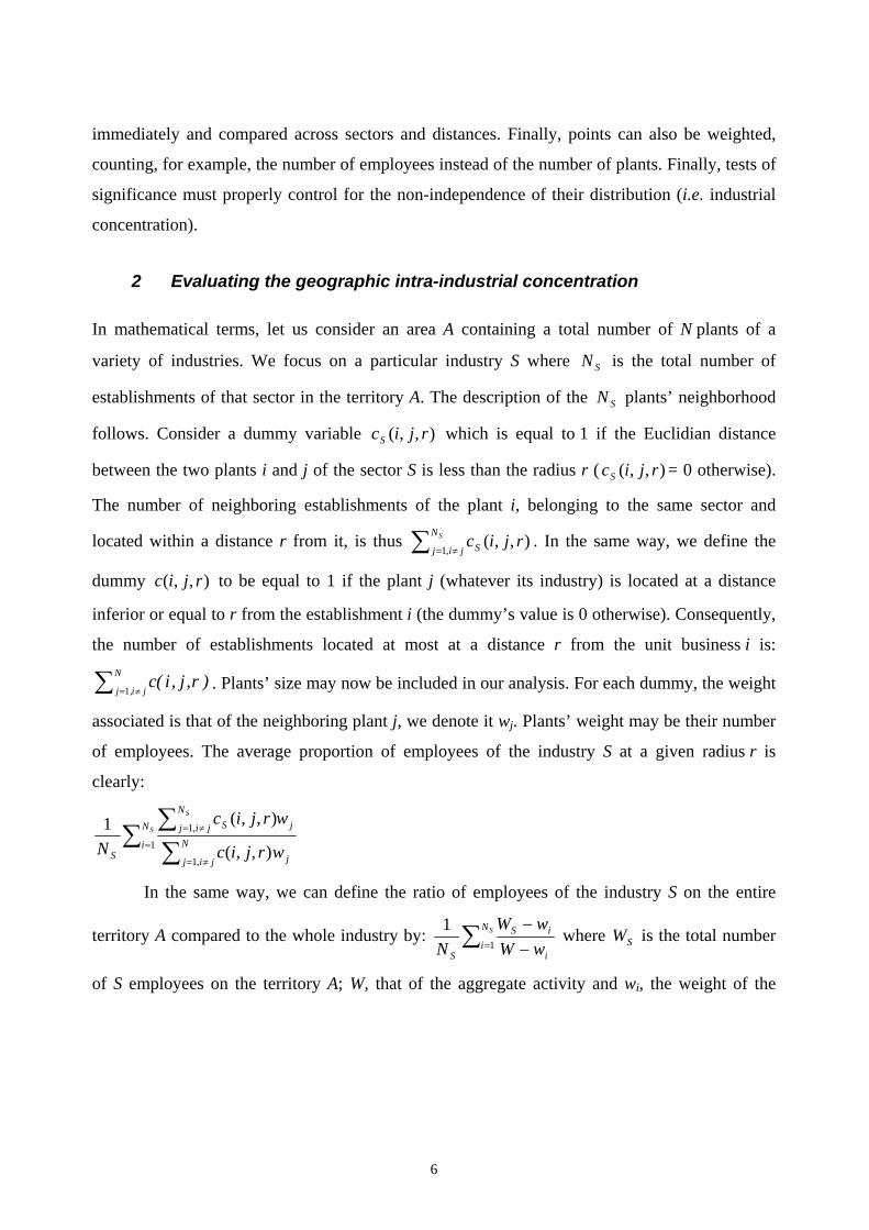
immediately and compared across sectors and distances. Finally, points can also be weighted,

counting, for example, the number of employees instead of the number of plants. Finally, tests of

significance must properly control for the non-independence of their distribution (i.e. industrial

concentration).

2 Evaluating the geographic intra-industrial concentration

In mathematical terms, let us consider an area A containing a total number of N plants of a

variety of industries. We focus on a particular industry S where SN is the total number of

establishments of that sector in the territory A. The description of the SN plants’ neighborhood

follows. Consider a dummy variable ),,( rjicS which is equal to 1 if the Euclidian distance

between the two plants i and j of the sector S is less than the radius r ( ),,( rjicS = 0 otherwise).

The number of neighboring establishments of the plant i, belonging to the same sector and

located within a distance r from it, is thus ∑ ≠=

SN

jij S rjic,1

),,( . In the same way, we define the

dummy ),,( rjic to be equal to 1 if the plant j (whatever its industry) is located at a distance

inferior or equal to r from the establishment i (the dummy’s value is 0 otherwise). Consequently,

the number of establishments located at most at a distance r from the unit business i is:

∑ ≠=

N

ji,j)r,j,i(c

1 . Plants’ size may now be included in our analysis. For each dummy, the weight

associated is that of the neighboring plant j, we denote it wj. Plants’ weight may be their number

of employees. The average proportion of employees of the industry S at a given radius r is

clearly:

∑∑∑

=

≠=

≠=S

S

N

i N

jij j

jN

jij S

S wrjic

wrjic

N 1

,1

,1

),,(

),,(1

In the same way, we can define the ratio of employees of the industry S on the entire

territory A compared to the whole industry by: ∑= −−SN

ii

iS

S wWwW

N 1

1 where SW is the total number

of S employees on the territory A; W, that of the aggregate activity and wi, the weight of the

7

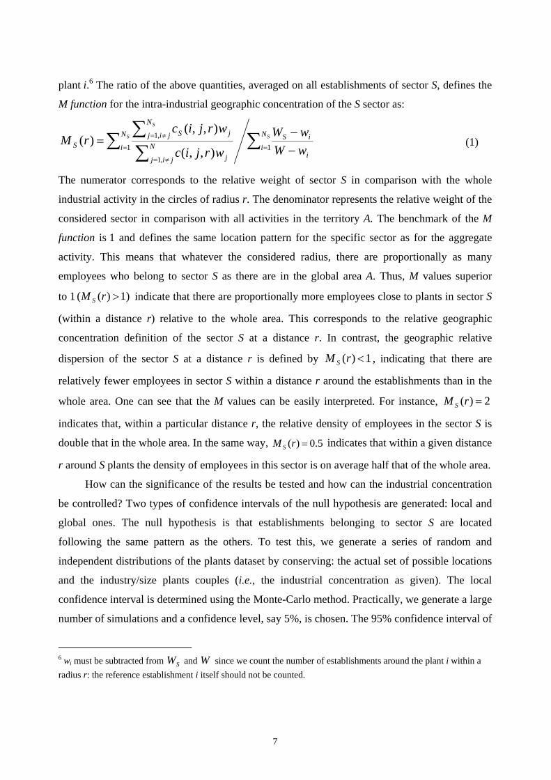
plant i.6 The ratio of the above quantities, averaged on all establishments of sector S, defines the

M function for the intra-industrial geographic concentration of the S sector as:

∑∑∑∑

==

≠=

≠=

−−

= SS

S

N

ii

iSN

i N

jij j

N

jij jSS wW

wWwrjic

wrjicrM

11,1

,1

),,(

),,()( (1)

The numerator corresponds to the relative weight of sector S in comparison with the whole

industrial activity in the circles of radius r. The denominator represents the relative weight of the

considered sector in comparison with all activities in the territory A. The benchmark of the M

function is 1 and defines the same location pattern for the specific sector as for the aggregate

activity. This means that whatever the considered radius, there are proportionally as many

employees who belong to sector S as there are in the global area A. Thus, M values superior

to 1 1))(( >rM S indicate that there are proportionally more employees close to plants in sector S

(within a distance r) relative to the whole area. This corresponds to the relative geographic

concentration definition of the sector S at a distance r. In contrast, the geographic relative

dispersion of the sector S at a distance r is defined by 1)( <rM S , indicating that there are

relatively fewer employees in sector S within a distance r around the establishments than in the

whole area. One can see that the M values can be easily interpreted. For instance, 2)( =rM S

indicates that, within a particular distance r, the relative density of employees in the sector S is

double that in the whole area. In the same way, 0.5)( =rM S indicates that within a given distance

r around S plants the density of employees in this sector is on average half that of the whole area.

How can the significance of the results be tested and how can the industrial concentration

be controlled? Two types of confidence intervals of the null hypothesis are generated: local and

global ones. The null hypothesis is that establishments belonging to sector S are located

following the same pattern as the others. To test this, we generate a series of random and

independent distributions of the plants dataset by conserving: the actual set of possible locations

and the industry/size plants couples (i.e., the industrial concentration as given). The local

confidence interval is determined using the Monte-Carlo method. Practically, we generate a large

number of simulations and a confidence level, say 5%, is chosen. The 95% confidence interval of

6 wi must be subtracted from SW and W since we count the number of establishments around the plant i within a radius r: the reference establishment i itself should not be counted.

8

M function for each value of r is delimited by the outer 5% of the randomly generated values.

Nearly all empirical studies resorting to Ripley’s K function (or one of its extensions) only

compute the local confidence intervals to test the significance of the results. However, Duranton

and Overman (2005) recently criticized the single computation of the local confidence intervals,

considering them as too “optimistic”, and they highlight the need for the global confidence

intervals of the null hypothesis as well. Supposing the values of the M function at different radii

are independently distributed, a proportion of them equal to the confidence threshold is expected

to be outside the confidence interval even though the point process corresponds to the null

hypothesis. For instance at a 5% threshold, complete spatial randomness should not be rejected

when 5 points of a curve made of 100 points leave the confidence interval. Successive values of

Ripley’s functions are actually highly correlated: the risk of erroneous rejection of the null

hypothesis is consequently reduced but cannot be quantified. A global confidence is defined such

that the confidence threshold is the risk that the curve of a function generated by the null

hypothesis exceeds the interval at least once. It may be chosen in many ways but it should have

an equal weight at all distances. A simple method to compute global confidence is by generating

local confidence intervals at increasing confidence levels until the ratio of simulated curves

leaving them reaches the fixed threshold. As an example, suppose that 1,000 curves have been

generated, and the confidence level is fixed to 5%. The outer values at each distance are

eliminated, defining a local confidence interval at 2/1,000 = 0.2%. The curves leaving this

interval are counted. Suppose 10 curves are concerned, the global confidence level is then 1%.

The process is repeated until the threshold is reached. If it is not reached exactly, interpolation is

used.

Five fundamental criteria characterizing a “good” measure of geographic concentration in

economics were presented in the introduction, it should be noted that the M function respects all

of them. Moreover, as we underlined above, an appreciable property of this index is that values

of the M function may be interpreted. Additionally, the M function can be calculated for any

topology. Ripley’s function and its developments (see Goreaud and Pélissier, 1999) require edge-

effect correction for points which are close to borders, so complex geographical shapes are

9

intractable hence the domain is always a polygon or a disc.7 The M function presents an answer

to this problem: comparing the number of neighbors of a certain industry to the number of

neighbors of all establishments in the same area avoids any need for correction. Working on

complex geographical limits, such as a country’s boundaries, is now possible. The last remark

justifies the somewhat complex computation of the M function. Software downloaded from the

authors’ website8 is available in order to facilitate its implementation.

3 Evaluating the co-location of industries

Evaluating the co-location of industries may be interesting if the researcher suspects some

interactions between them. The geographic concentration between industries can be investigated

using the inter-industrial version of the M function which possesses the same properties as the

intra-industrial one. In what follows, we consider the co-location between two sectors denoted S1

and S2. A complete description of the spatial distribution of the co-location patterns of these

industries leads not to one but to two definitions of the M functions. The first one 21,SSM depicts

the spatial structure in non-homogenous space of plants belonging to sector S2 around those of

sector S1. The second function 12 SS ,M describes the spatial structure of plants belonging to

sector S1 around those of sector S2. The meaning of the co-location M functions is thus simple:

we test whether the relative density of employees of one sector located around establishments of

another sector is on average greater or lesser than that on the whole territory.

Let us consider the same territory A and the same notations as used in the previous

section. We now examine the Euclidian distances between plants of two different industries. At

first, we consider the definition of 21,SSM : the reference plants are establishments of the industry

S1 (i.e. those at the centre of the circles). The definition of the co-location )(, 21rM SS function is

7 Sweeney and Feser (1998) fig.1, p.52 or Feser and Sweeney (2000) fig.2, p.361; Pancer-Koteja et al. (1998) fig.1, p.757; Rowlingson and Diggle (1993) fig.5, p.634. 8 http://e.marcon.free.fr/Ripley (English and French versions).

hence:

∑∑∑∑

==

≠=

=

−= 1 21

22

21 11

1

1,

SSS

N

ii

SN

i N

ni,n n

jN

j S

SS wWW

w)r,n,i(c

w)r,j,i(c)r(M (2)

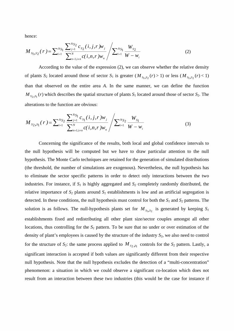
According to the value of the expression (2), we can observe whether the relative density

of plants S2 located around those of sector S1 is greater ( )(, 21rM SS > 1) or less ( )(, 21

rM SS < 1)

than that observed on the entire area A. In the same manner, we can define the function

)(, 12rM SS which describes the spatial structure of plants S1 located around those of sector S2. The

alterations to the function are obvious:

∑∑∑∑

==

≠=

=

−= 2 12

11

12 11

1

1,

SSS

N

ii

SN

i N

ni,n n

N

j jS

SS wWW

w)r,n,i(c

w)r,j,i(c)r(M (3)

Concerning the significance of the results, both local and global confidence intervals to

the null hypothesis will be computed but we have to draw particular attention to the null

hypothesis. The Monte Carlo techniques are retained for the generation of simulated distributions

(the threshold, the number of simulations are exogenous). Nevertheless, the null hypothesis has

to eliminate the sector specific patterns in order to detect only interactions between the two

industries. For instance, if S1 is highly aggregated and S2 completely randomly distributed, the

relative importance of S2 plants around S1 establishments is low and an artificial segregation is

detected. In these conditions, the null hypothesis must control for both the S1 and S2 patterns. The

solution is as follows. The null-hypothesis plants set for 21,SSM is generated by keeping S1

establishments fixed and redistributing all other plant size/sector couples amongst all other

locations, thus controlling for the S1 pattern. To be sure that no under or over estimation of the

density of plant’s employees is caused by the structure of the industry S2, we also need to control

for the structure of S2: the same process applied to 12 SS ,M controls for the S2 pattern. Lastly, a

significant interaction is accepted if both values are significantly different from their respective

null hypothesis. Note that the null hypothesis excludes the detection of a “multi-concentration”

phenomenon: a situation in which we could observe a significant co-location which does not

result from an interaction between these two industries (this would be the case for instance if

11

both industries locate around the plants of another industry). This is undoubtedly a limit of the

inter-industry M function shared with all other distance-based functions.9

III Towards an unified framework on distance-based methods

The incentive of using distance-based methods rather than cluster-based methods is now

well established in the literature. However, the choice of retaining one particular distance-based

method is generally weakly motivated. In what follows, we compare the statistical properties of

distance-based methods and especially those of the two leading geographic concentration

measures namely the Kd and the M function.10 Our aim is to disclose in which cases one measure

should be preferred to another. The heart of our discussion focuses on the implications of using

probability density functions rather than cumulative ones because this remains the main

difference between the Kd and the M function. Surprisingly, the preference of using probability

density function or a cumulative function has never been argued in empirical economic papers.11

The only exception is Duranton and Overman (2005) who claim in the conclusion of their paper

that “K-densities are more informative than [Ripley’s] K-functions with respect to the scale of

localization” without any demonstration. Their idea will be more deeply analyzed hereinafter.

The main conclusion of the advantages/drawbacks comparison is that relative-distance based

measures are generally more complements than substitutes.

1 Common statistical framework

Historically, methods characterizing the structure of point processes as a function of bilateral

distances between pairs of points have been developed by Ripley (1976, 1977).

9 The term co-localisation is employed by Duranton and Overman (2005) if the co-agglomeration indeed results from an attractive pattern of both industries whereas they prefer employing joint-localisation in case of a significant co-agglomeration of both industries occurring for another reason. However, they mention that they can not disentangle empirically from these location patterns. 10 As we underlined in the introduction, the debate for implementing absolute, topographic or relative measures for evaluating the geographic concentration has been recently settled since one of the criteria of a “good” concentration measure states that relative indices must be preferred (Duranton and Overman, 2005; Combes and Overman, 2004). We take this result for granted in our paper. 11 See for instance Fratesi (2008) for an empirical application of the Kd or Arbia and Espa (1996), Barff (1987), Ó hUallacháin and Leslie (2007) and Arbia et al. (2008) for different applications of cumulative distance-based methods.

12

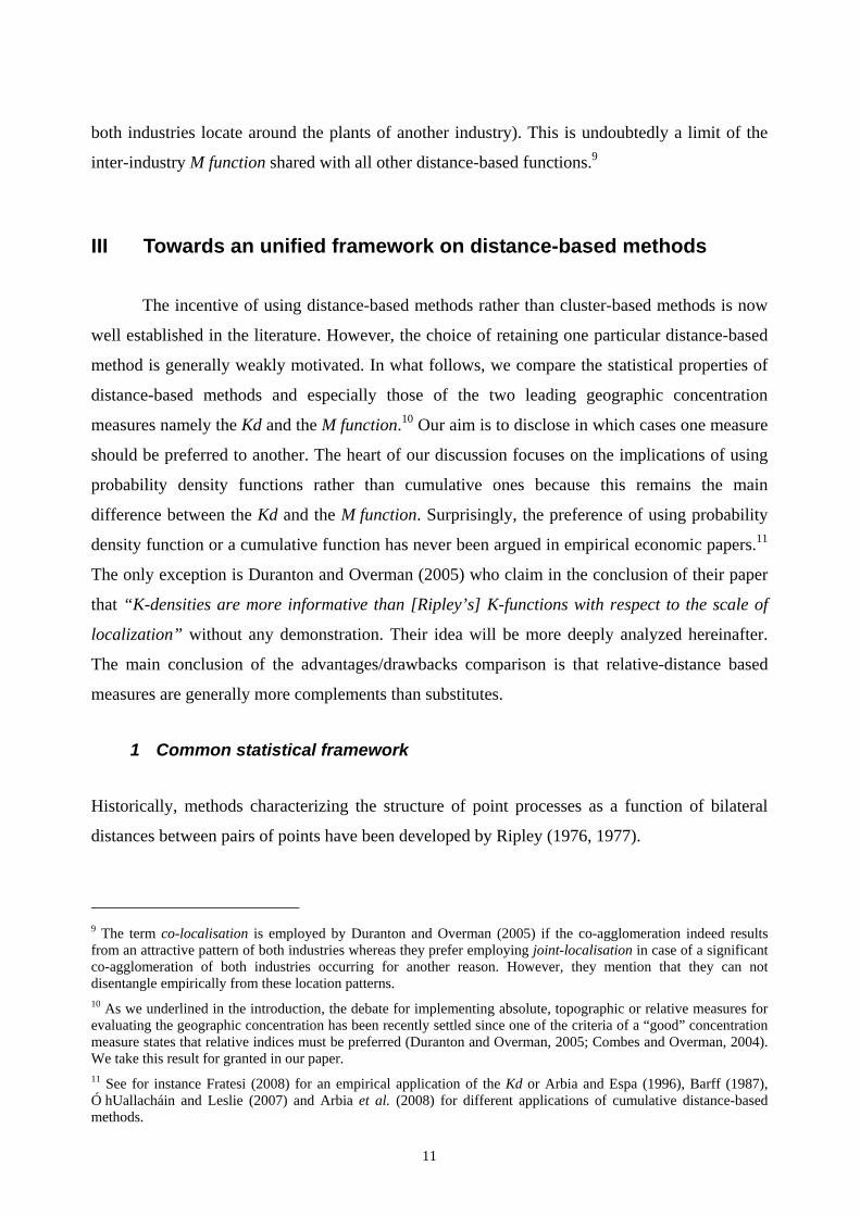
Ripley defined the function ( )rg as the ratio of the probabilities of finding two points at a

distance r from each other to the product of the probabilities of finding each of them. If points

are distributed independently, ( )rg =1; higher values show that point pairs at this distance are

more frequent than under the null hypothesis of independence. The integral function

∫=

=r

dgrK0

2)()(ρ

ρπρρ is easy to estimate.12 Assuming the point density is uniform on an area A

and denoting by N the total number of points on the domain A, we find (Sweeney and Feser,

1998 for example):

∑ ∑−

= >

∧

−=

1

1),,(

)1()( N

i

N

ijrjic

NNArK (4)

In a space where edge effects do not occur (say a torus), ),,( rjic is a dummy: its value

is 1 if the distance between points i and j is less than r. In the real world, it is corrected for edge

effects: when the point i is close to the border of the domain, it has less neighbors because those

outside the domain are not observed. After computing K , )(rg can be estimated by

rrrKrrKrg

ΔΔ−−Δ+

=

∧∧∧

2)()()( , taking rΔ arbitrarily small. g is proportional to the number of

point pairs whose distance is close to r.

K is a cumulative function, while g is a local function. K has been widely used in the

literature, but g has not. Both are restricted to homogenous point processes. To characterize

inhomogenous point sets, to control for the spatial distribution of the whole economy, further

mathematical developments are necessary. Duranton and Overman (2005) chose to define the Kd

function as the probability density function of point-pair distances. Kd is also proportional to the

number of point pairs whose distance is close to r. The differences between Kd and g are: (i) Kd

integrates appropriate smoothing, but this is only a technical improvement, and (ii) Kd does not

correct for any edge effects. Its value is compared to those of point distributions with the same

geometry, which have the same edge effects. We chose another way. From equation 4 and

retaining the same definitions of Ti and T as those given in section II.1., it follows that K can be

rearranged as:

12 For more details, see Marcon and Puech (2003) for a concise presentation of this function.

13

NTN

NTA

NN

r

rjic

rrK

N

i ii

N

i

N

ij

∑∑∑

=

−

=

>∧

=−

= 1

1

1 2

2

1),,(

)( ππ

(5)

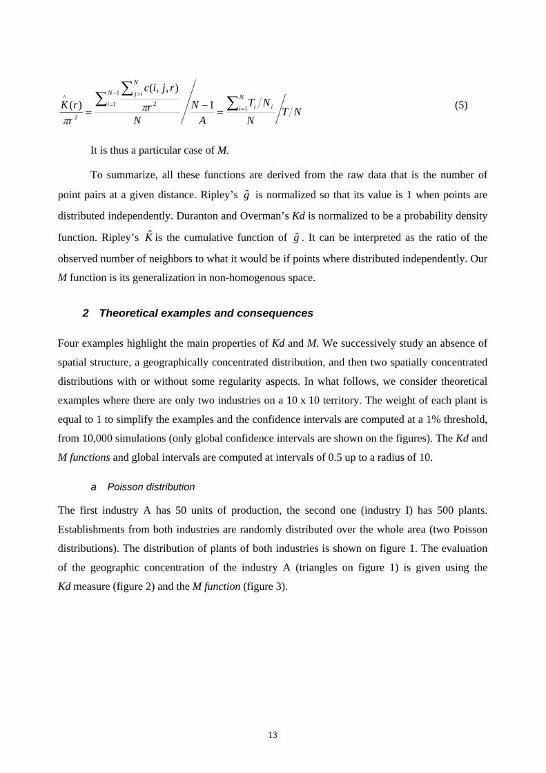
It is thus a particular case of M.

To summarize, all these functions are derived from the raw data that is the number of

point pairs at a given distance. Ripley’s g is normalized so that its value is 1 when points are

distributed independently. Duranton and Overman’s Kd is normalized to be a probability density

function. Ripley’s K is the cumulative function of g . It can be interpreted as the ratio of the

observed number of neighbors to what it would be if points where distributed independently. Our

M function is its generalization in non-homogenous space.

2 Theoretical examples and consequences

Four examples highlight the main properties of Kd and M. We successively study an absence of

spatial structure, a geographically concentrated distribution, and then two spatially concentrated

distributions with or without some regularity aspects. In what follows, we consider theoretical

examples where there are only two industries on a 10 x 10 territory. The weight of each plant is

equal to 1 to simplify the examples and the confidence intervals are computed at a 1% threshold,

from 10,000 simulations (only global confidence intervals are shown on the figures). The Kd and

M functions and global intervals are computed at intervals of 0.5 up to a radius of 10.

a Poisson distribution

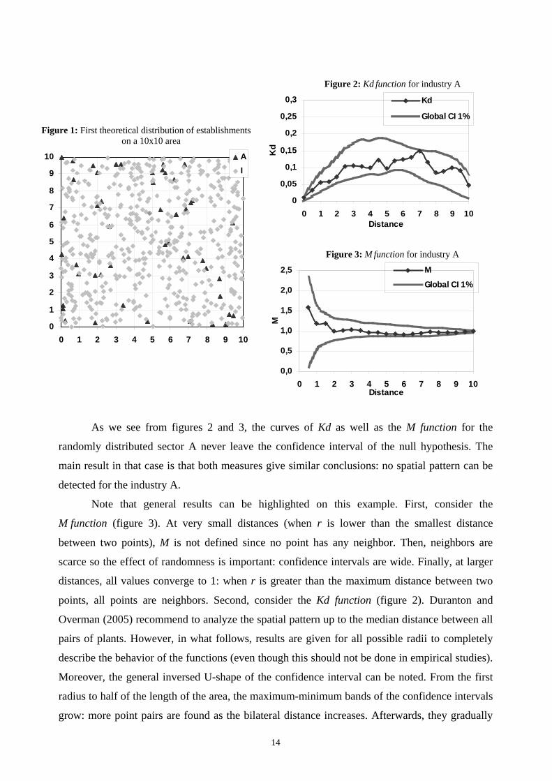
The first industry A has 50 units of production, the second one (industry I) has 500 plants.

Establishments from both industries are randomly distributed over the whole area (two Poisson

distributions). The distribution of plants of both industries is shown on figure 1. The evaluation

of the geographic concentration of the industry A (triangles on figure 1) is given using the

Kd measure (figure 2) and the M function (figure 3).

14

Figure 1: First theoretical distribution of establishments on a 10x10 area

0

1

2

3

4

5

6

7

8

9

10

0 1 2 3 4 5 6 7 8 9 10

AI

Figure 2: Kd function for industry A

0

0,05

0,1

0,15

0,2

0,25

0,3

0 1 2 3 4 5 6 7 8 9 10Distance

Kd

Kd

Global CI 1%

Figure 3: M function for industry A

0,0

0,5

1,0

1,5

2,0

2,5

0 1 2 3 4 5 6 7 8 9 10Distance

MM

Global CI 1%

As we see from figures 2 and 3, the curves of Kd as well as the M function for the

randomly distributed sector A never leave the confidence interval of the null hypothesis. The

main result in that case is that both measures give similar conclusions: no spatial pattern can be

detected for the industry A.

Note that general results can be highlighted on this example. First, consider the

M function (figure 3). At very small distances (when r is lower than the smallest distance

between two points), M is not defined since no point has any neighbor. Then, neighbors are

scarce so the effect of randomness is important: confidence intervals are wide. Finally, at larger

distances, all values converge to 1: when r is greater than the maximum distance between two

points, all points are neighbors. Second, consider the Kd function (figure 2). Duranton and

Overman (2005) recommend to analyze the spatial pattern up to the median distance between all

pairs of plants. However, in what follows, results are given for all possible radii to completely

describe the behavior of the functions (even though this should not be done in empirical studies).

Moreover, the general inversed U-shape of the confidence interval can be noted. From the first

radius to half of the length of the area, the maximum-minimum bands of the confidence intervals

grow: more point pairs are found as the bilateral distance increases. Afterwards, they gradually

15

decrease and return to zero: edge effects get more importance with distance until no neighbor can

be found because they would have to be outside the domain.

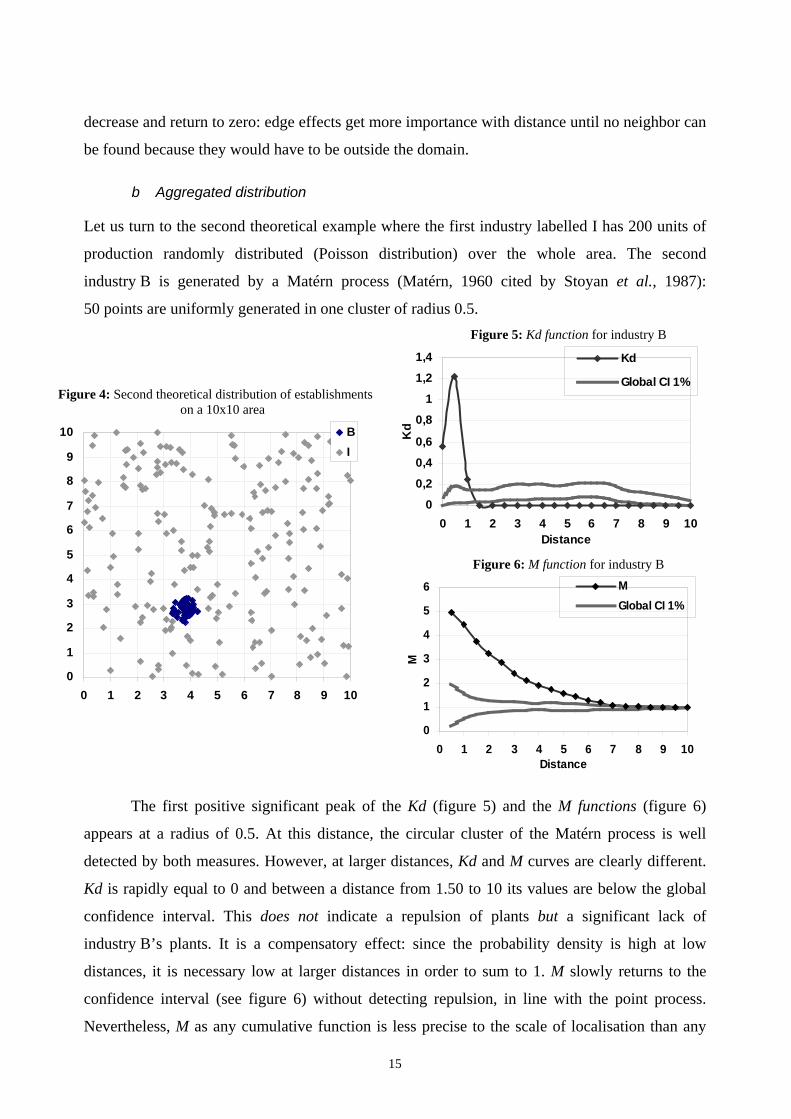
b Aggregated distribution

Let us turn to the second theoretical example where the first industry labelled I has 200 units of

production randomly distributed (Poisson distribution) over the whole area. The second

industry B is generated by a Matérn process (Matérn, 1960 cited by Stoyan et al., 1987):

50 points are uniformly generated in one cluster of radius 0.5.

Figure 4: Second theoretical distribution of establishments on a 10x10 area

0

1

2

3

4

5

6

7

8

9

10

0 1 2 3 4 5 6 7 8 9 10

BI

Figure 5: Kd function for industry B

0

0,2

0,4

0,6

0,8

1

1,2

1,4

0 1 2 3 4 5 6 7 8 9 10Distance

Kd

Kd

Global CI 1%

Figure 6: M function for industry B

0

1

2

3

4

5

6

0 1 2 3 4 5 6 7 8 9 10Distance

M

M Global CI 1%

The first positive significant peak of the Kd (figure 5) and the M functions (figure 6)

appears at a radius of 0.5. At this distance, the circular cluster of the Matérn process is well

detected by both measures. However, at larger distances, Kd and M curves are clearly different.

Kd is rapidly equal to 0 and between a distance from 1.50 to 10 its values are below the global

confidence interval. This does not indicate a repulsion of plants but a significant lack of

industry B’s plants. It is a compensatory effect: since the probability density is high at low

distances, it is necessary low at larger distances in order to sum to 1. M slowly returns to the

confidence interval (see figure 6) without detecting repulsion, in line with the point process.

Nevertheless, M as any cumulative function is less precise to the scale of localisation than any

16

probability density function (including the Kd function). Some imprecision on the plants

distribution analysis emerge here because M returns gradually and not suddenly inside the

confidence interval bands (even if there are no industry B neighbors’ after a radius of 0.5). Both

functions give pertinent and complementary information on the spatial structure.

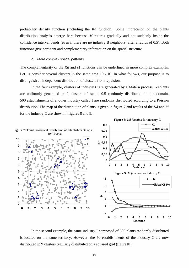
c More complex spatial patterns

The complementarity of the Kd and M functions can be underlined in more complex examples.

Let us consider several clusters in the same area 10 x 10. In what follows, our purpose is to

distinguish an independent distribution of clusters from repulsion.

In the first example, clusters of industry C are generated by a Matérn process: 50 plants

are uniformly generated in 9 clusters of radius 0.5 randomly distributed on the domain.

500 establishments of another industry called I are randomly distributed according to a Poisson

distribution. The map of the distribution of plants is given in figure 7 and results of the Kd and M

for the industry C are shown in figures 8 and 9.

Figure 7: Third theoretical distribution of establishments on a 10x10 area

0

1

2

3

4

5

6

7

8

9

10

0 1 2 3 4 5 6 7 8 9 10

CI

Figure 8: Kd function for industry C

0

0,05

0,1

0,15

0,2

0,25

0,3

0 1 2 3 4 5 6 7 8 9 10Distance

Kd

KdGlobal CI 1%

Figure 9: M function for industry C

0

1

2

3

4

5

0 1 2 3 4 5 6 7 8 9 10Distance

M

M

Global CI 1%

In the second example, the same industry I composed of 500 plants randomly distributed

is located on the same territory. However, the 50 establishments of the industry C are now

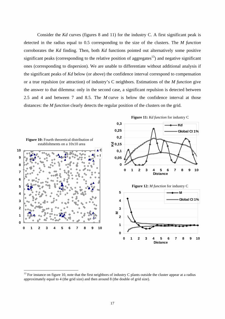
distributed in 9 clusters regularly distributed on a squared grid (figure10).

17

Consider the Kd curves (figures 8 and 11) for the industry C. A first significant peak is

detected in the radius equal to 0.5 corresponding to the size of the clusters. The M function

corroborates the Kd finding. Then, both Kd functions pointed out alternatively some positive

significant peaks (corresponding to the relative position of aggregates13) and negative significant

ones (corresponding to dispersion). We are unable to differentiate without additional analysis if

the significant peaks of Kd below (or above) the confidence interval correspond to compensation

or a true repulsion (or attraction) of industry’s C neighbors. Estimations of the M function give

the answer to that dilemma: only in the second case, a significant repulsion is detected between

2.5 and 4 and between 7 and 8.5. The M curve is below the confidence interval at those

distances: the M function clearly detects the regular position of the clusters on the grid.

Figure 10: Fourth theoretical distribution of establishments on a 10x10 area

0

1

2

3

4

5

6

7

8

9

10

0 1 2 3 4 5 6 7 8 9 10

CI

Figure 11: Kd function for industry C

0

0,05

0,1

0,15

0,2

0,25

0,3

0 1 2 3 4 5 6 7 8 9 10Distance

Kd

Kd

Global CI 1%

Figure 12: M function for industry C

0

1

2

3

4

5

0 1 2 3 4 5 6 7 8 9 10Distance

M

M

Global CI 1%

13 For instance on figure 10, note that the first neighbors of industry C plants outside the cluster appear at a radius approximately equal to 4 (the grid size) and then around 8 (the double of grid size).

What can we learn from those examples? First, the Kd and M measures present some

advantages and drawbacks in the evaluation of spatial structures. Secondly, they seem more

complementary than substitutable. On the one hand, the Kd function shows the excess or the lack

of neighbors that M can not systematically detect. On the other hand, the M function evaluates

the cumulated effects of successive patterns and can distinguish compensation from opposite

strength (see the last two examples of the section).

IV Conclusion

The aim of this paper was to improve some existing relative statistical tools to test the spatial

concentration of industries. We present evidence that M functions constitute first-class

instruments to evaluate the intra- or inter-industrial geographic concentration. Nonetheless, some

intrinsic limits of these new tools suggest different research agendas to fill the gap between the

theoretical and empirical literatures. Despite the considerable recent interest of researchers in an

“ideal” concentration index and even if significant progress has been made, work still needs to be

done to bridge the last two criteria, the most difficult to respect: the complete integration of the

tools to economic theory and the independence of geographic concentration measures to the

industrial classification (Combes and Overman, 2004). In this paper, we have enhanced existing

distance-based methods but further investigations are still required.

19

References

Arbia G. and G.Espa (1996). Statistica economica territoriale. Cedam, Padua. Arbia G., Espa G. and D.Quah (2008). A class of spatial econometric methods in the empirical analysis of clusters of firms in the space. Empirical Economics 34: 81-103.

Barff, R. A. (1987). Industrial Clustering and the Organization of Production: A Point Pattern Analysis of Manufacturing in Cincinnati, Ohio. Annals of the Association of American Geographers 77: 89-103.

Besag J.E. (1977). Comments on Ripley's paper, Journal of the Royal Statistical Society B 39: 193-195.

Briant A., Combes P.-P., and M. Lafourcade (2008). Dots to boxes: Do the size and shape of spatial units jeopardize economic geography estimations? CEPR Discussion Paper No 6928.

Combes P.-P., and H. Overman (2004). The spatial distribution of economic activities in the European Union. in: J.V. Henderson, and J.-F. Thisse, (Eds.), Handbook of Urban and Regional Economics, Elsevier. North Holland, Amsterdam.

Duranton G. and H.G. Overman (2005). Testing for Localisation Using Micro-Geographic Data. Review of Economic Studies 72: 1077-1106.

Duranton G. and H.G. Overman (2008). Exploring the Detailed Location Patterns of UK Manufacturing Industries using Microgeographic Data. Journal of Regional Science 48: 213-243.

Feser E.J. and S.H. Sweeney (2000). A test for the coincident economic and spatial clustering of business enterprises. Journal of Geographical Systems 2: 349-373.

Fratesi U. (2008). Issues in the measurement of localization. Environment and Planning A 40: 733-758.

Fujita M. and J.-F. Thisse (2002). Economics of Agglomeration: Cities, Industrial Location and Regional Growth, Cambridge University Press, New York.

Goreaud, F. and R. Pélissier (1999). On explicit formulas of edge effect correction for Ripley’s K-function. Journal of Vegetation Science 10: 433-438.

Haaland, J. I., Kind, H. J., Midelfart-Knarvik, K. H. and J. Torstensson (1999). What determines the economic geography of Europe? Centre for Economic Policy Research. Discussion paper, 2072.

Krugman P. (1991). Geography and Trade, MIT Press, London.

Marcon E. and F. Puech (2003). Evaluating the Geographic Concentration of Industries Using Distance-Based Methods. Journal of Economic Geography 3: 409-428.

Marcon, E. and Puech, F. (2005). The determinants of agglomeration in a continuous-space framework. Mimeo.

Marshall A. (1890). Principle of Economics, Macmillan, London.

Matérn B. (1960). Spatial variation. Meddelanden från Statens Skogsforskningsinstitut 49: 1-144.

20

Mori T., Nishikimi K. and T.E. Smith (2005). A divergence statistic for industrial localization. Review of Economics and Statistics 87: 635-651.

Morphet C.S. (1997); A statistical method for the identification of spatial clusters. Environment and Planning A 29: 1039-1055.

Ó hUallacháin B. and T.F. Leslie (2007), Producer Services in the Urban Core and Suburbs of Phoenix, Arizona. Urban Studies 44: 1581-1601.

Pancer-Koteja E., Szwagrzyk J. and J. Bodziarczyk (1998). Small-scale spatial pattern and size structure of Rubus hirtus in a canopy gap. Journal of Vegetation Science 9: 755-762.

Puech F. (2003). Concentration géographique des activités industrielles : Mesures et enjeux, Ph.D. Thesis, Université de Paris I, Panthéon-Sorbonne, Paris.

Ripley B.D. (1976). The Second-Order Analysis of Stationary Point Processes. Journal of Applied Probability 13: 255-266.

Ripley B.D. (1977). Modelling Spatial Patterns. Journal of the Royal Statistical Society B 39: 172-212.

Rosenthal S.S. and W.C. Strange (2003). Geography, Industrial Organisation, and Agglomeration. Review of Economics and Statistics 85: 377-393.

Rosenthal S.S. and W.C. Strange (2004). Evidence on the Nature and Sources of Agglomeration Economies. in: J.V. Henderson, and J.-F. Thisse, (Eds.), Handbook of Urban and Regional Economics, Elsevier. North Holland, Amsterdam.

Rowlingson B.S. and P.J. Diggle (1993). SPLANCS: Spatial Point Pattern Analysis Code in S-Plus. Computers & Geosciences 19: 627-655.

Stoyan D., Kendal W.S. and J. Mecke (1987); Stochastic Geometry and its Applications, John Wiley & Sons, New York.

Sweeney S.H. and E.J. Feser (1998). Plant Size and Clustering of Manufacturing Activity. Geographical Analysis 30: 45-64.

Weber A. (1909). Uber den Standort der Industrien, Russell & Russell, Tübingen.