measurements of satisfaction in the real...
TRANSCRIPT
MEASUREMENTS OF SATISFACTION
IN THE
REAL ESTATE BUSINESS
By John Vestergaard Olesen
A PhD thesis submitted to
School of Business and Social Sciences, Aarhus University,
in partial fulfilment of the requirements of
the PhD degree in
Business Administration
July 2015

I. Acknowledgements
There are many people to whom I am very grateful and owe a large debt of gratitude. A very special
thanks to Peder Østergaard for initiating the process, to Kai Kristensen for assisting me in the early
stages of the process, to Mogens Dilling-Hansen for being there through the whole journey and to
Jacob Eskildsen for his dedication to helping me succeed. My deepest and warmest thanks go out to
you all for your time, support, guidance, ideas and sharp minds.
I also owe thanks to my colleagues at the Department of Business Development and Technology
(BTECH) and ICOA for their advice and interest in the project, and a very special thanks to our
department secretary, Lisa Vestergaard Sørensen, for keeping me in order and for the careful
proofreading of this dissertation.
I am also very grateful to Forskningsfonden for Midt- and Vestjylland and BTECH for making this
whole journey possible.
Finally, and most importantly, thanks to the people around me. To my parents, Tytte and Bent, for
your unconditional love, for giving me all the opportunities that you have, for always being there
and for showing me by example how to be a good human being – you will always be in my heart,
wherever you are. To my beautiful love and wife, Bente, and our two wonderful children, Natalie
and Daniel – I love you all for bringing endless love, joy and meaning into my life.
“Sometimes the fastest way to get there is to go slow”
Tina Dickow

II. Introduction
Since its introduction by Karl Jöreskog in 1973, the covariance-based approach to conducting
structural equation modelling (CB-SEM) has been the subject of substantial interest among
empirical researchers across practically all social science disciplines as well as the preferred way of
performing SEM. However, over the last decade, the use of Herman Wold’s variance-based partial
least squares alternative, PLS-SEM, (Wold, 1982) has increased dramatically (Hair et al., 2012),
and it is now a key research method. This PhD thesis, composed of five self-contained papers,
continues along that path and uses PLS-SEM in estimation of simple as well as rather complex
models.
Data for paper 1-3 have been collected in cooperation with one of the largest real estate chains in
Denmark. The data collection was carried out in mid-June 2012 among customers who had sold real
estate through the chain within the last 12 months. Via email, the customers were encouraged to
participate in the survey by clicking a link that took them to an online questionnaire
In addition to some concomitant variables, which were to be used to characterise the detected latent
segments, the questionnaire consisted of 30 questions covering the EPSI part as well as 3 questions
addressing each of the 5 SERVQUAL dimensions. Supported by findings in Cronin et al. (1992),
Brown et al. (1993), McAlexander et al. (1994) and Durvasula et al. (1999), only manifest variables
related to perception were included in the 5*3 SERVQUAL questions. Following the
recommendations in Kristensen et al. (2009) and the tradition within the EPSI measurements, while
deviating from the traditional SERVQUAL gap measurement in Parasuraman et al. (1988), all the
EPSI questions as well as the SERVQUAL questions have been answered according to a 10-item
scale.
The email was sent to 2,800 customers, 442 of whom clicked the survey link. Of the 442
respondents, 326 had answered all 30 EPSI questions, but a few had failed to answer all 15
SERVQUAL questions. Seeing that the EM and regression substitution (Brown, 1994; Olinsky et
al., 2003) are preferred to pairwise deletion and mean substitution in general, and in customer
satisfaction analyses, as in a PLS model, in particular (Kristensen et al., 2009), and seeing that the
inclination is to prefer the EM substitution to the regression-based substitution, the EM algorithm is

used to fill the few holes in the dataset, which, accordingly, consists of a complete set of 326
respondents on all 30 EPSI and 15 SERVQUAL questions.
Paper 4 and 5 address an adjusted EPSI model that can be applied to dyadic data in businesses
where we operate with a “buyer” and a “seller” on each side of an agent, implying that the
satisfaction becomes multidimensional. Paper 4 is a conceptual paper, while paper 5 is a simulation
study in which the focus is on the three factors of sample size: n = [50; 100; 250; 1000], number of
manifest indicators: p = [2; 4; 6] and standard deviation on the error terms in the measurement
model: 𝜎𝜀= [1; 5; 10; 20]. A full factorial design with three factors in 3 ∙ 4 ∙ 4 = 48 runs, giving a
total of 16,800 “pairs of respondents” and a total of 806,400 values of manifest variables were
completed, and the models’ ability to reproduce the parameters were investigated .
III. Summary of the thesis
Paper 1: Real Estate Agent Satisfaction – A City in Denmark?
Presented on Symposium in Applied Statistics, 2013
Published in Symposium i Anvendt Statistik, 2013, ISBN 978-87-501-2054-4
No academic studies have tested the structure of the EPSI model on an extremely low-frequency
market, so in this study, we demonstrate how the real estate business behaves when subjected to a
traditional EPSI measurement. The model does not differ substantially from measurements in
traditional businesses. All the path coefficients exhibit the expected signs, and the survey has
managed to create a reliable and valid benchmark for the Danish real estate business.
Paper 2: The Integration of SERVQUAL into a Customer Satisfaction Index – A Case Study
from the Danish Real Estate Business
Submitted to Journal of Real Estate Research
This study examines the interplay between the SERVQUAL model and a customer satisfaction
index. The findings indicate that the five classic SERVQUAL dimensions can be integrated into a
national customer satisfaction index, that the framework will benefit from the inclusion of the
SERVQUAL dimensions and that this inclusion in no way will affect traceability. When comparing
the EPSI scores with indices from a new model, we see that the differences are quite small. This
suggests that introducing SERVQUAL dimensions into the EPSI model means that no traceability
is lost. It seems that reliability, responsiveness and empathy are the most promising dimensions, but
the SERVQUAL dimensions work differently in different segments. For both genders, empathy is
significant. Furthermore, also the other “soft” dimension, responsiveness, is very important to
women. This is not the case for men, who, on the other hand, appreciate reliability, assurance and
tangibles. So even though assurance and tangibles are insignificant in the complete model, all five
SERVQUAL dimensions are at least significant in one gender submodel.

Paper 3: Loyalty-Based Segmentation – The Use of REBUS-PLS and EPSI Measurement in
an Extremely Low-Frequent Transaction
Submitted to Journal of Real Estate Literature
Little research has been conducted on the performance of the response-based algorithm for
performing unit segmentation, REBUS-PLS, on complex models. This study demonstrates that
REBUS-PLS, also in a complex structural equation model such as a modified EPSI model, is able
to detect unobserved heterogeneity and identify two segments with differing models. The article
also suggests that a new threshold for GoF improvement is needed in well-performing models: The
fit of the global model is 0.857; thus, it is worth noting that these segments would have remained
undetected if we insisted on a GoF improvement of at least 25%, as originally suggested by
Trinchera (2007).
As concerning the five SERVQUAL dimensions, reliability, responsiveness and empathy were
significant in explaining the EPSI service in the global model, and responsiveness, empathy and
tangibles appeared to be significant in one of the local models, while reliability and responsiveness
were significant in the other segment. The alternating conclusions concerning the existence of the
SERVQUAL dimensions in the real estate business (McDaniel et al., 1994; Seiler et al., 2000;
Seiler et al., 2008) can now be seen as a result of the existence of different segments.
Paper 4: EPSI Measurement on Agent Performance
Co-written with Jacob Kjær Eskildsen
Presented on the PMA conference Designing the High-Performing Organization, June 25-27, 2014
Even though the real estate agent is the seller’s agent, he must also take measures to satisfy the
buyer, thus ensuring that he is in commission to sell and possibly also resell the property in the
future. Accordingly, the real estate agent faces the challenge of being able to simultaneously secure
a higher satisfaction level among both the buyer and the seller. As a result, in the real estate
business, the satisfaction concept becomes multidimensional at the latent level, which entails some
interesting challenges for the traditional EPSI model. In this conceptual paper, we have taken the
first steps towards a model that can be used in satisfaction studies in businesses where we, in the
minefield between two types of customers, have a broker with the task to make both ends meet.

Paper 5: EPSI Measurement on Dual Businesses
Submitted to Total Quality Management & Business Excellence
In this paper, we take a deeper look at the adjusted EPSI model from paper 4 – a model that can be
applied in businesses characterised by having a broker with the task of making both ends meet in
the minefield between two types of customers. A structural equation model that can be applied to
customer satisfaction data in these businesses where the satisfaction and loyalty dimensions are
multidimensional has been proposed, and the quality of PLS estimation when applied on simulated
data has been investigated.
The study focuses on the three factors of sample size, number of manifest variables and standard
deviation on the error terms in the measurement model and the levels n = [50; 100; 250; 1000], p =
[2; 4; 6] and 𝜎𝜀= [1; 5; 10; 20], respectively. Findings are that, all in all, despite its high complexity,
the model roughly behaves as expected. Consistency at large and the importance of low indicator
reliability in the constructs are very conspicuous, stressing the significance for the practitioners to
formulate questions with as low a standard deviation as possible. In terms of the sample size, the
simulation study suggests that sample sizes of 100 are sufficient to ensure a reasonable level of bias
of the path coefficients in the model – a very useful result, partly since we in some of the affected
industries will struggle to find respondents, and partly since we need “seller”-“buyer” pairs and not
only a number of “buyers” and “sellers”.
IV. Summary in Danish
Denne afhandling består af fem selvstændige artikler. De kredser alle om anvendelsen af
strukturelle ligningsmodeller på tilfredshedsmodeller inden for ejendomsmæglerbranchen. Denne
branche er særligt interessant af to årsager: dels er der tale om en ekstremt lavfrekvent handling
omkring en stor økonomisk beslutning, og dels er branchen jo kendetegnet ved, at mægleren
befinder sig i minefeltet med to slags kunder – nemlig sælger og køber.
Artikel 1: Real Estate Agent Satisfaction –A City in Denmark?
Præsenteret på Symposium i Anvendt Statistik, 2013
Offentliggjort i Symposium i Anvendt Statistik, 2013, ISBN 978-87-501-2054-4
Dette studie er det første til at undersøge, hvorledes strukturen af den traditionelle EPSI-model ser
ud, hvis den anvendes på et ekstremt lavfrekvent område. I dette papir påvises, at EPSI-modellen
tilsyneladende også er anvendelig, hvis den anvendes på ejendomsmæglermarkedet. Den afviger
ikke substantielt fra målinger foretaget i mere traditionelle brancher: stikoefficienterne har alle de
forventede tegn, kvaliteten af modellen er god, målt på en forklaringsgrad på tilfredshedsvariablen
på 85 %, og der er ved undersøgelsen lavet reliable og valide benchmarks for den danske
ejendomsmæglerbranche.
Artikel 2: The Integration of SERVQUAL into a Customer Satisfaction Index – A Case Study
from the Danish Real Estate Business
Indsendt til Journal of Real Estate Research
I denne artikel undersøges samspillet mellem de klassiske SERVQUAL-dimensioner og
kundetilfredshedsindekset hentet fra EPSI-modellen. Resultaterne antyder, at SERVQUAL-
dimensionerne med fordel kan integreres i EPSI-modellen. Ved at sammenligne EPSI-scoren fra
den klassiske model med fire eksogene og tre endogene dimensioner med de tilsvarende scores fra
en ny model med otte eksogene og fire endogene dimensioner noterer vi os, at diskrepanserne er
meget små, således at vi ved at skifte til en ny model ikke mister nogen ”traceabilitet”. Det er i
særlig grad reliability-, responsiveness-, og empathy-dimensionerne, der er de mest lovende, men vi

ser også, at SERVQUAL-dimensionerne opfører sig forskelligt i forskellige segmenter. Empathy er
signifikant for begge køn, mens den anden ”bløde” dimension, responsiveness, kun er signifikant
for kvinder. For mændenes vedkommende er det desuden reliability, assurance og tangibles, der
betyder noget. Selv om assurance og tangibles således er insignifikante i modellen anvendt på det
fulde datasæt, ser vi altså, at alle fem SERVQUAL-dimensioner mindst er signifikante i en
undermodel.
Artikel 3: Loyalty-Based Segmentation – The Use of REBUS-PLS and EPSI Measurement in
an Extremely Low-Frequent Transaction
Indsendt til Journal of Real Estate Literature
Der har kun været forsket ganske lidt i, hvorledes den responsbaserede algoritme til at foretage
enhedssegmentering, REBUS-PLS, virker på komplekse modeller. Denne artikel demonstrerer, at
REBUS-PLS, også i komplekse strukturelle modeller såsom den modificerede EPSI-model, er i
stand til at opdage ikke-observeret heterogenitet og finde to segmenter med forskellige modeller. I
artiklen foreslås en ny tærskelværdi for GoF-forbedringen til brug for modeller med en i forvejen
høj GoF-værdi: Den globale models fit er således 0,857, hvilket umuliggør en forbedring på 25 %,
som oprindeligt foreslået af Trinchera (2007).
Med hensyn til de fem SERVQUAL-dimensioner er reliability, responsiveness og empathy
signifikant forklarende for EPSI-servicedimensionen, mens responsiveness, empathy og tangibles er
signifikante i den ene lokale model, mens reliability og responsiveness er signifikante for det andet
segment. De forskellige konklusioner i litteraturen mht. eksistensen af SERVQUAL-dimensionerne
inden for ejendomsmæglerbranchen (McDaniel et al., 1994; Seiler et al., 2000; Seiler et al., 2008)
kan således nu ses som et resultat af eksistensen af forskellige segmenter.
Artikel 4: EPSI Measurement on Agent Performance
Fælles med Jacob Kjær Eskildsen.
Præsenteret på PMA-konferencen Designing the High-Performing Organization, juni 25-27, 2014
Selv om den klassiske ejendomsmægler som udgangspunkt er ”sælgers mand”, ligger der også et
stort arbejde i at tilfredsstille køber – dels for at sikre, at der i det hele taget kommer en handel, men

også for at sælger skal blive så loyal, at han benytter den same ejendomsmægler, når ejendommen
atter skal sælges. Mægleren står dermed med den udfordring, at han skal opnå en simultan høj
tilfredshed på begge sider af bordet – to sider, der som udgangspunkt kan have modsatrettede
interesser for så vidt angår pris og øvrige betingelser. Tilfredshedsbegrebet er derfor
multidimensionalt på det latente niveau, hvilket giver en række udfordringer for den klassiske EPSI-
model. I dette konceptuelle papir har vi taget de første skridt mod en tilfredshedsmodel, der kan
benyttes, når en agent skal forsøge at få enderne til at mødes i minefeltet mellem en sælger og
køber, afsender og modtager eller offer og anklaget.
Artikel 5: EPSI Measurement on Dual Businesses
Indsendt til Total Quality Management & Business Excellence
I dette simulationsstudie opnår vi en dybere forståelse for den i artikel 4 opstillede
tilfredshedsmodel til estimering af simultan køber- og sælgertilfredshed i forretningsområder, der
simultant opererer med to slags kunder ved at undersøge kvaliteten af PLS-estimering på
simulerede data.
Fokus er på de følgende tre faktorer: Stikprøvestørrelse, antallet af manifeste variable samt
standardafvigelsen på fejlleddet i den ydre model, og niveauerne var sat til henholdsvis n = [50;
100; 250; 1000], p = [2; 4; 6] og σε= [1; 5; 10; 20]. Konklusionerne er, at modellen, på trods af sin
høje grad af kompleksitet, i store træk opfører sig som forventet. Consistency at large og
vigtigheden af lav indikatorreliabilitet i de enkelte dimensioner er meget tydelig og understreger,
hvor vigtigt det i spørgeskemaundersøgelser er at formulere spørgsmål med så lav en
standardafvigelse som muligt. Med hensyn til stikprøvestørrelsen viser studiet, at en størrelse på
100 er tilstrækkelig for at sikre en rimelig grad af bias på modellens stikoefficienter – et meget
vigtigt resultat, dels fordi vi i nogle af de berørte brancher vil få vanskeligt ved at finde mange
respondenter, og dels fordi vi er nødt til at finde ”køber/sælger”-par og ikke blot en række ”købere”
og en række ”sælgere”.

References
Brown, T. J., Churchill, G.A. & Peter, J.P., 1993: Research note: improving the measurement of
service quality, Journal of Retailing, 69: 1, pp. 127-39.
Brown, R.L., 1994: Efficacy of the indirect approach for estimating structural equation models with
missing data: A comparison of five methods. Structural Equation Modeling, 1, 287-316.
Cronin, J. J., Taylor, S.A., 1992: Measuring Service Quality: A Reexamination and extension,
Journal of Marketing, July 1992, 56, pp. 55-68.
Durvasula, S., Lysonski, S. and Mehta, S.C., 1999: Testing the SERVQUAL scale in the business-
to-business sector: the case of ocean freight shipping service, Journal of Services Marketing, 13:2,
pp. 132-50.
Hair, J., Sarstedt, M., Ringle, C.M. and. Mena, J., 2012: An assessment of the use of partial least
squares structural equation modeling in marketing research, Journal of the Acad. Mark. Sci. (2012)
40:414-433.
Kristensen, K., Eskildsen, J., 2009: “Design of PLS-satisfaction studies, In Handbook of Partial
Least Squares: Concepts, Methods and Applications in Marketing and Relates fields, Springer
Handbooks of Computational Statistics, eds. V.E.Vinzi, W.W.Chin, J.Henseler and H.Wang:
Springer Verlag.
McAlexander, J.H., Kaldenberg, D.O. & Koenig, H.F., 1994: Service quality measurement:
examination of dental practices sheds more light on the relationships between service quality,
satisfaction, and purchase intensions in a health care setting, Journal of Health Care Marketing,
14:3, pp. 34-40.
McDaniel, J., M. Louargand, 1994: Real estate brokerage service quality: An examination, Journal
of Real Estate Research, 1994, 9:3, 339-351.
Olinsky, A., Chen, S. & Harlow, L., 2003: The comparative efficacy of imputation methods for
missing data in structural equation modelling, European Journal of Operational Research, 151, pp.
53-79.
Parasuraman, A. Zeithaml, V.A. and Berry, L.L. 1988: SERVQUAL: A multi-item scale for
measuring consumer perceptions of service quality, Journal of Retail, 64: 1, pp. 12-40.
Seiler, V.; J. Webb, T. Whipple, 2000: Assessment of real estate brokerage service quality with a
practicing professional instrument, Journal of real estate research, 2000, 20:1/2, p. 105-117.
Seiler, V.; M. Seiler, D. Winkler, G. Newell, J. Webb, 2008: Service quality dimensions in
residential real estate brokerage, Journal of housing research, 2008, 17: 2, 101-116.
Trinchera, L., 2007: Unobserved Heterogeneity in Structural Equation Models: a new approach to
latent class detection in PLS Path Modeling. PhD, Università degli Studi di Napoli Federico II.
Wold, H., 1982: Soft Modeling: The basic design and some extensions, in In K.G. Jöreskog &
H.Wold (Eds.), Systems under direct observations (pp.263-270), New York: North Holland, 1982.
Real Estate Agent Satisfaction –
A City in Denmark?
John Vestergaard Olesen
ICOA, BTECH, Aarhus University,
Birk Centerpark 15, 7400 Herning
Abstract
In later years, companies’ interest in customer satisfaction surveys has increased markedly. A tool
for conducting these surveys is the so-called EPSI model (Extended Performance Satisfaction
Index), in which the three dimensions of value for money, satisfaction and loyalty are determined
by the four dimensions of image, expectations as well as product and service quality. We have come
to know quite a bit about the model and its structure in a series of industries, and valid and reliable
benchmarks have been created within businesses as diverse as, for instance, the banking sector, the
telecommunications industry, supermarkets, DIY centres and car dealers. However, common to
these businesses is the fact that the customers’ contact with the provider/company/business is of a
more or less continuous character and tends to extend over a longer time span. Still, no academic
studies have tested the model and its structure on a more low-frequency market such as the real
estate business; this is the aim of this article. The real estate business differs from previously
studied businesses in a number of respects: First of all, one must take into account the buyer/seller
duality; second, there is a need for thinking through the quality dimension in relation to other more
traditional businesses; and third, it can be difficult to distinguish between service and product in this
business.
The present paper conducts a model estimation of the pure EPSI model. The data are derived from a
questionnaire survey among 326 respondents who all, within the last 12 months, have sold real
estate in Denmark through a given estate agency chain.

Introduction
In recognition that the value of a company can be seen as a function of its assets and that intangible
assets comprise a constantly growing part of this value, Business Excellence has, in recent years,
increasingly focused attention on customer satisfaction and customer satisfaction measurement. The
explanation for this interest must be sought in the results of a series of empirical studies within a
wide range of businesses – results that all demonstrate a correlation between, on the one hand,
customer satisfaction and customer loyalty and, on the other hand, the company’s earnings (Rucci,
et al., 1998; Edvardsson et al., 2000; Eklöf et al., 1999; Fornell, 1999; Bernhardt et al., 2000; Juhl
et al., 2002; Kristensen et al., 2002; Eskildsen et al., 2008) – a correlation that is analogous to the
correlation between employee satisfaction and employee loyalty and earnings (Duboff et al., 1999).
The latter correlation is estimated in the so-called EEI (European Employee Index) model.
Accordingly, the company’s customer satisfaction as well as its employee satisfaction may be
regarded as good indicators of the company’s future earning capacity.
In 1989, Sweden became the first country to establish a standardised method for measuring
customer satisfaction and customer loyalty across companies and businesses. Originally dubbed the
Swedish Customer Satisfaction Barometer (SCSB), it built on the Swedish-born professor Claes
Fornell’s customer satisfaction model (Fornell, 1992). In 1994, SCSB was copied into the American
sister index, American Customer Satisfaction Index (ASCI), and in 1998, the successful application
of these indices led the European Commission to decide that Europe needed an equivalent
standardised measurement instrument for customer satisfaction.
The result of the subsequent work performed by the European Consumer Satisfaction Index
Technical Committee (ESCI, 1998) was first known as ECSI (the European Customer Satisfaction
Index), then changed its name to the EPSI (the Extended Performance Satisfaction Index) rating
model. In Denmark, we have Dansk KundeIndex, which since 1999 has produced results that are
comparable with figures from the participating European countries within a variety of businesses. In
Europe, EPSI Rating is managed by the European Foundation for Quality Management (EFQM),
which is also behind the European Quality Award, the European Organization for Quality (EOQ)
and the International Foundation for Customer Focus (IFCF) (research network) (Kristensen &
Westlund, 2003).

Since 1998, the EPSI model has evolved into an acknowledged, international model, which is used
in 20 European countries. The model is a so-called structural equation model with a total of seven
latent variables – that is, non-observable variables. The model is presented in figure 1 below.
Figure 1: The EPSI Rating model
As it appears, the model consists of four latent exogenous (explanatory) variables and three latent
endogenous (explanatory) variables. The ultimate expression of customer satisfaction is loyalty,
and, accordingly, that is what ultimately needs to be explained in the model. Behind all seven latent
dimensions lie a number of measurable (manifest) variables, which are explored. Naturally, in
practice, many other relations than those indicated by the arrows may be included in the model,
which is the historically original model, as it only depicts the expected connections (Kristensen et
al., 2000).
One of the great advantages of the EPSI Rating model is that, by using a series of generic and
sufficiently flexible questions, the model is applicable in a wide range of different businesses. In
Denmark, for instance, indices have been calculated since 1999 within banks, telephony,
supermarkets, telecommunications, DIY markets and car dealers, among others.
In so far as the real estate business is concerned, the recent downturn in the real estate market has
exposed signs of weakness among several actors in the real estate business – a business that for
long, and especially during a long time of prosperity, has had the reputation of solely focusing on
the bottom line and fast sales. Accordingly, it raises the question of whether the real estate business
over time has neglected the above-mentioned asset – the customer asset.
The real estate business has not been particularly well-explored – only three articles exist that
exclusively focus on sellers of real property – two American and one Scottish. The relation
between, for instance, the customers’ perception of image and product and service quality, on the
one hand, and satisfaction and loyalty, on the other, is thus unknown within this business.
Furthermore, to some extent, it is not entirely clear what the concept of service covers.
Based on a small random sample, the present paper uncorks a study of the business. The purpose is,
in part, to illustrate to what extent the traditional EPSI instrument is challenged in a business where
it might prove difficult to distinguish between product and service and, in part, to see how a series
of the alleged correlations appear. In addition, the entire EPSI model will be estimated, allowing me
to identify which levers to pull in order to increase satisfaction and loyalty and thus the real estate
agent’s earnings.
Sampling
Data for this study have been collected in cooperation with one of the largest estate agency chains
in Denmark. The data collection was carried out in mid-June 2012 among customers who had sold
real estate through the chain within the last 12 months. Via email, the customers were encouraged to
participate in the survey by clicking a link that took them to an online questionnaire. The
questionnaire consisted of 30 questions, together covering the EPSI part, as well as 15 questions,
which covered the five SERVQUAL dimensions (with three questions addressing each dimension).
The email was sent to 2,800 customers, 442 of whom clicked the survey link. This corresponds to
just under 16%.
Of the 442 respondents, 326 answered all 30 EPSI questions, and, among these, the number of
missing values for the 15 SERVQUAL questions was in the range of 13-14. Seeing that the EM and
regression substitution (Brown, 1994; Olinsky et al., 2003) are preferred to pairwise deletion and
mean substitution in general, and in customer satisfaction analyses, as in a PLS model, in particular
(Kristensen et al., 2009), and seeing that the inclination is to prefer the EM substitution to the
regression-based substitution, the EM algorithm is used to fill the few holes in the dataset, which,
accordingly, consists of a complete set of 326 respondents on all 30 EPSI and 15 SERVQUAL
questions.
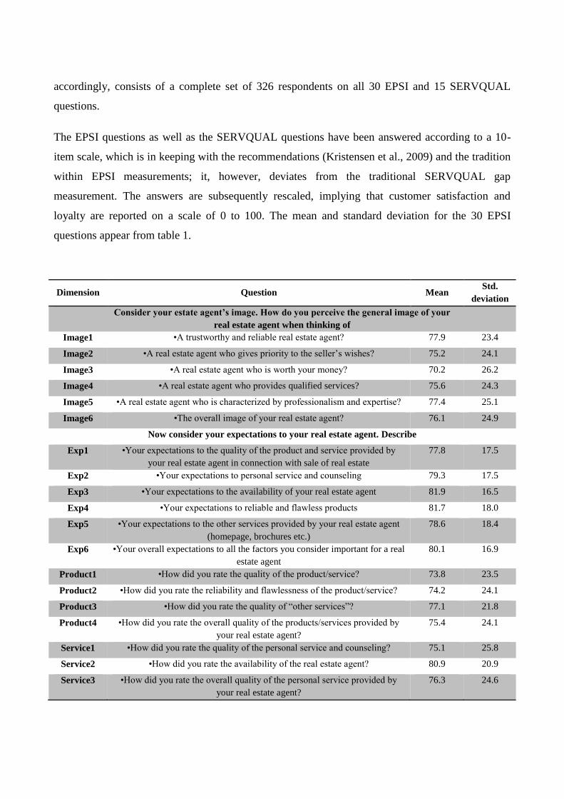
The EPSI questions as well as the SERVQUAL questions have been answered according to a 10-
item scale, which is in keeping with the recommendations (Kristensen et al., 2009) and the tradition
within EPSI measurements; it, however, deviates from the traditional SERVQUAL gap
measurement. The answers are subsequently rescaled, implying that customer satisfaction and
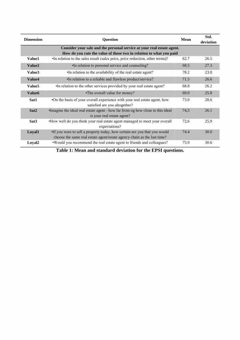
loyalty are reported on a scale of 0 to 100. The mean and standard deviation for the 30 EPSI
questions appear from table 1.
Dimension Question Mean Std.
deviation
Consider your estate agent’s image. How do you perceive the general image of your
real estate agent when thinking of
Image1 •A trustworthy and reliable real estate agent? 77.9 23.4
Image2 •A real estate agent who gives priority to the seller’s wishes? 75.2 24.1
Image3 •A real estate agent who is worth your money? 70.2 26.2
Image4 •A real estate agent who provides qualified services? 75.6 24.3
Image5 •A real estate agent who is characterized by professionalism and expertise? 77.4 25.1
Image6 •The overall image of your real estate agent? 76.1 24.9
Now consider your expectations to your real estate agent. Describe
Exp1 •Your expectations to the quality of the product and service provided by
your real estate agent in connection with sale of real estate
77.8 17.5
Exp2 •Your expectations to personal service and counseling 79.3 17.5
Exp3 •Your expectations to the availability of your real estate agent 81.9 16.5
Exp4 •Your expectations to reliable and flawless products 81.7 18.0
Exp5 •Your expectations to the other services provided by your real estate agent
(homepage, brochures etc.)
78.6 18.4
Exp6 •Your overall expectations to all the factors you consider important for a real
estate agent
80.1 16.9
Product1 •How did you rate the quality of the product/service? 73.8 23.5
Product2 •How did you rate the reliability and flawlessness of the product/service? 74.2 24.1
Product3 •How did you rate the quality of “other services”? 77.1 21.8
Product4 •How did you rate the overall quality of the products/services provided by
your real estate agent?
75.4 24.1
Service1 •How did you rate the quality of the personal service and counseling? 75.1 25.8
Service2 •How did you rate the availability of the real estate agent? 80.9 20.9
Service3 •How did you rate the overall quality of the personal service provided by
your real estate agent?
76.3 24.6
Dimension Question Mean Std.
deviation
Consider your sale and the personal service at your real estate agent.
How do you rate the value of those two in relation to what you paid
Value1 •In relation to the sales result (sales price, price reduction, other terms)? 62.7 26.5
Value2 •In relation to personal service and counseling? 68.5 27.3
Value3 •In relation to the availability of the real estate agent? 78.2 23.0
Value4 •In relation to a reliable and flawless product/service? 71.5 26.6
Value5 •In relation to the other services provided by your real estate agent? 68.8 26.2
Value6 •The overall value for money? 69.0 25.8
Sat1 •On the basis of your overall experience with your real estate agent, how
satisfied are you altogether?
73.0 28.6
Sat2 •Imagine the ideal real estate agent - how far from og how close to this ideal
is your real estate agent?
74,5
26.1
Sat3 •How well do you think your real estate agent managed to meet your overall
expectations?
72,6
25,9
Loyal1 •If you were to sell a property today, how certain are you that you would
choose the same real estate agent/estate agency chain as the last time?
74.4 30.0
Loyal2 •Would you recommend the real estate agent to friends and colleagues? 75.9 30.6
Table 1: Mean and standard deviation for the EPSI questions.

The estimation method
Common to the EPSI and EEI models is that they, like the Swedish and American customer
satisfaction indices, are estimated by means of the partial least squares (PLS) estimation technique
(Fornell et al., 1994). This method allows for estimating the relations between the latent variables,
given as a linear combination of the manifest variables, in such a way that the exogenous latent
variables are maximally correlated with the endogenous latent variables in the system.
The PLS model consists of three parts: The first part configures the internal relations that give the
connection between the latent variables:
ζΓξBηη
In this equation, η
is a vector of the latent endogenous variables with an associated coefficient
matrix, B . ξ
is a vector of the latent exogenous variables with an associated coefficient matrix,
Γ . Lastly, an error term is included, ζ
.
The other part of the model is the outer relations, which define the relation between the latent and
the manifest variables. The general equations for reflective external relations that the EPSI Rating
model is built on are:
yyεηΛy
xxεξΛx
In these equations, y
and x are vectors of the observed η
and ξ
indicators, respectively, while
yΛ
and xΛ
are the matrices that contain the iλ
coefficients combining the latent and manifest
variables. Finally, yε
and xε
designate the error terms for y
and x , respectively.
The last part of the PLS model is the weight relations: The latent variables η
and ξ
are estimated
in these relations with η̂
and ξ̂
as linear sums of the empirical indicators:
yωηη
ˆ
xωξξ
ˆ
Statistically, a covariance-based method such as LISREL can also be used to estimate the
correlation between the variables, and the literature is indeed filled with comparisons between the
two approaches (in this context, the most interesting is Tenenhaus et al. (2001)).
However, it has emerged (Jöreskog et al., 1982) that PLS is better at predicting customer and
employee loyalty than explaining it – here, LISREL has the upper hand. Furthermore, PLS is more
robust than other SEM techniques to violations of assumptions often associated with the data
generated in EPSI models – violations of assumptions such as skewed distribution of the manifest
variables, multicollinearity as well as misspecifications of the inner and outer structure (Cassel et
al., 1999; Kristensen et al., 2005; Tenenhaus, 2007; Westlund et al., 2008). As a matter of fact, the
literature refers to PLS as a distribution-free method (Vilares et al., 2009).
Finally, LISREL suffers from the limitation that the case-specific values for the latent variables in
the weight relations mentioned above cannot be determined without factor indeterminacy, making it
difficult to interpret them (Bollen, 1989). This is not the case with PLS estimation.
Empirical results
The unstandardized inner path coefficients appear from figure 2 below. As can be seen, all
coefficients are significant at least at the 5% level.

Figure 2: The estimated EPSI Rating model for the real estate business
*: significant 0.05, **: significant 0.01
As a measure of the unidimensionality, the Cronbach’s alphas (measure of internal consistency)
range from 0.934 to 0.982 and Dillon-Goldstein’s rho (better known as composite reliability) ranges
from 0.958 to 0.985. Both measures are recommended to be above 0.7, which is satisfied in this
case. In the outer model, the communalities, which measure the extent to which the variance of an
indicator is reproducible from its latent variables, should be above 0.5. The lowest communality is
0.757, implying that all indicators are kept in the model.
Finally, all indicator variables seem to point in the right direction, as all indicators correlate higher
with the latent variable they reflect than with all other latent variables.
The quality of the pure EPSI working model appears from table 2:
Measure EPSI
GoF 0.85
R2 – value 0.79
R2 – satisfaction 0.85
R2 – loyalty 0.84
RMSEA 0.04
Table 2: Statistical properties of the inner model
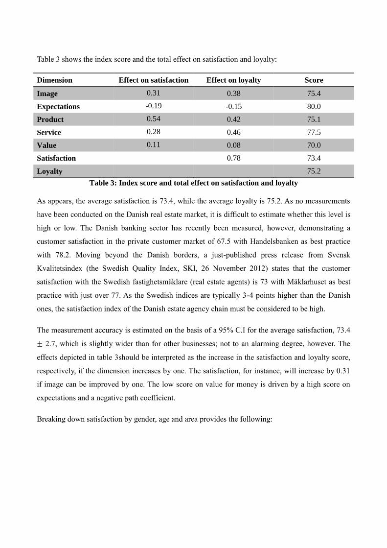
Table 3 shows the index score and the total effect on satisfaction and loyalty:
Dimension Effect on satisfaction Effect on loyalty Score
Image 0.31 0.38 75.4
Expectations -0.19 -0.15 80.0
Product 0.54 0.42 75.1
Service 0.28 0.46 77.5
Value 0.11 0.08 70.0
Satisfaction 0.78 73.4
Loyalty 75.2
Table 3: Index score and total effect on satisfaction and loyalty
As appears, the average satisfaction is 73.4, while the average loyalty is 75.2. As no measurements
have been conducted on the Danish real estate market, it is difficult to estimate whether this level is
high or low. The Danish banking sector has recently been measured, however, demonstrating a
customer satisfaction in the private customer market of 67.5 with Handelsbanken as best practice
with 78.2. Moving beyond the Danish borders, a just-published press release from Svensk
Kvalitetsindex (the Swedish Quality Index, SKI, 26 November 2012) states that the customer
satisfaction with the Swedish fastighetsmäklare (real estate agents) is 73 with Mäklarhuset as best
practice with just over 77. As the Swedish indices are typically 3-4 points higher than the Danish
ones, the satisfaction index of the Danish estate agency chain must be considered to be high.
The measurement accuracy is estimated on the basis of a 95% C.I for the average satisfaction, 73.4
± 2.7, which is slightly wider than for other businesses; not to an alarming degree, however. The
effects depicted in table 3should be interpreted as the increase in the satisfaction and loyalty score,
respectively, if the dimension increases by one. The satisfaction, for instance, will increase by 0.31
if image can be improved by one. The low score on value for money is driven by a high score on
expectations and a negative path coefficient.
Breaking down satisfaction by gender, age and area provides the following:
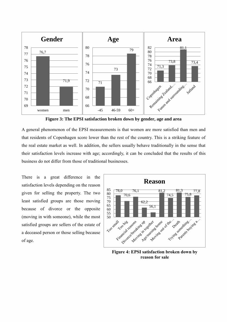
Figure 3: The EPSI satisfaction broken down by gender, age and area
A general phenomenon of the EPSI measurements is that women are more satisfied than men and
that residents of Copenhagen score lower than the rest of the country. This is a striking feature of
the real estate market as well. In addition, the sellers usually behave traditionally in the sense that
their satisfaction levels increase with age; accordingly, it can be concluded that the results of this
business do not differ from those of traditional businesses.
There is a great difference in the
satisfaction levels depending on the reason
given for selling the property. The two
least satisfied groups are those moving
because of divorce or the opposite
(moving in with someone), while the most
satisfied groups are sellers of the estate of
a deceased person or those selling because
of age.
76,7
71,9
69
70
71
72
73
74
75
76
77
78
women men
Gender
71
73
79
66
68
70
72
74
76
78
80
-45 46-59 60+
Age
71,3
73,8
81,1
73,4
666870727476788082
Area
Figure 4: EPSI satisfaction broken down by
reason for sale
78,0
70,6 76,1
62,2
56,1
81,2 74,5
81,3 75,8
77,8
5055606570758085
Reason
77,9
74,4
68,6
62
64
66
68
70
72
74
76
78
80
<=0.05 0.05-0.109 0.109+
Reduction
77,6 77,2
66,1
60
62
64
66
68
70
72
74
76
78
80
<= -2.25 0.75+
Gap in actual and
predicted selling time
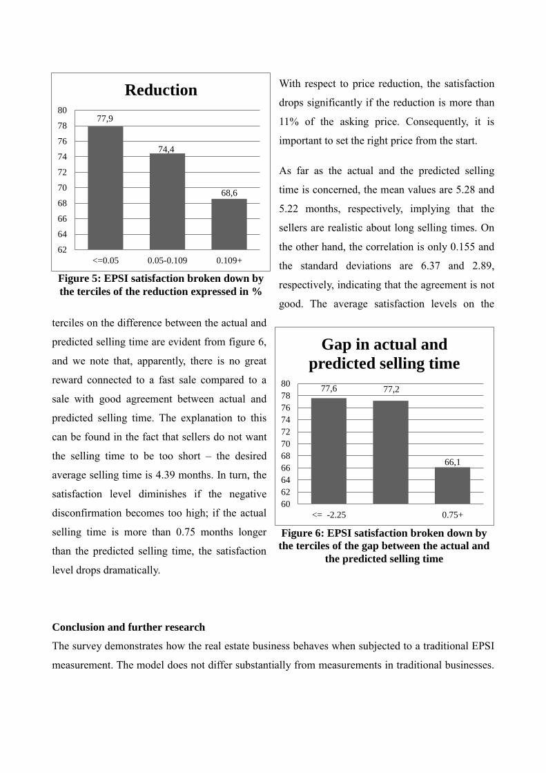
With respect to price reduction, the satisfaction
drops significantly if the reduction is more than
11% of the asking price. Consequently, it is
important to set the right price from the start.
As far as the actual and the predicted selling
time is concerned, the mean values are 5.28 and
5.22 months, respectively, implying that the
sellers are realistic about long selling times. On
the other hand, the correlation is only 0.155 and
the standard deviations are 6.37 and 2.89,
respectively, indicating that the agreement is not
good. The average satisfaction levels on the
terciles on the difference between the actual and
predicted selling time are evident from figure 6,
and we note that, apparently, there is no great
reward connected to a fast sale compared to a
sale with good agreement between actual and
predicted selling time. The explanation to this
can be found in the fact that sellers do not want
the selling time to be too short – the desired
average selling time is 4.39 months. In turn, the
satisfaction level diminishes if the negative
disconfirmation becomes too high; if the actual
selling time is more than 0.75 months longer
than the predicted selling time, the satisfaction
level drops dramatically.
Conclusion and further research
The survey demonstrates how the real estate business behaves when subjected to a traditional EPSI
measurement. The model does not differ substantially from measurements in traditional businesses.
Figure 5: EPSI satisfaction broken down by
the terciles of the reduction expressed in %
Figure 6: EPSI satisfaction broken down by
the terciles of the gap between the actual and
the predicted selling time
The path coefficients all exhibited the expected signs, and the survey has managed to create a
reliable and valid benchmark for the Danish real estate business.
The business can be accepted in Dansk KundeIndex on the same terms as other businesses if at least
60% of the turnover in the business is represented by specific companies. In order for the safety
margin with regard to the EPSI measurement of customer loyalty to be sufficiently small, at least
250 customers within each estate agency chain must be interviewed. Such a sample size will
typically result in half of the width of a 95% confidence interval for the customer satisfaction being
maximum 2. Furthermore, for the model to be accepted, at least 65% of the variation in the
customer satisfaction must be explainable. As the estate agency chain studied in this article had a
R2-satisfaction of as much as 85%, that should not pose a problem.
In a future study, the latent service dimension of the EPSI model will be supplemented /replaced by
the five SERVQUAL dimensions of reliability, responsiveness, assurance, empathy and tangibles.
The results are compared/supplemented by the service dimension from Dabholkar & Overby (2006)
in the hope of finding a robust interpretation of the service dimension that simultaneously allows for
a wider benchmarking to other companies within the knowledge service business.
Contrary to previously EPSI-studied businesses, the real estate business stands out since it operates
with two types of “customers”; the seller who pays for the service and the buyer who, strictly
speaking, receives the service for free. These customers have a common interest in concluding a
deal, but they have conflicting interests when it comes to price and terms. Even though the real
estate agent, as a rule, is the seller’s agent, he must also take measures to satisfy the buyer, thus
ensuring that he is in commission to resell the property in the future. Accordingly, the forthcoming
study will concern itself with expanding the EPSI model in order for it to handle this duality, and it
will subsequently uncover if and, if so, how the real estate agent can secure a simultaneous high
satisfaction level among both the buyer and the seller to a greater extent than now.
References
Bernhardt, K.L., Donthu, N., & Kennett, P.A.,2000: A longitudinal analysis of satisfaction and
profitability, Journal of Business Research, 47(2), 161-171.
Bollen, K.A., 1989: “Structural equations with latent variables”. New York: John Wiley & Sons
Inc.
Brown, R.L., 1994: Efficiacy of the indirect approach for estimating structural equation models
with missing data: A comparison of five methods. Structural Equation Modeling, 1, 287-316.
Cassel, C., Hackl, P., & Westlund, A.H., 1999: “Robustness of partial least-squares method for
estimating latent variables quality structures, Journal of Applied Statistics, 26(2), pp. 435-446.
Dabholkar, P.A. and Overby, J.W. (2006): An Investigation of Real Estate Agent Service to Home
Sellers: Relevant Factors and Attributions, The Service Industries Journal, Vol. 26, No. 5, July
2006, pp. 557-579.
Duboff, R., Heaton, C., 1999: Employee loyalty a link to valuable growth, Strategy & Leadership,
27(1), pp. 8-13.
Edvardsson, B., Johnson, M.D., Gustafsson, A., & Strandvik, T., 2000: The effect of satisfaction
and loyalty on profits and growth: Product versus services, Total Quality Management, 11(7), pp.
917-927.
Eklöf, J. A., Hackl, P., Westlund, A., 1999: On measuring interactions between customer
satisfaction and financial results. Total Quality Management 10 (4&5), S512-522.
ESCI Technical Committee. European Consumer Satisfaction Index: Foundation and structure for
harmonized national pilot projects. Report. October 1998.
Eskildsen, J.K., Kristensen, 2008: “Customer satisfaction and customer loyalty as predictors of
future business potential”, Total Quality Management, 19(7-8), 2008, pp. 843-853.
Fornell, C. 1992: A National Customer Satisfaction Barometer: The Swedish Experience, Journal of
Marketing, Vol. 56 (January), pp. 6-21, 1992.
Fornell, C., 1999. Customer satisfaction and shareholder value. Presented at the Fourth World
Congress for Total Quality Management, Sheffield, UK, 28-30 June 1999.
Fornell, C., Cha, J. 1994. Partial Least Squares. In ”Bagozzi, R.P.(Ed.), Advanced Methods of
Marketing Research. Blackwell, Cambridge, MA, pp. 52-78.
Juhl, H.J. et al, 2002. Customer satisfaction in European food retailing, Journal of Retailing and
Consumer Services 9 (2002) 327-334.
Jöreskog, K.G., & Wold, H., 1982: “The ML and PLS techniques for modeling with latent
variables”. In K.G. Jöreskog & H.Wold (Eds.), Systems under direct observations (pp.263-270),
New York: North Holland, 1982.
Kristensen, Kai, Martensen, A. & Grønholdt, L., 2000: Customer satisfaction measurement at Post
Denmark: Results of application of the European Customer Satisfaction Index Methodology”, Total
Quality Management, vol 11, pp. 1007-1015, 2000.
Kristensen, Kai, Martensen, A. & Grønholdt, L., 2002: ”Customer satisfaction and business
performance” I a. Neely(Ed): Business Performance Measurement – Theory and Practice, pp. 279-
294 (Cambridge: Canbridge University Press).
Kristensen, K. & Westlund, A.H., 2003: Valid and reliable measurements for suitable non-financial
reporting, Total Quality Management, Vol 14, No 2, pp. 161-170.
Kristensen, K., Eskildsen, J., 2005: “PLS structural equation modeling for customer satisfaction
measurement: Some empirical and theoretical results”. In F.W.Bliemel, A.Eggert, G.Fassott, &
J.Henseler(Eds), Handbuch PLS-Pfadmodellierung-Methode, Praxisbeispiele, pp. 117-134,
Schäffer-Poeschel.
Kristensen, K., Eskildsen, J., 2009: “Design of PLS-satisfaction studies, In Handbook of Partial
Least Squares: Concepts, Methods and Applications in Marketing and Relates fields, Springer
Handbooks of Computational Statistics, eds. V.E.Vinzi, W.W.Chin, J.Henseler and H.Wang:
Springer Verlag.
Rucci, A.J., Kirn, S. P., & Quinn, R.T.,1998: The employee-customer-profit chain at Sears, Harvard
Business Review, 76(1), pp. 83-97.

SKI: http://www.epsi-denmark.org/images/stories/Banking/epsi_bank_dk_2012_presse-final.pdf.
Olinaky, A., Chen, S.& Harlow, L., 2000, The comparative efficiacy of response categories in
rating scales: reliability, validity, discriminating power, and respondent preferences, Acta
Pstchologica, 104, 1-15.
Tenenhaus, Michel, 2007: A bridge between PLS path modeling and ULS-SEM, i “In honour of
Professor Kai Kristensen, ledelse og økonomi, 2007.
Tenenhaus, M.; Gonzales, P.L. (2001): Comparaison entre les approaches PLS et LISREL en
modelisation d’équations structurelles: Application à la mesure de la satisfaction clientele, in Actes
de 8ème Congrès de la Société Francophone de Classification Guadeloupe.
Vilares,J.M; Almeida,M.H. & Coelho,P.S.: Comparison of Likelihood and PLS Estimators for
Structural Equations Modeling: A Simulation with Customer Satisfaction Data, In Handbook of
Partial Least Squares: Concepts, Methods and Applications in Marketing and Relates fields,
Springer Handbooks of Computational Statistics, eds. V.E.Vinzi, W.W.Chin, J.Henseler and
H.Wang: Springer Verlag.
Westlund, A.H., Källström,M., Parmler,J., 2008: SEM-based customer satisfaction measurement:
On multicollinearity and robust PLS estimation. Total Quality Management, Vol. 19, Nos.7-8,
2008, pp. 855-869.
The Integration of SERVQUAL into a Customer
Satisfaction Index
– A Case Study from the Danish Real Estate Business
John Vestergaard Olesen
ICOA, BTECH, Aarhus University,
Birk Centerpark 15, 7400 Herning
Abstract
This study examines the interplay between the SERVQUAL model and a national customer
satisfaction index. The data have been obtained from a questionnaire survey conducted among
individuals who all, within a period of six months in 2012, have sold real estate in Denmark through
a real estate agent. The findings indicate that the five classic SERVQUAL dimensions can be
integrated into a national customer satisfaction index, that the framework will benefit from the
inclusion of the SERVQUAL dimensions, and that this inclusion in no way will affect traceability.
The last decade’s increasing focus on customer satisfaction and customer satisfaction measurement
is ascribable to the results of a series of empirical studies within a wide range of industries – results
that all demonstrate a close correlation between, on the one hand, customer satisfaction and
customer loyalty and, on the other, the company’s profit performance (Rucci et al., 1998;
Edvardsson et al., 2000; Eklöf et al., 1999; Fornell, 1999; Bernhardt et al., 2000; Juhl et al., 2002;
Kristensen et al., 2002; Eskildsen et al., 2008). The company’s value can thus be seen as a function

of its assets, and seeing that intangible assets constitute an increasingly greater part of this value, the
level of customer satisfaction could be considered a good indicator of the company’s future earning
capacity.
A tool for making these customer satisfaction measurements is the so-called EPSI (European
Satisfaction Performance Measurement) model, in which the three dimensions of value for money,
satisfaction, and loyalty are determined by the four dimensions of image, expectations, and product
and service quality. We have come to know quite a bit about the model and its structure in a wide
range of industries, and valid and reliable industry benchmarks have been created.
One of the great advantages of national customer satisfaction models is that they, using a series of
suitably flexible, yet generic questions, can be employed in a vast array of different industries. This
advantage, however, is also the weakness of the models, as the companies are often left with a
number of indices, which are useful for benchmarking against other countries, companies,
industries, and organizations, but are limited in providing knowledge about how to improve, for
instance, the quality of service. In spite of this, little effort has been made to integrate established
measurement systems such as SERVQUAL into a national customer satisfaction framework – and
that is exactly the focus of this study.
If the integration goes well, the hope is to take the best from both worlds and end up with a model
that is able to both provide deeper insights into the interpretation of the EPSI index and, by means
of the SERVQUAL dimensions, provide us with useful information on how to improve the service
quality.
National customer satisfaction indices
In 1989, Sweden became the first country to establish a standardized method for measuring
customer satisfaction and customer loyalty across companies and industries. Originally dubbed the
Swedish Customer Satisfaction Barometer (SCSB), it built on the Swedish-born professor Claes
Fornell’s customer satisfaction model (Fornell, 1992). Fornell continued his work on the model at
the National Quality Center (NQRC) at the University of Michigan, and, in 1994, he constructed an
American sister index, the American Customer Satisfaction Index (ASCI). The successful
application of these indices led the European Commission to decide in 1998 that Europe needed an
equivalent standardized measurement instrument for customer satisfaction.
The result of the subsequent work performed by the European Consumer Satisfaction Index
Technical Committee (ESCI, 1998) was first known as ECSI (the European Customer Satisfaction
Index), then changed its name to the EPSI Rating model (the European Performance Satisfaction
Index/Extended Performance Satisfaction Index). Since then, the model has produced results that
are comparable with figures from the participating countries within a variety of industries.
In Europe, EPSI Rating is managed by the European Foundation for Quality Management (EFQM),
which is also behind the European Quality Award, the European Organization for Quality (EOQ),
and the International Foundation for Customer Focus (IFCF) (research network) (Kristensen &
Westlund, 2003).
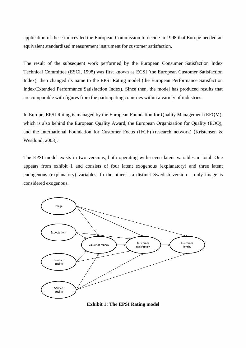
The EPSI model exists in two versions, both operating with seven latent variables in total. One
appears from exhibit 1 and consists of four latent exogenous (explanatory) and three latent
endogenous (explanatory) variables. In the other – a distinct Swedish version – only image is
considered exogenous.
Exhibit 1: The EPSI Rating model

Behind all seven latent dimensions lie a number of measurable (manifest) variables, which are
explored. Naturally, in practice, many other connections than those indicated by the arrows may be
included in the model, as it only depicts the expected connections (Kristensen et al., 2000).
The ASCI model as well as the two versions of the EPSI model are structural equation models,
composed partly of a structural part, which gives the relations between the latent variables, partly of
a measurement part, which gives the relations between the manifest and latent variables, and partly
weight relations. A common feature of all the models is that loyalty is the ultimate expression of
customer satisfaction and, accordingly, what ultimately needs to be explained. The ASCI model
differs from the two EPSI models by having only six latent variables, only one exogenous variable
(expectations), by merging product and service quality into one dimension (perceived quality), and,
finally, by not incorporating image, but instead having a dimension called “customer complaints”.
Studies have shown that the index estimates remain the same no matter which EPSI model is
employed (Kristensen et al., 2009), and as the same is expected in relation to the ASCI model, this
study continues to work with the EPSI model due to the fact that instead of merging the service
dimension and the product dimension, it has preserved the division.
The concept of service/SERVQUAL
Many attempts have been made to develop service quality models, and a review (Seth et al., 2005)
has managed to identify as much as 19 models. The general study of the service quality dimension
began to take definite shape in the mid-eighties, when Zeithaml, Parasuraman, and Berry
conceptualized and operationalized the service quality construct and thus developed the so-called
SERVQUAL (SERVice QUALity) instrument (Parasuraman et al., 1985, 1988).
SERVQUAL should be understood as a tool framework consisting of five sub-dimensions – so-
called factors – which were originally operationalized as 22 double questions. The five factors are:
Reliability (ability to deliver the promised service)
Responsiveness (willingness to provide prompt service)
Assurance (ability to inspire trust and confidence)
Empathy (caring about the customer)

Tangibles (facilities and appearance of personnel)
In the original version (Parasuraman et al., 1985, 1988), each factor is measured by 4-5 double
items, the idea behind the SERVQUAL instrument being that the respondents indicate on a 7-item
Likert scale (1=”strongly disagree” to 7=”strongly agree”) the degree to which they agree with
statements concerning their service expectations and their perception of the delivered service.
The gap score is then, on an item-by-item basis, defined as the difference between the service
performance and the service expectation
gap score = service performance – service expectation
and is, accordingly, a figure between -6 and +6. The higher the gap score, the higher is the
perceived service quality (Parasuraman et al., 1988).
The original development of the SERVQUAL model was based on research within very different
industries, for instance, retail banking, repair and maintenance and electrical appliances, credit card
services, title brokerage, and long-distance telephone services. The model has since, by means of
different methods (CFA, EFA, SEM), demonstrated adequate fit and stability in a wide range of
B2C relationships within sectors such as the banking industry (Cronin et al., 1992; Mels et al.,
1997; Duffy et al., 1997; Parasuraman et al., 1991; Lam, 2002; Zhou, 2002; Chi Cui et al., 2003;
Arasli et al., 2005), the health sector (Carman, 1990; Headley et al., 1993; Lam, 1997; Kilbourne et
al., 2004), the educational sector (Kettinger et al., 1994; Engelland et al., 2000; Kang et al., 2002),
the insurance business (Parasuraman et al., 1991; Mels et al., 1997; Baldwin et al., 2003), the
library world (Nitecki, 1996; Cook et al., 2000), and the B2B world (Gounaris, 2005). In terms of
geography, the above-mentioned studies have included countries such as the USA, the UK,
Australia, South Africa, Cyprus, China, Hong Kong, Korea, and Holland.
At the same time, in the realization that a number of industry-specific circumstances may exist that
necessitate customizing the model to the individual industry (Carman, 1990; Vandamme et al.,
1993), Ladhari (2008) identifies as much as 30 industry-specific adjustments to the SERVQUAL
scale with items ranging between 14 (Shemwell et al., 1999) and 75 (Sower et al., 2001) and factors
ranging between 2 (Ekinci et al., 1998) and 10 (Vaughan et al.,2001).

As is evident from the numerous studies of industry-tailored models, the five dimensions of the
SERVQUAL model have, in the last 20 years, been criticized for not being generic and universal.
Additionally, the model has been met with criticism concerning, among other things:
Reliability (Peter et al., 1993; Duffy et al., 1997; van der Wal et al., 2002; Badri et al.,
2005).
Convergent validity (Carman, 1990; Parasuraman et al., 1991; Mels et al., 1997; Engelland
et al., 2000; Lam, 2002).
Discriminant validity (Carman, 1990; Babakus et al., 1992; Cook et al., 2000; Kilbourne et
al., 2004).
Predictive validity (Brown et al., 1993; Durvasula et al., 1999; Zhou et al., 2002; Brady et
al., 2002).
The gap score concept, which does not have any equivalent in or build on established
economic, psychological, and statistical theory (Cronin et al., 1992; Peter et al., 1993;
Brown et al., 1993; Ekinci et al., 1998).
Despite the theoretical and empirical criticism leveled against it, the SERVQUAL model has
managed to establish itself as a recognized, generic method for measuring service quality. When
applied to the real estate business, the SERVQUAL model could be operationalized as indicated in
exhibit 2.
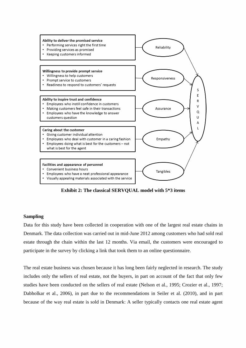
Exhibit 2: The classical SERVQUAL model with 5*3 items
Sampling
Data for this study have been collected in cooperation with one of the largest real estate chains in
Denmark. The data collection was carried out in mid-June 2012 among customers who had sold real
estate through the chain within the last 12 months. Via email, the customers were encouraged to
participate in the survey by clicking a link that took them to an online questionnaire.
The real estate business was chosen because it has long been fairly neglected in research. The study
includes only the sellers of real estate, not the buyers, in part on account of the fact that only few
studies have been conducted on the sellers of real estate (Nelson et al., 1995; Crozier et al., 1997;
Dabholkar et al., 2006), in part due to the recommendations in Seiler et al. (2010), and in part
because of the way real estate is sold in Denmark: A seller typically contacts one real estate agent

who is commissioned to sell the property. Potential buyers are then to contact this agent directly in
order to see and possibly buy the property. Accordingly, only one real estate agent is on
commission to sell the property, and only the seller pays for the service of the real estate agent – for
the buyer, the service is free. Even though the real estate agent, as a rule, is the seller’s agent, he
must also take measures to satisfy the buyer to ensure that he is in commission to resell the property
in the future. It has been suggested (Seiler et al., 2008) that buyers are more interesting than sellers,
as they could be leaving the area, whereas the buyers are certainly part of the estate agent’s
geographical scope. True as that may be, part of the sellers remain in the area and thus have the
opportunity to use the same real estate agent when “reselling” their house. In addition, most real
estate agents in Denmark are organized in real estate chains, so even if the sellers move away from
the area, a high level of satisfaction will, if nothing else, lead to a sense of loyalty towards the
chain. Finally, in all probability, the seller will share his experiences and level of estate agent
satisfaction with his former neighbors and additional social network connections in his old
neighborhood.
The questionnaire consisted of 30 questions, together covering the EPSI part, as well as the 15
questions indicated in exhibit 2, which covered the five SERVQUAL dimensions (with three
questions addressing each dimension). Only items related to perception are included in accordance
with findings in Cronin et al., (1992), Brown et al. (1993), McAlexander et al. (1994), and
Durvasula et al. (1999).
The email was sent to 2,800 customers, 442 of whom clicked the survey link. This corresponds to
just fewer than 16%. Of the 442 respondents, 326 had answered all 30 EPSI questions, but a few
had failed to answer all 15 SERVQUAL questions. Seeing that the EM and regression substitution
(Brown, 1994; Olinsky et al., 2003) are preferred to pairwise deletion and mean substitution in
general, and in customer satisfaction analyses, as in a PLS model, in particular (Kristensen et al.,
2009), and seeing that the inclination is to prefer the EM substitution to the regression-based
substitution, the EM algorithm is used to fill the few holes in the dataset, which, accordingly,
consists of a complete set of 326 respondents on all 30 EPSI and 15 SERVQUAL questions.
All the EPSI questions as well as the SERVQUAL questions have been answered according to a 10-
item scale, which is in keeping with the recommendations (Kristensen et al., 2009) and the tradition

within the EPSI measurements; it, however, deviates from the traditional SERVQUAL gap
measurement (Parasuraman et al., 1988).
The estimation method
Common to the EPSI and EEI models is that they, like the Swedish and American customer
satisfaction indices, are estimated by means of the partial least squares (PLS) estimation technique
(Fornell et al., 1994). This method allows for estimating the relations between the latent variables,
given as a linear combination of the manifest variables, in such a way that the exogenous latent
variables are maximally correlated with the endogenous latent variables in the system.
The PLS model consists of three parts: The first part is the structural model, in which we have the
internal relations between the latent variables:
ζΓξBηη
In this equation, η
is a vector of the latent endogenous variables with an associated coefficient
matrix, B . ξ
is a vector of the latent exogenous variables with an associated coefficient matrix,
Γ . Lastly, a residual vector is included, ζ
.
The other part of the model is the measurement model or the outer part, which defines the relation
between the latent and the manifest variables. The general equations for the reflective external
relations that the EPSI Rating model is built on are:
yyεηΛy
xxεξΛx

In these equations, y
and x are vectors of the observed η
and ξ
indicators, respectively, while
yΛ
and xΛ
are the matrices that contain the iλ
coefficients combining the latent and manifest
variables. Finally, yε
and xε
designate the error vectors for y
and x , respectively.
The last part of the PLS model is the weight relations: The latent variables η
and ξ
are estimated
in these relations with η̂
and ξ̂
as linear sums of the empirical indicators:
yωηη
ˆ
xωξξ
ˆ
Statistically, a covariance-based method such as LISREL can also be used to estimate the
correlation between the variables, and the literature is indeed filled with comparisons between the
two approaches (in this context, the most interesting is Tenenhaus et al. (2001)); however, the
literature has also shown (Jöreskog et al., 1982) that PLS is better at predicting customer and
employee loyalty than explaining it – here, LISREL has the upper hand. Furthermore, PLS is less
sensitive than other SEM techniques to violations of assumptions, such as skewed distribution,
multicollinearity as well as misspecifications of the model (Cassel et al., 1999; Kristensen et al.,
2005; Tenenhaus, 2007; Westlund et al., 2008).
Finally, LISREL suffers from the limitation that the case-specific values for the latent variables in
the weight relations mentioned above cannot be determined without factor indeterminacy, making it
difficult to interpret them (Bollen, 1989). This is not the case with PLS estimation.
Empirical results
The pure EPSI model is estimated with value, satisfaction, and loyalty as latent endogenous
dimensions and image, expectations, product, and service as latent exogenous dimensions. The
unstandardized inner coefficients and the dimension scores appear from exhibit 3:
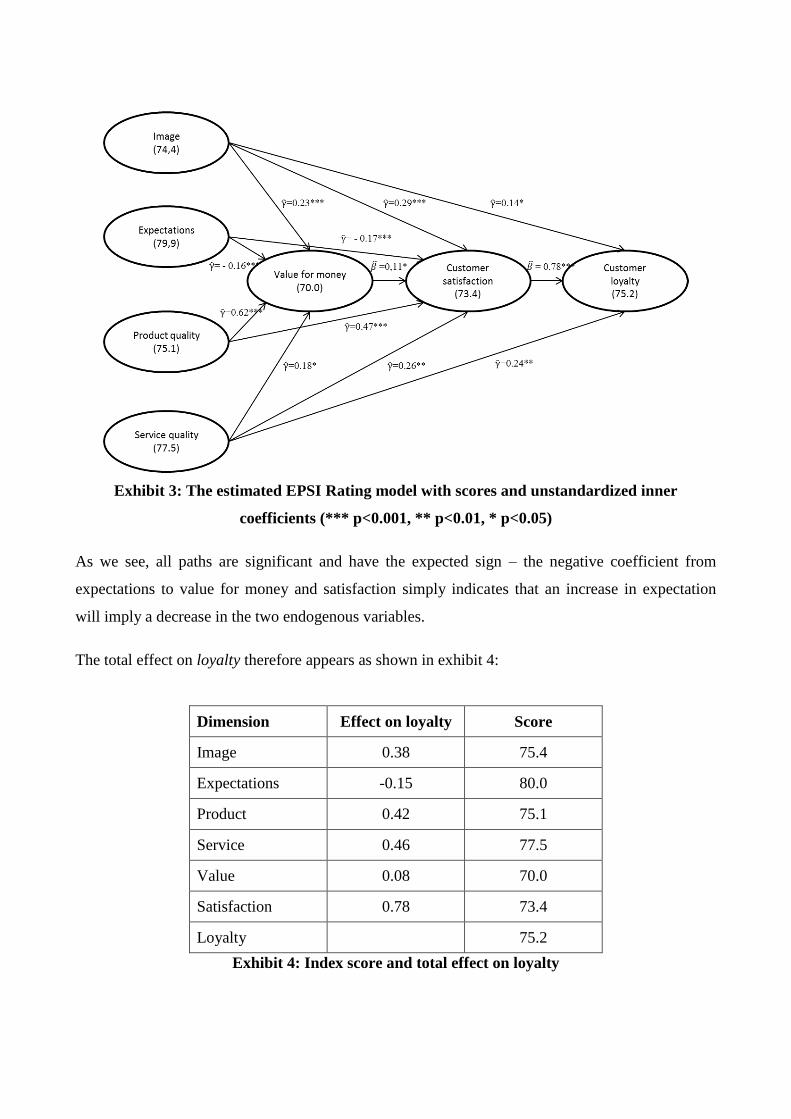
Exhibit 3: The estimated EPSI Rating model with scores and unstandardized inner
coefficients (*** p<0.001, ** p<0.01, * p<0.05)
As we see, all paths are significant and have the expected sign – the negative coefficient from
expectations to value for money and satisfaction simply indicates that an increase in expectation
will imply a decrease in the two endogenous variables.
The total effect on loyalty therefore appears as shown in exhibit 4:
Dimension Effect on loyalty Score
Image 0.38 75.4
Expectations -0.15 80.0
Product 0.42 75.1
Service 0.46 77.5
Value 0.08 70.0
Satisfaction 0.78 73.4
Loyalty 75.2
Exhibit 4: Index score and total effect on loyalty

As a measure of the unidimensionality, the Cronbach’s alphas (measure of internal consistency)
range from 0.934 to 0.982 and Dillon-Goldstein’s rho (better known as composite reliability) ranges
from 0.958 to 0.985. Both measures are recommended to be above 0.7. In the outer model, the
communalities, which measure the extent to which the variance of an indicator is reproducible from
its latent variables, should be above 0.5, thus providing information rather than noise. The lowest
communality is 0.757, implying that all indicators are kept in the model.
Finally, all indicators seem to point in the correct directions, as they all correlate higher with the
latent variable they reflect than with all other latent variables.
The overall measure of prediction performance of the model is computed by the global criterion of
goodness of fit proposed by Tenenhaus et al. (2004). The index is a measure that takes into account
the model performance in both the measurement model and the structural model, and it is computed
as the geometrical average of the average R2 values from the structural model and the weighted
average communality index, where the number of manifest variables of each construct are used as
weight:
GoFabsolute = √Communality̅̅ ̅̅ ̅̅ ̅̅ ̅̅ ̅̅ ̅̅ ̅̅ ̅ ∙ R2̅̅ ̅
If each index in the computation of this absolute measure is related to its maximum value, we get
the relative GoF measure. Both measures are descriptive, and there are no thresholds by which to
judge the statistical significance of their values. However, they are both bounded between 0 and 1,
and an absolute GoF above 0.7 and a relative GoF of at least 0.90 are said to speak in favor of the
model (Vinzi et al., 2010). In the present situation, the measures are 0.85 and 0.98, respectively.
The quality of the EPSI model appears from exhibit 5:
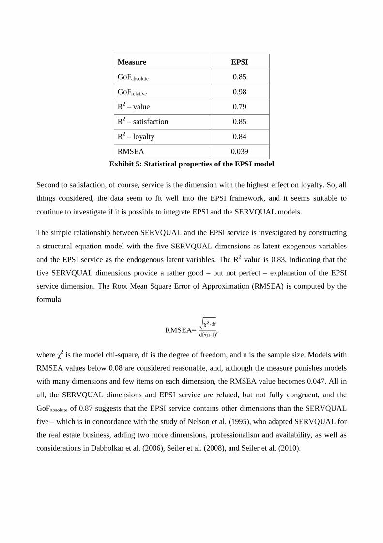
Measure EPSI
GoFabsolute 0.85
GoFrelative 0.98
R2 – value 0.79
R2 – satisfaction 0.85
R2 – loyalty 0.84
RMSEA 0.039
Exhibit 5: Statistical properties of the EPSI model
Second to satisfaction, of course, service is the dimension with the highest effect on loyalty. So, all
things considered, the data seem to fit well into the EPSI framework, and it seems suitable to
continue to investigate if it is possible to integrate EPSI and the SERVQUAL models.
The simple relationship between SERVQUAL and the EPSI service is investigated by constructing
a structural equation model with the five SERVQUAL dimensions as latent exogenous variables
and the EPSI service as the endogenous latent variables. The R2 value is 0.83, indicating that the
five SERVQUAL dimensions provide a rather good – but not perfect – explanation of the EPSI
service dimension. The Root Mean Square Error of Approximation (RMSEA) is computed by the
formula
RMSEA= √χ2-df
df∙(n-1),
where χ2 is the model chi-square, df is the degree of freedom, and n is the sample size. Models with
RMSEA values below 0.08 are considered reasonable, and, although the measure punishes models
with many dimensions and few items on each dimension, the RMSEA value becomes 0.047. All in
all, the SERVQUAL dimensions and EPSI service are related, but not fully congruent, and the
GoFabsolute of 0.87 suggests that the EPSI service contains other dimensions than the SERVQUAL
five – which is in concordance with the study of Nelson et al. (1995), who adapted SERVQUAL for
the real estate business, adding two more dimensions, professionalism and availability, as well as
considerations in Dabholkar et al. (2006), Seiler et al. (2008), and Seiler et al. (2010).

Exhibit 6: The SERVQUAL dimensions as predictors of the EPSI service
(*** p<0.001, ** p<0.01, * p<0.05)
If we added the professionalism dimension (p<0.00001), the R2
and GoF would increase to 0.88 and
0.89, respectively, and the RMSEA decrease to 0.046. However, since we are interested in keeping
traceability and since the focus of this study is to see the degree to which the SERVQUAL models
can be integrated in the EPSI Rating framework, we use the traditional SERVQUAL with the five
dimensions of reliability, responsiveness, assurance, empathy, and tangibles.
The dimensions reliability, responsiveness, and empathy are all significant (p<0.005), but assurance
(p=0.44) and tangibles (p=0.31) are insignificant. Responsiveness is the most important with an
unstandardized inner coefficient of 0.40. The remaining coefficients and the mean value of the
latent variables appear from exhibit 4. These findings support the findings in Seiler et al. (2008),
who also found that reliability, responsiveness, and empathy all significantly explained an overall
service quality measure for home buyers; responsiveness being the most important, assurance being
insignificant, and tangibles being significant (with a negative effect, however). McDaniel et al.
(1994) only found reliability and assurance to be statistically significant. Especially concerning the
dimension empathy, the lowest scoring dimension, there is room for improvement, and each time
we improve the empathy score with one, we expect to improve the EPSI service with 0.21. From

exhibit 4, we remember that service was the exogenous dimension with the heaviest impact on
loyalty in the full EPSI model.
If split by the gender, we see that the SERVQUAL dimensions work differently in different
segments: As usual, women have higher scores than men (Kristensen et al., 2009, Eskildsen et al.,
2012), but for women, only responsiveness and empathy are significant; responsiveness still being
by far the most important with a coefficient of 0.68. For men, reliability and empathy are still
significant, but responsiveness has become insignificant. On the other hand, assurance has now
become significant with the second-highest impact on EPSI service. Tangibles are also unimportant
to men.
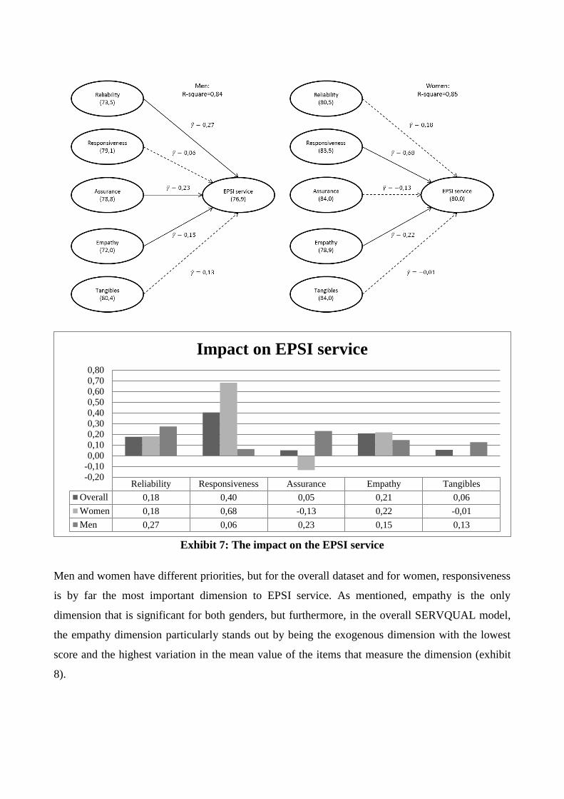
Exhibit 7: The impact on the EPSI service
Men and women have different priorities, but for the overall dataset and for women, responsiveness
is by far the most important dimension to EPSI service. As mentioned, empathy is the only
dimension that is significant for both genders, but furthermore, in the overall SERVQUAL model,
the empathy dimension particularly stands out by being the exogenous dimension with the lowest
score and the highest variation in the mean value of the items that measure the dimension (exhibit
8).
Reliability Responsiveness Assurance Empathy Tangibles
Overall 0,18 0,40 0,05 0,21 0,06
Women 0,18 0,68 -0,13 0,22 -0,01
Men 0,27 0,06 0,23 0,15 0,13
-0,20-0,100,000,100,200,300,400,500,600,700,80
Impact on EPSI service

Dimension Item Mean Variation
Reliability
Performing services right the first time 73.8
6.5 Providing services as promised 75.9
Keeping customers informed 77.4
Responsiveness
Willingness to help customers 80.8
0.7 Prompt service to customers 79.8
Readiness to respond to customers’ request 79.8
Assurance
Employees who instill confidence in customers 79.8
1.2 Making customers feel safe in their transactions (trusted that
the agent did everything correctly) 79.8
Employees who have the knowledge to answer customer
questions 81.1
Empathy
Giving customers individual attention (using my needs as a
starting point) 75.1
50.4 Employees who deal with customers in a caring fashion 78.2
My agent did what was best for me – not what was best for
the agent 68.3
Tangibles
Convenient business hours 81.0
1.1 Employees who have a neat professional appearance 81.9
Visually appealing materials associated with the service
(appealing homepage, brochure, and other information
material)
80.5
Exhibit 8: The mean score of the 15 SERVQUAL items and the variation in the scores of the
five dimensions
Looking at the empathy dimension, the item “my agent did what was best for me – not what was
best for the agent” stands out in a negative way by being the item with by far the lowest mean
value. If we use this item to split the dataset into terciles and compute the mean scores of the
endogenous variables in the pure EPSI model, we see a very strong link to the stated value,
satisfaction, and loyalty. The item is thus a very vital part of the empathy that should be a focus area
of the sector.
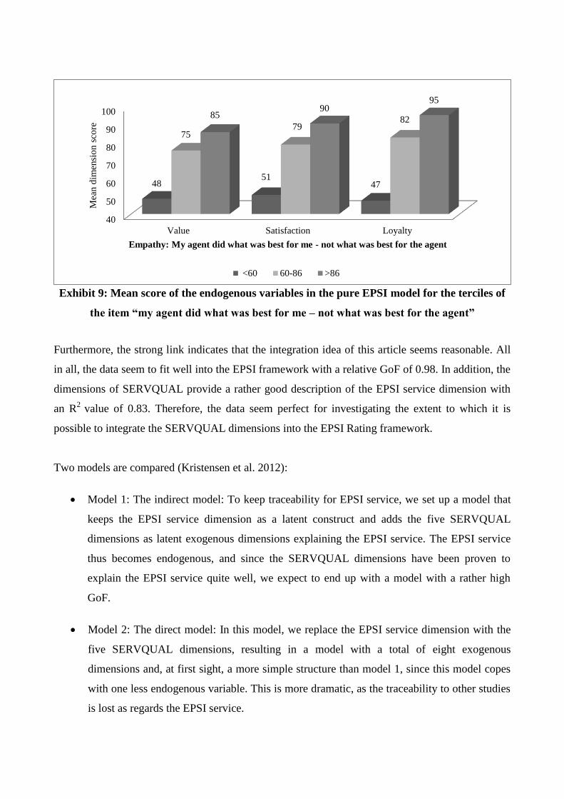
Exhibit 9: Mean score of the endogenous variables in the pure EPSI model for the terciles of
the item “my agent did what was best for me – not what was best for the agent”
Furthermore, the strong link indicates that the integration idea of this article seems reasonable. All
in all, the data seem to fit well into the EPSI framework with a relative GoF of 0.98. In addition, the
dimensions of SERVQUAL provide a rather good description of the EPSI service dimension with
an R2
value of 0.83. Therefore, the data seem perfect for investigating the extent to which it is
possible to integrate the SERVQUAL dimensions into the EPSI Rating framework.
Two models are compared (Kristensen et al. 2012):
Model 1: The indirect model: To keep traceability for EPSI service, we set up a model that
keeps the EPSI service dimension as a latent construct and adds the five SERVQUAL
dimensions as latent exogenous dimensions explaining the EPSI service. The EPSI service
thus becomes endogenous, and since the SERVQUAL dimensions have been proven to
explain the EPSI service quite well, we expect to end up with a model with a rather high
GoF.
Model 2: The direct model: In this model, we replace the EPSI service dimension with the
five SERVQUAL dimensions, resulting in a model with a total of eight exogenous
dimensions and, at first sight, a more simple structure than model 1, since this model copes
with one less endogenous variable. This is more dramatic, as the traceability to other studies
is lost as regards the EPSI service.
40
50
60
70
80
90
100
Value Satisfaction Loyalty
48 51
47
75 79
82 85
90 95
Mea
n d
imen
sio
n s
core
Empathy: My agent did what was best for me - not what was best for the agent
<60 60-86 >86

Exhibit 10: Model 1: Indirect estimation,
where the 5 SERVQUAL dimensions are
added to the EPSI model
Exhibit 11: Model 2: Direct estimation,
where the EPSI service dimension is
replaced by the 5 SERVQUAL dimensions
The fit measures for the two models and for the pure EPSI appear from exhibit 12. As can be seen,
the SERVQUAL dimensions in both models can be successfully integrated into the EPSI Rating
framework. The indirect estimation in model 1 has a slightly better GoF and higher R2
on
satisfaction and loyalty than the direct estimation in model 2, whereas model 2 is marginally better
at predicting value and has the lowest RMSE.
EPSI Model 1 Model 2
GoF 0.8530 0.8573 0.8567
R2 – value 0.7911 0.7915 0.7964
R2 – satisfaction 0.8486 0.8486 0.8469
R2 – loyalty 0.8428 0.8428 0.8420
RMSE 0.0388 0.0393 0.0379
Exhibit 12: A comparison of the statistical properties of the standard EPSI model and the
models with indirect and direct integration of the SERVQUAL dimensions
When comparing the EPSI scores with the scores from the new models, exhibit 12 shows,
consistent with Kristensen et al. (2009), that the differences are quite small – the largest difference
being 0.05 for comparable indices. Consequently, introducing the five SERVQUAL dimensions
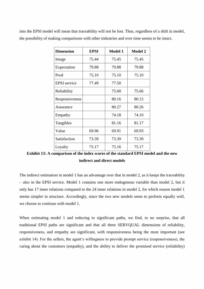
into the EPSI model will mean that traceability will not be lost. Thus, regardless of a shift in model,
the possibility of making comparisons with other industries and over time seems to be intact.
Dimension EPSI Model 1 Model 2
Image 75.44 75.45 75.45
Expectation 79.88 79.88 79.88
Prod 75.10 75.10 75.10
EPSI service 77.49 77.50
Reliability
75.68 75.66
Responsiveness
80.16 80.15
Assurance
80.27 80.26
Empathy
74.18 74.10
Tangibles
81.16 81.17
Value 69.96 69.91 69.93
Satisfaction 73.39 73.39 73.39
Loyalty 75.17 75.16 75.17
Exhibit 13: A comparison of the index scores of the standard EPSI model and the new
indirect and direct models
The indirect estimation in model 1 has an advantage over that in model 2, as it keeps the traceability
– also in the EPSI service. Model 1 contains one more endogenous variable than model 2, but it
only has 17 inner relations compared to the 24 inner relations in model 2, for which reason model 1
seems simpler in structure. Accordingly, since the two new models seem to perform equally well,
we choose to continue with model 1.
When estimating model 1 and reducing to significant paths, we find, to no surprise, that all
traditional EPSI paths are significant and that all three SERVQUAL dimensions of reliability,
responsiveness, and empathy are significant, with responsiveness being the most important (see
exhibit 14). For the sellers, the agent’s willingness to provide prompt service (responsiveness), the
caring about the customers (empathy), and the ability to deliver the promised service (reliability)
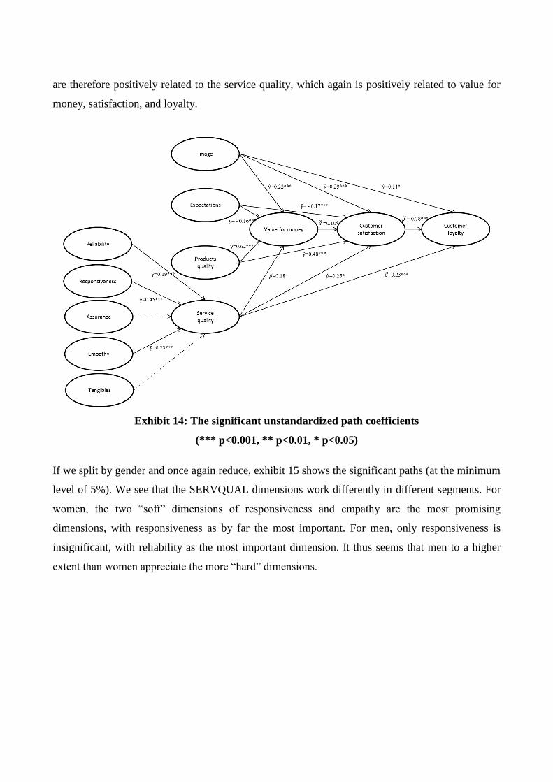
are therefore positively related to the service quality, which again is positively related to value for
money, satisfaction, and loyalty.
Exhibit 14: The significant unstandardized path coefficients
(*** p<0.001, ** p<0.01, * p<0.05)
If we split by gender and once again reduce, exhibit 15 shows the significant paths (at the minimum
level of 5%). We see that the SERVQUAL dimensions work differently in different segments. For
women, the two “soft” dimensions of responsiveness and empathy are the most promising
dimensions, with responsiveness as by far the most important. For men, only responsiveness is
insignificant, with reliability as the most important dimension. It thus seems that men to a higher
extent than women appreciate the more “hard” dimensions.

Exhibit 15: Unstandardized path coefficients for model 1, split by gender
As can be seen from exhibit 16, the two gender submodels are indeed different, and, to no surprise,
responsiveness is one of the dimensions, where the two models perform differently. Furthermore,
the paths from assurance to EPSI service and from expectations to satisfaction are different.
Women
Path coefficient T statistic Sign
Image Satisfaction 0.201 2.67 **
Expectation Value -0.170 -2.16 *
Product Value 0.931 17.26 ***
Product Satisfaction 0.429 2.81 **
Responsiveness Service 0.710 8.16 ***
Empathy Service 0.238 2.69 **
Service Satisfaction 0.395 2.91 **
Service Loyalty 0.241 2.44 *
Satisfaction Loyalty 0.845 9.06 ***
Notes: *** p<0.001, ** p<0.01, * p<0.05.
Men
Path coefficient T statistic Sign
Image Value 0.317 5.19 ***
Image Satisfaction 0.356 5.16 ***
Expectation Satisfaction -0.314 -4.82 ***
Product Value 0.690 10.12 ***
Product Satisfaction 0.633 6.63 **
Reliability Service 0.288 4.98 ***
Assurance Service 0.254 3.66 ***
Empathy Service 0.144 2.12 *
Tangibles Service 0.151 2.41 *
Service Loyalty 0.408 4.66 ***
Value Satisfaction 0.215 2.65 **
Satisfaction Loyalty 0.780 10.87 ***
Notes: *** p<0.001, ** p<0.01, * p<0.05.
Path
Path
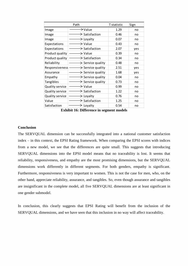
T statistic Sign
Image Value 1.29 no
Image Satisfaction 0.46 no
Image Loyalty 0.07 no
Expectations Value 0.43 no
Expectations Satisfaction 2.07 yes
Product quality Value 0.39 no
Product quality Satisfaction 0.34 no
Reliability Service quality 0.48 no
Responsiveness Service quality 2.51 yes
Assurance Service quality 1.68 yes
Empathy Service quality 0.04 no
Tangibles Service quality 0.73 no
Quality service Value 0.99 no
Quality service Satisfaction 1.22 no
Quality service Loyalty 0.76 no
Value Satisfaction 1.25 no
Satisfaction Loyalty 0.54 no
Path
Exhibit 16: Difference in segment models
Conclusion
The SERVQUAL dimension can be successfully integrated into a national customer satisfaction
index – in this context, the EPSI Rating framework. When comparing the EPSI scores with indices
from a new model, we see that the differences are quite small. This suggests that introducing
SERVQUAL dimensions into the EPSI model means that no traceability is lost. It seems that
reliability, responsiveness, and empathy are the most promising dimensions, but the SERVQUAL
dimensions work differently in different segments. For both genders, empathy is significant.
Furthermore, responsiveness is very important to women. This is not the case for men, who, on the
other hand, appreciate reliability, assurance, and tangibles. So, even though assurance and tangibles
are insignificant in the complete model, all five SERVQUAL dimensions are at least significant in
one gender submodel.
In conclusion, this clearly suggests that EPSI Rating will benefit from the inclusion of the
SERVQUAL dimensions, and we have seen that this inclusion in no way will affect traceability.
References
Arasli, H., Mehtap-Smadi, S. and Katircioglu, S.T., 2005: Customer service quality in the Greek
Cypriot banking industry, Managing Service Quality, 15: 1 pp. 41-56.
Babakus, E., Boller, G.W., 1992: An empirical assessment of the SERVQUAL scale, Journal of
Business Research, 1992, 24, 253-68.
Badri, M.A., Abdulla, M. & Al-Madani, A., 2005: Information technology center service quality:
assessment and application of SERVQUAL, International Journal of Quality & Reliability
Management, 22:8/9, pp. 819-48.
Baldwin, A. & Sohal, A. 2003: Service quality factors and outcomes in dental care, Managing
Service Quality, 13: 3, pp. 207-16.
Bernhardt, K.L., Donthu, N., & Kennett, P.A., 2000: A longitudinal analysis of satisfaction and
profitability, Journal of Business Research, 47: 2, 161-171.
Bollen, K.A., 1989: “Structural equations with latent variables”. New York: John Wiley & Sons
Inc.
Brady, M.K., Cronin, J.J. & Brand, R.R., 2002: Performance-only measurement of service quality:
a replication and extension, Journal of Business Research, 55: 1, pp. 17-31.
Brown, T. J., Churchill, G.A. & Peter, J.P., 1993: Research note: improving the measurement of
service quality, Journal of Retailing, 69: 1, pp. 127-39.
Brown, R.L., 1994: Efficacy of the indirect approach for estimating structural equation models with
missing data: A comparison of five methods. Structural Equation Modeling, 1, 287-316.
Carman, J.M., 1990: Consumer Perception of Service Quality: An assessment of the SERVQUAL
Dimensions, Journal of Retailing, Spring 1990, 66: 1, 33-55.
Cassel, C., Hackl, P., & Westlund, A.H., 1999: “Robustness of partial least-squares method for
estimating latent variables quality structures, Journal of Applied Statistics, 26(4), pp. 435-446.
Chi Cui, C., Lewis, B.R. & Park, W., 2003: Service quality measurement in the banking sector in
South Korea”, International Journal of Bank Marketing, 21(4/5).
Cook, C. & Thompson, B., 2000: Reliability and validity of SERVQUAL scores used to evaluate
perceptions of library service quality, Journal of Academic Librarianship, 26: 4, pp. 248-58.
Cronin, J. J., Taylor, S.A., 1992: Measuring Service Quality: A Reexamination and extension,
Journal of Marketing, July 1992, 56, pp. 55-68.
Crozier, D.A., McLean, F., 1997: Consumer decision-making in the purchase og estate agency
services. The Service Industries Journal, 17(2), pp. 278-293.
Dabholkar, P.A. and Overby, J.W., 2006: An Investigation of Real Estate Agent Service to Home
Sellers: Relevant Factors and Attributions, The Service Industries Journal, 26: 5, pp. 557-579.
Duffy, J.A., Duffy, M. & Kilbourne, W., 1997: Cross national study of perceived service quality in
long-term care facilities, Journal of Aging Studies 11: 4, pp. 327-36.
Durvasula, S., Lysonski, S. & Mehta, S.C., 1999: Testing the SERVQUAL scale in the business-to-
business sector: the case of ocean freight shipping service, Journal of Services Marketing, 13: 2, pp.
132-50.
Edvardsson, B., Johnson, M.D., Gustafsson, A., & Strandvik, T., 2000: The effect of satisfaction
and loyalty on profits and growth: Product versus services, Total Quality Management, 11: 7, pp.
917-927.
Ekinci, Y., Riley, M., 1998: A critique of the issues and theoretical assumptions in service quality
measurement in the lodging industry: time to move the goal-posts, Hospitality Management, 17: 4,
pp. 349-62.
Eklöf, J. A., Hackl, P., Westlund, A., 1999: On measuring interactions between customer
satisfaction and financial results. Total Quality Management 10: 4,5, pp. 512-522.
ESCI Technical Committee. European Consumer Satisfaction Index: Foundation and structure for
harmonized national pilot projects. Report. October 1998.
Engelland, B.T., Workman, L. & Singh, M., 2000: Ensuring service quality for campus career
services centers: a modified SERVQUAL scale, Journal of Marketing Education, 22, pp. 236-45.
Eskildsen, J.K., Kristensen, 2008: Customer satisfaction and customer loyalty as predictors of
future business potential, Total Quality Management, 19:7-8, 2008, pp. 843-853.
Eskildsen, J.K., Edgeman, R.; Kjærgaard, T., 2012: The Impact of Contextual factors on
Satisfaction: Consequences of Benchmarking Studies, on World Business Capability Congress,
New Zealand, 5-7/12 2012.
Fornell, C., Cha, J. 1994. Partial Least Squares. In Bagozzi, R.P. (Ed.), Advanced Methods of
Marketing Research. Blackwell, Cambridge, MA, pp. 52-78.
Fornell, C., 1999: Customer satisfaction and shareholder value. Presented at the Fourth World
Congress for Total Quality Management, Sheffield, UK, pp. 28-30 June 1999.
Gounaris, S., 2005: Measuring service quality in b2b services: an evaluation of the SEVQUAL
scale vis-à-vis the INDSERV scale, Journal of Services Marketing, 19: 6/7, pp. 421-35.
Headley, D.E. and Miller, S.J., 1993: Measuring service quality and its relationship to future
consumer behavior, Journal of Health Care Marketing, 13: 4, pp. 32-41.
Juhl, H.J. et al, 2002: Customer satisfaction in European food retailing, Journal of Retailing and
Consumer Services 9, pp. 327-334.
Jöreskog, K.G., & Wold, H., 1982: The ML and PLS techniques for modeling with latent variables.
In K.G. Jöreskog & H. Wold (Eds.), Systems under direct observations (pp.263-270), New York:
North Holland, 1982.
Kang, G.-D., James, J. & Alexandris, K., 2002: Measurement of internal service quality: application
of the SERVQUAL battery to internal service quality, Managing Service Quality, 12: 5, pp. 278-91.
Kettinger, W.J. and Lee, C.C., 1994: Perceived service quality and user satisfaction with the
information services function, Decision Sciences, 25:5/6, pp. 737-66.
Kilbourne, W.E., Duffy, J.A., Duffy, M. & Giarchi, G. 2004: The applicability of SERVQUAL in
cross-national measurements of health-care quality, Journal of Services Marketing, 18(6/7), pp.
524-33.
Kristensen, Kai, Martensen, A. & Grønholdt, L., 2002: Customer satisfaction and business
performance in A. Neely (Ed): Business Performance Measurement – Theory and Practice, pp. 279-
294, Cambridge University Press.
Kristensen, K., Eskildsen, J., 2005: “PLS structural equation modeling for customer satisfaction
measurement: Some empirical and theoretical results”. In F.W.Bliemel, A.Eggert, G.Fassott, &
J.Henseler (Eds), Handbuch PLS-Pfadmodellierung-Methode, Praxisbeispiele, pp. 117-134,
Schäffer-Poeschel.
Kristensen, K., Eskildsen, J., 2009: “Design of PLS-satisfaction studies, In Handbook of Partial
Least Squares: Concepts, Methods and Applications in Marketing and Relates fields, Springer
Handbooks of Computational Statistics, eds. V.E.Vinzi, W.W.Chin, J.Henseler and H.Wang:
Springer Verlag.
Kristensen, K., Eskildsen, J.K., 2012: The relationship between SERVQUAL, National Customer
Satisfaction Indices, and Consumer Sentiment, The Quality Management Journal; 19: 2 pp. 47-61.
Ladhari, R., 2008: Alternative measures of service quality: a review, Managing Service Quality, 18:
1, pp. 65-86.
Lam, S.S.K., 1997: SERVQUAL: a tool for measuring patients’ opinions of hospital service quality
in Hong Kong, Total Quality Management, 8: 4, pp. 145-52.
Lam, T.K.P. 2002: Making sense of SERVQUAL’s dimensions to the Chinese customers in Macau,
Journal of the Market-Focused Management, 5: 10, pp. 43-58.
McAlexander, J.H., Kaldenberg, D.O. & Koenig, H.F., 1994: Service quality measurement:
examination of dental practices sheds more light on the relationships between service quality,
satisfaction, and purchase intensions in a health care setting, Journal of Health Care Marketing,
14:3, pp. 34-40.
McDaniel, J., M. Louargand, 1994: Real estate brokerage service quality: An examination, Journal
of Real Estate Research, 1994, 9:3, 339-351.
Mels, G., Boshoff, C. & Nel, D., 1997: The dimensions of service quality: the original European
perspective revisited, Service Industries Journal 17: 1, pp. 173-89.
Nelson, S.L. and Nelson, T.R., 1995: RESERV: an instrument for measuring real estate brokerage
service quality, Journal of Real Estate Research, 10: 1, pp. 99-113.
Nitecki, D.A., 1996: Changing the concept and measure of service quality in academic libraries,
Journal of Academic Librarianship, 22, pp. 181-90.
Olinsky, A., Chen, S. & Harlow, L., 2003: The comparative efficacy of imputation methods for
missing data in structural equation modelling, European Journal of Operational Research, 151, pp.
53-79.
Parasuraman, A., Zeithaml., Berry, L., 1985: A Conceptual Model of Service Quality and its
implications for future Research, Journal of Marketing (fall), 41-50.
Parasuraman, A. Zeithaml, V.A. and Berry, L.L. 1988: SERVQUAL: A multi-item scale for
measuring consumer perceptions of service quality, Journal of Retail, 64: 1, pp. 12-40.
Parasuraman, A. Zeithaml, V.A. and Berry, L.L., 1991: Refinement and reassessment og the
SERVQUAL scale, Journal of Retailing, 67: 4, pp. 420-50.
Peter, J.P., Churchill, G.A. Jr and Brown, T.J., 1993: Caution in the use of difference scores in
consumer research, Journal of Consumer Research, 19(March), pp. 655-62.
Rucci, A.J., Kirn, S. P., & Quinn, R.T., 1998: The employee-customer-profit chain at Sears,
Harvard Business Review, 76(1), pp. 83-97.
Seiler, V.; M. Seiler, D. Winkler, G. Newell, J. Webb, 2008: Service quality dimensions in
residential real estate brokerage, Journal of housing research, 2008, 17: 2, 101-116.
Seiler, V.; M. Seiler, A. Arndt, G. Newell, J. Webb, 2010: Measuring Service quality with
instrument variation in an SEM framework, Journal of Housing Research, 19: 1, p. 47-63.
Seth, N., Deshmukh, S.G., Vrat, P., 2005: Service Quality models: A review, International Journal
of quality & reliability management, 22:9, p. 913-949.
Shemwell, D.J. & Yavas, U., 1999: Measuring service quality in hospitals: scale development and
managerial applications, Journal of Marketing Theory and Practice, 7(3), pp. 65-75.
Sower, V., Duffy, J.A., Kilbourne, W., Kohers, G. & Jones, P., 2001: The dimensions of service
quality for hospitals: development and use of the KQCAH scale, Health Care Management Review,
26: 2, pp. 47-58.
Tenenhaus M., Gonzalez P.L., 2001 : Comparaison entre les approches PLS et LISREL en
modélisation d’équations structurelles: Application à la mesure de la satisfaction clientèle, in: Actes
de 8ème Congrès de la Société Francophone de Classification, Guadeloupe.

Tenenhaus, Michel, 2007: A bridge between PLS path modelling and ULS-SEM, in “In honour of
Professor Kai Kristensen, ledelse og økonomi, 2007.
Tenenhaus, M., Amato, S., & Esposito Vinzi, V. (2004): A Global goodness-of-fit index for PLS
structural equation modeling. Proceedings of the XLII SIS Scientific Meeting, Vol. Contributed
Papers, CLEUP, Padova, pp. 739-742.
Vandamme, R., Leunis, J. 1993: Development of a multi-Item scale for measuring hospital service
quality, International Journal of service Industry Management, 1993, 4: 3, 30-49.
van der Wal, R.W.E., Pampallis, A. & Bond, C., 2002: Service Quality in a cellular
telecommunications company: a South African experience, Managing Service Quality, 12: 5, pp.
195-208.
Vaughan, L. & Shiu, E., 2001: ARCHSECRET: a multi-item scale to measure service quality
within the voluntary sector”, International Journal of Nonprofit and Voluntary Sector Marketing, 6:
2, pp. 131-44.
Vinzi, V.E., Trinchera, L., Amato, S. 2010: PLS Path Modelling: From Foundations to Recent
Developments and Open Issues for Model Assessment and Improvement, In Handbook of Partial
Least Squares: Concepts, Methods and Applications in Marketing and Relates fields, Springer
Handbooks of Computational Statistics, eds. V.E.Vinzi, W.W.Chin, J.Henseler and H.Wang:
Springer Verlag.
Westlund, A.H., Källström, M., Parmler, J., 2008: SEM-based customer satisfaction measurement:
On multicollinearity and robust PLS estimation. Total Quality Management, 19: 7-8, pp. 855-869.
Zhou, L., Zhang, Y. & Xu, J. 2002: A Critical Assessment of SERVQUAL’s Applicability in the
Banking Context of China, Asia Pacific Advances in Consumer Research, 5, Association for
Consumer Research, Valdosta, GA, pp. 14-21.
Loyalty-Based Segmentation
– The Use of REBUS-PLS and EPSI Measurement in an
Extremely Low-Frequent Transaction
John Vestergaard Olesen
ICOA, BTECH, Aarhus University,
Birk Centerpark 15, 7400 Herning
Abstract
Since the introduction of the SERVQUAL model in the late 1980s, much work has gone into
understanding the behavior of the service dimensions in different branches. The model has also
been applied in the real estate business, but different studies have come up with different results
regarding the existence of the service dimensions, and no effort has been made to investigate if this
could be caused by heterogeneity in consumer behavior. Over the last decade, in partial least
squares path modeling, a couple of techniques have arisen for detecting units showing these
heterogeneous behaviors. By using the most recently developed algorithm, REBUS-PLS, on the real
estate business, this study identifies two segments with similar behaviors. The structural equation
model used is a combined model, where the five SERVQUAL dimensions are integrated in a
national customer satisfaction model – in this context the Extended Performance Satisfaction Index
rating framework (EPSI model). The data have been collected from a questionnaire survey
conducted in 2012 among individuals who all, within a period of 12 months, have sold real estate
through one of the largest real estate chains in Denmark.
Keywords:
Market research methodology, classification, real estate, REBUS-PLS
Introduction
Rarely do we have a priori information on the number and type of segments, and the use of post hoc
segmentation has grown considerably in the last decade or two. Within the framework of structural
equation modeling (SEM), post hoc segmentation was first introduced via the maximum likelihood
finite mixture model (Jedidi et al., 1997). Caused by the built-in assumptions regarding multivariate
normality and large sample sizes, the interest has lately turned to latent class detection in the partial
least squares approach (PLS), in which finite mixture partial least squares (FIMIX-PLS) (Hahn et
al., 2002) and partial least squares typological path modeling (PLS-TPM) (Squillaciotti, 2007),
among others, have been developed. By being a distribution-free algorithm, the most recent one,
response-based units segmentation (REBUS-PLS) (Trinchera, 2007; Vinzi et al., 2008), tries to
overcome some of the inadequacies of its predecessors, and it has, by introducing a closure
measure, been able to detect unobserved heterogeneity in both the measurement and structural
models as well as in the whole model (Trinchera, 2007).
Little research, however, has been conducted on the performance of the REBUS-PLS algorithm on
complex models. The study shows that the REBUS-PLS algorithm is able to find a segment
solution and that the five SERVQUAL dimensions reliability, responsiveness, assurance, empathy,
and tangibles perform differently in different segments. Ever since the introduction of the
SERVQUAL dimensions in the late 1980s (Parasuraman et al., 1985, 1988), different studies have
come to different conclusions regarding the existence of the SERVQUAL dimensions in the real
estate business (McDaniel et al., 1994; Seiler et al., 2000; Seiler et al., 2008). The existence of
different segments can therefore provide us with an explanation of this phenomenon.
The PLS model
The structural equation model used in this article is a combined model, which integrates the five
SERVQUAL dimensions into the EPSI model, a European national customer satisfaction model
similar to its sister index, the American Customer Satisfaction Index (ASCI). Both EPSI and ASCI
build on the Swedish-born professor Claes Fornell’s customer satisfaction model (Fornell, 1992).
The EPSI version of the national customer satisfaction model is a structural equation model that
operates with seven latent (non-observed) variables in total, of which the three variables value for
money, satisfaction, and loyalty are considered endogenous and depend on the four exogenous

variables image, expectations, product quality, and service quality. The model and the paths that
connect the latent variables appear from Exhibit 1(Kristensen et al., 2000).
Exhibit 1: The EPSI Rating model
Behind all seven latent dimensions lie a number of manifest (measurable) variables that are
explored, and one of the great advantages of the national customer satisfaction models, such as
EPSI and ASCI, is that they, using a series of suitably flexible, yet generic, questions for each latent
variable, can be employed in a vast array of different industries.
One could argue that the model, on the one hand, provides companies with a number of indices,
which could be used for benchmarking against other countries, companies, industries, and
organizations, but that it, on the other hand, is limited in providing knowledge about how to
improve, for instance, the quality of service. To address this problem, the service dimension in the
EPSI model will be supplemented with the five SERVQUAL dimensions (Kristensen et al., 2012).
Reliability (ability to deliver the promised service)
Responsiveness (willingness to provide prompt service)
Assurance (ability to inspire trust and confidence)
Empathy (caring about the customer)
Tangibles (facilities and appearance of personnel)
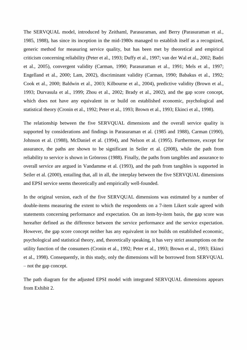
The SERVQUAL model, introduced by Zeithaml, Parasuraman, and Berry (Parasuraman et al.,
1985, 1988), has since its inception in the mid-1980s managed to establish itself as a recognized,
generic method for measuring service quality, but has been met by theoretical and empirical
criticism concerning reliability (Peter et al., 1993; Duffy et al., 1997; van der Wal et al., 2002; Badri
et al., 2005), convergent validity (Carman, 1990; Parasuraman et al., 1991; Mels et al., 1997;
Engelland et al., 2000; Lam, 2002), discriminant validity (Carman, 1990; Babakus et al., 1992;
Cook et al., 2000; Baldwin et al., 2003; Kilbourne et al., 2004), predictive validity (Brown et al.,
1993; Durvasula et al., 1999; Zhou et al., 2002; Brady et al., 2002), and the gap score concept,
which does not have any equivalent in or build on established economic, psychological and
statistical theory (Cronin et al., 1992; Peter et al., 1993; Brown et al., 1993; Ekinci et al., 1998).
The relationship between the five SERVQUAL dimensions and the overall service quality is
supported by considerations and findings in Parasuraman et al. (1985 and 1988), Carman (1990),
Johnson et al. (1988), McDaniel et al. (1994), and Nelson et al. (1995). Furthermore, except for
assurance, the paths are shown to be significant in Seiler et al. (2008), while the path from
reliability to service is shown in Grönross (1988). Finally, the paths from tangibles and assurance to
overall service are argued in Vandamme et al. (1993), and the path from tangibles is supported in
Seiler et al. (2000), entailing that, all in all, the interplay between the five SERVQUAL dimensions
and EPSI service seems theoretically and empirically well-founded.
In the original version, each of the five SERVQUAL dimensions was estimated by a number of
double-items measuring the extent to which the respondents on a 7-item Likert scale agreed with
statements concerning performance and expectation. On an item-by-item basis, the gap score was
hereafter defined as the difference between the service performance and the service expectation.
However, the gap score concept neither has any equivalent in nor builds on established economic,
psychological and statistical theory, and, theoretically speaking, it has very strict assumptions on the
utility function of the consumers (Cronin et al., 1992; Peter et al., 1993; Brown et al., 1993; Ekinci
et al., 1998). Consequently, in this study, only the dimensions will be borrowed from SERVQUAL
– not the gap concept.
The path diagram for the adjusted EPSI model with integrated SERVQUAL dimensions appears
from Exhibit 2.
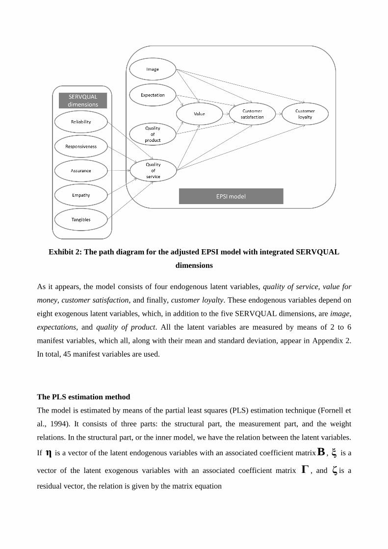
Exhibit 2: The path diagram for the adjusted EPSI model with integrated SERVQUAL
dimensions
As it appears, the model consists of four endogenous latent variables, quality of service, value for
money, customer satisfaction, and finally, customer loyalty. These endogenous variables depend on
eight exogenous latent variables, which, in addition to the five SERVQUAL dimensions, are image,
expectations, and quality of product. All the latent variables are measured by means of 2 to 6
manifest variables, which all, along with their mean and standard deviation, appear in Appendix 2.
In total, 45 manifest variables are used.
The PLS estimation method
The model is estimated by means of the partial least squares (PLS) estimation technique (Fornell et
al., 1994). It consists of three parts: the structural part, the measurement part, and the weight
relations. In the structural part, or the inner model, we have the relation between the latent variables.
If η is a vector of the latent endogenous variables with an associated coefficient matrixB , ξ is a
vector of the latent exogenous variables with an associated coefficient matrix Γ , and ζ is a
residual vector, the relation is given by the matrix equation

ζΓξBηη
The other part of the PLS model is the measurement model or the outer part, which defines the
relation between the latent and the manifest variables. In PLS, these outer relations can be reflective
as well as formative (Jöreskog et al., 1982). If y and x are vectors of the observed η and ξ
indicators, respectively, and y
Λ and x
Λ are the matrices that contain the iλ coefficients
combining the latent and manifest variables, the general equations for reflective external relations
are:
yyεηΛy
xxεξΛx
In these equations, yε and
xε designate the error vectors for y andx , respectively.
In the final part of a PLS model – the weight relations – η̂ and ξ̂ are estimates of η and ξ ,
respectively, and given as linear sums of the empirical indicators:
yωηη
ˆ
xωξξ
ˆ
The PLS algorithm consists of the following three steps:
1. Estimate weight relations of the measurement model via the PLS algorithm.
2. Estimate values of latent variables based on the weights from step 1.
3. Estimate the structural parameters based on the latent variable values estimated in step 2.
PLS is a correlation-based estimation technique in the sense that the relations between the latent
variables, given as a linear combination of the manifest variables, are estimated in such a way that
the exogenous latent variables are maximally correlated with the endogenous latent variables in the
system. As opposed to the covariance-based method, also known as LISREL-type modeling, in PLS
the weights are the rescaled loadings from a principal component analysis.
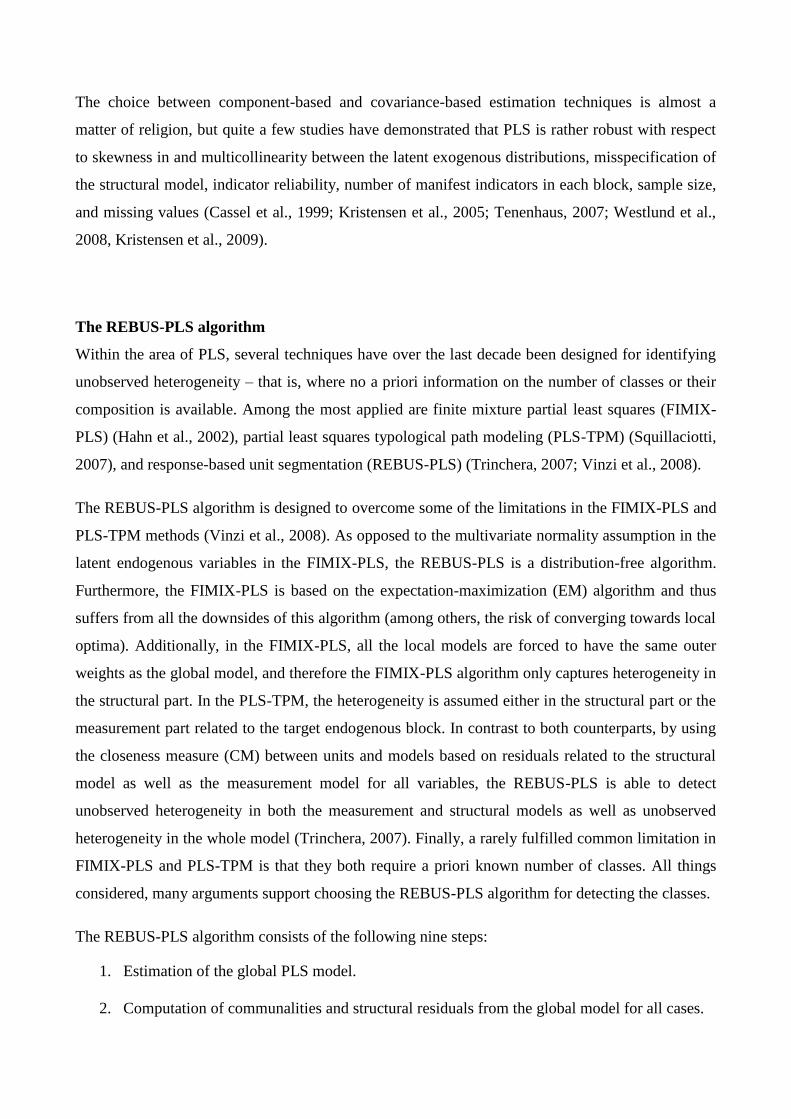
The choice between component-based and covariance-based estimation techniques is almost a
matter of religion, but quite a few studies have demonstrated that PLS is rather robust with respect
to skewness in and multicollinearity between the latent exogenous distributions, misspecification of
the structural model, indicator reliability, number of manifest indicators in each block, sample size,
and missing values (Cassel et al., 1999; Kristensen et al., 2005; Tenenhaus, 2007; Westlund et al.,
2008, Kristensen et al., 2009).
The REBUS-PLS algorithm
Within the area of PLS, several techniques have over the last decade been designed for identifying
unobserved heterogeneity – that is, where no a priori information on the number of classes or their
composition is available. Among the most applied are finite mixture partial least squares (FIMIX-
PLS) (Hahn et al., 2002), partial least squares typological path modeling (PLS-TPM) (Squillaciotti,
2007), and response-based unit segmentation (REBUS-PLS) (Trinchera, 2007; Vinzi et al., 2008).
The REBUS-PLS algorithm is designed to overcome some of the limitations in the FIMIX-PLS and
PLS-TPM methods (Vinzi et al., 2008). As opposed to the multivariate normality assumption in the
latent endogenous variables in the FIMIX-PLS, the REBUS-PLS is a distribution-free algorithm.
Furthermore, the FIMIX-PLS is based on the expectation-maximization (EM) algorithm and thus
suffers from all the downsides of this algorithm (among others, the risk of converging towards local
optima). Additionally, in the FIMIX-PLS, all the local models are forced to have the same outer
weights as the global model, and therefore the FIMIX-PLS algorithm only captures heterogeneity in
the structural part. In the PLS-TPM, the heterogeneity is assumed either in the structural part or the
measurement part related to the target endogenous block. In contrast to both counterparts, by using
the closeness measure (CM) between units and models based on residuals related to the structural
model as well as the measurement model for all variables, the REBUS-PLS is able to detect
unobserved heterogeneity in both the measurement and structural models as well as unobserved
heterogeneity in the whole model (Trinchera, 2007). Finally, a rarely fulfilled common limitation in
FIMIX-PLS and PLS-TPM is that they both require a priori known number of classes. All things
considered, many arguments support choosing the REBUS-PLS algorithm for detecting the classes.
The REBUS-PLS algorithm consists of the following nine steps:
1. Estimation of the global PLS model.
2. Computation of communalities and structural residuals from the global model for all cases.

3. Hierarchical clustering based on the communalities and residuals from step 2.
4. Choice of the number of segments, K, based on the dendrogram prepared in step 3.
5. Assignment of all cases to each segment, based on the clustering analysis.
6. Estimation of the K local models.
7. Computation of the closeness measure (CM) for each case with respect to each local model.
8. Assignment of each case to the closest local model.
If the segment membership is stable, proceed to step 9; if not, go back to step 6.
9. Description of the obtained segments according to differences among the local models.
In a PLS path model, the overall measure of model performance is the global criterion of goodness
of fit proposed by Tenenhaus et al. (2004). The index is a measure that takes into account the model
performance in both the measurement part and the structural part of the model. It is computed as the
geometrical average of the average R2 values from the structural model and the weighted average
communality index from the measurement model, where the number of manifest variables of each
block is used as weight:
GoFabsolute = √𝑅2̅̅̅̅ ∙ Communality̅̅ ̅̅ ̅̅ ̅̅ ̅̅ ̅̅ ̅̅ ̅̅ ̅
It can be written as:
𝐺𝑜𝐹 = √1
𝑃∑∑(1 −
∑ 𝑒𝑖 𝑝𝑞2𝑁
𝑖=1
∑ (𝑥𝑖 𝑝𝑞 − �̅�𝑝𝑞)2𝑁
𝑖=1
) ∙1
𝐽∑(1 −
∑ 𝑓𝑖𝑗2𝑁
𝑖=1
∑ (𝜉𝑖𝑗 − 𝜉�̅�)2𝑁
𝑖=1
)
𝐽
𝑗=1
𝑃𝑞
𝑝=1
𝑄
𝑞=1
P, Q and J stand, respectively, for the number of manifest, latent, and endogenous variables in the
model, f is the communalities, and e is the structural residuals.
For the purpose of assessing the quality of the group separation and performance of the local
models compared to the global model, the Group Quality Index (GQI) introduced in Trinchera
(2007) will be used:
𝐺𝑄𝐼 = √∑𝑛𝑘𝑁
𝐾
𝑘=1
[1
𝑃∑∑(1−
∑ 𝑒𝑖 𝑝𝑞𝑘2𝑛𝑘
𝑖=1
∑ (𝑥𝑖 𝑝𝑞 − �̅�𝑝𝑞𝑘)2𝑛𝑘
𝑖=1
)] ∙∑𝑛𝑘𝑁
𝐾
𝑘=1
[1
𝐽∑(1 −
∑ 𝑓𝑖𝑗𝑘2𝑛𝑘
𝑖=1
∑ (𝜉𝑖𝑗𝑘 − 𝜉�̅�𝑘)2𝑛𝑘
𝑖=1
)
𝐽
𝑗=1
]
𝑃𝑞
𝑝=1
𝑄
𝑞=1
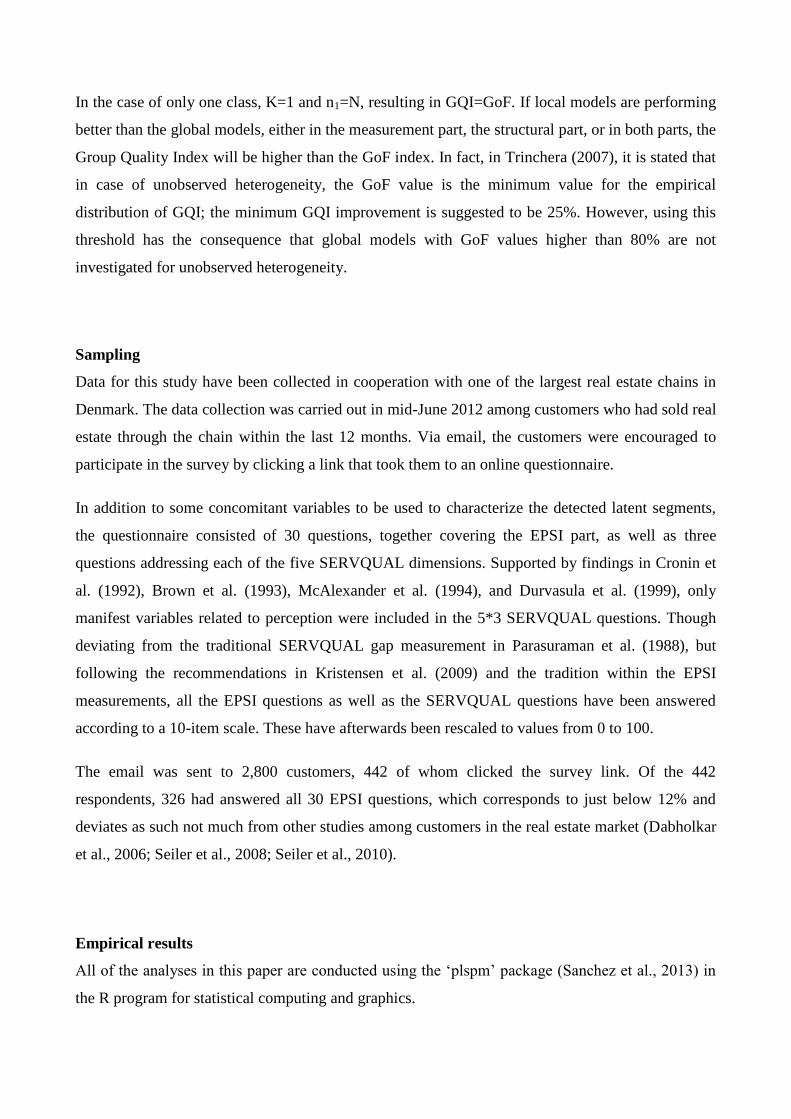
In the case of only one class, K=1 and n1=N, resulting in GQI=GoF. If local models are performing
better than the global models, either in the measurement part, the structural part, or in both parts, the
Group Quality Index will be higher than the GoF index. In fact, in Trinchera (2007), it is stated that
in case of unobserved heterogeneity, the GoF value is the minimum value for the empirical
distribution of GQI; the minimum GQI improvement is suggested to be 25%. However, using this
threshold has the consequence that global models with GoF values higher than 80% are not
investigated for unobserved heterogeneity.
Sampling
Data for this study have been collected in cooperation with one of the largest real estate chains in
Denmark. The data collection was carried out in mid-June 2012 among customers who had sold real
estate through the chain within the last 12 months. Via email, the customers were encouraged to
participate in the survey by clicking a link that took them to an online questionnaire.
In addition to some concomitant variables to be used to characterize the detected latent segments,
the questionnaire consisted of 30 questions, together covering the EPSI part, as well as three
questions addressing each of the five SERVQUAL dimensions. Supported by findings in Cronin et
al. (1992), Brown et al. (1993), McAlexander et al. (1994), and Durvasula et al. (1999), only
manifest variables related to perception were included in the 5*3 SERVQUAL questions. Though
deviating from the traditional SERVQUAL gap measurement in Parasuraman et al. (1988), but
following the recommendations in Kristensen et al. (2009) and the tradition within the EPSI
measurements, all the EPSI questions as well as the SERVQUAL questions have been answered
according to a 10-item scale. These have afterwards been rescaled to values from 0 to 100.
The email was sent to 2,800 customers, 442 of whom clicked the survey link. Of the 442
respondents, 326 had answered all 30 EPSI questions, which corresponds to just below 12% and
deviates as such not much from other studies among customers in the real estate market (Dabholkar
et al., 2006; Seiler et al., 2008; Seiler et al., 2010).
Empirical results
All of the analyses in this paper are conducted using the ‘plspm’ package (Sanchez et al., 2013) in
the R program for statistical computing and graphics.

All the blocks are measured reflectively and should, as such, reflect the unique latent construct –
therefore, the blocks should be unidimensional and homogeneous (Vinzi et al., 2010). The
correlations between the manifest and latent variables appear in Appendix 1and from Exhibit 3, we
see that the smallest Dillon-Goldstein’s (or Jöreskog’s) rho is 0.935 and thus exceeds the threshold
of 0.7 recommended by Chin (1998); consequently, the blocks are considered homogenous.
Moreover, the classical measure of internal consistency in reliability analysis, Cronbach’s alpha, is
at least 0.896, which strongly supports the homogeneity claim. Since the Dillon-Goldstein’s rho, in
contrast to Cronbach’s alpha, does not assume that each manifest variable is equally important in
defining the latent construct (the so-called tau equivalence or parallelity), Dillon-Goldstein’s rho is
considered to be a better indicator of block homogeneity than Cronbach’s alpha.
With regard to the unidimensionality, only the first eigenvalue of the correlation matrix is greater
than 1; this being so, all blocks may be considered unidimensional according to Kaiser’s rule. All in
all, the blocks are homogeneous and unidimensional, indicating that the model is appropriate.
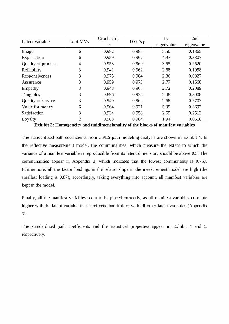
Latent variable # of MVs Cronbach’s
α D.G.’s ρ
1st
eigenvalue
2nd
eigenvalue
Image 6 0.982 0.985 5.50 0.1865
Expectation 6 0.959 0.967 4.97 0.3307
Quality of product 4 0.958 0.969 3.55 0.2520
Reliability 3 0.941 0.962 2.68 0.1958
Responsiveness 3 0.975 0.984 2.86 0.0827
Assurance 3 0.959 0.973 2.77 0.1668
Empathy 3 0.948 0.967 2.72 0.2089
Tangibles 3 0.896 0.935 2.48 0.3008
Quality of service 3 0.940 0.962 2.68 0.2703
Value for money 6 0.964 0.971 5.09 0.3697
Satisfaction 3 0.934 0.958 2.65 0.2513
Loyalty 2 0.968 0.984 1.94 0.0618
Exhibit 3: Homogeneity and unidimensionality of the blocks of manifest variables
The standardized path coefficients from a PLS path modeling analysis are shown in Exhibit 4. In
the reflective measurement model, the communalities, which measure the extent to which the
variance of a manifest variable is reproducible from its latent dimension, should be above 0.5. The
communalities appear in Appendix 3, which indicates that the lowest communality is 0.757.
Furthermore, all the factor loadings in the relationships in the measurement model are high (the
smallest loading is 0.87); accordingly, taking everything into account, all manifest variables are
kept in the model.
Finally, all the manifest variables seem to be placed correctly, as all manifest variables correlate
higher with the latent variable that it reflects than it does with all other latent variables (Appendix
3).
The standardized path coefficients and the statistical properties appear in Exhibit 4 and 5,
respectively.
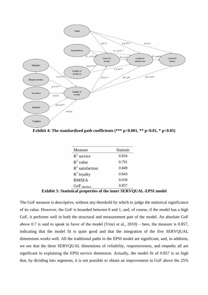
Exhibit 4: The standardized path coefficients (*** p<0.001, ** p<0.01, * p<0.05)
Measure Statistic
R2 service 0.834
R2 value 0.791
R2 satisfaction 0.849
R2 loyalty 0.843
RMSEA 0.039
GoF absolute 0.857
Exhibit 5: Statistical properties of the inner SERVQUAL-EPSI model
The GoF measure is descriptive, without any threshold by which to judge the statistical significance
of its value. However, the GoF is bounded between 0 and 1, and, of course, if the model has a high
GoF, it performs well in both the structural and measurement part of the model. An absolute GoF
above 0.7 is said to speak in favor of the model (Vinzi et al., 2010) – here, the measure is 0.857,
indicating that the model fit is quite good and that the integration of the five SERVQUAL
dimensions works well. All the traditional paths in the EPSI model are significant, and, in addition,
we see that the three SERVQUAL dimensions of reliability, responsiveness, and empathy all are
significant in explaining the EPSI service dimension. Actually, the model fit of 0.857 is so high
that, by dividing into segments, it is not possible to obtain an improvement in GoF above the 25%

threshold originally suggested by Trinchera (2007). So, if we were true to the origins and applied
the original decision rule, we would stop and be satisfied that only one segment exists.
However, there are several indications that, in this business, there exists heterogeneous customer
behavior and that the REBUS-PLS algorithm is suitable for detecting these:
Firstly, the answers to the satisfaction questions seem to be more diverse than traditionally seen in
satisfaction studies such as EPSI measurements. The sample size of 326 respondents gives a 95%
confidence interval for the mean satisfaction going from 70.6 to 76.1, so half of the width is 2.74.
Usually, a sample size of approximately 250 will ensure a half-width of maximum 2. Secondly,
since the reliability of the indicators is high and the specification error of the structural model is
low, the REBUS-PLS algorithm should be able to find a suitable segment solution (Eskildsen et al.,
2013).
As recommended in Eskildsen et al. (2013), four criteria should be used to find a suitable segment
solution:
1. Choose the first local maximum solution of the Group Quality Index.
2. At least one local model must have a higher GoF than the global model.
3. All path coefficients must retain the expected signs.
4. All local models must be significantly different.
As usual (Vinzi et al., 2008), stability in the algorithm is obtained after only a few iterations.
Exhibit 6 shows the Group Quality Index for different segment solutions, and the first local
maximum is for K=2 with a GQI=0.8715. The identified segments have GoF values of 0.899 and
0.828, respectively. Ergo, using criterion 1 to choose the number of segments fulfils criterion 2 as
well.
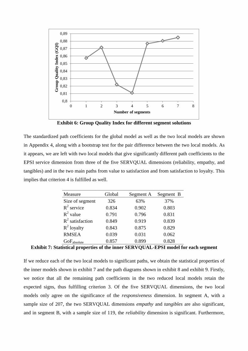
Exhibit 6: Group Quality Index for different segment solutions
The standardized path coefficients for the global model as well as the two local models are shown
in Appendix 4, along with a bootstrap test for the pair difference between the two local models. As
it appears, we are left with two local models that give significantly different path coefficients to the
EPSI service dimension from three of the five SERVQUAL dimensions (reliability, empathy, and
tangibles) and in the two main paths from value to satisfaction and from satisfaction to loyalty. This
implies that criterion 4 is fulfilled as well.
Measure Global Segment A Segment B
Size of segment 326 63% 37%
R2 service 0.834 0.902 0.803
R2 value 0.791 0.796 0.831
R2 satisfaction 0.849 0.919 0.839
R2 loyalty 0.843 0.875 0.829
RMSEA 0.039 0.031 0.062
GoFabsolute 0.857 0.899 0.828
Exhibit 7: Statistical properties of the inner SERVQUAL-EPSI model for each segment
If we reduce each of the two local models to significant paths, we obtain the statistical properties of
the inner models shown in exhibit 7 and the path diagrams shown in exhibit 8 and exhibit 9. Firstly,
we notice that all the remaining path coefficients in the two reduced local models retain the
expected signs, thus fulfilling criterion 3. Of the five SERVQUAL dimensions, the two local
models only agree on the significance of the responsiveness dimension. In segment A, with a
sample size of 207, the two SERVQUAL dimensions empathy and tangibles are also significant,
and in segment B, with a sample size of 119, the reliability dimension is significant. Furthermore,
0,8
0,81
0,82
0,83
0,84
0,85
0,86
0,87
0,88
0,89
0 1 2 3 4 5 6 7 8
Gro
up
Qu
ali
ty I
nd
ex (
GQ
I)
Number of segments
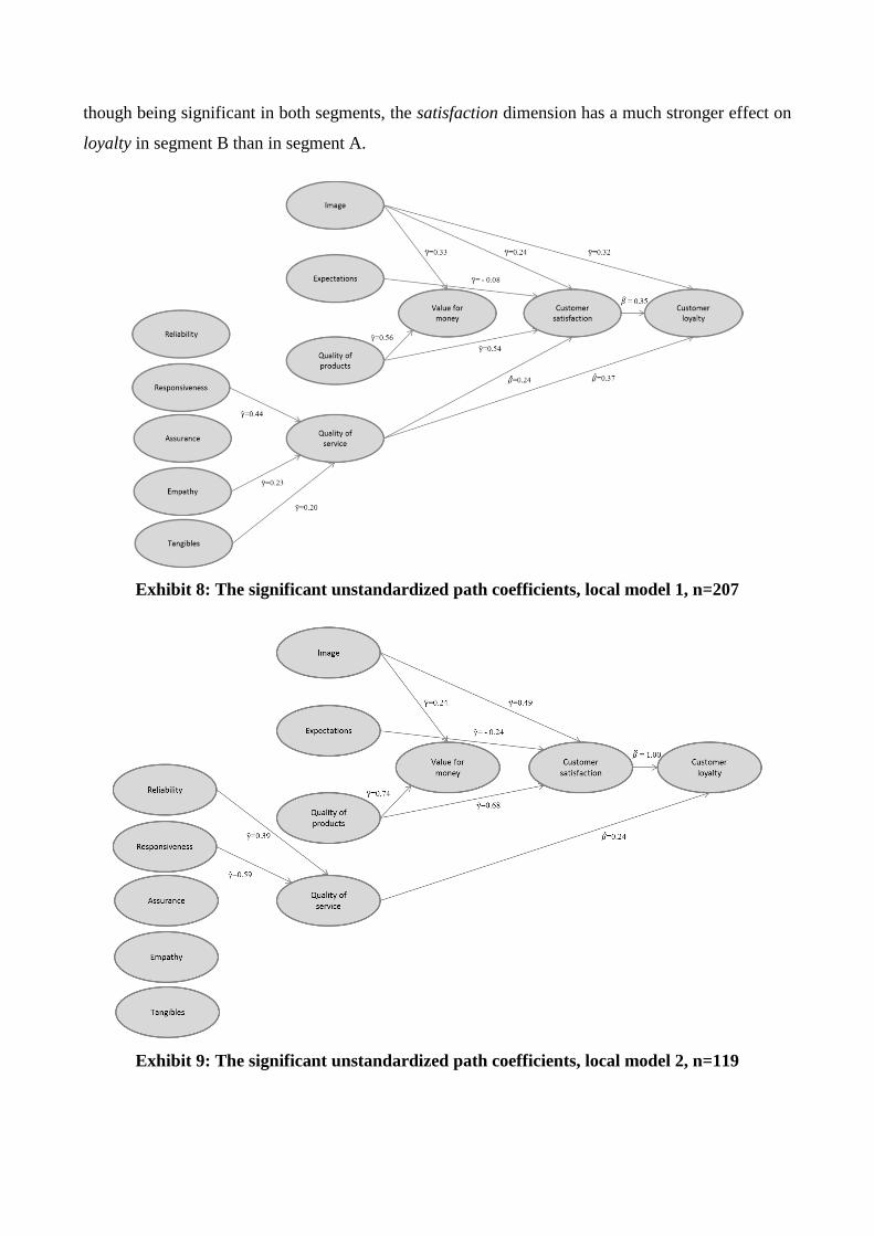
though being significant in both segments, the satisfaction dimension has a much stronger effect on
loyalty in segment B than in segment A.
Exhibit 8: The significant unstandardized path coefficients, local model 1, n=207
Exhibit 9: The significant unstandardized path coefficients, local model 2, n=119
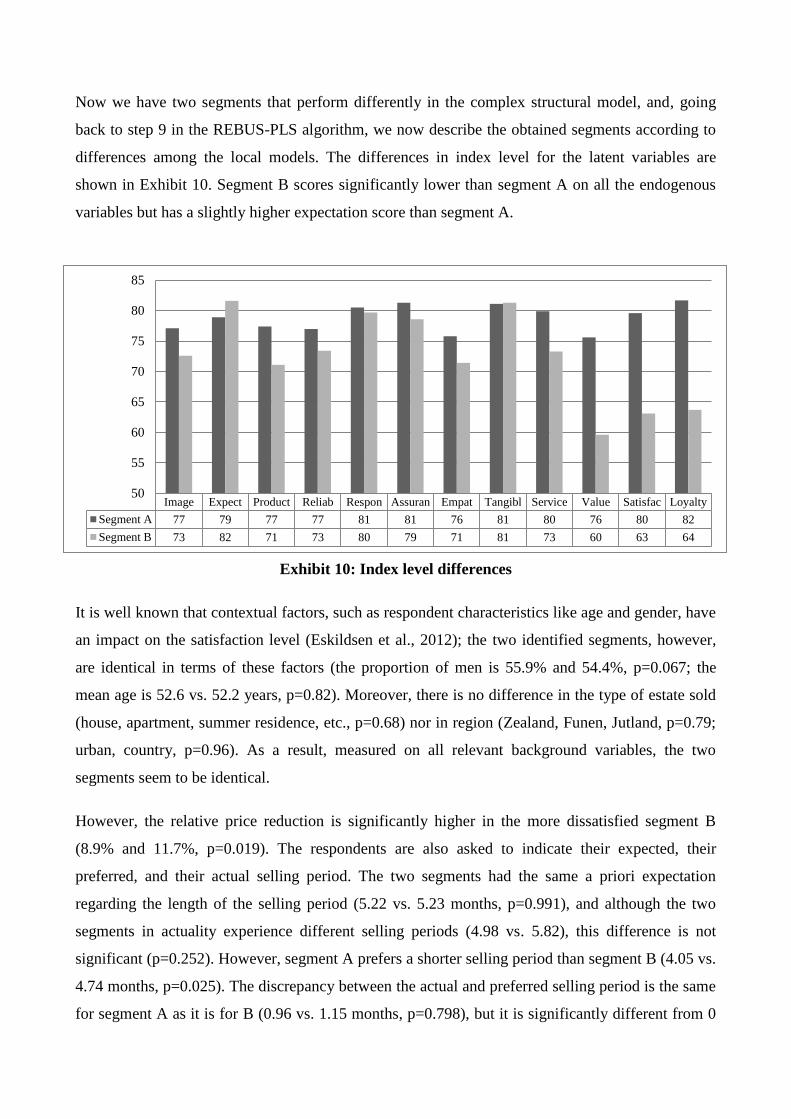
Image Expect Product Reliab Respon Assuran Empat Tangibl Service Value Satisfac Loyalty
Segment A 77 79 77 77 81 81 76 81 80 76 80 82
Segment B 73 82 71 73 80 79 71 81 73 60 63 64
50
55
60
65
70
75
80
85
Now we have two segments that perform differently in the complex structural model, and, going
back to step 9 in the REBUS-PLS algorithm, we now describe the obtained segments according to
differences among the local models. The differences in index level for the latent variables are
shown in Exhibit 10. Segment B scores significantly lower than segment A on all the endogenous
variables but has a slightly higher expectation score than segment A.
Exhibit 10: Index level differences
It is well known that contextual factors, such as respondent characteristics like age and gender, have
an impact on the satisfaction level (Eskildsen et al., 2012); the two identified segments, however,
are identical in terms of these factors (the proportion of men is 55.9% and 54.4%, p=0.067; the
mean age is 52.6 vs. 52.2 years, p=0.82). Moreover, there is no difference in the type of estate sold
(house, apartment, summer residence, etc., p=0.68) nor in region (Zealand, Funen, Jutland, p=0.79;
urban, country, p=0.96). As a result, measured on all relevant background variables, the two
segments seem to be identical.
However, the relative price reduction is significantly higher in the more dissatisfied segment B
(8.9% and 11.7%, p=0.019). The respondents are also asked to indicate their expected, their
preferred, and their actual selling period. The two segments had the same a priori expectation
regarding the length of the selling period (5.22 vs. 5.23 months, p=0.991), and although the two
segments in actuality experience different selling periods (4.98 vs. 5.82), this difference is not
significant (p=0.252). However, segment A prefers a shorter selling period than segment B (4.05 vs.
4.74 months, p=0.025). The discrepancy between the actual and preferred selling period is the same
for segment A as it is for B (0.96 vs. 1.15 months, p=0.798), but it is significantly different from 0
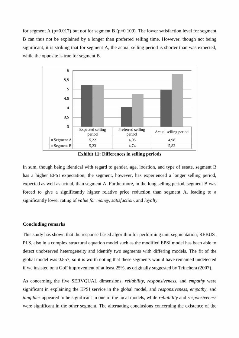
for segment A (p=0.017) but not for segment B (p=0.109). The lower satisfaction level for segment
B can thus not be explained by a longer than preferred selling time. However, though not being
significant, it is striking that for segment A, the actual selling period is shorter than was expected,
while the opposite is true for segment B.
Exhibit 11: Differences in selling periods
In sum, though being identical with regard to gender, age, location, and type of estate, segment B
has a higher EPSI expectation; the segment, however, has experienced a longer selling period,
expected as well as actual, than segment A. Furthermore, in the long selling period, segment B was
forced to give a significantly higher relative price reduction than segment A, leading to a
significantly lower rating of value for money, satisfaction, and loyalty.
Concluding remarks
This study has shown that the response-based algorithm for performing unit segmentation, REBUS-
PLS, also in a complex structural equation model such as the modified EPSI model has been able to
detect unobserved heterogeneity and identify two segments with differing models. The fit of the
global model was 0.857, so it is worth noting that these segments would have remained undetected
if we insisted on a GoF improvement of at least 25%, as originally suggested by Trinchera (2007).
As concerning the five SERVQUAL dimensions, reliability, responsiveness, and empathy were
significant in explaining the EPSI service in the global model, and responsiveness, empathy, and
tangibles appeared to be significant in one of the local models, while reliability and responsiveness
were significant in the other segment. The alternating conclusions concerning the existence of the
Expected selling
period
Preferred selling
periodActual selling period
Segment A 5,22 4,05 4,98
Segment B 5,23 4,74 5,82
3
3,5
4
4,5
5
5,5
6

SERVQUAL dimensions in the real estate business (McDaniel et al., 1994; Seiler et al., 2000;
Seiler et al., 2008) can now be seen as a result of the existence of different segments.

Appendix 1: Correlations between the manifest and latent variables
Image Expec Product Reliability Respon Assurance Empathy Tangibles Service Value Sat Loyalty
Image1 0.936 0.472 0.821 0.836 0.791 0.804 0.828 0.736 0.809 0.749 0.805 0.789
Image2 0.958 0.503 0.828 0.831 0.783 0.818 0.847 0.736 0.832 0.771 0.810 0.777
Image3 0.945 0.497 0.835 0.777 0.732 0.763 0.795 0.685 0.821 0.805 0.811 0.783
Image4 0.950 0.528 0.836 0.789 0.774 0.804 0.790 0.738 0.837 0.781 0.823 0.790
Image5 0.972 0.500 0.850 0.826 0.811 0.814 0.817 0.746 0.867 0.799 0.837 0.805
Image6 0.981 0.504 0.863 0.843 0.802 0.814 0.837 0.737 0.859 0.814 0.849 0.822
Exp1 0.507 0.919 0.518 0.467 0.436 0.476 0.494 0.535 0.466 0.399 0.395 0.333
Exp2 0.519 0.927 0.488 0.454 0.433 0.457 0.469 0.515 0.473 0.369 0.404 0.358
Exp3 0.416 0.903 0.463 0.396 0.432 0.440 0.408 0.501 0.459 0.357 0.347 0.281
Exp4 0.407 0.876 0.463 0.397 0.400 0.428 0.408 0.478 0.421 0.329 0.319 0.270
Exp5 0.470 0.874 0.464 0.378 0.378 0.407 0.383 0.481 0.430 0.350 0.365 0.302
Exp6 0.522 0.958 0.544 0.452 0.449 0.493 0.478 0.542 0.502 0.409 0.413 0.346
Product1 0.843 0.503 0.962 0.845 0.832 0.827 0.843 0.765 0.911 0.852 0.883 0.833
Product2 0.807 0.499 0.927 0.823 0.808 0.815 0.811 0.708 0.874 0.813 0.814 0.788
Product3 0.780 0.547 0.908 0.807 0.820 0.801 0.806 0.786 0.839 0.768 0.781 0.750
Product4 0.870 0.492 0.971 0.869 0.865 0.878 0.868 0.773 0.951 0.865 0.902 0.868
Reliability1 0.814 0.473 0.843 0.954 0.854 0.867 0.855 0.773 0.814 0.766 0.793 0.746
Reliability2 0.841 0.440 0.854 0.951 0.854 0.850 0.842 0.757 0.845 0.790 0.829 0.779
Reliability3 0.766 0.414 0.821 0.932 0.894 0.863 0.849 0.805 0.824 0.746 0.764 0.734
Respon.1 0.808 0.472 0.861 0.900 0.979 0.913 0.888 0.839 0.872 0.745 0.785 0.747
Respon.2 0.805 0.455 0.865 0.905 0.977 0.891 0.876 0.847 0.894 0.780 0.810 0.770
Respon.3 0.779 0.430 0.856 0.879 0.972 0.907 0.871 0.820 0.861 0.770 0.775 0.741
Assurance1 0.827 0.469 0.844 0.886 0.878 0.972 0.883 0.798 0.839 0.751 0.814 0.775
Assurance2 0.796 0.480 0.849 0.859 0.863 0.968 0.861 0.790 0.820 0.734 0.793 0.757
Assurance3 0.794 0.481 0.849 0.875 0.926 0.944 0.858 0.845 0.842 0.741 0.774 0.731
Empathy1 0.794 0.472 0.840 0.862 0.861 0.864 0.967 0.815 0.824 0.738 0.774 0.740
Empathy2 0.833 0.487 0.867 0.880 0.916 0.892 0.963 0.848 0.854 0.763 0.791 0.762
Empathy3 0.818 0.427 0.815 0.819 0.789 0.821 0.926 0.738 0.809 0.755 0.801 0.791

Image Expec Product Reliability Respon Assurance Empathy Tangibles Service Value Sat Loyalty
Tangibles1 0.617 0.541 0.654 0.676 0.714 0.687 0.721 0.890 0.662 0.542 0.566 0.520
Tangibles2 0.792 0.504 0.828 0.842 0.875 0.885 0.857 0.935 0.830 0.701 0.756 0.724
Tangibles3 0.651 0.489 0.693 0.708 0.729 0.709 0.702 0.902 0.693 0.581 0.636 0.587
Service1 0.876 0.464 0.924 0.871 0.857 0.846 0.847 0.758 0.966 0.849 0.909 0.872
Service2 0.716 0.498 0.821 0.730 0.811 0.735 0.744 0.759 0.896 0.733 0.709 0.686
Service3 0.879 0.476 0.943 0.872 0.876 0.874 0.874 0.777 0.973 0.850 0.897 0.867
Value1 0.705 0.338 0.743 0.709 0.657 0.665 0.693 0.563 0.716 0.877 0.728 0.688
Value2 0.774 0.362 0.842 0.772 0.759 0.761 0.770 0.636 0.838 0.943 0.811 0.782
Value3 0.695 0.400 0.733 0.682 0.698 0.633 0.658 0.612 0.766 0.870 0.690 0.663
Value4 0.777 0.390 0.831 0.773 0.736 0.727 0.719 0.634 0.797 0.928 0.772 0.740
Value5 0.768 0.372 0.821 0.733 0.710 0.703 0.730 0.611 0.779 0.932 0.778 0.757
Value6 0.814 0.387 0.860 0.805 0.764 0.768 0.786 0.667 0.844 0.970 0.844 0.818
Sat1 0.709 0.345 0.735 0.695 0.667 0.680 0.680 0.606 0.731 0.679 0.902 0.762
Sat2 0.839 0.399 0.876 0.818 0.782 0.799 0.800 0.702 0.872 0.820 0.962 0.897
Sat3 0.864 0.414 0.909 0.847 0.822 0.837 0.843 0.727 0.896 0.852 0.955 0.897
Loyal1 0.792 0.328 0.828 0.774 0.744 0.755 0.772 0.658 0.831 0.783 0.878 0.984
Loyal2 0.841 0.357 0.866 0.793 0.774 0.791 0.807 0.678 0.861 0.806 0.913 0.985
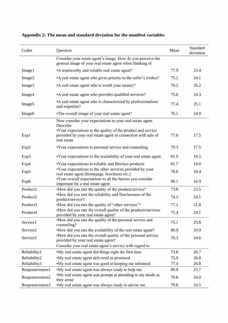
Appendix 2: The mean and standard deviation for the manifest variables
Codes Question Mean Standard
deviation
Consider your estate agent’s image. How do you perceive the
general image of your real estate agent when thinking of
Image1 •A trustworthy and reliable real estate agent? 77.9 23.4
Image2 •A real estate agent who gives priority to the seller’s wishes? 75.2 24.1
Image3 •A real estate agent who is worth your money? 70.2 26.2
Image4 •A real estate agent who provides qualified services? 75.6 24.3
Image5 •A real estate agent who is characterized by professionalism
and expertise? 77.4 25.1
Image6 •The overall image of your real estate agent? 76.1 24.9
Now consider your expectations to your real estate agent.
Describe
Exp1
•Your expectations to the quality of the product and service
provided by your real estate agent in connection with sale of
real estate
77.8 17.5
Exp2 •Your expectations to personal service and counseling 79.3 17.5
Exp3 •Your expectations to the availability of your real estate agent 81.9 16.5
Exp4 •Your expectations to reliable and flawless products 81.7 18.0
Exp5 •Your expectations to the other services provided by your
real estate agent (homepage, brochures etc.) 78.6 18.4
Exp6 •Your overall expectations to all the factors you consider
important for a real estate agent 80.1 16.9
Product1 •How did you rate the quality of the product/service? 73.8 23.5
Product2 •How did you rate the reliability and flawlessness of the
product/service? 74.2 24.1
Product3 •How did you rate the quality of “other services”? 77.1 21.8
Product4 •How did you rate the overall quality of the products/services
provided by your real estate agent? 75.4 24.1
Service1 •How did you rate the quality of the personal service and
counseling? 75.1 25.8
Service2 •How did you rate the availability of the real estate agent? 80.9 20.9
Service3 •How did you rate the overall quality of the personal service
provided by your real estate agent? 76.3 24.6
Consider your real estate agent’s service with regard to
Reliability1 •My real estate agent did things right the first time 73.8 26.7
Reliability2 •My real estate agent delivered as promised 75.9 26.8
Reliability3 •My real estate agent was good at keeping me informed 77.4 26.8
Responsiveness1 •My real estate agent was always ready to help me 80.8 23.7
Responsiveness2 •My real estate agent was prompt at attending to my needs as
they arose 79.8 24.0
Responsiveness3 •My real estate agent was always ready to advise me 79.8 24.5

Codes Question Mean Standard
deviation
Assurance1 •I trusted my real estate agent 79.8 25.3
Assurance2 •I trusted that my real estate agent handled everything
correctly 79.8 25.0
Assurance3 •The real estate agent was always capable of answering my
questions 81.1 23.2
Empathy1 •My needs were the focal point for the estate agent 75.1 24.9
Empathy2 •The real estate agent was committed to helping me 78.2 24.4
Empathy3 •My real estate agent did what was best for me – not what
was best for the agent’s earnings 68.3 27.9
Tangibles1 •My real estate agent had convenient business hours 81.0 20.6
Tangibles2 •The real estate agent had a professional appearance 81.9 22.5
Tangibles3 •My real estate agent’s homepage, brochures and other
information material appealed to me 80.5 20.6
Consider your sale and the personal service at your real estate agent.
How do you rate the value of those two in relation to what you paid
Value1 •In relation to the sales result (sales price, price reduction,
other terms)? 62.7 26.5
Value2 •In relation to personal service and counseling? 68.5 27.3
Value3 •In relation to the availability of the real estate agent? 78.2 23.0
Value4 •In relation to a reliable and flawless product/service? 71.5 26.6
Value5 •In relation to the other services provided by your real estate
agent? 68.8 26.2
Value6 •The overall value for money? 69.0 25.8
Sat1 •On the basis of your overall experience with your real estate
agent, how satisfied are you altogether? 73.0 28.6
Sat2 •Imagine the ideal real estate agent – how far from or how
close to this ideal is your real estate agent? 74.5 26.1
Sat3 •How well do you think your real estate agent managed to
meet your overall expectations? 72.6 25.9
Loyal1
•If you were to sell a property today, how certain are you that
you would choose the same real estate agent/estate agency
chain as the last time?
74.4 30.0
Loyal2 •Would you recommend the real estate agent to friends and
colleagues? 75.9 30.6
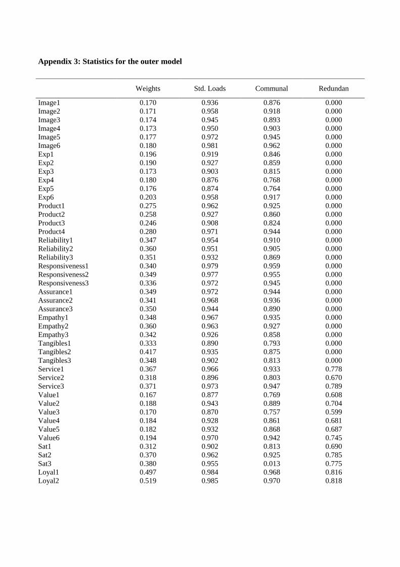
Appendix 3: Statistics for the outer model
Weights Std. Loads Communal Redundan
Image1 0.170 0.936 0.876 0.000
Image2 0.171 0.958 0.918 0.000
Image3 0.174 0.945 0.893 0.000
Image4 0.173 0.950 0.903 0.000
Image5 0.177 0.972 0.945 0.000
Image6 0.180 0.981 0.962 0.000
Exp1 0.196 0.919 0.846 0.000
Exp2 0.190 0.927 0.859 0.000
Exp3 0.173 0.903 0.815 0.000
Exp4 0.180 0.876 0.768 0.000
Exp5 0.176 0.874 0.764 0.000
Exp6 0.203 0.958 0.917 0.000
Product1 0.275 0.962 0.925 0.000
Product2 0.258 0.927 0.860 0.000
Product3 0.246 0.908 0.824 0.000
Product4 0.280 0.971 0.944 0.000
Reliability1 0.347 0.954 0.910 0.000
Reliability2 0.360 0.951 0.905 0.000
Reliability3 0.351 0.932 0.869 0.000
Responsiveness1 0.340 0.979 0.959 0.000
Responsiveness2 0.349 0.977 0.955 0.000
Responsiveness3 0.336 0.972 0.945 0.000
Assurance1 0.349 0.972 0.944 0.000
Assurance2 0.341 0.968 0.936 0.000
Assurance3 0.350 0.944 0.890 0.000
Empathy1 0.348 0.967 0.935 0.000
Empathy2 0.360 0.963 0.927 0.000
Empathy3 0.342 0.926 0.858 0.000
Tangibles1 0.333 0.890 0.793 0.000
Tangibles2 0.417 0.935 0.875 0.000
Tangibles3 0.348 0.902 0.813 0.000
Service1 0.367 0.966 0.933 0.778
Service2 0.318 0.896 0.803 0.670
Service3 0.371 0.973 0.947 0.789
Value1 0.167 0.877 0.769 0.608
Value2 0.188 0.943 0.889 0.704
Value3 0.170 0.870 0.757 0.599
Value4 0.184 0.928 0.861 0.681
Value5 0.182 0.932 0.868 0.687
Value6 0.194 0.970 0.942 0.745
Sat1 0.312 0.902 0.813 0.690
Sat2 0.370 0.962 0.925 0.785
Sat3 0.380 0.955 0.013 0.775
Loyal1 0.497 0.984 0.968 0.816
Loyal2 0.519 0.985 0.970 0.818
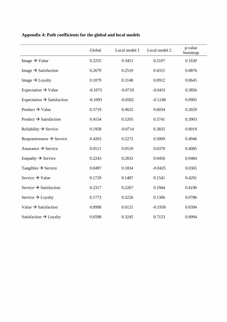
Appendix 4: Path coefficients for the global and local models
Global Local model 1 Local model 2
p-value
bootstrap
Image Value 0.2255 0.3451 0.2107 0.1630
Image Satisfaction 0.2679 0.2519 0.4315 0.0876
Image Loyalty 0.1079 0.3148 0.0912 0.0645
Expectation Value -0.1073 -0.0718 -0.0431 0.3856
Expectation Satisfaction -0.1093 -0.0502 -0.1248 0.0905
Product Value 0.5719 0.4625 0.6034 0.2659
Product Satisfaction 0.4154 0.5205 0.5741 0.3903
Reliability Service 0.1958 -0.0714 0.3835 0.0019
Responsiveness Service 0.4263 0.5272 0.5009 0.4946
Assurance Service 0.0511 0.0519 0.0370 0.4085
Empathy Service 0.2243 0.2833 0.0456 0.0484
Tangibles Service 0.0497 0.1834 -0.0425 0.0365
Service Value 0.1729 0.1487 0.1541 0.4291
Service Satisfaction 0.2317 0.2267 0.1944 0.4190
Service Loyalty 0.1773 0.3226 0.1306 0.0786
Value Satisfaction 0.0998 0.0121 -0.1958 0.0394
Satisfaction Loyalty 0.6598 0.3245 0.7153 0.0094
References
Babakus, E., Boller, G.W., 1992: An empirical assessment of the SERVQUAL scale, Journal of
Business Research, 1992, 24, 253-68.
Badri, M.A., Abdulla, M. and Al-Madani, A., 2005: Information technology center service quality:
assessment and application of SERVQUAL, International Journal of Quality & Reliability
Management, 22:8/9, pp. 819-48.
Baldwin, A. and Sohal, A. 2003: Service quality factors and outcomes in dental care”, Managing
Service Quality, 13:3, pp. 207-16.
Brady, M.K., Cronin, J.J. and Brand, R.R. 2002: Performance-only measurement of service quality:
a replication and extension, Journal of Business Research, 55:1, pp. 17-31.
Brown, T. J., Churchill, G.A. and Peter, J.P., 1993: Research note: improving the measurement of
service quality, Journal of Retailing, 69:1, pp. 127-39.
Carman, J.M., 1990: Consumer Perception of Service Quality: An assessment of the SERVQUAL
Dimensions, Journal of Retailing, Spring 1990, 66: 1, 33-55.
Cassel, C., Hackl, P., and Westlund, A.H., 1999: “Robustness of partial least-squares method for
estimating latent variables quality structures, Journal of Applied Statistics, 26:4, pp. 435-446.
Chin, W.W., 2008: The partial least squares method for structural equation modelling, in
G.A.Marcoulides(Ed), Modern methods for business research (pp. 295-236). London: Lawrence
Erlbaum Associates.
Cook, C. and Thompson, B., 2000: Reliability and validity of SERVQUAL scores used to evaluate
perceptions of library service quality, Journal of Academic Librarianship, 26:4, pp. 248-58.
Cronin, J. J., Taylor, S.A., 1992: Measuring Service Quality: A Reexamination and extension,
Journal of Marketing, July 1992, 56, pp. 55-68.
Dabholkar, P.A. and Overby, J.W., 2006: An Investigation of Real Estate Agent Service to Home
Sellers: Relevant Factors and Attributions, The Service Industries Journal, 26:5, pp. 557-579.
Duffy, J.A., Duffy, M. and Kilbourne, W., 1997: Cross national study of perceived service quality
in long-term care facilities, Journal of Aging Studies 11:4, pp. 327-36.
Durvasula, S., Lysonski, S. and Mehta, S.C., 1999: Testing the SERVQUAL scale in the business-
to-business sector: the case of ocean freight shipping service, Journal of Services Marketing, 13:2,
pp. 132-50.
Ekinci, Y., Riley, M., 1998: A critique of the issues and theoretical assumptions in service quality
measurement in the lodging industry: time to move the goal-posts, Hospitality Management, 17:4,
pp. 349-62.
Engelland, B.T., Workman, L. and Singh, M., 2000: Ensuring service quality for campus career
services centers: a modified SERVQUAL scale, Journal of Marketing Education, 22, pp. 236-45.
Eskildsen, J.K., Edgeman, R.; Kjærgaard, T., 2012: The Impact of Contextual factors on
Satisfaction: Consequences of Benchmarking Studies, on World Business Capability Congress,
New Zealand, 5-7/12 2012.
Eskildsen, J.K., Edgeman, R., Mønster, D. and Olesen, J.V., 2013: Response based segmentation in
satisfaction surveys, Performance Management Association Australia Conference 2013.
Fornell, C. 1992: A National Customer Satisfaction Barometer: The Swedish Experience, Journal of
Marketing, 56: January, pp. 6-21, 1992.
Fornell, C., Cha, J. 1994. Partial Least Squares. In Bagozzi, R.P. (Ed.), Advanced Methods of
Marketing Research. Blackwell, Cambridge, MA, pp. 52-78.
Grönross, C., 1998: The Six Criteria of Good Perceived Service Quality, Review of business, 1988,
9(3), pp. 10-13.
Hahn, C., Johnson, M.D., Herrmann, A. and Huber, F., 2002: Capturing Customer Heterogeneity
using a finite mixture PLS approach. Schmalenbach Business Review, 54, 243-269.
Jedidi, K., Jagpal, H.S. and S. De Sarbo, W., 1997: Finite-mixture structural equation models for
response-based segmentation and unobserved heterogeneity, Marketing Science 16:1, pp. 339-59.
Johnson, J. M., Nourse, H. O., Day, E., 1988: Factors related to selection of a Real Estate Agency
or Agent; The Journal of Real Estate Research, 3:2, pp. 109-118.
Jöreskog, K.G., and Wold, H., 1982: “The ML and PLS techniques for modeling with latent
variables”. In K.G. Jöreskog and H. Wold (Eds.), Systems under direct observations (pp.263-270),
New York: North Holland, 1982.
Kilbourne, W.E., Duffy, J.A., Duffy, M. and Giarchi, G. 2004: The applicability of SERVQUAL in
cross-national measurements of health-care quality, Journal of Services Marketing, 18: 6/7, pp. 524-
33.
Kristensen, K, Martensen, A. and Grønholdt, L., 2000: Customer satisfaction measurement at Post
Denmark: Results of application of the European Customer Satisfaction Index Methodology”, Total
Quality Management, 11, pp. 1007-1015.
Kristensen, K., Eskildsen, J., 2005: “PLS structural equation modeling for customer satisfaction
measurement: Some empirical and theoretical results”. In F.W.Bliemel, A.Eggert, G.Fassott, and
J.Henseler (Eds), Handbuch PLS-Pfadmodellierung-Methode, Praxisbeispiele, pp. 117-134,
Schäffer-Poeschel.
Kristensen, K., Eskildsen, J., 2009: “Design of PLS-satisfaction studies, In Handbook of Partial
Least Squares: Concepts, Methods and Applications in Marketing and Relates fields, Springer
Handbooks of Computational Statistics, eds. V.E.Vinzi, W.W.Chin, J.Henseler and H.Wang:
Springer Verlag.
Kristensen, K., Eskildsen, J.K., 2012: The relationship between SERVQUAL, National Customer
Satisfaction Indices, and Consumer Sentiment, The Quality Management Journal; 19: 2 pp. 47-61.
Lam, T.K.P. 2002: Making sense of SERVQUAL’s dimensions to the Chinese customers in Macau,
Journal of the Market-Focused Management, 5:10, pp. 43-58.
McAlexander, J.H., Kaldenberg, D.O. and Koenig, H.F., 1994: Service quality measurement:
examination of dental practices sheds more light on the relationships between service quality,
satisfaction, and purchase intensions in a health care setting, Journal of Health Care Marketing,
14:3, pp. 34-40.
McDaniel, J., M. Louargand, 1994: Real estate brokerage service quality: An examination, Journal
of Real Estate Research, 1994, 9:3, 339-351.
Mels, G., Boshoff, C. and Nel, D., 1997: The dimensions of service quality: the original European
perspective revisited, Service Industries Journal 17: 1, pp. 173-89.
Nelson, S.L. and Nelson, T.R., 1995: RESERV: an instrument for measuring real estate brokerage
service quality, Journal of Real Estate Research, 10: 1, pp. 99-113.
Parasuraman, A., Zeithaml., Berry, L., 1985: A Conceptual Model of Service Quality and its
implications for future Research, Journal of Marketing: fall, pp. 41-50.
Parasuraman, A. Zeithaml, V.A. and Berry, L.L. 1988: SERVQUAL: A multi-item scale for
measuring consumer perceptions of service quality, Journal of Retail, 64:1, pp. 12-40.
Parasuraman, A. Zeithaml, V.A. and Berry, L.L., 1991: Refinement and reassessment of the
SERVQUAL scale, Journal of Retailing, 67: 4, pp. 420-50.
Peter, J.P., Churchill, G.A. Jr and Brown, T.J., 1993: Caution in the use of difference scores in
consumer research, Journal of Consumer Research, 19: March, pp. 655-62.
Sanchez, G. and Trinchera, L. 2013: plspm: Tools for Partial Least Squares Path Modeling.
Seiler, V.; J. Webb, T. Whipple, 2000: Assessment of real estate brokerage service quality with a
practicing professional instrument, Journal of real estate research, 2000, 20:1/2, p. 105-117.
Seiler, V.; M. Seiler, D. Winkler, G. Newell, J. Webb, 2008: Service quality dimensions in
residential real estate brokerage, Journal of housing research, 2008, 17: 2, 101-116.
Seiler, V.; M. Seiler, A. Arndt, G. Newell, J. Webb, 2010: Measuring Service quality with
instrument variation in an SEM framework, Journal of Housing Research, 2010, 19: 1, p. 47-63.
Squillacciotti, S., 2007: Prediction-oriented classification in PLS path modeling. In: Vinzi, V.E.,
Chin, W. W., Henseler, J. and Wang, H. (eds.) Handbook of Partial Least Squares: Concepts,
Methods and Applications in Marketing and Related Fields, Springer Handbooks of Computational
Statistics. Springer Verlag.

Tenenhaus, Michel, 2007: A bridge between PLS path modelling and ULS-SEM, in “In honour of
Professor Kai Kristensen, Ledelse og økonomi, 2007.
Tenenhaus, M., Amato, S., and Esposito Vinzi, V. (2004): A Global goodness-of-fit index for PLS
structural equation modeling. Proceedings of the XLII SIS Scientific Meeting, Vol. Contributed
Papers, CLEUP, Padova, pp. 739-742.
Trinchera, L., 2007: Unobserved Heterogeneity in Structural Equation Models: a new approach to
latent class detection in PLS Path Modeling. PhD, Università degli Studi di Napoli Federico II.
Vandamme, R., Leunis, J. 1993: Development of a multi-Item scale for measuring hospital service
quality, International Journal of service Industry Management, 1993, 4: 3, 30-49.
van der Wal, R.W.E., Pampallis, A. and Bond, C., 2002: Service Quality in a cellular
telecommunications company: a South African experience, Managing Service Quality, 12(5), pp.
195-208.
Vinzi, V. E., Trinchera, L., Squillacciotti, S. and Tenenhaus, M., 2008: REBUS-PLS: A response-
based procedure for detecting unit segments in PLS path modelling, Applied Stochastic Models in
Business and Industry, 24, pp. 439-458.
Vinzi, V.E., Trinchera, L., Amato, S. 2010: PLS Path Modelling: From Foundations to Recent
Developments and Open Issues for Model Assessment and Improvement, In Handbook of Partial
Least Squares: Concepts, Methods and Applications in Marketing and Relates fields, Springer
Handbooks of Computational Statistics, eds. V.E.Vinzi, W.W.Chin, J.Henseler and H.Wang:
Springer Verlag.
Westlund, A.H., Källström, M., Parmler, J., 2008: SEM-based customer satisfaction measurement:
On multicollinearity and robust PLS estimation. Total Quality Management, 19: 7-8, 2008, pp. 855-
869.
Zhou, L., Zhang, Y. and Xu, J. 2002: A Critical Assessment of SERVQUAL’s Applicability in the
Banking Context of China, Asia Pacific Advances in Consumer Research, 5, Association for
Consumer Research, Valdosta, GA, pp. 14-21.
EPSI Measurement on Agent Performance
John Vestergaard Olesena*
and Jacob Kjær Eskildsen a
a ICOA, BTECH, Aarhus University
Birk Centerpark 15, 7400 Herning, Denmark
Keywords: Market research methodology, satisfaction, EPSI, buyer-seller duality.
Introduction
Since Fornell introduced a national customer satisfaction model in 1992 [1] , the EPSI model has
been applied in many different countries and sectors [2] , [3] , and the relation from customer
satisfaction and loyalty to financial performance is well-established [4] , [5] . We are now well
versed in the structure of the model and the level of indices [6] . However, contrary to previously
EPSI-studied businesses, the real estate business and others stand out since these businesses operate
with two types of “customers”; the seller who pays for the service and the buyer who, strictly
speaking, receives the service for free. It is not a problem to come up with two models and apply
the EPSI model on sellers as well as buyers. But, although these customers have a common interest
in concluding a deal, they have conflicting interests when it comes to price and terms. The
forthcoming study therefore simultaneously examines both sides of the coin.
Even though the real estate agent is the seller’s agent, he must also take measures to satisfy the
buyer, thus ensuring that he is in commission to sell and possibly also resell the property in the
future. Accordingly, the real estate agent faces the challenge of being able to simultaneously secure
a higher satisfaction level among both the buyer and the seller (Exhibit 1).

Exhibit 1: The buyer-seller-agent triangle
As a result, in the real estate business, the satisfaction concept becomes multidimensional at the
latent level, which entails some interesting challenges for the traditional EPSI model. This problem
is new in customer satisfaction measurement, and a coming case study will hopefully result in an
empirical model with reference to the EPSI model based on game- and agent-theoretical
considerations. Data come from a survey among buyer/seller pairs who, within the last three
months, all have sold real estate through DanBolig, one of the largest real estate chains in Denmark.
PLS path modeling [7] , [8] [9] will be applied to estimate the suggested relationships.
Analysis of dyadic data
In the presence of dyadic data, one of the key assumptions in many analyses, namely the
assumption of independency, is violated and needs to be addressed. Instead of seeing the violation
of this assumption as a problem that needs to be neglected or bypassed by only choosing either the
seller or the buyer, the point is that a study of both members of the dyad and by addressing the
covariance across seller and buyer in the analysis of these non-interchangeable interdependent data
with distinguishable dyad members could provide rich information about the interpersonal
associations and about how each member of the seller/buyer dyad influences the others’ satisfaction
and loyalty.
Model specification
The point of departure is the classical EPSI model with loyalty as an endogenous variable,
satisfaction and value for money as partially endogenous variables, and image, expectations, and

product and service quality as exogenous variables. The model and the paths that connect the latent
variables appear from [3] .
Exhibit 2: The EPSI model
Behind all seven latent dimensions lie a number of manifest (measurable) variables (from two to
six, 30 in total) that are explored, and one of the great advantages of the national customer
satisfaction models, such as EPSI and ASCI, is that they, using a series of suitably flexible, yet
generic questions for each latent variable, can be employed in a vast array of different industries.
We have come to know quite a bit about the model and its structure in a wide range of industries,
and valid and reliable industry benchmarks have been created. However, since the real estate
business stands out, not only because it operates with two types of “customers”, but also because
the transaction of real estate is extremely low-frequent, a preliminary study has been conducted
among sellers of property.
Data for that study were collected in mid-June 2012 in cooperation with one of the largest real
estate chains in Denmark. The respondents were customers who had sold real estate through the
chain within the last 12 months. Via email, the customers were encouraged to participate in the
survey by clicking a link that took them to an online questionnaire. All the EPSI questions were
answered according to a 10-item scale, which is in keeping with the recommendations [10] and the
tradition within EPSI measurements.
Despite the low-frequency nature of the transactions, the preliminary study produced absolute and
relative GoFs of impressive 0.85 and 0.98, respectively. Both measures are descriptive, and there
are no thresholds by which to judge the statistical significance of their values. However, they are
both bounded between 0 and 1, and an absolute GoF above 0.7 and a relative GoF of at least 0.90
are said to speak in favor of the model [11] . Furthermore, as a measure of the unidimensionality,
the Cronbach’s alphas (measure of internal consistency) range from 0.934 to 0.982 and Dillon-
Goldstein’s rho (better known as composite reliability) ranges from 0.958 to 0.985 – both measures
are recommended to be above 0.7. Finally, the R2s for value for money, satisfaction and loyalty are
0.79, 0.85 and 0.84, respectively, so all things considered, the EPSI framework seems to be
applicable in the real estate business.
The correlation between the two exogenous variables of product quality and service quality is 0.95,
indicating that it might be difficult for the respondents to distinguish between these two dimensions.
As a consequence, they are merged, leaving us with a model with only three exogenous variables:
image, expectations, and product/service quality. Moreover, a PLS-based study does not necessary
benefit from six indicators on each latent variable [10] , for which reason the question batteries are
reduced. Thus, image and expectations are only measured by the three manifest variables that have
the highest communality for each dimension. For the new product/service dimension, we use the
manifest variable with the highest communality with product and service, respectively, and a third
variable that measures the overall quality of the services and products provided by the real estate
agent. The value for money dimension is measured by the overall value and two questions
concerning the product and the service, respectively, and, finally, the satisfaction and the loyalty
dimensions are measured by the traditional questions (3 and 2, respectively). Accordingly, the
model consists of an integration of two modified EPSI models with loyalty as an endogenous
variable, satisfaction and value for money as partially endogenous variables, and image,
expectation, and product/service quality as exogenous variables.
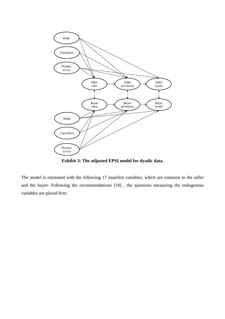
Exhibit 3: The adjusted EPSI model for dyadic data.
The model is estimated with the following 17 manifest variables, which are common to the seller
and the buyer. Following the recommendations [10] , the questions measuring the endogenous
variables are placed first:
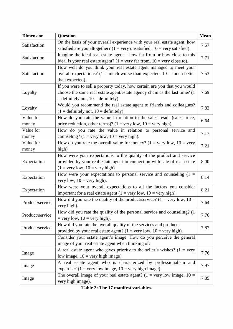
Dimension Question Mean
Satisfaction On the basis of your overall experience with your real estate agent, how
satisfied are you altogether? (1 = very unsatisfied, 10 = very satisfied). 7.57
Satisfaction Imagine the ideal real estate agent – how far from or how close to this
ideal is your real estate agent? (1 = very far from, 10 = very close to). 7.71
Satisfaction
How well do you think your real estate agent managed to meet your
overall expectations? (1 = much worse than expected, 10 = much better
than expected).
7.53
Loyalty
If you were to sell a property today, how certain are you that you would
choose the same real estate agent/estate agency chain as the last time? (1
= definitely not, 10 = definitely).
7.69
Loyalty Would you recommend the real estate agent to friends and colleagues?
(1 = definitely not, 10 = definitely). 7.83
Value for
money
How do you rate the value in relation to the sales result (sales price,
price reduction, other terms)? (1 = very low, 10 = very high). 6.64
Value for
money
How do you rate the value in relation to personal service and
counseling? (1 = very low, 10 = very high). 7.17
Value for
money
How do you rate the overall value for money? (1 = very low, 10 = very
high). 7.21
Expectation
How were your expectations to the quality of the product and service
provided by your real estate agent in connection with sale of real estate
(1 = very low, 10 = very high).
8.00
Expectation How were your expectations to personal service and counseling (1 =
very low, 10 = very high). 8.14
Expectation How were your overall expectations to all the factors you consider
important for a real estate agent (1 = very low, 10 = very high). 8.21
Product/service How did you rate the quality of the product/service? (1 = very low, 10 =
very high). 7.64
Product/service How did you rate the quality of the personal service and counseling? (1
= very low, 10 = very high). 7.76
Product/service How did you rate the overall quality of the services and products
provided by your real estate agent? (1 = very low, 10 = very high). 7.87
Consider your estate agent’s image. How do you perceive the general
image of your real estate agent when thinking of:
Image A real estate agent who gives priority to the seller’s wishes? (1 = very
low image, 10 = very high image). 7.76
Image A real estate agent who is characterized by professionalism and
expertise? (1 = very low image, 10 = very high image). 7.97
Image The overall image of your real estate agent? (1 = very low image, 10 =
very high image). 7.85
Table 2: The 17 manifest variables.

In June/July 2014, the questionnaire will be sent to 300 buyer/seller pairs who all within the last
three months have bought/sold real estate through DanBolig, one of the largest real estate chains in
Denmark.
In Denmark, a seller typically contacts one real estate agent who is commissioned to sell the
property. Potential buyers are then to contact this agent directly in order to see and possibly buy the
property. Accordingly, only one real estate agent is on commission to sell the property, and only the
seller pays for the service of the real estate agent – for the buyer, the service is free. Even though
the real estate agent, as a rule, is the seller’s agent, he must also take measures to satisfy the buyer
to ensure that he is in commission to resell the property in the future. In addition, most real estate
agents in Denmark are organized in real estate chains, so even if the sellers move away from the
area, a high level of satisfaction will, if nothing else, lead to a sense of loyalty towards the chain.
Finally, in all probability, the seller will share his experiences and level of estate agent satisfaction
with his former neighbors and additional social network connections in his old neighborhood.
Concluding remarks
In this paper, we have taken the first steps towards an EPSI model that can be used in businesses
where we, in the minefield between two types of customers, have a broker with the task to make
both ends meet. The model will be exposed to an empirical study in the summer of 2014. The idea
is to end up with a model that can be used when dealing with property – not only in the household
sector but also in the commercial real estate sector.
It would be really interesting to see if the estimated connections are the same in other parts of the
world, where the sale of property is organized in other ways (listings, two brokers etc.).
Furthermore, the approach described in this paper could also be relevant in other sectors that
operate as brokers between buyers and sellers. Examples of such sectors could be auction houses
and the transport sector.

References
[1] Fornell, C. 1992: “A National Customer Satisfaction Barometer: The Swedish Experience”,
Journal of Marketing, 56 (January), pp. 6-21, 1992.
[2] Juhl, H.J. et al, 2002: “Customer satisfaction in European food retailing”, Journal of Retailing
and Consumer Services 9 (2002) pp. 327-334.
[3] Kristensen, Kai, Martensen, A. & Grønholdt, L., 2000: “Customer satisfaction measurement
at Post Denmark: Results of application of the European Customer Satisfaction Index
Methodology”, Total Quality Management, 11, pp. 1007-1015, 2000.
[4] Eskildsen, J.K., Kristensen, 2008: “Customer satisfaction and customer loyalty as predictors
of future business potential”, Total Quality Management, 19(7-8), 2008, pp. 843-853.
[5] Kristensen, Kai, Martensen, A. & Grønholdt, L., 2002: “Customer satisfaction and business
performance” Neely(Ed): Business Performance Measurement – Theory and Practice, pp.
279-294 (Cambridge: Cambridge University Press).
[6] Kristensen, K., Eskildsen, J., 2005: “PLS structural equation modeling for customer
satisfaction measurement: Some empirical and theoretical results”. In F.W.Bliemel, A.Eggert,
G.Fassott, & J.Henseler (Eds), Handbuch PLS-Pfadmodellierung-Methode, Praxisbeispiele,
pp. 117-134, Schäffer-Poeschel.
[7] Wold, H. (1980). “Model construction and evaluation when theoretical knowledge is scarce:
Theory and application of Partial Least Squares”. In: J. Kmenta and J. B. Ramsey (Ed.),
Evaluation of Econometric Models, pp. 47-74, Academic Press, New York.
[8] Wold, H. (1985). “Partial Least Squares”. In: S. Kotz and N. Johnson (Ed.), Encyclopedia of
Statistical Sciences, pp. 581-591, Wiley, New York.
[9] Tenenhaus, M., Vinzi, V. V., Chatelin Y.-M. & Lauro, C. “PLS Path Modeling”,
Computational Statistics and Data Analysis, Jan 2005, 48, Issue 1, p. 159-205.
[10] Kristensen, K., Eskildsen, J., 2009: “Design of PLS-satisfaction studies, In Handbook of
Partial Least Squares: Concepts, Methods and Applications in Marketing and Relates fields,

Springer Handbooks of Computational Statistics, eds. V.E.Vinzi, W.W.Chin, J.Henseler and
H.Wang: Springer Verlag.
[11] Vinzi, V.E., Trinchera, L., Amato, S. 2010: PLS Path Modelling: From Foundations to Recent
Developments and Open Issues for Model Assessment and Improvement, In Handbook of
Partial Least Squares: Concepts, Methods and Applications in Marketing and Relates fields,
Springer Handbooks of Computational Statistics, eds. V.E.Vinzi, W.W.Chin, J.Henseler and
H.Wang: Springer Verlag.

EPSI Measurement on Dual Businesses
John Vestergaard Olesen
ICOA, BTECH, Aarhus University,
Birk Centerpark 15, 7400 Herning
Keywords: Market research methodology, PLS, satisfaction, EPSI, buyer-seller duality, simulation
study.
Abstract: This paper focuses on the design of a PLS structural equation model that can be used in
satisfaction studies in businesses that operate with a “buyer” and a “seller” on each side of an agent
– that is, in businesses where the satisfaction and loyalty become multidimensional at the latent
level. The traditional EPSI model is adjusted, and a complex model with six exogenous and six
endogenous variables is proposed. The model is exposed to a simulation study which investigates
the effect of the following factors: sample size, number of manifest variables and standard deviation
on the error terms in the measurement model.
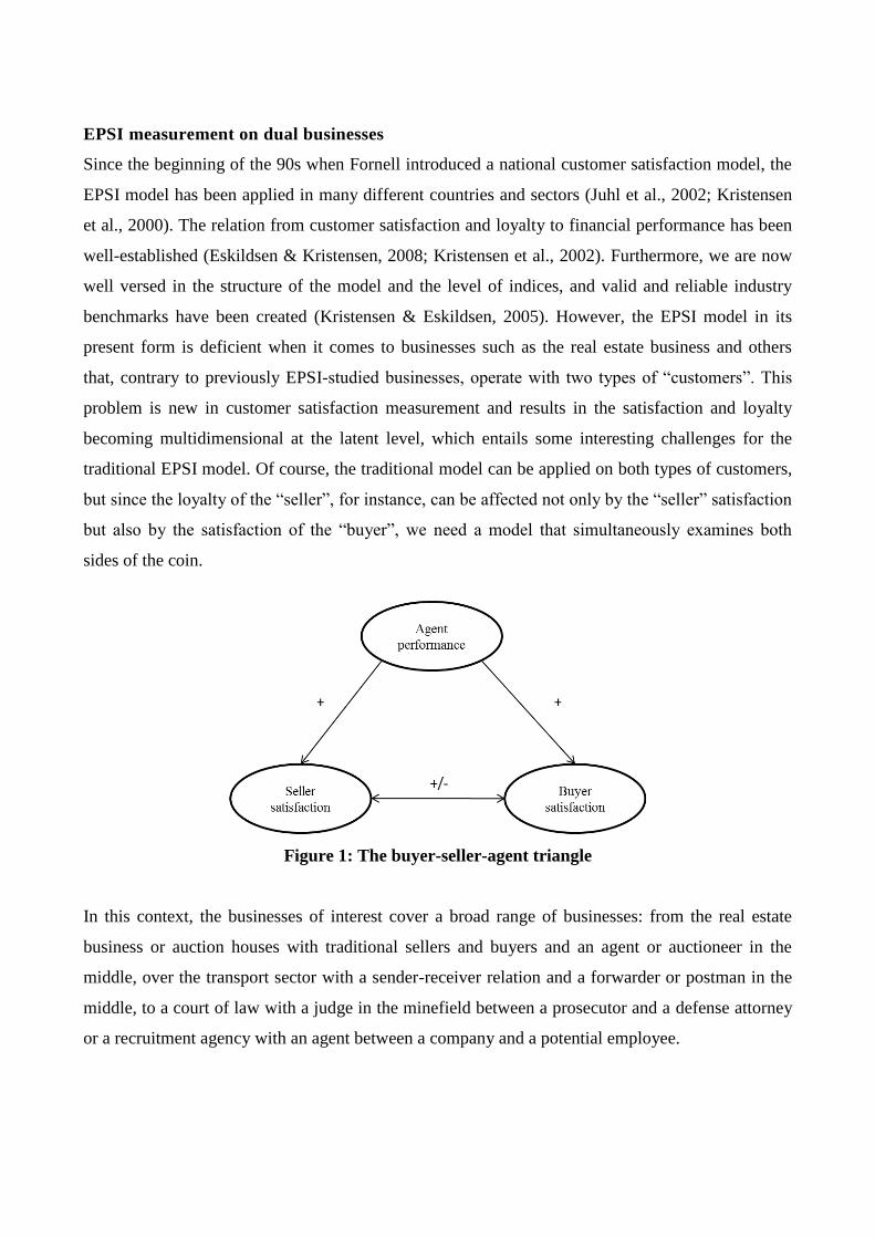
EPSI measurement on dual businesses
Since the beginning of the 90s when Fornell introduced a national customer satisfaction model, the
EPSI model has been applied in many different countries and sectors (Juhl et al., 2002; Kristensen
et al., 2000). The relation from customer satisfaction and loyalty to financial performance has been
well-established (Eskildsen & Kristensen, 2008; Kristensen et al., 2002). Furthermore, we are now
well versed in the structure of the model and the level of indices, and valid and reliable industry
benchmarks have been created (Kristensen & Eskildsen, 2005). However, the EPSI model in its
present form is deficient when it comes to businesses such as the real estate business and others
that, contrary to previously EPSI-studied businesses, operate with two types of “customers”. This
problem is new in customer satisfaction measurement and results in the satisfaction and loyalty
becoming multidimensional at the latent level, which entails some interesting challenges for the
traditional EPSI model. Of course, the traditional model can be applied on both types of customers,
but since the loyalty of the “seller”, for instance, can be affected not only by the “seller” satisfaction
but also by the satisfaction of the “buyer”, we need a model that simultaneously examines both
sides of the coin.
Figure 1: The buyer-seller-agent triangle
In this context, the businesses of interest cover a broad range of businesses: from the real estate
business or auction houses with traditional sellers and buyers and an agent or auctioneer in the
middle, over the transport sector with a sender-receiver relation and a forwarder or postman in the
middle, to a court of law with a judge in the minefield between a prosecutor and a defense attorney
or a recruitment agency with an agent between a company and a potential employee.

Though the mentioned businesses have the characteristic in common that both sides not necessarily
participate in paying for the product/service, the agent/auctioneer/postman/judge must take
measures to satisfy both parties. In Denmark, a seller typically contacts one real estate agent who is
commissioned to sell the property. Potential buyers are then to contact this agent directly in order to
see and possibly buy the property. Accordingly, only one real estate agent is on commission to sell
the property, and only the seller pays for the service of the real estate agent – for the buyer, the
service is free. Even though the real estate agent, as a rule, is the seller’s agent, he must also take
measures to satisfy the buyer to ensure that he is in commission to resell the property in the future.
In addition, most real estate agents in Denmark are organized in real estate chains, so even if the
sellers move away from the area, a high level of satisfaction will, if nothing else, lead to a sense of
loyalty towards the chain. Finally, in all probability, the seller will share his experiences and level
of estate agent satisfaction with his former neighbors and additional social network connections in
his old neighborhood.
Accordingly, the real estate agent faces the challenge of being able to simultaneously secure a high
satisfaction level among both the buyer and the seller. In this article, we will use terminology from
the real estate business and accordingly refer to the involved persons as agent, buyer, and seller,
respectively.
We introduce an adjusted EPSI model that can be applied to these dyadic cases, and the model will
be exposed to a simulation study in which we investigate the extent to which we, by the aid of the
simulated data, can reproduce the path coefficients we started with. PLS path modeling (Wold,
2008; Wold, 1985; Tenenhaus et al., 2005) will be applied to estimate the suggested relationships.
The article will conclude with recommendations for practitioners.
Analysis of dyadic data
In the presence of dyadic data, one of the key assumptions in many analyses, namely the
assumption of independency, is violated and needs to be addressed. Instead of seeing the violation
of this assumption as a problem that needs to be neglected or bypassed by only choosing either the
seller or the buyer, the point is that a study of both members of the dyad and addressing the
covariance across seller and buyer in the analysis of these non-interchangeable interdependent data
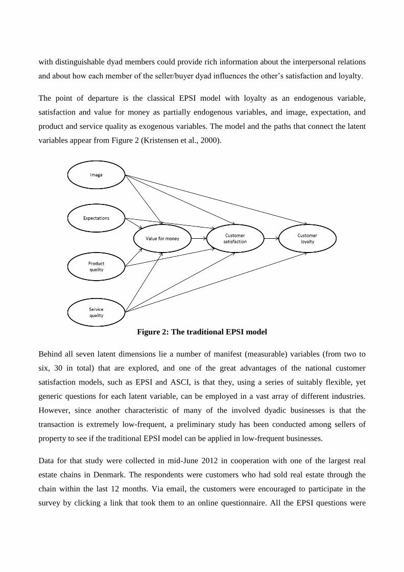
with distinguishable dyad members could provide rich information about the interpersonal relations
and about how each member of the seller/buyer dyad influences the other’s satisfaction and loyalty.
The point of departure is the classical EPSI model with loyalty as an endogenous variable,
satisfaction and value for money as partially endogenous variables, and image, expectation, and
product and service quality as exogenous variables. The model and the paths that connect the latent
variables appear from Figure 2 (Kristensen et al., 2000).
Figure 2: The traditional EPSI model
Behind all seven latent dimensions lie a number of manifest (measurable) variables (from two to
six, 30 in total) that are explored, and one of the great advantages of the national customer
satisfaction models, such as EPSI and ASCI, is that they, using a series of suitably flexible, yet
generic questions for each latent variable, can be employed in a vast array of different industries.
However, since another characteristic of many of the involved dyadic businesses is that the
transaction is extremely low-frequent, a preliminary study has been conducted among sellers of
property to see if the traditional EPSI model can be applied in low-frequent businesses.
Data for that study were collected in mid-June 2012 in cooperation with one of the largest real
estate chains in Denmark. The respondents were customers who had sold real estate through the
chain within the last 12 months. Via email, the customers were encouraged to participate in the
survey by clicking a link that took them to an online questionnaire. All the EPSI questions were
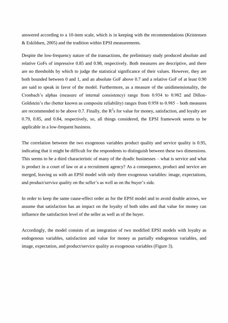
answered according to a 10-item scale, which is in keeping with the recommendations (Kristensen
& Eskildsen, 2005) and the tradition within EPSI measurements.
Despite the low-frequency nature of the transactions, the preliminary study produced absolute and
relative GoFs of impressive 0.85 and 0.98, respectively. Both measures are descriptive, and there
are no thresholds by which to judge the statistical significance of their values. However, they are
both bounded between 0 and 1, and an absolute GoF above 0.7 and a relative GoF of at least 0.90
are said to speak in favor of the model. Furthermore, as a measure of the unidimensionality, the
Cronbach’s alphas (measure of internal consistency) range from 0.934 to 0.982 and Dillon-
Goldstein’s rho (better known as composite reliability) ranges from 0.958 to 0.985 – both measures
are recommended to be above 0.7. Finally, the R2s for value for money, satisfaction, and loyalty are
0.79, 0.85, and 0.84, respectively, so, all things considered, the EPSI framework seems to be
applicable in a low-frequent business.
The correlation between the two exogenous variables product quality and service quality is 0.95,
indicating that it might be difficult for the respondents to distinguish between these two dimensions.
This seems to be a third characteristic of many of the dyadic businesses – what is service and what
is product in a court of law or at a recruitment agency? As a consequence, product and service are
merged, leaving us with an EPSI model with only three exogenous variables: image, expectations,
and product/service quality on the seller’s as well as on the buyer’s side.
In order to keep the same cause-effect order as for the EPSI model and to avoid double arrows, we
assume that satisfaction has an impact on the loyalty of both sides and that value for money can
influence the satisfaction level of the seller as well as of the buyer.
Accordingly, the model consists of an integration of two modified EPSI models with loyalty as
endogenous variables, satisfaction and value for money as partially endogenous variables, and
image, expectation, and product/service quality as exogenous variables (Figure 3).
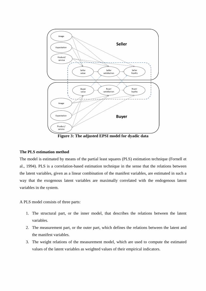
Figure 3: The adjusted EPSI model for dyadic data
The PLS estimation method
The model is estimated by means of the partial least squares (PLS) estimation technique (Fornell et
al., 1994). PLS is a correlation-based estimation technique in the sense that the relations between
the latent variables, given as a linear combination of the manifest variables, are estimated in such a
way that the exogenous latent variables are maximally correlated with the endogenous latent
variables in the system.
A PLS model consists of three parts:
1. The structural part, or the inner model, that describes the relations between the latent
variables.
2. The measurement part, or the outer part, which defines the relations between the latent and
the manifest variables.
3. The weight relations of the measurement model, which are used to compute the estimated
values of the latent variables as weighted values of their empirical indicators.

If the vector of endogenous variables and the associated coefficient matrix is denoted with η⃗ and B,
respectively, and ξ is a vector of the latent exogenous variables with an associated coefficient
matrix Γ, the relation is given by the matrix equation
�⃗⃗� = 𝚩�⃗⃗� + 𝚪𝛏 + 𝛇
where ζ⃗⃗ is a residual vector of which we will assume the usual properties (zero mean,
homoscedasticity and zero covariance between the errors).
If m and k are the number of endogenous and exogenous latent variables, respectively, the m-
dimensional vector �⃗⃗� and the k-dimensional vector �⃗� look as follows:
�⃗⃗� =
(
𝜂1: 𝑉𝑎𝑙𝑢𝑒 𝑓𝑜𝑟 𝑚𝑜𝑛𝑒𝑦, 𝑠𝑒𝑙𝑙𝑒𝑟𝜂2: 𝑆𝑒𝑙𝑙𝑒𝑟 𝑠𝑎𝑡𝑖𝑠𝑓𝑎𝑐𝑡𝑖𝑜𝑛 𝜂3: 𝑆𝑒𝑙𝑙𝑒𝑟 𝑙𝑜𝑦𝑎𝑙𝑡𝑦 𝜂4: 𝑉𝑎𝑙𝑢𝑒 𝑓𝑜𝑟 𝑚𝑜𝑛𝑒𝑦, 𝑏𝑢𝑦𝑒𝑟𝜂5: 𝐵𝑢𝑦𝑒𝑟 𝑠𝑎𝑡𝑖𝑠𝑓𝑎𝑐𝑡𝑖𝑜𝑛 𝜂6: 𝐵𝑢𝑦𝑒𝑟 𝑙𝑜𝑦𝑎𝑙𝑡𝑦 )
and
�⃗� =
(
𝜉1: 𝐼𝑚𝑎𝑔𝑒, 𝑠𝑒𝑙𝑙𝑒𝑟 𝜉2: 𝐸𝑥𝑝𝑒𝑐𝑡𝑎𝑡𝑖𝑜𝑛, 𝑠𝑒𝑙𝑙𝑒𝑟 𝜉3: 𝑃𝑟𝑜𝑑𝑢𝑐𝑡 𝑎𝑛𝑑 𝑠𝑒𝑟𝑣𝑖𝑐𝑒 𝑞𝑢𝑎𝑙𝑖𝑡𝑦, 𝑠𝑒𝑙𝑙𝑒𝑟 𝜉4: 𝐼𝑚𝑎𝑔𝑒, 𝑏𝑢𝑦𝑒𝑟 𝜉5: 𝐸𝑥𝑝𝑒𝑐𝑡𝑎𝑡𝑖𝑜𝑛, 𝑏𝑢𝑦𝑒𝑟 𝜉6: 𝑃𝑟𝑜𝑑𝑢𝑐𝑡 𝑎𝑛𝑑 𝑠𝑒𝑟𝑣𝑖𝑐𝑒 𝑞𝑢𝑎𝑙𝑖𝑡𝑦, 𝑏𝑢𝑦𝑒𝑟)
With the opposed relations between the endogenous variables and the traditional relations between
the exogenous and endogenous variables, the m x m-dimensional coefficient matrix B and the m x
k-dimensional coefficient matrix 𝚪 giving the inner structure will therefore be
𝐁 =
(
0 0 0 0 0 0𝛽21 0 0 𝛽24 0 00 𝛽32 0 0 𝛽35 00 0 0 0 0 0𝛽51 0 0 𝛽54 0 00 𝛽62 0 0 𝛽65 0)
and 𝚪 =
(
𝛾11 𝛾12 𝛾13 0 0 0𝛾21 𝛾22 𝛾23 0 0 0𝛾31 0 𝛾33 0 0 00 0 0 𝛾44 𝛾45 𝛾460 0 0 𝛾54 𝛾55 𝛾560 0 0 𝛾64 0 𝛾66)
,

where 𝛽𝑖𝑗 is the path coefficient that goes from endogenous variable j to endogenous variable i, and
𝛾𝑖𝑗 is the path coefficient that combines exogenous variable j to endogenous variable i (Figure 4).
Figure 4: The adjusted EPSI model for dual measurements
The second part of the PLS model is the measurement model, and in PLS, these outer relations can
be reflective as well as formative (Jöreskog et al., 1982). If �⃗� and 𝐲 are vectors of the observed 𝛏
and �⃗⃗� indicators with error vectors 𝛅𝐱⃗⃗⃗⃗ and 𝛜𝐲⃗⃗ ⃗, respectively, and Λx and Λy are the matrices that
contain the λi coefficients (loadings) combining the latent and manifest variables for the exogenous
and endogenous variables, respectively, the general equations for reflective external relations are
𝐲 = 𝚲𝐲�⃗⃗� + 𝛆𝐲⃗⃗ ⃗

�⃗� = 𝚲𝐱𝛏 + 𝛅𝐱⃗⃗⃗⃗
If we let 𝐲 𝐢′ = (𝑦𝑖1, 𝑦𝑖2, … , 𝑦𝑖𝐻𝑖) be the vector of manifest variables related to the latent endogenous
variable ηi and �⃗� 𝐢′ = (𝑥𝑖1, 𝑥𝑖2, … , 𝑥𝑖𝐺𝑖) be the vector of manifest variables related to the latent
exogenous variableξi, the measurement model can be written as
yij = λyijηi + ϵij, i = 1, … , 6; j = 1, … , Hi
xij = λxijξi + δij, i = 1,… , 6; j = 1,… , Gi
where Hi and Gi are the number of manifest variables associated with the latent variables ηi and ξi,
respectively.
In the weight relations – the final part of the PLS model – the estimated values of the latent
variables are given as linear sums of the empirical indicators:
η̂i = ∑ωijyij ,
Hi
j=1
i = 1,… ,6
ξ̂i = ∑ωijxij ,
Gi
j=1
i = 1,… ,6
The estimation of the PLS model now consists of the following three steps:
1. Estimate the weight relations of the measurement model via the PLS algorithm.
2. Estimate the values of latent variables based on the weights from step 1.
3. Estimate the structural parameters based on the latent variable values estimated in step 2.
Data generating process
In the data generating process of the suggested model, we assume that the coefficients of the
structural model are known. The postulated structural model is thus given by the matrices

𝐁 =
(
0 0 0 0 0 0𝛽21 0 0 𝛽24 0 00 𝛽32 0 0 𝛽35 00 0 0 0 0 0𝛽51 0 0 𝛽54 0 00 𝛽62 0 0 𝛽65 0)
=
(
0 0 0 0 0 00.11 0 0 0.30 0 00 0.77 0 0 0.50 00 0 0 0 0 00.30 0 0 0.11 0 00 0.50 0 0 0.77 0)
and
𝚪 =
(
𝛾11 𝛾12 𝛾13 0 0 0𝛾21 𝛾22 𝛾23 0 0 0𝛾31 0 𝛾33 0 0 00 0 0 𝛾44 𝛾45 𝛾460 0 0 𝛾54 𝛾55 𝛾560 0 0 𝛾64 0 𝛾66)
=
(
0.22 −0.15 0.80 0 0 00.28 −0.17 0.73 0 0 00.13 0 0.26 0 0 00 0 0 0.22 −0.15 0.800 0 0 0.28 −0.17 0.730 0 0 0.13 0 0.26)
implying that the equations for the investigated model without the residuals for the seller is given by
the equations
𝜂𝑉𝑎𝑙𝑢𝑒𝑆𝑒𝑙𝑙𝑒𝑟 = 0.22 ∙ 𝜉𝐼𝑚𝑎𝑔𝑒
𝑆𝑒𝑙𝑙𝑒𝑟 − 0.15 ∙ 𝜉𝐸𝑥𝑝𝑒𝑐𝑡𝑎𝑡𝑖𝑜𝑛𝑆𝑒𝑙𝑙𝑒𝑟 + 0.80 ∙ 𝜉𝑃𝑟𝑜𝑑𝑢𝑐𝑡/𝑆𝑒𝑟𝑣𝑖𝑐𝑒
𝑆𝑒𝑙𝑙𝑒𝑟
𝜂𝑆𝑎𝑡𝑖𝑠𝑓𝑎𝑐𝑡𝑖𝑜𝑛𝑆𝑒𝑙𝑙𝑒𝑟 = 0.28 ∙ 𝜉𝐼𝑚𝑎𝑔𝑒
𝑆𝑒𝑙𝑙𝑒𝑟 − 0.17 ∙ 𝜉𝐸𝑥𝑝𝑒𝑐𝑡𝑎𝑡𝑖𝑜𝑛𝑆𝑒𝑙𝑙𝑒𝑟 + 0.73 ∙ 𝜉𝑃𝑟𝑜𝑑𝑢𝑐𝑡/𝑆𝑒𝑟𝑣𝑖𝑐𝑒
𝑆𝑒𝑙𝑙𝑒𝑟 + 0.11 ∙ 𝜂𝑉𝑎𝑙𝑢𝑒𝑆𝑒𝑙𝑙𝑒𝑟 + 0.3 ∙ 𝜂𝑉𝑎𝑙𝑢𝑒
𝐵𝑢𝑦𝑒𝑟
𝜂𝐿𝑜𝑦𝑎𝑙𝑡𝑦𝑆𝑒𝑙𝑙𝑒𝑟 = 0.13 ∙ 𝜉𝐼𝑚𝑎𝑔𝑒
𝑆𝑒𝑙𝑙𝑒𝑟 + 0.26 ∙ 𝜉𝑃𝑟𝑜𝑑𝑢𝑐𝑡/𝑆𝑒𝑟𝑣𝑖𝑐𝑒𝑆𝑒𝑙𝑙𝑒𝑟 + 0.77 ∙ 𝜂𝑆𝑎𝑡𝑖𝑠𝑓𝑎𝑐𝑡𝑖𝑜𝑛
𝑆𝑒𝑙𝑙𝑒𝑟 + 0.5 ∙ 𝜂𝑆𝑎𝑡𝑖𝑠𝑓𝑎𝑐𝑡𝑖𝑜𝑛𝐵𝑢𝑦𝑒𝑟
The relations for the buyer are given by corresponding equations.
These values are chosen to make the path coefficients within the two EPSI models identical and in
alignment with the values from the preliminary study. Furthermore, these coefficients do not differ
much from what we usually see in EPSI measurements. In addition, the path coefficients that
combine the buyer and seller parts are chosen so that 𝛽24 = 𝛽51 = 0.30 and 𝛽35 = 𝛽62 = 0.50,
making the model symmetrical. Since this problem is new in EPSI measurements, these parameters
are unknown and have never been estimated. The values are chosen randomly, and there are
arguments in favor of both signs.

Simulation results
In the simulation study, we focus on the three factors of sample size, number of manifest variables,
and standard deviation on the error terms in the measurement model as well as the following levels:
Number of manifest indicators: p = [2; 4; 6].
Standard deviation on the error terms in the measurement model: 𝜎𝜀= [1; 5; 10; 20].
Sample size: n = [50; 100; 250; 1000].
Therefore, we completed a full factorial design with three factors in 3 ∙ 4 ∙ 4 = 48 runs, giving a
total of 16.800 “pairs of respondents” and a total of 806.400 values of manifest variables.
To evaluate the consequences of the consistency at large concept, we included the number of
manifest variables per latent variable as a factor in the simulation study. The path coefficients going
from the exogenous variables to the endogenous variables are called the 1st generation, while the
four path coefficients from value to satisfaction and the four from satisfaction to loyalty are called
2nd and 3rd generation, respectively. In Error! Reference source not found., the impact that the
number of manifest indicators per latent variable has on the mean absolute bias is shown. As it
appears, the pattern in all three generations is that the bias decreases as the number of manifest
indicators increases, thus lending support to the consistency at large concept. From Figure 6, we
also see that the degree of explanations for value for money, satisfaction, and loyalty increases as
the number of indicators increases.

Figure 5: Mean absolute bias of the path coefficients:
The effect of the number of manifest indicators
Figure 6: Degree of explanations of the three levels of endogenous variables:
The effect of the number of manifest indicators
0
0,05
0,1
0,15
0,2
0,25
0 2 4 6 8
Mea
n a
bso
lute
bia
s
Number of indicators
1st generation
2nd generation
3rd generation
0,8
0,85
0,9
0,95
1
0 2 4 6 8
R2
Number of indicators
Value for money
Satisfaction
Loyalty
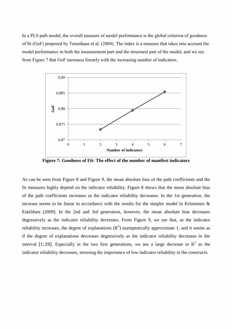
In a PLS path model, the overall measure of model performance is the global criterion of goodness
of fit (GoF) proposed by Tenenhaus et al. (2004). The index is a measure that takes into account the
model performance in both the measurement part and the structural part of the model, and we see
from Figure 7 that GoF increases linearly with the increasing number of indicators.
Figure 7: Goodness of Fit: The effect of the number of manifest indicators
As can be seen from Figure 8 and Figure 9, the mean absolute bias of the path coefficients and the
fit measures highly depend on the indicator reliability. Figure 8 shows that the mean absolute bias
of the path coefficients increases as the indicator reliability decreases. In the 1st generation, the
increase seems to be linear in accordance with the results for the simpler model in Kristensen &
Eskildsen (2009). In the 2nd and 3rd generation, however, the mean absolute bias decreases
degressively as the indicator reliability decreases. From Figure 9, we see that, as the indicator
reliability increases, the degree of explanations (R2) asymptotically approximate 1, and it seems as
if the degree of explanations decreases degressively as the indicator reliability decreases in the
interval [1; 20]. Especially in the two first generations, we see a large decrease in R2 as the
indicator reliability decreases, stressing the importance of low indicator reliability in the constructs.
0,87
0,875
0,88
0,885
0,89
0 1 2 3 4 5 6 7
Go
F
Number of indicators
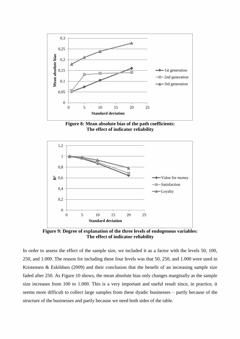
Figure 8: Mean absolute bias of the path coefficients:
The effect of indicator reliability
Figure 9: Degree of explanation of the three levels of endogenous variables:
The effect of indicator reliability
In order to assess the effect of the sample size, we included it as a factor with the levels 50, 100,
250, and 1.000. The reason for including these four levels was that 50, 250, and 1.000 were used in
Kristensen & Eskildsen (2009) and their conclusion that the benefit of an increasing sample size
faded after 250. As Figure 10 shows, the mean absolute bias only changes marginally as the sample
size increases from 100 to 1.000. This is a very important and useful result since, in practice, it
seems more difficult to collect large samples from these dyadic businesses – partly because of the
structure of the businesses and partly because we need both sides of the table.
0
0,05
0,1
0,15
0,2
0,25
0,3
0 5 10 15 20 25
Mea
n a
bso
lute
bia
s
Standard deviation
1st generation
2nd generation
3rd generation
0
0,2
0,4
0,6
0,8
1
1,2
0 5 10 15 20 25
R2
Standard deviation
Value for money
Satisfaction
Loyalty

Figure 10: Mean absolute bias of the path coefficients:
The effect of the sample size
Though the model in this simulation study is much more complex than the one used in Kristensen &
Eskildsen (2009), the fact that we see the decreasing effect on the absolute bias of the path
coefficients, also in the 1st generation, makes us draw the conclusion that a sample size of 100 is
sufficient for practitioners to ensure a reasonable level of bias of the path coefficients in a PLS
structural equation model in general. Indeed, Figure 11, which shows the degree of explanations in
the three types of endogenous variables as a function of the sample size, makes it very difficult to
argue for a sample size larger than 100.
0
0,05
0,1
0,15
0,2
0,25
0 200 400 600 800 1000 1200
Mea
n a
bso
lute
bia
s
Sample size
1st generation
2nd generation
3rd generation
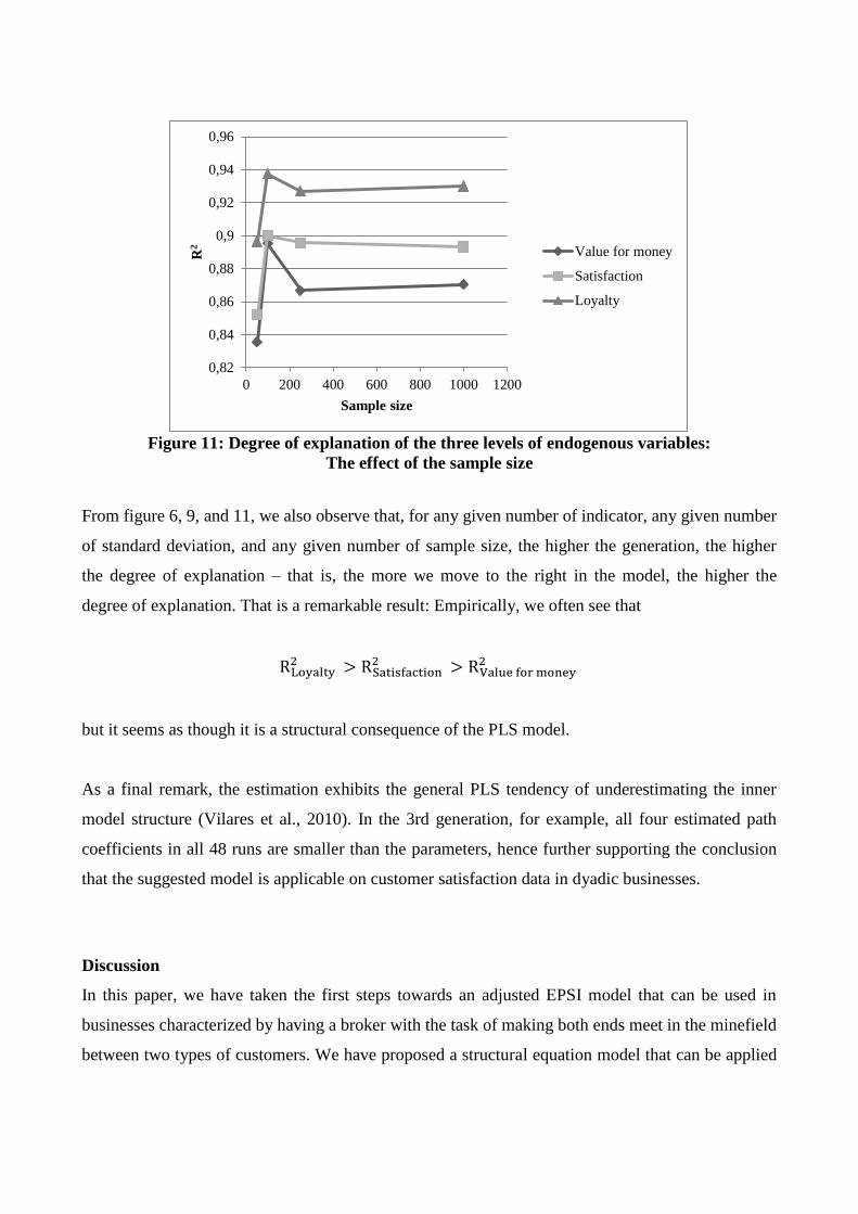
Figure 11: Degree of explanation of the three levels of endogenous variables:
The effect of the sample size
From figure 6, 9, and 11, we also observe that, for any given number of indicator, any given number
of standard deviation, and any given number of sample size, the higher the generation, the higher
the degree of explanation – that is, the more we move to the right in the model, the higher the
degree of explanation. That is a remarkable result: Empirically, we often see that
RLoyalty 2 > RSatisfaction
2 > RValue for money 2
but it seems as though it is a structural consequence of the PLS model.
As a final remark, the estimation exhibits the general PLS tendency of underestimating the inner
model structure (Vilares et al., 2010). In the 3rd generation, for example, all four estimated path
coefficients in all 48 runs are smaller than the parameters, hence further supporting the conclusion
that the suggested model is applicable on customer satisfaction data in dyadic businesses.
Discussion
In this paper, we have taken the first steps towards an adjusted EPSI model that can be used in
businesses characterized by having a broker with the task of making both ends meet in the minefield
between two types of customers. We have proposed a structural equation model that can be applied
0,82
0,84
0,86
0,88
0,9
0,92
0,94
0,96
0 200 400 600 800 1000 1200
R2
Sample size
Value for money
Satisfaction
Loyalty
to customer satisfaction data in these businesses where the satisfaction and loyalty dimensions are
multidimensional, and we have investigated the quality of PLS estimation when applied on
simulated data.
In the simulation study, we focused on the three factors of sample size, number of manifest
variables, and standard deviation on the error terms in the measurement model and the levels n =
[50; 100; 250; 1000], p = [2; 4; 6], and 𝜎𝜀= [1; 5; 10; 20], respectively. All in all, despite its high
complexity, the model roughly behaves as expected. Consistency at large and the importance of low
indicator reliability in the constructs are very conspicuous, stressing the significance for the
practitioners to formulate questions with as low a standard deviation as possible. In terms of the
sample size, the simulation study suggests that sample sizes of 100 are sufficient to ensure a
reasonable level of bias of the path coefficients in the model – a very useful result, partly since we
in some of the affected industries will struggle to find respondents, and partly since we need
“seller”-“buyer” pairs and not only a number of “buyers” and “sellers”.
Obviously, more work needs to be done: A limitation of this study is that we have not incorporated
different levels of skewness in the simulation, and research needs to be done on this. Also, we have
only investigated the ability to reproduce the inner model coefficients, and research should be
conducted to uncover the consequences for the predictions of the latent variables as well. However,
PLS is usually a useful tool in these predictions, so the fact that the model and the PLS estimation
technique work fine in reproducing the path coefficients, where covariance-based techniques
traditionally have the upper hand, seems promising. Additionally, the longer we move to the right in
the suggested model, the more multicollinearity becomes a problem; however, the fact that the
model behaved nicely in the 1st generation indicates that it also might work well with an adjusted
EPSI model where we do not merge the product and service construct and instead have a model
with 2*4 exogenous variables and 2*3 endogenous variables. For businesses where it is easy to
distinguish between product and service, this might prove important. Finally, the model needs to be
exposed to real-world data. In a coming study within the real estate business, the behavior of the
model will be further examined. Especially the relations between the endogenous variables will be
put under the microscope.
References
Eskildsen, J.K., Kristensen, 2008: “Customer satisfaction and customer loyalty as predictors of
future business potential”, Total Quality Management, 19(7-8), 2008, pp. 843-853.
Fornell, C. 1992: “A National Customer Satisfaction Barometer: The Swedish Experience”, Journal
of Marketing, 56 (January), pp. 6-21, 1992.
Juhl, H.J. et al, 2002: “Customer satisfaction in European food retailing”, Journal of Retailing and
Consumer Services 9 (2002) pp. 327-334.
Kristensen, Kai, Martensen, A. & Grønholdt, L., 2000: “Customer satisfaction measurement at Post
Denmark: Results of application of the European Customer Satisfaction Index Methodology”, Total
Quality Management, 11, pp. 1007-1015, 2000.
Kristensen, K., Eskildsen, J., 2005: “PLS structural equation modeling for customer satisfaction
measurement: Some empirical and theoretical results”. In F.W.Bliemel, A.Eggert, G.Fassott, &
J.Henseler (Eds), Handbuch PLS-Pfadmodellierung-Methode, Praxisbeispiele, pp. 117-134,
Schäffer-Poeschel.
Kristensen, K., Eskildsen, J., 2009: “Design of PLS-satisfaction studies, In Handbook of Partial
Least Squares: Concepts, Methods and Applications in Marketing and Relates fields, Springer
Handbooks of Computational Statistics, eds. V.E.Vinzi, W.W.Chin, J.Henseler and H.Wang:
Springer Verlag.
Kristensen, Kai, Martensen, A. & Grønholdt, L., 2002: ”Customer satisfaction and business
performance” Neely(Ed): Business Performance Measurement – Theory and Practice, pp. 279-294
(Cambridge: Cambridge University Press).
Tenenhaus, M., Vinzi, V. V., Chatelin, Y. M. & Lauro, C. "PLS Path Modeling", Computational
Statistics and Data Analysis, Jan 2005, 48, Issue 1, p. 159-205.
Tenenhaus, M., Amato, S., and Esposito Vinzi, V. (2004): A Global goodness-of-fit index for PLS
structural equation modeling. Proceedings of the XLII SIS Scientific Meeting, Vol. Contributed
Papers, CLEUP, Padova, pp. 739-742.
Vilares, M. J., Almeida, M. H., and Coelho, P.S. (2010): Comparison of Likelihood and PLS
Estimators for Structural Equation Modeling: A simulation with Customer Satisfaction Data. In
Handbook of Partial Least Squares: Concepts, Methods and Applications in Marketing and Relates
fields, Springer Handbooks of Computational Statistics, eds. V.E.Vinzi, W.W.Chin, J.Henseler and
H.Wang: Springer Verlag.
Vinzi, V.E., Trinchera, L., Amato, S. 2010: PLS Path Modelling: From Foundations to Recent
Developments and Open Issues for Model Assessment and Improvement, In Handbook of Partial
Least Squares: Concepts, Methods and Applications in Marketing and Relates fields, Springer
Handbooks of Computational Statistics, eds. V.E.Vinzi, W.W.Chin, J.Henseler and H.Wang:
Springer Verlag.
Wold, H. (1980). "Model construction and evaluation when theoretical knowledge is scarce: Theory
and application of Partial Least Squares". In: J. Kmenta and J. B. Ramsey (Ed.), Evaluation of
Econometric Models, pp. 47-74, Academic Press, New York.
Wold, H. (1985). "Partial Least Squares". In: S. Kotz and N. Johnson (Ed.), Encyclopedia of
Statistical Sciences, pp. 581-591, Wiley, New York.