measurements of extreme waves

Measurements of Extreme Waves!

Jim Thomson Northwest Na0onal Marine Renewable Energy Center

Applied Physics Lab University of Washington

“Extreme Waves”

•  Individual waves: rogue waves (H > 2.2 Hs) – nonlinearity, non Gaussian sta0s0cs

•  refrac0ve focusing (currents, bathymetry) •  crossing seas (direc0onality)

•  Individual waves: unexpected waves (Hi > 2 Hj) –  intermiRence within Gaussian sta0s0cs, groups

•  High sea states: storms and hurricanes – wave steepness, breaking –  importance of wind forcing

Wave measurements: buoys, pressure gages, sonar al0meters, lidar, radar,

Limita&ons of in situ point measurements: •  localized in space, short in dura&on (usually) •  only first five spectral moments Limita&ons of remote sensing (e.g. radar): •  Calibra&on •  Resolu&on

Nortek AWAC

APL SWIFT

cartoon

Datawell waverider

Example: 14 m waves at Sta0on P (Ocean reference site with ongoing NSF-‐funded 0me series and wave dynamics studies… e.g., Thomson et al, JGR, 2013)

19 Dec 2012 at 17:00 UTC

Example: 14 m wave at Sta0on P Fully developed sea (P-‐M limit), gH / U2, g T/ U For the observed Hs = 14 m,

Theore0cal U10 = 20 m/s, Observed U4 = 18 m/s Theore0cal Tp = 19.5 s, Observed Tp = 18 s

The 14 m Hs is consistent with parametric spectra and wind forcing, but it is s0ll ‘extreme’ rela0ve to climatology

Climatology (Hs stats by month)

Example: 11 m waves at Sta0on P (Ocean reference site with ongoing NSF-‐funded 0me series and wave dynamics studies)

01 Nov 2010 at 00:30 UTC

Example: 11 m wave at Sta0on P Fully developed sea (P-‐M limit), gH / U2, g T/ U For the observed Hs = 11 m,

Theore0cal U10 = 18 m/s, Observed U4 = 14 m/s Theore0cal Tp = 17 s, Observed Tp = 18 s

Example: 11 m waves at Sta0on P

18 m peak-‐to-‐trough ( = 1.6 Hs)

Compare to raw (wave by wave) data, where 1800 s at Tp = 18 s is about 100 waves Rayleigh says 100 waves have H = 1.6 Hs, and 1000 waves have H = 2 Hs

Climatology (Hs stats by month)

The 11 m Hs is consistent with parametric spectra and wind forcing, AND THE RAW DATA IS CONSISTENT WITH RAYLEIGH, but it is s0ll ‘extreme’ rela0ve to climatology

Sta0on P overall Sta0on P stats (and extremes) from 4 yrs

Wave He

ight [m

]

Peak wave period, Tp [s]

N

Extremes (N < 1)

Tp [s]

H [m

]

0 5 10 15 20 250

2

4

6

8

10

12

14Hk = 0.88Hk = 0.44Hk = 0.22

Steepness curves

Extreme forces: wave breaking •  Steepness limits: Stokes: 1/7, Miche: •  Importance of groups à resonant nonlineari0es and

instabili0es (e.g. Benjamin-‐Feir) •  Par0cle speed exceeds phase speed à large forces, especially

iner0al… accelera&on goes as H ω2

(Hk)max

= 0.88 tanh(�kd

0.88)

changes. Large, vigorous whitecaps start to replace thesmall, transient breaking events seen at the shorterfetches, and evidence of microbreaking becomes lessapparent. These larger whitecaps (Fig. 4f) are more visi-ble from the shipboard video (Fig. 4d) and the breakingrates converge for later times.

The higher breaking rates from the SWIFT videoduring calmer conditions are consistent with the in situ

turbulent dissipation estimates. As shown in Fig. 9, bothbreaking and dissipation increase approximately oneorder of magnitude as waves evolve and steepen. Thisimplies that each wave dissipates roughly the sameamount of energy during breaking, such that morebreaking produces more dissipation. The breaking ratesfrom the shipboard video, by contrast, increase muchmore dramatically than the dissipation estimates, whichwould imply that each breaking wave contributes lessdissipation as the wave field evolves. This is both phys-ically unlikely and contrary to the Duncan–Phillipstheory, where the dissipation rate of a breaking wave isproportional to c5 times its crest length, with a proposedadditional positive dependence on wave slope (Melville1994; Drazen et al. 2008). Thus, only ship-based videorecordings from the rougher conditions (filled symbolsof Fig. 9a) are used in assessing the L(c) and b results.

d. Breaking strength parameter

The value of the bulk breaking parameter b is calcu-lated from

b 5Sds

rwg21

ðc5L(c) dc

, (22)

using each of the four measures of dissipation Sds fromFig. 8. These calculated b values are shown as a functionof mss, wave age, and significant steepness in Fig. 10. Onlyone SWIFT was in the water during the two 15 Februaryvideo segments; thus, there is one less b value for theseL(c). The independent variables use the average of mss,cp, U10, and Hs within a 500-m region around each L(c)calculation. As in Fig. 9a, values that are biased by in-sufficient pixel resolution are shown with open symbols.

In addition, data are included from measurementsmade in Lake Washington, in 2006 and Puget Sound, in2008, originally reported in Thomson et al. (2009).Whereas in Thomson et al. (2009) a constant b was ob-tained via regression of

Ðc5L(c) dc to the measured

dissipation, here individual values of b are calculated.Apart from the updates to the Fourier method detailedin the appendix, the L(c) methodology is similar be-tween the datasets. The comparison of b with wave ageand steepness is in part motivated by the desire tocompare across these datasets, as the spectra from theearlier measurements are of insufficient quality to cal-culate mean square slope.

As expected, the b values are affected by under-counting small whitecaps in less steep seas. The biasedpoints, shown in open symbols, have dramatic trends ofdecreasing b with increasing wind forcing (described byinverse wave age U10/cp) and increasing wave slope (using

FIG. 9. (a) Breaking rate and (b) wave dissipation vs mss. Circlescorrespond to shipboard measurements from 14 Feb and squaresare from shipboard measurements during 15 Feb in (a). Asterisksand crosses are from manual SWIFT breaking rate counts for14 and 15 Feb, respectively. Data plotted with open symbolsoverlap with the SWIFT breaking rates (in time) and appear tounderestimate the breaking rate. Wave dissipation from Fig. 8 isplotted vs mss for SWIFT 1 (red), SWIFT 2 (cyan), DopBeam (blue),and inferred dissipation from the RTE based on the stationary as-sumption (black) in (b).

JANUARY 2014 S C H W E N D E M A N E T A L . 117

Mean square slope

Breaking ra

te

10,000 lb rated line parted upon impact of 3 m breaker

Some recent literature

Oceanography | Vol.24, No.2160

elevation relative to the mean sea surface height and std is the standard devia-tion. Rogue waves are o!en thought to be extremely large and destructive, but because they are de"ned relative to the signi"cant wave height, the majority of the rogue waves are only a few meters high. While these waves may cause signi"cant damage to smaller vessels, the buoys also recorded 69 waves of more than 11 m in height. #e largest

rogue wave found in the data occurred at buoy 71 (Harvest, CA) on February 24, 2008, 21:19 UTC and is shown in Figure 2a. It is the second of two rogue waves immediately following each other. #e trough-to-crest heights of the two waves are 16.7 m and 18.95 m, the zero-crossing wave period is 15.5 s, and the H/Hs ratios are 2.4 and 2.3. #e magnitudes of the horizontal displacements are 23.0 m and 16.8 m.

Horizontal and vertical displacements indicate an approximately circular wave motion (Figure 2b). #e directions of the rogue waves agree with the hourly directional wave spectra provided by the Coastal Data Information Program within < 20° (Figure 2c).

ROGUE WAVE STATISTICS#e average number of rogue waves per year is calculated by comparing the number of rogue waves found at each buoy to its total “time on” and to the total number of waves. In a total of 80.8 years of data and 6.1 x 108 waves at all moorings, 7,157 rogue waves with a ratio of H/Hs ≥ 2.0 were observed, averaging 88.6 rogue waves per year, or about one in 84,500 waves (Table 2). For a ratio of H/Hs ≥ 2.2, a total of 687 rogue waves were counted, yielding an average of 8.5 rogue waves per year or one in 880,000 waves. #e maximum observed ratio of H/Hs was 2.57 for a 4.1-m-high wave at buoy 128. #e maximum rogue wave height was 18.95 m at buoy 71 (Figure 2).

#e statistics vary signi"cantly when open ocean, shallow water, and coastal ocean are considered separately (Table 2). While in the open ocean and shallow water, about 100 rogue waves of H/Hs ≥ 2.0 and 9 to 11 rogue waves of H/Hs ≥ 2.2 occur per year, they are less frequent in the protected coastal waters with 63 and 6 rogue waves per year for H/Hs ≥ 2.0 and H/Hs ≥ 2.2, respectively.

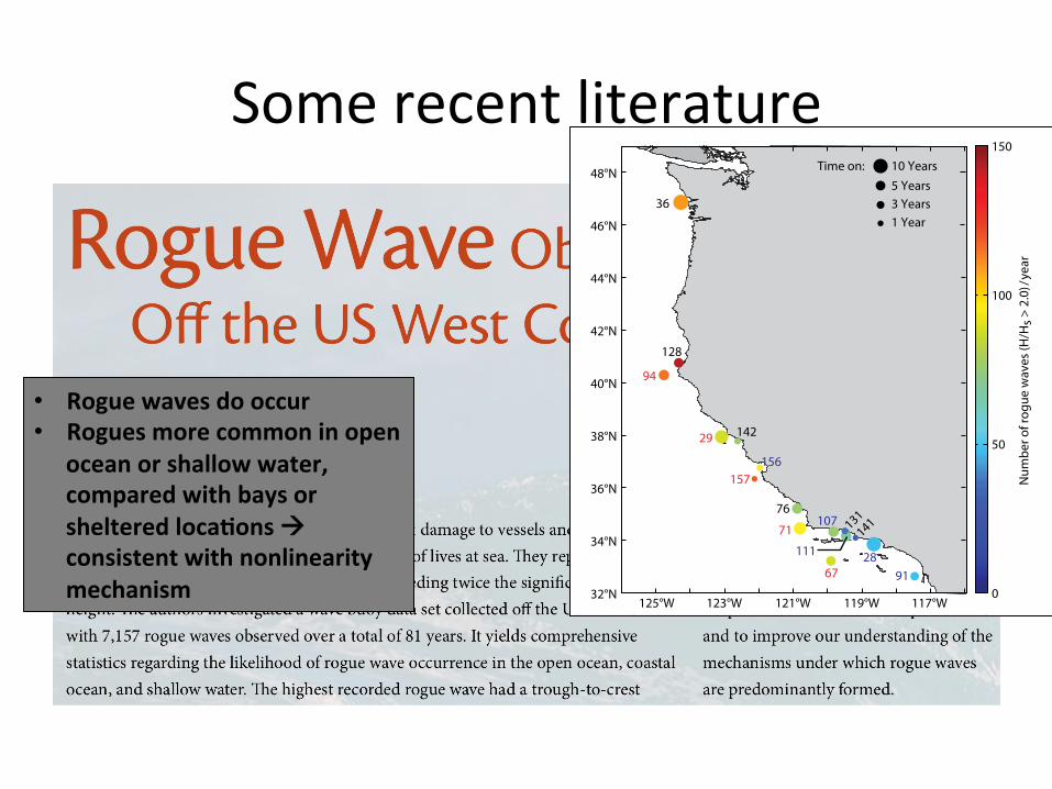
Figure 1 shows regional di&erences in the likelihood of rogue wave occurrence. #e colors show the average number of rogue waves at each of the 16 buoys, indicating that the greatest likelihood of rogue wave occurrence is at the exposed deepwater and northern buoys, while the lowest likelihood of occurrence

Burkard Baschek ([email protected]) is Assistant Professor, Department of Atmospheric and Oceanic Sciences, University of California, Los Angeles, CA, USA. Jennifer Imai is a graduate of the physics master’s program, Department of Astronomy and Physics, California State University, Long Beach, CA, USA.

125°W 123°W 121°W 119°W 117°W32°N

34°N

36°N

38°N

40°N

42°N

44°N

46°N

48°N

29

36

67

71

91

94

111

128

131141

157

10 Years5 Years3 Years1 Year

Time on:

Num

ber o

f rog

ue w

aves

(H/H

s > 2

.0)/

year

142

156

28

76107

0

50

100

150

Figure 1. Map of the US West coast with locations of the Coastal Data Information Program (CDIP) buoys used in this study (Table 1). "e text shows the mooring number, and the text color indicates open-ocean moor-ings (red), coastal moorings (blue), and shallow-water moorings (black). "e average number of rogue waves per year for a ratio of wave height to signifi-cant wave height H/Hs ≥ 2.0 is given by the colored dots, with the amount of available data indicated by their size.

•  Rogue waves do occur •  Rogues more common in open

ocean or shallow water, compared with bays or sheltered locaTons à consistent with nonlinearity mechanism


Unexpected Waves

JOHANNES GEMMRICH AND CHRIS GARRETT

Department of Physics and Astronomy, University of Victoria, Victoria, British Columbia, Canada

(Manuscript received 4 December 2007, in final form 14 March 2008)

ABSTRACT

Extreme, or “rogue,” waves are those in the tail of the probability distribution and are a matter of greatconcern and considerable research. They may be partly associated with non-Gaussian behavior caused byresonant nonlinear interactions. Here it is shown that even in a Gaussian sea, “unexpected” waves, in thesense of, for example, waves twice as large as any in the preceding 30 periods, occur with sufficientfrequency to be of interest and importance. The return period of unexpected waves is quantified as afunction of the height multiplier and prior quiescent interval for various spectral shapes, and it is shown howthe return period is modified if allowance is made for nonlinear changes in wave shape and/or a buildup ofone or more waves prior to the unexpected wave. The return period of “two-sided” unexpected waves, withsubsequent as well as prior quiescence, is also evaluated.

1. Introduction

Large ocean surface waves are a matter of great con-cern for mariners, designers of ships and offshore struc-tures such as oil platforms, and many users of the sea-shore. In many situations, the overall roughness of thesea is of primary interest, but particular attention hasbeen paid to the largest waves within a given sea state.A common criterion for designating a given wave as a“rogue” is that its trough to crest height H is at least 2.2times the significant wave height Hs, defined as fourtimes the standard deviation of the surface elevation.[See Dysthe et al. (2008) for a recent review.]

For the simple case of a narrowband spectrum oflinear and independent waves, the surface elevationdistribution is Gaussian and the height H has a prob-ability density distribution (Longuet-Higgins 1952):

P!H" #4H

Hs2 exp!$

2H2

Hs2 ". !1"

The probability that a wave exceeds %Hs is exp($2%2),or (3.4 & 10$4, 6.3 & 10$5, 3.7 & 10$6) for % # (2, 2.2,

2.5). The corresponding return periods for waves ofperiod 10 s are 8.3 h, 2 days, 1 month. For narrow-banded Gaussian seas, similar results apply for thewave crest 'c # H/2.

These results need modification if the narrowbandedassumption is relaxed (Naess 1985) or if the probabilityof rogue waves is determined from data (Forristall2005). The more rapid change in wave heights meansthat a large trough is less likely to be followed by a largecrest so that extreme wave heights are now consider-ably less common (typically by a factor of 5 or more)than in the limit of a very narrow band. Allowance mayalso be made for nonresonant nonlinearity in thewaves. In particular, allowing for phase-locked secondand higher harmonics, crests become sharper andtroughs flatter. This does not affect the distribution ofwave heights, at least for a narrowband spectrum, butdoes mean that a crest height that occurs as frequentlyas a wave height of 2.2Hs is no longer just half this but,rather, 1.34Hs for typical situations (Dysthe et al. 2008).

What has been a matter of great concern is the pos-sibility that extreme waves, whether recorded as waveheight or crest height, occur more frequently than ex-pected based on Gaussian theory, or on the modifica-tion of this theory to allow for shape changes associatedwith nonresonant nonlinear interactions. In particular,numerical simulations of a reduced equation set have

Corresponding author address: Johannes Gemmrich, Depart-ment of Physics and Astronomy, University of Victoria, Victoria,BC V8W 3P6, Canada.E-mail: [email protected]

2330 J O U R N A L O F P H Y S I C A L O C E A N O G R A P H Y VOLUME 38

DOI: 10.1175/2008JPO3960.1

© 2008 American Meteorological Society

JPO3960

•  Define anomalies relaTve to previous several waves

•  Find Hj > 2 Hi somewhat common, even without nonlinearity

Nonresonant nonlinearity

As remarked above, large waves tend to havesharper crests and flatter troughs than do sinusoids.This is a consequence of nonresonant nonlinearities; tosecond order in the wave steepness a periodic wave hasan elevation (e.g., Holthuijsen 2007)

! ! a cos" "12

ka2 cos#2"$, #4$

where % is the wave phase, kx & 2'ƒt, for a wave withwavenumber k propagating in the x direction, and a isthe amplitude of the first harmonic. The second-ordercorrection is a forced wave, nonresonant since (2ƒ, 2k)do not satisfy the dispersion relation. The correctionflattens the troughs and steepens the crests, but withoutany change in the trough to crest height for a periodicwave. Allowing for the correction has been found tobetter account for the shape of large waves (e.g.,Walker et al. 2004). Some further improvement can beobtained by allowing for even higher harmonics as well,but we restrict our analysis to allowing for the secondharmonic only so as to illustrate as simply as possiblethe consequence of nonresonant nonlinearity.

For the slowly varying wave trains considered herewe implement the correction for crest heights by deriv-ing the local frequency ƒ as the reciprocal of twice thetime from upcrossing to downcrossing, determiningk ! (2'ƒ)2/g from the dispersion relation and adding(1/2)k(2

c to the linear crest height (c. This may slightlyexaggerate the correction if the crest is not midwaybetween the up- and downcrossings, but we ignore this.We could adopt a similar procedure for trough correc-tion and would now get a slight change in the waveheight as the linear crests and troughs will be of un-equal magnitudes in a slowly varying wave train, but weignore this detail and only concern ourselves with thecorrection to the crest height.

Two minor points need to be discussed. The firstis that the mean square steepness per octave for theJONSWAP spectra is independent of ƒp, since thesteepness spectral density is proportional to ƒ&1 timesthe peak enhancement factor. Thus, even with the non-linear crest height increase, our results are independentof our arbitrary choice of ƒp ! 0.1 Hz and continue toscale in time with ƒp

&1.Second, we note that by adding the second harmonic

we are altering the spectrum of the waves. We haveignored this as the effect is small; the spectrum is in-creased by less than 1% up to 1.5ƒp, approximately 2%at 2ƒp, increasing to approximately 10% between 3ƒp

and 4ƒp by which point the spectral contribution to themean square wave height is very small.

3. Results

Figure 1 shows an example of an unexpected wave.In this case, the crest height at 374 s is 2.1 times as greatas any in the preceding 310 s, which is 31 times the peakperiod of 10 s, or 43 times the average wave period of7.1 s. In this example, there is no buildup, so the wavewould qualify as unexpected, with na ! 43 and ) ! 2.1for any value of m including zero. The crest height ofthis particular unexpected wave is 1.4Hs—greater thanthe 1.1Hs that would qualify it as a rogue wave usinglinear theory. The trough to crest height, however, isonly 1.9Hs, less than the 2.2Hs required for rogue des-ignation (though the height change from the crest to thesubsequent trough is 2.7Hs). We return later to a moregeneral discussion of the extent to which unexpectedwaves meet a criterion for designation as rogue waves.

The occurrence of the large wave in Fig. 1 followinga period of much smaller waves, purely as a conse-quence of random superposition, is not surprising quali-tatively. What is not obvious is the frequency withwhich such events occur. Figure 2 shows the return pe-riod of an unexpected wave as a function of the ampli-tude multiplier ) and number of prior waves no morethan 1/) times as big, for m ! 0, that is, allowing for nobuildup. The rows are for different sea states and thecolumns for wave height based on linear waves, crestheight (lin for linear waves and crest height (nl usingthe second-order correction described above.

For * ! 1, a wave with height H at least twice that ofany of the preceding 30 waves (corresponding to 21peak periods) occurs once every 7 + 104 peak periodson average, giving a return period of 8 days if the peakperiod of the waves is 10 s. Also for * ! 1, unexpectedcrests are more probable than unexpected waves thatare high from trough to crest; with ) ! 2 and na ! 30the return period is 4 days for the linear simulation and2 days if the nonlinear enhancement is included.

FIG. 1. An example of an unexpected wave, at 374 s, from aMonte Carlo simulation of the sea surface with linear waves ofrandom phase and spectral density corresponding to a JONSWAPspectrum with * ! 1.0 and peak period of 10 s.


Some recent literature Nonlinear Wave Statistics in a Focal Zone

T. T. JANSSEN

San Francisco State University, San Francisco, California

T. H. C. HERBERS

Naval Postgraduate School, Monterey, California

(Manuscript received 19 August 2008, in final form 20 January 2009)

ABSTRACT

In this paper, the combined effects of refraction and nonlinearity on the evolution of ocean surface wavestatistics are considered and possible implications for the likelihood of extreme waves, also known as freak orrogue waves, are examined. A frequency-angular spectrum model is derived that accounts for cubic nonlineardynamics and weak lateral homogeneity of the medium. Through Monte Carlo simulations, the evolution ofwave statistics in freely developing waves, waves over an opposing shearing current, and waves refracted overan isolated topographical feature is modeled. The simulations show that freely developing, directionallyspread wave fields generally maintain near-Gaussian statistics, which was also found in earlier modelstudies. However, the enhanced nonlinearity caused by the refractive focusing of narrowband wave fields canresult locally in strongly non-Gaussian statistics and an associated increased likelihood of extreme waveevents.

1. Introduction

Stories of unexpectedly large waves rising out of no-where and wreaking havoc in their paths have beenreported throughout maritime history (see, e.g., Draper1964, 1971; Slocum 1999; Smith 2006; Liu 2007) but thesewere invariably dismissed as part of maritime folklore,not to be taken seriously. In part, this early skepticismmay have been due to the lack of understanding of the‘‘randomness’’ of the ocean surface within the deter-ministic framework of nineteenth-century fluid dynamics,a frustration perhaps best captured by a remark as-cribed to Lord Rayleigh (Kinsman 1965) that ‘‘the basiclaw of the seaway is the apparent lack of any law.’’

It was not until after the Second World War thatstochastic process theory was successfully introduced inocean wave forecasting (Bates 1952; Kinsman 1965).Major advances in our theoretical understanding ofocean wave statistics followed (see, e.g., Hasselmann1962; Kinsman 1965; Benney and Saffman 1966; Benney

and Newell 1969) and, with the advent of moderncomputers, a rapid development of stochastic wave pre-diction models suitable for oceanic-scale wave forecast-ing became possible (e.g., WAMDI Group 1988; Tolman1991; Komen et al. 1994; Booij et al. 1999; Janssen 2004;WISE Group 2007). In this statistical framework, ex-treme waves became a reality. After all, if—from a looseuse of the central limit theorem—we assign a (near)Gaussian probability density function (pdf) to the oceansurface, such extremities must occur, only with lowprobability.

However, the inherent (weak) nonlinearity of waterwaves causes deviations from Gaussian statistics. Indeep water, second-order nonlinearity (three-wave in-teractions) causes small, local corrections to the seasurface geometry, resulting in slightly peaked crests andrelatively flat troughs (Longuet-Higgins 1963; Tayfun1980). Although such local bound modes cause (small)deviations from Gaussian statistics (in particular, non-zero skewness of the sea surface elevation), they do notdirectly affect the heights of the waves nor are theydynamically important on that order. However, weaker(higher order) interactions can approach resonance andthe associated nonlinear dynamics are more intricate.At the third order, four-wave interactions drive the

Corresponding author address: Tim T. Janssen, Department ofGeosciences, San Francisco State University, 1600 Holloway Ave.,San Francisco, CA 94132.E-mail: [email protected]


DOI: 10.1175/2009JPO4124.1

! 2009 American Meteorological Society

•  Free waves are indeed Gaussian •  RefracTve focusing (currents or

topography) gives strong enough nonlinearity to increase likelihood of rogue waves

Instead, the initially unstable wave field evolves througha strongly non-Gaussian region, after which the statis-tics return to a near-Gaussian state. The remaining de-viations from Gaussianity are due to the (locally forced)second-order bound-wave components, which affect thefree-surface geometry but are without dynamical con-sequences. In other words, unidirectional waves candevelop into a stable but strongly non-Gaussian state,but in our simulations such a state appears unavailableto directionally spread waves. From this, it would follow

that in freely developing ocean waves, gradually nar-rowing under the effects of dispersion, nonlinear insta-bility can be a determining factor in the spectral shape,but the statistics can be expected to remain close toGaussian, in accordance with what is invariably ob-served.

We hypothesized that the transformation of a wavefield in a focal zone can, if fast and strong enough tocounter the stabilizing efforts of the nonlinear cou-pling, destabilize the wave field and result in strongly

FIG. 8. Time series of normalized surface elevation h/ffiffiffiffiffiffim0p

at (a) x 5 0 and (b) x/L0 5 25.6 (along center transect, y/L0 5 6.4) and pdfs at(c) x 5 0 and (d) x/L0 5 25.6 for the same initial wave field as in Fig. 7. Shown in the figure are the Monte Carlo result (circles), Gaussianpdf (solid line), and the nonlinear pdf [Eq. (21); dashed line].

AUGUST 2009 J A N S S E N A N D H E R B E R S 1957Linear Nonlinear


Rogue waves in crossing seas: The Louis Majesty accident

L. Cavaleri,1 L. Bertotti,1 L. Torrisi,2 E. Bitner-Gregersen,3 M. Serio,4 and M. Onorato4,5

Received 27 January 2012; revised 22 March 2012; accepted 26 March 2012; published 12 May 2012.

[1] We analyze the sea state conditions during which the accident of the cruise shipLouis Majesty took place. The ship was hit by a large wave that destroyed some windowsat deck number five and caused two fatalities. Using the wave model (WAM), drivenby the Consortium for Small-Scale Modelling (COSMO-ME) winds, we perform a detailedhindcast of the local wave conditions. The results reveal the presence of two comparablewave systems characterized almost by the same frequency. We discuss such sea stateconditions in the framework of a system of two coupled Nonlinear Schrödinger (CNLS)equations, each of which describe the dynamics of a single spectral peak. For some specificparameters, we discuss the breather solutions of the CNLS equations and estimate themaximum wave amplitude. Even though, due to the lack of measurements, it is impossibleto establish the nature of the wave that caused the accident, we show that the angle betweenthe two wave systems during the accident was close to the condition for which themaximum amplitude of the breather solution is observed.

Citation: Cavaleri, L., L. Bertotti, L. Torrisi, E. Bitner-Gregersen, M. Serio, and M. Onorato (2012), Rogue waves in crossingseas: The Louis Majesty accident, J. Geophys. Res., 117, C00J10, doi:10.1029/2012JC007923.

1. Introduction

[2] Reports about very large waves, often reported asfreak or rogue waves, have become more frequent in the lastone or two decades, possibly because of the increasedattention and the ever larger number of vessels on the sea.Nikolkina and Didenkulova [2011] provide an extensive listof events. Analysis of long-term records provides contra-dictory results. Liu et al. [2010], among others, suggest thatfreak waves, however defined, are more common than peo-ple thought. On the other hand, Casas-Prat and Holthuijsen[2010] report that a wave statistics from 10 million waves indeep water is well represented for wave crests, but over-estimated for wave heights, by the conventional Rayleighdistribution. Even though the scientific community has notcome to a definite answer on the problem of formation ofrogue waves, there are a number of possible mechanismsthat are well documented for being candidates in deep water(see Kharif et al. [2009] for a recent review): (i) the linearsuperposition of waves, (ii) the interaction of waves withcurrent, and (iii) the modulational instability. In the lattercase, it can happen that statistically the probability of findingan extreme wave is well beyond the statistics derived from

linear theory or even the Tayfun [1980] second-order one[see, e.g., Onorato et al., 2006a]). However, theory andexperiments showed that, while the instability is possible ina narrow spectrum unidirectional sea [Onorato et al., 2004],the related statistics shifts back toward the Rayleigh onewhen the directional spread is increased [Onorato et al.,2009a, 2009b].[3] In 2006, Onorato et al. [2006b] proposed a new

mechanism of formation of rogue waves based on the studyof a system of coupled Nonlinear Schrödinger equations.The authors speculated that the modulational instability oftwo wave trains with similar frequencies traveling at anangle could be responsible for the formation of rogue waves.Such results have been confirmed through recent numericalsimulations of the Euler equations and experimental workperformed at the Ocean basin in the Marintek Laboratories[Toffoli et al., 2011]. Results showed that the kurtosis, ameasure of the probability of occurrence of extreme waves,depends on the angle between the crossing systems. Itsmaximum value is achieved for 40! < b < 60!, where b is theangle between the two wave systems. An explanation of thisresult can be found in Onorato et al. [2010] and will bediscussed furthermore in section 4.[4] As we will show in section 3, the accident of the Louis

Majesty ship happened in crossing sea conditions: from theanalysis of the wave spectra obtained from the hindcast ofthe storm it appears clear that, at the time of the accident,two wave systems of similar frequencies coexisted. The factthat crossing seas have the potential to create hazardousconditions for mariners is not new. Indeed,Greenslade [2001]analyzed the Sydney to Hobart yacht race that took place in1998. According to the author “it was the most disastrousevent in any offshore race held in Australian waters”. Duringthe race, a severe storm off the coast of southern New South

1Institute of Marine Sciences, CNR, Venice, Italy.2CNMCA, National Meteorological Service, Rome, Italy.3Det Norske Veritas, Høvik, Norway.4Dipartimento di Fisica Generale, Università di Torino, Torino, Italy.5Sezione di Torino, INFN, Torino, Italy.

Corresponding author: M. Onorato, Dipartimento di FisicaGenerale, Università di Torino, Via P. Giuria, 1, Torino I-10125, Italy.([email protected])

Copyright 2012 by the American Geophysical Union.0148-0227/12/2012JC007923

JOURNAL OF GEOPHYSICAL RESEARCH, VOL. 117, C00J10, doi:10.1029/2012JC007923, 2012

C00J10 1 of 8

•  two comparable wave systems characterized almost by the same frequency

•  max amplitude of CNLSE from relaTve direcTons

•  Hs was only 5, but deck dammage was a 15 m

K is the wave number of the perturbation. The solutionis periodic in space. It is straightforward to show thatfor large negative times, the solution corresponds toy0exp(if)(1 + d cos (Kx)); W is the exponential growthrate of the perturbation. In Figure 6 we show an example ofsuch solution with |y|max/|y0| = 2.4142.[16] We now turn our attention to the Louis Majesty case

and apply our NLS tool and its solutions to the sea statecondition during which the accident has happened. The goalis to verify if rogue waves (breathers) are eventually con-sistent with the sea state conditions. We have mentionedsince the beginning that the model we use should be con-sidered as a prototype whose goal is to highlight somephysical behavior rather than furnishing quantitative results.Indeed, the CNLS model requires a number of hypotheses inits derivation and just the leading order physics (whichincludes nonlinearity and dispersion) is contained. Note thatsuch approach has been very successful in the case of asingle NLS: it has been found that the breather solutions ofNLS exist also in real water (this was not obvious a priori):

they have been successfully generated in wave tank facilities[Clauss et al., 2011; Chabchoub et al., 2011; Karjanto andVan Groesen, 2010].[17] The significant wave height, Hs, at the time of the

accident was estimated around 5 m. The sea state conditionwas characterized by two wave systems with more or lessthe same amplitudes traveling at an angle. Approximately,each wave system had a significant wave height of HsA ¼HsB ¼ Hs=

ffiffiffi2p

≃ 3:5 m. Excluding the Stokes contributionwhich, for moderate steepness, brings some small asymme-tries in deep water, wave packets in each wave system arecharacterized by an amplitude y0 = 1.7 m. The frequency ofboth systems is around 0.1Hz, thereforek =w2/g =≃ 0.04m"1.The estimated steepness, estimated as HsAk/2 = y0k foreach wave system is 0.07. In the presence of a single wavesystem, the modulational instability would hardly manifestitself. However, as we have discussed, the presence of asecond wave system may cause an instability and the for-mation of a rogue wave. In order to depict the solution for thecrossing sea condition the parameter K (see equation (12))must be selected. From a physical point of view suchparameter corresponds to the wave number of the perturba-tion of the plane wave, which, given k, is related to thenumber of waves under the wave packets. Ocean wind wavepackets, depending on the spectral shape, are characterizedby an average of N = 3–5 waves under each wave packetcorresponding to 6 to 10 waves in a time series [see Onoratoet al., 2000]. For our analysis we choose N = 4 as a referencenumber; therefore,K = k/N = 0.01 m"1. We are ready to buildthe breather solution and study the dependence of its maxi-mum as a function of the angle between the two sea states. InFigure 7 we show the maximum amplitude reached by thebreather for the parameters selected before as a function ofthe angle b between the two wave systems. The figure showsthat the maximum crest (the Stokes contribution is excluded)achievable within the Akhmediev solution oscillates betweenabout 8 to 10.1 m (note that one should include the Stokescorrection to establish the crest amplitude). The amplitudeincreases for angles approaching 70.52#. For larger angles the

Figure 6. The Akhmediev solution: normalized wave enve-lope as a function of nondimensional time T and space S.

Figure 7. The maximum crest amplitude of the Akhmediev breather for the Louis Majesty sea state con-ditions as a function of the angle between the two wave systems.

CAVALERI ET AL.: THE LOUIS MAJESTY ACCIDENT C00J10C00J10

6 of 8

Some recent literature Wave Modeling—Missing the Peaks

LUIGI CAVALERI

Institute of Marine Sciences, CNR, Venice, Italy

(Manuscript received 16 June 2008, in final form 14 May 2009)

ABSTRACT

The paper analyzes the capability of the present wave models of properly reproducing the conditions duringand at the peak of severe and extreme storms. After providing evidence that this is often not the case, thereasons for it are explored. First, the physics of waves considered in wave models is analyzed. Althoughmuch improved with respect to the past, the wind accuracy is still a relevant factor at the peak of the storms.Other factors such as wind variability and air density are considered. The classical theory of wave generationby J. W. Miles’s mechanism, with subsequent modifications, is deemed not sufficiently representative of extremeconditions. The presently used formulations for nonlinear energy transfer are found to lead to too widedistributions in frequency and direction, hence reducing the input by wind. Notwithstanding some recentimprovements, the white-capping formulation still depends on parameters fitted to the bulk of the data.Hence, it is not obvious how they will perform in extreme conditions when the physics is likely to be different.

Albeit at different levels in different models, the advection still implies the spreading of energy, hencea spatial smoothing of the peaks. The lack of proper knowledge of the ocean currents is found to substantiallyaffect the identification of how much energy can—in some cases—be concentrated at a given time and lo-cation. The implementation of the available theories and know-how in the present wave models are oftenfound inconsistent from model to model. It follows that in this case, it is not possible to exchange corre-sponding pieces of software between two models without substantially affecting the quality of the results.

After analyzing various aspects of a wave model, the paper makes some general considerations. Becausewave growth is the difference between processes (input and output) involving large amounts of energy, it isvery sensitive to small modifications of one or more processes. Together with the strong, but effective, tuningpresent in a wave model, this makes the introduction of new physics more complicated. It is suggested thatfor long-term improvements, operational and experimental applications need to proceed along parallelroutes, with the latter looking more to the physics without the necessity of an immediately improved overallperformance.

In view of the forthcoming increase of computer power, a sensitivity study is suggested to identify the mostcritical areas in a wave model to determine where to invest for further improvements.

The limits on the description of the physics of the processes when using the spectral approach, particularlyin extreme conditions, are considered. For further insights and as a way to validate the present theories inthese conditions, the use is suggested of numerical experiments simulating in great detail the physical in-teraction between the lower atmosphere and the single waves.

1. What to worry about

Understanding and modeling the behavior of nature,albeit at different levels, has long been one of the maintasks of humanity. Indeed, great leaps forward have beenaccomplished during the recent centuries. In particular,sea waves, with their direct influence on seafaring andfishing, have always been at the same time a source of

wonder and observations. Humans have always tried tounderstand the rules behind a certain event, the aimbeing an improved capacity of predicting the next event.

During the last 60–70 yr, warlike and commercial in-terests have stimulated a flurry of studies related to windwaves. In connection with the unpredictable develop-ment of computer sciences, this has led to drastic im-provements in many aspects of this field. Indeed, althoughI work in this area, I am still amazed knowing that it ispossible to know with remarkable detail a few days inadvance what the wave conditions will be at a certain timeand position on the opposite side of the globe.

Corresponding author address: Luigi Cavaleri, Institute of Ma-rine Sciences, CNR, Castello 1364/A, 30122 Venice, Italy.E-mail: [email protected]

NOVEMBER 2009 C A V A L E R I 2757

DOI: 10.1175/2009JPO4067.1

! 2009 American Meteorological Society

•  Models miss the peaks •  Blame 1: wind products (and

forcing physics) •  Blame 2: currents (and refracTve

focusing)

substantially missed the buoy-measured peak waveheight. The second example (courtesy of J. Bidlot,ECMWF, 2008, personal communication) concernsnonextreme conditions at a buoy in the North PacificOcean, off the coast of Oregon. The one-month plot(March 2008) shows very clearly the repeated tendencyof the model to miss the peaks. Notice that a miss by onemodel—or better, by one system—does not implya similar miss by other centers. We will return to thematter of the behavior of different modeling systems.

Another example comes from the long-term hindcastassociated with the 40-yr European Centre for Medium-Range Weather Forecasts (ECMWF) Re-Analysis(ERA-40; Uppala et al. 2005). Caires and Sterl (2005a,b)had to make use of statistically determined enhance-ments of the peaks to match the measured wave heightsat a sufficiently good level. Notwithstanding the rela-tively coarse resolution (T159; i.e., 126 km) of the me-teorological hindcast, the ERA-40 surface winds turnedout to be of good quality, and they could not be invokedas the only source of errors. The problem is not limitedto a specific model or center. In their intercomparisonexercise involving five different operational weathercenters, Bidlot et al. (2002) noted a general tendency tounderestimate the maximum values in a storm.

Strong evidence is also derived by comparing the windand wave results obtained from running the wave modelwith the winds produced using the same meteorologicalmodel, but at different resolutions. Cavaleri and Bertotti

(2006) have used the ECMWF meteorological and WaveModel (WAM) for this purpose, with the latter run atboth global and Mediterranean scales. Their results areshown in Figs. 3 and 4 for wind and waves, respectively.The resolution considered for the meteorological, spec-tral model are T106, T213, T319, T511, T639, and T799,and corresponding to 190-, 95-, 62-, 39-, 31-, and 25-kmspatial resolutions, respectively. The WAM model wasrun with a 0.58 resolution on the globe, and a 0.258 reso-lution in the Mediterranean Sea. Several stormy periodswere considered; the diagnosis summarizes the overallresults. The diagrams show the improvements with re-spect to the T106 reference case. The results are reportedfor the oceans (NH 5 Northern Hemisphere; T 5 tropics;SH 5 Southern Hemisphere) and for the MediterraneanSea (MEDIT)—this one is considered to be representa-tive for the inner basins. Focusing on the oceans, we seefrom the left panels of Figs. 3 and 4 that at the presentresolution, T799, the results are almost asymptotic, anindication, consistent with the present statistics, that weare approaching the ideal result. However, our feeling iscompletely different once we look at the trend of themaxima in the right panels. We clearly see that there is noindication of an asympthotic trend, the diagrams literallyshooting up with increased resolution. This is a strongindication that the model maxima, for both wind andwaves, are still far, on the average, from the truth. It issignificant that there was no cyclone active on both thehemispheres during the period chosen for the simulation.

FIG. 2. Comparison between measured and modeled wave heights. (top) Extreme waveconditions during the storm of the century. Four different wave models have been used. Dotsshow the measured data (after Cardone et al. 1996). (bottom) Monthly time series (March2008) from the operational ECMWF model.


Wind measurements •  Wind speed is not wind stress – satura0on of drag may be important at high winds

•  ScaRerometer (satellite) winds not well calibrated for extreme condi0ons

Donelan et al 2004

Sugges0ons •  Models need

beRer source terms

•  Data needs more coverage (space and 0me)

Waves and the equilibrium range at Ocean Weather Station P

J. Thomson,1 E. A. D’Asaro,1 M. F. Cronin,2 W. E. Rogers,3 R. R. Harcourt,1 and A. Shcherbina1

Received 6 February 2013; revised 20 September 2013; accepted 29 September 2013.

[1] Wave and wind measurements at Ocean Weather Station P (OWS-P, 50!N 145!W) areused to evaluate the equilibrium range of surface wave energy spectra. Observations areconsistent with a local balance between wind input and breaking dissipation, as describedby Phillips [1985]. The measurements include direct covariance wind stress estimates andwave breaking dissipation rate estimates during a 3 week research cruise to OWS-P. Theanalysis is extended to a wider range of conditions using observations of wave energyspectra and wind speed during a 2 year mooring deployment at OWS-P. At moderate windspeeds (5–15 m/s), mooring wave spectra are in agreement, within 5% uncertainty, with theforcing implied by standard drag laws and mooring wind measurements. At high windspeeds (>15 m/s), mooring wave spectra are biased low, by 13%, relative to the forcingimplied by standard drag laws and mooring wind measurements. Deviations fromequilibrium are associated with directionality and variations at the swell frequencies. Aspectral wave hindcast accurately reproduces the mooring observations, and is used toexamine the wind input.

Citation: Thomson, J., E. A. D’Asaro, M. F. Cronin, W. E. Rogers, R. R. Harcourt, and A. Shcherbina (2013), Waves and theequilibrium range at Ocean Weather Station P, J. Geophys. Res. Oceans, 118, doi:10.1002/2013JC008837.

1. Introduction

[2] Ocean surface waves are the result of wind blowingalong a fetch distance for a duration of time. The evolutionof ocean surface waves is described by the wave-actionequation,

ddt

Ef

! "þ cg #r

Ef

! "¼ Swind % Sbrk þ Snl ð1Þ

in which a wave energy spectrum E(f, !) of frequency f anddirectional components ! propagates at group velocitiescg(f) and is altered by spectral source/sink terms: inputfrom the wind Swind, dissipation via breaking Sbrk, and non-linear interactions between wave frequencies Snl. This isalso called the radiative transfer equation [Young, 1999].

[3] Phillips [1985] postulated that a portion of the waveenergy spectrum would be in equilibrium such that thesource/sink terms would balance. By assuming wavegrowth to be slow and flux divergence to be negligible atsmall scales, the left-hand side of equation (1) would bezero at first order. The remaining source/sink terms on the

right-hand side then participate at first order in the equilib-rium range of the energy spectrum E. Assuming wind inputof the form Swind scales with the wind friction velocitysquared, u2

(, as empirically determined by Plant [1982],and Phillips [1985] derived an analytic expression for theenergy spectrum as a function of wave number k in theequilibrium range, which can be rewritten in terms of fre-quency f as

E fð Þ2"¼ #I pð Þgu(f %4

16"4; ð2Þ

where # is a constant, I(p) is a directional spreadingfunction, g is gravitational acceleration, and u( is thewind friction velocity. The cyclic frequency f is usedthroughout ; it is related to the radian frequency ! byf ¼ !

2". The f%4 spectral shape was first suggested as auniversal form based on observations by Toba [1973],prior to the dynamic justification proposed by Phillips[1985]. An alternate derivation based on a wave numbercascade is given by Kitaigorodski [1983]. The f%4 formis commonly used in determining the mean square slopeof a wave spectrum, which is given by

mss ¼Z

2"fð Þ4E fð Þg2

df : ð3Þ

[4] The implication of equation (2) is that, given # andI(p), wind friction velocity u( (and thus wind stress)directly controls wave energy spectra levels at high fre-quencies. More information is required, however, to com-pare wave energy spectra to a measured wind speed Uz at agiven height z (commonly U10). In a constant stress ‘‘law

1Applied Physics Laboratory, University of Washington, Seattle, Wash-ington, USA.

2Pacific Marine Environmental Laboratory, National Oceanic andAtmospheric Administration, Seattle, Washington, USA.

3Naval Research Laboratory, Stennis Space Center, Mississippi, USA.

Corresponding author: J. Thomson, Applied Physics Laboratory, Uni-versity of Washington, 1013 NE 40th St., Seattle, WA 98105, USA.([email protected])

©2013. American Geophysical Union. All Rights Reserved.2169-9275/13/10.1002/2013JC008837

1

JOURNAL OF GEOPHYSICAL RESEARCH: OCEANS, VOL. 118, 1–12, doi:10.1002/2013JC008837, 2013

dissipation at the high frequency range (0.2–0.4 Hz) of thewave energy spectrum. Using the bin-averaged results(from at least 6 h of raw data at each wind speed) of theshipboard anemometer and the SWIFTs, the wind frictionvelocities and associated wave action terms are in agree-ment over most of the range of observation conditions (3–12 m/s wind speeds).

[30] Figure 1a shows the scalar wave energy spectrafrom the SWIFTs, in which the spectral shape of f!4 is con-sistent and sorted by measured wind speeds. The equilib-rium range extends to lower frequencies during the highestwinds, consistent with the Phillips [1985] discussion ofequilibrium wave numbers and forcing scales. This is alsoconsistent with the heuristic expectation that only thewaves with phase speeds c slower than the wind speed U(i.e., ‘‘young,’’ with the wave age c

U < 1) can be forced bythe wind, and at high winds the range for which this occursis broader. For each wind speed, an equilibrium wind fric-tion velocity u" is calculated using equations (2)–(6).

[31] Figure 1b shows the wind turbulent kinetic energyspectra from the shipboard sonic anemometer, in which thef!5/3 inertial subrange is well represented and sorted bymeasured wind speeds. For each wind speed, a wind fric-tion velocity u" is estimated using equation (11) and thedissipation rate method described in section 2.1.1. Direc-tion eddy correlation estimates of u" are also used, and aresimilar to the inertial estimates. These methods avoid appli-

cation of a drag law or bulk parameterizations in validatingthe wave equilibrium results.

[32] Figure 1c shows strong agreement between the sonicfriction velocities from the two methods and the equilib-rium friction velocity. However, wave equilibrium valuesare biased low, relative to the sonic values, at higher winds.For the cruise data, the bias appears at 11 and 12 m/s,which were the highest winds observed. This is similar tothe mooring results that follow, but occurs at more moder-ate wind speeds.

[33] Figure 1 also shows dynamic evidence for waveequilibrium in source/sink terms during the October 2012mooring cruise. Application of the Phillips [1985] equilib-rium assumes a local balance, in which both wave growthand flux divergence are small. In a further simplification,integration in frequency f over the equilibrium rangeremoves the nonlinear term (because that term only redis-tributes energy in frequency), such that the balance in equa-tion (1) reduces to wind input and breaking dissipation:

0 ¼Z

Swinddf !Z

Sbrkdf : ð16Þ

[34] The wave breaking dissipation profiles fromSWIFTs during the October 2012 cruise are shown inFigure 1d and are also well sorted by measured wind speed.These values are integrated in depth (equation (8)) and

10−1

100

100

f−4(a)

f [Hz]

Wav

e E

[m2 /H

z]10

−110

0

100 f−5/3

(b)

f [Hz]

Win

d E

[m2 /s

2 /Hz]

0 1 2 3 4

x 10−3

−0.5−0.4−0.3−0.2−0.1

Dep

th z

w [m

]

Breaking dissipation εbrk [m2/s3]

U10

[m/s]

(d)

2 4 6 8 10 12

0 0.2 0.4 0.60

0.2

0.4

0.6

Sonic u* [m/s]

Equ

ilibr

um u

* [m/s

]

(c)

0 0.2 0.4 0.6 0.8 10

0.2

0.4

0.6

0.8

1

∫ Sbrk df [W/m2]

∫ Sw

ind d

f [W

/m2 ]

(e)

Equilibrium u*Inertial u*Eddy corr u*

Figure 1. Results from the shipboard and drifter measurements during the October 2012 cruise, bin-averaged and colored by observed 10 m winds on the R/V New Horizon. (a) Wave energy spectra fromSWIFT drifters. (b) Wind energy spectra from a shipboard sonic anemometer. (c) Comparison of windfriction velocity obtained via the wave equilibrium range and via the sonic anemometer using both theinertial dissipation method (open) and the direct eddy correlation method (closed). (d) Near-surface pro-files of the wave breaking dissipation rate from SWIFT drifters. (e) Terms in the theoretical equilibriumbalance of wind input and breaking dissipation. Thin lines indicate 6 one standard deviation from thebinned averages.

THOMSON ET AL.: WAVES AT STATION P

5

Conclusions & Discussion points

•  Calibra0ons and parameteriza0ons for data products and models are not well constrained for extremes –  phase resolved approaches are promising

•  Point measurements (buoys) have limita0ons –  arrays are promising

(and also phase resolving)

[email protected]

measurements of extreme waves

Documents