Measurement of the Relationship Between Oil Circulation and Compressor Lubrication

in a Mobile AlC System: Part Two

J. D. Chappell, J. C. Drozdek, C. Cusano, P. S. Hrnjak, N. R. Miller, and T. A. Newell

ACRCTR-170

For additional information:

Air Conditioning and Refrigeration Center University of Illinois Mechanical & Industrial Engineering Dept. 1206 West Green Street Urbana,IL 61801

(2,17) 333-3115

July 2000

Prepared as part of ACRC Project 92 Measurement of Oil Circulation and Compressor Lubrication in a Mobile Air Conditioning System

C. Cusano, N. R. Miller, T. A. Newell, and P. S. Hrnjak, Principal Investigators

The Air Conditioning and Refrigeration Center was founded in 1988 with a grantfrom the estate of Richard W. Kritzer, the founder of Peerless of America Inc. A State of Illinois Technology Challenge Grant helped build the laboratory facilities. The ACRC receives continuing support from the Richard W. Kritzer Endowment and the National Science Foundation. Thefollowing organizations have also become sponsors of the Center.

Amana Refrigeration, Inc. Arctelik A. S. Brazeway, Inc. Carrier Corporation Copeland Corporation DaimlerChrysler Corporation Delphi Harrison Thermal Systems Frigidaire Company General Electric Company General Motors Corporation Hill PHOENIX Honeywell, Inc. Hussmann Corporation Hydro Aluminum Adrian, Inc. Indiana Tube Corporation Invensys Climate Controls Lennox International, Inc. Modine Manufacturing Co. Parker Hannifin Corporation Peerless of America, Inc. The Trane Company Thermo King Corporation Valeo, Inc. Visteon Automotive Systems Whirlpool Corporation Wolverine Tube, Inc. York International, Inc.

For additional information:

Air Conditioning & Refrigeration Center Mechanical & Industrial Engineering Dept. University of Illinois 1206 West Green Street Urbana, IL 61801

217 3333/15

Table of Contents

Chapter Page

1. Introduction ............................................................................................................................. 1 1.1 Background ........................................................................................................................ 1 1.2 Objectives and Scope of Work ........................................................................................... 3

2. Experimental Facility .............................................................................................................. 5 2.1 Test Loop Description ........................................................................................................ 5

2.1.1 Air Loops ..................................................................................................................... 6 2.1.2 Refrigerant Loop .......................................................................................................... 6

2.2 Loop Modifications ............................................................................................................ 7 2.2.1 Oil Separation Section .................................................................................................. 7

2.3 Compressor Modifications ............................................................................................... 11 2.3.1 Contact Resistance Sensor .......................................................................................... 11 2.3.2 Dynamic Pressure Transducer .................................................................................... 12

2.4 Concentration Sensors ...................................................................................................... 12 2.5 Data Acquisition .............................................................................................................. 13

3. Chapter 3: Optical Refraction Sensors ................................................................................... 15 3.1 Introduction to Optical Refraction .................................................................................... 15

3.1.1 Film Thickness Sensor ............................................................................................... 17 3.2 Sensor Design .................................................................................................................. 18

3.2.1 Oil Return Sensor. ...................................................................................................... 18 3.3 Oil Sensor Calibration and Testing ................................................................................... 20 3.4 Oil Return Line Sensor Calibration Results ...................................................................... 22

3.4.1 Static Calibration ....................................................................................................... 22 3.4.2 In Situ Calibration ...................................................................................................... 24

3.5 Film Thickness Sensor Calibration and Results ................................................................ 26

4. Oil Shut off Experiments ....................................................................................................... 33 4.1 Motivation ....................................................................................................................... 33 4.2 Test Setup ........................................................................................................................ 34 4.3 Experimental Results and Discussion ............................................................................... 35

4.3.1 Contact Resistance ..................................................................................................... 35 4.3.1.1 CompressorCRl ................................................................................................ 35 4.3.1.2 Compressor CR3 ................................................................................................ 42 4.3.1.3 Compressors CR4 and CRS ................................................................................ 44

4.3.2 Compressor Run-In .................................................................................................... 47 4.3.3 Dynamic Pressure Transducer .................................................................................... 50

5. Slugging and Dry Start Tests ................................................................................................. 55 5.1 Introduction ...................................................................................................................... 55 5.2 Slugging Test ................................................................................................................... 56

5.2.1 Test Setup .................................................................................................................. 56 5.2.2 Test Results ............................................................................................................... 57 5.2.2.1 Contact Resistance .............................................................................................. 57 5.2.2.2 Dynamic Pressure ............................................................................................... 60

iii

5.3 Dry Start Test ................................................................................................................... 63 5.3.1 Test Setup .................................................................................................................. 63 5.3.2 Test Results ............................................................................................................... 63 5.3.2.1 Contact Resistance .............................................................................................. 63 5.3.2.2 Dynamic Pressure Transducer ............................................................................. 67

6. Conclusion and Recommendations ........................................................................................ 70 6.1 Conclusions ...................................................................................................................... 70 6.2 Future Work ..................................................................................................................... 70

Bibliography ............................................................................................................................. 72

iv

Abstract

This study used previously developed instrumentation to determine the state of

compressor lubrication in an automotive NC system during three transient tests. The

primary technique used in the study was measurement of the electrical contact resistance

at the shoe and swashplate interface. The secondary technique was dynamic

measurement of the swashplate cavity pressure.

Modifications were made to the existing test stand to allow the transient testing. The

first test was an oil run down test. This test was conducted until compressor failure

occurred. The second test was a liquid refrigerant slugging test, and the third test was a

dry start test. These tests demonstrated that the instrumentation techniques were able to

detect poor compressor lubrication conditions.

This work outlines the modifications made to the test loop and presents the results of

these transient tests. A conjecture is put forth to explain test results and possible future

work is discuss.

Chapter 1: Introduction

1.1 Background

In refrigeration applications, knowledge of the amount of oil in circulation is critical to

understanding the phenomenon of system component failure. Loss of proper lubrication for an

extended period of time will cause compressor failure. In fact, failures in mobile AlC

applications are most likely to occur at the compressor. Compressors are the only part ofthe

AlC system with complex moving parts and, therefore, are the most expensive parts of the

system. In order to reduce warranty costs in the most effective manner, it is desirable to monitor

the compressor and predict imminent compressor failure well before it occurs.

A common mode offailure ofa swashplate type automotive compressor is due to loss of

lubricating oil at the shoe and swashplate interface. While the compressor is being properly

lubricated, a film of oil is maintained between the shoe and the swashplate. This oil film

prevents the shoe and swashplate surfaces from making contact with one another. Failure at this

interface is commonly caused by a phenomenon known as scuffmg. When the shoe and

swashplate come into contact, scuffmg can be the result. Scuffmg is localized damage caused by

the occurrence of solid-phase welding between sliding surfaces without local surface melting.

For the mobile AlC compressor used in this study, the swashplate is made of 390 Al coated with

tin and the shoe is made of 521 00 Steel. Once the tin coating on the swashplate is worn through,

scuffmg can occur. During scuffmg in this type of compressor, small bits ofthe softer aluminum

swashplate are transferred to the hard steel shoe. Once material transfer occurs, the friction

between shoe and swashplate surfaces dramatically increases, eventually causing compressor

binding and failure.

To date, the link between lubrication circulation and the state of compressor lubrication is not

well understood. In mobile air conditioning systems, the lubricating oil circulates with the

refrigerant. Hence, knowledge of how the lubrication moves throughout the loop is a necessary

step in the understanding of compressor lubrication.

Current mobile AlC systems use Refrigerant 134a with a Polyalkylene Glycol (PAG)

lubricant. Based on design experience, companies within the automotive industry charge AlC

loops with enough P AG oil to maintain a steady state oil mass flow rate between 3 to 5%. The

automotive system manufacturers use the ASHRAE standard method [1] for determining the oil

and refrigerant concentrations. The ASHRAE standard method requires capturing a sample of

fluid from the liquid line of the loop. The volatile refrigerant in the sample is gradually boiled off

over a 24-hour period, leaving only the oil. Mass of the sample is measured both before and

after the boiling process, thereby allowing the concentration to be calculated.

This sampling technique only gives a good representation of oil mass flow rate when the

system is operating under steady state conditions and oil mass flow is the same at all locations

within the loop. During periods of transient operation, system components such as the

evaporator and condenser can build up oil, resulting in time varying oil mass flow at different

points within the loop. Unfortunately, transient operation has been demonstrated to be the major

culprit in compressor failure based on laboratory tests in the automotive industry. With this fact

in mind, measurement of steady state oil flow rate is not a good indication of what is occurring

during possible failure conditions. It is necessary to have a real time measurement ofthe mass

flow rate of oil at the inlet ofthe compressor to determine the link between compressor

lubrication and oil circulation.

In the past, In-Situ concentration measurement of mixture components has been

accomplished in several different ways. It was demonstrated by Baustian et al. [2], and Meyer

and Iabardo [10] that solution concentrations may be determined by measuring the speed of

sound through the fluid. This ultrasonic technique measured the time-of-flight ofa sound pulse

moving through a small distance in the fluid. Another method of concentration measurement

was through density correlations. As shown by Bayani et a!. [3], a high sensitivity density meter

was capable of refrigerant/ oil concentration measurements. Both ofthe methods described

previously require relatively expensive and bulky measuring equipment.

Optical refractometry can determine the concentration of components in a solution through

changes in refractive index. Refractive index of a solution was correlated to the oil and

refrigerant mixture concentration Newell [11]. This technique was shown to measure

concentrations in a refrigeration loop in situ by Wandell et a!. [16]. This sensor developed by

Newell was restricted to fluids with low refractive indices and was unable to measure high

percentage oil in refrigerant mixtures. The sensor used in the current study was developed with

the ability to measure fluids with high refractive indices. Hence, it was able to measure the full

concentration range of oil in refrigerant.

Investigation of transient oil movement in an automotive test loop has been accomplished in

the liquid line with optical refraction sensors developed by Wandell [17]. During Wandell's

study, mass flow rate of oil has been shown to vary as much as 1-23% for transient conditions

such as quasi-steady state clutch cycling. Although the technique used in Wandell's study can

give an accurate measurement of oil return rate to the compressor during in the steady state, it is

2

necessary to modify this technique to capture oil mass return rate during transient periods. The

measurement point in Wandell's experiments was on the opposite side of the loop from the

compressor. Measurement of concentration in the liquid line is not a good indication of oil mass

return rate to the compressor during transients, because of oil holdup in the evaporator.

Once the ability to measure oil mass return rate is obtained, compressor lubrication during

transient conditions can be studied. Due to the number and complexity of moving parts in the

compressor, instrumentation is difficult. Neither a direct nor an indirect measurement of the

lubrication of the compressor during transient conditions has been accomplished at this point in

time.

External instrumentation of the compressor housing using an Acoustic Emissions sensor was

attempted by Drozdek [7]. Surface waves at the compressor housing were measured with this

sensor; however, no link with shoe/swashplate interactions could be established with this

measurement. Drozdek also attempted internal instrumentation through the use of a contact

resistance sensor and a dynamic pressure transducer. Initial indications showed that internal

instrumentation is more successful in determining the state of compressor lubrication, this study

only included steady state conditions.

1.2 Objectives and Scope of Work

The objectives of this project are to investigate compressor failure and system lubrication.

The mechanism by which compressor failure occurs is well documented, but the lubrication

conditions that cause failure are not well understood. This investigation will serve to help

determine the link between oil return and compressor lubrication conditions.

Oil return to the compressor is studied with newly developed concentration sensors in

conjunction with previous existing compressor and loop instrumentation. All three devices are

based upon the sensor developed by Newell [11]. Oil mass flow rate is determined at three

points within the loop, in the liquid line, at the exit of the evaporator, and at the entrance to the

compressor.

Once oil mass flow is understood, it is correlated with the state of compressor lubrication.

Compressor lubrication state is determined with two sensors: a contact resistance sensor and a

dynamic pressure transducer. These internal sensing techniques investigated by Drozdek are

applied to transient conditions. These sensors measure contact resistance at the shoe/swashplate

interface and dynamic pressure in the swashplate cavity. The contact resistance and dynamic

3

pressure transducers are applied to several conditions where compressor failure is likely to occur.

The conditions studied are Oil Shut Down, Slugging, and Dry Start conditions.

4

Chapter 2: Experimental Facility

2.1 Test Loop Description

The testing facility used for experimentation is described in detail by Weston [18] and

Wandell [16] and is shown in Fig. 2.1. The test loop consists of two main parts: the air transport

loops for the evaporator and condenser, and the refrigeration loop. The air transport loops are

specially constructed and instrumented ducts. The refrigeration loop consists of the evaporator,

condenser, expansion valve, compressor, and piping between components. The evaporator,

condenser, expansion valve, liquid separator, and are standard production components from a

1994 Ford Crown Victoria. The compressor tested is a current model FS-I0 compressor.

_ -'L-..... ·-E-v.-por-a: ~;~·I

-j-- ~ Condenser Plenum

1'1 ...

Vmturifto .. T ...

- .. - I ....... IOHoad ,

Figure 2.1- Original Mobile AlC Loop Schematic

5

2.1.1 Air Loops

Air loops are built around the evaporator and condenser. Air-side pressure and temperature

measurements are made with Omega type T thermocouples and differential pressure transducers

at the inlet and outlet of both evaporator and condenser. To obtain an average temperature over

the cross-section of the ducts, 9-thermocouple grids are used at evaporator and condenser inlet

and outlets. A 7 kW electric duct heater equipped with a proportional-integral-derivative (PID)

controller is installed in the evaporator loop downstream of the evaporator. This heater insures

that the evaporator is experiencing a constant air inlet temperature. Evaporator air outlet

temperature can be controlled to an accuracy of 1°F with the electric heater. In addition, flow

mixers induce mixing of the airflow. Mixing the evaporator inlet air stream insures that the air is

at a uniform temperature at a given cross section. Reheating of evaporator exit air allows driving

conditions to be accurately simulated.

Also, a relative humidity system was installed by Whitchurch [19]. This system can control

humidity from ambient to 99% through the use of Va is ala HMP35A humidity probes upstream

and downstream of the evaporator, electrical PID controller, and electronically actuated valve.

This system is not used in these experiments.

A damper valve was installed in the condenser air loop downstream ofthe condenser to

provide control over condensing temperature. This valve allows for recirculation of warm air

from the exit of the condenser to the incoming airflow at the condenser inlet. Controlling the

proportions of recirculated and fresh air does not provide full control over condenser inlet

temperature, but allows sufficient control within the normal operational range. Airflow rates

over evaporator and condenser are controlled variable frequency drives on the blower motors.

The range of evaporator and condenser airflows achievable is well within the range present

during normal driving conditions.

2.1.2 Refrigerant Loop

Compressor speed is controlled with a 7.5 HP motor and variable frequency drive. In

automotive applications, the compressor is belted directly to the engine in an approximately I-to-

1 ratio, so normal operational speed range from idling operation to maximum engine speed is

between 800 and 6000 RPM, respectively. The operational range of the variable frequency drive

and motor combination can be greater than the normal operational range.

Mass flow can be determined in the liquid line ofthe loop. As condensed liquid exits the

condenser, the flow passes through parallel sampling sections shown in Fig. 2.2. This sampling

6

section allows for refrigerant and oil concentration to be measured at the exit of the condenser.

A Micromotion™ Coriolis type mass flow meter is installed between the test sections and the

expansion valve. This mass flow meter determines the overall refrigerant and oil mass flow in

the system. This test setup uses an orifice tube type expansion valve. Orifice size is fIXed and

can not be varied without replacing the orifice tube.

2.2 Loop Modifications

2.2.1 Oil Separation Section

1/4·in. SAE Flare NUl

1/4';11. ~ 1/4·in. SAE Flare Fitting

Removable Sampling Section

Figure 2.2- Liquid Line Sampling Sections

Initial tests to determine the lowest threshold of oil mass return rate for good compressor

lubrication were conducted by Drozdek et al [7]. For these experiments, the suction line ofthe

loop was modified from its original configuration. First, the standard suction line accumulator

was removed from the loop. Next, the original automotive refrigeration test loop was augmented

with a specially designed oil separation section shown in Figure 2.3.

The oil separation section causes liquid to be separated from the flow after the exit of the

evaporator. Refrigerant and oil exiting the evaporator is passed through a helical liquid

separator. This separator uses centrifugal acceleration to remove liquid from the flow.

7

Refrigerant and oil flow exiting the evaporator enters the separator at the top and is passed from

top to bottom ofthe separator through a helix shaped passage as seen in Figure 2.4. The liquid

component of the flow is flung to the outside of the helical separator and impacts on the outer

wall. The liquid slowly drips down the walls to the bottom ofthe separator where it exits out

through the liquid return line. The vapor is allowed to pass through the helix, up the center vapor

flow tube, and back out the top ofthe separator through the vapor return line.

Vapor

From Evaporator

Liquid

To Compressor

Sampling Section

Figure 2.3- Simplified Liquid Separation Section Schematic

Another Micromotion ™ mass flow meter is installed in the liquid return line to measure

liquid mass flow. In the separated liquid, there is still some refrigerant dissolved in the oil. This

must be accounted for to determine true oil mass flow. An oil return concentration sensor is

installed at the liquid exit of the separator in series with the mass flow meter to determine this

amount of dissolved refrigerant in the liquid flow. All of the components in the liquid return line

are connected with 6.35mm copper tubing and Swagelock brand compression fittings.

8

VaporExit _---"""r Vapor and Liquid Inlet

Liquid Exit

Figure 2.4- Cut Away of Liquid Separator

A sampling section was included in the liquid return line downstream of the mass flow meter

so that an In-Situ calibration could be performed on the concentration sensor. The sampling

section was constructed with 6.35mm (114") and 22.23mm (7/8") copper tubing and expansion

and contraction sections as shown in Figure 2.5. Two ball valves were installed on both ends of

the sampling section. The ball valves insured that both the sampling section and either end of the

liquid return line could be sealed. This prevented oil from leaking while the refrigerant sample

was being removed.

9

Compression Fig 3/8" Copper Tubing

7/8" Copper Tubing

114" Copper Tubing

Schraderer Valve

Compression Fitting

Figure 2.5- Oil Return Line Sampling Section Schematic

Two sight glasses are installed in the liquid return line to allow visual inspection of the liquid

return. The fIrst is installed upstream of the concentration sensor and the second is installed

down stream of the mass flow meter. Vapor bubbles passing through the liquid return line give

erroneous voltage readings from the concentration sensor and will give bad calibration data if the

sampling section were to contain a large portion of vapor. Visual inspection through the sight

glasses allowed bad calibration data points to be identifIed and eliminated.

Due to the slow flow rate ofliquid flow down the walls of the separator and through the

liquid return line, a signifIcant amount of heat transfer occurred between the liquid and external

environment. Ideally, a more accurate simulation of an actual system would be achieved with

recombined refrigerant and oil at the same temperature as at the exit of the evaporator. If

significant heat transfer occurred, the liquid returning out ofthe liquid return line would be

several degrees Fahrenheit warmer than the temperature at the exit of the evaporator. On the

other hand, the refrigerant vapor tends to maintain the same temperature as the fluid at the exit of

the evaporator. The warm oil and the cooler refrigerant are recombined when the liquid return

line and vapor line corne together downstream of the separator. In order to avoid this problem,

the separator was wrapped in 12.7 rnrn (W') polypropylene insulation. In addition, the liquid

return line copper tubing was insulated with 12.7 rnrn (Yz") pipe insulation cut down and taped

together to fIt the 6.35 rnrn (W') tubing. The additional thermal resistance imparted by the

insulation allowed the liquid to remain at approximately the same temperature as the fluid exiting

the evaporator.

10

2.3 Compressor Modifications

2.3.1 Contact Resistance Sensor

One promising technique to determine the state of compressor lubrication is measurement of

electrical contact resistance at the shoe/ swashplate interface. Previous work by Y oon and

Cusano [20] with a pin and disk machine has demonstrated that the contact resistance between

aluminum and steel sliding contacts is on the order of 10kO while an oil film is present. When

the oil film becomes thin and the metal asperities at the shoe and swashplate surfaces come into

contact with one another, the resistance was shown to drop dramatically to values less than 10.

A contact resistance sensor applied to an automotive swashplate compressor was developed by

Drozdek et aI. [7]. This work has shown that measurement of contact resistances in steady state

conditions is possible and gives insight into oil film conditions while the compressor is well

lubricated.

In order to create a circuit through the moving parts ofthe compressor, a specially designed

set of brushes was created to make electrical contact with the piston. The contact resistance

brushes are mounted directly over the top of a specially instrumented piston as seen in Figure

2.6. This piston has been machined with axial grooves and plated with gold along the contact

surface. The grooves insure that the brush fingers maintain contact with the piston throughout the

rotation of the compressor. Gold plating reduces the contact resistance between brush and

piston. This helps to insure that this resistance remains very small in comparison with the

resistance at the shoe and swashplate interface.

Approximately 0.5 mm of material was machined from the surface ofthe bridge of the

piston. Teflon™ insulating pads were fixed in this space with epoxy. During the rotation of the

compressor, the piston bridges sometimes make contact with the side of the swashplate due to a

moment placed on the piston through the shoe. These insulating pads were necessary in order to

insure that the piston bridge and side of the swashplate would not make electrical contact. Ifthe

bridge were to contact the side of the swashplate, the electrical circuit would be shorted, and the

contact resistance measurement would give a false indication of damaging conditions.

The electrical circuit continues from the shoe and swashplate interface up through the shaft.

A slip ring was placed on the end of the shaft to close the circuit. This slip ring allowed for

relative rotation between the shaft and data acquisition system wire connections while

maintaining the necessary electrical contact.

11

2.3.2 Dynamic Pressure Transducer

The dynamic pressure sensor was mounted over the swashplate cavity as seen in Figure 2.6.

The pressure transducer will measure pressure variations close to the swashplate as a function of

time. This technique is a less direct measurement of compressor lubrication than is the contact

resistance measurement, but pressure signatures have been shown to be indications of lack of

lubrication by Drozdek et al. [8]. Pressure signatures will serve as a predictor of lubrication loss

before it can be detected by the contact resistance measurement. These pressure signatures can

be correlated with the more direct contact resistance measurement during transient periods of

poor lubrication.

Piston Ring

Piston Grooves

Insulating Pads

Brush Assembly

Critical Shoe/ Swashplate Interfaces

Dynamic Pressure Transducer

Figure 2.6- Compressor Instrumentation Schematic

Instrumentation with a pressure transducer is a much more practical method for detection of

lubrication loss for a production vehicle. If compressor lubrication state can be correlated with

pressure signatures, a simple and reliable technique suitable for long term testing or even

production might be developed.

2.4 Concentration Sensors

Three concentration sensors are installed in the loop. The liquid line concentration sensor

developed by Wandell [17] is still present upstream ofthe expansion valve. The sensor used by

12

Wandell was replaced by a newer version ofthis type of sensor. The new liquid line sensor was

less susceptible to erroneous measurements from vapor bubbles passing through the liquid line.

The two new optical refraction sensors include oil return sensor and film thickness sensor.

The oil return sensor is located at the liquid exit of the liquid separator as previously discussed.

The film thickness sensor is located in the suction line immediately upstream of the compressor.

The film thickness sensor is installed downstream ofa straight section of36cm long, 15.88mm

(5/8") copper tubing in the suction line. In the suction line, the flow is often 2-phase in nature.

Refrigerant is in vapor phase and the oil is in liquid phase. The refrigerant forms a vapor core

while the oil is pulled along the walls. Small changes in flow area or flow direction can change

the character ofthis 2-phase flow. The length of straight tubing was installed to insure that the

oil and refrigerant 2-phase flow was fully developed after making a turn as the flow exited the

evaporator.

A second sight glass is installed in the suction line immediately downstream of the film

thickness sensor. This glass allows for inspection of the flow before entering the compressor.

The film sensor electronics housing was mounted on the Uni-strut™ suction line support

approximately 7.62cm from the sensor. The wire leads to the sensor sight glass were made as

short as possible in order to avoid electric noise induction in the circuit.

2.5 Data Acquisition

Two separate data collection systems are in the experimental facility. The first is a Hewlett-

Packard data acquisition system (DAS) 1300A VXI mainframe. The system includes a HP

E13226B 5-112 digit scanning multi-meter and three HP 1395 relay multiplexers. Data from

loop instrumentation, such as pressures, temperatures, mass flows, and sensor voltages were

acquired with this system. The loop parameters changed relatively slowly with time, so a high

sampling rate was deemed unnecessary. Loop data was taken at approximately 2 seconds per

sample. The file management was performed with a PC running HP-VEE software.

The second data-logging device was a SoMat™ Model 2500. This device allows much

higher sampling rates in comparison with the HP system. The SoMat™ device can acquire data

up to speeds of 1 00 ksamplesl s. Due to the sharp transitions of the contact resistance data and

the high bandwidth required for the dynamic pressure microphone, the data-logger was used to

acquire data at 50 ksamplesl s. Also, the film thickness data was acquired with this device

because the bandwidth of the signal was unknown. The SoMat has its own 2Mb memory

13

storage. Once data were taken, they were uploaded to a PC with TCE version 2.0.1 software.

The data was then viewed and manipulated with EASE version 3 software as shown in the

software manual [14].

14

Chapter 3: Optical Refraction Sensors

3.1 Introduction to Optical Refraction

At the temperatures and pressures present in the suction line of the system, vapor refrigerant

dissolves in the oil liquid. Therefore, measurement of the concentration of dissolved refrigerant

in oil entering the compressor was necessary to understand compressor lubrication. Initially, it

was thought that the oil mass flow rate returning to the compressor would determine the

compressor lubrication. In order to determine the mass flow of oil in circulation, it was

necessary to know the concentrations ofthe oil and the refrigerant and the total mass flow rate. It

was thought that, with real time monitoring of the percent concentration of oil possible, the state

oflubrication ofthe compressor at any given time could be determined. An oil and refrigerant

concentration sensor was developed to meet these ends.

The goal of this optical refraction technique is the measurement of the critical angle between

two media when exposed to a point light source. In the ideal case, a point source of light

originates from within a medium with a relatively high index of refraction. As the light reaches

the edge of the high index of refraction material, it encounters a second material. If this second

material has a refractive index that is higher than the first medium, then all ofthe incident light is

refracted and passed through the boundary. On the other hand, if the second medium has a lower

refractive index than the first, then some ofthe light is refracted and passed through to the

second medium and the rest is reflected back, depending on light polarization. The angle at

which the light stops passing through to the second medium and begins reflecting back is called

the critical angle. Snell's Law, shown in equation 3.1, determines the critical angle. All angles

are measured from normal at the boundary of the two media. The refractive indices for P AG and

R134a are n~ 1.5 and 1.77, respectively. Using these indices of refraction, the critical angle

determined by Snell's Law is 8~ 57.9°.

(3.1)

where the n1, 81 and n2, 82 represent the indices of refraction and light ray angles for the

higher and lower index of refraction material, respectively.

Oil Return Sensor

The overall effect of the light's interaction at the barrier ofthe two media is to create two

distinct zones. The fIrst zone in the radial direction, seen in Figure 3.1, is called the shadow

regIOn. This is the region where the emitted light is below the critical angle and passed through

15

to the second medium, creating a dark ring. The second region is the light ring. In this region,

the total reflection of incident light begins for light rays greater than the critical angle. The

distance from the point source to the beginning of the light ring will change based on the index

of refraction ofthe second medium. The higher the index of refraction ofthe second medium,

the farther the light ring moves away from the point source. The theoretical distance from the

point source to the light ring for two given indices of refraction may be calculated using the

geometry of Figure 3.1 and equation 3.1. The theoretical light ring distance is determined using

equation 3.2.

Window Coatin\

Shadow Region

Light Beam

Side View

Top View

Sapphire Window

Refigera ntl Oil Mixture

Light Ring

Figure 3.1- Ideal Oil Return Sensor Geometry

16

where: nl index of refraction of the window

n2 index of refraction of refrigerant! oil mixture

Dr light ring diameter

t thickness of the window

3.1.1 Film Thickness Sensor

(3.2)

The film thickness sensor is similar in design to the oil return line sensor, however, the

intention is not to measure the index of refraction of the oil. The goal ofthe film thickness

sensor is to measure the thickness of an oil film when in the presence of a refrigerant covering

layer. Contrary to the oil return sensor, the thickness sensor window material is Pyrex glass. All

incident light on the window passes through to the oil medium. After the light enters the oil, it

will then encounter the refrigerant layer. R134a has a lower index of refraction than oil. Total

internal reflection as described previously will occur at the oil and refrigerant boundary. At the

critical angle, the incident light will be reflected back through the oil into the glass window and

onto the photodiode. The photodiode measures a voltage proportional to the intensity of

reflected light, and hence, the oil fIlm thickness.

This refractive sensor was used to measure the oil film thickness in a sight glass in the

suction line ofthe compressor. The thickness of the oil film travelling along the wall correlated

with both oil traveling as fine droplets entrained in the refrigerant vapor flow and with total oil

mass flow rate. The oil and refrigerant are assumed to have constant indices of refraction. This

implies that the oil traveling along the tube walls has reached a steady state with respect to

refrigerant in oil concentration.

Due to the complexity of2-phase flow regimes, the sensor voltage is difficult to correlate

to an exact local fIlm thickness. As refrigerant vapor travels along the suction line the vapor

shears the liquid travelling along the wall. Eventually, shearing forces on the oil tear off small

droplets entrain them in the vapor flow, forming an oil mist. Also, the faster vapor flow also

causes waves on the surface of the oil. This causes the thickness of the film to vary locally,

however the average could be used as an indication of oil mass flow returning to the compressor.

This sensor voltage will be correlated with the results from the oil return line measurement. The

oil return line sensor could not be used during transient operation. Since transient operation is

where most of the damage occurs, this sensor could be used as an indication of oncoming failure.

17

A schematic is presented in Figure 3.2. The distance the reflected light will be returned

to the window surface can be calculated from the geometry ofthe sensor and the average

thickness of the oil film.

Oil Film

Shadow Region

3.2 Sensor Design

3.2.1 Oil Return Sensor

Light Beam

Sight Glass Lr~----~~~~~------~~VVlndow

Side View

Top View

Refrigerant Vapor

Light Ring

Figure 3.2- Ideal Film Thickness Sensor Geometry

In order to measure high percent concentrations of oil in refrigerant; it was necessary to use a

window material with a high index of refraction. Use of normal Pyrex glass as in Newell's

sensor, n= 1.6, was ruled out in this case because the index of refraction of the PAG oil was

approximately n=1.5. Low concentrations of refrigerant in oil would cause the index of the

mixture to be nearly equal to the index of refraction of the glass window. If this were to happen,

the incident light would be reflected back, but at an angle close to 90°. At high angles of

reflection such as this, a small change in reflection angle causes a large change in light ring

diameter. This results in a high scattering oflight and low reflected light level. For instance, the

18

theoretical light ring diameter for a glass window with a 5mm thickness, similar to the sensor

used in this experiment, was calculated to be 53.9mm based on equation 3.2. To lower the

critical angle, a higher refractive index material was needed. Sapphire was selected as the

window material because of its high index of refraction, n::::: 1.77. Hence, the refractive index of

the sapphire window was always significantly higher than the mixture. With the sapphire

window, the light ring diameter remained relatively small and the reflected light level high. A

sapphire window of2mm thickness was selected for the sensor. The theoretical light ring

diameter with pure PAG was calculated from equation 3.2 to be approximately 12.8mm with the

sapphire window.

Approximation of a point source of light was accomplished with a red, 680 nm, high

intensity LED. The domed surface of the LED was ground flat so that it would mount flush to

the sapphire window in order to keep the light emitting crystal as close to the window as

possible. In addition, the surface between the LED and window was covered with a thin coat of

white paint to diffuse the light in all directions. This allowed the incident light to be emitted at

all angles instead of having a large concentration oflight in the direction normal to the window

surface.

A photodiode was used to determine the distance of the reflected ring from the light source.

This photodiode was mounted at a distance from the point source such that it was able to pick up

the reflected light over the entire range of mixture concentrations. A photo diode will develop a

voltage proportional to the intensity oflight incident upon on it. Hence, the net effect was that

the sensor diode developed a voltage nearly proportional to the index of refraction ofthe fluid,

and correspondingly, the concentration of the mixture. The theoretical maximum and minimum

light ring diameters based on equation 3.2 were calculated to be 12.8mm and 7.4mm for pure

P AG (0% refrigerant in oil) and pure R134a (100% refrigerant in oil), respectively.

The sensor housing consists of two main parts: a brass, high-pressure filter body and an

electronics and optics housing box. A small hole was drilled in the bottom ofthe brass filter

body. The sapphire window was to be mounted flush with the bottom surface ofthis filter body.

A dash size 8 o-ring was installed between the housing and window to create a seal and prevent

leakage of the mixture. In addition, to reduce the error from the stray light reflected back from

the inside walls of the housing to the photodiode, the inside of the housing was painted flat

black.

19

An aluminum mounting plate machined with a hole for the LED and the photodiode was

bolted over the sapphire window. The electronics and optics housing box was mounted over the

optical window, LED, and photodiode. To condition the diode output, a simple amplifying

circuit shown in Figure 3.3 was designed and built. The conditioning circuit was mounted in the

electronics and optics housing box and the housing was mounted to the filter body section.

470kQ

12VOC 0.1 fJ.f

11~1--4

470kQ

.8 .7 .6 .5

Voltage Regulator

1. 2. 3. 4.

LED

Sensor Voltage

'-------...... I\J----+-II~-___ill

Figure 3.3- Sensor Conditioning Circuit

3.3 Oil Sensor Calibration and Testing

Two types oftests have been used to examine the sensor's sensitivity and repeatability. First,

a "static" tube test was used where the sensor measured a known refrigerant and oil

concentration. The sensor was tested with two refrigerant and oil combinations, R22/

Alkylbenzene and R134a1 P AG. The second test consists of an In-Situ test performed in the

mobile AlC loop. The static test was performed in a test section. The test section consisted of

two lengths of copper tubing along with several fittings. This test section is shown in Figure 3.4.

Known amounts of oil and refrigerant were added to the test section by mass measurement. In

this manner, a calibration for the entire range of concentrations was obtained. In addition, a type

T thermocouple was mounted directly onto the outer surface ofthe filter body. Mixture

temperatures were recorded throughout the trials to determine if the sensor exhibited temperature

sensitivity. During the static test, the refrigerant and oil mixture was continuously mixed while

the sensor voltage and mixture temperature was monitored.

20

Filter Body

Sight Glass

Power In

Y4" Copper Tubing wi compression fittings

Electronics Housing

Pressure Gauge

t Schraderer Fill Valve

Sensor Voltage Out

Figure 3.4- Static Calibration Test Section

The In-Situ calibration was performed in the mobile AlC test stand. The oil separation

section is shown in Figure 3.5. In the separation section, a sampling section was placed in series

with the optical sensor was used to catch a sample of the circulating mixture. During the

calibration, a sample ofliquid oil and refrigerant mixture was trapped in the sampling section

while the mobile AlC loop was running under steady state conditions. The sampling section was

removed from the loop and the refrigerant in the sampling section was allowed to gradually

boiled off, leaving only the oil. Concentration was determined by taking mass measurements of

the sampling section before and after the boiling process.

21

Vapor

From Evaporator

Liquid

To Compressor

Sampling Section

Figure 3.5- In-Situ Test Separation Section

3.4 Oil Return Line Sensor Calibration Results

3.4.1 Static Calibration

The fIrst combination of refrigerant and oil examined with the sensor was ofR-22 and

alkybenzene. The results ofthis calibration and a best-fit line are shown in Figure 3.6. These

results show a characteristic curve for the relationship between %R22 in alkylbenzene and the

sensor output voltage. This trend was observed for both of the refrigerant and oil combinations

tested. The voltage curve is non-linear at the extremes in concentration and linear in the middle

concentration range. These trends in sensor voltage may be a result of how the refractive index

of the refrigerant and oil mixture changes. Other likely causes for this nonlinearity are from the

sensor design. Recall the geometry of the sensor measuring the intensity of a light reflection

with a photodiode. The shape ofthis photo diode is square and the light is reflected radially from

the light source, which is circular. This shape difference may cause the edges ofthe shadow to

have a gradual decline in light intensity. Further investigation of this phenomenon is necessary

to fully understand the nonlinearity ofthe curve, but despite this observation, the correlation of

concentration to the sensor voltage proves useful for measurement of oil and refrigerant

concentration. The sensor performed well for this mixture, producing an accuracy of 1 %

throughout the entire range tested. In this static test, the sensor showed little temperature

sensitivity with this combination of refrigerant and oil.

22

100

90 CD c 80 CD N C CD

70 .c ~ « 60 .5 N N 50 0:: ~ !!... c 40 0 .. l! 30 -c CD () c 20 0 0

10

0

/ /

/ /

/ /

/ ../ I

:? ~

50 70 90 110 130 150 170 190 Sensor Voltage (mV)

Figure 3.6- Static Calibration: %R-22 in Akylbenzene vs. Sensor Voltage

The static test method was also used to examine a R-134a and PAG oil mixture. The results

of this test are shown in Figure 3.7. As the calibration of the sensor progressed, a leak in the

sensor was noticed where a rubber gasket seal was used. Initially, the seal was made with a

silicone gasket. This seal between the filter body and the sapphire window was replaced with an

O-ring seal, which has subsequently provided a more reliable seal. In this test, the output ofthe

sensor was not only a function of the concentration, but also a function of the temperature. The

O-ring caused a temperature dependence in the sensor. The temperature dependence appeared to

be due to thermal expansion and contraction of the O-ring. This affects the area of the sapphire

exposed to the mixture and, correspondingly, the intensity of light incident on the photodiode.

The temperature sensitivity ofthe sensor was repeatable and proved to be a linear relation in the

temperature range studied.

The static calibration was performed with both pure P AG oil and a commercial grade P AG

oil with additives. Throughout the full range of concentrations, little difference in the sensor

output was observed. The presence of additives in the commercial grade P AG oil caused no

change in sensor output.

23

100

90

0 80

(!) « 70 Il. c: III 60 ....

C') .... a:: 50 c: 0 .. l! 40 -c: CD (.) c: 30 0 (J

~ 0 20

10

0 30 40 50 60 70 80 90 100

Sensor Voltage (mv)

Figure 3.7- Static Calibration: %R134a in PAG vs. Sensor Voltage at Constant Temperatures

3.4.2 In Situ Calibration

A liquid separator on the suction side of a compressor was used to remove oil from the flow

in the suction line as described in Chapter 2. The refractive sensor was placed in series with a

mass flow meter in the oil return line. With the combination the mass flow meter and calibrated

concentration sensor, an accurate measurement of oil mass return to the compressor for

lubrication measurements was possible.

In order to perform an In-Situ calibration, an oil sampling section was placed immediately

downstream of the oil sensor in a vertical orientation in series with a sight glass. The sampling

section had a series of valves to isolate a sample of oil and refrigerant. To minimize measuring

error and meet space constraints, the section was flared out from the 6.35mm tubing to 22.23mm

tubing and back down to 6.35mm to allow a 50g sample, approximately, to be captured within a

small tube length. The sampling section was orientated vertically and a sight glass was installed

to verify there was no refrigerant vapor being captured in the test section. The refrigeration loop

was run until the oil concentration sensor reached a steady value. The sample section was then

closed off. Next, the section was removed from the loop, weighed, and the refrigerant was bled

out slowly. A fmal mass measurement of sampling section and lost oil allowed the concentration

to be calculated. This In-Situ technique was developed in order to periodically check sensor

24

calibration over time because sensor aging and aging of oil in the system may change sensor

calibration over time.

During the initial stages ofthe In-Situ calibration, the output ofthe sensor dropped out of

range, and it was determined the epoxy holding the LED in place had failed. After reapplying

the epoxy, it was observed the range of sensor output had been reduced. The epoxy forms an

optical coupling of the LED to the sapphire window. From this experience it was determined

that the sensor proved to be very sensitive to the optical coupling of the LED and window. A

second In-Situ calibration of the sensor was performed. The results of this In-Situ calibration for

the sensor and a best-fit line are shown in Figure 3.8.

25

• " • " , • '" ~ " . "

_ 20 C> « a. . =

• .L" " •

as

"" 15 C') .... " " .

" a:: ~ ~ r::: " " ,,' 0 ~ 10 e - " " " r::: Q) t) r:::

" " " 0 0

5

" " " """ o .,""" 20 22.5 25 27.5 30

Sensor Voltage (mV)

Figure 3.8- In-Situ Sensor Calibration Results

The calibration results demonstrated sensor voltage was linearly proportional to

concentration of refrigerant in oil. Contrary to what was observed in the static calibration, the

results of the In-Situ calibration showed little change in sensor voltage with changes in

temperature. This is mainly due to the fact that oil temperature varied only slightly between

samples. Changes in evaporator exit conditions had little effect on oil temperature in the oil

return loop.

During the course of the calibration, the refrigerant concentration in the return line stayed

approximately between 15-20% refrigerant in oil. Larger concentrations of refrigerant in oil

25

could not be measured in the test setup due to the limitations of the mass flow meter. The in-situ

calibration could not be performed with the evaporator exit in a 2-phase condition. The type of

mass flow meter used in the test setup induced a large pressure drop in its interior. With a

significant amount of refrigerant moving through the flow meter, the dissolved refrigerant had a

tendency to flash, causing inaccurate concentration measurements from the sampling section.

3.5 Film Thickness Sensor Calibration and Results

Film thickness sensor data were taken during both steady state and transient compressor

operation. This was done to correlate the sensor voltage reading with a corresponding oil mass

flow rate. To accomplish this calibration, data were taken at several different steady state oil

return rates as well as during slugging tests.

The oil surface waves showed in the diode voltage output. Peaks and valleys are seen in the

raw data. During the steady state experiments when film thickness data were taken, the

refrigerant exiting the evaporated was superheated. Thus, in the suction line, the refrigerant is

vapor and the oil travels along the bottom and sides of the tubing. This was a 2-phase flow

situation.

Film thickness was measured during several different steady oil return rates, 0.5%, 0.9%, and

1.2% concentration oil by mass. The raw data contain relatively large voltage fluctuations, so an

average voltage was computed for each oil return rate. Each steady state data set was taken at 5

kilosamples/s for approximately a 6s period. Computing the average signal voltage over this

period was an indication of the average oil film thickness on the window of the sightglass. In

addition, the standard deviation ofthe signal was calculated. The standard deviation was an

indication of the magnitude of sensor voltage variations, which should correlate with the wave

structure at the oil and refrigerant interface. The results ofthis analysis appear in Figure 3.9.

26

0.75,-------------------------------.- 0.1

0.09

Q7 r~~~~~~~~.~~~~~~~~~~~~~~~~~~ 0.08 • • • • •• 0.07 _

~ ~ • c CD 0.65 -I----------------------ir-------<"=-o--+ 0.06 .2 m m s ~ g 0.05 ~ ~ ~ ~ 0.6 0.04 ~ CD 0 c

en • Ave-;~;-·1 0.03 ~ o Std. Dev.

0.55 +---------------------------+ 0.02

0.01

0.5 -j-----,---,-------r------,----r---.....,------,----f- 0

0.00% 0.20% 0.40% 0.60% 0.80% 1.00% 1.20% 1.40% 1.60%

Overall Oil Concentration by Mass

Figure 3.9- Average Voltage and Standard Deviation for Steady State Film Thickness

Measurements

As the film thickness on the sensor increased, the average voltage decreased. Due to the

relative placement of the LED and photodiode, any increase in the light ring diameter should

decrease the light intensity on the photodiode. So, the results of the calibration made sense

because as film thickness increased the light ring diameter increased, and consequently, the

sensor voltage decreased. As the film thickness increased, the calculated standard deviation also

increased. The increase in standard deviation may be an indication of the presence of small,

surface waves. As film thickness increases, the film should be able to maintain larger surface

waves. The number of small, high frequency ripples that form on top of these larger low

frequency waves also grows as the film thickness increases. These smaller waves should

generate a larger variation in the voltage signal.

In addition to the steady state measurements, data were also taken during two liquid slugging

tests. After the loop was running under steady state conditions for several hours, the loop was

shut down and a 3.8kg refrigerant recovery tank connected to the suction line was placed in an·

ice bath. The valve on the tank was opened and the refrigerant was allowed to migrate into the

27

tank: for about 30 minutes. Approximately 75% of the refrigerant charge was collected in the

recovery tank. At this point, the tank: valve was closed and the tank was turned upside down.

Simultaneously the compressor was turned on and the tank valve was opened allowing liquid

refrigerant to be pulled into the compressor. Data were taken at a rate of 50 ksamples/s in Is

windows at lOs intervals with the film thickness sensor throughout this test. A more detailed

description of this test is provided in Chapter 5.

The average and standard deviation for the two slugging tests were calculated and plotted

versus time. The results are presented in Figure 3.10. The average sensor voltage and deviation

tends to increase during the first half of the test, but then experiences a sudden drop. After the

drop, the voltage tended to decrease and the deviation to increase. Although the exact oil flow

rate was unknown, these values agreed with the values seen during steady state. At this point

during the test, oil return from the evaporator was reestablished and oil began to flow through the

sensor.

0.9 -,---------------------------------r- 0.05

0.04

0.045 0.8 +--...---..--~-~I"-----~~----------j ~--~--~~--~---.~

0.7+-------------------------'--~

J- 0.035 ~ ~ 0.6 +------------------------I-+-Average G - I·· 0" Deviation C g' .0. 0.03 ~ :g 0.5 +------.-.. -,."',......:.----''-'-""'''''! •. .------------------1 .S;

& e'" 0.025 ~

5 0.4 ~'" ~ ~ ····0.······ e ....... <> 0.02 -g CI)

~ Q3 S 0.015 ~

0.2 -+------------...;.....-~-------------1 0.01

0.1 +---------------;,.....,.c---------------:L 0.005

0-+-----,-----,-----.----,----,-----+0

o 20 40 60 80 100 120

Time After Start of Slugging Test (s)

Figure 3.10- Average Voltage and Standard Deviation of Film Thickness Sensor During CR5

Slugging Test

At 60s after the start of the test, the sensor experienced the drop in average voltage and

deviation. This corresponded to visual observations that liquid refrigerant was no longer flowing

through the sensor. Since the index of refraction of the refrigerant was relatively low, it was

28

expected that the light ring would decrease in diameter relative to steady oil flow. Therefore, the

average voltage should increase while liquid refrigerant was flowing through the sightglass. At

this time, the liquid refrigerant had completely cleaned the sightglass of oil. This should

correspond to a true zero point for the sensor. During steady state testing with a zero oil flow

condition, the sightglass was observed to retain a small puddle of oil on the sensor surface. This

was unavoidable because the sightglass window had a small lip that tended to collect oil while

the refrigerant in the suction line was superheated. It was seen that the average voltage during

the "clean" portion ofthe slugging tests was approximately 4.8mv higher than the zero oil return

data from steady state testing. Also, the calculated standard deviation was 5 times lower at this

point in the slugging test than the value recorded during steady state testing.

To further investigate the wave structure on the oil surface, a Power Spectral Density

analysis (PSD) was performed on the raw sensor data. The sensor output was shown to be band

limited to approximately 100 Hz. The sensor components were the limiting factor. The

photo diode output was unable to respond to light variations above 100 Hz due to its long

response time. Wave structures have been shown by Jayani et al. [9] to have a maximum

frequency of20 Hz. These experiments were conducted with water as the liquid phase. Water is

less viscous than oil, therefore, the frequency content in the test loop was expected to be smaller

than 20 Hz. The operation ofthe sensor was not impeded by this limitation.

Electronic noise was determined to be present at 60,120, and 240 Hz in the raw data. This

noise was most likely induction noise from the electric drive motor. Unfortunately, this was

unavoidable due to the placement ofthe sensor in the suction line. In order to get rid of the noise

in the raw signal, the data were passed through a digital low pass filter with a cutoff frequency of

50 Hz. The power spectral densities ofthe film thickness data taken during tests of 0.5%

concentration oil by mass both before and after filtering are shown in Figures 3.11 a and b.

29

0.9

0.8

0.7

~ 0.6

~ a. iii 0.5 c: Cl (i) 0.4

0.3

0.2

0.1

o

0.9

0.8

0.7

'- 0.6

~ a. iii 0.5 c: Cl

(i) 0.4

0.3

0.2

0.1

o

Ii I WL~L. .L .... o 20 40

Ie ~

60 Frequency (Hz)

80 100

Figure 3.11a- PSD Analysis before Application of Filter

111'\ ~~I J

'W ".i~uA.~ .. I. i

o 20 40 60 80 100 Frequency (Hz)

Figure 3.11 b- PSD Analysis after Application of 50 Hz Low Pass Filter

30

120

120

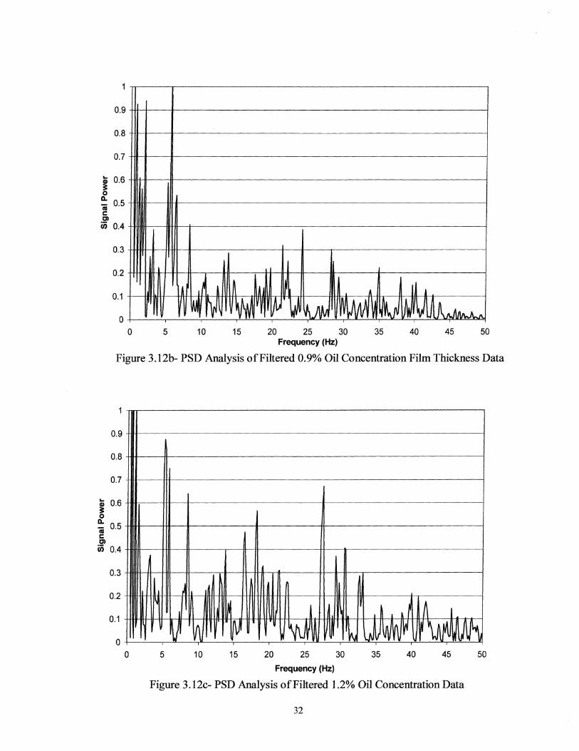
Typical samples of the PSD analyses of 0.5%, 0.9%, and 1.2% concentration oil by mass are

shown in Figures 3.12a,b, and c. The power spikes at the frequencies seen in these data moved

around in an unpredictable manner from one steady state oil concentration to another. Since only

3 oil concentration values were examined in this study, several more oil concentration values

would need to be examined to determine how these power spikes shift in frequency as a function

of oil concentration. One important observation was that the power spectrum seemed to increase

in the range from 20-50 Hz as oil concentration was increased. The increase in power for this

frequency band was most likely the reason for the increase in standard deviation with oil

concentration seen above in Figure 3.9. As power in this frequency band increased, the number

of data points above and below the mean value increased, increasing the calculated standard

deviation.

I

0.9

0.8

0.7

.. 0.6 ~ 0

Do 0.5 iii c Cl u; 0.4

0.3 /¥

0.2

0.1

~ II

0 0 5 10 15 20 25 30 35 40 45 50

Frequency (Hz)

Figure 3.12a- PSD Analysis of Filtered 0.5% Oil Concentration Film Thickness Data

31

0.9

0.8

0.7

Q; 0.6

~ a. iU 0.5 c CI ~ u; 0.4

0.3

f

II l l~jU A II M ~\ VM V~,~~ ~ lAJIM ~ ~~ ~V ~~~

0.2

0.1

o o 5 10 15 20 25 30 35 40 45 50

Frequency (Hz)

Figure 3.12b- PSD Analysis of Filtered 0.9% Oil Concentration Film Thickness Data

0.9

0.8

0.7

Q; 0.6 ~ 0 a.

0.5 iU c CI u; 0.4

0.3

0.2

0.1

0

I\J

I I , A

~ ~ irJ W ~ !~ lJiVWv /~ W\Ml ~ 0 5 10 15 20 25 30 35 40 45 50

Frequency (Hz)

Figure 3 .12c- PSD Analysis of Filtered 1.2% Oil Concentration Data

32

Chapter 4: Oil Shut off Experiments

4.1 Motivation

As described in previously by Drozdek [7], steady state operation of the system did not

significantly damage the compressor. Although regular dips in contact resistance were seen

during steady state operation, the compressor was determined to be undamaged. These contact

resistances at the shoe and swashplate interfaces were shown to be well within the resistances

associated with boundary and well-lubricated conditions. Initially, a test was performed to

determine if the compressor required a specific minimum threshold level of oil mass return to

maintain well-lubricated conditions at the shoe and swashplate interface. Drozdek determined

that this was not the case. Even a small amount of returning oil could keep the compressor well

lubricated. This was thought to be due to the long length of time oil is held up within the

compressor, maintaining the film at the swashplate surface. Although the 1000 and 10000

thresholds were demonstrated to vary with oil mass return rate, these resistance levels are not

necessarily indications of damaging conditions. These resistance levels are indications ofthinner

oil films at the interface. The 100 and tQ threshold resistance levels are indications of

damaging conditions. Drozdek demonstrated that the 100 and 10 resistance levels varied little

with varying the oil mass return rate in the range tested. To better understand compressor failure,

these steady state observations have motivated a study of possible damaging transient conditions.

In order to investigate possible failure conditions for the compressor, industry experts

were interviewed. Several common compressor failure modes are commonly seen in the field.

One common failure mode of mobile Ale compressors as describe by these experts was a low

charge failure. This type of failure occurs when a loop begins to leak some ofthe refrigerant

charge out into the atmosphere. When some ofthe refrigerant charge is leaked, refrigerant

exiting the expansion valve during operation is no longer in a 2-phase condition. The oil mass

flow rate is dramatically influenced by the refrigerant state in the liquid line. Oil mass flow rate

through the liquid line is reduced when the refrigerant is vapor. While the refrigerant is vapor,

the oil tends to form a film along the wall of the loop and is carried in the flow direction by shear

at the vapor and liquid interface. On the other hand, when the refrigerant is in the liquid state, oil

is returned easily. P AG oil is soluble in liquid R134a, so the oil is dissolved and carried along

easily by liquid refrigerant. Since a good portion ofthe oil can be retained in the evaporator,

drying out the loop downstream of the expansion valve will cause overall oil mass flow rate to

33

drop dramatically. During low refrigerant charge conditions, failure is due to lack of oil

returning to the compressor.

When the exit ofthe expansion device is 2-phase, as oil mass is retained in the

evaporator, smaller and smaller amounts of oil are returned to the compressor. The compressor

will continue pushing oil out at the rate as it would in normal steady state conditions. The

overall effect ofthis is to gradually remove oil from the interior of the compressor and put it

elsewhere in the loop. As less oil is available to form a film at the shoe and swashplate interface,

the contact resistance is expected to become smaller as the metallic surfaces begin to interact.

This is the point during low charge conditions when damage begins to occur. If it were possible

to determine when the surfaces begin to interact in a damaging manner, an appropriate feedback

device could be used to prevent further compressor damage.

This first transient test attempted to replicate this type of failure in a controlled

environment. The replication of a low charge failure is not exact in this case because ofthe

refrigerant vapor return rate to the compressor. In a field low charge failure, the overall mass of

refrigerant in the loop is reduced due to leakage, therefore the refrigerant mass flow rate is

reduced. The presence of the additional refrigerant mass in the experiment raises the heat

transfer rate inside the compressor at the critical interface. Since, scuffing failure is caused by a

combination of frictional heating and material transfer, the presence of additional refrigerant may

change the results slightly. P AG lubricant serves not only as a barrier between parts and

protecting from wear, but it also serves to cool the sliding interface. The additional refrigerant

mass flow rate in the experimental setup reduces the temperature, and hence, reduces the

frictional heating between the sliding shoe and swashplate surfaces. In the field failure, the

conditions are harsher and failure would occur in a shorter period of time due to lower heat

transfer and higher temperatures at the shoe and swashplate interface. Failure in the laboratory

setup was nearly identical, but it took a longer period oftime without oil return than would be

expected in a field failure.

4.2 Test Setup

To simulate low charge conditions, the test loop was modified as described in Chapter 1

to separate liquid from the flow exiting the evaporator. The test was run with approximately 10-

20°C of superheat at the evaporator exit in order to measure oil mass flow properly. This

insured that the liquid content of the separated fluid was mostly oil with a small portion of

34

dissolved refrigerant. Large concentrations of liquid refrigerant in the liquid line of the separator

would cause refrigerant flashing due to the pressure drop. 2-phase fluid moving through the

mass flow meter causes erroneous measurements. If the refrigerant were to flash upstream of the

mass flow meter, this would cause incorrect oil mass flow measurements. For all of the loop

conditions tested, the equilibrium concentration of refrigerant in oil in the liquid return line was

between 13-17% refrigerant by mass.

In order to perform the oil shut off test, the evaporator exit flow was forced through the

separator section. The loop was started in steady state conditions with overall oil return at

approximately 1.2% oil by mass. After the loop had been running with a steady state oil return

rate for 45-60 minutes, the liquid return valve was closed off Oil return to the compressor was

seen thorough the return line sightglass to slowly become smaller and dwindle to nothing. This

change was observed to occur within approximately a IS-minute period.

Only the refrigerant vapor was allowed to return to the compressor and the oil retained in

the compressor gradually began to exit. As the test progressed, less and less oil was available to

form the protective lubricating film causing more asperity interactions between shoe and

swashplate. This oil run down test was performed on four separate compressors, CRl, CR3,

CR4, and CRS. Two of these compressors, CRI and CR3, were run until failure and the other

two, CR4 and CR5, tested to determine if the data trends were repeatable.

4.3 Experimental Results and Discussion

4.3.1 Contact Resistance

4.3.1.1 Compressor CR1

The frrst compressor tested was CRI. This test was not conducted continuously until

compressor failure. The test was actually conducted over a three-day interval, for 3-4 hours

during each day oftesting. The test loop was started at the beginning and shut down at the end

of each day. The experimental components remained in the same state from one day to the next.

The difference between starting cold every day and running the test continuously was that the

heat generation at the shoe/swashplate surface took time to reach a steady state at the beginning

of each test day. The results from testing over a three-day interval are not expected to vary

significantly from a test conducted continuously because the system took only about 15 minutes

to come to steady state with respect to system temperatures. Due to the short amount of time

35

required to come to steady state, it is expected that the results would not significantly change

from a test that was conducted continuously.

Before compressor CRI was installed into the experimental setup, the loop was run with

a steady state oil return rate of approximately 5% oil by mass. This insured oil was distributed

throughout the loop and the compressor would receive sufficient oil return at the start of the test.

This leftover oil was then gradually removed from the loop by the liquid separator as the test

progressed. In this test, the compressor was run with steady oil return for 15 minutes before the

initiation of oil shut off. As the oil shut off was initiated, several different regimes were

observed in the contact resistance signal. Immediately following oil shut off, the raw contact

resistance was shown to drop drastically as seen in Figure 4.1. Asperity interactions appeared to

be occurring at the shoe and swashplate interfaces. The resistance dropped to around 10 for a

significant portion ofthe cycle. The test was stopped after 1 hour and the compressor opened to

perform a visual check on the swashplate. Surprisingly, some smoothing of the swashplate was

identified, but no significant damage was visible. At this point, the compressor was reinstalled

into the loop and the oil shut down test was continued.

100000~--------------------------------------------------~

14------------ One Swashplate _________________ -.1 Revolution

10000+------------------------------+--------------------~

~ E .r. 1000 Q. CD U t: .e 100 In 'iii CD a:: .... u .e 10 t: 0 0

0.1 ~----~~----------------------------------~ o 0.01 0.02 0.03 0.04 0.05 0.06 0.07 0.08

Instrumented Piston Time After TOe (s)

Figure 4.1- Raw Contact Resistance at Beginning of Oil Shut off Test

36

As the run-down ofthe fITst compressor progressed, an unexpected trend appeared. The

contact resistances throughout the cycle became higher. This rise in contact resistance occurred

between 1-2 hours after initiation of oil run down until about 30 minutes before compressor

failure. The raw contact resistance signal during this portion of the test is shown in Figure 4.2.

The raw contact resistance data during this portion of the test was similar to the contact

resistance data taken during steady state as seen in Drozdek [7]. This rise in contact resistance

may be due to either thickening of the tin oxide layer, the oil film, or smoothing of asperities on

the swashplate.

1000000,------.--------------------------------------------~

100000

Ui E 10000 .::. e. CD u C I'CS .. 1000 . !!! til CD

0:: .. U I'CS 100 C 0 0

10

1 +-----,----,-----,-----,----,,----,-----,----,,---~

o 0.01 0.02 0.03 0.04 0.05 0.06 0.07 0.08 0.09

Instrumented Piston Time After TOe (s)

Figure 4.2- Raw Contact Resistance in Middle of Oil Shut off Test

Approximately 12.5 hours after oil shut off, failure occurred. The contact resistance was

shown to drop off to levels of 0.1-0.010 during the 15 minutes directly preceding the binding of

the compressor. The raw contact resistance signal directly before failure is shown in Figure 4.3.

Not much difference can be seen visually between the raw contact resistance data during failure

and the data during run-in. The largest difference being that contact resistance during failure

reached as low as 0.010 during failure.

Failure was defined to have occurred once the motor in the test setup was unable to

maintain the torque required to turn the compressor. When the friction in the compressor

increased as the compressor carne close to failure, the motor in the test setup overheated. This

37

occurred twice in the testing of compressor CRI. In each case, the motor was shut off and

allowed to cool for 2 hours, and then the test was resumed. 12.5 hours after the initiation of oil

shut off, compressor friction became high enough to cause the magnetic clutch to slip. At this

point the compressor was opened and inspected. The swashplate surfaces appear severely

blackened and damaged on the highly loaded portion of the swashplate, but scuffing had not

occurred. The swashplate surface that was closest to the magnetic clutch was called the top of

the swashplate and the surface that was farthest from the clutch was called the bottom. The

bottom surface of the swashplate can be seen in Figure 4.4a. The portion ofthe contact

resistance data in which the lowest values were seen was the fIrst half of the revolution. This

corresponds to the downward piston compression. The bottom surface ofthe swashplate

appeared to be the more damaged than the top. From these two observations it can be concluded

that contact resistances between O.I-O.OOIQ were an indication that damage was occurring at the

swashplate surface.

1000000

100000

10000

Ui E 1000 .s:. Q. GI U 100 c lIS ... . !Il UI 10 GI

0:: ... U lIS ... C 0 0

0.1

0.01

0.001

0 0.02 0.04 0.06 0.08 0.1 0.12 0.14 0.16

Instrumented Piston Time After TOe (s)

Figure 4.3- Raw Contact Resistance Directly Before Failure of Oil Shut off Test

38

Figure 4.4a- Picture of Compressor CRI Swashplate at Conclusion of Oil Shut off Test

Compressor failure was caused by the failure of one of the piston rings. One ofthe

damaged pistons is shown in Figure 4.4b. The piston ring wore away and the metal surfaces of

both piston and corresponding bore were damaged. Although the swashplate surface did not

directly cause failure of the compressor, it is believed that friction at the swashplate surface did

indirectly cause the failure. As the shoe rides over the swash plate surface, there is a difference in

local velocities between the portion of the shoe that is closest to the center of rotation of the

swashplate and the portion of the shoe that is farthest from the center of rotation. The local

sliding velocity is highest the farther away one moves from the center of rotation. This shoe

inner and outer portion velocity difference causes a moment on the piston, driving the piston

bridge into the swashplate, and causing additional friction. At the same time, the thrust load

drives the piston head into the cylinder wall, wearing the piston ring away. In addition, the oil

during normal operation lubricates the piston and bore surfaces. The lack of oil at the piston and

bore interface during run down conditions aggravated the situation. The more friction present at

the swash plate surface, the greater the force driving the piston against the bore. This

combination ofthe lack of oil at the swashplate surface and the piston and bore surfaces was

believed to be the major cause of failure. Hence, although the tin swashplate coating does save

the swashplate surface from causing failure, the high friction at the swash plate surface is

indirectly the cause of failure.

39

Figure 4.4b- Picture of Failed Piston

In the field, the compressor is belted to a more powerful motor than is present in the test

setup. Failure in a field test would occur later because of the more powerful motor used.

However, the test motor was powerful enough to cause significant damage which would indicate

field failure was not be far behind. Overall, during the testing of CRl, contact resistance started

low, but rose as the test was continued. The contact resistance remained high throughout the

majority of the test and experienced a sudden drop offright before failure.

By examining only the raw contact resistance signal, it was difficult to determine what

was occurring at the shoe and swashplate interface. An alternative data processing technique

was developed to observe trends over time as the test progressed. Arbitrary threshold contact

resistance values were established at 1000n, lOOn, 50n, lOn, and In. Above lOOn there is

not much interaction occurring between shoe and swashplate. Boundary layer lubrication begins

to occur as the contact resistances fall to around IOn. Below In there is significant asperity

interaction occurring at the surfaces. At contact resistances below In, damage is expected to

occur. For this first oil shut offtest, the percentage of time contact resistance was below each of

these threshold levels was calculated. This calculation was performed by summing the number

of points below the given threshold level and dividing by the total number of data points.

Roughly, this calculation translates to the percentage of time during the approximately Is data

acquisition period that the contact resistance signal was below the threshold level of resistance.

The threshold analysis for the beginning and end ofthe test is shown in Figures 4.5a and b.

40

100% Oil Shut Off

Ci) > G) ..J G) U r:: J!l Ul ·iii G)

0:: "tI "0 s:. Ul 2! s:. .... 3: 0 "i III G)

E i= ::S! 0

Ci) > G)

..J G) U r:: J!l Ul ·iii G)

0:: "tI "0 s:. Ul 2! s:. .... 3: 0 "i III G)

E i= ::S! 0

90%

80%

70%

60%

50%

40%

30%

20%

10%

0% -20 o 20 40 60 80

Time After Oil Shut Off (min)

-.-<1 Ohm

-11-<10 Ohms

""""*- <50 Ohms

-e- <1 00 Ohms

--'-<1000 Ohms

100 120 140

Figure 4.5a- Threshold Analysis of Beginning of Compressor CRI Oil Shut off Test

100%

90%

80%

70%

60% -.-<1 Ohm

50% -11-<10 Ohms

""""*- <50 Ohms

40% -e-<1000hms ~------------+4---'--~-----------------'---7~

--.-<1000 Ohms

30%

20%

10%

:------.-Shut Off Motor--------: 0%

400 450 500 550 600 650

Time After Oil Shut Off (min)

Figure 4.5b- Threshold Analysis of End of Compressor CRI Oil Shut off Test

41

Even before oil shut off, the threshold resistance levels were higher than expected. This

was seen previously in the raw contact resistance signal. Immediately following oil shut off, all

threshold levels jump to higher percentages. The oil film at the shoe/swashplate interface

decreased from the lack of fresh return oil. After this initial jump, the threshold levels gradually

fall back down below the steady state values before the oil shut off. This trend in the data was

surprising because it was expected that the contact resistance would drop and stay low as more

and more swashplate damage was occurring. Correspondingly, the threshold levels would rise

and remain high. This phenomenon was investigated later in subsequent compressor testing.

After 55 minutes into the test, the threshold resistance levels stayed approximately

constant until approximately 10 hours after oil shut off. At this point compressor friction and

torque increased drastically and the resistance threshold levels experienced a corresponding rise.

After about 30 minutes at this high compressor torque condition, the test was stopped and

resumed due to motor overheating. The threshold resistance levels remained high as the test was

resumed. The test was stopped once more to allow the motor to cool. After this second test

stoppage, the compressor torque became high enough to cause the clutch to slip and the test was

concluded.

4.3.1.2 Compressor CR3

In order to clear up the differences between the expected and actual trends during the

testing of compressor CR1, another oil shut down test was performed to failure on a different

compressor. This was compressor CR3. Again, the oil shut off test was not continuous, but it

was performed over a three-day interval. Compressor CR3 was run for about 5-8 hours per day

until compressor failure occurred. Failure occurred 18.5 hours after initiation of oil shut off.

The results ofthis test are slightly different than the oil shut off of compressor CR1 as seen in the

threshold analysis of Figures 4.6a and b. Immediately following oil shut off the threshold

resistance levels climb rapidly. After the initial drop in contact resistance and corresponding rise

in threshold resistance levels, the threshold levels drop dramatically back down to about 0%

within 35 minutes after the oil shut off. The threshold resistance levels maintained around 0%

until approximately 1.75 hours before failure occurred. The threshold levels climb at that point.

42

Gi > Q) -I Q) 0 c .l!I III 'iii Q)

It: "tJ "'0 .c III e .c I-~ 0 Gi m Q)

E j::

~

100% Oil Shut Off I

90% I I

80%

70% 1i 60%

50% ~ 40%

30%

r---s.... I

~: I

20% I I

I 10% -~~

0% -35 15

-.-<1 ohm __ <10 ohms

f----

""-<50 ohms -e-<100 ohms --..<1000 ohms

l\ -65 115 165 215 265

Time After Oil Shut Off (min)

Figure 4.6a- Threshold Analysis of Beginning of Compressor CR3 Oil Shut off Test

100%r-----;=========~------------------------~Mfuo~to~rSh§ruu~tOff6ff_:~~~ -.-<1 ohms

90% +-----1 __ <10 ohms

l ""-<50 ohms ~ 80% +-----1 -e-<100ohms ~ -..<1000 ohms

S 70% t-----==========~--------------------~--~~--~++ij4~~ III

~ "tJ "'0 .c 50% +---~--------------------------------TH~----~+-~~------; e .c I- 40% +-""--~~"-------------------------+H--------r--~--~~~

~ ~ 30% +---~--------~--------------------~--~~---r-+~--~~--; Q)

E j:: 20% +---~----~~~-=--~.-----------~~~--~---.++-----r----; ~

900 950 1000 1050 100 1150

Time After Oil Shut Off (min)

Figure 4.6b- Threshold Analysis of End of Compressor CR3 Oil Shut off Test

43

The overall trends ofthe CR3 data were similar to those of CRl, however, the

magnitudes of the threshold levels were very different in the two cases. The CRI threshold

levels never approached zero as in the case ofCR3. Even during the period of time directly

before failure the threshold levels ofCRI are higher than CR3. The presence ofa rise and drop

in threshold levels immediately following the initiation of oil shut offwas consistent with the

previous test on CRI. However, the rise and drop occurred in a much shorter time interval. The

low resistance values, seen in the CRI test before the initiation of oil shut off, are not present in

the CR3 test data. These differences in threshold resistance during the data sets from

compressors CRI and CR3 may be due to compressor run-in.

The CRI oil shut offtest was performed on a brand new compressor, directly from the

factory. On the other hand, compressor CR3 was first run for approximately 6 hours under

steady state oil return conditions before the oil shut off test was initiated. The different running

time before failure in the testing ofCRl and CR3 could also be due to run-in. CRI lasted 10.5

hours after oil shut off, whereas CR3 lasted 18.5 hours before failing. In order to remove these

inconsistencies possibly associated with initial compressor run-in, all subsequent compressors

were run under steady state conditions for 6.5-9 hours before any transient testing was

performed.

4.3.1.3 Compressors CR4 and CR5

Due to the inconsistencies in the data from testing with compressors CRI and CR3, two

other oil shut off tests were performed on compressors CR4 and CR5. CR4 was tested in the

same manner as CR3. CR4 was run for approximately 6.5 hours with steady state oil return

before the oil shut off test to make sure that compressor run-in had occurred. During the oil shut

off test, the compressor was run for 120 minutes with steady oil return before the initiation of oil

return shut off. Once oil was shut off, the test was continued for 50 minutes with no oil returning

to the compressor. The test was stopped at this point to ensure failure did not occur. The data

from this test are presented in Figure 4.7. The data trends from the CR4 test are consistent with

the CR3 test data trends. After oil shut down was initiated, the 1000n, lOOn, and 50n threshold

resistance levels increased and the Ion and In decreased. However, the contact resistance

levels do not drop back down nearly as quickly as in the CR3 test. Even at the conclusion of this

test, the 1000n, lOOn, and 50n threshold levels have begun to drop down, but have not fallen

below the steady state values before oil shut off was initiated.

44

Gi > CD ..I CD (.) r:: J!l I/)

·iii CD 0:: "'C "0 r. I/)

e r. I-~ 0 Gi l'Il CD E i= ~ 0

100.0%

90.0%

80.0%

70.0%

60.0%

50.0%

40.0%

30.0%

20.0%

10.0%

0.0%

1-------1 -.-<1 ohm

___ <10 ohms

f....-----I -..- <50 ohms

-e- <1 00 ohms

..... <1000 ohms

Oil Shut Off

-120 -100 -80 -60 -40 -20 0 20 40 Time After Oil Shut Off (min)

Figure 4.7- Threshold Analysis of Compressor CR4 Oil Shut off Test

Two separate oil shut off tests were performed on the fmal compressor, CRS. The first

test was performed to verifY the trend from the testing ofCR4. The results of this test are shown

in Figure 4.8. CRS was run for approximately 9 hours with steady oil return before either ofthe

oil shut off tests was performed. This insured that complete run-in had occurred before the

initiation ofthe oil shut off so that resistance trends would not be due to compressor run-in. For

the fIrst oil shut off test, the compressor was run for about 3.S hours in steady oil return

conditions before the initiation ofthe oil shut off. Despite the fact that these two oil shut off tests

are conducted on different compressors, the steady state values before oil shut offwere

consistent with one another. The 1000n, lOOn, and son resistance levels rose immediately

following the oil return shut offand began to drop back down after 30 minutes. As in the CR4

oil shut off test, the threshold levels in the CRS test had not dropped below the steady state

values at the conclusion of the test.

45

Oil Shut Off 100% r-----------------------------------------~~~~------~

"'iii >

90%

j 80%

~ ! 70%

'iii ~ 60% "0 "0 J: 50% f J: I-

~ "'iii m Q)

E i= 20%

10%

-+-<1 ohm 1----- ___ <10 ohms

-'-<50 ohms

f--------j --&-<100 ohms

~<1000ohms

0% -250 -200 -150 -100 -50 o 50

Time After Oil Shut Off (min)

Figure 4.8- Threshold Analysis of Compressor CR5 Oil Shut off Test

For the second test performed on CR5, the oil return was shut off and turned back on.

This test was performed to help determine if the threshold resistance level trends were an

indication of shoe and swashplate surface run-in or if they were an indication of oil and

refrigerant temperature effects at the surfaces .. Iflow threshold resistance levels after oil shut

offwere an indication of compressor run-in, then the threshold levels should stay low after oil

return was reestablished because these levels would be due to the thickening of the resistive

oxide layer. However, if the resistance levels recovered to their original value before oil shut

off, then another explanation for the data trends must be found.

After the 9 hours of run-in, CR5 was run in steady state conditions for 125 minutes, oil

return was shut off, and 100 minutes later the oil return was turned back on. The results of this

test are presented in Figure 4.9. The steady state values at all the threshold levels are similar to

the two previous tests with CR4 and CR5. As the oil return is shut off, the threshold level trends

are also similar to the previous tests. The 10000, 1000, and 500 resistance levels jump up

initially and then fall back below the steady values, and the 100 and 10 resistance levels drop

and stay low while no oil is returned to the compressor. Once the oil return was turned back on,

46

the threshold levels returned to the same values as was seen in the steady state after about 20

minutes.

This test seemed to indicate that there were effects other than smoothening of the

swashplate surface contributing to the trends in contact resistance. Another plausible

explanation for the test data could be that the residual oil stuck on the surface of the swashplate

was becoming more viscous and forming a thicker film. As the mechanical friction heats the

swashplate surface with a lack of high refrigerant concentration oil returning to the compressor,

the refrigerant concentration in the oil stuck on the swashplate could be decreasing. Although no

data was available for the exact combination ofR134a and PAG used in this study, oil viscosity

tends to increase dramatically as refrigerant concentration decreases as demonstrated in the

ASHRAE Refrigeration Handbook [1]. Ifthis were the case, the shoe would have a harder time

displacing oil out from underneath it, therefore causing thicker oil films and higher contact

resistances.

100% Oil Shut Off Oil Turned On

90% 1-+<1oh~

~------~~--------------~------------~ a; >

___ <10 ohms

CD ..J 80% -6-<50 ohms CD u -e-<100 ohms c: J!l 70% III

_____ <1000 ohms

'iii CD 0:: 60% "C 0 .r:.

50% III e .r:. I-

40% ~ 0 "iii a:I 30% CD E j:: 20% ~ 0

10%

0% -140 -100 -60 -20 20 60 100 140 180

Time After Oil Shut Off (min)

Figure 4.9- Threshold Analysis ofCRS Oil Shut off and Turn Back On Test

4.3.2 Compressor Run-In

Due to the unexpected data trends during the testing of compressor CR1, further analysis

ofthe swashplate was required. A 5mm by 8mm sample was cut from the damaged portion of

47

the swashplate of CRI. It was then analyzed by Auger spectroscopy and compared with a

similar sized sample of virgin swashplate materiaL The amount of tin oxide present in the

sample from the failed compressor was determined to be approximately 4 times the amount

present in the virgin swashplate sample. One possible explanation for the rise in contact

resistance seen in the tests after oil shut off could be the thickening of the tin oxide layer on the

swashplate. Resistance of pure tin is much lower than the resistance oftin oxides. As the

compressor was damaged, there may be an additional resistance imparted by an increasing tin

oxide layer thickness. The shoe and swashplate may still be making significant contact at the

time when the contact resistance measurement is high. Based only on the contact resistance

measurement, with this extra resistance there appears to be an oil film present.

After the CRI oil shut off test, surface profile measurements were performed on the

virgin swashplates of the remaining compressors. Surface roughness measurements were made

with a DekTak3 surface profilometer. Measurements were taken at 90° intervals both on the top

and the bottom of the swashplate starting at TDC. Two traces were taken at each swashplate

position. The four measurements at each position, two on the top and two on the bottom, were

then averaged.

A second compressor, CR3, was tested in the same manner and for the same amount of

time as CRI and then disassembled for a second surface profile measurement. The second

surface profile measurement showed that initially as the compressor was run, the surfaces

became smoother. This initial smoothening ofthe swash plate is referred to as run-in. Surface

profile measurements are summarized in Figure 4.10. This was thought to be due to the tin

coating of the swashplate. The tin coating acts as a solid lubricant when the oil film is not

sufficient to maintain lubrication. As the shoe and the swashplate make contact, the tin is pushed

around the swashplate surface.

The initial swashplate surface was relatively rough. The average surface roughness was

between 40-100 nm. Then as the surfaces interact, the swashplate becomes smoother as the

microscopic peaks are knocked down and valleys are filled in. The second set of surface profile

measurements taken after 3.5 hours of steady oil return showed that the average surface

roughness decreased even during steady state operation. The surface profiles at this point in the

test were between 35-45 nm. CR3 was installed back into the loop and run for another 3.5 hours

with steady state oil return to determine if the swashplate surfaces would become any smoother.

The values of surface did not decrease during the second 3.5 hours of operation. From this test it

can be seen that the surface profiles came to a steady value within the first few hours of

48

operation. The low contact resistance measurements during the initial few minutes of the CR1

oil shut offtest may be an indication of these surface interactions and smoothening ofthe

swashplate surface.

120

100

E 80 .s as

0:: rn U)

60 G) s:::

.s::: 01 ::J 0 0:: G) 40 01 I! G)

> « 20

o

-.- ·T"" Dead 0;,;;-.. (T~ ~ - - • - - 90 after TOG (unloaded)

--.-Bottom Dead Genter

.. x.~ " .... ....

.. _--

Initial Avg

~ - -)E- - 90 before TOG (loaded)

"

~ - .... ..... -............ ....

.... ' - " ...... ":::. ..... ~------- .. .. ..::::- ........ --.. , .-- .---

----. -------:':'~.;.¥: ~~ :::-~ ~-::~~-~ ~ ~ -~ ~ = ~~ =; ---. ---

Avg after 3_5 hours of Run-In

Time When Sample was Measured

Avg after 7 hrs of Run-In

Figure 4.10- Compressor CR3 Surface Profile Summary

Due to the results from the surface profile measurements of compressors CR3, CR4 and

CR5, they were run for several hours under steady state oil return to insure that further contact

resistance results would not be obscured by the run-in process. Surface profiles ofCR4 and CR5

were taken after the steady state operation to demonstrate that these swashplates had reached a

steady value of surface roughness. It was demonstrated that the swash plates reached a steady

value of surface roughness after 6-8 hours of steady state operation. The initial surface profiles

and profiles after 8 hours of steady operation for CR4 are shown in Figure 4.11. The initial

surface roughness measurements for CR4 are less than CR3, however the average roughness

measurements follow the same trend as for CR3. The initial roughness measurements were

between 60-70 nm, after 8 hours of steady state operation, the average roughness measurements

were between 30-45 nm. This was approximately the same as CR3.

49

100

90 - .. - . Top Dead Center (TOG)

I----

80 - - • - - 90 after TOG (unloaded) -

-..-Bottom Dead Genter

E 70 - -)E- - 90 before TOG (loaded)

-

.s as 60 0:: iii 1/1

50 CI) c .c CD ::l 40 0

0::

J~.:..-:.:..---_ ,

~ ........... -~ . ~ -~ --

..... -.. -..... -~=--~~:- -'- --', ---.~ "--- ~ -. --- .'~---~. ----.

-- "" , -CI) CD 30 e!

-, -.... CI)

> « 20

10

0 Initial Avg Avg after 8 hours of run-in

Time When Sample was Measured

Figure 4.11- Compressor CR4 Surface Profile Summary

4.3.3 Dynamic Pressure Transducer

During the failure of a compressor on another ACRC project, a loud screeching occurred

that was audible to the human ear. It was thought that ifthe human ear could detect this

screeching sound during failure, perhaps a pressure transducer could detect this noise before it

became audible outside of the compressor housing. This prompted the installation of a dynamic

pressure transducer (DPX) into the swashplate cavity as described by Drozdek [7]. If this sound

were generated inside the compressor housing, a pressure transducer at this location should be

able to detect these pressure variations as the compressor becomes severely damaged. The

dynamic pressure transducer demonstrated it could detect loss of proper lubrication and

imminent failure of the compressor during the oil shut off tests.

The signal from the pressure transducer during steady oil return is shown in Figure 4.12.

The signature of the pressure signal may be due to many things, opening and closing of valves,

sound generation from moving parts, scraping ofthe shoe and swash plate surfaces, or other

sources. Unfortunately, due to the number of possible sources, the source of sound generation

could not be located during this study. However, as long as the pressure transducer showed a

signal that could be correlated to the condition of either proper lubrication or loss of lubrication,

locating the exact source of the noise was unnecessary.

50

From Figure 4.12 it can be seen that the signal had a mean level that cycles at a rate of

once per swashplate revolution. In addition to this, there are other pressure variations

superimposed on the top of this signal. In order to gain more insight into the cyclic nature of the

signal, a Fast Fourier Transform (FFT) was performed on the steady state data. A typical sample

data taken during steady state oil return after the FFT analysis is shown in Figure 4.13.

4 ~--~-----------------------------------------------r~ I

.: .. ---------One Swashplate Revolutionl-------~.: I

0

-1

-2

-3

-4

-0.01 0 0.01 0.02 0.03 0.04 0.05 0.06 0.07 0.08 0.09 Time After TOe (5)

Figure 4.12- DPX Signal During Steady Oil Return Conditions

Data taken after initiation of oil shut off showed a different pressure signature. These

differences in the signal could be detected with the naked eye as soon as 15 minutes after the

initiation of oil shut off. Contrary to what was seen in the contact resistance measurements, the

pressure signal remained approximately the same from 15 minutes after the initiation of oil shut

off to about 30 minutes before compressor failure. This signal was consistently present during

all oil shut off tests. The mean pressure signal, seen in the case of steady oil return, was still

apparent after oil return was shut off, but several regularly spaced, high frequency acoustic

events not seen during the steady state were superimposed on this bulk signal. This is seen in the

oil shut off test ofCRI shown in Figure 4.14.

51

0.1

0.Q1

Gi ~ 0 0.001 D..

iii c OJ

Ui 0.0001 >< D.. 0

0.00001

0.000001 +----l-+---'I----"-l.lJHlH-II-..... -R-I-IIt-I-II'l-aJI+hIHfJ-lIIIJ-!-....... --flI--f---1

0.0000001 -'--_______ -L-L..-_L..--.l.L--L_-'--___ ll---'-____ -'-'L..-..L-l

o 10 20 30 40 50 60 70 80 90 100 Frequency (Hz)

Figure 4.13- FFT Analysis of Steady Oil Return Data

20

.j :. One Swashplate Revolution , , 15 , ,

, ~

, , D.. 10 e iii c: C) 5 Ui ... CD U ::::I 0 "C II) c: I!! I- -5 I!! ::::I II) II)

-10 I!! Q.

-15

-20

-0.01 0 0.01 0.02 0.03 0.04 0.05 0.06 0.07 0.08 0.09

Time After TOC (s)

Figure 4.14- DPX Signal During Oil Shut off

52

The high frequency events occurred 10 times per revo lution. Some acoustic events had a

larger magnitude than others, but the number of events per revolution did stay constant.

Between data sets, the acoustic event with the highest magnitude did not stay consistently the

same event number. In some of the data sets, the highest magnitude event would be the 3rd event

and in other data sets, it would be the 6th acoustic event as in Figure 4.14. Since there are 10

compressions per cycle, 5 pistons with 2 compressions per pistons per cycle, this seemed to

imply that the acoustic events had something to do with the pistons or valves.

A FFT analysis was also performed on this data. The results are shown in Figure 4.15.

Frequency-wise there was not much of a difference between the FFT analyses of the data taken

before and after oil shut off However, the signal after oil shut offhad a power spectral density

magnitude that was an order of magnitude higher than the steady oil return signal. The

magnitude of the spikes was different for each data set, but the spike between 11-13 Hz always

had the highest magnitude within a given data set.

The large amplitude mean portion ofthe signal can be seen at approximately 12 Hz in

both Figures 4.13 and 4.15. In addition, there are several other spikes in the power spectrum at

24, 36, and around 60 Hz. For both conditions, the power spikes occur at multiples ofthe

compressor speed. These could be harmonics of the base compressor speed. Also, there appears

to be three spikes in the power spectral density around 60 Hz. This was most likely induced

electronic noise from the electric drive motor. Due to constraints of the experimental setup, the

compressor was located approximately 1m away from the motor. This and other power sources

in the lab setup could account for this spike in the power spectrum. The majority of the power in

the signal was band limited to 100 Hz. Frequencies higher than 100 Hz were either not present

in the signal or damped out.

The acoustic events observed in the raw data after oil shut off did not show up in the FFT

analysis. This was due to the nature of the acoustic signals. A FFT analysis is good for showing

signals at discrete frequencies that are continuous in the time domain. The acoustic events had a

high frequency content, but existed for only a short time period, the bursts present in the data

during periods of oil shut offwere time-limited in nature. With this fact in mind, a wavelet

analysis of this data is recommended. Wavelet analysis techniques are designed to better

describe a time-limited type of signal. A wavelet analysis should be able to detect the

differences in the pressure transducer data that were seen with the naked eye.

53

10.---------------------------------------------------.

0.1

~

CD 0.01 ;: 0 a. iii

0.001 I: C)

en >< a. 0.0001 0

0.00001

0.000001

0.0000001 0 10 20 30 40 50 60 70 80 90 100

Frequency (Hz)

Figure 4.15- FFT Analysis of Oil Shut off Data

54

Chapter 5: Slugging and Dry Start Tests

5.1 Introduction

After the oil shut off tests were performed; two other common conditions where compressor

failure might occur were examined. These conditions were slugging and dry startup. Slugging is

when the refrigerant entering the compressor is almost completely liquid. As stated previously,

oil dissolves easily in liquid refrigerant. If liquid refrigerant were to return to the compressor, it

would dissolve the lubricating oil inside the compressor and carry it out into the rest ofthe loop.

This can occur either during startup, or during steady operation.

A standard automotive system has a suction line accumulator. One ofthe purposes ofthis

accumulator is to make sure that any 2-phase liquid exiting the evaporator is trapped and not sent

directly to the compressor. The refrigerant gradually boils inside the accumulator and return to

the compressor as a vapor. During normal operation, this is enough to keep the compressor from

seeing any liquid refrigerant.

The primary situation in which liquid refrigerant entering the compressor causes problems is

during startup. Normally during startup, the suction line accumulator can prevent liquid

refrigerant from entering the compressor. In a certain case, however, the accumulator is unable

to prevent liquid from reaching the compressor. This occurs when the automobile has

experienced the greenhouse effect. When the automobile has been parked out in the sun, the

cabin tends to warm up hotter than the rest ofthe automobile. This is because the solar radiation

can enter through the windows of the vehicle, but the cabin environment does not exchange heat

with its environment effectively. The evaporator of the AlC system is located in the cabin of the

vehicle and maintains the same temperature as the cabin. On the other hand, the hood of the

vehicle reflects solar radiation and components underneath the hood remain cool relative to the

cabin. This temperature difference is enough to cause the refrigerant to evaporate from the hotter

parts of the system and condense in the colder parts ofthe system. In this situation refrigerant

tends to condense in the suction line of the compressor. When the AlC system starts, this liquid

refrigerant is drawn into the compressor and washes out the lubricating oil. As operation

continues, oil is returned from the accumulator, but there is a short period of time after startup

that the compressor receives no return oil. This is when compressor damage may possibly occur.

Dry start conditions also occur due to this same greenhouse effect phenomenon. The

difference is that thermal cycling must occur to dry out the compressor. When the vehicle is

parked outside the refrigerant migrates to the suction line and into the compressor. Then at

55

night, the temperatures inside the cabin and underneath the hood equilibrate. There is no longer

a driving force to keep the refrigerant inside the compressor and the refrigerant migrates back

into other components in the system. This migration mayor may not be a boiling process. The

process is unknown at this time.

If the migration is not a boiling process, the refrigerant stays as a liquid and gradually leaks

out of the compressor. Since the oil in the compressor dissolves in liquid refrigerant, a portion of

the oil leaves along with the refrigerant. Not all of the oil is taken at once, it requires many days

ofthermal cycling to clean the surfaces of the compressor dry. However, if the migration is not a

boiling process, the oil may not leave the compressor. Instead, the oil is cleaned off of the

critical swashplate and shoe surfaces. When the vapor refrigerant condenses during the day, it

condenses on all of the inner surfaces of the compressor. Once the refrigerant drops become

large enough, they fall to the bottom of the housing, taking the oil with them. In this manner, the

critical surfaces may be left dry and all of the oil is collected at the bottom of the compressor. If

the system is not operated during the cycling process, the compressor can be completely dried

out. Compressor damage occurs when the system is started after thermal cycling.

5.2 Slugging Test

5.2.1 Test Setup

Slugging tests were performed on two different compressors, CR4 and CRS. Special

modifications were made to the loop in order to make this test possible. A refrigerant fill port

was added to the suction line upstream of the sight glass as seen in Figure 5.1. Attached to the

fill port was a 1m piece of flexible refrigerant hosing. The other end of hosing was attached to a

6.8kg refrigerant recovery tank.

Before the slugging test was started, the loop was run for 30 minutes with a steady oil return

concentration of3% oil by mass using the oil separation section. This insured that the

compressor would receive adequate oil return after the liquid slugging. After the 30 min of

steady state oil return, the oil separation section was valved out of the loop and the loop was shut

down. The refrigerant recovery tank was placed in a 5gal bucket filled with ice water. The valve

to the tank was opened and the loop refrigerant charge was allowed to condense in the tank. The

tank was left in the ice bath for approximately 30 minutes after the loop was shut off. The slight

temperature difference between the room temperature AlC system components and the 0° C

56

walls ofthe tank caused approximately 80% of the loop refrigerant charge to condense in the

tank in this amount of time.

Liquid Line Concentration Sensor

Expansion Valve

Evaporator

Liquid Separator

Capture Tank

Condenser

Instrumented

Figure 5.1- Loop Schematic for Slugging Test

At this point, the tank valve was shut off, the tank was suspended upside down above the fill

port, and the tank was heated with a heat gun. Once the tank came back to room temperature, the

loop was started running again. Simultaneously, the tank valve was opened. Liquid refrigerant

flowed from the tank directly into the compressor. Liquid refrigerant flow as observed in the

sight glass lasted approximately 65-75s.

Due to memory constraints in the SoMat data acquisition system, measurements could not be

taken continuously during the entire test period. Instead, contact resistance and pressure

measurements were taken in approximately 1 s windows at lOs intervals. This allowed the

memory space ofthe SoMat to be broken up to cover the entire 65-75s when liquid refrigerant

was flowing through the compressor.

5.2.2 Test Results

5.2.2.1 Contact Resistance

The contact resistance changed throughout the test. As the first slugs of liquid entered the

compressor, the contact resistance raw data appeared similar to the values seen during steady

57

state testing. This was mainly due to the compressor loading. The refrigerant took about 20

seconds to redistribute itself throughout the loop. During the startup period, the pressure

differential from suction line to compressor outlet was small relative to its steady state value. As

described by Drozdek [7], the compressor loading at idling speed was dominated by the pressure

differential term. When the loading is small, there is not much of a driving force to push oil out

from underneath the shoe, allowing a thicker oil film. It makes sense that the contact resistance

was high during this part of the test.

Once the pressure differential built to its steady state level, the liquid refrigerant had started

to remove some of the oil from the swashplate surface. The contact resistance dropped for about

30 seconds. This appeared to be the time when damage may have occurred. Eventually, oil

began to return from the suction line and the oil film at the swashplate was reestablished. The

contact resistances came back up and approached steady state values.

A threshold analysis was performed on the test data. The threshold analysis of the slugging

test data from compressor CR4 is shown in Figure 5.2. The threshold levels start low, but

rapidly rise. All of the threshold levels peaked at 50 seconds after the start of slugging. The 1 n

threshold level, the level at which asperity interaction is occurring, reached as high as 65%. This

peak was short-lived, however, and the threshold levels dropped back down rapidly. The In and

Ion threshold resistance levels dropped back to their steady state values within 40 seconds from

the time when their peak values occurred. On the other hand, the 50n, lOOn, and 1000n

thresholds took approximately 34 minutes to drop back down to the values seen during steady

state. These contact resistance levels were indications ofthinner oil films, but were not

indications that damage was occurring. A steady value of oil film thickness took some time to

build back up. One possible explanation for this trend is that oil holdup in the compressor

increased. As more oil flowed into the compressor, more stuck to the swashplate and created a

thicker film. After 34 minutes had elapsed, the flow of oil entering and exiting the compressor

reached equilibrium and the threshold resistance maintained constant percentages for the rest of

the test.

58

100%

90% a; > CD 80% ...J CD U c:

70% S Ib ·iii CD 60% It: "tI '0

50% .r:. Ib 2! .r:.

40% I-~ 0 a; 30% In ~7-T----r+-----------------------~~<10hm

CD E

20% i=

___ <10 Ohms

-lII-tIi-----1'-----+---\----------------------------j -.- <50 Ohms

~ 0 -9-<100 Ohms

10% Tt--t----------+-__.;;:::--------------------I -..<1000 Ohms~----_1

0%

0 50 100 150 200 250 300 350 400 450

Time After Slugging (s)

Figure 5.2- Threshold Analysis ofCR4 Slugging Test

Compressor CR5 was tested in the same manner as CR4 to make sure the data was

repeatable. A threshold analysis was performed on the data to examine contact resistance trends

as time progressed. The results ofthe threshold analysis of the CR5 test data are similar to the

CR4 test data. Threshold resistance levels initially start low, jump up while liquid was entering

the compressor, and then return to steady state levels as oil return was reestablished. The results

of the threshold analysis ofCR5 contact resistance data are shown in Figure 5.3. The peak in the

threshold levels appeared at about the same time, 50 seconds, in this test as the previous test.

The system took about 30 minutes to reach steady state values of contact resistance. This also

was consistent with the data from the previous test.

59

l i+;{Ohm ---~ 0.8 +------fllP--t---\l------"r-~If----------------I-+-<10 Ohms f-------l

~ . -.-<50 Ohms S 0.7 ~<1000hms f-------l

·m --lIE--<1000 Ohms ~ 0.6+----~H-rH;r------~~----------------~ "C '0 ~ 0.5+----~~~~~--------~~-------------~

! ~ ~ 0.4+--~-+++~-r~~~-------~-----------~

~ ~ 0.3t-~~-+~~-----------~~~-----~~~==-----===~~~ CD E j:: 0.2 ::,e 0

0.1

0 0 50 100 150 200 250 300 350 400 450

Time After Slugging (s)

Figure 5.3- Threshold Analysis ofCR5 Slugging Test

5.2.2.2 Dynamic Pressure

Results from the dynamic pressure microphone in the slugging test are similar to the results

from the oil shut off test. At the start of the slugging test, the pressure microphone signature was

similar to the signature seen during steady state before the oil shut off test as seen in Figure 5.4a.

There appears to be a mean pressure signal oscillating once per compressor revolution. The

main difference between this signal and the signal seen during steady state was that one high

frequency acoustic burst was present each cycle. This was probably due to differences in

compressor machining.

After a few seconds, the refrigerant liquid started to enter the swashplate cavity and the

pressure began to vary wildly as shown in Figure 5.4b. During both slugging tests, the high

amplitude signal occurred approximately 10 seconds after the start of the test and continued for

30 seconds. This was due either to liquid impingement on the transducer surface, or by

refrigerant liquid boiling. The exact pressure would be highly dependent on local frictional heat

generation at the swashplate surface, liquid flow in the swashplate cavity, and transducer

location. However, this high amplitude signal may be used as an indication of the presence of

60

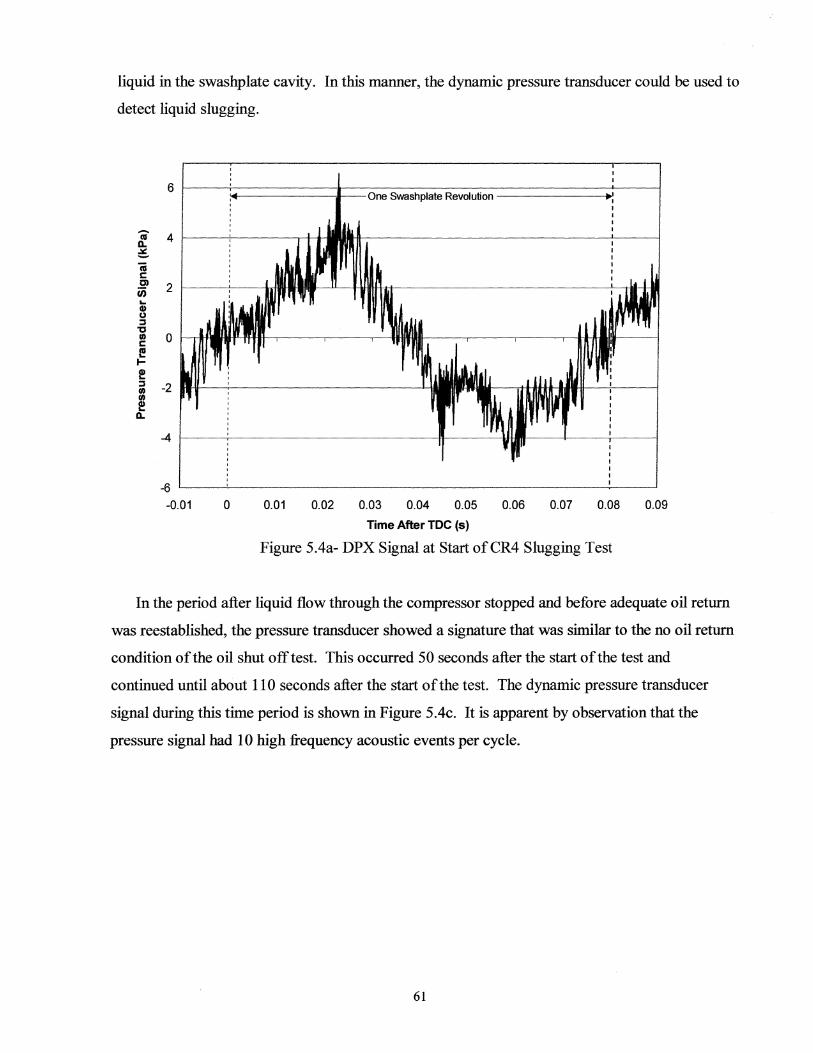
liquid in the swashplate cavity. In this manner, the dynamic pressure transducer could be used to

detect liquid slugging.

6 One Swashplate Revolution .' I I

I I

Ii ,

Go 4 ~ m t: CJ)

2 en ... CD U ::J "tJ fI) 0 t: l! l-e ::J -2 fI) fI)

e Go

-4

-6 L-__ ~ __________________________________________ ~~ __ ~

-0.01 o 0.01 0.02 0.03 0.04 0.05 0.06 0.07 0.08 0.09

Time After TOe (s)

Figure 5.4a- DPX Signal at Start ofCR4 Slugging Test

In the period after liquid flow through the compressor stopped and before adequate oil return

was reestablished, the pressure transducer showed a signature that was similar to the no oil return

condition of the oil shut off test. This occurred 50 seconds after the start of the test and

continued until about 110 seconds after the start of the test. The dynamic pressure transducer

signal during this time period is shown in Figure 5.4c. It is apparent by observation that the

pressure signal had 10 high frequency acoustic events per cycle.

61

30 r-.----~------------------------------------------------r_~

Ii 20 I a. ~ "iii 10 s:: Cl

en ... Q) U ::::I 0 "C III s:: f l-

e -10 ::::I III III e a.

-20

-30

-0.01

12

8 Ii a. ~ "iii 4 s:: Cl

en ... Q) U ::::I 0 "C III s:: f l-

e -4 ::::I III III e a.

-8

-12

I

~_--------One Swashplate Revolution -----------------.;.: :-.

0 0.01 0.02 0.03 0.04 0.05 Time After TOC (s)

0.06 0.07 0.08

I I I

Figure 5.4b- DPX Signal 20 seconds After Start ofCR4 Slugging Test

: ... --------One Swashpiate t<;e11OlUIIon ---------~.: I I I

-0.01 o 0.01 0.02 0.03 0.04 0.05 0.06 0.07 0.08

Time After TOC (s)

Figure 5.4c- DPX Signal 110 seconds After Start ofCR4 Slugging Test

62

0.09

0.09

5.3 Dry Start Test

5.3.1 Test Setup

The dry start test was also performed on two different compressors, CR4 and CRS. CR4 was

tested first. Before installing the compressor into the test setup, the inside ofthe compressor was

thoroughly cleaned. All of the inner surfaces, including the pistons, bores, valveplates,

swashplate, and shoes, were wiped with a paper towel and then wiped again with a solvent. The

solvent used was propanol. This was the most extreme possible case of dry start. During

thermal cycling, only a portion of the oil in the compressor is washed out during a given thermal

cycle. After several of these cycles, a significant portion ofthe oil is washed out, but there is still

some left when the system is started. In these tests, the compressor was completely cleaned, so

the damage was expected to be more severe than seen in a field test.

As in the slugging tests, the system was operated for about an hour with steady state 3% oil

return before the start ofthe test. This was done with a different compressor than the compressor

that was tested to insure that the compressor being tested was completely dry, yet would

experience normal oil return immediately upon startup. Once steady state was reached and held

for approximately one hour, the system was shut down and the compressors were switched. The

dry compressor was placed in the loop and the other used to bring the loop to a steady state

condition was removed.

Data was taken for approximately 5 seconds during startup. Then it was taken in I second

windows at 10 second intervals, as in the slugging test. Since the inside of the compressor was

cleaned, there was no lubricating oil on the shoe and swashplate surfaces, but there was oil in the

suction line. Oil return to the compressor would be rapid, but there would be no oil for the fIrst

few revolutions of the swashplate until the oil could be drawn into the compressor. Data was

taken in this manner because the most damage was expected to occur during the first few

revolutions of the swashplate. The rest of the available memory of the data acquisition system

was split into 1 s windows to observe changes over time.

5.3.2 Test Results

5.3.2.1 Contact Resistance

The contact resistance changed almost as was predicted. During the fIrst few seconds after

the clutch was engaged, the contact resistance was low. The contact resistance values measured

in the fIrst data set of this test were similar to the values measured during failure in the oil shut

63

off test, or at the height of the peak in the slugging test. This was somewhat surprising due to the

compressor loading. During the fIrst revolutions of the swashplate, there was not much of a

pressure differential from suction to discharge and, therefore, shoe loading should be relatively

small, yet contact resistance was low. However, the compressor seemed to recovery from this

low contact resistance condition rather rapidly. Within approximately 2 minutes after startup,

the contact resistance values measured were similar to the values seen in the steady state

measurements.

A threshold analysis of the contact resistance data from the testing ofCR4 was performed.

This is shown in Figure 5.5. The fIrst data set had low contact resistance values. The 10 and

100 threshold contact resistance levels started high. The 10 threshold level started at 22% and

the 100 threshold level started at 48%. As was evidenced by the high threshold resistances,

significant asperity interaction was occurring at the shoe and swashplate interface early in the

test. Within 3 seconds, the 10 threshold level dropped back its steady state level, and within 50

seconds, the 100 threshold level dropped back to its steady state level.

On the other hand, the 500, 1000, and 10000 levels experience a dip, jump back up, and

settle down to steady state levels 5 minutes later. Once again, these threshold resistance levels

were indications of what was happening to the oil fIlm on the swashplate. The initial burst of oil

that returns to the compressor as it is turned on was at equilibrium with the refrigerant vapor in

the suction line. As these initial droplets of oil enter the compressor they had a relatively high

viscosity and formed a thick film. As operation continues, the oil in the suction line was no

longer in equilibrium with its refrigerant surroundings and the concentration of refrigerant in the

oil becomes higher. This oil had a slightly lower viscosity than the oil that had initially coated

the swashplate, forming a thinner film and allowing the 500, 1000, and 10000 levels to

increase.

64

100%

90%

"iii > Q) 80% ..J Q) (,) I: 70% J!! 11/ ·iii Q) 60% a:

" "0 50% .I:.

11/ e .I:. I- 40% 3: 0 "iii 30% III Q)

E i= 20% :::li! 0

10%

0%

1-+-<1 ohm

-thI,----~l+tI__l_+_---------------_1---<10 ohms

-&-<50 ohms

+---'...----t\--rr------------------j-&-<100 ohms

-... <1 000 ohms

0 20 40 60 80 100 120 140 Time After Start of Test (5)

Figure 5.5- Threshold Analysis ofCR4 Dry Start Data

The same slugging test was repeated on a separate compressor, CR5, to make sure data were

repeatable. This test was performed in the same manner as the slugging test ofCR4. The results

of this test were similar to the dry start ofCR4. The raw contact resistance signal appeared low

for the fIrst few seconds of operation until oil return could be established. The contact resistance

rose to steady state levels within 15 minutes of the start of the test.

A threshold resistance analysis was performed on this data. The results are seen in Figure

5.6. Again, the 10, and 100 levels are high during the fIrst several revolutions ofthe

swashplate. The 10 threshold level started at 71 % and the 100 threshold level started at 89%.

These levels are higher than what seen during failure in the oil shut off tests, and during the peak

of the slugging tests. These low contact resistances were localized to the fIrst 4 seconds after

startup and the 10 threshold level reached its steady state value within 10 seconds after startup

as in the previous test.

The 50n, lOOn, and Iooon threshold levels started high, experienced a dip, and then

jumped back up as in the previous test. This dip in threshold levels was at fIrst thought to be

spurious data, but it was repeatable in both CR4 and CR5 tests. One possible explanation was

65

that the swashplate oil film thickness was changing due to oil viscosity changes, however,

verification of this conjecture was not possible in the course of this study. The son, lOon, and

1000n threshold levels came back up to their steady state values within 15 minutes after startup.

100% ... .... -4 ~--"--

90% CD > G)

80% ..J G) U I:

70% CIS -II) ·iii ~ 60%

" '0 50% .s::.

II)

2! .s::. ~ 40% ~ 0 a; 30% m G)

E 20% i=

~ 0

10%

-+-<1 Ohm r ~ A

__ <10 Ohms

~ \1 """'-<50 Ohms

-6-<100 Ohms lr. -lIE-<1000 Ohms

'\ \ "-~----

A y

\ \ \

--"L ~

f ..."...

ill / \ ~ -

\ - V

0% ... ~ ...... -

0 20 40 60 80 100 120 140

Time After Start of Test (s)

Figure 5.6- Threshold Analysis ofCR5 Dry Start Test Data

Most of the contact resistance trends are similar between the two tests, but there was one

major difference. The In threshold resistance level only started out at 22% in the CR4 test, yet

it started as high as 71 % in the CR5 test. This was probably due to the manner in which the data

were taken. During the CR5 test, the data were acquired during startup, but in the CR4 test, data

acquisition was started 0.5 seconds after startup. Data were not acquired during the frrst few

revolutions after the compressor clutch was engaged. It was likely that the contact threshold

value would have been this high if data acquisition was started immediately during startup

because the two threshold analyses would nearly line up if the CR4 data were shifted by this

amount.

66

5.3.2.2 Dynamic Pressure Transducer

The results of the dynamic pressure transducer measurements were similar for both CR4 and

CR5 tests. Some changes in the pressure signal were observed during the dry start tests. At the

start of the test, the dynamic pressure signal was similar to the signal seen during steady oil

return conditions. This signal seemed to indicate that the compressor was being properly

lubricated, but instead this signal was probably due to the low piston and swashplate loading at

the start of the test. If the discharge line and suction line pressures were subtracted, the pressure

differential across the compressor could be calculated as shown in Figure 5.7. This pressure

differential, within 60 seconds after startup, acted as if it was a step response to a fIrst order

system. If pressure differential were treated as a fIrst order system, the time constant ofthis

system would be approximately 8 seconds. The signal from the first data set was taken while the

pressure differential was ramping up. The pressure transducer signal taken about I s after startup

is seen in Figure 5.8a.

140

120

100

'iii 80 E: ~ ::l III III ~ 60

D..

40

20

0

,rzi

~

_ B- -13- _ s- -13- - a' -13- - a' -13- - 8- - 13--

13-- 13-

.13-- B --B"'

I

13-. 13'-

.B··B-·' 8"S-- B -

- -<) - Suction Pressure

+--+-----------------------1 .. (]. - Discharge Pressure

-4-Pressure Differential ----.--.--.-~

0 10 20 30 40 50 60 Time After Start of Test (s)

Figure 5.7- Loop Pressures during Dry Start Test

The next set of data was taken 10 seconds later. The high frequency acoustic bursts observed

during the oil shut off test were also present in this data as shown in Figure 5.8b. The pressure

differential at the point this data were taken was 77% of the steady state value. At this point in

67

the test the piston and shoe loading was close to its value during steady state, but the oil in the

suction line did not yet fully lubricate the swashplate as demonstrated by the contact resistance

data. This may explain why the acoustic bursts were present in the transducer data.

1\1 a. :. 1\1 C Cl

c;; ... CD U ::l "C I/) c f I-

15 r---~-----------------------------------------------.--' I

.' .. ----------- One Swashplate Revolution,------------------.:~'

10 ~--+-----+f-tj-

5 ~--~--UM ~----------~.~~----------------------+-~

o

~ -5 ~--_+_--------------------------~~~~~~~~~--T_~ I/) I/)

f a.

-10 ~--~--------------------------------------------+-~

-15 L-__ ~ __________________________________ . ____________ L_~

-0.01 o 0.01 0.02 0.03 0.04 0.05 0.06 0.07 0.08 0.09 Time After TOe (5)

Figure 5.8a- DPX Signal at Beginning of Compressor CR4 Dry Start Test

In both dry start tests the acoustic bursts appeared only briefly for between 10-20 seconds.

After that, the pressure transducer returned to showing the same signature seen during well­

lubricated conditions. The pressure transducer signal stayed the same for the remainder of the

test. This was because, although the piston and shoe loading was at its steady state value, the

compressor had received enough oil return to lubricate the compressor surfaces and form a film

on the swashplate surface. The pressure transducer signal 40 seconds after the start of the test is

shown in Figure 5.8c.

68

15 , , One Swashplate Revolution .' , , , , ,

~ 10

a.. ::. iii c Cl en 5 ... (i) () ::J '0 (1) c l! 0 l-

e ::J (1) (1)

e a.. -5

-10 -0.01 o 0.01 0.02 0.03 0.04 0.05 0.06 0.07 0.08 0.09

Time After TOC (5)

Figure 5.8b- DPX Signal 15 seconds after Beginning of Compressor CR4 Dry Start Test

15 l

, l : .. One Swashplate Revolution ••

iii 10 a.. ::. iii c Cl

en 5 ... (i) () ::J '0 (1) c l! 0 l-

e ::J (1) (1)

e a.. -5

-10 -0.01 o 0.01 0.02 0.03 0.04 0.05 0.06 0.07 0.08 0.09

Time After TOC (5)

Figure 5.8c- DPX Signal 30 seconds after Beginning of Compressor CR4 Dry Start Test

69

Chapter 6: Conclusion and Recommendations

6.1 Conclusions

Experimental results and the previous analyses have shown:

• The oil concentration sensor was able to measure high concentrations of oil in refrigerant.

This sensor showed a temperature sensitivity during the static calibration, however this

temperature dependence disappeared during the In Situ calibration. A linear best fit line

was found for oil concentration vs. sensor voltage for the In Situ calibration.

• The film thickness sensor was determined to have the ability to measure oil film

thickness in the suction line. The average sensor voltage decreased with increasing film

thickness. In addition, the filtered sensor output was determined to show larger signal

variation with increasing film thickness. This corresponded to increasing the power in

the frequency range 20-50Hz.

• The contact resistance was shown to decrease dramatically during the fmal stages of oil

shut off tests during the 30 minutes before compressor failure. Also, the contact

resistance thresholds, which are possible indications of compressor damage, started low,

peaked, and returned to steady state levels during slugging tests. Finally, during dry start

tests, high threshold resistance levels were limited to the frrst 1-2 seconds after startup.

• The dynamic pressure transducer demonstrated the ability to detect low and no oil return

conditions during oil shut off tests. The pressure transducer showed large pressure

variations while liquid refrigerant was moving through the compressor. This type of

signal could be used as an indication of slugging conditions. The same signal seen during

poor lubrication conditions was also seen in the slugging test, after the liquid had moving

through the compressor, but before oil return was reestablished. The poor lubrication

signal was seen briefly during dry start tests.

6.2 Future Work

Although the instrumentation techniques have been validated in this study, future work is

recommended in several areas:

• Further examination of the oil return line sensor is needed to understand what is the cause

ofthe temperature sensitivity of the device. Once the cause ofthe temperature sensitivity

is found, a new sensor design could be made to eliminate this effect.

70

• Additional experimentation is required to examine compressor run-in and its relation to

contact resistance measurements. Although a conjecture for the contact resistance data

trends was put forth in this work, further experimentation is required to prove or disprove

this conjecture if this technique is to be used in a production environment. Many more

compressor failures are required to obtain a statistical measure of what the contact

resistance measurements mean in terms of time to compressor failure.

• Supplementary work is required to determine the cause of the high frequency acoustic

events seen in the dynamic pressure transducer data. Although the presence of these

acoustic events has been shown to correlate to poor lubrication conditions, the exact

cause for the events was not found. Another data reduction technique, wavelet analysis,

should be used to determine if these events are occurring. If the automobile's computer

could determine if the compressor was being poorly lubricated using a wavelet analysis,

then an appropriate feedback technique could be developed to protect against compressor

failure.

71

Bibliography

1. 1998 ASHRAE Refrigeration, SI Edition, American Society of Heating, Refrigeration, and Air-Conditioning Engineers, Inc., Atlanta, GA, 1998.

2. Baustian, J.J., M.B. Pate, and AE. Berles, 1988, "Measuring the Concentration of a Flowing Oil Refrigerant Mixture with an Acoustic Velocity Sensor." ASHRAE Transactions 94(2): 602-615.

3. Bayani, A, J.R. Thome, and D. Favrat, 1995, "Online Measurement of Oil Concentrations of R134aJ Oil Mixtures with a Density Flowmeter." International Journal of HVAC&R Research 1(3): 232-241.

4. Bostick, D.T., L.N. Klatt, J.E. Strain, and H. Perez-Blanco, 1986, "Real Time In-situ Refractometer for Concentration Measurements in Absorption Machines." ASHRAE Transactions 94(2B): 174-186.

5. Bostick, D.T., H. Perez-Blanco, and L.N. Klatt, 1987, "Fiber Optical Refractometer for Absorption Machines." In Proceedings of the Symposium on Heat and Mass Tranifer in Honor ofB.T. Chao: 279-296. Urbana, IL: University of Illinois.

6. CRe. 1995. 1995-1996 CRC Handbook of Chemistry and Physics. 76th edition. New York. CRCPress.

7. Drozdek, J., C. Cusano, P. Hmjak, N. Miller, and T. Newell, 2000: "Measurement ofthe Relationship Between Oil Circulation and Compressor Lubrication in a Mobile AlC System: Part I." Department of Mechanical and Industrial Engineering University ofIllinois at Urbana-Champaign, Master's Thesis.

8. Drozdek, J., J. Chappell, C. Cusano, P. Hmjak, N. Miller, and T. NewelL 2000: "Methods for Detection of Lubrication Failure Applied to a Swashplate Compressor." SAE Technical Paper 2000-01-0974.

9. Jayanti, S., G.F. Hewitt, and S.P. White, 1990, "Time Dependent Behavior of Liquid Films." International Journal of Multiphase Flow. Vol. 16, No.6, pp. 1097-1116.

to. Meyer, J.J., and J.M.S. Jabardo, 1994, "An Ultrasonic Device for Measuring the Oil Concentration in Flowing Liquid Refrigerant." International Journal of Refrigeration. 17(7): 481-486.

11. Newell, T. A, 1996: "In Situ Refractometry for Concentration Measurements in Refrigeration Systems." HVAC&R Research. Vol. 2, No.3, pp. 247-256.

12. Paras, S.V. and AJ. Karabelas, 1991, "Properties of the Liquid Layer in Horizontal Annular Flow." International Journal ofMultiphase Flow. Vol. 17, No.4, pp. 439-454.

72

13. Shedd, T.A., and T.A. Newell, Dec. 1998, "Automated optical Liquid Film Thickness Measurement Method." Review o/Scientific Instruments. American Institute of Physics. Vol. 69 No. 12 pp. 4205-4213.

14. SoMa! Corp., (1997). EASE Version 2 Operating Manual. SoMat Corporation, 1997.

15. Suzuki, S., Y. Fujisawa, S. Nakazawa, and M. Matsuoka, 1993, "Measuring Method of Oil Circulation Ratio Using Light Absorption." ASHRAE Transactions 99(1): 413-421.

16. Wandell, E., W.E. Dunn, and N.R. Miller, Aug. 1997: "Experimental Investigation of Mobile Air Conditioning System Control for Improved Compressor Reliability." Department of Mechanical and Industrial Engineering University of Illinois at Urbana-Champaign, ACRC TR-128.

17. Wandell, E., W. Dunn, N. Miller, and T. Newell, Feb. 1998, "Conditions That Limit Oil Circulation in a Mobile Air-Conditioning System." Automotive Climate Control SAE Special Publications 1347: 15-24.

18. Weston, P. G., W. E. Dunn, and N. R. Miller, May 1996: "Design and Construction of Mobile Air Conditioning Test Facility for Transient Studies." Department of Mechanical and Industrial Engineering University of Illinois at Urbana-Champaign, ACRC TR-97.

19. Whitchurch, M.R., W.E. Dunn, and N.R. Miller, Aug 1997: "Humidity Effects in Mobile Air-Conditioning Systems." Department of Mechanical and Industrial Engineering University ofIllinois at Urbana-Champaign, ACRC TR-126.

20. Yoon, H.K., and C. Cusano, 1999: "Scuffmg Under Starved Lubrication Conditions." Department of Mechanical and Industrial Engineering University ofIllinois at Urbana­Champaign, ACRC TR-147.

73