measurement of heterogeneity in low consistency pulp
TRANSCRIPT
Measurement of Heterogeneity
in Low Consistency Pulp Refining
by Comminution Modeling
by
Jens Olaf Heymer
Dipl-Ing (TU) The Dresden University of Technology 2002
A THESIS SUBMITTED IN PARTIAL FULFILMENT OF
THE REQUIREMENTS FOR THE DEGREE OF
Doctor of Philosophy
in
The Faculty of Graduate Studies
(Chemical and Biological Engineering)
The University of British Columbia
(Vancouver)
June 2009
copy Jens Olaf Heymer 2009
ii
Abstract
Pulp refining is a key operation in papermaking aimed at improving fibre quality for
paper In pulp refiners pulp in suspension flows through an annulus between a rotor and
stator having surfaces with bars which impose cyclic loading on the pulp during bar
crossings This process has long been known to be heterogeneous in its treatment of pulp
However there is no method available to measure heterogeneity of treatment in operating
refiners The objective of this thesis was to develop such a method
The approach was based on applying comminution theory and measurements of fibre
length before and after refining Specifically measurements of fibre shortening were used
to obtain two key parameters in the comminution differential equation the selection
function and the breakage function A procedure was employed to account for breakage
at any point along a fibre length instead of an arbitrary point as in previous studies The
selection function was expressed as the product of two factors a probability of impact
and a probability that intensity of an impacted fibre exceeded the rupture intensity These
probabilities were expressed in terms of refiner variables with an increment of energy
being a single bar crossing Values for the selection and breakage functions were
obtained by regression fitting to fibre length data These length distribution data were
obtained for a range of operating conditions in a pilot plant disc refiner an industrial
conical refiner and a laboratory Escher Wyss refiner Findings for predicted numbers of
impacts and intensities were consistent with the findings of previous studies
The probabilities derived from the selection and breakage functions gave distributions of
numbers and intensities of impacts The findings showed for example that homogeneity
of treatment is more dependent on numbers of impacts than on uniformity of intensity
iii
during impacts A single number ldquohomogeneity indexrdquo was proposed and defined as the
product of the number of impacts on fibres having length-weighted average and the
probability of intensity being within +- 2kJkg of the mean divided by the specific
energy Using this definition it was shown that homogeneity of refining treatment
increased with flow rate through the refiner and decreased with increasing groove depth
and consistency It also showed the degree to which increased residence time of fibres in
a refiner could compensate for a coarse bar pattern in attaining homogeneity of treatment
iv
Table of Contents
Abstract ii
List of Tables viii
List of Figures ix
Nomenclature xi
Acknowledgments xv
1 Introduction 1
2 Review of Literature 3
21 Effect on Pulp 3
211 Internal Fibrillation 3
212 External Fibrillation 4
213 Fibre Shortening 4
214 Fines Generation 4
215 Fibre Straightening 5
216 Heterogeneity 5
22 Mechanics of Refining 5
221 Fibrage Theory 6
222 Refining as Lubrication Process (Hydrodynamics) 6
223 Transport Phenomena in Refiners 7
224 Treatment of Flocs Hypothesis 8
225 Refining as a Fatigue Process 9
226 Forces on Fibres during Bar Crossing Events 10
23 Quantitative Characterization of the Refining Mechanism 11
v
231 Specific Energy 11
232 Refining Intensity 11
233 Fibre Intensity 13
24 Heterogeneity 15
25 Review of Refining Action as a Comminution Process 17
3 Objective of Thesis 20
4 Analysis 21
41 Interpretation of Comminution Equation 22
42 Link to Refiner Mechanics 23
421 Intensity 23
422 Number of Impacts 23
43 Fibre Capture Factor 25
44 Probability Distribution of Intensity 25
45 Selection Function Expressed in Terms of Refiner Variables 27
46 Relationship between S and B 28
47 Curve -Fitting Procedure 29
5 Experimental Program 30
51 Validation of Comminution Approach 31
52 Pilot-scale Refining Trials 33
53 Escher-Wyss Heterogeneity Trial 35
54 Conflo Refining Trial 35
6 Results and Discussion 37
61 Validation of Comminution Approach 37
62 Selection and Breakage Functions 40
vi
621 Selection Function 40
622 Breakage Function 43
63 Determining Parameters Affecting Selection Function 44
631 Determining f(li) 45
632 Determination of K and mT 45
64 Discussion of Predicted Probabilities and Intensities 46
641 Probability of Impact 46
642 Intensity of Impacts 48
65 Comparisons to Previous Studies 50
651 Intensities 50
652 Probabilities of Impacts in Compression Refining 51
66 Homogeneity Index 53
7 Summary and Conclusion 57
8 Recommendations 59
References 61
Appendices 71
Appendix A Distributions of Intensity in Refiner Gaps 71
Appendix B Integration of Pressure Distribution 73
Appendix C Fibre Strength Distributions 75
C1 Average Rupture Intensity IC 76
C2 Distribution of Rupture Intensity 78
Appendix D Breakage and Selection Functions 80
Appendix E Validation of Transition Matrix Approach 85
E1 Assessment of the Transition Matrix 85
vii
E1 Are B and S Matrices unique 87
Appendix F Validation of Approach by Tracer Experiment 89
Appendix G Form of Capture Function f(li) 91
viii
List of Tables
Table 1 Sprout-Waldron Plate Dimensions 32
Table 2 Sprout-Waldron Angle Analysis 32
Table 3 Summary of experimental trials from Olson et al[59
] 34
Table 4 Summary of refiner plate geometries 34
Table 5 Escher-Wyss trial conditions 35
Table 6 Conflo JC-00 refiner plate geometry 36
Table 7 Conflo JC-00 trial conditions 36
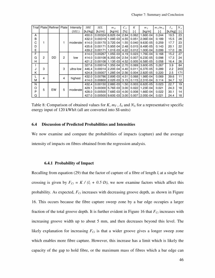
Table 8 Comparison of obtained values for K mT IA and NA for a representative specific
energy input of 120 kWht (all are converted into SI-units) 46
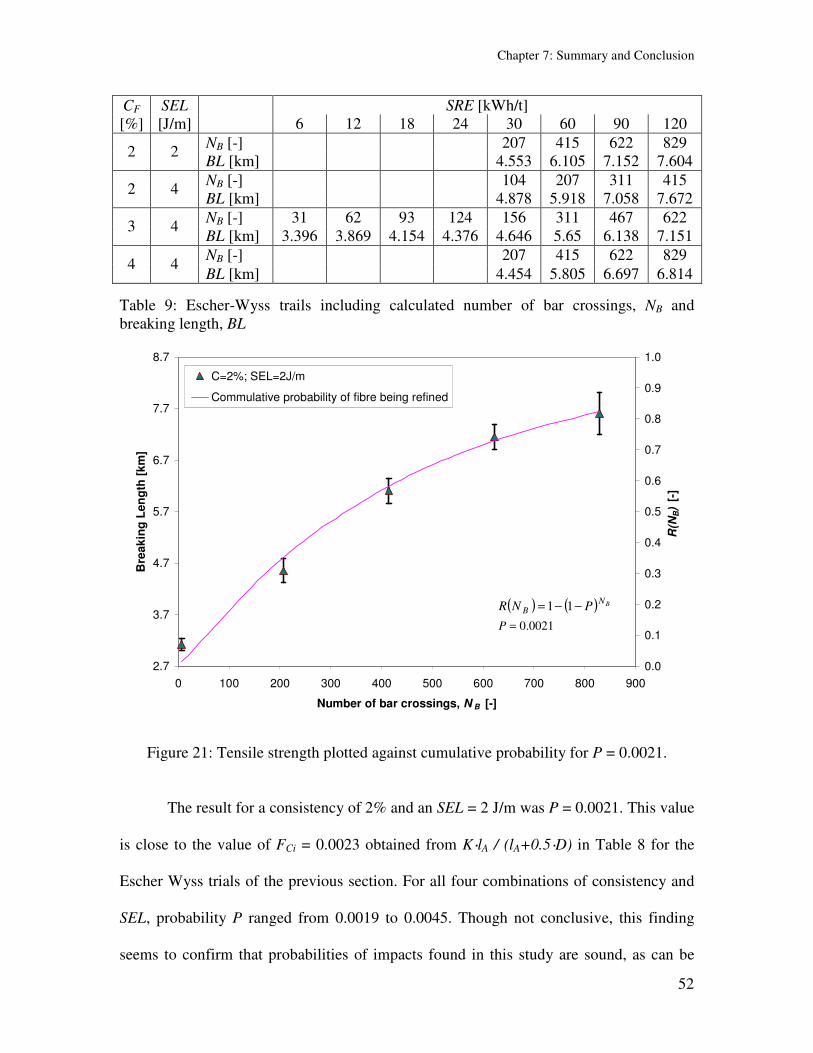
Table 9 Escher-Wyss trails including calculated number of bar crossings NB and
breaking length BL 52
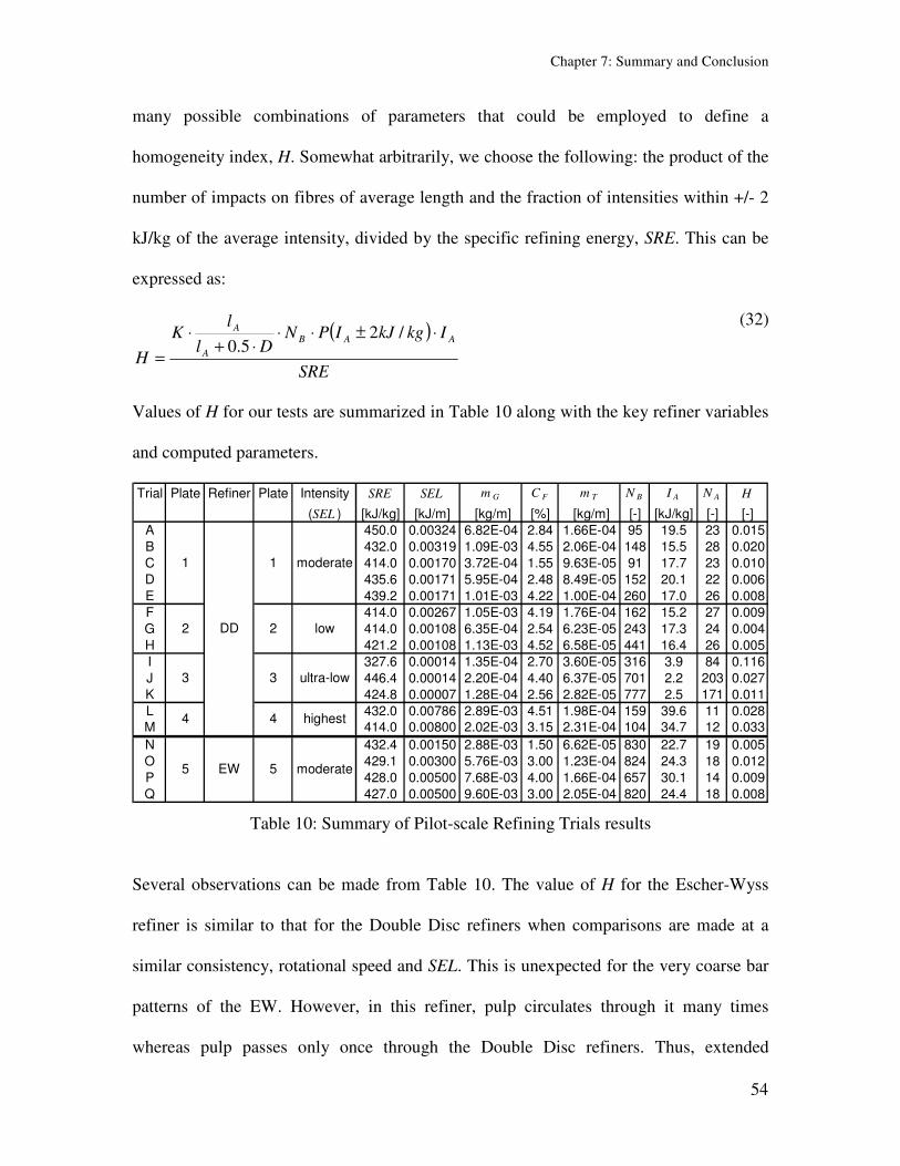
Table 10 Summary of Pilot-scale Refining Trials results 54
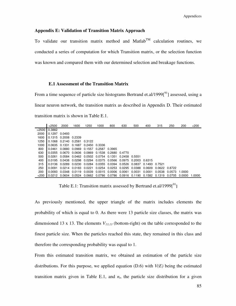
Table E1 Transition matrix assessed by Bertrand etal1999[91
] 85
Table E2 Calculated evolution of particle size distribution 86
Table E3 Assessed Transition Matrix 86
Table E4 Particle size distribution 88
Table E5 Comparison of assumed and estimated Selection Function values 88
ix
List of Figures
Figure 1 Pulp flow pattern within the refiner plate by Fox1979[39
] 8
Figure 2 Same amount of energy imparted into fibres in two ways 13
Figure 3 A representative refiner bar pattern showing bar and fibre dimensions 24
Figure 4 Plate pattern showing mass location 24
Figure 5 Probability that upon being captured the average intensity IA exceeds the
rupture strength IC of two different pulp fibres 27
Figure 6 Sprout-Waldron LC-Plate (CEL = 081328 kmrev) 31
Figure 7 12rdquo Sprout-Waldron Refiner at UBC (8rdquoinner - and 12rdquoouter diameter) 32
Figure 8 Fibre Length Distribution of tracer fibres (Douglas Fir) 33
Figure 9 Refined Douglas Fir (dark brown) and White Spruce fibres using the 12rdquo
Sprout-Waldron refiner 37
Figure 10 Comparison of the selection function probability Si for 43 mm long fibres
(White Spruce) for various trial conditions and refiners 38
Figure 11 Selection function curve for Douglas Fir and White Spruce fibre fractions after
refining at SEL = 30 Jm 39
Figure 12 The experimentally determined selection function for the EscherndashWyss refiner
trials using a single refiner plate for increasing SEL 41
Figure 13 Selection function values for 43 mm long fibres for all 15 trials 42
Figure 14 Selection function dependency on Consistency for the same plate pattern on a
Double Disc refiner (Trial A-E) for fibre length of 43 mm 43
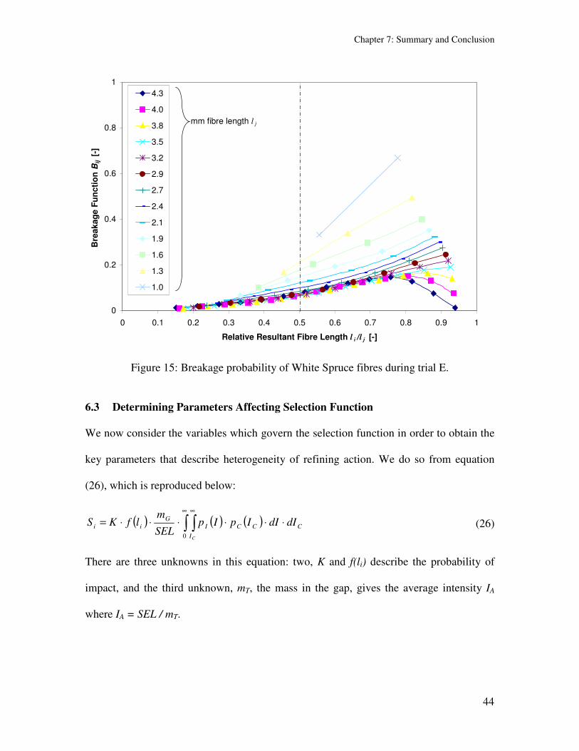
Figure 15 Breakage probability of White Spruce fibres during trial E 44
x
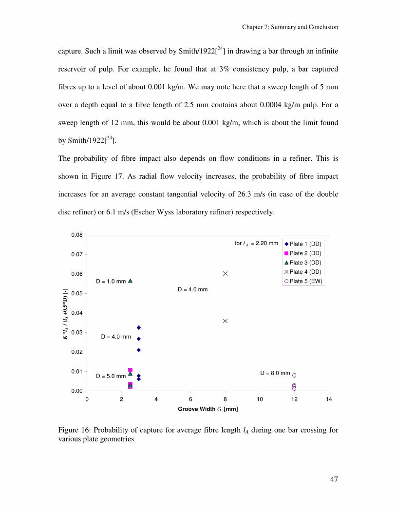
Figure 16 Probability of capture for average fibre length lA during one bar crossing for
various plate geometries 47
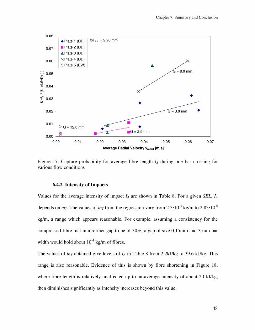
Figure 17 Capture probability for average fibre length lA during one bar crossing for
various flow conditions 48
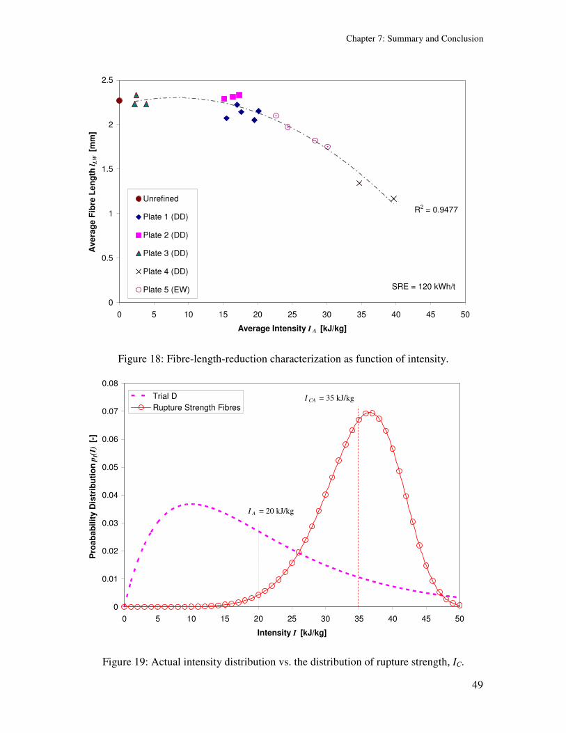
Figure 18 Fibre-length-reduction characterization as function of intensity 49
Figure 19 Actual intensity distribution vs the distribution of rupture strength IC 49
Figure 20 Comparisons of Average Intensity IA to intensity levels calculated based on
previous studies by Leider and Nissan1977[36
] and Kerekes1990[55
] 50
Figure 21 Tensile strength plotted against cumulative probability for P = 00021 52
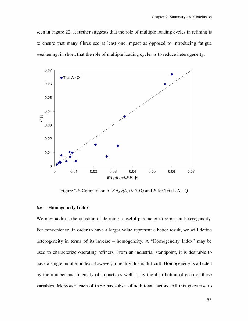
Figure 22 Comparison of KlA (lA+05D) and P for Trials A - Q 53
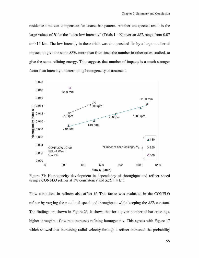
Figure 23 Homogeneity development in dependency of throughput and refiner speed
using a CONFLO refiner at 1 consistency and SEL = 4 Jm 55
Figure 24 Relationship between Tear Index and Homogeneity Index H 56
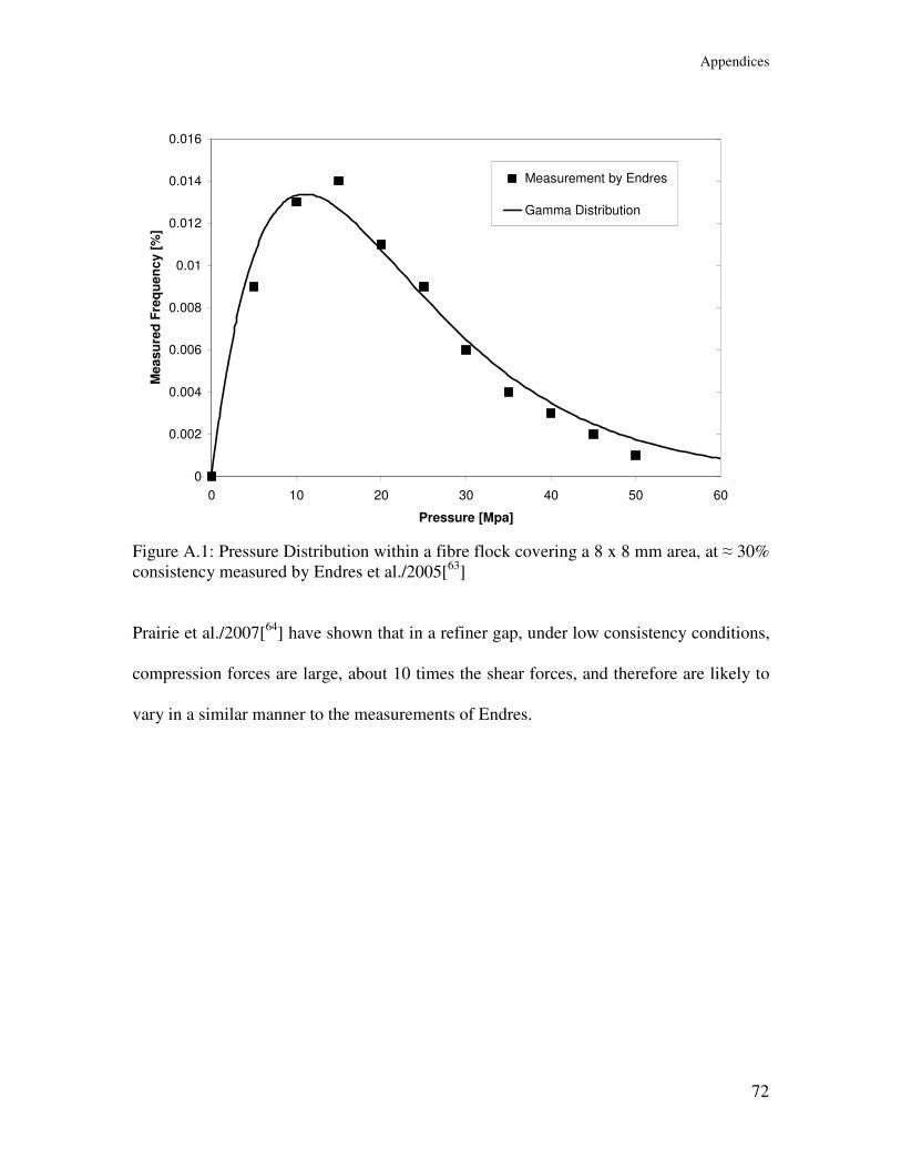
Figure A1 Pressure Distribution within a fibre flock covering a 8 x 8 mm area at asymp 30
consistency measured by Endres et al2005[63
] 72
Figure C1 Tensile strength vs fibril angle for springwood and summer wood fibre of
white spruce reproduced from Page et al1972[87
] 75
Figure C2 Frequency distribution of tensile strength for black spruce acid sulphite
fibres pulped to 63 yield at 042 and 150 span length reproduced from
Page et al1976[86
] 78
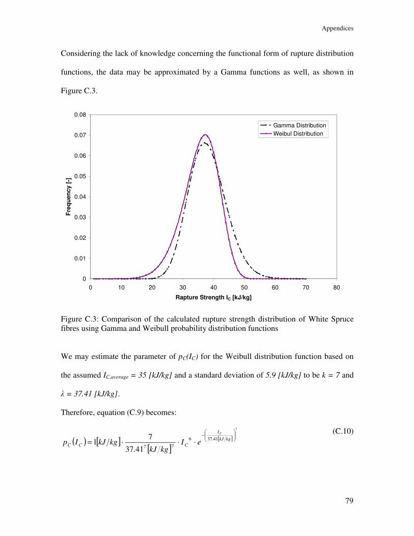
Figure C3 Comparison of the calculated rupture strength distribution of White Spruce
fibres using Gamma and Weibull probability distribution functions 79
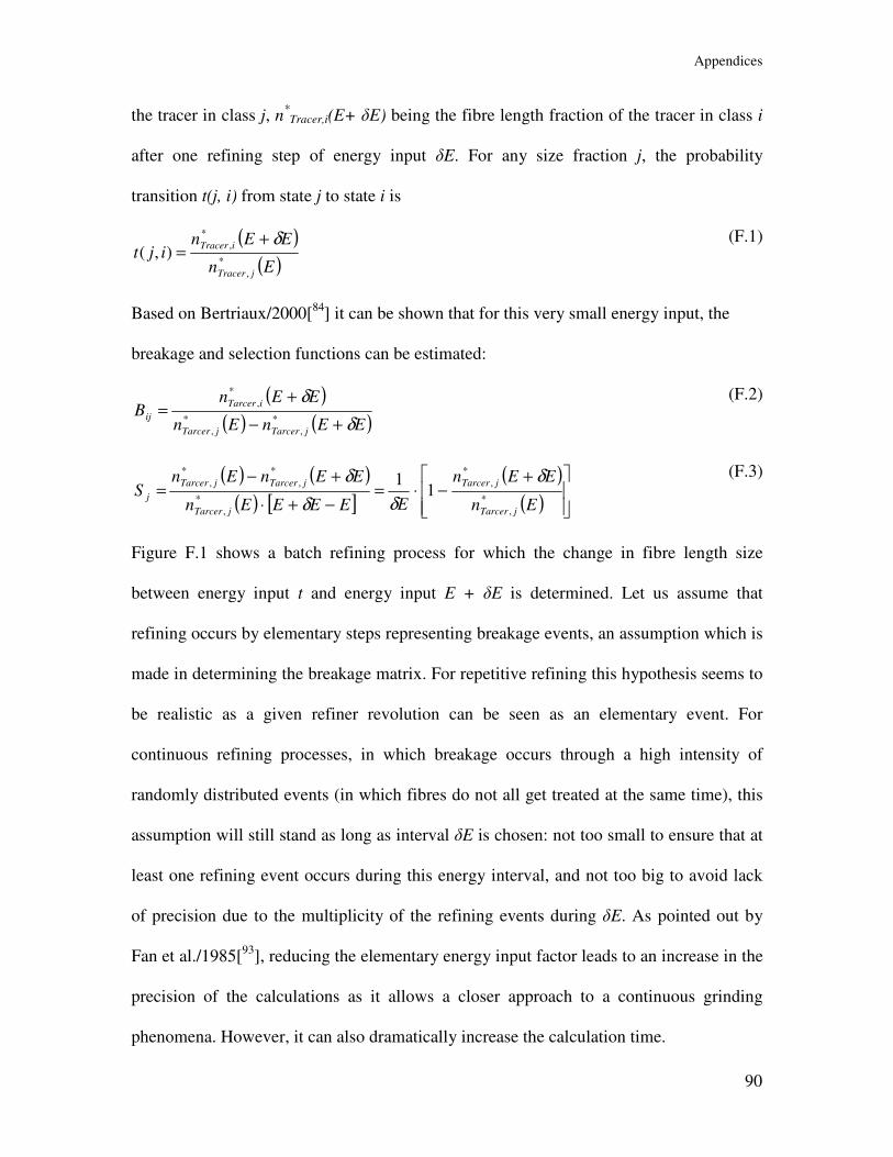
Figure F1 Stochastic Approach to Batch Refining 89
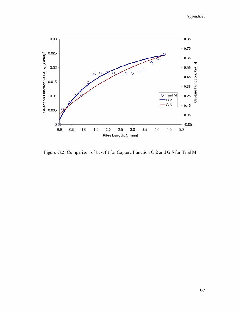
Figure G2 Comparison of best fit for Capture Function G2 and G5 for Trial M 92
xi
Nomenclature
a Shape parameter for intensity distribution [kJkg]-1
A Comminution matrix
AF Cross sectional area fibre [m2]
b Scale parameter for intensity distribution [kJkg]-1
B Breakage function matrix
Bij Breakage function [-]
BL Breaking length of paper [km]
BEL Breaking Edge Length [km]
C C-Factor [s-1
]
CF Consistency pulp suspension [] or [-]
CEL Cutting Edge Length [kms]
E Energy input [kWht]
dE Incremental energy input [kWht]
D Groove Depth [mm]
EM Elastic Modulus (Youngrsquos modulus) [Pa]
f(li) Probability of capture form of fibres of length li [-]
FCi Factor for fibres length i to be captured during one bar crossing event [-]
Fmax Maximum force [N]
G Groove width [mm]
H Homogeneity index [-]
I Intensity of impacts [kJkg]
xii
IA Average intensity of impacts [kJkg]
IC Critical rupture strength of fibres [kJkg]
ICA Average critical rupture strength of fibres [kJkg]
In Identity matrix
K Empirical constant depending on machine parameter [-]
lA Average fibre length [mm]
mamp Mass throughput of OD pulp [th] or [kgs]
mG Mass of fibres in the grooves per unit bar length [kgm]
mT Mass of fibres in the gap per unit bar length [kgm]
MEL Modified Edge Load [Jm]
n(E) Column vector of fibre length classes at energy input level E
ni Numbers of fibre length class i [-]
dnini Incremental shortening of fibres of length class i [-]
nTracerj(E) Fraction of the number of tracer fibres in length class j [-]
nt Initial state vector
N Number of impacts on fibre [-]
NA Average number of impacts [-]
NB Number of bar crossings fibre experiences while traveling thr refiner [-]
NC Number of compression cycles [-]
outi Estimated values according to Markovian transition matrix approach
P Average probability of fibre capture for one bar crossing [-]
pC(IC) Rupture strength - probability distribution density function [-]
pI(I) Intensity probability distribution density function [-]
xiii
PR Probability of refining intensity exceeding the rupture strength of fibres [-]
pGamma(I) Gamma probability distribution density function [-]
Pnet Net energy input [kW] or [kJs]
Q Volume throughput [m3s]
R1 Inner radius refiner [m]
R2 Outer radius refiner [mm]
RBA Relative Bonded Area [-]
RD(E) Matrix of eigenvalues
R(NB) Fraction of fibres that have been captured and therefore treated [-]
S Selection function matrix
Si Selection function [kWht]-1
or [kJkg]-1
SEL Specific Edge Load [Wsm] or [Jm]
SRE Specific Refining Energy [kWht] or [kJkg]
SSL Specific Surface Load [Wsm2] or [Jm
2]
t Energy state [kWht] or [kJkg]
t(j i) Probability transition matrix
TEA Tensile energy absorption [Jm2]
UT Matrix of the eigenvectors
vij Elements of V(E)
Vamp Volume flow through the refiner [m3s]
V(E) Transition matrix
w Fibre coarseness [mgm]
WR Bar Width of the Rotor [mm]
xiv
WS Bar Width of the Stator [mm]
x Number of Bins of fibre length measurement [-]
α Shape parameter for gamma distribution function [-]
αB Bar angle [deg]
β Scale parameter for gamma distribution function [-]
δE Small energy input [kJkg]
ε Elastic strain at failure [-]
θ Sector angle refiner plate [-]
k Shape parameter for Weibull probability distribution function [-]
λ Scale parameter for Weibull probability distribution function [-]
micro Learning rate parameter
ρ Density fibre [kgm3]
σ Stress (tensile strength) [Nm2] or [Pa] or [10
1 dynecm
2]
υ Poisson ratio [-]
φ Bar angle [deg]
ω Rotational speed [revmin] or [revs]
xv
Acknowledgments
I would like to thank my supervisors James Olson and Richard Kerekes for providing
strong leadership inspiration and support over the course of my PhD and for showing
me what it takes to bring an academic quest through to completion I would also like to
thank my committee members Mark Martinez and Chad Bennington for their help and
advice in this project I wish also to acknowledge my co-researchers and staff of the pulp
and paper centre at UBC for their work ethic and encouragement namely Sean Delfel
Paul Krochak Tim Paterson and Ken Wong
It was absolutely necessary to have a supportive network of friends and family to help me
on my journey through this project My deepest thanks to those in my life who always
supported and encouraged me over the past years
Grateful acknowledgement is made for financial and technical support from NSERC
CANFOR STORA ENSO and FPInnovations Paprican Division
Chapter 1 Introduction
1
1 Introduction
Pulp refining is one of the most important unit operations in papermaking Its purpose is
to modify fibre morphology in order to improve paper properties by a technology which
has developed from batch beaters in the early 19th
century to flow-through disc conical
and cylindrical refiners in use today In pulp refiners fibres are trapped in the gaps
between bars during bar crossings during pulp flow through an annulus between a rotor
and stator which have bars on their surfaces and subjected to cyclic compression and
shear forces which modify fibre properties
The result of refining is changes in physical and optical properties of paper have been
studied in detail by various authors over the past decades (Higgins and de Yong1962[1]
Page1985[2] Seth1996[
3] and Hiltunen et al2002[
4]) to name only a few) It has been
generally found that within the commercial range refining increases tensile strength
(about threefold) burst strength folding endurance and sheet density whereas it reduces
tear strength of paper and sometimes fibre length
Although there is extensive literature on changes in fiber morphology produced by
refining there is relatively little on how the refining action takes place that is on the
refining process itself (Atack1980[5] Page1989[
6]) Consequently quantitative
characterization of refining action is limited The most widely used quantitative measure
of refining action is net energy expended per unit mass ie specific refining energy
(SRE) In addition it is common to use a ldquorefining intensityrdquo which reflects the energy
expended per loading cycle at each bar crossing event However although useful energy-
based characterizations have limitations because most changes within fibres occur as a
Chapter 1 Introduction
2
result of forces not energy The use of force in characterizing refining action has only
recently been undertaken (Kerekes and Senger2006[46
])
It has long been known that refining is very non-uniform in its treatment of pulp
(Danforth1986[7]) However the causes and consequences of this heterogeneity have
been little studied Furthermore heterogeneity of treatment has not been taken into
account in any of the refining theories or characterizations due in good part to a lack of
means to measure heterogeneity Thus it is reasonable to expect that a better
understanding of the nature of heterogeneity in refining will lead to a better
understanding of the process and perhaps offer a basis for improved technology
The objective of this dissertation is to develop a method to measure heterogeneity of
treatment in operating refiners
Chapter 2 Review of Literature
3
2 Review of Literature
Several excellent reviews of pulp refining have been produced over the years Generally
they have emphasized changes in fibre morphology caused by refining for example
Higgins and de Yong1962[1] Page et al1962[
8] Atack1977[
9] Page1985[
2]
Seth1996[3] and Hiltunen et al2002[
4]) The fundamentals of the refining process have
also received study as shown in the reviews of Ebeling1980[10
] Page1989[6]
Hietanen1990[11
] and Hietanen and Ebeling1990[12
]) The following review of the
literature will focus on highlights from past studies relevant to heterogeneity of treatment
21 Effect on Pulp
The main effects of refining on pulp are internal fibrillation external fibrillation fibre
shortening and fines generation More recently fibre straightening has been recognized as
another primary effect by Page1985[2] Mohlin and Miller1995[
13] and Seth2006[
14]
These outcomes of refining are described below in more detail
211 Internal Fibrillation
Measurements by Mohlin1975[15
] Kerekes1985[16
] and Paavilainen1993[17
] have
shown that refining chemical pulp increases fibre flexibility This occurs from
delamination in the cell wall which lowers its effective elasticity Water is drawn into the
fibre walls by capillary forces causing swelling which is often used as an indicator of
degree of refining The weakened cell wall is more flexible and collapsible thereby
giving a larger relative bonded area in paper This in turn increases bonding and thereby
paper strength
Chapter 2 Review of Literature
4
212 External Fibrillation
Another effect in commercial refining is the delamination of fibre surfaces called
external fibrillation This can be defined as a peeling off of fibrils from the fiber surface
while leaving them attached to the fiber surface (Page et al1967[18
] Page1989[6])
Clark1969[19
] emphasized that the fiber surface can be fibrillated even in the early
beating stage and that the external fibrils serve as bonding agents for inter-fiber bonding
The amount of such fibrillation (parts of fibre wall still attached to fibre) can be
quantified by measuring the increase in the specific surface of the long fibre fraction
(Page1989[6]) Although external fibrillation was studied from the earliest years of
refining because it was easily observable under microscope and was thought to be the
dominant result of refining several modern authors ie Page1985[2] and
Hartman1985[20
] concluded that external fibrillation has only limited effect on the tensile
strength or elastic modulus
213 Fibre Shortening
Refining causes fibre shortening which is generally undesirable in refining In some rare
applications it is a desired effect to improve formation by decreasing the crowding
number (Kerekes1995[21
]) In early work Page1989[6] showed that the mode of fibre
shortening was tensile failure rather than ldquocuttingrdquo by scissor-like shearing
214 Fines Generation
Fines meaning loose fibrous material of size less than 03 mm are produced in refining
as a result of fibre shortening or removal of fibrils from fibre walls According to
Chapter 2 Review of Literature
5
Page1989[6] generated fines consist mostly of fragments of P1 and S1 layers of the fibre
wall due to the abrasion of fibres against each other or against refiner bars
215 Fibre Straightening
Fibre straightening is considered an important refining effect (Page1985[2]
Mohlin1991[22
] Seth2001[23
]) If fibres remain curly or kinked in a paper network they
must be stretched before they can carry load meaning that fewer fibres carry load during
the initial stretching of paper and therefore paper is weak Fibre straightening permits
fibre segments between bonded sites in paper to be ldquoactiverdquo in carrying load The
mechanism by which refiners straighten fibres is likely due in part to tensile strain in
refiner gaps and by causing fibre diameter swelling In the latter case upon drying
shrinkage of swollen fibres stretches fibres segments between bonded sites and thereby
straightens them
216 Heterogeneity
It has long been known that refining is a heterogeneous process and that the resulting
heterogeneity affects paper properties One of the earliest workers to show this was
Danforth1986[7] by mixing of fibres subjected to differing levels of refining Larger
heterogeneity gave poorer properties eg lower tensile strength Others have shown
heterogeneity by observations of morphology changes (Page1989[6]) The literature on
heterogeneity will be reviewed extensively later in section 26
22 Mechanics of Refining
Current knowledge of the mechanics of refining is far less than is knowledge of the
refining result The design of refiners is largely empirical In addition to action on pulp
Chapter 2 Review of Literature
6
design is based on factors such as sufficient groove size to permit flow of the fibre
suspension through the machine bar wear and material cost Scientific studies of the
process of refining have been carried out by various researchers Some highlights of this
past work are described below
221 Fibrage Theory
Smith1922[24
] proposed that a refiner bar moving through stock collects a ldquobeardrdquo or
fibrage of fibers on the leading edge This capture of fibre transports fibres into the gap
between rotor and stator bars A study of the compressive and shearing forces exerted on
the bars during refining by Goncharov1971[33
] gave some support to the fibrage
mechanism
222 Refining as Lubrication Process (Hydrodynamics)
Rance1951[25
] and Steenberg1951[26
] analyzed refining as a lubrication process Their
experiments offered indirect evidence of the occurrence of (a) fluid (hydrodynamic)
lubrication (b) boundary lubrication and (c) lubrication breakdown which produced
excessive metal wear in the refiner Steenberg1951[26
] carried out his experiments with a
Valley beater varying the consistency load and peripheral speed He concluded that
Valley beating is carried out under hydrodynamic (fluid) lubrication conditions and that
the work absorption capacity ie coefficient of friction decreases with beating as does
the apparent viscosity of the pulp More recently Frazier1988[27
] applied the lubrication
theory to refiner mechanical pulping and derived an expression for the shear force applied
to pulp Similarly Roux1997[28
] performed a lubrication analysis in order to characterize
hydrodynamic forces in refining Based on experiments Lundin et al1999[29
] propose
Chapter 2 Review of Literature
7
that the power consumption in refining is governed by a lubrication film between the
rotor and the stator Although characterization of the refining process as a hydrodynamic
phenomenon has yielded some useful correlations treating the fibre suspension as a fluid
has some serious limitations Refiner gaps are 5-10 fibre diameters deep and therefore the
water-fibre suspension in a gap is not a continuum Consequently the suspension in the
gap does not meet a primary property of a fluid
223 Transport Phenomena in Refiners
Flow behavior in refiners has been examined by several workers Complex flow patterns
have been observed and residence time distributions have been measured using high
speed photography (Halme and Syrjanen1964[30
] Herbert and Marsh1968[31
]
Banks1967[32
] Gonchorov1971[33
] Fox et al1979[34
] and Ebeling1980[10
]) Halme
and Syrjanen1964[30
] Herbert and Marsh1968[31
] observed that pulp flows primarily in
the radial direction outward in the grooves of the rotor and inward in the grooves of the
stator Other recirculation flows called secondary and tertiary flows are also present in
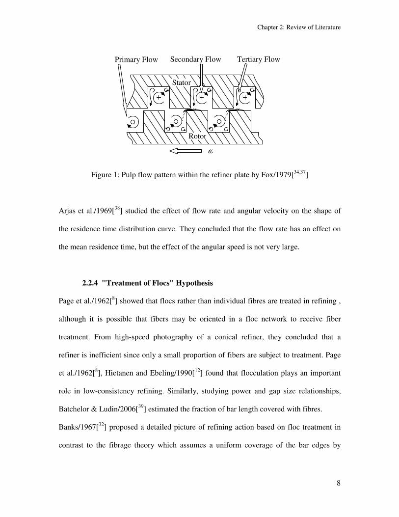
disc refiners Fox et al[34
] proposed that the secondary flows arise from the motion of the
land area of the bars passing over the grooves and that tertiary flows result from the
difference in static pressure between opposing grooves of the rotor and stator (see Figure
1) Using a material and energy balance Leider and Rihs1977[35
] and Leider and
Nissan1977[36
] related the pressure drop across the refiner to its volumetric flow rate
This accounts for the action of the centrifugal and frictional forces and is expressed in
terms of operating conditions fluid properties and plate properties
Chapter 2 Review of Literature
8
Figure 1 Pulp flow pattern within the refiner plate by Fox1979[3437
]
Arjas et al1969[38
] studied the effect of flow rate and angular velocity on the shape of
the residence time distribution curve They concluded that the flow rate has an effect on
the mean residence time but the effect of the angular speed is not very large
224 Treatment of Flocs Hypothesis
Page et al1962[8] showed that flocs rather than individual fibres are treated in refining
although it is possible that fibers may be oriented in a floc network to receive fiber
treatment From high-speed photography of a conical refiner they concluded that a
refiner is inefficient since only a small proportion of fibers are subject to treatment Page
et al1962[8] Hietanen and Ebeling1990[
12] found that flocculation plays an important
role in low-consistency refining Similarly studying power and gap size relationships
Batchelor amp Ludin2006[39
] estimated the fraction of bar length covered with fibres
Banks1967[32
] proposed a detailed picture of refining action based on floc treatment in
contrast to the fibrage theory which assumes a uniform coverage of the bar edges by
Tertiary Flow
Rotor
Stator
ω
Primary Flow Secondary Flow
Chapter 2 Review of Literature
9
individual fibres He summarized the mechanics of refining based on observations using
high-speed photography
1 Flocs consolidate when they are trapped between approaching tackle elements
2 Mechanical pressure induced by the tackle elements becomes high enough and
causes plastic deformation in the fibers composing the floc Consolidation
continues
3 The floc compressed between the bars is sheared flocs (and fibers) are
ruptured
4 Release of mechanical pressure allows absorption of water to take place into
the ruptured fibrils and fibers
5 Turbulent agitation may disperse the floc or its remnants into the general mass
flow
225 Refining as a Fatigue Process
Fibres may be exposed to many bar crossing events during their passage through a
refiner Thus fibres are likely to experience multiple loading cycles Page et al1962[8]
and Atack1977[9] suggested that this repeated straining causes fatigue weakening of the
fibres and this in turn produces internal fibrillation On the other hand fibre shortening
(cutting) is likely to be caused by one severe loading cycle Page1989[6] suggested
rupture takes place by tensile failure rather then a scissor-like cutting action Kerekes and
Olson2003[40
] proposed that fibre rupture in refiners is caused by a single event rather
than fatigue process
Another approach to account for the cyclical nature of the process was proposed by
Steenberg1979[41
] He considered the refining process to be an irreversible kappa
Chapter 2 Review of Literature
10
process in which there is a critical path for the formation of a stress concentration chain
which causes a structural breakdown For another structural breakdown to occur the
particles ie fibers need to be rearranged Thus cyclicality is needed to overcome
heterogeneity Most recently Goosen et al2007[42
] examined the role of fibre
redistribution in pulp refining by compression They concluded that the role of cyclic
loading is to expose new fibres to loading cycles rather than to produce fatigue
weakening In essence cyclicality in the process is to overcome heterogeneity rather then
to produce fatigue weakening
226 Forces on Fibres during Bar Crossing Events
A number of studies have examined the manner in which forces are imposed on fibres
within refiner gaps Page 1989[6] suggested that refining should be quantified by the
stresses and strains applied to fibres These stresses and strains are caused by bar forces
which have been the subjects of several studies
Goncharov1971[43
] was the first to measure pressures on refiner bars during bar crossing
events Later Martinez et al1997[44
] and Batchelor et al1997[45
] analyzed the
compressive and shear forces action on single flocs and measured normal and shear
forces in a ldquosingle barrdquo refiner apparatus Kerekes and Senger[46
] developed equations
for bar forces and fibre forces from the specific edge load (SEL) Page1989[6] Martinez
et al1997[44
] and Koskenhely et al2007[47
] addressed issues concerning the bar edge
force
Chapter 2 Review of Literature
11
23 Quantitative Characterization of the Refining Mechanism
As described earlier specific refining energy is the most common quantitative
characterization of refining action This energy is factored into the number of impacts
imposed on pulp and the intensity of each impact ie loading cycle Most intensities are
based on energy per loading cycle though in recent work Kerekes and Senger2006[46
]
have proposed a force-based intensity These concepts are described in detail below
231 Specific Energy
Specific refining energy (SRE) is the useful energy imparted to the pulp suspension ie
the total energy less the no-load energy It is obtained by dividing the net power input
into the refiner by the fibre mass throughput
ρsdotsdot==
VC
P
m
PSRE
F
netnet
ampamp
(1)
The typical range for SRE in chemical pulp refining is between 80 to 250 kWht
depending on the furnish and the desired papermaking property
232 Refining Intensity
The major means of characterizing refining intensity today is by a ldquomachine intensityrdquo
meaning an intensity which reflects energy expended per bar crossing without direct
reference to how this energy is expended pulp The most common such method is the
Specific Edge Load (SEL) This was introduced by Wultsch and Flucher1958[48
] and
developed further by Brecht and Siewert1966[49
] who demonstrated the dominant impact
of the bar edge The SEL is determined by the net power divided by the bar edge length
(BEL) multiplied by the rotational speed ω The BEL is determined by multiplying the
Chapter 2 Review of Literature
12
number of bars on stator by the number of bars on rotor by the refining zone length The
result is expressed in Wsm or Jm The expression for SEL is
CEL
P
BEL
PSEL netnet =
sdot=
ω
(2)
int sum∆sdot
congsdotsdot
=2
11 coscos
R
R
Nsrsr rnnrnn
BELθθ
(3)
An extension of the SEL the specific surface load (SSL) was suggested by
Lumiainen1990[50
] to account for bar width rather than just bar edges This was
accomplished by including bar width W with the SEL thereby giving the area of the bars
and units Wsm2 or Jm
2
( )
sdot
+sdotsdot
=
2cos2 B
SR
net
WWCEL
PSSL
αω
(4)
Using this approach Lumiainen distinguished between refiner plates having identical
cutting edge length (CEL) but differing bar widths
Meltzer and Rautenbach1994[51
] used the ldquocrossing speedrdquo ndash which is a measure of fibre
treatment frequency by calculating the crossing speed per dry fibre mass flow ndash to further
modify the SEL-concept This gave the modified edge load (MEL) which accounts for bar
width W groove width G and the average intersecting angle of rotor and stator bars For
identical rotor and stator geometry the following expression was derived
W
GWSELMEL
B
+sdot
sdotsdot=
αtan2
1
(5)
The factor W+G W considers the refining work of the bar surfaces and the probability of
fibre treatment received
Chapter 2 Review of Literature
13
233 Fibre Intensity
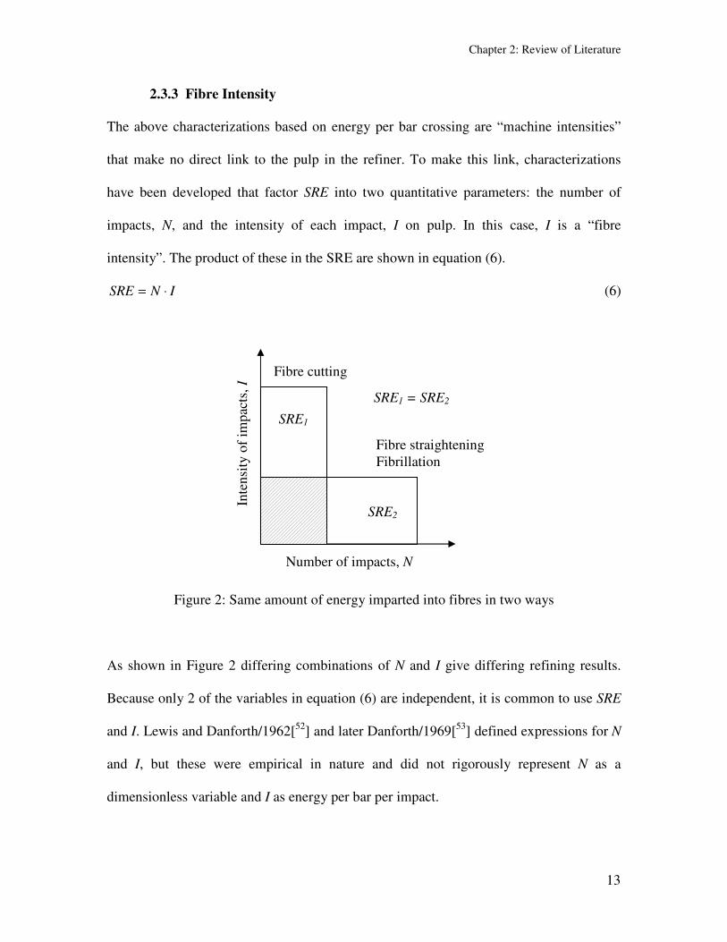
The above characterizations based on energy per bar crossing are ldquomachine intensitiesrdquo
that make no direct link to the pulp in the refiner To make this link characterizations
have been developed that factor SRE into two quantitative parameters the number of
impacts N and the intensity of each impact I on pulp In this case I is a ldquofibre
intensityrdquo The product of these in the SRE are shown in equation (6)
INSRE sdot= (6)
Figure 2 Same amount of energy imparted into fibres in two ways
As shown in Figure 2 differing combinations of N and I give differing refining results
Because only 2 of the variables in equation (6) are independent it is common to use SRE
and I Lewis and Danforth1962[52
] and later Danforth1969[53
] defined expressions for N
and I but these were empirical in nature and did not rigorously represent N as a
dimensionless variable and I as energy per bar per impact
Number of impacts N
Inte
nsi
ty o
f im
pac
ts
I
Fibre cutting
Fibre straightening
Fibrillation
SRE1 = SRE2
SRE1
SRE2
Chapter 2 Review of Literature
14
Van Stiphout1964[54
] calculated the probability of a fibre being caught in the refiner gap
Based on this he was able to estimate the forces acting on fibres and the mass of fibres
being treated per length of bar According to his analysis the mass of fibres per bar length
was proportional to the mean residence time He further postulated that the damaging
affect of refining was proportional to the surface sheared and that the net power was
active on an amount of fibres enclosed in the gap between the refiner bars However two
empirical parameters of unknown magnitude limited the application and scientific
meaning of this work
Leider and Nissan1977[36
] were the first to derive equations for N and I in rigorous
terms They represented the probability of a fibre being stapled on a bar by fibre length
and diameter to give an estimate of ldquonumber of impacts per single fibre per refiner passrdquo
Another approach to define values for N and I to overcome some of the shortcomings of
Leider and Nissan was made by Kerekes1990[55
] in the form of the C-factor
C
P
m
CIN
m
PSRE netnet sdot=sdot==
ampamp
(7)
In this approach C is defined as the capacity of a refiner to inflict impacts (loading
cycles) on fibres Kerekes1990[55
] derived equations for the C-factor as a function of
plate geometry (bar width depth length angle and edge geometry) speed consistency
fiber length and coarseness The C-factor for a disc refiner for a simplified case (small
gap size similar bar pattern on rotor and stator) is given by
( )( )( )Dlw
RRnlCGDC
A
AF
+
minus+sdot=
3
tan218 3
1
3
2
32 φωρπ
(8)
A crucial assumption of the analysis is estimating the probability of fiber contact with the
leading edge of the bar which he expresses as l (l + D+ T) Kerekes showed that this
Chapter 2 Review of Literature
15
assumption led to logical outcomes at the limits of bar size relative to fibre length The C-
Factor analysis is perhaps the most rigorous and comprehensive theory developed to date
It has been applied to a variety of refiner geometries including the disk conical and PFI
mill It takes into account factors relating to bar and groove geometry as well as fibre
length which provide a more accurate description of refining intensity However the C-
factor predicts only average values rather than distributions of intensity
24 Heterogeneity
It has long been accepted that refining is a heterogeneous process (Page1989[6]) The
sources of heterogeneity are numerous ranging from the mechanism of transferring
mechanical forces into fibers (Steenberg1963[56
]) to the irregular flow pattern through
the refiner (Halme1962[57
])
There are also scales of heterogeneity ranging from large to small Ryti and
Arjas1969[58
] studied the large distributions of residence time in refiners originating
from large scale secondary flows They postulated that greater uniformity in refining
treatment gives a better refining result They concluded that the refining action is related
to the residence time inside the refiner and to the probability of treatment during this
time Fox et al1979[34
] studied flow in a small disc refiner by visual observation They
found that after being ldquoreleasedrdquo from a gap fibres either become part of the stator flow
towards the refiner axis and stapled again on a bar or become part of the outward rotor
flow leaving the refiner In addition fibres may flow back to the stator from the outside
annulus of the refiner This all resulted in a poor pulp circulation and therefore limited the
amount of fibres receiving treatment in refiner gaps
Chapter 2 Review of Literature
16
Additional sources of heterogeneity arise from a finite probability of capture from the
groove (Olson et al2003[59
]) fractional bar coverage (Batchelor and Ludin2006[60
])
non-uniform force distribution within flocs (Batchelor and Ouellet1997[61
]) non-
uniform SEL along the radius of the refiner (Roux and Joris2005[62
]) non-homogeneous
force distribution on fibre networks while being under load (Endres et al2005[63
]) and
out-of-tram of rotors (Prairie et al 2007[64
]) An added complexity is the wide variability
of fibre properties in any pulp It is well known that species pulp type bleaching process
and the relative amounts of thick and thin walled fibers can affect refining Page1983[65
]
has suggested that differences in the beatability and refining action of kraft and sulfite
pulps are due to differences in their viscoelastic behavior Yet another factor is fibre
flocculation Hietanen and Ebeling1990[12
] Hietanen1991[66
] and Lumiainen1995[67
]
have all suggested that flocculation is a major source of refining heterogeneity
Various studies have been conducted to measure heterogeneity of treatment in refining
Simons1950[68
]) used a staining technique to identify damaged fibres Nisser and Brecht
1963[69
] evaluated refining heterogeneity by calculating the swollen length of fibres
before and after refining Another approach has been to examine physical changes in
fibres Mohlin and Librandt1980[70
] using SEM technique found that one of the major
differences between laboratory refining and production refining is the homogeneity of
treatment Dahrni and Kerekes1997[71
] measured deformations in plastic tracer fibres
They found that 30 of the fibre passed through a lab disc refiner with no visible sign of
impact whereas other fibres were severely deformed Dekker2005[72
] measured the
changes in RBA of fibres by quantifying the optical contact between fibres and a glass
slide He found that only 7-20 of fibres were treated
Chapter 2 Review of Literature
17
Another approach for measuring heterogeneity is based on comparing properties of
papers made from mixtures of unrefined and well-refined pulp (Dillen1980[73
]) As a
measure of the heterogeneity he used the coefficient of variation of the amount of
refining Lastly Hietanen1991[66
] found that the homogenizing effect of deflocculation
has a positive impact on paper strength properties
In summary the sources of heterogeneity in refining are many and there are some
methods to measure it but no existing methods are suitable for measurement of
heterogeneity of treatment in operating refiners
25 Review of Refining Action as a Comminution Process
Comminution is defined as the reduction of particle size by mechanical processing
Models for the comminution process models were developed for crushing and grinding in
the powder industry 60 years ago to predict particle size distribution changes during
processing The basics were developed by Epstein1948[74
] Reid1965[75
] and
Austin1971[76
] They modeled batch grinding by the introduction of two statistical
functions a Breakage function Bij and a Selection function Si Basically Si represents
the probability of a particle of size i per unit time or energy and has the units of time-1
or
energy-1
The breakage function Bij represents the probability of particles larger than i
being reduced to size i As the particle size can only be reduced during grinding the
values of Bij are dimensionless and range between 0 and 1
The incremental change in the number of fibres of length i dni per incremental applied
energy dE is given by the comminution equation shown below
Chapter 2 Review of Literature
18
jj
ij
ijii
i nSBnSdE
dnsum
gt
+minus= (9)
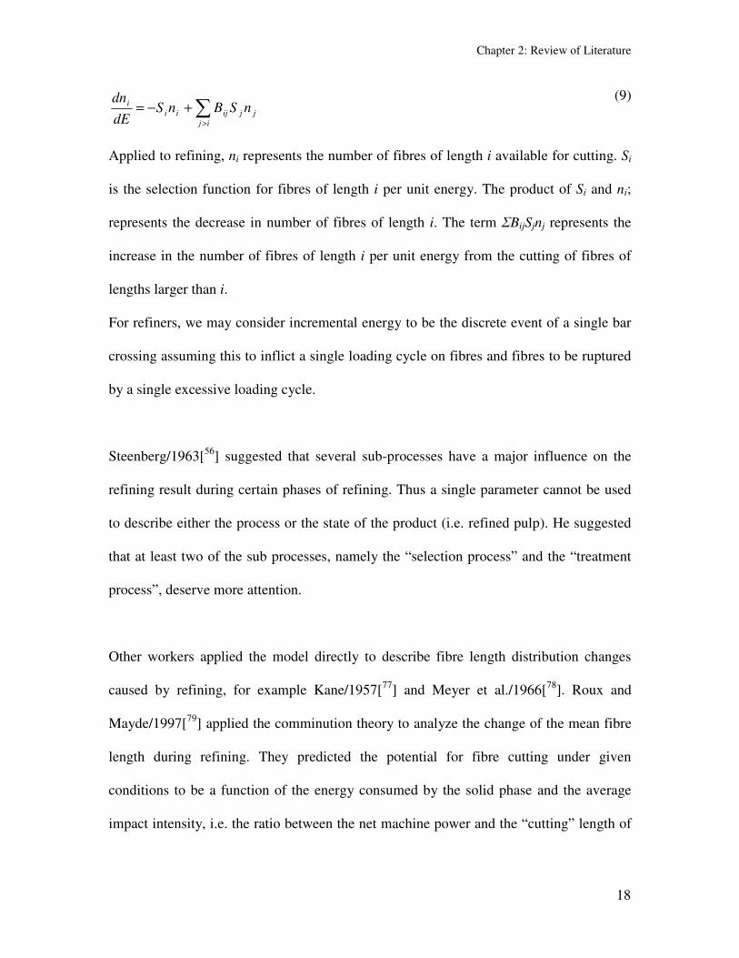
Applied to refining ni represents the number of fibres of length i available for cutting Si
is the selection function for fibres of length i per unit energy The product of Si and ni
represents the decrease in number of fibres of length i The term ΣBijSjnj represents the
increase in the number of fibres of length i per unit energy from the cutting of fibres of
lengths larger than i
For refiners we may consider incremental energy to be the discrete event of a single bar
crossing assuming this to inflict a single loading cycle on fibres and fibres to be ruptured
by a single excessive loading cycle
Steenberg1963[56
] suggested that several sub-processes have a major influence on the
refining result during certain phases of refining Thus a single parameter cannot be used
to describe either the process or the state of the product (ie refined pulp) He suggested
that at least two of the sub processes namely the ldquoselection processrdquo and the ldquotreatment
processrdquo deserve more attention
Other workers applied the model directly to describe fibre length distribution changes
caused by refining for example Kane1957[77
] and Meyer et al1966[78
] Roux and
Mayde1997[79
] applied the comminution theory to analyze the change of the mean fibre
length during refining They predicted the potential for fibre cutting under given
conditions to be a function of the energy consumed by the solid phase and the average
impact intensity ie the ratio between the net machine power and the ldquocuttingrdquo length of
Chapter 2 Review of Literature
19
bars per unit time However their equations had inconsistent units making their results
difficult to interpret rigorously
Corte and Agg1980[80
] used a comminution model to compare the shortening rate of
fibres in a disc refiner and a laboratory beater They found that the disc refiners cut long
fibre more rapidly than short fibres while a laboratory beater cut long and short fibres at
the same rate Olson et al2003[59
] applying a technique developed by Koka and
Trass1988[81
] found that the probability of fibres being selected for cutting during
refining is proportional to the applied energy and fibre length and was independent of
consistency Regression fitting that minimizes the difference between measured and
predicted fibre length distributions was used to determine the selection function Si for
various pulp and refiner combinations
Several other investigators applied the comminution theory to the production of
mechanical pulp in chip refiners Corson1972[82
] modeled the refining of wood chips
into individual fibres using a comminution approach This approach was used more
recently in an expanded form by Strand and Mokvist1989[83
] to model the operation of a
chip refiner employed in mechanical pulping of wood chips
Chapter 3 Objective of Thesis
20
3 Objective of Thesis
The above review shows that there is a need for a rigorous practical method to measure
heterogeneity in operating refiners The objective of this thesis is to develop such a
method The approach is based on interpreting measurements of fibre shortening by a
model of the physical process of refining described by comminution theory
Chapter 4 Analysis
21
4 Analysis
Comminution modeling is a potentially useful basis for measuring heterogeneity for
several reasons Fibre shortening obviously reflects the probabilistic nature of refining
because some fibres are shortened while others are not The result decreased fibre length
is a measurable change for which instruments for rapid measurement are now available
Lastly the best tracer particles to reflect what happens to fibres are fibres themselves
Fibre shortening is generally not an objective of refining Indeed it is to be avoided in
most cases In this study fibre shortening will be used merely as an event to characterize
the mechanics of the process rather that as a desired outcome We employ comminution
theory as the scientific basis of our approach To do so we address several individual
problems
interpretation of comminution equation
link to refiner mechanics
probability of fibre capture in a gap
probability of fibre shortening in a gap
link between breakage function and selection function
Chapter 4 Analysis
22
41 Interpretation of Comminution Equation
As discussed earlier the comminution equation reflects the net change in the number of
fibres of size i as the result of the decrease size i caused by shortening and the increase
caused by fibre shortening from larger sizes
jj
ij
ijii
i nSBnSdE
dnsum
gt
+minus= (10)
However our specific interest in this work is only the shortening component of
comminution Therefore we focus on the first two terms of the comminution equation
We define the incremental shortening as dni to differentiate it from the net shortening
dni in equation (10) Rearranging terms we obtain
dESn
dni
i
i sdotminus=
(11)
In essence this equation relates the incremental fraction of fibres of length i (dni ni)
that are shortened to the product of the selection function Si and the incremental energy
supplied dE
We now consider SidE in terms of refiner variables specifically to fibre rupture during a
single bar crossing The probability of fibre rupture is the product of two other
probabilities a factor of fibre capture from the groove FCi and the probability that once
captured the fibre is ruptured PR We consider PR the probability that the intensity a
fibre sees is greater than its rupture strength (intensity) to be independent of fibre length
Thus we may express SidE as
RCii PFdES sdot=sdot (12)
We now link dE FCi and PR to refiner mechanics and thereby refiner variables
Chapter 4 Analysis
23
42 Link to Refiner Mechanics
We first link energy per mass supplied to a refiner E to the product of number of impacts
imposed on fibres N and the intensity per input I expressed as energy per mass
INE sdot= (13)
We may express this equation in incremental form as
dNIdINdE sdot+sdot= (14)
Assuming that for a given refiner the average intensity at bar crossings is constant and
represented by IA and since dI = 0 we obtain
dNIdE A sdot= (15)
421 Intensity
We now interpret N and IA in terms of measurable refiner variables at a single bar
crossing
Refining intensity is commonly defined by the Specific Edge Load (SEL) Kerekes and
Senger2006[46
] have shown that SEL represents the energy expended per bar crossing
per unit bar length Thus the average energy expended on fibre mass within the gap of a
bar crossing IA is given by SEL divided by the mass of fibres in the gap per unit bar
length mT ie
T
Am
SELI =
(16)
422 Number of Impacts
The number of impacts on pulp N is a function of the product of two factors the
probability of an impact at a single bar crossing and the number of bar crossings NB that a
Chapter 4 Analysis
24
fibre would experience if it passed along a stator bar during its residence time in the
refiner We can define a mass-average probability of impact at a bar crossing by the ratio
of the mass of pulp captured mT to the total mass associated with a bar crossing (pulp in
gap and pulp in adjacent groove mG) giving mT (mT + mG) Thus
( ) BGTT dNmmmdN sdot+= (17)
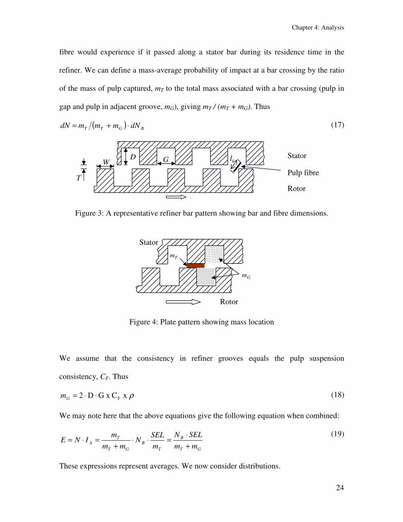
Figure 3 A representative refiner bar pattern showing bar and fibre dimensions
Figure 4 Plate pattern showing mass location
We assume that the consistency in refiner grooves equals the pulp suspension
consistency CF Thus
ρ x CG x D2 Fsdotsdot=Gm (18)
We may note here that the above equations give the following equation when combined
GT
B
T
B
GT
T
Amm
SELN
m
SELN
mm
mINE
+
sdot=sdotsdot
+=sdot=
(19)
These expressions represent averages We now consider distributions
Rotor
Stator
Tm
Gm
G D W
T Pulp fibre
Stator
Rotor
li
Chapter 4 Analysis
25
43 Fibre Capture Factor
The above mass-average probability of capture assumes a dependence only on mass ratio
However other factors also affect fibre capture For example the mass in a groove may
not reflect eligible fibres because there may be dead zones of inactive fibres stuck in the
groove This would be a source of heterogeneity In addition it has long been known
(Smith1922[24
]) that longer fibres tend to be more easily captured then short fibres
individually or as flocs To reflect these factors we express the factor of capture as a
probability based on fibre length f(li) and a constant K that reflects other unknown
factors influential in capture such as consistency rotational speed throughput and plate
geometry Clearly K falls in the range 0 le K le 1 Thus
)( iCi lfKF sdot= (20)
44 Probability Distribution of Intensity
Once in a gap fibres rupture when they experience a force exceeding their rupture
strength We consider forces to be represented by intensities expressed as energy per unit
mass Thus the probability of fibre rupture depends on the intensity applied to a fibre I
and the rupture intensity IC We further assume that once captured rupture is
independent of fibre length
We assume the distribution of intensity I on a pad of pulp to be similar to the spatial
pressure distribution measured by Endres et al2005[63
] In this work Endres measured
local pressure distributions on pads of wet pulp in increments of a few mm ie 8 x 8 mm
In a refiner gap compression forces are large about 10 times the shear forces (Prairie et
al2007[64
]) and therefore are likely to vary in a similar manner to the measurements of
Endres along bar length in gaps even in the presence of shear forces In the absence of
Chapter 4 Analysis
26
other information of local forces in refiner gaps we deemed this to be a reasonable
assumption As shown in Appendix B the intensity density distribution can be described
by Weibull function and more approximately by a simple form of the Weibull equation
the gamma density distribution as shown below
bI
I aIeIp minus=)( (21)
The constants a and b can be determined from two equations one normalizing the
distribution to 1 the other integrating the distribution multiplied by I to give the average
intensity IA as shown in Appendix B This gives
[ ]( )
II
A
IAIe
I
kgkJIp
sdotminus
sdotsdot
=
2
2
14)( where TA mSELI =
(22)
The strength of fibres IC also has a distribution We represent this distribution as pC(IC)
As shown in Appendix C this too can be represented by a Weibull density distribution
We now relate PR in equation (12) to above probabilities Clearly rupture occurs when
the applied intensity I equals or exceeds fibre rupture intensity IC summed over all fibre
rupture intensities This is given by
( ) ( ) CCC
I
IR dIdIIpIpP
C
sdotsdotsdot= int intinfin infin
0
(23)
Solving the double integral of equation (23) does not give a simple general analytical
solution owing to the complexity of the probability distribution functions in use pI(I) as a
Gamma density distribution function and pC(IC) as a Weibull density distribution
function It has the form
( )( )
C
A
I
I
AC
CCR dII
eIIIpP
A
C
sdotsdot+sdot
sdot= intinfin
sdotminus
0
2
2
(24)
Chapter 4 Analysis
27
( )C
A
I
I
AC
I
k
CkR dII
eIIeI
kP
A
Ck
C
sdotsdot+sdot
sdotsdotsdot= intinfin
sdotminus
minus
minus
0
2
1 2λ
λ
(25)
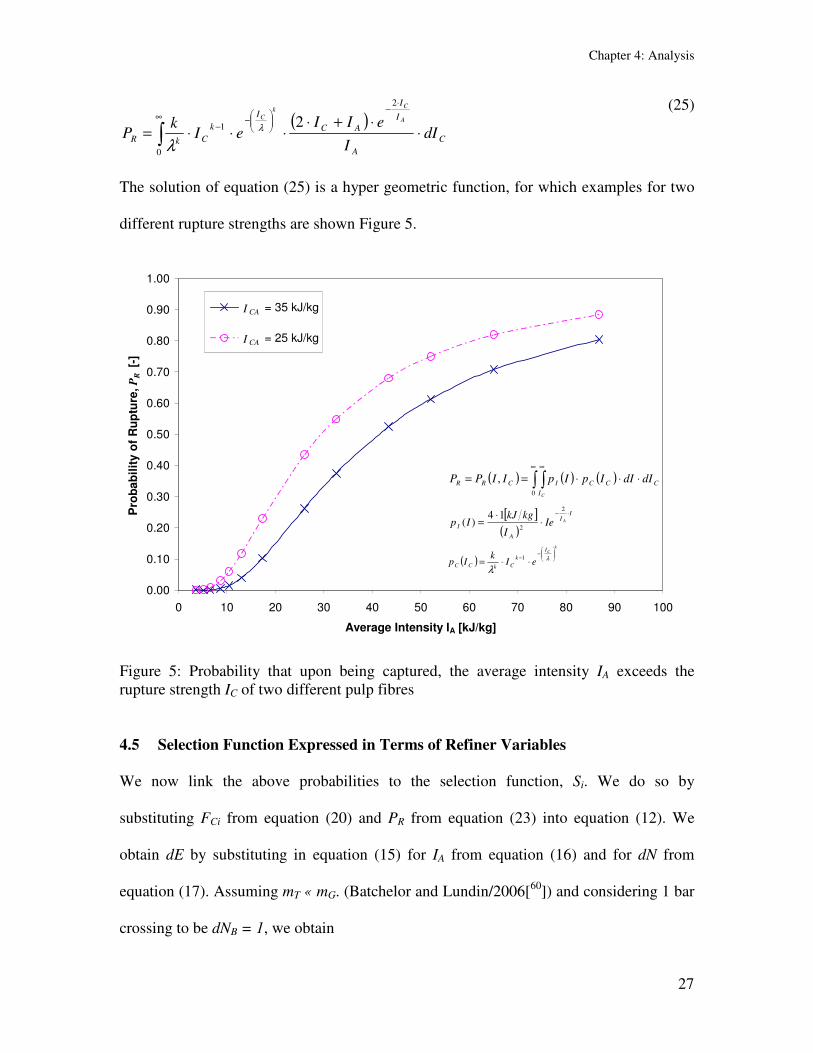
The solution of equation (25) is a hyper geometric function for which examples for two
different rupture strengths are shown Figure 5
000
010
020
030
040
050
060
070
080
090
100
0 10 20 30 40 50 60 70 80 90 100
Average Intensity IA [kJkg]
Pro
bab
ilit
y o
f R
up
ture
P
R [
-]
= 35 kJkg
= 25 kJkg
( ) ( ) ( ) CCC
I
ICRR dIdIIpIpIIPP
C
sdotsdotsdot== int intinfin infin
0
[ ]( )
II
A
IAIe
I
kgkJIp
sdotminus
sdotsdot
=
2
2
14)(
( )
k
CI
k
CkCC eIk
Ip
minus
minussdotsdot= λ
λ
1
I CA
I CA
Figure 5 Probability that upon being captured the average intensity IA exceeds the
rupture strength IC of two different pulp fibres
45 Selection Function Expressed in Terms of Refiner Variables
We now link the above probabilities to the selection function Si We do so by
substituting FCi from equation (20) and PR from equation (23) into equation (12) We
obtain dE by substituting in equation (15) for IA from equation (16) and for dN from
equation (17) Assuming mT laquo mG (Batchelor and Lundin2006[60
]) and considering 1 bar
crossing to be dNB = 1 we obtain
Chapter 4 Analysis
28
( ) ( ) ( ) CCC
I
I
G
ii dIdIIpIpSEL
mlfKS
C
sdotsdotsdotsdotsdotsdot= int intinfin infin
0
(26)
Equation (26) contains three unknowns mT K f(li) These parameters are determined
from Si of the comminution equation However first the relationship between Si and Bij
must be established
46 Relationship between S and B
An analysis relating S and B is shown in Appendix D In brief we first determined a
suitable breakage function to represent probabilities of rupture anywhere along a fibre
length (Olson et al2003[59
]) Previous work by others eg Corte et al1980[80
] assumed
that fibres shortened into only two parts of varying length Our analysis has no such
restriction We determined Bij for a rupture at any point by introducing matrix A that links
Bij and Si giving equation (9) in matrix form as shown below
nAdE
dnsdot= where ( ) SIBA n sdotminus=
(27)
Variable n(E) is a column vector whose entries are the fibre mass fraction in each size
interval after the energy input dE We solved equation (9) by diagonalization of A and
introducing UT as the matrix of the eigenvectors Assuming the process to be Markovian
we re-expressed the population balance as ni(after)=V(E)middotni(before) following the
procedure of Berthiaux2000[84
] We thus decompose V into its characteristic roots
which represent the eigenvalues exp(-SimiddotE) From the matrix of the eigenvectors we
obtained A and from equation (27) the breakage function Bij Further details on this
analysis are given in Appendix D
Chapter 4 Analysis
29
47 Curve -Fitting Procedure
Lastly we selected an appropriate procedure for regression fitting data in fibre length
changes before and after refining to equation (26) to obtain Si We accomplished this in
using GaussndashNewton algorithm method in two steps
First we determined the functional form of the parameter f(li) assuming it to depend on
fibre length alone and to be independent of mT and K This was accomplished by fitting
curve shapes of Si vs fibre length
Next having obtained the form of f(li) we determined parameters mT and K
simultaneously by regression fitting to equation (26) This was accomplished by the same
regression fitting method
Chapter 5 Experimental Program
30
5 Experimental Program
Our experimental program consisted of analyzing fibre length reductions produced by
various refiners We used MatlabTM
software coded to calculate simultaneously the
selection and breakage function for different refining conditions Fibre length
distributions before and after refining were measured using a Fibre Quality Analyzer
(FQATM
) The instrument gives fibre length histograms which contain approximately 150
bins with length increments equal to 005 mm In order to reduce the sampling noise and
the large time associated with calculating a 150 x 150 element transition matrix and
within it the S and B matrix the measured fibre length distributions were compressed into
20 bins with an increment of 025 mm and then normalized Fibres shorter than 05 mm
were included in the measured distributions of this study in contrast to the approach of
Olson et al2003[59
] This may introduce an error because short fibres and fines can be
generated by peeling off pieces of fibre wall rather than by fibre shortening However in
this study all fibres were treated as being a result of fibre shortening The influence of
fines on the overall outcome of the parameter calculation was investigated
The experimental work was carried out in the steps shown as below
Validation of the comminution approach
Evaluation of data from industrial scale pilot plant trials
Evaluation of data from laboratory refiners
Chapter 5 Experimental Program
31
51 Validation of Comminution Approach
The aim of this portion of the experimental work was to validate the comminution
approach by a simple case of comminution examined by Berthiaux2000[84
] described in
Appendix F This was accomplished by employing an easily detectable tracer fibre in
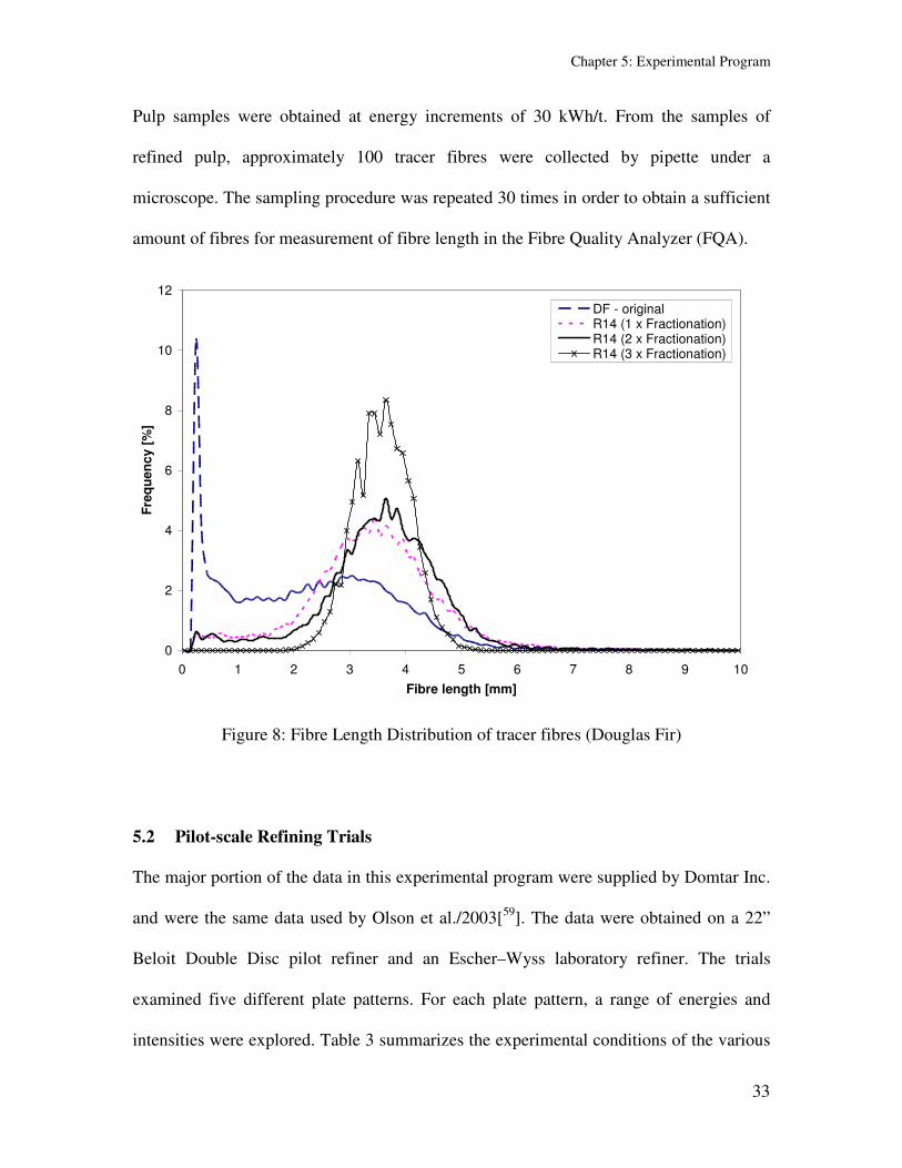
pulp The tracer fibre was a laboratory-produced Douglas Fir pulp cooked using the
ldquokraftrdquo process to an H-factor of 1600 The resultant pulp was carefully washed and later
classified three times in accordance to TAPPI test method T233 cm-95 with the Bauer-
McNett classifier Only the R14 long fibre fraction of the original pulp was retained and
further classified to obtain a narrow distribution (3-4 mm) of long fibres as the tracer As
a result of this procedure we obtained a nearly perfect defect-free pulp having a narrow
length distribution as shown in Figure 8
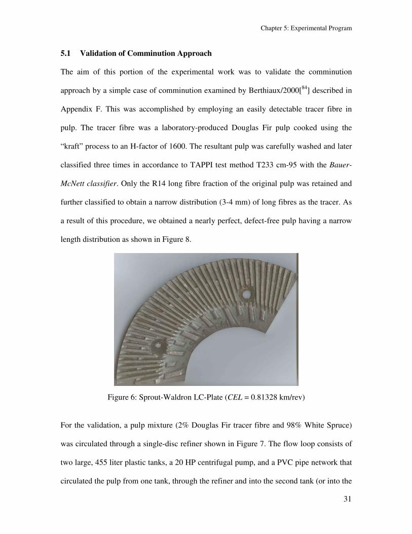
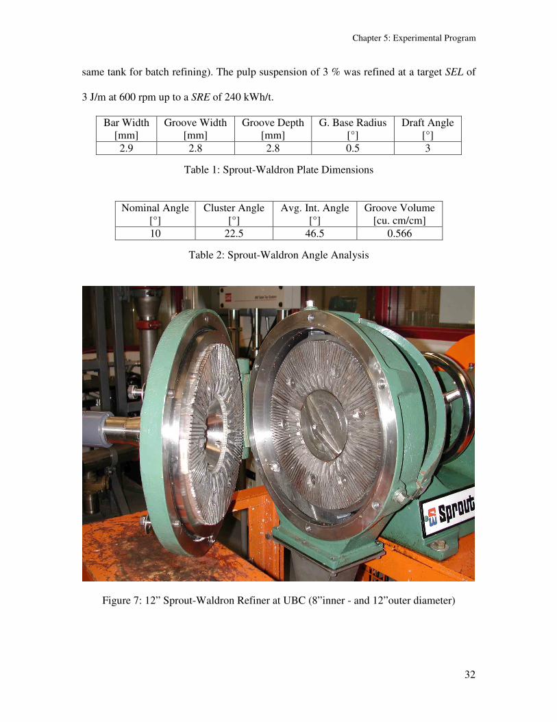
Figure 6 Sprout-Waldron LC-Plate (CEL = 081328 kmrev)
For the validation a pulp mixture (2 Douglas Fir tracer fibre and 98 White Spruce)
was circulated through a single-disc refiner shown in Figure 7 The flow loop consists of
two large 455 liter plastic tanks a 20 HP centrifugal pump and a PVC pipe network that
circulated the pulp from one tank through the refiner and into the second tank (or into the
Chapter 5 Experimental Program
32
same tank for batch refining) The pulp suspension of 3 was refined at a target SEL of
3 Jm at 600 rpm up to a SRE of 240 kWht
Bar Width
[mm]
Groove Width
[mm]
Groove Depth
[mm]
G Base Radius
[deg]
Draft Angle
[deg]
29 28 28 05 3
Table 1 Sprout-Waldron Plate Dimensions
Nominal Angle
[deg]
Cluster Angle
[deg]
Avg Int Angle
[deg]
Groove Volume
[cu cmcm]
10 225 465 0566
Table 2 Sprout-Waldron Angle Analysis
Figure 7 12rdquo Sprout-Waldron Refiner at UBC (8rdquoinner - and 12rdquoouter diameter)
Chapter 5 Experimental Program
33
Pulp samples were obtained at energy increments of 30 kWht From the samples of
refined pulp approximately 100 tracer fibres were collected by pipette under a
microscope The sampling procedure was repeated 30 times in order to obtain a sufficient
amount of fibres for measurement of fibre length in the Fibre Quality Analyzer (FQA)
0
2
4
6
8
10
12
0 1 2 3 4 5 6 7 8 9 10
Fibre length [mm]
Fre
qu
en
cy [
]
DF - originalR14 (1 x Fractionation)R14 (2 x Fractionation)R14 (3 x Fractionation)
Figure 8 Fibre Length Distribution of tracer fibres (Douglas Fir)
52 Pilot-scale Refining Trials
The major portion of the data in this experimental program were supplied by Domtar Inc
and were the same data used by Olson et al2003[59
] The data were obtained on a 22rdquo
Beloit Double Disc pilot refiner and an EscherndashWyss laboratory refiner The trials
examined five different plate patterns For each plate pattern a range of energies and
intensities were explored Table 3 summarizes the experimental conditions of the various
Chapter 5 Experimental Program
34
refiners The reported power is the net power Pnet which is the total power less the no-
load power The consistencies are nominal values The rotational speed for the double
disc refiner (22rdquo Beloit Double Disc) is 900 rpm and for the Escher-Wyss refiner is 1000
rpm The plate dimensions used in this study are summarized in Table 4
Trial Refiner Plate Consistency
[]
mamp
[td]
Pnet
[kW]
SEL
[Jm]
A 284 14 65 325
B 455 14 64 320
C 155 8 34 170
D 248 7 34 170
E
1
422 7 34 170
F 419 9 64 267
G 254 6 26 108
H
2
452 6 26 108
I 270 7 33 014
J 440 7 34 014
K
3
256 4 16 007
L 451 12 55 786
M
22
rdquo B
elo
it D
ou
ble
Dis
c
4 315 13 56 800
N 150 - 07 150
O 300 - 14 300
P 400 - 23 500
Q
Esc
her
-
Wy
ss
5
300 - 23 500
Table 3 Summary of experimental trials from Olson et al[59
]
Plate Bar Width
[mm]
Groove Width
[mm]
Groove Depth
[mm]
Bar angle
[deg]
CEL
[kms]
1 30 30 40 173 2005
2 25 25 50 215 241
3 10 25 10 2125S -265R 2332
4 30 80 40 2125 70
5 60 120 80 160 0521
Table 4 Summary of refiner plate geometries
In addition to measurements of fibre length some key changes in paper properties
resulting from refining were measured namely sheet density burst index tear index
Chapter 5 Experimental Program
35
breaking length tensile index as well as TEA These were measured according to the
appropriate TAPPI standard
53 Escher-Wyss Heterogeneity Trial
Another set of tests was carried on the laboratory Escher-Wyss laboratory refiner in the
Vancouver Laboratory of FPInnovations (Paprican) with assistance of Phil Allen of
FPInnovations This refiner has a rather coarse bar pattern with pulp circulating many
times through the working zone
The following trial plan was employed
Trial
CF
[]
SEL
[Jm]
Energy Increments
[kWht]
1 2 4 306090120
2 3 4 6121824306090120
2 4 4 306090120
4 2 2 306090120
Table 5 Escher-Wyss trial conditions
The Escher-Wyss refiner was set to 1000 rpm The plate patterns used in this study were
the same as for Plate 5 in Table 4
54 Conflo Refining Trial
In addition to the above tests a series of refiner trials were carried out using a industrial-
size Conflo JC-00 conical refiner (angle of conical refiner is 20deg) at various speeds The
tests were carried out with the assistance of Bill Francis and Norman Roberts of
FPInnovations The entry and exit diameters of the rotor of this refiner were 192 mm and
380 mm The refiner plate geometry data are shown in Table 6
Chapter 5 Experimental Program
36
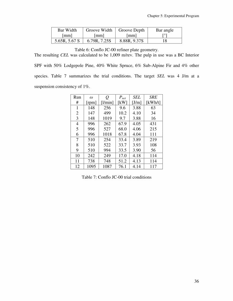
Bar Width
[mm]
Groove Width
[mm]
Groove Depth
[mm]
Bar angle
[deg]
565R 567 S 679R 725S 888R 937S 18
Table 6 Conflo JC-00 refiner plate geometry
The resulting CEL was calculated to be 1009 mrev The pulp in use was a BC Interior
SPF with 50 Lodgepole Pine 40 White Spruce 6 Sub-Alpine Fir and 4 other
species Table 7 summarizes the trial conditions The target SEL was 4 Jm at a
suspension consistency of 1
Run
ω
[rpm]
Q
[lmin]
Pnet
[kW]
SEL
[Jm]
SRE
[kWht]
1 148 256 96 388 63
2 147 499 102 410 34
3 148 1019 97 388 16
4 996 262 679 405 431
5 996 527 680 406 215
6 996 1018 678 404 111
7 510 254 334 389 219
8 510 522 337 393 108
9 510 994 335 390 56
10 242 249 170 418 114
11 738 748 512 413 114
12 1095 1087 761 414 117
Table 7 Conflo JC-00 trial conditions
Chapter 7 Summary and Conclusion
37
6 Results and Discussion
61 Validation of Comminution Approach
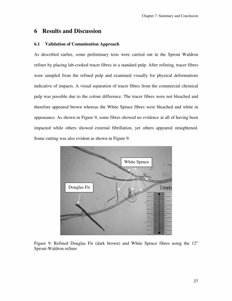
As described earlier some preliminary tests were carried out in the Sprout Waldron
refiner by placing lab-cooked tracer fibres in a standard pulp After refining tracer fibres
were sampled from the refined pulp and examined visually for physical deformations
indicative of impacts A visual separation of tracer fibres from the commercial chemical
pulp was possible due to the colour difference The tracer fibres were not bleached and
therefore appeared brown whereas the White Spruce fibres were bleached and white in
appearance As shown in Figure 9 some fibres showed no evidence at all of having been
impacted while others showed external fibrillation yet others appeared straightened
Some cutting was also evident as shown in Figure 9
Figure 9 Refined Douglas Fir (dark brown) and White Spruce fibres using the 12rdquo
Sprout-Waldron refiner
Douglas Fir
White Spruce
Chapter 7 Summary and Conclusion
38
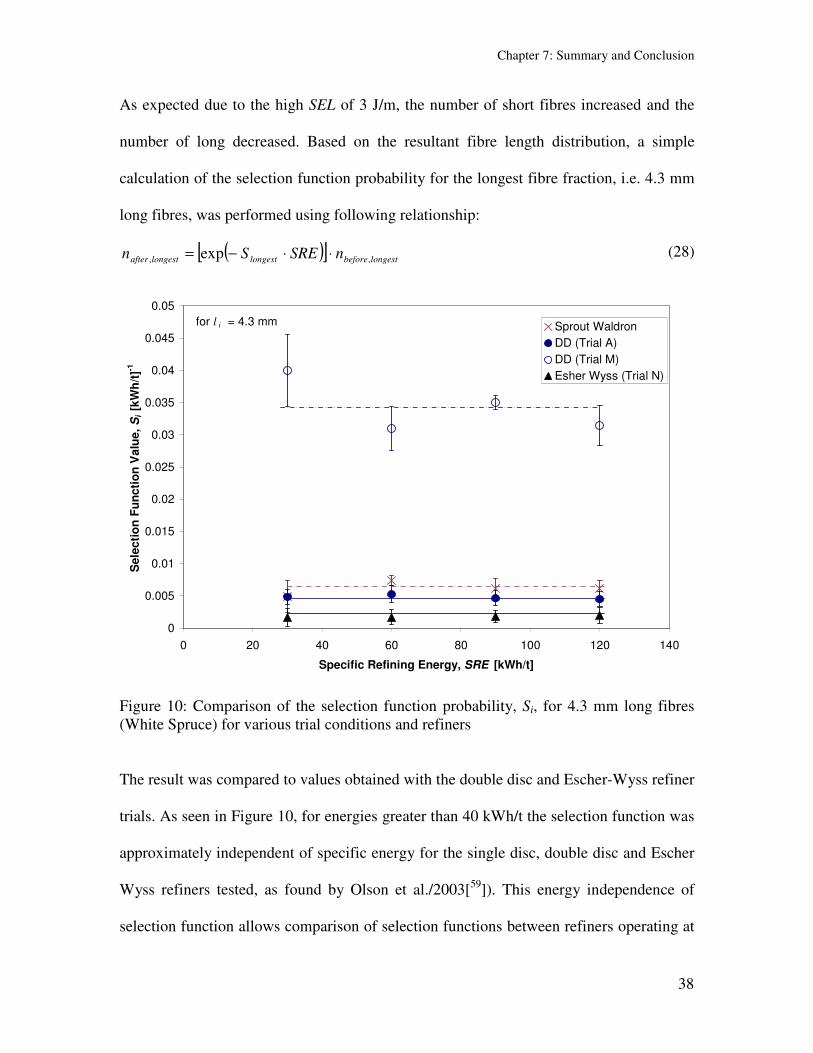
As expected due to the high SEL of 3 Jm the number of short fibres increased and the
number of long decreased Based on the resultant fibre length distribution a simple
calculation of the selection function probability for the longest fibre fraction ie 43 mm
long fibres was performed using following relationship
( )[ ]longestbeforelongestlongestafter nSRESn exp sdotsdotminus= (28)
0
0005
001
0015
002
0025
003
0035
004
0045
005
0 20 40 60 80 100 120 140
Specific Refining Energy SRE [kWht]
Sele
cti
on
Fu
ncti
on
Valu
e
Si [k
Wh
t]-1
Sprout Waldron
DD (Trial A)
DD (Trial M)
Esher Wyss (Trial N)
for l i = 43 mm
Figure 10 Comparison of the selection function probability Si for 43 mm long fibres
(White Spruce) for various trial conditions and refiners
The result was compared to values obtained with the double disc and Escher-Wyss refiner
trials As seen in Figure 10 for energies greater than 40 kWht the selection function was
approximately independent of specific energy for the single disc double disc and Escher
Wyss refiners tested as found by Olson et al2003[59
]) This energy independence of
selection function allows comparison of selection functions between refiners operating at
Chapter 7 Summary and Conclusion
39
different energies It also validates the application of our approach to calculate Si and Bij
using Markov chains However once again the new approach is only possible as long as
there is a measurable amount of cutting
0
0001
0002
0003
0004
0005
0006
0007
0008
0009
001
0 05 1 15 2 25 3 35 4 45
Fibre Length l i [mm]
Sele
cti
on
Fu
ncti
on
Valu
es
Si [
kW
ht
]-1
0
02
04
06
08
1
12
White Spruce
Douglas Fir
Sprout Waldron Refiner
Trial at const SEL = 30 Jm
Obtained by Transition Matrix Approach
Obtained by Tracer Method
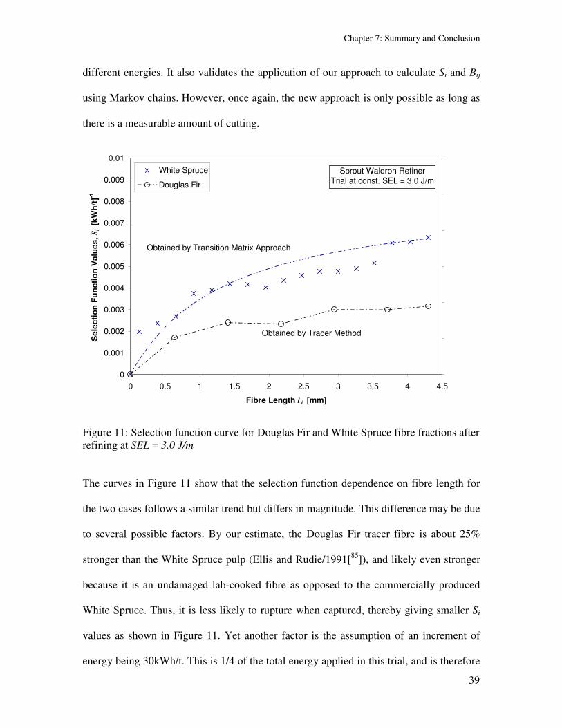
Figure 11 Selection function curve for Douglas Fir and White Spruce fibre fractions after
refining at SEL = 30 Jm
The curves in Figure 11 show that the selection function dependence on fibre length for
the two cases follows a similar trend but differs in magnitude This difference may be due
to several possible factors By our estimate the Douglas Fir tracer fibre is about 25
stronger than the White Spruce pulp (Ellis and Rudie1991[85
]) and likely even stronger
because it is an undamaged lab-cooked fibre as opposed to the commercially produced
White Spruce Thus it is less likely to rupture when captured thereby giving smaller Si
values as shown in Figure 11 Yet another factor is the assumption of an increment of
energy being 30kWht This is 14 of the total energy applied in this trial and is therefore
Chapter 7 Summary and Conclusion
40
very large as an incremental energy In contrast the incremental energy in the matrix-
based estimate is the much smaller energy of an individual bar crossing Nevertheless the
two curves show a similar trend in that fibre shortening increases sharply with increasing
fibre length for small fibres then increases at a smaller rate for longer fibre lengths
62 Selection and Breakage Functions
The statistical significance of the measured differences among the trials were evaluated
by Students t-Test Differences emanating from the transition matrix calculation were
considered statistically significant if the probability associated with a Students t-Test was
smaller than 065 (A value of 0 would mean that the fibres have been cut severely
whereas a value of 1 signifies no cutting meaning a change in arithmetic fibre length less
than 15)
621 Selection Function
We now examine the relationships between selection function and some refining
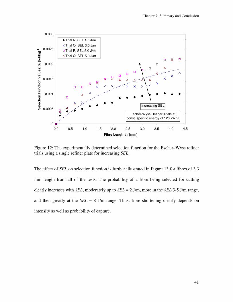
variables at observed length changes Figure 12 shows the selection function dependence
on fibre length for various SELrsquos on the Escher Wyss lab refiner using the same refining
plate The tests were conducted by varying the applied power and pulp consistency It is
apparent that the selection function increases with fibre length but tends to plateau at
longer fibre lengths as found in the tracer fibre studies (Figure 11) For a given fibre
length the selection function increases with increasing SEL meaning increasing power
because the CEL was not changed
Chapter 7 Summary and Conclusion
41
0
00005
0001
00015
0002
00025
0003
00 05 10 15 20 25 30 35 40 45
Fibre Length l i [mm]
Sele
cti
on
Fu
nc
tio
n V
alu
es
Si [
kJk
g]-1
0
01
02
03
04
05
06
07
08Trial N SEL 15 Jm
Trial O SEL 30 Jm
Trial P SEL 50 Jm
Trial Q SEL 50 Jm
Increasing SEL
Escher-Wyss Refiner Trials at
const specific energy of 120 kWht
Figure 12 The experimentally determined selection function for the EscherndashWyss refiner
trials using a single refiner plate for increasing SEL
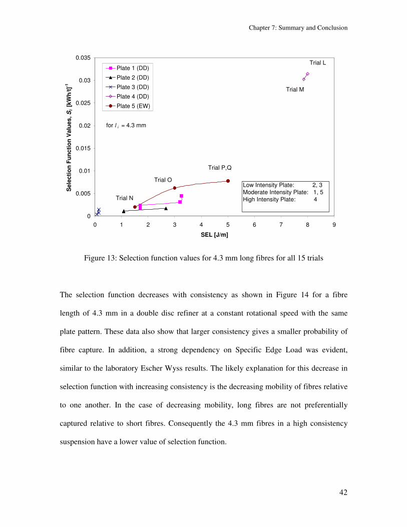
The effect of SEL on selection function is further illustrated in Figure 13 for fibres of 33
mm length from all of the tests The probability of a fibre being selected for cutting
clearly increases with SEL moderately up to SEL = 2 Jm more in the SEL 3-5 Jm range
and then greatly at the SEL = 8 Jm range Thus fibre shortening clearly depends on
intensity as well as probability of capture
Chapter 7 Summary and Conclusion
42
0
0005
001
0015
002
0025
003
0035
0 1 2 3 4 5 6 7 8 9
SEL [Jm]
Sele
cti
on
Fu
ncti
on
Valu
es S
i [
kW
ht
]-1Plate 1 (DD)
Plate 2 (DD)
Plate 3 (DD)
Plate 4 (DD)
Plate 5 (EW)
Trial N
Trial O
Trial PQ
Low Intensity Plate 2 3
Moderate Intensity Plate 1 5
High Intensity Plate 4
Trial M
Trial L
for l i = 43 mm
Figure 13 Selection function values for 43 mm long fibres for all 15 trials
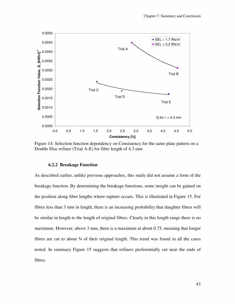
The selection function decreases with consistency as shown in Figure 14 for a fibre
length of 43 mm in a double disc refiner at a constant rotational speed with the same
plate pattern These data also show that larger consistency gives a smaller probability of
fibre capture In addition a strong dependency on Specific Edge Load was evident
similar to the laboratory Escher Wyss results The likely explanation for this decrease in
selection function with increasing consistency is the decreasing mobility of fibres relative
to one another In the case of decreasing mobility long fibres are not preferentially
captured relative to short fibres Consequently the 43 mm fibres in a high consistency
suspension have a lower value of selection function
Chapter 7 Summary and Conclusion
43
00000
00005
00010
00015
00020
00025
00030
00035
00040
00045
00050
00 05 10 15 20 25 30 35 40 45 50
Consistency []
Sele
cti
on
Fu
ncti
on
Valu
e
Si [
kW
ht
]-1SEL = 17 Wsm
SEL = 32 Wsm
Si for l = 43 mm
Trial C
Trial D
Trial E
Trial A
Trial B
Figure 14 Selection function dependency on Consistency for the same plate pattern on a
Double Disc refiner (Trial A-E) for fibre length of 43 mm
622 Breakage Function
As described earlier unlike previous approaches this study did not assume a form of the
breakage function By determining the breakage functions some insight can be gained on
the position along fibre lengths where rupture occurs This is illustrated in Figure 15 For
fibres less than 3 mm in length there is an increasing probability that daughter fibres will
be similar in length to the length of original fibres Clearly in this length range there is no
maximum However above 3 mm there is a maximum at about 075 meaning that longer
fibres are cut to about frac34 of their original length This trend was found in all the cases
tested In summary Figure 15 suggests that refiners preferentially cut near the ends of
fibres
Chapter 7 Summary and Conclusion
44
0
02
04
06
08
1
0 01 02 03 04 05 06 07 08 09 1
Relative Resultant Fibre Length l i l j [-]
Bre
akag
e F
un
cti
on
Bij [
-]43
40
38
35
32
29
27
24
21
19
16
13
10
mm fibre length l j
Figure 15 Breakage probability of White Spruce fibres during trial E
63 Determining Parameters Affecting Selection Function
We now consider the variables which govern the selection function in order to obtain the
key parameters that describe heterogeneity of refining action We do so from equation
(26) which is reproduced below
( ) ( ) ( ) CCC
I
I
G
ii dIdIIpIpSEL
mlfKS
C
sdotsdotsdotsdotsdotsdot= int intinfin infin
0
(26)
There are three unknowns in this equation two K and f(li) describe the probability of
impact and the third unknown mT the mass in the gap gives the average intensity IA
where IA = SEL mT
Chapter 7 Summary and Conclusion
45
631 Determining f(li)
As described earlier the functional form of the length dependence of capture factor f(li)
can be determined from the shapes of curves of the type as shown in Figure 12 (dotted
line) This was accomplished by fitting various length functions to the data by regression
analyses This procedure assumed that K and mT did not affect the form of the function
The form of f(li) examined were once reported by earlier workers eg effect of groove
depth (Kerekes1990[55
]) and consistency (Batchelor and Ludin2006[60
]) The various
forms examined are summarized in Appendix G
The best fit obtained was of the form
( )Dl
llf
i
i
isdot+
=50
(29)
632 Determination of K and mT
The parameters K and mT in equation (26) were determined by regression fitting the data
obtained for Si as function of li to equation (30) below In this equation K is a unknown
constant and mT appears in the average intensity IA (IA = SEL mT) in the integrals
( ) ( ) CCC
I
I
G
i
i
i dIdIIpIpSEL
m
Dl
lKS
C
sdotsdotsdotsdotsdotsdot+
sdot= int intinfin infin
050
(30)
The results from the regressions are shown in Table 8 A representative energy input of
SRE = 120 kWht was arbitrary chosen for the regression The average number of
impacts NA experienced by fibres was calculated from NA = mT mG NB (equation (17))
Chapter 7 Summary and Conclusion
46
Trial Plate Refiner Plate Intensity SRE SEL m G C F K m T m T m G I A N A
(SEL ) [kJkg] [kJm] [kgm] [] [-] [kgm] [-] [kJkg] [-]
A 4500 000324 682E-04 284 0062 166E-04 0244 195 23
B 4320 000319 109E-03 455 0051 206E-04 0189 155 28
C 4140 000170 372E-04 155 0040 963E-05 0259 177 23
D 4356 000171 595E-04 248 0015 849E-05 0143 201 22
E 4392 000171 101E-03 422 0012 100E-04 0099 170 26
F 4140 000267 105E-03 419 0023 176E-04 0168 152 27
G 4140 000108 635E-04 254 0007 623E-05 0098 173 24
H 4212 000108 113E-03 452 0005 658E-05 0058 164 26
I 3276 000014 135E-04 270 0069 360E-05 0267 39 84
J 4464 000014 220E-04 440 0011 637E-05 0289 22 203
K 4248 000007 128E-04 256 0004 282E-05 0220 25 171
L 4320 000786 289E-03 451 0068 198E-04 0069 396 11
M 4140 000800 202E-03 315 0115 231E-04 0114 347 12
N 4324 000150 288E-03 150 0003 662E-05 0023 227 19
O 4291 000300 576E-03 300 0022 123E-04 0021 243 18
P 4280 000500 768E-03 400 0008 166E-04 0022 301 14
Q 4270 000500 960E-03 300 0007 205E-04 0021 244 18
4 4 highest
5 EW 5 moderate
1
DD
1 moderate
2 2 low
3 3 ultra-low
Table 8 Comparison of obtained values for K mT IA and NA for a representative specific
energy input of 120 kWht (all are converted into SI-units)
64 Discussion of Predicted Probabilities and Intensities
We now examine and compare the probabilities of impacts (capture) and the average
intensity of impacts on fibres obtained from the regression analysis
641 Probability of Impact
Recalling from equation (29) that the factor of capture of a fibre of length li at a single bar
crossing is given by FCi = K (li + 05D) we now examine factors which affect this
probability As expected FCi increases with decreasing groove depth as shown in Figure
16 This occurs because the fibre capture sweep zone by a bar edge occupies a larger
fraction of the total groove depth It is further evident in Figure 16 that FCi increases with
increasing groove width up to about 5 mm and then decreases beyond this level The
likely explanation for increasing FCi is that a wider groove gives a longer sweep zone
which enables more fibre capture However this increase has a limit which is likely the
capacity of the gap to hold fibre or the maximum mass of fibres which a bar edge can
Chapter 7 Summary and Conclusion
47
capture Such a limit was observed by Smith1922[24
] in drawing a bar through an infinite
reservoir of pulp For example he found that at 3 consistency pulp a bar captured
fibres up to a level of about 0001 kgm We may note here that a sweep length of 5 mm
over a depth equal to a fibre length of 25 mm contains about 00004 kgm pulp For a
sweep length of 12 mm this would be about 0001 kgm which is about the limit found
by Smith1922[24
]
The probability of fibre impact also depends on flow conditions in a refiner This is
shown in Figure 17 As radial flow velocity increases the probability of fibre impact
increases for an average constant tangential velocity of 263 ms (in case of the double
disc refiner) or 61 ms (Escher Wyss laboratory refiner) respectively
000
001
002
003
004
005
006
007
008
0 2 4 6 8 10 12 14
Groove Width G [mm]
K
l A
( lA
+0
5
D)
[-]
Plate 1 (DD)
Plate 2 (DD)
Plate 3 (DD)
Plate 4 (DD)
Plate 5 (EW)
D = 40 mm
D = 50 mm
D = 10 mm
D = 40 mm
D = 80 mm
for l A = 220 mm
Figure 16 Probability of capture for average fibre length lA during one bar crossing for
various plate geometries
Chapter 7 Summary and Conclusion
48
000
001
002
003
004
005
006
007
008
000 001 002 003 004 005 006 007
Average Radial Velocity vradial [ms]
K
l A
( lA
+0
5
D)
[-]
Plate 1 (DD)
Plate 2 (DD)
Plate 3 (DD)
Plate 4 (DD)
Plate 5 (EW)
G = 25 mm
G = 30 mm
G = 80 mm
G = 120 mm
for l A = 220 mm
Figure 17 Capture probability for average fibre length lA during one bar crossing for
various flow conditions
642 Intensity of Impacts
Values for the average intensity of impact IA are shown in Table 8 For a given SEL IA
depends on mT The values of mT from the regression vary from 23middot10-4
kgm to 283middot10-5
kgm a range which appears reasonable For example assuming a consistency for the
compressed fibre mat in a refiner gap to be of 30 a gap of size 015mm and 3 mm bar
width would hold about 10-4
kgm of fibres
The values of mT obtained give levels of IA in Table 8 from 22kJkg to 396 kJkg This
range is also reasonable Evidence of this is shown by fibre shortening in Figure 18
where fibre length is relatively unaffected up to an average intensity of about 20 kJkg
then diminishes significantly as intensity increases beyond this value
Chapter 7 Summary and Conclusion
49
R2 = 09477
0
05
1
15
2
25
0 5 10 15 20 25 30 35 40 45 50
Average Intensity I A [kJkg]
Ave
rag
e F
ibre
Le
ng
th l
LW
[m
m]
Unrefined
Plate 1 (DD)
Plate 2 (DD)
Plate 3 (DD)
Plate 4 (DD)
Plate 5 (EW) SRE = 120 kWht
Figure 18 Fibre-length-reduction characterization as function of intensity
0
001
002
003
004
005
006
007
008
0 5 10 15 20 25 30 35 40 45 50
Intensity I [kJkg]
Pro
ab
ab
ilit
y D
istr
ibu
tio
n p
I(I)
[-]
Trial D
Rupture Strength Fibres
I A = 20 kJkg
I CA = 35 kJkg
Figure 19 Actual intensity distribution vs the distribution of rupture strength IC
Chapter 7 Summary and Conclusion
50
The estimated fibre rupture strength is 35 kJkg meaning that values in the high end of
the distribution about 20 kJkg exceed this value This takes place as shown in
Figure 19
65 Comparisons to Previous Studies
651 Intensities
We now compare findings of this study to other relevant published work Leider and
Nissan1977[36
] and Kerekes1990[55
] predicted intensities by dividing the specific
energy by the estimated number of impacts on pulp fibres Their predicted intensities are
compared to values from this study in Figure 20
0
5
10
15
20
25
30
35
40
45
0 5 10 15 20 25 30 35 40 45
Estimated Intensity by other Authors I [kJimpkg]
Avera
ge I
nte
nsit
y f
rom
th
is S
tud
y I
A [
kJk
g]
C-Factor Analysis (Kerekes)
Leider and Nissan Theory
DD refiner (Trial A-M)
Figure 20 Comparisons of Average Intensity IA to intensity levels calculated based on
previous studies by Leider and Nissan1977[36
] and Kerekes1990[55
]
Chapter 7 Summary and Conclusion
51
Clearly the C-Factor predicts larger values then those of this study whereas Leider and
Nissan1977[36
] predict smaller values Thus the results of this study fall between the
values of these earlier studies Leider and Nissan predict low intensities because they
estimate many more impacts than does the C-Factor They assumed that the number of
impacts per fibre per bar crossing is proportional to the ratio of cross-sectional area of a
fibre to the cross-sectional area of a groove as well as to the rotational speed On the
other hand Kerekesrsquo C-Factor assumed the probability of impact to depend upon the ratio
lA (lA + D) and suspension consistency justifying these assumptions by showing that
they led to logical outcomes in limiting cases
652 Probabilities of Impacts in Compression Refining
In recent work Goosen et al2007[86
] showed that for compression refining the
development of tensile strength in paper was strongly linked to the probability that fibres
experience one impact (loading cycle) This observation suggested that the role of
multiple loading cycles in refining was to ensure that many fibres experienced at least
one impact as opposed to the conventional view that the purpose of multiple loading
cycles was to introduce fatigue weakening By a simple statistical model Goosen et
al2007[86
] showed that increase in tensile strength R(NC) was related to the cumulative
probability of an impact P over NC cycles
( ) ( ) CN
C PNR minusminus= 11 (31)
We tested this relationship on the EW refiner by obtaining the tensile strength for given
numbers of bar crossings NB (in place of NC) as shown in Table 9 and plotted in Figure
21 By regression fitting to equation (31) to these data we obtained the probability P that
gave the best fit
Chapter 7 Summary and Conclusion
52
CF SEL SRE [kWht]
[] [Jm] 6 12 18 24 30 60 90 120
NB [-] 207 415 622 829 2 2
BL [km] 4553 6105 7152 7604
NB [-] 104 207 311 415 2 4
BL [km] 4878 5918 7058 7672
NB [-] 31 62 93 124 156 311 467 622 3 4
BL [km] 3396 3869 4154 4376 4646 565 6138 7151
NB [-] 207 415 622 829 4 4
BL [km] 4454 5805 6697 6814
Table 9 Escher-Wyss trails including calculated number of bar crossings NB and
breaking length BL
27
37
47
57
67
77
87
0 100 200 300 400 500 600 700 800 900
Number of bar crossings N B [-]
Bre
akin
g L
en
gth
[km
]
00
01
02
03
04
05
06
07
08
09
10
R(N
B) [
-]
C=2 SEL=2Jm
Commulative probability of fibre being refined
00210=P
( ) ( ) BNB PNR minusminus= 11
Figure 21 Tensile strength plotted against cumulative probability for P = 00021
The result for a consistency of 2 and an SEL = 2 Jm was P = 00021 This value
is close to the value of FCi = 00023 obtained from KmiddotlA (lA+05middotD) in Table 8 for the
Escher Wyss trials of the previous section For all four combinations of consistency and
SEL probability P ranged from 00019 to 00045 Though not conclusive this finding
seems to confirm that probabilities of impacts found in this study are sound as can be
Chapter 7 Summary and Conclusion
53
seen in Figure 22 It further suggests that the role of multiple loading cycles in refining is
to ensure that many fibres see at least one impact as opposed to introducing fatigue
weakening in short that the role of multiple loading cycles is to reduce heterogeneity
0
001
002
003
004
005
006
007
0 001 002 003 004 005 006 007
Kl A (l A +05D) [-]
P [
-]
Trial A - Q
Figure 22 Comparison of KlA (lA+05D) and P for Trials A - Q
66 Homogeneity Index
We now address the question of defining a useful parameter to represent heterogeneity
For convenience in order to have a larger value represent a better result we will define
heterogeneity in terms of its inverse ndash homogeneity A ldquoHomogeneity Indexrdquo may be
used to characterize operating refiners From an industrial standpoint it is desirable to
have a single number index However in reality this is difficult Homogeneity is affected
by the number and intensity of impacts as well as by the distribution of each of these
variables Moreover each of these has subset of additional factors All this gives rise to
Chapter 7 Summary and Conclusion
54
many possible combinations of parameters that could be employed to define a
homogeneity index H Somewhat arbitrarily we choose the following the product of the
number of impacts on fibres of average length and the fraction of intensities within +- 2
kJkg of the average intensity divided by the specific refining energy SRE This can be
expressed as
( )
SRE
IkgkJIPNDl
lK
H
AAB
A
A sdotplusmnsdotsdotsdot+
sdot
=
250
(32)
Values of H for our tests are summarized in Table 10 along with the key refiner variables
and computed parameters
Trial Plate Refiner Plate Intensity SRE SEL m G C F m T N B I A N A H
(SEL ) [kJkg] [kJm] [kgm] [] [kgm] [-] [kJkg] [-] [-]
A 4500 000324 682E-04 284 166E-04 95 195 23 0015
B 4320 000319 109E-03 455 206E-04 148 155 28 0020
C 4140 000170 372E-04 155 963E-05 91 177 23 0010
D 4356 000171 595E-04 248 849E-05 152 201 22 0006
E 4392 000171 101E-03 422 100E-04 260 170 26 0008
F 4140 000267 105E-03 419 176E-04 162 152 27 0009
G 4140 000108 635E-04 254 623E-05 243 173 24 0004
H 4212 000108 113E-03 452 658E-05 441 164 26 0005
I 3276 000014 135E-04 270 360E-05 316 39 84 0116
J 4464 000014 220E-04 440 637E-05 701 22 203 0027
K 4248 000007 128E-04 256 282E-05 777 25 171 0011
L 4320 000786 289E-03 451 198E-04 159 396 11 0028
M 4140 000800 202E-03 315 231E-04 104 347 12 0033
N 4324 000150 288E-03 150 662E-05 830 227 19 0005
O 4291 000300 576E-03 300 123E-04 824 243 18 0012
P 4280 000500 768E-03 400 166E-04 657 301 14 0009
Q 4270 000500 960E-03 300 205E-04 820 244 18 0008
EW 5 moderate
1
2
3
4
5
DD
1
4 highest
moderate
2 low
3 ultra-low
Table 10 Summary of Pilot-scale Refining Trials results
Several observations can be made from Table 10 The value of H for the Escher-Wyss
refiner is similar to that for the Double Disc refiners when comparisons are made at a
similar consistency rotational speed and SEL This is unexpected for the very coarse bar
patterns of the EW However in this refiner pulp circulates through it many times
whereas pulp passes only once through the Double Disc refiners Thus extended
Chapter 7 Summary and Conclusion
55
residence time can compensate for coarse bar pattern Another unexpected result is the
large values of H for the ldquoultra-low intensityrdquo (Trials I ndash K) over an SEL range from 007
to 014 Jm The low intensity in these trials was compensated for by a large number of
impacts to give the same SRE more than four times the number in other cases studied to
give the same refining energy This suggests that number of impacts is a much stronger
factor than intensity in determining homogeneity of treatment
0000
0002
0004
0006
0008
0010
0012
0014
0016
0018
0020
0 200 400 600 800 1000 1200
Flow Q [lmin]
Ho
mo
gen
eit
y I
nd
ex H
[-]
130
250
500
1000 rpm
1000 rpm
510 rpm
510 rpm
1000 rpm
1100 rpm
750 rpm
250 rpm
CONFLOW JC-00
SEL=4 Wsm
C = 1
Number of bar crossings N B
Figure 23 Homogeneity development in dependency of throughput and refiner speed
using a CONFLO refiner at 1 consistency and SEL = 4 Jm
Flow conditions in refiners also affect H This factor was evaluated in the CONFLO
refiner by varying the rotational speed and throughputs while keeping the SEL constant
The findings are shown in Figure 23 It shows that for a given number of bar crossings
higher throughput flow rate increases refining homogeneity This agrees with Figure 17
which showed that increasing radial velocity through a refiner increased the probability
Chapter 7 Summary and Conclusion
56
of fibre impact at a bar crossing The higher H may be due to more effective fibre mixing
due to larger shear and turbulence
6
8
10
12
14
16
18
20
0 001 002 003 004 005 006 007 008 009 01
Homogeneity Index H [-]
Tear
Ind
ex [
mNm
2g
]
Plate 1 (DD) - SEL = 1732 Jm
Plate 2 (DD) - SEL = 1027 Jm
Plate 3 (DD)- SEL = 007014 Jm
Plate 4 (DD)- SEL = 7880 Jm
Plate 5 (EW)- SEL = 1550 Jm
Figure 24 Relationship between Tear Index and Homogeneity Index H
Relationship between tear index and homogeneity is shown Figure 24 The ultra-low
intensity plate (3) had the smallest loss in tear (shown as the largest tear strength) The
other plates all caused a significant reduction in tear strength to the 10 ndash 12 mNm2g
range with the largest intensity (SEL) accomplishing this with the greatest homogeneity
In summary the experimental results described above show that the analysis depicted in
Section 4 presents a useful basis for characterizing uniformity of treatment of pulp fibres
in refiner Moreover the results show that previous estimates of intensities of impact are
either too large or too small and that the probability of impact corresponds with previous
measurements of probability of successful loading cycle in compression refining
Chapter 7 Summary and Conclusion
57
7 Summary and Conclusions
A method to measure heterogeneity of treatment in pulp refiners has been developed
using comminution theory and measurements of fibre length before and after refining
This was accomplished by interpreting the selection and breakage functions of the
comminution equation in terms of a single bar crossing event namely probability of
impact with fibres intensity distribution of impact and location of breakage along a fibre
length These probabilities were interpreted in terms of heterogeneity of treatment
The method was applied to measure heterogeneity of treatment in three different types of
refiners a pilot disc refiner an industrial disc refiner and an Escher-Wyss laboratory
refiner This was accomplished by regression fitting the comminution equation to
measured fibre length distributions before and after refining under various operating
conditions The measured probabilities and intensities of impact showed some key
findings
- probability of fibre impact at a bar crossing event increases with decreasing
groove depth and increasing groove width up to about a groove width of 10 mm
then decreases
- probability of fibre impact at a bar crossing event increases with radial pulp flow
velocity
- intensity levels were larger than those predicted by Leider and Nissan1977[36
]
and smaller than those predicted by Kerekes1990[55
]
- increase in tensile strength of pulp with refining was consistent with the
cumulative probability of experiencing a loading cycle during a bar crossing
Chapter 7 Summary and Conclusion
58
event in agreement with the findings of Goosen et al2007[86
] for loading cycles
in compression refining
The results of this work enable refining heterogeneity to be characterized in a number of
different ways A simple one chosen somewhat arbitrarily is a ldquoHomogeneity Indexrdquo
defined as the number of impacts on fibres having the average fibre length multiplied by
the fraction of intensities within +- 2 kJkg of the average intensity divided by the
specific refining energy This index provided quantitative measurement of factors
affecting homogeneity postulated qualitatively by earlier workers such as
- increased flow rate through the refiner increased homogeneity of treatment
- large numbers of impacts at low intensities give greater homogeneity at a given
specific energy than do smaller numbers of impacts at higher intensities
- large residence time in refiners can offset heterogeneity caused by very coarse bar
pattern
Chapter 8 Recommendations
59
8 Recommendations
This thesis has established a foundation upon which future work can build This work
could take several forms for example further development of the method or applying it to
refiners to correlate results with changes in pulp properties
For further development of the approach perhaps the greatest need is a measurement of
the amount of pulp captured in a refiner gap the variable called mT in this thesis
Predicted values of intensity from this work seem reasonable falling between values
predicted by other workers However a definitive measurement linked to refiner
variables which affect mT would be of great value
Another further development could be the use of force rather than energy as the basis of
intensity related to strain and rupture of fibres To obtain such forces detailed knowledge
of fibre distribution in refiner gaps as well as the amount of fibres is needed
On the question of applying this method a comprehensive set of experiments ought to be
carried out in which key pulp properties are linked to homogeneity of treatment defined
in several ways
In applying the method to mill refiners it is recognized that most refiners are operated to
minimize fibre cutting Consequently the concept of a ldquobump testrdquo should be explored in
which power is increased for a short period to deliberately cut fibres for this test While
the conditions of a bump test differ from the operating condition the difference can be
Chapter 8 Recommendations
60
taken into account in the analysis to obtain a useful characterization of homogeneity of
treatment obtained
Lastly there are other potential ldquohomogeneity indicesrdquo than the one presented here
These should be explored Perhaps the benefits of a two-parameter index outweigh the
simplicity of a one-parameter index and this too should be explored
References
61
References
[1] Higgins H G and Jde Yong The beating process Primary effects and their
influence on pulp and paper properties In The formation and structure of paper
Transactions of the symposium held at Oxford September 1961 ed F Bolam
London Technical Section British Paper and Board Makers Association 2 651ndash
97 (1962)
[2] Page DH The mechanism of strength development of dried pulps by beating
Svensk Papperstidning 88(3) R30-R35 (1985)
[3] Seth RS Optimizing reinforcement pulps by fracture toughness TAPPI Journal
79(1) 170-178 (1996)
[4] Hiltunen E Kettunen H Laine J E Paulapuro H Behaviour of reinforcement
fibres in TMP-based paper Paperi ja Puu ndash Paper and Timber vol 84 no 4 pp
269-273 (2002)
[5] Atack D Towards a theory of refiner mechanical pulping Appita Journal 34(3)
223-227 (1980)
[6] Page D The Beating of Chemical Pulps--The Action and Effects Trans of
Fundamental Symposium (F Bolam Ed) Tech Sect BPampBMA Oxford (1989)
[7] Danforth DW The effect of refining parameter on paper properties Advances in
refining technology PIRA England (1986)
[8] Page DH Ksky J Booth D Some initial observations on the action of the
beater What are we doing BP + BMA Bull 28 1 ndash 7 (1962)
[9] Atack D Advances in beating and refining Trans Fund Res Symp Oxford
Pulp and Paper Fundamental Research Society UK pp261ndash 269 (1977)
References
62
[10] Ebeling K A Critical Review of Current Theories for the Refining of Chemical
Pulps International Symp On Fund Concepts of Refining IPST Appleton USA
pages 1-33 (1980)
[11] Hietanen S ndash Development of a fundamentally new refining method Paperi ja Puu
72(9)874 (1990)
[12] Hietanen S Ebeling K A new hypothesis for the mechanics of refining Paperi ja
Puu 72(2)37-44 (1990)
[13] Mohlin U-B Miller J Industrial refining - effects of refining conditions on fibre
properties 3rd International refining Conference and Exhibition March 20-22
Atlanta USA PIRA paper 4 (1995)
[14] Seth RS The importance of fibre straightness for pulp strength Pulp amp Paper
Canada 107(1) T1-T9 (2006)
[15] Mohlin U-B Cellulose fibre bonding Part 3 The effect of beating and drying on
interfibre bonding Svensk Papperstidning 78(9) 338-341 (1975)
[16] Kerekes RJ Tam Doo PA Wet fibre flexibility of some major softwood species
pulped by various processes 71st Annual Meeting CPPA Montreal Canada
January 29-30 Preprints A 45-46 (1985)
[17] Paavilainen L Conformability - flexibility and collapsibility - of softwood
sulphate pulp fibres Paperi ja Puu 75(9-10) 689-702 (1993)
[18] Page DH De Grace JH Delamination of fiber walls by beating and refining
TAPPI Journal Vol 50(10) 489-495 (1967)
[19] Clark JD Fibrillation free water and fiber bonding TAPPI Journal Vol
52(2)335-340 (1969)
References
63
[20] Hartman RR Mechanical treatment of pulp fibers for paper property
development Transactions of the Eighth Fundamental Research Symposium held at
Oxford England September 1985 Mechanical Engineering Publications Limited
London Vol 1 413-442 (1985)
[21] Kerekes RJ Perspectives on Fiber Flocculation in Papermaking Proceedings
International Paper Physics Conference Niagara-on-the-lake ON Canada pp23-
31 (1995)
[22] Mohlin U-B Low consistency beating - laboratory evaluation contra industrial
experience Current and future technologies of refining Conference Proceedings
10-12 December 1991 PIRA Leatherhead UK Volume 1 Paper 01 14 pages
(1991)
[23] Seth RS Zero-span tensile strength of papermaking fibres Paperi ja Puu 83(8)
597-604 (2001)
[24] Smith SF The action of the beater in papermaking Paper Trade Journal
106(26)47 (1922)
[25] Rance H F In Symposium on Beating Proceedings Technical Section British
Paper and Board Makers Association 32(2)360-70 (1951)
[26] Steenberg B In Symposium on Beating Proceedings Technical Section British
Paper and Board Makers Association 32(2)388-95 (1951)
[27] Frazier WC Applying hydrodynamic lubrication theory to predict refiner
behavior Journal of Pulp and Paper Science Vol14 No 1 J1-J5 (1988)
[28] Roux JC Hydrodynamic modelling of the behaviour of the pulp suspensions
during beating and its application to optimising the refining process 11th
Fundamental Research Symposium Cambridge UK 21-26 September (1997)
References
64
[29] Lundin T Loumlnnberg B Harju K Soini P LC - Beating of Pulp Fibres Pulping
Conference Proceedings (1999)
[30] Halme M Syrjanen A Flow of stock in a conical refiner as observed by high
speed film camera Atti Cong Eur Tech Carteuria Venice PIRA pp 273ndash 277
(1964)
[31] Herbert W and Marsh PG Mechanics and Fluid Dynamics of a Disk Refiner
TAPPI Journal Vol 51 No 5 pp 235-239 (1968)
[32] Banks WA Design considerations and engineering characteristics of disc refiners
Paper Technology 8 (4) 363ndash 369 (1967)
[33] Goncharov VN Force factors in a disc refiner and their effect on the beating
process Bum Prom 5 12ndash14 (1971)
[34] Fox TS Brodkey RS Nissan AH High speed photography of stock transport
in a disc refiner TAPPI Journal Vol 62 (3) 55ndash 58 (1979)
[35] Leider PJ Rihs J Understanding the disk refiner TAPPI Journal Vol60 no9
pp98-102 (1977)
[36] Leider PJ Nissan AH Understanding the disc refinermdashthe mechanical
treatment of fibres TAPPI Journal Vol 60 (10) 85ndash 89 (1977)
[37] Fox T S Pulp transport in the disk refiner Paper presented at the 50th
anniversary of The Institute of Paper Chemistry Appleton WI p49 (1979)
[38] Arjas A Jankola 0 and Ryti N Paperi ja Puu 51(12)869-79 (1969)
[39] Batchelor WJ and Lundin T - A method to estimate fibre trapping in low
consistency refining TAPPI Journal Vol 5(8)31 (2006)
References
65
[40] Kerekes RJ Olson JA Perspectives on fibre length reduction in refining In
proceedings of 7th PIRA international refining conference amp exhibition In
proceedings of 7th PIRA international refining conference amp exhibition 25-26
March Stockholm Sweden March 25-26 paper 5 (2003)
[41] Steenberg B ndash Mahlungsvorgaenge ndash Neue Betrachtungen ndash Das Papier
Darmstadt 35 10A S V141-V149 (1979)
[42] Goosen D Olson JA Kerekes RJ The Role of Heterogeneity in Compression
Refining Journal of Pulp and Paper Science 33(2)110-114 (2007)
[43] Goncharov VN Force Factors in a Disk Refiner and Their Effect on the Beating
Process Bum Promst 12(5) 1-14 (1971)
[44] Martinez DM Batchelor WJ Kerekes RJ and Ouellet D - Forces on fibres
in refining - normal force Journal of Pulp and Paper Science 23(1)J 11 (1997)
[45] Batchelor WJ Martinez DM Kerekes RJ and Ouellet D - Forces on fibres
in refining - shear force Journal of Pulp and Paper Science 23(1)J 40 (1997)
[46] Kerekes RJ Senger JJ Characterizing Refining Action in Low-Consistency
Refiners by Forces on Fibres Journal of Pulp and Paper Science 32(1)1-8 (2006)
[47] Koskenhely K Nieminen K Paulapuro H Edge form profile of refiner filling
bars and its impact on softwood fibre shortening Paperi ja Puu vol 89 no4 pp
236-241 (2007)
[48] Wultsch F Flucher W Der Escher- Wyss-Kleinrefiner als Standard Pruumlfgeraumlt
fuumlr moderne Stoffaufbereitungsanlagen Das Papier 12(13)334-342 (1958)
[49] Brecht W SiewertWH Zur theoretisch-technischen Beurteilung des Mahl-
prozesses modern Mahlmaschinen Das Papier 20(10)4-14 (1966)
References
66
[50] Lumiainen J A new approach to the critical factors effecting on refining intensity
and refining results in low consistency refining TAPPI Papermakers Conference
Proceedings TAPPI Press Atlanta (1990)
[51] Meltzer FP Rautenbach R Neue Moeglichkeiten zur Vorherbestimmung des
technologischen Mahlergebnisses Das Papier 48 (9) 578ndash 583(1994)
[52] Lewis J and Danforth D W Stock preparation analysis TAPPI Journal
45(3)185-88 (1962)
[53] Danford DW Southern Pulp and Paper Manufacturer pp 52 (1969)
[54] Van Stiphout J M J A preliminary study of refining action on cellulose fibers
TAPPI Journal 47(2)189A-91A (1964)
[55] Kerekes RJ Characterization of pulp refiners by a C-factor Nordic Pulp and
Paper Journal 5(1) p2-8 (1990)
[56] Steenberg B Svensk Papperstidning 66(22)933-939 (1963)
[57] Halme M Paperi ja Puu 44(12)658-60 (1962)
[58] Ryti N and Arjas A Paperi ja Puu 51 (1) 69 (1969)
[59] Olson JA Drozdiak J Martinez M Garner R Robertson A Kerekes RJ
Characterizing fibre shortening in a low-consistency refining using a comminution
model Powder Technology 129 pp 122ndash129 (2003)
[60] Batchelor WJ and Lundin T - A method to estimate fibre trapping in low
consistency refining TAPPI Journal 5(8)31 (2006)
[61] Batchelor W and Ouellet D - Estimating forces on fibres in refining Proceedings
4th International Refining Conference PIRA International Leatherhead UK p
Paper 2 (1997)
References
67
[62] Roux JC Joris G Angular parameters beyond specific edge load TAPPSA
Journal No 7 (2005)
[63] Endres I Vomhoff H Stroumlm G New Sensor Technique for Measuring Small-
Scale Pressure Distributions International Paper Physics Conference Victoria BC
(2003)
[64] Prairie B Wild P Byrnes P Olender D Francis DW and Ouellet D Forces
During Bar-Passing Events in Low Consistency Refining Effects of Refiner Tram
Pulp amp Paper Canada 109(9)T153-T156 (2007)
[65] Page DH The origin of the differences between sulphite and kraft pulps Journal
of Pulp and Paper Science March TR 15-TR20 (1983)
[66] Hietanen S The Role of Fiber Flocculation in Chemical Pulp Refining Paperi ja
Puu - Paper and Timber 73(3) 249-259 (1991)
[67] Lumiainen J ndash Comparison of mode of operation of conical and disc refiners PTS-
IZP 1CALAR-Symposium 01121995 Heidenau GER (1995)
[68] Simons F L TAPPI Journal 33(7)312-4 (1950)
[69] Nisser H amp Brecht W lsquoZwei neue Messkriterien von aufgeschwemmten Fasern
zur Beurteilung der Blattfestigkeitrsquo Svensk Papperstidning 66(2) pp 37ndash41
(1963)
[70] Mohlin U-B and O Lidbrandt Changes in fiber structure due to refining as
revealed by SEM Pages 61-74 in International symposium on fundamental
concepts of refining Appleton WI (1980)
[71] Dharni S Kerekes RJ Estimation of the number of impacts imparted to the pulp
in a disc refiner Master of Pulp and Paper Eng Project Report UBC Pulp and
Paper Centre (1989)
References
68
[72] Dekker JC How many fibres see the refiner Amount of changed fibres measured
by RBA PIRA Refining and Mechanical Pulping Conference March 2-3
Barcelona Spain (2005)
[73] Dillen S Heterogeneity ndash an important parameter in low consistency refining Intl
Symp of Fundamental Concepts of Refining IPC The Institute of Paper Chemistry
Appleton pp 331 (1980)
[74] Epstein B Logarithmic-normal distribution in breakage of solids Ind Eng Chem
40 (12) 2289 (1948)
[75] Reid KJ ldquoA Solution to the Batch Grinding Equationrdquo Chemical Engineering
Science Vol 20 pp 953-963 (1965)
[76] Austin LG Introduction to the Mathematical Description of Grinding as a Rate
Process Powder Technology 5 p 1-17 (1971-1972)
[77] Kane MW The fissioning of filaments by a uniform and continuing effect
TAPPI Journal 40 (9) 234Andash 238A (1957)
[78] Meyer R Almin KE Steenberg B Length reduction of fibres subject to
breakage British Journal of Applied Physics 17 409ndash416 (1966)
[79] Roux JC Mayade TL Modeling of the particle breakage kinetics in the wet
mills for the paper industry Powder Technology 105 237ndash 242 (1999)
[80] Corte H Agg S On the shortening of pulp fibres during beating International
Symposium on Fundamental Concepts of Refining Sept pp 149ndash 157 Institute of
Paper Chemistry (IPC) (1980)
[81] Koka VR Trass O Estimation of breakage parameters in grinding operations
using a direct search method Int J Miner Process 23 137ndash 150 (1988)
References
69
[82] Corson SR Probabilistic model of the disc refining process Svensk
Papperstidning 2 (31) 57ndash 64 (1972)
[83] Strand BC Mokvist A The application of comminution theory to describe
refiner performance Journal of Pulp and Paper Science 15 (3) J100ndash J105 (1989)
[84] Berthiaux H Analysis of Grinding Processes by Markov Chains Chemical
Engineering Science 55 4117-4127 (2000)
[85] Ellis RL and Rudie AW Ideal Fibres for Pulp and Paper Products IPST
Technical Paper Series Number 384 (1991)
[86] Goosen D R Olson J A Kerekes R J The Role of Heterogeneity in
Compression Refining Journal of pulp and paper science VOL 33 Numb 2 pages
110-114 (2007)
[87] Page D H F El-Hosseiny K Winkler and R Bain The mechanical properties of
single wood-pulp fibres Part 1 A new approach Pulp and Paper Magazine of
Canada 73(8)72-77 (1972)
[88] Mark R E Borch J Habeger C C Lyne B M Handbook of Physical Testing
of Paper Volume 1 Second Edition illustrated revised published by CRC Press
ISBN 0824704983 9780824704988 page 56 (2001)
[89] Page D H and El-Hosseiny F The mechanical properties of single wood pulp
fibres Pt 4 The influence of defects Svensk Papperstidning 14471-474 (1976)
[90] Berthiaux H Dodds J A New Estimation Technique for the Determination of
Breakage and Selection Parameters in Batch Grinding Powder Technology 94
173-179 (1997)
References
70
[91] Bertrand D Guibert D Melcion J-P Duc G Evaluation of the transition
matrix for comminuting pea seeds in an impact mill using a linear neural network
Powder Technology 105 119ndash124 (1999)
[92] Pettersen J K Sandvik L Estimating the breakage and selection functions for a
continuous mill International journal of mineral processing Vol 35 No3-4 pp
149-158 (1992)
[93] Fan L T Too J R amp Nassar R Stochastic simulation of residence time
distribution curves Chemical Engineering Science 40(9) 1743 (1985)
Appendices
71
Appendices
Appendix A Distributions of Intensity in Refiner Gaps
Once fibres are within the gap between refiner bars there is a distribution of forces acting
upon individual fibres Clearly this distribution is complex and can only be modeled
approximately We do so here by considering the pulp to be a mat upon which an average
force is exerted that produces a distribution of local pressures We consider the
distribution to be similar to that acting on a wet pad of pulp
In recent work Endres et al2005[63
] measured pressure distributions on pulp pads and
found distributions of the type shown in Figure A1 This can be represented by a Gamma
distribution function ie by equation (A1) which is essence may represent a range of
possible distributions by differing values of α a shape parameter and β a scale
parameter
( )( )
βα
α αβ
I
Gamma eIIpminus
minus sdotsdotΓsdot
= 11
(A1)
Given the very approximate nature of our estimated pressure distributions in the gap of
refiners we chose a simple form of the gamma distribution (α = 2 β = 11) This gamma
function is shown in Figure A1 superposed on Endresrsquo measured pressures For the
purpose of this study we consider local intensity I to have the same distribution as local
pressure Therefore we may express the probability distribution of I pI(I) as
bI
I aIeIp minus=)( (A2)
Appendices
72
0
0002
0004
0006
0008
001
0012
0014
0016
0 10 20 30 40 50 60
Pressure [Mpa]
Measu
red
Fre
qu
en
cy [
]
0
0005
001
0015
002
0025
003
0035
004
Rela
tiv
e F
req
uen
cy [
]
Measurement by Endres
Gamma Distribution
Figure A1 Pressure Distribution within a fibre flock covering a 8 x 8 mm area at asymp 30
consistency measured by Endres et al2005[63
]
Prairie et al2007[64
] have shown that in a refiner gap under low consistency conditions
compression forces are large about 10 times the shear forces and therefore are likely to
vary in a similar manner to the measurements of Endres
Appendices
73
Appendix B Integration of Pressure Distribution
Here we determine the parameters in the pressure distribution on pulp mat cited in
Appendix A
bI
I aIeIp minus=)( (B1)
First we determine the relationship between a and b by normalizing the distribution
( ) [ ]kgdIIp I kJ 10
intinfin
= (B2)
( ) ( )( ) [ ]kgb
ebxeadIaIe
bxbxbI kJ 1
0
2
0
=minusminus
=
infinminusminusinfin
minus
int (B3)
[ ]kgkJb
a1
2= (B4)
[ ]kgkJ
ab
1=there4
(B5)
Next we determine values of a and b in terms of average intensity IA
( ) [ ]intinfin
sdot=0
1 AI IkgkJIdIIp (B6)
Upon substitution of equation (B5) into (B1) we obtain
[ ] [ ] A
IkgkJ
a
IkgkJdIeaI sdot=sdotsdotintinfin minus
10
12
(B7)
[ ]
[ ]
[ ] AIkgkJ
kgkJ
a
kgkJsdot=
sdot1
1
12
(B8)
[ ]kgkJ
a
I A 1
2=
(B9)
Appendices
74
[ ]2
14
AI
kgkJa
sdot=there4
(B10)
Substituting equation (B10) into (B5) gives
[ ][ ] AA
IkgkJI
kgkJb
2
1
142
=sdot
sdot=
(B11)
This gives
[ ] II
A
IAeI
I
kgkJIp
sdotminus
sdotsdotsdot
=
2
2
14)( with
T
Am
SELI =
(B4)
For simplicity the dimension [kJkg] of the normalization to 1 is not be shown in
subsequent equations
Appendices
75
Appendix C Fibre Strength Distributions
Fibres in a sample of pulp to not have equal strength Many factors contribute to the
distribution of strength among fibres one of which is the fibril angle The dependence of
tensile strength of individual fibres on fibril angle found by Page et al1972[87
] is shown
in Figure C1
0
5
10
15
20
0 10 20 30 40 50
Fibril Angle [ordm]
Ten
sile
Str
en
gth
[10
9 d
yn
esc
m2]
Spring wood
Summer Wood
White Spruce
60 yield kraft
Figure C1 Tensile strength vs fibril angle for springwood and summer wood fibre of
white spruce reproduced from Page et al1972[87
]
In this study we estimate fibre strength by the energy needed to rupture a fibre in tension
calling this the average rupture intensity IC We then consider distributions of rupture
intensity
Appendices
76
C1 Average Rupture Intensity IC
From Hookersquos law it is known that
FA
Fmax=σ (C1)
with σ stress (tensile strength) [Nm2] = [Pa] = [dynecm
2]
Fmax maximum force [N]
AF cross sectional area [m2]
ε
σ=EM
(C2)
with EM elastic modulus (Youngrsquos modulus) [Pa]
σ stress (tensile strength) [Nm2]
ε elastic strain (dimensionless)
Specific energy IC required to strain a single fibre is given by
2
2
11ε
ρsdotsdotsdot= EMI C
=
sdot=
kg
J
kg
mN
mkg
mN3
2
(C3)
with ρ is cell wall density [kgm3]
If straining occurs under shock conditions a state of unaxial strain results and the above
energy is increased (Mark et al2001[88
]) as shown below
( )( ) ( )υυ
υε
ρ +sdotsdotminus
minussdotsdotsdotsdot=
121
1
2
11 2EMI C (C4)
with υ Poisson ratio
Appendices
77
We estimate a strain of 10 as the level necessary to deform a fibre in tension to the
point of fibre rupture Other parameters are
υ = 035
ρ = 1500 [kgm3]
Thus the specific energy for rupture can be expressed as
[ ] ( ) ( )( ) ( )350135021
350110470
2
1
1500
1 2
3 +sdotsdotminus
minussdotsdotsdotsdot= EM
mkgI C (C5)
From Page et al1976[89
] data we can calculate an average Youngrsquos modulus for the
white spruce fibres as
[ ]GPa
PaEM
average
average 57610470
106590 9
=sdot
==ε
σ
(C6)
[ ] [ ]GPakgmI averageC 576108645 36
sdotsdot= minus (C7)
[ ]kgkJI averageC 5538 =there4 (C8)
This rupture intensity value may vary from furnish to furnish For simplicity we estimate
the average rupture strength of white spruce fibres is around 35 kJkg
Appendices
78
C2 Distribution of Rupture Intensity
Fibres have a range of fibre strength IC Little has been published on this The available
information (DH Page and F El-Hosseiny1976[89
]) is shown in Figure C2
Figure C2 Frequency distribution of tensile strength for black spruce acid sulphite
fibres pulped to 63 yield at 042 and 150 span length reproduced from Page et
al1976[89
]
We replaced the distribution in Figure C2 by a Weibull distribution function shown
below in terms of a probability of rupture at an intensity equal to the average rapture
strength pC(IC)
( )
k
CI
k
CkCC eIk
Ip
minus
minussdotsdot= λ
λ
1
(C9)
with k shape parameter
λ scale parameter
Figure C2 has been removed due to copyright restrictions The information
removed is decribed in the Figure description below The reference source is
Page D H and El-Hosseiny F The mechanical properties of single wood
pulp fibres Pt 4 The influence of defects Svenk Papperstidn 14471-474
(1976)
Appendices
79
Considering the lack of knowledge concerning the functional form of rupture distribution
functions the data may be approximated by a Gamma functions as well as shown in
Figure C3
0
001
002
003
004
005
006
007
008
0 10 20 30 40 50 60 70 80
Rapture Strength IC [kJkg]
Fre
qu
en
cy [
-]
Gamma Distribution
Weibul Distribution
Figure C3 Comparison of the calculated rupture strength distribution of White Spruce
fibres using Gamma and Weibull probability distribution functions
We may estimate the parameter of pC(IC) for the Weibull distribution function based on
the assumed ICaverage = 35 [kJkg] and a standard deviation of 59 [kJkg] to be k = 7 and
λ = 3741 [kJkg]
Therefore equation (C9) becomes
( ) [ ][ ]
[ ]
7
41376
774137
71
minus
sdotsdotsdot=kgkJ
I
CCC
C
eIkgkJ
kgkJIp
(C10)
Appendices
80
Appendix D Breakage and Selection Functions
During comminution the number of fibres of length i decreases due to shortening of
fibres of size i to smaller sizes and increases its numbers to the shortening of larger sizes
j to size i The Breakage Function Bij reflects the probability of fibres of length j being
shortened to size i as shown by Berthiaux2000[84
] These changes are described in terms
of incremental energy input by the comminution equation (equation (9) in text) which
can be rewritten as the following matrix form
nAdE
dnsdot=
(D1)
where ( ) SIBA n sdotminus= (D2)
Here n(E) is a column vector whose entries are the ni fibre length fraction in each size
interval after the energy input E When referring to size intervals indexed from 1 (for the
longest fibres) to m (for the shortest fibres and fines) Breakage and Selection functions
can be represented by matrix notation denoted by B the breakage matrix (whose elements
are Bij) and by S the selection matrix (whose elements are Si) It is assumed here that
fibres can only undergo length reduction during refining B is a lower triangular matrix S
is a diagonal matrix Upon multiplication with the identity matrix In A becomes a lower
triangular matrix The solution of equation (D1) can be made by diagonalization of A
introducing matrix UT as the matrix of the eigenvectors Thus it can be demonstrated that
( ) ( ) ( )0nEVEn sdot= (D3)
( ) ( ) 1minussdotsdot= TDT UERUEV (D4)
1minussdotsdotminus= TT USUA (D5)
V(E) the so called transition matrix is a lower triangular matrix which depends on the
energy of refining through the previous set of equations in which RD(E) is a diagonal
Appendices
81
matrix whose entries are e(-S
imiddotE)
A process is said Markovian if V(E) is only dependent on
the current state and not on the previous states One can assume that V(E) remains
constant for a serious of batch refining processes ndash which can be linked to a continuous
refining In this case the evolution of the system is given by
tt nEVn sdot=+ )(1 (D6)
If V(E) is known nt may be determined from an initial state vector n0
0)( nEVnt
t sdot= (D7)
where V(E)t is the matrix V(E) raised to power t
The estimation of V(E) is not straightforward and is difficult to be achieved by a usual
linear regression The assessment of V(E) from experimental data is still a subject of
study In this case the simple matrix calculation may be very difficult or unstable In
recent work Berthiaux and Dodds1997[90
] have illustrated the difficulties in such
assessments and have presented a new estimation technique of breakage and selection
parameters in batch grinding This method has been tested (see Appendix E) Their
method requires a prior smoothing of the fibre length distribution To assess the transition
matrix for a given refining step we employ the approach of Bertrand et al1999[91
] The
transition matrix V(E) has some constraints which are listed below
1 As the elements of V(E) are probability values they are null or positive and
less than 1 1v0 ij lele
2 If we suppose that there are no losses during refining the sum of each column
of V must be equal to 1
Appendices
82
1v1
ij =forall sum=
x
i
j (D8)
3 The size of a fibre cannot increase during refining For jgti we have vij=0
In our work we estimate the transition matrix V(E) from experimental obtained sequence
of fibre length histograms or distributions respectively n0 n1 hellip nq (see Chapter 5)
Following Bertrand etal1999[91
] we employ a simple version of a monolayer neural
network for the transition matrix estimation This method does not require complex
matrix manipulation or numerical assessment of derivatives Using a sequence of fibre
size histograms n0 and nt+1 it is possible to estimate the transition probabilities vij The
histograms can be obtained from experiments carried out in laboratory and industrial
refiner (n0 n1 hellipnq) The basis of the approach is to step-by-step slightly modify the
values of the transition probabilities in order to reduce the error of the model When
presenting a given vector nt as input of the system the least square error is given by
( )sum=
+ minus=m
i
iti outnerror1
2
1 (D9)
where nit+1 represents an element of the vector of expected (observed) value and outi the
estimated values assessed according to
sum=
sdot=j
i
tiijj nvout1
(D10)
The method of steepest descent can be used for stepwise reducing the error For this
purpose one must assess (parterror)(partvij) the change of error as a function of the change in
the transition probability vij It can readily be shown that (parterror)(partvij) is given by
Appendices
83
( )1 +minus=
part
parttjjti
ij
noutnv
error
(D11)
Decreasing the error value means a transition probability change proportional to
(parterror)(partvij) The resulting algorithm is very simple and is given below
(1) The weights (probabilities of the transition matrix) are initialized by giving
them small positive random values respecting the constraints (2)
(2) A discrete t value is randomly selected in the range from 0 to q -1
(3) The observed histogram nt is presented as input of the neural network
(4) The elements of the output vector iout is then assessed according to equation
(D10) The expected values are the elements of nt+1
(5) The weight (transition probabilities) is then modified according to
( )jtjtiijij outnnvv minussdot+larr +1micro (D12)
where micro the learning rate parameter is a positive value less than 1
(6) If a given weight vij is less than 0 it is replaced by 0
(7) In order to respect constraint (2) the sumj is then assessed according to
sum=
=m
i
ijj vsum1
(D13)
The weights vij are then replaced by (vij)(sumj)
(8) After each number of iterations the least-square error of the model is
assessed from
( )sumsum= =
minussdot
=q
t
m
i
titi outnqm
error1 1
2
1
(D14)
If the error is larger than a given threshold the procedure is iterated by performing again
the steps (2) to (8) Otherwise the procedure is finished The steps (6) and (7) above are
Appendices
84
specific of the current problem and are needed in order to respect constraints (1) and
(2) respectively
Once the weight elements vij are obtained the resultant transition matrix V(E) is then
decomposed into its characteristic eigenvalue and eigenmatrix vectors and within it
determine the selection function matrix S It is then possible to use this information and
equations (D4) and (D5) in order to determine the breakage probability matrix B by
going back to equation (D2)
Appendices
85
Appendix E Validation of Transition Matrix Approach
To validate our transition matrix method and MatlabTM
calculation routines we
conducted a series of computation for which Transition matrix or the selection function
was known and compared them with our determined selection and breakage functions
E1 Assessment of the Transition Matrix
From a time sequence of particle size histograms Bertrand etal1999[91
] assessed using a
linear neuron network the transition matrix as described in Appendix D Their estimated
transition matrix is shown in Table E1
gt2500 2000 1600 1250 1000 800 630 500 400 315 250 200 lt200
gt2500 03882
2000 01297 00493
1600 01315 02008 02339
1250 01068 02140 02581 03122
1000 00635 01331 01687 02450 03336
800 00461 00880 00969 01557 02587 03965
630 00355 00670 00606 00869 01538 02680 04770
500 00261 00584 00462 00502 00754 01351 02458 05551
400 00195 00438 00298 00294 00375 00566 00975 02003 06315
315 00136 00289 00230 00284 00355 00394 00526 00837 01493 07521
250 00091 00214 00183 00221 00254 00253 00295 00388 00609 00622 08722
200 00093 00348 00119 00039 00015 00006 00061 00031 00001 00538 00573 10000
lt200 00212 00604 00524 00662 00786 00786 00916 01190 01582 01319 00705 00000 10000
Table E1 Transition matrix assessed by Bertrand etal1999[91
]
As previously mentioned the upper triangle of the matrix includes elements the
probability of which is equal to 0 As there were 13 particle size classes the matrix was
dimensioned 13 x 13 The elements V1313 (bottom-right) on the table corresponded to the
finest particle size When the particles reached this state they remained in this class and
therefore the corresponding probability was equal to 1
From this estimated transition matrix we obtained an estimation of the particle size
distributions For this purpose we applied equation (D6) with V(E) being the estimated
transition matrix given in Table E1 and nt the particle size distribution for a given
Appendices
86
energy or passage The initial particle size distribution was represented by a vector n0 the
elements of which are equal to 0 except the first one which is equal to 1 The resultant
particle size distributions are shown in Table E2
n0 n1 n2 n3 n4 n5
gt2500 1 03882 01507 00585 00227 00088
2000 0 01297 00567 00223 00087 00034
1600 0 01315 01079 00564 00254 00107
1250 0 01068 01365 00987 00564 00284
1000 0 00635 01115 01059 00757 0046
800 0 00461 00934 01095 00963 00708
630 0 00355 00788 01073 01124 00989
500 0 00261 00634 00946 01121 01137
400 0 00195 00463 00717 00916 01028
315 0 00136 00363 00614 00841 01014
250 0 00091 00259 00452 00641 00809
200 0 00093 00211 00306 00401 00505
lt200 0 00212 00717 01378 02106 02839
Table E2 Calculated evolution of particle size distribution
The estimated transition matrix using our proposed linear neuron network is shown in
Table E3
gt2500 2000 1600 1250 1000 800 630 500 400 315 250 200 lt200
gt2500 03885
2000 01287 00498
1600 01323 02014 02352
1250 01066 02138 02584 03134
1000 00635 01323 01667 02453 03338
800 00459 00884 00974 01557 02598 03968
630 00355 00667 00609 00873 01531 02678 04759
500 00261 00582 00463 00497 00752 01346 02451 05574
400 00196 00439 00299 00293 00376 00569 00982 01995 06339
315 00136 00290 00227 00281 00354 00395 00528 00838 01489 07508
250 00091 00214 00183 00219 00255 00256 00297 00383 00606 00630 08713
200 00093 00352 00119 00039 00015 00006 00062 00031 00001 00542 00576 09235
lt200 00213 00600 00522 00655 00780 00783 00922 01179 01565 01319 00711 00765 1
Table E3 Assessed Transition Matrix
The estimated transition Matrix and within it the computed particle size distribution were
generally in good agreement with the given ones from Table E2 The root mean square
Appendices
87
error between the given and estimated particle size distribution was 000142 which
showed that the model was rather well-fitted to obtain a transition matrix
E1 Are B and S Matrices unique
Pettersen and Sandvik1992[92
] have raised the question whether several sets of S- and B-
matrices exist to form the required A-matrix Assuming that Srsquo and Brsquo are equivalent in
terms of a diagonal matrix and a lower triangular matrix respectively ndash so that they
combine into the same A-matrix but different to absolute values of the elements of the
ldquocorrectrdquo S and B one can write
( ) ( )SIBSIB minus=primeminusprime (E1)
one then has
( ) ( ) 1minusprimesdotminus=minusprime SSIBIB (E2)
( ) 1minusprimesdotminus+=prime SSIBIB (E3)
( )11 minusminus primesdotminus+primesdot=prime SSISBSB (E4)
B has all diagonal elements equal to zero (besides for i=j = max bij = 1) hence the first
term is a matrix with all terms equal to zero (besides for i=j = max equals to 1) Hence
all diagonal terms are given by
( )1minusprimesdotminus SSI (E5)
Now SS-1
is simply a diagonal matrix with all terms equal to sisrsquoi-1
where si and srsquoi are
the irsquoth elements of the matrix S and Srsquo For Brsquo to have all diagonal terms equal to zero
(besides for i=j = max equals to 1) one clearly requires sisrsquoi-1
= 1 (besides for i= max si
= 0) This means that the matrix Srsquo has to be equal to S and hence that Brsquo has to be equal
Appendices
88
to B This is contrary to the initial assumption Hence one may conclude There is only
one B and one S which together combine in a specific A matrix
To further illustrate the meaning of this we conducted a series of computation for which
the selection function was known and compared them with our determined selection The
initial particle size distribution was represented by a vector n0 the elements of which are
equal to 0 except the first one which is equal to 1 The resultant particle size distributions
are shown in Table E4 Upon assuming a randomly generated Selection and Breakage
Function matrix we obtained the resultant particle size distribution
n0 n1 n2 n3
1 1 0977 0955 0933
2 0 0005 0010 0014
3 0 0005 0010 0015
4 0 0004 0008 0012
5 0 0003 0006 0009
6 0 0002 0004 0006
7 0 0002 0004 0006
8 0 0003 0006 0009
Table E4 Particle size distribution
The estimated particle size distributions were computed using the proposed Transition
matrix method The root mean square error between the given and estimated particle size
distribution was 5710-4
Using equation (D2) and equation (D4) resulted enabled us to
compare the given and estimated Selection Function values which is shown in Table E5
Si 1 2 3 4 5 6 7 8
Assumed 0023 0018 0014 0010 0007 0005 0003 0
Estimated 0024 0019 0014 0010 0007 0005 0003 0
Table E5 Comparison of assumed and estimated Selection Function values
The root mean square error between the given and estimated Si was 00005 which
showed that the model is well-fitted to obtain a selection function
Appendices
89
Appendix F Validation of Approach by Tracer Experiment
A ldquotracer experimentrdquo was carried out to validate the Markov chain (transition matrix)
approach used in this thesis This experiment was carried out by placing a small amount
of ldquodyedrdquo fibres all of the same length and defect free ndash as a result of being lab-cooked
into the pulp and subjected this to a small amount of refining
Figure F1 Stochastic Approach to Batch Refining
For a ldquotracer experimentrdquo as show in Figure F1 one can follow all the tracer fibres that
belong to class j at energy input E Let us note by n
Tracerj(E) the fibre length fraction of
Number of Fibres in
each Length Class at
Energy-State E
Tracer
1
2
x-1
x
j
1
2
x-1
x
j
Refining Energy Input
Number of Fibres in
each Length Class at
Energy-State E + δE
i
Transition
Probabilities
vjj
vji
vjx
Appendices
90
the tracer in class j n
Traceri(E+ δE) being the fibre length fraction of the tracer in class i
after one refining step of energy input δE For any size fraction j the probability
transition t(j i) from state j to state i is
( )( )En
EEnijt
jTracer
iTracer
)(
δ+=
(F1)
Based on Bertriaux2000[84
] it can be shown that for this very small energy input the
breakage and selection functions can be estimated
( )( ) ( )EEnEn
EEnB
jTarcerjTarcer
iTarcer
ijδ
δ
+minus
+=
(F2)
( ) ( )
( ) [ ]( )
( )
+minussdot=
minus+sdot
+minus=
En
EEn
EEEEEn
EEnEnS
jTarcer
jTarcer
jTarcer
jTarcerjTarcer
j
1
1 δ
δδ
δ
(F3)
Figure F1 shows a batch refining process for which the change in fibre length size
between energy input t and energy input E + δE is determined Let us assume that
refining occurs by elementary steps representing breakage events an assumption which is
made in determining the breakage matrix For repetitive refining this hypothesis seems to
be realistic as a given refiner revolution can be seen as an elementary event For
continuous refining processes in which breakage occurs through a high intensity of
randomly distributed events (in which fibres do not all get treated at the same time) this
assumption will still stand as long as interval δE is chosen not too small to ensure that at
least one refining event occurs during this energy interval and not too big to avoid lack
of precision due to the multiplicity of the refining events during δE As pointed out by
Fan et al1985[93
] reducing the elementary energy input factor leads to an increase in the
precision of the calculations as it allows a closer approach to a continuous grinding
phenomena However it can also dramatically increase the calculation time
Appendices
91
Appendix G Form of Capture Function f(li)
Below are the various forms of f(li) that were explored as best representing the
dependence of Si on fibre length This was accomplished by least square fitting to
minimize differences between the function and length data
( ) Dl
lk
ii
i
elf+
sdotminus
minus=1
1 (G1)
( )Dkl
llf
i
i
isdot+
=1
(G2)
( ) Dl
lk
Ck
ii
i
F eelf+
sdotminussdotminus sdotminus=
2
11
(G3)
( ) ( )FCk
i
i
i eDkl
llf
sdotminusminussdotsdot+
= 211
(G4)
( ) D
lk
Ck
i
i
F eelfsdot
sdot sdotminus=2
11 (G5)
( ) ( )Fi Cklk
i eelf 211minusminus sdotminus= (G6)
( ) ( )FCkD
lk
i eelfi
sdotminussdotminus
minussdot
minus= 2
1
11
(G7)
We tested the different equations (G1) to (G7) to find the best fit to our length vs
selection function value data The method of least squares is used to minimize the
distance between the input curve points and the theoretical function As a criteria to
choose the appropriate length depended capture function the absolute error between input
and theoretical value was used This was evaluated for all 15 trials An example for this is
shown in Figure G2 where Trial M and the corresponding graphs representing equations
(G2) and (G5) are compared Considering the given lack of knowledge of the refining
process and it influential parameter and the result of the above analysis we deem the
capture function to be best represented by equation (G2)
Appendices
92
0
0005
001
0015
002
0025
003
00 05 10 15 20 25 30 35 40 45 50
Fibre Length l i [mm]
Sele
cti
on
Fu
ncti
on
valu
e
Si [
kW
ht
]-1
-005
005
015
025
035
045
055
065
075
085
Cap
ture
Fu
ncti
on
f(
l i) [
-]
Trial M
G2
G5
Figure G2 Comparison of best fit for Capture Function G2 and G5 for Trial M
ii
Abstract
Pulp refining is a key operation in papermaking aimed at improving fibre quality for
paper In pulp refiners pulp in suspension flows through an annulus between a rotor and
stator having surfaces with bars which impose cyclic loading on the pulp during bar
crossings This process has long been known to be heterogeneous in its treatment of pulp
However there is no method available to measure heterogeneity of treatment in operating
refiners The objective of this thesis was to develop such a method
The approach was based on applying comminution theory and measurements of fibre
length before and after refining Specifically measurements of fibre shortening were used
to obtain two key parameters in the comminution differential equation the selection
function and the breakage function A procedure was employed to account for breakage
at any point along a fibre length instead of an arbitrary point as in previous studies The
selection function was expressed as the product of two factors a probability of impact
and a probability that intensity of an impacted fibre exceeded the rupture intensity These
probabilities were expressed in terms of refiner variables with an increment of energy
being a single bar crossing Values for the selection and breakage functions were
obtained by regression fitting to fibre length data These length distribution data were
obtained for a range of operating conditions in a pilot plant disc refiner an industrial
conical refiner and a laboratory Escher Wyss refiner Findings for predicted numbers of
impacts and intensities were consistent with the findings of previous studies
The probabilities derived from the selection and breakage functions gave distributions of
numbers and intensities of impacts The findings showed for example that homogeneity
of treatment is more dependent on numbers of impacts than on uniformity of intensity
iii
during impacts A single number ldquohomogeneity indexrdquo was proposed and defined as the
product of the number of impacts on fibres having length-weighted average and the
probability of intensity being within +- 2kJkg of the mean divided by the specific
energy Using this definition it was shown that homogeneity of refining treatment
increased with flow rate through the refiner and decreased with increasing groove depth
and consistency It also showed the degree to which increased residence time of fibres in
a refiner could compensate for a coarse bar pattern in attaining homogeneity of treatment
iv
Table of Contents
Abstract ii
List of Tables viii
List of Figures ix
Nomenclature xi
Acknowledgments xv
1 Introduction 1
2 Review of Literature 3
21 Effect on Pulp 3
211 Internal Fibrillation 3
212 External Fibrillation 4
213 Fibre Shortening 4
214 Fines Generation 4
215 Fibre Straightening 5
216 Heterogeneity 5
22 Mechanics of Refining 5
221 Fibrage Theory 6
222 Refining as Lubrication Process (Hydrodynamics) 6
223 Transport Phenomena in Refiners 7
224 Treatment of Flocs Hypothesis 8
225 Refining as a Fatigue Process 9
226 Forces on Fibres during Bar Crossing Events 10
23 Quantitative Characterization of the Refining Mechanism 11
v
231 Specific Energy 11
232 Refining Intensity 11
233 Fibre Intensity 13
24 Heterogeneity 15
25 Review of Refining Action as a Comminution Process 17
3 Objective of Thesis 20
4 Analysis 21
41 Interpretation of Comminution Equation 22
42 Link to Refiner Mechanics 23
421 Intensity 23
422 Number of Impacts 23
43 Fibre Capture Factor 25
44 Probability Distribution of Intensity 25
45 Selection Function Expressed in Terms of Refiner Variables 27
46 Relationship between S and B 28
47 Curve -Fitting Procedure 29
5 Experimental Program 30
51 Validation of Comminution Approach 31
52 Pilot-scale Refining Trials 33
53 Escher-Wyss Heterogeneity Trial 35
54 Conflo Refining Trial 35
6 Results and Discussion 37
61 Validation of Comminution Approach 37
62 Selection and Breakage Functions 40
vi
621 Selection Function 40
622 Breakage Function 43
63 Determining Parameters Affecting Selection Function 44
631 Determining f(li) 45
632 Determination of K and mT 45
64 Discussion of Predicted Probabilities and Intensities 46
641 Probability of Impact 46
642 Intensity of Impacts 48
65 Comparisons to Previous Studies 50
651 Intensities 50
652 Probabilities of Impacts in Compression Refining 51
66 Homogeneity Index 53
7 Summary and Conclusion 57
8 Recommendations 59
References 61
Appendices 71
Appendix A Distributions of Intensity in Refiner Gaps 71
Appendix B Integration of Pressure Distribution 73
Appendix C Fibre Strength Distributions 75
C1 Average Rupture Intensity IC 76
C2 Distribution of Rupture Intensity 78
Appendix D Breakage and Selection Functions 80
Appendix E Validation of Transition Matrix Approach 85
E1 Assessment of the Transition Matrix 85
vii
E1 Are B and S Matrices unique 87
Appendix F Validation of Approach by Tracer Experiment 89
Appendix G Form of Capture Function f(li) 91
viii
List of Tables
Table 1 Sprout-Waldron Plate Dimensions 32
Table 2 Sprout-Waldron Angle Analysis 32
Table 3 Summary of experimental trials from Olson et al[59
] 34
Table 4 Summary of refiner plate geometries 34
Table 5 Escher-Wyss trial conditions 35
Table 6 Conflo JC-00 refiner plate geometry 36
Table 7 Conflo JC-00 trial conditions 36
Table 8 Comparison of obtained values for K mT IA and NA for a representative specific
energy input of 120 kWht (all are converted into SI-units) 46
Table 9 Escher-Wyss trails including calculated number of bar crossings NB and
breaking length BL 52
Table 10 Summary of Pilot-scale Refining Trials results 54
Table E1 Transition matrix assessed by Bertrand etal1999[91
] 85
Table E2 Calculated evolution of particle size distribution 86
Table E3 Assessed Transition Matrix 86
Table E4 Particle size distribution 88
Table E5 Comparison of assumed and estimated Selection Function values 88
ix
List of Figures
Figure 1 Pulp flow pattern within the refiner plate by Fox1979[39
] 8
Figure 2 Same amount of energy imparted into fibres in two ways 13
Figure 3 A representative refiner bar pattern showing bar and fibre dimensions 24
Figure 4 Plate pattern showing mass location 24
Figure 5 Probability that upon being captured the average intensity IA exceeds the
rupture strength IC of two different pulp fibres 27
Figure 6 Sprout-Waldron LC-Plate (CEL = 081328 kmrev) 31
Figure 7 12rdquo Sprout-Waldron Refiner at UBC (8rdquoinner - and 12rdquoouter diameter) 32
Figure 8 Fibre Length Distribution of tracer fibres (Douglas Fir) 33
Figure 9 Refined Douglas Fir (dark brown) and White Spruce fibres using the 12rdquo
Sprout-Waldron refiner 37
Figure 10 Comparison of the selection function probability Si for 43 mm long fibres
(White Spruce) for various trial conditions and refiners 38
Figure 11 Selection function curve for Douglas Fir and White Spruce fibre fractions after
refining at SEL = 30 Jm 39
Figure 12 The experimentally determined selection function for the EscherndashWyss refiner
trials using a single refiner plate for increasing SEL 41
Figure 13 Selection function values for 43 mm long fibres for all 15 trials 42
Figure 14 Selection function dependency on Consistency for the same plate pattern on a
Double Disc refiner (Trial A-E) for fibre length of 43 mm 43
Figure 15 Breakage probability of White Spruce fibres during trial E 44
x
Figure 16 Probability of capture for average fibre length lA during one bar crossing for
various plate geometries 47
Figure 17 Capture probability for average fibre length lA during one bar crossing for
various flow conditions 48
Figure 18 Fibre-length-reduction characterization as function of intensity 49
Figure 19 Actual intensity distribution vs the distribution of rupture strength IC 49
Figure 20 Comparisons of Average Intensity IA to intensity levels calculated based on
previous studies by Leider and Nissan1977[36
] and Kerekes1990[55
] 50
Figure 21 Tensile strength plotted against cumulative probability for P = 00021 52
Figure 22 Comparison of KlA (lA+05D) and P for Trials A - Q 53
Figure 23 Homogeneity development in dependency of throughput and refiner speed
using a CONFLO refiner at 1 consistency and SEL = 4 Jm 55
Figure 24 Relationship between Tear Index and Homogeneity Index H 56
Figure A1 Pressure Distribution within a fibre flock covering a 8 x 8 mm area at asymp 30
consistency measured by Endres et al2005[63
] 72
Figure C1 Tensile strength vs fibril angle for springwood and summer wood fibre of
white spruce reproduced from Page et al1972[87
] 75
Figure C2 Frequency distribution of tensile strength for black spruce acid sulphite
fibres pulped to 63 yield at 042 and 150 span length reproduced from
Page et al1976[86
] 78
Figure C3 Comparison of the calculated rupture strength distribution of White Spruce
fibres using Gamma and Weibull probability distribution functions 79
Figure F1 Stochastic Approach to Batch Refining 89
Figure G2 Comparison of best fit for Capture Function G2 and G5 for Trial M 92
xi
Nomenclature
a Shape parameter for intensity distribution [kJkg]-1
A Comminution matrix
AF Cross sectional area fibre [m2]
b Scale parameter for intensity distribution [kJkg]-1
B Breakage function matrix
Bij Breakage function [-]
BL Breaking length of paper [km]
BEL Breaking Edge Length [km]
C C-Factor [s-1
]
CF Consistency pulp suspension [] or [-]
CEL Cutting Edge Length [kms]
E Energy input [kWht]
dE Incremental energy input [kWht]
D Groove Depth [mm]
EM Elastic Modulus (Youngrsquos modulus) [Pa]
f(li) Probability of capture form of fibres of length li [-]
FCi Factor for fibres length i to be captured during one bar crossing event [-]
Fmax Maximum force [N]
G Groove width [mm]
H Homogeneity index [-]
I Intensity of impacts [kJkg]
xii
IA Average intensity of impacts [kJkg]
IC Critical rupture strength of fibres [kJkg]
ICA Average critical rupture strength of fibres [kJkg]
In Identity matrix
K Empirical constant depending on machine parameter [-]
lA Average fibre length [mm]
mamp Mass throughput of OD pulp [th] or [kgs]
mG Mass of fibres in the grooves per unit bar length [kgm]
mT Mass of fibres in the gap per unit bar length [kgm]
MEL Modified Edge Load [Jm]
n(E) Column vector of fibre length classes at energy input level E
ni Numbers of fibre length class i [-]
dnini Incremental shortening of fibres of length class i [-]
nTracerj(E) Fraction of the number of tracer fibres in length class j [-]
nt Initial state vector
N Number of impacts on fibre [-]
NA Average number of impacts [-]
NB Number of bar crossings fibre experiences while traveling thr refiner [-]
NC Number of compression cycles [-]
outi Estimated values according to Markovian transition matrix approach
P Average probability of fibre capture for one bar crossing [-]
pC(IC) Rupture strength - probability distribution density function [-]
pI(I) Intensity probability distribution density function [-]
xiii
PR Probability of refining intensity exceeding the rupture strength of fibres [-]
pGamma(I) Gamma probability distribution density function [-]
Pnet Net energy input [kW] or [kJs]
Q Volume throughput [m3s]
R1 Inner radius refiner [m]
R2 Outer radius refiner [mm]
RBA Relative Bonded Area [-]
RD(E) Matrix of eigenvalues
R(NB) Fraction of fibres that have been captured and therefore treated [-]
S Selection function matrix
Si Selection function [kWht]-1
or [kJkg]-1
SEL Specific Edge Load [Wsm] or [Jm]
SRE Specific Refining Energy [kWht] or [kJkg]
SSL Specific Surface Load [Wsm2] or [Jm
2]
t Energy state [kWht] or [kJkg]
t(j i) Probability transition matrix
TEA Tensile energy absorption [Jm2]
UT Matrix of the eigenvectors
vij Elements of V(E)
Vamp Volume flow through the refiner [m3s]
V(E) Transition matrix
w Fibre coarseness [mgm]
WR Bar Width of the Rotor [mm]
xiv
WS Bar Width of the Stator [mm]
x Number of Bins of fibre length measurement [-]
α Shape parameter for gamma distribution function [-]
αB Bar angle [deg]
β Scale parameter for gamma distribution function [-]
δE Small energy input [kJkg]
ε Elastic strain at failure [-]
θ Sector angle refiner plate [-]
k Shape parameter for Weibull probability distribution function [-]
λ Scale parameter for Weibull probability distribution function [-]
micro Learning rate parameter
ρ Density fibre [kgm3]
σ Stress (tensile strength) [Nm2] or [Pa] or [10
1 dynecm
2]
υ Poisson ratio [-]
φ Bar angle [deg]
ω Rotational speed [revmin] or [revs]
xv
Acknowledgments
I would like to thank my supervisors James Olson and Richard Kerekes for providing
strong leadership inspiration and support over the course of my PhD and for showing
me what it takes to bring an academic quest through to completion I would also like to
thank my committee members Mark Martinez and Chad Bennington for their help and
advice in this project I wish also to acknowledge my co-researchers and staff of the pulp
and paper centre at UBC for their work ethic and encouragement namely Sean Delfel
Paul Krochak Tim Paterson and Ken Wong
It was absolutely necessary to have a supportive network of friends and family to help me
on my journey through this project My deepest thanks to those in my life who always
supported and encouraged me over the past years
Grateful acknowledgement is made for financial and technical support from NSERC
CANFOR STORA ENSO and FPInnovations Paprican Division
Chapter 1 Introduction
1
1 Introduction
Pulp refining is one of the most important unit operations in papermaking Its purpose is
to modify fibre morphology in order to improve paper properties by a technology which
has developed from batch beaters in the early 19th
century to flow-through disc conical
and cylindrical refiners in use today In pulp refiners fibres are trapped in the gaps
between bars during bar crossings during pulp flow through an annulus between a rotor
and stator which have bars on their surfaces and subjected to cyclic compression and
shear forces which modify fibre properties
The result of refining is changes in physical and optical properties of paper have been
studied in detail by various authors over the past decades (Higgins and de Yong1962[1]
Page1985[2] Seth1996[
3] and Hiltunen et al2002[
4]) to name only a few) It has been
generally found that within the commercial range refining increases tensile strength
(about threefold) burst strength folding endurance and sheet density whereas it reduces
tear strength of paper and sometimes fibre length
Although there is extensive literature on changes in fiber morphology produced by
refining there is relatively little on how the refining action takes place that is on the
refining process itself (Atack1980[5] Page1989[
6]) Consequently quantitative
characterization of refining action is limited The most widely used quantitative measure
of refining action is net energy expended per unit mass ie specific refining energy
(SRE) In addition it is common to use a ldquorefining intensityrdquo which reflects the energy
expended per loading cycle at each bar crossing event However although useful energy-
based characterizations have limitations because most changes within fibres occur as a
Chapter 1 Introduction
2
result of forces not energy The use of force in characterizing refining action has only
recently been undertaken (Kerekes and Senger2006[46
])
It has long been known that refining is very non-uniform in its treatment of pulp
(Danforth1986[7]) However the causes and consequences of this heterogeneity have
been little studied Furthermore heterogeneity of treatment has not been taken into
account in any of the refining theories or characterizations due in good part to a lack of
means to measure heterogeneity Thus it is reasonable to expect that a better
understanding of the nature of heterogeneity in refining will lead to a better
understanding of the process and perhaps offer a basis for improved technology
The objective of this dissertation is to develop a method to measure heterogeneity of
treatment in operating refiners
Chapter 2 Review of Literature
3
2 Review of Literature
Several excellent reviews of pulp refining have been produced over the years Generally
they have emphasized changes in fibre morphology caused by refining for example
Higgins and de Yong1962[1] Page et al1962[
8] Atack1977[
9] Page1985[
2]
Seth1996[3] and Hiltunen et al2002[
4]) The fundamentals of the refining process have
also received study as shown in the reviews of Ebeling1980[10
] Page1989[6]
Hietanen1990[11
] and Hietanen and Ebeling1990[12
]) The following review of the
literature will focus on highlights from past studies relevant to heterogeneity of treatment
21 Effect on Pulp
The main effects of refining on pulp are internal fibrillation external fibrillation fibre
shortening and fines generation More recently fibre straightening has been recognized as
another primary effect by Page1985[2] Mohlin and Miller1995[
13] and Seth2006[
14]
These outcomes of refining are described below in more detail
211 Internal Fibrillation
Measurements by Mohlin1975[15
] Kerekes1985[16
] and Paavilainen1993[17
] have
shown that refining chemical pulp increases fibre flexibility This occurs from
delamination in the cell wall which lowers its effective elasticity Water is drawn into the
fibre walls by capillary forces causing swelling which is often used as an indicator of
degree of refining The weakened cell wall is more flexible and collapsible thereby
giving a larger relative bonded area in paper This in turn increases bonding and thereby
paper strength
Chapter 2 Review of Literature
4
212 External Fibrillation
Another effect in commercial refining is the delamination of fibre surfaces called
external fibrillation This can be defined as a peeling off of fibrils from the fiber surface
while leaving them attached to the fiber surface (Page et al1967[18
] Page1989[6])
Clark1969[19
] emphasized that the fiber surface can be fibrillated even in the early
beating stage and that the external fibrils serve as bonding agents for inter-fiber bonding
The amount of such fibrillation (parts of fibre wall still attached to fibre) can be
quantified by measuring the increase in the specific surface of the long fibre fraction
(Page1989[6]) Although external fibrillation was studied from the earliest years of
refining because it was easily observable under microscope and was thought to be the
dominant result of refining several modern authors ie Page1985[2] and
Hartman1985[20
] concluded that external fibrillation has only limited effect on the tensile
strength or elastic modulus
213 Fibre Shortening
Refining causes fibre shortening which is generally undesirable in refining In some rare
applications it is a desired effect to improve formation by decreasing the crowding
number (Kerekes1995[21
]) In early work Page1989[6] showed that the mode of fibre
shortening was tensile failure rather than ldquocuttingrdquo by scissor-like shearing
214 Fines Generation
Fines meaning loose fibrous material of size less than 03 mm are produced in refining
as a result of fibre shortening or removal of fibrils from fibre walls According to
Chapter 2 Review of Literature
5
Page1989[6] generated fines consist mostly of fragments of P1 and S1 layers of the fibre
wall due to the abrasion of fibres against each other or against refiner bars
215 Fibre Straightening
Fibre straightening is considered an important refining effect (Page1985[2]
Mohlin1991[22
] Seth2001[23
]) If fibres remain curly or kinked in a paper network they
must be stretched before they can carry load meaning that fewer fibres carry load during
the initial stretching of paper and therefore paper is weak Fibre straightening permits
fibre segments between bonded sites in paper to be ldquoactiverdquo in carrying load The
mechanism by which refiners straighten fibres is likely due in part to tensile strain in
refiner gaps and by causing fibre diameter swelling In the latter case upon drying
shrinkage of swollen fibres stretches fibres segments between bonded sites and thereby
straightens them
216 Heterogeneity
It has long been known that refining is a heterogeneous process and that the resulting
heterogeneity affects paper properties One of the earliest workers to show this was
Danforth1986[7] by mixing of fibres subjected to differing levels of refining Larger
heterogeneity gave poorer properties eg lower tensile strength Others have shown
heterogeneity by observations of morphology changes (Page1989[6]) The literature on
heterogeneity will be reviewed extensively later in section 26
22 Mechanics of Refining
Current knowledge of the mechanics of refining is far less than is knowledge of the
refining result The design of refiners is largely empirical In addition to action on pulp
Chapter 2 Review of Literature
6
design is based on factors such as sufficient groove size to permit flow of the fibre
suspension through the machine bar wear and material cost Scientific studies of the
process of refining have been carried out by various researchers Some highlights of this
past work are described below
221 Fibrage Theory
Smith1922[24
] proposed that a refiner bar moving through stock collects a ldquobeardrdquo or
fibrage of fibers on the leading edge This capture of fibre transports fibres into the gap
between rotor and stator bars A study of the compressive and shearing forces exerted on
the bars during refining by Goncharov1971[33
] gave some support to the fibrage
mechanism
222 Refining as Lubrication Process (Hydrodynamics)
Rance1951[25
] and Steenberg1951[26
] analyzed refining as a lubrication process Their
experiments offered indirect evidence of the occurrence of (a) fluid (hydrodynamic)
lubrication (b) boundary lubrication and (c) lubrication breakdown which produced
excessive metal wear in the refiner Steenberg1951[26
] carried out his experiments with a
Valley beater varying the consistency load and peripheral speed He concluded that
Valley beating is carried out under hydrodynamic (fluid) lubrication conditions and that
the work absorption capacity ie coefficient of friction decreases with beating as does
the apparent viscosity of the pulp More recently Frazier1988[27
] applied the lubrication
theory to refiner mechanical pulping and derived an expression for the shear force applied
to pulp Similarly Roux1997[28
] performed a lubrication analysis in order to characterize
hydrodynamic forces in refining Based on experiments Lundin et al1999[29
] propose
Chapter 2 Review of Literature
7
that the power consumption in refining is governed by a lubrication film between the
rotor and the stator Although characterization of the refining process as a hydrodynamic
phenomenon has yielded some useful correlations treating the fibre suspension as a fluid
has some serious limitations Refiner gaps are 5-10 fibre diameters deep and therefore the
water-fibre suspension in a gap is not a continuum Consequently the suspension in the
gap does not meet a primary property of a fluid
223 Transport Phenomena in Refiners
Flow behavior in refiners has been examined by several workers Complex flow patterns
have been observed and residence time distributions have been measured using high
speed photography (Halme and Syrjanen1964[30
] Herbert and Marsh1968[31
]
Banks1967[32
] Gonchorov1971[33
] Fox et al1979[34
] and Ebeling1980[10
]) Halme
and Syrjanen1964[30
] Herbert and Marsh1968[31
] observed that pulp flows primarily in
the radial direction outward in the grooves of the rotor and inward in the grooves of the
stator Other recirculation flows called secondary and tertiary flows are also present in
disc refiners Fox et al[34
] proposed that the secondary flows arise from the motion of the
land area of the bars passing over the grooves and that tertiary flows result from the
difference in static pressure between opposing grooves of the rotor and stator (see Figure
1) Using a material and energy balance Leider and Rihs1977[35
] and Leider and
Nissan1977[36
] related the pressure drop across the refiner to its volumetric flow rate
This accounts for the action of the centrifugal and frictional forces and is expressed in
terms of operating conditions fluid properties and plate properties
Chapter 2 Review of Literature
8
Figure 1 Pulp flow pattern within the refiner plate by Fox1979[3437
]
Arjas et al1969[38
] studied the effect of flow rate and angular velocity on the shape of
the residence time distribution curve They concluded that the flow rate has an effect on
the mean residence time but the effect of the angular speed is not very large
224 Treatment of Flocs Hypothesis
Page et al1962[8] showed that flocs rather than individual fibres are treated in refining
although it is possible that fibers may be oriented in a floc network to receive fiber
treatment From high-speed photography of a conical refiner they concluded that a
refiner is inefficient since only a small proportion of fibers are subject to treatment Page
et al1962[8] Hietanen and Ebeling1990[
12] found that flocculation plays an important
role in low-consistency refining Similarly studying power and gap size relationships
Batchelor amp Ludin2006[39
] estimated the fraction of bar length covered with fibres
Banks1967[32
] proposed a detailed picture of refining action based on floc treatment in
contrast to the fibrage theory which assumes a uniform coverage of the bar edges by
Tertiary Flow
Rotor
Stator
ω
Primary Flow Secondary Flow
Chapter 2 Review of Literature
9
individual fibres He summarized the mechanics of refining based on observations using
high-speed photography
1 Flocs consolidate when they are trapped between approaching tackle elements
2 Mechanical pressure induced by the tackle elements becomes high enough and
causes plastic deformation in the fibers composing the floc Consolidation
continues
3 The floc compressed between the bars is sheared flocs (and fibers) are
ruptured
4 Release of mechanical pressure allows absorption of water to take place into
the ruptured fibrils and fibers
5 Turbulent agitation may disperse the floc or its remnants into the general mass
flow
225 Refining as a Fatigue Process
Fibres may be exposed to many bar crossing events during their passage through a
refiner Thus fibres are likely to experience multiple loading cycles Page et al1962[8]
and Atack1977[9] suggested that this repeated straining causes fatigue weakening of the
fibres and this in turn produces internal fibrillation On the other hand fibre shortening
(cutting) is likely to be caused by one severe loading cycle Page1989[6] suggested
rupture takes place by tensile failure rather then a scissor-like cutting action Kerekes and
Olson2003[40
] proposed that fibre rupture in refiners is caused by a single event rather
than fatigue process
Another approach to account for the cyclical nature of the process was proposed by
Steenberg1979[41
] He considered the refining process to be an irreversible kappa
Chapter 2 Review of Literature
10
process in which there is a critical path for the formation of a stress concentration chain
which causes a structural breakdown For another structural breakdown to occur the
particles ie fibers need to be rearranged Thus cyclicality is needed to overcome
heterogeneity Most recently Goosen et al2007[42
] examined the role of fibre
redistribution in pulp refining by compression They concluded that the role of cyclic
loading is to expose new fibres to loading cycles rather than to produce fatigue
weakening In essence cyclicality in the process is to overcome heterogeneity rather then
to produce fatigue weakening
226 Forces on Fibres during Bar Crossing Events
A number of studies have examined the manner in which forces are imposed on fibres
within refiner gaps Page 1989[6] suggested that refining should be quantified by the
stresses and strains applied to fibres These stresses and strains are caused by bar forces
which have been the subjects of several studies
Goncharov1971[43
] was the first to measure pressures on refiner bars during bar crossing
events Later Martinez et al1997[44
] and Batchelor et al1997[45
] analyzed the
compressive and shear forces action on single flocs and measured normal and shear
forces in a ldquosingle barrdquo refiner apparatus Kerekes and Senger[46
] developed equations
for bar forces and fibre forces from the specific edge load (SEL) Page1989[6] Martinez
et al1997[44
] and Koskenhely et al2007[47
] addressed issues concerning the bar edge
force
Chapter 2 Review of Literature
11
23 Quantitative Characterization of the Refining Mechanism
As described earlier specific refining energy is the most common quantitative
characterization of refining action This energy is factored into the number of impacts
imposed on pulp and the intensity of each impact ie loading cycle Most intensities are
based on energy per loading cycle though in recent work Kerekes and Senger2006[46
]
have proposed a force-based intensity These concepts are described in detail below
231 Specific Energy
Specific refining energy (SRE) is the useful energy imparted to the pulp suspension ie
the total energy less the no-load energy It is obtained by dividing the net power input
into the refiner by the fibre mass throughput
ρsdotsdot==
VC
P
m
PSRE
F
netnet
ampamp
(1)
The typical range for SRE in chemical pulp refining is between 80 to 250 kWht
depending on the furnish and the desired papermaking property
232 Refining Intensity
The major means of characterizing refining intensity today is by a ldquomachine intensityrdquo
meaning an intensity which reflects energy expended per bar crossing without direct
reference to how this energy is expended pulp The most common such method is the
Specific Edge Load (SEL) This was introduced by Wultsch and Flucher1958[48
] and
developed further by Brecht and Siewert1966[49
] who demonstrated the dominant impact
of the bar edge The SEL is determined by the net power divided by the bar edge length
(BEL) multiplied by the rotational speed ω The BEL is determined by multiplying the
Chapter 2 Review of Literature
12
number of bars on stator by the number of bars on rotor by the refining zone length The
result is expressed in Wsm or Jm The expression for SEL is
CEL
P
BEL
PSEL netnet =
sdot=
ω
(2)
int sum∆sdot
congsdotsdot
=2
11 coscos
R
R
Nsrsr rnnrnn
BELθθ
(3)
An extension of the SEL the specific surface load (SSL) was suggested by
Lumiainen1990[50
] to account for bar width rather than just bar edges This was
accomplished by including bar width W with the SEL thereby giving the area of the bars
and units Wsm2 or Jm
2
( )
sdot
+sdotsdot
=
2cos2 B
SR
net
WWCEL
PSSL
αω
(4)
Using this approach Lumiainen distinguished between refiner plates having identical
cutting edge length (CEL) but differing bar widths
Meltzer and Rautenbach1994[51
] used the ldquocrossing speedrdquo ndash which is a measure of fibre
treatment frequency by calculating the crossing speed per dry fibre mass flow ndash to further
modify the SEL-concept This gave the modified edge load (MEL) which accounts for bar
width W groove width G and the average intersecting angle of rotor and stator bars For
identical rotor and stator geometry the following expression was derived
W
GWSELMEL
B
+sdot
sdotsdot=
αtan2
1
(5)
The factor W+G W considers the refining work of the bar surfaces and the probability of
fibre treatment received
Chapter 2 Review of Literature
13
233 Fibre Intensity
The above characterizations based on energy per bar crossing are ldquomachine intensitiesrdquo
that make no direct link to the pulp in the refiner To make this link characterizations
have been developed that factor SRE into two quantitative parameters the number of
impacts N and the intensity of each impact I on pulp In this case I is a ldquofibre
intensityrdquo The product of these in the SRE are shown in equation (6)
INSRE sdot= (6)
Figure 2 Same amount of energy imparted into fibres in two ways
As shown in Figure 2 differing combinations of N and I give differing refining results
Because only 2 of the variables in equation (6) are independent it is common to use SRE
and I Lewis and Danforth1962[52
] and later Danforth1969[53
] defined expressions for N
and I but these were empirical in nature and did not rigorously represent N as a
dimensionless variable and I as energy per bar per impact
Number of impacts N
Inte
nsi
ty o
f im
pac
ts
I
Fibre cutting
Fibre straightening
Fibrillation
SRE1 = SRE2
SRE1
SRE2
Chapter 2 Review of Literature
14
Van Stiphout1964[54
] calculated the probability of a fibre being caught in the refiner gap
Based on this he was able to estimate the forces acting on fibres and the mass of fibres
being treated per length of bar According to his analysis the mass of fibres per bar length
was proportional to the mean residence time He further postulated that the damaging
affect of refining was proportional to the surface sheared and that the net power was
active on an amount of fibres enclosed in the gap between the refiner bars However two
empirical parameters of unknown magnitude limited the application and scientific
meaning of this work
Leider and Nissan1977[36
] were the first to derive equations for N and I in rigorous
terms They represented the probability of a fibre being stapled on a bar by fibre length
and diameter to give an estimate of ldquonumber of impacts per single fibre per refiner passrdquo
Another approach to define values for N and I to overcome some of the shortcomings of
Leider and Nissan was made by Kerekes1990[55
] in the form of the C-factor
C
P
m
CIN
m
PSRE netnet sdot=sdot==
ampamp
(7)
In this approach C is defined as the capacity of a refiner to inflict impacts (loading
cycles) on fibres Kerekes1990[55
] derived equations for the C-factor as a function of
plate geometry (bar width depth length angle and edge geometry) speed consistency
fiber length and coarseness The C-factor for a disc refiner for a simplified case (small
gap size similar bar pattern on rotor and stator) is given by
( )( )( )Dlw
RRnlCGDC
A
AF
+
minus+sdot=
3
tan218 3
1
3
2
32 φωρπ
(8)
A crucial assumption of the analysis is estimating the probability of fiber contact with the
leading edge of the bar which he expresses as l (l + D+ T) Kerekes showed that this
Chapter 2 Review of Literature
15
assumption led to logical outcomes at the limits of bar size relative to fibre length The C-
Factor analysis is perhaps the most rigorous and comprehensive theory developed to date
It has been applied to a variety of refiner geometries including the disk conical and PFI
mill It takes into account factors relating to bar and groove geometry as well as fibre
length which provide a more accurate description of refining intensity However the C-
factor predicts only average values rather than distributions of intensity
24 Heterogeneity
It has long been accepted that refining is a heterogeneous process (Page1989[6]) The
sources of heterogeneity are numerous ranging from the mechanism of transferring
mechanical forces into fibers (Steenberg1963[56
]) to the irregular flow pattern through
the refiner (Halme1962[57
])
There are also scales of heterogeneity ranging from large to small Ryti and
Arjas1969[58
] studied the large distributions of residence time in refiners originating
from large scale secondary flows They postulated that greater uniformity in refining
treatment gives a better refining result They concluded that the refining action is related
to the residence time inside the refiner and to the probability of treatment during this
time Fox et al1979[34
] studied flow in a small disc refiner by visual observation They
found that after being ldquoreleasedrdquo from a gap fibres either become part of the stator flow
towards the refiner axis and stapled again on a bar or become part of the outward rotor
flow leaving the refiner In addition fibres may flow back to the stator from the outside
annulus of the refiner This all resulted in a poor pulp circulation and therefore limited the
amount of fibres receiving treatment in refiner gaps
Chapter 2 Review of Literature
16
Additional sources of heterogeneity arise from a finite probability of capture from the
groove (Olson et al2003[59
]) fractional bar coverage (Batchelor and Ludin2006[60
])
non-uniform force distribution within flocs (Batchelor and Ouellet1997[61
]) non-
uniform SEL along the radius of the refiner (Roux and Joris2005[62
]) non-homogeneous
force distribution on fibre networks while being under load (Endres et al2005[63
]) and
out-of-tram of rotors (Prairie et al 2007[64
]) An added complexity is the wide variability
of fibre properties in any pulp It is well known that species pulp type bleaching process
and the relative amounts of thick and thin walled fibers can affect refining Page1983[65
]
has suggested that differences in the beatability and refining action of kraft and sulfite
pulps are due to differences in their viscoelastic behavior Yet another factor is fibre
flocculation Hietanen and Ebeling1990[12
] Hietanen1991[66
] and Lumiainen1995[67
]
have all suggested that flocculation is a major source of refining heterogeneity
Various studies have been conducted to measure heterogeneity of treatment in refining
Simons1950[68
]) used a staining technique to identify damaged fibres Nisser and Brecht
1963[69
] evaluated refining heterogeneity by calculating the swollen length of fibres
before and after refining Another approach has been to examine physical changes in
fibres Mohlin and Librandt1980[70
] using SEM technique found that one of the major
differences between laboratory refining and production refining is the homogeneity of
treatment Dahrni and Kerekes1997[71
] measured deformations in plastic tracer fibres
They found that 30 of the fibre passed through a lab disc refiner with no visible sign of
impact whereas other fibres were severely deformed Dekker2005[72
] measured the
changes in RBA of fibres by quantifying the optical contact between fibres and a glass
slide He found that only 7-20 of fibres were treated
Chapter 2 Review of Literature
17
Another approach for measuring heterogeneity is based on comparing properties of
papers made from mixtures of unrefined and well-refined pulp (Dillen1980[73
]) As a
measure of the heterogeneity he used the coefficient of variation of the amount of
refining Lastly Hietanen1991[66
] found that the homogenizing effect of deflocculation
has a positive impact on paper strength properties
In summary the sources of heterogeneity in refining are many and there are some
methods to measure it but no existing methods are suitable for measurement of
heterogeneity of treatment in operating refiners
25 Review of Refining Action as a Comminution Process
Comminution is defined as the reduction of particle size by mechanical processing
Models for the comminution process models were developed for crushing and grinding in
the powder industry 60 years ago to predict particle size distribution changes during
processing The basics were developed by Epstein1948[74
] Reid1965[75
] and
Austin1971[76
] They modeled batch grinding by the introduction of two statistical
functions a Breakage function Bij and a Selection function Si Basically Si represents
the probability of a particle of size i per unit time or energy and has the units of time-1
or
energy-1
The breakage function Bij represents the probability of particles larger than i
being reduced to size i As the particle size can only be reduced during grinding the
values of Bij are dimensionless and range between 0 and 1
The incremental change in the number of fibres of length i dni per incremental applied
energy dE is given by the comminution equation shown below
Chapter 2 Review of Literature
18
jj
ij
ijii
i nSBnSdE
dnsum
gt
+minus= (9)
Applied to refining ni represents the number of fibres of length i available for cutting Si
is the selection function for fibres of length i per unit energy The product of Si and ni
represents the decrease in number of fibres of length i The term ΣBijSjnj represents the
increase in the number of fibres of length i per unit energy from the cutting of fibres of
lengths larger than i
For refiners we may consider incremental energy to be the discrete event of a single bar
crossing assuming this to inflict a single loading cycle on fibres and fibres to be ruptured
by a single excessive loading cycle
Steenberg1963[56
] suggested that several sub-processes have a major influence on the
refining result during certain phases of refining Thus a single parameter cannot be used
to describe either the process or the state of the product (ie refined pulp) He suggested
that at least two of the sub processes namely the ldquoselection processrdquo and the ldquotreatment
processrdquo deserve more attention
Other workers applied the model directly to describe fibre length distribution changes
caused by refining for example Kane1957[77
] and Meyer et al1966[78
] Roux and
Mayde1997[79
] applied the comminution theory to analyze the change of the mean fibre
length during refining They predicted the potential for fibre cutting under given
conditions to be a function of the energy consumed by the solid phase and the average
impact intensity ie the ratio between the net machine power and the ldquocuttingrdquo length of
Chapter 2 Review of Literature
19
bars per unit time However their equations had inconsistent units making their results
difficult to interpret rigorously
Corte and Agg1980[80
] used a comminution model to compare the shortening rate of
fibres in a disc refiner and a laboratory beater They found that the disc refiners cut long
fibre more rapidly than short fibres while a laboratory beater cut long and short fibres at
the same rate Olson et al2003[59
] applying a technique developed by Koka and
Trass1988[81
] found that the probability of fibres being selected for cutting during
refining is proportional to the applied energy and fibre length and was independent of
consistency Regression fitting that minimizes the difference between measured and
predicted fibre length distributions was used to determine the selection function Si for
various pulp and refiner combinations
Several other investigators applied the comminution theory to the production of
mechanical pulp in chip refiners Corson1972[82
] modeled the refining of wood chips
into individual fibres using a comminution approach This approach was used more
recently in an expanded form by Strand and Mokvist1989[83
] to model the operation of a
chip refiner employed in mechanical pulping of wood chips
Chapter 3 Objective of Thesis
20
3 Objective of Thesis
The above review shows that there is a need for a rigorous practical method to measure
heterogeneity in operating refiners The objective of this thesis is to develop such a
method The approach is based on interpreting measurements of fibre shortening by a
model of the physical process of refining described by comminution theory
Chapter 4 Analysis
21
4 Analysis
Comminution modeling is a potentially useful basis for measuring heterogeneity for
several reasons Fibre shortening obviously reflects the probabilistic nature of refining
because some fibres are shortened while others are not The result decreased fibre length
is a measurable change for which instruments for rapid measurement are now available
Lastly the best tracer particles to reflect what happens to fibres are fibres themselves
Fibre shortening is generally not an objective of refining Indeed it is to be avoided in
most cases In this study fibre shortening will be used merely as an event to characterize
the mechanics of the process rather that as a desired outcome We employ comminution
theory as the scientific basis of our approach To do so we address several individual
problems
interpretation of comminution equation
link to refiner mechanics
probability of fibre capture in a gap
probability of fibre shortening in a gap
link between breakage function and selection function
Chapter 4 Analysis
22
41 Interpretation of Comminution Equation
As discussed earlier the comminution equation reflects the net change in the number of
fibres of size i as the result of the decrease size i caused by shortening and the increase
caused by fibre shortening from larger sizes
jj
ij
ijii
i nSBnSdE
dnsum
gt
+minus= (10)
However our specific interest in this work is only the shortening component of
comminution Therefore we focus on the first two terms of the comminution equation
We define the incremental shortening as dni to differentiate it from the net shortening
dni in equation (10) Rearranging terms we obtain
dESn
dni
i
i sdotminus=
(11)
In essence this equation relates the incremental fraction of fibres of length i (dni ni)
that are shortened to the product of the selection function Si and the incremental energy
supplied dE
We now consider SidE in terms of refiner variables specifically to fibre rupture during a
single bar crossing The probability of fibre rupture is the product of two other
probabilities a factor of fibre capture from the groove FCi and the probability that once
captured the fibre is ruptured PR We consider PR the probability that the intensity a
fibre sees is greater than its rupture strength (intensity) to be independent of fibre length
Thus we may express SidE as
RCii PFdES sdot=sdot (12)
We now link dE FCi and PR to refiner mechanics and thereby refiner variables
Chapter 4 Analysis
23
42 Link to Refiner Mechanics
We first link energy per mass supplied to a refiner E to the product of number of impacts
imposed on fibres N and the intensity per input I expressed as energy per mass
INE sdot= (13)
We may express this equation in incremental form as
dNIdINdE sdot+sdot= (14)
Assuming that for a given refiner the average intensity at bar crossings is constant and
represented by IA and since dI = 0 we obtain
dNIdE A sdot= (15)
421 Intensity
We now interpret N and IA in terms of measurable refiner variables at a single bar
crossing
Refining intensity is commonly defined by the Specific Edge Load (SEL) Kerekes and
Senger2006[46
] have shown that SEL represents the energy expended per bar crossing
per unit bar length Thus the average energy expended on fibre mass within the gap of a
bar crossing IA is given by SEL divided by the mass of fibres in the gap per unit bar
length mT ie
T
Am
SELI =
(16)
422 Number of Impacts
The number of impacts on pulp N is a function of the product of two factors the
probability of an impact at a single bar crossing and the number of bar crossings NB that a
Chapter 4 Analysis
24
fibre would experience if it passed along a stator bar during its residence time in the
refiner We can define a mass-average probability of impact at a bar crossing by the ratio
of the mass of pulp captured mT to the total mass associated with a bar crossing (pulp in
gap and pulp in adjacent groove mG) giving mT (mT + mG) Thus
( ) BGTT dNmmmdN sdot+= (17)
Figure 3 A representative refiner bar pattern showing bar and fibre dimensions
Figure 4 Plate pattern showing mass location
We assume that the consistency in refiner grooves equals the pulp suspension
consistency CF Thus
ρ x CG x D2 Fsdotsdot=Gm (18)
We may note here that the above equations give the following equation when combined
GT
B
T
B
GT
T
Amm
SELN
m
SELN
mm
mINE
+
sdot=sdotsdot
+=sdot=
(19)
These expressions represent averages We now consider distributions
Rotor
Stator
Tm
Gm
G D W
T Pulp fibre
Stator
Rotor
li
Chapter 4 Analysis
25
43 Fibre Capture Factor
The above mass-average probability of capture assumes a dependence only on mass ratio
However other factors also affect fibre capture For example the mass in a groove may
not reflect eligible fibres because there may be dead zones of inactive fibres stuck in the
groove This would be a source of heterogeneity In addition it has long been known
(Smith1922[24
]) that longer fibres tend to be more easily captured then short fibres
individually or as flocs To reflect these factors we express the factor of capture as a
probability based on fibre length f(li) and a constant K that reflects other unknown
factors influential in capture such as consistency rotational speed throughput and plate
geometry Clearly K falls in the range 0 le K le 1 Thus
)( iCi lfKF sdot= (20)
44 Probability Distribution of Intensity
Once in a gap fibres rupture when they experience a force exceeding their rupture
strength We consider forces to be represented by intensities expressed as energy per unit
mass Thus the probability of fibre rupture depends on the intensity applied to a fibre I
and the rupture intensity IC We further assume that once captured rupture is
independent of fibre length
We assume the distribution of intensity I on a pad of pulp to be similar to the spatial
pressure distribution measured by Endres et al2005[63
] In this work Endres measured
local pressure distributions on pads of wet pulp in increments of a few mm ie 8 x 8 mm
In a refiner gap compression forces are large about 10 times the shear forces (Prairie et
al2007[64
]) and therefore are likely to vary in a similar manner to the measurements of
Endres along bar length in gaps even in the presence of shear forces In the absence of
Chapter 4 Analysis
26
other information of local forces in refiner gaps we deemed this to be a reasonable
assumption As shown in Appendix B the intensity density distribution can be described
by Weibull function and more approximately by a simple form of the Weibull equation
the gamma density distribution as shown below
bI
I aIeIp minus=)( (21)
The constants a and b can be determined from two equations one normalizing the
distribution to 1 the other integrating the distribution multiplied by I to give the average
intensity IA as shown in Appendix B This gives
[ ]( )
II
A
IAIe
I
kgkJIp
sdotminus
sdotsdot
=
2
2
14)( where TA mSELI =
(22)
The strength of fibres IC also has a distribution We represent this distribution as pC(IC)
As shown in Appendix C this too can be represented by a Weibull density distribution
We now relate PR in equation (12) to above probabilities Clearly rupture occurs when
the applied intensity I equals or exceeds fibre rupture intensity IC summed over all fibre
rupture intensities This is given by
( ) ( ) CCC
I
IR dIdIIpIpP
C
sdotsdotsdot= int intinfin infin
0
(23)
Solving the double integral of equation (23) does not give a simple general analytical
solution owing to the complexity of the probability distribution functions in use pI(I) as a
Gamma density distribution function and pC(IC) as a Weibull density distribution
function It has the form
( )( )
C
A
I
I
AC
CCR dII
eIIIpP
A
C
sdotsdot+sdot
sdot= intinfin
sdotminus
0
2
2
(24)
Chapter 4 Analysis
27
( )C
A
I
I
AC
I
k
CkR dII
eIIeI
kP
A
Ck
C
sdotsdot+sdot
sdotsdotsdot= intinfin
sdotminus
minus
minus
0
2
1 2λ
λ
(25)
The solution of equation (25) is a hyper geometric function for which examples for two
different rupture strengths are shown Figure 5
000
010
020
030
040
050
060
070
080
090
100
0 10 20 30 40 50 60 70 80 90 100
Average Intensity IA [kJkg]
Pro
bab
ilit
y o
f R
up
ture
P
R [
-]
= 35 kJkg
= 25 kJkg
( ) ( ) ( ) CCC
I
ICRR dIdIIpIpIIPP
C
sdotsdotsdot== int intinfin infin
0
[ ]( )
II
A
IAIe
I
kgkJIp
sdotminus
sdotsdot
=
2
2
14)(
( )
k
CI
k
CkCC eIk
Ip
minus
minussdotsdot= λ
λ
1
I CA
I CA
Figure 5 Probability that upon being captured the average intensity IA exceeds the
rupture strength IC of two different pulp fibres
45 Selection Function Expressed in Terms of Refiner Variables
We now link the above probabilities to the selection function Si We do so by
substituting FCi from equation (20) and PR from equation (23) into equation (12) We
obtain dE by substituting in equation (15) for IA from equation (16) and for dN from
equation (17) Assuming mT laquo mG (Batchelor and Lundin2006[60
]) and considering 1 bar
crossing to be dNB = 1 we obtain
Chapter 4 Analysis
28
( ) ( ) ( ) CCC
I
I
G
ii dIdIIpIpSEL
mlfKS
C
sdotsdotsdotsdotsdotsdot= int intinfin infin
0
(26)
Equation (26) contains three unknowns mT K f(li) These parameters are determined
from Si of the comminution equation However first the relationship between Si and Bij
must be established
46 Relationship between S and B
An analysis relating S and B is shown in Appendix D In brief we first determined a
suitable breakage function to represent probabilities of rupture anywhere along a fibre
length (Olson et al2003[59
]) Previous work by others eg Corte et al1980[80
] assumed
that fibres shortened into only two parts of varying length Our analysis has no such
restriction We determined Bij for a rupture at any point by introducing matrix A that links
Bij and Si giving equation (9) in matrix form as shown below
nAdE
dnsdot= where ( ) SIBA n sdotminus=
(27)
Variable n(E) is a column vector whose entries are the fibre mass fraction in each size
interval after the energy input dE We solved equation (9) by diagonalization of A and
introducing UT as the matrix of the eigenvectors Assuming the process to be Markovian
we re-expressed the population balance as ni(after)=V(E)middotni(before) following the
procedure of Berthiaux2000[84
] We thus decompose V into its characteristic roots
which represent the eigenvalues exp(-SimiddotE) From the matrix of the eigenvectors we
obtained A and from equation (27) the breakage function Bij Further details on this
analysis are given in Appendix D
Chapter 4 Analysis
29
47 Curve -Fitting Procedure
Lastly we selected an appropriate procedure for regression fitting data in fibre length
changes before and after refining to equation (26) to obtain Si We accomplished this in
using GaussndashNewton algorithm method in two steps
First we determined the functional form of the parameter f(li) assuming it to depend on
fibre length alone and to be independent of mT and K This was accomplished by fitting
curve shapes of Si vs fibre length
Next having obtained the form of f(li) we determined parameters mT and K
simultaneously by regression fitting to equation (26) This was accomplished by the same
regression fitting method
Chapter 5 Experimental Program
30
5 Experimental Program
Our experimental program consisted of analyzing fibre length reductions produced by
various refiners We used MatlabTM
software coded to calculate simultaneously the
selection and breakage function for different refining conditions Fibre length
distributions before and after refining were measured using a Fibre Quality Analyzer
(FQATM
) The instrument gives fibre length histograms which contain approximately 150
bins with length increments equal to 005 mm In order to reduce the sampling noise and
the large time associated with calculating a 150 x 150 element transition matrix and
within it the S and B matrix the measured fibre length distributions were compressed into
20 bins with an increment of 025 mm and then normalized Fibres shorter than 05 mm
were included in the measured distributions of this study in contrast to the approach of
Olson et al2003[59
] This may introduce an error because short fibres and fines can be
generated by peeling off pieces of fibre wall rather than by fibre shortening However in
this study all fibres were treated as being a result of fibre shortening The influence of
fines on the overall outcome of the parameter calculation was investigated
The experimental work was carried out in the steps shown as below
Validation of the comminution approach
Evaluation of data from industrial scale pilot plant trials
Evaluation of data from laboratory refiners
Chapter 5 Experimental Program
31
51 Validation of Comminution Approach
The aim of this portion of the experimental work was to validate the comminution
approach by a simple case of comminution examined by Berthiaux2000[84
] described in
Appendix F This was accomplished by employing an easily detectable tracer fibre in
pulp The tracer fibre was a laboratory-produced Douglas Fir pulp cooked using the
ldquokraftrdquo process to an H-factor of 1600 The resultant pulp was carefully washed and later
classified three times in accordance to TAPPI test method T233 cm-95 with the Bauer-
McNett classifier Only the R14 long fibre fraction of the original pulp was retained and
further classified to obtain a narrow distribution (3-4 mm) of long fibres as the tracer As
a result of this procedure we obtained a nearly perfect defect-free pulp having a narrow
length distribution as shown in Figure 8
Figure 6 Sprout-Waldron LC-Plate (CEL = 081328 kmrev)
For the validation a pulp mixture (2 Douglas Fir tracer fibre and 98 White Spruce)
was circulated through a single-disc refiner shown in Figure 7 The flow loop consists of
two large 455 liter plastic tanks a 20 HP centrifugal pump and a PVC pipe network that
circulated the pulp from one tank through the refiner and into the second tank (or into the
Chapter 5 Experimental Program
32
same tank for batch refining) The pulp suspension of 3 was refined at a target SEL of
3 Jm at 600 rpm up to a SRE of 240 kWht
Bar Width
[mm]
Groove Width
[mm]
Groove Depth
[mm]
G Base Radius
[deg]
Draft Angle
[deg]
29 28 28 05 3
Table 1 Sprout-Waldron Plate Dimensions
Nominal Angle
[deg]
Cluster Angle
[deg]
Avg Int Angle
[deg]
Groove Volume
[cu cmcm]
10 225 465 0566
Table 2 Sprout-Waldron Angle Analysis
Figure 7 12rdquo Sprout-Waldron Refiner at UBC (8rdquoinner - and 12rdquoouter diameter)
Chapter 5 Experimental Program
33
Pulp samples were obtained at energy increments of 30 kWht From the samples of
refined pulp approximately 100 tracer fibres were collected by pipette under a
microscope The sampling procedure was repeated 30 times in order to obtain a sufficient
amount of fibres for measurement of fibre length in the Fibre Quality Analyzer (FQA)
0
2
4
6
8
10
12
0 1 2 3 4 5 6 7 8 9 10
Fibre length [mm]
Fre
qu
en
cy [
]
DF - originalR14 (1 x Fractionation)R14 (2 x Fractionation)R14 (3 x Fractionation)
Figure 8 Fibre Length Distribution of tracer fibres (Douglas Fir)
52 Pilot-scale Refining Trials
The major portion of the data in this experimental program were supplied by Domtar Inc
and were the same data used by Olson et al2003[59
] The data were obtained on a 22rdquo
Beloit Double Disc pilot refiner and an EscherndashWyss laboratory refiner The trials
examined five different plate patterns For each plate pattern a range of energies and
intensities were explored Table 3 summarizes the experimental conditions of the various
Chapter 5 Experimental Program
34
refiners The reported power is the net power Pnet which is the total power less the no-
load power The consistencies are nominal values The rotational speed for the double
disc refiner (22rdquo Beloit Double Disc) is 900 rpm and for the Escher-Wyss refiner is 1000
rpm The plate dimensions used in this study are summarized in Table 4
Trial Refiner Plate Consistency
[]
mamp
[td]
Pnet
[kW]
SEL
[Jm]
A 284 14 65 325
B 455 14 64 320
C 155 8 34 170
D 248 7 34 170
E
1
422 7 34 170
F 419 9 64 267
G 254 6 26 108
H
2
452 6 26 108
I 270 7 33 014
J 440 7 34 014
K
3
256 4 16 007
L 451 12 55 786
M
22
rdquo B
elo
it D
ou
ble
Dis
c
4 315 13 56 800
N 150 - 07 150
O 300 - 14 300
P 400 - 23 500
Q
Esc
her
-
Wy
ss
5
300 - 23 500
Table 3 Summary of experimental trials from Olson et al[59
]
Plate Bar Width
[mm]
Groove Width
[mm]
Groove Depth
[mm]
Bar angle
[deg]
CEL
[kms]
1 30 30 40 173 2005
2 25 25 50 215 241
3 10 25 10 2125S -265R 2332
4 30 80 40 2125 70
5 60 120 80 160 0521
Table 4 Summary of refiner plate geometries
In addition to measurements of fibre length some key changes in paper properties
resulting from refining were measured namely sheet density burst index tear index
Chapter 5 Experimental Program
35
breaking length tensile index as well as TEA These were measured according to the
appropriate TAPPI standard
53 Escher-Wyss Heterogeneity Trial
Another set of tests was carried on the laboratory Escher-Wyss laboratory refiner in the
Vancouver Laboratory of FPInnovations (Paprican) with assistance of Phil Allen of
FPInnovations This refiner has a rather coarse bar pattern with pulp circulating many
times through the working zone
The following trial plan was employed
Trial
CF
[]
SEL
[Jm]
Energy Increments
[kWht]
1 2 4 306090120
2 3 4 6121824306090120
2 4 4 306090120
4 2 2 306090120
Table 5 Escher-Wyss trial conditions
The Escher-Wyss refiner was set to 1000 rpm The plate patterns used in this study were
the same as for Plate 5 in Table 4
54 Conflo Refining Trial
In addition to the above tests a series of refiner trials were carried out using a industrial-
size Conflo JC-00 conical refiner (angle of conical refiner is 20deg) at various speeds The
tests were carried out with the assistance of Bill Francis and Norman Roberts of
FPInnovations The entry and exit diameters of the rotor of this refiner were 192 mm and
380 mm The refiner plate geometry data are shown in Table 6
Chapter 5 Experimental Program
36
Bar Width
[mm]
Groove Width
[mm]
Groove Depth
[mm]
Bar angle
[deg]
565R 567 S 679R 725S 888R 937S 18
Table 6 Conflo JC-00 refiner plate geometry
The resulting CEL was calculated to be 1009 mrev The pulp in use was a BC Interior
SPF with 50 Lodgepole Pine 40 White Spruce 6 Sub-Alpine Fir and 4 other
species Table 7 summarizes the trial conditions The target SEL was 4 Jm at a
suspension consistency of 1
Run
ω
[rpm]
Q
[lmin]
Pnet
[kW]
SEL
[Jm]
SRE
[kWht]
1 148 256 96 388 63
2 147 499 102 410 34
3 148 1019 97 388 16
4 996 262 679 405 431
5 996 527 680 406 215
6 996 1018 678 404 111
7 510 254 334 389 219
8 510 522 337 393 108
9 510 994 335 390 56
10 242 249 170 418 114
11 738 748 512 413 114
12 1095 1087 761 414 117
Table 7 Conflo JC-00 trial conditions
Chapter 7 Summary and Conclusion
37
6 Results and Discussion
61 Validation of Comminution Approach
As described earlier some preliminary tests were carried out in the Sprout Waldron
refiner by placing lab-cooked tracer fibres in a standard pulp After refining tracer fibres
were sampled from the refined pulp and examined visually for physical deformations
indicative of impacts A visual separation of tracer fibres from the commercial chemical
pulp was possible due to the colour difference The tracer fibres were not bleached and
therefore appeared brown whereas the White Spruce fibres were bleached and white in
appearance As shown in Figure 9 some fibres showed no evidence at all of having been
impacted while others showed external fibrillation yet others appeared straightened
Some cutting was also evident as shown in Figure 9
Figure 9 Refined Douglas Fir (dark brown) and White Spruce fibres using the 12rdquo
Sprout-Waldron refiner
Douglas Fir
White Spruce
Chapter 7 Summary and Conclusion
38
As expected due to the high SEL of 3 Jm the number of short fibres increased and the
number of long decreased Based on the resultant fibre length distribution a simple
calculation of the selection function probability for the longest fibre fraction ie 43 mm
long fibres was performed using following relationship
( )[ ]longestbeforelongestlongestafter nSRESn exp sdotsdotminus= (28)
0
0005
001
0015
002
0025
003
0035
004
0045
005
0 20 40 60 80 100 120 140
Specific Refining Energy SRE [kWht]
Sele
cti
on
Fu
ncti
on
Valu
e
Si [k
Wh
t]-1
Sprout Waldron
DD (Trial A)
DD (Trial M)
Esher Wyss (Trial N)
for l i = 43 mm
Figure 10 Comparison of the selection function probability Si for 43 mm long fibres
(White Spruce) for various trial conditions and refiners
The result was compared to values obtained with the double disc and Escher-Wyss refiner
trials As seen in Figure 10 for energies greater than 40 kWht the selection function was
approximately independent of specific energy for the single disc double disc and Escher
Wyss refiners tested as found by Olson et al2003[59
]) This energy independence of
selection function allows comparison of selection functions between refiners operating at
Chapter 7 Summary and Conclusion
39
different energies It also validates the application of our approach to calculate Si and Bij
using Markov chains However once again the new approach is only possible as long as
there is a measurable amount of cutting
0
0001
0002
0003
0004
0005
0006
0007
0008
0009
001
0 05 1 15 2 25 3 35 4 45
Fibre Length l i [mm]
Sele
cti
on
Fu
ncti
on
Valu
es
Si [
kW
ht
]-1
0
02
04
06
08
1
12
White Spruce
Douglas Fir
Sprout Waldron Refiner
Trial at const SEL = 30 Jm
Obtained by Transition Matrix Approach
Obtained by Tracer Method
Figure 11 Selection function curve for Douglas Fir and White Spruce fibre fractions after
refining at SEL = 30 Jm
The curves in Figure 11 show that the selection function dependence on fibre length for
the two cases follows a similar trend but differs in magnitude This difference may be due
to several possible factors By our estimate the Douglas Fir tracer fibre is about 25
stronger than the White Spruce pulp (Ellis and Rudie1991[85
]) and likely even stronger
because it is an undamaged lab-cooked fibre as opposed to the commercially produced
White Spruce Thus it is less likely to rupture when captured thereby giving smaller Si
values as shown in Figure 11 Yet another factor is the assumption of an increment of
energy being 30kWht This is 14 of the total energy applied in this trial and is therefore
Chapter 7 Summary and Conclusion
40
very large as an incremental energy In contrast the incremental energy in the matrix-
based estimate is the much smaller energy of an individual bar crossing Nevertheless the
two curves show a similar trend in that fibre shortening increases sharply with increasing
fibre length for small fibres then increases at a smaller rate for longer fibre lengths
62 Selection and Breakage Functions
The statistical significance of the measured differences among the trials were evaluated
by Students t-Test Differences emanating from the transition matrix calculation were
considered statistically significant if the probability associated with a Students t-Test was
smaller than 065 (A value of 0 would mean that the fibres have been cut severely
whereas a value of 1 signifies no cutting meaning a change in arithmetic fibre length less
than 15)
621 Selection Function
We now examine the relationships between selection function and some refining
variables at observed length changes Figure 12 shows the selection function dependence
on fibre length for various SELrsquos on the Escher Wyss lab refiner using the same refining
plate The tests were conducted by varying the applied power and pulp consistency It is
apparent that the selection function increases with fibre length but tends to plateau at
longer fibre lengths as found in the tracer fibre studies (Figure 11) For a given fibre
length the selection function increases with increasing SEL meaning increasing power
because the CEL was not changed
Chapter 7 Summary and Conclusion
41
0
00005
0001
00015
0002
00025
0003
00 05 10 15 20 25 30 35 40 45
Fibre Length l i [mm]
Sele
cti
on
Fu
nc
tio
n V
alu
es
Si [
kJk
g]-1
0
01
02
03
04
05
06
07
08Trial N SEL 15 Jm
Trial O SEL 30 Jm
Trial P SEL 50 Jm
Trial Q SEL 50 Jm
Increasing SEL
Escher-Wyss Refiner Trials at
const specific energy of 120 kWht
Figure 12 The experimentally determined selection function for the EscherndashWyss refiner
trials using a single refiner plate for increasing SEL
The effect of SEL on selection function is further illustrated in Figure 13 for fibres of 33
mm length from all of the tests The probability of a fibre being selected for cutting
clearly increases with SEL moderately up to SEL = 2 Jm more in the SEL 3-5 Jm range
and then greatly at the SEL = 8 Jm range Thus fibre shortening clearly depends on
intensity as well as probability of capture
Chapter 7 Summary and Conclusion
42
0
0005
001
0015
002
0025
003
0035
0 1 2 3 4 5 6 7 8 9
SEL [Jm]
Sele
cti
on
Fu
ncti
on
Valu
es S
i [
kW
ht
]-1Plate 1 (DD)
Plate 2 (DD)
Plate 3 (DD)
Plate 4 (DD)
Plate 5 (EW)
Trial N
Trial O
Trial PQ
Low Intensity Plate 2 3
Moderate Intensity Plate 1 5
High Intensity Plate 4
Trial M
Trial L
for l i = 43 mm
Figure 13 Selection function values for 43 mm long fibres for all 15 trials
The selection function decreases with consistency as shown in Figure 14 for a fibre
length of 43 mm in a double disc refiner at a constant rotational speed with the same
plate pattern These data also show that larger consistency gives a smaller probability of
fibre capture In addition a strong dependency on Specific Edge Load was evident
similar to the laboratory Escher Wyss results The likely explanation for this decrease in
selection function with increasing consistency is the decreasing mobility of fibres relative
to one another In the case of decreasing mobility long fibres are not preferentially
captured relative to short fibres Consequently the 43 mm fibres in a high consistency
suspension have a lower value of selection function
Chapter 7 Summary and Conclusion
43
00000
00005
00010
00015
00020
00025
00030
00035
00040
00045
00050
00 05 10 15 20 25 30 35 40 45 50
Consistency []
Sele
cti
on
Fu
ncti
on
Valu
e
Si [
kW
ht
]-1SEL = 17 Wsm
SEL = 32 Wsm
Si for l = 43 mm
Trial C
Trial D
Trial E
Trial A
Trial B
Figure 14 Selection function dependency on Consistency for the same plate pattern on a
Double Disc refiner (Trial A-E) for fibre length of 43 mm
622 Breakage Function
As described earlier unlike previous approaches this study did not assume a form of the
breakage function By determining the breakage functions some insight can be gained on
the position along fibre lengths where rupture occurs This is illustrated in Figure 15 For
fibres less than 3 mm in length there is an increasing probability that daughter fibres will
be similar in length to the length of original fibres Clearly in this length range there is no
maximum However above 3 mm there is a maximum at about 075 meaning that longer
fibres are cut to about frac34 of their original length This trend was found in all the cases
tested In summary Figure 15 suggests that refiners preferentially cut near the ends of
fibres
Chapter 7 Summary and Conclusion
44
0
02
04
06
08
1
0 01 02 03 04 05 06 07 08 09 1
Relative Resultant Fibre Length l i l j [-]
Bre
akag
e F
un
cti
on
Bij [
-]43
40
38
35
32
29
27
24
21
19
16
13
10
mm fibre length l j
Figure 15 Breakage probability of White Spruce fibres during trial E
63 Determining Parameters Affecting Selection Function
We now consider the variables which govern the selection function in order to obtain the
key parameters that describe heterogeneity of refining action We do so from equation
(26) which is reproduced below
( ) ( ) ( ) CCC
I
I
G
ii dIdIIpIpSEL
mlfKS
C
sdotsdotsdotsdotsdotsdot= int intinfin infin
0
(26)
There are three unknowns in this equation two K and f(li) describe the probability of
impact and the third unknown mT the mass in the gap gives the average intensity IA
where IA = SEL mT
Chapter 7 Summary and Conclusion
45
631 Determining f(li)
As described earlier the functional form of the length dependence of capture factor f(li)
can be determined from the shapes of curves of the type as shown in Figure 12 (dotted
line) This was accomplished by fitting various length functions to the data by regression
analyses This procedure assumed that K and mT did not affect the form of the function
The form of f(li) examined were once reported by earlier workers eg effect of groove
depth (Kerekes1990[55
]) and consistency (Batchelor and Ludin2006[60
]) The various
forms examined are summarized in Appendix G
The best fit obtained was of the form
( )Dl
llf
i
i
isdot+
=50
(29)
632 Determination of K and mT
The parameters K and mT in equation (26) were determined by regression fitting the data
obtained for Si as function of li to equation (30) below In this equation K is a unknown
constant and mT appears in the average intensity IA (IA = SEL mT) in the integrals
( ) ( ) CCC
I
I
G
i
i
i dIdIIpIpSEL
m
Dl
lKS
C
sdotsdotsdotsdotsdotsdot+
sdot= int intinfin infin
050
(30)
The results from the regressions are shown in Table 8 A representative energy input of
SRE = 120 kWht was arbitrary chosen for the regression The average number of
impacts NA experienced by fibres was calculated from NA = mT mG NB (equation (17))
Chapter 7 Summary and Conclusion
46
Trial Plate Refiner Plate Intensity SRE SEL m G C F K m T m T m G I A N A
(SEL ) [kJkg] [kJm] [kgm] [] [-] [kgm] [-] [kJkg] [-]
A 4500 000324 682E-04 284 0062 166E-04 0244 195 23
B 4320 000319 109E-03 455 0051 206E-04 0189 155 28
C 4140 000170 372E-04 155 0040 963E-05 0259 177 23
D 4356 000171 595E-04 248 0015 849E-05 0143 201 22
E 4392 000171 101E-03 422 0012 100E-04 0099 170 26
F 4140 000267 105E-03 419 0023 176E-04 0168 152 27
G 4140 000108 635E-04 254 0007 623E-05 0098 173 24
H 4212 000108 113E-03 452 0005 658E-05 0058 164 26
I 3276 000014 135E-04 270 0069 360E-05 0267 39 84
J 4464 000014 220E-04 440 0011 637E-05 0289 22 203
K 4248 000007 128E-04 256 0004 282E-05 0220 25 171
L 4320 000786 289E-03 451 0068 198E-04 0069 396 11
M 4140 000800 202E-03 315 0115 231E-04 0114 347 12
N 4324 000150 288E-03 150 0003 662E-05 0023 227 19
O 4291 000300 576E-03 300 0022 123E-04 0021 243 18
P 4280 000500 768E-03 400 0008 166E-04 0022 301 14
Q 4270 000500 960E-03 300 0007 205E-04 0021 244 18
4 4 highest
5 EW 5 moderate
1
DD
1 moderate
2 2 low
3 3 ultra-low
Table 8 Comparison of obtained values for K mT IA and NA for a representative specific
energy input of 120 kWht (all are converted into SI-units)
64 Discussion of Predicted Probabilities and Intensities
We now examine and compare the probabilities of impacts (capture) and the average
intensity of impacts on fibres obtained from the regression analysis
641 Probability of Impact
Recalling from equation (29) that the factor of capture of a fibre of length li at a single bar
crossing is given by FCi = K (li + 05D) we now examine factors which affect this
probability As expected FCi increases with decreasing groove depth as shown in Figure
16 This occurs because the fibre capture sweep zone by a bar edge occupies a larger
fraction of the total groove depth It is further evident in Figure 16 that FCi increases with
increasing groove width up to about 5 mm and then decreases beyond this level The
likely explanation for increasing FCi is that a wider groove gives a longer sweep zone
which enables more fibre capture However this increase has a limit which is likely the
capacity of the gap to hold fibre or the maximum mass of fibres which a bar edge can
Chapter 7 Summary and Conclusion
47
capture Such a limit was observed by Smith1922[24
] in drawing a bar through an infinite
reservoir of pulp For example he found that at 3 consistency pulp a bar captured
fibres up to a level of about 0001 kgm We may note here that a sweep length of 5 mm
over a depth equal to a fibre length of 25 mm contains about 00004 kgm pulp For a
sweep length of 12 mm this would be about 0001 kgm which is about the limit found
by Smith1922[24
]
The probability of fibre impact also depends on flow conditions in a refiner This is
shown in Figure 17 As radial flow velocity increases the probability of fibre impact
increases for an average constant tangential velocity of 263 ms (in case of the double
disc refiner) or 61 ms (Escher Wyss laboratory refiner) respectively
000
001
002
003
004
005
006
007
008
0 2 4 6 8 10 12 14
Groove Width G [mm]
K
l A
( lA
+0
5
D)
[-]
Plate 1 (DD)
Plate 2 (DD)
Plate 3 (DD)
Plate 4 (DD)
Plate 5 (EW)
D = 40 mm
D = 50 mm
D = 10 mm
D = 40 mm
D = 80 mm
for l A = 220 mm
Figure 16 Probability of capture for average fibre length lA during one bar crossing for
various plate geometries
Chapter 7 Summary and Conclusion
48
000
001
002
003
004
005
006
007
008
000 001 002 003 004 005 006 007
Average Radial Velocity vradial [ms]
K
l A
( lA
+0
5
D)
[-]
Plate 1 (DD)
Plate 2 (DD)
Plate 3 (DD)
Plate 4 (DD)
Plate 5 (EW)
G = 25 mm
G = 30 mm
G = 80 mm
G = 120 mm
for l A = 220 mm
Figure 17 Capture probability for average fibre length lA during one bar crossing for
various flow conditions
642 Intensity of Impacts
Values for the average intensity of impact IA are shown in Table 8 For a given SEL IA
depends on mT The values of mT from the regression vary from 23middot10-4
kgm to 283middot10-5
kgm a range which appears reasonable For example assuming a consistency for the
compressed fibre mat in a refiner gap to be of 30 a gap of size 015mm and 3 mm bar
width would hold about 10-4
kgm of fibres
The values of mT obtained give levels of IA in Table 8 from 22kJkg to 396 kJkg This
range is also reasonable Evidence of this is shown by fibre shortening in Figure 18
where fibre length is relatively unaffected up to an average intensity of about 20 kJkg
then diminishes significantly as intensity increases beyond this value
Chapter 7 Summary and Conclusion
49
R2 = 09477
0
05
1
15
2
25
0 5 10 15 20 25 30 35 40 45 50
Average Intensity I A [kJkg]
Ave
rag
e F
ibre
Le
ng
th l
LW
[m
m]
Unrefined
Plate 1 (DD)
Plate 2 (DD)
Plate 3 (DD)
Plate 4 (DD)
Plate 5 (EW) SRE = 120 kWht
Figure 18 Fibre-length-reduction characterization as function of intensity
0
001
002
003
004
005
006
007
008
0 5 10 15 20 25 30 35 40 45 50
Intensity I [kJkg]
Pro
ab
ab
ilit
y D
istr
ibu
tio
n p
I(I)
[-]
Trial D
Rupture Strength Fibres
I A = 20 kJkg
I CA = 35 kJkg
Figure 19 Actual intensity distribution vs the distribution of rupture strength IC
Chapter 7 Summary and Conclusion
50
The estimated fibre rupture strength is 35 kJkg meaning that values in the high end of
the distribution about 20 kJkg exceed this value This takes place as shown in
Figure 19
65 Comparisons to Previous Studies
651 Intensities
We now compare findings of this study to other relevant published work Leider and
Nissan1977[36
] and Kerekes1990[55
] predicted intensities by dividing the specific
energy by the estimated number of impacts on pulp fibres Their predicted intensities are
compared to values from this study in Figure 20
0
5
10
15
20
25
30
35
40
45
0 5 10 15 20 25 30 35 40 45
Estimated Intensity by other Authors I [kJimpkg]
Avera
ge I
nte
nsit
y f
rom
th
is S
tud
y I
A [
kJk
g]
C-Factor Analysis (Kerekes)
Leider and Nissan Theory
DD refiner (Trial A-M)
Figure 20 Comparisons of Average Intensity IA to intensity levels calculated based on
previous studies by Leider and Nissan1977[36
] and Kerekes1990[55
]
Chapter 7 Summary and Conclusion
51
Clearly the C-Factor predicts larger values then those of this study whereas Leider and
Nissan1977[36
] predict smaller values Thus the results of this study fall between the
values of these earlier studies Leider and Nissan predict low intensities because they
estimate many more impacts than does the C-Factor They assumed that the number of
impacts per fibre per bar crossing is proportional to the ratio of cross-sectional area of a
fibre to the cross-sectional area of a groove as well as to the rotational speed On the
other hand Kerekesrsquo C-Factor assumed the probability of impact to depend upon the ratio
lA (lA + D) and suspension consistency justifying these assumptions by showing that
they led to logical outcomes in limiting cases
652 Probabilities of Impacts in Compression Refining
In recent work Goosen et al2007[86
] showed that for compression refining the
development of tensile strength in paper was strongly linked to the probability that fibres
experience one impact (loading cycle) This observation suggested that the role of
multiple loading cycles in refining was to ensure that many fibres experienced at least
one impact as opposed to the conventional view that the purpose of multiple loading
cycles was to introduce fatigue weakening By a simple statistical model Goosen et
al2007[86
] showed that increase in tensile strength R(NC) was related to the cumulative
probability of an impact P over NC cycles
( ) ( ) CN
C PNR minusminus= 11 (31)
We tested this relationship on the EW refiner by obtaining the tensile strength for given
numbers of bar crossings NB (in place of NC) as shown in Table 9 and plotted in Figure
21 By regression fitting to equation (31) to these data we obtained the probability P that
gave the best fit
Chapter 7 Summary and Conclusion
52
CF SEL SRE [kWht]
[] [Jm] 6 12 18 24 30 60 90 120
NB [-] 207 415 622 829 2 2
BL [km] 4553 6105 7152 7604
NB [-] 104 207 311 415 2 4
BL [km] 4878 5918 7058 7672
NB [-] 31 62 93 124 156 311 467 622 3 4
BL [km] 3396 3869 4154 4376 4646 565 6138 7151
NB [-] 207 415 622 829 4 4
BL [km] 4454 5805 6697 6814
Table 9 Escher-Wyss trails including calculated number of bar crossings NB and
breaking length BL
27
37
47
57
67
77
87
0 100 200 300 400 500 600 700 800 900
Number of bar crossings N B [-]
Bre
akin
g L
en
gth
[km
]
00
01
02
03
04
05
06
07
08
09
10
R(N
B) [
-]
C=2 SEL=2Jm
Commulative probability of fibre being refined
00210=P
( ) ( ) BNB PNR minusminus= 11
Figure 21 Tensile strength plotted against cumulative probability for P = 00021
The result for a consistency of 2 and an SEL = 2 Jm was P = 00021 This value
is close to the value of FCi = 00023 obtained from KmiddotlA (lA+05middotD) in Table 8 for the
Escher Wyss trials of the previous section For all four combinations of consistency and
SEL probability P ranged from 00019 to 00045 Though not conclusive this finding
seems to confirm that probabilities of impacts found in this study are sound as can be
Chapter 7 Summary and Conclusion
53
seen in Figure 22 It further suggests that the role of multiple loading cycles in refining is
to ensure that many fibres see at least one impact as opposed to introducing fatigue
weakening in short that the role of multiple loading cycles is to reduce heterogeneity
0
001
002
003
004
005
006
007
0 001 002 003 004 005 006 007
Kl A (l A +05D) [-]
P [
-]
Trial A - Q
Figure 22 Comparison of KlA (lA+05D) and P for Trials A - Q
66 Homogeneity Index
We now address the question of defining a useful parameter to represent heterogeneity
For convenience in order to have a larger value represent a better result we will define
heterogeneity in terms of its inverse ndash homogeneity A ldquoHomogeneity Indexrdquo may be
used to characterize operating refiners From an industrial standpoint it is desirable to
have a single number index However in reality this is difficult Homogeneity is affected
by the number and intensity of impacts as well as by the distribution of each of these
variables Moreover each of these has subset of additional factors All this gives rise to
Chapter 7 Summary and Conclusion
54
many possible combinations of parameters that could be employed to define a
homogeneity index H Somewhat arbitrarily we choose the following the product of the
number of impacts on fibres of average length and the fraction of intensities within +- 2
kJkg of the average intensity divided by the specific refining energy SRE This can be
expressed as
( )
SRE
IkgkJIPNDl
lK
H
AAB
A
A sdotplusmnsdotsdotsdot+
sdot
=
250
(32)
Values of H for our tests are summarized in Table 10 along with the key refiner variables
and computed parameters
Trial Plate Refiner Plate Intensity SRE SEL m G C F m T N B I A N A H
(SEL ) [kJkg] [kJm] [kgm] [] [kgm] [-] [kJkg] [-] [-]
A 4500 000324 682E-04 284 166E-04 95 195 23 0015
B 4320 000319 109E-03 455 206E-04 148 155 28 0020
C 4140 000170 372E-04 155 963E-05 91 177 23 0010
D 4356 000171 595E-04 248 849E-05 152 201 22 0006
E 4392 000171 101E-03 422 100E-04 260 170 26 0008
F 4140 000267 105E-03 419 176E-04 162 152 27 0009
G 4140 000108 635E-04 254 623E-05 243 173 24 0004
H 4212 000108 113E-03 452 658E-05 441 164 26 0005
I 3276 000014 135E-04 270 360E-05 316 39 84 0116
J 4464 000014 220E-04 440 637E-05 701 22 203 0027
K 4248 000007 128E-04 256 282E-05 777 25 171 0011
L 4320 000786 289E-03 451 198E-04 159 396 11 0028
M 4140 000800 202E-03 315 231E-04 104 347 12 0033
N 4324 000150 288E-03 150 662E-05 830 227 19 0005
O 4291 000300 576E-03 300 123E-04 824 243 18 0012
P 4280 000500 768E-03 400 166E-04 657 301 14 0009
Q 4270 000500 960E-03 300 205E-04 820 244 18 0008
EW 5 moderate
1
2
3
4
5
DD
1
4 highest
moderate
2 low
3 ultra-low
Table 10 Summary of Pilot-scale Refining Trials results
Several observations can be made from Table 10 The value of H for the Escher-Wyss
refiner is similar to that for the Double Disc refiners when comparisons are made at a
similar consistency rotational speed and SEL This is unexpected for the very coarse bar
patterns of the EW However in this refiner pulp circulates through it many times
whereas pulp passes only once through the Double Disc refiners Thus extended
Chapter 7 Summary and Conclusion
55
residence time can compensate for coarse bar pattern Another unexpected result is the
large values of H for the ldquoultra-low intensityrdquo (Trials I ndash K) over an SEL range from 007
to 014 Jm The low intensity in these trials was compensated for by a large number of
impacts to give the same SRE more than four times the number in other cases studied to
give the same refining energy This suggests that number of impacts is a much stronger
factor than intensity in determining homogeneity of treatment
0000
0002
0004
0006
0008
0010
0012
0014
0016
0018
0020
0 200 400 600 800 1000 1200
Flow Q [lmin]
Ho
mo
gen
eit
y I
nd
ex H
[-]
130
250
500
1000 rpm
1000 rpm
510 rpm
510 rpm
1000 rpm
1100 rpm
750 rpm
250 rpm
CONFLOW JC-00
SEL=4 Wsm
C = 1
Number of bar crossings N B
Figure 23 Homogeneity development in dependency of throughput and refiner speed
using a CONFLO refiner at 1 consistency and SEL = 4 Jm
Flow conditions in refiners also affect H This factor was evaluated in the CONFLO
refiner by varying the rotational speed and throughputs while keeping the SEL constant
The findings are shown in Figure 23 It shows that for a given number of bar crossings
higher throughput flow rate increases refining homogeneity This agrees with Figure 17
which showed that increasing radial velocity through a refiner increased the probability
Chapter 7 Summary and Conclusion
56
of fibre impact at a bar crossing The higher H may be due to more effective fibre mixing
due to larger shear and turbulence
6
8
10
12
14
16
18
20
0 001 002 003 004 005 006 007 008 009 01
Homogeneity Index H [-]
Tear
Ind
ex [
mNm
2g
]
Plate 1 (DD) - SEL = 1732 Jm
Plate 2 (DD) - SEL = 1027 Jm
Plate 3 (DD)- SEL = 007014 Jm
Plate 4 (DD)- SEL = 7880 Jm
Plate 5 (EW)- SEL = 1550 Jm
Figure 24 Relationship between Tear Index and Homogeneity Index H
Relationship between tear index and homogeneity is shown Figure 24 The ultra-low
intensity plate (3) had the smallest loss in tear (shown as the largest tear strength) The
other plates all caused a significant reduction in tear strength to the 10 ndash 12 mNm2g
range with the largest intensity (SEL) accomplishing this with the greatest homogeneity
In summary the experimental results described above show that the analysis depicted in
Section 4 presents a useful basis for characterizing uniformity of treatment of pulp fibres
in refiner Moreover the results show that previous estimates of intensities of impact are
either too large or too small and that the probability of impact corresponds with previous
measurements of probability of successful loading cycle in compression refining
Chapter 7 Summary and Conclusion
57
7 Summary and Conclusions
A method to measure heterogeneity of treatment in pulp refiners has been developed
using comminution theory and measurements of fibre length before and after refining
This was accomplished by interpreting the selection and breakage functions of the
comminution equation in terms of a single bar crossing event namely probability of
impact with fibres intensity distribution of impact and location of breakage along a fibre
length These probabilities were interpreted in terms of heterogeneity of treatment
The method was applied to measure heterogeneity of treatment in three different types of
refiners a pilot disc refiner an industrial disc refiner and an Escher-Wyss laboratory
refiner This was accomplished by regression fitting the comminution equation to
measured fibre length distributions before and after refining under various operating
conditions The measured probabilities and intensities of impact showed some key
findings
- probability of fibre impact at a bar crossing event increases with decreasing
groove depth and increasing groove width up to about a groove width of 10 mm
then decreases
- probability of fibre impact at a bar crossing event increases with radial pulp flow
velocity
- intensity levels were larger than those predicted by Leider and Nissan1977[36
]
and smaller than those predicted by Kerekes1990[55
]
- increase in tensile strength of pulp with refining was consistent with the
cumulative probability of experiencing a loading cycle during a bar crossing
Chapter 7 Summary and Conclusion
58
event in agreement with the findings of Goosen et al2007[86
] for loading cycles
in compression refining
The results of this work enable refining heterogeneity to be characterized in a number of
different ways A simple one chosen somewhat arbitrarily is a ldquoHomogeneity Indexrdquo
defined as the number of impacts on fibres having the average fibre length multiplied by
the fraction of intensities within +- 2 kJkg of the average intensity divided by the
specific refining energy This index provided quantitative measurement of factors
affecting homogeneity postulated qualitatively by earlier workers such as
- increased flow rate through the refiner increased homogeneity of treatment
- large numbers of impacts at low intensities give greater homogeneity at a given
specific energy than do smaller numbers of impacts at higher intensities
- large residence time in refiners can offset heterogeneity caused by very coarse bar
pattern
Chapter 8 Recommendations
59
8 Recommendations
This thesis has established a foundation upon which future work can build This work
could take several forms for example further development of the method or applying it to
refiners to correlate results with changes in pulp properties
For further development of the approach perhaps the greatest need is a measurement of
the amount of pulp captured in a refiner gap the variable called mT in this thesis
Predicted values of intensity from this work seem reasonable falling between values
predicted by other workers However a definitive measurement linked to refiner
variables which affect mT would be of great value
Another further development could be the use of force rather than energy as the basis of
intensity related to strain and rupture of fibres To obtain such forces detailed knowledge
of fibre distribution in refiner gaps as well as the amount of fibres is needed
On the question of applying this method a comprehensive set of experiments ought to be
carried out in which key pulp properties are linked to homogeneity of treatment defined
in several ways
In applying the method to mill refiners it is recognized that most refiners are operated to
minimize fibre cutting Consequently the concept of a ldquobump testrdquo should be explored in
which power is increased for a short period to deliberately cut fibres for this test While
the conditions of a bump test differ from the operating condition the difference can be
Chapter 8 Recommendations
60
taken into account in the analysis to obtain a useful characterization of homogeneity of
treatment obtained
Lastly there are other potential ldquohomogeneity indicesrdquo than the one presented here
These should be explored Perhaps the benefits of a two-parameter index outweigh the
simplicity of a one-parameter index and this too should be explored
References
61
References
[1] Higgins H G and Jde Yong The beating process Primary effects and their
influence on pulp and paper properties In The formation and structure of paper
Transactions of the symposium held at Oxford September 1961 ed F Bolam
London Technical Section British Paper and Board Makers Association 2 651ndash
97 (1962)
[2] Page DH The mechanism of strength development of dried pulps by beating
Svensk Papperstidning 88(3) R30-R35 (1985)
[3] Seth RS Optimizing reinforcement pulps by fracture toughness TAPPI Journal
79(1) 170-178 (1996)
[4] Hiltunen E Kettunen H Laine J E Paulapuro H Behaviour of reinforcement
fibres in TMP-based paper Paperi ja Puu ndash Paper and Timber vol 84 no 4 pp
269-273 (2002)
[5] Atack D Towards a theory of refiner mechanical pulping Appita Journal 34(3)
223-227 (1980)
[6] Page D The Beating of Chemical Pulps--The Action and Effects Trans of
Fundamental Symposium (F Bolam Ed) Tech Sect BPampBMA Oxford (1989)
[7] Danforth DW The effect of refining parameter on paper properties Advances in
refining technology PIRA England (1986)
[8] Page DH Ksky J Booth D Some initial observations on the action of the
beater What are we doing BP + BMA Bull 28 1 ndash 7 (1962)
[9] Atack D Advances in beating and refining Trans Fund Res Symp Oxford
Pulp and Paper Fundamental Research Society UK pp261ndash 269 (1977)
References
62
[10] Ebeling K A Critical Review of Current Theories for the Refining of Chemical
Pulps International Symp On Fund Concepts of Refining IPST Appleton USA
pages 1-33 (1980)
[11] Hietanen S ndash Development of a fundamentally new refining method Paperi ja Puu
72(9)874 (1990)
[12] Hietanen S Ebeling K A new hypothesis for the mechanics of refining Paperi ja
Puu 72(2)37-44 (1990)
[13] Mohlin U-B Miller J Industrial refining - effects of refining conditions on fibre
properties 3rd International refining Conference and Exhibition March 20-22
Atlanta USA PIRA paper 4 (1995)
[14] Seth RS The importance of fibre straightness for pulp strength Pulp amp Paper
Canada 107(1) T1-T9 (2006)
[15] Mohlin U-B Cellulose fibre bonding Part 3 The effect of beating and drying on
interfibre bonding Svensk Papperstidning 78(9) 338-341 (1975)
[16] Kerekes RJ Tam Doo PA Wet fibre flexibility of some major softwood species
pulped by various processes 71st Annual Meeting CPPA Montreal Canada
January 29-30 Preprints A 45-46 (1985)
[17] Paavilainen L Conformability - flexibility and collapsibility - of softwood
sulphate pulp fibres Paperi ja Puu 75(9-10) 689-702 (1993)
[18] Page DH De Grace JH Delamination of fiber walls by beating and refining
TAPPI Journal Vol 50(10) 489-495 (1967)
[19] Clark JD Fibrillation free water and fiber bonding TAPPI Journal Vol
52(2)335-340 (1969)
References
63
[20] Hartman RR Mechanical treatment of pulp fibers for paper property
development Transactions of the Eighth Fundamental Research Symposium held at
Oxford England September 1985 Mechanical Engineering Publications Limited
London Vol 1 413-442 (1985)
[21] Kerekes RJ Perspectives on Fiber Flocculation in Papermaking Proceedings
International Paper Physics Conference Niagara-on-the-lake ON Canada pp23-
31 (1995)
[22] Mohlin U-B Low consistency beating - laboratory evaluation contra industrial
experience Current and future technologies of refining Conference Proceedings
10-12 December 1991 PIRA Leatherhead UK Volume 1 Paper 01 14 pages
(1991)
[23] Seth RS Zero-span tensile strength of papermaking fibres Paperi ja Puu 83(8)
597-604 (2001)
[24] Smith SF The action of the beater in papermaking Paper Trade Journal
106(26)47 (1922)
[25] Rance H F In Symposium on Beating Proceedings Technical Section British
Paper and Board Makers Association 32(2)360-70 (1951)
[26] Steenberg B In Symposium on Beating Proceedings Technical Section British
Paper and Board Makers Association 32(2)388-95 (1951)
[27] Frazier WC Applying hydrodynamic lubrication theory to predict refiner
behavior Journal of Pulp and Paper Science Vol14 No 1 J1-J5 (1988)
[28] Roux JC Hydrodynamic modelling of the behaviour of the pulp suspensions
during beating and its application to optimising the refining process 11th
Fundamental Research Symposium Cambridge UK 21-26 September (1997)
References
64
[29] Lundin T Loumlnnberg B Harju K Soini P LC - Beating of Pulp Fibres Pulping
Conference Proceedings (1999)
[30] Halme M Syrjanen A Flow of stock in a conical refiner as observed by high
speed film camera Atti Cong Eur Tech Carteuria Venice PIRA pp 273ndash 277
(1964)
[31] Herbert W and Marsh PG Mechanics and Fluid Dynamics of a Disk Refiner
TAPPI Journal Vol 51 No 5 pp 235-239 (1968)
[32] Banks WA Design considerations and engineering characteristics of disc refiners
Paper Technology 8 (4) 363ndash 369 (1967)
[33] Goncharov VN Force factors in a disc refiner and their effect on the beating
process Bum Prom 5 12ndash14 (1971)
[34] Fox TS Brodkey RS Nissan AH High speed photography of stock transport
in a disc refiner TAPPI Journal Vol 62 (3) 55ndash 58 (1979)
[35] Leider PJ Rihs J Understanding the disk refiner TAPPI Journal Vol60 no9
pp98-102 (1977)
[36] Leider PJ Nissan AH Understanding the disc refinermdashthe mechanical
treatment of fibres TAPPI Journal Vol 60 (10) 85ndash 89 (1977)
[37] Fox T S Pulp transport in the disk refiner Paper presented at the 50th
anniversary of The Institute of Paper Chemistry Appleton WI p49 (1979)
[38] Arjas A Jankola 0 and Ryti N Paperi ja Puu 51(12)869-79 (1969)
[39] Batchelor WJ and Lundin T - A method to estimate fibre trapping in low
consistency refining TAPPI Journal Vol 5(8)31 (2006)
References
65
[40] Kerekes RJ Olson JA Perspectives on fibre length reduction in refining In
proceedings of 7th PIRA international refining conference amp exhibition In
proceedings of 7th PIRA international refining conference amp exhibition 25-26
March Stockholm Sweden March 25-26 paper 5 (2003)
[41] Steenberg B ndash Mahlungsvorgaenge ndash Neue Betrachtungen ndash Das Papier
Darmstadt 35 10A S V141-V149 (1979)
[42] Goosen D Olson JA Kerekes RJ The Role of Heterogeneity in Compression
Refining Journal of Pulp and Paper Science 33(2)110-114 (2007)
[43] Goncharov VN Force Factors in a Disk Refiner and Their Effect on the Beating
Process Bum Promst 12(5) 1-14 (1971)
[44] Martinez DM Batchelor WJ Kerekes RJ and Ouellet D - Forces on fibres
in refining - normal force Journal of Pulp and Paper Science 23(1)J 11 (1997)
[45] Batchelor WJ Martinez DM Kerekes RJ and Ouellet D - Forces on fibres
in refining - shear force Journal of Pulp and Paper Science 23(1)J 40 (1997)
[46] Kerekes RJ Senger JJ Characterizing Refining Action in Low-Consistency
Refiners by Forces on Fibres Journal of Pulp and Paper Science 32(1)1-8 (2006)
[47] Koskenhely K Nieminen K Paulapuro H Edge form profile of refiner filling
bars and its impact on softwood fibre shortening Paperi ja Puu vol 89 no4 pp
236-241 (2007)
[48] Wultsch F Flucher W Der Escher- Wyss-Kleinrefiner als Standard Pruumlfgeraumlt
fuumlr moderne Stoffaufbereitungsanlagen Das Papier 12(13)334-342 (1958)
[49] Brecht W SiewertWH Zur theoretisch-technischen Beurteilung des Mahl-
prozesses modern Mahlmaschinen Das Papier 20(10)4-14 (1966)
References
66
[50] Lumiainen J A new approach to the critical factors effecting on refining intensity
and refining results in low consistency refining TAPPI Papermakers Conference
Proceedings TAPPI Press Atlanta (1990)
[51] Meltzer FP Rautenbach R Neue Moeglichkeiten zur Vorherbestimmung des
technologischen Mahlergebnisses Das Papier 48 (9) 578ndash 583(1994)
[52] Lewis J and Danforth D W Stock preparation analysis TAPPI Journal
45(3)185-88 (1962)
[53] Danford DW Southern Pulp and Paper Manufacturer pp 52 (1969)
[54] Van Stiphout J M J A preliminary study of refining action on cellulose fibers
TAPPI Journal 47(2)189A-91A (1964)
[55] Kerekes RJ Characterization of pulp refiners by a C-factor Nordic Pulp and
Paper Journal 5(1) p2-8 (1990)
[56] Steenberg B Svensk Papperstidning 66(22)933-939 (1963)
[57] Halme M Paperi ja Puu 44(12)658-60 (1962)
[58] Ryti N and Arjas A Paperi ja Puu 51 (1) 69 (1969)
[59] Olson JA Drozdiak J Martinez M Garner R Robertson A Kerekes RJ
Characterizing fibre shortening in a low-consistency refining using a comminution
model Powder Technology 129 pp 122ndash129 (2003)
[60] Batchelor WJ and Lundin T - A method to estimate fibre trapping in low
consistency refining TAPPI Journal 5(8)31 (2006)
[61] Batchelor W and Ouellet D - Estimating forces on fibres in refining Proceedings
4th International Refining Conference PIRA International Leatherhead UK p
Paper 2 (1997)
References
67
[62] Roux JC Joris G Angular parameters beyond specific edge load TAPPSA
Journal No 7 (2005)
[63] Endres I Vomhoff H Stroumlm G New Sensor Technique for Measuring Small-
Scale Pressure Distributions International Paper Physics Conference Victoria BC
(2003)
[64] Prairie B Wild P Byrnes P Olender D Francis DW and Ouellet D Forces
During Bar-Passing Events in Low Consistency Refining Effects of Refiner Tram
Pulp amp Paper Canada 109(9)T153-T156 (2007)
[65] Page DH The origin of the differences between sulphite and kraft pulps Journal
of Pulp and Paper Science March TR 15-TR20 (1983)
[66] Hietanen S The Role of Fiber Flocculation in Chemical Pulp Refining Paperi ja
Puu - Paper and Timber 73(3) 249-259 (1991)
[67] Lumiainen J ndash Comparison of mode of operation of conical and disc refiners PTS-
IZP 1CALAR-Symposium 01121995 Heidenau GER (1995)
[68] Simons F L TAPPI Journal 33(7)312-4 (1950)
[69] Nisser H amp Brecht W lsquoZwei neue Messkriterien von aufgeschwemmten Fasern
zur Beurteilung der Blattfestigkeitrsquo Svensk Papperstidning 66(2) pp 37ndash41
(1963)
[70] Mohlin U-B and O Lidbrandt Changes in fiber structure due to refining as
revealed by SEM Pages 61-74 in International symposium on fundamental
concepts of refining Appleton WI (1980)
[71] Dharni S Kerekes RJ Estimation of the number of impacts imparted to the pulp
in a disc refiner Master of Pulp and Paper Eng Project Report UBC Pulp and
Paper Centre (1989)
References
68
[72] Dekker JC How many fibres see the refiner Amount of changed fibres measured
by RBA PIRA Refining and Mechanical Pulping Conference March 2-3
Barcelona Spain (2005)
[73] Dillen S Heterogeneity ndash an important parameter in low consistency refining Intl
Symp of Fundamental Concepts of Refining IPC The Institute of Paper Chemistry
Appleton pp 331 (1980)
[74] Epstein B Logarithmic-normal distribution in breakage of solids Ind Eng Chem
40 (12) 2289 (1948)
[75] Reid KJ ldquoA Solution to the Batch Grinding Equationrdquo Chemical Engineering
Science Vol 20 pp 953-963 (1965)
[76] Austin LG Introduction to the Mathematical Description of Grinding as a Rate
Process Powder Technology 5 p 1-17 (1971-1972)
[77] Kane MW The fissioning of filaments by a uniform and continuing effect
TAPPI Journal 40 (9) 234Andash 238A (1957)
[78] Meyer R Almin KE Steenberg B Length reduction of fibres subject to
breakage British Journal of Applied Physics 17 409ndash416 (1966)
[79] Roux JC Mayade TL Modeling of the particle breakage kinetics in the wet
mills for the paper industry Powder Technology 105 237ndash 242 (1999)
[80] Corte H Agg S On the shortening of pulp fibres during beating International
Symposium on Fundamental Concepts of Refining Sept pp 149ndash 157 Institute of
Paper Chemistry (IPC) (1980)
[81] Koka VR Trass O Estimation of breakage parameters in grinding operations
using a direct search method Int J Miner Process 23 137ndash 150 (1988)
References
69
[82] Corson SR Probabilistic model of the disc refining process Svensk
Papperstidning 2 (31) 57ndash 64 (1972)
[83] Strand BC Mokvist A The application of comminution theory to describe
refiner performance Journal of Pulp and Paper Science 15 (3) J100ndash J105 (1989)
[84] Berthiaux H Analysis of Grinding Processes by Markov Chains Chemical
Engineering Science 55 4117-4127 (2000)
[85] Ellis RL and Rudie AW Ideal Fibres for Pulp and Paper Products IPST
Technical Paper Series Number 384 (1991)
[86] Goosen D R Olson J A Kerekes R J The Role of Heterogeneity in
Compression Refining Journal of pulp and paper science VOL 33 Numb 2 pages
110-114 (2007)
[87] Page D H F El-Hosseiny K Winkler and R Bain The mechanical properties of
single wood-pulp fibres Part 1 A new approach Pulp and Paper Magazine of
Canada 73(8)72-77 (1972)
[88] Mark R E Borch J Habeger C C Lyne B M Handbook of Physical Testing
of Paper Volume 1 Second Edition illustrated revised published by CRC Press
ISBN 0824704983 9780824704988 page 56 (2001)
[89] Page D H and El-Hosseiny F The mechanical properties of single wood pulp
fibres Pt 4 The influence of defects Svensk Papperstidning 14471-474 (1976)
[90] Berthiaux H Dodds J A New Estimation Technique for the Determination of
Breakage and Selection Parameters in Batch Grinding Powder Technology 94
173-179 (1997)
References
70
[91] Bertrand D Guibert D Melcion J-P Duc G Evaluation of the transition
matrix for comminuting pea seeds in an impact mill using a linear neural network
Powder Technology 105 119ndash124 (1999)
[92] Pettersen J K Sandvik L Estimating the breakage and selection functions for a
continuous mill International journal of mineral processing Vol 35 No3-4 pp
149-158 (1992)
[93] Fan L T Too J R amp Nassar R Stochastic simulation of residence time
distribution curves Chemical Engineering Science 40(9) 1743 (1985)
Appendices
71
Appendices
Appendix A Distributions of Intensity in Refiner Gaps
Once fibres are within the gap between refiner bars there is a distribution of forces acting
upon individual fibres Clearly this distribution is complex and can only be modeled
approximately We do so here by considering the pulp to be a mat upon which an average
force is exerted that produces a distribution of local pressures We consider the
distribution to be similar to that acting on a wet pad of pulp
In recent work Endres et al2005[63
] measured pressure distributions on pulp pads and
found distributions of the type shown in Figure A1 This can be represented by a Gamma
distribution function ie by equation (A1) which is essence may represent a range of
possible distributions by differing values of α a shape parameter and β a scale
parameter
( )( )
βα
α αβ
I
Gamma eIIpminus
minus sdotsdotΓsdot
= 11
(A1)
Given the very approximate nature of our estimated pressure distributions in the gap of
refiners we chose a simple form of the gamma distribution (α = 2 β = 11) This gamma
function is shown in Figure A1 superposed on Endresrsquo measured pressures For the
purpose of this study we consider local intensity I to have the same distribution as local
pressure Therefore we may express the probability distribution of I pI(I) as
bI
I aIeIp minus=)( (A2)
Appendices
72
0
0002
0004
0006
0008
001
0012
0014
0016
0 10 20 30 40 50 60
Pressure [Mpa]
Measu
red
Fre
qu
en
cy [
]
0
0005
001
0015
002
0025
003
0035
004
Rela
tiv
e F
req
uen
cy [
]
Measurement by Endres
Gamma Distribution
Figure A1 Pressure Distribution within a fibre flock covering a 8 x 8 mm area at asymp 30
consistency measured by Endres et al2005[63
]
Prairie et al2007[64
] have shown that in a refiner gap under low consistency conditions
compression forces are large about 10 times the shear forces and therefore are likely to
vary in a similar manner to the measurements of Endres
Appendices
73
Appendix B Integration of Pressure Distribution
Here we determine the parameters in the pressure distribution on pulp mat cited in
Appendix A
bI
I aIeIp minus=)( (B1)
First we determine the relationship between a and b by normalizing the distribution
( ) [ ]kgdIIp I kJ 10
intinfin
= (B2)
( ) ( )( ) [ ]kgb
ebxeadIaIe
bxbxbI kJ 1
0
2
0
=minusminus
=
infinminusminusinfin
minus
int (B3)
[ ]kgkJb
a1
2= (B4)
[ ]kgkJ
ab
1=there4
(B5)
Next we determine values of a and b in terms of average intensity IA
( ) [ ]intinfin
sdot=0
1 AI IkgkJIdIIp (B6)
Upon substitution of equation (B5) into (B1) we obtain
[ ] [ ] A
IkgkJ
a
IkgkJdIeaI sdot=sdotsdotintinfin minus
10
12
(B7)
[ ]
[ ]
[ ] AIkgkJ
kgkJ
a
kgkJsdot=
sdot1
1
12
(B8)
[ ]kgkJ
a
I A 1
2=
(B9)
Appendices
74
[ ]2
14
AI
kgkJa
sdot=there4
(B10)
Substituting equation (B10) into (B5) gives
[ ][ ] AA
IkgkJI
kgkJb
2
1
142
=sdot
sdot=
(B11)
This gives
[ ] II
A
IAeI
I
kgkJIp
sdotminus
sdotsdotsdot
=
2
2
14)( with
T
Am
SELI =
(B4)
For simplicity the dimension [kJkg] of the normalization to 1 is not be shown in
subsequent equations
Appendices
75
Appendix C Fibre Strength Distributions
Fibres in a sample of pulp to not have equal strength Many factors contribute to the
distribution of strength among fibres one of which is the fibril angle The dependence of
tensile strength of individual fibres on fibril angle found by Page et al1972[87
] is shown
in Figure C1
0
5
10
15
20
0 10 20 30 40 50
Fibril Angle [ordm]
Ten
sile
Str
en
gth
[10
9 d
yn
esc
m2]
Spring wood
Summer Wood
White Spruce
60 yield kraft
Figure C1 Tensile strength vs fibril angle for springwood and summer wood fibre of
white spruce reproduced from Page et al1972[87
]
In this study we estimate fibre strength by the energy needed to rupture a fibre in tension
calling this the average rupture intensity IC We then consider distributions of rupture
intensity
Appendices
76
C1 Average Rupture Intensity IC
From Hookersquos law it is known that
FA
Fmax=σ (C1)
with σ stress (tensile strength) [Nm2] = [Pa] = [dynecm
2]
Fmax maximum force [N]
AF cross sectional area [m2]
ε
σ=EM
(C2)
with EM elastic modulus (Youngrsquos modulus) [Pa]
σ stress (tensile strength) [Nm2]
ε elastic strain (dimensionless)
Specific energy IC required to strain a single fibre is given by
2
2
11ε
ρsdotsdotsdot= EMI C
=
sdot=
kg
J
kg
mN
mkg
mN3
2
(C3)
with ρ is cell wall density [kgm3]
If straining occurs under shock conditions a state of unaxial strain results and the above
energy is increased (Mark et al2001[88
]) as shown below
( )( ) ( )υυ
υε
ρ +sdotsdotminus
minussdotsdotsdotsdot=
121
1
2
11 2EMI C (C4)
with υ Poisson ratio
Appendices
77
We estimate a strain of 10 as the level necessary to deform a fibre in tension to the
point of fibre rupture Other parameters are
υ = 035
ρ = 1500 [kgm3]
Thus the specific energy for rupture can be expressed as
[ ] ( ) ( )( ) ( )350135021
350110470
2
1
1500
1 2
3 +sdotsdotminus
minussdotsdotsdotsdot= EM
mkgI C (C5)
From Page et al1976[89
] data we can calculate an average Youngrsquos modulus for the
white spruce fibres as
[ ]GPa
PaEM
average
average 57610470
106590 9
=sdot
==ε
σ
(C6)
[ ] [ ]GPakgmI averageC 576108645 36
sdotsdot= minus (C7)
[ ]kgkJI averageC 5538 =there4 (C8)
This rupture intensity value may vary from furnish to furnish For simplicity we estimate
the average rupture strength of white spruce fibres is around 35 kJkg
Appendices
78
C2 Distribution of Rupture Intensity
Fibres have a range of fibre strength IC Little has been published on this The available
information (DH Page and F El-Hosseiny1976[89
]) is shown in Figure C2
Figure C2 Frequency distribution of tensile strength for black spruce acid sulphite
fibres pulped to 63 yield at 042 and 150 span length reproduced from Page et
al1976[89
]
We replaced the distribution in Figure C2 by a Weibull distribution function shown
below in terms of a probability of rupture at an intensity equal to the average rapture
strength pC(IC)
( )
k
CI
k
CkCC eIk
Ip
minus
minussdotsdot= λ
λ
1
(C9)
with k shape parameter
λ scale parameter
Figure C2 has been removed due to copyright restrictions The information
removed is decribed in the Figure description below The reference source is
Page D H and El-Hosseiny F The mechanical properties of single wood
pulp fibres Pt 4 The influence of defects Svenk Papperstidn 14471-474
(1976)
Appendices
79
Considering the lack of knowledge concerning the functional form of rupture distribution
functions the data may be approximated by a Gamma functions as well as shown in
Figure C3
0
001
002
003
004
005
006
007
008
0 10 20 30 40 50 60 70 80
Rapture Strength IC [kJkg]
Fre
qu
en
cy [
-]
Gamma Distribution
Weibul Distribution
Figure C3 Comparison of the calculated rupture strength distribution of White Spruce
fibres using Gamma and Weibull probability distribution functions
We may estimate the parameter of pC(IC) for the Weibull distribution function based on
the assumed ICaverage = 35 [kJkg] and a standard deviation of 59 [kJkg] to be k = 7 and
λ = 3741 [kJkg]
Therefore equation (C9) becomes
( ) [ ][ ]
[ ]
7
41376
774137
71
minus
sdotsdotsdot=kgkJ
I
CCC
C
eIkgkJ
kgkJIp
(C10)
Appendices
80
Appendix D Breakage and Selection Functions
During comminution the number of fibres of length i decreases due to shortening of
fibres of size i to smaller sizes and increases its numbers to the shortening of larger sizes
j to size i The Breakage Function Bij reflects the probability of fibres of length j being
shortened to size i as shown by Berthiaux2000[84
] These changes are described in terms
of incremental energy input by the comminution equation (equation (9) in text) which
can be rewritten as the following matrix form
nAdE
dnsdot=
(D1)
where ( ) SIBA n sdotminus= (D2)
Here n(E) is a column vector whose entries are the ni fibre length fraction in each size
interval after the energy input E When referring to size intervals indexed from 1 (for the
longest fibres) to m (for the shortest fibres and fines) Breakage and Selection functions
can be represented by matrix notation denoted by B the breakage matrix (whose elements
are Bij) and by S the selection matrix (whose elements are Si) It is assumed here that
fibres can only undergo length reduction during refining B is a lower triangular matrix S
is a diagonal matrix Upon multiplication with the identity matrix In A becomes a lower
triangular matrix The solution of equation (D1) can be made by diagonalization of A
introducing matrix UT as the matrix of the eigenvectors Thus it can be demonstrated that
( ) ( ) ( )0nEVEn sdot= (D3)
( ) ( ) 1minussdotsdot= TDT UERUEV (D4)
1minussdotsdotminus= TT USUA (D5)
V(E) the so called transition matrix is a lower triangular matrix which depends on the
energy of refining through the previous set of equations in which RD(E) is a diagonal
Appendices
81
matrix whose entries are e(-S
imiddotE)
A process is said Markovian if V(E) is only dependent on
the current state and not on the previous states One can assume that V(E) remains
constant for a serious of batch refining processes ndash which can be linked to a continuous
refining In this case the evolution of the system is given by
tt nEVn sdot=+ )(1 (D6)
If V(E) is known nt may be determined from an initial state vector n0
0)( nEVnt
t sdot= (D7)
where V(E)t is the matrix V(E) raised to power t
The estimation of V(E) is not straightforward and is difficult to be achieved by a usual
linear regression The assessment of V(E) from experimental data is still a subject of
study In this case the simple matrix calculation may be very difficult or unstable In
recent work Berthiaux and Dodds1997[90
] have illustrated the difficulties in such
assessments and have presented a new estimation technique of breakage and selection
parameters in batch grinding This method has been tested (see Appendix E) Their
method requires a prior smoothing of the fibre length distribution To assess the transition
matrix for a given refining step we employ the approach of Bertrand et al1999[91
] The
transition matrix V(E) has some constraints which are listed below
1 As the elements of V(E) are probability values they are null or positive and
less than 1 1v0 ij lele
2 If we suppose that there are no losses during refining the sum of each column
of V must be equal to 1
Appendices
82
1v1
ij =forall sum=
x
i
j (D8)
3 The size of a fibre cannot increase during refining For jgti we have vij=0
In our work we estimate the transition matrix V(E) from experimental obtained sequence
of fibre length histograms or distributions respectively n0 n1 hellip nq (see Chapter 5)
Following Bertrand etal1999[91
] we employ a simple version of a monolayer neural
network for the transition matrix estimation This method does not require complex
matrix manipulation or numerical assessment of derivatives Using a sequence of fibre
size histograms n0 and nt+1 it is possible to estimate the transition probabilities vij The
histograms can be obtained from experiments carried out in laboratory and industrial
refiner (n0 n1 hellipnq) The basis of the approach is to step-by-step slightly modify the
values of the transition probabilities in order to reduce the error of the model When
presenting a given vector nt as input of the system the least square error is given by
( )sum=
+ minus=m
i
iti outnerror1
2
1 (D9)
where nit+1 represents an element of the vector of expected (observed) value and outi the
estimated values assessed according to
sum=
sdot=j
i
tiijj nvout1
(D10)
The method of steepest descent can be used for stepwise reducing the error For this
purpose one must assess (parterror)(partvij) the change of error as a function of the change in
the transition probability vij It can readily be shown that (parterror)(partvij) is given by
Appendices
83
( )1 +minus=
part
parttjjti
ij
noutnv
error
(D11)
Decreasing the error value means a transition probability change proportional to
(parterror)(partvij) The resulting algorithm is very simple and is given below
(1) The weights (probabilities of the transition matrix) are initialized by giving
them small positive random values respecting the constraints (2)
(2) A discrete t value is randomly selected in the range from 0 to q -1
(3) The observed histogram nt is presented as input of the neural network
(4) The elements of the output vector iout is then assessed according to equation
(D10) The expected values are the elements of nt+1
(5) The weight (transition probabilities) is then modified according to
( )jtjtiijij outnnvv minussdot+larr +1micro (D12)
where micro the learning rate parameter is a positive value less than 1
(6) If a given weight vij is less than 0 it is replaced by 0
(7) In order to respect constraint (2) the sumj is then assessed according to
sum=
=m
i
ijj vsum1
(D13)
The weights vij are then replaced by (vij)(sumj)
(8) After each number of iterations the least-square error of the model is
assessed from
( )sumsum= =
minussdot
=q
t
m
i
titi outnqm
error1 1
2
1
(D14)
If the error is larger than a given threshold the procedure is iterated by performing again
the steps (2) to (8) Otherwise the procedure is finished The steps (6) and (7) above are
Appendices
84
specific of the current problem and are needed in order to respect constraints (1) and
(2) respectively
Once the weight elements vij are obtained the resultant transition matrix V(E) is then
decomposed into its characteristic eigenvalue and eigenmatrix vectors and within it
determine the selection function matrix S It is then possible to use this information and
equations (D4) and (D5) in order to determine the breakage probability matrix B by
going back to equation (D2)
Appendices
85
Appendix E Validation of Transition Matrix Approach
To validate our transition matrix method and MatlabTM
calculation routines we
conducted a series of computation for which Transition matrix or the selection function
was known and compared them with our determined selection and breakage functions
E1 Assessment of the Transition Matrix
From a time sequence of particle size histograms Bertrand etal1999[91
] assessed using a
linear neuron network the transition matrix as described in Appendix D Their estimated
transition matrix is shown in Table E1
gt2500 2000 1600 1250 1000 800 630 500 400 315 250 200 lt200
gt2500 03882
2000 01297 00493
1600 01315 02008 02339
1250 01068 02140 02581 03122
1000 00635 01331 01687 02450 03336
800 00461 00880 00969 01557 02587 03965
630 00355 00670 00606 00869 01538 02680 04770
500 00261 00584 00462 00502 00754 01351 02458 05551
400 00195 00438 00298 00294 00375 00566 00975 02003 06315
315 00136 00289 00230 00284 00355 00394 00526 00837 01493 07521
250 00091 00214 00183 00221 00254 00253 00295 00388 00609 00622 08722
200 00093 00348 00119 00039 00015 00006 00061 00031 00001 00538 00573 10000
lt200 00212 00604 00524 00662 00786 00786 00916 01190 01582 01319 00705 00000 10000
Table E1 Transition matrix assessed by Bertrand etal1999[91
]
As previously mentioned the upper triangle of the matrix includes elements the
probability of which is equal to 0 As there were 13 particle size classes the matrix was
dimensioned 13 x 13 The elements V1313 (bottom-right) on the table corresponded to the
finest particle size When the particles reached this state they remained in this class and
therefore the corresponding probability was equal to 1
From this estimated transition matrix we obtained an estimation of the particle size
distributions For this purpose we applied equation (D6) with V(E) being the estimated
transition matrix given in Table E1 and nt the particle size distribution for a given
Appendices
86
energy or passage The initial particle size distribution was represented by a vector n0 the
elements of which are equal to 0 except the first one which is equal to 1 The resultant
particle size distributions are shown in Table E2
n0 n1 n2 n3 n4 n5
gt2500 1 03882 01507 00585 00227 00088
2000 0 01297 00567 00223 00087 00034
1600 0 01315 01079 00564 00254 00107
1250 0 01068 01365 00987 00564 00284
1000 0 00635 01115 01059 00757 0046
800 0 00461 00934 01095 00963 00708
630 0 00355 00788 01073 01124 00989
500 0 00261 00634 00946 01121 01137
400 0 00195 00463 00717 00916 01028
315 0 00136 00363 00614 00841 01014
250 0 00091 00259 00452 00641 00809
200 0 00093 00211 00306 00401 00505
lt200 0 00212 00717 01378 02106 02839
Table E2 Calculated evolution of particle size distribution
The estimated transition matrix using our proposed linear neuron network is shown in
Table E3
gt2500 2000 1600 1250 1000 800 630 500 400 315 250 200 lt200
gt2500 03885
2000 01287 00498
1600 01323 02014 02352
1250 01066 02138 02584 03134
1000 00635 01323 01667 02453 03338
800 00459 00884 00974 01557 02598 03968
630 00355 00667 00609 00873 01531 02678 04759
500 00261 00582 00463 00497 00752 01346 02451 05574
400 00196 00439 00299 00293 00376 00569 00982 01995 06339
315 00136 00290 00227 00281 00354 00395 00528 00838 01489 07508
250 00091 00214 00183 00219 00255 00256 00297 00383 00606 00630 08713
200 00093 00352 00119 00039 00015 00006 00062 00031 00001 00542 00576 09235
lt200 00213 00600 00522 00655 00780 00783 00922 01179 01565 01319 00711 00765 1
Table E3 Assessed Transition Matrix
The estimated transition Matrix and within it the computed particle size distribution were
generally in good agreement with the given ones from Table E2 The root mean square
Appendices
87
error between the given and estimated particle size distribution was 000142 which
showed that the model was rather well-fitted to obtain a transition matrix
E1 Are B and S Matrices unique
Pettersen and Sandvik1992[92
] have raised the question whether several sets of S- and B-
matrices exist to form the required A-matrix Assuming that Srsquo and Brsquo are equivalent in
terms of a diagonal matrix and a lower triangular matrix respectively ndash so that they
combine into the same A-matrix but different to absolute values of the elements of the
ldquocorrectrdquo S and B one can write
( ) ( )SIBSIB minus=primeminusprime (E1)
one then has
( ) ( ) 1minusprimesdotminus=minusprime SSIBIB (E2)
( ) 1minusprimesdotminus+=prime SSIBIB (E3)
( )11 minusminus primesdotminus+primesdot=prime SSISBSB (E4)
B has all diagonal elements equal to zero (besides for i=j = max bij = 1) hence the first
term is a matrix with all terms equal to zero (besides for i=j = max equals to 1) Hence
all diagonal terms are given by
( )1minusprimesdotminus SSI (E5)
Now SS-1
is simply a diagonal matrix with all terms equal to sisrsquoi-1
where si and srsquoi are
the irsquoth elements of the matrix S and Srsquo For Brsquo to have all diagonal terms equal to zero
(besides for i=j = max equals to 1) one clearly requires sisrsquoi-1
= 1 (besides for i= max si
= 0) This means that the matrix Srsquo has to be equal to S and hence that Brsquo has to be equal
Appendices
88
to B This is contrary to the initial assumption Hence one may conclude There is only
one B and one S which together combine in a specific A matrix
To further illustrate the meaning of this we conducted a series of computation for which
the selection function was known and compared them with our determined selection The
initial particle size distribution was represented by a vector n0 the elements of which are
equal to 0 except the first one which is equal to 1 The resultant particle size distributions
are shown in Table E4 Upon assuming a randomly generated Selection and Breakage
Function matrix we obtained the resultant particle size distribution
n0 n1 n2 n3
1 1 0977 0955 0933
2 0 0005 0010 0014
3 0 0005 0010 0015
4 0 0004 0008 0012
5 0 0003 0006 0009
6 0 0002 0004 0006
7 0 0002 0004 0006
8 0 0003 0006 0009
Table E4 Particle size distribution
The estimated particle size distributions were computed using the proposed Transition
matrix method The root mean square error between the given and estimated particle size
distribution was 5710-4
Using equation (D2) and equation (D4) resulted enabled us to
compare the given and estimated Selection Function values which is shown in Table E5
Si 1 2 3 4 5 6 7 8
Assumed 0023 0018 0014 0010 0007 0005 0003 0
Estimated 0024 0019 0014 0010 0007 0005 0003 0
Table E5 Comparison of assumed and estimated Selection Function values
The root mean square error between the given and estimated Si was 00005 which
showed that the model is well-fitted to obtain a selection function
Appendices
89
Appendix F Validation of Approach by Tracer Experiment
A ldquotracer experimentrdquo was carried out to validate the Markov chain (transition matrix)
approach used in this thesis This experiment was carried out by placing a small amount
of ldquodyedrdquo fibres all of the same length and defect free ndash as a result of being lab-cooked
into the pulp and subjected this to a small amount of refining
Figure F1 Stochastic Approach to Batch Refining
For a ldquotracer experimentrdquo as show in Figure F1 one can follow all the tracer fibres that
belong to class j at energy input E Let us note by n
Tracerj(E) the fibre length fraction of
Number of Fibres in
each Length Class at
Energy-State E
Tracer
1
2
x-1
x
j
1
2
x-1
x
j
Refining Energy Input
Number of Fibres in
each Length Class at
Energy-State E + δE
i
Transition
Probabilities
vjj
vji
vjx
Appendices
90
the tracer in class j n
Traceri(E+ δE) being the fibre length fraction of the tracer in class i
after one refining step of energy input δE For any size fraction j the probability
transition t(j i) from state j to state i is
( )( )En
EEnijt
jTracer
iTracer
)(
δ+=
(F1)
Based on Bertriaux2000[84
] it can be shown that for this very small energy input the
breakage and selection functions can be estimated
( )( ) ( )EEnEn
EEnB
jTarcerjTarcer
iTarcer
ijδ
δ
+minus
+=
(F2)
( ) ( )
( ) [ ]( )
( )
+minussdot=
minus+sdot
+minus=
En
EEn
EEEEEn
EEnEnS
jTarcer
jTarcer
jTarcer
jTarcerjTarcer
j
1
1 δ
δδ
δ
(F3)
Figure F1 shows a batch refining process for which the change in fibre length size
between energy input t and energy input E + δE is determined Let us assume that
refining occurs by elementary steps representing breakage events an assumption which is
made in determining the breakage matrix For repetitive refining this hypothesis seems to
be realistic as a given refiner revolution can be seen as an elementary event For
continuous refining processes in which breakage occurs through a high intensity of
randomly distributed events (in which fibres do not all get treated at the same time) this
assumption will still stand as long as interval δE is chosen not too small to ensure that at
least one refining event occurs during this energy interval and not too big to avoid lack
of precision due to the multiplicity of the refining events during δE As pointed out by
Fan et al1985[93
] reducing the elementary energy input factor leads to an increase in the
precision of the calculations as it allows a closer approach to a continuous grinding
phenomena However it can also dramatically increase the calculation time
Appendices
91
Appendix G Form of Capture Function f(li)
Below are the various forms of f(li) that were explored as best representing the
dependence of Si on fibre length This was accomplished by least square fitting to
minimize differences between the function and length data
( ) Dl
lk
ii
i
elf+
sdotminus
minus=1
1 (G1)
( )Dkl
llf
i
i
isdot+
=1
(G2)
( ) Dl
lk
Ck
ii
i
F eelf+
sdotminussdotminus sdotminus=
2
11
(G3)
( ) ( )FCk
i
i
i eDkl
llf
sdotminusminussdotsdot+
= 211
(G4)
( ) D
lk
Ck
i
i
F eelfsdot
sdot sdotminus=2
11 (G5)
( ) ( )Fi Cklk
i eelf 211minusminus sdotminus= (G6)
( ) ( )FCkD
lk
i eelfi
sdotminussdotminus
minussdot
minus= 2
1
11
(G7)
We tested the different equations (G1) to (G7) to find the best fit to our length vs
selection function value data The method of least squares is used to minimize the
distance between the input curve points and the theoretical function As a criteria to
choose the appropriate length depended capture function the absolute error between input
and theoretical value was used This was evaluated for all 15 trials An example for this is
shown in Figure G2 where Trial M and the corresponding graphs representing equations
(G2) and (G5) are compared Considering the given lack of knowledge of the refining
process and it influential parameter and the result of the above analysis we deem the
capture function to be best represented by equation (G2)
Appendices
92
0
0005
001
0015
002
0025
003
00 05 10 15 20 25 30 35 40 45 50
Fibre Length l i [mm]
Sele
cti
on
Fu
ncti
on
valu
e
Si [
kW
ht
]-1
-005
005
015
025
035
045
055
065
075
085
Cap
ture
Fu
ncti
on
f(
l i) [
-]
Trial M
G2
G5
Figure G2 Comparison of best fit for Capture Function G2 and G5 for Trial M
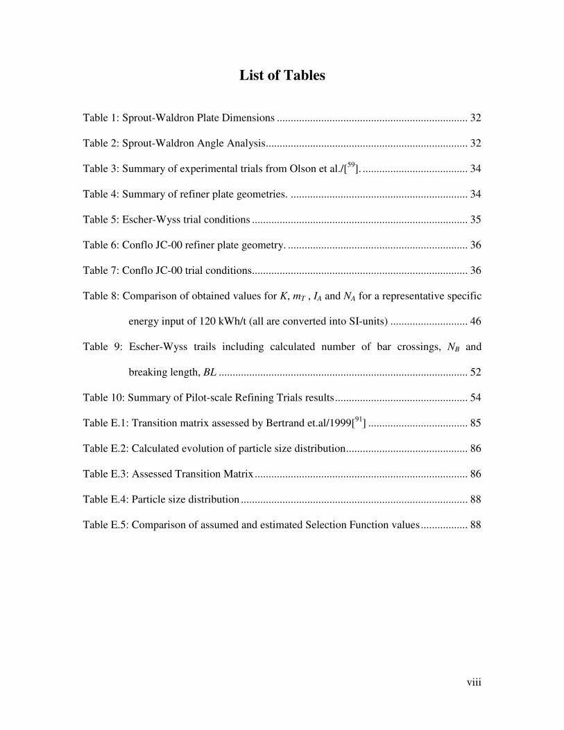
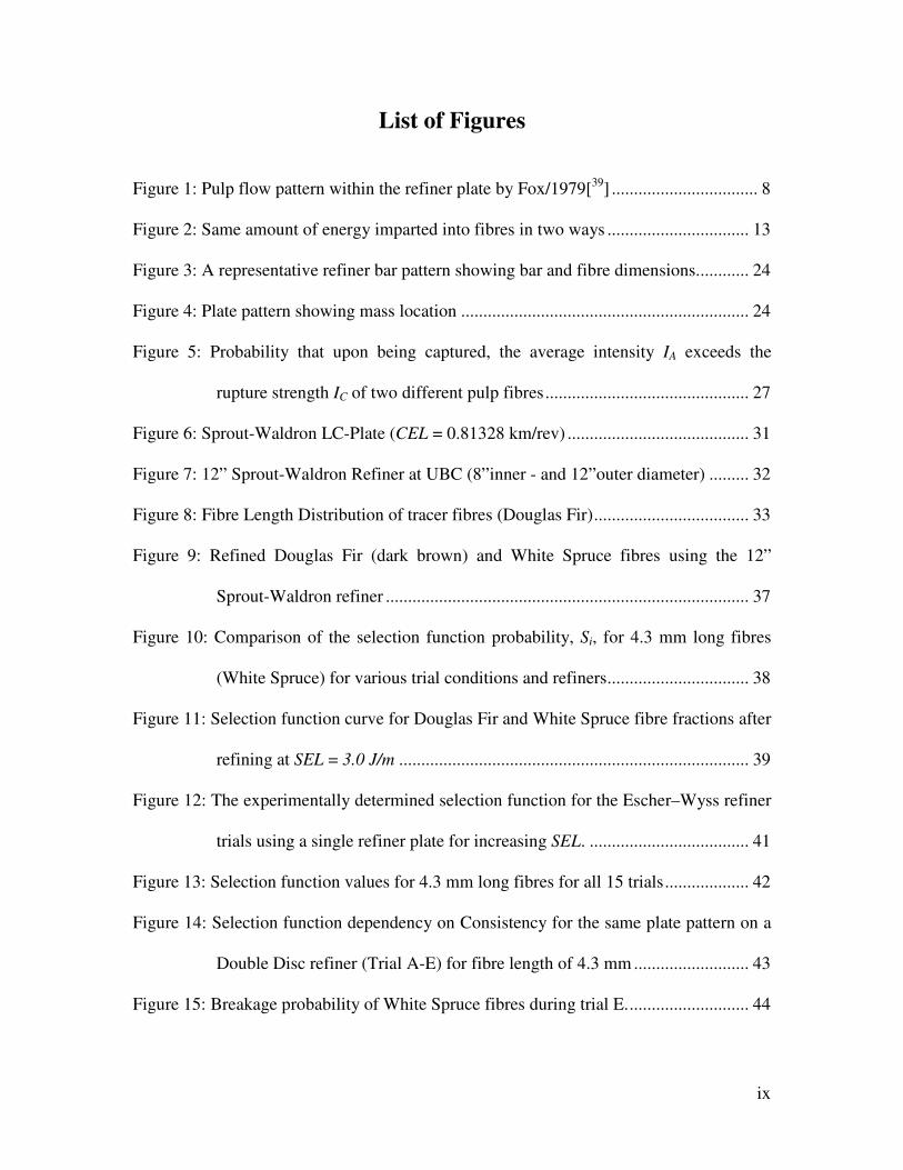
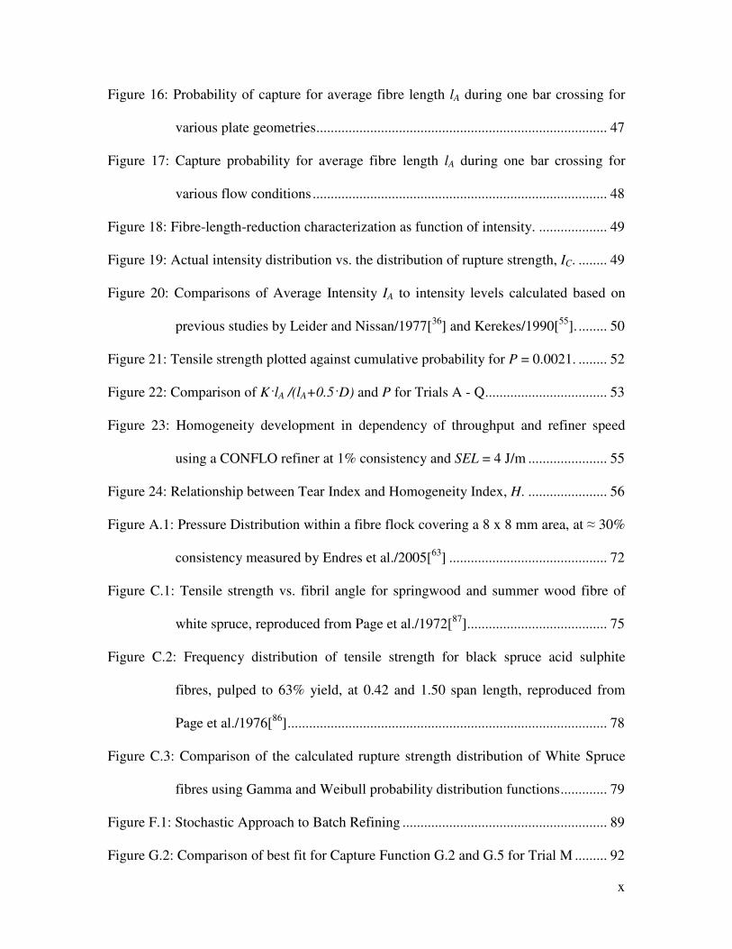
x
Figure 16 Probability of capture for average fibre length lA during one bar crossing for
various plate geometries 47
Figure 17 Capture probability for average fibre length lA during one bar crossing for
various flow conditions 48
Figure 18 Fibre-length-reduction characterization as function of intensity 49
Figure 19 Actual intensity distribution vs the distribution of rupture strength IC 49
Figure 20 Comparisons of Average Intensity IA to intensity levels calculated based on
previous studies by Leider and Nissan1977[36
] and Kerekes1990[55
] 50
Figure 21 Tensile strength plotted against cumulative probability for P = 00021 52
Figure 22 Comparison of KlA (lA+05D) and P for Trials A - Q 53
Figure 23 Homogeneity development in dependency of throughput and refiner speed
using a CONFLO refiner at 1 consistency and SEL = 4 Jm 55
Figure 24 Relationship between Tear Index and Homogeneity Index H 56
Figure A1 Pressure Distribution within a fibre flock covering a 8 x 8 mm area at asymp 30
consistency measured by Endres et al2005[63
] 72
Figure C1 Tensile strength vs fibril angle for springwood and summer wood fibre of
white spruce reproduced from Page et al1972[87
] 75
Figure C2 Frequency distribution of tensile strength for black spruce acid sulphite
fibres pulped to 63 yield at 042 and 150 span length reproduced from
Page et al1976[86
] 78
Figure C3 Comparison of the calculated rupture strength distribution of White Spruce
fibres using Gamma and Weibull probability distribution functions 79
Figure F1 Stochastic Approach to Batch Refining 89
Figure G2 Comparison of best fit for Capture Function G2 and G5 for Trial M 92
xi
Nomenclature
a Shape parameter for intensity distribution [kJkg]-1
A Comminution matrix
AF Cross sectional area fibre [m2]
b Scale parameter for intensity distribution [kJkg]-1
B Breakage function matrix
Bij Breakage function [-]
BL Breaking length of paper [km]
BEL Breaking Edge Length [km]
C C-Factor [s-1
]
CF Consistency pulp suspension [] or [-]
CEL Cutting Edge Length [kms]
E Energy input [kWht]
dE Incremental energy input [kWht]
D Groove Depth [mm]
EM Elastic Modulus (Youngrsquos modulus) [Pa]
f(li) Probability of capture form of fibres of length li [-]
FCi Factor for fibres length i to be captured during one bar crossing event [-]
Fmax Maximum force [N]
G Groove width [mm]
H Homogeneity index [-]
I Intensity of impacts [kJkg]
xii
IA Average intensity of impacts [kJkg]
IC Critical rupture strength of fibres [kJkg]
ICA Average critical rupture strength of fibres [kJkg]
In Identity matrix
K Empirical constant depending on machine parameter [-]
lA Average fibre length [mm]
mamp Mass throughput of OD pulp [th] or [kgs]
mG Mass of fibres in the grooves per unit bar length [kgm]
mT Mass of fibres in the gap per unit bar length [kgm]
MEL Modified Edge Load [Jm]
n(E) Column vector of fibre length classes at energy input level E
ni Numbers of fibre length class i [-]
dnini Incremental shortening of fibres of length class i [-]
nTracerj(E) Fraction of the number of tracer fibres in length class j [-]
nt Initial state vector
N Number of impacts on fibre [-]
NA Average number of impacts [-]
NB Number of bar crossings fibre experiences while traveling thr refiner [-]
NC Number of compression cycles [-]
outi Estimated values according to Markovian transition matrix approach
P Average probability of fibre capture for one bar crossing [-]
pC(IC) Rupture strength - probability distribution density function [-]
pI(I) Intensity probability distribution density function [-]
xiii
PR Probability of refining intensity exceeding the rupture strength of fibres [-]
pGamma(I) Gamma probability distribution density function [-]
Pnet Net energy input [kW] or [kJs]
Q Volume throughput [m3s]
R1 Inner radius refiner [m]
R2 Outer radius refiner [mm]
RBA Relative Bonded Area [-]
RD(E) Matrix of eigenvalues
R(NB) Fraction of fibres that have been captured and therefore treated [-]
S Selection function matrix
Si Selection function [kWht]-1
or [kJkg]-1
SEL Specific Edge Load [Wsm] or [Jm]
SRE Specific Refining Energy [kWht] or [kJkg]
SSL Specific Surface Load [Wsm2] or [Jm
2]
t Energy state [kWht] or [kJkg]
t(j i) Probability transition matrix
TEA Tensile energy absorption [Jm2]
UT Matrix of the eigenvectors
vij Elements of V(E)
Vamp Volume flow through the refiner [m3s]
V(E) Transition matrix
w Fibre coarseness [mgm]
WR Bar Width of the Rotor [mm]
xiv
WS Bar Width of the Stator [mm]
x Number of Bins of fibre length measurement [-]
α Shape parameter for gamma distribution function [-]
αB Bar angle [deg]
β Scale parameter for gamma distribution function [-]
δE Small energy input [kJkg]
ε Elastic strain at failure [-]
θ Sector angle refiner plate [-]
k Shape parameter for Weibull probability distribution function [-]
λ Scale parameter for Weibull probability distribution function [-]
micro Learning rate parameter
ρ Density fibre [kgm3]
σ Stress (tensile strength) [Nm2] or [Pa] or [10
1 dynecm
2]
υ Poisson ratio [-]
φ Bar angle [deg]
ω Rotational speed [revmin] or [revs]
xv
Acknowledgments
I would like to thank my supervisors James Olson and Richard Kerekes for providing
strong leadership inspiration and support over the course of my PhD and for showing
me what it takes to bring an academic quest through to completion I would also like to
thank my committee members Mark Martinez and Chad Bennington for their help and
advice in this project I wish also to acknowledge my co-researchers and staff of the pulp
and paper centre at UBC for their work ethic and encouragement namely Sean Delfel
Paul Krochak Tim Paterson and Ken Wong
It was absolutely necessary to have a supportive network of friends and family to help me
on my journey through this project My deepest thanks to those in my life who always
supported and encouraged me over the past years
Grateful acknowledgement is made for financial and technical support from NSERC
CANFOR STORA ENSO and FPInnovations Paprican Division
Chapter 1 Introduction
1
1 Introduction
Pulp refining is one of the most important unit operations in papermaking Its purpose is
to modify fibre morphology in order to improve paper properties by a technology which
has developed from batch beaters in the early 19th
century to flow-through disc conical
and cylindrical refiners in use today In pulp refiners fibres are trapped in the gaps
between bars during bar crossings during pulp flow through an annulus between a rotor
and stator which have bars on their surfaces and subjected to cyclic compression and
shear forces which modify fibre properties
The result of refining is changes in physical and optical properties of paper have been
studied in detail by various authors over the past decades (Higgins and de Yong1962[1]
Page1985[2] Seth1996[
3] and Hiltunen et al2002[
4]) to name only a few) It has been
generally found that within the commercial range refining increases tensile strength
(about threefold) burst strength folding endurance and sheet density whereas it reduces
tear strength of paper and sometimes fibre length
Although there is extensive literature on changes in fiber morphology produced by
refining there is relatively little on how the refining action takes place that is on the
refining process itself (Atack1980[5] Page1989[
6]) Consequently quantitative
characterization of refining action is limited The most widely used quantitative measure
of refining action is net energy expended per unit mass ie specific refining energy
(SRE) In addition it is common to use a ldquorefining intensityrdquo which reflects the energy
expended per loading cycle at each bar crossing event However although useful energy-
based characterizations have limitations because most changes within fibres occur as a
Chapter 1 Introduction
2
result of forces not energy The use of force in characterizing refining action has only
recently been undertaken (Kerekes and Senger2006[46
])
It has long been known that refining is very non-uniform in its treatment of pulp
(Danforth1986[7]) However the causes and consequences of this heterogeneity have
been little studied Furthermore heterogeneity of treatment has not been taken into
account in any of the refining theories or characterizations due in good part to a lack of
means to measure heterogeneity Thus it is reasonable to expect that a better
understanding of the nature of heterogeneity in refining will lead to a better
understanding of the process and perhaps offer a basis for improved technology
The objective of this dissertation is to develop a method to measure heterogeneity of
treatment in operating refiners
Chapter 2 Review of Literature
3
2 Review of Literature
Several excellent reviews of pulp refining have been produced over the years Generally
they have emphasized changes in fibre morphology caused by refining for example
Higgins and de Yong1962[1] Page et al1962[
8] Atack1977[
9] Page1985[
2]
Seth1996[3] and Hiltunen et al2002[
4]) The fundamentals of the refining process have
also received study as shown in the reviews of Ebeling1980[10
] Page1989[6]
Hietanen1990[11
] and Hietanen and Ebeling1990[12
]) The following review of the
literature will focus on highlights from past studies relevant to heterogeneity of treatment
21 Effect on Pulp
The main effects of refining on pulp are internal fibrillation external fibrillation fibre
shortening and fines generation More recently fibre straightening has been recognized as
another primary effect by Page1985[2] Mohlin and Miller1995[
13] and Seth2006[
14]
These outcomes of refining are described below in more detail
211 Internal Fibrillation
Measurements by Mohlin1975[15
] Kerekes1985[16
] and Paavilainen1993[17
] have
shown that refining chemical pulp increases fibre flexibility This occurs from
delamination in the cell wall which lowers its effective elasticity Water is drawn into the
fibre walls by capillary forces causing swelling which is often used as an indicator of
degree of refining The weakened cell wall is more flexible and collapsible thereby
giving a larger relative bonded area in paper This in turn increases bonding and thereby
paper strength
Chapter 2 Review of Literature
4
212 External Fibrillation
Another effect in commercial refining is the delamination of fibre surfaces called
external fibrillation This can be defined as a peeling off of fibrils from the fiber surface
while leaving them attached to the fiber surface (Page et al1967[18
] Page1989[6])
Clark1969[19
] emphasized that the fiber surface can be fibrillated even in the early
beating stage and that the external fibrils serve as bonding agents for inter-fiber bonding
The amount of such fibrillation (parts of fibre wall still attached to fibre) can be
quantified by measuring the increase in the specific surface of the long fibre fraction
(Page1989[6]) Although external fibrillation was studied from the earliest years of
refining because it was easily observable under microscope and was thought to be the
dominant result of refining several modern authors ie Page1985[2] and
Hartman1985[20
] concluded that external fibrillation has only limited effect on the tensile
strength or elastic modulus
213 Fibre Shortening
Refining causes fibre shortening which is generally undesirable in refining In some rare
applications it is a desired effect to improve formation by decreasing the crowding
number (Kerekes1995[21
]) In early work Page1989[6] showed that the mode of fibre
shortening was tensile failure rather than ldquocuttingrdquo by scissor-like shearing
214 Fines Generation
Fines meaning loose fibrous material of size less than 03 mm are produced in refining
as a result of fibre shortening or removal of fibrils from fibre walls According to
Chapter 2 Review of Literature
5
Page1989[6] generated fines consist mostly of fragments of P1 and S1 layers of the fibre
wall due to the abrasion of fibres against each other or against refiner bars
215 Fibre Straightening
Fibre straightening is considered an important refining effect (Page1985[2]
Mohlin1991[22
] Seth2001[23
]) If fibres remain curly or kinked in a paper network they
must be stretched before they can carry load meaning that fewer fibres carry load during
the initial stretching of paper and therefore paper is weak Fibre straightening permits
fibre segments between bonded sites in paper to be ldquoactiverdquo in carrying load The
mechanism by which refiners straighten fibres is likely due in part to tensile strain in
refiner gaps and by causing fibre diameter swelling In the latter case upon drying
shrinkage of swollen fibres stretches fibres segments between bonded sites and thereby
straightens them
216 Heterogeneity
It has long been known that refining is a heterogeneous process and that the resulting
heterogeneity affects paper properties One of the earliest workers to show this was
Danforth1986[7] by mixing of fibres subjected to differing levels of refining Larger
heterogeneity gave poorer properties eg lower tensile strength Others have shown
heterogeneity by observations of morphology changes (Page1989[6]) The literature on
heterogeneity will be reviewed extensively later in section 26
22 Mechanics of Refining
Current knowledge of the mechanics of refining is far less than is knowledge of the
refining result The design of refiners is largely empirical In addition to action on pulp
Chapter 2 Review of Literature
6
design is based on factors such as sufficient groove size to permit flow of the fibre
suspension through the machine bar wear and material cost Scientific studies of the
process of refining have been carried out by various researchers Some highlights of this
past work are described below
221 Fibrage Theory
Smith1922[24
] proposed that a refiner bar moving through stock collects a ldquobeardrdquo or
fibrage of fibers on the leading edge This capture of fibre transports fibres into the gap
between rotor and stator bars A study of the compressive and shearing forces exerted on
the bars during refining by Goncharov1971[33
] gave some support to the fibrage
mechanism
222 Refining as Lubrication Process (Hydrodynamics)
Rance1951[25
] and Steenberg1951[26
] analyzed refining as a lubrication process Their
experiments offered indirect evidence of the occurrence of (a) fluid (hydrodynamic)
lubrication (b) boundary lubrication and (c) lubrication breakdown which produced
excessive metal wear in the refiner Steenberg1951[26
] carried out his experiments with a
Valley beater varying the consistency load and peripheral speed He concluded that
Valley beating is carried out under hydrodynamic (fluid) lubrication conditions and that
the work absorption capacity ie coefficient of friction decreases with beating as does
the apparent viscosity of the pulp More recently Frazier1988[27
] applied the lubrication
theory to refiner mechanical pulping and derived an expression for the shear force applied
to pulp Similarly Roux1997[28
] performed a lubrication analysis in order to characterize
hydrodynamic forces in refining Based on experiments Lundin et al1999[29
] propose
Chapter 2 Review of Literature
7
that the power consumption in refining is governed by a lubrication film between the
rotor and the stator Although characterization of the refining process as a hydrodynamic
phenomenon has yielded some useful correlations treating the fibre suspension as a fluid
has some serious limitations Refiner gaps are 5-10 fibre diameters deep and therefore the
water-fibre suspension in a gap is not a continuum Consequently the suspension in the
gap does not meet a primary property of a fluid
223 Transport Phenomena in Refiners
Flow behavior in refiners has been examined by several workers Complex flow patterns
have been observed and residence time distributions have been measured using high
speed photography (Halme and Syrjanen1964[30
] Herbert and Marsh1968[31
]
Banks1967[32
] Gonchorov1971[33
] Fox et al1979[34
] and Ebeling1980[10
]) Halme
and Syrjanen1964[30
] Herbert and Marsh1968[31
] observed that pulp flows primarily in
the radial direction outward in the grooves of the rotor and inward in the grooves of the
stator Other recirculation flows called secondary and tertiary flows are also present in
disc refiners Fox et al[34
] proposed that the secondary flows arise from the motion of the
land area of the bars passing over the grooves and that tertiary flows result from the
difference in static pressure between opposing grooves of the rotor and stator (see Figure
1) Using a material and energy balance Leider and Rihs1977[35
] and Leider and
Nissan1977[36
] related the pressure drop across the refiner to its volumetric flow rate
This accounts for the action of the centrifugal and frictional forces and is expressed in
terms of operating conditions fluid properties and plate properties
Chapter 2 Review of Literature
8
Figure 1 Pulp flow pattern within the refiner plate by Fox1979[3437
]
Arjas et al1969[38
] studied the effect of flow rate and angular velocity on the shape of
the residence time distribution curve They concluded that the flow rate has an effect on
the mean residence time but the effect of the angular speed is not very large
224 Treatment of Flocs Hypothesis
Page et al1962[8] showed that flocs rather than individual fibres are treated in refining
although it is possible that fibers may be oriented in a floc network to receive fiber
treatment From high-speed photography of a conical refiner they concluded that a
refiner is inefficient since only a small proportion of fibers are subject to treatment Page
et al1962[8] Hietanen and Ebeling1990[
12] found that flocculation plays an important
role in low-consistency refining Similarly studying power and gap size relationships
Batchelor amp Ludin2006[39
] estimated the fraction of bar length covered with fibres
Banks1967[32
] proposed a detailed picture of refining action based on floc treatment in
contrast to the fibrage theory which assumes a uniform coverage of the bar edges by
Tertiary Flow
Rotor
Stator
ω
Primary Flow Secondary Flow
Chapter 2 Review of Literature
9
individual fibres He summarized the mechanics of refining based on observations using
high-speed photography
1 Flocs consolidate when they are trapped between approaching tackle elements
2 Mechanical pressure induced by the tackle elements becomes high enough and
causes plastic deformation in the fibers composing the floc Consolidation
continues
3 The floc compressed between the bars is sheared flocs (and fibers) are
ruptured
4 Release of mechanical pressure allows absorption of water to take place into
the ruptured fibrils and fibers
5 Turbulent agitation may disperse the floc or its remnants into the general mass
flow
225 Refining as a Fatigue Process
Fibres may be exposed to many bar crossing events during their passage through a
refiner Thus fibres are likely to experience multiple loading cycles Page et al1962[8]
and Atack1977[9] suggested that this repeated straining causes fatigue weakening of the
fibres and this in turn produces internal fibrillation On the other hand fibre shortening
(cutting) is likely to be caused by one severe loading cycle Page1989[6] suggested
rupture takes place by tensile failure rather then a scissor-like cutting action Kerekes and
Olson2003[40
] proposed that fibre rupture in refiners is caused by a single event rather
than fatigue process
Another approach to account for the cyclical nature of the process was proposed by
Steenberg1979[41
] He considered the refining process to be an irreversible kappa
Chapter 2 Review of Literature
10
process in which there is a critical path for the formation of a stress concentration chain
which causes a structural breakdown For another structural breakdown to occur the
particles ie fibers need to be rearranged Thus cyclicality is needed to overcome
heterogeneity Most recently Goosen et al2007[42
] examined the role of fibre
redistribution in pulp refining by compression They concluded that the role of cyclic
loading is to expose new fibres to loading cycles rather than to produce fatigue
weakening In essence cyclicality in the process is to overcome heterogeneity rather then
to produce fatigue weakening
226 Forces on Fibres during Bar Crossing Events
A number of studies have examined the manner in which forces are imposed on fibres
within refiner gaps Page 1989[6] suggested that refining should be quantified by the
stresses and strains applied to fibres These stresses and strains are caused by bar forces
which have been the subjects of several studies
Goncharov1971[43
] was the first to measure pressures on refiner bars during bar crossing
events Later Martinez et al1997[44
] and Batchelor et al1997[45
] analyzed the
compressive and shear forces action on single flocs and measured normal and shear
forces in a ldquosingle barrdquo refiner apparatus Kerekes and Senger[46
] developed equations
for bar forces and fibre forces from the specific edge load (SEL) Page1989[6] Martinez
et al1997[44
] and Koskenhely et al2007[47
] addressed issues concerning the bar edge
force
Chapter 2 Review of Literature
11
23 Quantitative Characterization of the Refining Mechanism
As described earlier specific refining energy is the most common quantitative
characterization of refining action This energy is factored into the number of impacts
imposed on pulp and the intensity of each impact ie loading cycle Most intensities are
based on energy per loading cycle though in recent work Kerekes and Senger2006[46
]
have proposed a force-based intensity These concepts are described in detail below
231 Specific Energy
Specific refining energy (SRE) is the useful energy imparted to the pulp suspension ie
the total energy less the no-load energy It is obtained by dividing the net power input
into the refiner by the fibre mass throughput
ρsdotsdot==
VC
P
m
PSRE
F
netnet
ampamp
(1)
The typical range for SRE in chemical pulp refining is between 80 to 250 kWht
depending on the furnish and the desired papermaking property
232 Refining Intensity
The major means of characterizing refining intensity today is by a ldquomachine intensityrdquo
meaning an intensity which reflects energy expended per bar crossing without direct
reference to how this energy is expended pulp The most common such method is the
Specific Edge Load (SEL) This was introduced by Wultsch and Flucher1958[48
] and
developed further by Brecht and Siewert1966[49
] who demonstrated the dominant impact
of the bar edge The SEL is determined by the net power divided by the bar edge length
(BEL) multiplied by the rotational speed ω The BEL is determined by multiplying the
Chapter 2 Review of Literature
12
number of bars on stator by the number of bars on rotor by the refining zone length The
result is expressed in Wsm or Jm The expression for SEL is
CEL
P
BEL
PSEL netnet =
sdot=
ω
(2)
int sum∆sdot
congsdotsdot
=2
11 coscos
R
R
Nsrsr rnnrnn
BELθθ
(3)
An extension of the SEL the specific surface load (SSL) was suggested by
Lumiainen1990[50
] to account for bar width rather than just bar edges This was
accomplished by including bar width W with the SEL thereby giving the area of the bars
and units Wsm2 or Jm
2
( )
sdot
+sdotsdot
=
2cos2 B
SR
net
WWCEL
PSSL
αω
(4)
Using this approach Lumiainen distinguished between refiner plates having identical
cutting edge length (CEL) but differing bar widths
Meltzer and Rautenbach1994[51
] used the ldquocrossing speedrdquo ndash which is a measure of fibre
treatment frequency by calculating the crossing speed per dry fibre mass flow ndash to further
modify the SEL-concept This gave the modified edge load (MEL) which accounts for bar
width W groove width G and the average intersecting angle of rotor and stator bars For
identical rotor and stator geometry the following expression was derived
W
GWSELMEL
B
+sdot
sdotsdot=
αtan2
1
(5)
The factor W+G W considers the refining work of the bar surfaces and the probability of
fibre treatment received
Chapter 2 Review of Literature
13
233 Fibre Intensity
The above characterizations based on energy per bar crossing are ldquomachine intensitiesrdquo
that make no direct link to the pulp in the refiner To make this link characterizations
have been developed that factor SRE into two quantitative parameters the number of
impacts N and the intensity of each impact I on pulp In this case I is a ldquofibre
intensityrdquo The product of these in the SRE are shown in equation (6)
INSRE sdot= (6)
Figure 2 Same amount of energy imparted into fibres in two ways
As shown in Figure 2 differing combinations of N and I give differing refining results
Because only 2 of the variables in equation (6) are independent it is common to use SRE
and I Lewis and Danforth1962[52
] and later Danforth1969[53
] defined expressions for N
and I but these were empirical in nature and did not rigorously represent N as a
dimensionless variable and I as energy per bar per impact
Number of impacts N
Inte
nsi
ty o
f im
pac
ts
I
Fibre cutting
Fibre straightening
Fibrillation
SRE1 = SRE2
SRE1
SRE2
Chapter 2 Review of Literature
14
Van Stiphout1964[54
] calculated the probability of a fibre being caught in the refiner gap
Based on this he was able to estimate the forces acting on fibres and the mass of fibres
being treated per length of bar According to his analysis the mass of fibres per bar length
was proportional to the mean residence time He further postulated that the damaging
affect of refining was proportional to the surface sheared and that the net power was
active on an amount of fibres enclosed in the gap between the refiner bars However two
empirical parameters of unknown magnitude limited the application and scientific
meaning of this work
Leider and Nissan1977[36
] were the first to derive equations for N and I in rigorous
terms They represented the probability of a fibre being stapled on a bar by fibre length
and diameter to give an estimate of ldquonumber of impacts per single fibre per refiner passrdquo
Another approach to define values for N and I to overcome some of the shortcomings of
Leider and Nissan was made by Kerekes1990[55
] in the form of the C-factor
C
P
m
CIN
m
PSRE netnet sdot=sdot==
ampamp
(7)
In this approach C is defined as the capacity of a refiner to inflict impacts (loading
cycles) on fibres Kerekes1990[55
] derived equations for the C-factor as a function of
plate geometry (bar width depth length angle and edge geometry) speed consistency
fiber length and coarseness The C-factor for a disc refiner for a simplified case (small
gap size similar bar pattern on rotor and stator) is given by
( )( )( )Dlw
RRnlCGDC
A
AF
+
minus+sdot=
3
tan218 3
1
3
2
32 φωρπ
(8)
A crucial assumption of the analysis is estimating the probability of fiber contact with the
leading edge of the bar which he expresses as l (l + D+ T) Kerekes showed that this
Chapter 2 Review of Literature
15
assumption led to logical outcomes at the limits of bar size relative to fibre length The C-
Factor analysis is perhaps the most rigorous and comprehensive theory developed to date
It has been applied to a variety of refiner geometries including the disk conical and PFI
mill It takes into account factors relating to bar and groove geometry as well as fibre
length which provide a more accurate description of refining intensity However the C-
factor predicts only average values rather than distributions of intensity
24 Heterogeneity
It has long been accepted that refining is a heterogeneous process (Page1989[6]) The
sources of heterogeneity are numerous ranging from the mechanism of transferring
mechanical forces into fibers (Steenberg1963[56
]) to the irregular flow pattern through
the refiner (Halme1962[57
])
There are also scales of heterogeneity ranging from large to small Ryti and
Arjas1969[58
] studied the large distributions of residence time in refiners originating
from large scale secondary flows They postulated that greater uniformity in refining
treatment gives a better refining result They concluded that the refining action is related
to the residence time inside the refiner and to the probability of treatment during this
time Fox et al1979[34
] studied flow in a small disc refiner by visual observation They
found that after being ldquoreleasedrdquo from a gap fibres either become part of the stator flow
towards the refiner axis and stapled again on a bar or become part of the outward rotor
flow leaving the refiner In addition fibres may flow back to the stator from the outside
annulus of the refiner This all resulted in a poor pulp circulation and therefore limited the
amount of fibres receiving treatment in refiner gaps
Chapter 2 Review of Literature
16
Additional sources of heterogeneity arise from a finite probability of capture from the
groove (Olson et al2003[59
]) fractional bar coverage (Batchelor and Ludin2006[60
])
non-uniform force distribution within flocs (Batchelor and Ouellet1997[61
]) non-
uniform SEL along the radius of the refiner (Roux and Joris2005[62
]) non-homogeneous
force distribution on fibre networks while being under load (Endres et al2005[63
]) and
out-of-tram of rotors (Prairie et al 2007[64
]) An added complexity is the wide variability
of fibre properties in any pulp It is well known that species pulp type bleaching process
and the relative amounts of thick and thin walled fibers can affect refining Page1983[65
]
has suggested that differences in the beatability and refining action of kraft and sulfite
pulps are due to differences in their viscoelastic behavior Yet another factor is fibre
flocculation Hietanen and Ebeling1990[12
] Hietanen1991[66
] and Lumiainen1995[67
]
have all suggested that flocculation is a major source of refining heterogeneity
Various studies have been conducted to measure heterogeneity of treatment in refining
Simons1950[68
]) used a staining technique to identify damaged fibres Nisser and Brecht
1963[69
] evaluated refining heterogeneity by calculating the swollen length of fibres
before and after refining Another approach has been to examine physical changes in
fibres Mohlin and Librandt1980[70
] using SEM technique found that one of the major
differences between laboratory refining and production refining is the homogeneity of
treatment Dahrni and Kerekes1997[71
] measured deformations in plastic tracer fibres
They found that 30 of the fibre passed through a lab disc refiner with no visible sign of
impact whereas other fibres were severely deformed Dekker2005[72
] measured the
changes in RBA of fibres by quantifying the optical contact between fibres and a glass
slide He found that only 7-20 of fibres were treated
Chapter 2 Review of Literature
17
Another approach for measuring heterogeneity is based on comparing properties of
papers made from mixtures of unrefined and well-refined pulp (Dillen1980[73
]) As a
measure of the heterogeneity he used the coefficient of variation of the amount of
refining Lastly Hietanen1991[66
] found that the homogenizing effect of deflocculation
has a positive impact on paper strength properties
In summary the sources of heterogeneity in refining are many and there are some
methods to measure it but no existing methods are suitable for measurement of
heterogeneity of treatment in operating refiners
25 Review of Refining Action as a Comminution Process
Comminution is defined as the reduction of particle size by mechanical processing
Models for the comminution process models were developed for crushing and grinding in
the powder industry 60 years ago to predict particle size distribution changes during
processing The basics were developed by Epstein1948[74
] Reid1965[75
] and
Austin1971[76
] They modeled batch grinding by the introduction of two statistical
functions a Breakage function Bij and a Selection function Si Basically Si represents
the probability of a particle of size i per unit time or energy and has the units of time-1
or
energy-1
The breakage function Bij represents the probability of particles larger than i
being reduced to size i As the particle size can only be reduced during grinding the
values of Bij are dimensionless and range between 0 and 1
The incremental change in the number of fibres of length i dni per incremental applied
energy dE is given by the comminution equation shown below
Chapter 2 Review of Literature
18
jj
ij
ijii
i nSBnSdE
dnsum
gt
+minus= (9)
Applied to refining ni represents the number of fibres of length i available for cutting Si
is the selection function for fibres of length i per unit energy The product of Si and ni
represents the decrease in number of fibres of length i The term ΣBijSjnj represents the
increase in the number of fibres of length i per unit energy from the cutting of fibres of
lengths larger than i
For refiners we may consider incremental energy to be the discrete event of a single bar
crossing assuming this to inflict a single loading cycle on fibres and fibres to be ruptured
by a single excessive loading cycle
Steenberg1963[56
] suggested that several sub-processes have a major influence on the
refining result during certain phases of refining Thus a single parameter cannot be used
to describe either the process or the state of the product (ie refined pulp) He suggested
that at least two of the sub processes namely the ldquoselection processrdquo and the ldquotreatment
processrdquo deserve more attention
Other workers applied the model directly to describe fibre length distribution changes
caused by refining for example Kane1957[77
] and Meyer et al1966[78
] Roux and
Mayde1997[79
] applied the comminution theory to analyze the change of the mean fibre
length during refining They predicted the potential for fibre cutting under given
conditions to be a function of the energy consumed by the solid phase and the average
impact intensity ie the ratio between the net machine power and the ldquocuttingrdquo length of
Chapter 2 Review of Literature
19
bars per unit time However their equations had inconsistent units making their results
difficult to interpret rigorously
Corte and Agg1980[80
] used a comminution model to compare the shortening rate of
fibres in a disc refiner and a laboratory beater They found that the disc refiners cut long
fibre more rapidly than short fibres while a laboratory beater cut long and short fibres at
the same rate Olson et al2003[59
] applying a technique developed by Koka and
Trass1988[81
] found that the probability of fibres being selected for cutting during
refining is proportional to the applied energy and fibre length and was independent of
consistency Regression fitting that minimizes the difference between measured and
predicted fibre length distributions was used to determine the selection function Si for
various pulp and refiner combinations
Several other investigators applied the comminution theory to the production of
mechanical pulp in chip refiners Corson1972[82
] modeled the refining of wood chips
into individual fibres using a comminution approach This approach was used more
recently in an expanded form by Strand and Mokvist1989[83
] to model the operation of a
chip refiner employed in mechanical pulping of wood chips
Chapter 3 Objective of Thesis
20
3 Objective of Thesis
The above review shows that there is a need for a rigorous practical method to measure
heterogeneity in operating refiners The objective of this thesis is to develop such a
method The approach is based on interpreting measurements of fibre shortening by a
model of the physical process of refining described by comminution theory
Chapter 4 Analysis
21
4 Analysis
Comminution modeling is a potentially useful basis for measuring heterogeneity for
several reasons Fibre shortening obviously reflects the probabilistic nature of refining
because some fibres are shortened while others are not The result decreased fibre length
is a measurable change for which instruments for rapid measurement are now available
Lastly the best tracer particles to reflect what happens to fibres are fibres themselves
Fibre shortening is generally not an objective of refining Indeed it is to be avoided in
most cases In this study fibre shortening will be used merely as an event to characterize
the mechanics of the process rather that as a desired outcome We employ comminution
theory as the scientific basis of our approach To do so we address several individual
problems
interpretation of comminution equation
link to refiner mechanics
probability of fibre capture in a gap
probability of fibre shortening in a gap
link between breakage function and selection function
Chapter 4 Analysis
22
41 Interpretation of Comminution Equation
As discussed earlier the comminution equation reflects the net change in the number of
fibres of size i as the result of the decrease size i caused by shortening and the increase
caused by fibre shortening from larger sizes
jj
ij
ijii
i nSBnSdE
dnsum
gt
+minus= (10)
However our specific interest in this work is only the shortening component of
comminution Therefore we focus on the first two terms of the comminution equation
We define the incremental shortening as dni to differentiate it from the net shortening
dni in equation (10) Rearranging terms we obtain
dESn
dni
i
i sdotminus=
(11)
In essence this equation relates the incremental fraction of fibres of length i (dni ni)
that are shortened to the product of the selection function Si and the incremental energy
supplied dE
We now consider SidE in terms of refiner variables specifically to fibre rupture during a
single bar crossing The probability of fibre rupture is the product of two other
probabilities a factor of fibre capture from the groove FCi and the probability that once
captured the fibre is ruptured PR We consider PR the probability that the intensity a
fibre sees is greater than its rupture strength (intensity) to be independent of fibre length
Thus we may express SidE as
RCii PFdES sdot=sdot (12)
We now link dE FCi and PR to refiner mechanics and thereby refiner variables
Chapter 4 Analysis
23
42 Link to Refiner Mechanics
We first link energy per mass supplied to a refiner E to the product of number of impacts
imposed on fibres N and the intensity per input I expressed as energy per mass
INE sdot= (13)
We may express this equation in incremental form as
dNIdINdE sdot+sdot= (14)
Assuming that for a given refiner the average intensity at bar crossings is constant and
represented by IA and since dI = 0 we obtain
dNIdE A sdot= (15)
421 Intensity
We now interpret N and IA in terms of measurable refiner variables at a single bar
crossing
Refining intensity is commonly defined by the Specific Edge Load (SEL) Kerekes and
Senger2006[46
] have shown that SEL represents the energy expended per bar crossing
per unit bar length Thus the average energy expended on fibre mass within the gap of a
bar crossing IA is given by SEL divided by the mass of fibres in the gap per unit bar
length mT ie
T
Am
SELI =
(16)
422 Number of Impacts
The number of impacts on pulp N is a function of the product of two factors the
probability of an impact at a single bar crossing and the number of bar crossings NB that a
Chapter 4 Analysis
24
fibre would experience if it passed along a stator bar during its residence time in the
refiner We can define a mass-average probability of impact at a bar crossing by the ratio
of the mass of pulp captured mT to the total mass associated with a bar crossing (pulp in
gap and pulp in adjacent groove mG) giving mT (mT + mG) Thus
( ) BGTT dNmmmdN sdot+= (17)
Figure 3 A representative refiner bar pattern showing bar and fibre dimensions
Figure 4 Plate pattern showing mass location
We assume that the consistency in refiner grooves equals the pulp suspension
consistency CF Thus
ρ x CG x D2 Fsdotsdot=Gm (18)
We may note here that the above equations give the following equation when combined
GT
B
T
B
GT
T
Amm
SELN
m
SELN
mm
mINE
+
sdot=sdotsdot
+=sdot=
(19)
These expressions represent averages We now consider distributions
Rotor
Stator
Tm
Gm
G D W
T Pulp fibre
Stator
Rotor
li
Chapter 4 Analysis
25
43 Fibre Capture Factor
The above mass-average probability of capture assumes a dependence only on mass ratio
However other factors also affect fibre capture For example the mass in a groove may
not reflect eligible fibres because there may be dead zones of inactive fibres stuck in the
groove This would be a source of heterogeneity In addition it has long been known
(Smith1922[24
]) that longer fibres tend to be more easily captured then short fibres
individually or as flocs To reflect these factors we express the factor of capture as a
probability based on fibre length f(li) and a constant K that reflects other unknown
factors influential in capture such as consistency rotational speed throughput and plate
geometry Clearly K falls in the range 0 le K le 1 Thus
)( iCi lfKF sdot= (20)
44 Probability Distribution of Intensity
Once in a gap fibres rupture when they experience a force exceeding their rupture
strength We consider forces to be represented by intensities expressed as energy per unit
mass Thus the probability of fibre rupture depends on the intensity applied to a fibre I
and the rupture intensity IC We further assume that once captured rupture is
independent of fibre length
We assume the distribution of intensity I on a pad of pulp to be similar to the spatial
pressure distribution measured by Endres et al2005[63
] In this work Endres measured
local pressure distributions on pads of wet pulp in increments of a few mm ie 8 x 8 mm
In a refiner gap compression forces are large about 10 times the shear forces (Prairie et
al2007[64
]) and therefore are likely to vary in a similar manner to the measurements of
Endres along bar length in gaps even in the presence of shear forces In the absence of
Chapter 4 Analysis
26
other information of local forces in refiner gaps we deemed this to be a reasonable
assumption As shown in Appendix B the intensity density distribution can be described
by Weibull function and more approximately by a simple form of the Weibull equation
the gamma density distribution as shown below
bI
I aIeIp minus=)( (21)
The constants a and b can be determined from two equations one normalizing the
distribution to 1 the other integrating the distribution multiplied by I to give the average
intensity IA as shown in Appendix B This gives
[ ]( )
II
A
IAIe
I
kgkJIp
sdotminus
sdotsdot
=
2
2
14)( where TA mSELI =
(22)
The strength of fibres IC also has a distribution We represent this distribution as pC(IC)
As shown in Appendix C this too can be represented by a Weibull density distribution
We now relate PR in equation (12) to above probabilities Clearly rupture occurs when
the applied intensity I equals or exceeds fibre rupture intensity IC summed over all fibre
rupture intensities This is given by
( ) ( ) CCC
I
IR dIdIIpIpP
C
sdotsdotsdot= int intinfin infin
0
(23)
Solving the double integral of equation (23) does not give a simple general analytical
solution owing to the complexity of the probability distribution functions in use pI(I) as a
Gamma density distribution function and pC(IC) as a Weibull density distribution
function It has the form
( )( )
C
A
I
I
AC
CCR dII
eIIIpP
A
C
sdotsdot+sdot
sdot= intinfin
sdotminus
0
2
2
(24)
Chapter 4 Analysis
27
( )C
A
I
I
AC
I
k
CkR dII
eIIeI
kP
A
Ck
C
sdotsdot+sdot
sdotsdotsdot= intinfin
sdotminus
minus
minus
0
2
1 2λ
λ
(25)
The solution of equation (25) is a hyper geometric function for which examples for two
different rupture strengths are shown Figure 5
000
010
020
030
040
050
060
070
080
090
100
0 10 20 30 40 50 60 70 80 90 100
Average Intensity IA [kJkg]
Pro
bab
ilit
y o
f R
up
ture
P
R [
-]
= 35 kJkg
= 25 kJkg
( ) ( ) ( ) CCC
I
ICRR dIdIIpIpIIPP
C
sdotsdotsdot== int intinfin infin
0
[ ]( )
II
A
IAIe
I
kgkJIp
sdotminus
sdotsdot
=
2
2
14)(
( )
k
CI
k
CkCC eIk
Ip
minus
minussdotsdot= λ
λ
1
I CA
I CA
Figure 5 Probability that upon being captured the average intensity IA exceeds the
rupture strength IC of two different pulp fibres
45 Selection Function Expressed in Terms of Refiner Variables
We now link the above probabilities to the selection function Si We do so by
substituting FCi from equation (20) and PR from equation (23) into equation (12) We
obtain dE by substituting in equation (15) for IA from equation (16) and for dN from
equation (17) Assuming mT laquo mG (Batchelor and Lundin2006[60
]) and considering 1 bar
crossing to be dNB = 1 we obtain
Chapter 4 Analysis
28
( ) ( ) ( ) CCC
I
I
G
ii dIdIIpIpSEL
mlfKS
C
sdotsdotsdotsdotsdotsdot= int intinfin infin
0
(26)
Equation (26) contains three unknowns mT K f(li) These parameters are determined
from Si of the comminution equation However first the relationship between Si and Bij
must be established
46 Relationship between S and B
An analysis relating S and B is shown in Appendix D In brief we first determined a
suitable breakage function to represent probabilities of rupture anywhere along a fibre
length (Olson et al2003[59
]) Previous work by others eg Corte et al1980[80
] assumed
that fibres shortened into only two parts of varying length Our analysis has no such
restriction We determined Bij for a rupture at any point by introducing matrix A that links
Bij and Si giving equation (9) in matrix form as shown below
nAdE
dnsdot= where ( ) SIBA n sdotminus=
(27)
Variable n(E) is a column vector whose entries are the fibre mass fraction in each size
interval after the energy input dE We solved equation (9) by diagonalization of A and
introducing UT as the matrix of the eigenvectors Assuming the process to be Markovian
we re-expressed the population balance as ni(after)=V(E)middotni(before) following the
procedure of Berthiaux2000[84
] We thus decompose V into its characteristic roots
which represent the eigenvalues exp(-SimiddotE) From the matrix of the eigenvectors we
obtained A and from equation (27) the breakage function Bij Further details on this
analysis are given in Appendix D
Chapter 4 Analysis
29
47 Curve -Fitting Procedure
Lastly we selected an appropriate procedure for regression fitting data in fibre length
changes before and after refining to equation (26) to obtain Si We accomplished this in
using GaussndashNewton algorithm method in two steps
First we determined the functional form of the parameter f(li) assuming it to depend on
fibre length alone and to be independent of mT and K This was accomplished by fitting
curve shapes of Si vs fibre length
Next having obtained the form of f(li) we determined parameters mT and K
simultaneously by regression fitting to equation (26) This was accomplished by the same
regression fitting method
Chapter 5 Experimental Program
30
5 Experimental Program
Our experimental program consisted of analyzing fibre length reductions produced by
various refiners We used MatlabTM
software coded to calculate simultaneously the
selection and breakage function for different refining conditions Fibre length
distributions before and after refining were measured using a Fibre Quality Analyzer
(FQATM
) The instrument gives fibre length histograms which contain approximately 150
bins with length increments equal to 005 mm In order to reduce the sampling noise and
the large time associated with calculating a 150 x 150 element transition matrix and
within it the S and B matrix the measured fibre length distributions were compressed into
20 bins with an increment of 025 mm and then normalized Fibres shorter than 05 mm
were included in the measured distributions of this study in contrast to the approach of
Olson et al2003[59
] This may introduce an error because short fibres and fines can be
generated by peeling off pieces of fibre wall rather than by fibre shortening However in
this study all fibres were treated as being a result of fibre shortening The influence of
fines on the overall outcome of the parameter calculation was investigated
The experimental work was carried out in the steps shown as below
Validation of the comminution approach
Evaluation of data from industrial scale pilot plant trials
Evaluation of data from laboratory refiners
Chapter 5 Experimental Program
31
51 Validation of Comminution Approach
The aim of this portion of the experimental work was to validate the comminution
approach by a simple case of comminution examined by Berthiaux2000[84
] described in
Appendix F This was accomplished by employing an easily detectable tracer fibre in
pulp The tracer fibre was a laboratory-produced Douglas Fir pulp cooked using the
ldquokraftrdquo process to an H-factor of 1600 The resultant pulp was carefully washed and later
classified three times in accordance to TAPPI test method T233 cm-95 with the Bauer-
McNett classifier Only the R14 long fibre fraction of the original pulp was retained and
further classified to obtain a narrow distribution (3-4 mm) of long fibres as the tracer As
a result of this procedure we obtained a nearly perfect defect-free pulp having a narrow
length distribution as shown in Figure 8
Figure 6 Sprout-Waldron LC-Plate (CEL = 081328 kmrev)
For the validation a pulp mixture (2 Douglas Fir tracer fibre and 98 White Spruce)
was circulated through a single-disc refiner shown in Figure 7 The flow loop consists of
two large 455 liter plastic tanks a 20 HP centrifugal pump and a PVC pipe network that
circulated the pulp from one tank through the refiner and into the second tank (or into the
Chapter 5 Experimental Program
32
same tank for batch refining) The pulp suspension of 3 was refined at a target SEL of
3 Jm at 600 rpm up to a SRE of 240 kWht
Bar Width
[mm]
Groove Width
[mm]
Groove Depth
[mm]
G Base Radius
[deg]
Draft Angle
[deg]
29 28 28 05 3
Table 1 Sprout-Waldron Plate Dimensions
Nominal Angle
[deg]
Cluster Angle
[deg]
Avg Int Angle
[deg]
Groove Volume
[cu cmcm]
10 225 465 0566
Table 2 Sprout-Waldron Angle Analysis
Figure 7 12rdquo Sprout-Waldron Refiner at UBC (8rdquoinner - and 12rdquoouter diameter)
Chapter 5 Experimental Program
33
Pulp samples were obtained at energy increments of 30 kWht From the samples of
refined pulp approximately 100 tracer fibres were collected by pipette under a
microscope The sampling procedure was repeated 30 times in order to obtain a sufficient
amount of fibres for measurement of fibre length in the Fibre Quality Analyzer (FQA)
0
2
4
6
8
10
12
0 1 2 3 4 5 6 7 8 9 10
Fibre length [mm]
Fre
qu
en
cy [
]
DF - originalR14 (1 x Fractionation)R14 (2 x Fractionation)R14 (3 x Fractionation)
Figure 8 Fibre Length Distribution of tracer fibres (Douglas Fir)
52 Pilot-scale Refining Trials
The major portion of the data in this experimental program were supplied by Domtar Inc
and were the same data used by Olson et al2003[59
] The data were obtained on a 22rdquo
Beloit Double Disc pilot refiner and an EscherndashWyss laboratory refiner The trials
examined five different plate patterns For each plate pattern a range of energies and
intensities were explored Table 3 summarizes the experimental conditions of the various
Chapter 5 Experimental Program
34
refiners The reported power is the net power Pnet which is the total power less the no-
load power The consistencies are nominal values The rotational speed for the double
disc refiner (22rdquo Beloit Double Disc) is 900 rpm and for the Escher-Wyss refiner is 1000
rpm The plate dimensions used in this study are summarized in Table 4
Trial Refiner Plate Consistency
[]
mamp
[td]
Pnet
[kW]
SEL
[Jm]
A 284 14 65 325
B 455 14 64 320
C 155 8 34 170
D 248 7 34 170
E
1
422 7 34 170
F 419 9 64 267
G 254 6 26 108
H
2
452 6 26 108
I 270 7 33 014
J 440 7 34 014
K
3
256 4 16 007
L 451 12 55 786
M
22
rdquo B
elo
it D
ou
ble
Dis
c
4 315 13 56 800
N 150 - 07 150
O 300 - 14 300
P 400 - 23 500
Q
Esc
her
-
Wy
ss
5
300 - 23 500
Table 3 Summary of experimental trials from Olson et al[59
]
Plate Bar Width
[mm]
Groove Width
[mm]
Groove Depth
[mm]
Bar angle
[deg]
CEL
[kms]
1 30 30 40 173 2005
2 25 25 50 215 241
3 10 25 10 2125S -265R 2332
4 30 80 40 2125 70
5 60 120 80 160 0521
Table 4 Summary of refiner plate geometries
In addition to measurements of fibre length some key changes in paper properties
resulting from refining were measured namely sheet density burst index tear index
Chapter 5 Experimental Program
35
breaking length tensile index as well as TEA These were measured according to the
appropriate TAPPI standard
53 Escher-Wyss Heterogeneity Trial
Another set of tests was carried on the laboratory Escher-Wyss laboratory refiner in the
Vancouver Laboratory of FPInnovations (Paprican) with assistance of Phil Allen of
FPInnovations This refiner has a rather coarse bar pattern with pulp circulating many
times through the working zone
The following trial plan was employed
Trial
CF
[]
SEL
[Jm]
Energy Increments
[kWht]
1 2 4 306090120
2 3 4 6121824306090120
2 4 4 306090120
4 2 2 306090120
Table 5 Escher-Wyss trial conditions
The Escher-Wyss refiner was set to 1000 rpm The plate patterns used in this study were
the same as for Plate 5 in Table 4
54 Conflo Refining Trial
In addition to the above tests a series of refiner trials were carried out using a industrial-
size Conflo JC-00 conical refiner (angle of conical refiner is 20deg) at various speeds The
tests were carried out with the assistance of Bill Francis and Norman Roberts of
FPInnovations The entry and exit diameters of the rotor of this refiner were 192 mm and
380 mm The refiner plate geometry data are shown in Table 6
Chapter 5 Experimental Program
36
Bar Width
[mm]
Groove Width
[mm]
Groove Depth
[mm]
Bar angle
[deg]
565R 567 S 679R 725S 888R 937S 18
Table 6 Conflo JC-00 refiner plate geometry
The resulting CEL was calculated to be 1009 mrev The pulp in use was a BC Interior
SPF with 50 Lodgepole Pine 40 White Spruce 6 Sub-Alpine Fir and 4 other
species Table 7 summarizes the trial conditions The target SEL was 4 Jm at a
suspension consistency of 1
Run
ω
[rpm]
Q
[lmin]
Pnet
[kW]
SEL
[Jm]
SRE
[kWht]
1 148 256 96 388 63
2 147 499 102 410 34
3 148 1019 97 388 16
4 996 262 679 405 431
5 996 527 680 406 215
6 996 1018 678 404 111
7 510 254 334 389 219
8 510 522 337 393 108
9 510 994 335 390 56
10 242 249 170 418 114
11 738 748 512 413 114
12 1095 1087 761 414 117
Table 7 Conflo JC-00 trial conditions
Chapter 7 Summary and Conclusion
37
6 Results and Discussion
61 Validation of Comminution Approach
As described earlier some preliminary tests were carried out in the Sprout Waldron
refiner by placing lab-cooked tracer fibres in a standard pulp After refining tracer fibres
were sampled from the refined pulp and examined visually for physical deformations
indicative of impacts A visual separation of tracer fibres from the commercial chemical
pulp was possible due to the colour difference The tracer fibres were not bleached and
therefore appeared brown whereas the White Spruce fibres were bleached and white in
appearance As shown in Figure 9 some fibres showed no evidence at all of having been
impacted while others showed external fibrillation yet others appeared straightened
Some cutting was also evident as shown in Figure 9
Figure 9 Refined Douglas Fir (dark brown) and White Spruce fibres using the 12rdquo
Sprout-Waldron refiner
Douglas Fir
White Spruce
Chapter 7 Summary and Conclusion
38
As expected due to the high SEL of 3 Jm the number of short fibres increased and the
number of long decreased Based on the resultant fibre length distribution a simple
calculation of the selection function probability for the longest fibre fraction ie 43 mm
long fibres was performed using following relationship
( )[ ]longestbeforelongestlongestafter nSRESn exp sdotsdotminus= (28)
0
0005
001
0015
002
0025
003
0035
004
0045
005
0 20 40 60 80 100 120 140
Specific Refining Energy SRE [kWht]
Sele
cti
on
Fu
ncti
on
Valu
e
Si [k
Wh
t]-1
Sprout Waldron
DD (Trial A)
DD (Trial M)
Esher Wyss (Trial N)
for l i = 43 mm
Figure 10 Comparison of the selection function probability Si for 43 mm long fibres
(White Spruce) for various trial conditions and refiners
The result was compared to values obtained with the double disc and Escher-Wyss refiner
trials As seen in Figure 10 for energies greater than 40 kWht the selection function was
approximately independent of specific energy for the single disc double disc and Escher
Wyss refiners tested as found by Olson et al2003[59
]) This energy independence of
selection function allows comparison of selection functions between refiners operating at
Chapter 7 Summary and Conclusion
39
different energies It also validates the application of our approach to calculate Si and Bij
using Markov chains However once again the new approach is only possible as long as
there is a measurable amount of cutting
0
0001
0002
0003
0004
0005
0006
0007
0008
0009
001
0 05 1 15 2 25 3 35 4 45
Fibre Length l i [mm]
Sele
cti
on
Fu
ncti
on
Valu
es
Si [
kW
ht
]-1
0
02
04
06
08
1
12
White Spruce
Douglas Fir
Sprout Waldron Refiner
Trial at const SEL = 30 Jm
Obtained by Transition Matrix Approach
Obtained by Tracer Method
Figure 11 Selection function curve for Douglas Fir and White Spruce fibre fractions after
refining at SEL = 30 Jm
The curves in Figure 11 show that the selection function dependence on fibre length for
the two cases follows a similar trend but differs in magnitude This difference may be due
to several possible factors By our estimate the Douglas Fir tracer fibre is about 25
stronger than the White Spruce pulp (Ellis and Rudie1991[85
]) and likely even stronger
because it is an undamaged lab-cooked fibre as opposed to the commercially produced
White Spruce Thus it is less likely to rupture when captured thereby giving smaller Si
values as shown in Figure 11 Yet another factor is the assumption of an increment of
energy being 30kWht This is 14 of the total energy applied in this trial and is therefore
Chapter 7 Summary and Conclusion
40
very large as an incremental energy In contrast the incremental energy in the matrix-
based estimate is the much smaller energy of an individual bar crossing Nevertheless the
two curves show a similar trend in that fibre shortening increases sharply with increasing
fibre length for small fibres then increases at a smaller rate for longer fibre lengths
62 Selection and Breakage Functions
The statistical significance of the measured differences among the trials were evaluated
by Students t-Test Differences emanating from the transition matrix calculation were
considered statistically significant if the probability associated with a Students t-Test was
smaller than 065 (A value of 0 would mean that the fibres have been cut severely
whereas a value of 1 signifies no cutting meaning a change in arithmetic fibre length less
than 15)
621 Selection Function
We now examine the relationships between selection function and some refining
variables at observed length changes Figure 12 shows the selection function dependence
on fibre length for various SELrsquos on the Escher Wyss lab refiner using the same refining
plate The tests were conducted by varying the applied power and pulp consistency It is
apparent that the selection function increases with fibre length but tends to plateau at
longer fibre lengths as found in the tracer fibre studies (Figure 11) For a given fibre
length the selection function increases with increasing SEL meaning increasing power
because the CEL was not changed
Chapter 7 Summary and Conclusion
41
0
00005
0001
00015
0002
00025
0003
00 05 10 15 20 25 30 35 40 45
Fibre Length l i [mm]
Sele
cti
on
Fu
nc
tio
n V
alu
es
Si [
kJk
g]-1
0
01
02
03
04
05
06
07
08Trial N SEL 15 Jm
Trial O SEL 30 Jm
Trial P SEL 50 Jm
Trial Q SEL 50 Jm
Increasing SEL
Escher-Wyss Refiner Trials at
const specific energy of 120 kWht
Figure 12 The experimentally determined selection function for the EscherndashWyss refiner
trials using a single refiner plate for increasing SEL
The effect of SEL on selection function is further illustrated in Figure 13 for fibres of 33
mm length from all of the tests The probability of a fibre being selected for cutting
clearly increases with SEL moderately up to SEL = 2 Jm more in the SEL 3-5 Jm range
and then greatly at the SEL = 8 Jm range Thus fibre shortening clearly depends on
intensity as well as probability of capture
Chapter 7 Summary and Conclusion
42
0
0005
001
0015
002
0025
003
0035
0 1 2 3 4 5 6 7 8 9
SEL [Jm]
Sele
cti
on
Fu
ncti
on
Valu
es S
i [
kW
ht
]-1Plate 1 (DD)
Plate 2 (DD)
Plate 3 (DD)
Plate 4 (DD)
Plate 5 (EW)
Trial N
Trial O
Trial PQ
Low Intensity Plate 2 3
Moderate Intensity Plate 1 5
High Intensity Plate 4
Trial M
Trial L
for l i = 43 mm
Figure 13 Selection function values for 43 mm long fibres for all 15 trials
The selection function decreases with consistency as shown in Figure 14 for a fibre
length of 43 mm in a double disc refiner at a constant rotational speed with the same
plate pattern These data also show that larger consistency gives a smaller probability of
fibre capture In addition a strong dependency on Specific Edge Load was evident
similar to the laboratory Escher Wyss results The likely explanation for this decrease in
selection function with increasing consistency is the decreasing mobility of fibres relative
to one another In the case of decreasing mobility long fibres are not preferentially
captured relative to short fibres Consequently the 43 mm fibres in a high consistency
suspension have a lower value of selection function
Chapter 7 Summary and Conclusion
43
00000
00005
00010
00015
00020
00025
00030
00035
00040
00045
00050
00 05 10 15 20 25 30 35 40 45 50
Consistency []
Sele
cti
on
Fu
ncti
on
Valu
e
Si [
kW
ht
]-1SEL = 17 Wsm
SEL = 32 Wsm
Si for l = 43 mm
Trial C
Trial D
Trial E
Trial A
Trial B
Figure 14 Selection function dependency on Consistency for the same plate pattern on a
Double Disc refiner (Trial A-E) for fibre length of 43 mm
622 Breakage Function
As described earlier unlike previous approaches this study did not assume a form of the
breakage function By determining the breakage functions some insight can be gained on
the position along fibre lengths where rupture occurs This is illustrated in Figure 15 For
fibres less than 3 mm in length there is an increasing probability that daughter fibres will
be similar in length to the length of original fibres Clearly in this length range there is no
maximum However above 3 mm there is a maximum at about 075 meaning that longer
fibres are cut to about frac34 of their original length This trend was found in all the cases
tested In summary Figure 15 suggests that refiners preferentially cut near the ends of
fibres
Chapter 7 Summary and Conclusion
44
0
02
04
06
08
1
0 01 02 03 04 05 06 07 08 09 1
Relative Resultant Fibre Length l i l j [-]
Bre
akag
e F
un
cti
on
Bij [
-]43
40
38
35
32
29
27
24
21
19
16
13
10
mm fibre length l j
Figure 15 Breakage probability of White Spruce fibres during trial E
63 Determining Parameters Affecting Selection Function
We now consider the variables which govern the selection function in order to obtain the
key parameters that describe heterogeneity of refining action We do so from equation
(26) which is reproduced below
( ) ( ) ( ) CCC
I
I
G
ii dIdIIpIpSEL
mlfKS
C
sdotsdotsdotsdotsdotsdot= int intinfin infin
0
(26)
There are three unknowns in this equation two K and f(li) describe the probability of
impact and the third unknown mT the mass in the gap gives the average intensity IA
where IA = SEL mT
Chapter 7 Summary and Conclusion
45
631 Determining f(li)
As described earlier the functional form of the length dependence of capture factor f(li)
can be determined from the shapes of curves of the type as shown in Figure 12 (dotted
line) This was accomplished by fitting various length functions to the data by regression
analyses This procedure assumed that K and mT did not affect the form of the function
The form of f(li) examined were once reported by earlier workers eg effect of groove
depth (Kerekes1990[55
]) and consistency (Batchelor and Ludin2006[60
]) The various
forms examined are summarized in Appendix G
The best fit obtained was of the form
( )Dl
llf
i
i
isdot+
=50
(29)
632 Determination of K and mT
The parameters K and mT in equation (26) were determined by regression fitting the data
obtained for Si as function of li to equation (30) below In this equation K is a unknown
constant and mT appears in the average intensity IA (IA = SEL mT) in the integrals
( ) ( ) CCC
I
I
G
i
i
i dIdIIpIpSEL
m
Dl
lKS
C
sdotsdotsdotsdotsdotsdot+
sdot= int intinfin infin
050
(30)
The results from the regressions are shown in Table 8 A representative energy input of
SRE = 120 kWht was arbitrary chosen for the regression The average number of
impacts NA experienced by fibres was calculated from NA = mT mG NB (equation (17))
Chapter 7 Summary and Conclusion
46
Trial Plate Refiner Plate Intensity SRE SEL m G C F K m T m T m G I A N A
(SEL ) [kJkg] [kJm] [kgm] [] [-] [kgm] [-] [kJkg] [-]
A 4500 000324 682E-04 284 0062 166E-04 0244 195 23
B 4320 000319 109E-03 455 0051 206E-04 0189 155 28
C 4140 000170 372E-04 155 0040 963E-05 0259 177 23
D 4356 000171 595E-04 248 0015 849E-05 0143 201 22
E 4392 000171 101E-03 422 0012 100E-04 0099 170 26
F 4140 000267 105E-03 419 0023 176E-04 0168 152 27
G 4140 000108 635E-04 254 0007 623E-05 0098 173 24
H 4212 000108 113E-03 452 0005 658E-05 0058 164 26
I 3276 000014 135E-04 270 0069 360E-05 0267 39 84
J 4464 000014 220E-04 440 0011 637E-05 0289 22 203
K 4248 000007 128E-04 256 0004 282E-05 0220 25 171
L 4320 000786 289E-03 451 0068 198E-04 0069 396 11
M 4140 000800 202E-03 315 0115 231E-04 0114 347 12
N 4324 000150 288E-03 150 0003 662E-05 0023 227 19
O 4291 000300 576E-03 300 0022 123E-04 0021 243 18
P 4280 000500 768E-03 400 0008 166E-04 0022 301 14
Q 4270 000500 960E-03 300 0007 205E-04 0021 244 18
4 4 highest
5 EW 5 moderate
1
DD
1 moderate
2 2 low
3 3 ultra-low
Table 8 Comparison of obtained values for K mT IA and NA for a representative specific
energy input of 120 kWht (all are converted into SI-units)
64 Discussion of Predicted Probabilities and Intensities
We now examine and compare the probabilities of impacts (capture) and the average
intensity of impacts on fibres obtained from the regression analysis
641 Probability of Impact
Recalling from equation (29) that the factor of capture of a fibre of length li at a single bar
crossing is given by FCi = K (li + 05D) we now examine factors which affect this
probability As expected FCi increases with decreasing groove depth as shown in Figure
16 This occurs because the fibre capture sweep zone by a bar edge occupies a larger
fraction of the total groove depth It is further evident in Figure 16 that FCi increases with
increasing groove width up to about 5 mm and then decreases beyond this level The
likely explanation for increasing FCi is that a wider groove gives a longer sweep zone
which enables more fibre capture However this increase has a limit which is likely the
capacity of the gap to hold fibre or the maximum mass of fibres which a bar edge can
Chapter 7 Summary and Conclusion
47
capture Such a limit was observed by Smith1922[24
] in drawing a bar through an infinite
reservoir of pulp For example he found that at 3 consistency pulp a bar captured
fibres up to a level of about 0001 kgm We may note here that a sweep length of 5 mm
over a depth equal to a fibre length of 25 mm contains about 00004 kgm pulp For a
sweep length of 12 mm this would be about 0001 kgm which is about the limit found
by Smith1922[24
]
The probability of fibre impact also depends on flow conditions in a refiner This is
shown in Figure 17 As radial flow velocity increases the probability of fibre impact
increases for an average constant tangential velocity of 263 ms (in case of the double
disc refiner) or 61 ms (Escher Wyss laboratory refiner) respectively
000
001
002
003
004
005
006
007
008
0 2 4 6 8 10 12 14
Groove Width G [mm]
K
l A
( lA
+0
5
D)
[-]
Plate 1 (DD)
Plate 2 (DD)
Plate 3 (DD)
Plate 4 (DD)
Plate 5 (EW)
D = 40 mm
D = 50 mm
D = 10 mm
D = 40 mm
D = 80 mm
for l A = 220 mm
Figure 16 Probability of capture for average fibre length lA during one bar crossing for
various plate geometries
Chapter 7 Summary and Conclusion
48
000
001
002
003
004
005
006
007
008
000 001 002 003 004 005 006 007
Average Radial Velocity vradial [ms]
K
l A
( lA
+0
5
D)
[-]
Plate 1 (DD)
Plate 2 (DD)
Plate 3 (DD)
Plate 4 (DD)
Plate 5 (EW)
G = 25 mm
G = 30 mm
G = 80 mm
G = 120 mm
for l A = 220 mm
Figure 17 Capture probability for average fibre length lA during one bar crossing for
various flow conditions
642 Intensity of Impacts
Values for the average intensity of impact IA are shown in Table 8 For a given SEL IA
depends on mT The values of mT from the regression vary from 23middot10-4
kgm to 283middot10-5
kgm a range which appears reasonable For example assuming a consistency for the
compressed fibre mat in a refiner gap to be of 30 a gap of size 015mm and 3 mm bar
width would hold about 10-4
kgm of fibres
The values of mT obtained give levels of IA in Table 8 from 22kJkg to 396 kJkg This
range is also reasonable Evidence of this is shown by fibre shortening in Figure 18
where fibre length is relatively unaffected up to an average intensity of about 20 kJkg
then diminishes significantly as intensity increases beyond this value
Chapter 7 Summary and Conclusion
49
R2 = 09477
0
05
1
15
2
25
0 5 10 15 20 25 30 35 40 45 50
Average Intensity I A [kJkg]
Ave
rag
e F
ibre
Le
ng
th l
LW
[m
m]
Unrefined
Plate 1 (DD)
Plate 2 (DD)
Plate 3 (DD)
Plate 4 (DD)
Plate 5 (EW) SRE = 120 kWht
Figure 18 Fibre-length-reduction characterization as function of intensity
0
001
002
003
004
005
006
007
008
0 5 10 15 20 25 30 35 40 45 50
Intensity I [kJkg]
Pro
ab
ab
ilit
y D
istr
ibu
tio
n p
I(I)
[-]
Trial D
Rupture Strength Fibres
I A = 20 kJkg
I CA = 35 kJkg
Figure 19 Actual intensity distribution vs the distribution of rupture strength IC
Chapter 7 Summary and Conclusion
50
The estimated fibre rupture strength is 35 kJkg meaning that values in the high end of
the distribution about 20 kJkg exceed this value This takes place as shown in
Figure 19
65 Comparisons to Previous Studies
651 Intensities
We now compare findings of this study to other relevant published work Leider and
Nissan1977[36
] and Kerekes1990[55
] predicted intensities by dividing the specific
energy by the estimated number of impacts on pulp fibres Their predicted intensities are
compared to values from this study in Figure 20
0
5
10
15
20
25
30
35
40
45
0 5 10 15 20 25 30 35 40 45
Estimated Intensity by other Authors I [kJimpkg]
Avera
ge I
nte
nsit
y f
rom
th
is S
tud
y I
A [
kJk
g]
C-Factor Analysis (Kerekes)
Leider and Nissan Theory
DD refiner (Trial A-M)
Figure 20 Comparisons of Average Intensity IA to intensity levels calculated based on
previous studies by Leider and Nissan1977[36
] and Kerekes1990[55
]
Chapter 7 Summary and Conclusion
51
Clearly the C-Factor predicts larger values then those of this study whereas Leider and
Nissan1977[36
] predict smaller values Thus the results of this study fall between the
values of these earlier studies Leider and Nissan predict low intensities because they
estimate many more impacts than does the C-Factor They assumed that the number of
impacts per fibre per bar crossing is proportional to the ratio of cross-sectional area of a
fibre to the cross-sectional area of a groove as well as to the rotational speed On the
other hand Kerekesrsquo C-Factor assumed the probability of impact to depend upon the ratio
lA (lA + D) and suspension consistency justifying these assumptions by showing that
they led to logical outcomes in limiting cases
652 Probabilities of Impacts in Compression Refining
In recent work Goosen et al2007[86
] showed that for compression refining the
development of tensile strength in paper was strongly linked to the probability that fibres
experience one impact (loading cycle) This observation suggested that the role of
multiple loading cycles in refining was to ensure that many fibres experienced at least
one impact as opposed to the conventional view that the purpose of multiple loading
cycles was to introduce fatigue weakening By a simple statistical model Goosen et
al2007[86
] showed that increase in tensile strength R(NC) was related to the cumulative
probability of an impact P over NC cycles
( ) ( ) CN
C PNR minusminus= 11 (31)
We tested this relationship on the EW refiner by obtaining the tensile strength for given
numbers of bar crossings NB (in place of NC) as shown in Table 9 and plotted in Figure
21 By regression fitting to equation (31) to these data we obtained the probability P that
gave the best fit
Chapter 7 Summary and Conclusion
52
CF SEL SRE [kWht]
[] [Jm] 6 12 18 24 30 60 90 120
NB [-] 207 415 622 829 2 2
BL [km] 4553 6105 7152 7604
NB [-] 104 207 311 415 2 4
BL [km] 4878 5918 7058 7672
NB [-] 31 62 93 124 156 311 467 622 3 4
BL [km] 3396 3869 4154 4376 4646 565 6138 7151
NB [-] 207 415 622 829 4 4
BL [km] 4454 5805 6697 6814
Table 9 Escher-Wyss trails including calculated number of bar crossings NB and
breaking length BL
27
37
47
57
67
77
87
0 100 200 300 400 500 600 700 800 900
Number of bar crossings N B [-]
Bre
akin
g L
en
gth
[km
]
00
01
02
03
04
05
06
07
08
09
10
R(N
B) [
-]
C=2 SEL=2Jm
Commulative probability of fibre being refined
00210=P
( ) ( ) BNB PNR minusminus= 11
Figure 21 Tensile strength plotted against cumulative probability for P = 00021
The result for a consistency of 2 and an SEL = 2 Jm was P = 00021 This value
is close to the value of FCi = 00023 obtained from KmiddotlA (lA+05middotD) in Table 8 for the
Escher Wyss trials of the previous section For all four combinations of consistency and
SEL probability P ranged from 00019 to 00045 Though not conclusive this finding
seems to confirm that probabilities of impacts found in this study are sound as can be
Chapter 7 Summary and Conclusion
53
seen in Figure 22 It further suggests that the role of multiple loading cycles in refining is
to ensure that many fibres see at least one impact as opposed to introducing fatigue
weakening in short that the role of multiple loading cycles is to reduce heterogeneity
0
001
002
003
004
005
006
007
0 001 002 003 004 005 006 007
Kl A (l A +05D) [-]
P [
-]
Trial A - Q
Figure 22 Comparison of KlA (lA+05D) and P for Trials A - Q
66 Homogeneity Index
We now address the question of defining a useful parameter to represent heterogeneity
For convenience in order to have a larger value represent a better result we will define
heterogeneity in terms of its inverse ndash homogeneity A ldquoHomogeneity Indexrdquo may be
used to characterize operating refiners From an industrial standpoint it is desirable to
have a single number index However in reality this is difficult Homogeneity is affected
by the number and intensity of impacts as well as by the distribution of each of these
variables Moreover each of these has subset of additional factors All this gives rise to
Chapter 7 Summary and Conclusion
54
many possible combinations of parameters that could be employed to define a
homogeneity index H Somewhat arbitrarily we choose the following the product of the
number of impacts on fibres of average length and the fraction of intensities within +- 2
kJkg of the average intensity divided by the specific refining energy SRE This can be
expressed as
( )
SRE
IkgkJIPNDl
lK
H
AAB
A
A sdotplusmnsdotsdotsdot+
sdot
=
250
(32)
Values of H for our tests are summarized in Table 10 along with the key refiner variables
and computed parameters
Trial Plate Refiner Plate Intensity SRE SEL m G C F m T N B I A N A H
(SEL ) [kJkg] [kJm] [kgm] [] [kgm] [-] [kJkg] [-] [-]
A 4500 000324 682E-04 284 166E-04 95 195 23 0015
B 4320 000319 109E-03 455 206E-04 148 155 28 0020
C 4140 000170 372E-04 155 963E-05 91 177 23 0010
D 4356 000171 595E-04 248 849E-05 152 201 22 0006
E 4392 000171 101E-03 422 100E-04 260 170 26 0008
F 4140 000267 105E-03 419 176E-04 162 152 27 0009
G 4140 000108 635E-04 254 623E-05 243 173 24 0004
H 4212 000108 113E-03 452 658E-05 441 164 26 0005
I 3276 000014 135E-04 270 360E-05 316 39 84 0116
J 4464 000014 220E-04 440 637E-05 701 22 203 0027
K 4248 000007 128E-04 256 282E-05 777 25 171 0011
L 4320 000786 289E-03 451 198E-04 159 396 11 0028
M 4140 000800 202E-03 315 231E-04 104 347 12 0033
N 4324 000150 288E-03 150 662E-05 830 227 19 0005
O 4291 000300 576E-03 300 123E-04 824 243 18 0012
P 4280 000500 768E-03 400 166E-04 657 301 14 0009
Q 4270 000500 960E-03 300 205E-04 820 244 18 0008
EW 5 moderate
1
2
3
4
5
DD
1
4 highest
moderate
2 low
3 ultra-low
Table 10 Summary of Pilot-scale Refining Trials results
Several observations can be made from Table 10 The value of H for the Escher-Wyss
refiner is similar to that for the Double Disc refiners when comparisons are made at a
similar consistency rotational speed and SEL This is unexpected for the very coarse bar
patterns of the EW However in this refiner pulp circulates through it many times
whereas pulp passes only once through the Double Disc refiners Thus extended
Chapter 7 Summary and Conclusion
55
residence time can compensate for coarse bar pattern Another unexpected result is the
large values of H for the ldquoultra-low intensityrdquo (Trials I ndash K) over an SEL range from 007
to 014 Jm The low intensity in these trials was compensated for by a large number of
impacts to give the same SRE more than four times the number in other cases studied to
give the same refining energy This suggests that number of impacts is a much stronger
factor than intensity in determining homogeneity of treatment
0000
0002
0004
0006
0008
0010
0012
0014
0016
0018
0020
0 200 400 600 800 1000 1200
Flow Q [lmin]
Ho
mo
gen
eit
y I
nd
ex H
[-]
130
250
500
1000 rpm
1000 rpm
510 rpm
510 rpm
1000 rpm
1100 rpm
750 rpm
250 rpm
CONFLOW JC-00
SEL=4 Wsm
C = 1
Number of bar crossings N B
Figure 23 Homogeneity development in dependency of throughput and refiner speed
using a CONFLO refiner at 1 consistency and SEL = 4 Jm
Flow conditions in refiners also affect H This factor was evaluated in the CONFLO
refiner by varying the rotational speed and throughputs while keeping the SEL constant
The findings are shown in Figure 23 It shows that for a given number of bar crossings
higher throughput flow rate increases refining homogeneity This agrees with Figure 17
which showed that increasing radial velocity through a refiner increased the probability
Chapter 7 Summary and Conclusion
56
of fibre impact at a bar crossing The higher H may be due to more effective fibre mixing
due to larger shear and turbulence
6
8
10
12
14
16
18
20
0 001 002 003 004 005 006 007 008 009 01
Homogeneity Index H [-]
Tear
Ind
ex [
mNm
2g
]
Plate 1 (DD) - SEL = 1732 Jm
Plate 2 (DD) - SEL = 1027 Jm
Plate 3 (DD)- SEL = 007014 Jm
Plate 4 (DD)- SEL = 7880 Jm
Plate 5 (EW)- SEL = 1550 Jm
Figure 24 Relationship between Tear Index and Homogeneity Index H
Relationship between tear index and homogeneity is shown Figure 24 The ultra-low
intensity plate (3) had the smallest loss in tear (shown as the largest tear strength) The
other plates all caused a significant reduction in tear strength to the 10 ndash 12 mNm2g
range with the largest intensity (SEL) accomplishing this with the greatest homogeneity
In summary the experimental results described above show that the analysis depicted in
Section 4 presents a useful basis for characterizing uniformity of treatment of pulp fibres
in refiner Moreover the results show that previous estimates of intensities of impact are
either too large or too small and that the probability of impact corresponds with previous
measurements of probability of successful loading cycle in compression refining
Chapter 7 Summary and Conclusion
57
7 Summary and Conclusions
A method to measure heterogeneity of treatment in pulp refiners has been developed
using comminution theory and measurements of fibre length before and after refining
This was accomplished by interpreting the selection and breakage functions of the
comminution equation in terms of a single bar crossing event namely probability of
impact with fibres intensity distribution of impact and location of breakage along a fibre
length These probabilities were interpreted in terms of heterogeneity of treatment
The method was applied to measure heterogeneity of treatment in three different types of
refiners a pilot disc refiner an industrial disc refiner and an Escher-Wyss laboratory
refiner This was accomplished by regression fitting the comminution equation to
measured fibre length distributions before and after refining under various operating
conditions The measured probabilities and intensities of impact showed some key
findings
- probability of fibre impact at a bar crossing event increases with decreasing
groove depth and increasing groove width up to about a groove width of 10 mm
then decreases
- probability of fibre impact at a bar crossing event increases with radial pulp flow
velocity
- intensity levels were larger than those predicted by Leider and Nissan1977[36
]
and smaller than those predicted by Kerekes1990[55
]
- increase in tensile strength of pulp with refining was consistent with the
cumulative probability of experiencing a loading cycle during a bar crossing
Chapter 7 Summary and Conclusion
58
event in agreement with the findings of Goosen et al2007[86
] for loading cycles
in compression refining
The results of this work enable refining heterogeneity to be characterized in a number of
different ways A simple one chosen somewhat arbitrarily is a ldquoHomogeneity Indexrdquo
defined as the number of impacts on fibres having the average fibre length multiplied by
the fraction of intensities within +- 2 kJkg of the average intensity divided by the
specific refining energy This index provided quantitative measurement of factors
affecting homogeneity postulated qualitatively by earlier workers such as
- increased flow rate through the refiner increased homogeneity of treatment
- large numbers of impacts at low intensities give greater homogeneity at a given
specific energy than do smaller numbers of impacts at higher intensities
- large residence time in refiners can offset heterogeneity caused by very coarse bar
pattern
Chapter 8 Recommendations
59
8 Recommendations
This thesis has established a foundation upon which future work can build This work
could take several forms for example further development of the method or applying it to
refiners to correlate results with changes in pulp properties
For further development of the approach perhaps the greatest need is a measurement of
the amount of pulp captured in a refiner gap the variable called mT in this thesis
Predicted values of intensity from this work seem reasonable falling between values
predicted by other workers However a definitive measurement linked to refiner
variables which affect mT would be of great value
Another further development could be the use of force rather than energy as the basis of
intensity related to strain and rupture of fibres To obtain such forces detailed knowledge
of fibre distribution in refiner gaps as well as the amount of fibres is needed
On the question of applying this method a comprehensive set of experiments ought to be
carried out in which key pulp properties are linked to homogeneity of treatment defined
in several ways
In applying the method to mill refiners it is recognized that most refiners are operated to
minimize fibre cutting Consequently the concept of a ldquobump testrdquo should be explored in
which power is increased for a short period to deliberately cut fibres for this test While
the conditions of a bump test differ from the operating condition the difference can be
Chapter 8 Recommendations
60
taken into account in the analysis to obtain a useful characterization of homogeneity of
treatment obtained
Lastly there are other potential ldquohomogeneity indicesrdquo than the one presented here
These should be explored Perhaps the benefits of a two-parameter index outweigh the
simplicity of a one-parameter index and this too should be explored
References
61
References
[1] Higgins H G and Jde Yong The beating process Primary effects and their
influence on pulp and paper properties In The formation and structure of paper
Transactions of the symposium held at Oxford September 1961 ed F Bolam
London Technical Section British Paper and Board Makers Association 2 651ndash
97 (1962)
[2] Page DH The mechanism of strength development of dried pulps by beating
Svensk Papperstidning 88(3) R30-R35 (1985)
[3] Seth RS Optimizing reinforcement pulps by fracture toughness TAPPI Journal
79(1) 170-178 (1996)
[4] Hiltunen E Kettunen H Laine J E Paulapuro H Behaviour of reinforcement
fibres in TMP-based paper Paperi ja Puu ndash Paper and Timber vol 84 no 4 pp
269-273 (2002)
[5] Atack D Towards a theory of refiner mechanical pulping Appita Journal 34(3)
223-227 (1980)
[6] Page D The Beating of Chemical Pulps--The Action and Effects Trans of
Fundamental Symposium (F Bolam Ed) Tech Sect BPampBMA Oxford (1989)
[7] Danforth DW The effect of refining parameter on paper properties Advances in
refining technology PIRA England (1986)
[8] Page DH Ksky J Booth D Some initial observations on the action of the
beater What are we doing BP + BMA Bull 28 1 ndash 7 (1962)
[9] Atack D Advances in beating and refining Trans Fund Res Symp Oxford
Pulp and Paper Fundamental Research Society UK pp261ndash 269 (1977)
References
62
[10] Ebeling K A Critical Review of Current Theories for the Refining of Chemical
Pulps International Symp On Fund Concepts of Refining IPST Appleton USA
pages 1-33 (1980)
[11] Hietanen S ndash Development of a fundamentally new refining method Paperi ja Puu
72(9)874 (1990)
[12] Hietanen S Ebeling K A new hypothesis for the mechanics of refining Paperi ja
Puu 72(2)37-44 (1990)
[13] Mohlin U-B Miller J Industrial refining - effects of refining conditions on fibre
properties 3rd International refining Conference and Exhibition March 20-22
Atlanta USA PIRA paper 4 (1995)
[14] Seth RS The importance of fibre straightness for pulp strength Pulp amp Paper
Canada 107(1) T1-T9 (2006)
[15] Mohlin U-B Cellulose fibre bonding Part 3 The effect of beating and drying on
interfibre bonding Svensk Papperstidning 78(9) 338-341 (1975)
[16] Kerekes RJ Tam Doo PA Wet fibre flexibility of some major softwood species
pulped by various processes 71st Annual Meeting CPPA Montreal Canada
January 29-30 Preprints A 45-46 (1985)
[17] Paavilainen L Conformability - flexibility and collapsibility - of softwood
sulphate pulp fibres Paperi ja Puu 75(9-10) 689-702 (1993)
[18] Page DH De Grace JH Delamination of fiber walls by beating and refining
TAPPI Journal Vol 50(10) 489-495 (1967)
[19] Clark JD Fibrillation free water and fiber bonding TAPPI Journal Vol
52(2)335-340 (1969)
References
63
[20] Hartman RR Mechanical treatment of pulp fibers for paper property
development Transactions of the Eighth Fundamental Research Symposium held at
Oxford England September 1985 Mechanical Engineering Publications Limited
London Vol 1 413-442 (1985)
[21] Kerekes RJ Perspectives on Fiber Flocculation in Papermaking Proceedings
International Paper Physics Conference Niagara-on-the-lake ON Canada pp23-
31 (1995)
[22] Mohlin U-B Low consistency beating - laboratory evaluation contra industrial
experience Current and future technologies of refining Conference Proceedings
10-12 December 1991 PIRA Leatherhead UK Volume 1 Paper 01 14 pages
(1991)
[23] Seth RS Zero-span tensile strength of papermaking fibres Paperi ja Puu 83(8)
597-604 (2001)
[24] Smith SF The action of the beater in papermaking Paper Trade Journal
106(26)47 (1922)
[25] Rance H F In Symposium on Beating Proceedings Technical Section British
Paper and Board Makers Association 32(2)360-70 (1951)
[26] Steenberg B In Symposium on Beating Proceedings Technical Section British
Paper and Board Makers Association 32(2)388-95 (1951)
[27] Frazier WC Applying hydrodynamic lubrication theory to predict refiner
behavior Journal of Pulp and Paper Science Vol14 No 1 J1-J5 (1988)
[28] Roux JC Hydrodynamic modelling of the behaviour of the pulp suspensions
during beating and its application to optimising the refining process 11th
Fundamental Research Symposium Cambridge UK 21-26 September (1997)
References
64
[29] Lundin T Loumlnnberg B Harju K Soini P LC - Beating of Pulp Fibres Pulping
Conference Proceedings (1999)
[30] Halme M Syrjanen A Flow of stock in a conical refiner as observed by high
speed film camera Atti Cong Eur Tech Carteuria Venice PIRA pp 273ndash 277
(1964)
[31] Herbert W and Marsh PG Mechanics and Fluid Dynamics of a Disk Refiner
TAPPI Journal Vol 51 No 5 pp 235-239 (1968)
[32] Banks WA Design considerations and engineering characteristics of disc refiners
Paper Technology 8 (4) 363ndash 369 (1967)
[33] Goncharov VN Force factors in a disc refiner and their effect on the beating
process Bum Prom 5 12ndash14 (1971)
[34] Fox TS Brodkey RS Nissan AH High speed photography of stock transport
in a disc refiner TAPPI Journal Vol 62 (3) 55ndash 58 (1979)
[35] Leider PJ Rihs J Understanding the disk refiner TAPPI Journal Vol60 no9
pp98-102 (1977)
[36] Leider PJ Nissan AH Understanding the disc refinermdashthe mechanical
treatment of fibres TAPPI Journal Vol 60 (10) 85ndash 89 (1977)
[37] Fox T S Pulp transport in the disk refiner Paper presented at the 50th
anniversary of The Institute of Paper Chemistry Appleton WI p49 (1979)
[38] Arjas A Jankola 0 and Ryti N Paperi ja Puu 51(12)869-79 (1969)
[39] Batchelor WJ and Lundin T - A method to estimate fibre trapping in low
consistency refining TAPPI Journal Vol 5(8)31 (2006)
References
65
[40] Kerekes RJ Olson JA Perspectives on fibre length reduction in refining In
proceedings of 7th PIRA international refining conference amp exhibition In
proceedings of 7th PIRA international refining conference amp exhibition 25-26
March Stockholm Sweden March 25-26 paper 5 (2003)
[41] Steenberg B ndash Mahlungsvorgaenge ndash Neue Betrachtungen ndash Das Papier
Darmstadt 35 10A S V141-V149 (1979)
[42] Goosen D Olson JA Kerekes RJ The Role of Heterogeneity in Compression
Refining Journal of Pulp and Paper Science 33(2)110-114 (2007)
[43] Goncharov VN Force Factors in a Disk Refiner and Their Effect on the Beating
Process Bum Promst 12(5) 1-14 (1971)
[44] Martinez DM Batchelor WJ Kerekes RJ and Ouellet D - Forces on fibres
in refining - normal force Journal of Pulp and Paper Science 23(1)J 11 (1997)
[45] Batchelor WJ Martinez DM Kerekes RJ and Ouellet D - Forces on fibres
in refining - shear force Journal of Pulp and Paper Science 23(1)J 40 (1997)
[46] Kerekes RJ Senger JJ Characterizing Refining Action in Low-Consistency
Refiners by Forces on Fibres Journal of Pulp and Paper Science 32(1)1-8 (2006)
[47] Koskenhely K Nieminen K Paulapuro H Edge form profile of refiner filling
bars and its impact on softwood fibre shortening Paperi ja Puu vol 89 no4 pp
236-241 (2007)
[48] Wultsch F Flucher W Der Escher- Wyss-Kleinrefiner als Standard Pruumlfgeraumlt
fuumlr moderne Stoffaufbereitungsanlagen Das Papier 12(13)334-342 (1958)
[49] Brecht W SiewertWH Zur theoretisch-technischen Beurteilung des Mahl-
prozesses modern Mahlmaschinen Das Papier 20(10)4-14 (1966)
References
66
[50] Lumiainen J A new approach to the critical factors effecting on refining intensity
and refining results in low consistency refining TAPPI Papermakers Conference
Proceedings TAPPI Press Atlanta (1990)
[51] Meltzer FP Rautenbach R Neue Moeglichkeiten zur Vorherbestimmung des
technologischen Mahlergebnisses Das Papier 48 (9) 578ndash 583(1994)
[52] Lewis J and Danforth D W Stock preparation analysis TAPPI Journal
45(3)185-88 (1962)
[53] Danford DW Southern Pulp and Paper Manufacturer pp 52 (1969)
[54] Van Stiphout J M J A preliminary study of refining action on cellulose fibers
TAPPI Journal 47(2)189A-91A (1964)
[55] Kerekes RJ Characterization of pulp refiners by a C-factor Nordic Pulp and
Paper Journal 5(1) p2-8 (1990)
[56] Steenberg B Svensk Papperstidning 66(22)933-939 (1963)
[57] Halme M Paperi ja Puu 44(12)658-60 (1962)
[58] Ryti N and Arjas A Paperi ja Puu 51 (1) 69 (1969)
[59] Olson JA Drozdiak J Martinez M Garner R Robertson A Kerekes RJ
Characterizing fibre shortening in a low-consistency refining using a comminution
model Powder Technology 129 pp 122ndash129 (2003)
[60] Batchelor WJ and Lundin T - A method to estimate fibre trapping in low
consistency refining TAPPI Journal 5(8)31 (2006)
[61] Batchelor W and Ouellet D - Estimating forces on fibres in refining Proceedings
4th International Refining Conference PIRA International Leatherhead UK p
Paper 2 (1997)
References
67
[62] Roux JC Joris G Angular parameters beyond specific edge load TAPPSA
Journal No 7 (2005)
[63] Endres I Vomhoff H Stroumlm G New Sensor Technique for Measuring Small-
Scale Pressure Distributions International Paper Physics Conference Victoria BC
(2003)
[64] Prairie B Wild P Byrnes P Olender D Francis DW and Ouellet D Forces
During Bar-Passing Events in Low Consistency Refining Effects of Refiner Tram
Pulp amp Paper Canada 109(9)T153-T156 (2007)
[65] Page DH The origin of the differences between sulphite and kraft pulps Journal
of Pulp and Paper Science March TR 15-TR20 (1983)
[66] Hietanen S The Role of Fiber Flocculation in Chemical Pulp Refining Paperi ja
Puu - Paper and Timber 73(3) 249-259 (1991)
[67] Lumiainen J ndash Comparison of mode of operation of conical and disc refiners PTS-
IZP 1CALAR-Symposium 01121995 Heidenau GER (1995)
[68] Simons F L TAPPI Journal 33(7)312-4 (1950)
[69] Nisser H amp Brecht W lsquoZwei neue Messkriterien von aufgeschwemmten Fasern
zur Beurteilung der Blattfestigkeitrsquo Svensk Papperstidning 66(2) pp 37ndash41
(1963)
[70] Mohlin U-B and O Lidbrandt Changes in fiber structure due to refining as
revealed by SEM Pages 61-74 in International symposium on fundamental
concepts of refining Appleton WI (1980)
[71] Dharni S Kerekes RJ Estimation of the number of impacts imparted to the pulp
in a disc refiner Master of Pulp and Paper Eng Project Report UBC Pulp and
Paper Centre (1989)
References
68
[72] Dekker JC How many fibres see the refiner Amount of changed fibres measured
by RBA PIRA Refining and Mechanical Pulping Conference March 2-3
Barcelona Spain (2005)
[73] Dillen S Heterogeneity ndash an important parameter in low consistency refining Intl
Symp of Fundamental Concepts of Refining IPC The Institute of Paper Chemistry
Appleton pp 331 (1980)
[74] Epstein B Logarithmic-normal distribution in breakage of solids Ind Eng Chem
40 (12) 2289 (1948)
[75] Reid KJ ldquoA Solution to the Batch Grinding Equationrdquo Chemical Engineering
Science Vol 20 pp 953-963 (1965)
[76] Austin LG Introduction to the Mathematical Description of Grinding as a Rate
Process Powder Technology 5 p 1-17 (1971-1972)
[77] Kane MW The fissioning of filaments by a uniform and continuing effect
TAPPI Journal 40 (9) 234Andash 238A (1957)
[78] Meyer R Almin KE Steenberg B Length reduction of fibres subject to
breakage British Journal of Applied Physics 17 409ndash416 (1966)
[79] Roux JC Mayade TL Modeling of the particle breakage kinetics in the wet
mills for the paper industry Powder Technology 105 237ndash 242 (1999)
[80] Corte H Agg S On the shortening of pulp fibres during beating International
Symposium on Fundamental Concepts of Refining Sept pp 149ndash 157 Institute of
Paper Chemistry (IPC) (1980)
[81] Koka VR Trass O Estimation of breakage parameters in grinding operations
using a direct search method Int J Miner Process 23 137ndash 150 (1988)
References
69
[82] Corson SR Probabilistic model of the disc refining process Svensk
Papperstidning 2 (31) 57ndash 64 (1972)
[83] Strand BC Mokvist A The application of comminution theory to describe
refiner performance Journal of Pulp and Paper Science 15 (3) J100ndash J105 (1989)
[84] Berthiaux H Analysis of Grinding Processes by Markov Chains Chemical
Engineering Science 55 4117-4127 (2000)
[85] Ellis RL and Rudie AW Ideal Fibres for Pulp and Paper Products IPST
Technical Paper Series Number 384 (1991)
[86] Goosen D R Olson J A Kerekes R J The Role of Heterogeneity in
Compression Refining Journal of pulp and paper science VOL 33 Numb 2 pages
110-114 (2007)
[87] Page D H F El-Hosseiny K Winkler and R Bain The mechanical properties of
single wood-pulp fibres Part 1 A new approach Pulp and Paper Magazine of
Canada 73(8)72-77 (1972)
[88] Mark R E Borch J Habeger C C Lyne B M Handbook of Physical Testing
of Paper Volume 1 Second Edition illustrated revised published by CRC Press
ISBN 0824704983 9780824704988 page 56 (2001)
[89] Page D H and El-Hosseiny F The mechanical properties of single wood pulp
fibres Pt 4 The influence of defects Svensk Papperstidning 14471-474 (1976)
[90] Berthiaux H Dodds J A New Estimation Technique for the Determination of
Breakage and Selection Parameters in Batch Grinding Powder Technology 94
173-179 (1997)
References
70
[91] Bertrand D Guibert D Melcion J-P Duc G Evaluation of the transition
matrix for comminuting pea seeds in an impact mill using a linear neural network
Powder Technology 105 119ndash124 (1999)
[92] Pettersen J K Sandvik L Estimating the breakage and selection functions for a
continuous mill International journal of mineral processing Vol 35 No3-4 pp
149-158 (1992)
[93] Fan L T Too J R amp Nassar R Stochastic simulation of residence time
distribution curves Chemical Engineering Science 40(9) 1743 (1985)
Appendices
71
Appendices
Appendix A Distributions of Intensity in Refiner Gaps
Once fibres are within the gap between refiner bars there is a distribution of forces acting
upon individual fibres Clearly this distribution is complex and can only be modeled
approximately We do so here by considering the pulp to be a mat upon which an average
force is exerted that produces a distribution of local pressures We consider the
distribution to be similar to that acting on a wet pad of pulp
In recent work Endres et al2005[63
] measured pressure distributions on pulp pads and
found distributions of the type shown in Figure A1 This can be represented by a Gamma
distribution function ie by equation (A1) which is essence may represent a range of
possible distributions by differing values of α a shape parameter and β a scale
parameter
( )( )
βα
α αβ
I
Gamma eIIpminus
minus sdotsdotΓsdot
= 11
(A1)
Given the very approximate nature of our estimated pressure distributions in the gap of
refiners we chose a simple form of the gamma distribution (α = 2 β = 11) This gamma
function is shown in Figure A1 superposed on Endresrsquo measured pressures For the
purpose of this study we consider local intensity I to have the same distribution as local
pressure Therefore we may express the probability distribution of I pI(I) as
bI
I aIeIp minus=)( (A2)
Appendices
72
0
0002
0004
0006
0008
001
0012
0014
0016
0 10 20 30 40 50 60
Pressure [Mpa]
Measu
red
Fre
qu
en
cy [
]
0
0005
001
0015
002
0025
003
0035
004
Rela
tiv
e F
req
uen
cy [
]
Measurement by Endres
Gamma Distribution
Figure A1 Pressure Distribution within a fibre flock covering a 8 x 8 mm area at asymp 30
consistency measured by Endres et al2005[63
]
Prairie et al2007[64
] have shown that in a refiner gap under low consistency conditions
compression forces are large about 10 times the shear forces and therefore are likely to
vary in a similar manner to the measurements of Endres
Appendices
73
Appendix B Integration of Pressure Distribution
Here we determine the parameters in the pressure distribution on pulp mat cited in
Appendix A
bI
I aIeIp minus=)( (B1)
First we determine the relationship between a and b by normalizing the distribution
( ) [ ]kgdIIp I kJ 10
intinfin
= (B2)
( ) ( )( ) [ ]kgb
ebxeadIaIe
bxbxbI kJ 1
0
2
0
=minusminus
=
infinminusminusinfin
minus
int (B3)
[ ]kgkJb
a1
2= (B4)
[ ]kgkJ
ab
1=there4
(B5)
Next we determine values of a and b in terms of average intensity IA
( ) [ ]intinfin
sdot=0
1 AI IkgkJIdIIp (B6)
Upon substitution of equation (B5) into (B1) we obtain
[ ] [ ] A
IkgkJ
a
IkgkJdIeaI sdot=sdotsdotintinfin minus
10
12
(B7)
[ ]
[ ]
[ ] AIkgkJ
kgkJ
a
kgkJsdot=
sdot1
1
12
(B8)
[ ]kgkJ
a
I A 1
2=
(B9)
Appendices
74
[ ]2
14
AI
kgkJa
sdot=there4
(B10)
Substituting equation (B10) into (B5) gives
[ ][ ] AA
IkgkJI
kgkJb
2
1
142
=sdot
sdot=
(B11)
This gives
[ ] II
A
IAeI
I
kgkJIp
sdotminus
sdotsdotsdot
=
2
2
14)( with
T
Am
SELI =
(B4)
For simplicity the dimension [kJkg] of the normalization to 1 is not be shown in
subsequent equations
Appendices
75
Appendix C Fibre Strength Distributions
Fibres in a sample of pulp to not have equal strength Many factors contribute to the
distribution of strength among fibres one of which is the fibril angle The dependence of
tensile strength of individual fibres on fibril angle found by Page et al1972[87
] is shown
in Figure C1
0
5
10
15
20
0 10 20 30 40 50
Fibril Angle [ordm]
Ten
sile
Str
en
gth
[10
9 d
yn
esc
m2]
Spring wood
Summer Wood
White Spruce
60 yield kraft
Figure C1 Tensile strength vs fibril angle for springwood and summer wood fibre of
white spruce reproduced from Page et al1972[87
]
In this study we estimate fibre strength by the energy needed to rupture a fibre in tension
calling this the average rupture intensity IC We then consider distributions of rupture
intensity
Appendices
76
C1 Average Rupture Intensity IC
From Hookersquos law it is known that
FA
Fmax=σ (C1)
with σ stress (tensile strength) [Nm2] = [Pa] = [dynecm
2]
Fmax maximum force [N]
AF cross sectional area [m2]
ε
σ=EM
(C2)
with EM elastic modulus (Youngrsquos modulus) [Pa]
σ stress (tensile strength) [Nm2]
ε elastic strain (dimensionless)
Specific energy IC required to strain a single fibre is given by
2
2
11ε
ρsdotsdotsdot= EMI C
=
sdot=
kg
J
kg
mN
mkg
mN3
2
(C3)
with ρ is cell wall density [kgm3]
If straining occurs under shock conditions a state of unaxial strain results and the above
energy is increased (Mark et al2001[88
]) as shown below
( )( ) ( )υυ
υε
ρ +sdotsdotminus
minussdotsdotsdotsdot=
121
1
2
11 2EMI C (C4)
with υ Poisson ratio
Appendices
77
We estimate a strain of 10 as the level necessary to deform a fibre in tension to the
point of fibre rupture Other parameters are
υ = 035
ρ = 1500 [kgm3]
Thus the specific energy for rupture can be expressed as
[ ] ( ) ( )( ) ( )350135021
350110470
2
1
1500
1 2
3 +sdotsdotminus
minussdotsdotsdotsdot= EM
mkgI C (C5)
From Page et al1976[89
] data we can calculate an average Youngrsquos modulus for the
white spruce fibres as
[ ]GPa
PaEM
average
average 57610470
106590 9
=sdot
==ε
σ
(C6)
[ ] [ ]GPakgmI averageC 576108645 36
sdotsdot= minus (C7)
[ ]kgkJI averageC 5538 =there4 (C8)
This rupture intensity value may vary from furnish to furnish For simplicity we estimate
the average rupture strength of white spruce fibres is around 35 kJkg
Appendices
78
C2 Distribution of Rupture Intensity
Fibres have a range of fibre strength IC Little has been published on this The available
information (DH Page and F El-Hosseiny1976[89
]) is shown in Figure C2
Figure C2 Frequency distribution of tensile strength for black spruce acid sulphite
fibres pulped to 63 yield at 042 and 150 span length reproduced from Page et
al1976[89
]
We replaced the distribution in Figure C2 by a Weibull distribution function shown
below in terms of a probability of rupture at an intensity equal to the average rapture
strength pC(IC)
( )
k
CI
k
CkCC eIk
Ip
minus
minussdotsdot= λ
λ
1
(C9)
with k shape parameter
λ scale parameter
Figure C2 has been removed due to copyright restrictions The information
removed is decribed in the Figure description below The reference source is
Page D H and El-Hosseiny F The mechanical properties of single wood
pulp fibres Pt 4 The influence of defects Svenk Papperstidn 14471-474
(1976)
Appendices
79
Considering the lack of knowledge concerning the functional form of rupture distribution
functions the data may be approximated by a Gamma functions as well as shown in
Figure C3
0
001
002
003
004
005
006
007
008
0 10 20 30 40 50 60 70 80
Rapture Strength IC [kJkg]
Fre
qu
en
cy [
-]
Gamma Distribution
Weibul Distribution
Figure C3 Comparison of the calculated rupture strength distribution of White Spruce
fibres using Gamma and Weibull probability distribution functions
We may estimate the parameter of pC(IC) for the Weibull distribution function based on
the assumed ICaverage = 35 [kJkg] and a standard deviation of 59 [kJkg] to be k = 7 and
λ = 3741 [kJkg]
Therefore equation (C9) becomes
( ) [ ][ ]
[ ]
7
41376
774137
71
minus
sdotsdotsdot=kgkJ
I
CCC
C
eIkgkJ
kgkJIp
(C10)
Appendices
80
Appendix D Breakage and Selection Functions
During comminution the number of fibres of length i decreases due to shortening of
fibres of size i to smaller sizes and increases its numbers to the shortening of larger sizes
j to size i The Breakage Function Bij reflects the probability of fibres of length j being
shortened to size i as shown by Berthiaux2000[84
] These changes are described in terms
of incremental energy input by the comminution equation (equation (9) in text) which
can be rewritten as the following matrix form
nAdE
dnsdot=
(D1)
where ( ) SIBA n sdotminus= (D2)
Here n(E) is a column vector whose entries are the ni fibre length fraction in each size
interval after the energy input E When referring to size intervals indexed from 1 (for the
longest fibres) to m (for the shortest fibres and fines) Breakage and Selection functions
can be represented by matrix notation denoted by B the breakage matrix (whose elements
are Bij) and by S the selection matrix (whose elements are Si) It is assumed here that
fibres can only undergo length reduction during refining B is a lower triangular matrix S
is a diagonal matrix Upon multiplication with the identity matrix In A becomes a lower
triangular matrix The solution of equation (D1) can be made by diagonalization of A
introducing matrix UT as the matrix of the eigenvectors Thus it can be demonstrated that
( ) ( ) ( )0nEVEn sdot= (D3)
( ) ( ) 1minussdotsdot= TDT UERUEV (D4)
1minussdotsdotminus= TT USUA (D5)
V(E) the so called transition matrix is a lower triangular matrix which depends on the
energy of refining through the previous set of equations in which RD(E) is a diagonal
Appendices
81
matrix whose entries are e(-S
imiddotE)
A process is said Markovian if V(E) is only dependent on
the current state and not on the previous states One can assume that V(E) remains
constant for a serious of batch refining processes ndash which can be linked to a continuous
refining In this case the evolution of the system is given by
tt nEVn sdot=+ )(1 (D6)
If V(E) is known nt may be determined from an initial state vector n0
0)( nEVnt
t sdot= (D7)
where V(E)t is the matrix V(E) raised to power t
The estimation of V(E) is not straightforward and is difficult to be achieved by a usual
linear regression The assessment of V(E) from experimental data is still a subject of
study In this case the simple matrix calculation may be very difficult or unstable In
recent work Berthiaux and Dodds1997[90
] have illustrated the difficulties in such
assessments and have presented a new estimation technique of breakage and selection
parameters in batch grinding This method has been tested (see Appendix E) Their
method requires a prior smoothing of the fibre length distribution To assess the transition
matrix for a given refining step we employ the approach of Bertrand et al1999[91
] The
transition matrix V(E) has some constraints which are listed below
1 As the elements of V(E) are probability values they are null or positive and
less than 1 1v0 ij lele
2 If we suppose that there are no losses during refining the sum of each column
of V must be equal to 1
Appendices
82
1v1
ij =forall sum=
x
i
j (D8)
3 The size of a fibre cannot increase during refining For jgti we have vij=0
In our work we estimate the transition matrix V(E) from experimental obtained sequence
of fibre length histograms or distributions respectively n0 n1 hellip nq (see Chapter 5)
Following Bertrand etal1999[91
] we employ a simple version of a monolayer neural
network for the transition matrix estimation This method does not require complex
matrix manipulation or numerical assessment of derivatives Using a sequence of fibre
size histograms n0 and nt+1 it is possible to estimate the transition probabilities vij The
histograms can be obtained from experiments carried out in laboratory and industrial
refiner (n0 n1 hellipnq) The basis of the approach is to step-by-step slightly modify the
values of the transition probabilities in order to reduce the error of the model When
presenting a given vector nt as input of the system the least square error is given by
( )sum=
+ minus=m
i
iti outnerror1
2
1 (D9)
where nit+1 represents an element of the vector of expected (observed) value and outi the
estimated values assessed according to
sum=
sdot=j
i
tiijj nvout1
(D10)
The method of steepest descent can be used for stepwise reducing the error For this
purpose one must assess (parterror)(partvij) the change of error as a function of the change in
the transition probability vij It can readily be shown that (parterror)(partvij) is given by
Appendices
83
( )1 +minus=
part
parttjjti
ij
noutnv
error
(D11)
Decreasing the error value means a transition probability change proportional to
(parterror)(partvij) The resulting algorithm is very simple and is given below
(1) The weights (probabilities of the transition matrix) are initialized by giving
them small positive random values respecting the constraints (2)
(2) A discrete t value is randomly selected in the range from 0 to q -1
(3) The observed histogram nt is presented as input of the neural network
(4) The elements of the output vector iout is then assessed according to equation
(D10) The expected values are the elements of nt+1
(5) The weight (transition probabilities) is then modified according to
( )jtjtiijij outnnvv minussdot+larr +1micro (D12)
where micro the learning rate parameter is a positive value less than 1
(6) If a given weight vij is less than 0 it is replaced by 0
(7) In order to respect constraint (2) the sumj is then assessed according to
sum=
=m
i
ijj vsum1
(D13)
The weights vij are then replaced by (vij)(sumj)
(8) After each number of iterations the least-square error of the model is
assessed from
( )sumsum= =
minussdot
=q
t
m
i
titi outnqm
error1 1
2
1
(D14)
If the error is larger than a given threshold the procedure is iterated by performing again
the steps (2) to (8) Otherwise the procedure is finished The steps (6) and (7) above are
Appendices
84
specific of the current problem and are needed in order to respect constraints (1) and
(2) respectively
Once the weight elements vij are obtained the resultant transition matrix V(E) is then
decomposed into its characteristic eigenvalue and eigenmatrix vectors and within it
determine the selection function matrix S It is then possible to use this information and
equations (D4) and (D5) in order to determine the breakage probability matrix B by
going back to equation (D2)
Appendices
85
Appendix E Validation of Transition Matrix Approach
To validate our transition matrix method and MatlabTM
calculation routines we
conducted a series of computation for which Transition matrix or the selection function
was known and compared them with our determined selection and breakage functions
E1 Assessment of the Transition Matrix
From a time sequence of particle size histograms Bertrand etal1999[91
] assessed using a
linear neuron network the transition matrix as described in Appendix D Their estimated
transition matrix is shown in Table E1
gt2500 2000 1600 1250 1000 800 630 500 400 315 250 200 lt200
gt2500 03882
2000 01297 00493
1600 01315 02008 02339
1250 01068 02140 02581 03122
1000 00635 01331 01687 02450 03336
800 00461 00880 00969 01557 02587 03965
630 00355 00670 00606 00869 01538 02680 04770
500 00261 00584 00462 00502 00754 01351 02458 05551
400 00195 00438 00298 00294 00375 00566 00975 02003 06315
315 00136 00289 00230 00284 00355 00394 00526 00837 01493 07521
250 00091 00214 00183 00221 00254 00253 00295 00388 00609 00622 08722
200 00093 00348 00119 00039 00015 00006 00061 00031 00001 00538 00573 10000
lt200 00212 00604 00524 00662 00786 00786 00916 01190 01582 01319 00705 00000 10000
Table E1 Transition matrix assessed by Bertrand etal1999[91
]
As previously mentioned the upper triangle of the matrix includes elements the
probability of which is equal to 0 As there were 13 particle size classes the matrix was
dimensioned 13 x 13 The elements V1313 (bottom-right) on the table corresponded to the
finest particle size When the particles reached this state they remained in this class and
therefore the corresponding probability was equal to 1
From this estimated transition matrix we obtained an estimation of the particle size
distributions For this purpose we applied equation (D6) with V(E) being the estimated
transition matrix given in Table E1 and nt the particle size distribution for a given
Appendices
86
energy or passage The initial particle size distribution was represented by a vector n0 the
elements of which are equal to 0 except the first one which is equal to 1 The resultant
particle size distributions are shown in Table E2
n0 n1 n2 n3 n4 n5
gt2500 1 03882 01507 00585 00227 00088
2000 0 01297 00567 00223 00087 00034
1600 0 01315 01079 00564 00254 00107
1250 0 01068 01365 00987 00564 00284
1000 0 00635 01115 01059 00757 0046
800 0 00461 00934 01095 00963 00708
630 0 00355 00788 01073 01124 00989
500 0 00261 00634 00946 01121 01137
400 0 00195 00463 00717 00916 01028
315 0 00136 00363 00614 00841 01014
250 0 00091 00259 00452 00641 00809
200 0 00093 00211 00306 00401 00505
lt200 0 00212 00717 01378 02106 02839
Table E2 Calculated evolution of particle size distribution
The estimated transition matrix using our proposed linear neuron network is shown in
Table E3
gt2500 2000 1600 1250 1000 800 630 500 400 315 250 200 lt200
gt2500 03885
2000 01287 00498
1600 01323 02014 02352
1250 01066 02138 02584 03134
1000 00635 01323 01667 02453 03338
800 00459 00884 00974 01557 02598 03968
630 00355 00667 00609 00873 01531 02678 04759
500 00261 00582 00463 00497 00752 01346 02451 05574
400 00196 00439 00299 00293 00376 00569 00982 01995 06339
315 00136 00290 00227 00281 00354 00395 00528 00838 01489 07508
250 00091 00214 00183 00219 00255 00256 00297 00383 00606 00630 08713
200 00093 00352 00119 00039 00015 00006 00062 00031 00001 00542 00576 09235
lt200 00213 00600 00522 00655 00780 00783 00922 01179 01565 01319 00711 00765 1
Table E3 Assessed Transition Matrix
The estimated transition Matrix and within it the computed particle size distribution were
generally in good agreement with the given ones from Table E2 The root mean square
Appendices
87
error between the given and estimated particle size distribution was 000142 which
showed that the model was rather well-fitted to obtain a transition matrix
E1 Are B and S Matrices unique
Pettersen and Sandvik1992[92
] have raised the question whether several sets of S- and B-
matrices exist to form the required A-matrix Assuming that Srsquo and Brsquo are equivalent in
terms of a diagonal matrix and a lower triangular matrix respectively ndash so that they
combine into the same A-matrix but different to absolute values of the elements of the
ldquocorrectrdquo S and B one can write
( ) ( )SIBSIB minus=primeminusprime (E1)
one then has
( ) ( ) 1minusprimesdotminus=minusprime SSIBIB (E2)
( ) 1minusprimesdotminus+=prime SSIBIB (E3)
( )11 minusminus primesdotminus+primesdot=prime SSISBSB (E4)
B has all diagonal elements equal to zero (besides for i=j = max bij = 1) hence the first
term is a matrix with all terms equal to zero (besides for i=j = max equals to 1) Hence
all diagonal terms are given by
( )1minusprimesdotminus SSI (E5)
Now SS-1
is simply a diagonal matrix with all terms equal to sisrsquoi-1
where si and srsquoi are
the irsquoth elements of the matrix S and Srsquo For Brsquo to have all diagonal terms equal to zero
(besides for i=j = max equals to 1) one clearly requires sisrsquoi-1
= 1 (besides for i= max si
= 0) This means that the matrix Srsquo has to be equal to S and hence that Brsquo has to be equal
Appendices
88
to B This is contrary to the initial assumption Hence one may conclude There is only
one B and one S which together combine in a specific A matrix
To further illustrate the meaning of this we conducted a series of computation for which
the selection function was known and compared them with our determined selection The
initial particle size distribution was represented by a vector n0 the elements of which are
equal to 0 except the first one which is equal to 1 The resultant particle size distributions
are shown in Table E4 Upon assuming a randomly generated Selection and Breakage
Function matrix we obtained the resultant particle size distribution
n0 n1 n2 n3
1 1 0977 0955 0933
2 0 0005 0010 0014
3 0 0005 0010 0015
4 0 0004 0008 0012
5 0 0003 0006 0009
6 0 0002 0004 0006
7 0 0002 0004 0006
8 0 0003 0006 0009
Table E4 Particle size distribution
The estimated particle size distributions were computed using the proposed Transition
matrix method The root mean square error between the given and estimated particle size
distribution was 5710-4
Using equation (D2) and equation (D4) resulted enabled us to
compare the given and estimated Selection Function values which is shown in Table E5
Si 1 2 3 4 5 6 7 8
Assumed 0023 0018 0014 0010 0007 0005 0003 0
Estimated 0024 0019 0014 0010 0007 0005 0003 0
Table E5 Comparison of assumed and estimated Selection Function values
The root mean square error between the given and estimated Si was 00005 which
showed that the model is well-fitted to obtain a selection function
Appendices
89
Appendix F Validation of Approach by Tracer Experiment
A ldquotracer experimentrdquo was carried out to validate the Markov chain (transition matrix)
approach used in this thesis This experiment was carried out by placing a small amount
of ldquodyedrdquo fibres all of the same length and defect free ndash as a result of being lab-cooked
into the pulp and subjected this to a small amount of refining
Figure F1 Stochastic Approach to Batch Refining
For a ldquotracer experimentrdquo as show in Figure F1 one can follow all the tracer fibres that
belong to class j at energy input E Let us note by n
Tracerj(E) the fibre length fraction of
Number of Fibres in
each Length Class at
Energy-State E
Tracer
1
2
x-1
x
j
1
2
x-1
x
j
Refining Energy Input
Number of Fibres in
each Length Class at
Energy-State E + δE
i
Transition
Probabilities
vjj
vji
vjx
Appendices
90
the tracer in class j n
Traceri(E+ δE) being the fibre length fraction of the tracer in class i
after one refining step of energy input δE For any size fraction j the probability
transition t(j i) from state j to state i is
( )( )En
EEnijt
jTracer
iTracer
)(
δ+=
(F1)
Based on Bertriaux2000[84
] it can be shown that for this very small energy input the
breakage and selection functions can be estimated
( )( ) ( )EEnEn
EEnB
jTarcerjTarcer
iTarcer
ijδ
δ
+minus
+=
(F2)
( ) ( )
( ) [ ]( )
( )
+minussdot=
minus+sdot
+minus=
En
EEn
EEEEEn
EEnEnS
jTarcer
jTarcer
jTarcer
jTarcerjTarcer
j
1
1 δ
δδ
δ
(F3)
Figure F1 shows a batch refining process for which the change in fibre length size
between energy input t and energy input E + δE is determined Let us assume that
refining occurs by elementary steps representing breakage events an assumption which is
made in determining the breakage matrix For repetitive refining this hypothesis seems to
be realistic as a given refiner revolution can be seen as an elementary event For
continuous refining processes in which breakage occurs through a high intensity of
randomly distributed events (in which fibres do not all get treated at the same time) this
assumption will still stand as long as interval δE is chosen not too small to ensure that at
least one refining event occurs during this energy interval and not too big to avoid lack
of precision due to the multiplicity of the refining events during δE As pointed out by
Fan et al1985[93
] reducing the elementary energy input factor leads to an increase in the
precision of the calculations as it allows a closer approach to a continuous grinding
phenomena However it can also dramatically increase the calculation time
Appendices
91
Appendix G Form of Capture Function f(li)
Below are the various forms of f(li) that were explored as best representing the
dependence of Si on fibre length This was accomplished by least square fitting to
minimize differences between the function and length data
( ) Dl
lk
ii
i
elf+
sdotminus
minus=1
1 (G1)
( )Dkl
llf
i
i
isdot+
=1
(G2)
( ) Dl
lk
Ck
ii
i
F eelf+
sdotminussdotminus sdotminus=
2
11
(G3)
( ) ( )FCk
i
i
i eDkl
llf
sdotminusminussdotsdot+
= 211
(G4)
( ) D
lk
Ck
i
i
F eelfsdot
sdot sdotminus=2
11 (G5)
( ) ( )Fi Cklk
i eelf 211minusminus sdotminus= (G6)
( ) ( )FCkD
lk
i eelfi
sdotminussdotminus
minussdot
minus= 2
1
11
(G7)
We tested the different equations (G1) to (G7) to find the best fit to our length vs
selection function value data The method of least squares is used to minimize the
distance between the input curve points and the theoretical function As a criteria to
choose the appropriate length depended capture function the absolute error between input
and theoretical value was used This was evaluated for all 15 trials An example for this is
shown in Figure G2 where Trial M and the corresponding graphs representing equations
(G2) and (G5) are compared Considering the given lack of knowledge of the refining
process and it influential parameter and the result of the above analysis we deem the
capture function to be best represented by equation (G2)
Appendices
92
0
0005
001
0015
002
0025
003
00 05 10 15 20 25 30 35 40 45 50
Fibre Length l i [mm]
Sele
cti
on
Fu
ncti
on
valu
e
Si [
kW
ht
]-1
-005
005
015
025
035
045
055
065
075
085
Cap
ture
Fu
ncti
on
f(
l i) [
-]
Trial M
G2
G5
Figure G2 Comparison of best fit for Capture Function G2 and G5 for Trial M
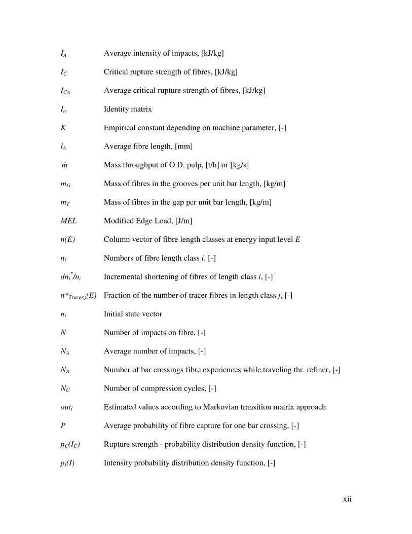
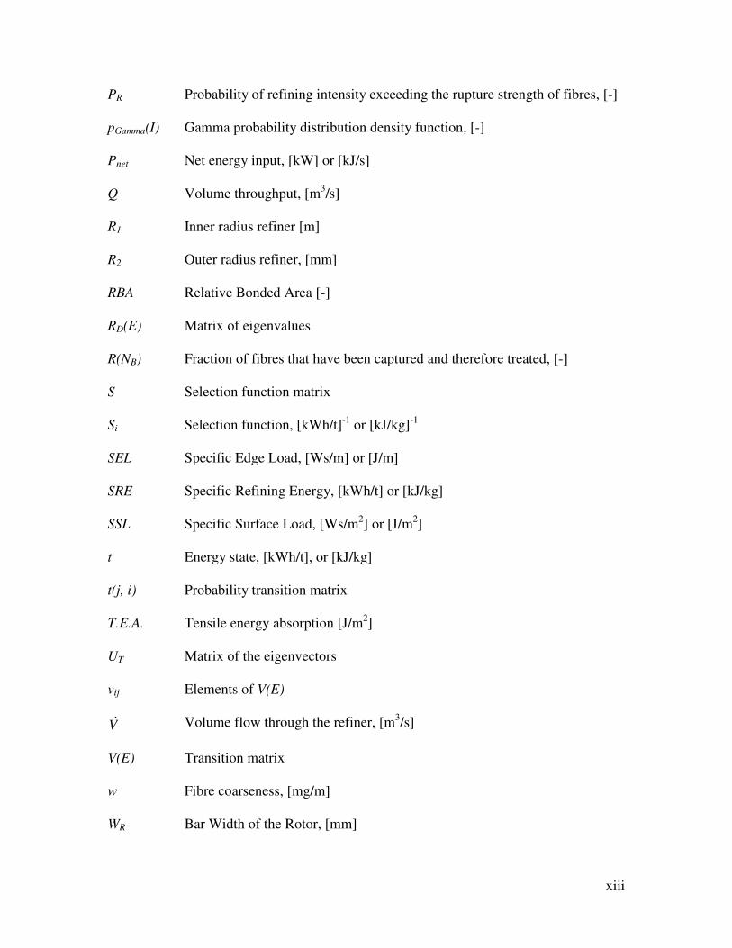
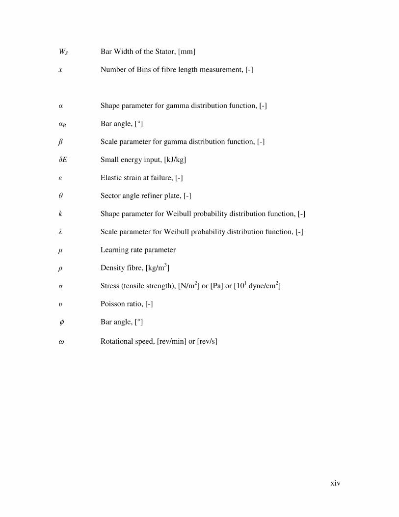