NBER WORKING PAPER SERIES

MEASURED AGGREGATE GAINS FROM INTERNATIONAL TRADE

Ariel BursteinJavier Cravino

Working Paper 17767http://www.nber.org/papers/w17767

NATIONAL BUREAU OF ECONOMIC RESEARCH1050 Massachusetts Avenue

Cambridge, MA 02138January 2012

A previous version of this paper circulated under the title "Trade Liberalizations and Measured RealGDP in Models of International Trade". We thank Costas Arkolakis, Andrew Atkeson, Arnaud Costinot,Robert Feenstra, Jonathan Vogel, and Iván Werning for very useful comments. The views expressedherein are those of the authors and do not necessarily reflect the views of the National Bureau of EconomicResearch.

NBER working papers are circulated for discussion and comment purposes. They have not been peer-reviewed or been subject to the review by the NBER Board of Directors that accompanies officialNBER publications.

© 2012 by Ariel Burstein and Javier Cravino. All rights reserved. Short sections of text, not to exceedtwo paragraphs, may be quoted without explicit permission provided that full credit, including © notice,is given to the source.

Measured Aggregate Gains from International TradeAriel Burstein and Javier CravinoNBER Working Paper No. 17767January 2012JEL No. E01,F1

ABSTRACT

Do theoretical welfare gains from trade translate into aggregate measures of economic activity? Wecalculate the changes in real GDP and real consumption that result from changes in trade costs in arange of workhorse trade models, following the procedures outlined by statistical agencies in the UnitedStates. Our main findings are as follows: First, real GDP and measured aggregate productivity risein response to reductions in variable trade costs if GDP deflators capture the decline in trade costs.Second, with balanced trade in each country, changes in world real consumption and changes in worldreal GDP (i.e.: weighting the change in each country by its nominal GDP) in response to changes invariable trade costs coincide, up to a first-order approximation, with changes in world theoretical (welfare-based)consumption. The equivalence between measured consumption and theoretical consumption holdscountry-by-country under stronger conditions. Third, for given trade shares and changes in variabletrade costs, changes in real GDP and changes in world real consumption are approximately equal inmagnitude across the models we consider.

Ariel BursteinDepartment of EconomicsBunche Hall 8365Box 951477UCLALos Angeles, CA 90095-1477and NBERarielb@econ.ucla.edu

Javier CravinoDepartment of EconomicsUCLABunche Hall 8365Los Angeles, CA 90095-1477jcravino@ucla.edu

1 Introduction

What are the aggregate gains from reductions in the costs of international trade? There are

two major approaches to address this question. A first approach uses structural models to

infer unobservable welfare gains from changes in trade costs or in trade patterns (see e.g.

Eaton and Kortum 2001, Alvarez and Lucas 2007, Arkolakis, Costinot and Rodriguez-Clare

2011, Donaldson 2010, and Waugh 2010). A second approach documents the empirical link

between the level or the change in international trade and aggregate indicators of economic

activity (see e.g. Frankel and Romer 1999, Rodriguez and Rodrik 2001, and Feyrer 2009a,

2009b).

This paper connects these two approaches by studying, within a range of workhorse

models of international trade, the relationship between theoretical welfare gains from trade

and aggregate measures of economic activity, namely real GDP and real consumption as

constructed by national statistical agencies. In doing so, we shed light on the following

questions. Should we expect measured aggregate productivity and real GDP to rise with

trade? Are aggregate measures of economic activity informative of theoretical gains from

trade? Do different models have common sufficient statistics for the impact of trade on

aggregate measures of economic activity?

The models that we base our analysis on include Armington models with perfect competi-

tion and exogenous specialization in production (e.g. Anderson 1979), Ricardian models with

endogenous specialization in production (e.g. Dornbusch, Fisher and Samuelson 1977 and

Eaton and Kortum 2001), and monopolistically competitive firm models with heterogenous

firms and constant markups (e.g. Krugman 1980 and Melitz 2003). We consider extensions

of the model with multiple factors of production (but common factor intensities across pro-

ducers) and with endogenous quality choice. We include international trade costs of the

form of iceberg variable trade costs, fixed export costs (in the model with monopolistic com-

petition), and import tariffs. In all of these models, reductions in international trade costs

typically result in a rise in welfare for the representative consumer.

We calculate these models’ implications of reductions in trade costs for real GDP and real

consumption calculated following the procedures outlined by the Bureau of Labor Analysis

to construct the National Income and Product Accounts (NIPA) in the United States. For

many industries and components of GDP, comprehensive measures of physical quantities

are difficult to obtain in practice. In such cases, real quantities are typically calculated by

deflating current dollar measures of output or consumption with price indices – e.g. in

most cases the producer price index (PPI) for output and the consumer price index (CPI)

for consumption.

We first calculate the change in measured aggregate productivity and real GDP following

a change in international trade costs. We show that, in response to a decline in variable trade

costs, aggregate productivity and real GDP in any country rise only if trade costs are recorded

in GDP and GDP deflators reflect the fall in trade costs. That is, measured productivity

and real GDP rise when variable trade costs fall if the services and activities required to

sell goods abroad (which include shipping services provided by the transportation industry

and, more broadly, any other production, marketing, regulatory, and information costs that

apply differentially to exported products)1 are performed and recorded in the home country,

as opposed to being performed abroad or not measured at all. This is because, under certain

conditions, measured aggregate productivity in any given country only responds to shifts in

its production possibility frontier as is, in principle, desirable for a measure of productivity.2

The response of real GDP also depends on the form of trade liberalization. In particular,

changes in fixed trade costs (if these are expensed and hence not recorded in GDP) have no

direct impact on GDP deflators and hence leave real GDP unchanged. Reductions in import

tariffs increase real GDP from the expenditure side if tariff revenues at constant prices rise

(which requires an increase in the physical quantity of imports).

Next, we compare changes in real GDP and in real consumption (in our baseline model,

changes in consumption expenditures are equal to changes in total absorption). Real GDP

and real consumption can differ even when trade is balanced due to movements in the price

of exports relative to the price of imports (the terms of trade). We show, however, that if

trade is balanced in each country, changes in world real GDP are equal, up to a first-order

approximation, to changes in world real consumption (where each country is weighted by

its current-dollar GDP). The equality holds at the world aggregate level because terms of

trade improvements in one country are associated to terms of trade worsenings in another

country. While changes in real GDP country-by-country depend critically on the patterns

of specialization in the production of trade services, the equality between changes in world

real GDP and world consumption does not.

Perhaps more importantly, we compare changes in measured real consumption with

changes in theoretical (or welfare-based) consumption. Differences between theoretical and

measured consumption arise from differences between consumption deflators and the theo-

retical price index. Consumption deflators in our model differ from the welfare-based price

index in three respects. First, consumption deflators do not fully take into account substitu-

1Anderson and Van Wincoop (2004) argue that these additional costs are at least as important as

narrowly-defined transportation costs.2As shown in Kohli (2004) and Kehoe and Ruhl (2008), the value of production at constant prices does not

respond, to a first-order approximation, to changes in international prices that leave the domestic production

possibility frontier unchanged.

2

tion in consumption from changes in relative prices. Second, they do not take into account

changes in the mass of consumed goods which, in the presence of love for variety, matter

for theoretical consumption. Third, they do not take into account improvements in product

quality if quality changes are measured inaccurately in consumption deflators. The report

by the Boskin Commission (1996) examines in detail how these and other biases in the CPI

lead to an understatement of real consumption growth in the U.S.

We show how, under certain conditions, these multiple biases in consumption deflators

may not result in a mismeasurement of theoretical consumption. If the set of consumed goods

and product quality are fixed (so that the second and third sources of the bias are absent),

then in response to any type of trade cost movement, changes in theoretical consumption

are bounded between measured real consumption calculated using initial base-year prices

and real consumption using end base-year prices. This implies, as is well-known (see e.g.

Hausman 2003), that the substitution bias is of second order: in each country, changes in real

consumption equal changes in theoretical consumption, up to a first-order approximation.

When the set of consumed goods and product quality are not fixed, we establish the

following result. In response to changes in variable trade costs, with trade balance in each

country, changes in world real consumption equal changes in world theoretical consumption

(defined analogously to world real consumption and world real GDP), up to a first-order

approximation. That is, while changes in theoretical consumption and real consumption

may differ country-by-country, these differences cancel-out when adding them across coun-

tries in the world. Under stronger assumptions (i.e. Pareto distribution of entering firms’

productivity and fixed export costs paid in the destination market, as in Eaton, Kortum, and

Kramarz 2010), the equality between measured consumption and theoretical consumption

holds country-by-country, up to a first-order approximation, as in the model with a fixed set

of consumed goods. We also show that, in response to large reductions in variable trade costs

(for which we must solve the model numerically), the elasticities of theoretical consumption

and real consumption can be quite close, country-by-country (and hence also at the world

level), independently of whether fixed export costs are incurred domestically or abroad.

Finally, we ask whether the different models that we consider give rise to different suf-

ficient statistics for measured gains from trade. We consider this question separately for

our measures of real GDP and real consumption. Across our range of models, we obtain a

common expression for the change in real GDP as an average of changes in variable trade

costs weighted by export shares of continuing exporting producers. Conditional on this di-

rect impact of changes in trade costs, reallocation of production from less productive to more

productive producers, entry and exit into production and exporting, and changes in the mass

of producers, have no additional effects on changes in measured aggregate productivity and

3

real GDP.

We also show that across our range of models, changes in world real consumption and

world real GDP are equal in magnitude, up to a first-order approximation, for given trade

shares and for given changes in variable trade costs. This first-order equivalence in mea-

sured gains from trade in consumption across seemingly different models does not reflect

an inadequacy of the aggregate measures of real consumption. Instead, this equivalence in

measured gains from trade is consistent with the underlying equivalence in the welfare im-

plications of these models under some restrictions, as demonstrated by Arkolakis, Costinot

and Rodriguez-Clare (2011) and Atkeson and Burstein (2010). Note, however, that changes

in fixed trade costs or foreign country size that increase trade shares (and also welfare, un-

der the assumptions of Arkolakis, Costinot and Rodriguez-Clare 2011) may not result in

measured gains from trade.

Our paper is related to a recent paper by Bajona, Gibson, Kehoe, and Ruhl (2010),

who ask whether the increase in welfare following a trade liberalization translates into an

increase in real GDP as measured in NIPA. They conclude, as summarized in Kehoe and

Ruhl (2010), that “...standard trade models do not imply that opening to trade increases

productivity or real GDP, but that it increases welfare”. The two main differences of our

paper relative to Bajona et. al. (2010) are as follows. First, while Bajona et. al. (2010)

focus on the implications of trade liberalization on real GDP, we also study the effects on

real consumption and provide conditions under which the response of real consumption to

changes in trade costs equals that of theoretical consumption. Second, Bajona et. al. (2010)

focus on cases in which price indices do not directly reflect changes in international trade

costs, either because trade costs are fully incurred abroad or because countries are in autarky

before the trade liberalization (in which case price indices of exported goods, as measured by

the BLS, are not well defined since there are no continuing exported goods). In the class of

models considered in both papers, this implies that measured real GDP is unchanged with

trade liberalization (abstracting from changes in real tariff revenues). We show, however,

that starting with positive trade levels, any reduction in trade costs that is reflected in price

indices does result in an increase in real GDP.

Our work is also related to Feenstra (1994) and Broda andWeinstein (2006), who quantify

the mismeasured growth in real consumption in the U.S due to the rise in the number of

imported varieties that is not accounted for in the CPI, without taking a stand on the

source of the growth in the number of imported varieties.3 We show in our models that, in

3Relatedly, Feenstra, Reinsdorf, and Slaughter (2008) and Neiman and Gopinath (2011) argue that if

export and import price indices are mismeasured (among other reasons, due to changes in import variety),

changes in tariffs or in the terms of trade can result in changes in measured aggregate productivity.

4

response to a reduction in variable trade costs that results in a rise in the number of imported

varieties, to a first-order approximation there is no bias in consumption deflators at the

world aggregate level or, under stronger conditions, country-by-country, when simultaneously

taking into account in general equilibrium other biases in the price indices. Hence, any

underestimate of real consumption growth stemming from an increase in the mass of imported

varieties that is not captured in the import price index is offset by the other biases in the

CPI. Finally, our paper is related to the work of Pavcnik (2002) and others, that construct

measures of aggregate productivity as weighted averages of productivity estimates across

producers. While those measures of aggregate productivity may reflect the reallocation of

production towards more productive producers induced by trade liberalization, we argue,

using a range of models of trade and firm heterogeneity as a laboratory, that measures of

aggregate productivity constructed from NIPA do not capture this reallocation.

The paper is organized as follows. Section 2 presents an overview of the measurement

procedures that we use in our models. Section 3 presents our baseline Armington model with

exogenous specialization in the set of goods that are produced and traded in each country.

Section 4 derives our basic results on measured real GDP, real consumption, and theoretical

consumption in the Armington model. Section 5 shows that these basic results apply in a

Ricardian model with endogenous specialization and perfect competition. Section 6 extends

the basic results to the version of the model with endogenous specialization and monopolistic

competition. Section 7 considers two additional extensions: endogenous quality choice and

multiple factors of production. Section 8 concludes. Various proofs and details are relegated

to the Appendix.

2 Aggregate Measurement: Overview

In this section we provide a brief overview of the procedures that we use to calculate changes

in aggregate quantities. We follow as closely as possible the procedures outlined by the

Bureau of Economic Analysis in the United States to construct the National Income and

Product Accounts (NIPA).4

To calculate aggregate measures of output such as real GDP, or aggregate measures of

expenditures such as real consumption, we use a Fisher index, which is a geometric average

of a Laspeyres and a Paasche quantity index. For example, real GDP in period relative to

4See, e.g. Concepts and Methods of the U.S. National Income and Product Accounts (2009). The

procedures that we consider are broadly consistent with the recommendations by the United Nations in

their System of National Accounts.

5

period − 1 is given by

−1=

µ P−1P−1−1

¶05×µ P

P−1

¶05 (1)

where and denote prices and quantities in period of the detailed components of GDP,

and where the sum is calculated across all of these components. The terms −1 and −1represent "real" quantities of any given GDP component evaluated at constant prices. The

first term in expression (1) is a Laspeyres quantity index (based on − 1 prices), while thesecond term is a Paasche quantity index (based on prices).5 Real GDP in period relative

to period 0 is given by

0=

Y=1

−1. (2)

The detailed components of GDP in expression (1) can be industries, sectors, or groups

of narrowly defined goods that jointly conform aggregate GDP or other aggregate measures

of output and expenditures. While estimates of the current-dollar value of production, ,

are typically available for each of these individual components, data on physical quantities,

, are often not.

For those components of GDP for which data on physical output are available, real quan-

tities are computed using either the direct valuation method (sum of quantities evaluated at

constant prices) or the quantity extrapolation method (using a quantity indicator that ap-

proximates the movements of the component series). For those components of GDP for which

estimates of physical quantities are not available, real quantities are estimated using the de-

flation method, dividing current-dollar values by appropriate price indices.6 In particular,

for any component of GDP, −1 = () (PP−1) and −1 = (−1−1)× (PP−1)

where PP−1 denotes the change in the price index between periods − 1 and . In our

baseline calculations, we compute aggregate quantities using the deflation method.

To calculate real GDP from the production side using the deflation method, we deflate

the current-dollar value added of production (including the value added of the activities

performed at home to sell goods internationally) using the producer price index (PPI) as a

5The implicit GDP deflator is calculated as the ratio of current-dollar GDP to real GDP,

(P

P

−1−1) (−1), which is equal to a geometric average of a Laspeyres and aPaasche price index.

6The direct valuation method is used, for example, to calculate real output of autos and light trucks,

while quantity extrapolation is used to calculate real output of housing and utilities services. The majority

of the other subcomponents of GDP are calculated using the deflation method since physical output is not

recorded across producers (see "Summary of NIPA Methodologies", p.12 for a description of the method

used to estimate each subcomponent of GDP).

6

deflator.7 The change in the PPI between periods − 1 and is a weighted average of price

changes between these two periods across goods and services that are produced domestically

to sell at home or to export abroad.8

We consider two alternative deflation procedures. The first procedure deflates the total

value of production using a single aggregate price index. The second procedure deflates

the value of output bound for each destination using a destination-specific price index. We

show that, using disaggregated deflators by destination country, real GDP is equal to that

obtained using the direct valuation method based on data on physical quantities of each

commodity.

Export prices in the PPI and in the export price index (EPI) are typically measured

at fob (i.e. free-on-board) values, and hence exclude shipping services incurred abroad. A

critical assumption determining the impact of changes in international trade costs on mea-

sured real GDP is whether changes in measured prices in the PPI reflect, at least partly,

these changes in trade costs. In addition to shipping costs (that are included in the trans-

portation industry), international trade costs include production and marketing costs that

apply differentially to exported goods, information costs, costs associated with the use of

different currencies, contract enforcement costs, legal regulatory costs, and other time costs

associated to international trade (see e.g. Anderson and Van Wincoop 2004). To understand

the implications of the nature of trade costs on aggregate measurement, we consider two al-

ternative specifications. In our baseline specification, we assume that the activities required

to sell goods abroad are performed in the home country, and hence changes in the variable

component of these trade costs are reflected in the home PPI. In an alternative specification,

we assume that all export costs are incurred in foreign countries, in which case changes in

trade costs are not reflected in the PPI.

We also calculate GDP from the expenditure side, defined as current-dollar absorption

(which in our baseline model is equal to consumption), plus exports less imports. Real

consumption is calculated analogously to real GDP (using expressions 1 and 2), but deflating

7This is the procedure used in the GDP by industry accounts published by the BEA. When intermediate

inputs are used in production, real value added is calculated using the double deflation method. This consists

of first deflating gross output and inputs separately (using their respective PPIs), and then computing real

value added as the difference between real gross output and real intermediate inputs.8To construct the PPI, the Bureau of Labor Statistics (BLS) collects prices for a sample of items that

can be priced consistently through time. Price indices are then constructed by averaging price changes of

individual items weighted by the the value of production in some base year. The set of sampled items and

the weights are updated every few years (between 5 and 7 years for the typical good in the PPI). Price

changes from product replacements tend to be dropped from the index, which is equivalent to attributing

to discontinued goods the rate of change in the overall price index. For more details on the construction of

producer price indices and international price indices in the US, see Chapters 14 and 15 of the BLS Handbook

of Methods.

7

each component of nominal consumption (when physical quantities are not available) by its

consumer price index (CPI) instead of the PPI. The change in the CPI is a weighted average

of consumer price changes of domestic and imported goods consumed in both time periods.9

In the presence of import tariffs, current-dollar GDP from the expenditure side (defined

as the sum of final expenditures including tariffs) is not equal to current-dollar GDP from

the production side (defined as the sum of firm value added excluding tariffs). In order to

reconcile estimates of GDP from the production and expenditure sides, the BEA adds import

taxes to factor payments when computing value added by industry.10 To be consistent with

this procedure, in the model with tariffs we calculate real GDP from the expenditure side. In

deflating consumption expenditures, the CPI is constructed using prices inclusive of tariffs.

In deflating imports, the import price index (IPI) is constructed using prices exclusive of

import tariffs.

3 Model with Exogenous Specialization and Perfect Competition

In this section we present an Armington version of our model with exogenous specialization

and perfect competition. The extensions of the model that follow build upon this basic

setup.

The world economy is composed of countries. The utility of the representative consumer

in country is

=

∞X=0

() , ≤ 1

where denotes theoretical consumption of the final good at time , given by

=

∙ZΩ

()−1 d

¸ −1. (3)

Here, () denotes the consumption of good and Ω denotes the set of available differ-

entiated goods in country . The parameter denotes the elasticity of substitution across

9See "Updated Summary of NIPA Methodologies", for details on the deflator used in each expenditure

component of GDP. See McCully, Moyer, and Stewart (2007) for a detailed comparison of the CPI and the

implicit deflator for personal consumption (where the latter is constructed as the ratio of nominal and real

consumption). See Feenstra, Heston, Timmer, and Deng (2009) for a detailed discussion of the relation

between real GDP from the production side and real GDP from the expenditure side as measured in the

Penn World Tables.10In particular, in the "Gross Domestic Product by Industry Accounts" computed by the BEA, value added

is defined as the sum of: "Compensation of employees", "Taxes on production and imports less subsidies"

and "Gross operating surplus". For a detailed description of the transactions that are included in value

added, see "Concepts and Methods of the U.C. Input-Output Accounts", Chapter 6, under "Value-added

transactions".

8

varieties. In the model with monopolistic competition below we assume 1. Demand

for each good is () = [

() ]

−, where () denotes the consumer price of

good in country and =hR

Ω ()

1−di 11−

is the welfare-based price index in

country . We assume that consumption of the final good and the welfare-based price

index cannot be directly observable (or similarly, that the final good is not a physically

traded commodity). If and were directly observable, then measuring the gains from

trade would be straightforward.

Each producer specializes in the production of a single differentiated good. Production

uses labor according to the production function = , where and denote output and labor

of a producer with productivity (multiple inputs are introduced in Section 7). We denote

by () the distribution of producers, indicating the mass of producers with productivity

in country at time . Given the symmetry of goods in the production function of the final

good (3), we interchangeably index goods by , or by their productivity and source country

. For example, () and () denote the consumption quantity and price, respectively,

in country of good produced by producers in country . We assume that all prices are

already expressed in a common currency (which we refer to as dollars).

Goods can be internationally traded subject to a technology described below. We denote

by Ω the set of producers (indexed by their productivity) from country that sell a positive

quantity to country at time . In the absence of international trade between countries

and at time , the set Ω is empty.

In the model with exogenous specialization, we assume that the distribution of producers,

(), is exogenously given and constant over time. We also assume that the set of goods

that are internationally traded, Ω, is exogenously given and that, as long as there is any

trade between countries and , it is constant over time. We do not make assumptions on

how the set of goods Ω varies across destinations, hence not all goods sold domestically

need to be exported, and vice-versa. For example, only goods with high productivity might

be traded. The case of Ω = Ω corresponds to the Armington model in which all goods

are internationally traded (unless countries are in autarky).

Goods can be shipped across countries subject to iceberg variable international trade

costs. In our baseline specification, we assume that international trade costs are incurred in

each source country, as is typically assumed in the literature.11 In particular, each unit of

a good produced in country with productivity shipped to country at time requires

( − 1) units of labor from country , where ≥ 1 and = 1. International

11While in this formulation we assume that trade costs use factors of production in the exporting country,

we can instead assume that they use factors from the importing country (or from both). This would

complicate the notation without changing substantially the results.

9

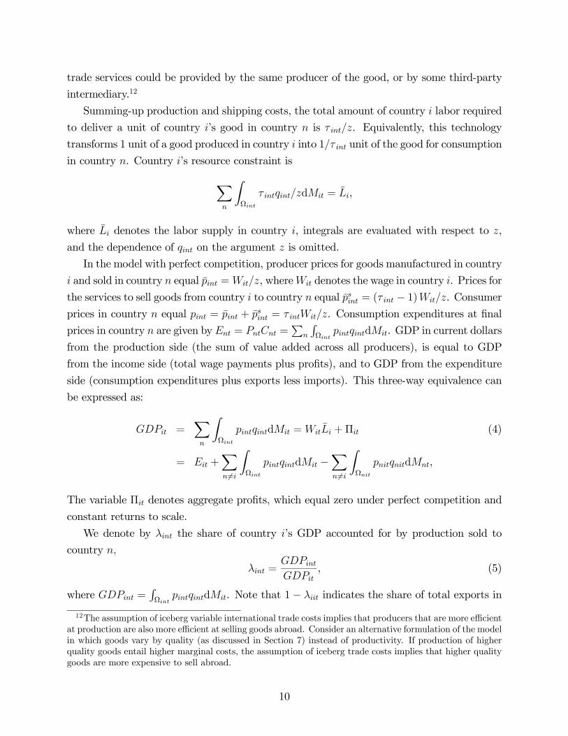
trade services could be provided by the same producer of the good, or by some third-party

intermediary.12

Summing-up production and shipping costs, the total amount of country labor required

to deliver a unit of country ’s good in country is . Equivalently, this technology

transforms 1 unit of a good produced in country into 1 unit of the good for consumption

in country . Country ’s resource constraint is

X

ZΩ

d = ,

where denotes the labor supply in country , integrals are evaluated with respect to ,

and the dependence of on the argument is omitted.

In the model with perfect competition, producer prices for goods manufactured in country

and sold in country equal =, where denotes the wage in country . Prices for

the services to sell goods from country to country equal = ( − 1). Consumer

prices in country equal = + = . Consumption expenditures at final

prices in country are given by = =P

RΩ

d. GDP in current dollars

from the production side (the sum of value added across all producers), is equal to GDP

from the income side (total wage payments plus profits), and to GDP from the expenditure

side (consumption expenditures plus exports less imports). This three-way equivalence can

be expressed as:

=X

ZΩ

d = +Π (4)

= +X6=

ZΩ

d −X6=

ZΩ

d,

The variable Π denotes aggregate profits, which equal zero under perfect competition and

constant returns to scale.

We denote by the share of country ’s GDP accounted for by production sold to

country

=

, (5)

where =RΩ

d. Note that 1− indicates the share of total exports in

12The assumption of iceberg variable international trade costs implies that producers that are more efficient

at production are also more efficient at selling goods abroad. Consider an alternative formulation of the model

in which goods vary by quality (as discussed in Section 7) instead of productivity. If production of higher

quality goods entail higher marginal costs, the assumption of iceberg trade costs implies that higher quality

goods are more expensive to sell abroad.

10

country ’s GDP.

4 Results: Exogenous Specialization and Perfect Competition

In this section, we present our results in the basic model with exogenous specialization and

perfect competition. We first calculate changes in real GDP in response to changes in variable

trade costs. We then show how changes in real GDP vary if we assume that the production

of international trade services is specialized in one country. We then compare changes in real

consumption and theoretical consumption, and next compare changes in world real GDP and

world real consumption. Finally, we calculate the response of real GDP and consumption to

changes in tariffs. We conclude this section by summarizing the results.

Real GDP

We first construct real GDP from the production side. In order to apply expressions (1) and

(2), we must specify how goods are grouped into components of GDP. We consider two cases.

First, we aggregate production by all producers to all destinations into a single component,

and construct real quantities by deflating current-dollar GDP using a single, aggregate de-

flator. Second, we decompose total production by destination country, and calculate real

quantities by deflating destination-specific production values using destination-specific price

indices.13 We show that real GDP under the second case is equal to real GDP constructed

using the direct valuation method in which data on physical quantities and prices of indi-

vidual producers (i.e. , ) is used.

Real GDP using aggregate deflators: We construct real quantities by deflating the total

current-dollar value of production with the aggregate PPI. The PPI is a weighted average

of changes in producer prices of continuing goods, based on production weights in period 0.

We do not make assumptions on what the base-year 0 is or how frequently it is updated

with the exit of existing products or the entry of new products. The PPI in country in

13In both cases, in defining these detailed components of GDP, we are implicitly assuming that in the model

there is a representative sector or industry composed of differentiated goods which aggregate according to

(3). Extending the model to allow for heterogeneous industries or sectors, aggregated into the final good

with an outer CES technology, is straighforward at the expense of extra notation, and does not substantially

alter our results.

11

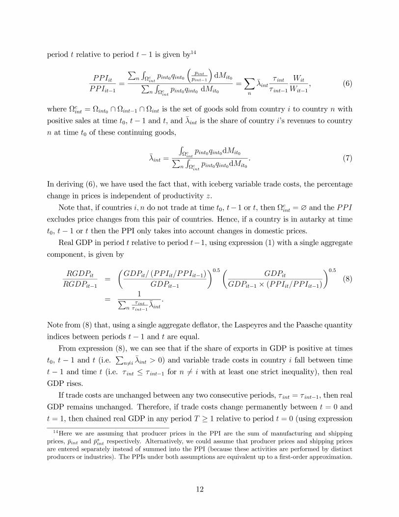
period relative to period − 1 is given by14

−1=

P

RΩ

00

³

−1

´d0P

RΩ

00 d0

=X

−1

−1, (6)

where Ω = Ω0 ∩ Ω−1 ∩ Ω is the set of goods sold from country to country with

positive sales at time 0, − 1 and , and is the share of country ’s revenues to country

at time 0 of these continuing goods,

=

RΩ

00d0P

RΩ

00d0

. (7)

In deriving (6), we have used the fact that, with iceberg variable trade costs, the percentage

change in prices is independent of productivity .

Note that, if countries do not trade at time 0, −1 or , then Ω = ∅ and the

excludes price changes from this pair of countries. Hence, if a country is in autarky at time

0, − 1 or then the PPI only takes into account changes in domestic prices.Real GDP in period relative to period −1, using expression (1) with a single aggregate

component, is given by

−1=

µ (−1)

−1

¶05µ

−1 × (−1)¶05

(8)

=1P

−1

.

Note from (8) that, using a single aggregate deflator, the Laspeyres and the Paasche quantity

indices between periods − 1 and are equal.

From expression (8), we can see that if the share of exports in GDP is positive at times

0, − 1 and (i.e.P

6= 0) and variable trade costs in country fall between time

− 1 and time (i.e. ≤ −1 for 6= with at least one strict inequality), then real

GDP rises.

If trade costs are unchanged between any two consecutive periods, = −1, then real

GDP remains unchanged. Therefore, if trade costs change permanently between = 0 and

= 1, then chained real GDP in any period ≥ 1 relative to period = 0 (using expression14Here we are assuming that producer prices in the PPI are the sum of manufacturing and shipping

prices, and respectively. Alternatively, we could assume that producer prices and shipping prices

are entered separately instead of summed into the PPI (because these activities are performed by distinct

producers or industries). The PPIs under both assumptions are equivalent up to a first-order approximation.

12

2) is given by

0

=1

0

. (9)

Intuitively, a reduction in variable trade costs entails an improvement of domestic tech-

nologies, which lowers producer prices relative to the wage, and increases real GDP. This rise

in real GDP shows up as a rise in aggregate productivity. If the PPI does not take into ac-

count changes in trade costs (or if a country is initially in autarky), then =0 ,

and −1 = 1.

Note that any reallocation in production towards more productive producers (due to,

for example, a higher productivity of exporters relative to non-exporters) does not result in

larger changes in measured aggregate productivity. To understand this implication of the

model, we can rewrite the ratio of real GDP in period to relative to period − 1, using (4)and (8) as

−1=

P

RΩ

×

dP

RΩ−1

−1−1

× −1−1−1

d−1

−1

1

−1, (10)

where () denotes production labor used by country producers with productivity

to sell in country , and denotes the aggregate quantity of labor used for production

in country (equal to in this model). Note that value added per worker by individual

producers, () () (), is equal to the wage, , for all producers independent of

their productivity . UsingP

RΩ

d = 1 and (6) we obtain expression (8). Therefore,

any reallocation of labor towards more productive producers does not result in any further

increase of aggregate productivity beyond the direct effect from a reduction in variable trade

costs.15

Real GDP using disaggregated deflators: We now compute real quantities by deflating

destination-specific production values using destination-specific PPIs. The PPI in period

relative to period − 1 for goods produced in country and shipped to country is

−1=

RΩ

00

³

−1

´d0R

Ω00d0

=

−1

−1. (11)

Here we used the fact that percentage changes in producer prices are equal for all goods

bound to a given destination. The disaggregated deflator −1 is well defined

only when the set of continuing goods is non-empty.

15Note that if the PPI were calculated as a change in average prices (instead of an average change in

prices), then reallocation of production towards more productive producers would result in a larger decline

in the PPI and a higher increase in real GDP.

13

Real GDP in period relative to period −1, using equation (1) with destination-specificGDP components, is given by

−1=

ÃP

−1P−1

!05µ PP

−1 × −1

¶05(12)

=

à P

−1 P

−1

−1

!05.

Note that, in contrast to the measures of real GDP based on aggregate deflators, the

Laspeyres and the Paasche quantity indices of real GDP are not equal when we use dis-

aggregated deflators. From expression (12), if trade costs fall between time − 1 and , thenreal GDP rises. If trade costs change permanently between = 0 and = 1, then chained

real GDP in any period ≥ 1 relative to period = 0 is equal to 10, as in

expression (9).

The expressions for changes in real GDP based on aggregated and disaggregated deflators,

given by (8) and (12), differ in terms of the base-year in which trade shares are calculated.

However, up to a first-order approximation (i.e. around −1 ' 1), the two measuresof changes in real GDP are equal and given by

log = log −X

log = −X

log . (13)

Note that we can re-write the change in real GDP based on disaggregated deflators in

the first line of expression (12) as

−1=

à P

RΩ

−1dP

RΩ−1

−1−1d−1

!05Ã P

RΩ

dP

RΩ−1

−1d−1

!05.

Here we used the fact that the term (−1) in (12) is equal toP

RΩ

−1d, and the term −1 × −1 is equal toP

RΩ−1

−1d−1. This expression corresponds to the change in real GDP cal-

culated according to the direct valuation method (a geometric average of Laspeyres and

Paasche quantity indices), evaluating using production values at constant prices. While this

procedure requires data on physical quantities and prices of individual commodities (which

is typically not available in many industries and subset of goods), what we showed is that

the implied change in real GDP is equal to that using the deflation method with country

specific price deflators.

14

Real GDP under international specialization of shipping services

We now consider an alternative specification on the nature of trade costs in which a subset of

countries specializes in producing shipping services for all other countries. For concreteness

(but without loss of generality for our results), we assume that the world-wide production

of shipping services is concentrated in country . That is, shipping one unit of a good

produced in country with productivity to country at time , for all countries and

, requires ( − 1) units of country ’s labor. Prices received by producers of these

services in country for the services to sell goods from country to country equal =

( − 1), and consumer prices in country equal = ( + ( − 1)) .

The resource constraint in country is

X

ZΩ

d = for 6= ,

while in country it isX

ZΩ

d +X6=

X

ZΩ

( − 1) d =

GDP in current dollars from the production side in country 6= is =P

RΩ

d,

while in country = it is

=X

ZΩ

¡ +

¢d +

X6=

X

ZΩ

d

In countries 6= that do not specialize in shipping services, the PPI is simply

−1 = −1, and the ratio of real GDP in periods and − 1 is−1 = 1.

In contrast to the previous specification, changes in trade costs now leave domestic tech-

nologies unchanged for those countries that do not specialize in shipping services. Hence, in

these countries changes in the PPI are equal to changes in the wage, so real GDP remains

unchanged. This result holds more generally, if changes in foreign trade costs also change

relative prices faced by different domestic producers (as in the Hecksher-Ohlin model, for

example) but not their technologies. To see this, recall that when calculating real quantities

by deflating the value of production with destination specific PPIs, real GDP is equal to the

value of production evaluated at constant-year prices. From revealed production choices, the

value of production falls (rises) between − 1 and when evaluated at − 1 () prices. To afirst-order approximation, real GDP remains constant. This line-of-argument cannot be used

15

when changes in trade costs change domestic technologies, as in our baseline specification.

In Appendix B we derive the change in real GDP in country that specializes in the

production of shipping services. Reductions in trade costs (across any pair of countries) do

improve domestic technologies in country . Hence, in response to any reduction in trade

costs, the PPI falls relative to the wage, and real GDP rises.

Measured real consumption and theoretical consumption in each country

We now calculate changes in real consumption, and compare them to changes in theoretical

(or welfare-based) consumption of individual countries. As we did for real GDP, we use the

deflation method, first using an aggregate deflator and then using country-specific deflators.

Real consumption using aggregate deflators: We calculate real consumption using the defla-

tion method, deflating consumption expenditures with a consumer price index (CPI). We

construct the CPI as a weighted average of ratios of final prices between two periods (of

goods that are consumed in both periods) using 0 weights. The CPI in country at time

relative to time − 1 is given by

−1=

P

RΩ

¡0

0

¢ ³

−1

´d0P

RΩ

0

0d0

. (14)

Real consumption in country at time relative to − 1, using expression (1) with asingle aggregate component, is given by

−1=

µ (−1)

−1

¶05µ

−1 × (−1)¶05

(15)

= (−1)

−1.

The ratio of theoretical consumption in periods and − 1 is equal to −1 =

(−1)(−1), where is the welfare-based price index defined above. Hence,

differences between changes in real consumption and theoretical consumption stem only from

differences between the CPI and the theoretical CES price index. It is straightforward to

show that, to a first-order approximation, the log change in the CES price index with a fixed

set of goods is equal to an expenditure-weighted average of log price changes of individual

goods, as it is for the CPI defined in expression (14). Hence, for marginal changes in prices,

changes in real consumption coincide with changes in theoretical consumption, country-by-

country.

16

Large changes in prices give rise to the well-known substitution bias. However, if the

CPI is evaluated using 0 = − 1 or 0 = weights, we can bound this substitution bias.

In particular, in Appendix A we show that, if the set of goods consumed in each period is

unchanged, then the CPI with initial (final) period weights, 0 = − 1 (0 = ) overstates

(understates) changes in the welfare-based price index between periods − 1 and . That is,

−1

¯0=

≤

−1≤

−1

¯0=−1

. (16)

Hence, changes in theoretical consumption are bounded above (below) by real-consumption

calculated with the CPI based on final (initial) period weights.16 These results hold under

both specifications of international trade costs.

Real consumption using disaggregated deflators: We now calculate changes in real con-

sumption by deflating source—country specific consumption expenditures using their respec-

tive CPIs. Country specific expenditures and CPIs are defined, respectively, as =RΩ

d and

−1=

RΩ

0

0

³

−1

´d0R

Ω0

0d0

.

Real consumption in period relative to period − 1, using equation (1) with country-specific expenditure components, is given by

−1=

ÃP

−1P

−1

!05µ PP

−1 × −1

¶05(17)

=

à P

RΩ

−1dP

RΩ−1

−1−1d−1

!05Ã P

RΩ

dP

RΩ−1

−1d−1

!05,

where we used the fact that percentage changes in all prices for goods coming from a common

source country are equal. This expression coincides with a geometric average of Laspeyres

and Paasche quantity indices using the direct-valuation method.

Up to a first-order approximation, changes in real consumption based on aggregate de-

flators and disaggregated deflators (as well as theoretical consumption) are equal and given

16Inequality (16) does not hold in the case in which there is no trade between countries and at time

− 1 or , so that Ω = ∅ In this case, inequality (16) would hold if the CPI to incorporated price changesfor all goods, including those that are not consumed, and assumed that unavailable goods have an infinite

price. However, this is not the approach taken by the national statistics when calculating the CPI.

17

by

log = log −X

log. (18)

World real GDP, consumption, and theoretical consumption

As can be observed by comparing expressions (13) and (18), differences between changes in

real GDP and real consumption, country-by-country, arise from (1) differences between the

current-dollar value of consumption and GDP (in the presence of trade imbalances) and (2)

differences between changes in the PPI and in the CPI due to movements in relative wages

and relative trade costs that change the price of exports relative to imports (i.e. the terms

of trade) in each country.

We now show that, if trade is balanced in each country, a weighted-average (based on

each country’s current-dollar GDP) of changes in real consumption across countries is equal

to the same weighted average of changes in real GDP across countries, up to a first-order

approximation. Here we consider the baseline specification of trade costs in which these

are incurred using labor in each exporting country. In the Appendix we show that the

equivalence between changes in world real GDP and world real consumption also holds in

the model in which a subset of countries specializes in the production of shipping services.

Define to be country ’s share in total current-dollar GDP across all countries in period

: = P

. From expression (13), the world change in real GDP is, to a

first-order approximation,

X

log =1P

"X

log −X

X

log

#.

(19)

From expression (18), assuming balanced trade in each country (so that, as can be seen in

4, GDP and expenditures in current-dollars are equal, = ), the world change in

real consumption is, to a first-order approximation,

X

log =1P

"X

log −X

X

log

#. (20)

The first term in expression (19) is equal to the first term in expression (20) because

log = log. The second term in expression (19) is equal to the second term

in expression (20) because log = log. Intuitively, for any pair

of trading countries, an improvement in the bilateral terms of trade for one country implies

a worsening in the terms of trade for the other country. Hence, changes in the world CPI

are equal to changes in the world PPI, and so are world real consumption and world real

18

GDP.17

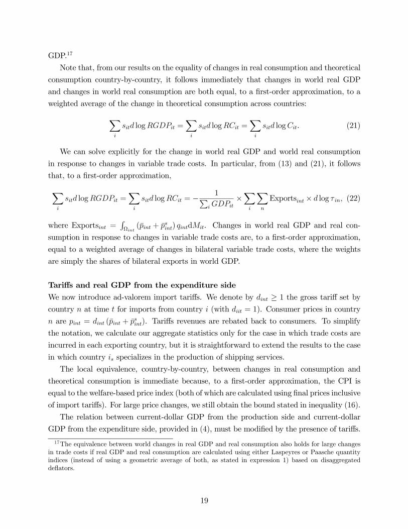
Note that, from our results on the equality of changes in real consumption and theoretical

consumption country-by-country, it follows immediately that changes in world real GDP

and changes in world real consumption are both equal, to a first-order approximation, to a

weighted average of the change in theoretical consumption across countries:X

log =X

log =X

log. (21)

We can solve explicitly for the change in world real GDP and world real consumption

in response to changes in variable trade costs. In particular, from (13) and (21), it follows

that, to a first-order approximation,

X

log =X

log = − 1P

×X

X

Exports× log (22)

where Exports =RΩ

( + ) d. Changes in world real GDP and real con-

sumption in response to changes in variable trade costs are, to a first-order approximation,

equal to a weighted average of changes in bilateral variable trade costs, where the weights

are simply the shares of bilateral exports in world GDP.

Tariffs and real GDP from the expenditure side

We now introduce ad-valorem import tariffs. We denote by ≥ 1 the gross tariff set bycountry at time for imports from country (with = 1). Consumer prices in country

are = ( + ). Tariffs revenues are rebated back to consumers. To simplify

the notation, we calculate our aggregate statistics only for the case in which trade costs are

incurred in each exporting country, but it is straightforward to extend the results to the case

in which country specializes in the production of shipping services.

The local equivalence, country-by-country, between changes in real consumption and

theoretical consumption is immediate because, to a first-order approximation, the CPI is

equal to the welfare-based price index (both of which are calculated using final prices inclusive

of import tariffs). For large price changes, we still obtain the bound stated in inequality (16).

The relation between current-dollar GDP from the production side and current-dollar

GDP from the expenditure side, provided in (4), must be modified by the presence of tariffs.

17The equivalence between world changes in real GDP and real consumption also holds for large changes

in trade costs if real GDP and real consumption are calculated using either Laspeyres or Paasche quantity

indices (instead of using a geometric average of both, as stated in expression 1) based on disaggregated

deflators.

19

For example, in country 6= , we have

=X

ZΩ

( + ) d +Υ = +Π +Υ (23)

= +X6=

ZΩ

( + ) d −X6=

ZΩ

( + ) d,

whereΥ =P

( − 1)RΩ

( + ) denotes tariff revenues collected in coun-

try .

Real GDP calculated from the production side excluding import tariffs from both current-

dollar GDP and from price deflators is unchanged to changes in tariffs for the same reasons

that real GDP in the model with only trade costs is unchanged to changes in trade costs if

these are excluded from price indices.

We now calculate real GDP from the expenditure side by separately deflating each

country-specific expenditure component of GDP. The export price index (EPI) for goods

sold by country to country is given by

−1=

RΩ

¡0 + 0

¢0

³+

−1+−1

´d0R

Ω

¡0 + 0

¢0d0

. (24)

The imports price index (IPI) in country for goods imported from country (inclu-

sive of trade costs incurred abroad but exclusive of tariffs) is given by −1 =

−1.

The Laspeyres real GDP index in country is given by

−1=

P

−1

+P

6=h

Exports−1

− Exports−1

i−1

= (25)

=

P

RΩ

¡−1 + −1

¢d +

P

RΩ

(−1 − 1)¡−1 + −1

¢dP

RΩ−1

¡−1 + −1

¢−1d−1 +

P

RΩ−1

(−1 − 1)¡−1 + −1

¢−1d−1

.

The first term in expression (25) indicates the change in the constant-price value of pro-

duction, and the second term represents the change in the constant price value of tariffs.

The Paasche real GDP index is calculated analogously to the Laspeyres real GDP index,

but using constant period prices and tariffs instead of period − 1 prices and tariffs. Thechange in real GDP between period − 1 and is a geometric average of the Laspeyres and

Paasche indices, as defined in expression (1).

20

Note that, in the absence of tariffs, real GDP from the expenditure side coincides with real

GDP from the production side using disaggregated deflators.18 In the presence of tariffs, there

is an additional source of changes in real GDP. Specifically, real GDP rises if the value of tariff

revenues evaluated at base-prices and base-tariffs,P

6=RΩ

(0 − 1)¡0 + 0

¢d

(with 0 = − 1 or 0 = ), increases. That is, real GDP rises if imported physical quantities

weakly increase.

Finally, consider the equivalence between world real consumption and world real GDP.

Suppose that each country is under balanced trade (exclusive of tariffs),

i.e.P

RΩ

( + ) d =P

RΩ

( + ) d. In this case, from (23),

current-dollar GDP (inclusive of import-tariffs) is equal to current-dollar expenditures. De-

fine country-specific weights based on current-dollar GDP (inclusive of import-tariffs), =

P

. It is straightforward to show, following the steps above in the model

without tariffs, that the change in world real GDP is equal, to a first-order approximation,

to the world change in real consumption, as indicated in expression (21).

Summary of Results

Our central results on the implications of changes in trade costs on measures of real GDP

and real consumption in our model with exogenous specialization and perfect competition

can be summarized as follows:

Result 1: In response to reductions in variable international trade costs incurred in

country that are captured in GDP and its deflators, real GDP in country rises. If changes

in variable international trade costs are not captured in country ’s GDP nor its deflators

(either because producer prices in price indices exclude trade costs, or because country starts

in autarky, or because international trade services are produced in other countries), real GDP

in country is unchanged;

Result 2: In response to changes in physical trade costs or tariffs, the change in theoret-

ical (welfare-based) consumption in each country lies between the changes in real consump-

tion calculated using consumption deflators with pre- and post-trade liberalization base-year

weights. To a first-order approximation, changes in real consumption and in theoretical con-

sumption coincide country-by-country;

Result 3: In response to changes in import tariffs that raise the value of country ’s

tariff revenues at constant prices, real GDP from the expenditure side in country rises;

Result 4: With balanced trade in each country, the change in world real consumption

is equal, up to a first-order approximation, to the change in world real GDP (defined as

18If we use single aggregate deflators, real GDP from the production and from the expenditure side are

equal up to a first-order approximation.

21

cross-country weighted averages of changes in real consumption and GDP, respectively, using

current-dollar GDP weights).

Combining Results 2 and 4, we obtain the corollary that if each country is under balanced

trade, changes in world real GDP equal, to a first-order approximation, changes in world

theoretical consumption, independently of where are trade services produced.

5 Endogenous Specialization and Perfect Competition

In the model studied in the previous section, we assumed that the sets Ω, indicating the

range of goods that are produced and sold in each country, were exogenously given. In

this section, we briefly discuss how our previous results hold in a model that endogeneizes

the set of traded goods, while keeping the assumption of perfect competition. Specifically,

we consider a Ricardian version of our model, as in e.g. Dornbusch, Fisher and Samuelson

(1977) and Eaton and Kortum (2001).

Instead of assuming that each country produces its own differentiated goods, we assume

that every good can be produced by all countries. To incorporate this assumption in our

general framework, the notation must be slightly modified as follows (see e.g. Alvarez and

Lucas 2007). Each good is indexed by the vector z of productivities for this good in all coun-

tries, and (z) denotes the exogenous distribution of goods in the world. We do not make

any parametric assumptions on (z). Every period, countries purchase each good from

the source country with lowest marginal cost of delivering the good. These sourcing choices

determine the sets Ω. With perfect competition, the final price of good z in country is

(z) = min (z) + (z), where (z) and (z) are equal to the marginal cost toproduce and deliver, respectively, good z from country to . We focus on the specification in

which trade costs are incurred in each exporting country, but the results extend to the spec-

ification in which the production of shipping services is concentrated in a subset of countries.

Real GDP

In constructing the PPI and EPI, goods for which the identity of the producer changes over

time are discontinued and hence are not included in the respective price index, as can be seen

in expressions (6) and (24) with substituted for . All continuing producers included in

the price index (i.e. those in the set Ω) change prices by the same percentage. Following

the steps used above, we obtain the same expressions for the change in real GDP (based on

aggregate deflators) as in (8). Hence, Result 1 remains unchanged.

Note that, while the expression for changes in real GDP is the same in the model with

endogenous and in the model with exogenous specialization, the actual change in real GDP

22

in both models can differ, for given levels of trade shares (−1 and ), and for given

changes in trade costs ( −1). This is because changes in real GDP depend on trade

shares for continuing producers , which can differ from overall trade shares in the

presence of switching in the country of origin of individual products.

The measures of real GDP based on country-specific deflators are derived in exactly the

same form as in the model with exogenous specialization. Changes in real GDP are again

given by expression (12), and are unaffected by the extent of changes over time in the source

country of producers (as long as they are well defined in the sense that there is a non-zero

mass of continuing producers).19

Real GDP using aggregate and disaggregated deflators now differ not only in terms of

the base-year in which trade shares are calculated (as in the model with exogenous special-

ization), but also because the former uses trade shares for continuing producers () while

the latter uses trade shares for all producers (−1 and ). For marginal changes in trade

costs ( −1 ' 1), however, differences between the measures , −1 and have

no first-order effects on real GDP (we establish this formally in the proof of Result 5 in the

Appendix). Therefore, changes in real GDP based on aggregate and disaggregate deflators

are equal and given by expression (13).

Establishing Results 3 in the model with endogenous specialization is straightforward

since it was derived above using measures of real GDP based on disaggregated deflators,

which are equivalent in the two models. Establishing Result 4 in this model is also straight-

forward since it was derived above using first-order changes in real GDP and real consump-

tion, each of which is equal in the two models.

Real consumption

Constructing the CPI is straightforward since all goods in Ω are consumed every period. If

the identity of the producer selling any given good in a particular country changes over time,

we substitute the price charged by the new producer for that of the old (using the logic that

the BLS looks for close substitutes if the original good is not available). That is, the CPI

between periods − 1 and is given by

−1=

RΩ

¡00

¢ ³ −1

´dR

Ω00d

. (26)

Given that all good are consumed every period, even under autarky, Result 2 on the local

19To obtain an equivalence between real GDP using disaggregated deflators and real GDP calculated

using the direct valuation method, we must assume that the imputed price change for newly produced (or

exported) goods in a country is equal to the change in the country-specific PPI.

23

equivalence between real consumption and theoretical consumption applies immediately, and

the counterpart of inequality (16) holds even if a country starts in autarky.

6 Endogenous Specialization and Monopolistic Competition

In this section we return to our baseline model with product differentiation, with the following

two modifications. First, we assume monopolistic competition. In particular, each good is

produced by a single producer that, with our CES demand, sets price as a constant markup

(− 1) over marginal cost. Assuming that iceberg trade costs are incurred by theproducers in their home country, and abstracting from tariffs, producer prices and final prices

of goods with productivity produced in country and sold in country are20

() + () = () =

− 1

(27)

Second, we endogeneize the distribution of producers () in country , and the set of

producers (indexed by their productivity ) from country that sell in country , Ω. To

do so, we modify the technology as follows. In addition to iceberg variable trade costs, we

assume that producers from country are subject to fixed labor costs when selling any

positive amount in country . In our baseline model, we assume that these fixed labor costs

are incurred in the home country. We also consider an extension in which they are incurred

in the importing country.

Every period there is an unbounded mass of potential entrants that can pay a fixed cost

to enter and produce a differentiated good. A measure of new producers enter

with a given productivity level that remains constant throughout their life. The initial

productivity is drawn from the distribution (). For some of our results, we assume that

() is Pareto.

Every period, producers die with probability 0. The distribution of producers in

country , (), is determined by the mass of entrants, exit decisions, and the death rate.

The free-entry condition implies that expected discounted profits at entry (including the

fixed cost of entry) are non-positive. We assume that each period the mass of entrants is

positive, 0, so that expected discounted profits at entry are equal to zero. Under two

20This expression for final prices also results if producers and intermediaries are vertically integrated and

maximize joint profits. If producers and intermediaries are not vertically integrated, then producers do not

face a constant elasticity of demand (since final prices are + and the producer chooses ) so markups vary

across producers and over time. We abstract from these complications by assuming that the producer and

intermediary are vertically integrated. If the producer is vertically integrated with a foreign intermediary,

and the PPI includes all costs incurred by the domestic producer (including foreign trade costs), then our

results carry-through for Gross National Product, which includes profits earned abroad.

24

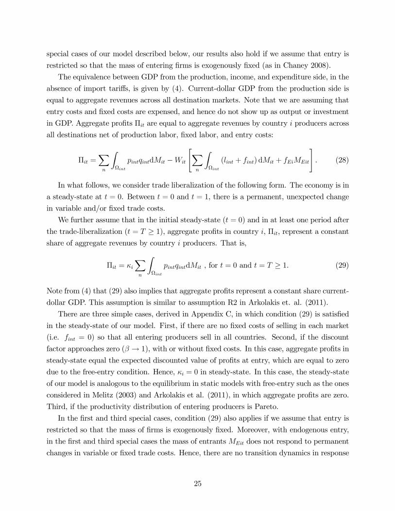
special cases of our model described below, our results also hold if we assume that entry is

restricted so that the mass of entering firms is exogenously fixed (as in Chaney 2008).

The equivalence between GDP from the production, income, and expenditure side, in the

absence of import tariffs, is given by (4). Current-dollar GDP from the production side is

equal to aggregate revenues across all destination markets. Note that we are assuming that

entry costs and fixed costs are expensed, and hence do not show up as output or investment

in GDP. Aggregate profits Π are equal to aggregate revenues by country producers across

all destinations net of production labor, fixed labor, and entry costs:

Π =X

ZΩ

d −

"X

ZΩ

( + ) d +

#. (28)

In what follows, we consider trade liberalization of the following form. The economy is in

a steady-state at = 0. Between = 0 and = 1, there is a permanent, unexpected change

in variable and/or fixed trade costs.

We further assume that in the initial steady-state ( = 0) and in at least one period after

the trade-liberalization ( = ≥ 1), aggregate profits in country , Π, represent a constant

share of aggregate revenues by country producers. That is,

Π = X

ZΩ

d , for = 0 and = ≥ 1. (29)

Note from (4) that (29) also implies that aggregate profits represent a constant share current-

dollar GDP. This assumption is similar to assumption R2 in Arkolakis et. al. (2011).

There are three simple cases, derived in Appendix C, in which condition (29) is satisfied

in the steady-state of our model. First, if there are no fixed costs of selling in each market

(i.e. = 0) so that all entering producers sell in all countries. Second, if the discount

factor approaches zero ( → 1), with or without fixed costs. In this case, aggregate profits in

steady-state equal the expected discounted value of profits at entry, which are equal to zero

due to the free-entry condition. Hence, = 0 in steady-state. In this case, the steady-state

of our model is analogous to the equilibrium in static models with free-entry such as the ones

considered in Melitz (2003) and Arkolakis et al. (2011), in which aggregate profits are zero.

Third, if the productivity distribution of entering producers is Pareto.

In the first and third special cases, condition (29) also applies if we assume that entry is

restricted so that the mass of firms is exogenously fixed. Moreover, with endogenous entry,

in the first and third special cases the mass of entrants does not respond to permanent

changes in variable or fixed trade costs. Hence, there are no transition dynamics in response

25

to permanent trade liberalization, and condition (29) holds for any time period ≥ 1. In allother cases with aggregate transition dynamics between steady-states, the share of profits in

revenues need not be constant along the transition paths. In these cases, our results hold

across steady-states.

Using (4) and (29), current-dollar GDP at time = 0 and any time period = in which

condition (29) holds is given by

=

1− . (30)

We now calculate changes in real GDP and real consumption between = 0 and any time

period = in which condition (29) holds.

Real GDP

We first calculate changes in real GDP based on aggregate deflators. The ratio of real GDP

between periods = 0 and = is given by

0

=

Y=1

µ−1−1

¶=

0

Y=1

µ1

−1

¶(31)

=1P

1 0

1,

which coincides with expression (9) in the previous models. In deriving expression (31), the

first step uses (2) and (8), the second step factors-out the ratios of current-dollar GDPs,

and the last step uses (6), (27), and (30). The expression for the change in real GDP using

disaggregated deflators (which, recall, is also the one resulting from using the direct valuation

method) is derived in a similar fashion, and coincides with expression (12) in the previous

models.

Note that, for given levels of trade shares by continuing producers, (which might

differ from overall trade shares due to entry and exit by firms into individual countries)

and for given changes in variable trade costs, −1, the change in real GDP in the

model with endogenous specialization and monopolistic competition is the same as in the

previous models. For given values of and −1, reallocation of production from

less productive to more productive producers (including exit by less productive producers

and entry into exporting by more productive producers) does not result in an additional

source of changes in aggregate productivity and real GDP. This is because value-added per

production worker of individual producers, which is related to real GDP by expression (10),

is equal to the ratio of the wage and the constant markup, independent of productivity of

individual producers.

26

Consider now changes in fixed costs or in the size of foreign countries when variable costs

are unchanged. While these can induce changes in the volume and revenue share of trade,

the ratio of PPIs is equal to0 and hence does not directly reflect the changes in fixed

costs. Real GDP from expression (9) is unchanged: 0 = 1. This result is

summarized in the following corollary to Result 1.21

Corollary to Result 1: In response to changes in fixed international trade costs between

any pair of countries, real GDP in each country is unchanged.

Real consumption and theoretical consumption

The expressions for changes in real consumption are the same as those in our baseline model:

(15) with aggregate deflators or (17) with disaggregated deflators. Together with the fact

that the expressions for changes in real GDP are also the same as in the previous models,

Result 4 on the equivalence, to a first-order approximation, between changes in world real

consumption and world GDP under trade balance holds.

What differs in this model is the comparison between real consumption and theoretical

consumption, country-by-country. Changes over time in the set of consumed varieties pro-

duces differences between real consumption and theoretical consumption beyond the stan-

dard substitution bias. In particular, while the CPI between any two time periods only

includes changes in prices of goods that are available for consumption in both periods, the

theoretical price index also reflects changes in the mass of consumed goods.

This implies that in the model with endogenous specialization and monopolistic compe-

tition, inequality (16) that bounds the difference between real consumption and theoretical

consumption does not apply since it is derived under the assumption that the set of available

goods for consumption is unchanged between time periods.22 Moreover, with changes in the

mass of consumed varieties, either from changes in the set of goods supplied domestically or

from changes in the set of goods imported from abroad, changes in the theoretical price index

are not equal to the CPI as defined in (14), even to a first-order approximation. Therefore,

Result 2, establishing the equality between changes in real consumption and theoretical con-

sumption country-by-country, does not apply immediately in this version of the model. For

example, an increase in the mass of consumed goods from abroad lowers the welfare-based

price index (and hence increases theoretical consumption), but does not directly change the

21There are interactions effects from changes in variables costs and changes in fixed costs on real GDP. For

example, a reduction in variable trade costs between countries and that is accompanied by a reduction

in fixed export costs can result in a larger trade share by continuing exporters at time 0 and hence lead

to a larger increase in real GDP.22Inequality (16) would hold if the CPI attributed a price equal to infinite to goods that are not available

for consumption.

27

CPI (and hence does not affect measured real consumption).

We show, however, that the equivalence between changes in real consumption and the-

oretical consumption in response to marginal changes in variable trade costs holds at the

world level. This result, which is derived in Appendix D, is summarized as follows:

Result 5: If each country has balanced trade, then steady-state changes in world real con-

sumption and theoretical consumption (defined as cross-country weighted averages of changes

in real consumption and theoretical consumption, respectively, using current-dollar GDP

weights) in response to changes in variable trade costs are equal, up to a first-order ap-

proximation, and both are given by expression (22).

Results 4 and 5 combined imply that, up to a first-order approximation, steady-state

changes in world real GDP and in world theoretical consumption in response to changes in

variable trade costs are equal, up to a first-order approximation.

Note that, given that expression (22) holds in all the models that we consider, we have

that for given trade shares and given marginal changes in variable trade costs, steady-state

changes in world real GDP, real consumption, and theoretical consumption are all equal

across these models up to a first-order approximation. This equivalence does not require any

parametric assumption on the productivity distribution of entering firms, (), as long as

our restriction (29) holds.

Result 5 can be understood as follows. Note that when countries are symmetric, this

result states that changes in real consumption equal changes in theoretical consumption in

response to marginal changes in variable trade costs. This is because, as discussed in Atkeson

and Burstein (2010), when countries are symmetric the indirect effect of a change in trade

cost on consumption through its effect on the set of consumed goods (due to changes in the

mass of entering firms and changes in exit and export thresholds, which are not captured

in the CPI) is zero up to a first-order-approximation. Hence, in each country changes in

the theoretical price index are approximately equal to changes in the CPI. With asymmetric

countries, changes in relative country sizes alter the equivalence between real consumption

and theoretical consumption, country-by-country, due to changes in the relative market size

of countries. This effect, however, washes-out across countries (i.e. the gain in one country

is a loss for another) when comparing steady-state changes in world real consumption and

world theoretical consumption.23

To establish the equality between real consumption and theoretical consumption, country-

23For this result to hold, it is important that fixed and entry costs are denominated in terms of labor.

If these costs entail a combination of labor and final good, then changes in the relative wage can result in

additional indirect effects from changes in the mass of consumed varieties on the welfare-based price index

that are not captured in the CPI (see the related discussion for welfare in Arkolakis et. al. 2011 and Atkeson

and Burstein 2010).

28

by-country, in response to changes in variable trade costs (as in Result 2), we must impose two

additional assumptions. First, fixed export costs are paid in the importing country. Second,

the distribution of productivities of entering firms, () is Pareto. These assumptions

are made in Eaton, Kortum, and Kramarz (2010) and for some results in Arkolakis et. al.

(2011).24 Under these assumptions, we obtain the following result that we prove in Appendix

E.

Result 6: Suppose fixed export costs are paid in the importing country, and that the

distribution of entering firms is Pareto. If each country has balanced trade, then steady-state

changes in real consumption and theoretical consumption in response to changes in variable

trade costs are equal country-by-country, to a first-order approximation.

Result 6 implies that, in response to marginal changes in variable trade costs, changes in

the mass and in the composition of consumed domestic and exported goods (due to changes

in exit and export thresholds) offset each other in each country’s theoretical price index.

Hence, changes in the CPI and in the theoretical price index coincide, up to a first-order

approximation. Note that this result does not require that the mass of consumed varieties

remains unchanged in each country (even though the mass of entering firms in each country

does). Indeed, reductions in marginal trade costs typically result in an increase in the mass

of consumed goods (which, however, does not affect the theoretical price index).

Numerical example

We illustrate how changes in real GDP, real consumption, and theoretical consumption

compare in a quantitative example of our model with monopolistic competition. We consider

small and large reductions in variable trade costs to evaluate the accuracy of some of our

equivalence results derived using first-order approximations. We consider a two-country

version of our model with trade balance, symmetric trade costs ( 12 = 21 = and

12 = 21), Pareto productivity distribution of entering firms with slope parameter of 5 (as

in Eaton, Kortum and Kramarz 2010, implying a trade elasticity equal to 5), and elasticity

of substitution equal to 3. Variable trade costs are fully incurred in each exporting country,

and fixed export costs are incurred in either the exporting country or the importing country

(in the latter case, the economy satisfies the assumptions in Result 6). We choose the

initial level of variable trade costs 0 = 147 and relative country sizes 12 = 205, so

that the goods’ trade share in country 1 is 120 = 7% and the trade share in country 2

24These assumptions are required for the "ex-ante" result of Proposition 2 in Arkolakis et. al. (2011).

Under these assumptions, their model responds to any global change in variable trade costs like an Armington

model. Given that the welfare-based prices in the Armington model behaves, to a first-order approximation,

like the CPI, we obtain the equivalence between real consumption and consumption-based welfare, country

by country.

29

is 210 = 15%. The share of each country in world GDP is 10 = 068 and 20 = 032,

respectively. The unchanged level of fixed costs do not affect our reported results. Recall

that in this specification, entry remains unchanged, so the economy immediately transits to

the new steady-state (at time = 1).

We consider reductions in variable trade costs, ranging from very small (corresponding

to our first-order approximations) to quite large ( falls from roughly 147 to 123 so that

the trade share more than doubles). Figure 1 considers the case in which fixed export costs

are paid in the exporting country and Figure 2 the case in which fixed export costs are paid

in the importing country. Based on the results in Arkolakis et. al. (2010), the specification

in which fixed export costs are incurred in the importing country is exactly equal to the

Armington version of our model with perfect competition and exogenous specialization and

to the Krugman version of our model with monopolistic competition but no fixed costs, both

parameterized with = 5.

In each figure, the x-axis displays the ratio of trade shares in the post- and pre-liberalization

periods, 10 and the y-axis displays the negative of the elasticity of real GDP, real con-

sumption, and theoretical consumption with respect to the change in variable trade costs

(e.g.. − log (10) log ( 1)). We report the measures of real GDP and real

consumption calculated based on disaggregated deflators, which minimize the standard sub-

stitution bias in response to large changes in trade costs. We report separately the responses

in each country and at the world level.

From Figures 1 and 2 we can observe that the higher order terms can be quite large.

That is, the elasticities of each aggregate variable are largely increasing in the size of the

reduction in trade costs. This implies that, for example, expression (21) is not a very accurate

approximation for large reductions in trade costs: the elasticity of world real GDP and world

real consumption is 10 ∗120+ 20 ∗210 ' 009 in response to a marginal reduction in tradecosts, and roughly 015 in response to a large reduction in trade costs that doubles the trade

share.

However, quite remarkably, theoretical and measured gains from trade are fairly close

even for large reductions in trade costs that result in large increases in trade shares. In

particular, first, the elasticity of world real GDP and the elasticity of world real consumption

are almost exactly equal for any size of the reduction in trade costs (Result 4).25 Second, for

large reductions in trade costs, the elasticity of world real consumption is only slightly higher

than the elasticity of world theoretical consumption (Result 5). Third, in each country (and

25For any change in trade costs, the increase in real GDP in country 1 (country 2) is slightly larger (smaller)

than the increase in real consumption in that country, reflecting the fact that the wage in country 1 rises

relative to the wage in country 2.

30

especially in country 2), for any size of the reduction in trade costs the elasticity of real

consumption is quite close to the elasticity of theoretical consumption. This is not only

the case when fixed export costs are incurred in the importing country (Result 6) but also

when fixed export costs are incurred in the exporting country (for which we do not have

an analytic result). Finally, comparing the elasticity of each variable in Figures 1 and 2 for

any given change in variable trade costs, both specifications have very similar quantitative

implications for both theoretical and measured aggregate gains from trade.

7 Two Extensions

In this section, we consider two extensions of our model. The first extension adds endogenous

quality choice by firms. The second extension introduces multiple factors of production. We

introduce these extensions in our model with monopolistic competition. We provide condi-

tions under which our previous results on the response of aggregate productivity to changes

in trade costs, and on the first-order equivalence between changes in real GDP, real con-

sumption, and theoretical consumption at the world level (or country-by-country for real

and theoretical consumption under stronger conditions) hold in the extended model. Details

are provided in Appendices F and G.

Endogenous quality choice

The final good is given by

=

∙ZΩ

()1 () ()

−1 d

¸ −1,

where () denotes the quality of differentiated good in country . The theoretical price

index is given by =hR

Ω () ()

1−di 11−. Higher levels of quality decrease the

price index.

Demand in country for good produced in country is given by

() = () ( () )−

. Higher quality increases demand, given prices. We

assume that each period, individual producers from country with productivity must em-

ploy (; ) units of labor in the home country to set quality for sales in country

, where (; ) is increasing and convex in .26 We assume that these costs are expensed,

so they are not included in GDP. Given that quality costs are independent of the volume

26We assume throughout that (; ) is such that the level of for active products is positive and bounded,

and so that in steady-state there is positive entry and a stationary size distribution. All our results hold if

is constrained to be equal across destination countries, with the exception of the equivalence between

real and theoretical consumption country by country, which requires that be destination specific.

31

of production, reductions in trade costs that raise the scale of exporters typically induce a

higher investment in quality by exporters relative to non-exporters.

The share of profits in GDP is constant in the steady-state (condition 29) under the two

following alternative assumptions. First, if the discount factor approaches zero ( → 1).

As → 1, aggregate profits, which now include the costs of quality choice, become zero

from the free-entry condition, so = 0 in steady-state. Second, if (; ) takes the form

(; ) =0 () and either (i) there are no fixed costs of supplying individual markets or

(ii) the productivity distribution of entering producers is Pareto. In Appendix F we derive

for this case.

Prices set by individual producers are given by expression (27) as in our baseline model.

A key consideration that determines the aggregate measured gains from trade is whether

deflators are constructed using prices adjusted for quality (i.e. () ()) or non-

adjusted for quality (i.e. ()).27

If prices in the PPI do not adjust for quality changes, then the expression for changes in

real GDP is equivalent to that in our baseline model without endogenous quality (expressions

8 and 12), derived using condition (29). If prices in the PPI do adjust for quality changes,

then if average quality rises in response to a reduction in trade costs, the PPI falls relative to

the scenario in which prices are not adjusted for quality changes. In this case, the increase

in real GDP (conditional on trade shares and changes in trade costs) is larger than the one

in expressions (8) and (12)

Consider now the response of real consumption. In Appendix F we establish the following

result. If prices in the CPI do not reflect changes in product quality, then changes in world

real consumption and world theoretical-consumption in response to marginal changes in

variable trade costs are equal, to a first-order approximation, and given by expression (22).

This equality also applies to world real GDP if GDP deflators do not adjust for quality

changes. Intuitively, the effects on the world welfare-based price index from changes in the

set of consumed goods (changes in the mass of entering firms and changes in exit and export

thresholds) and endogenous quality changes add up to zero, up to a first-order approximation.

If prices in the CPI do not capture any of these margins (i.e. prices are not adjusted for

quality changes), then the CPI coincides with the welfare-based price index.

Suppose instead that prices in the CPI do adjust for quality changes. If average quality

rises in response to a reduction in trade costs, the CPI falls relative to the baseline scenario

in which prices are not adjusted for quality changes, and measured gains in world real

27Product quality in this setup can be re-interpreted as producer productivity. In this case, producers

innovate to improve productivity rather than product quality. This re-interpretation does not change any of

the model’s implications for theoretical consumption. Note, however, that changes in productivity are more

likely to be captured in price indices, as when prices are adjusted for quality.

32

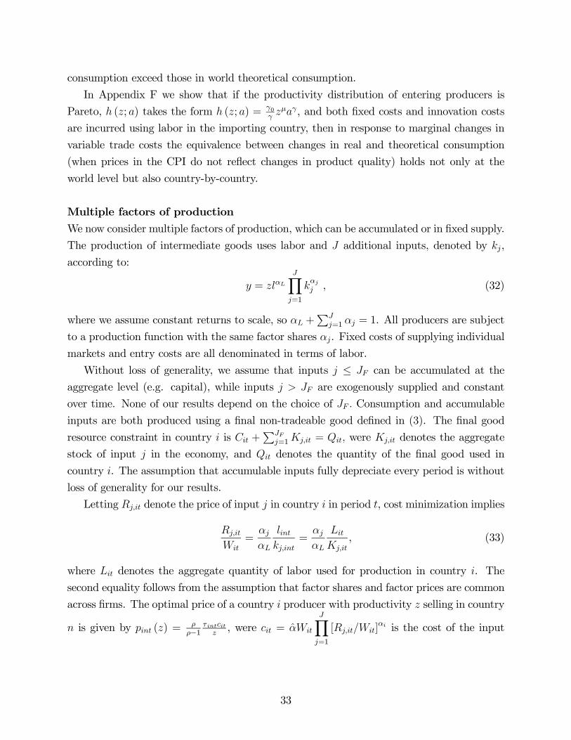
consumption exceed those in world theoretical consumption.

In Appendix F we show that if the productivity distribution of entering producers is

Pareto, (; ) takes the form (; ) =0, and both fixed costs and innovation costs

are incurred using labor in the importing country, then in response to marginal changes in

variable trade costs the equivalence between changes in real and theoretical consumption

(when prices in the CPI do not reflect changes in product quality) holds not only at the

world level but also country-by-country.

Multiple factors of production

We now consider multiple factors of production, which can be accumulated or in fixed supply.

The production of intermediate goods uses labor and additional inputs, denoted by ,

according to:

= Y

=1

, (32)

where we assume constant returns to scale, so +P

=1 = 1. All producers are subject

to a production function with the same factor shares . Fixed costs of supplying individual

markets and entry costs are all denominated in terms of labor.

Without loss of generality, we assume that inputs ≤ can be accumulated at the

aggregate level (e.g. capital), while inputs are exogenously supplied and constant

over time. None of our results depend on the choice of Consumption and accumulable

inputs are both produced using a final non-tradeable good defined in (3). The final good

resource constraint in country is +P

=1 = were denotes the aggregate

stock of input in the economy, and denotes the quantity of the final good used in

country . The assumption that accumulable inputs fully depreciate every period is without

loss of generality for our results.

Letting denote the price of input in country in period , cost minimization implies

=

=

, (33)

where denotes the aggregate quantity of labor used for production in country . The

second equality follows from the assumption that factor shares and factor prices are common

across firms. The optimal price of a country producer with productivity selling in country

is given by () =

−1

, were =

Y=1

[] is the cost of the input

33

bundle in country Using (33) we can rewrite as

=

Y=1

∙

¸. (34)

Real GDP: GDP includes output used for both consumption and accumulable inputs. We

calculate real GDP using aggregate deflators. We first calculate the aggregate PPI. Note

that, given that consumption and accumulable inputs use the same production technology,

there is a single PPI for final goods, given by (6), which can be written as:

−1=

P

RΩ

00

³

−1

´d0P

RΩ

00d0

=

−1

X

−1. (35)

In the Appendix, we show that in this version of the model, current dollar GDP is propor-

tional to aggregate labor payments. Hence, the ratio of real GDP in time to time = 0 in

response to a permanent trade liberalization at time = 1 is

0

=

0

Y=1

µ1

−1

¶=

0

Y=1

Ã1

−1

P

−1

!(36)

=

Y=1

∙

0

¸ 1P 1 0

1,

where the last step follows from equation (34). Given trade shares of continuing producers

and given changes in variable trade costs, the change in measured aggregate productivity

coincides with that in our baseline model with a single factor of production (i.e. expression

(8). Of course, growth in aggregate quantities of non-labor factors of production contributes

to growth in real GDP.

Note that accumulable inputs may also be interpreted as intermediate goods. In this

case, GDP differs from gross output as it excludes the use of intermediate inputs. However,

our assumptions imply that the share of value added in firms’ gross-output is constant, so

the expression for real GDP remains unchanged.28

World real GDP, consumption, and theoretical consumption: In Appendix G we derive the

equivalence between world theoretical consumption, world consumption, and world GDP, up

28We can also calculate real GDP using the double deflation method and obtain the same expression. The

key is that intermediate inputs are produced using the same technology as final goods, so they are deflated

using the same deflator (35) as that used to deflate gross output.

34

to a first order approximation, in response to marginal changes in variable trade costs (if

the set of consumed products is unchanged or if the distribution of entering firms is Pareto

and fixed costs are incurred in the importing country, the first-order equivalence between

real consumption and theoretical consumption holds country-by-country). A key step in the

analysis is that, under our assumptions, changes in trade costs do not change the steady-

state ratio of consumption to final output, , in each country. The actual magnitudes of

changes in world aggregates (for given trade shares and changes in trade costs) differ from

those in the baseline model due to endogenous changes in aggregate quantities of non-labor

factors of production.

8 Conclusions

In this paper we have studied the implications of trade liberalization for aggregate measures

of economic activity in a widely-used class of workhorse models of international trade. We

have characterized how in these models real GDP and real consumption, as calculated by

statistical agencies in the United States, respond to changes in variable trade costs, fixed

trade costs, and tariffs.

For the class of models that we consider, our conclusions can be broadly summarized

as follows. First, aggregate output measured by real GDP and aggregate productivity con-

structed using data on real GDP increase in response to reductions in trade costs inso-

far as prices used to construct deflators reflect these changes in trade costs. Real GDP

and aggregate productivity, however, do no capture the reallocation of production towards

more productive producers resulting from trade liberalization. Second, gains in theoretical

(welfare-based) consumption from reductions in variable international trade costs translate

into measures of real consumption when aggregating these measures across countries. Under

stronger but common assumptions in the literature, the equivalence between theoretical and

measured consumption also holds country-by-country. Differences between consumption de-

flators and welfare-based price indices in response to changes in variable trade costs, that

may arise from changes in the set of consumed varieties or changes in the quality of indi-

vidual products wash-out when treated jointly across all countries (or country-by-country

under stronger assumptions). Third, conditional on trade shares (of continuing producers)

and changes in variable trade costs, all the models we consider deliver approximately the

same measured aggregate gains from trade. The equivalence in measured gains from trade

arises due to the equivalence in the welfare implications of these models.

Our results establish a benchmark to understand how the extensive empirical evidence

on the link between trade and aggregate measures of economic activity can be interpreted

35

through the lens of workhorse trade models, and how the theoretical link between trade

and welfare in these models translates into observable aggregates. Our results should be,

however, treated with caution to the extent that the measurement procedures in individual

countries differ from those carried out in the United States and recommended by the United

Nations. Finally, the extent to which our results carry over to richer models featuring addi-

tional sources of gains from trade to the ones we considered, such as the endogenous response

of markups, remains an open research question.

REFERENCES

Alvarez, Fernando and Robert Jr. Lucas. 2007. "General Equilibrium Analysis of the

Eaton-Kortum Model of International Trade,” Journal of Monetary Economics, Vol. 54, No.

6, pp. 1726-68.

Anderson, James E. 1979. "A Theoretical Foundation for the Gravity Equation," Amer-

ican Economic Review, Vol. 69, No. 1, pp. 106-16.

Anderson, James E and Eric van Wincoop. 2004. "Trade Costs," Journal of Economic

Literature, Vol. 42. No. 3, pp. 691-751.

Arkolakis, Costas, Arnaud Costinot, and Andrés Rodríguez-Clare. 2011. "New

Trade Models, Same Old Gains?," forthcoming American Economic Review.

Bajona, Claustre, Mark J. Gibson, Timothy J. Kehoe, and Kim J. Ruhl. 2010.

“Trade Liberalization, Growth, and Productivity,” Mimeo, University of Minnesota.

Boskin Commission Report. 1996. "Toward a More Accurate Measure of the Cost of

Living.”

Broda, Christian, and David E. Weinstein. 2006. "Globalization and the Gains from

Variety," Quarterly Journal of Economics, Vol. 121, No. 2, pp. 541-585.

Bureau of Economic Analysis. 2009 "Updated Summary of Nipa Methodologies".

http://www.bea.gov/scb/pdf/2009/11%20November/ .

Bureau of Economic Analysis. 2009. "Concepts and Methods of the U.C. Input-Output

Accounts". http://www.bea.gov/national/pdf/NIPAhandbookch1-4.pdf.

Bureau of Labor Statistics. 2008. "Handbook of Methods".

http://www.bls.gov/opub/hom/homtoc.htm.

Chaney, Thomas. 2008. "Distorted Gravity: The Intensive and Extensive Margins of

International Trade," American Economic Review, Vol. 98, No. 4, pp. 1707-1721.

Dornbusch, Rudiger, Stanley Fischer, and Paul Samuelson. 1977. "Comparative

Advantage, Trade, and Payments in a Ricardian Model with a Continuum of Goods," Amer-

ican Economic Review, Vol. 67, No. 5, pp. 823-39.

36

Eaton, Jonathan and Samuel Kortum. 2002. "Technology, Geography, and Trade,"

Econometrica, Vol. 70, No. 5, pp. 1741-1779.

Eaton, Jonathan, Samuel Kortum, and Francis Kramarz. 2010. "An Anatomy of

International Trade: Evidence from French Firms," forthcoming Econometrica.

Feenstra, Robert C., 1994, “New Product Varieties and the Measurement of International

Prices,” American Economic Review, Vol. 84, No 1, pp. 157-177.

Feenstra, Robert C, Alan Heston, Marcel P Timmer, and Haiyan Deng. 2009.

"Estimating Real Production and Expenditures across Nations: A Proposal for Improving

the Penn World Tables," The Review of Economics and Statistics, Vol. 91, No. 1, pp.

201-212.

Feenstra, Robert, Marshall B. Reinsdorf, and Matthew J. Slaughter. 2008. "Ef-

fects of Terms of Trade Gains and Tariff Changes on the Measurement of U.S. Productivity

Growth," Mimeo. UC Davis.

Feyrer, James. 2009a. "Trade and Income — Exploiting Time Series in Geography," NBER

Working Paper 14910.

Feyrer, James. 2009b. "Distance, Trade, and Income: The 1967 to 1975 Closing of the

Suez Canal as a Natural Experiment," NBER Working Papers 15557.

Frankel, Jacob and David Romer. 1999. "Does Trade Cause Growth?," American

Economic Review, Vol. 89, No. 3, pp. 379—399.

Gopinath, Gita and Brent Neiman. 2011. "Trade Adjustment and Productivity in

Large Crises," Mimeo. Harvard University.

Grossman, Gene and Elhanan Helpman. 1993. "Innovation and Growth in the Global

Economy," MIT Press, Cambridge, Massachusetts.

Hausman, Jerry. 2003. "Sources of Bias and Solutions to Bias in the Consumer Price

Index," Journal of Economic Perspectives, Vol. 17, No. 1, pp. 23—44.

Kehoe, Timothy and Kim J. Ruhl. 2010. “Why Have Economic Reforms in Mexico

Not Generated Growth?,” Federal Reserve Bank of Minneapolis, Research Department Staff

Report 453.

Kehoe, Timothy and Kim J. Ruhl. 2008. “Are Shocks to the Terms of Trade Shocks

to Productivity?,” Review of Economic Dynamics, Vol. 11, No. 4. pp. 804-819.

Kohli, Ulrich. 2004. “Real GDP, Real Domestic Income, and Terms-of-Trade Changes,”

Journal of International Economics, Vol. 62, No. 1, pp. 83-106.

Krugman, Paul R. 1980. "Scale Economies, Product Differentiation, and the Pattern of

Trade," American Economic Review, Vol. 70, No. 5. pp. 950-959.

McCully, Clinton, Brian Moyer, and Kenneth Stewart. 2007. "A Reconciliation be-

tween the Consumer Price Index and the Personal Consumption Expenditures Price Index,"

37

Working Paper. Bureau of Economic Analysis.

Melitz, Marc. 2003. "The Impact of Trade on Aggregate Industry Productivity and

Intra-Industry Reallocations," Econometrica, Vol. 71, No. 6, pp. 1695-1725.

Mayerhauser, Nicole and Erich Strassner. 2010. "Preview of the Comprehensive

Revision of the Annual Industry Accounts," Survey of Current Business 21-34.

Pavcnik, Nina. 2002. "Trade Liberalization, Exit, and Productivity Improvements: Evi-

dence from Chilean Plants,” Review of Economic Studies, Vol. 69, No. 1, pp. 245-76.

Rodriguez, Francisco and Dani Rodrik. 2001. "Trade Policy and Economic Growth:

A Skeptic’s Guide to the Cross-National Evidence," NBER Macroeconomics Annual 2000,

Vol. 15, pp. 261-338. National Bureau of Economic Research, Inc.

Waugh, Michael. "International Trade and Income Differences," American Economic

Review, Vol. 100, No. 5, pp. 2093-2124.

38

1 1.1 1.2 1.3 1.4 1.5 1.6 1.7 1.8 1.9 2

0.06

0.07

0.08

0.09

0.1

0.11

0.12Country 1 (large)

Trade share, post/pre liberalization

−Δ

log

X /

Δ lo

g τ

Theoretical consumptionReal consumptionReal GDP

1 1.1 1.2 1.3 1.4 1.5 1.6 1.7 1.8 1.9 2

0.15

0.2

0.25

Country 2 (small)

Trade share, post/pre liberalization

−Δ

log

X /

Δ lo

g τ

Figure 1: Gains from reductions in variable trade costs, Fixed costs in exporting country

1 1.1 1.2 1.3 1.4 1.5 1.6 1.7 1.8 1.9 2

0.09

0.1

0.11

0.12

0.13

0.14

0.15

World

Average trade share, post/pre liberalization

−Δ

log

X /

Δ lo

g τ

39

1 1.1 1.2 1.3 1.4 1.5 1.6 1.7 1.8 1.9 2

0.06

0.07

0.08

0.09

0.1

0.11

0.12Country 1 (large)

Trade share, post/pre liberalization

−Δ

log

X /

Δ lo

g τ

Theoretical consumptionReal consumptionReal GDP

1 1.1 1.2 1.3 1.4 1.5 1.6 1.7 1.8 1.9 2

0.16

0.18

0.2

0.22

0.24

0.26Country 2 (small)

Trade share, post/pre liberalization

−Δ

log

X /

Δ lo

g τ

Figure 2: Gains from reductions in variable trade costs, Fixed costs in importing country

1 1.1 1.2 1.3 1.4 1.5 1.6 1.7 1.8 1.9 2

0.09

0.1

0.11

0.12

0.13

0.14

0.15

0.16World

Average trade share, post/pre liberalization

−Δ

log

X /

Δ lo

g τ

40

Appendix A: Substitution bias in the CPI

In this appendix we derive the well-know substitution bias on the CPI, establishing that the

Laspeyres (Paasche) price index overstates (understates) changes in the welfare-based price

index. We assume through this section that the same set of goods is consumed in all periods,

Ω = Ω and =. Note that we can write the Laspeyres price index as:

0

¯0=0

=X

Λ0

µ

0

¶,

where Λ =RΩ(d)

P

RΩ

d is country 0 share of expenditures on

goods produced in country at date Similarly, we can re-write the Paasche price index as:

0

¯0=

=

"X

Λ

µ0

¶#−1

The welfare-based price index is defined as:

= min

X

ZΩ

d : [ () ≥ ] .

Let ∗ denote the solution to this problem when prices are . The change in the welfare-

based price index is given by:

0

=

P

RΩ

∗dP

RΩ

0∗0d

≤P

RΩ

∗0dP

RΩ

0∗0d

=X

Λ∗0

µ

0

¶

where the inequality follows from the definitions of ∗ and Λ∗ =Ω

∗d

Ω

∗d

. Simi-

larly:

0

=

P

RΩ

∗dP

RΩ

0∗0d

≥P

RΩ

∗dP

RΩ

0∗d

=

"X

Λ∗

µ0

¶#−1. (A1)

If is homothetic (so that expenditure shares only depend on relative prices and do not

depend on income), then, Λ∗ = Λ, and (1) implies (16).

A-1

Appendix B: International specialization of shipping services

We first calculate the change in real GDP (using aggregate deflators) in country . The PPI

in period relative to period − 1 is given by

−1=

−1

"X

µ

−1

¶+X6=

X

µ − 1 −1 − 1

¶

#

where

=

RΩ

¡0 + 0

¢0d0P

RΩ

¡0 + 0

¢0d0 +

P6=

P

RΩ

00d0

and, for 6= ,

=

RΩ

00d0P

RΩ

¡0 + 0

¢0d0 +

P6=

P

RΩ

00d0

,

withP

+P

6=P

= 1. The ratio of real GDP in time period relative to − 1is

−1=

à −1

−1

!05Ã

−1−1

!05(A2)

=1P

³

−1

´+P

6=P

³ −1

−1−1

´ .Clearly, −1 1 if trade costs fall.

We now derive the change in world real GDP and real consumption under balanced trade.

Log-differentiating (2),

log = −X

log −X6=

X

− 1 log .

Together with log = 0 for 6= , and using the definitions of and , we

obtain expression (22), where for 6= is evaluated at prices inclusive of trade

services provided by country .

With balanced trade in each country, the world change in real consumption is, to a first-

order approximation, given by expression (20), where country-specific expenditures are

calculated inclusive of trade costs provided by country , and changes in country specific

A-2

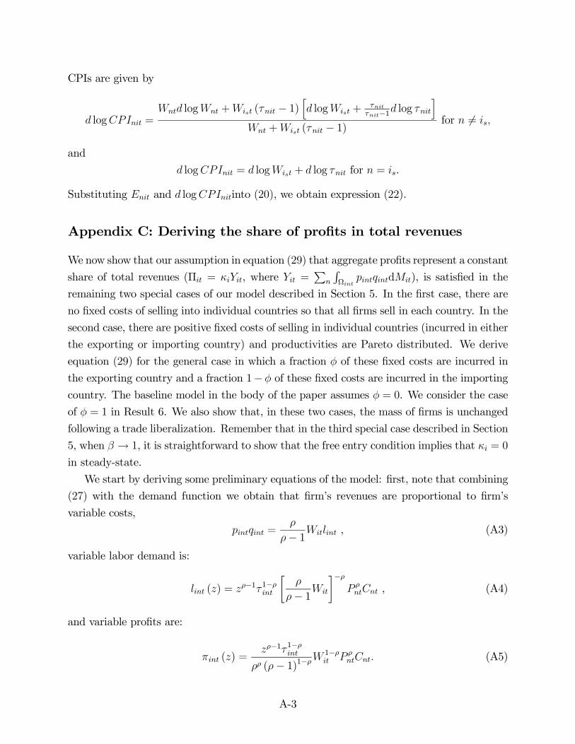
CPIs are given by

log = log + ( − 1)

h log +

−1 log

i + ( − 1)

for 6=

and

log = log + log for = .

Substituting and loginto (20), we obtain expression (22).

Appendix C: Deriving the share of profits in total revenues

We now show that our assumption in equation (29) that aggregate profits represent a constant

share of total revenues (Π = , where =P

RΩ

d), is satisfied in the

remaining two special cases of our model described in Section 5. In the first case, there are

no fixed costs of selling into individual countries so that all firms sell in each country. In the

second case, there are positive fixed costs of selling in individual countries (incurred in either

the exporting or importing country) and productivities are Pareto distributed. We derive

equation (29) for the general case in which a fraction of these fixed costs are incurred in

the exporting country and a fraction 1− of these fixed costs are incurred in the importing

country. The baseline model in the body of the paper assumes = 0. We consider the case

of = 1 in Result 6. We also show that, in these two cases, the mass of firms is unchanged

following a trade liberalization. Remember that in the third special case described in Section

5, when → 1, it is straightforward to show that the free entry condition implies that = 0

in steady-state.

We start by deriving some preliminary equations of the model: first, note that combining

(27) with the demand function we obtain that firm’s revenues are proportional to firm’s

variable costs,

=

− 1 , (A3)

variable labor demand is:

() = −1 1−

∙

− 1

¸− , (A4)

and variable profits are:

() =−1 1−

(− 1)1−1−

(A5)

A-3

In an equilibrium with selection by firms to sell in each country, there exists a threshold

such that only firms with ≥ operate in destination . That is, Ω = : ≥ .This threshold satisfies:

() =

1− . (A6)

Aggregate profits in country in period net of fixed labor costs and entry costs are given

by:

Π = − −X

1−

ZΩ

d −Ei ,

where denotes aggregate variable labor used in production, =P

RΩ

d. Note

that from expression (3), aggregate revenues are proportional to variable labor payments:

=

− 1 . (A7)

If condition (29) holds, then in combination with (30), we obtain

1

1− = =

− 1 ,

which implies that variable production labor is a constant share of total labor:

(1− )

− 1 = . (A8)

Hence, if aggregate profits represent a constant share of aggregate revenues, then aggregate

variable labor represents a constant fraction of total labor.

Suppose we are on a steady-state equilibrium in which aggregate variables are constant.

In steady-state, the interest rate is given by 1 and the distribution of firms is given by

() =

() (we omit time subscripts for the reminder of this section to simplify

notation). The aggregate free-entry condition in steady-state is:

=

1− [1− ]

" − −

X

1− [1− ()]

#. (A9)

In what follows, we solve for the constant of proportionality Π = = in steady-

state under two special cases of our model. We then show that, in these two special cases,

the aggregate response to a change in variable or fixed trade costs is immediate (i.e. there

are no transition dynamics), so that remains constant over time.

Case 1: No fixed costs

A-4

Assume that there are no fixed costs of selling in individual countries, i.e. = = 0 so

that there is no selection. In this case, the aggregate free entry condition (9) is:

=

1− [1− ][ −] ,

and using (7),

=

1− (1− )

1

. (A10)

Aggregate profits are:

Π = − −

= − − 1

−

1− [1− ]

1

=1−

[1− (1− )] ,

so = 1−(1−(1−)) Note that if 1, aggregate cross-sectional profits are positive even

though discounted profits at entry are zero.

The steady-state mass of entering firms is given by:

=

1− (1− )

(1− ),

where we used (7), (10), and equation (8). Hence, the mass of entrants does not

change in response to permanent changes in variable or fixed trade costs. Therefore, there

are no transition dynamics to the new steady-state, and = .

Finally, aggregate variable profits gross of entry costs are: Π+ = −1 Hence,

with restricted entry (so that there are no costs incurred in entry), equation (29) holds with

= 1.

Case 2: Pareto distributed productivities

Assume that there are positive fixed costs of selling in individual countries and that the

distribution of entering firms is Pareto with shape parameter , i.e. = 1 − − for

≥ 1. We also assume that the productivity cutoffs are interior, 1.We first show that aggregate fixed labor costs are proportional to aggregate revenues.

Using the Pareto form, we can rewrite the expression (6) that defines the cutoff as:

−1−

1−

1−

(− 1)1− =

1−

− (A11)

A-5

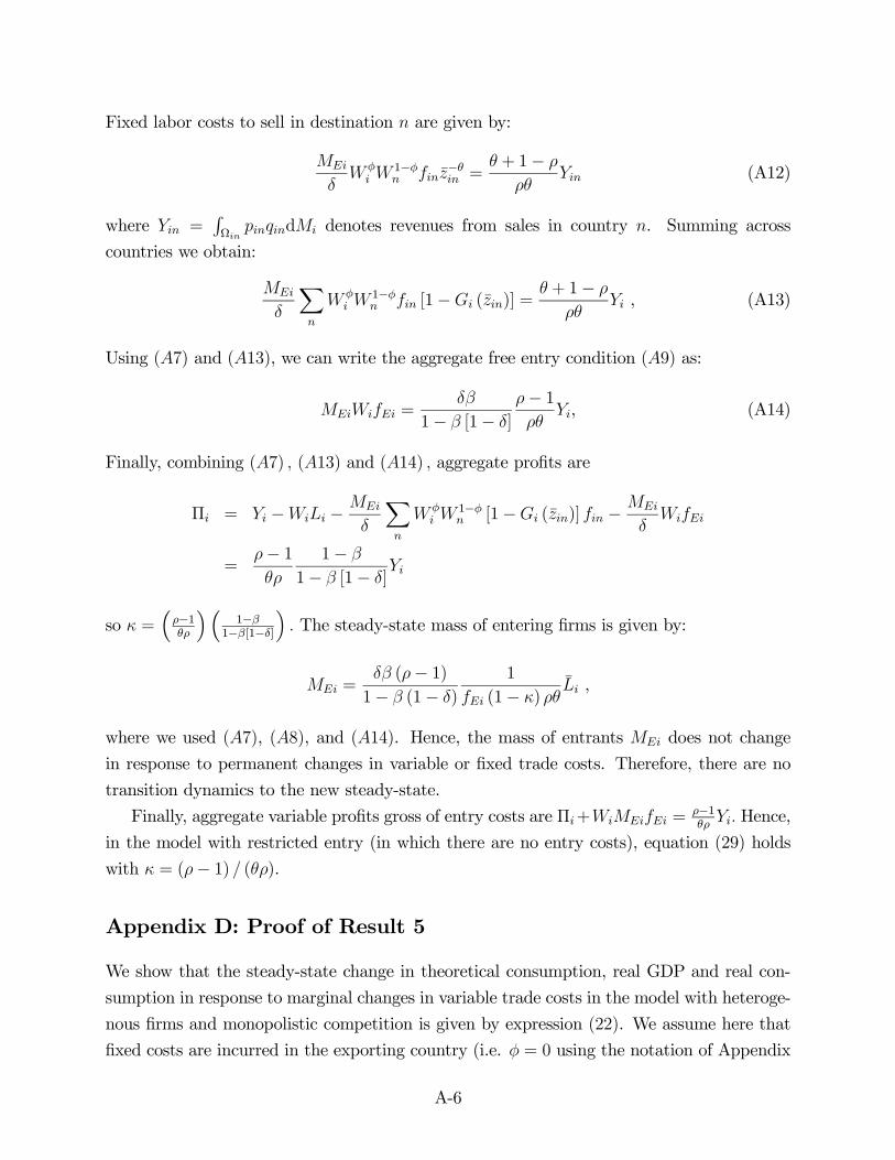
Fixed labor costs to sell in destination are given by:

1−

− =

+ 1−

(A12)

where =RΩ

d denotes revenues from sales in country . Summing across

countries we obtain:

X

1− [1− ()] =

+ 1−

, (A13)

Using (7) and (13), we can write the aggregate free entry condition (9) as:

=

1− [1− ]

− 1

, (A14)

Finally, combining (7) (13) and (14) aggregate profits are

Π = − −

X

1− [1− ()] −

=− 1

1−

1− [1− ]

so =³−1

´³1−

1−[1−]

´ The steady-state mass of entering firms is given by:

= (− 1)1− (1− )

1

(1− ) ,

where we used (7), (8), and (14). Hence, the mass of entrants does not change

in response to permanent changes in variable or fixed trade costs. Therefore, there are no

transition dynamics to the new steady-state.

Finally, aggregate variable profits gross of entry costs are Π+ =−1

Hence,

in the model with restricted entry (in which there are no entry costs), equation (29) holds

with = (− 1) ().

Appendix D: Proof of Result 5

We show that the steady-state change in theoretical consumption, real GDP and real con-

sumption in response to marginal changes in variable trade costs in the model with heteroge-

nous firms and monopolistic competition is given by expression (22). We assume here that

fixed costs are incurred in the exporting country (i.e. = 0 using the notation of Appendix

A-6

C).

Note first that we can re-express variable profits relative to the wage in equation (5) as

()

=−1 1−

(− 1)1−−

(A15)

=−1 1−

(− 1)1−µ

1−

¶

1−

where =

. In deriving this expression, we have used

=

(1− ) from (30)

and balanced trade.

Expected variable profits (relative to the wage) per entering firms are

X

ZΩ

()

d () =1

(− 1)1−µ

1−

¶

1−

X

1− , (A16)

where =RΩ

−1d. Free-entry in steady-state implies:

X

ZΩ

()

d () = + X

[1− ()] ,

where =

1−(1−) Log-differentiating this expression with respect to changes in τ around

the initial steady-state at time , and using (16) yields

log = −P

h log − 1

−1 logi1− P

1−

. (A17)

Here we have used an envelope condition to obtain that changes in cutoffs , defined by

(6), have no first-order effects on expected profits at entry. Using =1−

1−

, we

can re-write this expression as

log = −X

log +1

− 1X

log.

The change in world theoretical consumption using weights = P

, and using

= from trade balance, is given by

X

log =X

"−X

log +1

− 1X

log

#.

Using balanced trade (which implies P

= P

), and log = − log,

A-7

we haveP

P

log = 0, soX

log = −X

X

log .

Substituting the definition of , we obtain expression (22).

We now calculate the change in world real GDP to marginal changes in variable trade

costs. The aggregate PPI defined in (6) between − 1 and , using (11), is given by

−1=X

−1.

Log-differentiating around τ = τ 0,

log =X

log +X

=X

log

where we usedP

= 1 (which impliesP

= 0). Changes in trade shares by

continuing producers have no first-order effects on the PPI. Hence, the change in the PPI

is to a first-approximation equal to that in the model with a fixed set of producers selling

in each country. Following the steps used in the model with exogenous specialization, the

change in world real GDP is given by expression (22).

Finally, consider changes in real consumption. From equation (14), and the definition of

−1, the aggregate in country between period − 1 and is given by:

−1=X

Λ

−1,

where Λ =RΩ

00d0hP

RΩ

00d0

iis the date 0 share of country ’s

expenditures on goods from country for goods that are consumed in both periods. Note

that with a constant set of consumed goods, Λ = 00. Log-differentiating around

τ = τ 0,

log =X

log +X

Λ

=X

log,

A-8

where we usedP

Λ = 1 (which impliesP

Λ = 0). Changes in expenditure shares

due to changes in the set of consumed goods have no first-order effects on the CPI. Hence,

the change in the CPI is to a first-approximation equal to that in the model with a fixed set

of consumed goods. Following the steps used in the model with exogenous specialization,

the change in world real consumption under balanced trade is given by expression (22).

Appendix E: Proof of Result 6

We now show our Result 6 on the equivalence between real consumption and theoretical

consumption, country-by-country, when fixed cost of exporting are paid in the destination

country ( = 1 in the notation of Appendix C), and the productivity distribution of entering

firms is Pareto ( () = 1− − for ≥ 1). We assume that trade is balanced every period,taking into account the export of goods and the export of fixed trade costs that foreign firms

incurred in the domestic economy.

We start by showing that with Pareto distributed productivities, balanced trade in any

country implies balanced trade both in fixed export cost services and in goods in that country.

The condition of balanced trade in country is:

X6=

+X6=

[1− ()] =

X6=

+X6=

[1− ()] .

(A18)

Substituting (12) into (18) implies:X6=

=X6=

, (A19)

which is the condition of balanced trade in goods.

We now derive Result 6. Balanced trade in services implies = . Then, log-

differentiating equation (30) with respect to changes in τ around the initial steady-state at

time yields:

log =X

log = 0 (A20)

Using

=

(1− ) from (30) and balanced trade in goods we can re-express as:

=

ZΩ

d

=

1−

1− ,

A-9

where ≡³

1−

´£−1 [− 1]1−¤ and =

as in Appendix D. Log-differentiating

we obtain:

log = (1− ) log + log (A21)

+ log + (1− ) log ,

substituting into (20), we can write the change in welfare based consumption as:

log = −X

∙ log +

log

1− +

log

1−

¸.

Log-differentiating (19), substituting (21) and some algebra gives:

X

∙ log +

log

1− +

log

1−

¸=X

∙ log + log

+ log

1−

¸,

then:

log = −X

∙ log + log

+ log

1−

¸. (A22)

Finally, using the Pareto form for , we have:

=

+ 1− −1− , (A23)

log differentiating (11) and (23) we obtain:

log = (− 1− ) [ log + log + log] . (A24)

Substituting (24) into (22) and using balanced trade in goods:

log = −X

[ log + log] ,

where = .

As shown in Appendix D, the change in the CPI is given by log =P

log

so the change in real consumption is given by expression (18) Substituting log in

equation (18) we obtain:

log =X

[− log − log] (A25)

A-10

which coincides with log.

Appendix F: Endogenous quality choice

In this appendix we consider the extended model with endogenous quality choice under en-

dogenous specialization and imperfect competition. We first derive the result that, if prices

in the deflators are not adjusted for changes in quality, then changes in world real consump-

tion and theoretical consumption are equal, to a first-order approximation, in response to

marginal changes in trade costs. The logic to obtain this result is very similar to that used to

obtain Result 5 in Appendix D. Next, we derive condition (29) in this version of our model.

Following the same steps as those used to derive expression (15), variable profits (rela-

tive to the wage) for a firm from country with productivity selling in country are given

by

()

= ()

−1 1−

(− 1)1−µ

1−

¶

1− ,

where () denotes the quality choice of a firm in country with productivity selling

in country in period . In an interior equilibrium with selection, the cutoff is given

by()

− − (; ()) = 0. Profits (relative to the wage) in period across all

destinations, inclusive of fixed costs and quality costs are given by

X

I ( ≥ )

∙ ()

−1 1−

(− 1)1−µ

1−

¶

1− − − (; ())

¸

where I ( ≥ ) = 1 if ≥ and zero otherwise. The static first-order condition for

() is given by

−1 1−

(− 1)1−µ

1−

¶

1− − 2 (; ) = 0,

where 2 (; ) denotes the derivative of with respect to the second argument.

The free-entry condition in steady-state is given by

X

ZΩ

()

() = +X

[1− ()] +

ZΩ

(; ()) () . (A26)

Log-differentiating the free-entry condition in the steady-state, using the first-order condi-

tions for and (), we obtain the same expression for the change in theoretical con-

sumption, (17), as in the model without quality choice, where =RΩ

() −1d.

That is, from the envelope conditions, changes in cutoffs and quality choices have no first-

A-11

order effects on expected profits of entering firms. From expression (17), we use the same

steps as those used in Appendix D to obtain expression (22).

The extension of Result 6 (the equivalence between real consumption and theoretical

consumption, country-by-country) under stronger assumptions, is derived in the Online Ap-

pendix.

Deriving the share of profits in total revenues

Deriving assumption (29) when → 1 is straightforward. We now show that this assump-

tion holds if 1 when productivites are Pareto distributed, quality is destination-country

specific, the cost of choosing quality for a firm with productivity is ( ) =0 () ,

and a fraction of the innovation costs are incurred in the source country and the remaining

fraction (1− ) are incurred in the destination country. We omit time subscripts to simplify

notation.

Under these assumptions, the optimal quality choice for a firm with productivity

satisfies:

() = 0

1− ()

()

Aggregate innovation costs, using the optimality condition and =1

−1, are:

X

ZΩ

0

1− ()

() () =

1

(− 1)

X

ZΩ

() ()

=1

(− 1)

The relation between variable and fixed labor costs is still given by equation (13). Aggregate

entry costs, calculated using (26), (7) and (13), are

=

1− (1− )

" − −

P

0

1−

RΩ

() () ()

−P

1− [1− ()]

#

=

1− (1− )

(− 1)−

1

− 1. (A27)

Finally, combining (7) (13) and (27) aggregate profits are

Π = − −

−

"X

0

1− [1− ()] +

X

1−

ZΩ

() () ()

#

= (− 1)−

1−

1− (1− )

A-12

Therefore, =³(−1)−

´³1−

1−(1−)

´ The steady-state mass of entering firms is given by

=

1− [1− ]

[− 1]−

(1− )

where we used (7), (8), and (27). Hence, the mass of entrants does not change

in response to permanent changes in variable or fixed trade costs. Therefore, there are no

transition dynamics to the new steady-state.

Finally, aggregate variable profits gross of entry costs are Π + =(−1)−

Hence, in the model with restricted entry (so that there are no entry costs), equation (29)

holds with = [ (− 1)− ] .

Appendix G: Multiple factors of production

In this appendix we derive some results in the extension of the model that allows for multiple

factors of production. We first show that GDP is proportional to total labor payments, and

we then derive the equivalence between world real GDP, real consumption, and theoretical

consumption. As in the baseline model, we assume that condition (29) is satisfied — it is

straightforward to extend the proofs in Appendix C to this extension—.

We first show that production labor is proportional to aggregate labor supply, and that

current-dollar GDP is proportional to aggregate labor payments. We also show that theo-

retical consumption is proportional to the aggregate production of the final good. We can

write a modified version of equation (3) as

=

− 1−1 ,

where we used (33) and the production function. Total revenues of active firms in coun-

try are given by =

−1, where denotes aggregate labor used in variable

production defined above. In the presence of intermediate inputs, total revenues are given

by:

= +Π +

X=1

.

In combination with (29) this implies, =1

1−

h +

P

=1

i or

=

1−

"

+X

#=

1−

∙

+1−

¸.

A-13

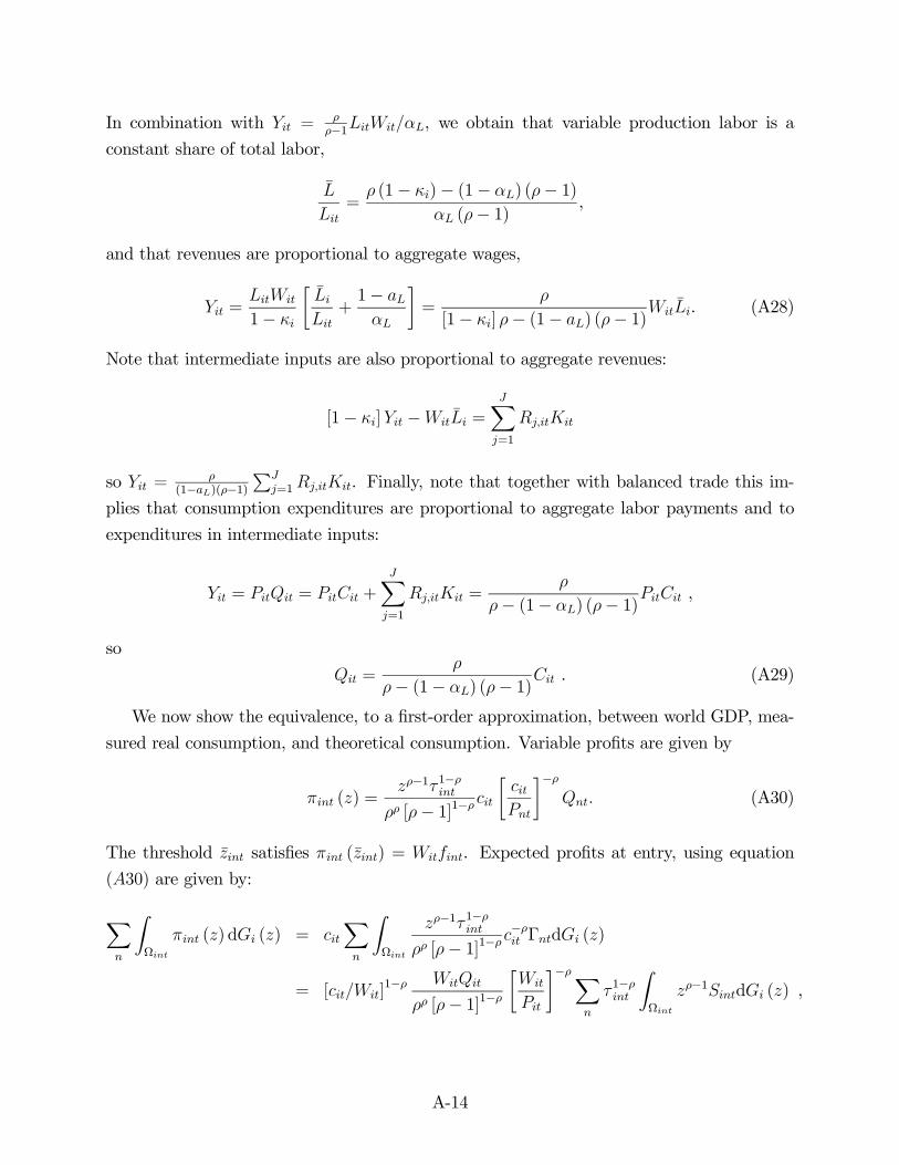
In combination with =

−1, we obtain that variable production labor is a

constant share of total labor,

= (1− )− (1− ) (− 1)

(− 1) ,

and that revenues are proportional to aggregate wages,

=

1−

∙

+1−

¸=

[1− ] − (1− ) (− 1). (A28)

Note that intermediate inputs are also proportional to aggregate revenues:

[1− ] − =

X=1

so =

(1−)(−1)P

=1. Finally, note that together with balanced trade this im-

plies that consumption expenditures are proportional to aggregate labor payments and to

expenditures in intermediate inputs:

= = +

X=1

=

− (1− ) (− 1) ,

so

=

− (1− ) (− 1) . (A29)

We now show the equivalence, to a first-order approximation, between world GDP, mea-

sured real consumption, and theoretical consumption. Variable profits are given by

() =−1 1−

[− 1]1− ∙

¸− (A30)

The threshold satisfies () = . Expected profits at entry, using equation

(30) are given by:

X

ZΩ

() d () = X

ZΩ

−1 1−

[− 1]1− − Γd ()

= []1−

[− 1]1−∙

¸−X

1−

ZΩ

−1d () ,

A-14

where Γ = , and =

ΓΓ. Using (28) and (29) we can write this as:

X

ZΩ

d () =

[]1−

1−

[− 1]1−X

1−

ZΩ

−1d () , (A31)

where =

−1[[1−]

−1−1+]−

[1(−1)+]1− is a constant. Free-entry in steady-state implies:

X

ZΩ

() d () = + X

[1− ()] ,

which can be rewritten as

[]1−

1−

[− 1]1−X

1− =

+X

[1− ()] .

Log-differentiating this expression in steady-state at time and using the envelope condition

for the cutoffs yields

log = −P

h log − 1

−1 logi1− P

1−

− log [] .

Note that =1−

1−

so the change in world theoretical consumption using the

weights defined above is:

X

log =X

"−P log

+ 1−1

P log − log

#.

Following the steps in Appendix C, we can show thatP

P

log = 0 which

implies: X

log = −X

"X

log + log

#.

Log differentiating the expression in (36) and doing the weighted sum across countries we

obtain the equivalence, to a first-order approximation, between world theoretical consump-

tion and world real GDP. To show the equivalence between world real GDP and world real

consumption we follow the same steps used in our baseline model, together with the fact

that current-dollar GDP is proportional to current-dollar consumption.

Note that the expression for the change in world real GDP, real consumption, and theo-

retical consumption differs from that in the model with only labor as a factor of production,

A-15

in the presence of changes in the marginal cost to wage ratio, . From expression (34),

changes in this price ratio are driven by changes in aggregate quantities of non-labor factors

of production.

The extension of Result 6 (the equivalence between real consumption and theoretical

consumption, country-by-country) under stronger assumptions, is derived in an Online Ap-

pendix.

A-16