buyout activity: the impact of aggregate discount rates · buyout activity: the impact of aggregate...
TRANSCRIPT

This paper presents preliminary findings and is being distributed to economists
and other interested readers solely to stimulate discussion and elicit comments.
The views expressed in this paper are those of the authors and are not necessarily
reflective of views at the Federal Reserve Bank of New York or the Federal
Reserve System. Any errors or omissions are the responsibility of the authors.
Federal Reserve Bank of New York
Staff Reports
Buyout Activity: The Impact of
Aggregate Discount Rates
Valentin Haddad
Erik Loualiche
Matthew C. Plosser
Staff Report No. 606
March 2013
Revised August 2015
Buyout Activity: The Impact of Aggregate Discount Rates
Valentin Haddad, Erik Loualiche, and Matthew C. Plosser
Federal Reserve Bank of New York Staff Reports, no. 606
March 2013; revised August 2015
JEL classification: G11, G23, G34
Abstract
Buyout booms form in response to declines in the aggregate risk premium. We document that the
equity risk premium is the primary determinant of buyout activity rather than credit-specific
conditions. We articulate a simple explanation for this phenomenon: a low risk premium
increases the present value of performance gains and decreases the cost of holding an illiquid
investment. A panel of U.S. buyouts confirms this view. The risk premium shapes changes in
buyout characteristics over the cycle, including their riskiness, leverage, and performance. Our
results underscore the importance of the risk premium in corporate finance decisions.
Key words: buyouts, discount rates, illiquidity, governance
_________________
Haddad: Princeton University (e-mail: [email protected]). Loualiche: Northwestern
University (e-mail: [email protected]). Plosser: Federal Reserve Bank of New York
(e-mail: [email protected]). For helpful comments, the authors thank Douglas
Diamond, Steven Kaplan, Anil Kashyap, Ralph Koijen, Adair Morse, Dimitris Papanikolaou,
Jonathan Parker, Pietro Veronesi and participants in the Chicago Booth Junior Finance
Symposium, SITE, the European Summer Symposium in Financial Markets, the Northwestern
Finance Conference, the Chicago Booth Finance Brownbag, the Economic Dynamics Working
Group at the University of Chicago, the Student Seminar and Macro Lunch at Northwestern
University, and the Transatlantic Doctoral Conference, London Business School. They also
appreciate research assistance from Tara Sullivan and Meru Bhanot. The views expressed in this
paper are those of the authors and do not necessarily reflect the position of the Federal Reserve
Bank of New York or the Federal Reserve System.
1 Introduction
Since their emergence in the 1980s, buyouts have been a powerful means to alter incentives
in firms. But the use of this transaction varies widely over time. In the U.S., peak years
experience close to one hundred public-to-private buyout transactions and trough years as
few as ten. We propose a simple explanation for these fluctuations: buyout activity responds
to changes in the aggregate risk premium. The discount rate affects firm valuations, and
therefore the decision to engage in a transaction. We document that this integrated view
of capital markets provides a detailed and powerful account of the cycle of buyout activity.
Our elementary explanation is in stark contrast to the existing literature that focuses on the
role of credit specific conditions.
Empirically, variation in buyout activity is better explained by changes in the risk pre-
mium than credit-market-specific conditions. Figure 1 illustrates how buyout activity de-
creases when the aggregate risk premium is high and increases when it is low. This factor
alone explains over 30% of the total variation in activity, more than three times the variation
explained by credit market conditions. To derive additional testable hypotheses at the firm
level, we present a model linking the buyout decision to a single time varying cost of capital.
We show that the characteristics of buyout targets and their variation across episodes of
high and low risk premium uniquely reflect our mechanism.
We investigate the impact of the risk premium on buyout decisions through the central
trade-off of performance gains versus the cost of providing incentives. In particular, a buyout
brings better management to the firm at the cost of compensating the acquirer for holding
skin in the game. The risk premium affects both sides of this trade-off. On the performance
side, the gains are muted when the risk premium is high: following the Gordon-growth model
intuition, the gains of a buyout increase with the difference between the firm’s growth rate
and the discount rate.1 On the other hand, providing incentives to the acquirer is costly:
she has to bear excess risk to be duly motivated to implement changes at the target. When
the risk premium increases, i.e. when the marginal willingness to bear risk decreases, the
willingness to bear this excess risk also decreases and compensating the acquirer becomes
more costly.
1The net present value of a cash-flow stream starting at X , growing exponentially at rate g and discountedat rate r is X/(r − g).
1

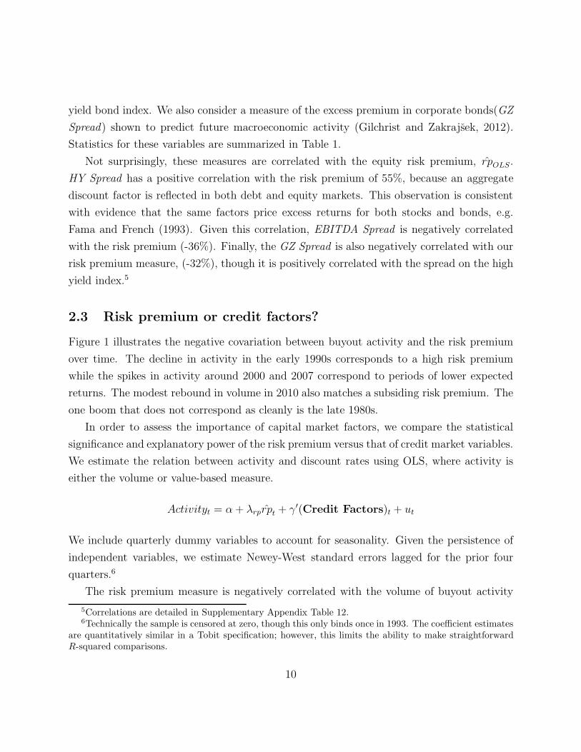
Figure 1: Time-Series of Buyout Volume and Aggregate Risk Premium
−10
−5
0
5
10
15
Ret
urn
%
0
10
20
30
Vol
ume
1985q1 1990q1 1995q1 2000q1 2005q1 2010q1
Quarter
Deal VolumeEquity Risk
Figure 1 illustrates quarterly deal volume of buyout transactions. The equity risk premium is predictedusing annual returns for a three-year period using D/P , cay, and the three-month T-bill as factors.
Using a panel of non-strategic, public-to-private deals from 1982 to 2011, we document
a novel set of facts regarding the quantity and nature of buyout activity. Our simple expla-
nation, focused on the risk premium, provides a unified explanation of these facts, whereas
credit-centric hypotheses are difficult to reconcile with our results. At the aggregate level,
buyout activity is negatively related to market-wide risk premium. This relation is robust to
the inclusion of market signals corresponding to common hypotheses in the literature: credit
market specific conditions (Axelson et al., 2013) or measures of debt-equity mispricing (Ka-
plan and Stromberg, 2009). The risk premium explains as much as 30% of the variation in
activity whereas credit factors alone only explain up to 10%. Consistent with our emphasis
on fundamental conditions, the market expected growth is also positively related to buyout
activity. Finally, our theory rationalizes the correlation between buyout activity, leverage,
2
deal pricing, and subsequent returns, documented for instance in Axelson et al. (2013).
While these aggregate facts strongly suggest the risk premium is the primary driver of
buyout activity, we also exploit the cross-section of firms to further distinguish the risk
premium from alternative hypotheses. First, riskier firms have a higher cost of capital and
greater illiquidity costs, making them undesirable buyout targets. In the panel, we confirm
the propensity of a firm to be bought out is sensitive to risk characteristics. Firms with high
market beta or high idiosyncratic volatility are less likely targets.
Going further, the role of risk characteristics varies over time. The greater the systematic
risk of the firm (i.e. beta), the more sensitive the cost of capital is to changes in the
risk premium. In addition, the illiquidity costs of high beta firms are more sensitive to
changes in the risk premium. Hence, among buyout targets, we expect fewer high beta
firms when the risk premium is high. Congruent with this prediction, we show that the
distribution of buyout firms’ betas shifts towards lower values during high risk premium
periods. In contrast, the idiosyncratic risk of buyout targets does not change with the risk
premium – a fact consistent with our theory. These results distinguish our thesis from an
explanation premised on changes in debt capacity which predicts that both systematic risk
and idiosyncratic risk will vary with the buyout cycle.
A second battery of tests focuses on the the impact of the risk premium in the cross-section
of firms. Firms with greater potential performance improvements should be more sensitive
to the risk premium. We find evidence to this effect by proxying for higher potential gains
using measures of agency problems: a corporate governance index, a measure of industry
competition and a cash-flow proxy. Firms with poor corporate governance are more sensitive
to changes in the risk premium, as are firms with more potential for a “free cash-flow”
problem. In addition, our framework concludes that it is less costly to compensate the
acquirer when it is easier to resell the firm, therefore the buyout activity of more liquid firms
should be less sensitive to changes in the risk premium. We measure the ease of exit for
acquirers using average industry-level M&A or IPO transaction activity and find more liquid
industries are less sensitive to movements in the risk premium. These results are robust to
the inclusion of credit market controls. The evidence confirms a unique role for the aggregate
risk premium in shaping the costs and benefits of buyout activity.
The fundamental tradeoff we emphasize for buyouts is standard in corporate finance and
can be generalized to other corporate transactions. We document the correlation between
3
deal activity and the risk premium for M&A and IPO activity. M&A activity responds
negatively to the risk premium, but less so than buyouts. This behavior is consistent with
the view that the performance channel matters for M&A deals but that buyouts are also
subject to the illiquidity channel which increases their sensitivity. For IPOs, the model
suggests the two channels conflict; we do not find a strong response to the risk premium
empirically.
Our paper’s emphasis on aggregate discount rates is unique in the buyout literature. Ka-
plan and Stromberg (2009) outline the history of aggregate private equity activity, but a
systematic explanation for buyout waves has remained elusive. Closest to us, Martos-Vila
et al. (2012) provide an explanation for the dynamics of financial versus strategic acquisition
activity. Their analysis focuses on mispricing in the debt market rather than changes in ag-
gregate prices. These explanations are not mutually exclusive. Both aggregate fundamentals
and relative mis-valuation can play a role. Motivated by our empirical findings, Malenko
and Malenko (2014) provide an alternative theoretical model for the role of variation in risk
premium for buyout activity. Rather than our basic tradeoff, they emphasize the ability of
private-equity-owned firms to borrow against their sponsors’ reputation with creditors and
externalities in sponsor reputation due to club formation.
A number of papers isolate specific events that impact buyout activity. Shivdasani and
Wang (2011) use cross-sectional evidence to argue that the advent of structured credit im-
proved access to capital for buyout investors. Similarly, the emergence of the high-yield
market likely stimulated activity, as Kaplan and Stein (1993) observe important changes in
the structure of deals during this period. Particular innovations in financial markets indeed
matter. For instance, discount rates fail to capture the intensity of the boom in the 1980s.
Nevertheless, aggregate forces are first order contributors to oscillations in activity, and they
should be considered as such when quantifying other hypotheses.
The literature on cross-sectional determinants of buyouts is more developed (Bharath
and Dittmar (2010), Opler and Titman (1993)), but few papers focus on risk measures.
Ewens et al. (2013) emphasize the role of exposure to diversifiable risk in the private equity
decision. Sorensen et al. (2013) consider the pricing of idiosyncratic risk by limited partners
(LPs) and build corresponding performance measures. In the context of this cross-sectional
literature, we highlight that the role of these characteristics, influenced by changes in the
4

aggregate risk premium, varies strongly over the cycle.
Our underlying theory of a buyout relies on an agency conflict between the LPs and the
general partners of a fund. Our model is parsimonious and designed to emphasize the role
of the aggregate risk premium. Axelson et al. (2009) provide an in-depth analysis of the
role of agency frictions in shaping buyout contracts and investments. Others have followed
a similar approach (Martos-Vila et al. (2012), Ewens et al. (2013) or Malenko and Malenko
(2014)), but their analysis does not consider aggregate discount rates.
More generally, we contribute to the broader literature emphasizing the role of time-
varying discount rates for corporate decisions. This literature is based on the insight that
changes in discount rates affect the cost of capital, which is an important parameter for eval-
uating investments. Time variation in the discount rate has been shown to affect investment,
as in Barro (1990), Cochrane (1991) and Berk, Green, and Naik (1999), and other forms of fi-
nancial activity (for a survey see Cochrane (2011)). For instance, Pastor and Veronesi (2005)
consider the role of pricing conditions for initial public offerings. This paper is the first to
apply this idea to buyout activity. Furthermore, we introduce a novel channel through which
changes in the aggregate risk premium impact financial decisions, our illiquidity channel.
2 The aggregate dynamics of buyout activity
We outline our main hypothesis on the role of the aggregate cost of capital and contrast it
with the credit market view. We describe the cyclical properties of buyouts and examine
their relation to capital markets conditions. The results document that a high aggregate
risk premium is a strong negative predictor of buyout activity and has greater explanatory
power than the relative cost of debt.
2.1 Potential determinants of buyout activity
Aggregate discount rates. An important empirical fact about capital markets is that
the cost of risky capital, or the risk premium, varies over time (Fama and French (1988),
Campbell and Shiller (1988a)). Consistent with integrated capital markets, this variation
is coordinated across types of financing, debt and equity (Fama and French (1989)). A
buyout is a type of investment generating operational changes in the firm (e.g. Davis et al.
5

(2014)). When the risk premium is large, future gains from investment are discounted more
and investment is less attractive (e.g. Barro (1990)). Also, concentrated, illiquid positions –
like those involved in buyout transactions – are particularly unattractive to investors when
the risk premium is high. These two forces predict a negative association of buyout activity
and prices with the risk premium.
The empirical importance of this hypothesis for buyout activity is the main conclusion
of our paper. We develop further testable hypotheses related to this mechanism in Section
3.
Credit market conditions. In contrast to this simple approach, a more commonly em-
phasized factor in the buyout decision is the cost of debt rather than common changes in the
cost of capital, e.g. Axelson et al. (2013). Underlying this view is the notion that buyout
investors exploit a mispricing in securities markets such that low borrowing costs facilitate a
transfer to buyout investors in the vein of Baker and Wurgler (2002). Another motivation is
that buyout investors, to mitigate overinvestment tendencies, can only raise debt once they
have obtained initial funding from their limited partners; therefore they are particularly
sensitive to the cost of debt (Axelson et al., 2009). When debt is “cheap”, transforming
equity-financed firms into debt-financed firms is more profitable, thus buyouts are more at-
tractive to investors. This view has implications for both the intensive and extensive margin
of deals. On the intensive margin, conditional on a deal occurring cheaper credit should co-
incide with greater deal leverage and higher takeout valuations. As for the extensive margin,
advantageous credit conditions should correspond to periods with more buyout activity.
The extant literature on buyouts has primarily tested implications on the intensive margin
of this theory. Most prominently, Axelson et al. (2013) relate the price and leverage of buyout
deals to yields on high-yield debt. While Kaplan and Stromberg (2009) hypothesize that
booms and busts in buyout activity are related to credit market conditions, we are the first
to provide a systematic analysis of extensive margin fluctuations with respect to either credit
conditions or the risk premium.
6

2.2 Data
2.2.1 Buyout activity
Our sample of U.S. buyouts comes from Thomson Reuters SDC M&A data. We identify
public-to-private buyout transactions as completed deals for public targets that are described
as a “leveraged buyout” or “management buyout”. The SDC descriptor misses some notable
buyout deals, therefore we screen for additional transactions by including firms purchased
by private, financial acquirers where the acquisition is made for “investment purposes”. We
check the latter one-by-one to verify that the purchaser is a private equity firm. Announce-
ment dates determine the timing of the transaction.
We begin our analysis in the fourth quarter of 1982, the starting point of consistent
activity. The resulting sample of buyouts includes 1,143 deals between 1982Q4 and 2011Q4.
Table 1 describes quarterly buyout activity in our sample. On average there are 9.8 deals
per quarter. The quarterly average asset value of targets is $8.7bn and the enterprise value
(i.e. the transaction value) is $5.4bn.2 Both measures of value, book assets and enterprise
value, are skewed toward higher values.
The discount rate channel we have in mind is agnostic as to firm size, therefore the volume
of deals is our preferred measure of buyout activity. To account for the changing number
of potential targets, we measure Volume using the number of deals scaled by the number of
public firms in COMPUSTAT in the prior quarter. On average 0.19% of public firms are
taken private each quarter in the sample period. We also generate a value based measure of
buyout activity. We focus on book assets, as book assets are both more consistently reported
and are a measure of value that is independent of pricing. We define Value as the logarithm
of total target assets in 2010 dollars to reduce skewness. In the Supplementary Appendix,
we demonstrate that our findings are similar using many alternative measures of activity.
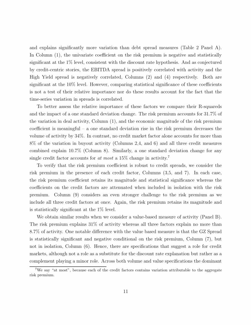
Figure 2 illustrates the fluctuations in our buyout activity measures. Following the initial
boom of the late 1980s with 20-30 deals a quarter (approximately 50bps of activity), the
1990s experienced a dearth of activity with less than 5 deals per quarter (10bps). Two
spikes in activity occurred in the following years, one in the 1997-2000 period, and another
around 2005-2007. Following the financial crisis of 2008 and a halt in activity, 2010 saw
2A key reason enterprise value averages less than book assets is that enterprise values are less consistentlyreported than asset values.
7

Figure 2: Time-Series of Buyout Activity Measures
0
5
10
Val
ue M
easu
re
0
10
20
30
40
50
Vol
ume
Mea
sure
1985q1 1990q1 1995q1 2000q1 2005q1 2010q1
Quarter
Volume Sharelog(Asset)
Figure 2 illustrates time-series variation in buyout activity. The volume-based measure is quarterly dealvolume as a percent of public firms (in bps). The value-based measure is the log of target assets (in 2010millions of dollars).
a modest rebound. These variations in number of deals are concomitant to variation in
the value of deals; our two measures have a correlation of 74%. The average log value of
activity is 8.3 or $4.1bn dollars. Value varies between 7.0 ($1.1bn) in the 25th percentile to
9.2 ($9.5bn) in the 75th percentile. While not the focus of our study, other dimensions of
the buyout transaction appear to experience cyclical variation. For instance, Axelson et al.
(2013) document variation in the composition of financing, albeit more modest. In their
sample the ratio of debt to enterprise value varies between 61% and 78% between the 25th
and 75th percentile. They also show deals originating in a boom experience lower subsequent
returns than those originating in periods of low activity. We revisit these quantities and their
relation to our main hypothesis in Section 3.
8

2.2.2 Capital market conditions
Aggregate risk premium. We measure the aggregate risk premium using an estimate
of expected excess equity returns. We utilize three factors that have been shown to pre-
dict excess returns: the dividend-price ratio, cay, and the three-month T-bill yield.3 The
dividend-price ratio is constructed using CRSP data on monthly returns. cay is an empiri-
cal proxy for the log consumption-wealth ratio.4 Interest rates are constant maturity rates
according to the Federal Reserve’s H.15 release.
The predictive regression is estimated quarterly from 1954Q1 to 2010Q3. The dependent
variable is the annualized return of the value-weighted market portfolio over the next three
years (ReM,t+1) in excess of the current three-month T-bill yield. We use a three-year window
to capture the longer-term nature of private equity investments. The regression yields the
following coefficients,
E(ReM,t+1) = −.76 + (2.89)
[1.03]
(D/P )t + (2.54)[0.59]
cayt + (−0.97)[0.38]
(T-Bill)t. (1)
For the buyout sample period, we calculate the predicted market return as a measure of
the risk premium in the economy, rpOLS. This is a projection of equity returns on predictive
factors; therefore, information in equity markets must explain the behavior of the predicted
variable.
Credit market conditions. We compare the explanatory power of our aggregate mea-
sure of risk premium with several credit market factors other researchers have emphasized as
important to explaining buyout activity. Axelson et al. (2013) find the yield on the Merrill
Lynch High Yield Index less LIBOR is correlated with leveraged buyout, EV/EBITDA ratios
and leverage. Using a composite of Merrill Lynch high-yield bond indices, we construct a
similar measure less the yield on the three-month T-bill (HY Spread). Kaplan and Stromberg
(2009) suggest firms’ ability to finance profitably with high-yield debt is an important de-
terminant of activity. We construct their proposed measure, EBITDA Spread, which is the
median EV/EBITDA ratio for COMPUSTAT firms less the yield on our composite high
3D/P : Campbell and Shiller (1988b), Fama and French (1988), Cochrane (2008); cay: Lettau andLudvigson (2001); Term structure of interest rates: Campbell (1987), Fama and French (1989).
4cay is constructed as in Lettau and Ludvigson (2001) and we download the data from Martin Lettau’swebsite (http://faculty.haas.berkeley.edu/lettau/data_cay.html)
9
yield bond index. We also consider a measure of the excess premium in corporate bonds(GZ
Spread) shown to predict future macroeconomic activity (Gilchrist and Zakrajsek, 2012).
Statistics for these variables are summarized in Table 1.
Not surprisingly, these measures are correlated with the equity risk premium, rpOLS.
HY Spread has a positive correlation with the risk premium of 55%, because an aggregate
discount factor is reflected in both debt and equity markets. This observation is consistent
with evidence that the same factors price excess returns for both stocks and bonds, e.g.
Fama and French (1993). Given this correlation, EBITDA Spread is negatively correlated
with the risk premium (-36%). Finally, the GZ Spread is also negatively correlated with our
risk premium measure, (-32%), though it is positively correlated with the spread on the high
yield index.5
2.3 Risk premium or credit factors?
Figure 1 illustrates the negative covariation between buyout activity and the risk premium
over time. The decline in activity in the early 1990s corresponds to a high risk premium
while the spikes in activity around 2000 and 2007 correspond to periods of lower expected
returns. The modest rebound in volume in 2010 also matches a subsiding risk premium. The
one boom that does not correspond as cleanly is the late 1980s.
In order to assess the importance of capital market factors, we compare the statistical
significance and explanatory power of the risk premium versus that of credit market variables.
We estimate the relation between activity and discount rates using OLS, where activity is
either the volume or value-based measure.
Activityt = α+ λrprpt + γ′(Credit Factors)t + ut
We include quarterly dummy variables to account for seasonality. Given the persistence of
independent variables, we estimate Newey-West standard errors lagged for the prior four
quarters.6
The risk premium measure is negatively correlated with the volume of buyout activity
5Correlations are detailed in Supplementary Appendix Table 12.6Technically the sample is censored at zero, though this only binds once in 1993. The coefficient estimates
are quantitatively similar in a Tobit specification; however, this limits the ability to make straightforwardR-squared comparisons.
10
and explains significantly more variation than debt spread measures (Table 2 Panel A).
In Column (1), the univariate coefficient on the risk premium is negative and statistically
significant at the 1% level, consistent with the discount rate hypothesis. And as conjectured
by credit-centric stories, the EBITDA spread is positively correlated with activity and the
High Yield spread is negatively correlated, Columns (2) and (4) respectively. Both are
significant at the 10% level. However, comparing statistical significance of these coefficients
is not a test of their relative importance nor do these results account for the fact that the
time-series variation in spreads is correlated.
To better assess the relative importance of these factors we compare their R-squareds
and the impact of a one standard deviation change. The risk premium accounts for 31.7% of
the variation in deal activity, Column (1), and the economic magnitude of the risk premium
coefficient is meaningful – a one standard deviation rise in the risk premium decreases the
volume of activity by 34%. In contrast, no credit market factor alone accounts for more than
8% of the variation in buyout activity (Columns 2,4, and 6) and all three credit measures
combined explain 10.7% (Column 8). Similarly, a one standard deviation change for any
single credit factor accounts for at most a 15% change in activity.7
To verify that the risk premium coefficient is robust to credit spreads, we consider the
risk premium in the presence of each credit factor, Columns (3,5, and 7). In each case,
the risk premium coefficient retains its magnitude and statistical significance whereas the
coefficients on the credit factors are attenuated when included in isolation with the risk
premium. Column (9) considers an even stronger challenge to the risk premium as we
include all three credit factors at once. Again, the risk premium retains its magnitude and
is statistically significant at the 1% level.
We obtain similar results when we consider a value-based measure of activity (Panel B).
The risk premium explains 31% of activity whereas all three factors explain no more than
8.7% of activity. One notable difference with the value based measure is that the GZ Spread
is statistically significant and negative conditional on the risk premium, Column (7), but
not in isolation, Column (6). Hence, there are specifications that suggest a role for credit
markets, although not a role as a substitute for the discount rate explanation but rather as a
complement playing a minor role. Across both volume and value specifications the dominant
7We say “at most”, because each of the credit factors contains variation attributable to the aggregaterisk premium.
11
factor in buyout activity is the risk premium: the risk premium measure explains 2.5 to 10
times the variation that credit factors explain, the risk premium is negative and statistically
significant, and the estimates of the risk premium coefficient are robust to the inclusion of
credit measures as controls.
We find a similarly significant coefficient on the risk premium in the early buyout waves
of 1982-1991 as in the later waves, 1992-2014. However, the R-squared is lower in the earlier
period (16%) versus the later period (54%). The lower explanatory power in the 1980s
is consistent with an initial burst in activity facilitated by the development of the buyout
investment technology (Figure 1).
We use another method to link buyout activity and the risk premium. If buyout decisions
do indeed reflect agents’ expectations about the level of the risk premium, then buyout
activity should predict future stock returns. A monthly regression of annualized excess
returns for the next three years on the volume measure of buyout activity from July 1982 to
September 2010 yields,8
ReM,t+1 = 10.52 + (−0.65)
[0.28]
(V olume%t) + εt+1. (2)
demonstrating that buyout activity has statistically significant predictive power on long term
stock market returns.
Robustness. These conclusions are robust to other measures of buyout activity, additional
credit metrics, and alternative estimates for the risk premium. Supplementary Appendix
Table 13 considers six different measures of buyout activity. The first three are alternative
value measures: the log of enterprise value in a quarter, the log of buyout assets to total public
assets, and the log share of buyout enterprise value to total public enterprise value. The next
three are measures of activity based on a matched sample to account for time-variation in
firm composition. For example, if potential buyout targets vary over time then our results
may proxy for changes in firm type. For each measure, we compare the explanatory power
of the risk premium to that of the three credit factors. We also consider the risk premium
in the presence of all three factors to see if the credit variables attenuate the role of the
8The standard errors are Newey-West with autocorrelation over the prior 36 months and the R-squaredis 0.11.
12

risk premium. Across all of these measure of buyout activity the explanatory power of the
risk premium is 1.5-5x that of the credit factors. In addition, the magnitude and statistical
significance of the risk premium is not diminished by the inclusion of credit variables.
We focus our analysis on public-to-private buyout activity for several reasons: there is
more information about transactions with public targets, it is possible to consider a counter-
factual set of similar firms, and the change in funding is particularly dramatic from public-
to-private. Nevertheless, the discount rate may play a role in private-to-private buyout
transactions as well. In Supplementary Appendix Table 14 we repeat the analysis of Table
2 using the private-to-private buyout volume from Thomson SDC. Again, the risk premium
explains more variation than credit factors and is robust to their inclusion; however, it is
difficult to directly compare these results with public-to-private activity because we have no
way of controlling for the set of potential targets.
We also find that our results are robust to alternative estimates of the risk premium,
Supplementary Appendix Table 15. We estimate three alternative measures: a rolling mea-
sure that eliminates look-ahead bias, a measure that excludes the T-bill yield as a factor
to eliminate any form of credit predictor, and a risk premium estimate that assumes per-
fect foresight by using actual future excess returns on the market portfolio. We test these
alternative risk premia for both the volume and value measures of activity. In five of the
six specifications the risk premium R-squared exceeds the credit factor alone. In six of six
specifications the risk premium coefficient is robust to the inclusion of credit factors.
For the volume measure of activity, Panel A, the risk premia R-squareds vary from a low
of 16.6% on the rolling risk premium and actual returns to a high of 23.7% on the measure
excluding the T-bill, Columns (1), (5) and (3) respectively. Albeit lower in explanatory power
than our composite measure, they are in excess of the 10.7% credit factors achieve (Table 2
Panel A, Column 8) and they are robust to including credit factors in the regression, Columns
(2), (4), and (6). For the value measure of activity, the R-squareds range from 11.3% on the
actual return (Column 5) to 23.2% using the measure excluding the T-Bill (Column 3). Two
of the three specifications exceed the explanatory power of the three credit factors (13.8%).
All three risk premium measures are significant in the presence of credit factors.
Finally, we explore additional credit metrics, Supplementary Appendix Table 16, includ-
ing the corporate bond spread, aggregate market leverage, book leverage, and the change in
credit standards as measured by the Federal Reserve Senior Loan Officer Survey. For both
13

volume and value based measures of activity, the risk premium accounts for a sizable portion
of the variation and the R-squared is well in excess of the credit metrics. Again, the role of
the risk premium is not mitigated by the inclusion of alternative credit metrics.
2.4 The three fundamental components of valuation
Our central argument is that aggregate changes in the valuation environment affect the deci-
sion to enter a buyout. Thus far we have focused our analysis on the most important driver
of prices, the risk premium; however, it is not the only component of valuation. Following
Campbell and Shiller (1988a) and subsequent work, we decompose aggregate valuations be-
tween expected future returns and expected future earnings growth. Further, we separate
expected future returns between the risk premium and a risk-free component. We then study
how fluctuations in buyout activity can be ascribed to these three distinct components.
We follow the standard approach of representing the joint dynamics of these quantities by
a vector autoregression (VAR), which results in a simple representation of expectations. We
include the same variables as Campbell and Ammer (1993), augmented by cay of Lettau and
Ludvigson (2001).9 We estimate the dynamics of the VAR on a long sample from 1972Q1 to
2012Q4. We extract a time series forecast for two components: stock market excess return
rpV AR and earnings growth g, for the next three years. For the third component, the risk-free
rate, we directly observe the three-year Treasury yield.10
For each component we construct annualized rates; Table 3 contains a summary of the
resulting estimates. The predicted risk premium from the VAR is remarkably similar to
our OLS measure with a correlation coefficient of 0.89. Future earnings growth is also
positively correlated with the OLS measure. A potential concern for time series analysis
is the persistence of the three variables. While the quarterly autocorrelation of the risk
premium and earnings growth are below 0.4, that of the risk-free rate is 0.96. This high
persistence hinders our ability to draw strong inferences about the role of the risk-free rate.
Consistent with valuation predictions, buyout activity is negatively related with the risk
9Our VAR specification includes the following 7 variables: excess returns, risk-free rate, earnings growth,
dividend-price ratio, cay, the change in the 3-month yield y(3m)t − y
(3m)t−1 , the slope between the 10 year and
one month yield y(10y)t − y
(1m)t , and the one-month yield minus its moving average over the previous 12
months y(1m)t − 1/12
∑t−1τ=t−12 y
(1m)τ .
10Constant maturity three-year yields are obtained from the Federal Reserve Board FRB H.15 release.
14
premium component and positively related with expected earnings growth for both the
volume and value of activity, Table 4. Columns (1) and (4) consider the VAR risk premium
alone and find coefficients of similar magnitude as our OLS estimates in the prior section.
In addition the explanatory power exceeds that of the credit factors by at least 1.5x (see
Table 2). We add expected earnings growth to the specification and find a positive and
statistically significant relation between buyout activity and earnings growth, Columns (2)
and (5). The impact of earnings growth is smaller than that of the risk premium. A one
standard deviation change in expected growth has approximately half the impact of a similar
change in risk premium (17-25% for volume, 6-9% for value).
The risk-free rate estimates are more difficult to interpret. The risk-free yield is positive
but statistically indistinguishable from zero for volume (3) and positive for value (7). A
simple discount rate argument would predict a negative relation with activity. As discussed
earlier, the persistence of the risk-free rate makes statistical inference unreliable. In addition,
if the risk-free rate proxies for economic conditions it further complicates interpretation (e.g.
Stock and Watson (1999) show that periods of high risk-free rates coincide with economic
growth). Augmenting these factors with the credit measures in Columns (4) and (8) does
little to alter the estimated coefficients.
Robustness. We consider several alternative proxies for market expectations in Table 5
and examine their relation with the volume of buyout activity. For each set of alternative
forecasts, we estimate the role of the forecasts alone and then in the presence of credit market
controls. These two specifications give us the explanatory power of the forecasts and the
robustness of the coefficients to the presence of credit controls.
The first specification is based on a VAR using dividends rather than earnings. The
dividend VAR, Columns (1) and (2), results in qualitatively similar estimates to those in
Table 4. The salient difference is that while the coefficient on dividend growth is positive, it
is not statistically significant.
We also consider several non-VAR measures of the market’s expectations. Thomson IBES
provides S&P earnings estimates based on a survey of equity analysts. Using the average
from the survey, we construct the annual growth rate over the next two years to serve as a
proxy for expected growth. The survey-based growth measure, in tandem with the OLS risk
premium from 2.3, results in similar coefficients to prior specifications and an R-squared of
15
37.4%, (3) and (4).
In Columns (5)-(8), we assume perfect foresight and replace forecasts and surveys with
realized future growth and equity returns. For growth we aggregate EBIT for the sample of
COMPUSTAT firms and calculate one-year forward growth rates. We choose EBIT growth
in order to focus on a measure of growth that is independent of capital structure, though
we obtain similar results using realized net income growth. In (5) and (6) we use the actual
forward EBIT growth and the OLS risk premium prediction. Both specifications resemble
prior estimates, with an R-squared of 38.8%, a coefficient on the risk premium of -1.17, a
coefficient on EBIT growth of 0.25 and a coefficient on the risk-free rate of 0.75 (statistically
insignificant). In the final two columns we use EBIT growth and realized future equity
returns rather than predicted equity returns. The risk premium coefficient and R-squared
estimates are lower at -0.52 and 24.8%, respectively; however, this is not surprising given
the additional noise in realized returns.
The message is consistent across specifications: the aggregate risk premium is the largest
explanatory factor, expected growth enters positively, and the risk-free rate is generally
positive but frequently indistinguishable from zero. The evidence in this section strongly
suggests the risk premium is the most important driver of buyout activity. To further
test this explanation against alternative hypotheses, we articulate a parsimonious theory
of the buyout decision which provides a clear rationale for the role of aggregate valuation
conditions.
3 A simple model of the buyout transaction
We develop a two-period model that relates the buyout decision to the aggregate risk pre-
mium. Our theory relies on two key intuitions. First, performance improvements generated
by buyout deals are valued using a Net Present Value (NPV) rule.11 When the risk premium
is large, the cost of capital lowers valuations and fewer projects are undertaken. Second,
because of an agency problem, the general partner (GP) has to bear excess risk to be duly
motivated to implement changes in the firm. When the risk premium increases, i.e. when
the marginal willingness to bear risk decreases, the willingness to bear this excess risk also
11The private equity industry explicitly incorporates an NPV rule by relying on Discounted Cash Flowmodels to assess potential investments.
16

decreases and compensating the GP becomes more costly.
The model not only provides a precise rationale for the results in Section 2, but also
allows us to make additional empirical predictions. We rationalize both the positive corre-
lation between buyout activity and deal leverage, as well as the positive correlation between
pricing and subsequent returns. Moreover, we develop further insights on the changing char-
acteristics of buyout targets as the risk premium fluctuates, providing additional predictions
we test in Section 4.
3.1 Setup
There are two periods. At time 0, an acquirer, the GP hereafter, considers a firm, the target,
for a buyout deal. The target’s output is realized at time 1 and is unknown as of 0. The
following describes the distribution of firm output,
Y = µ+ βεm + εi,
where µ is the average output, εm is an aggregate shock and εi is an idiosyncratic shock.
The shock variables are independent from each other, normally distributed with mean 0 and
variances σ2m and σ2
i respectively. The loading β captures the target’s exposure to systematic
risk. The target’s outcome at time t = 1 is contingent upon the GP’s actions:
1. If she decides not to acquire the target, output is Y .
2. If she implements a buyout deal and improves management of the target, output is
pH Y with pH > 1.
3. If she implements the deal without improving management, output is pLY , with ∆p =
pH − pL > 0. She receives a private benefit linear in output: bY .
The GP must find a contractual arrangement with outside investors, i.e. financial mar-
kets, to finance the deal. We assume the GP’s action is not directly contractible. Therefore
an agency friction is present: without a stake in the firm, the GP does not implement
managerial changes and instead chooses to collect her private benefit. We now introduce
assumptions about how those agents make decisions.
Preferences of the GP. The GP has initial wealth W0. She can invest on public markets
or engage in a buyout. She has constant absolute risk aversion (CARA) preferences over
17

consumption with risk aversion γ: −E[− exp(−γC)]. If consumption is normally distributed,
this utility function corresponds to a mean-variance evaluation, U = E[C]− γ2var[C].
Cost of capital on public markets. We assume no-arbitrage on financial markets, hence
there is a stochastic discount factor. We also assume the stochastic discount factor solely
loads on the aggregate risk factor, εm, and the risk premium for exposure to the market is
Rem = E0[R
em] which is proportional to the market risk σ2
m.12 Risk-free claims are discounted
at the rate 1 + rf . Therefore, the cost of capital is determined by the Capital Asset Pricing
Model (CAPM). For instance, the price of a payoff 1 + βεm + εi is NPV(1 + βεm + εi) =
(1− βRem)/(1 + rf). We detail the equivalence to a standard Discounted Cash-Flow (DCF)
analysis in Appendix A.1. Current owners of the target and outside investors value their
claims using this cost of capital because these claims are traded on competitive markets.
3.2 Solution
A buyout of the target occurs if the GP and outside investors find an arrangement that is
valuable to both. To find whether such contracts exist, we first derive the minimum cost of
providing incentives to the GP, then we verify if the net returns to outside investors of the
buyout deal are positive under such an arrangement
GP’s outside option. If the GP does not engage in the buyout, she invests her wealth
on public markets. Without loss of generality, she chooses her portfolio investment between
the risk-free rate (θ0), a zero-cost portfolio that pays off the market excess return (θm) and
a zero-cost portfolio that loads on idiosyncratic risk (θi). Given her absolute risk aversion γ,
her utility is:
Uoutside = max(θ0,θm,θi)
θ0 + θmRem −
γ
2(θ2mσ
2m + θ2i σ
2).
Her budget constraint is θ0 ·1
1+rf+ θm · 0 + θi · 0 ≤ W0, which gives θ∗0. Her position in the
market is determined by the price of market risk and her risk aversion, θ∗m = Rem/(γσ
2m).
12These assumptions arise exactly if we assume buyout transactions constitute an infinitesimal part of aneconomy where total output is exposed to εm and all investors have CARA preferences. Investors may haveheterogeneous risk aversion that is, in particular, different from the GP. While we focus on variation in riskpremium driven by changes in aggregate risk, all of our predictions also hold for a change in risk premiumin response to a proportional change in risk aversion in the economy. In other words we are agnostic as tothe source of variation in risk premium: quantity or price of risk.
18

Idiosyncratic risk is not compensated by a risk premium, hence her optimal allocation is
zero, θ∗i = 0. Given our assumptions about pricing, the investments in the outside option do
not depend on market conditions.
Cost of incentives. The GP will only invest in the deal and implement productive changes
if she is adequately incentivized to do so. Outside investors must design a contract such
that the GP implements changes that exceed the value of private benefits – the incentive
compatibility constraint (IC). The contract must also incentivize the GP to partake in the
buyout deal rather than invest in her outside option, i.e. the individual rationality constraint
(IR).
For simplicity we restrict ourselves to linear contracts. A contract features a fixed compo-
nent k0 and a variable part proportional to the target’s output with coefficient k1 controlling
its riskiness. Outside investors minimize the cost of providing incentives to the GP, the
agent.13 To find the cheapest contract, outside investors solve:
min{k0,k1}
NPV(k0 + k1pH Y )−W0
= min{k0,k1}
(k0 + k1pH(µ− βRe
m))/(1 + rf)−W0,
under the IC and IR constraints
U(k0 + k1pH Y ) ≥ U(k0 + k1pLY + bY ) (IC),
U(k0 + k1pH Y ) ≥ Uoutside (IR).
The IC constraint reduces to a lower bound on the slope of the incentive contract, k1 ≥
b/∆p. Indeed the GP must have a large enough stake in the firm so that her returns from
exerting action pH rather than pL dominate her private benefit of not implementing the
changes b.
To understand the IR constraint it is helpful to represent the payoff as an equivalent
13For most of our analysis we consider whether feasible deals exist, so bargaining power or the surplussharing rule is irrelevant.
19
portfolio invested in the risk-free asset, market excess return, and idiosyncratic risk:
θ0 = k0 + k1pH(µ− βRem)
θm = k1pHβ
θi = k1pH .
(3)
Recall the utility is linear in θ0 and quadratic in the two risky components θm and θi. Hence
the IR constraint is equivalent to the difference with the optimal portfolio θ∗:14
θ0 − θ∗0 ≥1
2Re
m
1
θ∗m(θm − θ∗m)
2 +1
2γσ2
i θ2i .
Under this form, the left-hand side of the constraint coincides with the objective function
and the right-hand side with the cost for the GP of bearing risk that deviates from her
outside option.
We can now solve for the optimal contract. If, to have incentives to properly manage the
firm, the agent must receive excessive amounts of risk relative to her outside option, which
we assume, increasing k1 tightens the right-hand-side.15 Hence the principal minimizes the
slope of the contract such that the IC constraint binds: k∗1 = b/∆p. To find the optimal
level, we find the lowest fixed payment k0 that satisfies the IR constraint:
k∗0 + k∗
1pH(µ− βRem)−W0(1 + rf ) =
1
2Re
m
1
θ∗m(k∗
1pHβ − θ∗m)2 +
1
2γσ2
i k∗21 p2H .
3.3 When do deals occur?
Proposition 1. A buyout deal occurs if it yields positive returns net of the GP’s compensa-
tion. This translates into the following condition:
14We are using the observation that if f(x) = ax2+bx+c with extremum reached at x∗, then f(x)−f(x∗) =a(x− x∗)2.
15Formally, the condition is σ2mpHβ(k1pHβ − θ∗m) + σ2
i k1 > 0 at k1 = b/∆p. Two different sufficientconditions for this relation to hold are that the agent bears excessive amounts of aggregate risk, k1pHβ > θ∗m,or that idiosyncratic risk is large relative to aggregate risk, σ2
i ≫ σ2m. Both assumptions are likely to hold
empirically; we discuss the first one more precisely later in this section.
20

(pH − 1)(µ− βRe
m
)
︸ ︷︷ ︸
Performance Channel
≥1
2Re
m
1
θ∗m(k∗
1pHβ − θ∗m)2 +
1
2γσ2
i k∗21 p2H
︸ ︷︷ ︸
Illiquidity Channel
(4)
The deal surplus is:
1. decreasing in expected market return Rem (via the performance and illiquidity channel)
2. decreasing in the market risk exposure β (via the performance and illiquidity channel
if k∗1pHβ > θ∗m).
16
3. decreasing in idiosyncratic volatility (via the illiquidity channel).
Performance channel. The left-hand side of condition (4) is the performance channel. It
corresponds to the net value of the cash-flow gains from improving management. In periods
of high risk premium, those cash-flows are discounted more, and this value is lower, which
decreases the likelihood of a deal.
Illiquidity channel. The right-hand side of (4) is the illiquidity channel.17 It is the
monetary cost of compensating the GP for taking excessive amounts of risk relative to her
outside option. The cost of this deviation is larger when the risk premium is larger. Indeed,
the equilibrium risk premium corresponds to the marginal cost of bearing risk. Similarly, the
illiquidity cost is the total cost of deviating from the optimum, also driven by the convexity
in the utility function — here determined by γ — and the risk facing the investor. In other
words, periods where investors do not want to bear risk at the margin correspond to periods
where investors ask a large compensation for bearing excessive risks.
The main restriction we imposed on the contracting space is the absence of benchmarking
to the market. While in practice buyout contracts are not benchmarked, we consider the
impact of relaxing this assumption in Appendix A.2. Clearly, this change has no impact
on the performance channel. If the market exposure β is known at the time contracting,
16In other words, the illiquidity channel is impacted by market exposure if the GP has to bear moreaggregate risk than in her outside option. If we assume that her outside option is entirely invested in theequity market, and the leverage is 70% post-buyout and 35% pre-buyout (consistent with the evidence inAxelson et al. (2013)), then this condition holds as long as the pre-buyout equity β is larger than 0.5, whichholds for most firms.
17We use the term illiquidity to signify the inability to trade out of a position. In our framework, illiquidityarises as a contractual solution to the agency problem. It differs from the inability to find a buyer on shortnotice in the case of an adverse shock.
21

then the contract brings the GP back to her optimal loading on aggregate risk. However,
in the more realistic case where the target’s β is not known at the time of contracting, we
show the GP always ends up with an inappropriate amount of aggregate risk, maintaining
an illiquidity cost increasing in the risk premium.18
3.4 Predictions
Changes in aggregate conditions affect the surplus of each potential deal; therefore, we are
able to derive several empirical predictions related to the aggregate facts documented in
Section 2. We also focus on how particular firms are impacted by aggregate conditions.
Prediction 1. Buyout activity is larger in times of low risk premium.
The role of the risk premium is driven by both the performance and illiquidity channels.
Table 4 confirms this prediction and shows a significant negative impact of the risk premium.
The impact of the aggregate risk premium on the illiquidity compensation, combined with
its contribution to the performance channel, rationalizes the observed sensitivity of buyout
activity to the risk premium.
The model yields additional predictions about the composition of buyout waves. We
show firms’ risk characteristics impact their likelihood of being a deal target.
Prediction 2. A firm is more likely to be in a buyout if it has (1) low market beta, or
(2) low idiosyncratic risk.
The negative impact of the market beta comes through both channels, whereas idiosyn-
cratic risk only affects the illiquidity channel. The distinct roles of the systematic and
idiosyncratic risk of a firm are a novel prediction of our model.
Beyond their unconditional impact, risk characteristics interact with aggregate condi-
tions. Changes in the risk premium affect not only the quantity but also the composition of
buyouts.
18Ewens et al. (2013) also assumes the target’s characteristics are unknown at the time of contracting.However they find empirical support for this assumption studying the role of idiosyncratic risk. We drawnovel implications for the role of the risk premium.
22
Prediction 3. Over time, (1) firms with high market beta are more sensitive to fluctuations
in the risk premium, and (2) firms with large potential performance gains (high pH) are more
sensitive to the risk premium.
The first interaction comes from both channels, whereas the second is due to the perfor-
mance channel alone. Interestingly, such a result is not present for idiosyncratic risk. This
difference allows us to distinguish our approach from an explanation of buyout waves related
to changes in debt capacity. Section 4.3 considers the role of risk characteristics in the data,
and Section 4.4 examines the changing composition of buyouts.
The structure of outside financing between debt and equity is not pinned down in our
theory: all capital is provided at the public markets’ cost of capital. However, a natural
way to implement outside financing is to split between an equity claim proportional to the
GP’s payoff and a safer debt claim.19 In this case, leverage is determined by the slope of
the contract k∗1. To understand variations in leverage, we extend the model in Appendix
A.3 to allow for heterogeneity across targets. The optimal level of leverage k∗1 varies with
the parameters. A higher private benefit relative to the impact on the firm requires a more
highly levered position to incentivize effort. However, higher leverage is costly because of
the increased illiquidity costs. High-leverage deals are only feasible when it is relatively
cheap to compensate the acquirer for her levered position, i.e. when the risk premium is low.
Therefore, our framework predicts that the leverage of the average buyout is higher in times
of low risk premium and high deal activity.
Prediction 4 (Leverage). Buyouts are more levered in times of low risk premium.
Axelson et al. (2013) study fluctuations in buyout leverage concomitant with variations in
mispricing measures. More generally, they find leverage covaries positively with fluctuations
in aggregate buyout activity. The prediction demonstrates this result can be explained in a
model in which there is no notion of mispricing between debt and equity.
The model implies that pricing of targets and performance of private equity investments
vary over the buyout cycle. All investors, controlling and non-controlling, receive the stan-
19Such an approach is similar to Axelson et al. (2009) who focus on a particular contractual implementationin an environment where outside capital is also provided at an exogenous cost irrespective of debt and equity.
23

dard compensation for risk on public markets which is larger when the risk premium is high.
The GP receives additional compensation for her excess risk, which also positively varies
with the risk premium. These variations in returns are reflected in the transaction price:
higher future returns are related to a lower transaction price.
Prediction 5 (Returns and deal pricing). (1) When the risk premium is low, outside in-
vestors and the acquirer receive lower expected returns on their private equity investments.
(2) The acquirer receives positive abnormal returns after adjusting for the market pricing of
risk, and those abnormal returns are larger in times of high risk premium. (3) When the
risk premium is low, the transaction price is high.
The recent literature on private equity returns largely confirms these inferences (Kaplan
and Schoar (2005), Robinson and Sensoy (2013a), Harris et al. (2014)). Buyout fund re-
turns exhibit cyclical patterns consistent with our first prediction; investments in “hot” deal
markets suffer from lower returns. Moreover, these findings are in direct contradiction with
a credit market view where buyout investors are optimally timing credit market conditions
to obtain high returns in booms, as pointed out by Axelson et al. (2013). Given the GPs
receive fees and carried interest in addition to their ownership stake, their returns will be
higher on average and covary with the fund (e.g. Metrick and Yasuda (2010), Robinson and
Sensoy (2013b)). On deal pricing, Axelson et al. (2013) document higher valuation ratios
(EV/EBITDA) for buyout deals in periods of high activity.
4 The composition of buyout activity
Our theory provides a precise rationale for the link between the risk premium and buyout
activity. It also delivers insights into the types of firms targeted by buyout investors across
episodes of high and low risk premium. In this section we use a panel dataset of public firms
to document that the composition of buyout activity reflects the forces of our model. Our
results further emphasize the role of the risk premium in the buyout decision and in their
totality cannot be reconciled with alternative views of the buyout cycle.
24
4.1 Data
We construct a quarterly panel of U.S. public companies using annual accounting data from
COMPUSTAT and quarterly share price information from CRSP. As we are looking to
exploit accounting data, we exclude the financial industry as defined by the Fama-French 12
classification. Once a firm announces a buyout, they exit our sample. Bias resulting from
the exit of buyout firms is small, given the low number of deals relative to the number of
public firms. The resulting unbalanced panel of 501,176 firm-quarters tracks 14,386 unique
firms over 117 quarters and contains 1,043 deal firm-quarters, where a deal firm-quarter is
defined as the quarter of a buyout announcement.
We use this panel to consider cross-sectional predictions related to the risk character-
istics of firms. The model predicts that firms with greater volatility will be less attrac-
tive targets. We proxy for volatility using the monthly return volatility over the past two
years, σ(Re), as well as an accounting based metric, the standard deviation of EBITDA,
σ(EBITDA/Assets). The model ascribes different roles to systematic and idiosyncratic
risk. We estimate the market regression to calculate each firm’s market beta, β, and the
volatility of residuals, σ(ε), as measures of systematic and idiosyncratic risk. We unlever
these equity-based measures of risk, as the model specifies total firm risk.20 We trim the
top and bottom 1% of accounting ratios and the top and bottom 5% of market based risk
measures to reduce the impact of large outliers on our analysis.
Our theory is not meant to be comprehensive on the determinants of what makes a
good buyout in the cross-section. Rather, our model focuses on the elements of a deal
that relate to risk and discount rates. Therefore, we consider several firm characteristics
that Opler and Titman (1993), and more recently Bharath and Dittmar (2010), identify
as empirically important to explaining which types of firms are bought out or go-private:
cash-flow (EBITDA/Assets), capital intensity (CapEx/Sales), costs of financial distress
(R&D/Sales), liquidity (Turnover), payout policy (Dividend Dummy), and net leverage
(Net Debt/Assets).21 In addition we control for firm size (log(Assets)). Table 6 summarizes
the characteristics of our sample. The broad picture is consistent with prior findings in the
20Both β and σ(ε) are unlevered by rescaling by 11+(1−τ)∗ Debt
Mkt Cap
where we assume τ = 35%.21We also note the book-to-market of firms, although this is not a factor in our analysis, as it is a pricing
factor. In unreported results we find our conclusions are robust to this additional control, but this is not ourpreferred specification.
25
literature: deal firms are more profitable, spend less on capital expenditures and research
and development, are less liquid and have higher net debt than the average public firm.
A comparison of deal firm-quarters to the full panel of firm-quarters demonstrate that the
average buyout has lower risk across the set of risk proxies.
4.2 The role of aggregate factors
Before analyzing cross-sectional heterogeneity in buyout propensity, we revisit the role of
aggregate factors. The panel specification allows us to explicitly control for changes in firm
composition. We cannot observe the surplus from going private, but the likelihood of a
firm being a target is increasing in the difference between their private and public valuation.
We use a dummy variable equal to one for the firm-quarter of a deal announcement and
estimate the likelihood of a firm going private via OLS conditional on the risk premium and
credit-market conditions at the beginning of the quarter.
Dealit = αi + λrprpt + γ′(Credit Factors)t + ǫit. (5)
Firm fixed effects capture the heterogeneity across firms. Standard errors are clustered in
two dimensions, by firm and quarter, and robust to arbitrary serial correlation within a
bandwidth of one year.22
The panel introduces significant additional variation to the exercise; we are not only pre-
dicting when deals occur, but we are also predicting which firms are targeted. Consequently,
R-squared comparisons are not all that informative, but we can verify the sign, statistical
significance, and robustness of the discount rate measures conditional on firm-level controls.
Consistent with the aggregate results of Section 2, Table 7 demonstrates that a higher risk
premium lowers the probability of a deal even in the presence of credit controls and firm
fixed effects. This result is true for both the reduced form risk premium, rpOLS in Columns
(1) and (9), and the VAR estimates, (10) and (11). The latter also demonstrates a positive
relation between earnings growth and deal likelihood. The risk premium and growth rate
results are consistent with Prediction 1. In contrast to the aggregate tests, the risk-free
rate is negatively correlated in this specification and statistically significant. However, we
22The estimator is intended to account for autocorrelation in common disturbances (like changes in therisk premium) across the panel.
26

reiterate that the risk-free rate coefficients are unreliable because the risk-free rate is highly
persistent.
When we consider specific credit market factors we find both the EBITDA spread and
the high yield spread are statistically significant in isolation, Columns (2) and (4), but
statistically indistinguishable from zero when regressed in conjunction with the risk premium,
(3) and (5). The GZ Spread is positive and statistically significant at the 1% level in both
specifications, but does not attenuate the risk premium. The positive correlation (the higher
the risk premium in bonds the more buyout activity) is not consistent with the aggregate
results in Table 4 nor is it easily reconciled with a simple credit story of buyout activity. We
confirm these results in a Probit specification (Supplementary Appendix Table 17).23
4.3 The role of risk characteristics
The remaining columns of Table 8 consider the role of risk characteristics in the cross-section
of firms. According to our framework, riskier firms are relatively more costly to acquirers
and therefore less likely to be targeted. Greater systematic risk decreases the surplus via
both the performance and illiquidity channels, while idiosyncratic risk increases the cost of
a deal to private investors via the illiquidity channel. We estimate the likelihood of a firm
going private via OLS conditional on firm risk factors and controls,
Dealit = α+ λββit + λσσ(ε)it + γ′Controlsit + ǫit. (6)
The risk characteristics exhibit time-variation, and this variation may be correlated with
other factors, particularly discount rates. Therefore, we include time fixed effects to focus the
analysis on cross-sectional differences between firms rather than time-series differences in firm
risk estimates. We also consider specifications that control for firm-level characteristics using
industry fixed effects and the firm variables discussed earlier (cash-flow, capital intensity,
etc.). Standard errors are clustered in two dimensions, by firm and quarter, and robust to
arbitrary serial correlation within a bandwidth of one year.
Congruent with Prediction 2, several proxies for risk are negatively correlated with deal
likelihood, as shown in Table 8. Columns (1)-(3) include quarter fixed effects and (4)-(6)
include firm-level controls. Both stock return volatility and cash-flow volatility decrease the
23The one exception is that the risk-free rate is positive in the Probit specification.
27
likelihood of a deal, (1) and (2), even when controlling for other factors, (4) and (5), at the
1% significance level. Market beta and idiosyncratic risk decrease the likelihood of a deal in
both specifications (3) and (6) at the 1% significance level. Again, we verify our findings in
a non-linear probability specification in Supplementary Appendix Table 18.
These results are consistent with our model. But they can also be explained by a credit-
based narrative where risk increases the probability of default thereby limiting debt capacity
and reducing the attractiveness of the firm to buyout investors. To further separate these
explanations we turn to cyclical variation in the role of firm risk and characteristics.
4.4 The composition of buyouts over the cycle
To directly test the channels outlined in the model, we consider whether the composition of
buyout firms varies with the risk premium in the manner outlined in Prediction 3. Firms
with high betas are particularly sensitive to changes in the risk premium as a decline si-
multaneously increases performance gains and lowers illiquidity costs. We go on to test
each channel independently by exploring predictions constrained to only one channel. The
performance channel predicts that firms with greater potential for improvement are more
sensitive to changes in the discount rate. The illiquidity channel predicts that more illiquid
firms should be more sensitive to the risk premium. We find empirical support for both
mechanisms.
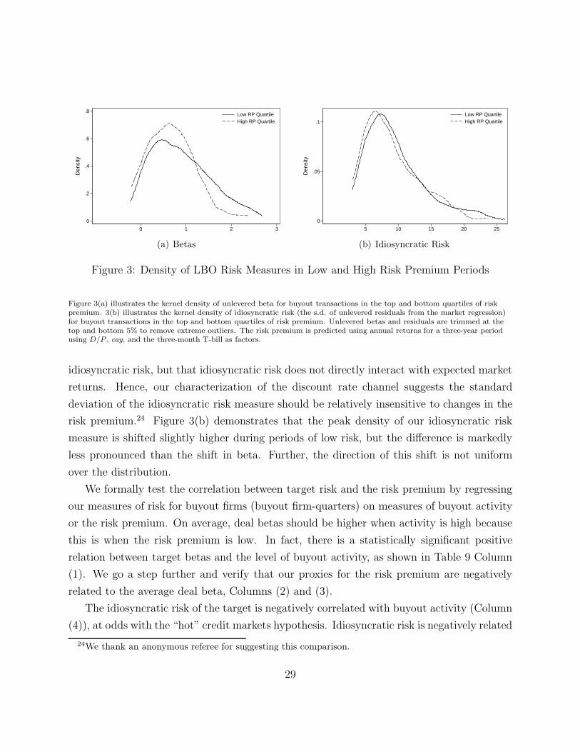
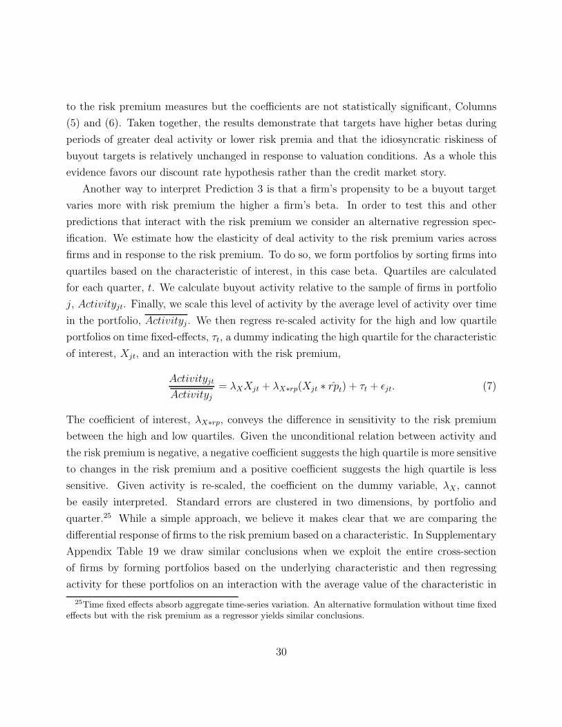
4.4.1 The riskiness of buyout targets
As the risk premium declines, firms with higher betas are more likely to satisfy the positive
surplus condition (Equation (4)). Indeed, if we compare the distribution of deal betas for
low and high quartile risk premium observations, as shown in Figure 3(a), the low quartile
distribution exhibits more mass above one, whereas the high risk premium observations are
more concentrated below one. This pattern is consistent with a rising cut-off as buyout
investors exhibit an increased willingness to purchase higher beta firms.
The sensitivity of target betas to the risk premium could also be consistent with a credit
market story in which credit investors are more willing to take risks in boom times and
less willing during busts. If “hot” credit markets drive this pattern we would expect to see
a similar shift in idiosyncratic risk. Our model predicts deals are less likely the higher the
28
0
.2
.4
.6
.8
Den
sity
0 1 2 3
Unlevered Beta
Low RP QuartileHigh RP Quartile
(a) Betas
0
.05
.1
Den
sity
5 10 15 20 25
Unlevered Residual SD
Low RP QuartileHigh RP Quartile
(b) Idiosyncratic Risk
Figure 3: Density of LBO Risk Measures in Low and High Risk Premium Periods
Figure 3(a) illustrates the kernel density of unlevered beta for buyout transactions in the top and bottom quartiles of riskpremium. 3(b) illustrates the kernel density of idiosyncratic risk (the s.d. of unlevered residuals from the market regression)for buyout transactions in the top and bottom quartiles of risk premium. Unlevered betas and residuals are trimmed at thetop and bottom 5% to remove extreme outliers. The risk premium is predicted using annual returns for a three-year periodusing D/P , cay, and the three-month T-bill as factors.
idiosyncratic risk, but that idiosyncratic risk does not directly interact with expected market
returns. Hence, our characterization of the discount rate channel suggests the standard
deviation of the idiosyncratic risk measure should be relatively insensitive to changes in the
risk premium.24 Figure 3(b) demonstrates that the peak density of our idiosyncratic risk
measure is shifted slightly higher during periods of low risk, but the difference is markedly
less pronounced than the shift in beta. Further, the direction of this shift is not uniform
over the distribution.
We formally test the correlation between target risk and the risk premium by regressing
our measures of risk for buyout firms (buyout firm-quarters) on measures of buyout activity
or the risk premium. On average, deal betas should be higher when activity is high because
this is when the risk premium is low. In fact, there is a statistically significant positive
relation between target betas and the level of buyout activity, as shown in Table 9 Column
(1). We go a step further and verify that our proxies for the risk premium are negatively
related to the average deal beta, Columns (2) and (3).
The idiosyncratic risk of the target is negatively correlated with buyout activity (Column
(4)), at odds with the “hot” credit markets hypothesis. Idiosyncratic risk is negatively related
24We thank an anonymous referee for suggesting this comparison.
29
to the risk premium measures but the coefficients are not statistically significant, Columns
(5) and (6). Taken together, the results demonstrate that targets have higher betas during
periods of greater deal activity or lower risk premia and that the idiosyncratic riskiness of
buyout targets is relatively unchanged in response to valuation conditions. As a whole this
evidence favors our discount rate hypothesis rather than the credit market story.
Another way to interpret Prediction 3 is that a firm’s propensity to be a buyout target
varies more with risk premium the higher a firm’s beta. In order to test this and other
predictions that interact with the risk premium we consider an alternative regression spec-
ification. We estimate how the elasticity of deal activity to the risk premium varies across
firms and in response to the risk premium. To do so, we form portfolios by sorting firms into
quartiles based on the characteristic of interest, in this case beta. Quartiles are calculated
for each quarter, t. We calculate buyout activity relative to the sample of firms in portfolio
j, Activityjt. Finally, we scale this level of activity by the average level of activity over time
in the portfolio, Activityj . We then regress re-scaled activity for the high and low quartile
portfolios on time fixed-effects, τt, a dummy indicating the high quartile for the characteristic
of interest, Xjt, and an interaction with the risk premium,
Activityjt
Activityj= λXXjt + λX∗rp(Xjt ∗ rpt) + τt + ǫjt. (7)
The coefficient of interest, λX∗rp, conveys the difference in sensitivity to the risk premium
between the high and low quartiles. Given the unconditional relation between activity and
the risk premium is negative, a negative coefficient suggests the high quartile is more sensitive
to changes in the risk premium and a positive coefficient suggests the high quartile is less
sensitive. Given activity is re-scaled, the coefficient on the dummy variable, λX , cannot
be easily interpreted. Standard errors are clustered in two dimensions, by portfolio and
quarter.25 While a simple approach, we believe it makes clear that we are comparing the
differential response of firms to the risk premium based on a characteristic. In Supplementary
Appendix Table 19 we draw similar conclusions when we exploit the entire cross-section
of firms by forming portfolios based on the underlying characteristic and then regressing
activity for these portfolios on an interaction with the average value of the characteristic in
25Time fixed effects absorb aggregate time-series variation. An alternative formulation without time fixedeffects but with the risk premium as a regressor yields similar conclusions.
30

the portfolio.
The model predicts high beta stocks will be more sensitive to changes in the risk premium.
We consider two portfolios, a portfolio of high quartile betas and a portfolio of low quartile
betas, where the characteristic is a dummy variable indicating a high quartile beta. In Table
10 Column (1) Panel A, the negative coefficient on the interaction term implies high beta
stocks have a greater sensitivity to the risk premium; the difference is statistically significant
at the 5% level.
The specification of Equation (7) helps alleviate some identification concerns of the pure
time-series approach of Section 2. While we make an effort to control for the primary
competing explanations of buyout activity, namely credit market specific conditions, we
cannot explicitly address all possible alternative explanations. The inclusion of time fixed
effects mitigates this issue. The fixed effects absorb aggregate shocks that have a common
impact across firm types. The only alternative explanations left on the table are aggregate
factors correlated with the risk premium that have a similar differential impact across firms
with different characteristics Xjt. Hence, we believe the results of this section regarding
beta, as well as the two sections hereafter, strongly support the role of the risk premium in
shaping buyout cycles.
4.4.2 Performance channel
We go one step further and consider evidence directly related to specific channels. Firms
with greater potential for improvement, higher values of pH in the model, should be more
sensitive to changes in the discount rate via the performance channel. The potential for
earnings improvement is difficult to directly observe, so we use two proxies for the potential
benefits of a firm, appealing to the agency literature for inspiration. The first proxy is the
Governance Index of Gompers, Ishii, and Metrick (2003), GIM . The index uses a firm’s
governance rules to measure shareholder rights. Unfortunately this metric is only available
for a subset of larger firms beginning in 1990.
The second proxy is based on the the free-cash flow hypothesis of Jensen (1986), which
states that managers with more free-cash flow will invest it in negative net present value
projects. We measure firms’ exposure to the free-cash flow problem using an upstream
profitability measure, EBITDA scaled by assets. A caveat in interpreting these results as
direct evidence of the performance channel is that we must assume these measures are
31

uncorrelated with the illiquidity of the deal.26
The third proxy for performance is the competitiveness of a firm’s industry. Giroud
and Mueller (2010) find firms in non-competitive industries perform worse when laws are
put in place to limit takeovers while firms in competitive industries perform no differently
under the same circumstances. Hence, competition acts as a disciplining force that improves
management and limits the potential for improvement. Using data on public firms from
COMPUSTAT, we construct their measure of competition the Herfindahl Index (HHI) of
sales at the three-digit SIC code level.
Estimates of these proxies in Table 10 are consistent with the the model’s predictions.
The governance index is increasing in the weakness of shareholder rights; a higher GIM
implies greater potential for improvement. The interaction term in Column (2) indicates that
higher GIM firms are more sensitive to changes in the risk premium at the 5% significance
level. Column (3) considers the profitability measure, EBITDA/Assets, and finds that
more profitable firms are more sensitive to changes in the risk premium but the coefficient is
statistically indistinguishable from zero. When we compare less competitive firms (high HHI
quartile) to more competitive firms, Column (4), we find that the less competitive firms are
more sensitive to changes in the risk premium at the 1% significance level. These results,
along with the alternative specifications in Supplementary Appendix Table 19, are consistent
with predictions of the model and support the performance channel as a mechanism for
variation in buyout activity.
4.4.3 Illiquidity channel
We also test whether the role of the risk premium flows through the illiquidity channel by
considering heterogeneity in liquidity across firms. While the model assumes the illiquidity
of the buyout contract lasts one period, we can relax this assumption and think about some
firms being easier to exit than others.27 The longer the acquirer has to hold onto the firm,
the greater the illiquidity costs. Periods of high risk premium reduce the attractiveness of
an illiquid firm more so than a liquid firm. The time during which the firm’s ownership
is illiquid has no impact on the performance channel so long as we believe the aggregate
26One potential mechanism is that bigger improvements take more time to implement. We are not awareof any evidence to this effect with respect to the particular measures we consider.
27One can extend the model to account for this heterogeneity by changing the horizon at which the acquirerreceives his payoff as a function of firm value.
32

performance gains are independent from their ease of exit. We focus on measures that have
no strong reason to exhibit such a correlation.
We develop several proxies for the duration of investment using industry differences in
the liquidity of assets. We consider the volume and value of M&A and IPO activity to proxy
for the ease with which assets in a particular industry are traded. Using data from Thomson
SDC, we compile a list of all reported value, completed M&A transactions and a list of IPOs.
We organize this activity into Fama-French 48 industry classifications and scale the number
of deals by the the number of public firms in the industry. Similarly, we scale the enterprise
value of activity by the enterprise value of public firms in the industry. We calculate three-
year moving averages of industry activity to reflect persistent liquidity conditions, and not
the current level of liquidity, which may also be driven by the risk premium.
We follow the specification in Equation (7) and regress the scaled activity measure for
a high and low quartile portfolios on time fixed effects, the high quartile dummy, and the
interaction of the risk premium and the high quartile dummy. In Table 10 Panel B, the
elasticity of activity to the risk premium is decreasing with M&A measures of activity,
Columns (1) and (2), the former at the 1% significance level. The volume and value of
IPO activity are positive, Columns (3) and (4), at the 10% significance level. Overall, deal
activity in more liquid industries is less sensitive to variation in the risk premium. These
predictions are distinct from the performance channel above and speak directly to sensitivity
of investors to liquidity concerns.
We repeat this analysis in the presence of our credit market controls to ensure that these
differences are not explained by changes in credit spreads (See Supplementary Appendix
Table 20). The sign and significance of our coefficients is similar in the presence of these
additional controls.
5 Other corporate transactions
The two channels of our model reflect a basic trade-off in corporate finance between produc-
tivity gains due to organizational changes and the funding structure necessary to implement
these changes. In this section, we consider the implications of this trade-off for other types
of corporate finance activity: mergers and initial public offerings (IPOs). We document
the relation between fluctuations in activity and the risk premium and conclude that they
33

broadly match the predictions of our theory.
Mergers. M&A deals increase future earnings by exploiting synergies between the acquirer
and the target, echoing the performance channel for buyouts. Unlike buyout deals, the typical
M&A transaction does not meaningfully change the liquidity of the acquirer. Thus M&A
activity should respond negatively to the risk premium, though we predict the sensitivity to
be lower than for buyouts.
We consider M&A deals for public targets as reported by Thomson SDC beginning in
1981Q1.28 The resulting sample includes 5,913 deals. Similarly to our core analysis, we stan-
dardize activity over time by scaling the number of deals by the number of public firms and
the asset value of deals by the total value of public assets. In order to compare magnitudes
across different left-hand-side variables we take the log of activity and estimate a time-series
regression of activity on our base risk premium which reveals the (semi-)elasticity of activity
to the risk premium.
The results in Table 11 demonstrate that the volume of M&A activity, Panel A Column
(1), is negatively related with an increase in the risk premium at the 1% significance level. A
one percentage point increase in the risk premium corresponds to a 5.4% decrease in M&A
activity. A similarly constructed measure for LBOs finds an elasticity of 8.5% on the risk
premium.
We repeat the analysis controlling for two alternative explanations emphasized in the
literature on M&A activity. The first explanation emphasizes the availability of credit as
the main driver of activity in the time series; see for instance Harford (2005) or Maksimovic
et al. (2013). We use various sets of controls for credit market conditions in Table (11).
In Column (2), we consider the measures we use for buyout activity: HY Spread, EBITDA
Spread and GZ Spread.29 Dittmar and Dittmar (2008) argue changes in economic growth
drive a wedge between debt and equity. Column (3) documents this effect by adding realized
GDP growth to the analysis; again the role for the risk premium is broadly unchanged.
The second explanation considers the role of investor sentiment, e.g. Rhodes-Kropf and
28We focus on transactions where 100% of the equity in the firm is purchased and the deal value is disclosedby Thomson. These two restrictions effectively minimize small transactions for minority interest or assets.We find similar results when we consider M&A activity for private targets as well.
29In unreported analysis we focus on other credit specific measures emphasized in the aforementionedpapers: Tighter Standards and Corporate Spread. Neither of those controls affect the sensitivity to the riskpremium.
34

Viswanathan (2004), Rhodes-Kropf et al. (2005), and Lamont and Stein (2006). Following
this work, we control for sentiment using the discount on closed-end funds (Lee et al., 1991)
and the sentiment index of Baker and Wurgler (2006). As shown in Column (4), these
measures capture some of the variation in activity but do not drive out the predictive power
of the risk premium. In Column (5), we consider all six candidate variables for M&A activity
against our measure of the risk premium. Across each of these specifications the risk premium
is a negative, statistically significant predictor of M&A activity.
The typical response of M&A to the risk premium is smaller than that of buyouts,
consistent with the lack of a liquidity channel. Indeed, an equivalent procedure finds a 6.3%
decline in buyout activity in response to a one percentage point increase in the risk premium.
In Columns (6) and (7) we consider the elasticity of the ratio of buyouts to M&A activity
to the risk premium. In line with the findings of Martos-Vila et al. (2012), buyout activity
is 3.2% more responsive to the risk premium than M&A activity. We find the differential
response is robust to controlling for alternative explanations of M&A activity, Columns
(7).30 All of this analysis is repeated on the asset value of M&A targets, resulting in similar
conclusions and higher magnitudes (Table 11 Panel B).
IPOs. Initially, IPOs appear to be the opposite of buyouts. A public offering moves a
firm from an illiquid private ownership to public capital markets. And, dispersion of control
in the new structure exacerbates agency problems. Therefore, a naive interpretation of our
hypothesis for buyouts predicts a positive link between the risk premium and IPOs. We
explore this idea empirically. We consider IPO activity recorded in Thomson SDC since
1970Q1 —again taking the log of activity relative to the size of the public market. We find
IPO activity does not respond to changes in the risk premium (Table 11, Column (9)).31 The
lack of a strong relation is true for both volume and value based measures of IPO activity,
Panels A and B.
Perhaps our empirical findings are unsurprising in light of a more acute interpretation
of what constitutes an IPO transaction. For instance, in a survey of IPOs Mikkelson et al.
30See Supplementary Appendix Table 21 for specifications with individual controls.31One concern is that IPO activity influences the size of public markets in future quarters. However, in
unreported robustness checks we find similar results when we consider the level of activity rather than theshare.
35

(1997) note that 85% of firms cite financing growth as their main reason to go public.32
Thus an IPO often includes an investment component, suggesting a negative role for the
risk premium rather than the positive link implied by “reverse-buyout” logic. IPOs not only
face different investment opportunities, they also have a direct impact on the employees of
the firm who have been paid with equity, leading to another alternative channel for the risk
premium.33 In contrast to our results, Pastor and Veronesi (2005) find a role for the risk
premium by using a more structural analysis to account for variation in the risk premium
and uncertainty.
Overall, fluctuations in merger activity negatively co-vary with the risk premium, but
mergers are less sensitive than buyouts, consistent with our framework. IPO activity does
not fluctuate with the risk premium. While outside the scope of this paper, it suggests that
there are important differences between IPOs and buyouts. A more in-depth study of these
differences using the cross-section of deals could shed more light on the relevance of our
approach in the context of these transactions.
6 Final remarks
In this paper we show that changes in the aggregate risk premium explain buyout waves.
Using a simple model of a buyout transaction, we reproduce the salient features of buyout
cycles. At the aggregate level, total activity is high when the aggregate risk premium is
low. Consistent with the literature on buyouts, boom markets are characterized by high
deal leverage and low returns to private equity investors. We document a novel set of facts
regarding the composition of buyout targets over the cycle, further supporting the importance
of the risk premium for buyout activity. For instance, high beta firms are more likely to enter
a transaction in periods of low risk premium. In their totality, these facts are difficult to
reconcile with a view of buyouts driven by debt market conditions.
We believe our approach provides a backdrop against which to evaluate the choices of
general partners and limited partners. In this paper, we take a simple view of the participants
in a private equity deal. In practice, there is significant cross-sectional heterogeneity in
32Eighty-five percent of the firms intend to use the proceeds of the IPO to raise working capital, 64% tofinance capital expenditures.
33Thanks to an anonymous referee for suggesting the latter.
36

private equity funds. They vary in age, size, and past success – characteristics that shape
their investment style. These characteristics might impact their response to changes in the
risk premium. Similarly, private equity firms associate themselves with different limited
partners (Lerner and Schoar, 2004), perhaps strategically, and we suspect variation in the
risk premium could affect these choices as well.
More generally, the empirical success of our approach suggests exploration of other types
of corporate decisions. The importance of the risk premium for asset prices is well studied,
but the role of the risk premium in corporate decisions is less understood – in particular,
corporate financial decisions. Much like buyouts, other corporate decisions exhibit significant
cyclicality. Given the prominent role the risk premium plays for the buyout cycle, the
risk premium’s ability to coordinate corporate activity more broadly represents a promising
avenue for further research.
37

References
Axelson, U., T. Jenkinson, P. J. Stromberg, and M. S. Weisbach (2013): “BorrowCheap, Buy High? The Determinants of Leverage and Pricing in Buyouts,” Journal ofFinance, 68, 2223–2267.
Axelson, U., P. Stromberg, and M. S. Weisbach (2009): “Why Are Buyouts Lev-ered? The Financial Structure of Private Equity Funds,” Journal of Finance, 64, 1549–1582.
Baker, M. and J. Wurgler (2002): “Market timing and capital structure,” Journal ofFinance, 57, 1–32.
——— (2006): “Investor Sentiment and the Cross-Section of Stock Returns,” Journal ofFinance, 61, 1645–1680.
Barro, R. (1990): “The stock market and investment,” Review of Financial Studies, 3,115–131.
Berk, J. B., R. C. Green, and V. Naik (1999): “Optimal investment, growth options,and security returns,” Journal of Finance, 54, 1553–1607.
Bharath, S. T. and A. K. Dittmar (2010): “Why do firms use private equity to optout of public markets?” Review of Financial Studies.
Campbell, J. Y. (1987): “Stock returns and the term structure,” Journal of FinancialEconomics, 18, 373–399.
Campbell, J. Y. and J. Ammer (1993): “What Moves the Stock and Bond Markets? AVariance Decomposition for Long-Term Asset Returns,” Journal of Finance, 48, 3–37.
Campbell, J. Y. and R. J. Shiller (1988a): “The dividend-price ratio and expectationsof future dividends and discount factors,” Review of Financial Studies, 1, 195–228.
——— (1988b): “Stock prices, earnings and expected dividends,” Journal of Finance, 43,661–676.
Cochrane, J. H. (1991): “Production-based asset pricing and the link between stockreturns and economic fluctuations,” Journal of Finance, 209–237.
——— (2008): “The dog that did not bark: A defense of return predictability,” Review ofFinancial Studies, 21, 1533–1575.
——— (2011): “Presidential address: Discount rates,” The Journal of Finance, 66, 1047–1108.
38

Davis, S. J., J. Haltiwanger, K. Handley, R. S. Jarmin, J. Lerner, and J. Mi-
randa (2014): “Private equity, jobs, and productivity,” Working Paper.
Dittmar, A. K. and R. F. Dittmar (2008): “The timing of financing decisions: Anexamination of the correlation in financing waves,” Journal of Financial Economics, 90,59–83.
Ewens, M., C. M. Jones, and M. Rhodes-Kropf (2013): “The Price of DiversifiableRisk in Venture Capital and Private Equity.” Review of Financial Studies, 26, 1853 – 1889.
Fama, E. F. and K. R. French (1988): “Dividend yields and expected stock returns,”Journal of Financial Economics, 22, 3–25.
——— (1989): “Business conditions and expected returns on stocks and bonds,” Journal ofFinancial Economics, 25, 23–49.
——— (1993): “Common risk factors in the returns on stocks and bonds,” Journal ofFinancial Economics, 33, 3 – 56.
Gilchrist, S. and E. Zakrajsek (2012): “Credit Spreads and Business Cycle Fluctua-tions,” American Economic Review, 102, 1692–1720.
Giroud, X. and H. M. Mueller (2010): “Does corporate governance matter in compet-itive industries?” Journal of Financial Economics, 95, 312–331.
Gompers, P., J. Ishii, and A. Metrick (2003): “Corporate governance and equityprices,” The Quarterly Journal of Economics, 118, 107–156.
Harford, J. (2005): “What drives merger waves?” Journal of Financial Economics, 77,529–560.
Harris, R. S., T. Jenkinson, and S. N. Kaplan (2014): “Private equity performance:What do we know?” Journal of Finance.
Jensen, M. C. (1986): “Agency costs of free cashflow, corporate finance, and takeovers,”American Economic Review, 76, 323–329.
Kaplan, S. N. and A. Schoar (2005): “Private equity performance: Returns, persistence,and capital flows,” Journal of Finance, 60, 1791–1823.
Kaplan, S. N. and J. C. Stein (1993): “The evolution of buyout pricing and financialstructure in the 1980s,” The Quarterly Journal of Economics, 108, 313–357.
Kaplan, S. N. and P. Stromberg (2009): “Leveraged buyouts and private equity,”Journal of Economic Perspectives, 23, 121–146.
39
Lamont, O. A. and J. C. Stein (2006): “Investor Sentiment and Corporate Finance:Micro and Macro,” American Economic Review Papers and Proceedings, 96, 147–151.
Lee, C. M. C., A. Shleifer, and R. H. Thaler (1991): “Investor Sentiment and theClosed-End Fund Puzzle,” Journal of Finance, 46, 75–109.
Lerner, J. and A. Schoar (2004): “The illiquidity puzzle: theory and evidence fromprivate equity,” Journal of Financial Economics, 72, 3–40.
Lettau, M. and S. Ludvigson (2001): “Consumption, Aggregate Wealth, and ExpectedStock Returns,” Journal of Finance, 56, pp. 815–849.
Maksimovic, V., G. Phillips, and L. Yang (2013): “Private and Public Merger Waves,”Journal of Finance, 68, 2177–2217.
Malenko, A. and N. Malenko (2014): “A Theory of LBO Activity Based on RepeatedDebt-Equity Conflicts,” Working Paper.
Martos-Vila, M., M. Rhodes-Kropf, and J. Harford (2012): “Financial Vs. Strate-gic Buyers,” Harvard Business School Working Paper.
Metrick, A. and A. Yasuda (2010): “The Economics of Private Equity Funds,” Reviewof Financial Studies, 23.
Mikkelson, W. H., M. Megan Partch, and K. Shah (1997): “Ownership and op-erating performance of companies that go public,” Journal of Financial Economics, 44,281–307.
Opler, T. and S. Titman (1993): “The determinants of leveraged buyout activity: Freecash flow vs. financial distress costs,” Journal of Finance, 48, 1985–1999.
Pastor, L. and P. Veronesi (2005): “Rational IPO Waves,” Journal of Finance, 60,1713–1757.
Rhodes-Kropf, M., D. T. Robinson, and S. Viswanathan (2005): “Valuationwaves and merger activity: The empirical evidence,” Journal of Financial Economics,77, 561–603.
Rhodes-Kropf, M. and S. Viswanathan (2004): “Market valuation and merger waves,”Journal of Finance, 59, 2685–2718.
Robinson, D. T. and B. A. Sensoy (2013a): “Cyclicality, Performance Measurement,and Cash Flow Liquidity in Private Equity,” NBER Working Paper.
40
——— (2013b): “Do Private Equity Fund Managers Earn Their Fees? Compensation, Own-ership, and Cash Flow Performance,” Review of Financial Studies, 26, 2760–2797.
Shivdasani, A. and Y. Wang (2011): “Did structured credit fuel the LBO boom?”Journal of Finance, 66, 1291–1328.
Sorensen, M., N. Wang, and J. Yang (2013): “Valuing private equity,” Working Paper.
Stock, J. H. and M. W. Watson (1999): “Chapter 1 Business Cycle Fluctuations in U.S.Macroeconomic Time Series,” Elsevier, vol. 1, Part A of Handbook of Macroeconomics, 3– 64.
41

Table 1: Aggregate Summary Statistics
VARIABLE Obs. Mean Median Max Std. Dev.Buyout Activity
Volume (No. of Deals) 117 9.8 9.0 27.0 6.1Volume / Public Firms (bps) 117 18.7 17.3 51.1 11.8Asset Value ($ mm) 117 8,717 4,189 78,533 13,298Enterprise Value ($ mm) 107 5,396 1,119 74,098 11,369Log Assets 117 7.93 8.34 11.27 1.96Aggregate Factors
rpOLS (%) 117 4.82 5.82 14.75 5.53EBITDA Spread 117 -2.20 -2.02 1.73 1.86HY Spread 117 11.54 11.14 19.51 2.69GZ Spread 117 1.90 1.58 7.82 1.10
Table 1 contains quarterly summary statistics for buyout activity and aggregate factorsfor 117 quarters from 1982Q4 to 2011Q4. The value of deals is in 2010 dollars. Volume(bps) is the volume of buyouts scaled by the number of public firms in basis points. rpOLS
is the predicted market excess return using D/P , cay, and the 3-month T-Bill as factors.EBITDA Spread is the difference between the median public firm EBITDA/EV and theyield on a composite index of high-yield bonds. HY Spread is the yield on a compositeindex of high-yield bonds less the 3-month T-Bill. GZ Spread is excess bond premium asmeasured by Gilchrist and Zakrajsek (2012).
42
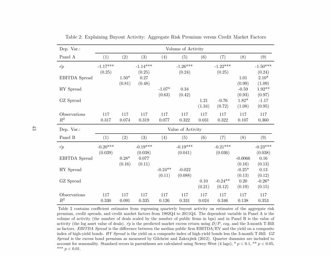
Table 2: Explaining Buyout Activity: Aggregate Risk Premium versus Credit Market Factors
Dep. Var.: Volume of Activity
Panel A (1) (2) (3) (4) (5) (6) (7) (8) (9)
rp -1.17*** -1.14*** -1.26*** -1.22*** -1.50***(0.25) (0.25) (0.24) (0.25) (0.24)
EBITDA Spread 1.50* 0.27 1.01 2.10*(0.81) (0.48) (0.99) (1.09)
HY Spread -1.07* 0.34 -0.59 1.92**(0.63) (0.42) (0.93) (0.97)
GZ Spread 1.21 -0.76 1.82* -1.17(1.34) (0.72) (1.08) (0.95)
Observations 117 117 117 117 117 117 117 117 117R2 0.317 0.074 0.319 0.077 0.322 0.031 0.322 0.107 0.360
Dep. Var.: Value of Activity
Panel B (1) (2) (3) (4) (5) (6) (7) (8) (9)
rp -0.20*** -0.19*** -0.19*** -0.21*** -0.23***(0.039) (0.038) (0.041) (0.036) (0.038)
EBITDA Spread 0.28* 0.077 -0.0066 0.16(0.16) (0.11) (0.16) (0.13)
HY Spread -0.24** -0.022 -0.25* 0.13(0.11) (0.088) (0.13) (0.12)
GZ Spread 0.10 -0.24** 0.20 -0.26*(0.21) (0.12) (0.19) (0.15)
Observations 117 117 117 117 117 117 117 117 117R2 0.330 0.091 0.335 0.126 0.331 0.024 0.346 0.138 0.353
Table 2 contains coefficient estimates from regressing quarterly buyout activity on estimates of the aggregate riskpremium, credit spreads, and credit market factors from 1982Q4 to 2011Q4. The dependent variable in Panel A is thevolume of activity (the number of deals scaled by the number of public firms in bps) and in Panel B is the value ofactivity (the log asset value of deals). rp is the predicted market excess return using D/P , cay, and the 3-month T-Billas factors. EBITDA Spread is the difference between the median public firm EBITDA/EV and the yield on a compositeindex of high-yield bonds. HY Spread is the yield on a composite index of high-yield bonds less the 3-month T-Bill. GZSpread is the excess bond premium as measured by Gilchrist and Zakrajsek (2012). Quarter dummies are included toaccount for seasonality. Standard errors in parentheses are calculated using Newey-West (4 lags); * p < 0.1, ** p < 0.05,*** p < 0.01.
43
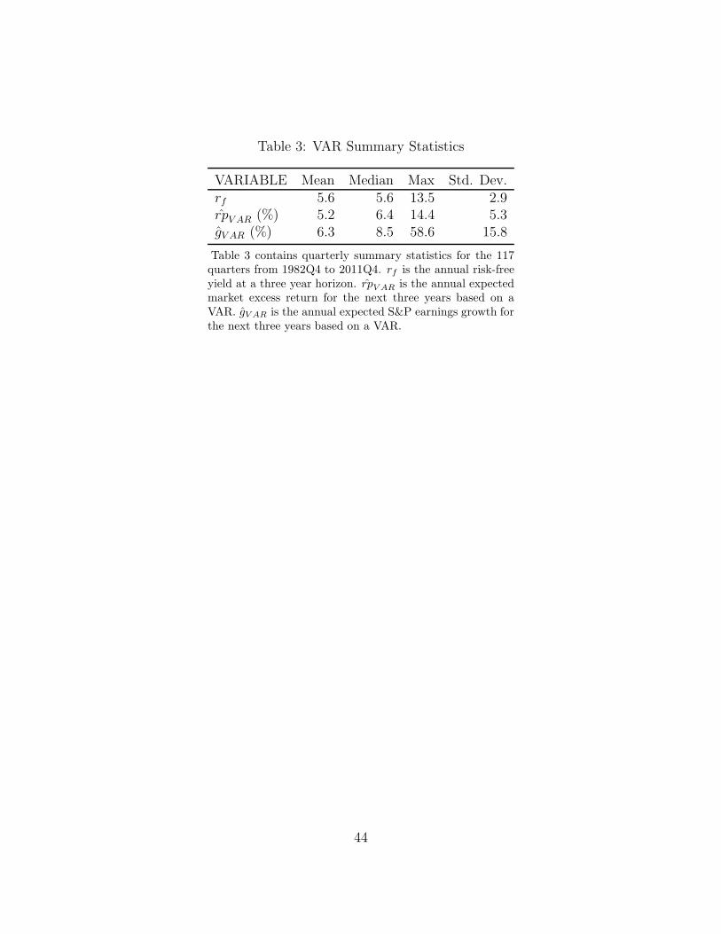
Table 3: VAR Summary Statistics
VARIABLE Mean Median Max Std. Dev.rf 5.6 5.6 13.5 2.9rpV AR (%) 5.2 6.4 14.4 5.3gV AR (%) 6.3 8.5 58.6 15.8
Table 3 contains quarterly summary statistics for the 117quarters from 1982Q4 to 2011Q4. rf is the annual risk-freeyield at a three year horizon. rpV AR is the annual expectedmarket excess return for the next three years based on aVAR. gV AR is the annual expected S&P earnings growth forthe next three years based on a VAR.
44

Table 4: OLS: Buyout Activity on Discount Rates and Growth
Volume Value
(1) (2) (3) (4) (5) (6) (7) (8)
rp -0.88*** -1.20*** -1.41*** -1.09*** -0.18*** -0.22*** -0.26*** -0.14**(0.33) (0.33) (0.32) (0.37) (0.053) (0.051) (0.054) (0.060)
g 0.23*** 0.30*** 0.25** 0.031*** 0.047*** 0.035***(0.072) (0.095) (0.10) (0.010) (0.012) (0.010)
rf 0.82 2.65** 0.17** 0.66***(0.57) (1.14) (0.068) (0.12)
EBITDA Spread 1.46 0.041(1.19) (0.15)
HY Spread -0.83 -0.51***(1.26) (0.17)
GZ Spread 5.43*** 1.26***(1.97) (0.24)
Observations 117 117 117 117 117 117 117 117R2 0.176 0.247 0.277 0.348 0.247 0.296 0.345 0.457
Table 4 contains coefficient estimates from regressing quarterly buyout activity on the components of a Campbell-Shiller decom-position at a three-year horizon from 1982Q4 to 2011Q4. The dependent variable in Columns (1)-(4) is the volume of activity(the number of deals scaled by the number of public firms in bps) and in Columns (5)-(8) is the value of activity (the log assetvalue of deals). rp is the annual expected market excess return for the next three years based on a VAR. g is the annual expectedS&P earnings growth for the next three years based on a VAR. rf is the annual risk-free yield at a three year horizon. EBITDASpread is the difference between the median public firm EBITDA/EV and the yield on a composite index of high-yield bonds.HY Spread is the yield on a composite index of high-yield bonds less the 3-month T-Bill. GZ Spread is the excess bond premiumas measured by Gilchrist and Zakrajsek (2012). Quarter dummies are included to account for seasonality. Standard errors inparentheses are calculated using Newey-West (4 lags); * p < 0.1, ** p < 0.05, *** p < 0.01.
45

Table 5: Buyout Activity on Alternative Measures
VAR: Dividends rpOLS, gIBES rpOLS, gEBIT rpActual, gEBIT
(1) (2) (3) (4) (5) (6) (7) (8)
rp -0.96*** -0.72* -1.42*** -1.29*** -1.34*** -1.30*** -0.52*** -0.50***(0.31) (0.40) (0.22) (0.28) (0.22) (0.30) (0.15) (0.15)
g 0.34 0.29 0.15** 0.16** 0.22* 0.30** 0.32** 0.38**(0.48) (0.46) (0.074) (0.076) (0.12) (0.15) (0.15) (0.16)
rf 0.24 2.31** 1.04* 1.93** 0.88* 1.56* -0.082 2.40***(0.49) (1.03) (0.53) (0.86) (0.52) (0.84) (0.51) (0.78)
EBITDA Spread 5.72*** 2.88* 3.13* 7.36***(1.92) (1.52) (1.75) (1.66)
HY Spread 2.32* 2.00* 1.67 2.50**(1.25) (1.10) (1.02) (1.14)
GZ Spread -0.52 0.40 0.81 -0.38(1.28) (0.86) (0.89) (1.08)
Observations 117 117 116 116 113 113 113 113R2 0.200 0.302 0.374 0.413 0.388 0.435 0.248 0.409
Table 5 contains coefficient estimates from regressing quarterly buyout activity on alternative estimates of growth and therisk premium from 1982Q4 to 2011Q4. The dependent variable is the volume of activity scaled by the number of publicfirms (in basis points). (1)-(2), rp is the expected market excess return based on a VAR using dividend growth ratherthan earnings growth. g is expected S&P dividend growth based on a VAR. (3)-(4), rp is the predicted market excessreturn using D/P , cay, and the 3-month T-Bill as factors. g is the mean IBES estimate of S&P dividend growth for thenext two years. (5)-(6), rp is the predicted market excess return using D/P , cay, and the 3-month T-Bill as factors. gis the actual aggregate EBIT growth for the next year for firms in Compustat. (7)-(8), rp is the actual annual marketreturn for the next three years. g is the actual aggregate EBIT growth for the next year for firms in Compustat. rf is therisk-free yield at a three year horizon. EBITDA Spread is the difference between the median public firm EBITDA/EVand the yield on a composite index of high-yield bonds. HY Spread is the yield on a a composite index of high-yield bondsless the 3-month T-Bill. GZ Spread is the excess bond premium as measured by Gilchrist and Zakrajsek (2012). Quarterdummies are included to account for seasonality. Standard errors in parentheses are calculated using Newey-West (4 lags);* p < 0.1, ** p < 0.05, *** p < 0.01.
46

Table 6: Summary of Firm-Quarters: Full Sample and LBO Firm-Quarters
All Firm-Quarters LBO Firm-Quarters
VARIABLE N Mean Median Std. Dev. N Mean Median Std. Dev.
Deal Dummy 501,176 0.002 0.000 0.046 1,043 1.000 1.000 0.000
Firm Characteristics:
Assets (mm) 501,176 $2,027 $155 $12,728 1,043 $978 $211 $2,960log(Assets) 501,176 5.19 5.04 2.13 1,043 5.48 5.35 1.59EBITDA/Assets 487,597 0.05 0.11 0.22 1,031 0.11 0.13 0.15CapEx/Sales 485,577 0.14 0.04 0.39 1,030 0.07 0.03 0.17R&D/Sales 485,195 0.16 0.00 0.84 1,030 0.03 0.00 0.18Net Debt/Assets 494,072 0.07 0.11 0.36 1,035 0.14 0.18 0.35Turnover 488,367 1.15 0.63 1.89 1,036 1.05 0.59 3.73Dividend Dummy 501,176 0.32 0.00 0.46 1,043 0.31 0.00 0.46Book/Market 484,578 0.74 0.55 0.71 998 0.94 0.74 0.79Risk Proxies:
σ(R) 431,467 15.83 13.44 10.69 963 14.26 12.25 8.22β 387,071 0.88 0.78 0.65 899 0.78 0.69 0.59σ(ε) 430,077 11.65 9.24 9.61 959 9.44 8.01 6.72σ(EBITDA/Assets) 488,410 0.12 0.08 0.14 992 0.08 0.05 0.08
Table 6 contains summary statistics for the sample of firm-quarters from 1982Q4 to 2011Q4. Assets are book assets in2010 dollars. Accounting ratios trimmed at the 99% level. Dividend Dummy is equal to one if the firm pays a dividend.σ(R) is the standard deviation of the prior two-years monthly returns. σ(EBITDA/Assets) is the standard deviationof the EBITDA-to-assets ratio over the observable life of a firm. β is the unlevered market beta of the firm based onlagged two-years of monthly returns. σ(ε) is the standard deviation of the unlevered residuals from the market regression.Unlevered betas and residuals are trimmed at the top and bottom 5% to remove extreme outliers. Deal Dummy is equal toone if a firm announces a deal in the upcoming quarter.
47

Table 7: Deal Likelihood and Discount Rates
(1) (2) (3) (4) (5) (6) (7) (8) (9) (10) (11)
rpOLS -2.39*** -2.29*** -2.15*** -2.27*** -1.59***(0.28) (0.28) (0.29) (0.29) (0.35)
rpV AR -0.61*** -0.57***(0.11) (0.13)
gV AR 0.11*** 0.12***(0.031) (0.032)
rf -4.16*** -2.98***(0.47) (1.01)
EBITDA Spread 2.58** 1.22 -1.11 0.36 -0.088(1.00) (0.97) (1.98) (2.36) (2.26)
HY Spread -2.90*** -1.13 -5.24*** -2.63 -0.90(0.75) (0.71) (1.37) (1.72) (1.93)
GZ Spread 5.97*** 4.47*** 10.4*** 7.83*** 3.65(1.41) (0.97) (1.42) (1.35) (2.41)
Firm FE X X X X X X X X X X X
Observations 501,176 501,176 501,176 501,176 501,176 501,176 501,176 501,176 501,176 501,176 501,176R2 0.064 0.063 0.064 0.063 0.064 0.063 0.064 0.064 0.064 0.064 0.064
Table 7 contains coefficient estimates from regressing quarterly deal indicator (Deal) on the risk premium, credit market factors, and firm fixed effects from 1982Q4to 2011Q4. rpOLS is the predicted market excess return using D/P , cay, and the 3-month T-Bill as factors. rpV AR is the annual expected market excess returnfor the next three years based on a VAR. gV AR is the annual expected S&P earnings growth for the next three years based on a VAR. rf is the annual risk-freeyield at a three year horizon. EBITDA Spread is the difference between the median public firm EBITDA/EV and the yield on a composite index of high-yieldbonds. HY Spread is the yield on a a composite index of high-yield bonds less the 3-month T-Bill. GZ Spread is the excess bond premium as measured by Gilchristand Zakrajsek (2012). Quarter dummies are included to account for seasonality. Standard errors in parentheses are calculated by clustering two-ways (by firm andquarter); * p < 0.1, ** p < 0.05, *** p < 0.01.
48
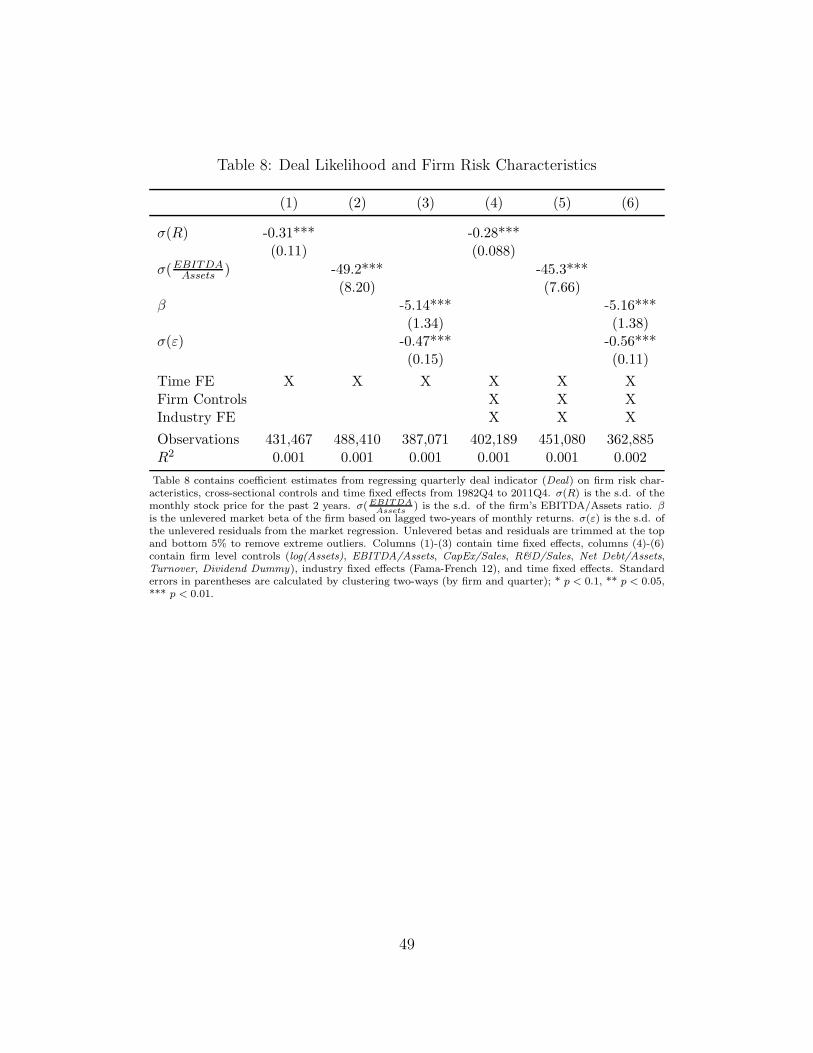
Table 8: Deal Likelihood and Firm Risk Characteristics
(1) (2) (3) (4) (5) (6)
σ(R) -0.31*** -0.28***(0.11) (0.088)
σ(EBITDAAssets ) -49.2*** -45.3***
(8.20) (7.66)β -5.14*** -5.16***
(1.34) (1.38)σ(ε) -0.47*** -0.56***
(0.15) (0.11)
Time FE X X X X X XFirm Controls X X XIndustry FE X X X
Observations 431,467 488,410 387,071 402,189 451,080 362,885R2 0.001 0.001 0.001 0.001 0.001 0.002
Table 8 contains coefficient estimates from regressing quarterly deal indicator (Deal) on firm risk char-acteristics, cross-sectional controls and time fixed effects from 1982Q4 to 2011Q4. σ(R) is the s.d. of themonthly stock price for the past 2 years. σ(EBITDA
Assets) is the s.d. of the firm’s EBITDA/Assets ratio. β
is the unlevered market beta of the firm based on lagged two-years of monthly returns. σ(ε) is the s.d. ofthe unlevered residuals from the market regression. Unlevered betas and residuals are trimmed at the topand bottom 5% to remove extreme outliers. Columns (1)-(3) contain time fixed effects, columns (4)-(6)contain firm level controls (log(Assets), EBITDA/Assets, CapEx/Sales, R&D/Sales, Net Debt/Assets,Turnover, Dividend Dummy), industry fixed effects (Fama-French 12), and time fixed effects. Standarderrors in parentheses are calculated by clustering two-ways (by firm and quarter); * p < 0.1, ** p < 0.05,*** p < 0.01.
49
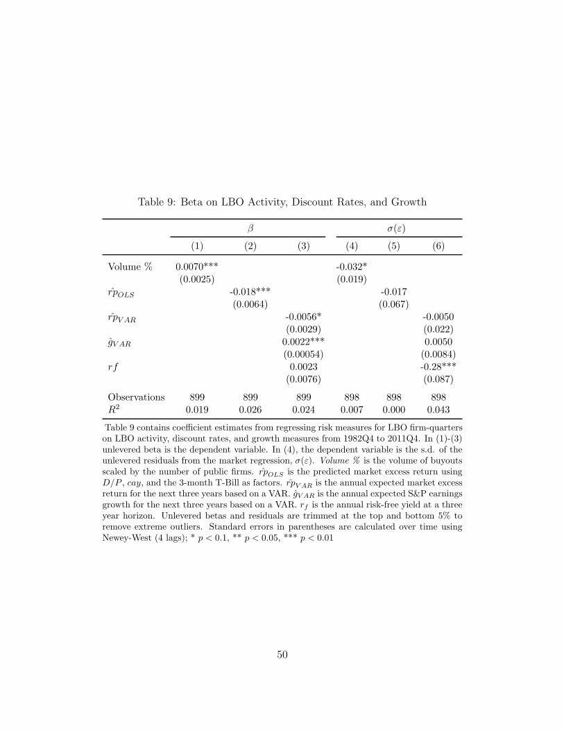
Table 9: Beta on LBO Activity, Discount Rates, and Growth
β σ(ε)
(1) (2) (3) (4) (5) (6)
Volume % 0.0070*** -0.032*(0.0025) (0.019)
rpOLS -0.018*** -0.017(0.0064) (0.067)
rpV AR -0.0056* -0.0050(0.0029) (0.022)
gV AR 0.0022*** 0.0050(0.00054) (0.0084)
rf 0.0023 -0.28***(0.0076) (0.087)
Observations 899 899 899 898 898 898R2 0.019 0.026 0.024 0.007 0.000 0.043
Table 9 contains coefficient estimates from regressing risk measures for LBO firm-quarterson LBO activity, discount rates, and growth measures from 1982Q4 to 2011Q4. In (1)-(3)unlevered beta is the dependent variable. In (4), the dependent variable is the s.d. of theunlevered residuals from the market regression, σ(ε). Volume % is the volume of buyoutsscaled by the number of public firms. rpOLS is the predicted market excess return usingD/P , cay, and the 3-month T-Bill as factors. rpV AR is the annual expected market excessreturn for the next three years based on a VAR. gV AR is the annual expected S&P earningsgrowth for the next three years based on a VAR. rf is the annual risk-free yield at a threeyear horizon. Unlevered betas and residuals are trimmed at the top and bottom 5% toremove extreme outliers. Standard errors in parentheses are calculated over time usingNewey-West (4 lags); * p < 0.1, ** p < 0.05, *** p < 0.01
50

Table 10: Elasticity of Buyout Activity to the Risk Premium – High-LowComparisons
Panel A (1) (2) (3) (4)
Characteristic (X): β GIM EBITDA/Assets Industry HHI
(X)rp -0.026* -0.058** -0.0099 -0.044***(0.014) (0.025) (0.011) (0.015)
Time FE X X X X
Observations 234 174 234 234R2 0.015 0.030 0.002 0.028
Panel B (1) (2) (3) (4)
Characteristic (X): M&A Vol. M&A Val. IPO Vol. IPO Val.
(X)rp 0.060*** 0.015 0.021* 0.024*(0.014) (0.013) (0.013) (0.013)
Time FE X X X X
Observations 234 234 234 234R2 0.085 0.006 0.012 0.015
Table 10 contains coefficient estimates estimating the differential sensitivity of high andlow quartile portfolios to changes in the risk premium. Specifically, we regress deal ac-tivity scaled by its average on a dummy variable indicating the high quartile for a givencharacteristic, and interaction of the dummy with the risk premium and time fixed effectsfrom 1982Q4 to 2011Q4. rp is the predicted market excess return using D/P , cay, and the3-month T-Bill as factors. In Panel A the portfolios and top quartile dummies are basedon the following: β, the unlevered market beta of the firm; GIM , the Governance Indexof the firm (Gompers et al., 2003); EBITDA/Assets, EBITDA/Assets, HHI the HHI ofsales for public firms in the three-digit SIC code. In Panel B the portfolios and top quartiledummies are based on M&A and IPO activity in a Fama-French 48 industry. Activity isbased on a three-year moving average. Volumes are scaled by the number of public firms inthe industry, values are scaled by the value of public firms in the industry. Standard errorsin parentheses are calculated by clustering two-ways (by portfolio and quarter); * p < 0.1,** p < 0.05, *** p < 0.01.
51
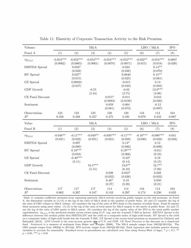
Table 11: Elasticity of Corporate Transaction Activity to the Risk Premium
Volume: M&A LBO / M&A IPO
Panel A (1) (2) (3) (4) (5) (6) (7) (8)
rpOLS -0.054*** -0.052*** -0.054*** -0.054*** -0.052*** -0.032** -0.054*** 0.0087(0.0062) (0.0065) (0.0061) (0.0078) (0.0071) (0.015) (0.018) (0.026)
EBITDA Spread 0.058* 0.033 0.14**(0.033) (0.038) (0.070)
HY Spread 0.027* 0.0040 0.15**(0.015) (0.025) (0.061)
GZ Spread 0.00024 -0.015 0.13(0.047) (0.040) (0.082)
GDP Growth -0.55 -0.82 13.9***(2.44) (2.75) (3.96)
CE Fund Discount 0.015* 0.014 0.010(0.0083) (0.0100) (0.020)
Sentiment 0.059 0.064 -0.12(0.081) (0.073) (0.097)
Observations 123 123 123 120 120 116 113 164R2 0.456 0.488 0.457 0.475 0.491 0.079 0.242 0.007
Value: M&A LBO / M&A IPO
Panel B (1) (2) (3) (4) (5) (6) (7) (8)
rpOLS -0.048** -0.11*** -0.049** -0.056*** -0.11*** -0.10*** -0.080*** 0.041(0.021) (0.023) (0.021) (0.021) (0.028) (0.030) (0.028) (0.033)
EBITDA Spread 0.097 0.14* 0.12(0.080) (0.086) (0.099)
HY Spread 0.19*** 0.19*** -0.011(0.053) (0.066) (0.10)
GZ Spread -0.40*** -0.23* 0.18(0.11) (0.14) (0.15)
GDP Growth 18.4*** 13.6** 16.7**(5.15) (6.10) (7.80)
CE Fund Discount 0.039 0.045* 0.028(0.032) (0.026) (0.032)
Sentiment 0.46* 0.18 0.050(0.27) (0.20) (0.21)
Observations 117 117 117 114 114 116 113 164R2 0.062 0.207 0.187 0.143 0.297 0.174 0.230 0.032
Table 11 contains coefficient estimates from regressing quarterly M&A activity involving public targets on the risk premium. In PanelA, the dependent variable in (1)-(5) is the log of the ratio of M&A deals to the number of public firms. (6) and (7) consider the log ofthe ratio of LBO volume to M&A volume. (9) considers the log of the ratio of IPO deals to the number of public firms. Panel B repeatsthese measures using asset values. (1)-(5) is the log of the ratio of total assets for M&A targets to the assets of public firms. (6) and (7)use the log of the ratio of LBO assets to M&A assets. (9) considers the log of the equity value of the IPO to the total public marketcapitalization. rpOLS is the predicted market excess return using D/P , cay, and the 3-month T-Bill as factors. EBITDA Spread is thedifference between the median public firm EBITDA/EV and the yield on a composite index of high-yield bonds. HY Spread is the yieldon a composite index of high-yield bonds less the 3-month T-Bill. GZ Spread is the excess bond premium as measured by Gilchrist andZakrajsek (2012). GDP Growth is the year-on-year growth rate of U.S. real GDP. CE Fund Discount is the discount on a closed-endfund. Sentiment is a measure of sentiment from Baker and Wurgler (2006). The M&A sample ranges from 1981Q2-2011Q4. TheLBO sample ranges from 1982Q4 to 2011Q4. IPO activity ranges from 1981Q2-2011Q4. Each regression also includes quarter dummyvariables to account for seasonality. Standard errors in parentheses are calculated over time using Newey-West (4 lags); * p < 0.1, **p < 0.05, *** p < 0.01
52

A Model
A.1 Deriving the cost of capital
Pricing on public markets follows the CAPM.
1. Sure payoffs of 1 are discounted at the risk-free rate: NPV(1) = 1/(1 + rf ).
2. Risky market exposure of 1 +Rm = 1+ rf + Rem + εm is discounted using the risk premium:
NPV(1 +Rm) = 1
3. Idiosyncratic risk εi is not priced: NPV(εi) = 0.
Then, pricing is additive; the Law of One Price holds: NPV(aX + bY ) = aNPV(X) + bNPV(Y )for any constants a and b and payoffs X and Y .
To understand the equivalence with the standard Discounted Cash-Flow valuation, consider acash-flow that pays one on average and loads on the aggregate risk factor εm. The payoff at time1 is: P1 = 1 + βCFεm. βCF represents the cash-flow exposure of the claim to aggregate risk. Ourmodel of pricing gives immediately the initial price
P0 =1− βCFRe
m
1 + rf.
Alternatively, one can focus on returns. The return on that claim given the initial price P0 is:
Ra =P1
P0− 1 =
1
P0+
βCF
P0εm − 1 =
1
P0+ βRεm − 1.
βR = βCF/P0 is the return exposure of the claim to aggregate risk. Expected returns are E(Ra) =1P0
− 1. According to the CAPM, we estimate the expected return from its covariance with themarket excess return Re
m:
E(Ra) = rf +Cov (Ra, R
em)
Var (Rem)
Rem = rf + βRRe
m
Using this cost of capital to discount expected cash-flow, following DCF valuation, we obtain
PDCF0 =
1
1 + rf + βRRem
It is immediate to verify that P0 = PDCF0 . Hence valuations follow the classic DCF formula with
risk adjustment.
A.2 Allowing for benchmarking.
We extend the contracting space to allow for the benchmarking of contracts. To do so we allowcontracts to have a component depending on the market structure parameterized by k2. The payout
53

to the private equity investor becomes k0 + k1pH Y + k2(Rem + εm). Following Equation (3), we
represent the payoff as a portfolio:
θ0 = k0 + k1pH(µ − βRem)
θm = k1pHβ + k2
θi = k1pH
This market loading k2 is costless to provide for outside investors because (Rem + εm) is a
zero cost portfolio. It does not affect the IC constraint as the GP receives it independently of itsmanagement decision. The only effect is in the IR constraint through the first-term of the right-hand side of Equation (4), the cost of bearing an inadequate amount of market risk. The optimalchoice of k2 is then clearly to cancel out this term, so that the net exposure θm coincides with θ∗.This corresponds to k2 = 1− k1pH .
Once the illiquidity cost of excess market risk disappears, the condition for the feasibility of adeal becomes
(pH − 1)(µ− βRe
m
)≥
1
2γσ2
i k∗21 p2Hσ2
i .
Benchmarking with pre-contracting. While benchmarking of contracts is useful, it is notalways possible given the timing of private equity contracting. Similarly to Ewens et al. (2013), weassume the contract has to be specified before the target is known. There are two equally likelytargets with market exposure β and β, and otherwise identical.
We look for a pre-specified contract where both outside investors and the GP benefit by par-ticipating. The problem is
min(k0,k1)
k0 + k1pH(µ− βRem)−W0(1 + rf )
s.t. k1 ≥ b/∆p (IC)
k0 + k1pH
(
µ−β + β
2Re
m
)
−W0(1 + rf ) ≥
1
4γσ2
m
[(k1pHβ + k2 − θ∗m)2 + (k1pH β + k2 − θ∗m)2
]+
1
2γσ2
i k21p
2Hσ2
i (IR)
The optimal choice of k2 minimizes the illiquidity cost but they do not reach 0. The condition forsuch an arrangement to be feasible is
(pH − 1)
(
µ−β + β
2Re
m
)
≥1
2γσ2
m(k∗1pH)2
(
β + β
2
)2
+1
2γσ2
i k∗21 p2Hσ2
i
We see that the illiquidity channel is still present through inadequate amounts of aggregate risk,and that this cost increases with the risk premium. The reason for this effect is that while the
54
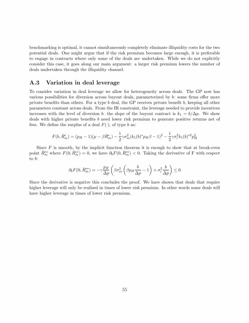
benchmarking is optimal, it cannot simultaneously completely eliminate illiquidity costs for the twopotential deals. One might argue that if the risk premium becomes large enough, it is preferableto engage in contracts where only some of the deals are undertaken. While we do not explicitlyconsider this case, it goes along our main argument: a larger risk premium lowers the number ofdeals undertaken through the illiquidity channel.
A.3 Variation in deal leverage
To consider variation in deal leverage we allow for heterogeneity across deals. The GP now hasvarious possibilities for diversion across buyout deals, parameterized by b: some firms offer moreprivate benefits than others. For a type b deal, the GP receives private benefit b, keeping all otherparameters constant across deals. From the IR constraint, the leverage needed to provide incentivesincreases with the level of diversion b: the slope of the buyout contract is k1 = b/∆p. We showdeals with higher private benefits b need lower risk premium to generate positive returns net offees. We define the surplus of a deal F (·), of type b as:
F (b, Rem) = (pH − 1)(µ − βRe
m)−1
2γσ2
m(k1(b)∗pHβ − 1)2 −
1
2γσ2
i k1(b)∗2p2H
Since F is smooth, by the implicit function theorem it is enough to show that at break-evenpoint Re∗
m where F (0, Re∗m ) = 0, we have ∂bF (0, Re∗
m ) < 0. Taking the derivative of F with respectto b:
∂bF (0, Re∗m ) = −γ
pH∆p
(
βσ2m
(
βpHb
∆p− 1
)
+ σ2i
b
∆p
)
≤ 0
Since the derivative is negative this concludes the proof. We have shown that deals that requirehigher leverage will only be realised in times of lower risk premium. In other words some deals willhave higher leverage in times of lower risk premium.
55

B Supplementary Empirical Appendix
Table 12: Correlation Table
rpOLS EBITDA Sprd. HY Sprd. GZ Sprd. rpV AR gV AR rf
rpOLS 1.00EBITDA Spread -0.36 1.00HY Spread 0.55 -0.85 1.00GZ Spread -0.32 -0.22 0.16 1.00rpV AR 0.85 -0.25 0.52 -0.11 1.00gV AR 0.09 0.27 -0.09 0.09 0.47 1.00rf 0.42 -0.40 0.53 -0.61 0.22 -0.28 1.00
Table 12 contains correlation coefficients between explanatory variables. rpOLS is the predicted marketexcess return using D/P , cay, and the 3-month T-Bill as factors. EBITDA Spread is the differencebetween the median public firm EBITDA/EV and the yield on a composite index of high-yield bonds.HY Spread is the yield on a a composite index of high-yield bonds less the 3-month T-Bill. GZ Spreadis the excess bond premium as measured by Gilchrist and Zakrajsek (2012). rpV AR is the annualexpected market excess return for the next three years based on a VAR. g is the annual expectedS&P earnings growth for the next three years based on a VAR. rf is the risk-free yield at a three-yearhorizon.
56
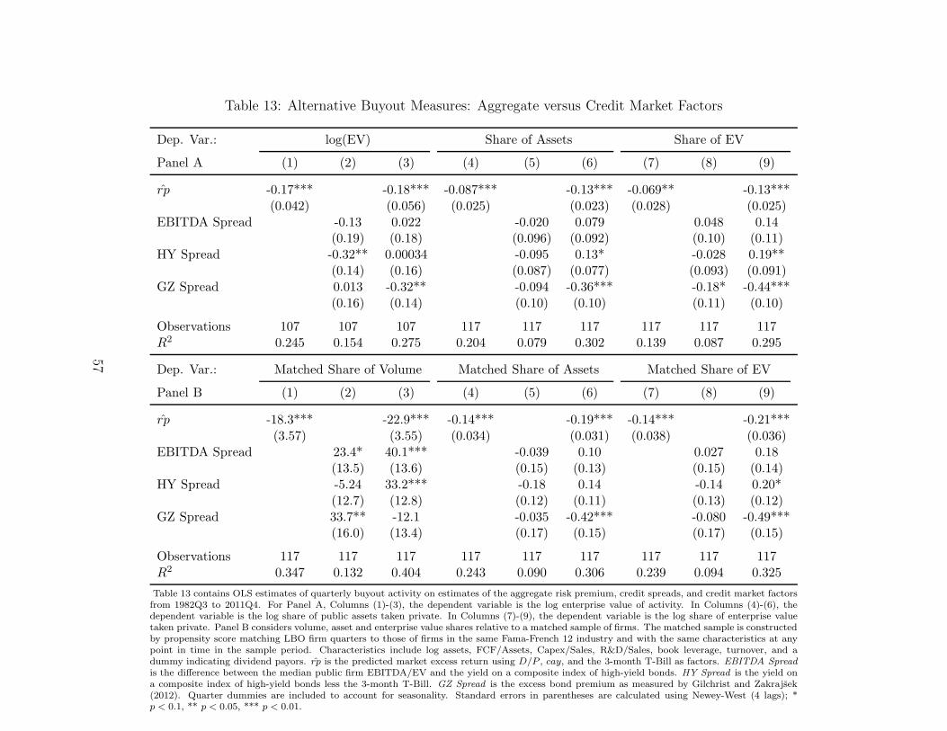
Table 13: Alternative Buyout Measures: Aggregate versus Credit Market Factors
Dep. Var.: log(EV) Share of Assets Share of EV
Panel A (1) (2) (3) (4) (5) (6) (7) (8) (9)
rp -0.17*** -0.18*** -0.087*** -0.13*** -0.069** -0.13***(0.042) (0.056) (0.025) (0.023) (0.028) (0.025)
EBITDA Spread -0.13 0.022 -0.020 0.079 0.048 0.14(0.19) (0.18) (0.096) (0.092) (0.10) (0.11)
HY Spread -0.32** 0.00034 -0.095 0.13* -0.028 0.19**(0.14) (0.16) (0.087) (0.077) (0.093) (0.091)
GZ Spread 0.013 -0.32** -0.094 -0.36*** -0.18* -0.44***(0.16) (0.14) (0.10) (0.10) (0.11) (0.10)
Observations 107 107 107 117 117 117 117 117 117R2 0.245 0.154 0.275 0.204 0.079 0.302 0.139 0.087 0.295
Dep. Var.: Matched Share of Volume Matched Share of Assets Matched Share of EV
Panel B (1) (2) (3) (4) (5) (6) (7) (8) (9)
rp -18.3*** -22.9*** -0.14*** -0.19*** -0.14*** -0.21***(3.57) (3.55) (0.034) (0.031) (0.038) (0.036)
EBITDA Spread 23.4* 40.1*** -0.039 0.10 0.027 0.18(13.5) (13.6) (0.15) (0.13) (0.15) (0.14)
HY Spread -5.24 33.2*** -0.18 0.14 -0.14 0.20*(12.7) (12.8) (0.12) (0.11) (0.13) (0.12)
GZ Spread 33.7** -12.1 -0.035 -0.42*** -0.080 -0.49***(16.0) (13.4) (0.17) (0.15) (0.17) (0.15)
Observations 117 117 117 117 117 117 117 117 117R2 0.347 0.132 0.404 0.243 0.090 0.306 0.239 0.094 0.325
Table 13 contains OLS estimates of quarterly buyout activity on estimates of the aggregate risk premium, credit spreads, and credit market factorsfrom 1982Q3 to 2011Q4. For Panel A, Columns (1)-(3), the dependent variable is the log enterprise value of activity. In Columns (4)-(6), thedependent variable is the log share of public assets taken private. In Columns (7)-(9), the dependent variable is the log share of enterprise valuetaken private. Panel B considers volume, asset and enterprise value shares relative to a matched sample of firms. The matched sample is constructedby propensity score matching LBO firm quarters to those of firms in the same Fama-French 12 industry and with the same characteristics at anypoint in time in the sample period. Characteristics include log assets, FCF/Assets, Capex/Sales, R&D/Sales, book leverage, turnover, and adummy indicating dividend payors. rp is the predicted market excess return using D/P , cay, and the 3-month T-Bill as factors. EBITDA Spreadis the difference between the median public firm EBITDA/EV and the yield on a composite index of high-yield bonds. HY Spread is the yield ona composite index of high-yield bonds less the 3-month T-Bill. GZ Spread is the excess bond premium as measured by Gilchrist and Zakrajsek(2012). Quarter dummies are included to account for seasonality. Standard errors in parentheses are calculated using Newey-West (4 lags); *p < 0.1, ** p < 0.05, *** p < 0.01.
57

Table 14: Private-to-Private Buyout Activity: Aggregate Risk Premium versus Credit Market Factors
Dep. Var.: Private-to-Private Volume
(1) (2) (3) (4) (5) (6) (7) (8) (9)
rp -3.60*** -3.22*** -2.86*** -3.55*** -2.43**(0.89) (0.85) (0.86) (0.96) (1.06)
EBITDA Spread 6.60*** 3.13* -1.20 0.57(2.43) (1.90) (2.79) (2.91)
HY Spread -5.98*** -2.78* -7.26*** -3.20(2.03) (1.64) (2.58) (2.52)
GZ Spread 6.51* 0.77 8.89*** 4.05(3.57) (3.29) (3.16) (4.08)
Observations 117 117 117 117 117 117 117 117 117R2 0.391 0.151 0.420 0.257 0.430 0.053 0.392 0.353 0.444
Table 14 contains coefficient estimates from regressing quarterly private-to-private buyout volume on estimates of theaggregate risk premium, credit spreads, and credit market factors from 1982Q4 to 2011Q4. rp is the predicted marketexcess return using D/P , cay, and the 3-month T-Bill as factors. EBITDA Spread is the difference between the medianpublic firm EBITDA/EV and the yield on a composite index of high-yield bonds. HY Spread is the yield on a compositeindex of high-yield bonds less the 3-month T-Bill. GZ Spread is the excess bond premium as measured by Gilchrist andZakrajsek (2012). Quarter dummies are included to account for seasonality. Standard errors in parentheses are calculatedusing Newey-West (4 lags); * p < 0.1, ** p < 0.05, *** p < 0.01.
58

Table 15: Explaining Buyout Activity: Alternative Risk Premium Measures
Activity: Volume rpRolling rpD/P,cay rpActual
Panel A (1) (2) (3) (4) (5) (6)
rp -0.58** -0.76** -0.94*** -1.45*** -0.46*** -0.53***(0.24) (0.31) (0.27) (0.33) (0.14) (0.14)
EBITDA Spread 1.85* 1.19 3.34**(1.07) (1.07) (1.42)
HY Spread 1.33 1.68* 1.11(0.94) (0.90) (1.02)
GZ Spread -1.17 -2.63** 1.82*(1.40) (1.32) (1.02)
Observations 117 117 117 117 113 113R2 0.164 0.191 0.237 0.280 0.166 0.256
Activity: Value rpRolling rpD/P,cay rpActual
Panel B (1) (2) (3) (4) (5) (6)
rp -0.091*** -0.087* -0.15*** -0.21*** -0.061*** -0.057***(0.034) (0.046) (0.043) (0.057) (0.020) (0.019)
EBITDA Spread 0.091 0.020 0.24(0.14) (0.14) (0.19)
HY Spread -0.030 0.069 -0.073(0.16) (0.14) (0.13)
GZ Spread -0.15 -0.43* 0.19(0.26) (0.24) (0.19)
Observations 117 117 117 117 113 113R2 0.153 0.179 0.232 0.266 0.113 0.197
Table 15 contains coefficient estimates from regressing quarterly buyout activity on estimates ofthe aggregate risk premium, credit spreads, and credit market factors from 1982Q4 to 2011Q4.The dependent variable in Panel A is the volume of activity (the number of deals scaled bythe number of public firms in bps) and in Panel B is the value of activity (the log asset valueof deals). Columns (1)-(2) use a rolling prediction of equity returns where D/P , cay, and the3-month T-Bill are factors. Columns (3)-(4) use an estimate solely based on D/P and cay.Columns (5)-(6) use actual forward excess equity returns. EBITDA Spread is the differencebetween the median public firm EBITDA/EV and the yield on a composite index of high-yieldbonds. HY Spread is the yield on a composite index of high-yield bonds less the 3-month T-Bill.GZ Spread is the excess bond premium as measured by Gilchrist and Zakrajsek (2012). Quarterdummies are included to account for seasonality. Standard errors in parentheses are calculatedusing Newey-West (4 lags); * p < 0.1, ** p < 0.05, *** p < 0.01.
59
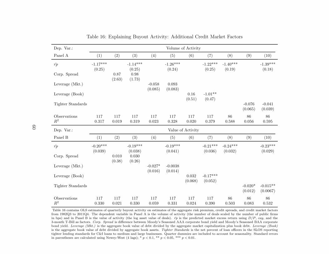
Table 16: Explaining Buyout Activity: Additional Credit Market Factors
Dep. Var.: Volume of Activity
Panel A (1) (2) (3) (4) (5) (6) (7) (8) (9) (10)
rp -1.17*** -1.14*** -1.26*** -1.22*** -1.40*** -1.39***(0.25) (0.25) (0.24) (0.25) (0.19) (0.18)
Corp. Spread 0.87 0.98(2.63) (1.73)
Leverage (Mkt.) -0.058 0.093(0.085) (0.083)
Leverage (Book) 0.16 -1.01**(0.51) (0.47)
Tighter Standards -0.076 -0.041(0.065) (0.039)
Observations 117 117 117 117 117 117 117 86 86 86R2 0.317 0.019 0.319 0.023 0.328 0.020 0.379 0.588 0.056 0.595
Dep. Var.: Value of Activity
Panel B (1) (2) (3) (4) (5) (6) (7) (8) (9) (10)
rp -0.20*** -0.19*** -0.19*** -0.21*** -0.24*** -0.23***(0.039) (0.038) (0.041) (0.036) (0.032) (0.029)
Corp. Spread 0.010 0.030(0.38) (0.26)
Leverage (Mkt.) -0.027* -0.0038(0.016) (0.014)
Leverage (Book) 0.032 -0.17***(0.068) (0.052)
Tighter Standards -0.020* -0.015**(0.012) (0.0067)
Observations 117 117 117 117 117 117 117 86 86 86R2 0.330 0.021 0.330 0.059 0.331 0.024 0.390 0.503 0.083 0.532
Table 16 contains OLS estimates of quarterly buyout activity on estimates of the aggregate risk premium, credit spreads, and credit market factorsfrom 1982Q3 to 2011Q4. The dependent variable in Panel A is the volume of activity (the number of deals scaled by the number of public firmsin bps) and in Panel B is the value of activity (the log asset value of deals). rp is the predicted market excess return using D/P , cay, and the3-month T-Bill as factors. Corp. Spread is difference between Moody’s Seasoned AAA corporate bond yield and Moody’s Seasoned BAA corporatebond yield. Leverage (Mkt.) is the aggregate book value of debt divided by the aggregate market capitalization plus book debt. Leverage (Book)is the aggregate book value of debt divided by aggregate book assets. Tighter Standards is the net percent of loan officers in the SLOS reportingtighter lending standards for C&I loans to medium and large businesses. Quarter dummies are included to account for seasonality. Standard errorsin parentheses are calculated using Newey-West (4 lags); * p < 0.1, ** p < 0.05, *** p < 0.01.
60
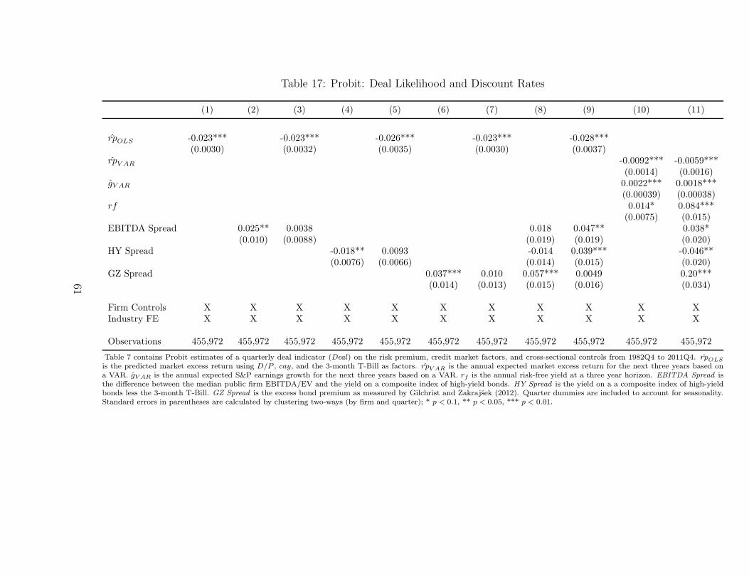
Table 17: Probit: Deal Likelihood and Discount Rates
(1) (2) (3) (4) (5) (6) (7) (8) (9) (10) (11)
rpOLS -0.023*** -0.023*** -0.026*** -0.023*** -0.028***(0.0030) (0.0032) (0.0035) (0.0030) (0.0037)
rpV AR -0.0092*** -0.0059***(0.0014) (0.0016)
gV AR 0.0022*** 0.0018***(0.00039) (0.00038)
rf 0.014* 0.084***(0.0075) (0.015)
EBITDA Spread 0.025** 0.0038 0.018 0.047** 0.038*(0.010) (0.0088) (0.019) (0.019) (0.020)
HY Spread -0.018** 0.0093 -0.014 0.039*** -0.046**(0.0076) (0.0066) (0.014) (0.015) (0.020)
GZ Spread 0.037*** 0.010 0.057*** 0.0049 0.20***(0.014) (0.013) (0.015) (0.016) (0.034)
Firm Controls X X X X X X X X X X XIndustry FE X X X X X X X X X X X
Observations 455,972 455,972 455,972 455,972 455,972 455,972 455,972 455,972 455,972 455,972 455,972
Table 7 contains Probit estimates of a quarterly deal indicator (Deal) on the risk premium, credit market factors, and cross-sectional controls from 1982Q4 to 2011Q4. rpOLS
is the predicted market excess return using D/P , cay, and the 3-month T-Bill as factors. rpV AR is the annual expected market excess return for the next three years based ona VAR. gV AR is the annual expected S&P earnings growth for the next three years based on a VAR. rf is the annual risk-free yield at a three year horizon. EBITDA Spread isthe difference between the median public firm EBITDA/EV and the yield on a composite index of high-yield bonds. HY Spread is the yield on a a composite index of high-yieldbonds less the 3-month T-Bill. GZ Spread is the excess bond premium as measured by Gilchrist and Zakrajsek (2012). Quarter dummies are included to account for seasonality.Standard errors in parentheses are calculated by clustering two-ways (by firm and quarter); * p < 0.1, ** p < 0.05, *** p < 0.01.
61
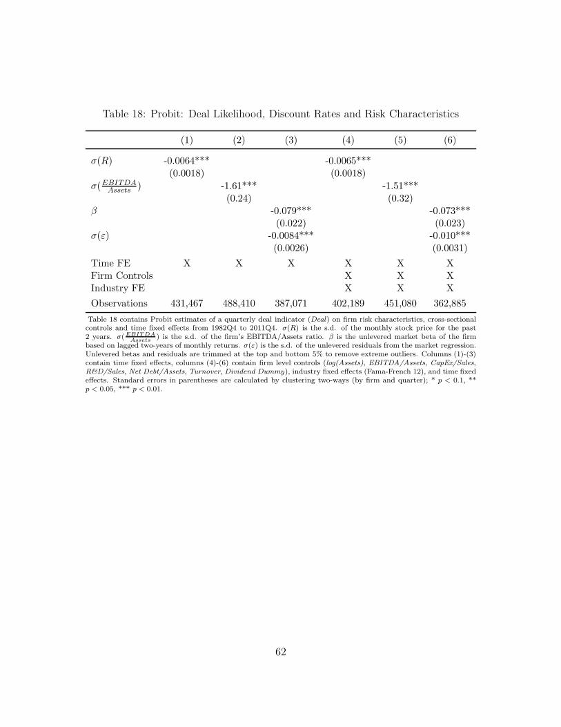
Table 18: Probit: Deal Likelihood, Discount Rates and Risk Characteristics
(1) (2) (3) (4) (5) (6)
σ(R) -0.0064*** -0.0065***(0.0018) (0.0018)
σ(EBITDAAssets ) -1.61*** -1.51***
(0.24) (0.32)β -0.079*** -0.073***
(0.022) (0.023)σ(ε) -0.0084*** -0.010***
(0.0026) (0.0031)
Time FE X X X X X XFirm Controls X X XIndustry FE X X X
Observations 431,467 488,410 387,071 402,189 451,080 362,885
Table 18 contains Probit estimates of a quarterly deal indicator (Deal) on firm risk characteristics, cross-sectionalcontrols and time fixed effects from 1982Q4 to 2011Q4. σ(R) is the s.d. of the monthly stock price for the past2 years. σ(EBITDA
Assets) is the s.d. of the firm’s EBITDA/Assets ratio. β is the unlevered market beta of the firm
based on lagged two-years of monthly returns. σ(ε) is the s.d. of the unlevered residuals from the market regression.Unlevered betas and residuals are trimmed at the top and bottom 5% to remove extreme outliers. Columns (1)-(3)contain time fixed effects, columns (4)-(6) contain firm level controls (log(Assets), EBITDA/Assets, CapEx/Sales,R&D/Sales, Net Debt/Assets, Turnover, Dividend Dummy), industry fixed effects (Fama-French 12), and time fixedeffects. Standard errors in parentheses are calculated by clustering two-ways (by firm and quarter); * p < 0.1, **p < 0.05, *** p < 0.01.
62

Table 19: Elasticity of Deal Activity to the Risk Premium – Full Cross-SectionComparisons
Panel A (1) (2) (3) (4)
Characteristic (X): β GIM EBITDA/Assets Industry HHI
(X)rp -0.016*** -0.013* -0.043*** -0.028(0.0058) (0.0075) (0.0074) (0.044)
Time FE X X X X
Observations 1,170 1,218 1,170 1,170R2 0.003 0.007 0.002 0.000
Panel B (1) (2) (3) (4)
Characteristic (X): M&A Vol. M&A Val. IPO Vol. IPO Val.
(X)rp 1.87* 1.16** -0.025 3.48(1.11) (0.54) (0.95) (5.34)
Time FE X X X X
Observations 4,914 4,914 4,914 4,914R2 0.002 0.001 0.000 0.000
Table 19 contains coefficient estimates estimating the differential sensitivity of portfoliosformed based on characteristics to changes in the risk premium. Specifically, we regressdeal activity scaled by its average on the average value of the characteristic in a portfolioand an interaction of this value with the risk premium, and time fixed effects from 1982Q4to 2011Q4. rp is the predicted market excess return using D/P , cay, and the 3-monthT-Bill as factors. In Panel A the portfolios are based on the following: β, the deciles ofunlevered market beta of the firm; GIM , the Governance Index of the firm (Gompers et al.,2003); EBITDA/Assets, the deciles of EBITDA/Assets, HHI the deciles of HHI of salesfor public firms in the three-digit SIC code. In Panel B the portfolios are based on M&Aand IPO activity in a Fama-French 48 industry. Activity is based on a three-year movingaverage. Volumes are scaled by the number of public firms in the industry, values are scaledby the value of public firms in the industry. Standard errors in parentheses are calculatedby clustering two-ways (by portfolio and quarter); * p < 0.1, ** p < 0.05, *** p < 0.01.
63
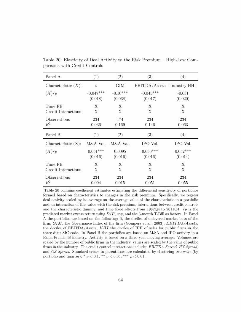
Table 20: Elasticity of Deal Activity to the Risk Premium – High-Low Com-parisons with Credit Controls
Panel A (1) (2) (3) (4)
Characteristic (X): β GIM EBITDA/Assets Industry HHI
(X)rp -0.047*** -0.10*** -0.045*** -0.031(0.018) (0.038) (0.017) (0.020)
Time FE X X X XCredit Interactions X X X X
Observations 234 174 234 234R2 0.036 0.169 0.146 0.063
Panel B (1) (2) (3) (4)
Characteristic (X): M&A Vol. M&A Val. IPO Vol. IPO Val.
(X)rp 0.051*** 0.0095 0.056*** 0.052***(0.016) (0.016) (0.016) (0.014)
Time FE X X X XCredit Interactions X X X X
Observations 234 234 234 234R2 0.094 0.015 0.051 0.055
Table 20 contains coefficient estimates estimating the differential sensitivity of portfoliosformed based on characteristics to changes in the risk premium. Specifically, we regressdeal activity scaled by its average on the average value of the characteristic in a portfolioand an interaction of this value with the risk premium, interactions between credit controlsand the characteristic dummy, and time fixed effects from 1982Q4 to 2011Q4. rp is thepredicted market excess return using D/P , cay, and the 3-month T-Bill as factors. In PanelA the portfolios are based on the following: β, the deciles of unlevered market beta of thefirm; GIM , the Governance Index of the firm (Gompers et al., 2003); EBITDA/Assets,the deciles of EBITDA/Assets, HHI the deciles of HHI of sales for public firms in thethree-digit SIC code. In Panel B the portfolios are based on M&A and IPO activity in aFama-French 48 industry. Activity is based on a three-year moving average. Volumes arescaled by the number of public firms in the industry, values are scaled by the value of publicfirms in the industry. The credit control interactions include: EBITDA Spread, HY Spread,and GZ Spread. Standard errors in parentheses are calculated by clustering two-ways (byportfolio and quarter); * p < 0.1, ** p < 0.05, *** p < 0.01.
64
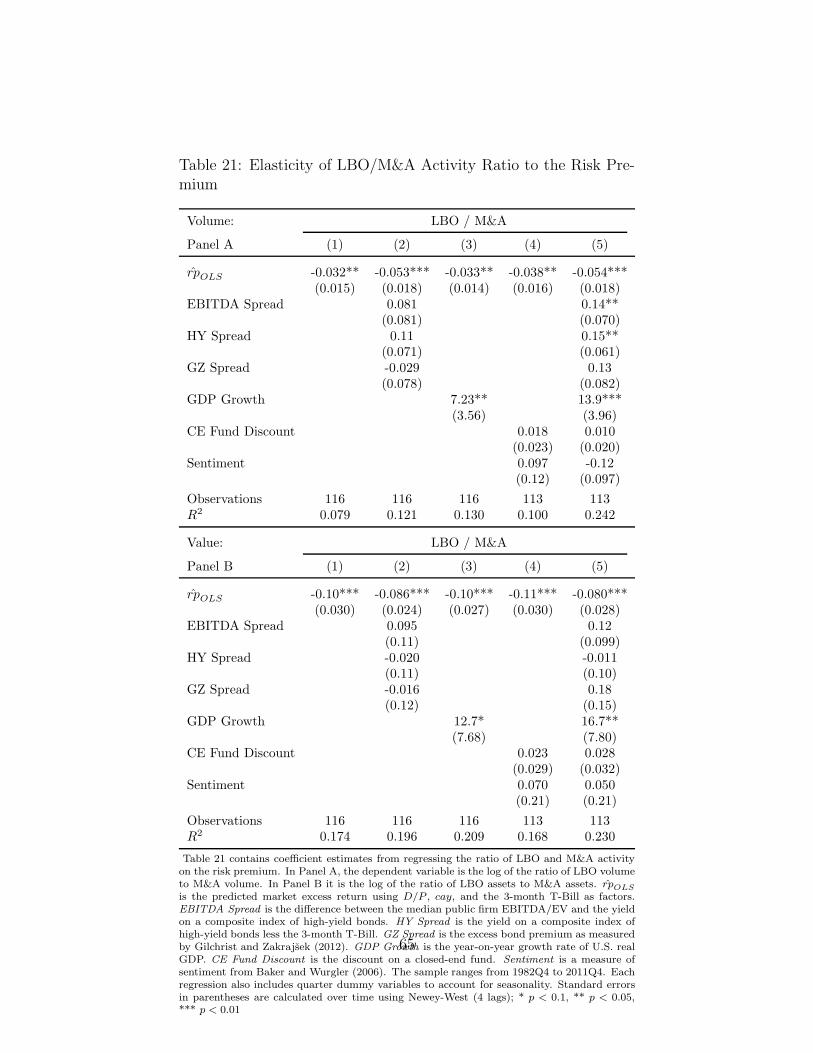
Table 21: Elasticity of LBO/M&A Activity Ratio to the Risk Pre-mium
Volume: LBO / M&A
Panel A (1) (2) (3) (4) (5)
rpOLS -0.032** -0.053*** -0.033** -0.038** -0.054***(0.015) (0.018) (0.014) (0.016) (0.018)
EBITDA Spread 0.081 0.14**(0.081) (0.070)
HY Spread 0.11 0.15**(0.071) (0.061)
GZ Spread -0.029 0.13(0.078) (0.082)
GDP Growth 7.23** 13.9***(3.56) (3.96)
CE Fund Discount 0.018 0.010(0.023) (0.020)
Sentiment 0.097 -0.12(0.12) (0.097)
Observations 116 116 116 113 113R2 0.079 0.121 0.130 0.100 0.242
Value: LBO / M&A
Panel B (1) (2) (3) (4) (5)
rpOLS -0.10*** -0.086*** -0.10*** -0.11*** -0.080***(0.030) (0.024) (0.027) (0.030) (0.028)
EBITDA Spread 0.095 0.12(0.11) (0.099)
HY Spread -0.020 -0.011(0.11) (0.10)
GZ Spread -0.016 0.18(0.12) (0.15)
GDP Growth 12.7* 16.7**(7.68) (7.80)
CE Fund Discount 0.023 0.028(0.029) (0.032)
Sentiment 0.070 0.050(0.21) (0.21)
Observations 116 116 116 113 113R2 0.174 0.196 0.209 0.168 0.230
Table 21 contains coefficient estimates from regressing the ratio of LBO and M&A activityon the risk premium. In Panel A, the dependent variable is the log of the ratio of LBO volumeto M&A volume. In Panel B it is the log of the ratio of LBO assets to M&A assets. rpOLS
is the predicted market excess return using D/P , cay, and the 3-month T-Bill as factors.EBITDA Spread is the difference between the median public firm EBITDA/EV and the yieldon a composite index of high-yield bonds. HY Spread is the yield on a composite index ofhigh-yield bonds less the 3-month T-Bill. GZ Spread is the excess bond premium as measuredby Gilchrist and Zakrajsek (2012). GDP Growth is the year-on-year growth rate of U.S. realGDP. CE Fund Discount is the discount on a closed-end fund. Sentiment is a measure ofsentiment from Baker and Wurgler (2006). The sample ranges from 1982Q4 to 2011Q4. Eachregression also includes quarter dummy variables to account for seasonality. Standard errorsin parentheses are calculated over time using Newey-West (4 lags); * p < 0.1, ** p < 0.05,*** p < 0.01
65