mean and analytical methods to characterize the … · 1laboratoire eole, département...
TRANSCRIPT

1
Mean and analytical methods to characterize the efficiency of floods
to move sediment in a small semi-arid basin
Abdesselam Megnounif1, Sylvain Ouillon2
1Laboratoire EOLE, Département d'hydraulique, Faculté de Technologie, Université Aboubekr Belkaid, Tlemcen, Algeria 2LEGOS, Univ. of Toulouse, IRD, CNRS, CNES, Toulouse, France 5
Correspondence to: Sylvain Ouillon ([email protected])
Abstract. Over a long multi-year period, flood events can be classified according to their effectiveness in moving sediments.
Efficiency depends both on the magnitude and frequency with which events occur. The effective (or dominant) discharge is
the water discharge which corresponds to the maximum sediment supply. If its calculation is well documented in temperate or
humid climate and large basins, it is much more difficult in small and semi-arid basins which encompass short floods with 10
high sediment supplies. On the example of 31-years of measurements in the Wadi Sebdou (North-West Algeria), this paper
compares the two main approaches to calculate the effective discharge (the mean approach based on histograms of sediment
supply by discharge classes and an analytical calculation based on a hydrological probability distribution and on a sediment
rating curve) to a very simple proxy: the half-load discharge, i.e. the flow rate corresponding to 50% of the cumulative sediment
yield. Three types of discharge subdivisions were tested. In the mean approach, two subdivisions provided effective discharges 15
close to the half-load discharge. Analytical solutions based on Log-normal and Log-Gumbel probability distributions were
assessed but they highly underestimated the effective discharge, whatever the subdivision used to adjust the flow frequency
distribution. Furthermore, annual series of maximum discharge and half-load discharge enabled to infer the return period of
hydrological years with discharges higher than the effective discharge (around 2 years) and to show that more than half of the
yearly sediment supply is carried by flows higher than the effective discharge only every 7 hydrological years. This study was 20
the first to adapt the statistical approach in a semi-arid basin and to show the potentiality and limits of each method in a such
climate.
Keywords: sediment transport, effective discharge, return period, semi-arid, Wadi, Algeria
1 Introduction
Over a long multi-year period, flood events can be classified according to their effectiveness in moving sediments. Efficiency 25
depends both on the magnitude and frequency with which events occur. According to Wolman & Miller (1960), the efficiency
can be examined through the ‘sediment transport effectiveness curve’ h(Q) obtained by the product of the two curves f(Q).g(Q),
where f(Q) is the frequency distribution of water discharge, and g(Q) the rating curve estimating the suspended sediment flux
Qs as a function of the water discharge (Fig. 1). Since f(Q) is a bell-shaped probability density function, often adjusted by a
log-normal probability distribution, and g(Q) a function limited in the interval [0; Qmax[ then the function h(Q) goes from 0 30

2
at very low flow rates to almost 0 at the highest flow rates through a maximum. The flow at which the function h reaches its
maximum is the effective discharge, QD, in the sense of Wolman & Miller (1960). The curve h(Q) characterizes the relative
geomorphic work (i.e. the amount of sediment transported) that is carried out in a basin by each flow. The effective discharge
is often referred to as the dominant discharge, which has the greatest role in the formation and maintenance of river
morphology, and whose knowledge is essential for stream restoration projects (Watson et al., 1999). As illustrated in Fig. 1, a 5
large portion of sediment is conceptually transported by weak to moderate floods. Wolman & Miller (1960) confirmed this
concept by comparing the frequency of flows generating suspended sediment transport on watersheds of different sizes in
humid and semi-arid regions and showed that very large devastating floods which produce large amounts of sediments have,
due to their scarcity, a tiny contribution over a long period in front of moderate floods with higher recurrence.
10
Figure 1: Effective discharge curves.
To determine the effective discharge, the mean method is based on the discharge histogram and replaced the sediment-transport
effectiveness function, h(Q), with a sediment supply histogram. The sediment supply histogram results from (Q, C)
measurements or to a discharge histogram – where each class is represented by its mean, which gives its name to the method
– and to a sediment rating curve. The classical method proposed by Benson and Thomas (1966) makes use of a subdivision of 15
discharges into classes of equal amplitude and defined the modal class as the efficient-flow class or dominant class (Dunne
and Leopold, 1978). When series of measurements spans several years, theoretical frequencies are deduced from the frequency
distribution of measured discharges (Andrews, 1980). This approach made it possible to identify the dominant class on many
sites, usually from daily liquid and solid flow series in temperate environments (Ashmore and Day, 1988; Biedenharn et al.,
2001). 20
Alternatively, Nash (1994) proposed an analytical approach to estimate the effective discharge. He argued that for most rivers,
Q
g(Q) f(Q) h(Q)=f(Q).g(Q)
g(Q
) :
Sed
imen
t tr
ansp
ort
rat
e
f(Q
) :
Flo
w f
req
uen
cy
h(Q
) :
Pro
du
ct o
f fr
equ
ency
an
d t
ran
spo
rt r
ate

3
the log-normal distribution adequately represents the flow frequency, and that sediment flow is commonly estimated from a
power model, g(Q)= aQb+1, where a and b are empirical parameters of simple regression established between the Ck and Qk
class representatives (Andrews, 1980; Biedenharn et al., 2001; McKee et al., 2002; Crowder and Knapp, 2005; Bunte et al.,
2014). The probability distribution of discharges and the rating curve of sediment supply provide a mathematical equation of
the sediment transport efficiency curve, h(Q) (Nash, 2004; Vogel et al., 2003). The curve h has a unique maximum reached at 5
the effective rate QD (fig.1), whose analytical expression is solution of the derived function, h’(Q)=0. For more precision and
in order to deal with different flow regimes, the analytical solution of the dominant discharge has been established for
probability distributions other than the log-normal distribution, such as the normal, exponential or log-Pearson III distributions
(Goodwin 2004; West and Niezgoda 2006; Quader et al., 2008; Higgins et al. 2015).
Other methods are still proposed in the literature to estimate the effective discharge. Ferro and Porto (2012), for example, 10
associated it to the flow rate corresponding to 50% of the cumulative sediment yield, thus taking up the concept of "half-load
discharge" introduced by Vogel et al. (2003). Since flows below this threshold carry 50% of the total sediment production and
higher flow rates as much, this flow can also be called a "median water discharge in the sense of sediment yield" (QY50). Other
parameters are calculated in the literature and considered as proxies of the effective discharge, such as the bankfull discharge
(Qb, the discharge which fills the channel to the level of the floodplain, see e.g. Andrews, 1980) or the 1.5 years flow events 15
(Q1.5) (e.g. Crowder and Knapp, 2005; Ferro and Porto, 2012).
These approaches to analyze sediment yield are less well adapted to semi-arid environments that experience the alternation of
very long periods of drought or low flows and sporadic floods. Furthermore, Colombani et al. (1984) and Castillo et al. (2003)
emphasized practical difficulties to control flows and associated matters in small catchments (10 to 104 km2) which are subject
to flash floods that carry significant sediment loads (Reid and Laronne, 1995; Alexandrov et al., 2003; Scott, 2006; Gray et 20
al., 2015) and where accurate sediment records are frequently lacking (Milliman and Syvistki 1992; Biedenharn et al., 2001;
Gray et al. 2015). Probst and Amiotte-Suchet (1992) and Walling (2008) reported that the lack of such series is obvious on the
southern Mediterranean side. Due to the paucity of accurate time series, Crowder and Knapp (2005) highlighted that the
approach developed for identifying the effective discharge has not been verified in watersheds smaller than 518 km2.
In the context of current knowledge and methods, this article proposes to adapt and compare these methods to the hydrology 25
of a small semi-arid basin on an example in Northern Algeria . The application is carried out from 31 years of hydro-
sedimentary measurements on the Wadi Sebdou (1973-2004), on which floods last on average 7.78% of the time. The questions
dealt with in this paper are the following:
1. How can we precondition data series in semi-arid environments?
2. What is the best subdivision of discharge classes adapted to the mean method based on sediment yield histograms? 30
Three types of subdivision are compared.
3. What are the analytical solutions following the Nash's (1994) method which fit statistical probability distributions to
flow histograms to derive the dominant discharge? Theoretical solutions are established for two standard probability
distributions (log-normal, log-Gumbel);

4
4. What are the different sources of errors in each approach?
5. Which lessons can we derive comparing their results and the half-load discharge?
6. Which return periods regarding sediment supply over a long-term period can be derived from the annual series of
hydrological parameters such as the annual maximum discharge and the half-load discharge?
2 Study area and hydrometric measurements 5
The Maghreb is a mountainous region with young relief, characterized by many small watersheds. In these steep marl
landscapes, rainfall erosivity is particularly high (Heusch, 1982; Probst and Amiotte-Suchet, 1992). Located in the north-west
of Algeria, the Wadi Sebdou (or upper Tafna River) runs along 29-km (Fig. 2). The upper reaches emerge through
predominantly carbonate Jurassic terrains at altitudes up to 1400 m. Then the wadi crosses the plain of Sebdou composed of
Plio-quaternary alluviums, and a valley (the gap of Tafna) made up of carbonate rocks (marl-limestone, limestone and Jurassic 10
dolomites) (Benest, 1972; Benest et al., 1992). The Wadi Sebdou flows into the Beni-Bahdel reservoir, with a storage capacity
of 63 million m3, impounded in 1946. The Wadi Sebdou drainage basin area is 256 km2. Steep slopes exceeding 25% represent
about 49% of the total basin surface. The climate is semi-arid. The wet season runs from October to May. The dry season runs
from June to September with low rainfall and high evapotranspiration.
15
Figure 2: Location of the Wadi Sebdou in the Tafna watershed.
Previous studies on sediment dynamics in this basin proposed syntheses on the hydro-sedimentological dynamics and budgets,
or on sediment processes at the origin of hysteresis phenomena during floods, based on the detailed analysis of short-term time

5
variations of water and sediment discharges (Megnounif et al., 2013). Additional and detailed information on morphometric,
geological and land use characteristics of the basin were reported in Bouanani (2004), Megnounif et al. (2013), and Megnounif
and Ghenim (2016).
Discharge and concentration data were measured at the Beni Bahdel station by the National Agency of Hydraulic Resources
(locally called ANRH, www.anrh.dz), in charge of gauging stations and measurements in Algeria. These data cover a 31-year 5
period from September 1973 to August 2004. When water level is low and stable, the operator takes water samples every other
day. During flood periods, sampling is intensified, up to every half hour. During low flow period, water samples are taken
every two weeks. At each sampling, the operator reads the water level on a limnimetric scale or on a limnigraph which is then
converted into a water discharge according to a stage-discharge relationship established for the station. The suspended
sediment concentration is determined from a water sample taken from the streambank, after filtration (see Megnounif et al., 10
2013).
3 Methodology
3.1 Elementary contributions and budgets
The product of discharge, Q in m3 s-1, and suspended sediment concentration, C in g L-1 (or kg m3), make it possible to evaluate
the instantaneous sediment discharge, QS = Q.C in kg s-1. Between two water samples, the liquid flow, Q, and the sediment 15
discharge QS, are assumed to vary linearly. At each flow Qi measured at time ti, is associated a triplet (Δti, ΔRi, ΔYi):
∆ti =1
2(ti+1 − ti) +
1
2(ti − ti−1) =
1
2(ti+1 − ti−1), (1)
∆Ri =1
4[(Qi+1 + Qi)(ti+1 − ti) + (Qi + Qi−1)(ti − ti−1)]10−6, (2)
∆Yi =1
4[(Qi+1Ci+1 + QiCi)(ti+1 − ti) + (QiCi + Qi−1Ci−1)(ti − ti−1)]10−6, (3)
where Δti, ΔRi and ΔYi correspond to time duration (in s), elementary input in water (unit: 106 m3) and elementary sediment 20
yield (unit: 103 tonnes) assigned to the discharge Qi, respectively.
Over a duration T, the water supply RT and sediment yield YT are estimated by summing the elementary contributions:
RT = ∑ ∆Riti∈T YT = ∑ ∆Yiti∈T , (4)
Various quantiles are given using cumulative frequencies and elementary contributions assigned to ordered discharges. The
quantiles QTα, QRα and QYα stand for water discharges that delimit α% of annual time, α% of the total water supply and α% of 25
the sediment yield, respectively. For example, QY50 is the median water discharge in terms of suspended sediment production,
i.e. such that 50% of the sediment yield is carried by discharges lower than QY50.

6
3.2 Effective discharge calculation using a discharge histogram
3.2.1 Basis of the mean method
To analyze flow frequencies and associated sediment yields, the x-axis (discharge) is subdivided into class intervals (or bins)
Ik = [ak, ak+1[ where k = 0, … , N ; a0 ≤ Qmin < a1 and aN ≤ Qmax < aN+1 . The duration, water and sediment yields
attributed to the class Ik are obtained by summing time intervals (eq. 1), water contributions (eq. 2) and sediment yields (eq. 5
3) assigned to discharges Qi within this class, following:
∆Tk = ∑ ∆TiQi∈Ik ; ∆Rk = ∑ ∆RiQi∈Ik
and ∆Yk = ∑ ∆YiQi∈Ik . (5)
Each discharge class, Ik, is represented by a pair (Qk, Ck) where Qk is the midpoint and Ck is the mean sediment concentration
calculated by the equation:
Ck = ∆Yk
∆Rk (6) 10
Discharge classes are examined according to their effectiveness to produce sediments. The discharge class that carries out the
highest sediment yields over an extended period is the dominant class. For simplicity, its midpoint, QD, is the effective
discharge (or dominant discharge). In this article, three ways to subdivide the discharge-axis are presented, applied and
compared.
3.2.2 Class interval assignment 15
Regarding the choice of discharge classes, the procedure is empirical and varies according to the authors (Pickup and Warner,
1976; Andrews, 1980; Lenzi et al., 2006). Biedenharn et al. (2001) recommended starting by the use of 25 classes of equal
lengths. If no measurement is assigned to a class interval or the mode is isolated in the last histogram class corresponding to
the highest rates, the number of classes is changed. Crowder and Knapp (2005) argued that each class must contain at least
one flow of a flood event. Thus, this procedure is subjective and remains dependent on the measurement protocol and the 20
watershed configuration (Sichingabula, 1999; Goodwin, 2004). For example, Hey (1997) showed that it is necessary to increase
the number of classes to 250 for a suitable representation of the distribution of the sediment yield brought by the Little Missouri
River at Marmarth and Medora. Yevjevich (1972) suggested that the number of classes should be between 10 and 25,
depending on the size of the sample. He proposed that the length of the class interval does not exceed s/4, where s is the
standard deviation of the series of studied liquid flows. 25
In this study, we propose to compare three types of subdivision of discharge classes: classes of equal length; classes of equal
water supply; and classes in geometric progression.
Classes of equal length. The series of ordinal discharges is subdivided into class intervals of equal size. A flow frequency and
percentages of water and sediment contributions are assigned to each class interval. Various class lengths are examined and
compared to that of length 1 m3 s-1. 30
Classes of equal water supply. Based on a physical aspect, the second subdivision ensure that classes provide the same water

7
supply. For that, cumulative frequencies and water and sediment elementary supplies in percentage
( ∑ ∆Ti%j≤i , ∑ ∆Ri%j≤i , ∑ ∆Yi%j≤i ) are assigned to the ordinal discharges. Class boundaries are delimited according to
the cumulative water supply. For example, to get 25 classes, elementary water inputs assigned to each class must accumulate
4% of the total water supply. At equal water yields, the efficient class is the one that carries out the most sediments.
Classes in geometric progression. Initiation of sediment motion by water depends on shear stress (Shields, 1936). In many 5
sediment transport models, the sediment transport rate per unit channel width (qs) follows a power law as a function of excess
shear stress qs = k (τ – τc)n where τ is the shear stress per unit area and τc is the critical stress of sediment required for grain
motion, k is a parameter depending on sediment particle characteristics, and n is an empirical exponent (e.g. Bagnold, 1941;
van Rijn, 2005). As a result, power law models are commonly used, where sediment discharge QS or sediment concentration
C evolves as a function of water discharge Q (Walling 1977): 10
QS = aQb+1 or C = aQb (7)
or, in a consistent manner:
log C = log a + b log Q (8)
In a stream that verifies such relationship, the sediment discharge varies linearly against the water discharge on a logarithmic
scale. For this reason, we suggest subdividing the x-axis (discharge) into classes of equal lengths on a logarithmic scale. Hence, 15
class limits (ai) are chosen so that:
log ai+1 − log ai = β (Constant) (9)
Since the log function is bijective on R+ (positive real numbers), for a constant β > 0, there exists α > 0 such that β = log (1+α).
Whence:
logai+1
ai= log(1 + α) ⇔ ai+1 = ai(1 + α) (10) 20
In this case, the length of classes is in a geometric progression of common ratio 1+α and all the class limits may be deduced
from a0, according to:
ak+1 = ak(1 + α) = a0(1 + α)k (11)
For a small value of α, appropriately chosen, discharges within each class can be considered as equivalent to the value at the
center of the class, ak = ak (1 +α
2), since: 25
∀ Q ∈ [ak ; ak+1[ ; (Q−ak)
ak ≤α
2 (12)
The sediment yield assigned to each discharge class is represented by a histogram on logarithmic scale or by a bar graph on
arithmetic scale. The midpoint of the modal class interval represents the effective discharge QD.
3.2.3 Data pre-processing
In many rivers where flow variation is slow, water sampling required for solid flow measurement is not carried out daily but 30
at monthly or weekly intervals (Horowitz, 2003). In this case, daily solid discharge is estimated by interpolation between actual

8
measurements. On the other hand, small drainage basins (less than 1000 km2) experiencing high intensity rainfall can generate
short floods with high variation where recession sometimes lasts less than 24 hours. Biedenharn et al. (2001) and Gray et al.
(2015) reported that, in small basins with irregular flow, the identification of effective discharge requires a coverage of
hydrometric measurements with a fine time resolution (less than one hour). According to Simon et al. (2004), the scarcity of
such records in the U.S.A. makes difficult to identify the regional effective discharge. In such small basins, monitoring 5
sediment concentration requires a measurement protocol with a suitable, more tightened, temporal resolution. For a small
alpine catchment river, Lenzi et al. (2006) adapted the Crowder and Knapp (2005) approach to hydrometric data at 5-minute
intervals (the sediment concentration was deduced from water samples taken by automatic equipment at 5-minute intervals).
The measurement protocol of the ANRH services is based on a predefined calendar. However, the high variability of the flows
experienced by the Wadi Sebdou is such that between two consecutive measurements the difference can be significant and one 10
class or more may not be represented by any flow, whatever the subdivision used to discretize the flow discharges into classes.
Moreover, such large differences cause an overestimate of the contributions in the sampled classes and underestimate those
that are not. A preliminary data processing was thus performed in this study in order to improve the distribution of elementary
inputs amongst classes. To achieve this, liquid and solid discharges are assumed to vary linearly as a function of time between
two measurements. When the discrepancy between two measured discharges is large, an intermediate discharge is added at 15
each increase of 0.2 m3 s-1. The corresponding values of time and sediment discharge are deduced using linear interpolation
between measurements. The value of 0.2 m3 s-1 was chosen close to the baseflow observed in the river, Q0 = 0.16 m3 s-1
(Terfous et al., 2001; Megnounif et al., 2003). This preliminary data treatment allows to better distribute the information
amongst the classes and to estimate in a more continuous way the elementary inputs. Thus, the data series on which we applied
and compared methods has increased from 6,947 initial measurements collected by the ANRH to 40,081 data (ti, Qi, Ci). 20
3.2.4 Relevance of a subdivision of discharges
The relevance of a subdivision was examined according to its ability to represent the water and sediment supplies. Three
aspects were considered:
• A subdivision was considered suitable when histograms were informative on the three variables (frequency, water
supply and sediment supply) evolution over the whole flow range, from the weakest to the strongest. 25
• The water and sediment inputs assigned to each discharge class can be quantified by the 'standard' elementary
contributions (Eq. 5), or alternatively estimated using the midpoint discharge and the mean sediment concentration
of each class (Eq. 6). Discrepancies are expressed as a percentage by the ratios τRk and τYk, such as:
τRk =Qk∆Tk10−6−∆Rk
∆Rk 100 and τYk =QkCk∆Tk10−6−∆Yk
∆Yk 100 (13)
When estimating total water and sediment supplies, discrepancies are given by: 30
τR =∑ Qk∆Tk10−6N
k=0 −∑ ∆RkNk=0
∑ ∆RkNk=0
100 and τY =∑ QkCk∆Tk10−6N
k=0 −∑ ∆YkNk=0
∑ ∆YkNk=0
100 (14)

9
A subdivision is better when it provides the smallest discrepancies according to the equations 13 and 14. Note that,
for the same class, the differences τRk and τYk are identical. Indeed, Eqs. 6 and 13 give:
τYk = (QkCk∆Tk.10−6−∆Yk
∆Yk ) . 100 = (Qk∆Yk
∆Rk∆Tk.10−6−∆Yk
∆Yk ) . 100 (15)
After simplification of the term ∆Yk, we find that: τYk = τRk .
• An additional criterion was considered to determine the effective discharge from analysis. The suspended sediment 5
concentration assigned to each class Ck may be alternatively estimated from the power model C = a Qb fitted with
class representatives (Qk, Ck), a and b being empirically derived regression coefficients. A subdivision is relevant
when, on the one hand, the coefficient of determination and the coefficient of Nash and Sutcliffe between measured
sediment loads and estimated values were close to one, and on the other hand, the subdivision yields the smallest
differences between sediment yield using Eq. 5 and its estimate using the power model: 10
τMYk = (a(Qk)
b+1Tk10−6−∆Yk
∆Yk ) 100 (16)
The total discrepancy was quantified by the ratio:
τMY = (∑ a(Qk)
b+1Tk
k 10−6−∑ ∆Ykk
∑ ∆Ykk
) 100 (17)
3.3 Analytical determination of the effective discharge
Probability density functions representing flow frequencies from instantaneous values are left skewed distributions. The most 15
commonly used is the log-normal distribution (Wolman and Miller, 1960; Nash, 1994). However, for irregular flows as
encountered in semi-arid environments with long periods of very small discharges, more pronounced asymmetric distributions
are recommended. Hence, in addition to the log-normal distribution, the log-Gumbel distribution was examined. The
theoretical density functions were fitted to the discharge frequency histogram. The dominant discharge was deduced from the
analytical solution of h’(Q) = 0, using the sediment rating curve C-Q fitting the pairs (Qk, Ck). Analytical solutions for the log-20
normal and log-Gumbel distributions are given in detail in the following subsections. The relevance of these solutions was
assessed through the ability of the sediment-transport effectiveness curve to represent the sediment load histogram, globally
and within class intervals.
3.3.1 Effective discharge using a log-normal distribution
The 2-parameter log-normal distribution has a probability density function: 25
f(Q) =1
δQ√2πexp [−
1
2(
Ln(Q)−µ
δ)
2
] (18)
where µ and δ are the mean and standard deviation of the Ln(Q) distribution. So, the sediment transport effectiveness curve
can be written:

10
h(Q) =1
δQ√2πexp [−
1
2(
Ln(Q)−µ
δ)
2
] aQb+1 (19)
The derivative of the function h is given by:
h′(Q) =aQb−1
δ√2πexp [−
1
2(
Ln(Q)−µ
δ)
2
] [−Ln(Q)−µ
δ2 + b] (20)
h′(Q) = 0 when −Ln(Q)−µ
δ2 + b = 0, and so:
QD = exp(µ + bδ2) (21) 5
The mode is the discharge value that appears most often. It is the discharge at which the probability density function has a
maximum value. The analytical solution of f′(Q) = 0 gives:
Qmode = exp(µ − δ2) (22)
3.2.2 Effective discharge using a log-Gumbel distribution
The two-parameter log-Gumbel distribution is defined through its probability density function: 10
f(Q) = −exp (−u)′exp(−𝑒𝑥𝑝 (−𝑢)) where u = agLnQ + bg (23)
for which the parameters, ag =π
δ√6 and bg = 0.5774 − agµ, are issued from the method of probability weighted moments, μ
and δ being identical to the parameters of the log-normal distribution.
The function h is written:
h(Q) = −exp (−u)′exp(−exp (−u))g(Q) with g(Q) = aQb+1 (24) 15
and its derivative h’:
h′(Q) = −ag
Q2 exp (−u)′exp(−exp (−u))g(Q)[−ag + ag exp(−u) + b] (25)
Thus, the dominant discharge can be expressed by:
QD = exp [−Ln(1−
b
ag)+bg
ag] (26)
The solution of f’(Q)=0 gives the mode: 20
Qmode = exp [−Ln(1+
1
ag)+bg
ag] (27)
3.4 Half-load discharge
In their study, based on 27 stream gauge stations located in three regions of southern Italy, Ferro and Porto (2012) liken the
dominant discharge to the median discharge in terms of sediment yield (QY50) , i.e., the discharge value above and below which
half the long-term sediment load is transported. Vogel et al. (2003) previously introduced this parameter, which they called 25
"half-load discharge" and that they distinguished from the effective discharge. The half-load discharge was determined for the
Wadi Sebou by cumulating elementary sediment contributions assigned to the ordinal discharges covering the study period

11
1973-2004. The obtained discharge, QY50, was compared to the dominant discharge QD. Its very quick and easy determination
from the cumulative sediment yield curve makes it a suitable indicator for practical applications by technical staff or managers.
3.5 Return periods
The series of hydrologic data, Q, employed to estimate the recurrence interval (or return period) of an event of a given
magnitude Qp, should be selected so that these values are independent and identically distributed along the considered time 5
series. Such a series can compile any remarkable yearly discharge (e.g. average, maximum or minimum annual discharge).
Each year should have a unique representative value so that the number of base values equals the number of the study-years
(Chow et al., 1988). The recurrence interval of an event of magnitude equal or exceeding Qp is RI(Qp) =1
Prob(Q>Qp).
An effective discharge recurrence interval is traditionally derived from the probability distribution fitted to the annual
maximum discharge series (Biedenharn et al., 2001; Simon et al., 2004; Crowder and Knapp, 2005; Ferro and Porto, 2012; 10
Bunte et al., 2014). To complete this parameter which relies only on hydrological measurements and does not consider the
associated sediment supplies, we also calculate in this study the recurrence interval of the effective discharge estimated from
a probability distribution fitted to the series of annual half load discharge, and investigate its additional information.
4 Results
4.1 Mean approach: Effective discharge values for various discharge subdivisions 15
In the Wadi Sebdou, discharges are greater than QT99 = 9.68 m3 s-1 (see Fig. 3) during 1% of the time each year (i.e. 87 hours
and 40 minutes), with an average sediment concentration being worth 10.3 g L-1. They represent 25.0% of the total water input
and carry 82.8% of sediment (see Fig. 3). On the other hand, discharges are lower than 1.54 m3 s-1 (QT90) 90% of the annual
time. Their weak average concentration is 0.19 g L-1. Floods with high sediment concentration are thus rare.
Interquartile discharges for water supplies, [0.66; 9.68 m3 s-1[, last 30.3% of the annual time and carry 15.6% of the total 20
sediment load with an average concentration of 0.97 g L-1. Discharges higher than QR99 = 85.2 m3 s-1 have an average frequency
of 0.01%, i.e. 1.3 hours per year. These waters carry 16.64% of total sediment production with an estimated average
concentration of 25.9 g L-1.
The first and third quartiles for sediment production are delimited by QY25 = 15.3 m3 s-1 and QY75 = 58.4 m3 s-1. Approximately
4/5 (80.4%) of the total volume of water flows with discharges lower than the 1st quartile, with an average sediment 25
concentration being worth 0.96 g L-1. Discharges higher than the third quartile, heavy loaded with an average concentration of
15.4 g L-1, account for only 5.1% of water supplies. They last 0.06% of the annual time, i.e. 5 hours per year, on average. The
half-load discharge QY50 = 29.8 m3 s-1: discharges equal or higher than QY50 bring 12.7% of water supply and flow in 0.24%
of the annual time (21 hours) on average, with an average concentration of 1.8 g L-1. Over 131 floods recorded during the study

12
period, 33 had a peak flow higher than the median flow, of which 11 were multi-peaks and exceeded 26 times the value of
QY50.
Figure 3: Cumulative frequency, water and sediment inputs assigned to ordinal discharges in the Wadi Sebdou (1973-2004).
4.1.1 Subdivision into classes of equal length 5
Figure 4: Duration, water and sediment supplies, and sediment rating curve with a subdivision into classes of equal length 1 m3 s-1.
Discharges of the Wadi Sebdou discretized in classes of length equal to 1 m3 s-1 give 273 classes. As can be seen on the
histogram of sediment yields (Fig. 4), the class which induced the highest sediment contribution (the dominant class), [29; 30
m3 s-1[, brought 4.8% of the total sediment supply. This class represents 0.51% of the total water supply (Fig. 4) with an average 10
0%
20%
40%
60%
80%
100%
0.01 0.1 1 10 100
Tim
e dura
tion
Discharge m3s-1
0%
20%
40%
60%
80%
100%
0.01 0.1 1 10 100
Cum
ula
tive
runoff
contr
ibuti
on
Discharge m3s-1
0%
20%
40%
60%
80%
100%
0.01 0.1 1 10 100
Cum
ula
tive
sedim
ent
contr
ibuti
on
Discharge m3s-1
29.5 (0.02%)
1.E-07
1.E-05
1.E-03
1.E-01
0.5
30
.5
60
.5
90
.5
12
0.5
15
0.5
18
0.5
21
0.5
24
0.5
27
0.5
Tim
e d
ura
tion
Discharge m3s-1
29.5 (0.51%)
1.E-05
1.E-04
1.E-03
1.E-02
1.E-01
0.5
30
.5
60
.5
90
.5
12
0.5
15
0.5
18
0.5
21
0.5
24
0.5
27
0.5
Runoff
contr
ibution
Discharge m3s-1
29.5
(4.8
%)
0%
2%
4%
6%
8%
0.5
30
.5
60
.5
90
.5
12
0.5
15
0.5
18
0.5
21
0.5
24
0.5
27
0.5
Sedim
ent
contr
ibution
Discharge m3s-1
(29.5,29.1)
y = 0.4874x0.8031
R² = 0.8789
0.1
1
10
100
0.1 1 10 100
Concentr
ation g
L-1
Discharge m3s-1

13
concentration of 29.1 g L-1 (Table 1), for a duration of 0.02%, i.e. about 1.5 h per year, or 0.21% of the total flood duration
which cover on average 7.78% of the year. The following classes, in order of efficiency to mobilize sediment, are: [15; 16[,
[28; 29[, [1; 2[ and [0; 1 m3 s-1[ with sediment productions of 4.35, 3.05, 2.87 and 2.73%, respectively. The 2nd efficient class
represents 1.16% of the total water input and lasts 0.073% of the time (around 6.4 hours per year). The classes with low
discharges, [0; 1 m3 s-1[ and [1; 2 m3 s-1[, are the most frequent; they last 81.5% and 11.65% of the annual time, respectively, 5
with average water inputs of 35.49 and 16.72%, respectively. Every class above 38 m3 s-1 contribute for a sediment load of
less than 1%. Their contribution decreases to less than 0.5% for discharges above 53 m3 s-1 (Fig. 4).
Table 1: Characteristics and performance of various subdivisions: class of dominant discharge range CDD; effective discharge; flow
frequency T, water supply R, sediment supply Y and concentration C; parameters of the rating curve Ck = a Qk b; discrepancies 10 between water and sediment inputs obtained from classes and from elementary contributions.
For such a subdivision, a change in class length necessarily affects the representativeness of the flow characteristics, in
particular the magnitude and position of the effective discharge QD. The latter varied from 29.5 to 25 m3 s-1 when the class
length increased from 1 to 10 m3 s-1, i.e. when the number of classes was reduced from 273 to 28. The contribution of the 15
Classes of equal length
Classes of equal water supply
Classes in geometric
progression
1 m3 s-1 2 m3 s-1 3 m3 s-1 4 m3 s-1 (1%) (4%) (common ratio 1.2)
CDD (m3 s-1) 29-30 28-30 27-30 28-32 121-272.6 66.8-272.6 26.4-31.7
QD (m3 s-1) 29.5 29.0 28.5 30.0 197.2 169.7 29.01
T (%) 0.02 0.03 0.04 0.06 0.01 0.04 0.074
R (%) 0.51 0.96 1.33 1.77 1.00 4.00 2.24
Y (%) 4.77 7.82 9.23 10.93 11.4 22.4 12.74
C (g L-1) 29.08 25.5 21.6 19.3 35.2 17.5 17.8
τ𝑅 8.8% 46.0% 92.2% 139.7% -0.05% 3.3% 0.3%
min (τ𝑅𝑘) -1.1% -0.1% -0.2% -0.4% -32.1% -30.0% -33.1%
max (τ𝑅𝑘) 19.5% 85.7% 155.0% 218.2% 7.4% 79.7% 2.3%
a 0.4874 0.4777 0.4539 0.4460 0.3876 0.4453 0.5032
b 0.8031 0.8072 0.8181 0.8213 0.8799 0.8138 0.7917
R² 0.879 0.879 0.879 0.878 0.906 0.946 0.950
Nash-Suthcliffe 0.888 0.890 0.897 0.898 0.769 0.588 0.930
τ𝑀𝑌 -6.0% -1.2% 14.2% 32.5% -6.0% 31.8% -6.9%
min (τ𝑀𝑌𝑘) -74.6% -71.6% -67.5% -62.1% -90.1% -70.0% -85.8%
max (τ𝑀𝑌𝑘) 109.1% 160.4% 313.8% 474.1% 487.4% 199.0% 102.2%

14
dominant class changed accordingly, from 4.8 to 19.0% of sediment supply, and from 0.51 to 4.32% of water flow. The
frequency of discharges in this class changed as well, from 0.02% to 0.17% of the annual time.
The comparison between the water and sediment inputs estimated from class representatives (Qk, Ck), on one side, and those
directly calculated from elementary contributions, on the other side, shows that the subdivision into classes of length 1 m3 s-1
gives the smallest discrepancies, as calculated by equations 13 and 14. Deviations increase with increasing class sizes (Table 5
1). Similarly, power models, C=aQb, based on class representatives (Qk, Ck) of equal lengths 1 and 2 m3 s-1 (Table 1) give the
best rating curves: above 2 m3 s-1, the greater the amplitude, the higher the error in sediment production (see τMY in Table 1).
Overall, with classes of equal amplitude, the informative part of histogram remains confined to low to moderate flow and
decreases when the class amplitude decreases (Fig. 5). However, an excessive increase or decrease in the length class, to more
than 8 m3 s-1 or less than 0.5 m3 s-1, affects the quality of information on the flow efficiency and makes the reading of histograms 10
not very informative.
Figure 5: Sediment yields for subdivisions of equal lengths: 2, 4, 6 and 8 m3 s-1.
4.1.2 Subdivision into classes of equal water supply
Subdivision into classes of equal water input of 4% includes 25 classes (Fig. 6). The choice of 4% allows to get 25 classes, as 15
recommended by Biedenharn et al. (2001) and Crowder and Knapp (2005). The upper-class concerns discharges higher than
28
(1
6.6
%)
0%
3%
6%
9%
12%
15%
18%
4
36
68
100
13
2
16
4
196
22
8
260
Sed
imen
t co
ntr
ibu
tio
n
Discharge m3s-1
Class interval size: 8 m3s-1
27
(1
3.5
%)
0%
3%
6%
9%
12%
15%
3
21
39
57
75
93
11
1
12
9
14
7
16
5
18
3
20
1
21
9
23
7
25
5
27
3
Sed
imen
t co
ntri
bu
tio
n
Discharge m3s-1
Class interval size: 6 m3s-1
30
(1
0.9
%)
0
0,03
0,06
0,09
0,12
0,15
2
30
58
86
114
14
2
17
0
198
22
6
254
Sed
imen
t co
ntr
ibu
tio
n
Discharge m3s-1
Class interval size: 4 m3s-1
29
(7
.8%
)
0%
3%
6%
9%
12%
15%
1
29
57
85
11
3
14
1
169
19
7
22
5
253
Sed
imen
t co
ntri
bu
tio
n
Discharge m3s-1
Class interval size: 2 m3s-1

15
66.8 m3 s-1 and carries the most of sediment, accounting for 22.4% of the total annual sediment load. The frequency of
concerned discharges is 0.04%. The effective discharge, at the center of the class, is QD = 169.7 m3 s-1. The second class in
terms of efficiency, [22.1; 31.6 m3 s-1 [, carried 18.5% of the total sediment flow with a flow frequency of 0.14%. The last 5
highest classes, from 15 to 273 m3 s-1, collected 20% of water inputs and 80% of sediment inputs.
Although this subdivision describes a physical reality allowing a rather detailed reading of the frequency variations and water 5
and sediment inputs at low flows, it remains basic and provides little details on the efficiency of moderate to high flows. The
difference (eq.13) between direct calculation of water inputs (eq.2, 4) and the one based on discharges of each class (eq.5),
although being globally low (3.3%), showed to be high for some classes (Table 1). The corresponding rating curve Ck = a Qk
b leads to underestimate by 32% the sediment load as compared to the elementary contributions (Table 1). The maximum gap
(199%) was reached for the dominant class. 10
Figure 6: Sediment supply per class, and sediment rating curves, for a subdivision into classes of equal water supplies of 1% (left)
and 4% (right).
A calculation performed with a subdivision into 100 classes of equal water contributions of 1% (Fig. 6) reduced the errors
made on τR and τMY (Table 1). However, despite a high coefficient of determination, differences class by class were too high 15
(27,14.5)
(170,17.5
)
y = 0.4453x0.8138
R² = 0.9457
0.01
0.1
1
10
100
0.01 0.1 1 10 100
Concentr
ation g
L-1
Discharge m3s-1
(30, 19.3)
y = 0.3876x0.8799
R² = 0.9063
0.01
0.1
1
10
100
0.01 0.1 1 10 100
Concentr
ation g
L-1
Discharge m3s-1
(197,35.2)
30
(6
.2%
)
19
7 (
11
.4%
)
0%
3%
6%
9%
12%
0.1
0.4
0.6
0.8
1.2
1.8
3.4
6.5
15
.4
36
.9
Sedim
ent
contr
ibution
27
(1
8.5
%)
17
0 (
22
.4%
)
0%
5%
10%
15%
20%
25%
0.1
0.4
0.5
0.7
0.9
1.3
1.8
2.9
4.8
8.8
18
.5
37
.1
16
9.7
Sedim
ent
contr
ibution
16
and the maximum error, obtained on the last class which is the dominant class, was around 500%.
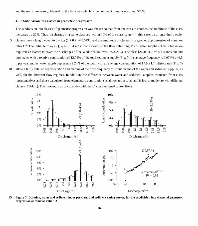
4.1.3 Subdivision into classes in geometric progression
The subdivision into classes of geometric progression was chosen so that from one class to another, the amplitude of the class
increases by 20%. Thus, discharges in a same class are within 10% of the class center. In this case, on a logarithmic scale,
classes have a length equal to β = log (1 + 0.2) ≅ 0.0792, and the amplitude of classes is in geometric progression of common 5
ratio 1.2. The initial term a0 = QR1% = 0.164 m3 s-1 corresponds to the flow delimiting 1% of water supplies. This subdivision
required 42 classes to cover the discharges of the Wadi Sebdou over 1973-2004. The class [26.4; 31.7 m3 s-1[ stands out and
dominates with a relative contribution of 12.74% of the total sediment supply (Fig. 7). Its average frequency is 0.074% or 6.5
h per year and its water supply represents 2.24% of the total, with an average concentration of 17.8 g L-1. Histograms (Fig. 7)
allow a fairly detailed representation and reading of the flow frequency distribution and of the water and sediment supplies, as 10
well, for the different flow regimes. In addition, the difference between water and sediment supplies estimated from class
representatives and those calculated from elementary contributions is almost nil in total, and is low to moderate with different
classes (Table 1). The maximum error coincides with the 1st class assigned to low flows.
Figure 7: Duration, water and sediment input per class, and sediment rating curves, for the subdivision into classes of geometric 15 progression of common ratio 1.2
(29,17.4 )
y = 0.5032x0.7917
R² = 0.95
0.01
0.1
1
10
100
0.01 0.1 1 10 100
Conce
ntr
atio
n g
L-1
Discharge m3s-1
29 (
2.2
4%
)
0%
3%
5%
8%
10%
0.0
8
0.3
6
0.9
1
2.3
5.6
14.0
34.8
86.6
216
Runoff
contr
ibuti
on
Discharge m3s-1
29 (
0.0
74%
)
0%
3%
6%
9%
12%
15%
0.0
8
0.3
6
0.9
1
2.3
5.6
14.0
34.8
86.6
216
Tim
e du
rati
on
Discharge m3s-1
29
(2
.24
%)
0%
3%
6%
9%
12%
15%
0.0
8
0.3
6
0.9
1
2.3
5.6
14.0
34.8
86.6
216
Sed
imen
t co
ntr
ibuti
on
Discharge m3s-1

17
The determination coefficient and Nash-Sutcliffe coefficient (1970) of the rating curve, Ck = a Qk b, are satisfactory for the
three types of subdivisions used in this study (Table 1). However, the best performances are obtained with the subdivision in
geometric progression which also allows a better quantification of the sediment supply (Table 1).
4.2 Return periods
The annual series of maximum flow rate series, QMAX, and half-load discharge, QY50, fit log-normal distributions (Fig. 8). 5
These two probability distributions make it possible to evaluate recurrence intervals related to QD values. The two subdivisions
with very close QD values (equal classes of amplitudes 1 m3 s-1 and in geometric progression of common ratio 1.2) give similar
recurrence intervals: the return periods of QD are 2.2 years for the annual series QMAX and 6.9 to 7 years for the annual series
QY50 (Table 2). The difference of nearly five years is attributed to their different meanings. While one indicates that the
effective discharge is observed at least once in a hydrological year roughly every two years at the gauging station, the other 10
shows that half of the yearly sediment supply is carried by flows higher than the effective discharge only every 7 hydrological
years.
Figure 8: Adjustment to the log-normal distribution of maximum annual discharges, QMAX, and median annual discharges, QY50.
15
Table 2: Recurrence intervals, R.I. QMAX and R.I. QY50, of the dominant discharge QD calculated for the subdivisions into classes of
equal amplitude 1 m3 s-1 and of geometric progression.
Method for QD calculation QD (m3 s-1) R.I. QMAX (year) R.I. QY50 (year)
subdivision into classes of equal length 1 m3 s-1 29.50 2.18 7.02
subdivision in geometric progression (1.2) 29.01 2.16 6.91
0%
20%
40%
60%
80%
100%
0 20 40 60 80 100
Annual median discharge QY50 (m3 s-1)
Empirical frequency
Log-normal frequency
0%
20%
40%
60%
80%
100%
0 50 100 150 200 250 300
Annual maximum discharge QMAX (m3 s-1)
Empirical frequency
Log-normal frequency

18
4.3 Analytical determination of the effective discharge
The analytical approach requires to build a probability density function f(Q) representing the distribution of flow frequencies
as well as a curve g(Q) representing the solid discharge QS as a function of the water flow Q. The study shows that these two
curves are closely related to the types of subdivisions used. For the subdivision into classes of equal amplitude 1 m3 s-1 and the
one with geometric progression of common ratio 1.2, the adjustment of flow frequency distribution to the log-normal and log-5
Gumbel probability distributions are satisfactory (Fig. 9), the log-Gumbel distribution showing to perform slightly best. The
highest difference for a class between the empirical and theoretical (log-Gumbel) frequency distributions was 4.1% for the
subdivision into classes of equal amplitudes and 4.8% for subdivision into geometric progression. Characteristic parameters
associated with the subdivision into classes of equal amplitudes and the one into geometric progression are (μ=-0.4148,
δ=0.6572) and (μ=-0.7180, δ=0.9649), respectively. However, the dominant discharges obtained when then log-Gumbel 10
distribution is considered are very low: QD=0.64 m3 s-1 for the subdivision into equal classes of amplitude 1 m3 s-1 (with b=
0.8031), and QD=0.62 m3 s-1 for the subdivision into geometric progression (with b=0.7917). The use of a log-normal
distribution leads to slightly higher values for QD: 0.92 m3 s-1 for the subdivision into classes of 1 m3 s-1 and 1.02 m3 s-1 for the
subdivision into geometric progression, far from the dominant discharges obtained from the histograms, 29.5 and 29.01 m3 s-
1 (Table 1). 15
Figure 9: Adjustment of the frequency distribution of flows to the log-Gumbel probability distribution: on the left, according to a
subdivision into equal classes of amplitudes 1 m3 s-1, and to the right, according to a subdivision into geometric progression of
common ratio 1.2.
50%
60%
70%
80%
90%
100%
1 10 100
Empirical frequency
Log-normal frequency
50%
60%
70%
80%
90%
100%
1 10 100
Discharge m3 s-1
Empirical frequency
Log-Gumbel frequency
0%
20%
40%
60%
80%
100%
0.1 1 10 100
Empirical frequency
Log-normal frequency
0%
20%
40%
60%
80%
100%
0.1 1 10 100
Discharge m3 s-1
Empirical frequency
Log-Gumbel frequency
19
5 Discussion
5.1 Pre-processing of data of the gauging station
Half-hour sampling carried out by the ANRH is unsuitable during the Wadi Sebdou flash floods, which produce more than
80% of the total sediment load in 1% of the time, with an estimated average concentration of 10.3 g L-1. To overcome the
presence of empty classes, Biedenharn et al. (2001), Goodwin (2004) and Crowder and Knapp (2005) propose to downgrade, 5
subjectively, the number of classes by readjusting their amplitude to cover all classes in information. Another alternative
applied in this study is to refine the dataset, by interpolation between measurements. The refinement tested in this study has
the advantage of not modifying the water and sediment budgets brought by the Wadi compared to the original series, since the
interpolation is linear. The discharge step chosen for the interpolation, close to the low flow at the hydrographic station, also
makes it possible to cover all classes of the different considered subdivisions and thus to make it possible to calculate the 10
effective discharge. Note that a similar method has already been applied by Biedenharn et al. (2001) and Gray et al. (2015) to
refined data from monthly step to daily steps, and by Simon et al. (2004) and Lenzi et al. (2006) from daily and hourly
measurements to a finer time step of 15 or even 5 minutes. In other studies, for which the frame of reference is the daily time
step, instantaneous measurements are replaced by daily averages (Andrews, 1980, Nolan et al., 1987, Emmett and Wolman,
2001). 15
5.2 Methodology to identify the dominant class in the mean approach
The quality of graphs and the error on water and sediment supplies made it possible to compare subdivisions and select those
that are able to represent the flows and to identify the effective discharge. Several studies dedicated to dominant discharge
class focused exclusively on the graphical aspect by readjusting the interval amplitude with equal classes until a dominant
class appears outside the first and last classes (Benson and Thomas, 1966; Pickup and Warner, 1976; Andrews, 1980; Hey, 20
1997; Lenzi et al., 2006; Roy and Sinha, 2014). However, this approach remains subjective (Sichingabula, 1999; Biedenharn
et al., 2001; Goodwin, 2004) and poses a dilemma. Reducing the class amplitude can make the dominant class emerge outside
the two extreme classes, but this can bring up empty classes which, conversely, require increasing the amplitude for each class
to be covered. Where appropriate, the series is considered non-compliant with the selection criteria and does not allow to
identify the dominant class (Crowder and Knapp, 2005). To avoid such situations, Bienderhan et al. (2000) recommended the 25
use of adequately provided datasets covering at least 10 years of measurements.
Yevjevich's (1972) proposal, based on statistical concepts, to use between 10 and 25 classes of amplitude less than s/4, where
s is the standard deviation of the flow series, is difficult to apply to the Wadi Sebdou. The standard deviation, which can be
calculated from 𝑠2 =1
𝑇∑ Δ𝑡𝑖(𝑄𝑖 − �̅�)2
𝑖 where �̅� =1
𝑇∑ Δ𝑡𝑖𝑄𝑖𝑖 and Δ𝑡𝑖 is the elementary time interval (Eq. 1), gives s/4 = 0.77
m3 s-1 for the Wadi Sebdou. Subdivision into classes of equal s/4 amplitudes would require 355 classes to cover the range of 30
flows. In a stream with such high flow variability, the strong flow asymmetry has a negative impact on the representativeness

20
of flows and sediment discharges, especially for low flow classes that cover most of the water supply. This suggestion does
not seem appropriate for wadis.
In this study, two types of subdivisions other than the classical subdivision with classes of equal amplitude were examined:
discharge classes corresponding to equal water supply, and a geometric progression of flows. The subdivisions into classes of
equal amplitude 1 m3 s-1 and the subdivision into classes with geometric progression best represented liquid and sediment 5
supplies (Table 1) and are used to characterize the Wadi Sebdou flows. They give dominant discharges (QD = 29.5 m3 s-1 and
QD = 29.0 m3 s-1, respectively) very close to each other and to the half-load discharge QY50 = 29.8 m3 s-1. This result is in
perfect agreement with Vogel et al. (2003). The half-load discharge, which is simple to compute, is used by several authors
(Doyle and Shields, 2008; Klonsky and Vogel, 2011; Ferro and Porto, 2012; Gray et al., 2015) and has been generalized to
identify the dominant discharge conveying various solid or dissolved matters (nutrients, sand, accidental pollution, etc.), 10
especially for the study of ecological aspects and environmental management (Vogel et al., 2003, Doyle et al., 2005,
Wheatcroft et al., 2010).
5.3 Limits to the use of a rating curve arid Qs=g(Q) in the Wadi Sebdou
The sediment supply calculated from data (ti, Qi, Ci) (reminder: the supply is the same with the 6,947 initial values as with the
40,081 values, linearly interpolated) provided a reference to evaluate the ability of a rating curve to estimate sediment 15
discharges from water flows. This rating curve g(Qk) = Qsk = a Qk (b+1) established from the series (Qk, Ck) generates errors we
call hereafter 'of the first type', which we must specify. The sediment supply associated to the kth discharge class is as follows:
∆Yk = 10−6g(Qk)∆TK (28)
where Qk and ∆TK are the center and the duration of flows corresponding to a given class.
On the Wadi Sebdou, despite a correct estimate of the total sediment supply for the two subdivisions of equal amplitude 1 m3 20
s-1 and in geometric progression (Figure 10, Table 1), the rating curve Qsk = a Qk (b+1) generates errors that induce a shift in the
class of dominant discharge (Figure 11). The subdivision into classes of equal amplitude leads to a value of effective discharge,
QD=1.5 m3 s-1, very low in comparison with the one calculated from initial data using eq. 5 (29.5 m3 s-1). The use of a rating
curve for Qs with the subdivision in geometric progression results in an effective discharge of 72.2 m3 s-1, well above the value
obtained directly (29.01 m3 s-1). These offsets are explained because the actual sediment discharges associated with each class 25
are around the rating curve g(Qk), sometimes below or sometimes above (Figs 4 and 7). For both subdivisions, the empirical
average sediment concentration observed in the dominant class is well above the rating curve. As a result, the rating curve
greatly underestimates the sediment supply in this class. Combined with the flow frequency, the supply is lowered compared
to other classes where the model overestimates the average concentration.
This result may be site-specific. Indeed, sediment-discharge rating curves fail to properly reproduce the dynamics of suspended 30
sediment flows in the Wadi Sebdou due to the hysteresis phenomena, studied in Megnounif et al. (2013). Such errors ‘of the
firt type’, high in the wadi Sebdou, may be reduced in other semiarid basins.

21
Figure 10: Comparison between the analytical sediment supply by class given from the rating curve (Qsk = a Qk (b+1), in ordinate)
and the elementary contributions 𝐐𝐒.𝐎𝐛𝐬 = 𝟏𝟎𝟔 ∆𝐘𝐊
∆𝐓𝐊 where ∆𝐘𝐊 (unit: 103 tonnes) and ∆𝐓𝐊 (unit: s) are obtained from Eq. 3 (in
abscissa): for a subdivision into classes of equal amplitudes 1 m3 s-1 (left) and with a geometric progression of common ratio 1.2
(right). 5
Figure 11: Sediment load histogram established using the sediment rating curve: for a subdivision into classes of equal amplitudes
1 m3 s-1 (left) and with a geometric progression of common ratio 1.2 (right).
5.4 Limits to the application of the analytical solution in semi-arid environments
When the flow frequency is represented by a probability distribution, the sediment load histogram can be built from this 10
distribution and the sediment rating curve. However, it should be remembered that for a continuous random variable such as
water discharge, the theoretical probability at a point does not exist in the probabilistic sense, but necessarily refers to an
interval. Thus, the contribution of a class, Ik, can be quantified by:
∆Yk = 10−6g(Q𝑘) [∫ 𝑓(𝑄)𝑑𝑄𝐼𝑘
] 𝑇 (29)
where Qk is the center of the Ik interval, f is the probability density function, and T is the total duration of the study period. 15
0
2000
4000
6000
8000
10000
12000
0 2000 4000 6000 8000 10000 12000
Theori
tical
sedim
ent
dis
charg
e k
g s
-1
Empirical sediment discharge kg s-1
0
2000
4000
6000
8000
10000
12000
0 2000 4000 6000 8000 10000 12000
Theori
tical
sedim
ent
dis
charg
e k
g s
-1
Empirical sediment discharge kg s-1
(29.0
, 5.6
%)
(72.2
, 8.8
%)
0%
2%
4%
6%
8%
10%
0,0
80,2
10,3
00,4
40,6
30,9
11,3
11,8
82,7
13,9
05,6
28,1
011
,716
,824
,234
,850
,172
,210
415
021
6
Sedim
ent
load c
ontr
ibution
Discharge m3s-1
(29.5
, 1.3
7%
)
0%
1%
2%
3%
4%
5%
0,5 30,5 60,5 90,5 120,5 150,5 180,5 210,5 240,5 270,5
Sedim
ent
load c
ontr
ibution
Discharge m3 s-1

22
Since the function f increases until the mode, Qmode, where it reaches its maximum, the dominant discharge QD is greater than
Qmode by construction (Fig. 1). The difference between QD and Qmode depends on the growth of the function g and the decrease
of the function f. However, for wadis, the scarcity of flood events and the dominance of low flows (80% of flows are less than
1 m3 s-1 on the Wadi Sebdou) require the use of a probability density function with a pronounced dissymmetry where, after the
mode, the decay is rapid. In this context, only the log-normal and log-Gumbel distributions have apparently shown a 5
satisfactory fit to subdivisions in classes of equal amplitude 1 m3 s-1 and in geometric progression (Fig. 9).
Figure 12: Analysis of errors (difference and ratio) between observed and theoretical frequencies of water discharge: for the log-
normal distribution (above) and for the log-Gumbel distribution (below).
However, the analysis of errors associated to the subdivision in geometric progression and the log-normal distribution (Figure 10
12) shows that above 18.3 m3 s-1, the ratio actual frequency on analytical frequency is very high and varies from 11.6 to more
than 105 for the log-normal distribution. Consequently, the analytic supply is minimal compared to the load calculated from
elementary contributions for these flows, and the total analytical supply given by Eq. 29 underestimates by 79% the sediment
supply established by Eq. 5. With the log-Gumbel distribution, the ratio varies between 0.16 and 1.69 and the total analytical
yield overestimates by 35% the one deduced from elementary contributions (Eq. 5). The offset is also high when flows are 15
subdivided into equal classes of amplitude 1 m3 s-1. Compared with the total analytical yield, low flow rates seem to be the
most effective. The class [1, 2 m3 s-1[ dominates with a contribution of about 6% for the log-normal distribution and 15.7% for
the log-Gumbel distribution. In this case, the total sediment load estimated from the log-normal and log-Gumbel distributions
underestimates by 84% and 66%, respectively, the empirical load. This example shows that the product of the theoretical
-6%
-4%
-2%
0%
2%
4%
6%
0.0
8
0.2
1
0.3
0
0.4
4
0.6
3
0.9
1
1.3
1
1.8
8
2.7
1
3.9
0
5.6
2
8.1
0
11.7
16.8
24.2
34.8
50.1
72.2
104
150
216
Dif
fere
nce
bet
wee
n e
mpir
ical
and
log-n
orm
al f
requen
cies
Discharge m3s-1
0.1
1
10
100
1000
10000
100000
1000000
0.0
8
0.2
1
0.3
0
0.4
4
0.6
3
0.9
1
1.3
1
1.8
8
2.7
1
3.9
0
5.6
2
8.1
0
11.7
16.8
24.2
34.8
50.1
72.2
104
150
216R
atio
bet
wee
n e
mpir
ical
and l
og
-
norm
al f
requen
cies
Discharge m3s-1
-6%
-4%
-2%
0%
2%
4%
6%
0.0
8
0.2
1
0.3
0
0.4
4
0.6
3
0.9
1
1.3
1
1.8
8
2.7
1
3.9
0
5.6
2
8.1
0
11.7
16.8
24.2
34.8
50.1
72.2
104
150
216
Dif
fere
nce
bet
wee
n e
mpir
ical
and
log-G
um
bel
fre
quen
cies
Discharge m3s-1
0.1
1
10
0.0
8
0.2
1
0.3
0
0.4
4
0.6
3
0.9
1
1.3
1
1.8
8
2.7
1
3.9
0
5.6
2
8.1
0
11.7
16.8
24.2
34.8
50.1
72.2
104
150
216R
atio
bet
wee
n e
mpir
ical
and l
og
-
Gum
bel
fre
quen
ccie
s
Discharge m3s-1
23
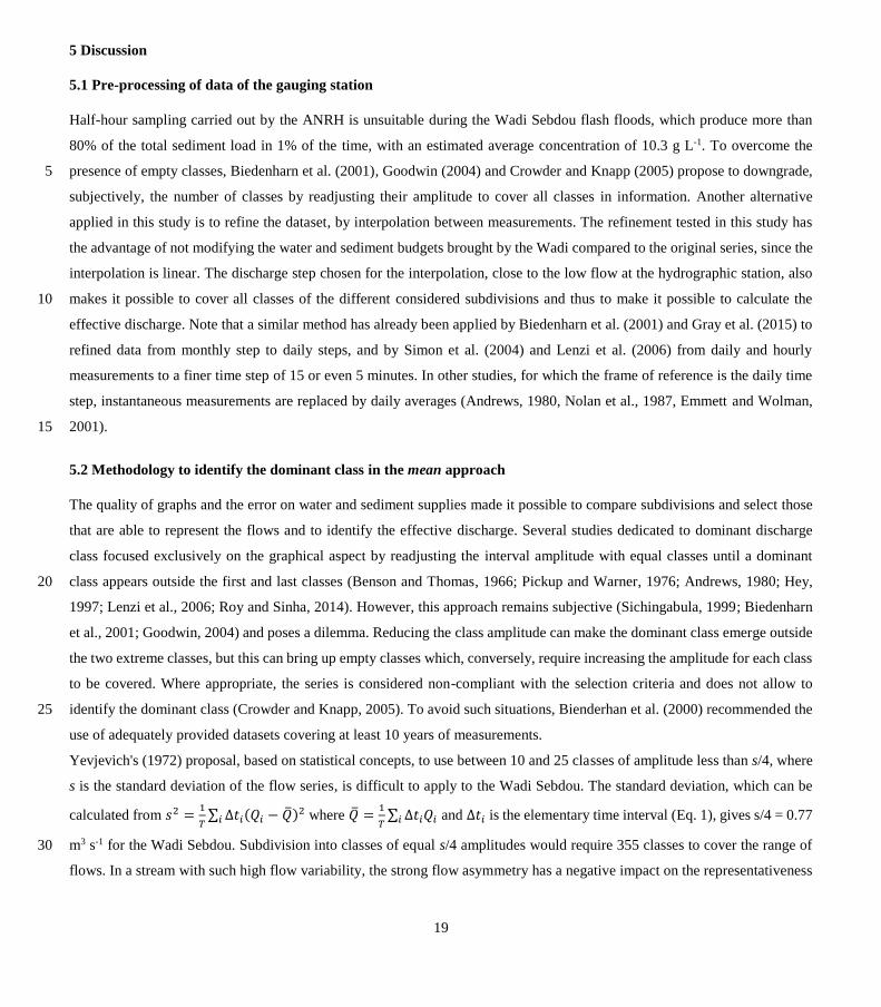
frequency distribution generates errors of a second type which are not taken into account in the construction of the sediment
load histogram which, as a result, poorly represents the distribution of the sediment supply (Fig. 13).This type of error may
likely be frequent in semi-arid environments, since the frequency of flash floods that carry high sediment supplies are not well
represented by pronounced asymmetric flow frequency distributions.
5
Figure 13: Three sediment load histograms obtained from the dataset, from the product of the rating curve times to the log-normal
distribution of discharges, and from the product of the rating curve times to the log-Gumbel distribution.
The analytical expressions giving QMode and QD (Eq.21, 22, 26 and 27) partly explain the low value of the dominant discharge
found for the Wadi Sebdou which is mainly dependent on the low value of the μ parameter due to the specific hydrologic
regime in semi-arid environments, where the annual modulus is very low, often below 1 m3 s-1. The dominant discharge is thus 10
very close to the mode. As a result, the analytical approach seems to be suitable only for rivers where extreme flows are less
distant from the mode than on wadis.
In summary, the pronounced asymmetric probability distributions which seemed to be adapted to the Wadi Sebdou failed to
reproduce good frequencies of high discharge associated to flash floods. Consequently, the mean method by decomposition of
histogram classes is the most suitable in a semi-arid environment. This had never been tested in the literature. It's an original 15
result of this paper.
Another point deserves a remark in the calculation of the effective discharge from f and g, for the general case. Whatever the
probability density function f, the sediment transport efficiency curve is given by h(Q) = a Q(b+1) f(Q). Thus, the effective
discharge, solution of the derived function h'(Q) = 0, is independent of the parameter a and depends only on the parameter b.
In other words, the dominant discharge depends exclusively on characteristics of the watercourse since parameter b is 20
commonly considered as an indicator of the erosive power of the watercourse (Leopold and Maddock, 1953; Roehl, 1962;
Fleming, 1969; Gregory and Walling, 1973; Robinson, 1977; Sarma, 1986; Reid and Frostick, 1987; Iadanza and Napolitano,
2006; Yang et al., 2007). However, the suspended sediment load in rivers is strongly influenced by characteristics of the basin
as well, where slopes contribution to sediment supply is high (Megnounif et al., 2013), and even sometimes higher than the
0%
2%
4%
6%
8%
10%
12%
14%
0.0
8
0.2
1
0.3
0
0.4
4
0.6
3
0.9
1
1.3
1
1.8
8
2.7
1
3.9
0
5.6
2
8.1
0
11
.7
16
.8
24
.2
34
.8
50
.1
72
.2
10
4
15
0
21
6
Sed
imen
t lo
ad c
ontr
ibuti
on
Discharge m3 s-1
Empirical Log-normal Log-Gumbel

24
one of the hydrographic network (Roehl, 1962; Gregory and Walling, 1973; Duysings, 1985; Asselman, 1999). The debate on
the relationship between a and b (see, e.g., Achite and Ouillon 2016) is still open.
Finally, it should be noted that introducing a density function necessarily gives a monomodal sediment transport efficiency
curve, whereas this is not necessarily the case. Pickup and Warner (1976), Carling (1988), Phillips (2002), Lenzi et al. (2006)
and Ma et al. (2010) reported the existence on some sites of a bimodal dominant flow. Hudson and Mossa (1997) pointed out 5
that sediment load histograms present a variety of forms, including bimodal and complex forms, that differ from the unimodal
form identified by Wolman and Miller (1960). In addition to the monomodal sediment load histograms, Ashmore and Day
(1988) distinguished three other kinds of histograms: bimodal, multimodal and complex. Of the 55 basins studied by Nash
(1994), 29 are bimodal and 9 are multimodal.
5.5 Sensitivity of the dominant class to the environment 10
Biedenharn et al. (2001) suggest to carefully study long (over 30 years) data series (liquid flow, sediment concentration, and
flow frequency) and to ensure that the hydrological regime of the watershed did not undergo a significant change in flow rates
or sediment production in the long term. Change can be attributed to climate change (Zhang and Nearing, 2005; Ziadat and
Taimeh, 2013; Liu et al., 2014; Achite and Ouillon 2016) or anthropogenic actions (Cerdà, 1998a, 1998b; Liu et al., 2014),
such as intensification of agriculture (Montgomery, 2007; Lieskovský and Kenderessy, 2013), deforestation (Walling, 2006), 15
forest fires (González-Pelayo et al., 2006; Cerdà et al. 2010) or urbanization (Graham et al., 2007; Whitney et al., 2015). In
the study area, and like North Africa and the Maghreb, there has been a continuous drought since the mid-1970s (Giorgi and
Lionello, 2008; Achite and Ouillon, 2016; Zeroual et al., 2016). Overall, decreasing rainfall is more concentrated over time
(Ghenim and Megnounif, 2016), which increases the susceptibility of soils to erosion (Shakesby et al., 2002; Bates et al., 2008;
Vachtman et al., 2012). Megnounif and Ghenim (2016) showed that sediment production, which is increasing with increasing 20
rainfall variability (Achite and Ouillon, 2007), increased significantly in the late 1980s, with a pivot in 1988. After 1988, the
annual sediment yield was on average 7 times higher compared to the previous period (Megnounif and Ghenim, 2013).
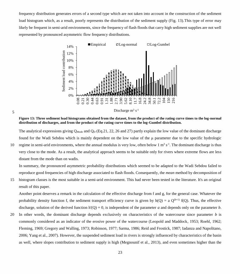
The application of a subdivision of discharge classes into geometric progression at the Wadi Sebdou for the two periods 1973-
1988 and 1988-2004 confirmed the change in the watershed functioning, with a bimodal sediment supply distribution for the
first period (Fig. 14). For 1973-1988, the class [6.1; 7.4 m3 s-1[, which includes the effective discharge QD = 6.7 m3 s-1, 25
contributed 7.5% of the total sediment yield. These relatively frequent flows last on average 0.5% of the annual time, i.e. 1.83
days, or 6.3% of the annual duration of floods which, for this period, lasted 7.65% of the annual time. The second peak was
observed for Q = 34.8 m3 s-1 representing the class [31.7; 38.0 m3 s-1[. Flows of this class were rare and lasted only 0.09% of
the annual time (7h45), but carried 5.9% of the total sediment yield. Over the period 1988-2004, the distribution of sediment
supply became essentially monomodal (Fig. 14) with a dominant flow QD = 29.0 m3 s-1. During this second period, an 30
increasing sediment contribution was also observed at high discharges (> 110 m3 s-1, up to 273 m3 s-1) that were not sampled
during the period 1973-1988.
25
Figure 14: Sediment supply by class for the subdivision in geometric progression: for 1973-1988 (left) and for 1988-2004 (right).
The half-load discharge in 1973-1988, QY50 (7.68 m3 s-1), was close to the dominant discharge QD (6.7 m3 s-1) and not far from
the modal class [6.1; 7.4 m3 s-1[; in 1988-2003, QY50 (31.80 m3 s-1) was very close to the modal class [26.4; 31.7 m3 s-1[ whose
center was defined as the effective discharge (QD = 29.0 m3 s-1). Thus, in the Sebdou Basin, the half-load discharge can be 5
seen as a robust proxy for the effective discharge. This result fosters further warrants in future studies and in other basins.
6 Conclusion
From a time series of flow and concentration data, a direct calculation provides estimates of water and sediment supplies by
summing the elementary contributions. This gives access to seasonal or annual values, and to the analysis of their variability.
Sediment dynamics can also be analyzed from discharge and sediment yield histograms by water discharge classes. On the 10
Wadi Sebdou, we have shown that an appropriate choice of subdivisions makes it possible to minimize the difference between
the flows estimated and measured at less than 10% (τY = τR = 8.8% for classes of equal amplitude 1 m3 s-1, Table 1) or even
less than 1% (τY = τR = 0.3% for classes in geometric progression of common ratio 1.2, Table 1). Classes thus defined make it
possible to determine a dominant class in the sense of sediment yield QD (29.5 or 29 m3 s-1 according to the two classifications
mentioned above) which is similar to the median flow in the sense of sediment yield QY50 (29.8 m3 s-1) on the Wadi Sebdou. 15
Other classifications have proved to be able to estimate the effective discharge (with a lesser precision) but unable to provide
good estimates of the water and sediment supplies (classes of equal amplitude greater than 1 m3 s-1), or able to estimate these
supplies but unable to estimate the effective discharge (classes with equal water supplies).
The introduction of a rating curve between the Qk and Ck series considered to build the histogram induced an additional bias
with respect to the direct calculation for the sedimentary yield. On the Wadi Sebdou, this bias, which depends on the choice 20
of subdivisions, can be reduced by 6 to 7% as indicated by τMY (Table 1), which is acceptable with regard to either the
uncertainties of measurements, or sometimes of inappropriate or insufficient sampling (Coynel et al., 2004). Previous work
(Megnounif et al., 2013) has shown the importance of hysteresis phenomena on this basin which induces a strong dispersion
29 (
14.2
%)
0%
3%
6%
9%
12%
15%
18%
0,0
8
0,2
5
0,4
4
0,7
6
1,3
2,3
3,9
6,7
11
,7
20
,1
34
,8
60
,2
10
4,0
17
9,6
Sedim
ent
contr
ibution
Discharge m3s-1
After September 1988
6.7
(7.5
%)
34.8
(5.9
%)
0%
3%
6%
9%
12%
15%
0,0
80,2
10,3
00,4
40,6
30,9
11,3
1,9
2,7
3,9
5,6
8,1
11
,716
,824
,234
,850
,172
,210
4,0
Sedim
ent
contr
ibution
Discharge m3s-1
Before September 1988

26
of instant parameter pairs (Q, C) and a bias in the estimation of supplies using a rating curve. The rating curve based on average
values by flow class, of defined length in geometric progression, appreciably improves statistical performances in the
computation of the sediment supply (higher value of R2, 0.95, and better Nash-Sutcliffe criterion, 0.93, compared to any other
method – see Table 1). It will be interesting in future works to analyze whether this is a singular phenomenon or whether the
use of a rating curve based on subdivision classes rather than on instantaneous measurements makes it possible to improve the 5
calculation of sediment yield compared with more conventional methods.
On the Wadi Sebdou, the coupled use of sediment rating a calibration curve and the log-normal and log-Gumbel probability
distributions were most likely to reproduce the observed regime, characterized by a very weak mode. However, they failed to
properly estimate the flow frequency of flash floods which are typical in semi-arid environments, and the corresponding
sediment yield. 10
Two return periods of the effective discharge were identified: one (from the annual maximum flow rate series, QMAX) for the
interval between two hydrological years with occurrence of the effective discharge, and one (from the QY50 annual half-load
discharge series) for the duration between two hydrologic years for which QY50 > QD, i.e. such than half of the sediment supply
at least is carried by flows higher than the effective discharge.
Flows of the dominant class carry the most sediment in the watercourse. It should be possible to link them to major processes 15
of erosion, transport and deposition that occur in the watershed. Lenzi et al. (2006), who have observed a bimodal sediment
contribution for a mountain river in the Alps in Italy, attributed the first modal class, of low but more frequent flow, to the
shaping of channel, and suggested that the second-class flows, larger in magnitude but of low occurrence, would be responsible
for the macroscale shape of the watercourse. On the Wadi Sebdou, we also observed a bimodal distribution. However, it is
difficult to conclude because the secondary mode of distribution obtained for the first period (1973-1988) became the dominant 20
mode of distribution later (1988-2004). The modes moved with the hydrological regime towards higher and higher sediment
yields, in line with what has been observed on most of watersheds studied over the last decades in the semi-arid environments
of Algeria (e.g. Achite and Ouillon, 2016). Applying this method to other watersheds will undoubtedly allow us to go further
in the analysis of dominant discharges and in their dynamics, in a context of global change.
References 25
Achite, M., and Ouillon, S.: Suspended sediment transport in a semiarid watershed, Wadi Abd, Algeria (1973-1995), J. Hydrol.,
343 (3-4), 187-202, doi:10.1016/j.jhydrol.2007.06.026, 2007.
Achite, M., and Ouillon, S.: Recent changes in climate, hydrology and sediment load in the Wadi Abd, Algeria (1970-2010).
Hydrol. Earth Syst. Sci., 20, 1355-1372, doi:10.5194/hess-20-1355-2016, 2016.
Alexandrov, Y., Laronne, J.B., and Reid, I.: Suspended sediment concentration and its variation with water discharge in a 30
dryland ephemeral channel, northern Negev, Israel, J. Arid Envir., 53, 73-84, doi:10.1006/jare.2002.1020, 2003.

27
Alexandrov, Y., Laronne, J.B., and Reid, I. Intra-event and inter-seasonal behaviour of suspended sediment in flash floods of
the semi-arid northern Negev, Israel. Geomorphology 85, 85-97, doi:10.1016/j.geomorph.2006.03.013, 2007.
Andrews E.D.: Effective and bankfull discharges of streams in the Yampa River basin, Colorado and Wyoming, J. Hydrol.,
46, 311-330, doi:10.1016/0022-1694(80)90084-0, 1980.
Ashmore, P.E., and Day, T.J.: Effective discharge for suspended sediment transport in streams of the Saskatchewan River 5
Basin. Water Resources Research 24 (6), 864–870, doi: 10.1029/WR024i006p00864, 1988.
Asselman, N.E.M.: Suspended sediment dynamics in a large drainage basin: the River Rhine. Hydrol. Proc. 13, 1437–1450,
doi: 10.1002/(SICI)1099-1085(199907)13:10<1437::AID-HYP821>3.0.CO;2-J, 1999.
Bagnold R.A.: The physics of blown sand and desert dunes. London, Methuen and Co, 1941.
Bates, B.C., Kundzewicz Z.W., Wu S., and Palutikof J.P., Eds.: Climate Change and Water. Technical Paper of the 10
Intergovernmental Panel on Climate Change, IPCC Secretariat, Geneva, 210 pp, 2008.
Benest, M.: Les formations carbonatées et les grands rythmes du Jurassique supérieur des monts de Tlemcen (Algérie). C.R.
Acad. Sci. Paris. Série D, t. 275, 1469-1471, 1972.
Benest, M., Elmi, S., and Bensalah, M.: Précisions stratigraphiques sur le Jurassique inférieur et moyen de la partie méridionale
des Monts de Tlemcen (Algérie). C.R. Symp. Société Géologie France, Fasc. 8, 295-296, 1999. 15
Benson, M.A., and Thomas, D.M.: A definition of dominant discharge, Bulletin of the International Association of Scientific
Hydrology, 11, 76–80, 1966.
Biedenharn, D. S., Thorne, C. R., Soar, P. J., Hey, R. D., and Watson, C.C.: Effective discharge calculation guide, Int. J.
Sediment Res., 16(4), 445-459, 2001.
Bouanani A.: Hydrologie, transport solide et modélisation. Etude de quelques sous bassins de la Tafna (NW Algérie). Ph.D. 20
Thesis, Tlemcen University, Algeria, 250p, 2004.
Bunte, K., Abt, S.R., Swingle, K.W., and Cenderelli, D.A.: Effective discharge in Rocky Mountain headwater streams. Journal
of Hydrology, 519, 2136–2147, doi:10.1016/j.jhydrol.2014.09.080, 2014.
Carling, P.A.: The concept of dominant discharge applied to two gravel-bed streams in relation to channel stability thresholds.
Earth Surface Processes and Landforms, 13, 355-367, 10.1002/esp.3290130407, 1988. 25
Castillo, V.M., Gomez-Plaza, A., and Martinez-Mena, M.: The role of antecedent soil water content in the runoff response of
semiarid catchments: a simulation approach. Journal of Hydrology, 284, 114-130, 10.1016/S0022-1694(03)00264-6, 2003.
Cerdà, A.: Relationships between climate and soil hydrological and erosional characteristics along climatic gradients in
Mediterranean limestone areas, Geomorphology, 25, 123-134, doi: 10.1016/S0169-555X(98)00033-6, 1998a.
Cerdà, A.: Effect of climate on surface flow along a climatological gradient in Israel. A field rainfall simulation approach. 30
Journal of Arid Environments, 38, 145-159, doi: 10.1006/jare.1997.0342, 1998b.
Cerdà, A., Lavee, H., Romero-Díaz, A., Hooke, J., and Montanarella, L.: Soil erosion and degradation in mediterranean type
ecosystems. Land Degradation and Development, 21(2), 71-74, doi:10.1002/ldr.968, 2010.
Chow, V. T., Maidment, D. R., and Mays, L. W.: Applied Hydrology. McGraw-Hill, New York, USA, 1988.

28
Colombani, J., Olivry, J.C., and Kallel, R.: Phénomènes exceptionnels d’érosion et de transport solide en Afrique aride et semi-
aride, Challenges in African Hydrology and Water Ressources. IAHS Publication, 144, 295–300, 1984.
Coynel, A., Schäfer, J., Hurtrez, J.E., Dumas, J., Etcheber, H., and Blanc, G.: Sampling frequency and accuracy of SPM flux
estimates in two contrasted drainage basins, The Science of the Total Environment 330, 233-247, doi:
10.1016/j.scitotenv.2004.04.003, 2004. 5
Crowder, D.W., and Knapp, H.V.: Effective discharge recurrence intervals of Illinois streams, Geomorphology, 64, 167-184,
doi: 10.1016/j.geomorph.2004.06.006, 2005.
Doyle, M. W., and Shields, C. A.: An alternative measure of discharge effectiveness. Earth Surface Processes Landforms, 33,
308–316, doi: 10.1002/esp.1543, 2008.
Doyle, M.W., Stanley E.H., Strayer D.L., Jacobson R.B., and Schmidt J.C.: Effective discharge analysis of ecological 10
processes in streams. Water Resources Research, 41, W11411, doi:10.1029/2005WR004222, 2005.
Dunne, T., and Leopold, L.B.: Water in Environmental Planning. W.H. Freeman, San Francisco, USA. 818 pp., 1978.
Duysing, J.J.H.M.: Streambank contribution to the sediment budget of forest stream. Unpubl. Ph.D. Thesis, Lab. Phys. Geogr.
Soil Sci., Univ. Amsterdam, 190 p., 1985.
Emmett, W.W., and Wolman, M.G. Effective discharge and gravel-bed rivers. Earth Surface Processes and Landforms 26, 15
1369–1380, 10.1002/esp.303, 2001.
Ferro V., and Porto P.: Identifying a dominant discharge for natural rivers in southern Italy, Geomorphology, 139-140, 313–
321, doi: 10.1016/j.geomorph.2011.10.035, 2012.
Fleming G.: Design curves for suspended load estimation. Proc. Inst. Civ. Ing., 43, 1-9, 1963.
Gao, P., and Josefson, M.: Temporal variations of suspended sediment transport in Oneida Creek watershed, central New York, 20
Journal of Hydrology, 426-427, 17-27. doi:10.1016/j.jhydrol.2012.01.012, 2012.
Ghenim, A.N., and Megnounif, A.: Variability and Trend of Annual Maximum Daily Rainfall in Northern Algeria,
International Journal of Geophysics, Article ID 6820397, doi:10.1155/2016/6820397, 2016.
Giorgi, F., and Lionello, P.: Climate change projections for the Mediterranean region. Global and Planetary Change, 63(2-3),
90-104, doi: 10.1016/j.gloplacha.2007.09.005, 2008. 25
González-Pelayo, O., Andreu, V., Campo, J., Gimeno-García, E., and Rubio, J.L.: Hydrological properties of a Mediterranean
soil burned with different fire intensities, Catena, 68, 186-193, 10.1016/j.catena.2006.04.006, 2006.
Goodwin, P.: Analytical solutions for estimating effective discharge, Journal of Hydraulic Engineering, 130, 729–738, doi:
10.1061/(ASCE)0733-9429(2004)130:8(729), 2004.
Graham, L. P., Andréasson, J., and Carlsson, B.: Assessing climate change impacts on hydrology from an ensemble of regional 30
climate models, model scales and linking methods–a case study on the Lule River basin. Climatic Change, 81(1), 293-307,
doi: 10.1007/s10584-006-9215-2, 2007.

29
Gray, A.B., Pasternack, G.B., Watson, E.B., Warrick, J.A., and Goñi, M.A.: Effects of antecedent hydrologic conditions, time
dependence, and climate cycles on the suspended sediment load of the Salinas River, California, Journal of Hydrology, 525,
632-649, 10.1016/j.jhydrol.2015.04.025, 2015.
Gregory, K.J., and Walling, D.E.: Drainage Basin Form and Process. Edward Arnold, London, 458 p., 1973.
Heusch, B.: Etude de l’érosion et des transports solides en zone semi-aride. Recherche bibliographique sur l’Afrique du Nord. 5
Projet RAB/80/04/PNUD, 1982.
Hey, R.D.: Channel response and channel forming discharge: literature review and interpretation, Final Report, U.S. Army
Contract Number R&D 6871-EN-01, 1997.
Higgins, A., Restrepo, J.C., Ortiz, J.C., Pierini, J., and Otero, L.: Suspended sediment transport in the Magdalena River
(Colombia, south America): Hydrologic regime, rating Parameters and effective discharge variability, International Journal of 10
Sediment Research, 31(1), 125-35, doi: 10.1016/j.ijsrc.2015.04.003, 2015.
Horowitz, A.J.: An evaluation of sediment rating curves for estimating suspended sediment concentrations for subsequent flux
calculations, Hydrological Processes, 17, 3387-3409, doi: 10.1002/hyp.1299, 2003.
Hudson, P.F., and Mossa, J.: Suspended sediment transport effectiveness of three large impounded rivers, U.S. Gulf Coast
Plain. Environ. Geol., 32, 263–273, doi: 10.1007/s002540050216, 1997. 15
Iadanza, C., and Napolitano, F.: Sediment transport time series in the Tiber River, Physics Chem. Earth, 31, 1212-1227, doi:
10.1016/j.pce.2006.05.005, 2006.
Klonsky, L., and Vogel, R.M.: Effective Measures of “Effective” Discharge, The Journal of Geology, 119, 1-14. doi:
10.1086/657258, 2011.
Lenzi, M.A., Mao, L., and Comiti, F.: Effective discharge for sediment transport in a mountain river: Computational 20
approaches and geomorphic effectiveness, Journal of Hydrology 326, 257-276, doi: 10.1016/j.jhydrol.2005.10.031, 2006.
Leopold, L.B., and Maddock, T.Jr.: The Hydraulic Geometry of Stream Channels and Some Physiographic Implications, U.S.
Geological Survey, Professional Paper 252, 56 p, 1953.
Lieskovský, J., and Kenderessy, P.: Modelling the effect of vegetation cover and different tillage practices on soil erosion in
vineyards: a case study en Vráble (Slovakia) using WATEM/SEDEM. Land Degradation and Development, 25, 288-296, doi: 25
10.1002/ldr.2162.2014, 2014.
Liu, Z., Yao, Z., Huang, H., Wu, S. and Liu, G.: Land use and climate changes and their impacts in the Yarlung Zangbo river
basin, China. Land Degradation and Development, 25, 203–215, doi: 10.1002/ldr.1159, 2014.
Ma, Y.X., Huang, H.Q., Xu, J.X., Brierley, G.J., Yao, Z.J.: Variability of effective discharge for suspended sediment transport
in a large semi-arid river basin, Journal of Hydrology, 388, 357-369, doi: 10.1016/j.jhydrol.2010.05.014, 2010. 30
Malina, F.J.: Recent developments in the dynamics of wind-erosion, Am. Geophys. Union Trans. pt 2, 262-287, 1941.
McKee, L.J., Hossain, S., and Eyre, B.D.: Magnitude-frequency analysis of suspended sediment loads in the subtropical
Richmond River basin, northern New South Wales, Australia. IAHR Publication 276, 289-296, 2002.
30
Megnounif, A., and Ghenim, A.N.: Influence des fluctuations hydropluviométriques sur la production des sédiments : Cas du
bassin de la haute Tafna. Rev Sci Eau 26(1):53–62. doi:10.7202/1014919ar, 2013.
Megnounif A., and Ghenim A.N.: Rainfall irregularity and its impact on the sediment yield in Wadi Sebdou watershed, Algeria,
Arab J Geosci (2016) 9:267, doi:10.1007/s12517-015-2280-y, 2016.
Megnounif, A., Terfous, A., Ouillon, S.: A graphical method to study suspended sediment dynamics during flood events in the 5
Wadi Sebdou, NW Algeria (1973-2004), J. Hydrology, 497, 24-36, doi:10.1016/j.jhydrol.2013.05.029, 2013.
Megnounif, A., Terfous, A., and Bouanani, A.: Production and transport of suspended sediment transport in the Upper-Tafna
river basin (North West Algeria). Rev. Sci. Eau 16 (3), 369-380, 2003.
Milliman, J.D., and Syvitski, J.P.M.: Geomorphic/tectonic control of sediment discharge to the ocean: the importance of small
mountainous rivers. J. Geology 100, 325-344, doi: 10.1086/629606, 1992. 10
Montgomery, D.R.: Soil erosion and agricultural sustainability. Proc Nat. Acad Sci, 04(13), 268-272, doi:
10.1073/pnas.0611508104, 2007.
Nash, D.B.: Effective sediment-transporting discharge from magnitude-frequency analysis. Journal of Geology 102, 79–95,
doi: 10.1086/629649, 1994.
Nash, J.E., and Sutcliffe, J.V.: River flow forecasting through conceptual models, Part I—A discussion of principles. J. 15
Hydrol., 10, 282–290, doi:10.1016/0022-1694(70)90255-6, 1970.
Nolan, K.M., Lisle, T.E., and Kelsey, H.M.: Bankfull discharge and sediment transport in northwestern California. Erosion
and sedimentation in the Pacific Rim. IAHS Publication 165, 439-449, 1987.
Phillips, J.D.: Geomorphic impacts of flash flooding in a forested headwater basin, J. Hydrol., 269:236-250, doi:
10.1016/S0022-1694(02)00280-9, 2002. 20
Pickup, G., and Warner, R.F.: Effects of hydrologic regime on magnitude and frequency of dominant discharge. Journal of
Hydrology 29, 51-75, doi: 10.1016/0022-1694(76)90005-6, 1976.
Probst, J.L., and Amiotte-Suchet, P.A.: Fluvial suspended sediment transport and mechanical erosion in the Maghreb (North
Africa), Hydrological Sciences Journal, 37(6), 621-637, doi: 10.1080/02626669209492628, 1992.
Quader, A., Guo, Y., and Stedinger, J.R.: Analytical estimation of effective discharge for small southern Ontario streams. Can. 25
J. Civ. Eng., 35, 1414-1426, doi:10.1139/L08-088, 2008.
Reid, I., Frostick, L.E.: Discussion of conceptual models of sediment transport in streams. In: Thorne CR, Bathurst JC, Hey
RD (eds), Sediment transport in gravel-bed rivers. Wiley, New York, 410-411, 1987.
Reid, I., and Laronne, J.B.: Bed load sediment transport in an ephemeral stream and a comparison with seasonal and perennial
counterparts. Water Resources Research 31 (3), 773-781, doi: 10.1029/94WR02233, 1995. 30
Robinson, A.R.: Relationships between soil erosion and sediment delivery. Erosion and Solid Matter Transport in Inland
Waters, IAHS Bull. 122, 159-167, 1977.
Roehl, J.W.: Sediment source areas, delivery ratios, and influencing morphological factors, IAHS Publication 59, 202–213,
1962.

31
Roy, N.G., and Sinha, R.: Effective discharge for suspended sediment transport of the Ganga River and its geomorphic
implication, Geomorphology, 227, 18-30, doi: 10.1016/j.geomorph.2014.04.029, 2014.
Sarma, J.N.: Sediment transport in the Burhi Dihing River, India. In: Hadley RF (Ed) Drainage basin sediment delivery, IAHS
Publ., 159, 199-215, 1986.
Scott, S.: Predicting sediment transport dynamics in ephemeral channels: a review of literature. ERDC/CHL CHETN-VII-6. 5
U.S. Army Engineer Research and Development Center, Vicksburg, http://chl.erdc.usace.army.mil/chetn, 2006.
Shakesby, R.A., Coelho, C.O.A., Schnabel, S., Keizer, J.J., Clarke, M.A., Lavado Contador, J.F., Walsh, R.P.D., Ferreira,
A.J.D., and Doerr, S.H.: A ranking methodology for assessing relative erosion risk and its application to dehesas and montados
in Spain and Portugal, Land Degrad Dev, 13, 129-140, doi: 10.1002/ldr.488, 2002.
Shields A., 1936. Anwendung der Ähnlichkeitsmechnik und der Turbulenz Firschung auf die geschiebebewegung Mitt, Der 10
Preuss. Versuchsamst. für Wasserbau und Schiffbau, Heft 26, Berlin, Deutschland, 1936.
Sichingabula, H.M.: Magnitude-frequency characteristics of effective discharge for suspended sediment transport, Fraser
River, British Columbia, Canada, Hydrological Processes, 13, 1361-1380, doi: 10.1002/(SICI)1099-
1085(19990630)13:9<1361::AID-HYP808>3.0.CO;2-H, 1999.
Simon, A., Dickerson, W., and Heins, A.: Suspended-sediment transport rates at the 1.5-year recurrence interval for ecoregions 15
of the United States: transport conditions at the bankfull and effective discharge, Geomorphology 58, 243–262,
doi:10.1016/j.geomorph.2003.07.003, 2004.
Terfous, A., Megnounif, A., and Bouanani, A.: Etude du transport solide en suspension dans l’Oued Mouilah (Nord-Ouest
Algérien). Revue Sciences de l’Eau, 14 (2), 173-185, 2001.
Vachtman, D., Sandler, A., Herut, B., and Greenbaum, N.: Dynamics of suspended sediment delivery to the Eastern 20
Mediterranean continental shelf, Hydrological Processes, doi: 10.1002/hyp.9265, 2012.
van Rijn, L.C.: Principles of sediment transport in rivers, estuaries and coastal seas. Aqua publications, 2005.
Vogel, R.M., Stedinger J.R., and Hooper R.P.: Discharge indices for water quality loads, Water Resources Research, 39 (10),
1273, doi:10.1029/2002WR001872, 2003.
Walling, D.E.: The impact of global change on erosion and sediment dynamics: current progress and future challenges, 25
UNESCO-IHP International Sediment Initiative (ISI) paper (downloadable at
http://unesdoc.unesco.org/images/0018/001850/185078E.pdf), 2008.
Walling, D.E.: Human impact on land–ocean sediment transfer by the world’s rivers. Geomorphology 79:192–216.
doi:10.1016/j.geomorph.2006.06.019, 2006.
Walling, D.E.: Derivation of erosion and sediment yield parameters in areas with deficient data reconnaissance measurements. 30
Hydrological Sciences - Bulletin des Sciences Hydrologiques, XXII, 4 12/197, 517-520, 1977.
Watson, C.C., Biedenharn, D.S., and Thorne, C.R. (Eds.): Demonstration Erosion Control: Design Manual. Engineer Research
and Development Center. U.S. Army Corps of Engineering, Engineer Research and Development Center, Vicksburg, MS. 274
pp., 1999.

32
West, T.S., and Niezgoda, S.L.: Estimating a stream restoration design discharge. Proceedings of the World Environmental
and Water Resource Congress: Examining the Confluence of Environmental and Water Concerns, ASCE, 2006.
Wheatcroft, R.A., Goñi, M.A., Hatten, J.A., Pasternack, G.B., and Warrick, J.A.: The role of effective discharge in the ocean
delivery of particulate organic carbon by small, mountainous river systems. Limnol. Oceanogr., 55(1), 161–171, doi:
10.4319/lo.2010.55.1.0161, 2010 5
Whitney, J.W., Glancy, P.A., Buckingham, S.E., and Ehrenberg, A.C.: Effects of rapid urbanization on streamflow, erosion,
and sedimentation in a desert stream in the American Southwest, Anthropocene, 10, 29-42, doi: 10.1016/j.ancene.2015.09.002,
2015.
Wolman, M.G., and Miller, J.P.: Magnitude and frequency of forces in geomorphic processes, Journal of Geology 68, 54-74,
1960. 10
Yang, G.F., Chen, Z.Y., Yu, F.L., Wang, Z.H., and Zhao, Y.W.: Sediment rating parameters and their implications: Yangtze
River, China. Geomorphology 85:166–175. doi:10.1016/j.geomorph.2006.03.016, 2007.
Yevjevich, V.: Probability and Statistics in Hydrology, Water Resources Publications, Fort Collins, USA, Colorado, 302 pp.,
1972.
Zeroual, A., Assani, A.A., and Meddi, M.: Combined analysis of temperature and rainfall variability as they relate to climate 15
indices in Northern Algeria over the 1972-2013 period, Hydrology Research, 48(2), 584-595. doi: 10.2166/nh.2016.244, 2016.
Zhang, X.C., and Nearing, M.A.: Impact of climate change on soil erosion, runoff, and wheat productivity in central Oklahoma,
Catena, 61(2), 185-195, doi: 10.1016/j.catena.2005.03.009, 2005.
Ziadat, F.M., and Taimeh A.Y.: Effect of rainfall intensity, slope and land use and antecedent soil moisture on soil erosion in
an arid environment. Land Degradation & Development, 24: 582- 590. doi: 10.1002/ldr.2239, 2013. 20