ME451 Kinematics and Dynamics

of Machine Systems

Basic Concepts in Planar Kinematics - 3.1

Absolute Kinematic Constraints – 3.2

Relative Kinematic Constraints – 3.3

September 29, 2011

© Dan Negrut, 2011ME451, UW-Madison

“There is no reason for any individual to have a computer in their home.”Ken Olson, president and founder, Digital Equipment Corporation, 1977.

Before we get started…

Last time: Computing the velocity and acceleration of a point attached to a moving rigid body Absolute vs. relative generalized coordinates Start Chapter 3: Kinematics Analysis

Today: Wrap up high level discussion of Kinematics Analysis after introducing the concept of

Jacobian Start discussion on how to formulate Kinematic constraints associated with a mechanism

Absolute kinematic constraints Relative kinematic constraints

Assignment 4 due one week from today: Problems 2.6.1, 3.1.1, 3.1.2, 3.1.3 ADAMS and MATLAB components emailed to you

Assignment 3 due today Problems due in class MATLAB and ADAMS part due at 23:59 PM 2

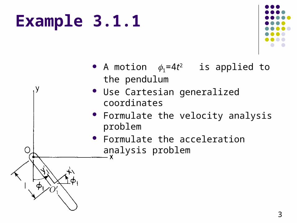
Example 3.1.1

A motion 1=4t2 is applied to the pendulum Use Cartesian generalized coordinates Formulate the velocity analysis problem Formulate the acceleration analysis problem

3

Kinematic Analysis Stages Position Analysis Stage

Challenging

Velocity Analysis Stage Simple

Acceleration Analysis Stage OK

4

To take care of all these stages, ONE step is critical: Write down the constraint equations associated with the joints

present in your mechanism Once you have the constraints, the rest is boilerplate

Once you have the constraints…(Going beyond the critical step)

5

The three stages of Kinematics Analysis: position analysis, velocity analysis, and acceleration analysis they each follow *very* similar recipes for finding for each body of the mechanism its position, velocity and acceleration, respectively

ALL STAGES RELY ON THE CONCEPT OF JACOBIAN MATRIX: q – the partial derivative of the constraints wrt the generalized coordinates

ALL STAGES REQUIRE THE SOLUTION OF A SYSTEM OF EQUATIONS

WHAT IS DIFFERENT BETWEEN THE THREE STAGES IS THE EXPRESSION OF THE RIGHT-SIDE OF THE LINEAR EQUATION, “b”

The Details…

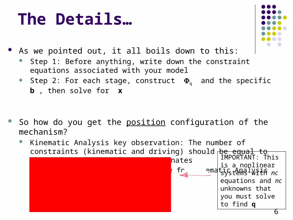
As we pointed out, it all boils down to this: Step 1: Before anything, write down the constraint equations associated with

your model Step 2: For each stage, construct q and the specific b , then solve for x

So how do you get the position configuration of the mechanism? Kinematic Analysis key observation: The number of constraints (kinematic

and driving) should be equal to the number of generalized coordinates This is, NDOF=0, a prerequisite for Kinematic Analysis

6

IMPORTANT: This is a nonlinear systems with nc equations and nc unknowns that you must solve to find q

Getting the Velocity and Acceleration of the Mechanism

Previous slide taught us how to find the positions q At each time step tk, generalized coordinates qk are the solution of a nonlinear system

Take one time derivative of constraints (q,t) to obtain the velocity equation:

Take yet one more time derivative to obtain the acceleration equation:

NOTE: Getting right-hand side of acceleration equation is tedious

7

Producing RHS of Acceleration Eq.[In light of previous example]

RHS was shown to be computed as

Note that the RHS contains (is made up of) everything that does *not* depend on the generalized accelerations

Implication: When doing small examples in class, don’t bother to compute the RHS using

expression above This is done only in ADAMS, when you shoot for a uniform approach to all problems

Simply take two time derivatives of your simple constraints and move everything that does *not* depend on acceleration to the RHS

8

[What comes next:]

Focus on Geometric Constraints

Learn how to write kinematic constraints that specify that the location and/or attitude of a body wrt the global (or absolute) RF is constrained in a certain way Sometimes called absolute constraints

Learn how to write kinematic constraints that couple the relative motion of two bodies Sometimes called relative constraints

9

The Drill…[related to assignment]

Step 1: Identify a kinematic constraint (revolute, translational, relative distance, etc., i.e., the physical thing) acting between two components of a mechanism

Step 2: Formulate the algebraic equations that capture that constraint, (q)=0 This is called “modeling”

Step 3: Compute the Jacobian (or the sensitivity matrix) q

Step 4: Compute , the right side of the velocity equation

Step 5: Compute , the right side of the acceleration equation (ugly…)

10This is what we do almost exclusively in Chapter 3 (about two weeks)

Absolute Constraints

Called “Absolute” since they express constraint between a body in a system and an absolute (ground) reference frame

Types of Absolute Constraints

Absolute position constraints

Absolute orientation constraints

Absolute distance constraints

11

Absolute Constraints (Cntd.)

Absolute position constraints x-coordinate of Pi

y-coordinate of Pi

Absolute orientation constraint Orientation f of body

12

Body “i”

Absolute x-constraint Step 1: the absolute x component of the location of a

point Pi in an absolute (or global) reference frame stays constant, and equal to some known value C1

13

Step 2: Identify ax(i)=0

Step 3: ax(i)q = ?

Step 4: ax(i) = ?

Step 5: ax(i) = ?

NOTE: The same approach is used to get the y- and angle-constraints

Absolute distance-constraint

Step 1: the distance from a point Pi to an absolute (or global) reference frame stays constant, and equal to some known value C4

14

Step 2: Identify dx(i)=0

Step 3: dx(i)q = ?

Step 4: dx(i) = ?

Step 5: dx(i) = ?