1

ME 233 Advanced Control II

Lecture 3

Introduction to Probability Theory

(ME233 Class Notes pp. PR1-PR3)

2

Outline

• Continuous random variable

• CDF, PDF, expectation and variance

• Uniform and normal PDFs

Continuous random variable

A continuous-valued random X variable takes

on a range of real values

Example:

• An experiment whose outcome is a real

number, e.g. measurement of a noisy

voltage.

3

min max[ , ]X V V

• For the probability space,

• A random variable X is a mapping

4

Cumulative Distribution Function

Cumulative distribution function (CDF) associated

with the random variable X :

The probability that the random variable X

will be less than or equal to the value x

5

Properties of the cumulative distribution

0

1

a

6

Properties of the cumulative distribution

1.

2.

3. is a monotone non decreasing

4. is left-continuous

7

Probability Density Function

For a differentiable cumulative distribution function,

Define the probability density function (PDF),

8

Probability Density Function

Interpretation:

for small

Loosely interpret this as the probability that X takes

a value close to x

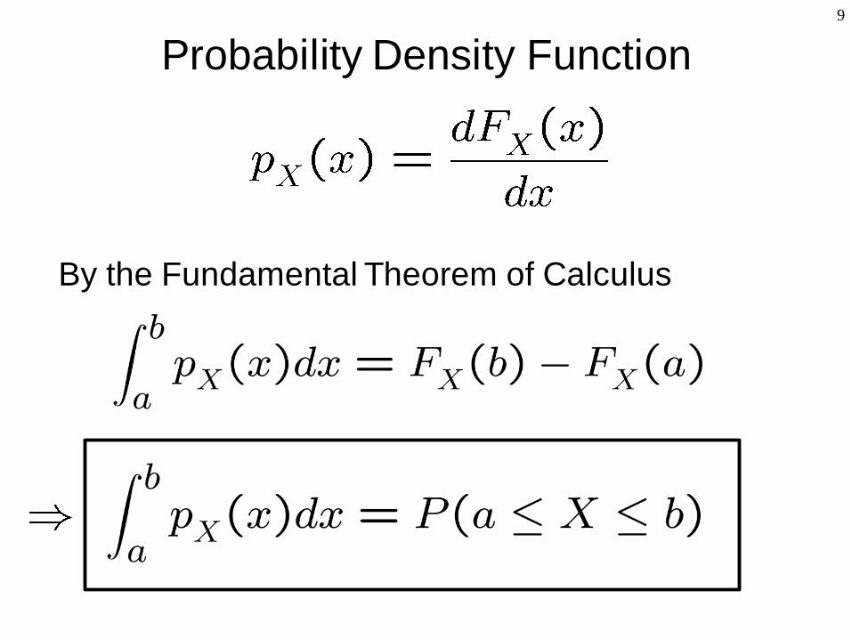
9

Probability Density Function

By the Fundamental Theorem of Calculus

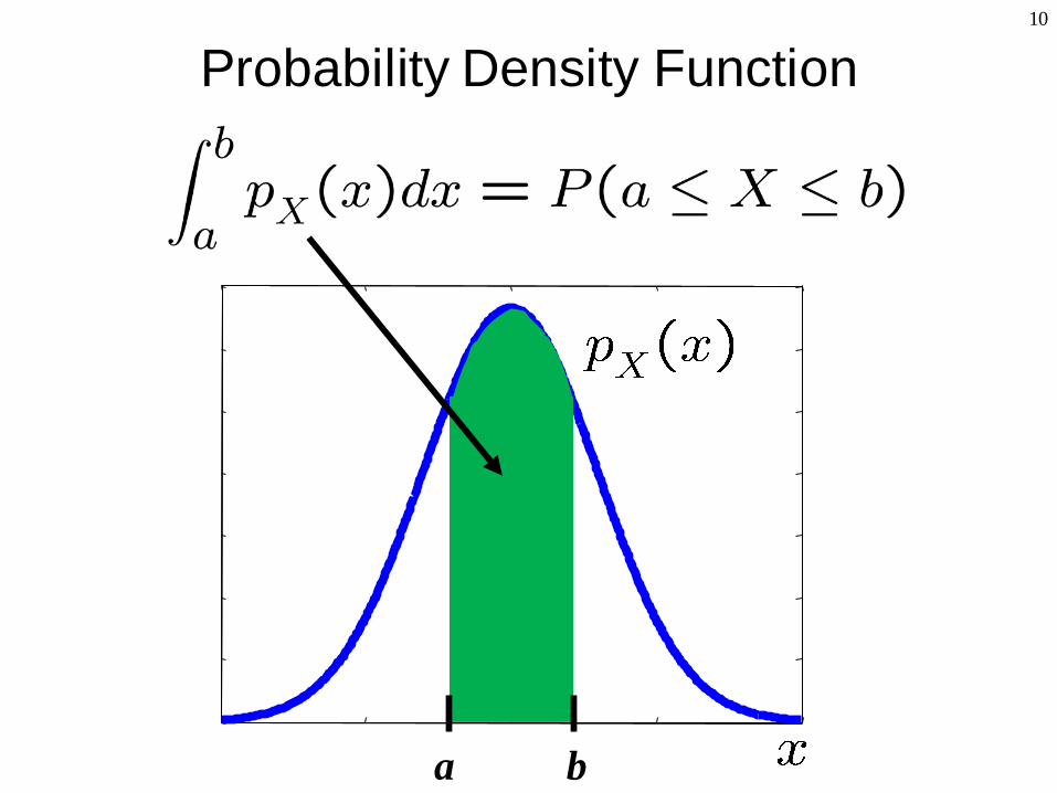
10

Probability Density Function

a b

11

Probability Density Function

Property:

because

12

Expectation

The expected value of random variable X is:

This is the average value of X.

It is also called the mean of X

or the first moment of X

13

Expected value - notation

14

Expected value of a function

f : real valued function of random variable X

The expected value of Y is

15

Variance

The variance of random variable X is:

where

Is called the standard deviation of X

16

Variance

where

17

Proof

18

Uniform Distribution

A random variable X which is uniformly distributed

between xmin and xmax has the PDF:

xmin xmaxx

xmin

xmax

1

p (x)X matlab function: rand

Summing independent uniformly distributed random

variables

• Let X and Y be 2 independent uniformly

distributed variables between [0,1]

• The random variable

• is not uniformly distributed

19

Z X Y

Summing independent uniformly distributed random

variables

• Let X and Y be 2 independent uniformly

distributed variables between [0,1]

20

Z X Y

X=rand(1,1e5);

Y=rand(1,1e5);

Z=X+Y;

[freqZ,cent]=hist(Z,100);

bin_width=(cent(100)-cent(1))/99;

area = sum(freqZ)*bin_width;

bar(centers,freqZ/area)

xlabel('z')

ylabel('F_Z(z)')

105 random

samples of Z

Histogram of

Z with

normalized

area

Summing independent uniformly distributed random

variables

• Let X and Y be 2 independent uniformly

distributed variables between [0,1]

21

Z X Y

z

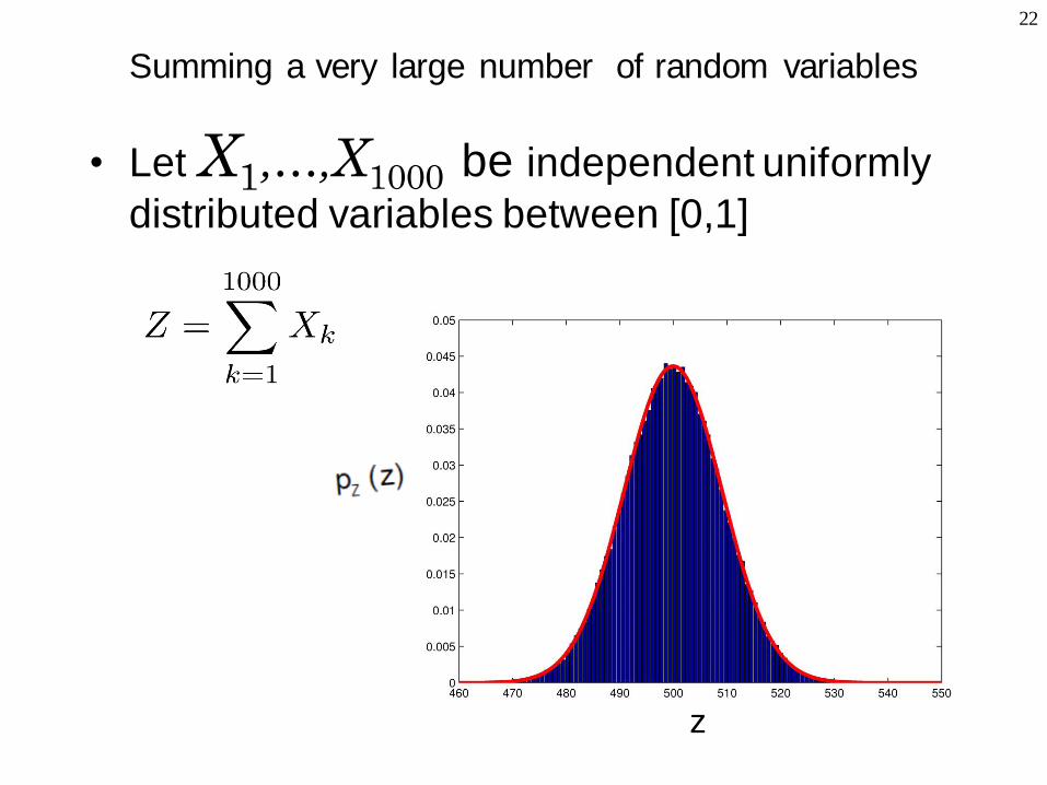
• Let X1,…,X1000 be independent uniformly

distributed variables between [0,1]

Summing a very large number of random variables

22

z

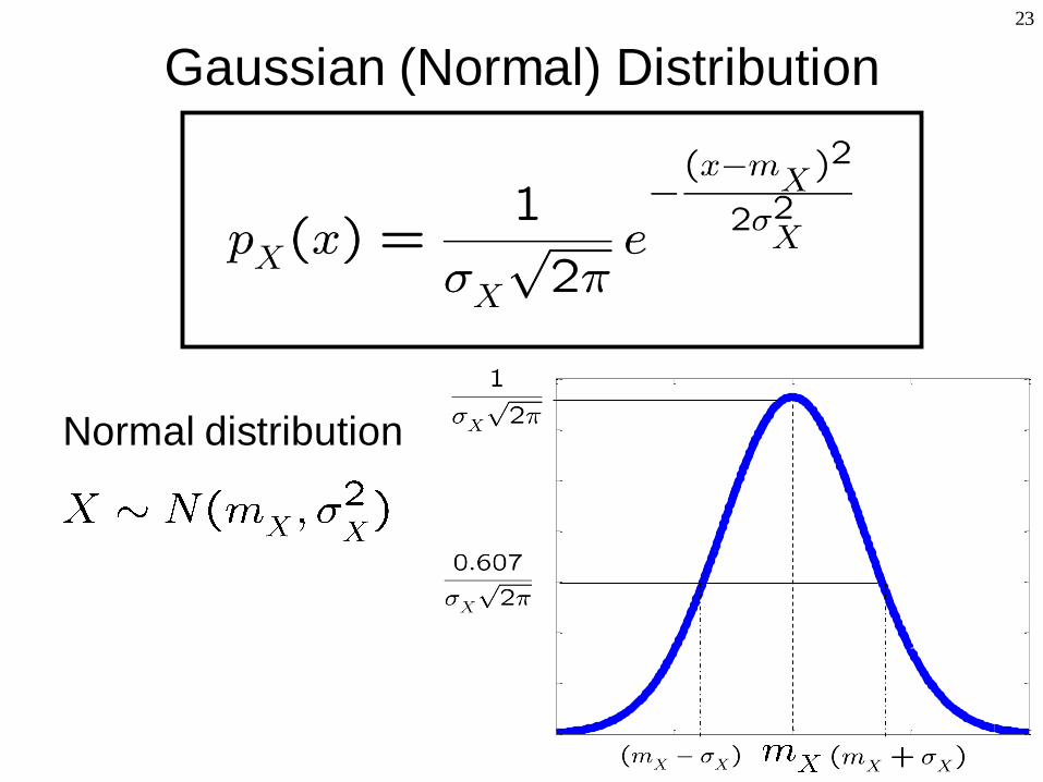
23

Gaussian (Normal) Distribution

Normal distribution

24

History of the Normal Distribution

From Wikipedia:

• The normal distribution was first introduced by de Moivre in an article in 1733 in the context of approximating certain binomial distributions for large n.

• His result was extended by Laplace in his book Analytical Theory of Probabilities (1812), and is now called the theorem of de Moivre-Laplace.

• Laplace used the normal distribution in the analysis of errors of experiments.

25

History of the Normal Distribution

From Wikipedia:

• The important method of least squares was introduced by Legendre in 1805.

• Gauss, who claimed to have used the method since 1794, justified it rigorously in 1809 by assuming a normal distribution of the errors.

• That the distribution is called the normal or Gaussian distribution is an instance of Stigler's law of eponymy: "No scientific discovery is named after its original discoverer."

26

Supplemental Material

(You are not responsible for this…)

• Laplace transform of normal PDF

• Proof of the central limit theorem

Laplace transform of normal PDF27

where, after “completing the squares”,

Laplace transform of normal PDF28

substituting,

= 1 (area under a PDF = 1)

Fourier transform:

Proof of the central limit theorem

Let X1, X2,... be independent random variables each with

mean mx and variance σx2 and define the sequence

29

where

notice that

Proof of the central limit theorem30

The moment generating function of Zn is

by the Taylor series expansion of ex

Proof of the central limit theorem31

notice that, as n →∞ the approximation is exact

Moreover, the PDF and moment generating function of a

normally distributed random variable are

and

Proof of the central limit theorem32

Therefore, since

Then, taking the inverse Fourier transform we obtain

and