matthias c. schabel nih public access edward v. r. dibella ... · a model-constrained monte carlo...

A Model-Constrained Monte Carlo Method for Blind Arterial InputFunction Estimation in Dynamic Contrast-Enhanced MRI: II) InVivo Results

Matthias C. Schabel, Edward V. R. DiBella, Randy L. Jensen, and Karen L. SalzmanUtah Center for Advanced Imaging Research, Department of Radiology, University of Utah HealthSciences Center, 729 Arapeen Drive, Salt Lake City UT 84108-1218Matthias C. Schabel: [email protected]

AbstractAccurate quantification of pharmacokinetic model parameters in tracer kinetic imagingexperiments requires correspondingly accurate determination of the arterial input function (AIF).Despite significant effort expended on methods of directly measuring patient-specific AIFs inmodalities as diverse as dynamic contrast-enhanced magnetic resonance imaging (DCE-MRI),dynamic positron emission tomography (PET), and perfusion computed tomography (CT),fundamental and technical difficulties have made consistent and reliable achievement of that goalelusive. Here, we validate a new algorithm for AIF determination, the Monte Carlo BlindEstimation (MCBE) method (which is described in detail and characterized by extensivesimulations in a companion paper), by comparing AIFs measured in DCE-MRI studies of eightbrain tumor patients with results of blind estimation. Blind AIFs calculated with the MCBEmethod using a pool of concentration-time curves from a region of normal brain tissue were foundto be quite similar to the measured AIFs, with statistically significant decreases in fit residualsobserved in six of eight patients. Biases between the blind and measured pharmacokineticparameters were the dominant source of error. Averaged over all eight patients, the mean biaseswere +7% in Ktrans, 0% in kep, −11% in vp, and +10% in ve. Corresponding uncertainties (medianabsolute deviation from best fit line) were 0.0043 min−1 in Ktrans, 0.0491 min−1 in kep, 0.29% invp, and 0.45% in ve. Use of a published population-averaged AIF resulted in larger mean biases inthree of the four parameters (−23% in Ktrans, −22% in kep, −63% in vp), with the bias in veunchanged, and led to larger uncertainties in all four parameters (0.0083 min−1 in Ktrans, 0.1038min−1 in kep, 0.31% in vp, and 0.95% in ve). When blind AIFs were calculated from a region oftumor tissue, statistically significant decreases in fit residuals were observed in all eight patientsdespite larger deviations of these blind AIFs from the measured AIFs. The observed decrease inroot-mean-square fit residuals between the normal brain and tumor tissue blind AIFs suggests thatthe local blood supply in tumors is measurably different from that in normal brain tissue and thatthe proposed method is able to discriminate between the two. We have shown the feasibility ofapplying the MCBE algorithm to DCE-MRI data acquired in brain, finding generally goodagreement with measured AIFs and decreased biases and uncertainties relative to use of apopulation-averaged AIF. These results demonstrate that the MCBE algorithm is a usefulalternative to direct AIF measurement in cases where acquisition of high-quality arterial inputfunction data is difficult or impossible.

KeywordsMagnetic resonance imaging; dynamic contrast-enhanced; DCE-MRI; arterial input function

NIH Public AccessAuthor ManuscriptPhys Med Biol. Author manuscript; available in PMC 2012 December 31.

Published in final edited form as:Phys Med Biol. 2010 August 21; 55(16): 4807–4823. doi:10.1088/0031-9155/55/16/012.

$waterm

ark-text$w

atermark-text

$waterm

ark-text

IntroductionDynamic contrast-enhanced magnetic resonance imaging (DCE-MRI), in conjunction withquantitative pharmacokinetic (PK) modeling, is becoming a standard method of acquiringnon-invasive imaging biomarkers for longitudinal studies in oncology and drug development(Leach et al. (2005)). DCE-MRI experiments typically involve rapid, repeated acquisition ofheavily T1-weighted images covering a tumor or other region of interest (ROI) before,during, and after bolus injection of a low molecular weight paramagnetic contrast agent(CA). Time courses of both blood and tissue contrast concentrations are determined from themeasured signal changes (Schabel & Parker (2008)), and the resulting curves subjected toregression analysis with one of a variety of pharmacokinetic (PK) models intended to extractphysiological parameters of the imaged tissues such as vascular permeability, blood flow,perfusion, interstitial volume, and microvessel density.

The Extended Tofts-Kety model (ETKM) is commonly used for pharmacokinetic analysis ofDCE-MRI data (Kershaw & Buckley (2006); Tofts et al. (1999)). In this model, the time-dependent contrast concentration in a tissue voxel, Ct(t), is described by:

(1)

where Cp(t) is the contrast concentration in the capillary blood plasma (also known as thearterial input function or AIF), Ktrans is the transfer rate constant, kep is the washout rateconstant, vp is the volume fraction of blood plasma, and the asterisk represents theconvolution operator.

Conventional approaches to the solution of Equation (1) involve regression of the modelfunction to the measured tissue concentration curves using a measured or population-averaged AIF. Regression provides estimates of the pharmacokinetic parameters Ktrans, kep,and vp, from which the extracellular extravascular volume, ve = Ktrans=kep, may becomputed. While this approach is straightforward, for reasons discussed in detail in acompanion paper (Schabel et al. (2010)) the need to measure both blood plasma and tissuecontrast concentrations simultaneously and accurately is problematic. Furthermore, evidencein the literature suggests that the AIF can be significantly delayed and/or dispersed bypassage through the vascular network between a large artery in which it is measured and thecapillary bed through which contrast molecules exchange with the tissues of interest(Calamante et al. (2006); Ko et al. (2007)). As a result, limited ability to accuratelydetermine the AIF is one of the major sources of uncertainty in DCE-MRI pharmacokineticmodeling (Port et al. (2001)).

Several methods have recently appeared in the literature that attempt to infer the AIF frommeasured tissue concentration curves, obviating the need to measure it directly (DiBella etal. (1999); Fluckiger et al. (2009); Riabkov & DiBella (2002, 2004); Walker-Samuel et al.(2007); Yang et al. (2004, 2009); Yankeelov et al. (2005, 2007)). In a companion paper wedescribe a new blind AIF estimation algorithm, called Monte Carlo Blind Estimation(MCBE), and characterize it with extensive computer simulations (Schabel et al. (2010)).This algorithm directly estimates the AIF from a set of measured tissue curves using aparameterized model function to constrain the functional form of the AIF, and requiresneither normal reference tissue curves nor clustering methods to accurately estimate theshape of the true AIF over a wide range of image acquisition parameters. Here we apply theMCBE algorithm to in vivo DCE-MRI data acquired in a group of eight patients withhistopathologically-confirmed brain tumors in which high-quality measured AIFs wereavailable and compare the performance of the MCBE method to the use of a measured AIF.

Schabel et al.

Phys Med Biol. Author manuscript; available in PMC 2012 December 31.

$waterm

ark-text$w

atermark-text

$waterm

ark-text

MethodsDCE-MRI Measurements

In vivo T1-weighted DCE-MRI data was acquired in eight brain cancer patients from whominformed consent was obtained under an Institutional Review Board (IRB)-approvedprotocol. All eight patients were scanned during standard stereotactic imaging prior tosurgery. Patient 7 had a clinical history of anteroseptal cardiac infarct, while patient 8 had aclinical history of myocardial infarction, coronary artery disease, diabetes, and transientischemic attack. Clinical histories of the remaining six patients showed no significantcardiovascular pathologies. After standard non-contrast imaging for pre-operative planningwas completed, the lesion of interest was identified and maps of pre-contrast longitudinalrelaxation time (T1,0) were measured using the variable flip angle (VFA) spoiled gradientecho (SPGR) method with flip angles of α = 3° and 20° (Schabel & Morrell (2009)). DCE-MRI measurements were then made using a fast three-dimensional SPGR sequence (fl3d) ona 1.5 T Siemens TIM Avanto scanner (four patients) or a 3 T Siemens TIM Trio and Verioscanners (four patients), with the same field of view used for the VFA T1,0 measurements.Pulse sequence parameters chosen to maximize sampling rate within constraints of adequatesignal-to-noise ratio (SNR) and coverage of the lesion of interest are given in Table 1 alongwith other relevant imaging and contrast injection data. Because DCE-MRI data wereacquired as add-on measurements to clinically-indicated stereotactic imaging prior to brainsurgery, imaging protocols varied slightly to accommodate different scanner hardware andSAR limits. Additional information including patient age, body mass, lesion location,clinical diagnosis, and location of the measured AIF is given in Table 2.

A standard (~0.1 mmol/kg) dose of low molecular weight gadolinium chelate contrast agent(Omniscan, GE Healthcare, or Multihance, Bracco Diagnostics) was injected into theantecubital vein through an 18–22 gauge IV followed by a saline flush using a powerinjector (Medrad Spectra Solaris), with volumes and injection rates as specified in Table 1.Contrast injection was timed to coincide with the end of acquisition of frame NB of thedynamic data. A twelve-channel transmit/receive head coil was used. Flip angle variationalong the slab encoding direction was estimated using a homogeneous phantom of knownT1,0, and, in three study patients, by assuming a constant T1,0 value of 240 ms forsubcutaneous fat. These experiments indicated that the impact of flip angle variation nearthe slab boundaries was small except for roughly the outer 10% of slices at each boundary.To minimize the potential for bias in conversion of signal to contrast concentration (Schabel& Parker (2008)), these slices were excluded from our analysis.

Pre-contrast signal intensity, S0, was determined by averaging the NB baseline images priorto injection and SNR was computed from the ratio of the baseline signal to its standarddeviation. Time curves of relative enhancement were generated from the time-dependentDCE-MRI signal, S(t), as Ξ(t) = (S(t)−S0)/S0. Tissue concentration-time curves, Ct(t), werethen computed by numerical solution of the full nonlinear concentration-dependence of theSPGR signal in the fast exchange limit (Schabel & Parker (2008)), with voxelwise tissueT1,0 values determined using the VFA method discussed above. Literature values for the T1

and relaxivities appropriate to the administered contrast agent at the imaging fieldstrength were used (Rohrer et al. (2005)). Concentration measurement uncertainties were

computed as described in Schabel & Parker (2008). The direct effect of on concentrationmeasurements is eliminated by the use of relative enhancement, and the very short TE values

used in imaging should result in minimal susceptibility-induced signal loss. A value of50 ms was assumed in calculations of contrast concentration uncertainty.

Schabel et al.


$waterm

ark-text$w

atermark-text

$waterm

ark-text

AIFs were obtained from the middle cerebral arteries in seven of the eight study patients. Inpatient 6 the middle cerebral arteries were not visible within the imaging field-of-view, sothe AIF was measured in the posterior superior sagittal sinus instead. A method similar tothat described in (Rijpkema et al. (2001)) was used to measure the AIF: curves of relativeenhancement within a manually-selected cuboidal ROI that reached their maximum valuewithin 30 seconds of initial bolus arrival and had a maximum enhancement corresponding toa concentration of at least 1 mM were identified. From among this set of curves, those withpeak Ξ values in the top 10% were selected and the median relative enhancement of theresulting curves was computed. This time curve of relative enhancement was then convertedto concentration in the same way as described for tissue curves (above) to obtain an estimateof the true AIF. A fixed pre-contrast longitudinal relaxation time for whole blood of T1,0 =1441 ms was assumed at 1.5T and 1932 ms at 3T (Stanisz et al. (2005)). We have attemptedto determine measured AIFs as accurately as possible, but, in the absence of a viable andindependent “gold standard” method for computing the true AIF in vivo, it must be assumedthat these measured AIFs are close to truth.

Blind AIF EstimationThe details of the MCBE algorithm are presented in a companion paper (Schabel et al.(2010)). For each patient, blind estimation was performed on two distinct pools of tissuecurves. The first pool of curves was selected from a cuboidal region of interest (ROI) placedin normal, non-pathologic tissue on the side of the brain contralateral to the known tumor,while the second pool was selected from an ROI covering the enhancing lesion. Images ofthese ROIs were assessed visually for early enhancement after contrast injection and theROIs adjusted as necessary to exclude any voxels showing enhancement patterns andmorphology obviously characteristic of arterial and/or venous voxels. Tissue curves havinga mean post-injection contrast concentration greater than or equal to 0.05 mM were thenselected from the curves within the specified ROI. This threshold value, roughly twice theaverage concentration measurement noise in these data sets, was empirically chosen toproduce a reasonable number of curves in the pool (M) with adequate signal-to-noise ratio(SNR). Provided there are sufficiently many curves for the algorithm to choose from (Mmuch greater than the number of curves per subset, D: M ≫ D), the specific method of curveselection appears to have relatively little impact on the performance of the blind estimationalgorithm. The initial bolus arrival time (as opposed to the known contrast injection time)was estimated from the median of the selected time curves by inspection.

When running the MCBE algorithm, we set the number of curves per subset to D = 12 andused 50 fixed iterations followed by 50 bootstrapping iterations (Q = 50 + 50*, Schabel et al.(2010)). Based on the simulations presented in the companion paper, these settings shouldbe sufficient to obtain good quality blind estimates, but we have not attempted to optimizethem for performance. Because measured tissue concentration curves are occasionallyaffected by artifacts arising from motion, poor estimates of T1,0, or other unmodeled effects,in our in vivo analysis we apply an auxiliary convergence check at each iteration. This checkconsists of comparing the median absolute deviation (MAD) of the fit residuals using thestarting AIF guess with the MAD using the blind AIF estimate, where:

(2)

This estimator is different from the χ2 estimator that is minimized by the nonlinearregression algorithm, so it serves as a means of identifying robust convergence; curve setsfor which χ2 decreases but MAD does not are rejected and a new curve set drawn. The finalblind AIF is normalized to the mean of the last ten measurements of the AIF. Variability in

Schabel et al.


$waterm

ark-text$w

atermark-text

$waterm

ark-text

blind AIF estimates was assessed by computing the 5th and 95th percentiles of the 50bootstrapping iterations, giving low and high bounds on blind AIFs at the 95% confidencelevel.

The performance of the MCBE algorithm was assessed in three ways: first by directlycomparing the blind and measured AIFs, second by comparing the root-mean-square (RMS)compartment model fit residuals of the tissue curves for the two AIFs, and third bygenerating joint probability density functions (JPDFs) of pharmacokinetic parameter valuesderived using the two AIFs. Model fit parameters were also computed using a populationAIF (Parker et al. (2006)) for comparison, with the arrival time of the population AIF set tothe arrival time of the blind AIF for consistency.

Statistical significance of changes in RMS fit residuals was computed, compensating for thepresence of additional free model parameters in the blind estimate, using the BayesInformation Criterion (BIC, Schwarz (1978)):

(3)

where the first term is the logarithm of the mean squared error, n is the number ofmeasurement time points, v is the number of voxels being compared, and k is the totalnumber of free parameters (3v for the measured AIF and 3v +10 for the blind AIF). Asmaller value of BIC indicates a statistically-significant improvement in quality of fit.

Biases and uncertainties in pharmacokinetic parameter values were determined using arobust linear regression algorithm (MATLAB’s robustfit function) to fit blind parameterestimates versus parameters computed using the measured AIF. Bias was computed from thelinear slope of the best fit line, while uncertainty was computed as the median absolutedeviation (a robust estimator of statistical dispersion) of the fit residuals (Huber (1990)). Fornormally-distributed data, standard deviation is related to MAD by σ ~ 1.48 MAD. Similarfits were performed on parameter estimates using the population AIF versus the measuredAIF.

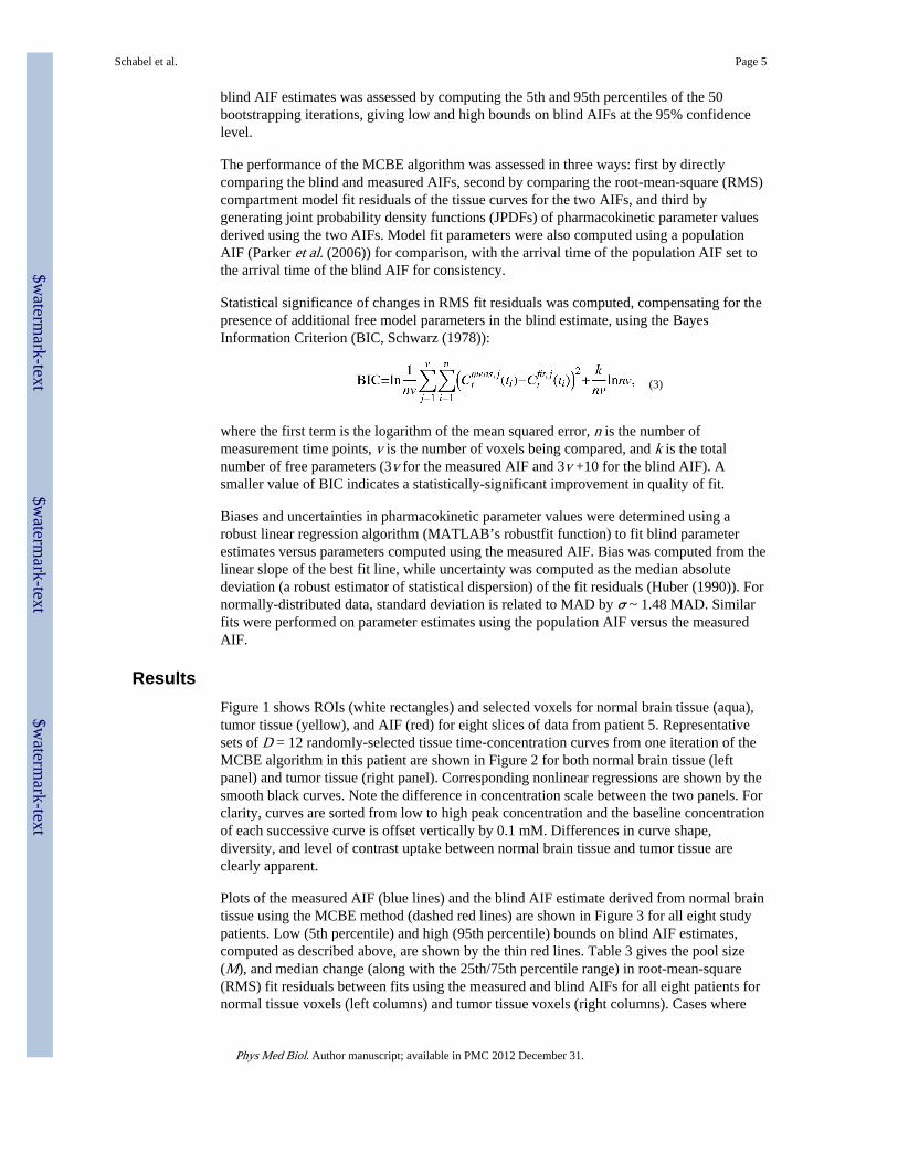
ResultsFigure 1 shows ROIs (white rectangles) and selected voxels for normal brain tissue (aqua),tumor tissue (yellow), and AIF (red) for eight slices of data from patient 5. Representativesets of D = 12 randomly-selected tissue time-concentration curves from one iteration of theMCBE algorithm in this patient are shown in Figure 2 for both normal brain tissue (leftpanel) and tumor tissue (right panel). Corresponding nonlinear regressions are shown by thesmooth black curves. Note the difference in concentration scale between the two panels. Forclarity, curves are sorted from low to high peak concentration and the baseline concentrationof each successive curve is offset vertically by 0.1 mM. Differences in curve shape,diversity, and level of contrast uptake between normal brain tissue and tumor tissue areclearly apparent.

Plots of the measured AIF (blue lines) and the blind AIF estimate derived from normal braintissue using the MCBE method (dashed red lines) are shown in Figure 3 for all eight studypatients. Low (5th percentile) and high (95th percentile) bounds on blind AIF estimates,computed as described above, are shown by the thin red lines. Table 3 gives the pool size(M), and median change (along with the 25th/75th percentile range) in root-mean-square(RMS) fit residuals between fits using the measured and blind AIFs for all eight patients fornormal tissue voxels (left columns) and tumor tissue voxels (right columns). Cases where

Schabel et al.


$waterm

ark-text$w

atermark-text

$waterm

ark-text

the change in RMS residuals was significant based on decreased value of BIC for all voxelswithin the curve pool, computed from Equation (3), are indicated by an asterisk.

Joint probability density functions comparing pharmacokinetic model parametersdetermined using the measured AIFs with those determined using the normal brain blindAIFs are shown in Figure 4. The JPDFs shown include all tissue voxels within the imagingFOV. Figures 5 and 6 present eight slices of data from Patients 4 and 5, respectively. Meanpost-contrast signal is shown in the top panel, with the lesion location indicated by yellowellipses. Pharmacokinetic parameter maps for Ktrans, ve, and vp computed using the blindAIF from normal brain are shown in the middle panel and those computed using themeasured AIF in the bottom panel.

Biases between the pharmacokinetic parameters determined from robust linear regression tothe JPDF data plotted in Figure 4, averaged over all eight patients, were +7% (range −8% to+32%) in Ktrans, 0% (range −9% to +16%) in kep, −11% (range −33% to +6%) in vp, and+10% (range −3% to +40%) in ve. Corresponding uncertainties were 0.0043 min−1 in Ktrans

(range 0.0008 min−1 to 0.0085 min−1), 0.0491 min−1 in kep (range 0.0187 min−1 to 0.0938min−1), 0.29% in vp (range 0.05% to 1.22%), and 0.45% in ve (range 0.12% to 0.80%). Useof the population-averaged AIF proposed by Parker et al. (2006) gave biases of : −23%(range −41% to −6%) in Ktrans, −22% (range −42% to +2%) in kep, −63% (range −87% to−39%) in vp, and +10% (range +3% to +22%) in ve, and uncertainties of : 0.0083 min−1 inKtrans (range 0.0032 min−1 to 0.0150 min−1), 0.1038 min−1 in kep (range 0.0515 min−1 to0.1854 min−1), 0.31% in vp (range 0.08% to 1.15%), and 0.95% in ve (range 0.30% to2.11%). Robust linear regression to JPDF data comparing the measured AIF to the blindtumor tissue AIF for tumor voxels alone, averaged over all eight patients, showed meanbiases of +7% (range −22% to +73%) in Ktrans, −13% (range −39% to +27%) in kep, −5%(range −36% to +41%) in vp, and +16% (range +3% to +27%) in ve. Correspondinguncertainties were 0.0053 min−1 in Ktrans (range 0.0014 min−1 to 0.0095 min−1), 0.0323min−1 in kep (range 0.0107 min−1 to 0.0719 min−1), 0.21% in vp (range 0.07% to 0.36%),and 0.59% in ve (range 0.08% to 1.07%).

The left panel of Figure 7 compares the measured AIF (blue) with the blind AIFs estimatedfrom normal brain tissue (dashed red line) and tumor tissue (dot-dashed black line) in patient4, in whom the greatest discrepancy between normal and tumor blind AIFs was observed.Maps of pharmacokinetic parameters for a single slice through the tumor are shown in theright panel, with Ktrans in the top row, kep in the second row, vp in the third row, and percentchange in RMS fit residuals between measured and blind AIFs in the fourth row. The mapscomputed using the measured AIF are plotted in the first column, with the normal tissueblind AIF in the second column, and with the tumor tissue blind AIF in the third column.Median parameter values derived from the normal tissue blind AIF, averaged over all tumorvoxels, were : Ktrans = 0.089 min−1, kep = 0.55 min−1, vp = 3.6%, and ve = 15.5%. Thesevalues showed a 15% increase in Ktrans relative to the measured AIF, an increase of 6% inkep, an increase of 1% in vp, and an increase of 8% in ve, with a median decrease in RMS fitresiduals of 2.1%. In contrast, use of the tumor AIF resulted in a 73% increase in Ktrans, anincrease of 27% in kep, an increase of 41% in vp, an increase of 22% in ve, and a decrease inRMS fit residuals of 8.2% in this patient.

DiscussionApplication of the Monte Carlo Blind Estimation algorithm to in vivo DCE-MRI dataacquired in eight brain tumor patients demonstrates that it is possible to accurately reproducemeasured arterial input functions using only concentration-time curves from normal braintissue. The blind AIFs shown in Figure 3 show good agreement with the measured AIFs, and

Schabel et al.


$waterm

ark-text$w

atermark-text

$waterm

ark-text

result in relatively small errors in pharmacokinetic parameter estimates that predominantlymanifest as linear biases (Figure 4). Statistically-significant decreases in the RMS model fitresiduals (Table 3) were observed in six of the eight patients using the blind AIF derivedfrom normal brain tissue, with residuals being comparable (within ±0.5%) to those from themeasured AIFs in the other two patients. These results suggest that the MCBE algorithm iscapable of extracting AIFs directly from tissue curves without inclusion of arterial voxels.The resulting model fits are at least as good as, and generally better than, those obtained bydirect measurement.

Our analysis of the MCBE method in vivo has two principal limitations. First, while weassume that the measured AIF is the reference “truth”, the reality is somewhat morecomplex due to the difficulty of making accurate measurements of arterial bloodconcentration in vivo (Cheng (2007)) as well as the further difficulty of assessing theuncertainty in those measurements. While we have attempted to minimize the effects of thenumerous difficulties associated with direct measurement of the arterial input function(discussed at length in the Introduction of the companion paper), the lack of an independent“gold-standard” measurement of the true AIF makes it difficult to determine the source andsignificance of discrepancies between measured and blind AIFs in this study.

Second, while the MCBE algorithm accurately reproduces the shape of measured AIFs inour study population, it cannot determine the global scale factor. This limitation arises fromthe fundamental invariance of Equation (1) to simultaneous rescaling of Cp(t), Ktrans, and vp(Schabel et al. (2010)). As a consequence, a single reference measurement of blood plasmacontrast concentration is needed to obtain quantitative pharmacokinetic parameter estimates.Here we have used the tails of the measured AIFs to provide the needed scale factor, whichreintroduces a dependence on blood pool measurements. In practice, however, this limitationis not severe. Because the needed measurement is obtained from the tail of the AIF, whenthe bolus is well-mixed in the blood pool, it is much less affected by saturation effects,arrival time, and limited temporal resolution than first-pass measurements. Furthermore, thisscale factor can be obtained, for example, by imaging a major artery or vein with a pulsesequence specifically tailored for quantitative blood pool concentration measurement (suchas one of the numerous quantitative T1 sequences) at the end of the data acquisition period.Nevertheless, a well-characterized, accurate, and thoroughly-validated MRI method forabsolute blood pool concentration measurement is needed for the MCBE algorithm to maketrue, quantitative estimates of the AIF and pharmacokinetic parameter values.

Another potential limitation of this study is the heterogeneity of acquisition parameters usedduring data collection, including contrast agent, scanner field strength, and imaging pulsesequence parameters. Since the processing and analysis methods used here compensated forknown differences in contrast agent relaxivities and imaging parameters, the primarysources of potential biases have been addressed. The absence of any obvious systematicdifferences in either AIF estimates or kinetic parameter values between the 1.5T and 3Tstudies, lends support to this contention.

In patients 3, 4, and 7 the measured and normal tissue blind AIFs show consistency betweenthe first-pass peak amplitude and width, recirculation peak, and tail height and slope. Patient6 shows very similar scale and shape, but a delay is clearly visible between the blind andmeasured AIFs; this delay presumably stems from the fact that the measured AIF wasdetermined from the venous sinuses in this patient rather than from the arterial blood, andprovides evidence that the MCBE algorithm is able to correctly determine the tissue bolusarrival time. Discrepancies are visible in the recirculation phase of the data from patients 1and 5, but otherwise the blind and measured AIFs show good agreement. In the former, theobserved discrepancy in the recirculation peak height lies outside the confidence bounds for

Schabel et al.


$waterm

ark-text$w

atermark-text

$waterm

ark-text

the blind AIF estimates, suggesting a systematic discrepancy, while the latter is mostlyconsistent with the upper variability bound of the blind estimates. The blind estimate of thefirst-pass peak height in patient 2 is approximately 20% greater than in the measured AIF,but the measured AIF still lies within the confidence bounds. Because most sources ofsystematic error in AIF measurement will tend to lead to underestimates in bolus peakheight (in particular saturation, finite sampling rate, and partial volume effects), this mayindicate the impact of one or more of these issues in the measured AIF in this patient.Finally, the width of the blind AIF in patient 8 is substantially different than measured,though the upslope and tail are in reasonable agreement and the upper blind confidencebound is consistent with the measured AIF. The visibly higher noise level in the measuredAIF in this patient indicates that it was of lower quality than those in the other sevenpatients. It is worth noting that the confidence bounds tend to be broadest in the first passpeak of the AIF, and narrowest in the tail region. Also notable is the presence of inter-patient variability in the tightness of the confidence bounds stemming from differences inthe signal-to-noise ratio (SNR), diversity, and size of the tissue curve pool used to generatethe blind AIF estimates.

The principal metric of concern for characterization of blind AIFs relative to measured AIFsis the accuracy with which pharmacokinetic model parameters can be estimated. Figure 4shows joint probability distribution functions for all eight study patients comparing values ofKtrans, kep, ve, and vp determined using the measured AIFs (x-axes) with values determinedusing the blind AIFs from normal brain tissue (y-axes). A white line drawn along thediagonals indicates the line of perfect agreement that would be achieved if there were exactcorrespondence between the two sets of parameter values. In all eight patients, there isstrong linear correlation between measured and blind parameter estimates of Ktrans, kep, andve and somewhat weaker correlation between vp values. Robust linear regression to JPDFdata shows that blind AIF estimates from normal tissue provide pharmacokinetic parameterestimates that generally have lower bias and uncertainty in the patient data than thoseobtained using a population-averaged AIF.

The presence of voxels with sufficient post-contrast enhancement to allow blind AIFestimation in both tumor and normal brain tissues is shown for patient 4 in Figure 1. Whilenearly all tumor voxels show enhancement reaching our chosen threshold value of post-contrast concentration, as indicated by the yellow voxels, fewer of those in the normal brain,shown in aqua, do so. This behavior is consistent with what is expected in the presence of anintact blood-brain barrier (BBB): enhancement of normal brain tissue stems primarily fromthe vascular contribution, with essentially no leakage of contrast into healthy brain tissue. Incontrast, brain tumors, particularly those with high tumor grade, demonstrate disruption ofthe BBB through elevated vascular permeability, an effect that is responsible for generallyhigher contrast concentration levels observed within tumors. Thus, the most strongly-enhancing voxels in intact brain tissue are generally those with a high vascular volume,while strongly-enhancing tumor voxels may arise from regions with either high vascularvolume or high vascular permeability, with disruption of the BBB enhancingtransendothelial contrast transport.

Contrast concentration-time curves shown in Figure 2 for normal brain tissue (left panel)and tumor tissue (right panel) clearly demonstrate the differences between the characteristicuptake in these two tissues. Peak and mean concentrations in normal brain tissue are bothsignificantly lower than those in tumor, curve shape is generally more similar to a purelyvascular signal (with an early rise to peak followed by a decreasing tail), and diversity incurve shape is generally lower. Nevertheless, in both normal and tumor tissues, the MCBEalgorithm converges robustly, consistent with the simulation results presented in thecompanion paper. Blind AIF estimates derived from tumor tissues show statistically-

Schabel et al.


$waterm

ark-text$w

atermark-text

$waterm

ark-text

significant decreases in fit residuals for tumor voxels in all eight patients, and somecharacteristic differences are seen when comparing to the measured AIFs. In particular, in anumber of blind tumor AIFs the recirculation and washout phases appear to be suppressedrelative to those in normal tissue blind AIFs, and there is a perceptible lag in the leadingedge of contrast arrival in the blood pool.

Our observation that blind AIFs estimated directly from tumor tissue curves deviate fromthose estimated from normal tissues in the same patients is consistent with results insarcomas (Fluckiger et al. (2009)), where it was found that blind AIF estimates from tumortissue ROIs manifested delay and dispersion relative to the AIF measured in arterial blood.The idea of a local AIF is also supported by observation of delay and dispersion of the AIFin dynamic susceptibility contrast (DSC) studies in the brain (Calamante et al. (2006); Ko etal. (2007)). Despite this, the inability to directly validate predicted discrepancies between theAIF in normal brain tissue and the AIF in tumor tissue remains a limitation of the workdescribed here. Some support can be inferred from changes in RMS fit residuals. Observedchanges in fit residuals using the normal brain blind AIF are smaller, and are relativelyuniform and consistent throughout the brain. In contrast, the tumor blind AIFs generallyshow large decreases in RMS residuals in the tumor itself, but minimal changes or increasesin unaffected brain tissues.

The discussion here has focused on the ETKM, but the methods described are easilyextended to subsume different types of pharmacokinetic models such as those that accountfor spatial variation in bolus arrival time (Orton et al. (2007)), finite capillary filling times(Koh et al. (2006); St. Lawrence & Lee (1998)), or deviation of water exchange from thefast exchange limit (Li et al. (2005)). Indeed, while our analysis emphasizes tissueconcentration curves derived from DCE-MRI measurements, data from any quantitativeimaging modality (such as CT, PET, and SPECT) could be used instead. The MCBE methodappears to be a practical and effective algorithm for blind AIF estimation that generalizesearlier algorithms relying on clustering of tissue curves.

AcknowledgmentsM. C. S. and E. V. R. D. would like to thank the Ben and Iris Margolis Foundation and the Benning Foundation fortheir support of this work. M. C. S. also gratefully acknowledges the National Institute for Biomedical Imaging andBioengineering for its support of this work through the K25 Career Development Award #K25EB005077.

ReferencesCalamante, Fernando; Willats, Lisa; Gadian, David G.; Connelly, Alan. Bolus delay and dispersion in

perfusion MRI: implications for tissue predictor models in stroke. Magn Reson Med. 2006; 55(5):1180–5. [PubMed: 16598717]

Cheng, Hai-Ling Margaret. T1 measurement of flowing blood and arterial input function determinationfor quantitative 3D T1-weighted DCE-MRI. J Magn Reson Imaging. 2007; 25(5):1073–8. [PubMed:17410576]

DiBella EV, Clackdoyle R, Gullberg GT. Blind estimation of compartmental model parameters. PhysMed Biol. 1999; 44(3):765–80. [PubMed: 10211809]

Fluckiger J, Schabel MC, DiBella EVR. Model-based blind estimation of kinetic parameters indynamic contrast enhanced (DCE)-MRI. Magn Reson Med. 2009; 62(6):1477–1486. [PubMed:19859949]

Huber, PJ. Robust Statistics. John Wiley and Sons; New York: 1981.

Kershaw, Lucy E.; Buckley, David L. Precision in measurements of perfusion and microvascularpermeability with T1-weighted dynamic contrast-enhanced MRI. Magn Reson Med. 2006; 56(5):986–92. [PubMed: 16986107]

Schabel et al.


$waterm

ark-text$w

atermark-text

$waterm

ark-text

Ko, Linda; Salluzzi, Marina; Frayne, Richard; Smith, Michael. Reexamining the quantification ofperfusion MRI data in the presence of bolus dispersion. J Magn Reson Imaging. 2007; 25(3):639–43. [PubMed: 17326085]

Koh TS, Cheong LH, Tan CK, Lim CC. A distributed parameter model of cerebral blood-tissueexchange with account of capillary transit time distribution. Neuroimage. 2006; 30(2):426–35.[PubMed: 16246589]

Leach MO, Brindle KM, Evelhoch JL, Griffiths JR, Horsman MR, Jackson A, Jayson GC, Judson IR,Knopp MV, Maxwell RJ, McIntyre D, Padhani AR, Price P, Rathbone R, Rustin GJ, Tofts PS,Tozer GM, Vennart W, Waterton JC, Williams SR, Workman P. The assessment of antiangiogenicand antivascular therapies in early-stage clinical trials using magnetic resonance imaging: issues andrecommendations. Br J Cancer. 2005; 92(9):1599–610. [PubMed: 15870830]

Li, Xin; Rooney, William D.; Springer, Charles S. A unified magnetic resonance imagingpharmacokinetic theory: intravascular and extracellular contrast reagents. Magn Reson Med. 2005;54(6):1351–9. [PubMed: 16247739]

Orton MR, Collins DJ, Walker-Samuel S, d’Arcy JA, Hawkes DJ, Atkinson D, Leach MO. Bayesianestimation of pharmacokinetic parameters for DCE-MRI with a robust treatment of enhancementonset time. Phys Med Biol. 2007; 52(9):2393–408. [PubMed: 17440242]

Parker, Geoff JM.; Roberts, Caleb; Macdonald, Andrew; Buonaccorsi, Giovanni A.; Cheung, Sue;Buckley, David L.; Jackson, Alan; Watson, Yvonne; Davies, Karen; Jayson, Gordon C.Experimentally-derived functional form for a population-averaged high-temporal-resolutionarterial input function for dynamic contrast-enhanced MRI. Magn Reson Med. 2006; 56(5):993–1000. [PubMed: 17036301]

Port RE, Knopp MV, Brix G. Dynamic contrast-enhanced MRI using Gd-DTPA: Interindividualvariability of the arterial input function and consequences for the assessment of kinetics in tumors.Magn Reson Med. 2001; 45:1030–1038. [PubMed: 11378881]

Riabkov, Dmitri Y.; DiBella, Edward VR. Estimation of kinetic parameters without input functions:analysis of three methods for multichannel blind identification. IEEE Trans on Biomed Eng. 2002;49(11):1318–27.

Riabkov, Dmitri Y.; DiBella, Edward VR. Blind identification of the kinetic parameters in three-compartment models. Phys Med Biol. 2004; 49(5):639–64. [PubMed: 15070194]

Rijpkema M, Kaanders JH, Joosten FB, van der Kogel AJ, Heerschap A. Method for quantitativemapping of dynamic MRI contrast agent uptake in human tumors. J Magn Reson Imaging. 2001;14(4):457–63. [PubMed: 11599071]

Rohrer M, Bauer H, Mintorovitch J, Requardt M, Weinmann HJ. Comparison of magnetic propertiesof MRI contrast media solutions at different magnetic field strengths. Invest Radiol. 2005; 40(11):715–24. [PubMed: 16230904]

Schabel, Matthias C.; Fluckiger, Jacob U.; DiBella, Edward VR. A Model-Constrained Monte CarloMethod for Blind Arterial Input Function Estimation in Dynamic Contrast-Enhanced MRI : I)Simulations. Phys Med Biol. 2010; XX(X):XX–XX.

Schabel, Matthias C.; Morrell, Glen R. Uncertainty in T(1) mapping using the variable flip anglemethod with two flip angles. Phys Med Biol. 2009; 54(1):N1–8. [PubMed: 19060359]

Schabel, Matthias C.; Parker, Dennis L. Uncertainty and bias in contrast concentration measurementsusing spoiled gradient echo pulse sequences. Phys Med Biol. 2008; 53(9):2345–73. [PubMed:18421121]

Schwarz G. Estimating the dimension of a model. The Annals of Statistics. 1978; 6(2):461–464.

StLawrence KS, Lee TY. An adiabatic approximation to the tissue homogeneity model for waterexchange in the brain : I. theoretical derivation. J Cereb Blood Flow Metab. 1998; 18:1365–1377.[PubMed: 9850149]

Stanisz, Greg J.; Odrobina, Ewa E.; Pun, Joseph; Escaravage, Michael; Graham, Simon J.; Bronskill,Michael J.; Henkelman, R Mark. T1, T2 relaxation and magnetization transfer in tissue at 3T.Magn Reson Med. 2005; 54(3):507–512. [PubMed: 16086319]

Tofts PS, Brix G, Buckley David L, Evelhoch JL, Henderson E, Knopp MV, Larsson HB, Lee TY,Mayr NA, Parker GJ, Port RE, Taylor J, Weisskoff RM. Estimating kinetic parameters from

Schabel et al.


$waterm

ark-text$w

atermark-text

$waterm

ark-text

dynamic contrast-enhanced T(1)-weighted MRI of a diffusable tracer: standardized quantities andsymbols. J Magn Reson Imaging. 1999; 10(3):223–32. [PubMed: 10508281]

Walker-Samuel S, Parker CC, Leach MO, Collins DJ. Reproducibility of reference tissuequantification of dynamic contrast-enhanced data: comparison with a fixed vascular inputfunction. Phys Med Biol. 2007; 52(1):75–89. [PubMed: 17183129]

Yang, Cheng; Karczmar, Gregory S.; Medved, Milica; Stadler, Walter M. Estimating the arterial inputfunction using two reference tissues in dynamic contrast-enhanced MRI studies: fundamentalconcepts and simulations. Magn Reson Med. 2004; 52(5):1110–7. [PubMed: 15508148]

Yang, Cheng; Karczmar, Gregory S.; Medved, Milica; Oto, Aytekin; Zamora, Marta; Stadler, WalterM. Reproducibility assessment of a multiple reference tissue method for quantitative dynamiccontrast enhanced-MRI analysis. Magn Reson Med. 2009; 61(4):851–9. [PubMed: 19185002]

Yankeelov, Thomas E.; Luci, Jeffrey J.; Lepage, Martin Li; Rui, Debusk; Laura, Lin; Charles, P.;Price, Ronald R.; Gore, John C. Quantitative pharmacokinetic analysis of DCE-MRI data withoutan arterial input function: a reference region model. Magn Reson Imaging. 2005; 23(4):519–29.[PubMed: 15919597]

Yankeelov, Thomas E.; Cron, Greg O.; Addison, Christina L.; Wallace, Julia C.; Wilkins, Ruth C.;Pappas, Bruce A.; Santyr, Giles E.; Gore, John C. Comparison of a reference region model withdirect measurement of an AIF in the analysis of DCE-MRI data. Magn Reson Med. 2007; 57(2):353–61. [PubMed: 17260371]

Schabel et al.


$waterm

ark-text$w

atermark-text

$waterm

ark-text

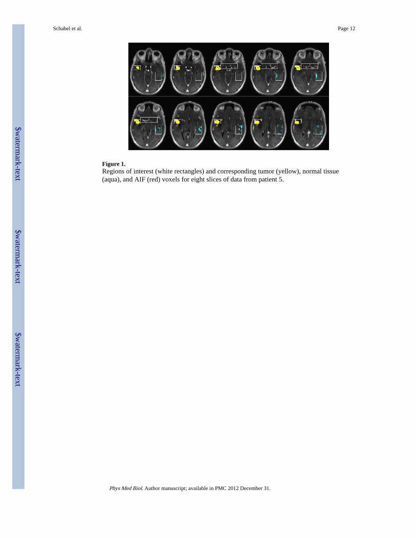
Figure 1.Regions of interest (white rectangles) and corresponding tumor (yellow), normal tissue(aqua), and AIF (red) voxels for eight slices of data from patient 5.

Schabel et al.


$waterm

ark-text$w

atermark-text

$waterm

ark-text

Figure 2.Twelve tissue curves (gray lines) and corresponding nonlinear regressions (black lines) for asingle MCBE subset (D = 12) of normal brain tissue (left panel) and tumor tissue (rightpanel) from patient 5 are shown. Successive curves are offset vertically by 0.1 mM forvisual clarity.

Schabel et al.


$waterm

ark-text$w

atermark-text

$waterm

ark-text

Figure 3.Plots comparing the measured AIF (solid blue lines) and the blind AIF derived from normalbrain tissue (dashed red lines) for all eight study patients. 5th and 95th percentile confidencebounds on the blind AIF estimates are shown by the thin red lines.

Schabel et al.


$waterm

ark-text$w

atermark-text

$waterm

ark-text

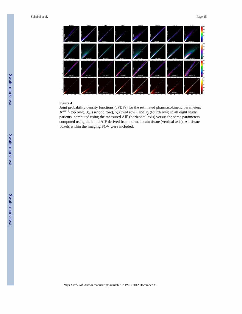
Figure 4.Joint probability density functions (JPDFs) for the estimated pharmacokinetic parametersKtrans (top row), kep (second row), ve (third row), and vp (fourth row) in all eight studypatients, computed using the measured AIF (horizontal axis) versus the same parameterscomputed using the blind AIF derived from normal brain tissue (vertical axis). All tissuevoxels within the imaging FOV were included.

Schabel et al.


$waterm

ark-text$w

atermark-text

$waterm

ark-text

Figure 5.Comparison of pharmacokinetic model fitting in patient 4, using the measured AIF and theblind AIF derived from normal brain tissue. Eight slices are shown, with mean post-contrastsignal in the upper panel. A yellow ellipse is used to indicate the lesion location on the meansignal images. The middle panel shows Ktrans (min−1), ve, and vp computed using the blindAIF in the first, second, and third rows, respectively. The lower panel shows the sameparameters computed using the measured AIF.

Schabel et al.


$waterm

ark-text$w

atermark-text

$waterm

ark-text

Figure 6.Comparison of pharmacokinetic model fitting in patient 5, using the measured AIF and theblind AIF derived from normal brain tissue, plotted as in Figure 5. Note that the upper rangeof Ktrans extends to 1 min−1 in this figure.

Schabel et al.


$waterm

ark-text$w

atermark-text

$waterm

ark-text

Figure 7.Comparison of the measured AIF (blue), blind AIF derived from normal tissue (dashed redline), and blind AIF derived from tumor tissue (dot-dashed black line) for patient 4 (leftpanel). Corresponding maps of the pharmacokinetic parameters for a single slice through thetumor, along with percent change in root-mean-square fit residuals for the normal blind andtumor blind AIFs relative to fitting with the measured AIF (ΔRMS), are shown in the rightpanel.

Schabel et al.


$waterm

ark-text$w

atermark-text

$waterm

ark-text

$waterm

ark-text$w

atermark-text

$waterm

ark-text

Schabel et al.

Tabl

e 1

MR

I pa

ram

eter

s fo

r th

e D

CE

-MR

I sc

ans

perf

orm

ed in

8 s

tudy

pat

ient

s. R

epet

ition

tim

e (T

R)

and

echo

tim

e (T

E)

are

give

n in

mill

isec

onds

, flip

ang

le (α)

in d

egre

es, r

esol

utio

n in

mm

, len

gth

of d

ynam

ic s

can

(tm

ax)

in m

inut

es, s

ampl

ing

inte

rval

(Δ

t) in

sec

onds

, and

tota

l adm

inis

tere

d co

ntra

st d

ose

in m

mol

/kg

of

body

mas

s. T

otal

num

ber

of s

cans

(N

mea

s) is

giv

en a

long

with

num

ber

of s

cans

pri

or to

con

tras

t inj

ectio

n (N

B).

Con

tras

t inj

ectio

n in

form

atio

n is

prov

ided

as

VC

/RC

CA

+ V

S/R

S, w

here

VC

rep

rese

nts

the

volu

me

of c

ontr

ast i

njec

ted

(ml)

, RC

the

rate

of

cont

rast

inje

ctio

n (m

l/s),

CA

the

cont

rast

age

ntus

ed (

eith

er O

mni

scan

, OS,

or

Mul

tihan

ce, M

H),

VS

the

volu

me

of s

alin

e fl

ush

inje

cted

(m

l), a

nd R

S th

e ra

te o

f sa

line

inje

ctio

n (m

l/s).

Pat

ient

Fie

ldT

RT

Eα

Mat

rix

Res

olut

ion

t max

Δt

Nm

eas

NB

Con

tras

t in

ject

ion

Dos

e

13T

2.80

1.02

17°

128

× 8

8 ×

24

2.0

× 2

.0 ×

3.0

7.65

3.86

120

1020

/4 M

H +

20/

20.

103

23T

2.82

1.04

17°

128

× 8

8 ×

32

2.0

× 2

.0 ×

2.0

7.6

4.60

100

1016

/2 M

H +

20/

20.

086

33T

2.73

0.88

19°

128

× 6

4 ×

32

2.5

× 2

.5 ×

2.5

6.40

3.23

120

1010

/2.5

MH

+ 2

0/4

0.07

9

41.

5T3.

081.

1820

°12

8 ×

104

× 3

21.

7 ×

1.7

× 2

.08.

365.

9785

2020

/4 O

S +

20/

20.

085

51.

5T3.

081.

1920

°12

8 ×

96

× 3

21.

8 ×

1.8

× 1

.87.

43.

7412

020

12/4

MH

+ 2

0/2

0.09

8

63T

2.91

1.08

18°

128

× 1

04 ×

24

1.6

× 1

.6 ×

2.0

7.4

3.00

150

1019

/4 M

H +

20/

20.

089

71.

5T2.

921.

0925

°12

8 ×

104

× 3

61.

5 ×

1.5

× 1

.58.

45.

1012

010

10/4

MH

+ 2

0/2

0.09

2

81.

5T3.

451.

3815

°25

6 ×

224

× 1

60.

9 ×

0.9

× 5

.08.

114.

2311

510

20/4

OS

+ 2

0/2

0.09

4


$waterm

ark-text$w

atermark-text

$waterm

ark-text

Schabel et al.

Tabl

e 2

Patie

nt, l

esio

n, a

nd A

IF m

easu

rem

ent i

nfor

mat

ion

for

the

eigh

t stu

dy p

artic

ipan

ts.

Pat

ient

Age

(yr

)W

eigh

t (k

g)L

esio

n lo

cati

onD

iagn

osis

Mea

sure

d A

IF

164

97.5

R te

mpo

ral l

obe

glio

blas

tom

a m

ultif

orm

em

iddl

e ce

rebr

al a

rter

y

243

92.5

L te

mpo

ral l

obe

glio

blas

tom

a m

ultif

orm

em

iddl

e ce

rebr

al a

rter

y

349

63.5

R te

mpo

ral l

obe

glio

blas

tom

a m

ultif

orm

em

iddl

e ce

rebr

al a

rter

y

451

117.

9R

par

ieta

l lob

egl

iobl

asto

ma

mul

tifor

me

mid

dle

cere

bral

art

ery

522

60.9

R te

mpo

ral l

obe

pleo

mor

phic

xan

thoa

stro

cyto

ma

mid

dle

cere

bral

art

ery

620

106.

6L

tem

pora

l lob

egl

iobl

asto

ma

mul

tifor

me

post

erio

r su

peri

or s

agitt

al s

inus

770

54.4

R te

mpo

ral l

obe

men

ingi

oma

mid

dle

cere

bral

art

ery

868

106

L te

mpo

ral l

obe

glio

blas

tom

a m

ultif

orm

em

iddl

e ce

rebr

al a

rter

y


$waterm

ark-text$w

atermark-text

$waterm

ark-text

Schabel et al.

Tabl

e 3

Pool

siz

e, M

, and

med

ian

and

25th

/75t

h pe

rcen

tile

chan

ges

in R

MS

fit r

esid

uals

bet

wee

n m

easu

red

and

blin

d A

IFs

for

voxe

ls w

ithin

the

norm

al b

rain

or

tum

or R

OI

whe

re b

oth

Ktr

ans

and

k ep

wer

e si

gnif

ican

t at t

he 9

5% le

vel.

Ast

eris

ks in

dica

te c

ases

whe

re f

it qu

ality

(qu

antif

ied

by th

e B

ayes

Inf

orm

atio

nC

rite

rion

) w

as s

igni

fica

ntly

bet

ter

for

the

blin

d A

IF e

stim

ate

than

for

the

mea

sure

d A

IF.

Pat

ient

norm

al b

rain

RO

Itu

mor

RO

I

MΔ

RM

S25

%/7

5%M

ΔR

MS

rang

e

125

3−

1.5%

*(−

5.0%

/+0.

5%)

321

−9.

0%*

(−21

.6%

/−1.

9%)

248

7−

0.4%

(−0.

4%/+

2.6%

)11

17−

2.9%

*(−

6.7%

/+0.

1%)

332

4−

3.2%

*(−

8.4%

/−0.

8%)

890

−20

.0%

*(−

33.3

%/−

8.8%

)

434

1−

0.3%

*(−

1.1%

/+0.

1%)

919

−8.

2%*

(−15

.3%

/−2.

4%)

521

8−

1.0%

*(−

3.8%

/+0.

0%)

850

−3.

4%*

(−7.

7%/−

0.6%

)

613

3−

1.7%

*(−

5.6%

/−0.

3%)

974

−4.

4%*

(−10

.6%

/−1.

6%)

710

38−

3.4%

*(−

7.1%

/−1.

0%)

2333

−12

.3%

*(−

19.4

%/−

5.4%

)

884

2+

0.3%

(−0.

5%/+

1.2%

)51

67−

0.4%

*(−

2.1%

/+1.

0%)


matthias c. schabel nih public access edward v. r. dibella ... · a model-constrained monte carlo...

Documents