matlab program related optics project

1

CHAPTER 1

TV HOLOGRAPHY

1.1. Introduction and Basic Theory

TV Holography (TVH) also known as Electronic/Digital Speckle Pattern Interferometry

(ESPI/DSPI) or Phase Shifting Speckle Interferometry (PSSI) is a reliable non-contact

optical technique for quantitative measuring displacement components of a deformation

vector of a diffusely scatter object under static or dynamic load [1-2]. The method is

based on speckle correlation using the direct electronic/digital subtraction of the

intensities in the initial and deformed state of the object. The ability to measure three

dimensional surface profiles by generating the contours of constant depth of an object is

yet another major achievement of TV holography. The range of the object that can be

evaluated by TV Holography is the order of few hundreds microns to few meter.

This technique is normally used in two modes: addition or subtraction speckle correlation

mode and time average mode. Addition or subtraction mode is used in deformation

analysis, means it is used to measure the displacement components and shape of the

object. Time average mode is applied vibration analysis. In this project subtraction

speckle correlation mode of operation is used.

In this mode the diffuse surface in its initial state, one frame of the interference speckle

fields (object and reference beams combined at the CCD plane) is recorded on video

store. Now the object is deformed and the current frame speckle field is subtracted

electronically pixel by pixel from the stored frame. The correlation spackle fringes are

displayed on the monitor in real time.

Here speckle pattern is a granular structure, which is formed in space when a coherent

wave from a laser is reflected from or transmitted through an optically rough surface. The

intensity distribution in the image of a diffused surface, when it is illuminated by a

2

coherent wave also exhibits granular structure [1-2]. This speckle pattern is called a

subjective speckle pattern.

Let 1I and I2 be the irradiance distribution incident on a camera face plate before and after

the object is deformed. Then the intensity before and after the displacement can be

expressed as [1-2]

1 2 cos( )O R O RI I I I I (1.1)

2 2 cos( )O R O RI I I I I (1.2)

where OI and RI are irradiance of object wave and reference wave respectively. is the

phase of the random speckle and is the phase change due to object deformation.

Video signal are assumed to be proportional to the irradiances. So the subtracted video

signal SV will be

2 1 2 cos( ) cos( )S O RV I I I I (1.3)

Therefore the brightness B on

2 1 sin( 2)sin( 2)O RB I I C I I (1.4)

where C is proportionality constant. sin( / 2) represents the speckle noise which

varies randomly between object images, because it is sin function of . Equation (1.4)

describes the modulation of high frequency noise by a low frequency interference pattern

related to phase change .

3

The condition for minimum B is that,

sin( / 2) 0 (1.5)

when ever 2n n = 0, 1, 2…….

This condition corresponds to dark fringes and denotes all of those regions where the

speckle patterns are correlated. The condition for maximum B is that,

sin( / 2) 1 (1.6)

when ever, (2 1)n n=0, 1, 2……..

This condition corresponds to bright fringes and denotes all of those regions where the

speckle patterns are uncorrelated. As a result, the speckle correlation fringes that

represent the contour of constant phase are seen in monitor. From monitor we have seen

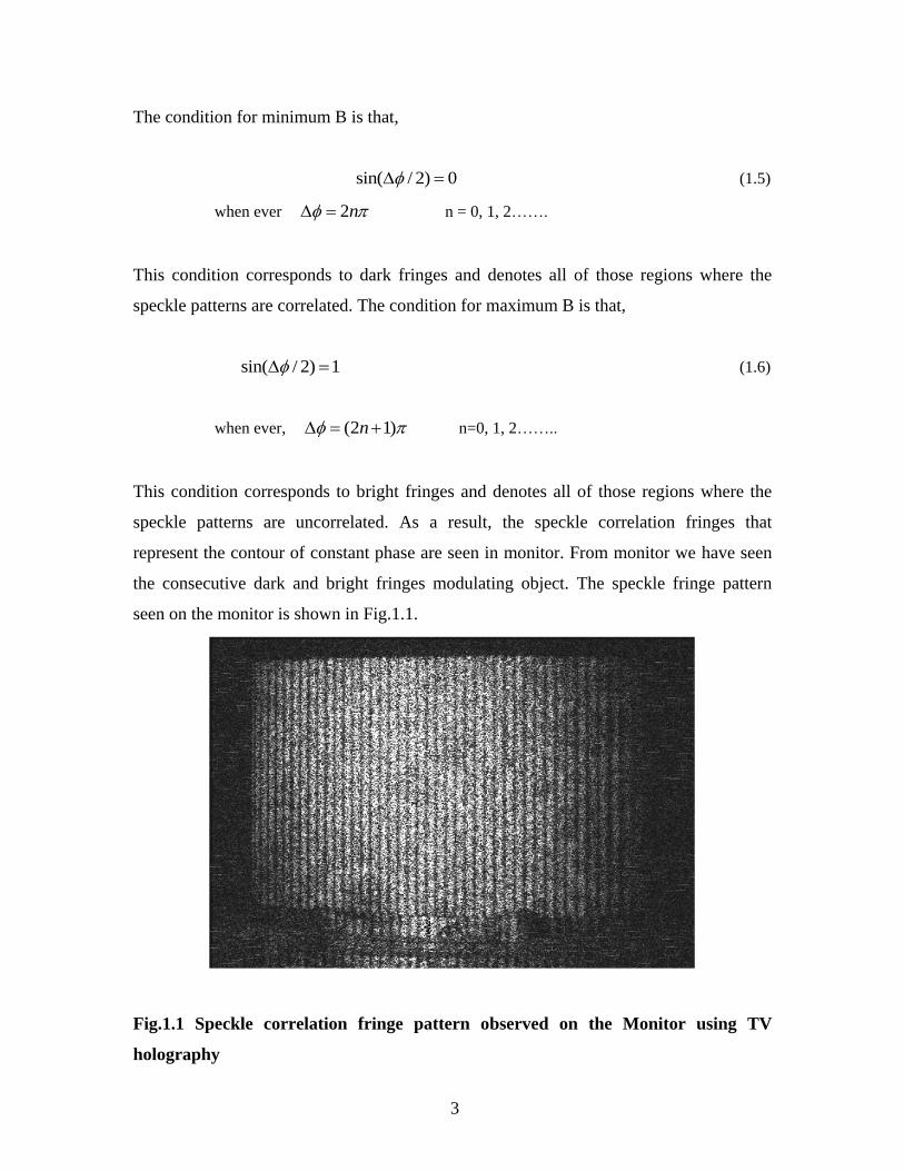
the consecutive dark and bright fringes modulating object. The speckle fringe pattern

seen on the monitor is shown in Fig.1.1.

Fig.1.1 Speckle correlation fringe pattern observed on the Monitor using TV

holography

4

The phase change is directly related to deformation vector ( , , )L u v w

; , ,u v w are the

displacement component along , ,x y z directions respectively. So we have to measure the

phase change . We can arrange the optical head of the system in several different ways

for measuring the shape and as well as the deformation. The different methods for shape

measurement of a 3-D object are described here.

1.2 Shape Measurement

TV holography is suitable for measurement of the shape of 3-D objects. It generates the

contours of constant depth of a curved object. The existing methods used for shape are

described below [1-7]

(a) Multiple Wavelength Method

In this method, two or multiple wavelength is used for shape measurement. The multiple

wavelength yields the effective wavelength and it can be directly related to the shape of

the object [3].

Consider two wavelengths 1 and 2 is used either sequentially or simultaneously for

recording. The difference between the two phases 1 2, corresponds to the wavelengths

1 and 2 respectively can be related to the surface depth of the object, „Z‟ as [3]

1 2 12

4Z

(1.7)

where, 1 2

1 2

; is the effective wavelength.

The depth contour interval depends on the effective wavelength .

5

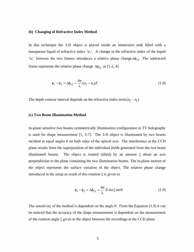
(b) Changing of Refractive Index Method

In this technique the 3-D object is placed inside an immersion tank filled with a

transparent liquid of refractive index „n1‟. A change in the refractive index of the liquid

„n2‟ between the two frames introduces a relative phase change 12 . The subtracted

frame represents the relative phase change 12 as [1-2, 4]

1 2 12 2 1

4( )n n Z

(1.8)

The depth contour interval depends on the refractive index term 2 1( )n n .

(c) Two Beam Illumination Method

In-plane sensitive two beams symmetrically illumination configuration in TV holography

is used for shape measurement [1, 5-7]. The 3-D object is illuminated by two beams

incident at equal angles θ on both sides of the optical axis. The interference at the CCD

plane results from the superposition of the individual fields generated from the two beam

illuminated beams. The object is rotated (tilted) by an amount ξ about an axis

perpendicular to the plane containing the two illumination beams. The in-plane motion of

the object represents the surface variation of the object. The relative phase change

introduced in the setup as result of this rotation ξ is given as

1 2 12

4sin sinZ

(1.9)

The sensitivity of the method is dependent on the angle θ. From the Equation (1.9) it can

be noticed that the accuracy of the shape measurement is dependent on the measurement

of the rotation angle ξ given to the object between the recordings at the CCD plane.

6

In this project work, we propose to develop a three beam illumination configuration in

TV holography for the measurement of object rotation angle ξ that is required for precise

evaluation of the shape of the 3-D object. The in-plane sensitive configuration is

combined with an out-of-plane sensitive arrangement for measurements. The three beam

illumination TV holographic setup is discussed in Chapter 2.

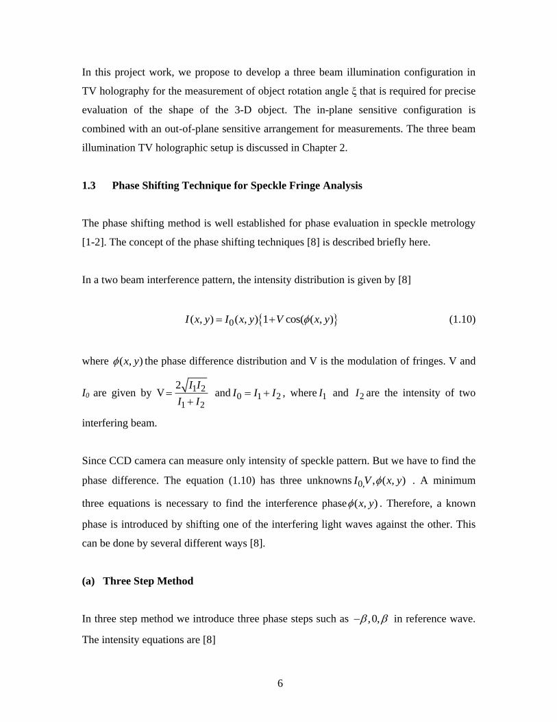
1.3 Phase Shifting Technique for Speckle Fringe Analysis

The phase shifting method is well established for phase evaluation in speckle metrology

[1-2]. The concept of the phase shifting techniques [8] is described briefly here.

In a two beam interference pattern, the intensity distribution is given by [8]

0( , ) ( , ) 1 cos( ( , )I x y I x y V x y (1.10)

where ( , )x y the phase difference distribution and V is the modulation of fringes. V and

I0 are given by V 1 2

1 2

2 I I

I I

and 0 1 2I I I , where 1I and 2I are the intensity of two

interfering beam.

Since CCD camera can measure only intensity of speckle pattern. But we have to find the

phase difference. The equation (1.10) has three unknowns 0, , ( , )I V x y . A minimum

three equations is necessary to find the interference phase ( , )x y . Therefore, a known

phase is introduced by shifting one of the interfering light waves against the other. This

can be done by several different ways [8].

(a) Three Step Method

In three step method we introduce three phase steps such as ,0, in reference wave.

The intensity equations are [8]

7

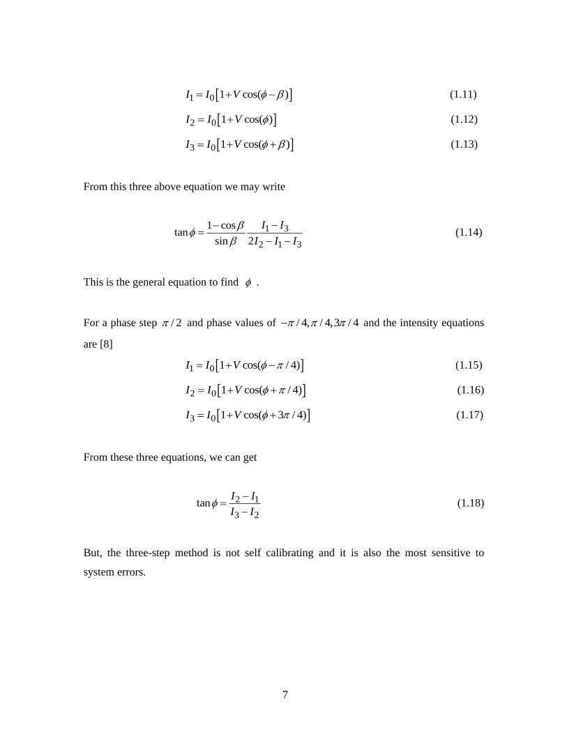
1 0 1 cos( )I I V (1.11)

2 0 1 cos( )I I V (1.12)

3 0 1 cos( )I I V (1.13)

From this three above equation we may write

1 3

2 1 3

1 costan

sin 2

I I

I I I

(1.14)

This is the general equation to find .

For a phase step / 2 and phase values of / 4, / 4,3 / 4 and the intensity equations

are [8]

1 0 1 cos( / 4)I I V (1.15)

2 0 1 cos( / 4)I I V (1.16)

3 0 1 cos( 3 / 4)I I V (1.17)

From these three equations, we can get

2 1

3 2

tanI I

I I

(1.18)

But, the three-step method is not self calibrating and it is also the most sensitive to

system errors.

8

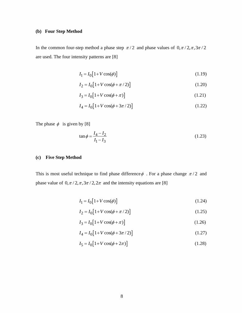
(b) Four Step Method

In the common four-step method a phase step / 2 and phase values of 0, / 2, ,3 / 2

are used. The four intensity patterns are [8]

1 0 1 cos( )I I V (1.19)

2 0 1 cos( / 2)I I V (1.20)

3 0 1 cos( )I I V (1.21)

4 0 1 cos( 3 / 2)I I V (1.22)

The phase is given by [8]

4 2

1 3

tanI I

I I

(1.23)

(c) Five Step Method

This is most useful technique to find phase difference . For a phase change / 2 and

phase value of 0, / 2, ,3 / 2,2 and the intensity equations are [8]

1 0 1 cos( )I I V (1.24)

2 0 1 cos( / 2)I I V (1.25)

3 0 1 cos( )I I V (1.26)

4 0 1 cos( 3 / 2)I I V (1.27)

5 0 1 cos( 2 )I I V (1.28)

9

From this above five equations we get phase as

2 4

3 5 1

2( )tan

2

I I

I I I

(1.29)

In the present work a five-step method as described above is used for the measurement of

the shape of a 3-D object. The five step algorithm is useful as it acts as a self-calibration

for phase shifting and if there is no miss-calibration of phase shifter for 2 phase shift,

then 5 1( )I I .

10

CHAPTER 2

TV HOLOGRAPHIC SYSTEM AND THEORY

2.1. Experimental Arrangement

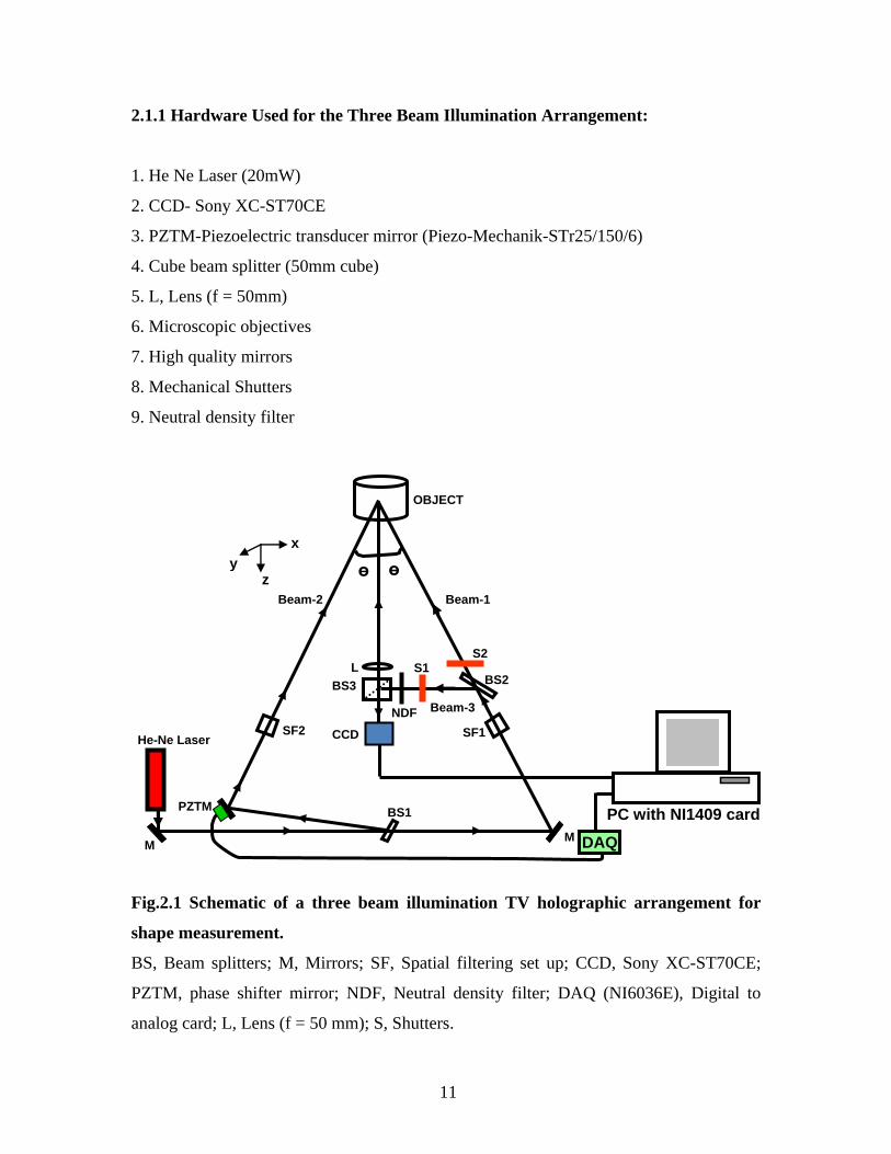
The schematic of the three beam illumination arrangement is shown in Fig.2.1. The

narrow beam from a continuous wave 20mW He-Ne laser is divided into two beams

using a beam splitter (BS1). One beam (Beam-1) falls on a mirror (M) and after reflecting

it passes through a spatial filtering set up (SF1) to expand the beam. Similarly the second

beam (Beam-2) also expanded using the spatial filtering setup (SF2). The diffusely

reflective surface is symmetrically illuminated with two expanded beams (Beam-1 and

Beam-2) inclined at an angle θ with respect to the surface normal. A smooth reference

wave (Beam-3) is added at the CCD plane using a beam splitter (BS2) and a cube beam

splitter ( BS3) in one of the object beam illumination (Beam-1) A lens (f=50mm) is used

to image the object on to the Sony XC-ST70CE CCD. A PZTM Mirror (Piezo-Mechanik

– STr 25/150/6) in Beam-2 is used for introducing the desired phase steps. The PZTM is

interface with a PC with a digital-to-analog card (NI6036E). The neutral density filter

(NDF) in the setup allows to controlling the intensity ratio between the object and

reference beams. The CCD camera is interfaced to a PC with an NI1409 frame grabber

card. The frame grabber is a device that interfaces with a camera to capture and stores a

complete video frame and converts into a digital image. The shutters S1 and S2 in the

setup allow for sequential recording using two beams at a time for shape and the

corresponding object rotation (tilt) measurements. LabVIEW programs have been used

for (i) visualization of real time speckle correlation fringes, and (ii) storing the phase

shifted frames for fringe analysis.

11

2.1.1 Hardware Used for the Three Beam Illumination Arrangement:

1. He Ne Laser (20mW)

2. CCD- Sony XC-ST70CE

3. PZTM-Piezoelectric transducer mirror (Piezo-Mechanik-STr25/150/6)

4. Cube beam splitter (50mm cube)

5. L, Lens (f = 50mm)

6. Microscopic objectives

7. High quality mirrors

8. Mechanical Shutters

9. Neutral density filter

Fig.2.1 Schematic of a three beam illumination TV holographic arrangement for

shape measurement.

BS, Beam splitters; M, Mirrors; SF, Spatial filtering set up; CCD, Sony XC-ST70CE;

PZTM, phase shifter mirror; NDF, Neutral density filter; DAQ (NI6036E), Digital to

analog card; L, Lens (f = 50 mm); S, Shutters.

He-Ne Laser

M

PZTM

S1 S2

BS1

BS3

SF1 SF2

L

CCD

OBJECT

ө ө

x

z y

Beam-1 Beam-2

Beam-3

BS2

NDF

PC with NI1409 card

DAQ M

12

2.1.2 Processing Cards and Supporting Drivers and Software:

1. Frame Grabber Card: NI PCI-1409 - National Instruments

2. IMAQ 3.5.1 Driver and Vision Acquisition software

3. D/A: Digital to analog card- Model No. NI6036E – low cost multifunction i/o &

NI DAQ card, ribbon cable and 68 pin connector block - National Instruments

(NI).

4. LabVIEW 7.1.and Matlab

2.2. Theory for Measurement of Shape and Tilt

TV holography is widely used for the measurement of in-plane (u, v) and out-of-plane

displacement (w) components of a deformation vector L

[1-2]. The optical arrangement

shown in Fig.2.1 plays an important role in extracting the individual displacement

components. The dual beam symmetrical illumination arrangement in the setup using the

illuminating beams, Beam-1 and Beam-2 (Channel-1) allows to study the in-plane

displacement (u) component, while the out-of-plane displacement component using the

Beam-2 and Beam-3 (Channel-2) helps to evaluate the corresponding rotation (tilt) given

to the object for precise measurement of shape of a 3-D object. The in-plane sensitive

configuration (Channel-1) converts the in-plane motion of a curved object due to rotation

of the object into depth variation of a 3-D object (shape) [5-7].

2.1.1 CHANNEL-1: In-plane Sensitive Arrangement for 3-D Surface

Shape (Z) Measurement

For shape measurement we use the symmetrically illuminating object beams (Beam-1

and Beam-2) by blocking the smooth reference wave enters the CCD using the shutter S1

(Fig.2.1). At the CCD plane, the image will consist of the interference of the two

independent, coherent speckle patterns due to each beam as shown in Fig.2.2 (a). The

phase difference at the observation plane can be written as [1-2]

13

1 1 2

2 1

( ). ( , ) ( ). ( , )

( ). ( , )

o ok k L x y k k L x y

k k L x y

(2.1)

where 1k

and 2k

are the propagation vectors in the direction of illumination, and ok

in

the direction observation as shown in figure. ( , , )L u v w

is the displacement component

along x, y and z directions. From Fig.2.2 (a) the terms 1k

, 2k

, 0k

and ( , )L x y

can be

written as [1]

12 ˆˆsin cosk i k

(2.2)

22 ˆˆsin cosk i k

(2.3)

02 ˆk k

(2.4)

ˆˆ ˆ( , )L x y ui vj wk

(2.5)

Inserting these four equations (from Eq. 2.2 to Eq. 2.5) in equation (2.1), we get

14

sinu

(2.6)

Here u gives the in-plane displacement. The in-plane sensitive configuration (Channel-1)

converts the in-plane motion (u) of a curved object due to the rotation ξ of the object into

the depth variation (Z) using the following relation sinu Z Z [5-7]. Hence the

Equation (2.6) for a 3-D object becomes

12

2 sinZ

(2.7)

14

Bright fringes formed when phase difference 1 is equal to integral odd multiple of .

2

2 sinZ m

And 2 sin

mZ

(2.8)

The depth contour interval is governed by 2 sin

Z

The sensitivity of the set up in this configuration is given by / 2 sin . The shape

contour interval sensitivity is dependent on angle θ between the two symmetrically

illuminated object beams with respect to the optical axis (Channel-1). It can be seen from

the equation (2.8) for precise measurement of the shape, we require the (a) angle

between the two symmetrical illumination beams and also (b) rotation/tilt (ξ) given to the

3-D object. The rotation/tilt angle (ξ) can be obtained simultaneously using the setup

shown in Channel-2 (Fig.2.2 (b)) as explained below

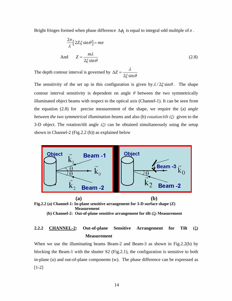
(a) (b) Fig.2.2 (a) Channel-1: In-plane sensitive arrangement for 3-D surface shape (Z)

Measurement

(b) Channel-2: Out-of-plane sensitive arrangement for tilt (ξ) Measurement

2.2.2 CHANNEL-2: Out-of-plane Sensitive Arrangement for Tilt (ξ)

Measurement

When we use the illuminating beams Beam-2 and Beam-3 as shown in Fig.2.2(b) by

blocking the Beam-1 with the shutter S2 (Fig.2.1), the configuration is sensitive to both

in-plane (u) and out-of-plane components (w). The phase difference can be expressed as

[1-2]

15

2 2 0( ). ( , )k k L x y

2

sin cosu w

(2.9)

Since the in-plane component due to the tilt is zero [1-2] and hence the phase change

2 directly related to the object tilt ξ component as

22

(1 cos )

(2.10)

The sensitivity corresponding to tilt given to the object is given by /(1 cos ) .

The rotation and tilt angle obtained from equation (2.10) can used in equation (2.8)

for precise measurement of the shape (Z) of the 3-D object.

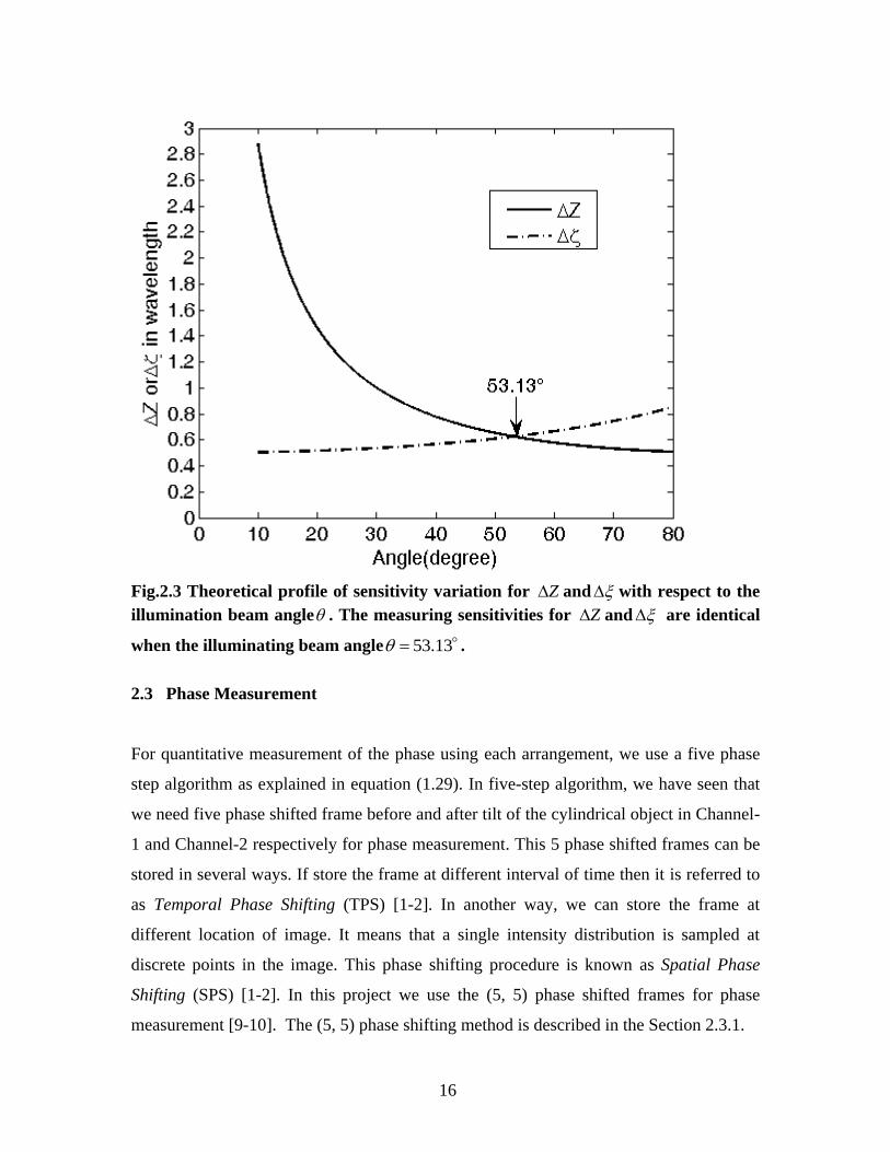
The Equation (2.8) and Equation. (2.10) clearly indicates that the measuring sensitivities

are dependent on the oblique illumination beam angle θ. Fig.2.3 shows the sensitivity

plot between the illumination beam angle θ and the depth Z and the corresponding tilt ξ.

It is interesting to note that Z and the corresponding tilt ξ can be extracted from the setup

with the identical measuring sensitivities when the illumination angle θ is 53.13º (that is

0.6257λ). Hence the three beam illumination arrangement provides a scope for trade-off

between the Z and the corresponding tilt ξ measuring sensitivity.

16

Fig.2.3 Theoretical profile of sensitivity variation for Z and with respect to the

illumination beam angle . The measuring sensitivities for Z and are identical

when the illuminating beam angle 53.13 .

2.3 Phase Measurement

For quantitative measurement of the phase using each arrangement, we use a five phase

step algorithm as explained in equation (1.29). In five-step algorithm, we have seen that

we need five phase shifted frame before and after tilt of the cylindrical object in Channel-

1 and Channel-2 respectively for phase measurement. This 5 phase shifted frames can be

stored in several ways. If store the frame at different interval of time then it is referred to

as Temporal Phase Shifting (TPS) [1-2]. In another way, we can store the frame at

different location of image. It means that a single intensity distribution is sampled at

discrete points in the image. This phase shifting procedure is known as Spatial Phase

Shifting (SPS) [1-2]. In this project we use the (5, 5) phase shifted frames for phase

measurement [9-10]. The (5, 5) phase shifting method is described in the Section 2.3.1.

17

2.3.1 (5, 5) Phase Shifted Algorithm

For phase measurement we store five phase shifted un-deformed frames using the

Channel-1 and Channel-2 respectively. The intensity distribution of the five phase

shifted frames stored from the Channel-1 arrangement is written as [1-2, 9]

2 cos ( 1)2

N O R O RT I I I I N

(2.11)

where N= 1, 2, 3, 4, 5 will give the five phase shifted frames with phase difference 2

. The

speckle phase distribution can be obtained by using the five step algorithm [1] and it is given

by

1 2 4

3 1 5

2( )tan

2

T T

T T T

(2.12)

Here no fringes can be observed, because this interference pattern is a speckle pattern and

the speckle pattern is a granular structure, is not a fringe pattern and is a random

speckle phase.

Similarly the intensity distribution of five phase shifted frame recorded from Channel-1

arrangement in the loaded state of the object is given as [1-2, 9]

12 cos ( 1)2

N O R O RT I I I I N

(2.13)

where 1 is the phase change that cause due to the tilt of the object.

18

The phase distribution 1 can also be obtained by using five step phase shifting

algorithm. This phase distribution is given by [1-2, 9]

1 2 4

1

3 1 5

2( )tan

2

T T

T T T

(2.14)

Similarly no fringe pattern will be seen from the evaluated phase.

Now we subtract the equation (2.12) from the equation (2.14) to obtain the phase 1 ,

which is given below

1 1( )

or 11 12 4 2 4

3 1 53 1 5

2( ) 2( )tan tan

22

T T T T

T T TT T T

(2.15)

The equation (2.15) yields the required phase map fringes. Using the (5, 5) phase shifting

approach, we can completely eliminate the speckle phase term .

A similar expression for the phase 2 corresponding to the tilt measurement can be

obtained from the Channel-2.

The resultant raw phase maps obtained by using the speckle phase shifted frames are

noisy. It is necessary to filter these raw phase maps. Reduction of noise is done by means

of Filtering process. There are some filtering programs available in Matlab and out of

them one can adopt one of available average filter with (5x5) window to smoothen out of

noise. For this filtering we divide the phase map into sine term and cosine term and filter

individually [10].

After filtering we get noise reduced phase map. But this phase map is wrapped phase

map. It means that the phase map is not a continuous phase map, it has 2 phase jump.

19

So, we have to remove this 2 phase jumps and convert into desired continuous phase

function. This process is called unwrapping process of a wrapped phase map. This

unwrapping is done by solution of Poisson‟s equation with a specific form at fast discrete

cosine transformation (DCT) [11-12]. We have used this unwrapping process by DCT in

the Matlab. After unwrapping we convert this unwrapped phase into the shape and the

corresponding object tilt data using the Eq. 2.8 and Eq.2.10 respectively.

The Procedure followed for the speckle fringe analysis is

1. Raw wrapped phase map evaluation from the stored phase shifted frames by using

Channel-1 and Channel-2.

2. Filtering and smoothening to reduced speckle noise.

3. Phase unwrapping using the DCT (2D profile).

4. 3D-profile for (1) shape (z)

(2) Tilt ( ) using the equation 2.8 and equation 2.10 respectively

The experimental results and analysis for the 3-D surface shape measurement using the

three beam illumination TV holographic system is presented in Chapter 3.

20

CHAPTER 3

EXPERIMENTAL RESULTS

The experiments are conducted on a cylindrical object and a stratum of Buddha using the

three beam illumination arrangement shown in Fig.2.1.

3.1. Shape Measurement of a Cylindrical Object

Experiments are carried out with a cylindrical object. To make the surface area

diffusively reflecting we use a white paint sprays (SKD-S2 Spotcheck developer). The

object is placed in a three beam illumination setup shown in Fig.2.1 and imaged onto the

CCD using the 50 mm focal length lens. The illumination beam angle θ used in the

experiment is around 14ο. The phase shifter unit in the setup activated and calibrated to

store the phase shifted frame before and after tilt given to the object.

Using the Channel-1 (in-plane sensitive) and Channel-2 (out-of-plane sensitive) we store

the five phase shifted frames before and after the tilt given to the cylindrical object using

each arrangement in sequential order. For this the LabVIEW 7.1 is used for sequential

storing of the phase shifted frames using the two beams at a time from the three beam

illumination arrangement. The program stores 10 phase shifted frames (before and after

tilt) in each arrangement.

Procedures followed for sequential recording of the phase shifted frames using the

(5, 5) Phase Stepping method:

Procedures for storing the 5 phase shifted frames before and 5 phase shifted frames after

tilting the cylindrical object using the setup (Fig.2.1)

21

1. First the reference Beam-3 is blocked using the shutter S1. The shutter S2 is opened.

This will allow only the two symmetrical illumination object beams (Beam-1 and

Beam-2) as shown in Channel1 (Fig.2.2 (a)) respectively falling on the object. Five

phase shifted frames that represent the initial state of the cylindrical object with two

beams illumination are stored in the computer.

2. Open the Shutter-S1 and block the Beam-1 using the Shutter-S2. This will allow

Channel-2 (Fig.2.2 (b)) (out-of-plane sensitive configuration) functional. Five phase

shifted frames that represent the initial state of the cylindrical object with Cannel-2 in

operation are stored in the computer.

3. Use the same Channel-2 arrangement now the cylindrical object is given a small tilt

and we stored five phase shifted in tilted state of the object in the computer.

4. Final step is to open the Shutter-S2 and block the Beam-1 using the Shutter-S1. This

will allow Channel-1 arrangement functional. The final five phase shifted frames that

represent the tilted state of the cylindrical object using the two beam illumination

setup are stored.

The procedure allows to store the 10 phase shifted frames in each arrangement for fringe

analysis. From the equation (2.7) and equation (2.10) as explained in Chapter 2.2, the

phase difference related to the shape and tilt of the object from each arrangement needs to

be evaluated from the stored phase shifted frames. We have used a (5,5) phase shifting

algorithm [1, 9-10] as explained in Section 2.2.1, Chapter 2 for measurement of the phase

from each arrangement

3.1.1 Channel – 1: 3-D Surface Shape (Z) Measurement

The phases and 1 evaluated from the stored phase shifted frames before and

tilting the object with Channel-1 arrangement (in-plane sensitive configuration) using the

equation (2.12) and the equation (2.14) is shown in Fig.3.1(a) and Fig.3.2(b)

22

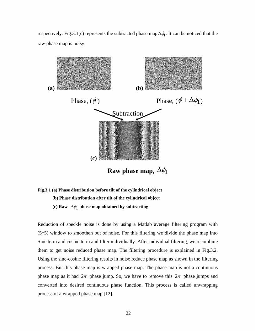
respectively. Fig.3.1(c) represents the subtracted phase map 1 . It can be noticed that the

raw phase map is noisy.

(a) (b)

Phase, ( ) Phase, ( 1 )

Subtraction

(c)

Raw phase map, 1

Fig.3.1 (a) Phase distribution before tilt of the cylindrical object

(b) Phase distribution after tilt of the cylindrical object

(c) Raw 1 phase map obtained by subtracting

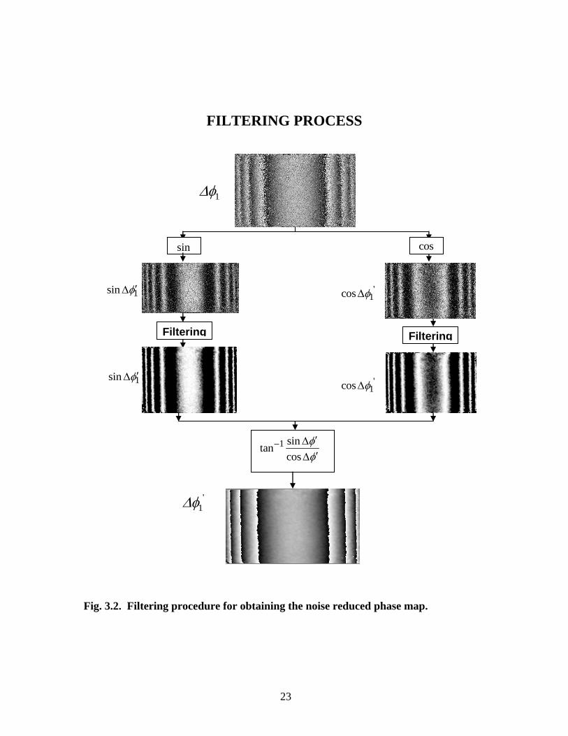
Reduction of speckle noise is done by using a Matlab average filtering program with

(5*5) window to smoothen out of noise. For this filtering we divide the phase map into

Sine term and cosine term and filter individually. After individual filtering, we recombine

them to get noise reduced phase map. The filtering procedure is explained in Fig.3.2.

Using the sine-cosine filtering results in noise reduce phase map as shown in the filtering

process. But this phase map is wrapped phase map. The phase map is not a continuous

phase map as it had 2 phase jump. So, we have to remove this 2 phase jumps and

converted into desired continuous phase function. This process is called unwrapping

process of a wrapped phase map [12].

23

FILTERING PROCESS

Fig. 3.2. Filtering procedure for obtaining the noise reduced phase map.

sin cos

Filtering Filtering

1sin '1cos

'1cos

1

1sin

1 sintan

cos

'1

24

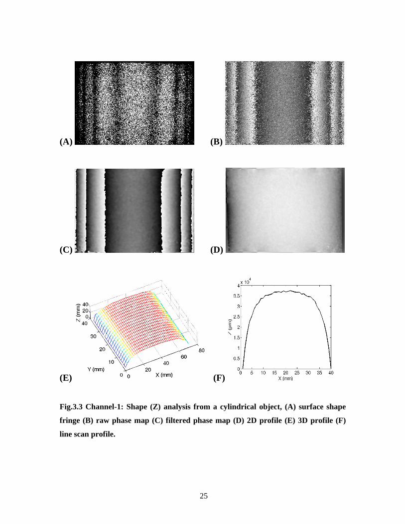
We have used this unwrapping process by DCT in the Matlab. After unwrapping we

convert this unwrapped phase into the shape using the equation 2.8. For precise

measurement of surface shape, we need the corresponding tilt value ξ given to the

cylindrical object. The tilt value ξ measured using the stored phase shifted frames from

the Channel-2 (out-of-plane sensitive arrangement) is explained in the next section. The

measured tilt ξ given to the object is used in equation 2.8 to obtain the shape. The

analysis for 3-D surface shape measurement is shown in Fig. 3.3.

25

(A) (B)

(C) (D)

(E) (F)

Fig.3.3 Channel-1: Shape (Z) analysis from a cylindrical object, (A) surface shape

fringe (B) raw phase map (C) filtered phase map (D) 2D profile (E) 3D profile (F)

line scan profile.

26

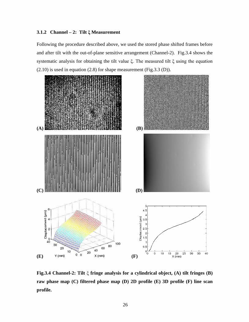
3.1.2 Channel – 2: Tilt ξ Measurement

Following the procedure described above, we used the stored phase shifted frames before

and after tilt with the out-of-plane sensitive arrangement (Channel-2). Fig.3.4 shows the

systematic analysis for obtaining the tilt value ξ. The measured tilt ξ using the equation

(2.10) is used in equation (2.8) for shape measurement (Fig.3.3 (D)).

(A) (B)

(C) (D)

(E) (F)

Fig.3.4 Channel-2: Tilt ξ fringe analysis for a cylindrical object, (A) tilt fringes (B)

raw phase map (C) filtered phase map (D) 2D profile (E) 3D profile (F) line scan

profile.

27

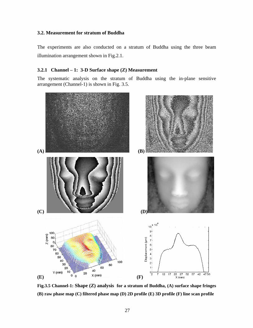
3.2. Measurement for stratum of Buddha

The experiments are also conducted on a stratum of Buddha using the three beam

illumination arrangement shown in Fig.2.1.

3.2.1 Channel – 1: 3-D Surface shape (Z) Measurement

The systematic analysis on the stratum of Buddha using the in-plane sensitive

arrangement (Channel-1) is shown in Fig. 3.5.

(A) (B)

(C) (D)

(E) (F)

Fig.3.5 Channel-1: Shape (Z) analysis for a stratum of Buddha, (A) surface shape fringes

(B) raw phase map (C) filtered phase map (D) 2D profile (E) 3D profile (F) line scan profile

28

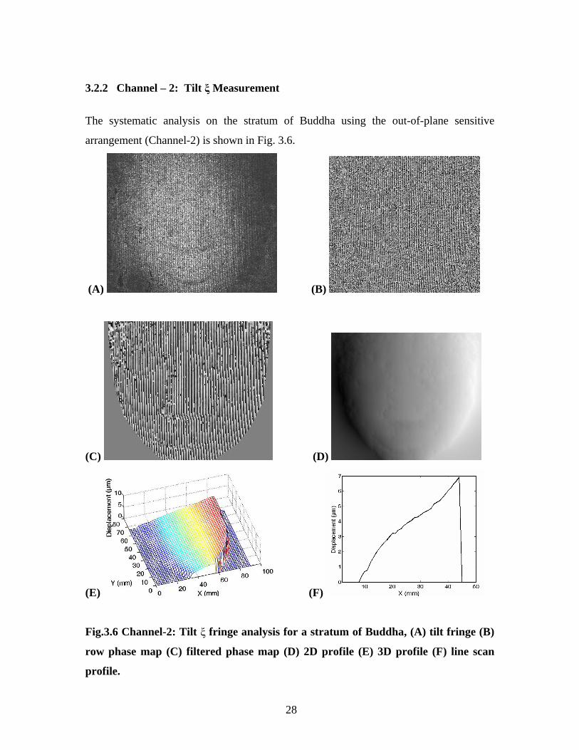
3.2.2 Channel – 2: Tilt ξ Measurement

The systematic analysis on the stratum of Buddha using the out-of-plane sensitive

arrangement (Channel-2) is shown in Fig. 3.6.

(A) (B)

(C) (D)

(E) (F)

Fig.3.6 Channel-2: Tilt ξ fringe analysis for a stratum of Buddha, (A) tilt fringe (B)

row phase map (C) filtered phase map (D) 2D profile (E) 3D profile (F) line scan

profile.

29

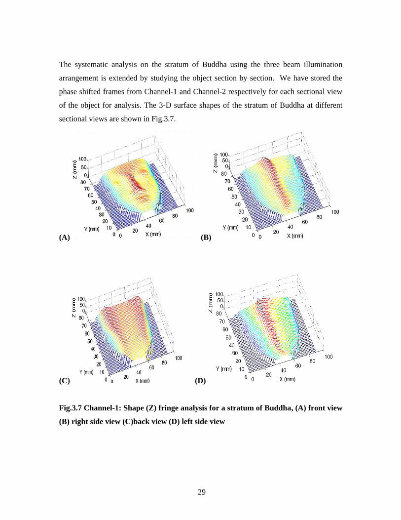
The systematic analysis on the stratum of Buddha using the three beam illumination

arrangement is extended by studying the object section by section. We have stored the

phase shifted frames from Channel-1 and Channel-2 respectively for each sectional view

of the object for analysis. The 3-D surface shapes of the stratum of Buddha at different

sectional views are shown in Fig.3.7.

(A) (B)

(C) (D)

Fig.3.7 Channel-1: Shape (Z) fringe analysis for a stratum of Buddha, (A) front view

(B) right side view (C)back view (D) left side view

30

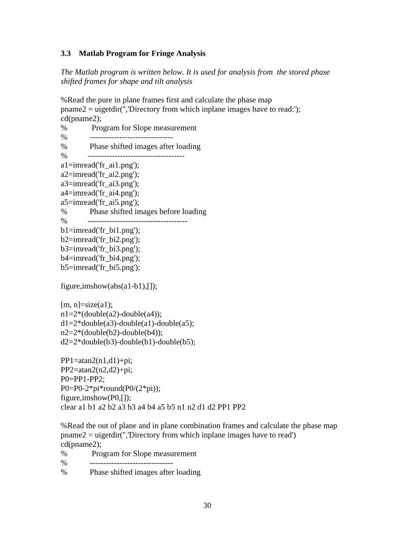
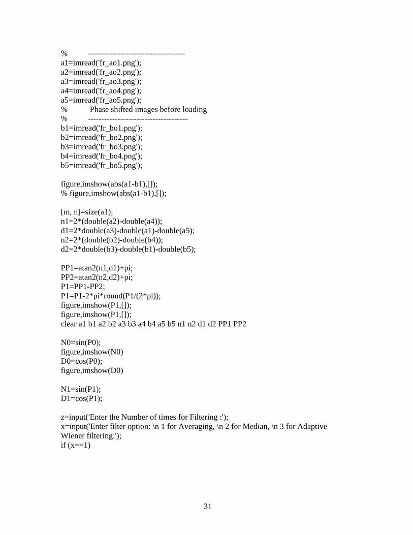
3.3 Matlab Program for Fringe Analysis

The Matlab program is written below. It is used for analysis from the stored phase

shifted frames for shape and tilt analysis

%Read the pure in plane frames first and calculate the phase map

pname2 = uigetdir('','Directory from which inplane images have to read:');

cd(pname2);

% Program for Slope measurement

% -------------------------------

% Phase shifted images after loading

% ------------------------------------

a1=imread('fr_ai1.png');





% Phase shifted images before loading

% -------------------------------------

b1=imread('fr_bi1.png');





figure,imshow(abs(a1-b1),[]);

[m, n]=size(a1);

n1=2*(double(a2)-double(a4));

d1=2*double(a3)-double(a1)-double(a5);

n2=2*(double(b2)-double(b4));

d2=2*double(b3)-double(b1)-double(b5);

PP1=atan2(n1,d1)+pi;


P0=PP1-PP2;

P0=P0-2*pi*round(P0/(2*pi));

figure,imshow(P0,[]);

clear a1 b1 a2 b2 a3 b3 a4 b4 a5 b5 n1 n2 d1 d2 PP1 PP2

%Read the out of plane and in plane combination frames and calculate the phase map

pname2 = uigetdir('','Directory from which inplane images have to read')

cd(pname2);

% Program for Slope measurement

% -------------------------------

% Phase shifted images after loading

31

% ------------------------------------

a1=imread('fr_ao1.png');





% Phase shifted images before loading

% -------------------------------------

b1=imread('fr_bo1.png');





figure,imshow(abs(a1-b1),[]);

% figure,imshow(abs(a1-b1),[]);

[m, n]=size(a1);

n1=2*(double(a2)-double(a4));

d1=2*double(a3)-double(a1)-double(a5);

n2=2*(double(b2)-double(b4));

d2=2*double(b3)-double(b1)-double(b5);



P1=PP1-PP2;

P1=P1-2*pi*round(P1/(2*pi));



clear a1 b1 a2 b2 a3 b3 a4 b4 a5 b5 n1 n2 d1 d2 PP1 PP2

N0=sin(P0);

figure,imshow(N0)

D0=cos(P0);

figure,imshow(D0)

N1=sin(P1);

D1=cos(P1);

z=input('Enter the Number of times for Filtering :');

x=input('Enter filter option: \n 1 for Averaging, \n 2 for Median, \n 3 for Adaptive

Wiener filtering:');

if (x==1)

32

% Averaging Filter

% ------------------

y=input('Enter the length of the averaging window \n(3 or 5 or 7):');

p=fspecial('average',[y y]);

for k=1:z

N0=sin(P0);

D0=cos(P0);

N0=imfilter(N0,p);

D0=imfilter(D0,p);

P0=atan2(N0,D0);

N1=sin(P1);

D1=cos(P1);

N1=imfilter(N1,p);

D1=imfilter(D1,p);

P1=atan2(N1,D1);

end

elseif(x==2)

% Median filtering

% ------------------

y=input('Enter the window length \n(3 or 5 or 7):');

for k=1:z

N0= medfilt2(N0,[y,y]);

D0= medfilt2(D0,[y,y]);

N1= medfilt2(N1,[y,y]);

D1= medfilt2(D1,[y,y]);

end

P0=atan2(N0,D0);

P1=atan2(N1,D1);

elseif(x==3)

% Adaptive Wiener filtering

% ---------------------------

y=input('Enter the window length \n(3 or 5 or 7):');

for k=1:z

N0= wiener2(N0,[y,y]);

D0= wiener2(D0,[y,y]);

N1= wiener2(N1,[y,y]);

D1= wiener2(D1,[y,y]);

end

P0=atan2(N0,D0);

P1=atan2(N1,D1);

end

clear N0 N1 D0 D1 k y z x p

% Masking

33

% ---------------

A1=input('Enter \n 0 for no masking, \n 1 for masking:');

if(A1==1)

M=P0.*0;

M=roipoly(P0);

%M=1-M;

%M=1-M;

P0=P0.*M;

P1=P1.*M;

end



% unwrapping

% ---------------

for i =1:m

for j= 1:n

if (j==n)

a=0;

else

a=P0(i,j+1)-P0(i,j);

end

if (a>=pi)

a=a-2*pi;

elseif(a<=-pi)

a=a+2*pi;

end

if (j==1)

b=0;

else

b=P0(i,j)-P0(i,j-1);

end

if (b>=pi)

b=b-2*pi;

elseif(b<=-pi)

b=b+2*pi;

end

if (i==m)

c=0;

else

c=P0(i+1,j)-P0(i,j);

end

if (c>=pi)

c=c-2*pi;

elseif(c<=-pi)

c=c+2*pi;

end

34

if (i==1)

d=0;

else

d=P0(i,j)-P0(i-1,j);

end

if (d>=pi)

d=d-2*pi;

elseif(d<=-pi)

d=d+2*pi;

end

R(i,j)=a-b+c-d;

clear a b c d;

end

end

r=dct2(R);

clear R;

for k=1:m

for l=1:n

q(k,l)=r(k,l)/(2*cos(pi*k/m)+2*cos(pi*l/n)-4);

end

end

clear r;

Q0=2*idct2(q);

clear q;

figure,imshow(Q0,[]);

for i =1:m

for j= 1:n

if (j==n)

a=0;

else

a=P1(i,j+1)-P1(i,j);

end

if (a>=pi)

a=a-2*pi;

elseif(a<=-pi)

a=a+2*pi;

end

if (j==1)

b=0;

else

b=P1(i,j)-P1(i,j-1);

end

if (b>=pi)

b=b-2*pi;

elseif(b<=-pi)

35

b=b+2*pi;

end

if (i==m)

c=0;

else

c=P1(i+1,j)-P1(i,j);

end

if (c>=pi)

c=c-2*pi;

elseif(c<=-pi)

c=c+2*pi;

end

if (i==1)

d=0;

else

d=P1(i,j)-P1(i-1,j);

end

if (d>=pi)

d=d-2*pi;

elseif(d<=-pi)

d=d+2*pi;

end

R(i,j)=a-b+c-d;

clear a b c d;

end

end

r=dct2(R);

clear R;

for k=1:m

for l=1:n

q(k,l)=r(k,l)/(2*cos(pi*k/m)+2*cos(pi*l/n)-4);

end

end

clear r;

Q1=2*idct2(q);

clear q;

figure,imshow(Q1,[]);

angle=input('Enter the angle of illumination:\n angle=');

angle=angle*pi/180;

lam=0.6328;

W=Q1*lam/(4*pi*cos(angle));

W=W-min(min(W));

x=input('Enter the x value:\x value=');

T=(max(max(W))-min(min(W)))/(x);

S=Q0*lam/(4*pi*sin(T)*sin(angle));

36

S=S-min(min(S));

[m,n]=size(W);

for i =1:m

for j = 1:n

if((rem(i,15)==0) & (rem(j,15)==0))

k=i/15;

l=j/15;

if (A1==1)

U1(k,l)=M(i,j)*W(i,j);

else

U1(k,l)=W(i,j);

end

end

end

end

G=input('Enter the magnification:\G =');

X=0:1.8:15*G*50;

Y=0:1.8:15*G*37;

figure,mesh(X,Y,U1)

figure,mesh(X,Y,flipud(U1))

for i =1:m

for j = 1:n

if((rem(i,15)==0) & (rem(j,15)==0))

k=i/15;

l=j/15;

if (A1==1)

U2(k,l)=M(i,j)*S(i,j);

else

U2(k,l)=S(i,j);

end

end

end

end

figure,mesh(X,Y,U2*10^(-3))

figure,mesh(X,Y,flipud(U2*10^(-3)))

37

CONCLUSIONS

A three beam illumination TV holographic system is developed and demonstrated for 3-D

surface profile (shape) analysis. The arrangement combines an in-plane sensitive

arrangement with an out-of-plane sensitive arrangement for simultaneous measurement

of the shape and the corresponding tilt angle given to the object. The basic theory of

fringe formation in a three beam illumination arrangement considering two beams at a

time is described. For fringe analysis we have used the sequential procedure for recording

the phase shifting frames in each configuration. We have used the software in LabVIEW

for storing the frames and Matlab programs for fringe analysis. The development of the

system along with the experimental results on a cylindrical object and a stratum of

Buddha are presented.

38

REFERENCE

1. P. K. Rastogi, Ed., Digital speckle pattern interferometry and related techniques.

John Wiley and Sons, New York, 2001.

2. N. Krishna Mohan, Speckle Methods and Applications, In Toru Yoshizawa, Ed.

Handbook of Optical Metrology: Principles and Applications. Chapter 8, pp. 241-

262. CRC Press, Boca Raton, Florida, 2009.

3. E.B. Hack, R. Kästle, and U. Sennhauser, “Additive-Subtractive two-wavelength

ESPI contouring by using a synthetic wavelength phase shift,” Applied Optics, 37,

2591-2597 (1998).

4. Saldner, H. O., N.-E. Molin, and N. Krishna Mohan (1994) Simultaneous

measurement of out-of-plane displacement and slope change by electronic holo-

shearography. Proceedings of 10th

international Conference of Experimental

mechanics, Lisbon, Portugal, 337-341.

5. A.R.Ganesan and R.S. Sirohi, “New method of contouring using digital speckle

pattern interferometry (DSPI),” Proc.SPIE 954, 327-332 (1985).

6. C. Joenathan, B. Pfister, and H. J. Tiziani, “Contouring by electronic speckle

pattern interferometry employing dual beam illumination,” Applied Optics, 29,

1905-1911 (1990).

7. N. Krishna Mohan, A.Svanbro, M. Sjodahl and N.E.Molin, “Dual-beam

symmetric illumination observation TV holographic system for measurements”

Optical Engineering, 40, 2780-2787 (2001).

8. R. S. Sirohi and M P. Kothiyal “Optical components, Systems and Measurement

techniques, Marcel Dekker Inc., New York, 1991.

9. P. Hariharan, B.F. Oreb, and T. Eiju, “Digital phase shifting interferometry – a

simple error-compensating phase calculation algorithm,” Applied Optics, 26,

2504-2506 (1987).

10. Basanta Bhaduri, Sanjit K. Debnath, N. Krishna Mohan and M.P. Kothiyal, “A

comparative study of phase shifting algorithms for speckle and speckle shear

fringe analysis”, 12-15 December 2005, Dehradun, Article No:OP-OIM3. pp-1-6

39

11. D.C Ghiglia and L.A. Romero, “Robust Two-dimensional weighted and un-

weighted phase unwrapping that uses fast transformation and iterative methods”,

J. Opt. Soc. Am. A, 11, pp. 107-117 (1994).

12. D.C. Ghiglia and M.D. Pritt, Two-dimensional phase unwrapping: Theory,

algorithms and software. John Wiley and Sons, New York, 1998.

matlab program related optics project

Documents