matlab for pattern recognition - página principalsadoc/machinelearning/matlab-sadoc.pdf · matlab...
TRANSCRIPT
MATLAB FOR PATTERN RECOGNITION
MIN 720 – Pattern Classification for Biomedical Applications, Prof. Dr. Neşe Yalabık
05/04/2011

How Much Do We Know?
Anybody who has never used MATLAB?

Outline
An Introduction to MATLAB Generation of Random Data Basic Statistical Functions Parameter/Density Estimation Functions Classification/Clustering Functions MATLAB Toolboxes for Pattern
Recognition

MATLAB Environment
Workspace: Variables defined so far. Command History Command Window Editor Plot Window Current Directory: Start by setting the current directory
to the directory that you are working. Generally, it is where your files are.
Workspace Window

LOOKFOR & HELP
LOOKFOR: Type ‘lookfor smth’ to learn the name of functions that are related to ‘smth’.
HELP: Type ‘help function_name’ to learn how that function works, its inputs and outputs.

Expressions Variables:
No need to make type declarations or dimension statements
When Matlab encounters a new variable name, it automatically creates the variable and allocates the appropriate amount of storage.
Example:
>> num_students = 25
Creates a 1-by-1 matrix named num_students and stores the value 25 in its single element
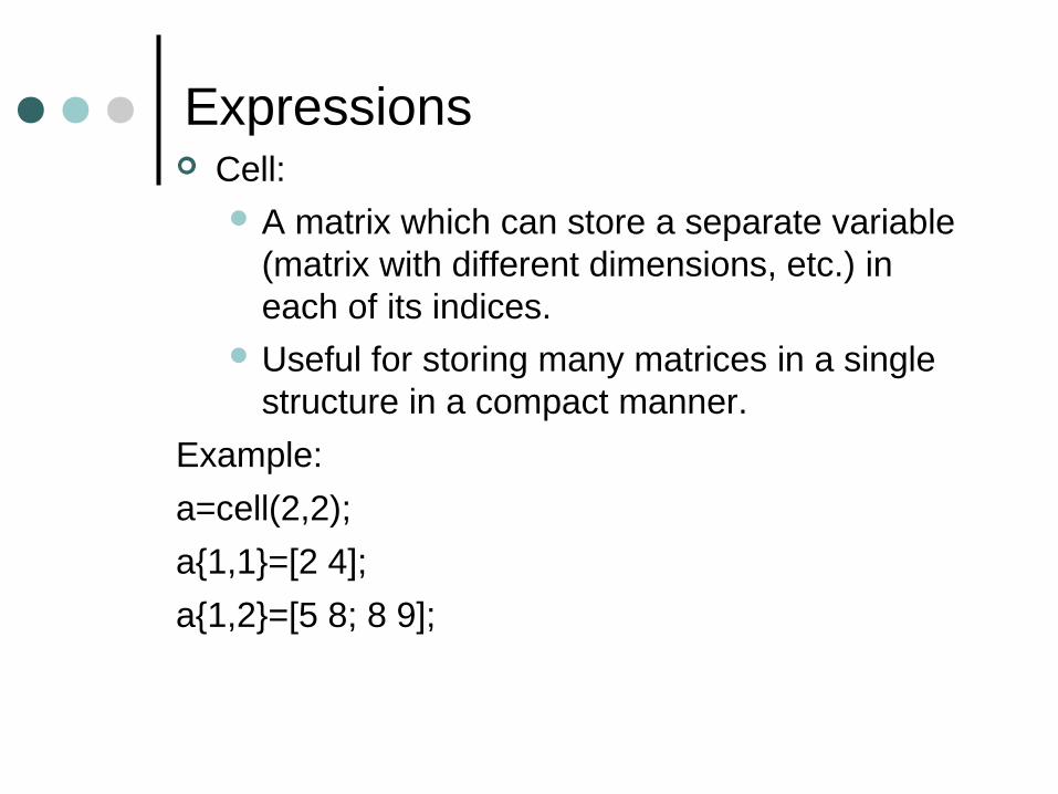
Expressions Cell:
A matrix which can store a separate variable (matrix with different dimensions, etc.) in each of its indices.
Useful for storing many matrices in a single structure in a compact manner.
Example:
a=cell(2,2);
a{1,1}=[2 4];
a{1,2}=[5 8; 8 9];
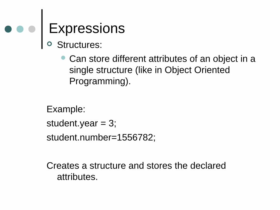
Expressions Structures:
Can store different attributes of an object in a single structure (like in Object Oriented Programming).
Example:
student.year = 3;
student.number=1556782;
Creates a structure and stores the declared attributes.

Functions Standard elemantary mathematical functions; abs,
sqrt, exp, sin …
For a list of elemantary mathematical functions type
>> help elfun
For a list of more advanced mathematical and matrix functions type
>>help specfun
>>help elmat
Most of the functions are overloaded.
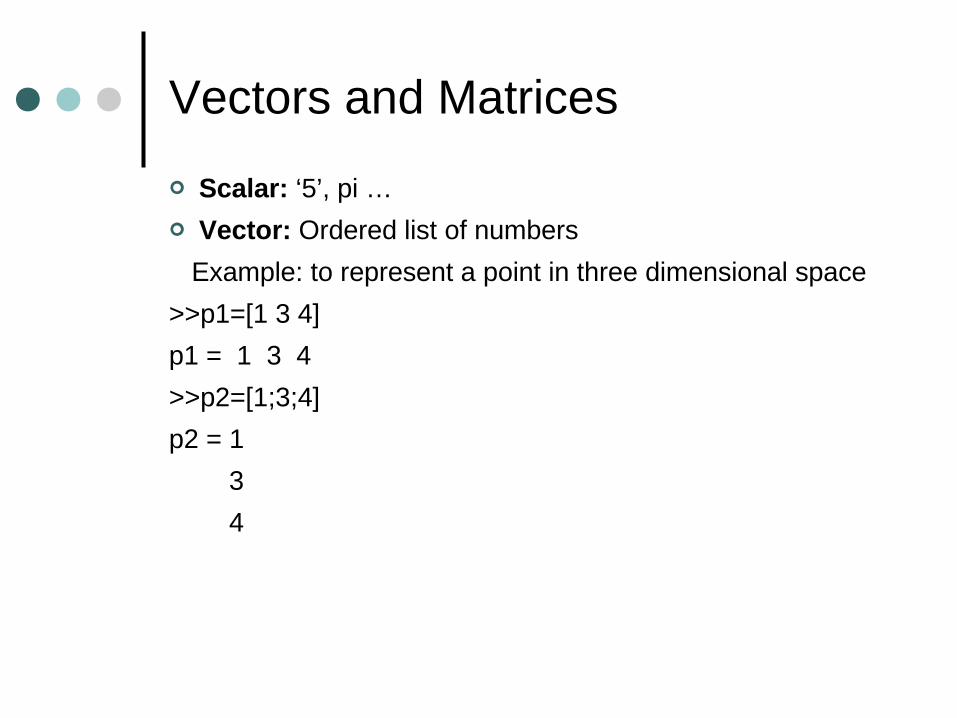
Vectors and Matrices
Scalar: ‘5’, pi …
Vector: Ordered list of numbers
Example: to represent a point in three dimensional space
>>p1=[1 3 4]
p1 = 1 3 4
>>p2=[1;3;4]
p2 = 1
3
4

Accessing a Vector
Access to the elements of vectors
>>p1(1)
ans =
1

Creating Matrices Matrices:>> a = [ 1 2 2 1 ] a = 1 2 2 1 >> b= [1; 2; 2; 1]b=
1221
>>c=zeros(1,2);c= 0 0>>d=ones(1,3);d= 1 1 1
Creating Matrices from Vectors
It is possible to create matrices from row or column vectors, as long as all of the vectors being used to create the matrix have the same number of elements.
Examples…

Accessing a Matrix Accessing element of a matrix
>>a=[2 4; 5 8];
>>a(1,:)
2 4
>>a(:,2)
5
8 Accessing subset of a matrix
>>b=[1 2 3 ; 4 5 6; 7 8 9];
>>b(2:3,2:3)
5 6
8 9

Matrix Operations Matrix operations like, (for matrices “x” and “y”)
Determinant of a matrix (det(x)) Inverse of a matrix (x^-1) or inv(x) Transpose of a matrix (x’) Element by element multiplication(x.*y),
division(x./y) Matrix multiplication(x*y), division(x/y),
summation(x+y), subtraction(x-y) … are defined in MATLAB.
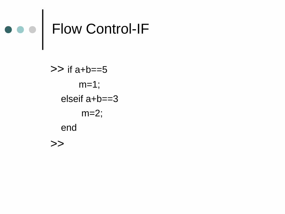
Flow Control-IF
>> if a+b==5
m=1;
elseif a+b==3
m=2;
end
>>

Flow Control-Switch
>> switch (n) case 0
M=0case 1
M=1otherwise
M=2end

Loops
For/End
a = [ 0.8 0.1; 0.2 0.9 ; 0.4 0.6]
>> for i = 1:1:3
x(i,:) = a(i,:).*i
end

While/End
a=3; ax=0
while a==3
ax=ax+2
if ax>50
a=4
end
end
Avoid using Loops in Matlab.
M-Files: Scripts And Functions
Scripts: Do not accept input arguments or return output arguments. They operate on data in the workspace.
Functions: can accept input arguments and return output arguments. Internal variables are local to the function.
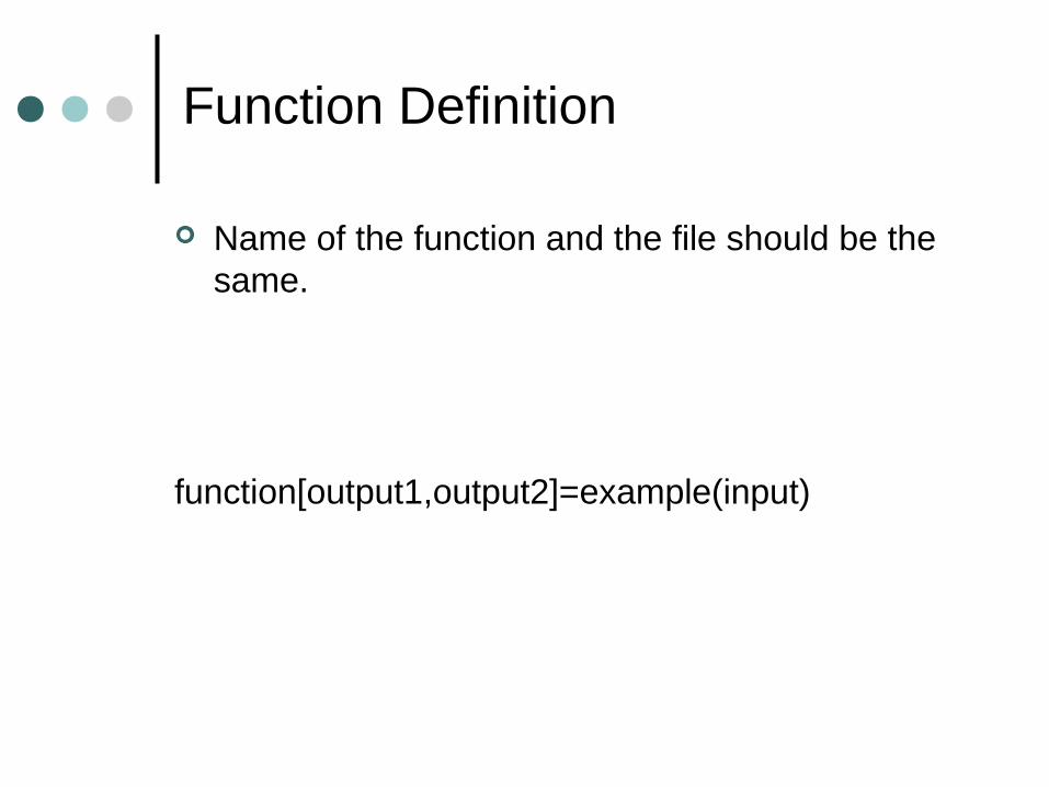
Function Definition
Name of the function and the file should be the same.
function[output1,output2]=example(input)
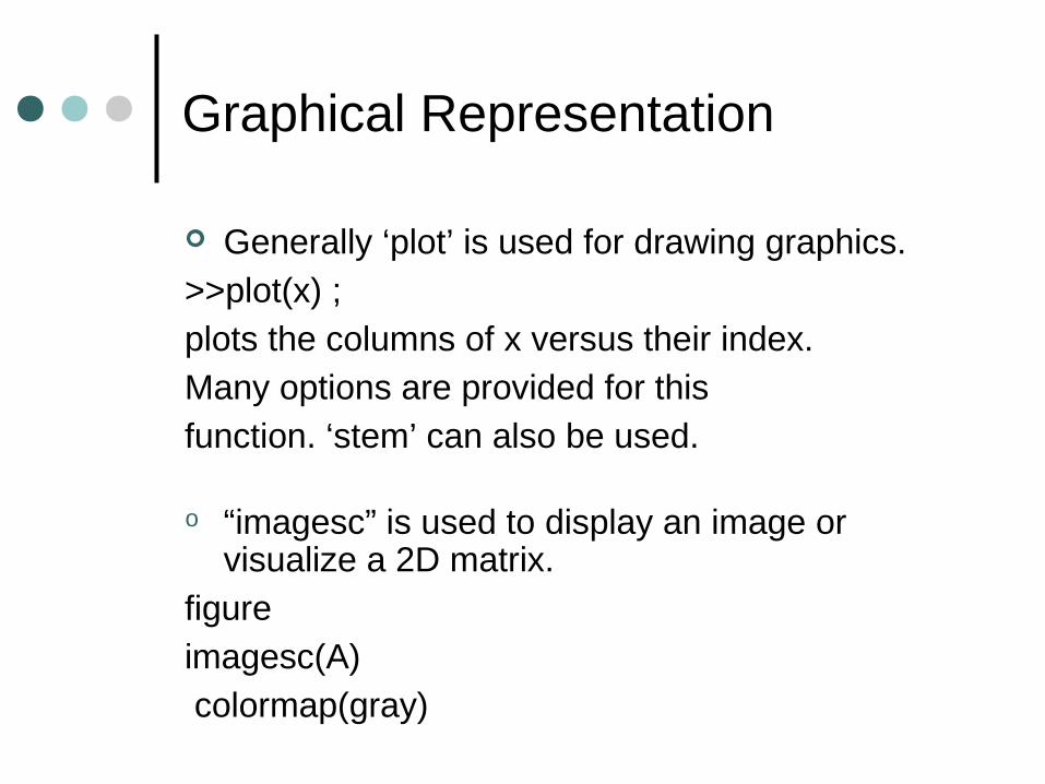
Graphical Representation
Generally ‘plot’ is used for drawing graphics.>>plot(x) ;plots the columns of x versus their index.Many options are provided for thisfunction. ‘stem’ can also be used.
o “imagesc” is used to display an image or visualize a 2D matrix.
figureimagesc(A) colormap(gray)

Read & Write Files
Load, Save,Saveas Textread … There are many other functions for file
operations. Check File I/O part in Mathwork’s Help.

Generating Random Data
There are many functions for generating random samples from a desired distribution with the specified parameters.
random('name',a,b,c,....) creates a matrix with the specified dimensions whose entries are samples drawn from the specified distribution.
>> x1 = random('unif',0,1,2,4)
0.8003 0.4218 0.7922 0.6557
0.1419 0.9157 0.9595 0.0357

Generating Random Data
normrnd(mu,sigma,m,n) creates a mxn matrix whose entries are samples drawn from a normal distribution with specified parameters.
>> normrnd(50,10,2,5)
45.674 51.253 38.535 61.891 53.272
33.344 52.876 61.909 49.623 51.746 exprnd(mu,m,n) creates a mxn matrix from an
exponential distribution.
>>exprnd(30,2,3)
13.1593 12.4551 37.1646
6.0277 32.1909 32.2592

Generating Random Data
•Sample points from a multivariate Gaussian • Standard deviation of 3 in roughly the lower left-upper right direction and of 1 in the orthogonal direction. • Variances of x and y do not fully describe the distribution. 2×2 covariance matrix needed;• The directions of the arrows correspond to the eigenvectors of this covariance matrix and their lengths to the square roots of the eigenvalues.
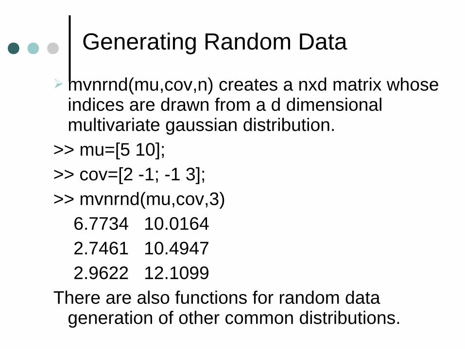
Generating Random Data
mvnrnd(mu,cov,n) creates a nxd matrix whose indices are drawn from a d dimensional multivariate gaussian distribution.
>> mu=[5 10];>> cov=[2 -1; -1 3];>> mvnrnd(mu,cov,3) 6.7734 10.0164 2.7461 10.4947 2.9622 12.1099There are also functions for random data
generation of other common distributions.

Likelihood Evaluation Functions
They calculate likelihood for a specific distribution in a given point.
normpdf(x,mu,sigma)
>> normpdf(4,5,1)
0.2420 exppdf(x,mu)
>>exppdf(10,20)
0.0303 (betapdf( ), mvnpdf( ), etc.)

Basic Statistical Functions
Functions for calculating the descriptive statistics of distributions.
mean(x) returns the mean value of a 1D matrix.
>>x=[2 8 4];>> mean(x) 4.6667 Std(x) returns the standard deviation (with
Bessel’s correction(correction factor n/(n-1))std(x) 3.0551

Basic Statistical Functions
var(x) returns the variance (with Bessel’s correction)
>> var(x) 9.3333
median(x) returns the sample of the distribution which is in the middle rank when samples are ordered.
>>median(x) 4
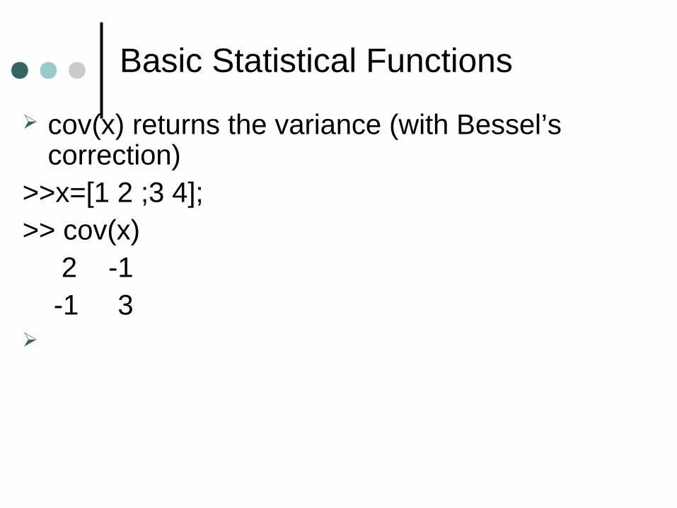
Basic Statistical Functions
cov(x) returns the variance (with Bessel’s correction)
>>x=[1 2 ;3 4];>> cov(x) 2 -1 -1 3
Distance/Metric Functions
mahal(y,x) returns the Mahalanobis distance of the data points(rows) of y to the distribution characterized by the samples(rows) of x.
>>x=[2 3; 4 7 ; 1 5];>> y=[2 7];>> mahal(y,x) 2.3333 pdist(x) returns the Euclidean distance between
pairs of data(rows) points of x.>> pdist(x) 4.4721 2.2361 3.6056

Distance/Metric Functions
pdist(x,distance) can be used to find the distance between pairs of data of x with the specified distance metric.
>> pdist(x,'cityblock') 6 3 5 norm(x) returns the norm of a matrix(or vector).>>norm(x) 10.0906

Parameter Estimation Functions
normfit(x) returns the mean and standard deviation of the data that is assumed to be originated from normal distribution.
>> x=[3 2 6 4 7 3];>>[mu_est,sig_est]=normfit(x)mu_est = 4.1667sig_est = 1.9408
Parameter Estimation Functions
expfit(x) returns the mean of the data that is assumed to be originated from exponential distribution.
>>expfit(x) 4.1667
There are similar functions for other commonly used distributions. The confidence intervals(with adjustable confidence) may also be obtained for the estimates.

Parameter Estimation Functions
mle(x,’distribution’,’dist’) returns the maximum likelihood (ML) estimate of the parameters that is assumed to be originated from the specified distribution by ‘dist’.
>>mle(x,'distribution','normal') 4.1667 1.7717>> mle(x,'distribution','gamma') 5.6322 0.7398
When it is used as mle(x)(with no distribution specification), normal distribution is assumed.
Density Estimation Functions
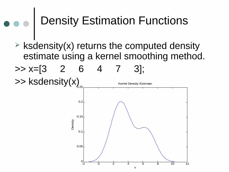
ksdensity(x) returns the computed density estimate using a kernel smoothing method.
>> x=[3 2 6 4 7 3];>> ksdensity(x)
-2 0 2 4 6 8 10 120
0.05
0.1
0.15
0.2
0.25
x
Density
Kernel Density Estimate
Density Estimation Functions
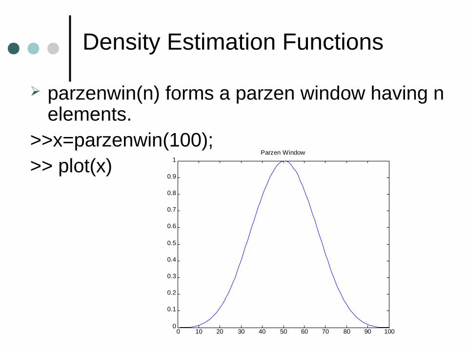
parzenwin(n) forms a parzen window having n elements.
>>x=parzenwin(100);>> plot(x)
0 10 20 30 40 50 60 70 80 90 1000
0.1
0.2
0.3
0.4
0.5
0.6
0.7
0.8
0.9
1Parzen Window
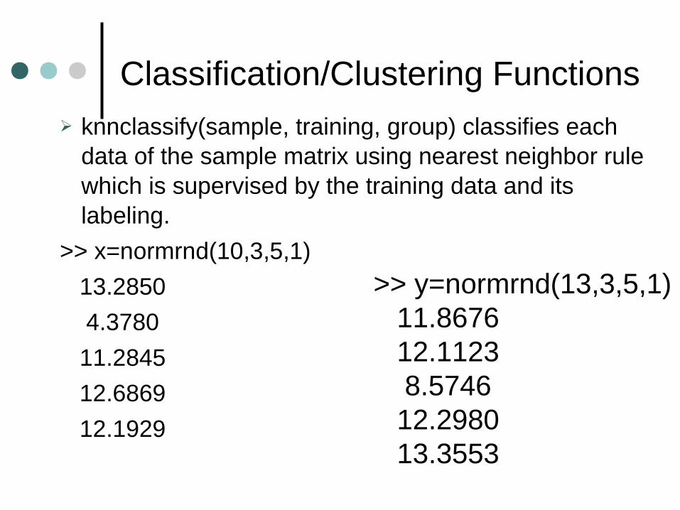
Classification/Clustering Functions knnclassify(sample, training, group) classifies each
data of the sample matrix using nearest neighbor rule which is supervised by the training data and its labeling.
>> x=normrnd(10,3,5,1)
13.2850
4.3780
11.2845
12.6869
12.1929
>> y=normrnd(13,3,5,1) 11.8676 12.1123 8.5746 12.2980 13.3553
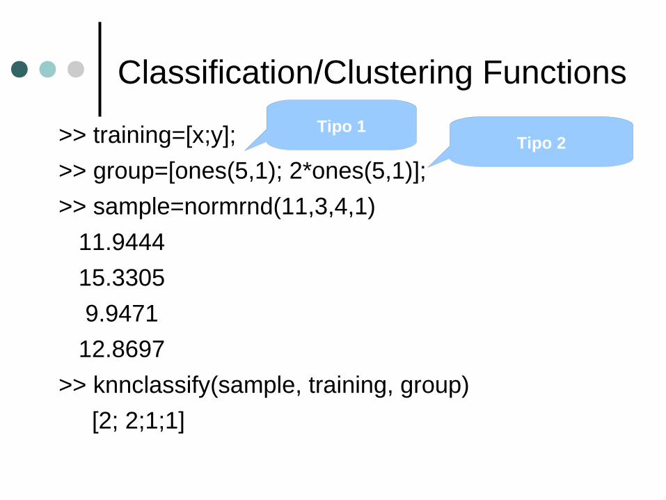
Classification/Clustering Functions
>> training=[x;y];
>> group=[ones(5,1); 2*ones(5,1)];
>> sample=normrnd(11,3,4,1)
11.9444
15.3305
9.9471
12.8697
>> knnclassify(sample, training, group)
[2; 2;1;1]
Tipo 1Tipo 2

Classification/Clustering Functions
knnclassify(sample, training, group,k) classifies each data using k-nearest neighbor rule.
>>knnclassify(sample, training, group,3)
[2;1;2;1]
Note that classification result changes. knnclassify(sample, training, group,k,distance)
performs classification using the specified distance metric (default is euclidean distance.).

Classification/Clustering Functions
kmeans(x,k) clusters the data into k classes using k means clustering algorithm.
>>kmeans(training,2)
2;2;1;2;2;1;1;1; 1; 2 kmeans function can also be used with other
distance metrics(kmeans(x,k,’distance’,’dist’).
>> kmeans(training,2,'distance','cityblock')
1;1;2;1;1; 2;2; 2; 2;1

Classification/Clustering Functions
classify(sample,training,group) classifies the sample data into classes using the training dataset labeled with group. It performs discriminant analysis.
>> classify(sample,training,group)
[2;2;1;2] The type of discriminant function to be used can be
adjusted.
>> classify(sample,training,group,'quadratic')
[2;1;2;2] Classifier using
discriminant analysis

Classification/Clustering Functions
The priors of the classes can be incorporated into classification.
>> prior=[0.1 0.9];
>>classify(sample,training,group,'quadratic',prior)
[2;2;2;2]
>> prior=[0.9 0.1];
>> classify(sample,training,group,'quadratic',prior)
[1;1;1;1] The choice of priors is critical.

Classification/Clustering Functions
clusterdata(x,cutoff) clusters the data using a hierarchical cluster tree. cutoff is a parameter to adjust the number of clusters to be formed at the end (0<cutoff<2).
>> x=normrnd(20,2,5,1);
>> y=normrnd(30,2,5,1);
>> z=[x;y];
>> t=clusterdata(z,1)
[4;4;2;1;1;3;3;3;3;3]

Classification/Clustering Functions
>> t=clusterdata(z,1.2)
[1;1;1;1;1;1;1;1;1;1]
The distance metric to be used can be changed and the maximum number of clusters to be formed can be specified.

Classification/Clustering Functions
voronoi(x,y) forms the voronoi diagram for the datasets x and y.
>> x=mvnrnd([20 ; 15],[2 0 ;0 2],10);
>> y=mvnrnd([23 ; 12],[2 0 ;0 2],10);
>> voronoi(x,y)
13 14 15 16 17 18 19 20 21 2210
15
20
25Voronoi Diagram

Classification/Clustering Functions
clustergram(x) draws the dendogram of the dataset x. The similar and distant datasets are visualized.
>> z=[x;y];
>> clustergram(z)
2 1
8 1 4 7 616101418 3 213201519 912 51711
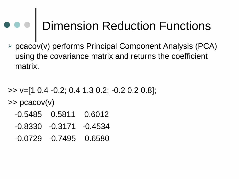
Dimension Reduction Functions
pcacov(v) performs Principal Component Analysis (PCA) using the covariance matrix and returns the coefficient matrix.
>> v=[1 0.4 -0.2; 0.4 1.3 0.2; -0.2 0.2 0.8];
>> pcacov(v)
-0.5485 0.5811 0.6012
-0.8330 -0.3171 -0.4534
-0.0729 -0.7495 0.6580

Dimension Reduction Functions
PCA can also be performed with princomp(x) directly from the data.
>>princomp(x)
0.6668 0.7453
0.7453 -0.6668
MATLAB Toolboxes
A Toolbox is a collection of m-files developed to perform computation on a particular domain.
Ex:Animation toolbox(Developing scientific animations)
Some toolboxes are present inside MATLAB but some are not embedded. They are available on the Internet.

MATLAB Toolboxes
Neural Networks Toolbox:
Includes tools for designing, implementing, visualizing and simulating neural networks.
Statistics Toolbox:
Provides tools for modeling and analyzing data, simulating systems, developing statistical algorithms, learning and teaching statistics.
MATLAB Toolboxes
PRTools Toolbox:
Includes algorithms for data generation, training classifiers, features selection, density estimation, feature extraction, cluster analysis.
Statistical Pattern Recognition Toolbox:
It provides users with procedures for discriminant functions, feature extraction, density estimation, support vector machines, visualization, regression, etc..

MATLAB Toolboxes
Fuzzy Logic Toolbox Classification Toolbox Clustering Toolbox ClusterPack Toolbox GHSOM Toolbox HMM Toolbox HMMBOX Toolbox LPSVM Toolbox NSVM Toolbox
MATLAB Toolboxes
PCNN Toolbox SDH Toolbox SOM Toolbox SSVM Toolbox SVM Toolbox SVM Classifier Toolbox Bioinformatics Toolbox

END
Thank you for listening.
Any Questions or Comments ??