mathematischesforschungsinstitutoberwolfach · the presentations of abels, asai, bellettini, bothe,...
TRANSCRIPT

Mathematisches Forschungsinstitut Oberwolfach
Report No. 07/2010
DOI: 10.4171/OWR/2010/07
New Directions in Simulation, Control and Analysis forInterfaces and Free Boundaries
Organised byCharles M. Elliott, Warwick
Yoshikazu Giga, TokyoMichael Hinze, Hamburg
Vanessa Styles, Brighton
January 31st – February 6th, 2010
Abstract. The field of mathematical and numerical analysis of systems ofnonlinear partial differential equations involving interfaces and free bound-aries is a flourishing area of research. Many such systems arise from mathe-matical models in material science, fluid dynamics and biology, for examplephase separation in alloys, epitaxial growth, dynamics of multiphase fluids,evolution of cell membranes and in industrial processes such as crystal growth.The governing equations for the dynamics of the interfaces in many of theseapplications involve surface tension expressed in terms of the mean curvatureand a driving force. Here the forcing terms depend on variables that are solu-tions of additional partial differential equations which hold either on the in-terface itself or in the surrounding bulk regions. Often in applications of thesemathematical models, suitable performance indices and appropriate controlactions have to be specified. Mathematically this leads to optimization prob-
lems with partial differential equation constraints including free boundaries.Because of the maturity of the field of computational free boundary problemsit is now timely to consider such control problems.
In order to carry out design, control and simulation of such problems in-teraction is required between distinct mathematical fields such as analysis,modeling, computation and optimization. By bringing together leading ex-perts and young researchers from these separate fields we intended to developnovel research directions in applied and computational mathematics. The aimof the workshop here was to focus on emerging new themes and developmentsin these fields and to establish and extend links between them.
Mathematics Subject Classification (2000): MSC: 35-XX, 49-XX, 65-XX IMU: 11, 16, 17.
Introduction by the Organisers

254 Oberwolfach Report 07/2010
The meeting was attended by 53 participants from Austria, Belgium, China,France, Germany, Great Britain, Japan, Portugal, Spain and the United States,with expertise from three main areas: optimal control of partial differential equa-tions, modeling involving free boundary problems and mathematical and numeri-cal analysis of free boundary problems. Apart from discussing current problems,techniques and issues across the differing communities the focus of the workshopwas set on developing the necessary analytical and numerical techniques requiredto successfully tackle new emerging classes of problems related to the followingthemes:
(1) Computational and analytical approaches to interfaces and free bound-aries,
(2) Control and optimization of interfaces and free boundaries,(3) Numerical treatment and control of surface partial differential equations.
The presentations of Abels, Asai, Bellettini, Bothe, Garcke, Giga, Kohsaka, Ni-ethammer, Roger and Santosa concerned analytical approaches to interfaces andfree boundaries. While Feng, Kornhuber, Nurnberg, Pozzi, Reusken, A. Schmidt,Stoll, and Tobiska gave talks on numerical approaches to interfaces and free bound-aries. Control and optimization with focus on interfaces and free boundaries wasthe subject of the talks of Bernauer, Casas, Deckelnick, Gunther, Hintermuller,Raymond, S. Schmidt, Siebert, Vierling and Yan. Elliott gave a survey talk onthe treatment of surface partial differential equations with surface finite elements,and Voigt, in his talk, introduced a diffuse-interface approach for the numericaltreatment of coupled bulk/surface partial differential equations. Finally, Sprekels,in his talk, reported on the state of the art of mathematical and technical achieve-ments in Czochralski crystal growth. This method may be considered a modelapplication containing many of the topics considered within the workshop.
To offer young researchers a stage for presenting their research, a young re-searcher session was organized on Wednesday evening where the Heizaemon HondaScholar Asai together with the Oberwolfach Leibniz Graduate Students Bernauer,Gunther, S. Schmidt, and Vierling took this opportunity and gave talks on theircurrent research results.
Surveys and articles concerning mathematical and numerical approaches to in-terfaces and free boundary problems may be found in the conference proceedings[5, 6, 2, 8]. The level set approach to related problems of optimal design aresurveyed in [3]. The book [1] contains theoretical results for optimal control ofvariational inequalities. Modern mathematical concepts of control and optimiza-tion with partial differential equation constraints are developed in the book [7].Also we mention a survey of numerical methods for interface evolution involvingcurvature, [4]. Finally we remark that many recent references concerning the issuesof the workshop are provided at the end of the each extended abstract.Acknowledgement: The organizers would like to thank Professor Karl HeinzHoffmann for many fruitful discussions in the run-up to the application for thisOberwolfach workshop.

Simulation, Control and Analysis for Interfaces and Free Boundaries 255
References
[1] V. Barbu Optimal control of Variational Inequalities Pitman Research Notes in Mathematics100 Pitman Boston London Melbourne (1984).
[2] A. Bossavit, A. Damlamian and M. Fremond (editors) Free Boundary Problems: applicationsand theory Pitman Research Notes in Mathematics 121 Pitman Boston London Melbourne(1985).
[3] M. Burger and S. Osher A survey on level set methods for inverse problems and optimal
design Euro. J. Appl. Math. 16 (2005) 263–301.[4] K.P. Deckelnick, G. Dziuk and C.M. Elliott Computation of Geometric PDEs and Mean
Curvature Flow Acta Numerica (2005) 139–232.[5] C.M. Elliott and J.R. Ockendon Weak and variational methods for moving boundary prob-
lems. Pitman Research Notes in Mathematics 59 Pitman Boston London Melbourne (1982).[6] A. Fasano and M. Primicerio (editors) Free Boundary Problems, Theory Applications Pit-
man Research Notes in Mathematics 79 Pitman Boston London Melbourne (1983).[7] M. Hinze, R. Pinnau, M. Ulbrich, S. Ulbrich Optimization with PDE constraints MMTA
23, Springer (2009).[8] K.H. Hoffman and J. Sprekels (editors) Free Boundary Problems, Theory and Applications
Pitman Research Notes in Mathematics 186 Pitman Boston London Melbourne (1990).


Simulation, Control and Analysis for Interfaces and Free Boundaries 257
Workshop: New Directions in Simulation, Control and Analysisfor Interfaces and Free Boundaries
Table of Contents
T. Asai, M. Bernauer, A. Gunther, S. Schmidt, M. VierlingYoung researcher Session . . . . . . . . . . . . . . . . . . . . . . . . . . . . . . . . . . . . . . . . . 261
Helmut AbelsSharp and Diffuse Interface Models for Two-Phase Flows of ViscousIncompressible Fluids . . . . . . . . . . . . . . . . . . . . . . . . . . . . . . . . . . . . . . . . . . . . 262
Giovanni Bellettini (joint with M. Novaga and G. Orlandi)Minimal timelike lorentzian submanifolds as limits of singularly perturbedwave equations . . . . . . . . . . . . . . . . . . . . . . . . . . . . . . . . . . . . . . . . . . . . . . . . . . 265
Dieter Bothe (joint with Jan Pruss)Transport processes at fluidic interfaces . . . . . . . . . . . . . . . . . . . . . . . . . . . . 266
Eduardo CasasOptimal Control of PDEs. Topics and Methods . . . . . . . . . . . . . . . . . . . . . . 268
Klaus Deckelnick (joint with C.M. Elliott and V. Styles)An arrival time inverse problem for the eikonal equation . . . . . . . . . . . . . . 269
Charlie Elliott (joint with Bjoern Stinner)Surface finite elements for two phase geometric biomembranes . . . . . . . . . 271
Xiaobing Feng (joint with Andreas Prohl, Haijun Wu)Exponential-free a priori and a posteriori error estimates for finiteelement approximations of diffuse interface equations for surfaceevolution . . . . . . . . . . . . . . . . . . . . . . . . . . . . . . . . . . . . . . . . . . . . . . . . . . . . . . . 272
Harald Garcke (joint with Stefan Schaubeck)The Stefan Problem with anisotropic Gibbs–Thomson law . . . . . . . . . . . . . 275
Yoshikazu Giga (joint with Robert V. Kohn, Courant–NYU)On scale–independent extinction time estimates for total variation flows 278
M. Hintermuller (joint with I. Kopacka)Optimal Control of Variational Inequalties: Stationarity; -ies andNumerics . . . . . . . . . . . . . . . . . . . . . . . . . . . . . . . . . . . . . . . . . . . . . . . . . . . . . . . 279
Yoshihito Kohsaka (joint with Harald Garcke, Kazuo Ito)Motion of phase boundaries by geometric evolution equations . . . . . . . . . . 283
Ralf Kornhuber (joint with Carsten Graser, Uli Sack)Nonsmooth Schur Newton Methods for Nonsmooth Saddle PointProblems . . . . . . . . . . . . . . . . . . . . . . . . . . . . . . . . . . . . . . . . . . . . . . . . . . . . . . . 286

258 Oberwolfach Report 07/2010
Barbara Niethammer (joint with A. Munch, D. Peschka)Self-similar rupture in thin films with slip . . . . . . . . . . . . . . . . . . . . . . . . . . 287
Robert Nurnberg (joint with John W. Barrett, Harald Garcke)Parametric approximation of geometric evolution equations andapplications to the modelling of snowflake growth . . . . . . . . . . . . . . . . . . . . 288
Takeshi OhtsukaLevel set method for spiral crystal growth and surface evolution . . . . . . . . 291
P. PozziFEM approximation of the anisotropic mean curvature flow in highercodimension . . . . . . . . . . . . . . . . . . . . . . . . . . . . . . . . . . . . . . . . . . . . . . . . . . . . 295
Jean-Pierre RaymondStabilization of a fluid – structure model . . . . . . . . . . . . . . . . . . . . . . . . . . . . 295
Arnold Reusken (joint with P. Esser, J. Grande, S. Groß, M. Olshanskii)Numerical methods for surfactant transport in two-phase incompressibleflows . . . . . . . . . . . . . . . . . . . . . . . . . . . . . . . . . . . . . . . . . . . . . . . . . . . . . . . . . . 298
Matthias Roger (joint with L. Mugnai)The Allen–Cahn action functional and forced mean curvature flow . . . . . 301
Fadil Santosa (joint with Selim Esedoglu)An Analysis of a Bar Code Deconvolution Problem . . . . . . . . . . . . . . . . . . 302
Alfred Schmidt (joint with Eberhard Bansch, Thilo Moshagen, and JordiPaul)Finite element simulation of solid-liquid phase transitions with a freemelt surface . . . . . . . . . . . . . . . . . . . . . . . . . . . . . . . . . . . . . . . . . . . . . . . . . . . . 304
Stephan Schmidt (joint with Volker Schulz)Large Scale Aerodynamic Shape Optimization . . . . . . . . . . . . . . . . . . . . . . . 307
Kunibert G. Siebert (joint with Kristina Kohls and Arnd Rosch)Analysis of Adaptive Finite Elements for Control Constrained OptimalControl Problems . . . . . . . . . . . . . . . . . . . . . . . . . . . . . . . . . . . . . . . . . . . . . . . . 308
Jurgen Sprekels (joint with Wolfgang Dreyer (WIAS Berlin), P.-E. Druet(WIAS Berlin), O. Klein (WIAS Berlin), F. Troltzsch (TU Berlin), I.Yousept (TU Berlin))Technical and Mathematical Problems in the Czochralski Growth of SingleCrystals . . . . . . . . . . . . . . . . . . . . . . . . . . . . . . . . . . . . . . . . . . . . . . . . . . . . . . . . 312
Martin Stoll (joint with Lavinia Sarbu, Luise Blank)Preconditioning for Allen-Cahn variational inequalities with non-localconstraints . . . . . . . . . . . . . . . . . . . . . . . . . . . . . . . . . . . . . . . . . . . . . . . . . . . . . 314
Lutz Tobiska (joint with Sashikumaar Ganesan)Finite element methods for interface flows with surfactants . . . . . . . . . . . 315

Simulation, Control and Analysis for Interfaces and Free Boundaries 259
Ningning Yan (joint with Duan Wang and Ruo Li)Anisotropic adaptive finite element methds for interface problems . . . . . . 317
Axel Voigt (joint with Sebastian Aland, Andreas Ratz, John Lowengrub)A diffuse-interface approach for solving coupled bulk/surface PDEs incomplex evolving domains . . . . . . . . . . . . . . . . . . . . . . . . . . . . . . . . . . . . . . . . 319


Simulation, Control and Analysis for Interfaces and Free Boundaries 261
Abstracts
Young researcher Session
T. Asai, M. Bernauer, A. Gunther, S. Schmidt, M. Vierling
Tomoro Asai: On the smoothing effect for higher order curvature flow equa-tions We constructed a local unique smooth solution starting from a rough initialcurve for higher order curvature flow equations including the surface diffusion flowand the Willmore flow. The initial curvature is allowed to be discontinuous. Forthis purpose we develop an abstract theory for quasilinear parabolic equationsbased on the theory of analytic semigroups. We estimate lower order terms in acareful way which leads a strong smoothing effect of higher order curvature flowequations.
Martin K. Bernauer (joint with Roland Herzog & Karl Kunisch): Opti-mal Control of the Two-Phase Stefan Problem in Level Set Formulation Motionplanning problems for the two-phase Stefan problem are considered. A level setrepresentation of the moving interface is used. First order optimality conditionsare derived using shape calculus. The approximation of the forward and adjointsystems relies on the X-FEM and discontinuous Galerkin schemes. Numericalexamples are included.
Andreas Gunther (joint with M.H. Tber): A goal-oriented adaptive Moreau-Yosida algorithm for control- and state-constrained elliptic optimal control prob-lems We consider adaptive finite elements for distributed optimal control prob-lems governed by elliptic partial differential equations. Of particular interest isthe tailored design of goal-oriented adaptive meshes under additional control- andstate-constraints. The latter ones are regularized by a Moreau-Yosida penaliza-tion. Throughout our investigations we use piecewise linear finite elements for thestate variable while the control is not discretized. This technique in particularresults in the absence of control residuals in error representations. Our findingsare confirmed by numerical experiments.
Stephan Schmidt (joint with Volker Schulz): Large Scale Aerodynamic ShapeOptimization The talk presents the problem of aerodynamic shape optimizationas a free boundary problem. First, a very brief overview on shape optimizationis given. Next, incompressible fluids are considered. The gradient in Hadamardform is derived for a general incompressible Navier-Stokes problem. Afterwards,the shape Hessian is analyzed and found to have an operator symbol similar tothe Dirichlet-to-Neumann map. The talk concludes with the optimization of anOnera M6 flying wing using the compressible Euler equations to model the fluid.Due to using the Hadamard form of the gradient, a very large scale morphing ofshapes is possible.
Morten Vierling: An optimal order error bound for state constrained optimalcontrol problems We consider the variational discretization of a linear–quadraticoptimal control problem with pointwise control and state constraints. In order toallow for a Frechet smooth norm, the problem is reformulated by means of the

262 Oberwolfach Report 07/2010
reflexive space W 1,p(Ω) instead of C(Ω). The discretization of the state equationyields a family of perturbed optimal control problems, whose solutions can becomputed numerically. Assuming a Slater condition, we apply an implicit mul-tifunction theorem to the first order necessary conditions to proof a bound onthe perturbation error for these solutions. In the special case of an elliptic stateequation in Ω ⊂ R2 undergoing a simple finite element discretization we obtainconvergence of order O(h).
Sharp and Diffuse Interface Models for Two-Phase Flows of ViscousIncompressible Fluids
Helmut Abels
We consider a two-phase flow of two viscous incompressible Newtonian fluidsof the same density filling a domain Ω ⊆ Rd, d = 2, 3. In classical models theinterface between both fluids is modeled as a (d − 1)-dimensional surface Γ(t).– Such a model will be called sharp interface model in the following. – Thesurface energy associated to the interface is σHd−1(Γ(t)), where Hd−1 denotesthe (d − 1)-dimensional Hausdorff measure and σ is a (constant) surface tensioncoefficient. The presence of a surface energy causes an extra contribution to theinner forces/the stress tensor, which is proportional to the mean curvature of theinterface and described by the Young-Laplace law (7) below.
On the other hand in so-called diffuse interface model for such a two-phaseflow a partial mixing of the macroscopically immiscible fluids in a small interfacialregion is assumed in the model. Additionally, diffusion of both components istaken into account. This leads to a coupled Navier-Stokes/Cahn-Hilliard system,which is capable to describe the evolution of droplet formation and collision duringthe flow consistently and reads as follows:
∂tv + v · ∇v − div(ν(c)Dv)︸ ︷︷ ︸inner friction
+∇p = −ε div(∇c⊗∇c)︸ ︷︷ ︸surface tension
(1)
div v = 0(2)
∂tc+ v · ∇c = m∆µ(3)
µ =δEεδc
= −ε∆c+ ε−1φ′(c)(4)
Here v is the mean velocity, Dv = 12 (∇v +∇vT ), p is the pressure, c is an order
parameter related to the concentration of the fluids (e.g. the concentration differ-ence or the concentration of one component), µ is a chemical potential, and Ω is asuitable bounded domain. Moreover, ν(c) > 0 is the viscosity of the mixture, ε > 0is a (small) parameter, which will be related to the “thickness” of the interfacialregion, m > 0 is a mobility coefficient, and φ = Φ′ for some suitable energy densityΦ. The latter model first appeared in [9] with the name “model H”. A rigorousderivation was given in [8].

Simulation, Control and Analysis for Interfaces and Free Boundaries 263
The system is dissipative and sufficiently smooth solution satisfy
d
dtE(c(t), v(t)) = −
∫
Ω
ν(c)|Dv|2 dx−∫
Ω
m|∇µ|2 dx
where E(c(t), v(t)) = Eε(c(t)) +12
∫Ω|v(t)|2 dx, and
Eε(c) =ε
2
∫
Ω
|∇c(x)|2 dx+ ε−1
∫
Ω
Φ(c(x)) dx
describes the energy of the mixture. Here Φ is a double well potential as e.g.Φ(c) = 1
8 (1− c2)2 if c = c1 − c2 is the difference of the mass concentrations.For the mathematical analysis it is essential that both the interface thickness ε
and the mobility m are positive. Under this assumption and suitable assumptionson Φ, the domain and the initial conditions, one can prove the existence of weaksolutions of (1)-(4) in two and three space dimension. Furthermore, strong uniquesolutions exist in two dimensions globally in time and in three dimensions locally intime. Moreover, for large times any weak solution becomes regular and convergesto a solution of the associated stationary system. We refer to [3] for these resultsand further references. In the case ε > 0 and m = 0 existence of weak solutionsis an open problem and so far only short-time existence of strong solutions wasshown, cf. [5].
In applications the parameter ε > 0 is often very small. Therefore a rigorousunderstanding of the limit ε → 0 and the relation to classical sharp interfacemodels is of interest. But the limit system as ε → 0 depends on the choice ofthe scaling of m = m(ε). We expect that, if m(ε) →ε→0 m0 ≥ 0 and c is theconcentration of one fluid, then the limit system is
∂tv + v · ∇v − div(ν±Dv) +∇p = 0 in Ω±(t)(5)
div v = ∆µ = 0 in Ω±(t)(6)
−[n · (ν±Dv − pI)
]= σHn on Γ(t)(7)
V = n · v|Γ(t) −m0[n · ∇µ] on Γ(t)(8)
[v] = 0, µ|Γ(t)= σH on Γ(t)(9)
Here [.] denotes the jump of a function across the interface Γ(t). In the casem0 = 0, the equations for the chemical potential µ decouple from the rest and thesystem coincides with the classical sharp interface model. In the casem0 > 0 it wasshown that weak solutions of (1)-(4) converge (modulo subsequences) to varifoldsolutions of (5)-(9) in the sense of [6]. In the case m0 = 0 convergence was shownby formally matched asymptotics in [12] and it was observed numerically in [10]for some scalings of m(ε).
In the case m0 > 0 existence of weak solutions for large times was shown in[4]. In the case m0 = 0 this is an open problem. So far only short time existenceof strong solutions and existence of varifold solutions globally in time are known,cf. [7, 13], [1, 2], respectively. In order to obtain weak solutions using methodsfrom geometric measure theory, it is essential that sufficiently smooth solutions of

264 Oberwolfach Report 07/2010
(5)-(9) satisfy
d
dtE(v(t),Γ(t)) = −
∫
Ω
ν(χ)|Dv|2 dx−m0
∫
Ω
|∇µ|2 dx
where E(v(t),Γ(t)) = 12‖v(t)‖22+σHd−1(Γ(t)). In the case m0 > 0 this gives some
control of µ and the curvature of the interface Γ(t), which is sufficient to apply aresult by Schatzle [11] and to obtain weak solutions.Conclusion: Comparing diffuse and sharp interface models it is important torealize that there are two new parameters ε > 0, which measure the interfacethickness, and m > 0, which is a mobility coefficient. In particular, since m > 0,new diffusion effects occur in comparison with the classical sharp interface model,which corresponds to the case ε = m = 0. More precisely, in the case m = 0, theinterface is just transported by mean velocity of the mixture v, while in the casem > 0 the evolution of the interface is given by a (non-local) transport-diffusionequation. Therefore the choice of m = m(ε) > 0 influences the behavior of thediffuse interface model a lot and the scaling of m(ε) as ε→ 0 influences the limitsystem. Moreover, we note that in the casem > 0 new effects like Ostwald ripeningoccur, which was observed numerically. On the other hand the existence of globalweak solutions was only shown in the case m > 0 (both for ε > 0 and ε = 0).In this case the energy estimate provides an estimate of the chemical potentialµ, which gives some control of the (“diffuse”) curvature of the interface. Thiscontrol is essential for the construction of global weak solutions. Therefore in thecase m > 0 the system has much better analytical properties. (It is a completelyparabolic system in this case.) But choosing m = m(ε) > 0 new phenomenarelated to diffusion in the system occur, which still have to be understood morerigorously.
References
[1] H. Abels. On generalized solutions of two-phase flows for viscous incompressible fluids.Interfaces Free Bound., 9:31–65, 2007.
[2] H. Abels. On the notion of generalized solutions of two-phase flows for viscous incompressiblefluids. RIMS Kokyuroku Bessatsu, B1:1–15, 2007.
[3] H. Abels. On a diffuse interface model for two-phase flows of viscous, incompressible fluidswith matched densities. Arch. Rat. Mech. Anal., 194(2):463–506, 2009.
[4] H. Abels and M. Roger. Existence of weak solutions for a non-classical sharp interface modelfor a two-phase flow of viscous, incompressible fluids. Ann. Inst. H. Poincare Anal. NonLineaire, 26:2403–2424, 2009.
[5] H. Abels and Y. Terasawa. Non-homogeneous navier-stokes systems with order-parameterdependent stresses. Preprint, Max Planck Institute for Mathematics in the Sciences, No.19/2009, to appear in Math. Math. Methods Appl. Sci., 2009.
[6] X. Chen. Global asymptotic limit of solutions of the Cahn-Hilliard equation. J. DifferentialGeom., 44(2):262–311, 1996.
[7] I. V. Denisova and V. A. Solonnikov. Solvability in Holder spaces of a model initial-boundaryvalue problem generated by a problem on the motion of two fluids. Zap. Nauchn. Sem.Leningrad. Otdel. Mat. Inst. Steklov. (LOMI), 188(Kraev. Zadachi Mat. Fiz. i Smezh. Vo-prosy Teor. Funktsii. 22):5–44, 186, 1991.
[8] M. E. Gurtin, D. Polignone, and J. Vinals. Two-phase binary fluids and immiscible fluidsdescribed by an order parameter. Math. Models Methods Appl. Sci., 6(6):815–831, 1996.

Simulation, Control and Analysis for Interfaces and Free Boundaries 265
[9] P.C. Hohenberg and B.I. Halperin. Theory of dynamic critical phenomena. Rev. Mod. Phys.,49:435–479, 1977.
[10] D. Jacqmin. Calculation of two-phase Navier-Stokes flows using phase-field modeling. J.Comput. Phys., 155(1):96–127, 1999.
[11] R. Schatzle. Hypersurfaces with mean curvature given by an ambient Sobolev function. J.Differential Geom., 58(3):371–420, 2001.
[12] V. N. Starovoıtov. A model of the motion of a two-component fluid taking into accountcapillary forces. Prikl. Mekh. Tekhn. Fiz., 35(6):85–92, 1994.
[13] N. Tanaka. Global existence of two phase nonhomogeneous viscous incompressible fluid flow.Comm. Partial Differential Equations, 18(1-2):41–81, 1993.
Minimal timelike lorentzian submanifolds as limits of singularlyperturbed wave equations
Giovanni Bellettini
(joint work with M. Novaga and G. Orlandi)
I have described a recent convergence result [2] as ǫ → 0+ of solutions of thehyperbolic problems
(1) utt −∆u+1
ǫ2∇W (u) = 0.
Hereu : R× Rn → Rk, n ≥ 1, k = 1, 2,
and W (u) is a suitable potential vanishing only on the unit circle if k = 2 andon ±1 if k = 1, for instance W (u) = 1
4 (1 − |u|2)2 if n ≤ 4 and k = 2. Ourstarting point was a computation made by Neu in [8] where he showed, using aformal argument and assuming k = 1, that there are solutions of (1) which takethe constant values ±1 out of a transition region of thickness ǫ, provided such aregion is close to a timelike lorentzian minimal surface (of codimension one), alsocalled classical string.
Given a solution uǫ to (1) a relevant quantity to be analyzed in the limit ǫ→ 0+
is the rescaled lagrangian density
ℓǫ(uǫ) := ck(ǫ)
(−|uǫt|2 + |∇uǫ|22
+W (uǫ)
ǫ2
)where ck(ǫ) :=
ǫ if k = 1,
1| log ǫ| if k = 2.
Our convergence result shows that ℓǫ(uǫ) concentrates on a k-codimensional setas ǫ → 0+, which is a timelike lorentzian stationary varifold. This theorem isobtained under rather strong assumptions (see [2] for the details) and its proof isbased on a strategy used by Ambrosio and Soner [1] for the k = 2 correspondingparabolic problems, which in turn is related to the paper [5] of Ilmanen for thek = 1 parabolic case. Convergence results for solutions to (1) were also obtainedby Jerrard, see [6], [7].
Neu [8] also exhibited an example showing that suitably perturbing an initialcircle with small oscillations (not dissipated in time) may cause the correspondingsequence of lorentzian minimal surfaces not to converge to a lorentzian minimalsurface as the oscillation scale tends to zero. Our assumptions on the initial data

266 Oberwolfach Report 07/2010
of (1), stated at the approximate ǫ-level, should prevent such phenomena. Seealso the paper [4] of Brenier for related results. In the paper [3] we continue theanalysis of Brenier, and discuss an example of lorentzian minimal surface startingfrom a square with zero initial velocity. Being this latter surface only Lipschitz,still a notion of weak solution should be used, in order to describe the stationaritycondition.
References
[1] L. Ambrosio, H.M. Soner. A measure-theoretic approach to higher codimension mean cur-vature flows, Ann. Scuola Norm. Sup. Pisa Cl. Sci. 25 (1998), 27–49.
[2] G. Bellettini, M. Novaga, G. Orlandi, Time-like lorentzian minimal submanifolds as sin-gular limits of nonlinear wave equations, Physica D, to appear.
[3] G. Bellettini, J. Hoppe, M. Novaga, G. Orlandi, Closure and convexity properties of closedrelativistic strings, Complex Anal. Oper. Theory, to appear.
[4] Y. Brenier Non relativistic strings may be approximated by relativistic strings, MethodsAppl. Anal. 12 (2005), 153–167.
[5] T. Ilmanen, Convergence of the Allen-Cahn equation to Brakke’s motion by mean curvature,J. Differential Geom. 38 (1993), 417–461.
[6] R.L. Jerrard, Dynamics of topological defects in nonlinear field theories, Oberwolfach Re-ports 27/2008, 16–18.
[7] R.L. Jerrard Defect in semilinear wave equations and timelike minimal surfaces inMinkowski space, available at http://arxiv.org/abs/0909.3548
[8] J.C. Neu. Kinks and the minimal surface equation in Minkowski space, Physica D 43 (1990),421–434.
Transport processes at fluidic interfaces
Dieter Bothe
(joint work with Jan Pruss)
Fluidic interfaces are mobile and deformable phase boundaries between a liquidphase and another liquid or gas phase. They appear as free boundaries of fluidicparticles such as drops or bubbles, or as free surfaces of liquids and play a promi-nent role in numerous applications like multiphase chemical reactors, fuel engines,atomization, drying of liquid sprays, heat exchange and ink-jet printing etc.
We consider sharp-interface models, where the hydrodynamics is described bythe two-phase balances of mass and momentum which read as
∂tρ+ div (ρu) = 0 in Ω \ Γ(t), [[u]] = [[ 1ρ ]] jnΓ on Γ(t),
∂t(ρu)+∇·(ρu⊗u)=∇·T in Ω \ Γ(t), [[u]] j − [[T]]·nΓ = σκΓnΓ on Γ(t),
where ρ is the mass density, u the velocity and σ the surface tension assumed to beconstant here. The interface is denoted as Γ which depends on time and is to befound as part of the solution. The interface normal is nΓ and κΓ := divΓ(−nΓ) isthe sum of the principal curvatures. The relations on Γ are transmission conditionswhich involve the jump of certain quantities across Γ which is defined as
[[φ]](t, x) := limh→0+
(φ(t, x+ hnΓ)− φ(t, x− hnΓ)) for x ∈ Γ(t).

Simulation, Control and Analysis for Interfaces and Free Boundaries 267
The two fluids are assumed to be Newtonian and we focus on the case of incom-pressible flows, i.e. T = −pI + S with the viscous stress S = η(∇u + ∇uT) andthe first equation reduces to divu = 0. Note that the material parameters ρ andη depend on the phase. We allow for phase change and therefore the transmissionconditions involve the mass transfer flux density j defined on Γ as
j = ρ(u− uΓ) · nΓ,
where uΓ is the interface velocity. The latter differs from the adjacent bulk veloc-ities if mass and, hence, phase transfer occurs and this leads to a so-called Stefanflow. In this situation the normal velocity VΓ of the interface is related to thephase velocities through
VΓ = u · nΓ + j/ρ.
We are interested in sharp-interface models for mass transfer driven by devi-ations from chemical equilibrium. For this purpose the above model has to beextended to multicomponent two-phase fluid mixtures. Such a mixture is com-posed of chemical components A1, . . . , An, say, which are partially miscible. Asan example consider air bubbles in water: then the gas phase contains oxygen,nitrogen, carbon dioxide but also water vapor. The liquid phase is mainly water,but with dissolved quantities of oxygen, nitrogen and carbon dioxide. If the gascomponents dissolve, the bubble shrinks and may finally even disappear.
The continuum thermodynamical sharp-interface model is based on the massand momentum balances of the individual components. Still, a single common mo-mentum balance is usually employed. Hence the two-phase Navier-Stokes systemabove is complemented by species equations of the form
ρ(∂tyi + u · ∇yi) + div Ji = 0 in Ω \ Γ(t), [[yi]] j + [[Ji]] · nΓ = 0 on Γ(t),
where Ji denotes the diffusive (molecular) fluxes which have to be modeled bymeans of constitutive equations and yi := ρi/ρ are the mass fractions.
The model is not complete and a constitutive interfacial relation is missing,where our argumentation essentially follows the line on given in [1]. Consider thetotal energy
E =
∫
Ω
ρ(12|u|2 + ψ
)dx+
∫
Γ
σdo
of the system, where ρψ(T, ρ1, . . . , ρn) is the free (available) energy density withT the absolute temperature. The chemical potentials of the components are thengiven as
µi =∂(ρψ)
∂ρi.
For simplicity, let us focus on the isothermal case. Assuming no-slip and no-fluxboundary conditions, direct computation of ∂tE displays an interfacial contribu-tion to the energy dissipation of the form
∫
Γ
j([[1
2ρ2]] j2 − [[nΓ · SnΓ/ρ]]
)do+
∫
Γ
∑
i
[[µi]] jido.
268 Oberwolfach Report 07/2010
Now, since the interface is considered massless, we assume no dissipation on Γ.Elimination of one of the individual mass transfer fluxes ji by means of the relation∑
i ji = j, this yields the additional jump condition
[[µi]] = [[nΓ · SnΓ/ρ]]− [[1
2ρ2]] j2 for all i.
In many technically relevant cases, the right-hand side is negligible, i.e. the as-sumption of continuity of chemical potentials across the interface results.
A thermodynamically consistent closure of the diffusive fluxes is not trivial.For instance, naive usage of Fick’s law of the form Ji = −di∇yi with constant Di
leads to contradictions in the multicomponent case unless all diffusion coefficientsare equal; cf. [2]. We employ the Maxwell-Stefan approach to multicomponentdiffusion (see, e.g., [3]). Formulated in terms of mass densities, the fluxes are thenimplicitly given by the system
ρyi
MiRT∇µi = −
∑
j 6=i
yjJi − yiJjMiMjDij
for i = 1, . . . , n
with molar mass Mi and Maxwell-Stefan diffusivities Dij which are symmetric.Here R is the universal gas constant. The fluxes are not independent but satisfythe relation
∑i Ji = 0.
With this thermodynamically consistent model of cross-diffusion effects, the aimof our current work in progress is local-in-time wellposedness and stability prop-erties of the full multicomponent two-phase system, allowing for mass transferacross the fluidic interface. We currently focus on the incompressible and isother-mal case, where we are able to prove that the differential operator associated tothe cross-diffusion system with Maxwell-Stefan constitutive relations is normallyelliptic and that the transmission and jump conditions at the interface satisfy theLopatinskii-Shapiro conditions.
References
[1] W. Dreyer, On jump conditions at phase boundaries for ordered and disordered phases,WIAS preprint No. 869 (2003).
[2] V. Giovangigli, Multicomponent Flow Modeling, Birkhauser, Boston 1999.[3] R. Krishna, J.A. Wesselingh: The Maxwell-Stefan approach to mass transfer. Chem. Eng.
Sci. 52, 861-911 (1997).
Optimal Control of PDEs. Topics and Methods
Eduardo Casas
In this talk I give an introduction to the Optimal Control Theory. The elementsof an optimal control problem are stated: the control, the state, the state equationand the cost functional. Then, the goals of the theory are pointed out as follows
• Existence of a solution• First and second order optimality conditions• Numerical approximation

Simulation, Control and Analysis for Interfaces and Free Boundaries 269
• Numerical resolution of the discrete control problem
Only the first three points are analyzed in this talk, which is done through thefollowing model control problem
(P)
Minimize J(u) =
∫
Ω
L(x, yu(x), u(x))dx
u ∈ K = u ∈ L∞(Ω) : α ≤ u(x) ≤ β a.e. x ∈ Ω,where −∞ < α < β < +∞ and yu is the solution of the state equation
Ay = −n∑
i,j=1
∂xj(aij(x)∂xi
y(x)) + a0(x)y(x),
with aij ∈ C0,1(Ω) and a0 ∈ L∞(Ω) satisfy
∃m > 0 s.t.n∑
i,j=1
aij(x)ξiξj ≥ m|ξ|2 ∀ξ ∈ Rn ∀x ∈ Ω,
a0(x) ≥ 0 a.e. x ∈ Ω.
We state a theorem of existence of a solution, then we derive the first and secondorder optimality conditions and finally, we apply the previous results to prove theconvergence of the numerical discretization of the control problem and to deducesome error estimates for the optimal control as well as for the optimal state andadjoint state.
An arrival time inverse problem for the eikonal equation
Klaus Deckelnick
(joint work with C.M. Elliott and V. Styles)
We are concerned with the formulation and numerical approximation of anoptimal control problem for the eikonal equation. Our work is motivated by ap-plications in transmission travel-time tomography, where one tries to estimate thewave-speed distribution in a subsurface region from measured first arrival times ofacoustic, seismic or electromagnetic signals. In order to formulate a mathematicalproblem we consider the following eikonal equation
|∇u| = a(x), x ∈ Ω \ x0;(1)
u(x0) = 0; u(x) = +∞, x ∈ ∂Ω.(2)
Here, Ω ⊂ Rn is a bounded domain with a Lipschitz boundary and x0 ∈ Ω rep-resents the location of the signal source. For a given positive function a ∈ C0(Ω)problem (1), (2) is solved uniquely by the function
ua(x) = inf∫ t
0
a(ξ(r))|ξ′(r)|dr | ξ ∈W 1,∞([0, t], Ω),
ξ(0) = x0, ξ(t) = x for some t ≥ 0

270 Oberwolfach Report 07/2010
representing the travel time of the signal to go from x0 to x with velocity 1a . The
function ua is a viscosity subsolution on Ω and a viscosity supersolution on Ω, see[3], [1].Let us suppose that first arrival time measurements are given in terms of a functionuobs : ∂Ω → R>0. Furthermore, let 0 < Am < AM < ∞ and choose functions
φiLi=1 ⊂ W 1,∞(Ω) satisfying φi(x) ≥ 0, i = 1, . . . , L and∑L
i=1 φi(x) = 1, x ∈ Ω.We introduce the set
K := a : Ω → R | a(x) =L∑
i=1
aiφi(x), Am ≤ ai ≤ AM , i = 1, . . . , L
as a velocity model and consider the optimization problem
(3) mina∈K
J (a) =1
2
∫
∂Ω
|ua(x)− uobs(x)|2do.
It can be shown that (3) has at least one solution a∗ ∈ K. A numerical approachto minimize J with the help of the adjoint method is presented in [2] and it is theaim of the present work to analyze and justify this approach.Our starting point is a discretization of (1), (2). For simplicity we assume that Ω =(0, b1)× (0, b2) ⊂ R2 and consider the regular grid Z2
h := xα = (h1α1, h2α2) |αi ∈Z, i = 1, 2 with bi = hiNi, i = 1, 2 for some N1, N2 ∈ N. We set Ωh = Ω∩Z2
h,Γh =(∂Ω∩Z2
h)\(0, 0), (b1, 0), (0, b2), (b1, b2) as well as Gh = Ωh∪Γh. For a grid pointxα ∈ Gh we denote by Nα its four neighbours if xα ∈ Ωh; if xα ∈ Γh, then Nα onlyconsists of the neighbour which belongs to Ωh. Given a positive function a ∈ C0(Ω)we approximate (1), (2) as follows: Find U : Gh → R such that U(x0) = 0 and
∑
xβ∈Nα
(U(xα)− U(xβ)
hαβ
)+2
= a(xα)2, xα ∈ Gh \ x0,
where hαβ = |xα − xβ | and where we have assumed that x0 is a grid point. Itcan be shown that the above problem has a unique solution U = Ua. Assuming inaddition that a is Lipschitz, we obtain the error bound
maxxα∈Gh
|u(xα)− Ua(xα)| ≤ C√h,
where C depends on Ω,minΩ a and the Lipschitz constant of a. Hence it is naturalto approximate (3) by
(4) mina∈K
Jh(a) =1
2
(h1
∑
xα∈Γ2∩Gh
+h2∑
xα∈Γ1∩Gh
)|Ua(xα)− uobs(xα)|2,
where Γk = (x1, x2) ∈ ∂Ω |xk = 0 or xk = bk, k = 1, 2. We can show that (4)has a solution a∗h ∈ K and that there exists a sequence h ց 0 such that (a∗h)converges to a solution of (3). The actual minimization of Jh can be carried outwith the help of a projected gradient method. Here, derivatives of Jh are given by
∂Jh∂am
(a) = −h1h2∑
xα∈Gh\x0
P (xα)a(xα)φm(xα), m = 1, . . . , L
Simulation, Control and Analysis for Interfaces and Free Boundaries 271
where the discrete adjoint P : Gh \ x0 → R is the solution of
P (xα) =
∑xβ∈Nα
P (xβ)hαβ
(U(xβ)−U(xα)hαβ
)+∑
xβ∈Nα
1hαβ
(U(xα)−U(xβ)hαβ
)+ , xα ∈ Ωh \ x0(5)
P (xα) =uobs(xα)− U(xα)∑xβ∈Nα
(U(xα)−U(xβ)hαβ
)+ , xα ∈ Γh.(6)
From (5) we see that the values of P can be successively calculated by orderingthe grid points with respect to the size of U(xα) starting with the largest value.This information is available if the forward problem is solved with the help of theFast Marching Method.
References
[1] I. Capuzzo Dolcetta, P.L. Lions Hamilton-Jacobi equations with state constraints, Trans.Amer. Soc. 318 (1990), 643–683.
[2] S. Leung, J. Qian An adjoint state method for three–dimensional transmission traveltimetomography using first–arrivals, Comm. Math. Sci. 4 (2006), 249–266.
[3] H.M. Soner Optimal control problems with state constraints I and II, SIAM J. ControlOptim. 24 (1986), 551–561 and 1110–1122.
Surface finite elements for two phase geometric biomembranes
Charlie Elliott
(joint work with Bjoern Stinner)
Biomembranes consisting of multiple lipids may involve phase separation phenom-ena leading to coexisting domains of different lipid compositions. The modellingof such biomembranes involves an elastic or bending energy together with a lineenergy associated with the phase interfaces. This leads to a free boundary problemfor the phase interface on the unknown equilibrium surface which minimizes an en-ergy functional subject to volume and area constraints. In this talk we presented anew computational tool for computing equilibria based on an L2 relaxation flow forthe total energy in which the line energy is approximated by a surface Ginzburg-Landau phase field functional. The relaxation dynamics couple a nonlinear fourthorder geometric evolution equation of Willmore flow type for the membrane with asurface Allen-Cahn equation describing the lateral decomposition. A novel systemis derived involving second order elliptic operators and in which the field variablesare the positions of material points of the surface, the mean curvature vector andthe surface phase field function. The resulting variational formulations use H1
spaces. We use triangulated surfaces and the surface finite element method withH1 conforming surface finite elements. Quadratic surface finite elements are em-ployed together with a semi-implicit time discretisation of the evolution equationsyielding an iterative scheme for computing stationary solutions using linear solvers.Numerical experiments are presented which exhibit convergence and the power of
272 Oberwolfach Report 07/2010
this new method for two component geometric biomembranes by computing equi-libria such as dumbells, discocytes and starfish with lateral phase separation. Thework described in the talk is based on [1, 2].
References
[1] C. M. Elliott and B. Stinner Modelling and computation of two phase geometric biomem-branes using surface finite elements J. Comp. Phys. (submitted)
[2] C. M. Elliott and B. Stinner A surface phase field model for two- phase biological membranesSIAM J. Applied Math. (submitted)
Exponential-free a priori and a posteriori error estimates for finiteelement approximations of diffuse interface equations for surface
evolution
Xiaobing Feng
(joint work with Andreas Prohl, Haijun Wu)
Let Γ0 be a given hypersurface (i.e., a codimension one manifold) in Rn+1, thegeometric evolution of surfaces is a family of one-parameter hypersurfaces Γtt≥0
which are governed by the geometric law Vn = Fint(λ1, λ2, · · · , λn) + Fext. WhereVn stands for the normal velocity of Γt, λjnj=1 denote the principal curvaturesof Γt. Fint and Fext are two given functions and Fext depends on some externalvariable(s)/field(s). Well-known examples of the geometric evolution of surfaces(also known as moving interface problems) include the mean curvature flow (Fint =−H =: −(λ1 +λ2 · · ·+λn), Fext ≡ 0), the inverse mean curvature flow (Fint =
1H ,
Fext ≡ 0), the surface diffusion flow (Fint = −∆ΓH , Fext ≡ 0), the Willmore flow(Fint = −∆ΓH − 2H(H2 − K), K := λ1λ2 · · ·λn, Fext ≡ 0), the Hele-Shaw flow(Fint ≡ 0, Fext = 1
2 [∂nu]Γt, the jump of the normal derivative of the velocity of
the fluids across Γt, u|Γt= σH), and the generalized Stefan problem (Fint ≡ 0,
Fext =12 [∂nu]Γt
, u|Γt= γ(H − αVn)).
To analytically and numerically study such a geometric evolution (or movinginterface) problem, one first needs to adopt some formulation to describe the prob-lem. Different formulations not only lead to different mathematical solution theo-ries but also lead to different numerical methods and algorithms for approximatingand computing the solutions. The best known types of formulations include (i)the parametric formulation; (ii) the level set formulation (and method); (iii) thediffuse interface (or phase field) formulation (and method). It is self-explained thatthe parametric formulation describes the points on the hypersurface by a set ofparametric equations. The level set formulation expresses the hypersurface as thezero-level set of a level set function and the evolution of the hypersurface is soughtindirectly through evolving the level set function. The diffuse interface formula-tion is based on the idea of using a non-zero width interface to approximate thehypersurface and using the zero-level set of a phase function, which is containedin the diffuse interface, as the representation of the diffuse interface. Like in the

Simulation, Control and Analysis for Interfaces and Free Boundaries 273
level set method, the evolution of the hypersurface is sought indirectly throughevolving the phase function (cf. [24, 25, 23, 19, 28, 10, 11]).
In the past thirty years extensive studies have been carried out on developingthe diffuse interface (or phase field) theory and on developing various types ofnumerical methods, in particular, adaptive grid methods, for computing the solu-tions of the diffuse interface models. Rigorous and formal connections have beenestablished for many well-known geometric evolution problems and their diffuseinterface models, among them are the mean curvature flow and the Allen-Cahnequation [20, 8], the Hele-Shaw flow and the Cahn-Hilliard equation [27, 2], the sur-face diffusion flow and the Cahn-Hilliard equation with concentration-dependentmobility [3], and the generalized Stefan problem and the classical phase field model[18, 4]. On the other hand, there were very few results on convergence of numericalmethods and numerical interfaces obtained based on the diffuse interface method-ology [26, 7, 22], although there have had a very large amount of literature onnumerical simulations and computer implementations of various numerical meth-ods for diffuse interface models. As the convergence results of [26, 7, 22] wereestablished using the discrete maximum principle, it is not feasible to extend theseresults to the diffuse interface models which involve the Cahn-Hilliard equationsor systems of equations because the maximum principle does not hold for theseequations.
To overcome the difficulty, a new approach/technique, which was first proposedin [12], has emerged and developed in the past ten years. The key to this approachis so-called exponential-free error estimates, which means to derive (a priori and/ora posteriori) error bounds for uε − uεh that depend on ε−1 only polynomially(instead of exponentially). Where uε and uεh denote respectively the solutions ofthe diffuse interface model and its numerical approximation. Such an exponential-free error estimate and the triangle inequality ‖u0 − uεh‖ ≤ ‖u0 − uε‖+ ‖uε − uεh‖immediately infer the convergence of uεh to the solution u0 of the limiting sharpinterface problem, which in turn implies the convergence of the numerical interfaceto the sharp interface. To establish the desired exponential-free error estimates,the key idea is to utilize (and to establish its discrete analogue) the spectrumestimate result [1, 9, 5] for the linearized operator (at the diffuse interface solution)associated with the diffuse interface model.
In the past ten years, exponential-free a priori and a posteriori error estimatesand convergence of numerical interfaces have been established for the followingpairs of sharp-diffuse interface problems: the Allen-Cahn equation and the meancurvature flow [12, 21, 16], the Cahn-Hilliard equation and the Hele-Shaw flow[13, 14, 17], the classical phase field model and the generalized Stefan problem [15].This talk intends to give an overview of these results and the main ideas behindof these results. Moreover, recent attempts and ideas for extending these resultspast the singularities (or topological changes) are also reviewed and commented.

274 Oberwolfach Report 07/2010
References
[1] N. D. Alikakos and G. Fusco, The spectrum of the Cahn-Hilliard operator for generic in-terface in higher space dimensions, Indiana Univ. Math. J., 42 (1993), 637–674.
[2] N. D. Alikakos, X. Chen and P. Bates, Convergence of the Cahn-Hilliard equation to theHele-Shaw model, Arch. Rational Mech. Anal., 128 (1994), 165–205.
[3] J. W. Cahn, C. M. Elliott, and A. Novick-Cohen, The Cahn-Hilliard equation with a concen-tration dependent mobility: motion by minus the Laplacian of the mean curvature, European
J. Appl. Math., 7 (1996), 287–301.[4] G. Caginalp and X. Chen, Convergence of the phase field model to its sharp interface limits,
European J. Appl. Math., 9 (1998), 417–445.[5] X. Chen. Spectrum for the Allen-Cahn, Cahn-Hilliard, and phase-field equations for generic
interfaces, Comm. PDEs, 19 (1994), 1371–1395.[6] X. Chen, Global asymptotic limit of solutions of the Cahn-Hilliard equation, J. Diff. Geom.,
44 (1996), 262–311.[7] X. Chen, C. M. Elliott, A. Gardiner, and J. Zhao, Convergence of numerical solutions to
the Allen-Cahn equation, Appl. Anal., 69 (1998), 47–56.[8] L. C. Evans, H. M. Soner, and P. E. Souganidis, Phase transitions and generalized motion
by mean curvature, Comm. Pure Appl. Math., 45 (1992), 1097–1123.[9] P. de Mottoni and M. Schatzman, Geometrical evolution of developed interfaces, Trans.
Amer. Math. Soc., 347 (1995), 1533–1589.[10] X. Feng, Fully discrete finite element approximations of the Navier-Stokes-Cahn-Hilliard
diffuse interface model for two phase fluid flows, SIAM J. Numer. Anal., 44 (2006), 1049–1072.
[11] X. Feng, Y. He, and C. Liu, Analysis of finite element approximations of a phase field modelfor two phase fluids, Math. Comp., 76 (2007), 539–571.
[12] X. Feng and A. Prohl, Numerical analysis of the Allen-Cahn equation and approximationof the mean curvature flows, Numer. Math., 94 (2003), 33–65.
[13] X. Feng and A. Prohl, Error analysis of a mixed finite element method for the Cahn-Hilliardequation, Numer. Math., 99 (2004), 47–84.
[14] X. Feng and A. Prohl, Numerical analysis of the Cahn-Hilliard equation and approximationfor the Hele-Shaw problem, Interfaces and Free Boundaries, 7 (2004), 1–28.
[15] X. Feng and A. Prohl, Analysis of a fully discrete finite element method for the phase fieldmodel and approximation of its sharp interface limits, Math. Comp., 73 (2006), 541–567.
[16] X. Feng and H. Wu, A posteriori error estimates and an adaptive finite element method forthe Allen-Cahn equation and the mean curvature flow, J. Sci. Comput., 24 (2005), 121–146.
[17] X. Feng and H. Wu, A posteriori error estimates and adaptive finite element methods forthe Cahn-Hilliard equation and the Hele-Shaw flow, J. Comp. Math., 26 (2008), 767–796.
[18] G. Fix, Phase field method for free boundary problems, in A. Fasano and M. Primicerio,editors, Free Boundary Problems, Pitman, London (1983), 580–589.
[19] D. Jacqmin, Calculation of two-phase Navier-Stokes flows using phase-field modeling, J.Comp. Phys., 115 (1999), 96–127.
[20] J. Rubinstein, P. Sternberg, and J. B. Keller, Fast reaction, slow diffusion, and curveshortening, SIAM J. Appl. Math., 49 (1989), 116–133.
[21] D. Kessler, R. H. Nochetto, and A. Schmidt, A posteriori error control for the Allen-Cahnproblem: circumventing Gronwall’s inequality, Math. Model. Numer. Anal., 38 (2004), 129–142.
[22] T. Kuhn, Convergence of a fully discrete approximation for advected mean curvature flows,IMA J. Numer. Anal., 18 (1998), 595–634.
[23] J. Lowengrub and I. Truskinovsky, Cahn-Hilliard fluids and topological transitions, Proc.R. Soc. London A, 454 (1998), 2617–2654.

Simulation, Control and Analysis for Interfaces and Free Boundaries 275
[24] G. B. McFadden, Phase field models of solidification, in Recent Advances in NumericalMethods for Partial Differential Equations and Applications, Contemp. Math., 306 (2002),107–145.
[25] G. B. McFadden, A. A. Wheeler, R. J. Braun, S. R. Coriell, and R. F. Sekerka, Phase-fieldmodels for anisotropic interfaces, Phys. Rev. E (3), 48 (1993), 2016–2024.
[26] R. H. Nochetto, M. Paolini, and C. Verdi, Optimal interface error estimates for the meancurvature flow, Ann. Scuola Norm. Sup. Pisa Cl. Sci., 21 (1994), 193–212.
[27] R. L. Pego, Front migration in the nonlinear Cahn-Hilliard equation, Proc. Roy. Soc. LondonSer. A, 422 (1989), 261–278.
[28] N. Provatas, N. Goldenfeld, and J. Dantzig, Adaptive mesh refinement computation of so-lidification microstructures using dynamic data structures, J. Comput. Phys., 148 (1999),265–290.
The Stefan Problem with anisotropic Gibbs–Thomson law
Harald Garcke
(joint work with Stefan Schaubeck)
The Stefan problem is a free boundary problem in which one seeks a temperaturedistribution u together with the interface between a liquid and a solid phase. In thebulk a diffusion equation for the temperature has to hold and at the interface theStefan condition guarantees energy conservation across the interface taking latentheat release into account. In addition a thermodynamical equilibrium conditionhas to hold. If surface energy effects are important this condition is given by theGibbs–Thomson law. As most materials have an anisotropic surface energy alsothe Gibbs–Thomson law should take anisotropy into account. But most knownresults for the Stefan problem consider an isotropic Gibbs–Thomson law. As apioneering work we mention in particular a result by Luckhaus [4] who was able toshow a global existence result for the Stefan problem with Gibbs–Thomson law.The arguments of Luckhaus relied on the isotropy of the surface energy and itis the goal of this contribution to present a result which generalizes the work ofLuckhaus to the anisotropic situation.
Given a time interval (0, T ) and a bounded domain Ω ⊂ Rn with C1–boundarywe define ΩT := (0, T ) × Ω. We now seek for the temperature u : ΩT → R
and a phase function χ : ΩT → 0, 1 where the liquid phase is given as the set(t, x) ∈ ΩT |χ(t, x) = 1 and the solid phase is given as (t, x) ∈ ΩT |χ(t, x) = 0.Denoting by f : ΩT → R given heat sources, the energy balance law is now givenas
(1) ∂t(u+ χ)−∆u = f
where this identity has to be understood in its distributional form.To formulate the Gibbs-Thomson law in its anisotropic form we need to intro-
duce the anisotropic interfacial free energy
F(Γ) :=
∫
Γ
γ(ν) dHn−1

276 Oberwolfach Report 07/2010
for a hypersurface Γ with unit normal ν pointing into the solid phase. We assumethat γ is a one-homogeneous, convex function.
The L2–gradient of F is now given as
Hγ := divΓ (Dγ(ν))
where Dγ is the gradient of γ and the anisotropic Gibbs-Thomson law is given as
u = Hγ on Γ .
The anisotropic Gibbs-Thomson law u = Hγ has the weak formulation
∫
Ω
(div ξ γ(ν)− ν ·DξDγ(ν)) d|∇χ| =∫
Ω
div (uξ)χdx
which has to hold for all ξ ∈ C1(Ω,Rn) with ξ · ν∂Ω = 0.Our approach will be based on a distributional definition of the anisotropic
surface energy∫Γγ(ν)dHn−1. Introducing a function γ0 : Rn → R+
0 with theproperties
γ0 ∈ C2(Rn \ 0), γ0(p) > 0 for all p ∈ Rn \ 0 ,(2)
γ0 is positively homogeneous of degree 1, i.e.:
γ0(λp) = λγ0(p) for all λ > 0 and p ∈ Rn \ 0 ,(3)
there exists a d0 > 0 such that
(D2γ0)(p)q · q ≥ d0|q|2 for all p, q ∈ Rn, |p| = 1, p · q = 0 ,(4)
we define for f ∈ BV (Ω)
(5)
∫
Ω
|∇f |γ := sup
∫
Ω
fdivϕdx | ϕ ∈ C10 (Ω,R
n), γ0(ϕ(x)) ≤ 1 a.e.
.
We now assume that γ is given as
(6) γ(q) = supp∈Rn\0
p · qγ0(p)
,
and it turns out, see [1], that for all f ∈ BV (Ω) we obtain
(7)
∫
Ω
|∇f |γ =
∫
Ω
γ(νf ) d|∇f |
where νf = − ∇f|∇f | for |∇f | a.e. x ∈ Ω. It turns out that (5) and (7) will be crucial
in the existence proof.The existence result is now given as follows.
Theorem (see [3]). Let the following assumptions hold:
(A1) Ω ⊂ Rn is a bounded domain with C1–boundary, T > 0.

Simulation, Control and Analysis for Interfaces and Free Boundaries 277
(A2) The initial data u0, χ0, the boundary data uD and the right hand side ffulfill
u0 ∈ L∞(Ω) ∩H1,2(Ω) ,
χ0 ∈ BV (Ω; 0, 1) ,uD ∈ H1,2(Ω),
f ∈ L∞(ΩT ) .
(A3) The anisotropy γ is given by (6), where γ0 : Rn → R fulfills (2)-(4).
Then there exist functions
χ ∈ L1(ΩT , 0, 1)such that ess sup
t∈(0,T )
∫Ω|∇χ|(t) <∞ and
u ∈ [uD + L2(0, T ;H1,20 (Ω))] ∩ L∞(0, T ;L2(Ω))
such that
(i)
∫
ΩT
(u+χ)∂tϕd(t, x)+
∫
Ω
(u0+χ0)ϕ(0) dx =
∫
ΩT
∇u·∇ϕd(t, x)−∫
ΩT
fϕ d(t, x)
for all ϕ ∈ C∞0 ([0, T )× Ω), and
(ii)
∫ T
0
∫
Ω
(div ξDγ(ν) · ν − ν ·DξDγ(ν)) d|∇χ(t)|dt −∫
ΩT
div (uξ)χd(t, x) = 0
for all ξ ∈ C1(ΩT ,Rn) with ξ · ν∂Ω = 0 on ∂Ω.
As in the paper of Luckhaus [4] we use an implicit time discretization to con-struct approximate solutions. In order to show that time discrete solutions con-verge to solutions of the continuous problem it is easy to handle the discrete versionof the diffusion equation (1).
It will turn out that the main difficulty will be to pass to the limit in the discreteversion of the term ∫
Ω
(div ξγ(ν) − ν ·DξDγ(ν)) d|∇χ| .
In the isotropic case a lemma of Reshetnyak can be used to show that the approx-imate normals from the time discrete problems converge, see Luckhaus [4]. In theanisotropic case such a reasoning is not possible and we will use the crucial factthat ∫
Ω
γ(νh) d|∇χh| →∫
Ω
γ(ν) d|∇χ| ,
νh being approximate normals, implies that Dγ(νh) → Dγ(ν) in some appropriatesense. This fact will be important in order to pass to the limit in an approximateversion of the weak form of the Gibbs-Thomson law.
Numerical computations showing the importance of anisotropy in the Gibbs–Thomson law can be found in [2] or in the abstract of Robert Nurnberg for thesame workshop.
278 Oberwolfach Report 07/2010
References
[1] M. Amar and G. Bellettini, A notion of total variation depending on a metric with discon-tinuous coefficients, Ann. Inst. H. Poincare, Analyse Non-Lineaire 11 (1994), 91–133.
[2] J.W. Barrett, H. Garcke, and R. Nurnberg, On stable parametric finite element methods forthe Stefan problem and the Mullins–Sekerka problem with applications to dendritic growth,2009, Preprint No. 21/2009, University Regensburg.
[3] H. Garcke and S. Schaubeck, Existence of weak solutions for the Stefan problem with
anisotropic Gibbs-Thomson law, Preprint 2010, University of Regensburg.[4] S. Luckhaus, Solutions for the two-phase Stefan problem with the Gibbs-Thomson law for
the melting temperature, European J. Appl. Math. 1 (1990), 101–111.
On scale–independent extinction time estimates for total variationflows
Yoshikazu Giga
(joint work with Robert V. Kohn, Courant–NYU)
A total variation flow is a gradient flow of the total variation and is often usedin image analysis for denoising and restoring image. It is often used in materialsscience to describe evolution of crystal surface.
We consider two models. One is an L2-gradient flow of the total variation, i.e.,
ut = div (∇u/|∇u|) (1)
and the other is an H−1-gradient flow, i.e.,
ut = −∆ div (∇u/|∇u|). (2)
Both equations have a strong diffusivity effect for the surface with slope zero andthe solution becomes flat in finite time. For (1) it is known but for (2) it was notyet proved rigrously. We are interested in estimating extinction time both for (1)and (2). To fix idea we impose for example a periodic boundary condition withzero average condition. In this talk for a given initial data u0 we derive on upperbound for the extinction time T ∗(u0), the first time when the solution u vanishesindetically zero. Such a time is important since it is the time that all patterndisappears.
Our goal is to derive a scale-independent estimate for T ∗(u0) from above both(1) and (2). The estimate for (1) is more or less known. The extinction time isestimated by
T ∗(u0) ≤ Sn||u0||Ln ,
where Sn is the best Sobolev constant when the space dimension is n. For (2)the estimate is more involved and we are only successful for lower dimensions1 ≤ n ≤ 4. Even T ∗(u0) <∞ is a new result. Our estimate for n = 4 is
T ∗(u0) ≤ C||u0||H−1
while for 1 ≤ n ≤ 3
T ∗(u0) ≤ C||u0||1/θ−1
W−3,p||u0||2−1/θ
H−1

Simulation, Control and Analysis for Interfaces and Free Boundaries 279
with (4 − n + n/p)θ = 2 − n/2 + n/p, 1/2 < θ ≤ 1, 1 ≤ p < ∞. Here the norm
|| · ||W−m,p denotes the dual norm of homogeneous Wm,p′ space with 1/p+1/p′ =
1 so that H−1 = W−1,2. The constant C is of course independent of u0 andmoreover, it is dilation invariant. The constant C depends only on θ (and blowsup as θ ↓ 1/2). The exponents θ and p are chosen so that the estimate is invariantunder all scaling transformations which makes the equation (2) invariant.
A key observation is a new interpolation inequality
||u||H−1 ≤ C∗||(−∆)−1u||1−θW−1,p
(∫|∇u|
)θ
and the growth estimate of the solution
d
dt||(−∆)−1u||W−1,p ≤ (volume of periodic cell)1/p
together with an energy estimate
1
2
d
dt||u||2
H−1 = −∫
|∇u|,
where∫|∇u| denotes the total variation of the measure ∇u.
Optimal Control of Variational Inequalties: Stationarity; -ies andNumerics
M. Hintermuller
(joint work with I. Kopacka)
1. Problem formulation
We focus on a new stationarity concept and the design of multigrid algorithmsfor the following minimization problem (P):
min J(y, u) =1
2‖y − yd‖2L2 +
ν
2‖u‖2L2 over y ∈ V, u ∈ L2(Ω)
s.t. (subject to) y ∈ K, a(y, v − y) ≥ (f + u, v − y) ∀v ∈ K,(1.1a)
u ∈ Uad(1.1b)
where Uad = v ∈ L2(Ω) : a ≤ v ≤ b a.e. in Ω, and Ω ⊂ Rn, n ≤ 3, is an open,bounded domain that is either convex and polygonal or has a C1,1-boundary ∂Ω.Further a(·, ·) : V × V → R, with V = H1
0 (Ω), denotes the bilinear form
a(v, w) =
n∑
i,j=1
∫
Ω
aij∂v
∂xj
∂w
∂xidx+
n∑
i=1
∫
Ω
bi∂v
∂xiw dx+
∫
Ω
cvw dx,
for all v, w ∈ V , where bi, c ∈ L∞(Ω), aij ∈ C0,1(Ω) and c ≥ 0. We assumethat a(·, ·) is bounded and coercive, and denote by A : V → V ∗ = H−1(Ω) theassociated operator. The variational inequality (VI) constraint (1.1a) involves thecone K = v ∈ V : v ≥ 0 a.e. in Ω. By (·, ·) and ‖·‖ we denote the scalar product

280 Oberwolfach Report 07/2010
and norm, respectively, in L2(Ω) and by 〈·, ·〉 the duality pairing between V andV ∗. Moreover, yd, f ∈ L2(Ω) are given, ν > 0 is fixed, and the bounds on thecontrol variable u are a, b ∈ L2(Ω)∪−∞,∞ with (b−a) > 0. The state variableis denoted by y. Note that our notation allows us to choose a ≡ −∞, b ≡ ∞ if nolower or upper bound acts on the control. Further, the cone K may be replaced byKψ = v ∈ V : v ≥ ψ a.e. in Ω, with ψ ∈ H2(Ω), ψ|∂Ω ≤ 0, and the subsequentresults remain true.
2. Penalization of the variational inequality
A common technique for solving a VI of the form (1.1a) is by penalization, wherethe VI is approximated by a sequence of nonlinear boundary value problems. Inour case, the approximating problems read
(2.2) a(y, v) +1
α〈−max(0,−y), v〉 = (f + u, v) ∀v ∈ V,
with α > 0 being the penalty parameter. Due to the monotonicity of the max-operator, (2.2) has a unique solution yα(u). Furthermore, it is well known that
(2.3) yα(u) → y(u) in V as α ↓ 0,
where y(u) denotes the unique solution of the original VI.For a fixed smoothing parameter ε > 0 we define the following regularized or
smoothed max-operators:(2.4)
max gε(0, r) :=
r − ε2 if r ≥ ε
r2
2ε if r ∈ (0, ε),
0 if r ≤ 0
max lε(0, r) :=
r if r ≥ ε
r2
4ε +r2 + ε
4 if r ∈ (−ε, ε),0 if r ≤ −ε
Both regularizations are C1-functions that smooth the kink of the max-operator.Concering the involved parameters we invoke the following assumption .
Assumption 2.1. For each α > 0 let ε(α) > 0 be given such that
(i) ε(α) is bounded if max gε or maxGε is used and
(ii) ε(α)α → 0 for α→ 0 if max lε is used.
3. The optimal control problem
We solve (P) by approximating the lower-level problem, i.e., the variationalinequality, using the techniques developed in the previous section. For each set ofparameters (α, ε) > 0 we therefore consider (Pα,ε)
(3.5)
min J(y, u) =1
2‖y − yd‖2L2 +
ν
2‖u‖2L2 over y ∈ V, u ∈ L2(Ω)
s.t. Ay − 1
αmax ε(0,−y) = u+ f,
a ≤ u ≤ b a.e. in Ω,
Simulation, Control and Analysis for Interfaces and Free Boundaries 281
where max ε is a generic notation that stands for either of the regularizationsintroduced in Section 2. The existence of a solution of (3.5) can be establishedby standard arguments. Moreover, under Assumption 2.1 it can be shown thata sequence of global solutions of (3.5) converges to a global solution of (1.1) asα→ 0.
Next we study stationarity principles. For the sake of brevity we set Ω+ :=x ∈ Ω : y(x) > 0 and introduce the notion of E -almost C-stationarity.
Definition 3.1. The point (y, u) ∈ V ×L2(Ω) is called E -almost C-stationary forproblem (1.1), if there exist ξ ∈ L2(Ω), p ∈ V and λ ∈ V ∗ such that the followingsystem is satisfied:
y − λ+A∗p = yd,(3.6a)
Ay − u− ξ = f,(3.6b)
u ∈ Uad, (νu− p, v − u) ≥ 0 ∀v ∈ Uad,(3.6c)
ξ ≥ 0 a.e., y ≥ 0, (y, ξ) = 0,(3.6d)
p = 0 a.e. in ξ > 0,(3.6e)
〈λ, p〉 ≤ 0, 〈λ, y〉 = 0,(3.6f)
and furthermore for every τ > 0 there exists a subset Eτ ⊂ Ω+ with meas(Ω+ \Eτ ) ≤ τ such that
(3.7) 〈λ, φ〉 = 0 ∀φ ∈ V, φ = 0 a.e. in Ω \ Eτ .
We now state the main result describing the convergence properties of station-ary points of the smoothed penalized problem with respect to the penalty andsmoothing parameters.
Theorem 3.2. Consider the smooth penalized problem with bounds a, b ∈ L2(Ω)and a C1-regularization of the max-operator. Let α and ε(α) satisfy Assump-tion 2.1. For every α > 0 let (yα, uα) ∈ V × L2(Ω) be stationary points of thesmooth penalized problem (3.5) with corresponding adjoint state pα ⊂ V .
Then there exist (y, u, ξ, p, λ) ∈ V × L2(Ω) × L2(Ω) × V × V ∗ and a sub-sequence (again denoted by α) such that yα → y in V , uα → u in L2(Ω),1α max ε(α)(0,−yα) → ξ in V ∗, pα p in V and − 1
α max′ε(α)(0,−yα)pα λ in
V ∗, where (y, u) is E -almost C-stationary for the MPEC (1.1).
4. The Algorithm
The constructive nature of Theorem 3.2 implies an infinite dimensional solutionalgorithm for the MPEC problem (P), where the solution is approximated by thesolution of the smoothed penalized problems (Pα,ε) along a sequence (α, ε(α)).This outer algorithm is described in Algorithm 1. Theorem 3.2 then yields theconvergence of the iterates to a point that is E -almost C-stationary for the MPECproblem.
282 Oberwolfach Report 07/2010
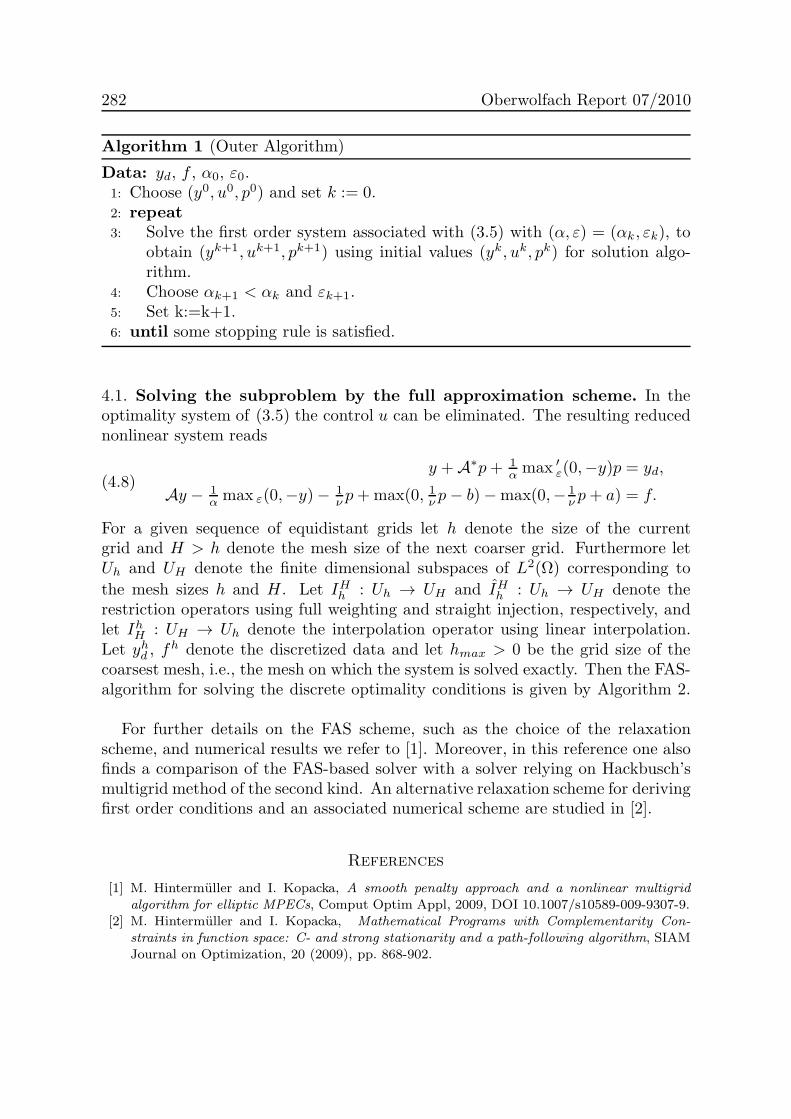
Algorithm 1 (Outer Algorithm)
Data: yd, f , α0, ε0.1: Choose (y0, u0, p0) and set k := 0.2: repeat3: Solve the first order system associated with (3.5) with (α, ε) = (αk, εk), to
obtain (yk+1, uk+1, pk+1) using initial values (yk, uk, pk) for solution algo-rithm.
4: Choose αk+1 < αk and εk+1.5: Set k:=k+1.6: until some stopping rule is satisfied.
4.1. Solving the subproblem by the full approximation scheme. In theoptimality system of (3.5) the control u can be eliminated. The resulting reducednonlinear system reads
(4.8)y +A∗p+ 1
α max ′ε(0,−y)p = yd,
Ay − 1α max ε(0,−y)− 1
ν p+max(0, 1ν p− b)−max(0,− 1ν p+ a) = f.
For a given sequence of equidistant grids let h denote the size of the currentgrid and H > h denote the mesh size of the next coarser grid. Furthermore letUh and UH denote the finite dimensional subspaces of L2(Ω) corresponding to
the mesh sizes h and H . Let IHh : Uh → UH and IHh : Uh → UH denote therestriction operators using full weighting and straight injection, respectively, andlet IhH : UH → Uh denote the interpolation operator using linear interpolation.Let yhd , f
h denote the discretized data and let hmax > 0 be the grid size of thecoarsest mesh, i.e., the mesh on which the system is solved exactly. Then the FAS-algorithm for solving the discrete optimality conditions is given by Algorithm 2.
For further details on the FAS scheme, such as the choice of the relaxationscheme, and numerical results we refer to [1]. Moreover, in this reference one alsofinds a comparison of the FAS-based solver with a solver relying on Hackbusch’smultigrid method of the second kind. An alternative relaxation scheme for derivingfirst order conditions and an associated numerical scheme are studied in [2].
References
[1] M. Hintermuller and I. Kopacka, A smooth penalty approach and a nonlinear multigridalgorithm for elliptic MPECs, Comput Optim Appl, 2009, DOI 10.1007/s10589-009-9307-9.
[2] M. Hintermuller and I. Kopacka, Mathematical Programs with Complementarity Con-straints in function space: C- and strong stationarity and a path-following algorithm, SIAMJournal on Optimization, 20 (2009), pp. 868-902.

Simulation, Control and Analysis for Interfaces and Free Boundaries 283
Algorithm 2 (FAS-algorithm)
Data: (yhd , fh), initial values (yh, ph).
1: if h = hmax then2: solve (4.8) exactly.3: else4: Do νpre pre-smoothing steps.5: Compute residuals rha = yhd − yh − (Ah)∗ph − 1
α max ′ε(0,−yh)ph and rhs =
fh −Ahyh + 1α max ε(0,−yh)− 1
ν ph.
6: Restrict residuals to coarser grid using full weighting rHa = IHh rha , r
Hs =
IHh rhs .
7: Restrict (yh, ph) to coarser grid using straight injection yH = IHh yh, pH =
IHh ph.
8: Compute right hand sides for coarse problem yHd = rHa + yH + (AH)∗pH +1α max ε
′(0,−yH)pH , fH = rHs +AHyH − 1α max ε(0,−yH)− 1
ν pH .
9: Apply γ-times the FAS-algorithm to coarse grid problem with h = H , righthand side (yHd , f
H) and initial values (yH , pH) to compute new approxima-tion (yH , pH).
10: Coarse grid correction: yh = yh + IhH(yH − yH), ph = ph + IhH(pH − pH),where IhH denotes the interpolation operator using linear interpolation.
11: Do νpost post-smoothing steps.12: end if
Motion of phase boundaries by geometric evolution equations
Yoshihito Kohsaka
(joint work with Harald Garcke, Kazuo Ito)
The surface diffusion equation
V = −∆ΓH
is a geometric evolution equation for an evolving hypersurface Γ = Γtt≥0. Here,V is the normal velocity of the surface, H is the mean curvature of the surface, and∆Γ is the Laplace-Beltrami operator of the surface. This equation was introducedby Mullins [2] to model the motion of interfaces in the case that the motion ofinterfaces is governed purely by mass diffusion within the interfaces (for simplicitywe set the diffusion constant to 1). Also, the surface diffusion equation is derivedas the H−1-gradient flow of the area functional for the surface (see [3]), so that anevolving hypersurface Γ has the property that the perimeter of the enclosed volumedecreases whereas the volume is conserved. On the other hand, when viewing thesurface diffusion equation as a partial differential equation (PDE), this equationis a fourth order nonlinear parabolic PDE. Thus, the maximum principle, whichis a useful tool of analyzing second order parabolic PDEs, does not work.
In this paper we study the motion of three curves Γit (i = 1, 2, 3) by surfacediffusion. These three curves are contained in a bounded domain Ω ⊂ R2 with

284 Oberwolfach Report 07/2010
the conditions that each one of the end points of Γit (i = 1, 2, 3) is connected ata triple junction p(t) ∈ Ω and the other end points intersect with ∂Ω. Then themotion of Γit (i = 1, 2, 3) are governed by
V i = −mi(γiκi)ss on Γit
with the boundary conditions at a triple junction p(t)
(1)
∠(Γ1t ,Γ
2t ) = θ3, ∠(Γ2
t ,Γ3t ) = θ1, ∠(Γ3
t ,Γ1t ) = θ2,
γ1κ1 + γ2κ2 + γ3κ3 = 0,
m1(γ1κ1)s = m2(γ2κ2)s = m3(γ3κ3)s,
and at Γit ∩ ∂Ω(2) Γit⊥∂Ω, (γiκi)s = 0.
Here, V i is the normal velocity of Γit, κi is the curvature of Γit, and s is an arc-
length parameter of Γit. Further, mi and γi are positive constants concerning the
mobility and the surface energy, respectively. In addition, θi are positive constantssatisfying
sin θ1
γ1=
sin θ2
γ2=
sin θ3
γ3,
which is called Young’s law. The boundary conditions (1) and (2) are the naturalboundary conditions when viewing the flow as the H−1-gradient flow of the energyfunctional
E[Γt] :=
3∑
i=1
γiL[Γit],
where Γt =⋃3i=1 Γ
it and L[Γ
it] is the length functional of Γit. Indeed, set
M(Γ) :=(u1, u2, u3) ∈ H
1(Γ)∣∣u1 + u2 + u3 = 0 at triple junction,∫
Γ1
u1 ds =
∫
Γ2
u2 ds =
∫
Γ3
u3 ds
with H1(Γ) := H1(Γ1) × H1(Γ2) × H1(Γ3). Then the H−1-inner product corre-sponding to this system is given by
(v1,v2)−1 :=3∑
i=1
mi
∫
Γi
∂suiv1∂su
iv2ds,
where uvj= (u1
vj, u2
vj, u3
vj) ∈ M(Γ) (j = 1, 2) is a weak solution of
(3)
−mi∂2suiv= vi on Γi (i = 1, 2, 3),
u1v+ u2
v+ u3
v= 0 at triple junction,
m1∂su1v= m2∂su
2v= m3∂u3
vat triple junction,
∂suiv= 0 at Γi ∩ ∂Ω (i = 1, 2, 3)
Simulation, Control and Analysis for Interfaces and Free Boundaries 285
for vj = (v1j , v2j , v
3j ) ∈ X(Γ) :=
(v1, v2, v3) ∈ (H1)′(Γ) | 〈v1, 1〉 = 〈v2, 1〉 = 〈v3, 1〉
.
Here 〈·, ·〉 is the duality pairing between (H1(Γi))′ and H1(Γi). Since a Poincare-type inequality holds for u ∈ M(Γ), we can prove that (3) has a unique weaksolution for v ∈ X(Γ).
Our goal here is to obtain a linearized stability criterion of stationary curves. To
mention it, we introduce some notation. Let Γ∗ =⋃3i=1 Γ
i∗ be stationary curves.
That is, Γi∗ is a part of circle or a line segment. Then we denote by ℓi∗ the lengthof Γi∗, by κ
i∗ the curvature of Γi∗, and by hi∗ the curvature of ∂Ω at Γi∗ ∩ ∂Ω. Now
we are ready to state our results. Since space is lacking to explain fully, we showonly one case. With regard to the other cases and details, see [1].
Theorem. Let γ1 = γ2 = γ3 = 1, κ1∗ = 0, κ2∗ = −κ3∗ = −1/2, ℓ1∗ =√3, and
ℓ3∗ = 4π/3. Also, set
Λ(h1∗, h2∗, h
3∗) := a123h
1∗h
2∗h
3∗+a12h
1∗h
2∗+a23h
2∗h
3∗+a31h
3∗h
1∗+a1h
1∗+a2h
2∗+a3h
3∗+a0,
where a123, a12, · · · , a0 are constants depending continuously on ℓ2∗ and satisfying
4(ajak − ajka0)(akiaij − a123ai)− (akiaj + aijak − a123a0 − ajkai)2 = 0,
akiaij − a123ai ≥ 0
for (i, j, k) = (1, 2, 3), (2, 3, 1), (3, 1, 2) and 0 < ℓ2∗ < 8π/3. Further, let NU be thenumber of positive eigenvalues for the linearized operator around Γ∗, and set
R1 := (h1∗, h2∗, h3∗) ∈ R+ |hi∗ > hi∗,a (i = 1, 2, 3), R3 := R+ \R1,
R4 := (h1∗, h2∗, h3∗) ∈ R− |hi∗ < hi∗,a (i = 1, 2, 3), R2 := R− \R4,
whereR+ := (h1∗, h2∗, h3∗) |Λ(h1∗, h2∗, h3∗) > 0,R− := (h1∗, h2∗, h3∗) |Λ(h1∗, h2∗, h3∗) <0, and hi∗,a := −ajk/a123 for (i, j, k) = (1, 2, 3), (2, 3, 1), (3, 1, 2). Then we obtain
(i) NU = 0 if (h1∗, h2∗, h
3∗) ∈ R1, (ii) NU = 1 if (h1∗, h
2∗, h
3∗) ∈ R2,
(iii) NU = 2 if (h1∗, h2∗, h
3∗) ∈ R3, (iv) NU = 3 if (h1∗, h
2∗, h
3∗) ∈ R4.
That is, in the case (i), Γ∗ is linearly stable.
Remark. When (h1∗, h2∗, h
3∗) is included in S := (h1∗, h2∗, h3∗) |Λ(h1∗, h2∗, h3∗) = 0,
zero eigenvalues of the linearized operator appear and their multiplicity is oneexcept in the case (h1∗, h
2∗, h
3∗) = (h1∗,c, h
2∗,c, h
3∗,c), where
hi∗,c := −akiaj + aijak − a123a0 − ajkai2(akiajk − a123ai)
for (i, j, k) = (1, 2, 3), (2, 3, 1), (3, 1, 2). At (h1∗,c, h2∗,c, h
3∗,c) the multiplicity of zero
eigenvalue is two. Also, taking account of the sign of hi∗,a − hi∗,c (i = 1, 2, 3), weobtain that the configuration of S is classified into two type (see Figure 1 & 2).

286 Oberwolfach Report 07/2010
-0.3
-0.2
-0.1
0
0.1
0.2
0.3
0.2 0.4 0.6 0.8 1 1.2 1.4
l2h1;a h1; -10
-8
-6
-4
-2
0
2
4
6
8
10
0.2 0.4 0.6 0.8 1 1.2 1.4
l2h2;a h2; -0.15
-0.1
-0.05
0
0.05
0.2 0.4 0.6 0.8 1 1.2 1.4l2
h3;a h3; Figure 1 :The graphs of hi
∗,a − hi∗,c for the parameter ℓ2.
R1R2R3R4
S1S2S3
-4 -3 -2 -1 0 1 2h1
-2
0
h2
-1
-0.8
-0.6
-0.4
-0.2
0
h3
hi;a > hi; (i = 1; 2; 3)
R1R2R3R4
S1S2S3
-4 -3 -2 -1 0 1h1
-2
0
2
h2
-1.5
-1
-0.5
0
0.5
h3
hi;a < hi; (i = 1; 2; 3)Figure 2 : The configuration of S (= S1 ∪S2 ∪S3).
References
[1] H. Garcke, K. Ito, and Y. Kohsaka, Surface diffusion with triple junctions: A stabilitycriterion for stationary solutions, to appear in Advances in Differential Equations.
[2] W. W. Mullins, Theory of thermal grooving, J. Appl. Phys., 28 (1957), 333–339.[3] J. E. Taylor and J. W. Cahn, Linking anisotropic sharp and diffuse surface motion laws via
gradient flows, J. Stat. Phys. 77, no.1-2 (1994), 183–197.
Nonsmooth Schur Newton Methods for Nonsmooth Saddle PointProblems
Ralf Kornhuber
(joint work with Carsten Graser, Uli Sack)
The numerical simulation of the coarsening of binary alloys based on the Cahn-Larche equations requires fast, reliable and robust solvers for Cahn-Hilliard equa-tions with logarithmic potential. After semi-implicit time discretization as intro-duced by Blowey and Elliott 92, the resulting spatial problem can be reformulatedas a non-smooth pde-constrained optimal control problem with cost functional in-duced by the Laplacian. The associated Karush-Kuhn-Tucker conditions take theform of a nonsmooth saddle point problem degenerating to a variational inclusionin the deep quench limit.

Simulation, Control and Analysis for Interfaces and Free Boundaries 287
Our considerations are based on recent work of Graser & Kornhuber 09 and theupcoming dissertation of Graser 10. The starting point is the elimination of theprimal variable leading to a nonlinear Schur complement which turns out to be theFrchet derivative of a convex functional. Now so-called nonsmooth Schur-Newtonmethods can be derived as gradient-related descent methods applied to this func-tional. In the discrete case we can show global convergence for an exact andan inexact version independent of any regularization parameters. Local quadraticconvergence or finite termination can be shown for piecewise smooth nonlinearitiesor in the deep quench limit respectively. The algorithm can be reinterpreted as apreconditioned Uzawa method and generalizes the well-known primal-dual activeset strategy by Kunisch, Ito, and Hintermuller 03. A (discrete) Allen-Cahn-typeproblem and a linear saddle point problem have to be solved (approximately) ineach iteration step. In numerical computations we observe mesh-independent localconvergence for initial iterates provided by nested iteration. In the deep quenchlimit, the numerical complexity of the (approximate) solution of the arising linearsaddle point problem dominates the detection of the actual active set.
Recent related approaches to nonsmooth saddle point problems by Banas &Nurnberg 09, Blank, Butz & Garcke 09, and Hintermuller, Hinze & Tber 09 werealso discussed.
Self-similar rupture in thin films with slip
Barbara Niethammer
(joint work with A. Munch, D. Peschka)
We consider rupture of thin viscous films in the strong-slip regime with smallReynolds numbers in a model derived in [1]. Numerical simulations indicate self-similar behaviour near the rupture point. More precisely, they suggest that viscos-ity and van-der-Waals forces are dominant and that there are self-similar solutionsof the second kind [2], that is the scaling in the spatial variable is not a-prioridetermined by a balance of force terms in the equation. More precisely, the filmthickness h and the horizontal velocity u follow
h(t, y) ∼ (t∗ − t)αH(η) and u(t, y) ∼ (t∗ − t)β−1U(η) ,
where η = (y − y∗)/(t∗ − t)β and y∗, t∗ denote the point and time of rupturerespectively. The scaling exponent α is 1/3, while β is not determined by thebalance of the dominant terms.
Second-kind similarity solutions also appear in simple models for inertialessjet pinch-off. In [5] convergence to these solutions is discussed. Under strongassumptions on the evolution of the jet the authors show that the selection of theself-similar solution in this model is solely determined by the behaviour of theinitial data around their minimum. This behaviour is expected, but a rigorousanalysis without a priori assumptions on the solutions has still been elusive.
Our goal in [3] is to provide such an analysis for viscosity dominated thin-filmrupture that is also directly applicable to the model of jet pinch-off considered in

288 Oberwolfach Report 07/2010
[5]. For a simplified model, where only terms accounting for viscous and van-der-Waals forces are kept, we rigorously establish finite time rupture in [2] followingideas of Renardy [4, 5] for jet pinch-off. In [3] we rigorously study the self-similarnature of the rupture. We show that for each β > 0 there exists a unique self-similar solution and equivalently these self-similar solutions can be uniquely char-acterized by their behaviour H(η) = H0+Hρη
ρ as η → 0, where ρ = ρ(β) ∈ (0,∞).Next, we investigate whether solutions of the time-dependent problem converge toa self-similar shape and, in case they do, which self-similar solution, i.e. which ρ(or β), is selected. As expected, the long-time asymptotics are completely deter-mined by the behaviour of the initial profile h(0, y) at its minimum. We establisha necessary and sufficient condition for convergence to any of the self-similar so-lutions with 0 < ρ < 3/2. The precise criterion is that the solution converges ifand only if the data are regularly varying at their minimum with index ρ. Thecorresponding scaling is the one associated to the self-similar solution up to someslowly varying function given by the initial data. These results are very similar innature to the dynamics in mean-field models for domain coarsening and coagula-tion, where the long-time behaviour depends sensitively on the tail of the initialdistribution functions.
We can prove the analogous characterization of domains of attraction for everypositive ρ under an additional assumption, namely that an associated nonlocalfunctional converges sufficiently fast. Presently we have no proof whether thisassumption is satisfied for regularly varying data. Numerical results indicate thatit is, but they also show that the situation is much more involved than in the caseof 0 < ρ < 3/2 and the details of the convergence proof must be different.
References
[1] A. Munch, B. Wagner, and T.P. Witelski. Lubrication models with small to large slip lengths.Journal of Engineering Mathematics, 53:359–383, Dec 2005.
[2] D. Peschka, A. Munch and B. Niethammer. Thin film rupture for large slip. J. Eng. Math.,66(1-3):33-51 (2010).
[3] D. Peschka, A. Munch and B. Niethammer. Self-similar rupture of viscous thin films in thestrong slip regime. Nonlinearity, 23(2):409-427 (2010)
[4] M. Renardy. A comment on self-similar breakup for inertialess Newtonian liquid jets. IMAJ. Appl. Math., 70(3):353–358, 2005.
[5] M. Renardy. Finite time breakup of viscous filaments. Z. Angew. Math. Phys., 52(5):881–887,2001.
Parametric approximation of geometric evolution equations andapplications to the modelling of snowflake growth
Robert Nurnberg
(joint work with John W. Barrett, Harald Garcke)
Geometric evolution equations in general arise as gradient flows for a free energyfor a curve or surface. In applications these hypersurfaces often play the role of aninterface or a free boundary. In this talk, we review a variational formulation for

Simulation, Control and Analysis for Interfaces and Free Boundaries 289
such geometric evolution laws that leads to discretizations with very good meshproperties, and we indicate how these formulations can be extended to situationswhere the interface evolution is coupled to a bulk equation.
Given a parameterization ~x(ρ, t) : I × [0, T ] → R2, I := R/Z, of the family ofclosed curves Γ(t) ⊂ R2, we note that the L2- and H−1-gradient flow of length,i.e. the curvature flow and the surface diffusion flow, respectively, can be writtenas
(1) ~xt . ~ν =
κ
−κss, κ ~ν = ~xss ,
with κ the curvature of Γ and ~ν a unit normal. Note that the formulation (1)is independent of the tangential component, ~xt . ~xs, of the velocity ~xt. However,when (1) is discretized with the help of piecewise linear finite elements, then thecorresponding discrete tangential velocity is no longer arbitrary. In fact, the spa-tially discrete solutions are such that the polygonal curves Γh(t), where they arenot locally flat, are equidistributed at every time t > 0.
On introducing the appropriate spaces V h and V h of periodic piecewise lin-ear vector- and scalar-valued parametric finite elements, we obtain the followingsemidiscrete continuous-in-time approximation of (1). Given Γh(0), for t ∈ (0, T ]
find Γh(t) = ~Xh(I, t), with ~Xh(t) ∈ V h, and κh(t) ∈ V h such that
〈 ~Xht , χ ~ν
h〉hh −〈κh, χ〉hh〈κhs , χs〉h
= 0 ∀ χ ∈ V h,(2a)
〈κh ~νh, ~η〉hh + 〈 ~Xhs , ~ηs〉m = 0 ∀ ~η ∈ V h;(2b)
where 〈f, g〉h :=∫Γh(t)
f . g ds =∫If . g | ~Xh
ρ (t)| dρ with 〈·, ·〉hm the mass lumped in-
ner product. It is now straightforward to show that (2b) implies that neighbouring
elements of Γh(t) = ~Xh(I, t) have the same length or are parallel. When introduc-ing fully discrete approximations, it is possible to use semi-implicit time steppingor a fully implicit approach. In the former case, we obtain linear schemes that in-trinsically move mesh points tangentially so that e.g. numerical steady states arealways equidistributed, while the latter leads to highly nonlinear approximationsthat truly equistribute at each time level; see [1, 2] and [9], respectively. Bothvariants are unconditionally stable.
An advantage of our scheme (2a,b), that follows from the formulation (1), isthat other geometric evolution laws can be handled easily. For example, nonlinearcurvature flow, including the inverse curvature flow, area preserving curvatureflow, Willmore flow (or elastic flow) for curves, as well as higher codimension flowsof curves in Rd, d ≥ 3, and geodesic flows of curves flowing on a given manifold,can all be considered; see [1, 2, 10] for details.
The approximation (2a,b) can also be generalized to cover the geometric evolu-tion of curve networks, where different curves move by their given normal velocitiesand where certain conditions have to hold at triple junctions, where three curves

290 Oberwolfach Report 07/2010
meet at a point. It turns out that the natural generalization of the weak formula-tion used to derive (2a,b) approximates all the necessary triple junction conditionscorrectly; see [1, 2].
Replacing the isotropic curve length |Γ| :=∫Γ1 ds with a weighted length of
the form |Γ|γ :=∫Γγ(~ν) ds, where γ : R2 \~0 → R>0 is a given one-homogeneous
anisotropy function, yields the anisotropic analogues of the geometric evolutionequations of curvature flow and surface diffusion, i.e.
(3) ~xt . ~ν =
β(~ν)κγ
−(β(~ν) [κγ ]s)s, κγ ~ν = [γ′(~ν)]⊥s ,
where ~ν = −~x⊥s , κγ is the weighted curvature, and β : S1 → R>0 is an anisotropicmobility. The finite element approximations based on (2a,b) can now be extendedto approximate the flows (3). The fully discrete schemes can be shown to beunconditionally stable for arbitrary smooth convex anisotropies, in the case of afully implicit time discretization ([9]), and for anisotropies of the form
(4) γ(~p) =
[L∑
ℓ=1
[γ(ℓ)(~p)]r
] 1r
=
[L∑
ℓ=1
[~p .G(ℓ) ~p]r2
] 1r
,
whereG(ℓ) ∈ R2×2, ℓ = 1 → L, are symmetric and positive definite, and r ∈ [1,∞);see [3, 10].
Moreover, the ideas presented above naturally generalize to the approximationof geometric evolution equations for hypersurfaces in R3. Examples are the meancurvature flow, nonlinear mean curvature flow and surface diffusion for isotropic(see [4]) and anisotropic surface energies (see [6]), the Willmore flow and Helfrichflow (see [5]), as well as the evolution of surface clusters with triple junction linesand quadruple junction points (see [7]). In all of the isotropic cases, we can showthat our semidiscrete continuous-in-time approximations produce triangulationswith very good mesh qualities, so called conformal polyhedral surfaces; see [4, §4]for details. Such surfaces are characterized by the fact that the two popular notionsof discrete vertex normals, given by the directions of steepest descent of area andvolume, respectively, coincide; which in turn means that the triangulation cannotbe bad. Related properties can be derived for anisotropic surface energies.
Finally, we can also consider situations where the interface evolution is coupledto an equation that needs to hold in a bulk domain. For instance, the evolution ofa solidifying front Γ(t) in a Stefan problem with anisotropic Gibbs-Thomson lawand kinetic undercooling can be expressed as
(5) ρ (~xt . ~ν) = β(~ν) [ακγ − a u] on Γ(t),
where u, usually a rescaled temperature, satisfies a heat equation in the bulk do-main Ω, with an energy balance at the interface leading to jumps in the gradientof u across Γ(t). Coupling our natural parametric finite element approximation of(5) to a finite element approximation of the evolution of u in the bulk, we are ableto introduce stable fully discrete schemes which mimic the underlying Lyapunov

Simulation, Control and Analysis for Interfaces and Free Boundaries 291
Figure 1. Solid plates and sectored plates.
structure of the continuous problem, see [8]. When u is interpreted as a concentra-tion, then the studied Stefan problem can be used to model the solidification froma supersaturated solution, which is relevant for snowflake growth. An examplecomputation, for a surface energy of the form (4) with a hexagonal prism Wulffshape, can be seen in Figure 1.
References
[1] J.W. Barrett, H. Garcke, and R. Nurnberg, A parametric finite element method for fourthorder geometric evolution equations, J. Comput. Phys. 222 (2007), 441–462.
[2] J.W. Barrett, H. Garcke, and R. Nurnberg, On the variational approximation of combinedsecond and fourth order geometric evolution equations, SIAM J. Sci. Comput. 29 (2007),1006–1041.
[3] J.W. Barrett, H. Garcke, and R. Nurnberg, Numerical approximation of anisotropic geo-metric evolution equations in the plane, IMA J. Numer. Anal. 28 (2008), 292–330.
[4] J.W. Barrett, H. Garcke, and R. Nurnberg, On the parametric finite element approximationof evolving hypersurfaces in R3, J. Comput. Phys. 227 (2008), 4281–4307.
[5] J.W. Barrett, H. Garcke, and R. Nurnberg, Parametric approximation of Willmore flowand related geometric evolution equations, SIAM J. Sci. Comput. 31 (2008), 225–253.
[6] J.W. Barrett, H. Garcke, and R. Nurnberg, A variational formulation of anisotropic geo-metric evolution equations in higher dimensions, Numer. Math. 109 (2008), 1–44.
[7] J.W. Barrett, H. Garcke, and R. Nurnberg, Parametric approximation of surface clustersdriven by isotropic and anisotropic surface energies, 2009, Preprint No. 04/2009, UniversityRegensburg.
[8] J.W. Barrett, H. Garcke, and R. Nurnberg, On stable parametric finite element methods forthe Stefan problem and the Mullins–Sekerka problem with applications to dendritic growth,2009, Preprint No. 21/2009, University Regensburg.
[9] J.W. Barrett, H. Garcke, and R. Nurnberg, The approximation of planar curve evolutions bystable fully implicit finite element schemes that equidistribute, 2009, Preprint No. 29/2009,University Regensburg.
[10] J.W. Barrett, H. Garcke, and R. Nurnberg, Numerical approximation of gradient flows forclosed curves in Rd, IMA J. Numer. Anal. 30 (2010), 4–60.
Level set method for spiral crystal growth and surface evolution
Takeshi Ohtsuka
This is a brief introduction to a level set formulation for spiral patterns evolvingby a mean curvature flow with driving force, and numerical simulations for crystalgrowth with aid of screw dislocations, which is called spiral crystal growth (see [1]).When partial displacements in the lattice of atoms, that is called screw dislocation,across the surface of a crystal, then steps are provided on the surface. The steps
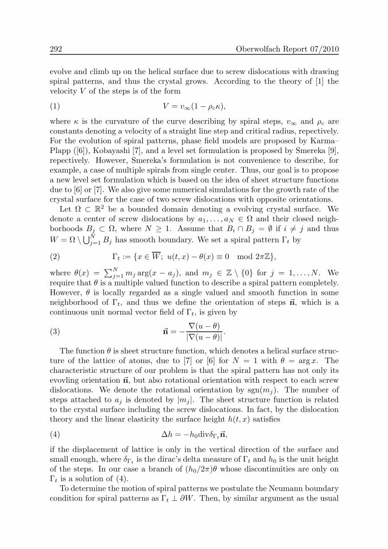
292 Oberwolfach Report 07/2010
evolve and climb up on the helical surface due to screw dislocations with drawingspiral patterns, and thus the crystal grows. According to the theory of [1] thevelocity V of the steps is of the form
(1) V = v∞(1− ρcκ),
where κ is the curvature of the curve describing by spiral steps, v∞ and ρc areconstants denoting a velocity of a straight line step and critical radius, repectively.For the evolution of spiral patterns, phase field models are proposed by Karma–Plapp ([6]), Kobayashi [7], and a level set formulation is proposed by Smereka [9],repectively. However, Smereka’s formulation is not convenience to describe, forexample, a case of multiple spirals from single center. Thus, our goal is to proposea new level set formulation which is based on the idea of sheet structure functionsdue to [6] or [7]. We also give some numerical simulations for the growth rate of thecrystal surface for the case of two screw dislocations with opposite orientations.
Let Ω ⊂ R2 be a bounded domain denoting a evolving crystal surface. Wedenote a center of screw dislocations by a1, . . . , aN ∈ Ω and their closed neigh-borhoods Bj ⊂ Ω, where N ≥ 1. Assume that Bi ∩ Bj = ∅ if i 6= j and thus
W = Ω \⋃Nj=1 Bj has smooth boundary. We set a spiral pattern Γt by
(2) Γt := x ∈W ; u(t, x)− θ(x) ≡ 0 mod 2πZ,
where θ(x) =∑N
j=1mj arg(x − aj), and mj ∈ Z \ 0 for j = 1, . . . , N . Werequire that θ is a multiple valued function to describe a spiral pattern completely.However, θ is locally regarded as a single valued and smooth function in someneighborhood of Γt, and thus we define the orientation of steps ~n, which is acontinuous unit normal vector field of Γt, is given by
(3) ~n = − ∇(u− θ)
|∇(u− θ)| .
The function θ is sheet structure function, which denotes a helical surface struc-ture of the lattice of atoms, due to [7] or [6] for N = 1 with θ = arg x. Thecharacteristic structure of our problem is that the spiral pattern has not only itsevovling orientation ~n, but also rotational orientation with respect to each screwdislocations. We denote the rotational orientation by sgn(mj). The number ofsteps attached to aj is denoted by |mj |. The sheet structure function is relatedto the crystal surface including the screw dislocations. In fact, by the dislocationtheory and the linear elasticity the surface height h(t, x) satisfies
(4) ∆h = −h0divδΓt~n,
if the displacement of lattice is only in the vertical direction of the surface andsmall enough, where δΓt
is the dirac’s delta measure of Γt and h0 is the unit heightof the steps. In our case a branch of (h0/2π)θ whose discontinuities are only onΓt is a solution of (4).
To determine the motion of spiral patterns we postulate the Neumann boundarycondition for spiral patterns as Γt ⊥ ∂W . Then, by similar argument as the usual

Simulation, Control and Analysis for Interfaces and Free Boundaries 293
level set method (see [5]) we obtain the level set equation as follows;
(5)
ut − v∞|∇(u− θ)|1 + ρcdiv
∇(u− θ)
|∇(u− θ)|
= 0 in (0, T )×W,
〈~ν,∇(u− θ)〉 = 0 on (0, T )× ∂W,
u|t=0 = u0 on W,
where ~ν is the outer unit normal vector field of ∂W , 〈·, ·〉 is the usual inner productin R2, and u0 is an initial datum satisfying
(6) Γ0 = x ∈ W ; u0(x)− θ(x) ≡ 0 mod 2πZ.We can define a viscosity solution to (5) in usual way (see [3]). The comparison,existence and uniqueness of viscosity solutions global-in-time for u0 ∈ C(W ) isobtained by [8]. However, it is not clear the existence of u0 ∈ C(W ) satisfying (6).Goto, Nakagawa and the author prove the existence of u0 ∈ C(W ) for suitableinitial pattern Γ0. Moreover, they prove the uniqueness of Γt obtained from ourlevel set formulation with respect to the initial pattern Γ0. The basic strategy ofthe proofs are based on the method as in [2] or [4].
It is convenience for understanding our formulation to introduce a coveringspace which is based on θ. Formally we now introduce
X := (x, z); z ≡ θ(x) mod 2πZ.Then we find that X is divided into three regions as follows;
Γt := (x, z) ∈ X ; u(t, x)− z = 0,It := (x, z) ∈ X ; u(t, x)− z > 0,Ot := (x, z) ∈ X ; u(t, x)− z < 0.
We observe that Γt is the image of Γt by the projection (x, z) 7→ x, and also (3)
is determined from It and Ot; we consider steps evolve from It’s side to Ot’s side.The covering space is very convenient to remove the difficulties which come fromthe multiplicity of θ, that is the crucial difficulty of our problem. In particular, the
uniqueness of Γt is obtained from the comparison of It and Ot between viscositysub- and supersolution.
The covering space X is also useful to obtain the surface height h(t, x). Once
we obtain a solution u to (5), we set h : [0,∞)×X → R as
ζ(t, x, z) = z − 2πk if (x, z) ∈ (y, η) ∈ X ; u(t, x)− z ∈ [2πk, 2π(k + 1)).
Let Θj(x) ∈ [0, 2π) is the principal value of arg(x−aj) and Θ(x) =∑Nj=1mjΘj(x).
We set
ζ(t, x) = ζ(t, x,Θ(x)).
Then, we observe that ζ ≡ θ mod 2πZ and the discontinuities of ζ lie only on Γt.
Moreover, we obtain that It = (x, z) ∈ X ; ζ(t, x) + π− z > 0. Consequently, we
294 Oberwolfach Report 07/2010
set the height function h as
h(t, x) =h02π
(ζ(t, x) + π).
The growth height of the surface is calculated as
Rh(t; t0) =1
|W |
∫
W
[h(t, x)− h(t0, x)]dx.
The growth rate of the surface is calculated as R′h(t; t0) if Rh is smooth.
In this talk we propose a numerical results of the growth height in the caseN = 2, m1 = −m2 = 1, and W = Ω \ (Bρ(a1) ∪ Bρ(a2)), where Bρ(a) is theclosed disc whose center and radius is a and ρ, repectively. In [1] it is pointedout that the pair whose rotational orientations are opposite have no activity if|a1 − a2| < 2ρc. We call such a pair inactive pair. The existence of inactive pairsare not only verified numerically but also proved mathemtaically.
Theorem. Let Ω be a bounded domain such that B4ρc(0) ⊂ Ω. Let W =Ω \ (Bρ(a1) ∪Bρ(a2)), θ(x) = arg(x− a1)− arg(x − a2), a1 = (−r, 0), a2 = (r, 0)with r ∈ (0, ρc), and ρ ∈ (0, ρc). Then, for any viscosity solution u to (5), thereexists M > 0 such that u(t, x) < M for t > 0 and x ∈W .
The idea of the proof is to construct a stationary solution to (5) by θ. We knowthat C(b) := x ∈ R2; |x− b| = ρc for b ∈ R2 is a stationary solution of (1), andthere exist b ∈ R2 and a part of C(b) satisfying ∂W ⊥ C(b) if |a1 − a2| < 2ρc.Then, we obtain that θC(b), that is one of branches of θ whose discontinuities areonly on C(b), is a viscosity solution of (5) by direct calculation.
References
[1] W. K. Burton, N. Cabrera and F. C. Frank, The growth of crystals and the equilibriumstructure of their surfaces, Philos. Trans. Roy. Soc. London. Ser. A. 243(1951), 299–358.
[2] Y.-G. Chen, Y. Giga and S. Goto, Uniqueness and existence of viscosity solutions of gener-alized mean curvature flow equation, J. Differential Geom. 33(1991), 749–786.
[3] M. Crandall, H. Ishii and P.-L. Lions, User’s guide to viscosity solutions of second orderpartial differential equations, Bull. Amer. Math. Soc. 27(1992), 1–67.
[4] L. C. Evans and J. Spruck, Motion of level sets by mean curvature I, J. Differential Geom.33(1991), 635–681.
[5] Y. Giga, Surface evolution equation –A level set approach, Birkhauser, 2006.[6] A. Karma and M. Plapp, Spiral surface growth without desorption, Physical Review Letters
81(1998), 4444–4447.[7] R. Kobayashi, private communication.[8] T. Ohtsuka, A level set method for spiral crystal growth, Adv. Math. Sci. Appl. 13(2003),
225–248.[9] P. Smereka, Spiral crystal growth, Physica D, 138(2000), 282–301.

Simulation, Control and Analysis for Interfaces and Free Boundaries 295
FEM approximation of the anisotropic mean curvature flow in highercodimension
P. Pozzi
Anisotropic mean curvature flow has been widely studied, both analytically andnumerically. Much of the research concentrated so far on the case of codimensionequal to one, i.e. on the flow for hypersurfaces. In this talk we present recentprogress for the case of higher codimension.
After discussing the concept of anisotropic area functional, we consider theanisotropic mean curvature flow for parametric curves and two dimensional sur-faces in Rn for arbitraty n ≥ 3 and study its numerical approximation by finiteelements.
Stabilization of a fluid – structure model
Jean-Pierre Raymond
We study a system coupling the incompressible Navier-Stokes equations in 2Dbounded domains with a damped Euler-Bernoulli beam equation, where the beamis a part of the upper boundary of the domain occupied by the fluid. We also studysimilar systems in 3D domains, in that case the structure equation is a dampedplate equation. Due to the deformation of the beam (or the plate in 3D) the fluiddomain at time t depends on t. We are interested in exponential stabilization ofsuch systems, locally about a stationary solution, by controls acting either in thefluid equation or in the beam equation.
These results are obtained by studying stabilizability results for linearized sys-tems. In order to derive linearized systems, we first rewrite the nonlinear modelsin a cylindrical domain Ω × (0,∞), by using a change of variable defined thanksto the deformation of the structure. In the 2D case, the model linearized aboutthe null solution reads as follows
(1)
vt − div σ(v, p) = fχO, div v = 0 in Q∞,
v = η2~e2 on Σs∞, v = 0 on Σ0∞, v(0) = v0 in Ω,
η1,t = η2, η2,t − βη1,xx − δη2,xx + αMsη1,xxxx =Ms(ρ1p+ g) on Σs∞,
η1 = 0 and η1,x = 0 on0, L
× (0,∞),
η1(0) = η01 and η2(0) = η02 in Γs,
where Q∞ = Ω× (0,∞), Ω is a simply connected bounded domain with boundaryΓ, for simplicity we assume that Ω ⊂ (x, y) | y < 1, Γs = (0, L)×1 is a flat partof the boundary Γ, ~e2 = (0, 1)T , Σs∞ = Γs×(0,∞), Σ0
∞ = Γ0×(0,∞), Γ0 = Γ\Γs,Ms is the orthogonal projection in L2(Γs) onto L
20(Γs) = η ∈ L2(Γs) |
∫Γsη = 0,
σ(v, p) = ν(∇v+∇vT )− p I, ν > 0 is the fluid viscosity, α > 0, β ≥ 0, and δ > 0are the adimensional rigidity, stretching, and friction coefficients of the beam, ρ1 isa positive constant related to the densities of the fluid and of the structure, f is acontrol acting in the fluid equation, χO is the characteristic function of an open set

296 Oberwolfach Report 07/2010
O ⊂ Ω, g is a control acting in the beam equation. To simplify the presentation,we assume that either Ω is of class C2 or Ω is the rectangle (0, L)× (0, 1).
Let us introduce the spaces
L20(Ω) =
p ∈ L2(Ω) |
∫Ωp = 0
, Hσ(Ω) = Hσ(Ω) ∩ L2
0(Ω) for σ ≥ 0,
V0n(Ω) =
v ∈ L2(Ω;R2) | div v = 0, v · n = 0 on Γ
,
V0(Ω) =v ∈ L2(Ω;R2) | div v = 0
and V2
n(Ω) = H2(Ω;R2) ∩V0n(Ω).
We introduce the Leray projector P : L2(Ω;R2) 7→ V0n(Ω) and the Stokes operator
A0 = νP ∆ with domain D(A0) = H2(Ω;R2) ∩ H10 (Ω;R
2) ∩ V0n(Ω). We want
to study system (1) when v0 ∈ V0(Ω), η01 ∈ H20 (Γs) ∩ L2
0(Γs), η02 ∈ L2
0(Γs),g ∈ L2(0,∞;L2(Γs)), f ∈ L2(0,∞;L2(Ω;R2)), and when the initial data satisfythe compatibility condition
(2) v0 · n = η02 χΓs.
For that, we have to study the semigroup corresponding to system (1). We denoteby N ∈ L(H−1/2(Γ),H1(Ω)) the Neumann operator defined by N(g) = q, whereq is the solution of
∆q = 0 in Ω,∂q
∂n= g on Γ
(n is the unit normal to Γ outward Ω), and by D ∈ L(H−1/2(Γ;R2),V0(Ω)) theDirichlet operator defined by D(g) = w, where w is the solution of
−ν∆w +∇π = 0, divw = 0 in Ω, w = g on Γ.
We also need Ns(g) = N (g χΓs) and γs(q) = Ms(q|Γs
) (χΓsis the characteristic
function of Γs). When f = 0 and g = 0, we may rewrite system (1) in the form
(3)
Pvt = A0Pv + (−A0)PD(η2~e2 χΓs), v(0) = v0 in Ω,
(I − P )v = (I − P )D(η2~e2 χΓs),
η1,t = η2,
(I + γsNs)η2,t − βη1,xx − δη2,xx + αMsη1,xxxx = γsN(∆Pv · n) on Σs∞,
η1 = 0 and η1,x = 0 on0, L
× (0,∞),
η1(0) = η01 and η2(0) = η02 in Γs.
System (3) is of the form
d
dt
Pv
η1
η2
= A
Pv
η1
η2
, (I − P )v = (I − P )D(η2~e2 χΓs
),
Simulation, Control and Analysis for Interfaces and Free Boundaries 297
with
A =
I 0 0
0 I 0
0 0 (I + γsNs)−1
A0 0 (−A0)PD
0 0 I
γsN(∆(·) · n) Aα,β δ∆s
,
D(Aα,β) = H4(Γs) ∩H20 (Γs) ∩ L2
0(Γs), Aα,βη = βηxx − αηxxxx, ∆sη = ηxx,
and
D(A) =(Pv, η1, η2) ∈ V2
n(Ω)× (H4 ∩H20 ∩ L2
0)(Γs)× (H20 ∩ L2
0)(Γs)
| P (v −D(η2~e2 χΓs)) ∈ H1
0 (Ω;R2).
Theorem 1. The operator (A,D(A)) is the infinitesimal generator of an analyticsemigroup on H = V0
n(Ω) × (H20 (Γs) ∩ L2
0(Γs)) × L20(Γs), and the resolvent of A
is compact.This type of result can be extended to the 3D case.
Theorem 2. (Exponential stabilization with an internal control acting in the fluidequation) Assume that Ω is of class C2 and that g = 0. Then, for all ω > 0, thereexists a positive constant Cω such that, for all v0 ∈ V0(Ω), η01 ∈ H2
0 (Γs)∩L20(Γs),
η02 ∈ L20(Γs) satisfying (2), there exists a control f ∈ L2(0,∞;L2(Ω;R2)) for which
the solution of system (1) obeys
(4)‖(v(t), η1(t), η2(t))‖V0(Ω)×H2
0 (Γs)×L20(Γs)
≤ Cωe−ωt‖(v0, η01 , η
02)‖V0(Ω)×H2
0 (Γs)×L20(Γs).
The proof of Theorem 2 relies on Theorem 1 and on a unique continuation resultproved in [1]. This type of result can be extended to the 3D case.
Theorem 3. (Exponential stabilization with a control acting in the structureequation) Assume that Ω = (0, L)×(0, 1) and that f = 0. Then, for all ω > 0, thereexists a positive constant Cω such that, for all v0 ∈ V0(Ω), η01 ∈ H2
0 (Γs)∩L20(Γs),
η02 ∈ L20(Γs) satisfying (2), there exists a control g ∈ L2(0,∞;L2(Γs)) for which
the solution of system (1) obeys (4).The proof of Theorem 3 relies on Theorem 1 and on a unique continuation
result proved in [2]. This type of result can be extended to other domains in the2D case by using unique continuation results proved in [3], but there is no similarresult proved in the 3D case.
Thanks to Theorem 3, we can prove that the nonlinear system coupling theNavier-Stokes equations with the damped beam equation is exponentially stabiliz-able, locally about the null solution, with any prescribed decay rate, by a feedbackcontrol corresponding to a force term in the beam equation [4]. The feedback isapplied on the whole structure and it is determined, via a Riccati equation, bysolving an infinite time horizon control problem for the linearized model.
Thanks to Theorem 2, we can prove that the nonlinear system coupling theNavier-Stokes equations with the damped beam equation is exponentially stabiliz-able, locally about the null solution, with any prescribed decay rate, by a feedback
298 Oberwolfach Report 07/2010
control corresponding to a force term in the fluid equation. We think that similarresults could be obtained in the 3D case, but this is not yet done.
References
[1] C. Fabre, G. Lebeau, Regularite et unicite pour le probleme de Stokes, Comm. PartialDifferential Equations 27 (2002), 437–475.
[2] A. Osses, J.-P. Puel, Approximate controllability for a hydro-elastic model in a rectangulardomain, ISNM 133 (1999), 231-243.
[3] A. Osses, J.-P. Puel, Unique continuation property near a corner and its fluid-structure con-trollability consequences, ESAIM Control, Optimization and Calculus of Variations, DOI:10.1051/cocv:2008024.
[4] J.-P. Raymond, Feedback stabilization of a fluid - structure model, 2009, submitted to SIAMJ. Control and Optim..
Numerical methods for surfactant transport in two-phaseincompressible flows
Arnold Reusken
(joint work with P. Esser, J. Grande, S. Groß, M. Olshanskii)
1. A model for two-phase incompressible flows
We consider a two-phase flow problem with mass transport between the phasesand transport of a surfactant (“surface active agent”) on the interface between thephases. We briefly introduce a (standard) model for this type of flow problem.
Fluid dynamics. The domain Ω ⊂ Rd, d = 2 or d = 3, contains two differentimmiscible incompressible phases (fluid-fluid or fluid-gas) which may move in timeand have different material properties ρi (density) and µi (viscosity), i = 1, 2. Foreach point in time, t ∈ [0, T ], Ω is partitioned into two open bounded subdomainsΩ1(t) and Ω2(t), Ω = Ω1(t) ∪ Ω2(t), Ω1(t) ∩ Ω2(t) = ∅, each of them containingone of the phases. These phases are separated from each other by the interfaceΓ(t) = Ω1(t) ∩ Ω2(t). We assume isothermal conditions and that both phases arepure substances. Furthermore, we do not consider reaction or phase transition. Weintroduce the normal velocity VΓ = VΓ(x, t) ∈ R which denotes the magnitude ofthe velocity of the interface Γ at x ∈ Γ(t) in normal direction. The immiscibilityassumption is modeled by the condition VΓ = u · nΓ at the interface, with nΓ
the unit normal on Γ pointing from Ω1 to Ω2. We consider the following standardmodel (in strong formulation) for the fluid dynamics of a two-phase incompressible

Simulation, Control and Analysis for Interfaces and Free Boundaries 299
flow:ρi(
∂u
∂t+ (u · ∇)u) = divσi + ρig
divu = 0in Ωi, i = 1, 2,(1)
[σnΓ] = −τκnΓ −∇Γτ on Γ,(2)
[u] = 0 on Γ,(3)
VΓ = u · nΓ on Γ.(4)
with the stress tensor σi = −pI+ µi(∇u+ (∇u)T
). The density and viscosity, ρi
and µi, i = 1, 2, are assumed to be constant in each phase. The operator ∇Γ isthe tangential gradient. The parameter τ is the surface tension coefficient and κis the mean curvature of Γ, i.e., κ(x) = divnΓ(x) for x ∈ Γ. To make the problemwell-posed one needs suitable initial and boundary conditions for u.
Mass transport. We assume that one or both phases contain a dissolved species thatis transported due to convection and diffusion and does not adhere to the interface.The concentration of this species is denoted by c(x, t). This flow problem can bemodeled by the equations (1)-(4) for the flow variables and a convection-diffusionequation for the concentration c. At the interface we need interface conditions forc. The first interface condition comes from mass conservation, which implies fluxcontinuity. The second condition results from a constitutive equation known asHenry’s law. The model is as follows:
∂c
∂t+ u · ∇c = div(Di∇c) in Ωi, i = 1, 2,(5)
[Di∇c · nΓ] = 0 on Γ,
c1 = CHc2 on Γ.
The diffusion coefficient Di is assumed to be piecewise constant. In the interfacecondition we use the notation ci for c|Ωi
restricted to the interface. The constantCH > 0 is given (Henry’s constant). In general CH 6= 1, i.e. we have a disconti-nuity in c across Γ.
Surfactant transport. We assume that there is a species (called tenside or sur-factant) which adheres to the interface and is transported on the interface due toconvection (movement of the interface) and due to diffusion (molecular diffusion onthe interface). For simplicity we assume that there are no adsorption and desorp-tion effects. The concentration of this surfactant is denoted by S(x, t), x ∈ Γ(t). Apartial differential equation for this quantity can be derived from the conservationof mass principle. This results in the convection-diffusion problem
(6) S + S divΓu = divΓ(DΓ∇ΓS) on Γ.
Here S denotes the material derivative and divΓ is the tangential divergence op-erator.

300 Oberwolfach Report 07/2010
In the talk we presented an overview of numerical methods for treating the cou-pled model (1)-(6). Key ingredients are a level set method for interface capturing,finite element discretizations on a nested locally refined hierarchy of tetrahedralgrids and problem adapted preconditioners. A detailed overview is given in [3]. Anew finite element method for discretization of the surfactant transport equation(6) has been developed. The main idea is presented in section 2.
2. A new finite element method for the surfactant transportproblem
We outline the main idea of a new Eulerian finite element method for dis-cretization of the surfactant equation introduced in [1], for a simplified prob-lem, namely the Laplace-Beltrami problem. In weak formulation this problemis as follows: For given f ∈ L2
0(Γ) := v ∈ L2(Γ) |∫Γv ds = 0, determine
u ∈ H1∗ (Γ) := v ∈ H1(Γ) |
∫Γ v ds = 0 such that
(7)
∫
Γ
∇Γu · ∇Γv ds =
∫
Γ
fv ds for all v ∈ H1∗ (Γ).
We assume a stationary surface Γ and an approximation Γh of Γ. We assume thatthis approximate surface is constructed as follows. Let Thh>0 be a family oftetrahedral triangulations of a fixed domain Ω ⊂ R3 that contains Γ. These tri-angulations are assumed to be regular, consistent and stable. Take Th ∈ Thh>0.We assume that Γh is a C0,1 surface without boundary and Γh can be partitionedin planar segments, triangles or quadrilaterals, consistent with the outer triangu-lation Th. For any tetrahedron ST ∈ Th such that meas2(ST ∩ Γh) > 0 defineT = ST ∩ Γh. We assume that each T is planar, i.e., either a triangle or a quadri-lateral. Let Fh be the set of all triangles or quadrilaterals T such that T = ST ∩Γhis nonempty for some tetrahedron ST ∈ Th and Γh = ∪T∈Fh
T .The main new idea of the method is that for discretization of the problem (7) we
use a finite element space induced by the continuous linear finite elements on Th.This is done as follows. We define a subdomain that contains Γh: ωh := ∪T∈Fh
ST .This subdomain in R3 is connected and partitioned in tetrahedra that form a subsetof Th. We introduce the finite element space
Vh := vh ∈ C(ωh) | v|ST∈ P1 for all T ∈ Fh .
This space induces the following space on Γh:
(8) V Γh := ψh ∈ H1(Γh) | ∃ vh ∈ Vh : ψh = vh|Γh
,which is used for a Galerkin discretization of (7): determine uh ∈ V Γ
h with∫Γhuh ds = 0 such that
(9)
∫
Γh
∇Γhuh∇Γh
ψh ds =
∫
Γh
fhψh ds for all ψh ∈ V Γh ,
with fh a suitable extension of f such that∫Γhfh ds = 0. Due the Lax-Milgram
lemma this problem has a unique solution uh. The paper [1] presents a discretiza-tion error analysis of this method that shows that under reasonable assumptions

Simulation, Control and Analysis for Interfaces and Free Boundaries 301
we have optimal error bounds. In the talk we present these error bounds. Results ofnumerical experiments confirm the theoretical analysis. We remark that the familyThh>0 is shape-regular but the family Fhh>0 in general is not shape-regular.In practice Fh contains a significant number of strongly deteriorated triangles thathave very small angles. Moreover, neighboring triangles can have very differentareas.
We briefly address the issue of conditioning of the mass and stiffness, inves-tigated in [2]. Numerical experiments in two- and three-dimensional examplesindicate that in the 3D case both for the diagonally scaled mass and stiffness ma-trix (effective) spectral condition numbers behave as O(h−2) and in the 2D casethe behaviour of these condition numbers is O(h−3) and O(h−2), respectively.
References
[1] M.A. Olshanskii, A. Reusken, J. Grande, A Finite Element method for elliptic equations onsurfaces, SIAM J. Numer. Anal. 47 (2009), 3339–3358.
[2] M.A. Olshanskii, A. Reusken, A finite element method for surface PDEs: Matrix properties,Numerische Mathematik 114 (2010), 491–520.
[3] DROPS package for simulation of two-phase flows. //www.igpm.rwth-aachen.de/DROPS.
The Allen–Cahn action functional and forced mean curvature flow
Matthias Roger
(joint work with L. Mugnai)
For the stochastically perturbed Allen–Cahn equation
ε∂tuδε = ε∆uδε −
1
εF ′(uδε) + δη,
where η (formally) is a space-time white noise, the probability of being close toa deterministic path u : [0, T ] × U → R is in the vanishing noise limit δ → 0controlled by the Allen–Cahn action functional
Sε(u) :=
∫ T
0
∫
U
(√ε∂tu+
1√ε
(− ε∆u+
1
εF ′(u)
))2
dx dt.
In the sharp interface limit ε → 0 an asymptotic reduction was proposed [1]: Foran evolution Γ = (Γt)t∈(0,T ) that is up to finitely many nucleation times a smoothevolution of smooth hypersurfaces Γt the reduced action functional is given by
S0
(Γ)= c0
∫ T
0
∫
Γt
∣∣v −H∣∣2 dHn−1(x) dt + 4c0Hn−1(nucleated surface area).
For small space dimensions n = 2, 3 we prove [2] the compactness of sequencesuε that are uniformly bounded in action, give a generalized formulation of thereduced action functional, and show a general lower bound estimate.
302 Oberwolfach Report 07/2010
In subsequent work [3] we used this result to prove a general convergence resultfor deterministically perturbed Allen–Cahn equations
ε∂tuε = ε∆uε −1
εF ′(uε) + gε,
with suitable initial and boundary conditions. Under the assumption that n = 2, 3and that
∫ T
0
∫
U
1
εgε(t, x)
2 dxdt ≤ Λ.
we prove that solutions uε converge to a generalized solution of forced mean cur-vature flow H(t, ·) = v(t, ·) + g(t, ·). Here the limiting forcing term is given by
limε→0
∫
UT
−η · gε∇uε =
∫
UT
η · g dµt dt, µt = limε→0
( ε2|∇uε|2 +
1
εF ′(uε)
)(t, ·)Ln.
The generalized formulations are in the sense of geometric measure theory, see [3].
References
[1] R. Kohn, F. Otto, M. G. Reznikoff, and E. Vanden-Eijnden. Action minimization and sharp-interface limits for the stochastic Allen-Cahn equation. Comm. Pure Appl. Math., 60(3):393–438, 2007.
[2] L. Mugnai and M. Roger. The Allen-Cahn action functional in higher dimensions. InterfacesFree Bound., 10(1):45–78, 2008.
[3] L. Mugnai and M. Roger. Convergence of perturbed Allen-Cahn equations to forced meancurvature flow. Indiana Univ. Math. J., in press, 2010.
An Analysis of a Bar Code Deconvolution Problem
Fadil Santosa
(joint work with Selim Esedoglu)
In this work, we consider the problem of bar code reading using a laser-basedscanner. The problem amounts to a deconvolution after we model the sensingprocess. The method discussed in this work could potentially be applied to analysisof camera-based scanners, with some modifications.
A bar code consists of black bars over a white back ground. A scanner sends outa narrow laser beam which moves across the bar code. The scanner is equippedwith a light detector. Therefore, when the laser beam is on the black part of thebar, little light is reflected and so little light is detected. When the beam is onthe white part, more light is detected. If the beam moves across the bar code ata constant speed, the amount of light detected, when converted into voltage, is asignal. The peaks of the signal occur when there is a lot of reflection (white partsof the bar code) and the valleys correspond to when there is little reflection (blackparts of the bar code). Thus the signal is an imprint of the bar code.
The challenge comes from the fact that the laser beam is of finite width andhas an intensity profile across the beam. Thus, the reading of the bar code by the

Simulation, Control and Analysis for Interfaces and Free Boundaries 303
laser is “non-local”. A simple model for the relationship between a bar code andits signal is a convolution.
We start by describing the bar code as a binary function, taking on values of 0or 1
z(t) ∈ 0, 1, a.e., z ∈ BV.
The effect of the laser on the bar code is modeled by a point-spread function. Forsimplicity, we will take it to be a scaled Gaussian
gα,σ =α√2πσ2
e−t2/2σ2
.
The parameters α captures how image intensity is converted to voltage, whereas σdescribes the ‘width’ of the laser beam – smaller σ makes the beam have a smallerfootprint while preserving the amount of energy. The signal recorded from a barcode z(t) is
(1) h(t) =
∫gα,σ(t− τ)z(τ) + r(t),
where r(t) is the noise. We will assume that the noise is bounded in L2.The inverse problem is to determine, to the extent possible, the bar code z(t),
and the scanner parameters α and σ given a signal h(t).Esedoglu [1] was the first to provide a mathematically rigorous study of the bar
code inverse problem. In his work, he showed that under the above convolutionalmodel, a bar code is uniquely determined by its signal. He further showed thatthe bar code reconstruction problem may be posed as a variational problem, andprovided precise mathematical formulations which admits solutions. The paperpresents a computational approach which is based on the Modica-Mortola, or thephase field, approximation of the bar code. The computational results containedin the paper demonstrated the effectiveness of this approach.
The computational approach put forward in [1] is based on minizing the follow-ing energy
(2) E(u) =
∫ǫ|u′|2 + 1
ǫW (u) + λ‖gα,σ ∗ u− h‖2.
Here, ǫ is a small parameter, chosen by the user, and λ is a penalty parameter.The function W (u) is a double potential given by
W (u) = u2(1 − u)2.
Therefore, the first term, which can be recognized as the Modica-Mortola energy,enforces the binary nature of the solution u. The second term, which is referredto as the fidelity term, weighs the importance of fitting the data.
Esedoglu solves (2) for u, α and σ, using an alternating direction method con-sisting of a gradient flow for (α, σ) fixed, followed by updates of (α, σ) for u fixed.In this work, we will assume that α = 1 and that σ is known. Thus, our simplifiedproblem is just that of deconvolution of a binary signal.

304 Oberwolfach Report 07/2010
Our analysis shows that the variational formulation recovers a smoothed versionof the bar code. To be more precise, let
v = z ∗ φswhere φs(t) is a molifier with a smoothing characterized by the parameter s. Weshow that it is possible to choose penalty parameter λ = O(1/ǫ) and smoothing ssuch that the estimate
‖u− v‖2 ≤ Knǫ
holds when the noise level ‖r‖2 = O(ǫ). Here K is some constant and n is thenumber of jumps (changes from white to black or from black to white) in the barcode.
The proof relies an integral identity due to Mortola [2], and on showing thatthe solution to the variational problem (2) for u is in BV . Details of the proof willappear in a separate publication.
References
[1] S. Esedoglu, Blind deconvolution of bar code signals, Inverse Problems 20 (2004), 121–135.[2] L. Mortola, The gradient theory of phase transitions and the minimal interface criterion,
Archives for Rational Mechanics and Analysis 98 (1987), 123–142.
Finite element simulation of solid-liquid phase transitions with a freemelt surface
Alfred Schmidt
(joint work with Eberhard Bansch, Thilo Moshagen, and Jordi Paul)
Introduction. The Collaborative Research Centre 747 “Micro cold forming” stud-ies aspects of the production of micro components. Motivated by the engineeringapplication of melting the end of thin wires by laser heating in order to accumulatematerial for a subsequent forming process, we study the melting and solidificationof material with a free capillary melt surface. The model leads to a coupled systemof Stefan and Navier-Stokes equations, where the solution of the Stefan problemdefines the solid subdomain Ωs(t) and the solution of Navier-Stokes with capillaryboundary gives the shape of the liquid subdomain Ωl(t). An Arbitrary LagrangianEulerian Finite Element method is presented that is able to compute a numericalsolution without spurious oscillations.
Mathematical Model. The nondimensional system of equations for tempera-ture θ, pressure p, velocity field u and time-dependent domain Ω(t) = Ωs(t) ∪Ωl(t) ∪ ΓS(t) (see Figure 1) consists of a Stefan problem for the temperature,
∂
∂tθ + u · ∇θ − 1
RePr∆θ = 0 in Ωl(t),
∂
∂tθ − 1
RePr
κsκl
∆θ = 0 in Ωs(t),

Simulation, Control and Analysis for Interfaces and Free Boundaries 305
with Stefan boundary conditions on the solid-liquid interface ΓS(t) = Ωl(t)∩ Ωs(t)
θ = 0,St
RePr
[∂νθ|Ωl
− κsκl∂νθ|Ωs
]= VΓS
on ΓS(t)
and heat flux condition including laser heating and radiation on the outer boundary
∂νθ = La Il + Em(θ4a − (θm + θ)4) on ∂Ω(t),
coupled with Navier-Stokes equations in the liquid subdomain Ωl(t)
∂
∂tu+ u · ∇u−∇ ·
(1
ReD(u)− p I
)= −Bo
Weez +
Gr
Re2θ ez, ∇ · u = 0
with no-slip condition u = 0 on the solid-liquid interface ΓS(t) and capillary con-dition on the free melt surface ΓC(t) = ∂Ωl(t) \ ΓS(t)
u · ν = VΓC, σν =
1
WeHν, on ΓC(t).
Here, Re, Pr, Bo, We, Gr, and St denote the Reynolds, Prandtl, Bond, Weber,Grasshoff, and Stefan numbers, La and Em the laser power and emissivity con-stants, Il is the intensity distribution of the laser heating, H the mean curvatureof the capillary boundary.
Finite element methods. The finite element discretization of this system canbe done separately for the Stefan problem in an enthalpy formulation as studied in[3] and for the Navier-Stokes system as in [1]. For an application without capillaryboundary (Bridgman growth of a semiconducter crystal), the coupled numericalmethod was demonstrated sucessfully in [2]. There, on a fixed mesh, the discreteliquid subdomain is given by all mesh elements, where the temperature is abovemelting temperature (nondimensional, θ > 0).
When the capillary boundary meets the phase boundary in a triple line (orpoint in 2D), a coupled method of the type mentioned above is possible, too, butcan easily produce spurious velocity oscillations. This is due to the fact that wholemesh elements change from solid to liquid and thus parts of the outer boundarychange from solid to capillary boundary. The capillary forces directly push the
Ωl
Ωs
ΓC
ΓS
Figure 1. Left: material accumulation from experiment; right:solid and liquid subdomains Ωs and Ωl, interface ΓS and capillarysurface ΓC .

306 Oberwolfach Report 07/2010
boundary element into a different position, which produces a strong local velocity.Thus, a new approach had to be developed.
The new method presented here uses a representation of the phase boundaryby mesh lines (in 2D, faces in 3D) and a front tracking method. Using the strongformulation of the Stefan problem, the velocity of the phase boundary can becomputed from the jump of temperature gradients. Moving local mesh points bythe velocity of the interface (which is a non-material velocity), we end up in anArbitrary Lagrangian Eulerian (ALE) formulation of the coupled system. A similarapproach is used for moving the mesh with the capillary surface. Special attentionmust be directed to the triple junction where capillary surface and solid-liquidinterface meet.
As the moving mesh degenerates when the liquid subdomain changes much,as in our application, remeshing is necessary at certain times. In order to notreduce the resolution of free boundaries, we keep the mesh points on the capillaryboundary and interface and generate a new mesh only for the interior of the solidand liquid subdomains.
Numerical results. Both a 2D and a 2D axial symmetric implementation of thealgorithm were done based on the Navier code [1], the remeshing is done using byTriangle [5]. Figure 2 shows a zoom into the mesh around the solid-liquid interfaceat two different times from a 2D axial symmetric simulation. The interface lies inthe light gray region. Mesh lines at the interface were moved together with it, andthe bulk was remeshed between the two time instances.
Figure 2. Meshes from two different time steps. Gray shadeindicates temperature, the interface lies in the light region.
Work in progress. As the front tracking approach is applicable only when al-ready some liquid pool exists, a combination with the enthalpy formulation FEMis needed in the beginning of the process, until some material is molten.

Simulation, Control and Analysis for Interfaces and Free Boundaries 307
Some open questions and related future work regard the optimization of mi-crostructure in the re-solidified material by a time-dependent control of laserpower.
Acknowledgment. The authors thank the German Research Foundation (DFG)for funding this research via project A3 “Material Accumulation” of the Collabo-rative Research Centre 747 “Micro Cold Forming”. We thank our partners fromthe Bremer Institut fur angewandte Strahltechnik (BIAS) for cooperation.
References
[1] E. Bansch: Finite element discretization of the Navier-Stokes equations with a free capillarysurface, Numer. Math., 88 (2001), 203–235.
[2] G. Dziuk, S. Boschert, A. Schmidt, K.G. Siebert, E. Bansch, K.-W. Benz, and T. Kaiser:Simulation of industrial crystal growth by the vertical Bridgman method. in W. Jager andH.-J. Krebs, eds., Mathematics - Key Technology for the Future: Joint Projects betweenUniversities and Industry, Springer (2003), 331–342.
[3] R.H. Nochetto, A. Schmidt, and C. Verdi: A posteriori error estimation and adaptivity fordegenerate parabolic problems, Math. Comput. 69 (2000), 1–24.
[4] J. Paul: Modellierung und Simulation eines Anschmelzvorganges mit freier Oberflache, The-sis, Univ. Bremen FB 3, 2009.
[5] J.R. Shewchuk: Triangle: Engineering a 2D Quality Mesh Generator and Delaunay Tri-angulator, in M.C. Lin and D. Manocha, eds., Applied Computational Geometry: TowardsGeometric Engineering, Springer LNCS 1148 (1996), 203–222.
E. Bansch and J. Paul: AM3, Department Mathematik, Universitat Erlangen-Nurnberg,
T. Moshagen and A. Schmidt: Zentrum fur Technomathematik, FB 3, Universitat Bremen.
Large Scale Aerodynamic Shape Optimization
Stephan Schmidt
(joint work with Volker Schulz)
The talk presents the problem of aerodynamic shape optimization as a free bound-ary problem. Techniques from shape calculus are used to deform the interface be-tween the fluid and the solid wall in such a manner that a given objective functionis minimized. The Hadamard structure theorem states the existence of a gradi-ent expression, which lives on the interface alone, enabling very fast numericalmethods. Special emphasis also lies on higher order optimization methods, whichresults in the employment of a “Shape-Newton” method. To this end several fluidmodels are studied.
First, the incompressible Navier–Stokes equations are considered. The shapegradient in Hadamard form is derived for a wide array of possible objective func-tions. In the viscous limit of the Stokes equations, the shape Hessian is derivedand its operator symbol is studied both analytically for the Stokes equations andnumerically for the Navier–Stokes equations. The resulting Shape-Newton methodis shown to show very fast convergence during the minimization of a fluid obstaclein a channel.
308 Oberwolfach Report 07/2010
Next, the talk continous with aerodynamic design based on the compressibleEuler equations as a model for the inviscid fluid. The optimization of both severalairfoils and an Onera M6 flying wing is presented and the Shape-Newton methodis used to deform the entire wing surface, i.e. the interface between the inviscidslip wall and the fluid. The flow and adjoint solution are computed using the DLRhybird finite volume flow solver TAU. The optimization of the wing is conductedusing a multi-level discretization with adaptive mesh refinement, such that thecoarse surface is discretized using 18, 285 nodes and the finer mesh features 36, 806nodes. Each of these nodes defines the shape of the wing, i.e. the fluid interface,and is used as a design parameter during the optimization. Special attentionis also given to the lift constraint, such that the optimized wing maintains itsaerodynamic lift coefficient.
References
[1] K. Eppler, S. Schmidt, V. Schulz, and C. Ilic. Preconditioning the pressure tracking in fluiddynamics by shape Hessian information. Journal of Optimization Theory and Applications,141(3):513–531, 2009.
[2] S. Schmidt, C. Ilic, N. Gauger, and V. Schulz. Shape gradients and their smoothness for prac-tical aerodynamic design optimization. Technical Report Preprint SPP1253-10-03, DFG-SPP 1253, 2008. submitted (OPTE).
[3] S. Schmidt and V. Schulz. Impulse response approximations of discrete shape Hessians withapplication in CFD. SIAM Journal on Control and Optimization, 48(4):2562–2580, 2009.
[4] S. Schmidt and V. Schulz. Shape derivatives for general objective functions and the incom-pressible Navier–Stokes equations. Technical Report Preprint SPP1253-10-05, DFG-SPP1253, 2009.
Analysis of Adaptive Finite Elements for Control ConstrainedOptimal Control Problems
Kunibert G. Siebert
(joint work with Kristina Kohls and Arnd Rosch)
Continuous Problem. We consider optimal control problems with constraineddistributed control of the form
(1) minu∈Uad
1
2‖y − yd‖2U +
α
2‖u‖2
Usubject to B[y, v] = 〈u, v〉U ∀ v ∈ Y.
Hereafter, Y is an L2 based Hilbert space over a bounded, polygonal domainΩ ⊂ Rd, ∅ 6= Uad ⊂ U := L2(Ω;Rn) ⊂ Y∗ is a convex and bounded set ofadmissible controls for suitable n ≥ 1, yd ∈ U is a desired state, α > 0 is a costparameter, and B : Y×Y → R is a continuous bilinear form satisfying the inf-supcondition
(2) infv∈Y
‖v‖Y=1
supw∈Y
‖w‖Y=1
B[v, w] = infw∈Y
‖w‖Y=1
supv∈Y
‖v‖Y=1
B[v, w] = γ > 0.
The inf-sup condition (2) is equivalent to solvability of the state equation
(3) y ∈ Y : B[y, v] = 〈f, v〉 ∀ v ∈ Y

Simulation, Control and Analysis for Interfaces and Free Boundaries 309
for any f ∈ Y∗ as well as solvability of the dual problem
(4) p ∈ Y : B[w, p] = 〈g, w〉 ∀w ∈ Y
for any g ∈ Y∗ [7, 8].For given p ∈ Y let Π(p) be the the best approximation of − 1
αp in Uad. Thenthe unique solution (u, y) = (Π(p), y) of (1) is characterized by the reduced firstorder optimality system
(5)B[y, v] = 〈Π(p), v〉 ∀ v ∈ Y,
B[w, p] = 〈y − yd, w〉 ∀w ∈ Y,
compare with [3, 10].
Discrete Problem. Let T be a conforming triangulation of Ω and let Y(T ) ⊂ Y
be a piecewise polynomial conforming finite element space over T such that
infV ∈Y(T )‖V ‖Y=1
supW∈Y(T )‖W‖Y=1
B[V, W ] = infW∈Y(T )‖W‖Y=1
supV ∈Y(T )‖V ‖Y=1
B[V, W ] ≥ γ > 0.
The discrete solution (Y , P , U) is given as the unique solution of the discretizedreduced first order optimality system
(6)B[Y , V ] = 〈Π(P ), V 〉 ∀V ∈ Y(T ),
B[W, P ] = 〈Y − yd, W 〉 ∀W ∈ Y(T ).
The discrete control U = Π(P ) is in general not a finite element function. Efficientsolution techniques for (6) are described in [2].
Examples. We next give two examples of spaces Y and bilinear forms B. Thevariational formulation of the Poisson problem
−∆y = f in Ω, y = 0 on ∂Ω
utilizes on Y = H10 (Ω) the coercive and continuous bilinear form
B[v, w] =∫
Ω
∇v · ∇w dx.
Coercivity of B implies the inf-sup condition (2). The standard discretization ofthe Poisson problem utilizes Lagrange finite elements of order ℓ ∈ N. Coercivityof B on Y is inherited to any subspace.
The weak form of the Stokes problem
−∆y +∇π = f in Ω, ∇ · y = 0 in Ω, y = 0 on ∂Ω
is formulated in Y = H10 (Ω;R
d)× L20(Ω) with the continuous bilinear form
B[(v, r), (w, q)] :=∫
Ω
∇v :∇w dx−∫
Ω
r∇ ·w dx −∫
Ω
∇ · v q dx,
which satisfies an inf-sup condition. We discretize the Stokes problem with theTaylor-Hood element of order ℓ ≥ 2, which is a stable stable discretization, i. e., thebilinear form B satisfies a uniform inf-sup condition in Y(T ) on any shape-regulartriangulation T .

310 Oberwolfach Report 07/2010
A typical example for Uad are box-constraints, namely
Uad := u ∈ L2(Ω;Rn) | a ≤ u ≤ b in Ω,where a ≤ b are given functions in L2(Ω;Rn). In case of the Poisson problem welet n = 1 and for the Stokes problem we use n = d. In the later case the constrainta ≤ u ≤ b has to be read component-wise. For the Stokes problem we could alsouse a norm constraint
Uad := u ∈ L2(Ω;Rd) | |u|2 ≤ r in Ω.
A Posteriori Error Analysis. The a posteriori error analysis for optimal controlproblems was initiated by Liu and Yan at the beginning of this century [4], comparealso with [1, 5]. We next present a unified framework for the a posteriori erroranalysis of (1) solely based on estimators for the linear problems (3) and (4). Wewould like to stress that there exists a well-established theory of different kinds ofestimators for a huge class of linear problems.
Denote by Y , P ∈ Y(T ) the Galerkin approximations to the solutions y, p ∈ Y
of the linear problems (3) respectively (4) with given right hand sides f and g.Furthermore, let ET (Y , f ; T ) and E∗
T (P , g; T ) be reliable and efficient estimatorsfor the primal respectively dual problem, i. e.,
‖Y − y‖Y 4 ET (Y , f ; T ) 4 ‖Y − y‖Y + oscT ,
‖P − p‖Y 4 E∗T (P , g; T ) 4 ‖P − p‖Y + osc∗T .
Hereafter, oscT , osc∗T are the typical oscillation terms in the lower bound. Note,
that the constants hidden in ‘4’ only depend on the bilinear form B and the shaperegularity of T but not the right hand sides f and g. We then prove that the sumof these estimators give a reliable and efficient estimator for the optimal controlproblem (1), i. e., if (y, p) is the solution of (5) and (Y , P ) the solution of (6) then
there hold with u = Π(p) and U = Π(P ) the error bounds
‖(Y , P , U)− (y, p, u)‖Y×Y×U 4 ET (Y , U ; T ) + E∗T (P , Y − yd; T )
ET (Y , U ; T ) + E∗T (P , Y − yd; T ) 4 ‖(Y , P , U)− (y, p, u)‖Y×Y×U + oscT .
The oscillation term oscT depends on oscT and osc∗T and an additional term thatencodes the approximability of u in a suitable finite element space over T .
Convergence Analysis. Using the standard adaptive iteration
(7) SOLVE −→ ESTIMATE −→ MARK −→ REFINE
we obtain a sequence (Yk, Pk, Uk)k≥0 of discrete solutions. Applying the tech-niques from [6, 9] we finally show under very mild assumptions on the modules of(7) convergence, i. e., there holds
limk→∞
‖(Yk, Pk, Uk)−(y, p, u)‖Y×Y×U = limk→∞
Ek(Yk, Uk; Tk)+E∗k (Pk, Yk−yd; Tk) = 0.

Simulation, Control and Analysis for Interfaces and Free Boundaries 311
References
[1] M. Hintermuller, R. H. Hoppe, Y. Iliash, and M. Kieweg, An a posteriori error analy-sis of adaptive finite element methods for distributed elliptic control problems with controlconstraints, ESAIM, Control Optim. Calc. Var., 14 (2008), pp. 540–560.
[2] M. Hinze and M. Vierling, Variational discretization and semi-smooth Newton methods;implementation, convergence and globalization in PDE constrained optimization with con-trol constraints. Hamburger Beitrage zur Angewandten Mathematik No. 2009-13, 2009.
[3] J. L. Lions, Optimal Control of Systems Governed by Partial Differential Equations,vol. 170 of Die Grundlehren der mathematischen Wissenschaften, Springer-Verlag, 1971.
[4] W. Liu and N. Yan, A posteriori error estimates for distributed convex optimal controlproblems, Adv. Comput. Math, 15 (2001), pp. 285–309.
[5] W. Liu and N. Yan, A posteriori error estimates for control problems governed by Stokesequations, SIAM J. Numer. Anal., 40 (2002), pp. 1850–1869.
[6] P. Morin, K. G. Siebert, and A. Veeser, A basic convergence result for conforming adaptivefinite elements, Math. Models Methods Appl. 18 (2008), 18 (2008), pp. 707–737.
[7] J. Necas, Sur une methode pour resoudre les equations aux derivees partielles du typeelliptique, voisine de la variationnelle, Ann. Sc. Norm. Super. Pisa, Sci. Fis. Mat., III. Ser.,16 (1962), pp. 305–326.
[8] R. H. Nochetto, K. G. Siebert, and A. Veeser, Theory of adaptive finite element methods:An introduction, in Multiscale, Nonlinear and Adaptive Approximation, R. A. DeVore andA. Kunoth, eds., Springer, 2009, pp. 409–542.
[9] K. G. Siebert, A convergence proof for adaptive finite elements without lower bound, 2009.Preprint Universitat Duisburg-Essen No. 694, to appear in IMA J. of Numer. Anal.
[10] F. Troltzsch, Optimal Control of Partial Differential Equations. Theory, Methods andApplications, vol. 112 of Graduate Studies Series in Mathematics, AMS, Providence, 2010.

312 Oberwolfach Report 07/2010
Technical and Mathematical Problems in the Czochralski Growth ofSingle Crystals
Jurgen Sprekels
(joint work with Wolfgang Dreyer (WIAS Berlin), P.-E. Druet (WIAS Berlin),O. Klein (WIAS Berlin), F. Troltzsch (TU Berlin), I. Yousept (TU Berlin))
300
500
1000
1300
1600
300
Temp. [K]
17001600150014001300120011001000900800700600500400300
Geometry Temperature
Pressurechamber
Melt
Crystal
Insulation
Heater-magnetmodule (HMM)
The most important industrial techniquefor growing bulk semiconductor singlecrystals (GaAs, Si, Ge) from the melt isthe Czochralski method. In this method,a rotating crystal seed is dipped into themelt that is contained in a rotating cru-cible. The seed is then slowly pulled outof the melt, and a single crystal solidifies.
A typical growth apparatus is depictedin the figure; here, the left side showsthe geometry, while the right side showsthe temperature distribution during agrowth run calculated with the softwareWIAS-HiTNIHS developed at the Weier-strass Institute for Applied Analysis andStochastics (WIAS) in Berlin.
In the Czochralski process, the melt flowis turbulent, which creates the problemthat impurities can find their way into the
crystal, lowering its quality. Also, crystal growers want the solid–liquid interfaceto have a certain shape, and the temperature oscillations below the crystal shouldhave small amplitudes and not too small frequencies. Since the melt is electricallyconducting, electromagnetic fields can play the role of a control, since a Lorentzforce is induced into the melt in their presence.
In the project KRISTMAGR©
of the Technologiestiftung Berlin, a consortium wasformed in which a technological breakthrough was achieved by demonstrating thattraveling magnetic fields can be successfully applied for the task of controlling theturbulent melt. Several patents were filed, and the groundbreaking nature of these
developments was recognized when the KRISTMAGR©
consortium was awardedthe Innovation Prize Berlin–Brandenburg 2008.
An important role for the success of the KRISTMAGR©
project played mathemati-cal modeling and simulation. This part was covered by members of the WeierstrassInstitute for Applied Analysis and Stochastics (WIAS) in Berlin.
From the mathematical point of view, an extremely complicated system of partialdifferential equations had to be solved, namely:

Simulation, Control and Analysis for Interfaces and Free Boundaries 313
• Maxwell’s equations for the electromagnetic fields• the equations of temperature-dependent magnetohydrodynamics in themelt
• the balance of energy in the whole growth apparatus.
The complexity of the mathematical problem was increased by the fact that
• due to temperatures of up to 2000 K, many of the physical constantsdepend on temperature,
• physical coefficients and boundary conditions jump between the differentmaterials,
• the geometry of the apparatus is very complex,• the main energy transport in the gas cavities is due to radiation.
The latter complication presents a particular challenge, since it leads to bothnonlocal and nonlinear boundary conditions for the temperature in the gas cavities.
In a series of papers (see [1, 2, 3]), P.-E. Druet studied the full problem sketchedabove, culminating in an existence proof for weak solutions. Associated optimalcontrol aspects were treated in [4, 7, 8], and the results of numerical simulationswere presented in [5, 6].
References
[1] P.-E. Druet, Weak solutions to a stationary heat equation with nonlocal radiation boundarycondition and right-hand side in L
p, Math. Meth. Appl. Sci. 32 (2008), 135–166.[2] P.-E. Druet, Existence of weak solutions to the time-dependent MHD equations coupled
to the heat equation with nonlocal radiation boundary conditions, Nonlin. Anal. RWA 10
(2009), 2914–2936.[3] P.-E. Druet, Analysis of a coupled system of partial differential equations modeling the
interaction between melt flow, global heat transfer and applied magnetic fields in crystalgrowth, PhD Thesis, Humboldt-Universitat zu Berlin, 2009.
[4] P.-E. Druet, O. Klein, J. Sprekels, F. Troltzsch, and I. Yousept, Optimal control of 3Dstate-constrained induction heating problems with nonlocal radiation effects, to appear inSIAM J. Control Optim.
[5] O. Klein, P. Philip, and J. Sprekels, Modelling and simulation of sublimation growth in SiCbulk single crystals, Interfaces Free Bound. 6 (2004), 295–314.
[6] O. Klein, Ch. Lechner, P.-E. Druet, P. Philip, J. Sprekels, Ch. Frank-Rotsch, F. M. Kießling,W. Miller, U. Rehse, and P. Rudolph, Numerical simulation of Czochralski crystal growthunder the influence of a traveling magnetic field generated by an internal heater-magnetmodule (HMM), J. Crystal Growth 310 (2008), 1523–1532.
[7] C. Meyer, P. Philip, and F. Troltzsch, Optimal control of a semilinear PDE with nonlocalradiation interface conditions, SIAM J. Control Optim. 45 (2006), 699–721.
[8] C. Meyer and I. Yousept, Regularization of state-constrained optimal control of semilinearelliptic equations with nonlocal radiation interface conditions, SIAM J. Control Optim. 48(2009), 734–755.

314 Oberwolfach Report 07/2010
Preconditioning for Allen-Cahn variational inequalities with non-localconstraints
Martin Stoll
(joint work with Lavinia Sarbu, Luise Blank)
Recently, Blank et al. [1] proposed the use of the semi-smooth Newton methodto solve Allen-Cahn variational inequalities with mass constraints. Problems ofthis type arise in a variety of applications (see [6, 3]). In the scalar case, theAllen-Cahn equation with interface thickness ε
(1) ε∂tu = γεu− γ
εψ′(u)
with homogeneous Neumann boundary conditions on ∂Ω has to be solved with theadditional condition of mass conservation, i.e., under the constraint that −
∫Ω u = m,
where −∫Ω f(x)dx := 1
|Ω|
∫Ω f(x)dx with |Ω| being the Lesbesque measure of Ω.
In the vector-valued case a similar constraint for each phase is introduced. Thediscretization using finite elements and the use of the semi-smooth Newton methodleads in both cases to the solution of a linear system in saddle point form, whichin the scalar case has the following form
(2) K :=
[( ε
2
τ − γ)M + ε2γK −m−mT 0
]
where K is the stiffness and M the mass matrix, m is the moment vector, τ thetime-step and γ an interfacial energy parameter. The efficient solution of this
(a) An intermediate so-lution of the Allen-Cahnequation with mass con-straints and adaptive meshrefinement.
0 5 10 15 20 25 304
5
6
7
8
9
10
11
12
Time step
MIN
RE
S it
erat
ions
per
tim
e−st
ep
MINRES iterations per time−step
(b) Scalar-case: Average number of MINRES iterationsfor each time step for the first 30 time steps.
linear system typically is at the bottleneck for the fast solution of the variationalinequality. We propose to employ Krylov subspace methods, namely the Minimal
Simulation, Control and Analysis for Interfaces and Free Boundaries 315
Residual method (MINRES) [4], in combination with a block-diagonal precondi-tioner
(3) P =
[L 00 1
]
where L is an approximation to the matrix ( ε2
τ − γ)M + ε2γK. Typically, a good
choice for L is a geometric or algebraic multigrid method for L. Also, other Krylovsubspace methods such as a non-standard conjugate gradients (CG) method canbe applied [2, 5] to the system K.
References
[1] L. Blank, H. Garcke, L. Sarbu, and V. Styles, Primal-dual active set methods for Allen-Cahn variational inequalities with non-local constraints, Preprint SPP1253-09-01.
[2] J. H. Bramble and J. E. Pasciak, A preconditioning technique for indefinite systems re-sulting from mixed approximations of elliptic problems, Math. Comp, 50 (1988), pp. 1–17.
[3] H. Garcke, B. Nestler, B. Stinner, and F. Wendler, Allen-Cahn systems with volumeconstraints, Math. Models Methods Appl. Sci., 18 (2008), pp. 1347–1381.
[4] C. C. Paige and M. A. Saunders, Solutions of sparse indefinite systems of linear equations,SIAM J. Numer. Anal, 12 (1975), pp. 617–629.
[5] T. Rees and M. Stoll, Block triangular preconditioners for PDE constrained optimization,Numer. Linear Algebra Appl. to appear, (2009).
[6] J. E. Taylor and J. W. Cahn, Linking anisotropic sharp and diffuse surface motion lawsvia gradient flows, J. Statist. Phys., 77 (1994), pp. 183–197.
Finite element methods for interface flows with surfactants
Lutz Tobiska
(joint work with Sashikumaar Ganesan)
The accurate numerical computation of two-phase flows is a challenging task. Animportant issue is the precise inclusion of the surface force which compresses thesurface/interface tension and the local curvature on the free surface/interface.Surfactants are surface active agents which lower the surface/interfacial tensionon the liquid-gas/liquid-liquid interface. In addition, nonuniform distributionsof surfactants on the surface/interface induce Marangoni forces. Adsorption anddesorption of surfactants between the interface and the bulk phase may take placein the soluble surfactant case. Thus, the presents of surfactants influences thedynamics of the free surface/interface [5, 7, 8].
We consider a mathematical model for two-phase flows consisting of the incom-pressible Navier-Stokes equation
ρk
(∂u
∂t+ (u · ∇)u
)−∇ · Sk(u, p) = ρke in Ωk(t) ⊂ R3,
∇ · u = 0 in Ωk(t) ⊂ R3,
[u] = 0, ν · [S(u, p)] · ν + σ(cΓ)K = 0 on ΓF (t),
u = w, τi · [S(u, p)] · ν − τi · ∇σ(cΓ) = 0 on ΓF (t),

316 Oberwolfach Report 07/2010
a transport equation for the surfactant concentration in the outer phase
∂C
∂t+ (u · ∇)C = Dc∆C in Ω1(t) ⊂ R3,
−Dc(ν · ∇C) = S(cΓ, C) on ΓF (t),
with appropriate boundary conditions on the remaining part of the boundary, anda transport equation for the surfactant concentration on the interface
∂cΓ∂t
+ U · ∇cΓ + cΓ∇ · u = Ds∆cΓ + S(cΓ, C) on ΓF (t).
The coupling term S(cΓ, C) is often modeled by
S(cΓ, C) = kaC
(1− cΓ
cΓ,∞
)− kdcΓ.
Following notations have been used above: Sk(u, p) = µkD(u)− pI, e = (0, 0,−g),u - velocity, U -tangential velocity, p - pressure, t - time, ρk - density, µk - dynamicviscosity, σ - surface tension, g - gravity. C - surfactant in outer phase, Dc -diffusion coefficient of C, cΓ - surfactant on interface, Ds - diffusion coefficient ofcΓ, ka - adsorption coefficient, kd - desorption coefficient, cΓ,∞ - maximum surfacepacking surfactant concentration.
The Navier-Stokes equations are solved together with the bulk and interfaceconcentration equations using the coupled ALE-Lagrangian method in 3D-axi-symmetric configuration [4]. Contrary to Eulerian methods, the interface in thearbitrary Lagrangian-Eulerian (ALE) approach is resolved by the computationalmesh and tracked over time by a moving mesh. Thus, the surface/interface forcecan be incorporated more accurately. In our numerical scheme, we replace thecurvature in the surface force by the Laplace-Beltrami operator. Then, applyingintegration by parts we reduce one order of differentiation associated with thecurvature [6]. Suppressing the spurious velocities is another challenge in com-puting interface flows. By choosing an appropriate finite element spaces for thediscretization of pressure in an interface resolved mesh, we can suppress the spuri-ous velocities up to machine precision. A detailed study on the choice of differentfinite element spaces for the pressure and different approximations of the curvaturein computations of interface flows has been done in [1].
In our numerical scheme, we use continuous, piecewise polynomials of secondorder enriched by cubic bubble functions and discontinuous, piecewise polynomialsof first order (P b2 /P
disc1 ) for the discretization of the velocity and pressure, respec-
tively. Continuous, piecewise polynomials of second order (P2) have been usedto discretize the bulk and interface concentrations. Further, the fractional step-ϑscheme has been used for the temporal discretization of these equations. To handlethe moving mesh, the elastic-solid technique has been applied [2]. The numericalscheme has been validated for the free surface flows with a constant surface tensionin [3] and with insoluble surfactants in [4]. The influence of surfactants on a freelyoscillating bubble has been also studied in [4].
This work has been partially supported by the German Research Foundation(DFG) through grant TO 143/9-1.
Simulation, Control and Analysis for Interfaces and Free Boundaries 317
References
[1] S. Ganesan, G. Matthies, L. Tobiska, On spurious velocities in incompressible flow problemswith interfaces, Comput. Methods Appl. Mech. Engrg. 196 (2007), 1193–1202.
[2] S. Ganesan, L. Tobiska, An accurate finite element scheme with moving meshes for com-puting 3D-axisymmetric interface flows, Intern. Journal Numer. Methods Fluids 57 (2008),119–138.
[3] S. Hysing, S. Turek, D. Kuzmin, N. Parolini, E. Burman, S. Ganesan, L. Tobiska, Quantita-
tive benchmark computations of two-dimensional bubble dynamics, Intern. Journal Numer.Methods Fluids 60 (2009), 1259–1288.
[4] S. Ganesan, L. Tobiska, A coupled arbitrary Lagrangian-Eulerian and Lagrangian methodfor computation of free surface flow with insoluble surfactants, Journal of ComputationalPhysics 228 (2009), 2859–2873.
[5] M. Muradoglu, G. Tryggvason, A front-tracking method for the computation of interfacialflows with soluble surfactants, Journal of Computational Physics 227 (2008), 2238–2262.
[6] G. Dziuk, Finite elements for the Beltrami operator on arbitrary surfaces, in: S. Hilde-brandt, R. Leis, Partial Differential Equations and Calculus of Variations, Springer, Berlin,1988, 142–155.
[7] A.J. James, J. Lowengrub, A surfactant-conserving volume-of-fluid method for interfacialflows with insoluble surfactant, Journal of Computational Physics 201 (2004), 685–722.
[8] Y.Y. Renardy, M. Renardy, V. Cristini, A new volume-of-fluid formulation for surfactantsand simulations of drop deformation under shear at a low viscosity ratio, Eur. J. Mech. B21 (2002), 49-59.
Anisotropic adaptive finite element methds for interface problems
Ningning Yan
(joint work with Duan Wang and Ruo Li)
In the singular or nearly singular problems, the structures of singularity oftenexhibit ”low-dimensional” feature that the solutions vary significantly in somedirections but mildly in other directions. To numerically approximate such so-lutions efficiently, no doubt we prefer anisotropic meshes, which are of differentlength scales in different directions so that to fit the anisotropic feature of thesolutions. Numerous examples, including interface discontinuities, have shown theefficiency of anisotropic elements in reducing computational cost and improvingapproximation accuracy.
The main focus of this talk is to discuss the approximations of the elliptic in-terface problem with homogeneous and non-homogeneous jump conditions, whichattracts a lot of interests as it is omnipresent in many scientific and engineeringproblems, including multi-phase flows, nano-electronic devices, electromagneticwave propagation in heterogeneous waves, implicit solvent models in structuralbiology, biological membrane, etc.
To resolve this layer anisotropy, we develop an anisotropic adaptive finite el-ement method, which can be effective not only for the interface problem, butalso for problems with global anisotropy. Compared with isotropic elements, theindicators of anisotropic meshes adaptivity need more information. Take two-dimensional triangular element as example, its anisotropy should be measured intwo main aspects. One is orientation, which is roughly the direction of its longest

318 Oberwolfach Report 07/2010
side. The other is the aspect ratio, which measures how thin the triangle is. Thefirst quantity is supposed to be more crucial to the success of the anisotropic finiteelement methods, a wrong direction may lead to non-convergence.
In order to construct an efficient and useful anisotropic adaptive finite ele-ment methods, we proposed an indicator for anisotropic adaptive mesh refinement,which depends on only the first order derivatives of u(uh). The new indicator pro-vides the information to mark not only the preferred refinement elements, but alsothe preferred refinement edges (or faces). For each element with indicator abovethe given tolerance, one edge is chosen as the preferred refinement edge.
For a posteriori error estimates, the affine map from the reference elementto the actual element plays an essential role in anisotropic error analysis. In[1], Formaggia et al proved that the sum of error gradient projection onto twoprincipal axes of the affine map is an upper bound of the element error. Andin [2], a posteriori error estimators are provided based on the anisotropic erroranalysis. Different with these methods, we project the error gradient onto theelement edges to search the preferred refinement edge. Since the Jacobian matrixof the affine map can be expressed by edge vectors when we use the unit referencetriangle, the sum of error gradient projection onto the three edges is again anupper bound of the element error. To reduce this upper bound error estimate, themost efficient mesh adaptation is to refine the edge with the maximal contributionto the estimate. As an application, we consider a 2nd order elliptic immersed-interface problem with homogeneous and non-homogeneous jump conditions. Inthis case, the simple recovery-type Zienkiewicz-Zhu error estimator [4] is adoptedas the adaptation indicator.
Based on the theoretical analysis, we provide some numerical examples in thetalk. The standard conforming finite element methods are used, and the a posteri-ori error estimator provided in the talk is applied for adaptive mesh refinement. Itis shown that the new schemes are more efficient than the adaptive isotropic finiteelement methods for the interface problems, almost optimal convergence ordersare obtained in our numerical examples.
References
[1] L. Formaggia and S. Pertto, New anisotropic a priori error estimates, Numer. Math., 89(2001), 641-667.
[2] M. Picasso, Adaptive finite elements with large aspect ratio based on an anisotropic er-ror estimator involving first order derivatives, Comput. Methods Appl. Mech. Engrg., 196(1996), 14-23.
[3] D. Wang, R. Li and N. Yan, An edge-based anisotropic mesh refinement algorithm and itsapplication to interface problems, accepted by Communications in Computational Physics.
[4] O.C. Zienkiewicz and J.Z. Zhu, A Simple error estimator and adaptive procedure for prac-tical engineering analysis, Int. J. Numer. Methods Engrg., 24 (1997), 337-357.

Simulation, Control and Analysis for Interfaces and Free Boundaries 319
A diffuse-interface approach for solving coupled bulk/surface PDEs incomplex evolving domains
Axel Voigt
(joint work with Sebastian Aland, Andreas Ratz, John Lowengrub)
Many problems in the biological, physical and engineering sciences involve systemsof equations that need to be solved in evolving domains with complex shapes. Inaddition, the solution in the bulk domain may couple with the surface throughadsorption of mass from the bulk to the surface and desorption from the surfaceto the bulk. Furthermore, the evolution of the domain boundary may depend onthe distribution of the surface concentration through the modification of interfacialforces. Examples include biomembranes where transmembrane proteins play animportant role in intra- and extra-cellular dynamics, epitaxially grown thin filmswhere adsorbing/desorbing adatoms affect the dynamics and coarsening of thethin film, electrochemical dissolution of binary alloys where one component isremoved selectively and dissolved in an electrolyte solution, and two-phase flowwith surfactants, where amphiphilic organic compounds may adsorb to and desorpfrom a liquid/liquid or liquid/gas interface and lower the surface tension of theinterface.
From a numerical point of view, solving a coupled bulk/surface system of equa-tions on a moving, complex domain is highly challenging; the domain boundarymay strech, break-up or coalesce with other interfaces. The available numericalmethods for solving these problems can roughly be divided into two categories:interface tracking and interface capturing methods, where the first use either aseperate grid for the interface, or a set of interconnected points to mark the in-terface, while the second defines the interface only implicitly, which decouples thesolution from the underlying grid and thus greatly simplifies gridding, discretiza-tion, and handling of topological changes.
Within a diffuse-interface approach, which is a interface capturing method,the complex domain is represented implicitly by a phase-field function, whichis an approximation of the characteristic function of the domain. The domainboundary is replaced by a narrow diffuse interface layer such that the phase-fieldfunction rapidly transitions from one inside the domain to zero in the exteriorof the domain. The boundary can thus be represented as an isosurface of thephase-field function. The bulk and surface PDEs are then extended on a larger,regular doamin with additional terms that approximate the adsorption-desorptionflux boundary conditions and source terms for the bulk and surface equations,respectively.
General diffuse-interface methods have been developed for solving PDEs onstationary surface [1], evolving surface [2, 3] and for solving PDEs in complexevolving domains with Dirichlet, Neumann and Robin boundary conditions [4].
Combining these approaches allows to solve coupled bulk/surface systems ofequations on moving, complex domains in a straight forward manner. As an

320 Oberwolfach Report 07/2010
exampel we consider the following coupled bulk/surface system:
ft +∇Γ · (uf) = ∆Γf + j on Γ(t)(1)
Ft +∇ · (uF ) = ∆F in Ω1(t)(2)
∇F · n = −j = raF − rdf on Γ(t)(3)
with f a surface concentration on Γ, which is assumed to be constantly extendedin normal direction. F a bulk concentration in Ω1 and ra and rd attachment anddetachment coefficients modeling the coupling between f and F . u is the velocityfield, which is here assumed to be given for simplicity. Formulating this problemwithin the diffuse-domain approach reads on the time-independent domain Ω:
(B(c)f)t +∇ · (B(c)uf) = ∇ · (B(c)∇f) +B(c)j in Ω(4)
(cF )t +∇ · (cuF ) = ∇ · (c∇F ) − |∇c|j in Ω(5)
−j = raF − rdf in Ω(6)
ct + u · ∇c = ∇ · (M(c)∇µ) in Ω(7)
µ = G′(c)− ǫ2∆c in Ω(8)
with a phase-field function c approximating Ω1, a function B(c) = 4G(c) approxi-
mating δΓ, M(c) =√B(c) a mobility function and G(c) = 0.25c2(1− c)2 a double
well potential. ǫ is a parameter measuring the width of the diffuse interface. Us-ing matched asymptotics the convergence of the system to the original system canbe shown for ǫ → 0. For details on the numerical solution of this system andconvergence studies see [5].
The described approach is applicable to a wide range of applications and allowsto reformulate complicated coupled bulk/surface problems into a system of PDEsin a time-independent domain, which can be solved using standard tool.
References
[1] A. Ratz, A. Voigt, PDEs on surface - a diffuse interfac eapproach, Comm. Math. Sci. 4(2006), 575–590.
[2] A. Ratz, A. Voigt, A diffuse-interface approximation for surface diffusion includingadatoms, Nonlin. 20 (2007), 177–192.
[3] C.M. Elliott, B. Stinner, Analysis of a diffuse interface approach to an advection diffusionequation on a moving surface, Math. Mod. Meth. Appl. Sci. 19 (2009), 787-802
[4] X. Li, J. Lowengrub, A. Ratz, A. Voigt, Solving PDEs in complex geometries: a diffusedomain approach, Comm. Math. Sci. 7 (2009), 81–107.
[5] K.E. Teigen, X. Li, J. Lowengrub, F. Wang, A. Voigt, A diffuse-interface approach for mod-eling transport, diffusion and adsorption/desorption of material quantities on a deformableinterface, Comm. Math. Sci. 7 (2009), 1009–1037.
Reporter: Charles M. Elliott, Yoshikazu Giga, Michael Hinze, Vanessa Styles

Simulation, Control and Analysis for Interfaces and Free Boundaries 321
Participants
Dirk Abbeloos
Departement ComputerwetenschappenKatholieke Universiteit LeuvenCelestijnenlaan 200AB-3001 Heverlee
Prof. Dr. Helmut Abels
Fakultat fur MathematikUniversitat Regensburg93040 Regensburg
Prof. Dr. Hans Wilhelm Alt
Institut fur Angewandte MathematikUniversitat BonnEndenicher Allee 6053115 Bonn
Dr. Tomoro Asai
Graduate School ofMathematical SciencesUniversity of Tokyo3-8-1 Komaba, Meguro-kuTokyo 153-8914JAPAN
Prof. Dr. John Barrett
Department of MathematicsImperial College LondonHuxley BuildingGB-London SW7 2AZ
Prof. Giovanni Bellettini
Dipartimento di MatematicaUniversita di Roma Tor VergataVia della Ricerca Scientif. 1I-00133 Roma
Martin Bernauer
Fakultat fur MathematikTechnische Universitat Chemnitz09107 Chemnitz
PD Dr. Luise Blank
Naturwissenschaftliche Fakultat IMathematikUniversitat Regensburg93040 Regensburg
Prof. Dr. Dieter Bothe
Center of Smart InterfacesTechnische Universitat DarmstadtPetersenstr. 3264287 Darmstadt
Prof. Dr. Eduardo Casas
Dept. de Matematica AplicadaE.T.S.I. Industriales y Telecom.Av. Los Castros s/nE-39071 Santander
Prof. Dr. Klaus Deckelnick
Institut fur Analysis u. NumerikOtto-von-Guericke-UniversitatMagdeburgUniversitatsplatz 239106 Magdeburg
Prof. Dr. Gerhard Dziuk
Abteilung fur Angewandte MathematikUniversitat FreiburgHermann-Herder-Str. 1079104 Freiburg
Prof. Dr. Charles M. Elliott
Mathematics InstituteUniversity of WarwickGibbet Hill RoadGB-Coventry CV4 7AL

322 Oberwolfach Report 07/2010
Prof. Dr. Xiaobing Feng
Department of MathematicsUniversity of Tennessee121 Ayres HallKnoxville , TN 37996-1300USA
Hans Fritz
Abteilung f. Angewandte MathematikUniversitat FreiburgEckerstr. 179104 Freiburg
Prof. Dr. Harald Garcke
NWF-I MathematikUniversitat Regensburg93040 Regensburg
Prof. Dr. Yoshikazu Giga
Graduate School ofMathematical SciencesUniversity of Tokyo3-8-1 Komaba, Meguro-kuTokyo 153-8914JAPAN
Andreas Gunther
Konrad-Zuse-Zentrum furInformationstechnik Berlin (ZIB)Takustr. 714195 Berlin
Prof. Dr. Roland Herzog
Fakultat fur MathematikTU ChemnitzReichenhainer Str. 4109126 Chemnitz
Prof. Dr. Michael Hintermuller
Fachbereich MathematikHumboldt-Universitat BerlinUnter den Linden 610117 Berlin
Prof. Dr. Michael Hinze
Department MathematikUniversitat HamburgBundesstr. 5520146 Hamburg
Prof. Dr. Yoshihito Kohsaka
Muroran Institute of Technology27-1 MizumotoMuroran 050-8585JAPAN
Prof. Dr. Ralf Kornhuber
Institut fur MathematikFreie Universitat BerlinArnimallee 614195 Berlin
Prof. Dr. Karl Kunisch
Institut fur Mathematik undwissenschaftliches RechnenKarl-Franzens-Universitat GrazHeinrichstr. 36A-8010 Graz
Prof. Dr. Barbara Niethammer
Mathematical InstituteOxford University24-29 St. GilesGB-Oxford OX1 3LB
Dr. Robert Nurnberg
Department of MathematicsImperial College LondonHuxley BuildingGB-London SW7 2AZ
Prof. Dr. Takeshi Ohtsuka
Meiji Institute for Advanced Studyof Mathematical Sciences1-1-1 Higashimita, TamakuKawasaki 214-8571JAPAN

Simulation, Control and Analysis for Interfaces and Free Boundaries 323
Prof. Dr. Rene Pinnau
Fachbereich MathematikT.U. KaiserslauternErwin-Schrodinger-Straße67653 Kaiserslautern
Dr. Paola Pozzi
Abteilung fur Angewandte MathematikUniversitat FreiburgHermann-Herder-Str. 1079104 Freiburg
Prof. Dr. Jean-Pierre Raymond
Institut de Mathematiques de ToulouseUniversite Paul Sabatier118, route de NarbonneF-31062 Toulouse Cedex 9
Dr. Philipp Reiter
Abteilung fur Angewandte MathematikUniversitat FreiburgHermann-Herder-Str. 1079104 Freiburg
Prof. Dr. Arnold Reusken
Institut fur Geometrie undPraktische MathematikRWTH AachenTemplergraben 5552061 Aachen
Prof. Dr. Jose-Francisco Rodrigues
CMAF & University of LisbonCentro de Matematica e AplicacoesFundamentaisAv. Prof. Gama Pinto, 2P-Lisboa 1649-003
Prof. Dr. Matthias Roger
Fachbereich MathematikTechnische Universitat DortmundVogelpothsweg 8744227 Dortmund
Prof. Dr. Piotr Rybka
Institute of Applied MathematicsWarsaw Universityul. Banacha 202-097 WarsawPOLAND
Prof. Dr. Ekkehard Sachs
Abteilung MathematikFachbereich IVUniversitat Trier54286 Trier
Prof. Dr. Fadil Santosa
School of MathematicsUniversity of Minnesota127 Vincent Hall206 Church Street S. E.Minneapolis MN 55455-0436USA
Lavinia Sarbu
Department of MathematicsUniversity of SussexFalmerGB-Brighton BN1 9QH
Prof. Dr. Alfred Schmidt
Zentrum fur TechnomathematikFB3Universitat BremenPostfach 330 44028334 Bremen
Dipl.Math. Stephan Schmidt
Fachbereich IV - MathematikNumerik - Optimierung, partielleDifferentialgleichungenUniversitat Trier54286 Trier

324 Oberwolfach Report 07/2010
Prof. Dr. Kunibert G. Siebert
Fakultat fur MathematikUniversitat Duisburg-EssenCampus DuisburgForsthausweg 247057 Duisburg
Prof. Dr. Jurgen Sprekels
Weierstraß-Institut furAngewandte Analysis und Stochastikim Forschungsverbund Berlin e.V.Mohrenstr. 3910117 Berlin
Dr. Bjorn Stinner
Mathematics InstituteUniversity of WarwickGibbet Hill RoadGB-Coventry CV4 7AL
Prof. Dr. Martin Stoll
Mathematical InstituteOxford University24-29 St. GilesGB-Oxford OX1 3LB
Dr. Vanessa Styles
Department of MathematicsUniversity of SussexFalmerGB-Brighton, East Sussex BN1 9RF
Prof. Dr. Endre Suli
Computing LaboratoryOxford UniversityWolfson BuildingParks RoadGB-Oxford OX1 3QD
Prof. Dr. Lutz Tobiska
Institut fur Analysis und NumerikOtto-von-Guericke-UniversitatMagdeburgPostfach 412039016 Magdeburg
Prof. Dr. Fredi Troltzsch
Institut fur MathematikTechnische Universitat BerlinSekr. MA 4-5Strasse des 17. Juni 13610623 Berlin
Prof. Dr. Boris Vexler
Zentrum MathematikTU MunchenBoltzmannstr. 385748 Garching bei Munchen
Morten Vierling
Department MathematikUniversitat HamburgBundesstr. 5520146 Hamburg
Prof. Dr. Axel Voigt
Abteilung MathematikTechnische Universitat DresdenMommsenstr. 1301069 Dresden
Thorben Weiner
Department MathematikUniversitat HamburgBundesstr. 5520146 Hamburg
Prof. Dr. Ningning Yan
Academy of Mathematics andSystems ScienceChinese Academy of SciencesBeijing 100 080CHINA