mathematischesforschungsinstitutoberwolfach - mfo.de · mathematischesforschungsinstitutoberwolfach...
TRANSCRIPT

Mathematisches Forschungsinstitut Oberwolfach
Report No. 37/2014
DOI: 10.4171/OWR/2014/37
Mathematics and Algorithms in Tomography
Organised byMartin Burger, Munster
Alfred K. Louis, Saarbrucken
Eric Todd Quinto, Medford
10 August – 16 August 2014
Abstract. This was the ninth Oberwolfach conference on the mathemat-ics of tomography. Modalities represented at the workshop included X-ray tomography, radar, seismic imaging, ultrasound, electron microscopy,impedance imaging, photoacoustic tomography, elastography, emission to-mography, X-ray CT, and vector tomography along with a wide range ofmathematical analysis.
Mathematics Subject Classification (2010): 65R32, 44A12, 92C55.
Introduction by the Organisers
Tomography includes a range of scientific modalities and underlying mathemat-ics that provides information about internal structures of objects from indirectdata: in medical imaging in a non-invasive way or in industrial environment ina non-destructive way. In these imaging modalities, the searched-for informationis not directly accessible which means that one has to first setup a mathematicalmodel relating the desired information with the available data and then to developreconstruction formulas and algorithms reconstructing the information from themeasured data.
Mathematics is fundamental to the field of tomography. Classical X-ray com-puted tomography became successful only when mathematics (including theoryand algorithms) was developed for the problem. Since then, new imaging tech-nologies have been invented and the dependence on mathematical results increased.Time dependent problems, vector-valued problems, novel integral transforms, andharmonic, numerical, and microlocal analysis, are among the ingredients in the ba-sic mathematical research. The development of reconstruction methods relies on

2048 Oberwolfach Report 37/2014
these theoretical and numerical analytic results, allowing for algorithms superiorto those found without this research.
The first Oberwolfach tomography workshop in 1980 helped define this youngfield. Many of the fundamental problems in the field were first articulated, in someform, at that meeting, and the subsequent Oberwolfach workshops have reflectedthe growing breadth of the area.
This year’s workshop brought together 44 international experts, young scien-tists, and graduate students from Europe, North America, and Asia. The par-ticipants represented a broad range of areas from pure mathematics to numericalanalysis to medicine and industry.
This ninth workshop mirrors the growth of the field. Modalities discussed in-clude optical CT, magnetic resonance imaging, radar, seismic imaging, ultrasound,electron microscopy, impedance imaging, photoacoustic tomography, emission to-mography, elastography, and vector tomography as well as X-ray CT. Generalalgorithmic issues were discussed that are important in a range of tomographyproblems. Even in X-ray CT, one of the oldest modalities, new problems andmathematics were described as well as new views on algorithm development. Newinversion methods were given for modalities including X-ray CT and thermoa-coustic tomography. Several speakers provided novel reconstruction methods fordynamic CT, in which the body is moving, causing motion artifacts in standardreconstructions.
The analysis and mitigation of artifacts was another theme in the conference.Numerical analysis was used to analyze artifacts in cone beam CT. Speakers usedmicrolocal methods to analyze the strength and location of artifacts in radar andphotoacoustic tomography, providing a general methodology to characterize theseartifacts, and precise estimates of the strength of the artifacts.
Fields including vector tomography, elastography, electron microscope tomog-raphy, PET, optical CT, and single photon emission tomography were exploredalgorithmically, by developing better physical models and in theoretical results.Time of flight PET was used to estimate attenuation and activity.
Summing up, tomography is a lively branch of science with an inexhaustiblesupply of mathematical problems. Every new imaging modality poses new math-ematical questions, and new mathematics suggests new imaging modalities. Thisconference can be viewed as a snapshot of this lively field.
The organizers are indebted Prof. Dr. Huisken and the staff of the Mathe-matiches Forschungsinstitut Oberwolfach for creating an excellent environment todo serious mathematics. We thank the MFO for their efficient and very helpfulorganization that made the conference go smoothly and allowed us to focus on themathematics. We thank the MFO also for supporting several young mathemati-cians through the OWLG program. Lastly, we thank the participants for makingthis a stimulating enjoyable conference.
Acknowledgement: The MFO and the workshop organizers would like to thank theNational Science Foundation for supporting the participation of junior researchersin the workshop by the grant DMS-1049268, “US Junior Oberwolfach Fellows”.
Mathematics and Algorithms in Tomography 2049
Workshop: Mathematics and Algorithms in Tomography
Table of Contents
Otmar Scherzer (joint with Peter Elbau, Leonidas Mindrinos)Mathematical Modeling of Optical Coherence Tomography . . . . . . . . . . . . 2053
Bernadette HahnImaging moving objects . . . . . . . . . . . . . . . . . . . . . . . . . . . . . . . . . . . . . . . . . . 2054
Alexander Katsevich (joint with Marco Bertola, Alexander Tovbis)Finite Hilbert transform with incomplete data and the interior problem oftomography . . . . . . . . . . . . . . . . . . . . . . . . . . . . . . . . . . . . . . . . . . . . . . . . . . . . . 2057
Leonid KunyanskyInversion of the spherical means transform by reduction to the classicalRadon transform . . . . . . . . . . . . . . . . . . . . . . . . . . . . . . . . . . . . . . . . . . . . . . . . 2059
Per Christian HansenART Exhibit . . . . . . . . . . . . . . . . . . . . . . . . . . . . . . . . . . . . . . . . . . . . . . . . . . . . 2061
Clifford Nolan (joint with Raluca Felea)Monostatic SAR with Fold-Cusp Singularities . . . . . . . . . . . . . . . . . . . . . . . 2063
Jurgen Frikel (joint with Eric Todd Quinto)Artifacts in limited view tomography . . . . . . . . . . . . . . . . . . . . . . . . . . . . . . . 2064
Gunther UhlmannBoundary rigidity and lens rigidity . . . . . . . . . . . . . . . . . . . . . . . . . . . . . . . . 2066
Vladimir Sharafutdinov (joint with Jenn-Nan Wang)Tomography of small residual stresses . . . . . . . . . . . . . . . . . . . . . . . . . . . . . . 2072
Kees Joost BatenburgSome steps in making tomography algorithms practical . . . . . . . . . . . . . . . 2073
Michel Defrise (joint with J. Nuyts, A. Rezaei, V. Panin, M. Caey, C.Michel, G. Bal, C. Watson, M. Conti)Simultaneous estimation of attenuation and activity in time-of-flightpositron emission tomography. . . . . . . . . . . . . . . . . . . . . . . . . . . . . . . . . . . . . 2074
Steven OecklNew Inversion Formula for the X-ray transform and its Application toCT Reconstruction . . . . . . . . . . . . . . . . . . . . . . . . . . . . . . . . . . . . . . . . . . . . . . 2076
S.K. Patch (joint with MCW team)Thermoacoustics and the Spherical Radon Transform . . . . . . . . . . . . . . . . 2078

2050 Oberwolfach Report 37/2014
Gael Rigaud (joint with Aref Lakhal)Inversion of the attenuated Radon transform via circular harmonicsexpansions and contours reconstruction . . . . . . . . . . . . . . . . . . . . . . . . . . . . . 2079
Holger Kohr (joint with T. Dahmen)Mathematics of STEM tomography . . . . . . . . . . . . . . . . . . . . . . . . . . . . . . . . 2080
Ming Jiang (joint with Jason Cong, Yijin Guan, Peng Li, Guojie Luo,Peter Maaß, Thomas Page, Li Shen, Pei Wang, Peng Zhang, WentaiZhang)Methods for accelerating x-ray tomographic reconstruction . . . . . . . . . . . . 2083
John C. Schotland (joint with Guillaume Bal)Acousto-Optic Inverse Source Problem . . . . . . . . . . . . . . . . . . . . . . . . . . . . . 2085
Simon Arridge (joint with Matthias J. Ehrhardt)Regularisation Methods for Joint Image Reconstruction . . . . . . . . . . . . . . . 2087
Thomas Schuster (joint with Alexander Katsevich)On an exact inversion formula for 3D cone beam vector tomography . . . 2089
Carola-Bibiane Schonlieb (joint with Martin Benning, Lynn Gladden,Daniel Holland, Andy Sederman, Tuomo Valkonen)Contrast-enhanced and sparse reconstruction for sub-sampled MR velocityimaging . . . . . . . . . . . . . . . . . . . . . . . . . . . . . . . . . . . . . . . . . . . . . . . . . . . . . . . . 2091
Samuli Siltanen (joint with Keijo Hamalainen, Aki Kallonen, VilleKolehmainen, Matti Lassas, Esa Niemi and Kati Niinimaki)Multi-resolution method for choosing the total variation regularizationparameter in X-ray tomography . . . . . . . . . . . . . . . . . . . . . . . . . . . . . . . . . . . 2094
Andreas Rieder (joint with Robert Winkler)Resolution-controlled conductivity discretization in electrical impedancetomography . . . . . . . . . . . . . . . . . . . . . . . . . . . . . . . . . . . . . . . . . . . . . . . . . . . . . 2096
Victor PalamodovTime reversal and Cormack’s last paper . . . . . . . . . . . . . . . . . . . . . . . . . . . . 2098
Linh NguyenOn artifacts in the limited data problem of spherical Radon Transform . 2099
Frank Wubbeling (joint with Xiaoyi Jiang, Dirk Mannweiler, Julian Rasch,Klaus Schafers, and Sonke Schmid)PET imaging of freely moving mice via image registration . . . . . . . . . . . . 2100
Sebastian Suhr (joint with Martin Burger, Jan Modersitzki)A Nonlinear Variational Approach to Motion-Corrected Reconstructionof Density Images . . . . . . . . . . . . . . . . . . . . . . . . . . . . . . . . . . . . . . . . . . . . . . . 2102
Gaik Ambartsoumian (joint with Rim Gouia-Zarrad, Sunghwan Moon)On the V-line Radon transform and its applications in imaging . . . . . . . . 2105
Mathematics and Algorithms in Tomography 2051
Ville Kolehmainen (joint with Jari P. Kaipio, Antti Nissinen)Approximate marginalization of uninteresting unknowns in inverseproblems . . . . . . . . . . . . . . . . . . . . . . . . . . . . . . . . . . . . . . . . . . . . . . . . . . . . . . . 2107
David Finch (joint with Patcharee Wongsason)Cone beam transverse ray transform . . . . . . . . . . . . . . . . . . . . . . . . . . . . . . . 2107
Adel Faridani (joint with Ryan Hass)π-line reconstruction formulas in tomography: numerical analysis of viewdependent derivatives . . . . . . . . . . . . . . . . . . . . . . . . . . . . . . . . . . . . . . . . . . . . 2108
F. Alberto GrunbaumQuantum walks with discrete time . . . . . . . . . . . . . . . . . . . . . . . . . . . . . . . . . 2110

Mathematics and Algorithms in Tomography 2053
Abstracts
Mathematical Modeling of Optical Coherence Tomography
Otmar Scherzer
(joint work with Peter Elbau, Leonidas Mindrinos)
We present a general mathematical model based on the electromagnetic theory forOptical Coherence Tomography (OCT).
OCT is a non-invasive imaging technique producing high-resolution images ofbiological tissues. It is based on Low (time) Coherence Interferometry measure-ments to image micro-structures with a resolution of a few micrometers. StandardOCT operates using broadband and continuous wave light in the visible and near-infrared spectrum. Images are obtained by measuring the time delay and theintensity of back-scattered or back-reflected light from the sample under investi-gation [2].
We describe mathematically the propagation of electromagnetic waves throughan inhomogeneous sample with Maxwell’s equations [1]. The sample is consideredas a linear dielectric medium (inhomogeneous and anisotropic). Moreover, themedium is considered weakly scattering so that the first order Born approximationis applicable.
The optical properties of the medium are described by the (electric) suscepti-bility χ : R×R3 → R
3×3, assuming χ(t < 0, x) = 0, and that is the quantity tobe imaged. The time dependence of χ hereby describes the fact that a change inthe electric field cannot immediately cause a change in the electric displacement.
The measurements M are obtained by the combination of the back-scatteredfield from the sample and the back-reflected field from a reference mirror. Inaddition, the back-scattered light is detected far enough away from the sample sothat the far field approximation can be assumed to be valid for the measurementdata.
The mathematical formulation of the direct problem of OCT consists in simu-lating measurement dataM of back-reflected waves for some χ. These simulationscan be written as an integral operator F : χ 7→M .
The inverse problem is to reconstruct the susceptibility of the medium giventhe measurements for different positions of the mirror. In mathematical terms weconsider solving the operator equation
Fχ =M.
With certain experimental design it is possible to express the measurement dataas
(1) pj[ϑ× (ϑ× χ(ω, ωc (ϑ+ e3))p)
]j, j = 1, 2,
where p ∈ R2×0 denotes the polarisation of the initial illumination, ω ∈ R\0is the frequency and ϑ ∈ S2
+ is the direction from the origin (where the sample

2054 Oberwolfach Report 37/2014
is located) to a detector point. Here χ denotes the Fourier transform of χ withrespect to time and space.
In order to obtain χ from (1) we consider different approaches depending onthe different assumptions made about the optical properties of the sample. Inthe special case of an isotropic medium, meaning that the susceptibility matrixχ is just a multiple of the unit matrix, it remains the problem of reconstructingthe four dimensional susceptibility data from the three dimensional measurementdata.
For non-dispersive media, where the temporal Fourier transform of χ does notdepend on frequency, several algorithms to recover the scalar susceptibility havebeen considered. In the case of a dispersive medium, we propose a recursiveformula to get limited angle Radon data χ assuming a certain discretisation of χwith respect to the detection points and its support. This procedure is applied toa full field OCT system and an extension to standard (time and frequency domain)OCT is briefly presented.
The anisotropic case is also considered and the proposed reconstruction methodhas to be combined with different initial polarisation vectors and rotations ofthe sample in order to provide sufficient information to reconstruct χ. Then, itis possible via an inversion of a limited angle Radon transform to recover thesusceptibility χ.
A detailed exposition of this topic can be found in [3].
References
[1] D. Colton and R. Kress. Inverse acoustic and electromagnetic scattering theory, volume 93of Applied Mathematical Sciences. Springer-Verlag, Berlin, second edition, 1998.
[2] W. Drexler and J. G. Fujimoto. Optical Coherence Tomography. Springer, Berlin, Heidel-berg, 2008.
[3] P. Elbau, L. Mindrinos and O. Scherzer. Mathematical Modelling of Optical CoherenceTomography, (to be published in Springer) arXiv:1403.0726 [math.NA].
Imaging moving objects
Bernadette Hahn
The measuring process in tomographic imaging takes a considerable amount oftime. In computerized tomography, for example, the X-ray source has to be rotatedaround the specimen. In positron emission tomography, the radioactive decay isobserved over a certain time period. Analogously, this arises in MRI, EIT, etc. toname only a few. Most reconstruction methods for these imaging techniques makethe assumption that the object is stationary during the data acquisition. However,in many applications, this supposition does not hold, e.g. in medical imaging dueto respiratory and cardiac motion. A dynamic behavior of the specimen results ininconsistent data sets and the application of standard algorithms leads to motionartifacts in the images. Consequently, the reconstruction method has to take intoaccount the deformations of the object.
Mathematics and Algorithms in Tomography 2055
Let the mathematical model for an imaging modality with a stationary objectbe given by an initial inverse problem
(1) Astath(t, y) = g(t, y)
with linear integral operator Astat : L2(ΩX) → L2(RT × ΩY ). ΩX and ΩY arecompact subsets of Rn and Rm, respectively, and RT denotes the time intervalcovering the period required for the scanning. Thus, the model (1) already takesinto account that the acquisition of the data g is time-dependent.
Consequently, an object f ∈ L2(RT ×ΩX) which changes during the measuringprocedure has to be recovered from the equation
(2) Af(t, y) = g(t, y),
with the dynamic operator
Af(t, y) := Astatft(t, y), t ∈ RT , y ∈ ΩY .
According to the initial inverse problem (1), data for different values of t are re-quired to reconstruct a stationary object. Thus, the measured data in the dynamiccase cannot provide enough information to reconstruct the different states of theobject properly. Therefore, we include an a priori information about the movementvia diffeomorphic motion functions
Γt : Rn → Rn,
where the value Γtx denotes which particle is at position x at time t.Solving the inverse problem (2) requires a regularization scheme. Using the
method of the approximate inverse [1], a mollified version of the solution, fγ(t, x) =〈f, eγt,x〉 is calculated from the measured data via
fγ(t, x) = 〈g, ψγt,x〉,
where the reconstruction kernel ψγt,x is precomputed by solving A∗ψγ
t,x = eγt,x.The a priori information about the motion model is incorporated by choosing
the dynamic mollifier eγt,x in accordance to the motion functions,
eγt,x(v, z) =
(∫
RT
| detDΓ−1τ (Γvz)| dτ
)−1
δγΓtx(Γvz)
with a given static mollifer δγx ∈ L2(Rn) [2]. If eγt,x is not in the range of the
operator A∗, we precompute the kernel ψγt,x by minimizing a Thikonov-Phillips
functional, see [2]. By choosing the static mollifier δγx , we can even computefeatures of the object, e.g. edges, directly from the measured data.
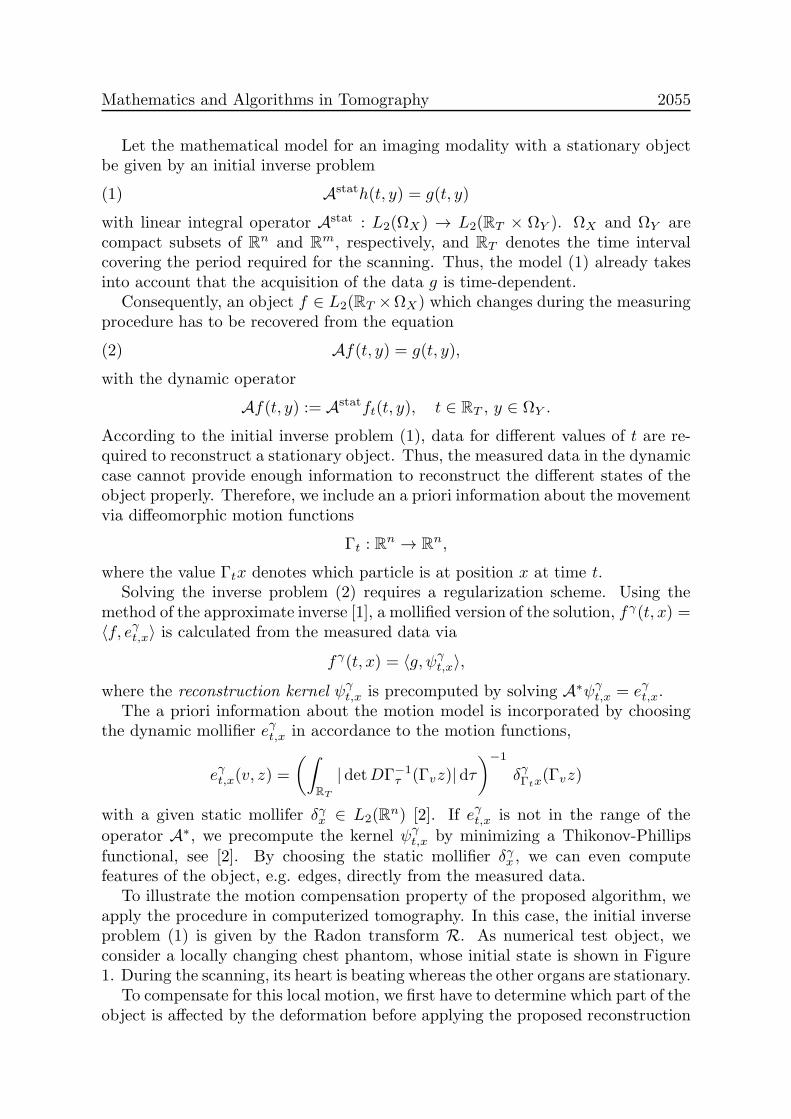
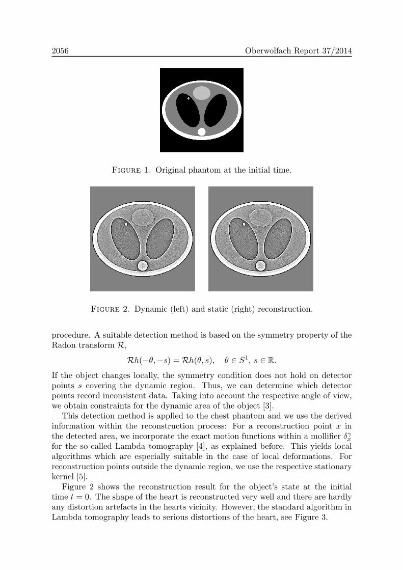
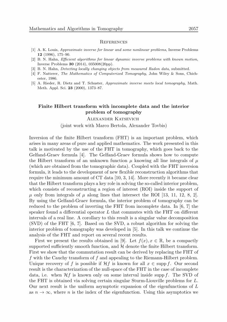
To illustrate the motion compensation property of the proposed algorithm, weapply the procedure in computerized tomography. In this case, the initial inverseproblem (1) is given by the Radon transform R. As numerical test object, weconsider a locally changing chest phantom, whose initial state is shown in Figure1. During the scanning, its heart is beating whereas the other organs are stationary.
To compensate for this local motion, we first have to determine which part of theobject is affected by the deformation before applying the proposed reconstruction
2056 Oberwolfach Report 37/2014
Figure 1. Original phantom at the initial time.
Figure 2. Dynamic (left) and static (right) reconstruction.
procedure. A suitable detection method is based on the symmetry property of theRadon transform R,
Rh(−θ,−s) = Rh(θ, s), θ ∈ S1, s ∈ R.
If the object changes locally, the symmetry condition does not hold on detectorpoints s covering the dynamic region. Thus, we can determine which detectorpoints record inconsistent data. Taking into account the respective angle of view,we obtain constraints for the dynamic area of the object [3].
This detection method is applied to the chest phantom and we use the derivedinformation within the reconstruction process: For a reconstruction point x inthe detected area, we incorporate the exact motion functions within a mollifier δγxfor the so-called Lambda tomography [4], as explained before. This yields localalgorithms which are especially suitable in the case of local deformations. Forreconstruction points outside the dynamic region, we use the respective stationarykernel [5].
Figure 2 shows the reconstruction result for the object’s state at the initialtime t = 0. The shape of the heart is reconstructed very well and there are hardlyany distortion artefacts in the hearts vicinity. However, the standard algorithm inLambda tomography leads to serious distortions of the heart, see Figure 3.
Mathematics and Algorithms in Tomography 2057
References
[1] A. K. Louis, Approximate inverse for linear and some nonlinear problems, Inverse Problems12 (1996), 175–90.
[2] B. N. Hahn, Efficient algorithms for linear dynamic inverse problems with known motion,Inverse Problems 30 (2014), 035008(20pp).
[3] B. N. Hahn, Detecting locally changing objects from measured Radon data, submitted.[4] F. Natterer, The Mathematics of Computerized Tomography, John Wiley & Sons, Chich-
ester, 1986.[5] A. Rieder, R. Dietz and T. Schuster, Approximate inverse meets local tomography, Math.
Meth. Appl. Sci. 23 (2000), 1373–87.
Finite Hilbert transform with incomplete data and the interior
problem of tomography
Alexander Katsevich
(joint work with Marco Bertola, Alexander Tovbis)
Inversion of the finite Hilbert transform (FHT) is an important problem, whicharises in many areas of pure and applied mathematics. The work presented in thistalk is motivated by the use of the FHT in tomography, which goes back to theGelfand-Graev formula [4]. The Gelfand-Graev formula shows how to computethe Hilbert transform of an unknown function µ knowing all line integrals of µ(which are obtained from the tomographic data). Coupled with the FHT inversionformula, it leads to the development of new flexible reconstruction algorithms thatrequire the minimum amount of CT data [10, 3, 14]. More recently it became clearthat the Hilbert transform plays a key role in solving the so-called interior problem,which consists of reconstructing a region of interest (ROI) inside the support ofµ only from integrals of µ along lines that intersect the ROI [13, 11, 12, 8, 2].By using the Gelfand-Graev formula, the interior problem of tomography can bereduced to the problem of inverting the FHT from incomplete data. In [6, 7] thespeaker found a differential operator L that commutes with the FHT on differentintervals of a real line. A corollary to this result is a singular value decomposition(SVD) of the FHT [6, 7]. Based on the SVD, a robust algorithm for solving theinterior problem of tomography was developed in [5]. In this talk we continue theanalysis of the FHT and report on several recent results.
First we present the results obtained in [9]. Let f(x), x ∈ R, be a compactlysupported sufficiently smooth function, and H denote the finite Hilbert transform.First we show that the commutation result can be derived by replacing the FHT off with the Cauchy transform of f and appealing to the Riemann-Hilbert problem.Unique recovery of f is possible if Hf is known for all x ∈ supp f . Our secondresult is the characterization of the null-space of the FHT in the case of incompletedata, i.e. when Hf is known only on some interval inside supp f . The SVD ofthe FHT is obtained via solving certain singular Sturm-Liouville problems for L.Our next result is the uniform asymptotic expansion of the eigenfunctions of Las n → ∞, where n is the index of the eigenfunction. Using this asymptotics we
2058 Oberwolfach Report 37/2014
derive the asymptotics of the singular values of the FHT in three different casesof incomplete data.
Next we present the results obtained in [1]. We study the asymptotics of singularvalues and singular functions of a Finite Hilbert transform (FHT), which is definedon several intervals. We suggest a novel approach based on the technique of thematrix Riemann-Hilbert problem and the steepest descent method of Deift-Zhou.We obtain a family of matrix RHPs depending on the spectral parameter λ andshow that the singular values of the FHT coincide with the values of λ for whichthe RHP is not solvable. Expressing the leading order solution as λ → 0 of theRHP in terms of the Riemann Theta functions, we prove that the asymptotics ofthe singular values can be obtained by studying the intersections of the locus ofzeroes of a certain Theta function with a straight line. This line can be calculatedexplicitly, and it depends on the geometry of the intervals that define the FHT.The leading order asymptotics of the singular functions and singular values areexplicitly expressed in terms of the Riemann Theta functions and of the periodmatrix of the corresponding normalized differentials, respectively. We also obtainthe error estimates for our asymptotic results.
References
[1] M. Bertola, A. Katsevich, and A. Tovbis, Singular value decomposition of a finite Hilberttransform defined on several intervals and the interior problem of tomography: theRiemann-Hilbert problem approach, Comm. Pure Appl. Math. accepted (2014), see alsoarXiv:1402.0216v1.
[2] M. Courdurier, F. Noo, M. Defrise, and H. Kudo, Solving the interior problem of computedtomography using a priori knowledge, Inverse Problems 24 (2008), Article ID 065001, 27pages.
[3] M. Defrise, F. Noo, R. Clackdoyle, and H. Kudo, Truncated Hilbert transform and imagereconstruction from limited tomographic data, Inverse Problems 22 (2006), 1037–1053.
[4] I. M. Gelfand and M. I. Graev, Crofton function and inversion formulas in real integralgeometry, Functional Analysis and its Applications 25 (1991), 1–5.
[5] X. Jin, A. Katsevich, H. Yu, G. Wang, , L. Li, and Z. Chen, Interior tomography withcontinuous singular value decomposition, IEEE Trans. Med. Imag. 31 (2012), 2108–2119.
[6] A. Katsevich, Singular value decomposition for the truncated Hilbert transform, InverseProblems 26 (2010), article ID 115011 (12 pp).
[7] , A note on computing the derivative at a constant direction, Physics in Medicineand Biology 56 (2011), N53–N61.
[8] H. Kudo, M. Courdurier, F. Noo, and M. Defrise, Tiny a priori knowledge solves the interiorproblem in computed tomography, Phys. Med. Biol. 53 (2008), 2207–2231.
[9] A. Katsevich and A. Tovbis, Finite Hilbert transform with incomplete data: null-space andsingular values, Inverse Problems 28 (2012), no. 10, Article ID 105006, 28 pages.
[10] F. Noo, R. Clackdoyle, and J. D. Pack, A two-step Hilbert transform method for 2D image
reconstruction, Physics in Medicine and Biology 49 (2004), 3903–3923.[11] Y. B. Ye, H. Y. Yu, and G. Wang, Exact interior reconstruction with cone-beam CT, Inter-
national Journal of Biomedical Imaging (2007), Article ID 10693.[12] , Local reconstruction using the truncated Hilbert transform via singular value de-
composition, Journal of X-Ray Science and Technology 16 (2008), 243–251.[13] Y. Ye, H. Yu, Y. Wei, and G. Wang, A general local reconstruction approach based on a
truncated Hilbert transform, International Journal of Biomedical Imaging (2007), Article ID63634.
Mathematics and Algorithms in Tomography 2059
[14] Y. Zou, X.C. Pan, and E.Y. Sidky, Image reconstruction in regions-of-interest from trun-cated projections in a reduced fan-beam scan, Physics in Medicine and Biology 50 (2005),13–27.
Inversion of the spherical means transform by reduction to the
classical Radon transform
Leonid Kunyansky
Thermo- and photo- acoustic tomography (TAT and PAT) aim to recover initialpressure of acoustic wave from pressure time series measured on a certain surfacepartially or completely surrounding the region of interest. The wave is incitedby illuminating the tissue with a very short laser pulse whose energy is partiallyabsorbed by the tissue, which slightly increases the temperature and causes ther-moacoustic expansion. The distribution of the initial pressure is closely related tothe conductivity of the tissue, allowing one to reconstruct high resolution imagesof vasculature or cancerous tumors.
We are interested in finding exact closed-form reconstruction formulas for theseimaging modalities. In addition to a clear theoretical insight, such formulas usu-ally result in simple and efficient algorithms that allow one to reconstruct theinitial pressure from the measured time series. In the context of thermo- andphoto-acoustic tomography, the existence of explicit inversion formulas dependson the measurement surface. In particular, exact closed-form reconstruction for-mulas have been obtained for planes, infinite cylinders, spheres and ellipsoids;cubes, certain triangles and tetrahedra; paraboloids and two-sheet hyperboloids,and some other, more complicated surfaces.
In the present work we consider corner-like acquisition geometries, such as aboundary of an octant Q ≡ x ∈ R3|x1 > 0, x2 > 0, x3 > 0 in 3D, or a boundaryof a quadrant in 2D. Inversion formulas for such surfaces are of interest since thecorresponding acquisition schemes are frequently used in practice. In particular, inorder to speed up the measurements, researchers utilize one-dimensional assembliesof detectors combined with acoustical lenses. In common use are also opticallyscanned glass plates whose surfaces play roles of arrays of acoustic sensors. Inorder to see all the material interfaces, such detectors have to surround the regionof interest (at least partially), resulting in the configurations considered here.
We assume that reflection of acoustic waves from the detectors is negligible.Such an assumption is realistic when detectors are small, or when a reflectedwave propagates away from detectors and vanishes at infinity. In particular, ifan optically scanned glass plate is used as a detector, the experiment should berepeated three times, with the glass plate placed in alternative positions. The useof several perpendicular glass plates simultaneously leads to occurrence of multiplereflections, and traditional TAT/PAT techniques are no longer applicable. Sucha situation is not covered by the present work and is considered by the authorelsewhere.
2060 Oberwolfach Report 37/2014
We present here the 3D version of the problem; the 2D version is simpler andcan be solved quite similarly. Under assumption of constant speed of sound (thatcan be set to 1 without loss of generality), acoustic pressure u(t, x) satisfies thewave equation
∆u = utt in R3, u(0, x) = f(x),∂u
∂t(0, x) = 0.
Initial pressure f(x) is supported within bounded region Ω lying within the oc-tant Q. Measurements g(t, z) coincide with pressure u(t, z) on boundary ∂Q ofQ (the boundary is a subset of the three coordinate planes). Using the retardedGreen’s function G(t, z − x) of the wave equation in R3 the measurements can beexpressed in the following form
g(t, z) =∂
∂t
∫
Ω
f(x)G(t, z − x)dx, G(t, x) =δ(t− |x|)
4π|x|,
where δ(t) is the Dirac’s delta-function.Consider the following combination of delta-functions supported on planes:
U(t, x) =
7∑
j=0
(−1)jδ(t− x · ωj),
where vectors ωj are multiple reflections the vector ω0 = (ω1, ω2, ω3) ∈ Q, andthe signs in the above formula are chosen so that the distribution U(t, x) is oddwith respect to each of the coordinates xj , j = 1, 2, 3. Let us denote by ∂Qj theintersection of ∂Q with the coordinate plane xj = 0, j = 1, 2, 3. Then it can beshown that the inner product of f(x) and Uδ(t, x, ω) can be expressed through themeasured data g(t, z) by the sum of the following three integrals:
∫
Q
f(x)Uδ(t, x, ω)dx = 2(ω1I1 + ω2I2 + ω3I3),(1)
I1 =
∫
∂Q1
[g(t+ y2ω3 + y3ω2, y) + g(t− y2ω3 − y3ω2, y)
− g(t+ y2ω3 − y3ω2, y)− g(t− y2ω3 + y3ω2, y)]dy,
where the expressions for integrals I2 and I3 are obtained from that for I1 bypermuting roles of y1, y2, and y3, and the roles of ω1, ω2, and ω3.
Further, one can show that inner product (1) coincides with the Radon trans-form of the odd part Of of f(x):
(ROf) (ω, t) ≡
∫
R3
δ(t− x · ω)Of(x)dx =
∫
R3
f(x)Uδ(t, x, ω)dx,
where Of(x) is defined as
Of(x) ≡ f(x)− f(R1x)−f(R2x) − f(R3x) + f(R2R1x) + f(R3R1x)
+ f(R3R2x)− f(R3R2R1x),

Mathematics and Algorithms in Tomography 2061
and where Rj are reflections of a vector with respect to coordinate planes xj =0, j = 1, 2, 3. Since f(x) is supported within Q, it can be reconstructed fromOf(x) simply by restricting values of x to Q. It follows that f(x) can be explicitlyreconstructed from the data g(t, z) by computing the values of the Radon transform(ROf) (ω, t) using formula (1), and by applying to the result any of the knowninversion formulas for the Radon transform in 3D.
ART Exhibit
Per Christian Hansen
In Kaczmarz’s formulation [6] of the algorithm from 1937, each iteration takes theform of a sweep over the rows aTi of the matrix A ∈ Rm×n – from top to bottom –where we orthogonally project the current iterate x on the hyperplane defined byrow aTi and the corresponding element bi of the right-hand side:
x← Pi x = x+bi − a
Ti x
‖ai‖22ai , i = 1, 2, . . . ,m .
Herman and his coworkers [3] rediscovered the algorithm 1970 (for the case whereall elements of A are 0 or 1). They named it “ART,” introduced a nonnegativityprojection and used a different normalization:
x← max
0 , x+
bi − aTi x
‖ai‖1ai
, i = 1, 2, . . . ,m .
This version does not have the simple interpretation as a sequence of orthogonalprojections; in later works (e.g., [5]) the name ART is used synonymously withthe Kaczmarz formulation. Current versions of ART also include a relaxationparameter λk and a projection PC on a convex set C (e.g., the positive orthant orthe box [0, 1]n):
x← PC
(x+ λk
bi − aTi x
‖ai‖22ai
), i = 1, 2, . . . ,m .
In spite of its success there are many open questions associated with the use ofthis method, and hence it is a rich source for research problems! Below two ofsome of these issues, with a strong bias towards my own research and my ongoingwork with the MATLAB package AIR Tools [4]. Please note the effort by JoostBatenburt from CWI to develop a highly efficient toolbox ASTRA [9], based on aMATLAB wrapper around native C++ and CUDA code.
Semi-Convergence Theory. There is a rich convergence theory for ART and itsmany block extensions; but most of this theory exclusively deals with its asymp-totic convergence. However, the power of ART really lies in its ability to convergefast to a good approximate/regularized solution during the initial iterations –while at later stages its slows down considerably and eventually converges to anundesirable solution dominated by noise from the data.
Specifically, ART is observed to exhibit semi-convergence [8], where the itera-tion number plays the role of the regularizing parameter. In the early stages the

2062 Oberwolfach Report 37/2014
iterates approach a regularized solution, while continuing the iteration leads toiterates deteriorated by noise. A few attempts have been made to give a rigorousfoundation for this observed behavior, such as [1]; but more work is needed todemonstrate in which circumstances we are guaranteed to have semi-convergence,to give rates for the initial convergence, etc.
Implementation of Block ART. There are surprisingly many ways to define blockextensions of ART; some of them are surveyed in [2] and [10]. These block methodslends themselves naturally to distributed computing systems and MPI-type imple-mentations for large-scale problems [7]. The block methods are also well suitedfor multi-core computers [10] as well as systems based on GPUs. Some importantquestions here are:
• How do we best choose the number of blocks on a given computer?• How can we best utilize the structural orthogonality between the matrixrows to choose the blocks adaptively?• What is the best combination of block iteration (sequential/parallel) andtreatment of the individual blocks (by a direct or iterative method)?
To best utilize the specialized architecture of the GPU, the matrix-free multi-plications are implemented such that the backprojection corresponds to multipli-
cation with the transposed of a matrix A that is slightly different from the matrixA associated with the forward computation [11]. The unmatched transpose mayprevent asymptotic convergence; it is unclear how it affects the semi-convergenceand the accuracy of the reconstruction.
References
[1] Elfving, P. C. Hansen, and T. Nikazad, Semi-convergence properties of Kaczmarzmethod, Inverse Problems, 30 (2014), DOI: 10.1088/0266-5611/30/5/055007.
[2] T. Elfving, T. Nikazad, and C. Popa, A class of iterative methods: semi-convergence,stopping rules, inconsistency, and constraining, in: Y. Censor, M. Jiang, and G. Wang(Eds.), Biomedical Mathematics: Promising Directions in Imaging, Therapy Planning, andInverse Problems, Medical Physics Publishing, Madison, WI, 2010.
[3] R. Gordon, R. Bender, G. T. Herman, Algebraic reconstruction techniques (ART) forthree-dimensional electron microscopy and X-ray photography, J. Theoretical Biology, 29(1970), pp. 477–481.
[4] P. C. Hansen and M. Saxild-Hansen, AIR Tools – A MATLAB package of alge-braic iterative reconstruction methods, J. Comp. Appl. Math., 236 (2012), pp. 2167–2178,DOI: 10.1016/j.cam. 2011.09.039.
[5] G. T. Herman, Fundamentals of Computerized Tomography: Image Reconstruction from
Projections, 2. Ed., Springer, New York, USA, 2009.[6] S. Kaczmarz, Angenaherte Auflosung von Systemen linearer Gleichungen, Bull. Acad. Pol.
Sci. Lett., A35 (1937), pp. 355–357.[7] N. T. Karonis, K. L. Duffin, C. E. Ordonez, B. Erdelyi, T. D. Uram, E. C. Olson,
G. Coutrakon, M. E. Papka, Distributed and hardware accelerated computing for clinicalmedical imaging using proton computed tomography (pCT), J. Parallel Distrib. Comput.,73 (2013), pp. 1605–1612.
[8] F. Natterer, The Mathematics of Computerized Tomography, SIAM, Philadelphia, 2001.
Mathematics and Algorithms in Tomography 2063
[9] W J. Palenstijn, K J. Batenburg, and J. Sijbers, Performance improvements for iter-ative electron tomography reconstruction using graphics processing units (GPUs), J. Struc-tural Biology, 176 (2011), pp. 250–253.
[10] H. H. B. Sørensen and P. C. Hansen, Multi-core performance of block algebraic iterativereconstruction methods, SIAM J. Sci. Comp., to appear.
[11] G. L. Zeng and G. T. Gullberg, Unmatched projector/backprojector pairs in an iterativereconstruction algorithm, IEEE Trans. Medical Imag., 19 (2000), pp. 548–555.
Monostatic SAR with Fold-Cusp Singularities
Clifford Nolan
(joint work with Raluca Felea)
In this talk we reported on preliminary work on imaging terrain using SyntheticAperture Radar (SAR) where the flight track of the Radar follows a curve whosecurvature is only allowed to vanish simply. For a microlocal review of SAR, see [1]and for related technical tools, see [3].
This work is a natural progression from [2] where the curvature of the flighttrack either (i) never vanishes or else (ii) is identically zero. In both cases (i) and(ii), the natural projections (πL, πR) from the wavefront relation Λ of the forwardmodelling (scattering) operator F into the cotangent space of the data (T ∗Y ) andthe cotangent space of the model (T ∗X) respectively have singularities. In bothcase (i) and (ii) we have that πL has a fold singularity. On the other hand, wehave that the πR projection has a fold singularity in case (i) and a blowdownsingularity in case (ii). Both cases lead to artifacts in the backprojected image.This is reflected mathematically by showing that the Schwartz kernel of F∗F is apaired Lagrangian distribution associated to the diagonal and a non-diagonalcanonincal relation Λ (responsible for the artifacts).
In this current work [4], we investigate what happens in the intermediate casewhere the curvature is allowed to vanish but only simply. We establish that theSchwartz kernel of F∗F is no longer a paired Lagrangian distribution. We alsoshow that artifacts are still present as this is intuitively clear if one considers say asinusoid flight track with an inflexion point where the curvature vanishes simply.Now this flight track consists of two open curves where the curvature is never zerotogether with the inflexion point itself. Therefore we expect to obtain the artifactspredicted by [2].
We also develop a weak normal form for the phase function of the Fourierintegral operator F in the case of simply vanishing curvature and we use it toprove the results in the previous paragraph in a more general setting for any FIOwith fold/cusp singularites.
References
[1] C.J. Nolan & M. Cheney. Synthetic Aperture inversion. Inverse Problems. an InternationalJournal on the Theory and Practice of Inverse Problems, Inverse Methods and Computer-ized Inversion of Data , 18(1), (2002), 221–235.
2064 Oberwolfach Report 37/2014
[2] C.J. Nolan & M. Cheney. Microlocal analysis of synthetic aperture radar imaging. TheJournal of Fourier Analysis and Applications, 10(2), (2004), 133–148.
[3] R. Felea, Composition of Fourier integral operators with fold and blowdown singularities.Communications in Partial Differential Equations, 30(10-12), (2005), 1717–1740.
[4] R. Felea, C. Nolan, Monostatic SAR with fold/cusp singularities. Submitted
Artifacts in limited view tomography
Jurgen Frikel
(joint work with Eric Todd Quinto)
Introduction. In many tomographic imaging scenarios the measured data is avail-able only from a limited range of view. As a consequence, only specific featuresof the unknown object can be reconstructed reliably [11] and added artifacts canbe generated [2, 6]. The added artifacts can degrade the image quality and com-plicate an accurate interpretation of images. It is therefore essential to developa mathematical understanding of these phenomena and to derive artifact reduc-tion strategies that can be easily incorporated into widely used reconstructionalgorithms. Here, we consider filtered backprojection type reconstructions fromlimited view data and present a paradigm to characterize visible and added sin-gularities (artifacts). Our methodology is based on the framework of microlocalanalysis and the calculus of Fourier integral operators. Particularly, we presentcharacterizations of visible and added singularities for limited angle x-ray andphotoacoustic tomography reconstructions.
The presented results were obtained in our recent works [2, 3]. For x-ray lambdatomography similar results were obtained in [6]. Recently, L. Nguyen has analyzedthe strength of the added artifacts generated in reconstructions from limited angleRadon transform and spherical Radon transform data [9, 10].
Microlocal analysis of general limited data problems. In what follows, weassume that the forward operator T : E ′(Ω)→ E ′(Ξ) is a Fourier Integral operator(FIO), where Ω denotes the object space and Ξ is the data space. The limited datareconstruction problem consists in recovering a function f (or an approximation)from the data g(y) = Tf(y) on a restricted subset A of the data space, i.e.,y ∈ A ( Ξ. Therefore, the limited view forward operator is given by TAf = χATf ,where χA denotes the characteristic function of A. In cases we consider, thereconstruction operators B are of filtered backprojection (FBP) type:
BgA = T ∗PgA, gA = TAf,
where P is a pseudodifferential operator and T ∗ is the dual (or backprojection)operator to T .
To understand visible and added singularities of BgA = T ∗PTAf , our goal is tocalculate WF(T ∗P TAf), where WF(u) denotes the wavefront set [4]. Before wecan start the calculations, we first need to check that the product TAf = χATf iswell-defined in the sense of distributions. This can be done by making sure thatthe non-cancellation condition holds for χA and Tf , i.e., (y, ξ) ∈ WF(Tf) ⇔

Mathematics and Algorithms in Tomography 2065
(y,−ξ) /∈ WF(χA). In the next step we apply the Hormander Sato lemma [12]which states that if T is a FIO and C its associated canonical relation, thenWF(Tf) ⊂ C WF(f) = (y, ηdy) : ∃(x, ξdx) ∈WF(f) : (y, ηdy;x, ξdx) ∈ C.Furthermore, by noting that T ∗ is a FIO associated to the canonical relationCt = (y, ηdy;x, ξdx) : (x, ξdx; y, ηdy) ∈ C [12], we conclude that
WF(T ∗P TAf) ⊂ Ct WF(P TAf) ⊂ C
t WF(TAf).
The latter inclusion follows from the pseudolocal property of pseudodifferentialoperators [12]. To compute visible and added singularities we eventually need tocompute the set WF(TAf) and the composition Ct WF(TAf). For more detailswe refer to [3].
Visible and added singularities in x-ray and photoacoustic tomography.
We consider the classical Radon transform R : E ′(Ω)→ E ′([0, 2π]×R) as a forwardoperator for x-ray tomography, [8], and the limited angle data set A = [a, b]× R.The circular Radon transform M : E ′(Ω) → E ′([0, 2π] × (0,∞)) is a standardforward operator for photoacoustic tomography, [1, 7], which we study with thelimited angle data set A = [a, b]× (0,∞). The next theorem shows explicitly thatthe Radon transforms detect singularities conormal to the set being integrated over(cf. [5]), and that added artifacts can appear only on lines (forR) or circles (forM),respectively, that are conormal to singularities of f with directions correspondingto the boundary of the angular range [a, b].
Theorem 1 ([2, 3]). Let T ∈ R,M, f ∈ E ′(Ω), and let P be a pseudodifferentialoperator on D′(Ξ). Then,
WF(T ∗PTAf) ⊂WF[a,b](f) ∪Aa,b(f),
where WF[a,b](f) := WF(f)∩V[a,b] ⊂WF(f) is the set of visible singularities andAa,b(f) is the set of possible added singularities. Let θ(φ) = (cosφ, sinφ) and
θ⊥(φ) = (− sinφ, cosφ), then we have for the classical Radon transform R:
V[a,b] = (x, ξdx) ∈ T∗(Ω): α 6= 0, φ ∈ [a, b]
A[a,b](f) = (x+ tθ⊥(φ), αθ(φ)dx) : φ ∈ a, b,
α, t 6= 0, x ∈ L(φ, s), (x, αθ(φ)) ∈WF(f)
whereas for the circular Radon transform M we have:
V[a,b] = (x, ξdx) ∈ T∗(Ω): ∃φ ∈ [a, b], ∃α 6= 0, ξ = α(x − θ(φ))
Aa,b(f) =(x, d(x − θ(φ)dx) : x ∈ Ω, φ ∈ a, b,
∃x′ ∈ C (φ, ‖x− θ(φ)‖), (x′, d(x′ − θ(φ))dx) ∈WF (f)
The next theorem shows that no added singularities are introduced in the re-construction if the limited view data is smoothly truncated at the boundary of theangular range.
Theorem 2 ([2, 3]). Let T ∈ R,M and let κ : [0, 2π]→ R be a smooth functionsuch that supp(κ) ⊂ [a, b]. Let K be the operator defined by Kg(φ, s) = κ(φ)g(φ, s).
2066 Oberwolfach Report 37/2014
Then, the operator T ∗P KTA is a standard pseudodifferential operator and forf ∈ E ′(D),
WF(T ∗P K(TAf ) ) ⊂WF[a,b](f),
where WF[a,b](f) is the corresponding set of visible singularities given above.
References
[1] P. Elbau, O. Scherzer and R. Schulze, Reconstruction formulas for photoacoustic sectionalimaging, Inverse Problems 28(4): 045004, 2012.
[2] J. Frikel and E. T. Quinto, Characterization and reduction of artifacts in limited angletomography, Inverse Problems 29(12): 125007, 2013.
[3] J. Frikel and E. T. Quinto, Artifacts in incomplete data tomography - with applications tophotoacoustic tomography and sonar, arXiv:1407.3453 [math.AP], 2014.
[4] L. Hormander, The analysis of linear partial differential operators. I, Springer-Verlag,Berlin, 2003.
[5] V. Guillemin and S. Sternberg, Geometric Asymptotics, American Mathematical Society,Providence, RI, 1977.
[6] A. Katsevich, Local tomography for the limited-angle problem, J. Math. Anal. Appl. 213(1):160-182, 1997.
[7] P. Kuchment and L. Kunyansky, Mathematics of photoacoustic and thermoacoustic tomog-raphy, in Handbook of Mathematical Methods in Imaging, Otmar Scherzer, ed., Springer,2010, pp. 817-866.
[8] F. Natterer, The mathematics of computerized tomography, B. G. Teubner, Stuttgart, 1986.[9] L. Nguyen, How strong are streak artifacts in limited angle computed tomography?,
arXiv:1407.3037 [math.CA], 2014.[10] L. Nguyen, On Artifacts in Limited Data Spherical Radon Transform, Preprint, 2014.[11] E. T. Quinto, Singularities of the X-ray transform and limited data tomography in R2 and
R3, SIAM Journal on Mathematical Analysis 24(5): 1215–1225, 1993.[12] F. Treves, Introduction to Pseudodifferential and Fourier Integral Operators, Volume 2:
Fourier Integral Operators, Plenum Press, New York and London, 1980.
Boundary rigidity and lens rigidity
Gunther Uhlmann
Abstract
We survey some recent results on the boundary rigidity problem with partial databased on [40]. The local result leads to a global result for the lens rigidity problem.
The boundary rigidity problem with partial data
Travel time tomography deals with the problem of determining the sound speedor index of refraction of a medium by measuring the travel times of waves goingthrough the medium. This type of inverse problem, also called the inverse kine-matic problem, arose in geophysics in an attempt to determine the substructureof the Earth by measuring the travel times of seismic waves at the surface. Weconsider an anisotropic index of refraction, that is the sound speed depends onthe direction. The Earth is generally anisotropic. More recently it has been re-alized, by measuring these travel times, that the inner core of the Earth exhibits

Mathematics and Algorithms in Tomography 2067
anisotropic behavior with the fast direction parallel to the Earth’s spin axis, see[4]. In the human body, muscle tissue is anisotropic. As a model of anisotropy, weconsider a Riemannian metric g = (gij). The problem is to determine the metricfrom the lengths of geodesics joining points on the boundary.
This leads to the general question of whether given a compact Riemannianmanifold with boundary (M, g) one can determine the Riemannian metric in theinterior knowing the boundary distance function joining points on the bound-ary dg(x, y), with x, y ∈ ∂M. This is known as the boundary rigidity problem.Of course, isometries preserve distance, so that the boundary rigidity problem iswhether two metrics that have the same boundary distance function are the sameup to isometry. Examples can be given of manifolds that are not boundary rigid.Such examples show that the boundary rigidity problem should be considered un-der some restrictions on the geometry of the manifold. The most usual of suchrestrictions is simplicity of the metric. A Riemannian manifold (M, g) (or the met-ric g) is called simple if the boundary ∂M is strictly convex and any two pointsx, y ∈M are joined by a unique minimizing geodesic. Michel conjectured [17] thatevery simple compact Riemannian manifold with boundary is boundary rigid.
Simple surfaces with boundary are boundary rigid [24]. In higher dimensions,simple Riemannian manifolds with boundary are boundary rigid under some a-priori constant curvature on the manifold or special symmetries [1], [9]. Severallocal results near the Euclidean metric are known [32], [15], [2]. The most generalresult in this direction is the generic local (with respect to the metric) one provenin [34]. Surveys of some of the results can be found in [12], [35], [7].
The paper [40] considers the boundary rigidity problem in the class of metricsconformal to a given one and with partial data, that is, we know the boundarydistance function for points on the boundary near a given point. Partial dataproblems arise naturally in applications since in many cases one doesn’t have accessto the whole boundary. In [40] it is proven the first result on the determination ofthe conformal factor locally near the boundary from partial data without assuminganalyticity.
We now describe the known results with full data on the boundary. Let us fixthe metric g0 and let c be a positive smooth function on the compact manifold withboundaryM . The problem is whether we can determine c from dc−2g0(x, y), x, y ∈∂M. Notice that in this case the problem is not invariant under changes of variablesthat are the identity at the boundary so that we expect to be able to recover cunder appropriate a-priori conditions. This was proven by Mukhometov in twodimensions [19], and in [20] in higher dimensions for the case of simple metrics. Ofparticular importance in applications is the case of an isotropic sound speed thatis when we are in a bounded domain of Euclidean space and g0 is the Euclideanmetric. This is the isotropic case. This problem was considered by Herglotz [10]and Wieckert and Zoeppritz [43] for the case of a spherical symmetric sound speed.They found a formula to recover the sound speed from the boundary distancefunction assuming d
dr (r
c(r)) > 0. Notice that this condition is equivalent in the
radial case to non-trapping and is more general than simplicity.
2068 Oberwolfach Report 37/2014
From now on we will call d the function dc−2g0 .It is shown in [40] the following uniqueness result:
Theorem 3. Let n = dimM ≥ 3, let c > 0, c > 0 be smooth and let ∂M bestrictly convex with respect to both g = c−2g0 and g = c−2g0 near a fixed p ∈ ∂M .Let d(p1, p2) = d(p1, p2) for p1, p2 on ∂M near p. Then c = c in M near p.
This is the only known result for the boundary rigidity problem with partialdata except in the case that the metrics are assumed to be real-analytic [15]. Thelatter follows from determination of the jet of the metric at a convex point fromthe distance function known near p.
Lens rigidity
The boundary rigidity problem is closely connected to the lens rigidity one. Todefine the latter, we first introduce the manifolds ∂±SM , defined as the sets of allvectors (x, v) with x ∈ ∂M , v unit in the metric g, and pointing outside/insideM . We define the lens relation
(1) L : ∂−SM −→ ∂+SM
in the following way: for each (x, v) ∈ ∂−SM , L(x, v) = (y, w), where y is the exitpoint, and w the exit direction, if exist, of the maximal unit speed geodesic γx,vin the metric g, issued from (x, v). Let
ℓ : ∂−SM −→ R ∪∞
be its length, possibly infinite. If ℓ <∞, we call M non-trapping.The lens rigidity problem is whether the lens relation L (and possibly, ℓ) de-
termine g (and the topology of M) up to an isometry as above. The lens rigidityproblem with partial data for a sound speed is whether we can determine the speednear some p from L known near Sp∂M . For general metrics, we want to recoverisometric copies of the metrics locally, as above.
We assume that ∂M is strictly convex at p ∈ ∂M w.r.t. g. Then the boundaryrigidity and the lens rigidity problems with partial data are equivalent: knowingd near (p, p) is equivalent to knowing L in some neighborhood of Sp∂M . The sizeof that neighborhood however depends on a priori bounds of the derivatives of themetrics with which we work. This equivalence was first noted by Michel [17], sincethe tangential gradients of d(x, y) on ∂M × ∂M give us the tangential projectionsof −v and w, see also [31, sec. 2]. Note that local knowledge of ℓ is not needed foreither problems, and in fact, ℓ can be recovered locally from either d or ℓ.
Vargo [42] proved that real-analytic manifolds satisfying an additional mildcondition are lens rigid. Croke has shown that if a manifold is lens rigid, a finitequotient of it is also lens rigid [7]. He has also shown that the torus is lens rigid[3]. G. Uhlmann and P. Stefanov have shown lens rigidity locally near a genericclass of non-simple manifolds [37]. The only result we know for the lens rigidityproblem with partial data is for real-analytic metric satisfying a mild condition[37]. While in [37], the lens relation is assumed to be known on a subset only, the

Mathematics and Algorithms in Tomography 2069
geodesics issued from that subset cover the whole manifold. In contrast, in [40],we have localized information.
The linearization of the boundary rigidity and lens rigidity problem is the tensortomography problem, i.e., recovery of a tensor field up to “potential fields” fromintegrals along geodesics joining points on the boundary. It has been extensivelystudied in the literature for both simple and non-simple manifolds [8, 21, 22,23, 18, 25, 30, 27, 33, 36, 39]. See the book [28] and [23] for a recent survey.The local tensor tomography problem has been considered in [13] for functionsand real-analytic metrics and in [14] for tensors of order two and real-analyticmetrics. Those results can also be thought of as support theorems of Helgason type.The only known results for the local problem for smooth metrics and integrals offunctions is [41]. In [44] this type of result was proven for more general curvesthan geodesics and more general weights using similar methods.
Now we use a layer stripping type argument to obtain a global result which isdifferent from Mukhometov’s for simple manifolds.
Definition 1. Let (M, g) be a compact Riemannian manifold with boundary. Wesay that M satisfies the foliation condition by strictly convex hypersurfaces if Mis equipped with a smooth function ρ : M → [0,∞) which level sets Σt = ρ−1(t),t < T with some T > 0 are strictly convex viewed from ρ−1((0, t)) for g, dρ isnon-zero on these level sets, and Σ0 = ∂M and M \∪t∈[0,T )Σt has empty interior.
The statement of the global result on lens rigidity proven in [40] is as follows:
Theorem 4. Let n = dimM ≥ 3, let c > 0, c > 0 be smooth and equal on ∂M ,let ∂M be strictly convex with respect to both g = c−2g0 and g = c−2g0. Assumethat M can be foliated by strictly convex hypersurfaces for g. Then if L = L on∂−SM , we have c = c in M .
A more general foliation condition under which the theorem would still hold isformulated in [38]. In particular, Σ0 does not need to be ∂M and one can haveseveral such foliations with the property that the closure of their union isM . If wecan foliate only some connected neighborhood of ∂M , we would get c = c there.Note that it is enough to require that M \ ∪t∈[0,T )Σt is simple to prove c = c in∪t∈[0,T )Σt first, and then use Mukhometov’s results to complete the proof. Theclass of manifolds we get in this way is larger than the simple ones.
Spherically symmetric c(x) under the condition considered by Herglotz andWieckert and Zoeppritz satisfy the foliation condition of the theorem. Other ex-amples of non-simple metrics that satisfy the condition are the tubular neighbor-hood of a closed geodesic in negative curvature. These have trapped geodesics.Also the rotationally symmetric spaces on the ball with convex spheres can be farfrom simple. It follows from the result of [26], that manifolds with no focal pointssatisfy the foliation condition. It would be interesting to know whether this is alsothe case for simple manifolds. As it was mentioned earlier manifolds satisfying thefoliation condition are not necessarily simple.
The linearization of the non-linear problem with partial data considered in The-orem 3 was considered in [41], where uniqueness and stability were shown. This

2070 Oberwolfach Report 37/2014
corresponds to integrating functions along geodesics joining points in a neighbor-hood of p. The method of proof of Theorem relies on using an identity provenin [32] to reduce the problem to a ”pseudo-linear” one: to show uniqueness whenone integrates the function f = and its derivatives on the geodesics for the met-ric g joining points near p, with weight depending non-linearly on both g and g.Notice that this is not a proof by linearization, and unlike the problem with fulldata, an attempt to do such a proof is connected with essential difficulties. Theproof of uniqueness for this linear transform follows the method of [41] introduc-ing an artificial boundary and using Melrose’ scattering calculus. The we use themethod of [32] to reduce the problem to a “pseudo-linear problem” and applysimilar techniques to [41].
Stability estimates
In Theorem 5 and Theorem 6 were proven in [40] giving a Holder conditionalstability estimates of local and then of global type respectively. In case of dataon the whole boundary, such an estimate was proved in [34, section 7] for simplemanifolds and metrics not necessarily conformal to each other. Below, the Ck
norm is defined in a fixed coordinate system in the local result, and with respectto a fixed finite collection of local chart in the global case.
Theorem 5. There exists k > 0 and 0 < µ < 1 with the following property. Forany 0 < c0 ∈ C
k(M), p ∈ ∂M , and A > 0, there exists ε0 > 0 and C > 0 with theproperty that for any two positive c, c with
(2) ‖c− c0‖C2 + ‖c− c0‖C2 ≤ ε0, and ‖c‖Ck + ‖c‖Ck ≤ A, j = 1, 2,
and for any neighborhood Γ of p on ∂M , we have the stability estimate
(3) ‖c− c‖C2(U) ≤ ‖d− d‖µC(Γ×Γ)
for some neighborhood U of p in M .
The global estimate for the lens rigidity problem assuming the foliation condi-tion is as follows:
Theorem 6. Assume that M0 ⊂ M can be foliated by strictly convex hyper-surfaces. Let D ⊂ ∂−SM be a neighborhood of the compact set of all β ∈∂−SM ∩ ∂−SM0 with the property that the geodesic γβ stays in M0 and hits ∂Magain at a point on ∂M0. Then with k, µ, c0, c, c, ε0 and A as in Theorem 5, wehave the stability estimate
(4) ‖c− c‖C2(M0) ≤ C‖L− L‖µC(D)
for c1, c2 satisfying (2).
The quantity L− L, and its C(D) norm make sense in a finite system of chartscovering ∂M .
Acknowledgement
The Author was partly supported by the NSF and a Simons Fellowship.
Mathematics and Algorithms in Tomography 2071
References
[1] G. Besson, G. Courtois, and S. Gallot. Entropies et rigidites des espaces localementsymetriques de courbure strictment negative. Geom. Funct. Anal., 5 (1995), 731–799.
[2] D. Burago and S. Ivanov, Boundary rigidity and filling volume minimality of metrics closeto a flat one. Ann. Math., 171 (2010), 1183–1211.
[3] C. Croke. Scattering rigidity with trapped geodesics. preprint, 2012.[4] K. C. Creager. Anisotropy of the inner core from differential travel times of the phases PKP
and PKIPK, Nature, 356(1992), 309–314.[5] C. B. Croke. Rigidity for surfaces of nonpositive curvature. Comment. Math. Helv.,
65(1):150–169, 1990.[6] C. B. Croke. Rigidity and the distance between boundary points. J. Differential Geom.,
33(2):445–464, 1991.[7] C. B. Croke. Rigidity theorems in Riemannian geometry. In Geometric methods in inverse
problems and PDE control, volume 137 of IMA Vol. Math. Appl., pages 47–72. Springer,New York, 2004.
[8] N. S. Dairbekov. Integral geometry problem for nontrapping manifolds. Inverse Problems,22(2):431–445, 2006.
[9] M. Gromov. Filling Riemannian manifolds. J. Diff. Geometry 18 (1983), 1–148.
[10] G. Herglotz. Uber die Elastizitaet der Erde bei Beruecksichtigung ihrer variablen Dichte.Zeitschr. fur Math. Phys., 52:275–299, 1905.
[11] L. Hormander. The analysis of linear partial differential operators, vol. 1-4. Springer-Verlag,1983.
[12] S. Ivanov. Volume comparison via boundary distances. Proceedings of the InternationalCongress of Mathematicians, vol. II, 769–784, New Delhi, 2010.
[13] V. Krishnan. A support theorem for the geodesic ray transform on functions. J. FourierAnal. Appl. 15 (2009), 515–520.
[14] V. Krishnan and P. Stefanov. A support theorem for the geodesic ray transform of symmetrictensor fields. Inverse Problems and Imaging, 3 (2009), 453–464.
[15] M. Lassas, V. Sharafutdinov, and G. Uhlmann. Semiglobal boundary rigidity for Riemannianmetrics. Math. Ann., 325(4):767–793, 2003.
[16] R. B. Melrose. Spectral and scattering theory for the Laplacian on asymptotically Euclidianspaces. Spectral and scattering theory (Sanda, 1992). Lecture Notes in Pure and Appl.Math., 161, 85–130, Marcel Dekker, 1994.
[17] R. Michel. Sur la rigidite imposee par la longueur des geodesiques. Invent. Math., 65(1):71–83, 1981/82.
[18] R. G. Mukhometov. The reconstruction problem of a two-dimensional Riemannian metric,and integral geometry. Dokl. Akad. Nauk SSSR, 232(1):32–35, 1977.
[19] R. G. Muhometov. On a problem of reconstructing Riemannian metrics. Sibirsk. Mat. Zh.,22(3):119–135, 237, 1981.
[20] R. G. Muhometov and V. G. Romanov. On the problem of finding an isotropic Riemannianmetric in an n-dimensional space. Dokl. Akad. Nauk SSSR, 243(1):41–44, 1978.
[21] G.P. Paternain, M. Salo and G. Uhlmann. Tensor tomography on simple surfaces, Invent.
Math., 193(2013), 229-247.[22] G.P. Paternain, M. Salo, G. Uhlmann. The attenuated ray transform for connections and
Higgs fields, Geom. Funct. Anal. 22 (2012) 1460–1489.[23] G.P. Paternain, M. Salo and G. Uhlmann. Tensor tomography: progress and challenges,
preprint, arXiv:1303.6114.[24] L. Pestov and G. Uhlmann. Two dimensional compact simple Riemannian manifolds are
boundary distance rigid. Ann. of Math. (2), 161(2):1093–1110, 2005.[25] L. N. Pestov and V. A. Sharafutdinov. Integral geometry of tensor fields on a manifold of
negative curvature. Sibirsk. Mat. Zh., 29(3):114–130, 221, 1988.
2072 Oberwolfach Report 37/2014
[26] A. Ranjan and H. Shah. Convexity of spheres in a manifold without conjugate points. Proc.Indian Acad. Sci. (Math. Sci.), 112 (2002), 595–599.
[27] V. Sharafutdinov, M. Skokan, and G. Uhlmann. Regularity of ghosts in tensor tomography.J. Geom. Anal., 15(3):499–542, 2005.
[28] V. A. Sharafutdinov. Integral geometry of tensor fields. Inverse and Ill-posed ProblemsSeries. VSP, Utrecht, 1994.
[29] V. A. Sharafutdinov. A problem in integral geometry in a nonconvex domain. Sibirsk. Mat.Zh., 43(6):1430–1442, 2002.
[30] V.A. Sharafutdinov,Variations of Dirichlet-to-Neumann map and deformation boundaryrigidity of simple 2-manifolds, J. Geom. Anal. 17 (2007), 147–187.
[31] P. Stefanov. Microlocal approach to tensor tomography and boundary and lens rigidity.Serdica Math. J., 34(1):67–112, 2008.
[32] P. Stefanov and G. Uhlmann. Rigidity for metrics with the same lengths of geodesics. Math.Res. Lett., 5(1-2):83–96, 1998.
[33] P. Stefanov and G. Uhlmann. Stability estimates for the X-ray transform of tensor fieldsand boundary rigidity. Duke Math. J., 123(3):445–467, 2004.
[34] P. Stefanov and G. Uhlmann. Boundary rigidity and stability for generic simple metrics. J.Amer. Math. Soc., 18(4):975–1003, 2005.
[35] P. Stefanov and G. Uhlmann. Boundary and lens rigidity, tensor tomography and analyticmicrolocal analysis. In Algebraic Analysis of Differential Equations. Springer, 2008.
[36] P. Stefanov and G. Uhlmann. Integral geometry of tensor fields on a class of non-simpleRiemannian manifolds. Amer. J. Math., 130(1):239–268, 2008.
[37] P. Stefanov and G. Uhlmann. Local lens rigidity with incomplete data for a class of non-simple Riemannian manifolds. J. Differential Geom., 82(2):383–409, 2009.
[38] P. Stefanov and G. Uhlmann. Recovery of a source term or a speed with one measurementand applications, Trans. Amer. Math. Soc., 365, 5737-5758, 2013.
[39] P. Stefanov and G. Uhlmann. The geodesic X-ray transform with fold caustics. Anal. PDE,5, 219–260, 2012.
[40] P. Stefanov, G. Uhlmann and A. Vasy, Boundary rigidity with partial data, preprint,arXiv:1306.2995.
[41] G. Uhlmann and A. Vasy. The inverse problem for the local geodesic ray transform. preprint,arXiv:1210.2084.
[42] J. Vargo. A proof of lens rigidity in the category of analytic metrics, Math. Research Letters,16 (2009), 1057–1069.
[43] E. Wiechert and K. Zoeppritz. Uber Erdbebenwellen. Nachr. Koenigl. Geselschaft Wiss.Gottingen, 4:415–549, 1907.
[44] H. Zhou. The inverse problem for the local ray transform. Preprint. arXiv:1304.7023, 2013.
Tomography of small residual stresses
Vladimir Sharafutdinov
(joint work with Jenn-Nan Wang)
We study the inverse problem of determining the residual stress in Man’s model [1]using tomographic data. Theoretically, the tomographic data are obtained at thezeroth approximation of geometrical optics for Man’s residual stress model. Forcompressional waves, the inverse problem is equivalent to the problem of invertingthe longitudinal ray transform of a symmetric tensor field. For shear waves, the in-verse problem, after the linearization, leads to another integral geometry operatorwhich is called the mixed ray transform. Under some restrictions on coefficients,we are able to prove the uniqueness results in these two cases.

Mathematics and Algorithms in Tomography 2073
References
[1] C.-S. Man. Hartig’s law and linear elasticity with initial stress, Inverse Problems 14 (1998),313–319.
Some steps in making tomography algorithms practical
Kees Joost Batenburg
In the past decades, X-ray tomography has developed into an advanced field ofexperimental research, utilizing not just the absorption contrast, but also phase,chemical and directional information to characterize the interior structure of thescanned object. Achieving the best possible results is becoming more and more aninterdisciplinary effort, combining state-of-the-art experimental hardware, care-ful experiment design, mathematical modeling, customized algorithms and highperformance computing.
One of the key challenges is to obtain accurate reconstructions from a limitedset of measurements (a small number of projections, limited angular range, etc.).In this domain, recent mathematical advances in incorporating various types ofprior knowledge in the reconstruction algorithm have the potential to provide vastimprovements in image quality.
However, it is not at all straightforward to translate advanced numerical al-gorithms into a software implementation that can be applied effectively to largeexperimental datasets. In particular
• Practical data sets are often extremely large, requiring highly efficientparallel processing and efficient memory usage.• A broad range of geometrical projection configurations is used in modernexperiments, such that algorithms based on particular geometries (e.g.parallel beam, circular cone beam) can often not be used.• A broad collection of structural errors and uncertainties introduced duringimage acquisition (alignment errors, flat field fluctuations, etc.) imposestrong requirements on the robustness of the algorithm with respect tomodel errors.
At the Computational Imaging group of CWI (Amsterdam, The Netherlands)and the ASTRA group at the University of Antwerp (Belgium), we aim to de-velop methodologies that allow to bridge this gap between advanced mathemati-cal algorithms and real-world experimental data. In particular, we have developedthe ASTRA toolbox, an open-source software toolbox that offers flexible, high-performance GPU implementations of the tomographic forward and back projec-tion operators [1, 2]. Through an interface with high-level scripting languages(Matlab and Python), algorithms can be expressed in an intuitive mathematicalway, while being directly applicable to large experimental datasets.
2074 Oberwolfach Report 37/2014
References
[1] W.J. Palenstijn, K.J. Batenburg, and J. Sijbers, The ASTRA tomography toolbox, 13thInternational Conference on Computational and Mathematical Methods in Science and En-gineering, CMMSE, (2013). http://sourceforge.net/projects/astra-toolbox/.
[2] W.J. Palenstijn, K.J. Batenburg, and J. Sijbers, Performance improvements for iterativeelectron tomography reconstruction using graphics processing units (GPUs)., Journal ofStructural Biology, 176(2) (2011), 250–253.
Simultaneous estimation of attenuation and activity in time-of-flight
positron emission tomography.
Michel Defrise
(joint work with J. Nuyts, A. Rezaei, V. Panin, M. Caey, C. Michel, G. Bal, C.Watson, M. Conti)
Positron emission tomography (PET) aims at estimating the spatial distributionof a tracer labelled with a positron emitting isotope. This distribution, calledthe activity image λ, is reconstructed from the emission data m, which consistof pairs of 511 keV photons detected in coincidence by detectors surrounding thepatient. An accurate reconstruction requires in addition information on the spatialdistribution of the attenuation coefficient, (the attenuation image µ), which isneeded to compensate for the absorption or scattering of the photons.
In practice the attenuation is measured independently using a CT scan (x-raytransmission tomography). However there are situations where the CT informationis incomplete or inaccurate. The most common source of bias is the geometricalmismatch between the emission data and the attenuation image caused by patientmotion or by different respiratory patterns in the CT and PET scans.
This talk describes recent results on the simultaneous estimation of the atten-uation and activity images from time-of-flight (TOF) PET data, without usinginformation from a CT or MR scan. This approach guarantees that the attenu-ation correction perfectly matches the PET data, both spatially and temporally.It is well known that the problem of simultaneously estimating the attenuationµ(x), x ∈ Ω ⊂ R3 and activity λ(x) in PET has no unique solution [1]. We revisitthis problem for time-of-flight (TOF) PET. Here, the data m depend on an ad-ditional TOF variable t equal to the time difference between the two coincidentphotons. In 2D, m(φ, s, t) = a(φ, s)p(φ, s, t) for φ ∈ [0, π), s, t ∈ IR, with
(1) a(φ, s) = exp−(Rµ)(φ, s) = exp−
∫dl µ(s cosφ− l sinφ, s sinφ+ l cosφ)
the attenuation factor along the line defined by the angle φ and radial position s,and the non-attenuated data are
(2) p(φ, s, t) =
∫dl λ(s cosφ− l sinφ, s sinφ+ l cosφ)h(t − l)
with h(t) the probability distribution of the uncertainty on the measured time-of-flight. This function is usually, and in this work, modeled by a gaussian of

Mathematics and Algorithms in Tomography 2075
standard deviation σ. The non-attenuated data satisfy the range condition [2]
(3) Dp = t∂p
∂s+∂p
∂φ− s
∂p
∂t+ σ2 ∂
2p
∂s∂t= 0
By requiring that the corrected data p = m/a are in the range, and with weaksmoothness assumptions, we show by solving D(m/a) = 0 [3] that the gradient∇Rµ of the Radon transform of µ is determined by the measured data m for alllines such that m(φ, s) > 0. A corollary is that the solution of the TOF-PETsimultaneous estimation is unique in the sense that
• the activity image λ is determined up to a global multiplicative constant,• the attenuation factors a are determined for all lines which have activity,up to the reciprocal of the same multiplicative constant.
The proof is extended to 3D TOF-PET, where the data is function of 5 variablesand satisfies two 2nd order partial differential equations, which generalize John’sequation.
We also apply maximum likelihood (ML) estimation to a discrete version of thisnon-linear inverse problem with a Poisson likelihood model. Two approaches arediscussed:
• The first one maximizes the likelihood with respect to λ and µ [4]. Thisis done by alternatively updating λ and µ using an algorithm originallyintroduced for non-TOF PET [5]. Similar techniques have been proposedfor non-TOF PET [6, 7, 8], and recently [9] for TOF-PET.• The second ML approach maximizes the likelihood with respect to λ and tothe attenuation factors a. When the data are free of background (scatterand accidental coincidences), this second approach allows explicit opti-mization with respect to a, and we derive by optimization transfer a verysimple monotonous algorithm to recover λ[10].
Examples with simulated and real PET data are presented.
References
[1] F. Natterer, Determination of tissue attenuation in emission tomography of optically densemedia, Inverse Problems 9 (6) (1993) 731-736.
[2] M. Defrise, V. Panin, C. Michel, M. Casey, Continuous and Discrete Data Rebinning inTime-of-Flight PET, IEEE Trans. Med. Imag. 27 (2008), 1310-1322.
[3] M. Defrise, A. Rezaei, J. Nuyts, Time-of-flight PET data determine the attenuation sino-gram up to a constant, Phys. Med. Biol. 57 (4) (2012), 885-899.
[4] A. Rezaei, M. Defrise, G. Bal, C. Michel, M. Conti, C. Watson, J. Nuyts, Simultaneousreconstruction of activity and attenuation in time-of-flight PET, IEEE Trans. Med. Imag.31 (12) (2012) 2224 - 2233.
[5] J. Nuyts, P. Dupont, S. Stroobants, R. Benninck, L. Mortelmans, P. Suetens, Simultaneousmaximum a posteriori reconstruction of attenuation and activity distributions from emissionsinograms, IEEE Trans. Med. Imag. 18 (1999) 393-403.
[6] Y. Censor, D. Gustafson, A. Lent , H. Tuy, New approach to the emission computerizedtomography problem: simultaneous calculation of attenuation and activity coefficients, IEEETrans. Nucl. Sc. 26 (2) (1979), 2775-2779.
[7] H. Erdogan and J. Fessler, Joint estimation of attenuation and emission images from PETscans, Proc. IEEE Nucl. Sci. Symp. Med. Im. Conf. 3 (1999) 1672-1675.

2076 Oberwolfach Report 37/2014
[8] N. Clinthorne, J. Fessler, G. Hutchins, W. Rogers, Joint maximum likelihood estimation ofemission and attenuation densities in PET, Proc. IEEE Trans. Nucl. Sci. Symp. Med. Im.Conf. 3 (1991) 1927-1932.
[9] S. Ahn, H. Qian, R. Manjeshwar, Convergent iterative algorithms for joint reconstructionof activity and attenuation from time-of-flight PET data, Records IEEE Nuclear ScienceSymposium and Medical Imaging Conference, Anaheim (2012), 3695-3700.
[10] J. Nuyts, A. Rezaei, M. Defrise, ML-reconstruction for TOF-PET with simultaneous esti-mation of the attenuation factors, IEEE Trans. Med. Imag. 33 (7) (2014) 1563 - 1572.
New Inversion Formula for the X-ray transform and its Application to
CT Reconstruction
Steven Oeckl
The (divergent) X-ray transform is the mathematical modell for ComputerizedTomography (CT). The two dimensional (2D) and the three dimensional (3D)X-ray transform is related to fan-beam and cone-beam CT, respectively. Analyt-ical reconstruction algorithms are therefore based on the inversion of the X-raytransform especially for dimensions n ∈ 2, 3. Instead of inverting the 2D X-raytransform usually the 2D Radon transform in combination with an appropriatetransformation is used to derive reconstruction algorithms for fan-beam CT, seefor example [1]. In case of cone-beam CT several inversion formulas for the 3DX-ray transform are well-known, see [2], [3], [4] [5], [6]. The mentioned formu-las have all in common that one has to deal with the derivative of the Croftonsymbol which is usually a discontinuous function and therefore causes numericalchallenges. Here we present an inversion formula for the X-ray transform for ar-bitrary dimensions. Using this approach we avoid the derivative of the Croftonsymbol.
Let n ∈ N be a natural number with n ≥ 2 and let r ∈ R+ be a positive realnumber. We define N0 := N ∪ 0, Rn
∗ := Rn \ 0, and Ωnr := x ∈ Rn : ‖x‖ < r
the open n-dimensional ball with radius r. Let Sn−1 := x ∈ Rn : ‖x‖ = 1be the n-dimensional unit sphere and Hα(Ωn
r ) the Sobolev space of order α ∈R+ ∪ 0. Let f be an appropriate function. We define the Fourier transform
f := (2π)−n/2∫Ωn
rf(x)e−i〈x,·〉 dx and for x ∈ Rn the translation Txf := f(· − x).
For f ∈ L1(Rn), a ∈ Rn, θ ∈ Sn−1 and k ∈ N0 with k < n we define
Dkf(a, θ) := Dkaf :=
∫ ∞
0
ρkf(a+ ρθ) dρ ,
Df(a, θ) := Daf(θ) := D0af(θ) .
The operator D is called X-ray transform. We call Dk generalized X-ray transformand we define the abbreviation Gkf(a, θ) := Gkaf(θ) := D
kaf(θ) +D
kaf(−θ).
Let Λ ⊂ R be a closed interval. The curve that corresponds to a path φ : Λ→Rn is denoted by Γφ := R(φ) ⊂ Rn. The set of all paths where the correspondingcurve is lying outside of Ωn
r is defined by Φn,r(Λ) := φ : Λ→ Rn |R(φ) ⊂ Rn\Ωnr .
Within this paper we make always use of an admissible path φ, i.e. φ ∈ Φn,r(Λ)and
∫Λ ‖φ(λ) − r‖
n−1 dλ < ∞. This condition ensures that the X-ray transform

Mathematics and Algorithms in Tomography 2077
depending on an admissible path φ which is defined for λ ∈ Λ und θ ∈ Sn−1
by Dφf(φ(λ), θ) := Dφ(λ)f(θ) turns into a continuous operator Dφ : L2(Ωnr ) →
L2(Γφ × Sn−1).
In [2] it was shown that a stable inversion of the X-ray transform can be per-formed if the path fulfills the so-called Tuy conditions, i.e. φ ∈ Φn,r(Λ) is bounded,continuous, differentiable a.e., and for all (x, θ) ∈ Ωn
r × Sn−1 there exists an ele-
ment λ ∈ Λ such that 〈x, θ〉 = 〈φ(λ), θ〉 and 〈φ′(λ), θ〉 6= 0. Obviously, for the sameλ ∈ Λ and all ρ ∈ R \ 0 the equations 〈x, ρθ〉 = 〈φ(λ), ρθ〉 and 〈φ′(λ), ρθ〉 6= 0are also valid. Based on a Tuy path we define for θ ∈ Sn−1 and s ∈ R the Croftonsymbol by nφ(θ, s) := #λ ∈ Λ : 〈φ(λ), θ〉 = s. For ρ ∈ R we get immediatelynφ(ρθ, ρs) = nφ(θ, s). Using the Crofton symbol we define a function that is im-portant for the inversion of the X-ray transform: Let φ ∈ Φn,r(Λ) be a Tuy path,λ ∈ Λ and y ∈ Ωn
r . We define
tφ,λ,r(y) := |〈φ′(λ), y〉|nφ(y, 〈φ(λ), y〉)
−1 .
The function tφ,λ,r is even and homogeneous of degree 1. Using the function tφ,λ,rwe can formulate the following inversion formula for the X-ray transform.
Theorem Let β ∈ R+ with β > max1, n− 3/2, f ∈ L2(Ωnr ), φ ∈ Φn,r(Λ) a Tuy
path with tφ,λ,r ∈ Hβ(Ωn
r ) for λ ∈ Λ and cn := (2π)−n/2−1. Then we have foralmost every x ∈ Ωn
r
(1) f(x) = cn
∫
Λ
∫
Sn−1
Dφ(λ)f(θ)Gn−2φ(λ)Txtφ,λ,r(θ) dθ dλ .
Using equation (1) we can derive reconstruction algorithms of filtered backpro-jection type. Depending on the number of approximations we achieve shift-variantor shift-invariant filtering. Based on equation (1) we can additionally derive aninversion formula for the extended X-ray transform which leads to a reconstructionalgorithm of filtered layergram type. In this case no approximations are necessary.Details on all results of this contribution can be found in [7].
References
[1] A. Kak and M. Slaney, Principles of Computerized Tomographic Imaging, IEEE Press(1998).
[2] H. K. Tuy, An Inversion Formula for Cone-Beam Reconstruction, SIAM Journal on AppliedMathematics 43(3) (1983), 546–552.
[3] M. Defrise and R. Clack, A Cone-Beam Reconstruction Algorithm using Shift-VariantFiltering and Cone-Beam Backprojection, IEEE Transactions on Medical Imaging 13(1)
(1994), 186–195.[4] H. Kudo and T. Saito, Derivation and Implementation of a Cone-Beam Reconstruction
Algorithm for Nonplanar Orbits, IEEE Transactions on Medical Imaging 13(1) (1994),196–211.
[5] A. K. Louis, Development of algorithms in computerized tomography, in The Radon Trans-form, Inverse Problems, and Tomography (G. Olafsson and E. T. Quinto) (2006), 25–42.
[6] A. Katsevich, An improved exact filtered backprojection algorithm for spiral computed to-mography, Advances in Applied Mathematics 32(4) (2004),681–697.
2078 Oberwolfach Report 37/2014
[7] S. Oeckl, Rekonstruktionsverfahren mit der Approximativen Inversen und einer neuenFormel zur Inversion der Rontgen-Transformation, PhD thesis, Universitat des Saarlan-des, submitted.
Thermoacoustics and the Spherical Radon Transform
S.K. Patch
(joint work with MCW team)
Consider a spherical Radon transform
Rf(x, t) =
∫
|x−y|=νst
f(y)dSy
where x represents the location of an ultrasound transducer, t is time, and νs =1.5mm/µs is propagation speed. Ultrasound reflection tomography motivatedNorton and Linzer to derive series solutions for f for specific measurement geome-tries [1, 2, 3]. Concurrent experimental research on thermoacoustic phenomenaneglected the mathematics of image reconstruction, although the idealized math-ematical models were essentially identical [4, 5, 6, 8, 7]. Early thermoacoustictomography systems reconstructed via filtered backprojection, applying the fil-ter and weights of the standard (planar) Radon transform but accounting for thespherical integration surface during backprojection [9]. This approach causes low-frequency shading across the image volume, but was sufficiently accurate nearthe origin. Mathematically exact approaches to image reconstruction via filteredbackprojection and also from a wide range of measurement geometries have beendeveloped, primarily by members of the mathematical community. Image recon-struction is not currently a limiting factor in the development of thermoacousticimaging. Understanding the thermoacoustic contrast mechanisms is required be-fore thermoacoustic techniques can be translated into the clinic. For instance, justas xray CT projections are highly dependent upon the energy of the irradiatingxrays, thermoacoustic signal production is as a function of irradiation frequency.Additionally, clinical ultrasound arrays rarely provide sufficient coverage to collectmathematically complete data. Finally, experimental constraints cause measureddata to deviate from that modeled by the spherical Radon transform.
References
[1] NORTON, S. 1980. Reconstruction of a two-dimensional reflecting medium over a circulardomain: exact solution, Journal of the Acoustical Society of America, 67, 1266-1273.
[2] NORTON, S. and LINZER, M. 1979. Ultrasonic Reflectivity Imaging in Three Dimensions:Reconstruction with Spherical Transducer Arrays, Ultrasonic Imaging, 1, 210-239.
[3] NORTON, S. J. and LINZER, M. 1981. Ultrasonic Reflectivity Imaging in Three Dimen-sions: Exact Inverse Scattering Solutions for Plane, Cylindrical, and Spherical Apertures,IEEE Transactions on Biomedical Engineering, BME-28, 202-220.
[4] BOWEN, T., NASONI, L., PIFER, A. E. and SEMBROSK, G. H. Some ExperimentalResults on the Thermoacoustic Imaging of Tissue Equivalent Phantom Materials. IEEEUltrasonics Symposium 2. Chicago, IL, (1981).
Mathematics and Algorithms in Tomography 2079
[5] CASPERS, F. and CONWAY, J. Measurement of Power Density in a Lossy Material bymeans of Electromagnetically induced acoustic signals for non-invasive determination ofspatial thermal absorption in connection with pulsed hyperthermia. 12th European Mi-crowave Conference Helsinki, (1982).
[6] LIN, J. C. and CHAN, K. H. Microwave Thermoelastic Tissue Imaging–System Design,IEEE Transactions on Microwave Theory and Techniques, 32, (1984), 854-860.
[7] NASONI, R., LIEW, S., HALVERSON, P. and BOWEN, T. 1985. Thermoacoustic ImagesGenerated by a 2450 MHz Portable Source and Applicator. IEEE Ultrasonics Symposium.
[8] NASONI, R. L., EVANOFF, G. A., HALVERSON, P. G. and BOWEN, T. 1984. Thermoa-coustic Emission by Deeply Penetrating Microwave Radiation, In: MCAVOY, B. R. (ed.)IEEE 1984 Ultrasonics Symposium. Dallas, TX.
[9] KRUGER, R. A., LIU, P., FANG, Y. R. and APPLEDORN, C. R. 1995. Photoacousticultrasound (PAUS) - Reconstruction Tomography. Medical Physics, 22, 1605-1609.
Inversion of the attenuated Radon transform via circular harmonics
expansions and contours reconstruction
Gael Rigaud
(joint work with Aref Lakhal)
The attenuated Radon transform has been widely studied in the past decadesdue to its involvement in the modeling in medical imaging (SPECT) or physicalimaging (Doppler tomography) [1]. This stimulating inverse problem were solvedby Novikov in 2001 [2] and later by Natterer [3] in the non-uniform case. Beforethem, Tretiak and Metz [4] worked out a solution for a constant attenuation. Wecan also recall the recent work of Puro and Garin who have recently proposed in[5] an analytical inversion formula based on circular harmonic decomposition andfor axially symmetric attenuation.Chapman and Cary [6] studied the circular harmonic decomposition (CHD) of theclassical (non attenuated in our context) Radon transform and showed the rele-vance of this approach. In particular, the induced image reconstruction algorithmpresents similar results with the widely used filtered backprojection algorithm(FBP). The application of the CHD for SPECT data was also shown to be rel-evant in [7] which encourages the study of the attenuated Radon transform incircular harmonic space. A pioneering numerical algorithm based on this explicitinversion formula was derived and implemented in [8]. Akin to FBP, this algorithmuses Fourier space to implement the Riesz potential before to backproject.As an alternative way, we propose to expand the reconstruction kernel of theattenuated Radon transform in circular harmonics to obtain a new reconstructionalgorithm. In comparison with Kunyansky’s algorithm [8] in which the inversionis proceeded in 2D-Fourier space, we use here an angular Fourier transform. From[3], we can deduce the reconstruction kernel of the attenuated Radon transformat a point x
Ψx(p, θ) =eh(p,θ)
4π2divx
[θ
x · θ − pe−u(x,θ)
].

2080 Oberwolfach Report 37/2014
with u(x, θ) = h(x · θ, θ)− (Da) (x, θ⊥) and
h(p, θ) =1
2(I + iH) (Ra) (p, θ)
is the analytic representation of the signalRa in which I, H and D are respectivelythe identity operator, the Hilbert transform and the Divergent beam transform.The induced reconstruction method can be understood as an extension of theCormack’s inversion formula [9] to the attenuated Radon transform without dif-ferentiation of the data. In addition the advantages of using the CHD remain andthis new formulation may bring a new overview on the inversion of the attenuatedRadon transform for further analytical investigations.In addition, we propose to extract analytically the contours of the sought objectfrom its attenuated Radon transform. Louis introduced in [10] a method to com-bine image reconstructon and image analysis. Using similar technique, we showthe feasibility of this approach for such applications. Numerical results attest ofthe accuracy and stability of our method for image reconstruction and featureextraction.
References
[1] Natterer F and Wuebbeling F 2001 Mathematical Methods in Image Reconstruction (SIAMMonographs on Mathematical Modeling and Computation) (Philadelphia, PA: SIAM)
[2] Novikov R 2002 An inversion formula for the attenuated X-ray transformation Ark. Mat.,40 pp. 14567.
[3] Natterer F 2001 Inversion of the attenuated Radon transform Inverse Problems 17 0266-5611
[4] Tretiak O and Metz C 1980 The exponential Radon transform SIAM J. Appl. Math. 39341-54
[5] Puro A and Garin A 2013 Cormack-type inversion of attenuated Radon transform InverseProblems 29 065004
[6] Chapman C H and Cary P W, The circular harmonic Radon transform, Inverse Problems,vol. 2, pp. 23-49, 1986.
[7] Hawkins W G, Leichner P K and Yang N C, The circular harmonic transform for SPECTreconstruction and boundary conditions on the Fourier transform of the sinogram IEEETransactions on Medical Imaging, 7(2), pp 135-138, 1988.
[8] Kunyansky L A 2001 A new SPECT reconstruction algorithm based on Novikov’s explicitinversion formula Inverse Problems 17 293-306
[9] Cormack A M 1984 Radon’s problem - old and new, SIAM-AMS Proceedings 14 pp. 33-39[10] Louis A K 2008 Combining Image Reconstruction and Image Analysis with an Application
to 2D-Tomography SIAM J Imaging Sciences 01 188-208
Mathematics of STEM tomography
Holger Kohr
(joint work with T. Dahmen)
In HAADF-STEM (High Angle Annular Dark Field Scanning TransmissionElectron Microscopy), the imaging system consists of a focused electron beamwhich is moved across the specimen under investigation (scanning). This is in
Mathematics and Algorithms in Tomography 2081
contrast to conventional transmission electron microscopy where one single illumi-nation of a sample yields an image showing absorption and diffraction contrast. InSTEM imaging, the contrast mechanism is based on incoherent scattering to highangles. Since only these scattered electrons are noticed by the annular detectorwhile the main beam does not contribute, one speaks of dark field imaging.
The most common mathematical model for STEM tomography has been theRadon transform since a very small opening angle of the electron beam allowed itto be well approximated by a ray. However, for thick specimens, blurring effects farfrom the focal plane are no longer negligible. Moreover, modern microscopes offersignificantly larger beam opening angles, which makes it possible to acquire depth-resolved information about the specimen by varying the focal plane, thus acquiringa focal series, instead of performing rotations in order to apply tomography.
Recently, the two approaches were combined in the acquisition of a tilt focalseries, and an ART-like iterative algorithm was implemented to compute recon-structions, however with a simplified adjoint operator not consistent with the for-ward model [2]. The talk introduced the measurement principle and the resultingconvolution model
(1) g(y) = p ∗ f(y) =
∫
R3
p(y − x)f(x) dx, y ∈ R3,
with the real-valued probe function p describing the spatial electron distributionof the beam during an illumination. Its actual form depends on the electron sourcesize and directional distribution as well as some characteristic parameters of theoptics which focus the beam [3]. Since this model is rotationally invariant, i.e.
p ∗ f(R−1 ·
)= p
(R−1 ·
)∗ f
for any rotation matrix R, it suffices to investigate the case when p describesa beam aligned with the x3 axis. In a simple approximation, it can be assumedthat the electron density is uniform inside a double cone with opening semi-angleα ∈]0, π/2[,
C =x ∈ R3
∣∣ |x′| < tanα |x3|, x′ = (x1, x2).
The corresponding probe function is given by
(2) p(x) =1
π tan2 αx23·
1, if |x′| < tanα |x3|,
0, otherwise,
where the normalization factor ensures that physically, the total flux througheach lateral cut of the cone is constant for each value of x3.
Due to the simple convolution structure of the forward model, it is possible todeduce a Fourier slice theorem in order to gain insight into the frequency informa-tion about the unknown f contained in the data g. Since the connection is given
by the classical formula g = (2π)3/2 p · f , the shape and the support of p determine
2082 Oberwolfach Report 37/2014
the frequency content of g. Performing first the 2D Fourier transform with respectto (x1, x2), one acquires
2πF2p(ξ′, x3) = (π tan2 αx23)
−1
∫
|x′|<tanα |x3|
e−i〈ξ′, x′〉 dx′
= 2J1(tanα |x3| |ξ
′|)
tanα |x3| |ξ′|
with J1 being the Bessel function of the first kind with index 1. The remainingFT can now be computed to
(2π)3/2 p = 2
∫
R
J1(tanα |x3| |ξ
′|)
tanα |x3| |ξ′|eiξ3x3 dx3
=4
tanα |ξ′|
∫ ∞
0
J1(t)
te−it
ξ3tan α |ξ′| dt
=4
tanα |ξ′|·
√1−
ξ23
tan2 α |ξ′|2 , if tanα |ξ′| > |ξ3|,
0, otherwise,
where the last step makes use of [1, Formula (11.4.25)]. This formula has someinteresting consequences due to the fact that p is supported in the complement ofa cone with opening angle π/2− α. Firstly, f can be uniquely recovered by a tiltseries using equidistant angles with a step of less than α. Secondly, the resolutionalong the beam is bad since the extent of the support in that direction is verysmall under practical conditions. Thirdly, however, in a combined tilt and focalseries, the sampling distance of the focal planes can be chosen much larger thanin the lateral direction, which makes it more attractive for practical scenarios.
References
[1] M. Abramowitz and I. A. Stegun. Handbook of Mathematical Functions with Formulas,Graphs, and Mathematical Tables. Dover, ninth dover printing, tenth gpo printing edition,1972.
[2] T. Dahmen, J.-P. Baudoin, A. R. Lupini, C. Kubel, P. Slusallek, and N. de Jonge. Com-bined Scanning Transmission Electron Microscopy Tilt- and Focal Series. Microscopy andMicroanalysis, 20:548–560, 4 2014.
[3] V. Intaraprasonk, H. L. Xin, and D. A. Muller. Analytic derivation of optimal imaging condi-tions for incoherent imaging in aberration-corrected electron microscopes. Ultramicroscopy,108(11):1454–1466, 2008.

Mathematics and Algorithms in Tomography 2083
Methods for accelerating x-ray tomographic reconstruction
Ming Jiang
(joint work with Jason Cong, Yijin Guan, Peng Li, Guojie Luo, Peter Maaß,Thomas Page, Li Shen, Pei Wang, Peng Zhang, Wentai Zhang)
In addition to multi-CPU clusters, GPU and DSP, FPGA (field-programmablegate array) is another hardware accelerating approach. High-level synthesis toolsfrom C to FPGA can optimize the implementation under the performance, power,and cost constraints, and enable energy-efficient accelerator-rich architecture. Inprevious work, we used FPGA for the simultaneous image reconstruction and seg-mentation with Mumford-shah regularization for XCT under -convergence, andachieved 31X speed-up and 622X energy efficiency compared to CPU implementa-tion [5, 8]. However, FGPA was only used to accelerate the computation of forwardand backward projections. In this talk, we are reporting algorithmic developmentto accelerate the reconstruction further.
Because of the limited memory on chip, we proposed to use a combination oforder-subset and coordinate decent methods to formulate our algorithms so thatonly small and necessary data are moved between the main memory and FPGA,so that the communication expense between CPU and FPGA can be reduced.The ordered-subset method, is also called the block-iterative method, and theonline learning method in machine learning, and can be derived by the incrementalgradient method in optimization theory [6, 4]. Assume that the reconstructionfunctional is of the following form
(1) f(x) =
M∑
j=1
fj(x).
At one iteration, fj is chosen to update the image and the current image blockunder update is xi. Then an update of the image block xi by the incrementalgradient descent method is
(2) xi ← xi − λ∇xifj(x).
For XCT, each image block is naturally specified by the pixels intersected by onebeam. For XCT, after applying the above scheme (2) to f , either the least-squaresfunctional or the Kullback-Leibler divergence, we obtain the Kaczmarz method(also called the algebraic reconstruction techniques (ART)) or the row-action ofthe RAMLA method [7, 3, 1], respectively.
We propose to implement as many numbers of such algorithm blocks as possiblein FPGA in an accelerator-rich architecture. Although algorithms in the aboveformulations (2) are sequential, they can also run in parallel with asynchronousupdates to improve speed-up. Based on the previous results on block-iterativemethods and asynchronous incremental gradient methods [2, 10, 6, 4], we ex-pect the convergence of the proposed asynchronous parallel Kaczmarz (ART) andRAMLA methods with diminishing relaxations. Preliminary results demonstratebetter early reconstruction images with both the asynchronous parallel Kaczmarz
2084 Oberwolfach Report 37/2014
(ART) and RAMLA methods with diminishing relaxations, than their conven-tional sequential versions.
After the talk at Oberwolfach, the speaker was kindly informed the work in[11, 9] by Prof. Stephen J. Wright of University of Wisconsin. The asynchro-nous parallel Kaczmarz method has been studied from the perspective of machinelearning. The convergence of the asynchronous parallel Kaczmarz method hasbeen established in the consistent case with constant relaxations in [9], togetherwith extensions to inconsistent cases.
The proposed asynchronous parallel scheme fits well with the architecture ofFPGA and reduces the communication cost, and is applicable to other parallelarchitectures in general (e.g. multi-core CPUs). In this talk, we also discuss moregeneral asynchronous parallel data-block and image-block iterative methods withregularization similar to (1) and (2), and approaches to establish their convergence.
This work is supported in part by National Basic Research and DevelopmentProgram of China (2011CB809105), and National Science Foundation of China(61121002).
References
[1] J. Browne and A. R. De Pierro. A row-action alternative to the EM algorithm for maximizinglikelihood in emission tomography. IEEE Transactions on Medical Imaging, 15(5):687 – 699,1996.
[2] Dimitri P. Bertsekas and John N. Tsitsiklis. Parallel and distributed computation: numericalmethods. Prentice Hall, Englewood Cliffs, N.J., 1989.
[3] R. Gordon, R. Bender, and G. T. Herman. Algebraic reconstruction techniques (ART)for three-dimensional electron microscopy and x-ray photography. Journal of TheoreticalBiology, 29:471 – 482, 1970.
[4] M. Jiang. Iterative algorithms for image reconstruction. In C. Leondes, editor, MedicalImaging Systems: Technology and Applications, volume I, pages 351 – 382, Singapore,2005. World Scientific.
[5] M. Jiang, P. Maass, and T. Page. Regularizing properties of the mumford-shah functionalfor imaging applications. Inverse Problems, 30, 2014.
[6] M. Jiang and G. Wang. Convergence studies on iterative algorithms for image reconstruction.IEEE Transactions on Medical Imaging, 22(5):569 – 579, 2003.
[7] S. Kaczmarz. Angenaherte auflosung von systemn linearer gleichungen. Bulletin Interna-tional de l’Acadmie Polonaise des Sciences et Lettres, 35:355 – 357, 1937.
[8] Peng Li, Thomas Page, Guojie Luo, Wentai Zhang, Pei Wang, Peng Zhang, Peter Maass,Ming Jiang, and Jason Cong. Fpga acceleration for simultaneous medical image reconstruc-tion and segmentation. In Field-Programmable Custom Computing Machines (FCCM), 2014IEEE 22nd Annual International Symposium on, pages 172–172.
[9] Ji Liu, Stephen J. Wright, and Srikrishna Sridhar. An asynchronous parallel randomized
kaczmarz algorithm. preprint, 2014.[10] A. Nedic, D. P. Bertsekas, and V. S. Borkar. Distributed asynchronous incremental subgra-
dient methods, volume Volume 8, pages 381–407. Elsevier, 2001.[11] Feng Niu, Benjamin Recht, Christopher Re, and Stephen J. Wright. Hogwild: A lock-
free approach to parallelizing stochastic gradient descent. In J. Shawe-taylor, R.s. Zemel,P. Bartlett, F.c.n. Pereira, and K.q. Weinberger, editors, Advances in Neural InformationProcessing Systems 24, pages 693–701. 2011.
Mathematics and Algorithms in Tomography 2085
Acousto-Optic Inverse Source Problem
John C. Schotland
(joint work with Guillaume Bal)
The development of tools for molecular imaging has had a transformative effecton biomedical research [1]. There are multiple applications including mappinggene expression and following the course of infection in a single animal, amongothers. Optical methods hold great promise for molecular imaging, due to theirspectroscopic sensitivity to chemical composition, nondestructive nature and rela-tively low cost [2]. One particularly popular modality, known as bioluminescenceimaging, makes use of a bioluminescent marker, most often the luciferin-luciferasesystem, as a reporter of molecular activity [3, 4]. In a typical experiment, genet-ically modified light-emitting cells are introduced into a model organism and aCCD camera is used to record the intensity of emitted light. The resulting imagesconvey information about the spatial distribution of the labeled cells. However,the images are not tomographic nor are they quantitatively related to the numberdensity of the cells. One approach to this problem is to reconstruct the numberdensity (optical source) from measurements of multiply-scattered light, a methodknown as bioluminescence tomography (BLT) [5, 6, 7, 8, 9, 10, 12, 11, 13]. Thecorresponding inverse problem is a classical inverse source problem (ISP) and it iswell known that such problems do not have unique solutions [14]. That is, morethan one source can give rise to the same measurements. Uniqueness can be re-stored under strong mathematical assumptions, requiring a priori knowledge ofthe source geometry.
To overcome the problem of non uniqueness in BLT requires a fundamen-tally new approach. In this work, we propose a novel imaging modality termedultrasound modulated bioluminescence tomography (UMBLT), which is in thespirt of several recently developed hybrid imaging methods. In hybrid imag-ing (also called multi-wave imaging), an external field is used to control thematerial properties of a medium of interest, which is then probed by a secondfield [15, 16, 17, 19, 18, 20, 22, 23, 24, 25, 26, 27, 28, 29, 30, 31]. In the physicalsetting we consider, the source density is spatially modulated by an acoustic wave,while measurements of the emitted light are recorded. We find that it is possibleto uniquely reconstruct the source density by an algebraic formula. Moreover, thereconstruction is stable in the sense that an error in the measurements is linearlyrelated to the error in recovering the source. We note that the inverse problemof UMBLT has a quite different mathematical structure than those that arise inother hybrid imaging modalities such as acousto-optic tomography (AOT) [18].In particular, the inverse problem of AOT is an inverse scattering problem whichconsists of solving a nonlinear partial differential equation. In contrast, the inverseproblem of UMBLT is an inverse source problem which is formulated as a linearpartial differential equation.

2086 Oberwolfach Report 37/2014
References
[1] R. Weissleder and U. Mahmood, Radiology 219, 316–333 (2001).[2] V. Ntziachristos, J. Ripoll, L. H. V. Wang, and R. Weissleder, Nat. Biotech. 23, 313–320
(2005).[3] C. Contag and M. H. Bachmann, Annu. Rev. Biomed. Eng. 4, 235–260 (2002).[4] A. McCaffrey, M. A. Kay and C. H. Contag, Molecuar Imaging 2, 75–86 (2003).[5] G. Wang, E. A. Hoffman, G. McLennan, L. V. Wang, M. Suter and J. Meinel, Radiology
229(P), 566 (2003).[6] G. Wang, Y. Li and M. Jiang, Med. Phys. 31, 2289–2299 (2004).[7] X. Gu, Q. Zhang, L. Larcom and H. Jiang, Opt. Express 12, 3996–4000 (2004).[8] W. Cong et al. Optics Express 13, 6756–6771 (2005).[9] Ming Jiang, Tie Zhou, Jiantao Cheng, Wenxiang Cong and Ge Wang, Optics Express 15
11095-11116 (2007).[10] S. Ahn, A.J. Chaudhari, F. Darvas, C.A. Bouman and R.M. Leahy, Phys. Med. Biol. 53,
3921–3942 (2008).[11] Y. Lu, X. Zhang, A. Douraghy, D. Stout, J. Tian, T. F. Chan and A. F. Chatziioannou,
Opt. Express 17, 8062–8080 (2009).[12] H. Dehghani, S. C. Davis and B. W. Pogue, Med. Phys. 35, 4863–4871 (2008).[13] S. Shi and H. Mao, Biomedical Optics Express 4, 709–724 (2013).[14] V. Isakov, Inverse Source Problems (American Mathematical Society, Providence, 1990).[15] L. H. Wang (Editor), Photoacoustic imaging and spectroscopy (CRC Press, 2009).[16] H. Ammari, E. Bonnetier, Y. Capdeboscq, M. Tanter and M. Fink, SIAM J. Appl. Math.
68, 1557–1573 (2008).[17] Y. Capdeboscq, J. Fehrenbach, F. de Gournay and O. Kavian, SIAM J. Imaging Sciences,
2, 1003–1030 (2009).[18] G. Bal and J. C. Schotland, Phys. Rev. Lett. 104, 043902 (2010).[19] G. Bal in Inside Out II, G. Uhlmann Editor (Cambridge University Press, Cambridge, UK,
2012).[20] G. Bal and G. Uhlmann, Comm. Pure Appl. Math. 66, 1629–1652 (2013).[21] G. Bal, Contemporary Mathematics (in press).[22] G. Bal, E. Bonnetier, F. Monard and F. Triki, Inverse Problems and Imaging 7, 353–375
(2013).[23] G. Bal, W. Naetar, O. Scherzer and J. Schotland, J. Ill-Posed and Inverse Problems 21,
265280 (2013).[24] B. T. Cox, S. R. Arridge and P. C. Beard, J. Opt. Soc. Am. A, 26, 443–455 (2009).[25] B. Gebauer and O. Scherzer, SIAM J. Applied Math. 69, 565–576 (2009).[26] P. Kuchment and L. Kunyansky, J. Appl. Math. 19, 191–224 (2008); ibid Inverse Problems
27 055013 (2011).[27] P. Kuchment and D. Steinhauer, Inverse Problems 28, 084007 (2012).[28] F. Monard and G. Bal, Inverse Problems and Imaging 6, 289-313 (2012).[29] J. R. McLaughlin and J. Yoon, Inverse Problems 20, 2545 (2004).[30] J. R. McLaughlin, N. Zhang and A. Manduca, Inverse Problems 26, 085007 (2010).[31] Adrian Nachman, Alexandru Tamasan and Alexandre Timonov, Inverse Problems 23, 2551-
2563 (2007); ibid, Inverse Problems 25, 035014 (2009).
Mathematics and Algorithms in Tomography 2087
Regularisation Methods for Joint Image Reconstruction
Simon Arridge
(joint work with Matthias J. Ehrhardt)
Combining images of the same object from several different instruments has beena widely studied problem, and is often approached as a task in data fusion, forexample involving the determination of an unknown transformation that registerstwo or more images acquired in different coordinate systems, so that commonstructures may be visualised. In contrast to this, fully multimodal systems are be-coming increasingly prevelent in medical imaging, including commercial systemsbased on PET-CT, SPECT-CT and MRI-PET, amongst others[1, 2]. These sys-tems acquire data simultaneously, and suggest that the corresponding problem tobe studied is one of joint image reconstruction.
Considering the case of two images u, v we define the forward model(A(u)
A(v)
):
(uv
)7→
(g(u)
g(v)
),
and the corresponding data fit terms
ℓ(g(u), A(u)(u)) = − logP (g(u)|u) ; ℓ(g(v), A(v)(v)) = − logP (g(v)|v)
where each of the mappings A(u), A(v) may be seperately either well-posed orweakly or strongly illposed, and either linear or non-linear. If we assume thatthe noise models of each modality are uncorrelated then the reconstructed imageswill also be uncorrelated except through the involvement of a coupled image priormodel π(u, v) and the corresponding regularisation functional Ψ = − log π. Twodifferent cases can be defined :
• “One-sided” reconstruction assumes that A(v) is well posed and that theimage v∗ is stably reconstructed and used as a fixed auxiliary image toinflence the reconstruction of u, through the conditional prior Ψ(u|v∗) =− logπ(u|v∗). In the Bayesian framework this leads to a minimisationproblem for the Maximum a Posteriori (MAP) estimate :
u∗ = minu
[− logP (u|g(u), v∗) := ℓ(g(u), A(u)(u)) + Ψ(u|v∗)
]
• Joint reconstruction which optimises for both images simultaneously togive the Joint Maximum a Posteriori (JMAP) estimate:
(u∗v∗
)= min
u,v
[− logP (u, v|g(u), g(v)) := ℓ(g(u), A(u)(u)) + ℓ(g(v), A(v)(v)) + Ψ(u, v)
]
Two contrasting approaches to defining the joint prior π(u, v) or conditionalprior π(u|v) can be identified. The first uses a statistical similarity such as jointentropy [3]
π(u, v) = exp
[∫
Ω(u)
∫
Ω(v)
P (u, v) log(P (u, v)dxu dxv
]

2088 Oberwolfach Report 37/2014
which favours joint images with the minimum number of classes and the mini-mum within-class variance, and is closely related to the corresponding optimisa-tion problem used in many image registration problems. The second approachdefines a prior which favours joint structural similarity and/or joint sparsity. Inour approach we consider a model which we call Parallel Level Sets [4] and definea functional of the form
Ψ(u, v) =
∫
Ω
ϕ
(ψ (||∇u|| ||∇v||)− ψ (| 〈∇u,∇v〉 |)
)
where ϕ, ψ : [0,∞)→ R are strictly increasing and ϕ(0) = 0. Minimisation of thisfunctional leads to an image flow of the form
∂u
∂t= ∇ ·
(R[v]Λ[u, v]R[v]T∇u
)
∂v
∂t= ∇ ·
(R[u]Λ[v, u]R[u]T∇v
)
where R[u], R[v] are rotation matrices defining local guage coordinates normal andparallel to the level sets of u, v respectively, and Λ[u, v] = diag
(γ⊥(u, v), γ‖(u, v)
)
defines the anisotropy of flow in the normal and tangential directions.Different image flow behaviour results from different choices of φ and ψ. A
desirable form would be one that becomes isotropic in the absence of gradientsin either image, and becomes edge-enhancing for strong gradients, whilst beingunbiased in the case that structure is absent in either image seperately. In [5],results have been shown for a model of MRI-PET, with underampled k-space forMRI and partial volume and Poisson statistics for PET. It was found that thejoint regularisation improves over other approaches such as joint-TV.
References
[1] S.R. Cherry, Multimodality in Vivo Imaging Systems: Twice the Power or Double theTrouble?, Annual Review of Biomedical Engineering, 8, (2006), 35-62.
[2] D.W. Townsend, Multimodality Imaging of Structure and Function, Physics in Medicineand Biology, 53(4), (2008), R1-R39.
[3] S. Somayajula, C. Panagiotou, A. Rangarajan, Q. Li, S.R. Arridge, and R.M. Leahy. PETImage Reconstruction Using Information Theoretic Anatomical Prior,. IEEE Transactionson Medical Imaging, 30(3), (2011), 537-549.
[4] M.J. Ehrhardt and S.R. Arridge, Vector-Valued Image Processing by Parallel Level Sets,IEEE Transactions on Image Processing, 23(1), (2014), 9-18.
[5] M.J. Ehrhardt, K. Thielemans, L. Pizarro, D. Atkinson, S. Ourselin, B. Hutton and S.R. Ar-ridge, Joint Reconstruction of PET-MRI by Exploiting Structural Similarity, Inverse Prob-lems, (In press, 2014).
[6] L.A. Gallardo and M.A. Meju, Characterization of Heterogeneous Near-Surface Materials
by Joint 2D Inversion of DC Resistivity and Seismic Data, Geophysical Research Letters,30(13), (2003), 1658.
[7] E. Haber and M. Holtzman-Gazit, Model Fusion and Joint Inversion, Surveys in Geophysics,34, (2013), 675-695.
[8] N. Sochen, R. Kimmel and R. Malladi. A General Framework for Low Level Vision, IEEETransactions on Image Processing, 7(3), (1998), 310-318.
[9] J.P. Kaipio, V. Kolehmainen, M. Vauhkonen and E. Somersalo. Inverse Problems with Struc-tural Prior Information, Inverse Problems, 15, (1999), 713-729.

Mathematics and Algorithms in Tomography 2089
On an exact inversion formula for 3D cone beam vector tomography
Thomas Schuster
(joint work with Alexander Katsevich)
Cone beam vector tomography means the determination of a 3D vector field f(x)from integral data that are acquired from ultrasound measurements. E.g. such avector field is the velocity field of a moving fluid inside a bounded domain Ω ⊂ R3.The data are accomplished by either measuring the time-of-flight or the Dopplerspectral shift, both of which yield the integral of f along the path of the ultrasound beam probed by its tangential direction. In case of a homogeneous mediumthe ultra sound beams propagate as lines and the mathematical model hence isdescribed by the cone beam transform
(1) [Df ](y(s),Θ
)=
∞∫
0
f(y(s) + tΘ
)·Θdt .
Here y(s), s ∈ Λ ⊂ R, denotes the parametrization of a source trajectory Γ ⊂
(R3\B3) and Θ ∈ S2 := x ∈ R3 : |x| = 1 = ∂B3 is the unit vector along theray that emanates from the source y(s). It is assumed that Θ ∈ C, where C isa cone and that B3 ⊂ y(s) + C, i.e. the unit ball is completely contained insidethe union of the rays emanating from any source position y(s). It is obvious thatany potential field f = ∇v with potential v ∈ H1
0 (Ω) is in the null space of D andthusly only solenoidal vector fields can be reconstructed.
In the talk we present an inversion formula for D which is exact for smooth,divergence free vector fields f , i.e. ∇ · f = 0. A key role plays a Grangeat-likeformula which has been proven by Kazantsev and Schuster in [3] and which relieson a splitting of the Radon transform
[Rf ](p, η) =
∫
x·η=p
f(x) dx
into its normal part
[R(nor)f ](p, η) := (η · [Rf ](p, η))η, p ∈ [−1, 1] , η ∈ S2
and its tangential part
[R(tan)f ](p, η) := [Rf ](s, η)− [R(nor)f ](p, η) .
This formula reads as (compare [3, Theorem 5.1])
−
∫
S2
[D(even)f ](x,Θ) δ′′(η ·Θ)dΘ =(2)
(divη[R
(tan)f ](p, η))∣∣
p=η·x+ x ·
∂
∂p[R(tan)f ](p, η)
∣∣p=η·x
.
Here D(even)f means the even part of the measure data,
[D(even)f ](y(s),Θ
)=
[Df ](y(s),Θ
)+ [Df ]
(y(s),−Θ
)
2
2090 Oberwolfach Report 37/2014
and divη is the operator of surface divergence. In [3] the authors could provethat, if Γ satisfies a Tuy condition of order 3, which means that any plane passingthrough B3 intersects Γ in at least 3 points which are not located on a line, thena solenoidal vector field can be completely recovered from (1) using formula (2).The reconstruction is done in two steps:
(1) Compute R(tan)f with the help of eq. (2) using Tuy’s condition of order3.
(2) Determine R(nor)f from R(tan)f using an expansion with respect to vectorspherical harmonics.
We note that step (2) is only possible for solenoidal f .To deduce an exact inversion formula, that means a formula which avoids any
series expansions, we hold on this scheme and use arguments from [1] where theauthor obtained an inversion formula for the scalar cone beam transform. Con-sequently our inversion formula consists of two parts, f1, f2. The main result issubsumed in the following theorem.
Theorem 1: Let fs ∈ H(div;B3) be the projection of a C∞0 (B3)-vector field f
onto the solenoidal vector fields, and Γ satisfy Tuy’s condition of order 3. Then
fs = f1 + f2
with
f1(x) =1
8π2
∫
Λ
1
|x− y(s)|
∫ 2π
0
[Φθθ(s, α(θ)) +Φ(s, α(θ))]
×
∫ 2π
0
g(y(s), cos γ α⊥(θ) + sin γ β(s, x)
)
cos2 γdγ dθ ds,
f2(x) = −
∫
S2
α
∫
S2
∑
sj∈S
φ(sj , S)G(sj , η) · ∇ηK(α · η) dη dα
),
where β(s, x) = (x − y(s))/|x − y(s)|, α(θ) ∈ (S2 ∩ β⊥) for θ ∈ [0, 2π), α⊥(θ) =
α(θ) ∧ β, S = S(x · α, η) is any nondegenerate triple of points obtained by solving
y(s) · η = x · α,
g = D(even)f is the even part of the cone beam transform of f ,
G(s, α) = −
∫
S2
g(y(s),Θ)δ′′(Θ · α) dΘ,
4πK(t) =
√2
1− t− ln
(1 +
√(1 − t)/2
)+
1
2ln((1− t)/2)− 1,
and φ, Φ are certain, known functions defined on Λ× S2 and depending solely onΓ.
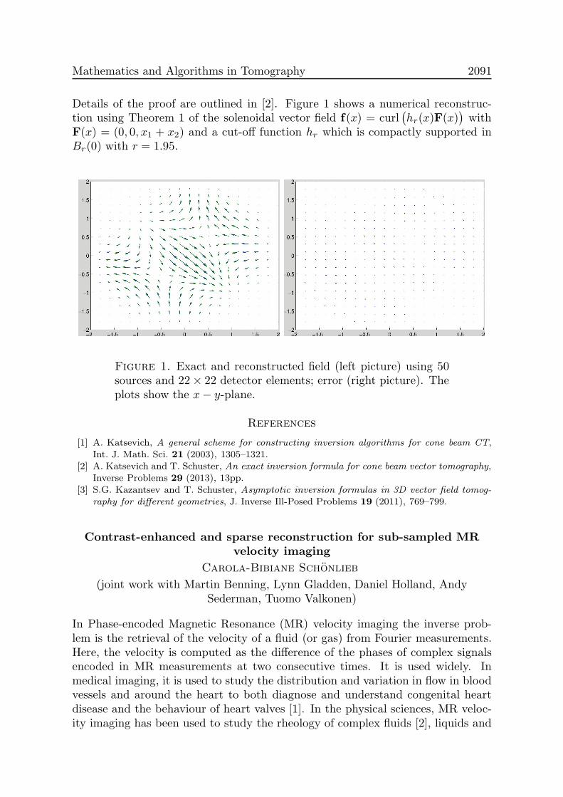
Mathematics and Algorithms in Tomography 2091
Details of the proof are outlined in [2]. Figure 1 shows a numerical reconstruc-tion using Theorem 1 of the solenoidal vector field f(x) = curl
(hr(x)F(x)
)with
F(x) = (0, 0, x1 + x2) and a cut-off function hr which is compactly supported inBr(0) with r = 1.95.
Figure 1. Exact and reconstructed field (left picture) using 50sources and 22× 22 detector elements; error (right picture). Theplots show the x− y-plane.
References
[1] A. Katsevich, A general scheme for constructing inversion algorithms for cone beam CT,Int. J. Math. Sci. 21 (2003), 1305–1321.
[2] A. Katsevich and T. Schuster, An exact inversion formula for cone beam vector tomography,Inverse Problems 29 (2013), 13pp.
[3] S.G. Kazantsev and T. Schuster, Asymptotic inversion formulas in 3D vector field tomog-raphy for different geometries, J. Inverse Ill-Posed Problems 19 (2011), 769–799.
Contrast-enhanced and sparse reconstruction for sub-sampled MR
velocity imaging
Carola-Bibiane Schonlieb
(joint work with Martin Benning, Lynn Gladden, Daniel Holland, AndySederman, Tuomo Valkonen)
In Phase-encoded Magnetic Resonance (MR) velocity imaging the inverse prob-lem is the retrieval of the velocity of a fluid (or gas) from Fourier measurements.Here, the velocity is computed as the difference of the phases of complex signalsencoded in MR measurements at two consecutive times. It is used widely. Inmedical imaging, it is used to study the distribution and variation in flow in bloodvessels and around the heart to both diagnose and understand congenital heartdisease and the behaviour of heart valves [1]. In the physical sciences, MR veloc-ity imaging has been used to study the rheology of complex fluids [2], liquids and

2092 Oberwolfach Report 37/2014
gases flowing through packed beds [3, 4, 5], granular flows [6, 7] and multiphaseturbulence [8]. The main advantage of MR for studying flow is that it is possibleto non-invasively image systems without the use of a tracer. However, a majordrawback of the technique, in both medical and non-medical applications, is theacquisition time of the measurement. In the medical field, long acquisition times(∼min) necessitate breath hold or triggered acquisition techniques that, althoughimpressive, are susceptible to artefacts and may be impractical in certain cases. Innon-medical applications, long acquisition times require very stable systems andcan prohibit the study of certain features, e.g. fine vortices in turbulent flow. Toovercome these limitations many studies have explored methods to increase thetemporal resolution of velocity-encoded imaging (e.g. [9, 10, 11]). These ultra-fast(¡ 1 s imaging time) techniques have all been demonstrated to provide a substan-tial improvement in the temporal resolution. However, despite these advances,each has limitations in terms of the systems that can be studied and the trade-offbetween spatial and temporal resolution. In this talk we discuss two variationalregularisation approaches which can both improve upon the spatial resolution ofreconstructions from sub-sampled k-space data. Both methods are based on thetheory of compressed sensing, exploiting prior knowledge of the signal or the veloc-ity in terms of appropriate variational regularisation techniques. The first methodis discussed in [12]. It constitutes the solution of the linear inverse problem ofreconstructing a complex signal from its MR measurements by variational regu-larisation, and computing the velocity as the difference of the phases of two soreconstructed signals. We are particularly interested in regularisers that correctlytreat both smooth and geometric features of the image. These features are com-mon to velocity imaging, where the flow field will be smooth but interfaces betweenthe fluid and surrounding material will be sharp, but are challenging to representsparsely. As an example we demonstrate the variational approaches on velocityimaging of water flowing through a packed bed of solid particles. We evaluateWavelet regularisation against Total Variation and the relatively recent secondorder Total Generalised Variation regularisation. We combine these regularisationschemes with a contrast enhancement approach called Bregman iteration. We ver-ify for a variety of sampling patterns that Morozovs discrepancy principle providesa good criterion for stopping the iterations. Therefore, given only the noise level,we present a robust guideline for setting up a variational reconstruction schemefor MR velocity imaging. The main disadvantage of this first approach is thatprior knowledge in terms of regularisation is not formulated for the quantity ofinterest, the velocity. This is suboptimal, especially since the amplitude and phaseof the complex image have very difference regularity properties, the former beingrelatively smooth while the latter being better approximated by a piecewise con-stant function. Therefore, we investigate a second approach where we attempt toreconstruct the desired velocity (the difference of the phases) directly, cf. also [13].This amounts to the solution of a nonlinear inverse problem in which the phase isnonlinearly (via the exponential function) related to the MR measurements. Weagain derive a variational regularisation model (this time the regularisation acts on
Mathematics and Algorithms in Tomography 2093
the velocity directly!) and employ for the solution of this – now nonlinear prob-lem – simultaneously linearisation and ADMM iteration. In each iteration thisresults in the solution of an unconstrained linear problem which we further breakdown to pure proximity operations by a surrogate approach. First experimentswith this approach promise improved reconstruction properties. The convergenceof the resulting iterative scheme still has to be analysed in more detail.
References
[1] P. Gatehouse, J. Keegan, L. Crowe, S. Masood, R. Mohiaddin, K.-F. Kreitner and D. Firmin,Applications of phase-contrast flow and velocity imaging in cardiovascular MRI, EuropeanRadiology 15 (2005), 2172–2184.
[2] P. Callaghan, Rheo-NMR: nuclear magnetic resonance and the rheology of complex fluids,Reports on Progress in Physics 62 (1999), 599–670.
[3] A. Sederman, M. Johns, P. Alexander and L. Gladden, Structure-flow correlations in packedbeds, Chemical engineering Science 53 (1998), 2117–2128.
[4] M. H. Sankey, D. J. Holland, L. F. Gladden and A. J. Sederman, Magnetic resonance velocityimaging of liquid and gas two-phase flow in packed beds, Journal of Magnetic Resonance196 (2009), 142–148.
[5] D. J. Holland, D. M. Malioutov, A. Blake, A. J. Sederman and L. F. Gladden, Reducingdata acquisition times in phase-encoded velocity imaging using compressed sensing, Journalof Magnetic Resonance 203 (2010), 236–246.
[6] E. Fukushima, Nuclear magnetic resonance as a tool to study flow, Annual Review of Fluid
Mechanics 31 (1999), 95–123.[7] D. J. Holland, L. F. Gladden, C. R. Muller, J. S. Dennis and A. J. Sederman, Spatially
resolved measurement of anisotropic granular temperature in gas-fluidized beds, PowderTechnology 182 (2008), 171–181.
[8] A. B. Tayler, D. J. Holland, A. J. Sederman and L. F. Gladden, Exploring the origins ofturbulence in multiphase flow using compressed sensing MRI, Physical Review Letters 108(2012), 264505.
[9] K. Kose, Instantaneous flow-distribution measurements of the equilibrium turbulent regionin a circular pipe using ultrafast NMR imaging, Physical Review A 44 (1991), 2495–2504.
[10] A. J. Sederman, M. D. Mantle, C. Buckley and L. F. Gladden, MRI technique for mea-surement of velocity vectors, acceleration, and autocorrelation functions in turbulent flow,Journal of Magnetic Resonance 166 (2004), 182–189.
[11] P. Galvosas and P. T. Callaghan, Fast magnetic resonance imaging and velocimetry forliquids under high flow rates, Journal of Magnetic Resonance 181 (2006), 119–125.
[12] M. Benning, L. Gladden, D. Holland, C. Schonlieb, T. Valkonen, Phase reconstructionfrom velocity-encoded MRI measurements – A survey of sparsity-promoting variational ap-proaches, Journal of Magnetic Resonance 238 (2014), 26–43.
[13] F. Zhao, D.C. Noll, J.F. Nielsen, J.A. Fessler, Separate magnitude and phase regularizationvia compressed sensing, Medical Imaging, IEEE Transactions on, 31(9), (2012), 1713–1723.
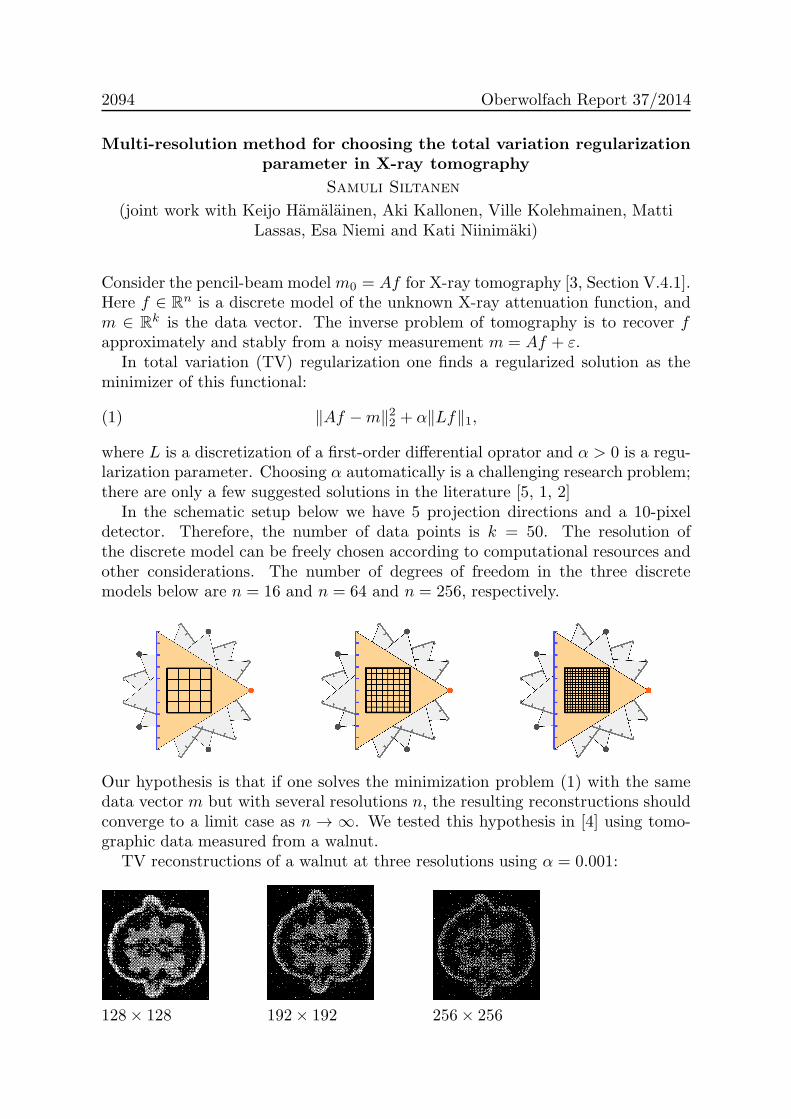
2094 Oberwolfach Report 37/2014
Multi-resolution method for choosing the total variation regularization
parameter in X-ray tomography
Samuli Siltanen
(joint work with Keijo Hamalainen, Aki Kallonen, Ville Kolehmainen, MattiLassas, Esa Niemi and Kati Niinimaki)
Consider the pencil-beam modelm0 = Af for X-ray tomography [3, Section V.4.1].Here f ∈ Rn is a discrete model of the unknown X-ray attenuation function, andm ∈ Rk is the data vector. The inverse problem of tomography is to recover fapproximately and stably from a noisy measurement m = Af + ε.
In total variation (TV) regularization one finds a regularized solution as theminimizer of this functional:
(1) ‖Af −m‖22 + α‖Lf‖1,
where L is a discretization of a first-order differential oprator and α > 0 is a regu-larization parameter. Choosing α automatically is a challenging research problem;there are only a few suggested solutions in the literature [5, 1, 2]
In the schematic setup below we have 5 projection directions and a 10-pixeldetector. Therefore, the number of data points is k = 50. The resolution ofthe discrete model can be freely chosen according to computational resources andother considerations. The number of degrees of freedom in the three discretemodels below are n = 16 and n = 64 and n = 256, respectively.
Our hypothesis is that if one solves the minimization problem (1) with the samedata vector m but with several resolutions n, the resulting reconstructions shouldconverge to a limit case as n → ∞. We tested this hypothesis in [4] using tomo-graphic data measured from a walnut.
TV reconstructions of a walnut at three resolutions using α = 0.001:
128× 128 192× 192 256× 256

Mathematics and Algorithms in Tomography 2095
TV reconstructions at three resolutions using a larger parameter α = 10:
128× 128 192× 192 256× 256As you can see in the above pictures, the smaller parameter leads to reconstruc-
tions that are unstable with respect to the resolution. On the other hand, usingthe larger parameter apparently gives converging reconstructions.
A systematic study of the same data with two noise levels suggests that itis reasonable to choose the smallest parameter α > 0 that leads to convergentreconstructions. Here is a table of TV norms of reconstructions (left: low noise,right: higher noise):
α 1282 1922 2562 1282 1922 2562
10−4 1.51 2.29 3.64 2.42 5.05 8.7110−3 1.51 2.29 3.46 2.43 5.05 8.5910−2 1.50 2.23 2.97 2.42 5.01 8.5910−1 1.43 1.85 1.93 2.37 4.83 8.16100 1.08 1.11 1.11 1.99 3.50 5.12101 0.78 0.78 0.77 0.86 0.86 0.88102 0.48 0.48 0.48 0.48 0.48 0.48103 0.12 0.12 0.12 0.12 0.12 0.12104 0.04 0.04 0.04 0.04 0.04 0.04105 0 0 0 0 0 0106 0 0 0 0 0 0
Careful study of the above numbers suggests choosing α = 1 for the low-noise caseand α = 10 for the high-noise case.
References
[1] K. Hamalainen, A. Kallonen, V. Kolehmainen, M. Lassas, K. Niinimaki, and S. Silta-
nen, Sparse tomography, SIAM Journal on Scientific Computing, 35 (2013), pp. B644–B665.[2] S. Kindermann, L. D. Mutimbu, and E. Resmerita, A numerical study of heuristic pa-
rameter choice rules for total variation regularization, Journal of Inverse and Ill-PosedProblems, 22 (2013), pp. 63–94.
[3] F. Natterer, The mathematics of computerized tomography, vol. 32 of SIAM Classics inApplied Mathematics, SIAM, 2001.
[4] K. Niinimaki, M. Lassas, K. Hamalainen, A. Kallonen, V. Kolehmainen, E. Niemi
and S. Siltanen, Multi-resolution parameter choice method for total variation regularizedtomography, arXiv:1407.2386 [math.NA]
[5] Y.-W. Wen and R. Chan, Parameter selection for total-variation-based image restorationusing discrepancy principle, Image Processing, IEEE Transactions on, 21 (2012), pp. 1770–1781.
2096 Oberwolfach Report 37/2014
Resolution-controlled conductivity discretization in electrical
impedance tomography
Andreas Rieder
(joint work with Robert Winkler)
In electrical impedance tomography (EIT) one wants to recover an isotropic con-ductivity distribution σ : Ω→ [c0,∞[, c0 > 0, in the interior of an object Ω ⊂ R2,e.g., a cross section of the human body. To this end, electric current is appliedon the boundary of the object through electrodes and the resulting voltages arerecorded at these electrodes as well.
The most accurate model for EIT to date is the complete electrode model (CEM)which we describe now in its variational formulation: Let Ω be a simply connectedLipschitz domain and let Ej ⊂ ∂Ω, j = 1, . . . , L, denote the distinct electrodeshaving positive surface measure. With this electrode configuration we associatethe electrode space
EL := spanχE1, . . . , χEL
∩ L2⋄(∂Ω) ⊂ L
2⋄(∂Ω)
where χEjis the indicator function of Ej and L2
⋄(∂Ω) is the space of L2-functionswith vanishing mean along the boundary. The forward problem now reads: Givenan electrode current I ∈ EL and a contact impedance z > 0, find a voltage potentialup ∈ H
1(Ω) and an electrode voltage U ∈ EL such that
a((up, U), (w,W )
)=
∫
∂Ω
I WdS for all (w,W ) ∈ H1(Ω)⊕ EL
where the bilinear form a on H1(Ω)⊕ EL is defined by
a((v, V ), (w,W )
):=
∫
Ω
σ∇v∇w dx+1
z
∫
∪jEj
(v − V )(w −W ) dS.
The above problem has a unique solution [5].The nonlinear forward operator describing CEM is the Neumann-to-Dirichlet
map R : D(R) ⊂ L∞(Ω)→ L(Ep), σ 7→ I 7→ U, where D(R) = σ ∈ L∞(Ω): σ ≥c0, that is, R(σ)I = U . Finally, we can phrase the inverse problem of EIT asthe reconstruction of σ from the knowledge of R(σ). Besides its illposedness thisinverse problem suffers from too few measurements. Indeed, since R(σ) can berepresented by a symmetric matrix of order L−1 = dim EL we only have L(L−1)/2independent measurements.
To bring the best out of the measurements a sensible discretization of the con-ductivity is required. Conductivity discretizations have been considered before,see, e.g., [1, 2, 4] to name a few, but an explicit resolution-based quantification ofthe discretization size for CEM across Ω is still an open task. In the remainder ofthis extended abstract we summarize our contribution to this task.
Motivated by Isaacson [3] we define the relative sensitivity for distinguishingthe conductivity σ from the reference or background conductivity σ by
λσ,σ :=‖R(σ)−R(σ)‖
‖R(σ)‖
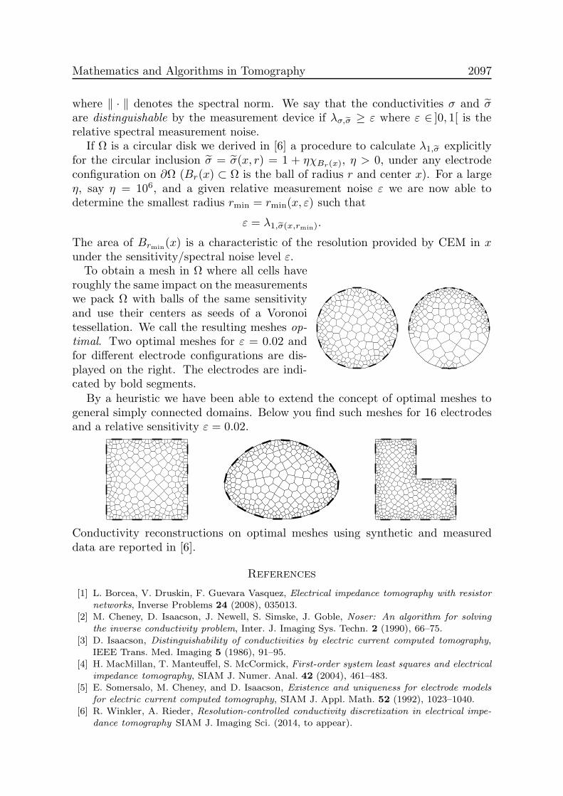
Mathematics and Algorithms in Tomography 2097
where ‖ · ‖ denotes the spectral norm. We say that the conductivities σ and σare distinguishable by the measurement device if λσ,σ ≥ ε where ε ∈ ]0, 1[ is therelative spectral measurement noise.
If Ω is a circular disk we derived in [6] a procedure to calculate λ1,σ explicitlyfor the circular inclusion σ = σ(x, r) = 1 + ηχBr(x), η > 0, under any electrodeconfiguration on ∂Ω (Br(x) ⊂ Ω is the ball of radius r and center x). For a largeη, say η = 106, and a given relative measurement noise ε we are now able todetermine the smallest radius rmin = rmin(x, ε) such that
ε = λ1,σ(x,rmin).
The area of Brmin(x) is a characteristic of the resolution provided by CEM in x
under the sensitivity/spectral noise level ε.To obtain a mesh in Ω where all cells have
roughly the same impact on the measurementswe pack Ω with balls of the same sensitivityand use their centers as seeds of a Voronoitessellation. We call the resulting meshes op-timal. Two optimal meshes for ε = 0.02 andfor different electrode configurations are dis-played on the right. The electrodes are indi-cated by bold segments.
By a heuristic we have been able to extend the concept of optimal meshes togeneral simply connected domains. Below you find such meshes for 16 electrodesand a relative sensitivity ε = 0.02.
Conductivity reconstructions on optimal meshes using synthetic and measureddata are reported in [6].
References
[1] L. Borcea, V. Druskin, F. Guevara Vasquez, Electrical impedance tomography with resistornetworks, Inverse Problems 24 (2008), 035013.
[2] M. Cheney, D. Isaacson, J. Newell, S. Simske, J. Goble, Noser: An algorithm for solvingthe inverse conductivity problem, Inter. J. Imaging Sys. Techn. 2 (1990), 66–75.
[3] D. Isaacson, Distinguishability of conductivities by electric current computed tomography,IEEE Trans. Med. Imaging 5 (1986), 91–95.
[4] H. MacMillan, T. Manteuffel, S. McCormick, First-order system least squares and electricalimpedance tomography, SIAM J. Numer. Anal. 42 (2004), 461–483.
[5] E. Somersalo, M. Cheney, and D. Isaacson, Existence and uniqueness for electrode modelsfor electric current computed tomography, SIAM J. Appl. Math. 52 (1992), 1023–1040.
[6] R. Winkler, A. Rieder, Resolution-controlled conductivity discretization in electrical impe-dance tomography SIAM J. Imaging Sci. (2014, to appear).

2098 Oberwolfach Report 37/2014
Time reversal and Cormack’s last paper
Victor Palamodov
1. Time reversal (in the spirit of M. Fink) [1]Let H ⊂ Rn be an open set (called cavity) in such that ∂H ⊂ Z, where Z be a
hypersurface (called mirror).An arbitrary function f supported by H is transmitted in a homogeneous
medium to the manifold R+ × Z, the result is filtered by an operator F actingin R+ × Z, time reversed and retransmitted and detected as a function g. A re-construction is given in the form Tf = pg for a known positive function p in Hdepending only on the geometry.
2. Theorem. The reconstruction is exact that is Tf = f if p is an arbitraryoscillatory polynomial and Z is the zero set of p with the density dZ = dx/dp andH is the hyperbolic cavity of p. The filtration operator F is a universal secondorder selfadjoint ”vertical” operator acting in R+ × Z [2],[3].
3. Oscillatory sets. Let p be a real polynomial in Rn of degree m with the zeroset Z. They are called oscillatory with respect to a cavity H ⊂ Rn\Z if p has msimple zeros in L for almost any line L ⊂ R that meets H. Hyperbolic cavity ofan oscillatory set Z any maximal connected cavity. There is only one boundedhyperbolic cavity, if Z is compact that is p is elliptic. Any hyperbolic cavity isconvex.
4. Examples. Any ellipsoid, elliptic paraboloid, elliptic and parabolic cylinder isoscillatory with only one hyperbolic cavity. Two sheet hyperboloid is oscillatorywith two hyperbolic cavities. If P = P (t, x) is a homogeneous polynomial inRn+1 that is hyperbolic with respect to t in the sense of I. Petrovsky, then thepolynomial p (x) = P (1, x) is oscillatory in Rn. For arbitrary n,m ≥ 2 the set ofoscillatory polynomials of n variables of degree m depends on several descrete andcontinual parameters.
5. Reconstruction from spherical means. This result is equivalent to some explicitFBP formulas for reconstruction of a function supported in H from data of sphericalintegrals for spheres with centers in Z [2],[3].
6. The last paper of Allan Cormack. Cormack proposed a method for determina-tion of distribution of a scattered material by filtering the scattered light on traveltimes. ”Suppose that waves travel in this space with a speed v and that the spacecontains a distribution of scattering material with a density f which is assumedto be smooth and either rapidly decreasing or of compact support... An impulsiveplane wave front with a normal ω reaches 0 at t = 0. As result of the well-known focusing property of paraboloids the scattering waves arriving at 0 at timet = 2p/v will all have originated on the paraboloid defined by r (1 + 〈ξ, ω〉) = 2p...”The mathematical problem is to reconstruct a function in a space from data of inte-grals over a family of confocal parabolas or confocal paraboloids. A reconstructionfor this acquisition geometry is given by an explicit FBP formula [2],[4].

Mathematics and Algorithms in Tomography 2099
References
[1] M. Fink and C. Prada, Acoustic time-reversal mirrors. Inverse Probl. 17 (2001), R1–R38.[2] V. P. Palamodov, A uniform reconstruction formula in integral geometry. Inverse Probl. 28
(2012) 065014.[3] V. P. Palamodov, Time reversal in photoacoustic tomography and levitation in a cavity.
arxiv: 1405.6283[4] V. P. Palamodov, A. Cormack last inversion formula and a FBP reconstruction. arxiv:
1407.8473
On artifacts in the limited data problem of spherical Radon Transform
Linh Nguyen
Let S be a smooth closed surface in Rn. We consider the following restrictedspherical Radon transform
R(f)(z, r) =
∫
S(z,r)
f(y) dσ(y), (z, r) ∈ S × R+.
Here, S(z, r) is the sphere of radius r centered at z. This transform appears in sev-eral imaging modalities, such as thermo/photo-acoustic tomography, ultrasoundtomography, SONAR, and Inverse Elasticity.
The problem of inverting R has attracted intensive studies in the last decade.A comprehensive reference list can be found in [4]. In this talk, we discuss themicrolocal analysis of a reconstruction formula with an emphasis on limited dataproblem.
Let us assume that S is the boundary of a convex domain Ω. We consider thefollowing operators:
P (h)(r) =
∫
R
∞∫
0
ei (τ2−r2)λ |λ|n−1 h(τ) dτ dλ.
and
B(g)(x) =1
2 πn
∫
S
g(z, |z − x|) 〈z − x, νz〉 dσ(z).
Here, νz is the outward normal of S at z. Then, if f is supported inside Ω,
B P R(f)(x) = f(x) +K(f)(x), for all x ∈ Ω,
where K is a pseudo-differential operator of order −1 (see [3, 1, 2, 4]). Moreover,K ≡ 0 if S is a sphere or an ellipse/ellipsoid (see [3, 1, 2]).
Let Γ be a proper subset of S with smooth boundary. Assume that we onlyknow R(f)(z, r) for z ∈ Γ. That is, we only have limited data. Up to now, thereis no closed form formula to find f from the limited data. In order to reconstructthe visible singularities of f , the following formula has been proposed
T (f)(x) := BΓ P R(f)(x),

2100 Oberwolfach Report 37/2014
where
BΓ(h)(x) =1
2 πn
∫
Γ
g(z, |z − x|) 〈z − x, νz〉 dσ(z).
Then, T (f) reconstructs all the visible singularities of f with the correct order.However, it also creates artifacts by rotating each (so-called) boundary singularityaround the corresponding boundary point of Γ ⊂ S. These artifacts are 1
2 -ordersmoother than the (original) boundary singularity. Detailed results can be foundin [5, 6].
Similar results for the case that Γ does not have smooth boundary can be foundin [5].
References
[1] M. Haltmeier, Inversion of circular means and the wave equation on convex planar domain,Computers & Mathematics with Applications 65 (3) (2013), 1025–1036.
[2] M. Haltmeier, Universal Inversion Formulas for Recovering a Function from SphericalMeans, SIAM Journal on Mathematical Analysis 46 (1) (2014), 214–232.
[3] F. Natterer, Photo-acoustic inversion in convex domains, Inverse Problems and Imaging 6(2012), 315–320.
[4] L.V Nguyen, On a reconstruction formula for spherical Radon transform: a microlocalanalytic point of view, Analysis and Mathematical Physics 4 (3) (2014), 199–220.
[5] L.V Nguyen, On Artifacts in Limited Data Spherical Radon Transform I: Flat ObservationSurfaces. arXiv preprint at arXiv:1407.4496 .
[6] L. Barannyk, J. Frikel, and L.V Nguyen, On Artifacts in Limited Data Spherical RadonTransform: Curved Observation Surfaces. Preprint.
PET imaging of freely moving mice via image registration
Frank Wubbeling
(joint work with Xiaoyi Jiang, Dirk Mannweiler, Julian Rasch, Klaus Schafers,and Sonke Schmid)
Positron Emission Tomography (PET) is an excellent tool for viewing the metab-olism of a live organism. Basically, a radioactive tracer is injected which accumu-lates for example at tumor cells. The emitted photons are detected, yielding theinformation that a decay took place on a line of response. In the limit of numberof photons going to infinity, the Radon transform of the distribution function ofthe tracer is measured on a grid, and standard Radon inversion techniques couldbe used [7]. However, since radiation and acquisition time are limited, in practicethese measurements are heavily corrupted by Poisson noise, which is taken intoaccount by the selection of appropriate statistical reconstruction algorithms [10].
So acquisition time is a crucial parameter for image quality. It is easily around15 minutes. Therefore, in small animal imaging e.g. mice are typically anaesthe-tized before studies are done. This prevents the application of PET as a quanti-tative method to analyze organ function that are affected by anesthesia (see eg.[1]), in particular brain activity. Thus, PET imaging of conscious, preferably even
Mathematics and Algorithms in Tomography 2101
freely moving, animals is highly desirable and currently being tried using dedicatedinstruments, see e.g. [5], [9], [4].
We present an alternative that does not employ specialized scanners, and whichwas tested with the QuadHIDAC wire chamber scanner. It is based on an algo-rithmical, mathematical approach, and demonstrates the value of the integrationof image analysis tools into reconstuction algorithms. We give a purely techni-cal description of what is done, the exact choices for mathematical modeling andimplementation can be found in the cited literature. The procedure is
(1) Take a normal PET scan of a freely moving mouse (it is in a cage).(2) Determine the motion of the mouse during the scan.(3) Perform a motion corrected, EM-based reconstruction.
For (1), an appropriate cage was built, equipped with four optical cameraswhich are used for mouse localization and motion detection, employing featurepoint algorithms. For the reconstruction part, the algorithms implemented inEMrecon [3] were used.
Optical Tracking provides only surface information. Since for PET reconstruc-tion we also need the interior motion, it has to be estimated, resulting in unsatis-factory accuracy.
To deal with this, we propose to complement the video with additional infor-mation delivered by volume preserving registration algorithms, like they are usedin human PET motion correction [2].
Observation of mice in the cage during the PET acquisition shows that in about40 percent of the time, the mice are not moving at all. These static phases rangefrom around 5 to 30 seconds. In order to derive information about interior motion,the following algorithm is applied.
(1) Using the video tapes, extract scenes without motion, meaning extractscenes that change by less than a certain threshold in an appropriate norm.
(2) From the low–SNR data acquired in these short scenes, reconstruct pre-liminary reconstructions. Note that due to the SNR, these will hardly bequantitative. EMTV–type algorithms are used for this [8].
(3) Use image registration of the low quality images to derive motion of theinterior of the mouse, VAMPIRE [2] and FAIR [6] were employed.
(4) Use the motion information to reconstruct a quantitative image from alldata acquired [3].
As a conclusion, the algorithm generally delivers quantitative results providedthe mice are not running around too erratically. However, it turns out that thebrain, which is the actual target, is extremely difficult to image, so that here theoutcome is still unclear. Currently, the algorithm is in pre–clinical testing.
References
[1] M. Desai et al., Mapping brain networks in awake mice using combined optical neural controland fMRI, J Neurophysiol. 2011 Mar;105(3):1393-405.
2102 Oberwolfach Report 37/2014
[2] Gigengack F, Ruthotto L, Burger M, Wolters CH, Jiang X, Schafers K, Motion correctionin dual gated cardiac PET using mass-preserving image registration, IEEE Transactions onMedical Imaging (2012), 31(3): 698–712
[3] Kosters T, Schafers K, Wubbeling F, EMRecon: an expectation maximization based im-age reconstruction framework for emission tomography data (2011), Proceedings of IEEEMedical Imaging Conference, Valencia
[4] Kyme A, Meikle S, Baldock C, Fulton R (2012), Refraction-compensated motion trackingof unrestrained small animals in positron emission tomography, Medical Image Analysis16:1317–1328.
[5] Mizuma H et al. (2010) Establishment of in vivo brain imaging method in conscious miceJ Nucl Med 51:1068-1075.
[6] J. Modersitzki, FAIR: Flexible Algorithms for Image Registration Philadelphia: SIAM,2009.
[7] Natterer F, Wubbeling F, Mathematical Methods in Image Reconstruction, SIAM 2001.[8] Sawatzky, Alex; Brune, Christoph; Wubbeling, Frank; Kosters, Thomas; Schafers, K.;
Burger, M. Accurate EM-TV algorithm in PET with low SNR, Nuclear Science Sympo-sium Conference Record, 2008. NSS ’08. IEEE , vol., no., pp.5133,5137, 19-25 Oct. 2008
[9] Schulz D et al. Simultaneous assessment of rodent behavior and neurochemistry using aminiature positron emission tomography, Nature Methods 2011 8(4):347-352.
[10] Shepp L., Vardi Y. Maximum likelihood reconstruction for emission tomography. MedicalImaging, IEEE Transactions on, 1982, 1(2):113:122.
A Nonlinear Variational Approach to Motion-Corrected
Reconstruction of Density Images
Sebastian Suhr
(joint work with Martin Burger, Jan Modersitzki)
Modelling and Analysis
In our setup, we will be concerned with reconstruction a sequence of probabilitydensities ρ0, . . . , ρN on Ω ⊂ Rd, typically d = 2, 3 such that
(1) ρk(x) = ρ0(yk(x))det(∇yk(x)),
with a reasonably smooth deformation field yk. The measurements fk are noisyversions of K(ρk), with a stationary forward operator K, e.g. a convolution influorescence microscopy or versions of the x-ray transform in PET and SPECT.
We are going to minimize a problem of the form
(2) J(ρ, y) =
N∑
k=0
(D(Kρk, fk) + αkRI(ρk) + βkRM (yk)) ,
subject to (1). Here D is the data fidelity between estimated and measured data,and RI respectively RM are regularization functionals on the image respectivelymotion (with nonnegative regularization parameters αk and βk).
Since we aim at reconstructing images with sharp edges we employ total varia-tion regularization ([1]) on the image, while we choose hyperelastic regularization([2]) for the motion field. In detail the hyperelastic energy is given by

Mathematics and Algorithms in Tomography 2103
(3) Shyper(y) =
∫
Ω
α1 len(∇y) + α2 surf(cof(∇y)) + α3 vol(det(∇y))dx ,
with the penalty functions
len(s) = ‖s− I‖2Fro , surf(s) =(‖s‖2Fro − 3
)2, vol(s) =
(s− 1)4
s2.
The three terms punish deviations from the identity and in volume, length andsurface. Thus non local diffeomorphic transformations lead to infinite energies.Unfortunately there are some non global injective transformations, which are lo-cally injective everywhere.
We turn our focus on the analysis of the presented model. If we follow the directmethod in the calculus of variations, there are two properties of the functional tobe prooved:
• Coercivity• Lower semi-comtinuity
While coercivity can be obtained from the chosen regularization functionals theproof of lower semi-continuity is challenging. For weakly convergent sequences
ρk ∗ ρ in BV yk y in H1
we need to proove at least weak convergence, i.e:
(4) ρk(yk) det(∇yk) ρ(y) det(∇y) in L1
For this we need a changes of variables, but unfortunately the transforamtiontheorem for integrals does not hold in general. Therefore we use a generalizedform, the area formula ([5])
(5)
∫
E
ρ(y) det(∇y)dx =
∫
Rn
ρ(x)Nf (x,E)dx
Ny is the Banach Indicatrix and defined by:
(6) Nf (x,E) := card(f−1(x) ∩ E)
The crucial question is whether we can control the Banach Indicatrix in L∞.By using results from degree theory for Sobolev mappings ([4]) we can deducethis from the boundary behaviour of the mapping: An orientation preserving H1
mapping is injevtive, iff it is injective on the boundary.The question whether we can establish a bound of the following type
(7) ‖Ny‖∞ ≤ C(RM (y),Ω)
remains open.
2104 Oberwolfach Report 37/2014
Numerical Aspects
Similar to [7] we choose an altermating minimization approach, to minimize adiscretized version of the functional. This leads to a two step algorithm:
(1) Reconstruction Step: Minimize with respect to ρ for fix y(2) Motion Step: Minimize with respect to y for fix ρ
The first step leads to a minimization problem of the following type:
minρ0
∑
i
D(Kρ0(y(ti))|det(Dyi)|, fi) + αJ(ρ0)
ρ ≥ 0
This can be solved via reconstruction algorithms incorporating motion infor-mation ([3], [1]).
The reconstruction step boils down to:
miny
n−1∑
i=1
D(Kρ0(yi)|det(Dyi)|, fi) +β
2
n−1∑
i=1
RM (yi)
(8)
As all summands are independent, we have to solve n−1 registration problems.Although the distance measure is defined on the detector domain, this can be donewith standard registration algorithms like [6].
While the implementation of both steps is well understood, the challenge liesin the enforcing of injective transformations. A simple way would be to chooseDirichlet boundary conditions with y|∂Ω = Id, but this might be too restrictive.Thus the question of a gereralized registration framework for injective transforma-tions arises.
References
[1] Christoph Brune, Alex Sawatzky, and Martin Burger. Bregman-EM-TV methods with ap-plication to optical nanoscopy. In Scale Space and Variational Methods in Computer Vision.Springer Berlin / Heidelberg, 2009.
[2] M. Burger, J. Modersitzki, and L. Ruthotto. A hyperelastic regularization energy for imageregistration. SIAM Journal on Scientific Computing, 35(1):B132–B148, 2013.
[3] Thomas Kosters et al. Combined AW-OSEM reconstruction and mass-preserving motioncorrection of PET data. In The 12th International Meeting on Fully Three-DimensionalImage Reconstruction in Radiology and Nuclear Medicine, 2013.
[4] M. Giaquinta, G. Modica, and J. Soucek. Remarks on the degree theory. Journal of Func-tional Analysis, 125(1):172 – 200, 1994.
[5] Piotr Haj lasz. Change of variables formula under minimal assumptions. Colloq. Math.,64(1):93–101, 1993.
[6] Jan Modersitzki. FAIR: Flexible Algorithms for Image Registration. SIAM, 2009.[7] B. A. Mair, David R. Gilland , Jing Sun. Estimation of images and nonrigid deformations
in gated emission ct. IEEE Transactions on Medical Imaging, 25:1130–1144, 2006.

Mathematics and Algorithms in Tomography 2105
On the V-line Radon transform and its applications in imaging
Gaik Ambartsoumian
(joint work with Rim Gouia-Zarrad, Sunghwan Moon)
Single scattering optical tomography uses light, transmitted and scattered throughan object, to determine the interior features of that object. If the object has mod-erate optical thickness it is reasonable to assume that the majority of photonsscatter once. Using collimated emitters and receivers one can measure the in-tensity of light scattered along various broken rays corresponding to the paths ofsuch photons. These measurements are then used to recover the spatially varyingcoefficients of light absorption and/or light scattering. The latter task is mathe-matically equivalent to the problem of inversion of a generalized Radon transformintegrating along V-shaped broken rays (see [2, 3, 5] and the references there).
Since the family of broken rays in 2D is 4-dimensional, the inversion problemdescribed above is overdetermined. Hence it is natural to consider the problem ofinversion from integrals of image function along a 2D subset of broken rays.
Definition 2. The V-line Radon transform (VRT) of function f(x, y) is the in-tegral
(1) Rf(p1, p2) =
∫
BR(p1,p2)
f ds,
of f along the broken ray BR(p1, p2) with respect to line measure ds.
There are many ways to restrict the 4D family of broken-rays to a 2D subset.Motivated by geometric setups of other tomographic modalities, convenience ofhardware implementation and symmetries simplifying the analysis, we considerbelow the cases of VRT in circular and rectangular geometries of data acquisition.
The left figure above describes the circular setup of VRT, where A(φ) corre-sponds to the location of the light source, the points Cj = C(φ, tj) correspondto the locations of (an array of) receivers, and Bj = B(φ, tj) are the scatteringpoints, where tj is the distance from the breaking point to the origin. In the caseof a fixed scattering angle α ∈ (0, π/2) we have proved the following statement.

2106 Oberwolfach Report 37/2014
Theorem 7. [1] If f(x, y) is a smooth function supported in the disc D(0, R),then f is uniquely determined by Rf(φ, t), φ ∈ [0, 2π], t ∈ [0, R].
The proof of the theorem also provides an exact reconstruction formula of ffrom Rf(φ, t) in this setup. Please see [1] for further details.
In the rectangular setup we consider broken rays with a fixed scattering angle2β symmetric with respect to y-axis (see the right-hand side figure above). Suchrays can be uniquely parameterized by the Cartesian coordinates (xv, yv) of theirvertices. In this case we have proved the following inversion result.
Theorem 8. [4] Let f(x, y) be a smooth function supported in D = (x, y) ∈ R2 |0 ≤ x ≤ xmax, 0 ≤ y ≤ ymax. For (xv, yv) ∈ R2 and fixed β ∈ (0, π2 ) denoteg(xv, yv) = Rf(xv, yv). Then
f(x, y) = −cosβ
2
[∂
∂yg(x, y) + tan2(β)
∫ ymax
y
∂2
∂x2g(x, t) dt
].
A natural generalization of the rectangular setup to 3D leads to consideration ofthe conical Radon transform (CRT). CRT integrates the image function of 3 vari-ables over a 3D family of circular cones with fixed opening angle symmetric to thez-axis. Parameterizing each cone by the coordinates of its vertex (xv, yv, zv) anddenoting the CRT g(xv, yv, zv) = Rf(xv, yv, zv), we prove the following statement.
Theorem 9. [4] An exact solution of the inversion problem for CRT is given by
fλ,µ(z) = C(β)
∫ z
zmax
J0 (u(z − x))
[d2
dx2+ u2
]2 ∫ x
zmax
gλ,µ(zv) dzv dx
where gλ,µ(zv) and fλ,µ(z) are the 2D Fourier transforms of the functionsg(xv, yv, zv) and f(x, y, z) with respect to the first two variables, C(β) =
cos2 β/(2π sinβ) and u = tanβ√λ2 + µ2.
The author thanks the organizers of the Oberwolfach workshop “Mathematicsand Algorithms in Tomography” for the invitation and opportunity to participatein such a great conference. He also expresses gratitude to the MathematischesForschungsinstitut Oberwolfach and US National Science Foundation for his travelsupport as a US Junior Oberwolfach Fellow. Part of this work was funded by NSFDMS-1109417 grant.
References
[1] G. Ambartsoumian and S. Moon, A series formula for inversion of the V-line Radon trans-form in a disc, Computers and Mathematics with Application, 66 (9), (2013), 1567–1572.
[2] L. Florescu, V. A. Markel and J. C. Schotland, Inversion formulas for the broken-ray Radontransform, Inverse Problems 27 (2011), 025002.
[3] L. Florescu, J. C. Schotland and V. A. Markel, Single scattering optical tomography, Phys.Rev. E 79 (2009), 036607.
[4] R. Gouia-Zarrad and G. Ambartsoumian, Exact inversion of the conical Radon transformwith a fixed opening angle, Inverse Problems 30 (2014), 045007.
[5] A. Katsevich and R. Krylov, Broken ray transform: inversion and a range condition, InverseProblems 29 (2013), 075008.

Mathematics and Algorithms in Tomography 2107
Approximate marginalization of uninteresting unknowns in inverse
problems
Ville Kolehmainen
(joint work with Jari P. Kaipio, Antti Nissinen)
In the Bayesian inverse problems framework, all unknown parameters are treatedas random variables and all uncertainties can be modeled systematically. Recently,the approximation error approach has been proposed for handling modeling errorsdue to unknown nuisance parameters and model reduction [1, 2, 3]. In this ap-proach, approximate marginalization of the modeling errors is carried out beforethe estimation of the interesting variables. In this talk, we describe the approx-imation error approach and present computational examples that are related tolocal X-ray tomography imaging and electrical impedance tomography.
References
[1] Kaipio, J. and Somersalo, E. (2007). Statistical inverse problems: discretization, modelreduction and inverse crimes. J Comput Appl Math, 198.
[2] Kolehmainen, V., Tarvainen, T., Arridge, S. R., and Kaipio, J. P. (2011). Marginalizationof uninteresting distributed parameters in inverse problems – application to optical tomog-raphy. Int. J. Uncertainty Quantification, 1(1), 1–17.
[3] Jari Kaipio and Ville Kolehmainen. Approximate marginalization over modelling errors anduncertainties in inverse problems. In Paul Damien, Petros Dellaportas, Nicholas G. Polsonand David A. Stephens, editors, Bayesian Theory and Applications. Oxford University Press(Oxford, UK), pages 644-672, (2013).
Cone beam transverse ray transform
David Finch
(joint work with Patcharee Wongsason)
(Preliminary Report)
The object discussed in this talk is the transverse ray transform of a compactlysupported vector field in Euclidean geometry. For a vector field f , point a, anddirection θ, the transverse ray transform of f at a in direction θ, denoted T f(a, θ)is given by
(1) T f(a, θ) =
∫ ∞
0
Pθf(a+ tθ) dt
where Pθ denotes orthogonal projection on the subspace perpendicular to θ. Thetransverse ray transform is complementary to the more frequently studied longitu-dinal or Doppler transform. The problem addressed is the recovery of a compactlysupported vector field in three dimensional Euclidean space, from the data of itstransverse ray transform for all points a lying in a space curve Γ and for all di-rections. Our arguments follow closely the work of Katsevich and Schuster, aspresented at this workshop by Prof. Dr. Schuster. Under the assumption that fis C2 supported in the unit ball, and that Γ is a Tuy curve of order three with

2108 Oberwolfach Report 37/2014
respect to the ball, we show that f may be recovered by an explicit formula. Theproof has three main steps. The first is to establish a Grangeat type formula,similar to that found by Kazantsev and Schuster for the Doppler transform, whichrelates the an operator applied to the tangential part of the Radon transform of f(taken componentwise) evaluated at (a · θ, θ) ∈ R × S2 to an operator applied tothe transverse ray transform at a. Then, as for Katsevich and Schuster, combiningthe results for the several sources lying on the plane containing a with normal θallows to solve for the derivative of the tangential part of the Radon transform.This is the same intermediate data obtained by Katsevich and Schuster, so theirmethod gives a formula to recover the solenoidal part of f . If f is written asf = ∇φ+ f s where φ has compact support in the ball and f s has zero divergence,then T∇φ = D∇φ, where D is the usual divergent beam x-ray transform. Anyof the various reconstruction formulas for the cone beam transform may then beemployed to recover ∇φ. Details will appear in a manuscript in preparation.
Acknowledgement
DF was partially supported by NSF grant DMS-100914. PW was partially sup-ported by a Royal Thai graduate fellowship.
References
[1] A. Katsevich and T. Schuster, An exact inversion formula for cone bean vector tomography,Inverse Problems 29 (2013), article id 065013.
[2] P. Wongsason, 3D cone beam resconstruction formulas for the transverse-ray transform withsource points on a curve, PhD thesis, Oregon State University, (2014).
π-line reconstruction formulas in tomography: numerical analysis of
view dependent derivatives
Adel Faridani
(joint work with Ryan Hass)
Let
(1) Df(y, θ) =
∫ ∞
0
f(y + tθ) dt
denote the divergent beam transform. We are concerned with the numerical anal-ysis of the view dependent derivative
(2)∂
∂qDf(y(q), θ)
∣∣∣∣q=s
that occurs in so-called π-line inversion formulas for fan-beam and 3D helicaltomography [1, 3, 4, 5, 8, 12].

Mathematics and Algorithms in Tomography 2109
For example, the derivative is present in the filtered-backprojection reconstruc-tion formula
(3) f(x) =1
2π2
∫
Iπ(x)
1
|x− y(s)|
∫ 2π
0
∂
∂qDf(y(q), θ(s, x, γ))
∣∣∣∣q=s
dγ
sin γds
derived in [4], as well as in the backprojection-filtration formulas of [12]. It isworth noting that even in the 2D case where very good algorithms are available,algorithms based on (3) can offer advantages in some situations, for example whenthe x-ray source comes very close to the object. Furthermore, in our numericalexperiments we found the convergence rate for smooth functions f to be the sameas for the standard filtered backprojection algorithm. However, careful implemen-tation of the derivative (2) has been found to be critical to achieve competitiveperformance of reconstruction algorithms. We present a detailed analysis for thewell-known 2D fan-beam case with curved detector array and circular source curve.In this geometry one measures
g(s, α) = Df(y(s), θ(s, α))
where y(s) = R(cos s, sin s), θ(s, α) = sin(α)eu(s) + cos(α)ev(s), with eu(s) =(− sin s, cos s), and ev(s) = −y(s)/|y(s)| = −(cos s, sin s). The view dependentderivative can now be expressed in terms of the detector coordinates (s, α) andreads
(4)d
dqDf(y(q), θ(s, α))
∣∣∣∣q=s
=∂g
∂s(s, α) +
∂g
∂α(s, α).
We determine the leading error terms for several discretization schemes for (2)that have been proposed in the literature. Discretization schemes were generallyclassified in two distinct groups, depending on wether they were derived directlyfrom (2) or from discretizing the right hand side of (4). For our analysis we use aunified framework by expressing all schemes in the second, chain rule based format.The detailed analysis can be found in our forthcoming paper [2]. Some of mainresults are as follows. In practice the sampling stepsize ∆s is usually chosen muchlarger than ∆α. This choice is supported by the 2D sampling conditions for thedivergent beam transform [7] and needs to be taken into account when discretizing(2). Indeed, our analysis shows that this is the main reason why the so-calleddirect scheme, a straightforward discretization of (2), does not give satisfactoryresults. The NPH scheme derived in [9] improved on the direct scheme but waslater found to have non-isotropic resolution [11]. Our error analysis identifiesthe responsible error term. The ingenious NHDLH scheme [10] remedied thisdeficiency and set a new standard. Alternative and simpler improvements on theNPH scheme were the FHS [1] and the K [6] schemes. Our determination of theleading error terms for each scheme shows that the FHS scheme has the fewesterror terms which are shared by most of the other schemes, each of which also hasadditional terms. Nevertheless, in our numerical experiments for this geometrythe FHS, NHDLH, and K scheme give very comparable results. This is also truefor numerical experiments for flat detectors and/or elliptical source curves as long
2110 Oberwolfach Report 37/2014
as the detector array is aligned perpendicular to the source position y(s). Onthe other hand, our experi ments confirmed the findings in [10] that the NHDLHscheme gives clearly superior results in the particular case of an elliptical sourcecurve and detector array aligned parallel to d
dsy(s). The reason for this is subjectof our ongoing research.
References
[1] A. Faridani, R. Hass, and D.C. Solmon, D C, Numerical and theoretical explorations inhelical and fan-beam tomography, Journal of Physics: Conference Series 124 (2008), 012024.
[2] A. Faridani and R. Hass, On numerical analysis of view dependent derivatives in computedtomography (2014), submitted. Preprint available online athttp://people.oregonstate.edu/~faridana/preprints/preprints.html
[3] R. Hass and A.Faridani, Regions of backprojection and comet tail artifacts for π-line recon-struction formulas in tomography, SIAM J. Imaging Sci. 5 (2012), 1159–1184.
[4] A. Katsevich, Theoretically exact filtered backprojection-type inversion algorithm for spiralCT, SIAM J. Appl. Math. 62 (2002), 2012–2026.
[5] A. Katsevich, An improved exact filtered backprojection algorithm for spiral computed to-mography, Advances in Applied Mathematics 32 (2004), 681–697.
[6] A. Katsevich, A note on computing the derivative at a constant direction, Phys. Med. Biol.56 (2011), N53–N61.
[7] F. Natterer, Sampling in fan-beam tomography, SIAM J. Appl. Math. 53 (1993), 358–380.[8] F. Noo, M. Defrise, R. Clackdoyle, and H. Kudo, Image reconstruction from fan-beam
projections on less than a short scan, Phys. Med. Biol., 47 (2002), 2525–2546.[9] F. Noo, J. Pack, and D. Heuscher, Exact helical reconstruction using native cone-beam
geometries, Phys.Med. Biol. 48 (2003), 3787–3818.[10] F. Noo, S. Hoppe, F. Dennerlein, G. Lauritsch, and J. Hornegger, A new scheme for view-
dependent data differentiation in fan-beam and cone-beam computed tomography , Phys.Med. Biol. 52 (2007), 5393–5414.
[11] A. A. Zamyatin, K. Taguchi, and M. D. Silver, Practical Hybrid Convolution Algorithm forHelical CT Reconstruction, IEEE Trans. Nucl. Sci. 53 (2006), 167–174.
[12] Y. Zou and X. C. Pan, An extended data function and its generalized backprojection forimage reconstruction in helical cone-beam CT, Phys. Med. and Biol. 49 (2004), N383–N387.
Quantum walks with discrete time
F. Alberto Grunbaum
I will describe similarities and differences between classical random walks andquantum walks, their unitary counterparts. In particular they share a (properlyinterpreted) version of the renewal equation, and yet the importance of interferenceeffects in the quantum case produces very strikingly different results. Some ofthese have intriguing topological interpretations. This is part of joint work withL.Velazquez, R. Werner, A. Werner, J. Bourgain and J. Wilkening. A couple ofjoint papers have appeared in the last two years in CMP.
Reporter: Bernadette Hahn
Mathematics and Algorithms in Tomography 2111
Participants
Prof. Dr. Gaik Ambartsoumian
Department of MathematicsUniversity of Texas at ArlingtonP. O. Box 19408Arlington, TX 76019-0408UNITED STATES
Prof. Dr. Simon R. Arridge
Department of Computer ScienceUniversity College LondonGower StreetLondon WC1E 6BTUNITED KINGDOM
Prof. Dr. K. Joost Batenburg
Centrum Wiskunde & Informatica(CWI)Scientific Computing GroupScience Park 1231090 GB AmsterdamNETHERLANDS
Prof. Dr. Jan Boman
Matematiska InstitutionenStockholms Universitet10691 StockholmSWEDEN
Prof. Dr. Martin Burger
Institut fur Numerische undAngewandte MathematikUniversitat MunsterEinsteinstr. 6248149 MunsterGERMANY
Prof. Dr. Rolf Clackdoyle
Laboratoire Hubert CurienCNRS UMR 5516Campus Pole Opt. et Vision - Bat. F18, rue Prof. Benoit Lauras42000 St. EtienneFRANCE
Prof. Dr. Michel Defrise
Department of Nuclear MedicineVrije Universiteit BrusselUZ BrusselLaarbeeklaan 1011090 Jette (Brussels)BELGIUM
Prof. Dr. Laurent Desbat
TIMC - IMAGFaculte de MedicineUniversite de Grenoble38706 La Tronche CedexFRANCE
Dr. Oliver Dorn
School of MathematicsThe University of ManchesterOxford RoadManchester M13 9PLUNITED KINGDOM
Prof. Dr. Adel Faridani
Department of MathematicsOregon State UniversityKidder Hall 368Corvallis, OR 97331-4605UNITED STATES
Prof. Dr. David V. Finch
Department of MathematicsOregon State UniversityKidder Hall 368Corvallis, OR 97331-4605UNITED STATES
Dr. Jurgen Frikel
Institute of Computational BiologyHelmholtz Zentrum Munchen85764 NeuherbergGERMANY

2112 Oberwolfach Report 37/2014
Prof. Dr. F. Alberto Grunbaum
Department of MathematicsUniversity of CaliforniaBerkeley CA 94720-3840UNITED STATES
Dr. Bernadette Hahn
FR 6.1 - MathematikUniversitat des SaarlandesPostfach 15 11 5066041 SaarbruckenGERMANY
Prof. Dr. Per Christian Hansen
DTU ComputeSection for Scientific ComputingTechnical University of DenmarkBldg. 3032800 LyngbyDENMARK
Prof. Dr. Ming Jiang
Beijing International Center forMathematical Research (BICMR)Peking UniversityBeijing 100 871CHINA
Prof. Dr. Alexander Katsevich
Department of MathematicsUniversity of Central FloridaOrlando, FL 32816-1364UNITED STATES
Dr. Holger Kohr
Department of MathematicsKTH10044 StockholmSWEDEN
Prof. Dr. Ville Kolehmainen
Inverse Problems GroupDepartment of Applied PhysicsUniversity of Eastern FinlandYliopistonranta 1EP.O. Box 162770211 KuopioFINLAND
Prof. Dr. Leonid Kunyansky
Department of MathematicsUniversity of Arizona617 N. Santa RitaTucson AZ 85721-0089UNITED STATES
Dr. Aref Lakhal
Institut fur Angewandte MathematikUniversitat des SaarlandesPostfach 15115066041 SaarbruckenGERMANY
Prof. Dr. Armin Lechleiter
Zentrum fur TechnomathematikFB 3, Universitat BremenPostfach 330 44028334 BremenGERMANY
Prof. Dr. Alfred K. Louis
FR 6.1 - MathematikUniversitat des Saarlandes66041 SaarbruckenGERMANY
Dr. Linh Nguyen
Department of MathematicsUniversity of Idaho875 Perimeter Drive MSMoscow ID 83844UNITED STATES

Mathematics and Algorithms in Tomography 2113
Dr. Clifford Nolan
Department of Mathematics & StatisticsUniversity of LimerickLimerickIRELAND
Dr. Steven Oeckl
Fraunhofer EZRTFlugplatzstr. 7590768 FurthGERMANY
Dr. Ozan Oktem
Department of MathematicsKTH10044 StockholmSWEDEN
Prof. Dr. Victor P. Palamodov
School of Mathematical SciencesTel Aviv UniversityRamat AvivTel Aviv 69978ISRAEL
Dr. Sarah Patch
Department of PhysicsUniversity of Wisconsin-MilwaukeePO Box 413Milwaukee, WI 53201UNITED STATES
Prof. Dr. Eric Todd Quinto
Department of MathematicsTufts University503 Boston Ave.Medford, MA 02155UNITED STATES
Prof. Dr. Ronny Ramlau
Industrial Mathematics InstituteJohannes Kepler UniversityAltenbergerstr. 694040 LinzAUSTRIA
Prof. Dr. Andreas Rieder
Karlsruher Institut f. Technologie (KIT)Inst. f. Angew. & NumerischeMathematik76131 KarlsruheGERMANY
Dr. Gael Rigaud
Fachrichtung MathematikUniversitat des SaarlandesPostfach 15115066041 SaarbruckenGERMANY
Alex Sawatzky
Institute for Computational and AppliedMathematics - Imaging WorkgroupUniversitat MunsterEinsteinstr. 6248149 MunsterGERMANY
Prof. Dr. Otmar Scherzer
Computational Science CenterUniversitat WienNordbergstrasse 151090 WienAUSTRIA
Prof. Dr. Carola-Bibiane
Schoenlieb
Department of Applied Mathematics andTheoretical Physics (DAMTP)Centre for Mathematical SciencesWilberforce RoadCambridge CB3 OWAUNITED KINGDOM
Tobias Schon
Fraunhofer EZRTFlugplatzstr. 7590768 FurthGERMANY

2114 Oberwolfach Report 37/2014
Prof. Dr. John C. Schotland
Department of MathematicsUniversity of MichiganEast HallAnn Arbor, MI 48109-1109UNITED STATES
Prof. Dr. Thomas Schuster
Fachrichtung 6.1 - MathematikUniversitat des SaarlandesPostfach 15115066041 SaarbruckenGERMANY
Prof. Dr. Vladimir A.
Sharafutdinov
Novosibirsk State UniversityDepartment of Mathematics &MechanicsPirogova 2Novosibirsk 630 090RUSSIAN FEDERATION
Prof. Dr. Samuli Siltanen
Department of Mathematics & StatisticsUniversity of HelsinkiP.O. Box 6800014 University of HelsinkiFINLAND
Sebastian Suhr
Fachbereich MathematikUniversitat Munster48149 MunsterGERMANY
Prof. Dr. Gunther A. Uhlmann
Department of MathematicsUniversity of WashingtonPadelford HallBox 354350Seattle, WA 98195-4350UNITED STATES
Dr. Frank Wubbeling
Institut fur Numerische undAngewandte MathematikUniversitat MunsterEinsteinstr. 6248149 MunsterGERMANY