mathematics methods - tqa.tas.gov.au · pdf filemathematics methods ... plan activities and...

© Copyright for part(s) of this document may be held by organisations other than TASC Page 0 of 33 Version 1 Accredited for use from 1 January 2017

COURSE DOCUMENT

MATHEMATICS METHODS

COURSE CODE: MTM415117

LEVEL 4 / SIZE VALUE = 15

Version 1

Accredited for use from 1 January 2017

Mathematics Methods – Level 4 Page 1 of 33 Version 1 Accredited for use from 1 January 2017

MATHEMATICS METHODS

Rationale Mathematics is the study of order, relation and pattern. From its origins in counting and measuring it has evolved in highly sophisticated and elegant ways to become the language now used to describe much of the modern world. Mathematics is also concerned with collecting, analysing, modelling and interpreting data in order to investigate and understand real-world phenomena and solve problems in context. Mathematics provides a framework for thinking and a means of communication that is powerful, logical, concise and precise. It impacts upon the daily life of people everywhere and helps them to understand the world in which they live and work. Mathematics Methods Level 4 provides the study of algebra, functions, differential and integral calculus, probability and statistics. These are necessary prerequisites for the study of Mathematics Specialised Level 4 and as a foundation for tertiary studies in disciplines in which mathematics and statistics have important roles, including engineering, the sciences, commerce and economics, health and social sciences.

Aims Mathematics Methods Level 4 aims to develop learners’: understanding of concepts and techniques and problem solving

ability in the areas of algebra, function study, differential and integral calculus, probability and statistics

reasoning skills in mathematical contexts and in interpreting mathematical information

capacity to communicate in a concise and systematic manner using mathematical language.

MTM415117 Level 4 / Size Value = 15

Contents

Rationale 1 Aims 1 Learning Outcomes 2 Access 2 Pathways 2 Resources 2 Course Size and Complexity 3 Course Description 3 Course Requirements 3 Course Content 4 Assessment 8 Quality Assurance Processes 8 External Assessment Requirements 8 Criteria 9 Standards 10 Qualifications Available 18 Award Requirements 18 Course Evaluation 18 Course Developer 18 Expectations Defined by National Standards in Content Statements Developed by ACARA 19 Accreditation 25 Version History 25 Appendices 26


Learning Outcomes On successful completion of this course, learners will be able to:

understand the concepts and techniques in algebra, graphs, function study, differential and integral calculus, probability and statistics

solve problems using algebra, graphs, function study, differential and integral calculus, probability and statistics

apply reasoning skills in the context of algebra, graphs, function study, differential and integral calculus, probability and statistics

interpret and evaluate mathematical information and ascertain the reasonableness of solutions to problems

communicate their arguments and strategies when solving problems

plan activities and monitor and evaluate their progress

use strategies to organise and complete activities to organise and complete activities and meet deadlines in the context of mathematics

select and use appropriate tools, including computer technology, when solving mathematical problems. Additionally, learners will be given opportunities to demonstrate the following in line with the Australian Curriculum General Capabilities:

literacy skills

numeracy skills

information and communication technology skills

critical and creative thinking skills

ethical and intercultural understanding.

Access It is highly recommended that learners attempting this course will have successfully completed either of the courses, Mathematics Methods – Foundation Level 3 or the AC Mathematics 10A subject with some additional studies in introductory calculus. Assumed knowledge and skills are contained in both of these courses and will be drawn upon in the development of key knowledge and skills in Mathematics Methods.

Pathways Mathematics Methods Level 4 is designed for learners whose future pathways may involve mathematics and statistics and their applications in a range of disciplines at the tertiary level, including engineering, the sciences, and other related technology fields, commerce and economics, health and social sciences. It is highly recommended as a foundation course for the study of Mathematics Specialised Level 4.

Resources Learners must have access to calculator algebraic system (CAS) graphics calculators and become proficient in their use. These calculators can be used in all aspects of this course in the development of concepts and as a tool for solving problems. Refer also to the current TASC Calculator Policy that applies to Level 3 and 4 courses, available at www.tasc.tas.gov.au/0021. The use of computer software is also recommended as an aid to students’ learning and mathematical development. A range of packages such as, but not limited to: Wolfram Mathematica, Microsoft Excel, Autograph, Efofex Stat, Graph and Draw are appropriate for this purpose.

http://www.tasc.tas.gov.au/0021


Course Size and Complexity This course has a complexity level of 4. In general, courses at this level provide theoretical and practical knowledge and skills for specialised and/or skilled work and/or further learning, requiring:

broad factual, technical and some theoretical knowledge of a specific area or a broad field of work and learning

a broad range of cognitive, technical and communication skills to select and apply a range of methods, tools, materials and information to: o complete routine and non-routine activities o provide and transmit solutions to a variety of predictable and sometimes unpredictable problems

application of knowledge and skills to demonstrate autonomy, judgement and limited responsibility in known or changing contexts and within established parameters.

This level 4 course has a size value of 15.

Course Description Mathematics Methods Level 4 extends the study of elementary functions of a single variable to include the study of combinations of these functions, algebra, differential and integral calculus, probability and statistics and their applications in a variety of theoretical and practical contexts.

Course Requirements This course is made up of areas of study. While each of these is , the order of delivery is not

prescribed.

Function study

Circular (trigonometric) functions

Differential calculus

Integral calculus

Probability and statistics. These areas of study relate to Assessment Criteria 4 – 8. Assessment Criteria 1 – 3 apply to all five areas of study. Whilst the areas of study may be addressed separately and in any order, much of the content is inter-related and a more integrated approach is recommended and encouraged. It is also recommended that, where possible, concepts be developed within a context of practical applications. Such an approach provides learners with mathematical experiences that are much richer than a collection of skills. Learners thereby have the opportunity to observe and make connections between related aspects of the course and the real world and to develop further some important abstract ideas.


Course Content

FUNCTION STUDY

Learners will develop their understanding of the behaviour of a number of different functions. This area of study will include:

understanding the concept of a function as a mapping between sets, and as a rule or a formula that defines one variable quantity in terms of another (FS1)

using function notation, domain and range (FS2)

understanding the concept of the graph of a function (FS3)

reviewing the binomial theorem for (𝑎𝑥 + 𝑏)𝑛 and its link to Pascal’s triangle (formal derivation and extended problems involving particular terms not included) (FS4)

graphing polynomial functions in factored form with linear factors, including repeated factors (FS5)

reviewing the factorisation of polynomials and their use in curve sketching and determining the nature of stationary points (FS6)

recognising features and drawing graphs of 𝑦 = 𝑥𝑛 for 𝑛 = −2, −1,1

2, 1, 2 and 3, including shape and behaviour

as x and x (FS7)

defining logarithms as indices: 𝑎𝑥 = 𝑏 is equivalent to 𝑥 = log𝑎 𝑏 i.e. 𝑎log𝑎 𝑏 = 𝑏 (FS8)

establishing and using the algebraic properties of logarithms (FS9)

recognising the inverse relationship between logarithms and exponentials: 𝑦 = 𝑎𝑥 is equivalent to 𝑥 = log𝑎 𝑦 (FS10)

solving equations involving indices using logarithms (FS11)

recognising the qualitative features of the graphs of 𝑦 = 𝑎𝑥 and 𝑦 = log𝑎 𝑥 (𝑎 = 2, 𝑒 and 10) including domain,

range and, where relevant, asymptotes (FS12)

solving simple equations involving simple exponential and logarithmic functions algebraically and graphically (FS13)

defining the natural logarithm ln 𝑥 = log𝑒 𝑥 (FS14)

recognising and using the inverse relationship of the functions 𝑦 = 𝑒𝑥 and 𝑦 = ln 𝑥 (FS15)

understanding transformations (reflections, dilations and translations) from 𝑦 = 𝑓(𝑥) to 𝑦 = 𝐴𝑓[𝑛(𝑥 + ℎ)] + 𝑘,

where A, n, h and k ∈ R, A, n 0 (FS16)

using the functions articulated above to model practical situations (this does not include regression analysis) (FS17)

using the composition of functions where f composition g is defined by 𝑓(𝑔(𝑥)), given ran domg f (the notation

f g may be used, but is not required) (FS18)

solving equations of the form 𝑓(𝑥) = 𝑔(𝑥) over a specified interval, where f and g are functions of the styles specified above (using algebraic and calculator techniques where appropriate) (FS19)

sketching and interpreting polynomial, power, exponential and logarithmic functions, including simple transformations and combinations of these functions, including simple piecewise (hybrid) functions (FS20)

recognising the distinction between a function and a relation, including an informal consideration of one-to-one and many-to-one functions and the conditions for existence of an inverse function (FS21)

finding inverses of functions, including conditions for the existence of an inverse function, including exponential, logarithmic and power functions such as:

2( ) lnx bay a x b y c y ae c y a x b c

x b

(FS22)

finding the graphs of inverses derived from graphs of original functions. (FS23)


CIRCULAR (TRIGONOMETRIC) FUNCTIONS

Learners will develop their understanding of a range of circular (trigonometric) functions. This area of study will include:

using the angular measurements definition of radians and its relationship with degree measure (CTF1)

reviewing the trigonometrical relationships involving the unit circle: o the definition of sine, cosine and tangent (CTF2.1)

o the special relationships 𝑠𝑖𝑛2𝑥 + 𝑐𝑜𝑠2𝑥 = 1 (Pythagorean identity) and −1 ≤ 𝑠𝑖𝑛𝑥 ≤ 1, −1 ≤ 𝑐𝑜𝑠𝑥 ≤ 1 (CTF2.2)

o the identity sin

tancos

xx

x (CTF2.3)

o the special values; e.g. sin(0) = 0, cos(𝜋) = −1 (CTF2.4)

o the symmetry properties, such as sin(𝜋 ± 𝑥), cos(𝜋 ± 𝑥), sin(2𝜋 ± 𝑥) , cos(2𝜋 ± 𝑥)

tan(𝜋 ± 𝑥), tan(2𝜋 ± 𝑥) , sin (𝜋

2± 𝑥) , cos (

𝜋

2± 𝑥) , tan (

𝜋

2± 𝑥) (CTF2.5)

recognising the exact values for sine, cosine and tangent for: 𝜋

6,

𝜋

4,

𝜋

3,

𝜋

2 and integer multiples of these (CTF3)

recognising the graphs of 𝑦 = sin 𝑥 , 𝑦 = cos 𝑥 and 𝑦 = tan 𝑥 on extended domains (CTF4)

examining the effect of transformations of circular functions to:

𝑦 = 𝑎 sin(𝑏𝑥 + 𝑐) + 𝑑, 𝑦 = 𝑎 cos(𝑏𝑥 + 𝑐) + 𝑑, 𝑦 = 𝑎 tan(𝑏𝑥 + 𝑐) + 𝑑 (CTF5)

using inverse trigonometric functions to enable the solution of trigonometric equations of the form:

sin(𝑎𝑥 + 𝑏) = 𝑐, cos(𝑎𝑥 + 𝑏) = 𝑐, tan(𝑎𝑥 + 𝑏) = 𝑐

and also of the form sin(𝑎𝑥 + 𝑏) = 𝑘 cos(𝑎𝑥 + 𝑏) giving answers specific to a given domain (CTF6)

using the functions articulated in this section to model practical situations (this does not include regression analysis). (CTF7)

CALCULUS

Learners will study the graphical treatment of limits and differentiability of functions of a single real variable, and the differentiation and integration of these functions. This area of study will include: Differential Calculus:

reviewing the differences between the average rate of change and an instantaneous rate of change (CAL1)

reviewing the concept of a limit and the evaluation of a limit e.g. lim𝑥→𝑎

𝑓(𝑥) = 𝑝 (CAL2)

applying the first principles approach, 𝑓′(𝑥) = limℎ→0

𝑓(𝑥+ℎ)−𝑓(𝑥)

ℎ to determine the gradient functions of

2 3( ) ,f x x x

and other simple quadratic and cubic functions (CAL3)

determining the derivatives of for n Q, e and , , log , sin , cos tann x

ex x x x x and linear combinations of these

functions (formal derivation not examined) (CAL4)

determining the derivatives of ( )

( ) ( ), ( ) ( ),( )

f xf x g x f x g x

g x , and ( ( ))f g x where 𝑓 and 𝑔 are polynomial

functions, exponential, circular, logarithmic or power functions and transformations or simple transformations of these functions, or are simple manipulations of these (CAL5)

consideration of the differentiability of functions (CAL6)

finding the slope of a tangent and the equations of the tangent and normal to a curve at a point (CAL7)

determining instantaneous rates of changes (CAL8)

deducing the graph of the derivative function, including its domain, from the graph of a function (CAL9)


studying applications of differentiation to graphs and identifying the key features of graphs:

o identifying intervals over which a function is constant (stationary), strictly increasing or strictly decreasing (CAL10.1)

o identifying local maximums / minimums / stationary points of inflections over an interval (learners can choose to

use any methods as appropriate; the ‘change of sign of the first derivative’ test, the graph of the derivative, or the

second derivative test, to justify these) (CAL10.2)

o distinguishing between a local maximum / minimum and an end point maximum / minimum (CAL10.3)

studying the applications of differentiation to solving problems (CAL11)

constructing and interpreting position-time graphs, with velocity as the slope of the tangent. (CAL12)

Integral Calculus:

understanding anti-differentiation, recognising that ( ) ( )F x f x implies that ( ) ( )f x dx F x c (CAL13)

determining anti-derivatives (indefinite integrals) of polynomial functions and functions of the form ( )f ax b where

f is nx , for , , sin( ), cos( )xn Q e x x and combinations of these (CAL14)

informally considering the definite integral as a limiting value of a sum involving quantities such as area under a curve

and the informal treatment of the fundamental theorem of calculus, ∫ 𝑓(𝑥)𝑑𝑥 = 𝐹(𝑏) − 𝐹(𝑎)𝑏

𝑎 (CAL15)

applying integration to problems involving a function given a boundary condition, calculating the area of a region under a curve and simple cases of areas between curves (CAL16)

determining the equation of a function given its gradient or the equation of a tangent at a point on the curve (CAL17)

investigating applications of integration, including displacement as the integral of velocity. (CAL18)

PROBABILITY AND STATISTICS

Learners will study scenarios involving discrete and continuous random variables, their representation using tables, probability functions specified by rule and defining parameters (as appropriate); the calculation and interpretation of central measures and measure and spread; and statistical inference for sample proportions.

This area of study will include:

understanding the concept of a random variable as a real function defined on a sample space, studying examples of discrete and continuous random variables (PS1)

investigating discrete random variables: o specifying probability distributions for discrete random variables using graphs, tables and probability mass functions

(PS2.1)

o calculating, interpreting and using the expected value (E), the mean ( ), variance ( 2 ) of a discrete random

variable with and without technology (PS2.2) o recognising the property that, for many random variables, approximately 95 per cent of the distribution is within

two standard deviations of the mean (PS2.3) o using discrete random variables and associated probabilities to solve practical problems (PS2.4)

applying the binomial distribution to the number of successes in a fixed number, n, of Bernoulli trials with probability p of success: o examining the effect of the parameters n and p on the graph of the probability function (PS3.1)

o calculating probabilities P(X = r) = (nr

) pr(1 − p)n−r associated with the binomial distribution with

parameters n and p; noting the mean np and variance np(1 − p) of a binomial distribution (PS3.2) o using binomial distributions and associated probabilities to model data and solve practical problems (PS3.3)


studying the normal distribution: o identifying contexts such as naturally occurring variation that are suitable for modelling by normal random

variables (PS4.1)

o recognising features of the graph of the probability density function of the normal distribution with mean 𝜇

and standard deviation 𝜎 and the use of the standard normal distribution (PS4.2)

o using technology to calculate the mean , variance 2 and standard deviation from given continuous data

(PS4.3) o using the ‘68-95-99% approximation’ rule, to determine the proportions of a population within 1, 2 or 3 standard

deviations of the mean (PS4.4) o calculating probabilities and quantiles associated with a given normal distribution using technology, and use

these to solve practical problems (PS4.5) o calculating mean and standard deviation of a normal distribution given proportion information (PS4.6) o recognising features of the standard normal distribution N (0, 1). (PS4.7)

studying statistical inference, including the definition and distribution of a sample proportions, simulations and confidence intervals: o understanding the distinction between a population parameter and a sample statistic, using a sample statistic to

estimate the population parameter (PS5.1)

o using the concept of the sample proportion ˆX

pn

as a random variable whose value varies between samples,

where X is a binomial random variable which is associated with the number of items that have a particular characteristic and n is the sample size (PS5.2)

o using the approximate normality of the distribution of p̂ for large samples and, for such a situation, the mean p ,

(the population proportion) and standard deviation 1( )

p

p p

n

(PS5.3)

o from a large sample, determining an approximate confidence interval

1 1ˆ ˆ ˆ ˆ( ) ( )ˆ ˆ,

p p p pp z p z

n n

for a population proportion where z is the appropriate quantile for the

standard normal distribution. Whilst the 95% confidence interval is a particular example of such an interval where

1 96.z is mainly used, some consideration should be made to other confidence intervals, including the 90% and

the 99%. (The terms ‘standard error’ or ‘approximate margin of error’ may be used but are not required). (PS5.4)


Assessment Criterion-based assessment is a form of outcomes assessment that identifies the extent of learner achievement at an appropriate end-point of study. Although assessment – as part of the learning program – is continuous, much of it is formative, and is done to help learners identify what they need to do to attain the maximum benefit from their study of the course. Therefore, assessment for summative reporting to TASC will focus on what both teacher and learner understand to reflect end-point achievement. The standard of achievement each learner attains on each criterion is recorded as a rating ‘A’, ‘B’, or ‘C’, according to the outcomes specified in the standards section of the course. A ‘t’ notation must be used where a learner demonstrates any achievement against a criterion less than the standard specified for the ‘C’ rating. A ‘z’ notation is to be used where a learner provides no evidence of achievement at all. Providers offering this course must participate in quality assurance processes specified by TASC to ensure provider validity and comparability of standards across all awards. Further information on quality assurance processes, as well as on assessment, is available on the TASC website at http://www.tasc.tas.gov.au. Internal assessment of all criteria will be made by the provider. Providers will report the learner’s rating for each criterion to TASC. TASC will supervise the external assessment of designated criteria which will be indicated by an asterisk (*). The ratings obtained from the external assessments will be used in addition to internal ratings from the provider to determine the final award.

The following processes will be facilitated by TASC to ensure there is:

a match between the standards of achievement specified in the course and the skills and knowledge demonstrated by learners

community confidence in the integrity and meaning of the qualification.

– TASC gives course providers feedback about any systematic differences in the relationship of their internal

and external assessments and, where appropriate, seeks further evidence through audit and requires corrective action in the future.

The external assessment for this course will comprise:

a three hour written examination assessing criteria: 4, 5, 6, 7 and 8. For further information see the current external assessment specifications and guidelines for this course available on the TASC website.

http://www.tqa.tas.gov.au/


The assessment for Mathematics Methods Level 4 will be based on the degree to which the learner can: 1. communicate mathematical ideas and information 2. apply mathematical reasoning and strategy in problem solving situations 3. use resources and organisational strategies 4. *understand polynomial, hyperbolic, exponential and logarithmic functions 5. *understand circular functions 6. *use differential calculus in the study of functions 7. *use integral calculus in the study of functions 8. *understand binomial and normal probability distributions and statistical inference.

* denotes criteria that are both internally and externally assessed


CRITERION 1: COMMUNICATE MATHEMATICAL IDEAS AND INFORMATION

RATING ‘C’ RATING ‘B’ RATING ‘A’

The learner:

The learner: The learner:

presents work that shows some of the mathematical processes that have been followed between question and answer

presents work that conveys a line of reasoning that has been followed between question and answer

presents work that conveys a logical line of reasoning that has been followed between question and answer

uses mathematical conventions and symbols. There may be some errors or omissions in doing so

uses mathematical conventions and symbols correctly

uses mathematical conventions and symbols correctly

presents work with the final answer apparent

presents work with the final answer clearly identified

presents work with the final answer clearly identified, and articulated in terms of the question as required

uses correct units and includes them in an answer for routine problems

uses correct units and includes them in an answer for routine problems

uses correct units and includes them in an answer for routine and non-routine problems

presents tables, graphs and diagrams that include some suitable annotations

presents detailed tables, graphs and diagrams that convey clear meaning

presents detailed tables, graphs and diagrams that convey accurate meaning and precise information

adds a diagram to a solution as directed

adds a diagram to illustrate a solution

adds a detailed diagram to illustrate and explain a solution

works to an appropriate degree of accuracy as directed.

determines and works to an appropriate degree of accuracy.

ensures an appropriate degree of accuracy is maintained and communicated throughout a problem.


CRITERION 2: APPLY MATHEMATICAL REASONING AND STRATEGY IN PROBLEM SOLVING SITUATIONS


The learner:


identifies an appropriate strategy to solve routine problems

selects and applies an appropriate strategy to solve routine and simple non-routine problems

selects and applies an appropriate strategy, where several may exist, to solve routine and non-routine problems

describes solutions to routine problems

interprets solutions to routine and simple non-routine problems

interprets solutions to routine and non-routine problems

describes the appropriateness of the results of calculations

describes the reasonableness of results and solutions to routine problems

explains the reasonableness of results and solutions to routine problems and non- routine problems

identifies limitations of simple models

identifies and describes limitations of simple models

identifies and describes limitations of simple models

uses available technological aids to solve routine problems.

chooses to use available technological aids when appropriate to solve routine problems

uses available technological aids in familiar and unfamiliar contexts

explores calculator techniques in familiar contexts

explores calculator techniques in familiar and unfamiliar contexts

constructs and solves problems derived from routine scenarios.

constructs and solves problems derived from routine and non-routine scenarios.


CRITERION 3: USE RESOURCES AND ORGANISATIONAL STRATEGIES


The learner:


uses planning tools, with prompting, to achieve objectives within proposed times

uses planning tools to achieve objectives within proposed times

uses planning tools and strategies to achieve and manage activities within proposed times

divides a task into sub-tasks as directed

divides a task into sub-tasks divides a task into appropriate sub-tasks

uses given strategies and formulae to successfully complete routine problems

selects from a range of strategies and formulae to successfully complete routine problems

selects strategies and formulae to successfully complete routine and non- routine problems

monitors progress towards meeting goals

plans timelines and monitors progress towards meeting goals

plans timelines and monitors and analyses progress towards meeting goals, making adjustments as required

addresses most elements of required tasks

addresses the elements of required tasks

addresses all of the required elements of a task with a high degree of accuracy

uses prescribed strategies to adjust goals and plans where necessary.

plans future actions, adjusting goals and plans where necessary.

plans future actions, effectively adjusting goals and plans where necessary.


CRITERION 4: *UNDERSTAND POLYNOMIAL, HYPERBOLIC, EXPONENTIAL AND LOGARITHMIC FUNCTIONS


The learner:

In addition to the standards for a C rating, the learner:

In addition to the standards for a C and a B rating, the learner:

can graph functions which involve a single transformation

can graph functions which may involve multiple transformations when presented in standard form

can graph functions which may involve multiple transformations, sophisticated algebra (e.g. use of log laws), and functions presented in an unfamiliar form

can recognise and determine the equation of a graph of a function which has undergone a single transformation

can recognise and determine the equation of a graph of a function which has undergone multiple transformations

can recognise and determine the equation of a graph of a function which has undergone more complex transformations

understands the difference between a relation and a function

can use the graph of a function to determine whether or not an inverse function exists, giving reasons

can (using appropriate notation) restrict the domain of a function in order to allow the existence of an inverse function

can algebraically find the inverse of routine functions

can algebraically find the inverse of complex functions (for example: exponential and logarithmic functions)

distinguishes between: one-to-one and many-to one and many-to-many relations

can produce the graph of an inverse from the graph of a function

can identify the domain and the range given the graph of a function or a relation

explains the relationship between the domain and the range of a function and the domain and range of its inverse

can use the definition of logarithm to change between index and logarithmic statements

uses the definition of logarithm and the log laws to solve logarithmic equations

solves more complex logarithmic equations, including cases which involve the application of multiple log laws and cases where an algebraic substitution may be required

can apply log laws to simplify expressions

recognises when an answer is not feasible

determines simple composite functions.

determines more complex composite functions.

can establish the existence of a composite function by considering the domain and range of the component functions.


CRITERION 5: *UNDERSTAND CIRCULAR FUNCTIONS


The learner: In addition to the standards for a C rating, the learner:


can convert between degrees and radians

can use the CAST diagram to simplify expressions of the type:

sin (𝜋

2+ 𝜃), etc.

can use a suitable method to evaluate a second ratio from a given one.

E.g. Given that 𝑠𝑖𝑛𝑥 = −12

13 and

3

2x

, find 𝑐𝑜𝑠𝑥 and 𝑡𝑎𝑛𝑥

can recall exact values of trigonometric ratios for

30 2

6 4 2 2, , , , , ,

and

also recall exact values when these angles are expressed in degrees

can use the CAST diagram to evaluate a trig ratio of an angle

of greater than 2

expressing

the answer as an exact value.

E.g. Evaluate 𝑐𝑜𝑠7𝜋

6

can use the Pythagorean identity to evaluate a second ratio from a given one within the first quadrant. E.g. Given that

𝑠𝑖𝑛𝑥 =12

13 and 0 < 𝑥 <

𝜋

2

find 𝑡𝑎𝑛𝑥

can graph trigonometric functions which involve a single transformation. For example:

2 2

16

y x y x

y x y x

sin , sin

sin( ), sin

can graph trigonometric functions which involve multiple transformations but which are presented in the form:

sin ( )y a b x c d

Graphs of this type include functions where the horizontal

dilation factor is a multiple of .

E.g. 2 1siny x

can graph trigonometric functions which involve a multiple transformations which may be presented in an unfamiliar form. For example:

sin( )y a bx c d

Can identify endpoints and y intercept as exact values

can give the equation of a graph that has undergone a single transformation

can give the equation of a graph that has undergone multiple transformations

can use the inverse trig functions to identify the principal angle that has a given trig value. E.g.

Find x if 𝑠𝑖𝑛𝑥 = −1

2

can find specific solutions over a given domain to trig equations which are presented in standard

form. E.g. 𝑐𝑜𝑠2 (𝑥 +𝜋

3) =

1

2

can find specific solutions over a given domain to trig equations, presented in unfamiliar forms or which might involve a horizontal

dilation factor as a multiple of .

can find specific solutions over a given domain to simple trig equations which relate directly to the standard formula. Eg:

s𝑖𝑛𝑥 = −1

2 where 0 < 𝑥 < 2𝜋

can produce a graphical model of such an equation.


CRITERION 6: *USE DIFFERENTIAL CALCULUS IN THE STUDY OF FUNCTIONS


The learner:



can explain the concept of a limit and evaluate a simple limit

can evaluate limits that require initial simplification (e.g. factorisation)

can use the definition of derivative to differentiate a linear expression

can explain the definition of a derivative and how it relates to the gradient of a tangent to a curve

presents detailed working when using the definition of derivative and can use it on more complex examples

applies differentiation rules to differentiate expressions of the

type: , , ln , sin ,n xkx ke k x k x

cos , tank x k x and functions

that are the sum of each of these types. E.g. Differentiate:

45 3 xy x e

applies differentiation rules to differentiate products, quotients, rational functions and simple composite expressions

applies differentiation rules to differentiate complex expressions. Such cases include examples which involve multiple use of the composite rule and examples where several rules are used

finds the equation(s) of the tangent and/or normal to a curve given a point on the curve or the gradient for polynomial cases

finds the equation(s) of the tangent and/or normal to a curve given a point on the curve or the gradient for routine non polynomial cases

finds the equation(s) of the tangent and/or normal to a curve given a point on the curve or the gradient in cases where significant algebraic manipulation may be involved. Examples include use of log laws and evaluation of trigonometric exact values

uses the derivative to calculate an instantaneous rate of change in a practical example

articulates the difference between the average rate of change and the instantaneous rate of change and can calculate both in the context of a practical example

can choose the appropriate rate of change (average or instantaneous)

can deduce the graph of a derivative from the graph of a polynomial or other simple functions

can deduce the graph of a derivative from the graph of a more complex (possibly discontinuous) function

finds the stationary points of routine functions.

finds and justifies stationary points of routine functions and interprets the results.

finds and justifies stationary points of routine and non- routine functions and interprets the results.


CRITERION 7: *USE INTEGRAL CALCULUS IN THE STUDY OF FUNCTIONS


The learner:



determines the indefinite integral of a polynomial function in expanded form

the function of (𝑎𝑥 + 𝑏)𝑛 , where

n is a positive integer, and eax

integrates more complex functions which involve the direct application of a rule including;

𝑠𝑖𝑛(𝑎𝑥 + 𝑏) and 1

ax b

integrates functions which may require algebraic manipulation before applying a rule. Such examples include integration by recognition

calculates the area between the graph of a polynomial function and

the 𝑥-axis by evaluating the definite integral (in cases where

the graph does not cut the 𝑥-axis within the range of the integration)

calculates the area between the graph of a polynomial or a simple

exponential function and the 𝑥-axis by evaluating the definite integral (in cases where the graph

could cut the 𝑥-axis within the range of the integration)

calculates the area between the graph of more complex

functions and the 𝑥-axis by evaluating the definite integral. This could include, hyperbolic, trigonometric or logarithmic functions

evaluates the area between the graphs of two polynomial functions that do not intersect within the range of the integration

evaluates the area between the graphs of two polynomial functions with points of intersection that are easily determined

evaluates the area between the graphs of two more complex functions with two or more points of intersection that are easily determined

determines the distance travelled by an object moving in a straight line in one direction by integrating a simple polynomial velocity function in time

determines the distance travelled by an object moving in a straight line with one or two changes in direction by integrating a polynomial velocity function in time

integrates more complex functions and makes similar applications of integration to calculate net changes

can determine the equation of a polynomial function given its gradient and a point on the curve of the function. Such examples may involve the tangent at the contact point.

can determine the equation of a more complex function given its gradient and a point on the curve of the function.

can determine the equation of a function given an expression representing its gradient and a point on the curve of the function, in cases where sophisticated algebra such as logarithm laws or trigonometric exact values are required.


CRITERION 8: *UNDERSTAND BINOMIAL AND NORMAL PROABILTY DISTRUBTIONS AND STATISTICAL INFERENCE


The learner:



identifies and defines randomness, discrete and continuous variables

calculates the expected value (mean) for a discrete random variable

calculates the standard deviation and/or variance for a discrete random variable. can determine the 95% confidence interval for a given random variable

can solve problems involving finding unknown probabilities for a discrete random variable where the mean and variance is given

calculates (using technology) a binomial probability for a single outcome in routine cases

uses the formula

𝑃 = (nr

) pr(1 − p)n−r to

determine binomial probability for a single outcome in routine cases.

Calculates (using technology) a binomial probability for cumulative outcomes in routine cases

uses the formula

𝑃 = (nr

) pr(1 − p)n−r to

determine binomial probabilities for cumulative outcomes.

Calculates (using technology) a binomial probability for single and multiple outcomes where sophisticated modelling may be required

can draw the graph of a probability distribution for a discrete random variable

can draw the graph of a binomial distribution given values of x, n and p

can predict changes to the graph of a binomial distribution given changing values of n and p

can use technology to determine mean and standard deviation in a normal distribution.

Can use the ‘68-95-99% approximation’ rule

can use technology to determine probabilities in a normal distribution

can, given the population size, use technology to determine quantities in a normal distribution can, given a proportion, use inverse normal calculations to determine appropriate percentiles

can determine the mean and standard deviation of normally distributed data given proportion information. E.g. 10% of a population of animals has a mass < 1.2 kg, 20% has a mass > 3.8 kg. Find the mean and standard deviation

can calculate the mean and the standard (margin of) error of the sample proportion.

can construct the 95% confidence interval for a population proportion and can articulate their findings.

can construct confidence intervals for a population proportion and can articulate their findings. This may include the 90% and the 99% confidence intervals.


Mathematics Methods Level 4 (with the award of): EXCEPTIONAL ACHIEVEMENT HIGH ACHIEVEMENT COMMENDABLE ACHIEVEMENT SATISFACTORY ACHIEVEMENT PRELIMINARY ACHIEVEMENT

The final award will be determined by the Office of Tasmanian Assessment, Standards and Certification from 13 ratings (8 ratings from internal assessment and 5 ratings from external assessment). The minimum requirements for an award in Mathematics Methods Level 4 are as follows:

EXCEPTIONAL ACHIEVEMENT (EA) 11 ‘A’ ratings, 2 ‘B’ ratings (4 ‘A’ ratings and 1 ‘B’ rating from external assessment) HIGH ACHIEVEMENT (HA) 5 ‘A’ ratings, 5 ‘B’ ratings, 3 ‘C’ ratings (2 ‘A’ ratings, 2 ‘B’ ratings and 1 ‘C’ rating from external assessment) COMMENDABLE ACHIEVEMENT (CA) 7 ‘B’ ratings, 5 ‘C’ ratings (2 ‘B’ ratings and 2 ‘C’ ratings from external assessment) SATISFACTORY ACHIEVEMENT (SA) 11 ‘C’ ratings (3 ‘C’ ratings from external assessment) PRELIMINARY ACHIEVEMENT (PA) 6 ‘C’ ratings

A learner who otherwise achieves the ratings for a CA (Commendable Achievement) or SA (Satisfactory Achievement) award but who fails to show any evidence of achievement in one or more criteria (‘z’ notation) will be issued with a PA (Preliminary Achievement) award.

Course Evaluation The Department of Education’s Curriculum Services will develop and regularly revise the curriculum. This evaluation will be informed by the experience of the course’s implementation, delivery and assessment. In addition, stakeholders may request Curriculum Services to review a particular aspect of an accredited course. Requests for amendments to an accredited course will be forward by Curriculum Services to the Office of TASC for formal consideration. Such requests for amendment will be considered in terms of the likely improvements to the outcomes for learners, possible consequences for delivery and assessment of the course, and alignment with Australian Curriculum materials. A course is formally analysed prior to the expiry of its accreditation as part of the process to develop specifications to guide the development of any replacement course.

Course Developer The Department of Education acknowledges the significant leadership of Gary Anderson, John Short and Kim Scanlon in the development of this course.


Expectations Defined by National Standards in Content Statements Developed by ACARA The statements in this section, taken from documents endorsed by Education Ministers as the agreed and common base for course development, are to be used to define expectations for the meaning (nature, scope and level of demand) of relevant aspects of the sections in this document setting out course requirements, learning outcomes, the course content and standards in the assessment. For the content areas of Mathematics Methods, the proficiency strands – Understanding; Fluency; Problem Solving; and Reasoning – build on learners’ learning in F-10 Australian Curriculum: Mathematics. Each of these proficiencies is essential, and all are mutually reinforcing. They are still very much applicable and should be inherent in the five areas of study. Mathematical Methods Unit 1 – Topic 1: Functions and Graphs

examine examples of direct proportion and linearly related variables (ACMMM002)

recognise features of the graph of 𝑦 = 𝑚𝑥 + 𝑐 , including its linear nature, its intercepts and its slope or gradient (ACMMM003)

find the equation of a straight line given sufficient information; parallel and perpendicular lines (ACMMM004)

solve linear equations. (ACMMM005)

examine examples of quadratically related variables (ACMMM006)

recognise features of the graphs of 𝑦 = 𝑥2 , 𝑦 = 𝑎(𝑥 − 𝑏)2 + 𝑐, and 𝑦 = 𝑎(𝑥 − 𝑏)(𝑥 − 𝑐), including their parabolic nature, turning points, axes of symmetry and intercepts (ACMMM007)

solve quadratic equations using the quadratic formula and by completing the square (ACMMM008)

find the equation of a quadratic given sufficient information (ACMMM009)

find turning points and zeros of quadratics and understand the role of the discriminant (ACMMM010)

recognise features of the graph of the general quadratic 𝑦 = 𝑎𝑥2 + 𝑏𝑥 + 𝑐. (ACMMM011)

examine examples of inverse proportion (ACMMM012)

recognise features of the graphs of 𝑦 =1

𝑥 and 𝑦 =

𝑎

𝑥−𝑏 , including their hyperbolic shapes, and their asymptotes.

(ACMMM013)

recognise features of the graphs of 𝑦 = 𝑥𝑛 for 𝑛 ∈ 𝑵, 𝑛 = −1 and 𝑛 = ½ , including shape, and behaviour as 𝑥 →∞ and 𝑥 → −∞ (ACMMM014)

identify the coefficients and the degree of a polynomial (ACMMM015)

expand quadratic and cubic polynomials from factors (ACMMM016)

recognise features of the graphs of 𝑦 = 𝑥3 , 𝑦 = 𝑎(𝑥 − 𝑏)3 + 𝑐 and 𝑦 = 𝑘(𝑥 − 𝑎)(𝑥 − 𝑏)(𝑥 − 𝑐), including shape,

intercepts and behaviour as 𝑥 → ∞ and 𝑥 → −∞ (ACMMM017)

factorise cubic polynomials in cases where a linear factor is easily obtained (ACMMM018) solve cubic equations using technology, and algebraically in cases where a linear factor is easily obtained

(ACMMM019)


understand the concept of a function as a mapping between sets, and as a rule or a formula that defines one variable quantity in terms of another (ACMMM022)

use function notation, domain and range, independent and dependent variables (ACMMM023) understand the concept of the graph of a function (ACMMM024)

examine translations and the graphs of 𝑦 = 𝑓(𝑥) + 𝑎 and 𝑦 = 𝑓(𝑥 + 𝑏) (ACMMM025)

examine dilations and the graphs of 𝑦 = 𝑐𝑓(𝑥) and 𝑦 = 𝑓(𝑘𝑥) (ACMMM026)

recognise the distinction between functions and relations, and the vertical line test. (ACMMM027) Unit 1 – Topic 2: Trigonometric Functions

review sine, cosine and tangent as ratios of side lengths in right-angled triangles (ACMMM028)

understand the unit circle definition of cos 𝜃, sin 𝜃 and tan 𝜃 and periodicity using degrees (ACMMM029)

define and use radian measure and understand its relationship with degree measure. (ACMMM032)

understand the unit circle definition of cos θ, sin θ and tan θ and periodicity using radians (ACMMM034)

recognise the exact values of sin 𝜃, cos 𝜃 and tan 𝜃 at integer multiples of 𝜋

6 and

𝜋

4 (ACMMM035)

recognise the graphs of 𝑦 = sin 𝑥, 𝑦 = cos 𝑥 , and 𝑦 = tan 𝑥 on extended domains (ACMMM036)

examine amplitude changes and the graphs of 𝑦 = 𝑎 sin 𝑥 and 𝑦 = 𝑎 cos 𝑥 (ACMMM037)

examine period changes and the graphs of 𝑦 = sin 𝑏𝑥, 𝑦 = cos 𝑏𝑥 , and 𝑦 = tan 𝑏𝑥 (ACMMM038)

examine phase changes and the graphs of 𝑦 = sin(𝑥 + 𝑐), 𝑦 = cos(𝑥 + 𝑐) and 𝑦 = tan 𝑏𝑥 (ACMMM039)

𝑦 = tan (𝑥 + 𝑐) and the relationships sin (𝑥 +𝜋

2) = cos 𝑥 and cos (𝑥 −

𝜋

2) = sin 𝑥 (ACMMM040)

identify contexts suitable for modelling by trigonometric functions and use them to solve practical problems (ACMMM042)

solve equations involving trigonometric functions using technology, and algebraically in simple cases. (ACMMM043) Unit 1 – Topic 3: Counting and Probability

understand the notion of a combination as an unordered set of 𝑟 objects taken from a set of 𝑛 distinct objects (ACMMM044)

use the notation (𝑛𝑟

) and the formula (𝑛𝑟

) =𝑛!

𝑟!(𝑛−𝑟)! for the number of combinations of 𝑟 objects taken from a set

of 𝑛 distinct objects (ACMMM045)

expand (𝑥 + 𝑦)𝑛 for small positive integers 𝑛 (ACMMM046)

recognise the numbers (𝑛𝑟

) as binomial coefficients, (as coefficients in the expansion of (𝑥 + 𝑦)𝑛 (ACMMM047)

Unit 2 – Topic 1: Exponential Functions

review indices (including fractional indices) and the index laws (ACMMM061)

use radicals and convert to and from fractional indices (ACMMM062) understand and use scientific notation and significant figures. (ACMMM063)


establish and use the algebraic properties of exponential functions (ACMMM064)

recognise the qualitative features of the graph of 𝑦 = 𝑎𝑥 𝑎 > 0) including asymptotes, and of its translations ( 𝑦 =𝑎𝑥 + 𝑏 and 𝑦 = 𝑎𝑥+𝑐) (ACMMM065)

identify contexts suitable for modelling by exponential functions and use them to solve practical problems (ACMMM066)

solve equations involving exponential functions using technology, and algebraically in simple cases. (ACMMM067) Unit 2 – Topic 3: Introduction to Differential Calculus

interpret the difference quotient 𝑓(𝑥+ℎ)−𝑓(𝑥)

ℎ as the average rate of change of a function 𝑓 (ACMMM077)

use the Leibniz notation 𝛿𝑥 and 𝛿𝑦 for changes or increments in the variables 𝑥 and 𝑦 (ACMMM078)

use the notation 𝛿𝑦

𝛿𝑥 for the difference quotient


ℎ where 𝑦 = 𝑓(𝑥) (ACMMM079)

interpret the ratios 𝑓(𝑥+ℎ)−𝑓(𝑥)

ℎ and

𝛿𝑦

𝛿𝑥 as the slope or gradient of a chord or secant of the graph of 𝑦 = 𝑓(𝑥).

(ACMMM080)

examine the behaviour of the difference quotient 𝑓(𝑥+ℎ)−𝑓(𝑥)

ℎ as ℎ → 0 as an informal introduction to the concept

of a limit (ACMMM081)

define the derivative 𝑓′(𝑥) as limℎ→0


ℎ (ACMMM082)

use the Leibniz notation for the derivative: 𝑑𝑦

𝑑𝑥= lim

𝛿𝑥→0

𝛿𝑦

𝛿𝑥 and the correspondence

𝑑𝑦

𝑑𝑥= 𝑓′(𝑥) where 𝑦 = 𝑓(𝑥)

(ACMMM083)

interpret the derivative as the instantaneous rate of change (ACMMM084)

interpret the derivative as the slope or gradient of a tangent line of the graph of 𝑦 = 𝑓(𝑥). (ACMMM085)

estimate numerically the value of a derivative, for simple power functions (ACMMM086)

examine examples of variable rates of change of non-linear functions (ACMMM087)

establish the formula 𝑑

𝑑𝑥(𝑥𝑛) = 𝑛𝑥𝑛−1 for positive integers 𝑛 by expanding (𝑥 + ℎ)𝑛 or by factorising (𝑥 + ℎ)𝑛 −

𝑥𝑛. (ACMMM088)

understand the concept of the derivative as a function (ACMMM089)

recognise and use linearity properties of the derivative (ACMMM090) calculate derivatives of polynomials and other linear combinations of power functions. (ACMMM091)

find instantaneous rates of change (ACMMM092)

find the slope of a tangent and the equation of the tangent (ACMMM093) construct and interpret position-time graphs, with velocity as the slope of the tangent (ACMMM094)

sketch curves associated with simple polynomials; find stationary points, and local and global maxima and minima; and

examine behaviour as 𝑥 → ∞ and 𝑥 → −∞ (ACMMM095)

solve optimisation problems arising in a variety of contexts involving simple polynomials on finite interval domains. (ACMMM096)

calculate anti-derivatives of polynomial functions and apply to solving simple problems involving motion in a straight line. (ACMMM097)


Unit 3 – Topic 1: Further Differentiation and Applications

estimate the limit of 𝑎ℎ−1

ℎ as ℎ → 0 using technology, for various values of 𝑎 > 0 (ACMMM098)

recognise that e is the unique number a for which the above limit is 1 (ACMMM099)

establish and use the formula 𝑑

𝑑𝑥(𝑒𝑥) = 𝑒𝑥 (ACMMM100)

use exponential functions and their derivatives to solve practical problems. (ACMMM101)

establish the formulas 𝑑

𝑑𝑥(sin 𝑥) = cos 𝑥, and

𝑑

𝑑𝑥(cos 𝑥) = − sin 𝑥 by numerical estimations of the limits and

informal proofs based on geometric constructions (ACMMM102)

use trigonometric functions and their derivatives to solve practical problems. (ACMMM103)

understand and use the product and quotient rules (ACMMM104)

understand the notion of composition of functions and use the chain rule for determining the derivatives of composite functions (ACMMM105)

apply the product, quotient and chain rule to differentiate functions such as 𝑥𝑒𝑥 , tan 𝑥, 1

𝑥𝑛 , 𝑥 sin 𝑥, 𝑒− 𝑥 sin 𝑥 and

𝑓(𝑎𝑥 + 𝑏). (ACMMM106)

understand the concept of the second derivative as the rate of change of the first derivative function (ACMMM108)

recognise acceleration as the second derivative of position with respect to time (ACMMM109)

understand the concepts of concavity and points of inflection and their relationship with the second derivative (ACMMM110)

understand and use the second derivative test for finding local maxima and minima (ACMMM111)

sketch curves associated with simple polynomials; find stationary points, and local and global maxima and minima; and

examine behaviour as 𝑥 → ∞ and 𝑥 → −∞ (ACMMM095)

solve optimisation problems arising in a variety of contexts involving simple polynomials on finite interval domains. (ACMMM096)

Unit 3 – Topic 2: Integrals

recognise anti-differentiation as the reverse of differentiation (ACMMM114)

use the notation ∫ 𝑓(𝑥)𝑑𝑥 for anti-derivatives or indefinite integrals (ACMMM115)

establish and use the formula ∫ 𝑥𝑛𝑑𝑥 =1

𝑛+1𝑥𝑛+1 + 𝑐 for 𝑛 ≠ −1 (ACMMM116)

establish and use the formula ∫ 𝑒𝑥𝑑𝑥 = 𝑒𝑥 + 𝑐 (ACMMM117)

establish and use the formulas ∫ sin 𝑥 𝑑𝑥 = −cos 𝑥 + 𝑐 and ∫ cos 𝑥 𝑑𝑥 = sin 𝑥 + 𝑐 (ACMMM118)

recognise and use linearity of anti-differentiation (ACMMM119)

determine indefinite integrals of the form ∫ 𝑓(𝑎𝑥 + 𝑏)𝑑𝑥 (ACMMM120)

identify families of curves with the same derivative function (ACMMM121)

determine 𝑓(𝑥), given 𝑓′ (𝑥) and an initial condition 𝑓(𝑎) = 𝑏 (ACMMM122)

determine displacement given velocity in linear motion problems. (ACMMM123)


examine the area problem, and use sums of the form ∑ 𝑓(𝑥𝑖) 𝛿𝑥𝑖𝑖 to estimate the area under the curve 𝑦 = 𝑓(𝑥) (ACMMM124)

interpret the definite integral ∫ 𝑓(𝑥)𝑑𝑥 𝑏

𝑎 as area under the curve 𝑦 = 𝑓(𝑥) if 𝑓(𝑥) > 0 (ACMMM125)

recognise the definite integral ∫ 𝑓(𝑥)𝑑𝑥 𝑏

𝑎 as a limit of sums of the form ∑ 𝑓(𝑥𝑖) 𝛿𝑥𝑖𝑖 (ACMMM126)

interpret ∫ 𝑓(𝑥)𝑑𝑥 𝑏

𝑎 as a sum of signed areas (ACMMM127)

recognise and use the additivity and linearity of definite integrals. (ACMMM128)

understand the concept of the signed area function 𝐹(𝑥) = ∫ 𝑓(𝑡)𝑑𝑡𝑥

𝑎 ACMMM129)

understand and use the theorem: 𝐹′(𝑥) =𝑑

𝑑𝑥(∫ 𝑓(𝑡)𝑑𝑡

𝑥

𝑎) = 𝑓(𝑥), and illustrate its proof geometrically

(ACMMM130)

understand the formula ∫ 𝑓(𝑥)𝑑𝑥 = 𝐹(𝑏) − 𝐹(𝑎)𝑏

𝑎 and use it to calculate definite integrals. (ACMMM131)

calculate the area under a curve (ACMMM132) calculate the area between curves in simple cases (ACMMM134)

determine positions given values of velocity. (ACMMM135) Unit 3 – Topic 3: Discrete Random Variables

understand the concepts of a discrete random variable and its associated probability function, and their use in modelling data (ACMMM136)

use relative frequencies obtained from data to obtain point estimates of probabilities associated with a discrete random variable (ACMMM137)

recognise uniform discrete random variables and use them to model random phenomena with equally likely outcomes (ACMMM138)

examine simple examples of non-uniform discrete random variables (ACMMM139)

recognise the mean or expected value of a discrete random variable as a measurement of centre, and evaluate it in simple cases (ACMMM140)

recognise the variance and standard deviation of a discrete random variable as a measures of spread, and evaluate them in simple cases (ACMMM141)

use discrete random variables and associated probabilities to solve practical problems. (ACMMM142)

use a Bernoulli random variable as a model for two-outcome situations (ACMMM143) identify contexts suitable for modelling by Bernoulli random variables (ACMMM144)

recognise the mean 𝑝 and variance 𝑝(1 − 𝑝) of the Bernoulli distribution with parameter 𝑝 (ACMMM145)

use Bernoulli random variables and associated probabilities to model data and solve practical problems. (ACMMM146)

understand the concepts of Bernoulli trials and the concept of a binomial random variable as the number of

‘successes’ in 𝑛 independent Bernoulli trials, with the same probability of success 𝑝 in each trial (ACMMM147)

identify contexts suitable for modelling by binomial random variables (ACMMM148)

determine and use the probabilities P(X = r) = (nr

) pr(1 − p)n−r associated with the binomial distribution with

parameters n and p note the mean np and variance np(1 − p) of a binomial distribution (ACMMM149)

use binomial distributions and associated probabilities to solve practical problems (ACMMM150)


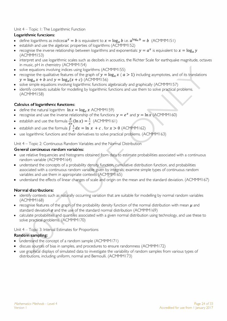
Unit 4 – Topic 1: The Logarithmic Function

define logarithms as indices:𝑎𝑥 = 𝑏 is equivalent to 𝑥 = log𝑎 𝑏 i.e. 𝑎log𝑎 𝑏 = 𝑏 (ACMMM151) establish and use the algebraic properties of logarithms (ACMMM152)

recognise the inverse relationship between logarithms and exponentials: 𝑦 = 𝑎𝑥 is equivalent to 𝑥 = log𝑎 𝑦 (ACMMM153)

interpret and use logarithmic scales such as decibels in acoustics, the Richter Scale for earthquake magnitude, octaves in music, pH in chemistry (ACMMM154)

solve equations involving indices using logarithms (ACMMM155)

recognise the qualitative features of the graph of 𝑦 = log𝑎 𝑥 ( 𝑎 > 1) including asymptotes, and of its translations

𝑦 = log𝑎 𝑥 + 𝑏 and 𝑦 = log𝑎(𝑥 + 𝑐) (ACMMM156)

solve simple equations involving logarithmic functions algebraically and graphically (ACMMM157)

identify contexts suitable for modelling by logarithmic functions and use them to solve practical problems. (ACMMM158)

define the natural logarithm ln 𝑥 = log𝑒 𝑥 ACMMM159)

recognise and use the inverse relationship of the functions 𝑦 = 𝑒𝑥 and 𝑦 = ln 𝑥 (ACMMM160)

establish and use the formula 𝑑

𝑑𝑥(ln 𝑥) =

1

𝑥 (ACMMM161)

establish and use the formula ∫1

𝑥𝑑𝑥 = ln 𝑥 + 𝑐 , for 𝑥 > 0 (ACMMM162)

use logarithmic functions and their derivatives to solve practical problems. (ACMMM163) Unit 4 – Topic 2: Continuous Random Variables and the Normal Distribution

use relative frequencies and histograms obtained from data to estimate probabilities associated with a continuous random variable (ACMMM164)

understand the concepts of a probability density function, cumulative distribution function, and probabilities associated with a continuous random variable given by integrals; examine simple types of continuous random variables and use them in appropriate contexts (ACMMM165)

understand the effects of linear changes of scale and origin on the mean and the standard deviation. (ACMMM167)

identify contexts such as naturally occurring variation that are suitable for modelling by normal random variables (ACMMM168)

recognise features of the graph of the probability density function of the normal distribution with mean μ and

standard deviation σ and the use of the standard normal distribution (ACMMM169)

calculate probabilities and quantiles associated with a given normal distribution using technology, and use these to solve practical problems. (ACMMM170)

Unit 4 – Topic 3: Interval Estimates for Proportions

understand the concept of a random sample (ACMMM171)

discuss sources of bias in samples, and procedures to ensure randomness (ACMMM172)

use graphical displays of simulated data to investigate the variability of random samples from various types of distributions, including uniform, normal and Bernoulli. (ACMMM173)


understand the concept of the sample proportion �̂� as a random variable whose value varies between samples, and

the formulas for the mean 𝑝 and standard deviation √(𝑝(1 − 𝑝)/𝑛 of the sample proportion �̂� (ACMMM174)

examine the approximate normality of the distribution of �̂� for large samples (ACMMM175)

simulate repeated random sampling, for a variety of values of p and a range of sample sizes, to illustrate the

distribution of �̂� and the approximate standard normality of 𝑝 −𝑝

√(𝑝(1−𝑝)/𝑛 where the closeness of the approximation

depends on both n and p. (ACMMM176)

the concept of an interval estimate for a parameter associated with a random variable (ACMMM177)

use the approximate confidence interval (�̂� − 𝑧 √(�̂�(1 − �̂�)/𝑛, �̂� + 𝑧 √(�̂�(1 − �̂�)/𝑛), as an interval estimate for

𝑝 , where 𝑧 is the appropriate quantile for the standard normal distribution (ACMMM178)

define the approximate margin of error 𝐸 = 𝑧 √(�̂�(1 − �̂�)/𝑛 and understand the trade-off between margin of error

and level of confidence (ACMMM179)

use simulation to illustrate variations in confidence intervals between samples and to show that most but not all

confidence intervals contain 𝑝 (ACMMM180)

Accreditation The accreditation period for this course is from 1 January 2017, with a decision regarding renewal of accreditation to be made within twelve (12) months and contingent on the outcomes of the Years 9-12 Review process.

Version History Version 1 – Accredited on 17 August 2016 for use from 1 January 2017. This course replaces MTM315114 Mathematics

Methods that expired on 31 December 2016.


Appendices

The algebraic properties of exponential functions are the index laws: 𝑎𝑥𝑎𝑦 = 𝑎𝑥+𝑦 , 𝑎−𝑥 =1

𝑎𝑥 , (𝑎𝑥)𝑦 = 𝑎𝑥𝑦 ,

𝑎0 = 1, where 𝑥, 𝑦 and 𝑎 are real.

The refers to ‘addition of intervals of integration’:

∫ 𝑓(𝑥)𝑑𝑥 + ∫ 𝑓(𝑥)𝑑𝑥 = ∫ 𝑓(𝑥)𝑑𝑥𝑐

𝑎

𝑐

𝑏

𝑏

𝑎

for any numbers 𝑎, 𝑏 and 𝑐 and any function 𝑓(𝑥).

The algebraic properties of exponential functions are the index laws: 𝑎𝑥𝑎𝑦 = 𝑎𝑥+𝑦 , 𝑎−𝑥 =1

𝑎𝑥 , (𝑎𝑥)𝑦 = 𝑎𝑥𝑦 ,

𝑎0 = 1 , for any real numbers 𝑥, 𝑦, and 𝑎, with 𝑎 > 0

The algebraic properties of logarithms are the rules: log𝑎(𝑥𝑦) = log𝑎 𝑥 + log𝑎 𝑦, log𝑎1

𝑥= − log𝑎 𝑥 , and log𝑎 1 = 0,

for any positive real numbers 𝑥, 𝑦 and 𝑎

An , or of a function 𝑓(𝑥) is a function 𝐹(𝑥) whose derivative is (𝑥) , i.e.

𝐹′(𝑥) = 𝑓(𝑥).

The process of solving for anti-derivatives is called .

Anti-derivatives are not unique. If 𝐹(𝑥) is an anti-derivative of 𝑓(𝑥), then so too is the function 𝐹(𝑥) + 𝑐 where 𝑐 is

any number. We write ∫ 𝑓(𝑥)𝑑𝑥 = 𝐹(𝑥) + 𝑐 to denote the set of all anti-derivatives of 𝑓(𝑥). The number 𝑐 is called

the For example, since 𝑑

𝑑𝑥(𝑥3) = 3𝑥2, we can write ∫ 3𝑥2 𝑑𝑥 = 𝑥3 + 𝑐

A straight line is an of the function y = 𝑓(𝑥) if graph of y = 𝑓(𝑥) gets arbitrarily close to the straight line.

An asymptote can be horizontal, vertical or oblique. For example, the line with equation 𝑥 =𝜋

2 is a vertical asymptote to

the graph of 𝑦 = tan 𝑥, and the line with equation 𝑦 = 0 is a horizontal asymptote to the graph of 𝑦 =1

𝑥.

A Bernoulli random variable has two possible values, namely 0 and 1 . The parameter associated with such a random

variable is the probability p of obtaining a 1 .

A is a chance experiment with possible outcomes, typically labeled ‘success’ and failure’.

The expansion (𝑥 + 𝑦)𝑛 = 𝑥𝑛 + (𝑛1

) 𝑥𝑛−1𝑦 + ⋯ + (𝑛𝑟

) 𝑥𝑛−𝑟𝑦𝑟 + ⋯ + 𝑦𝑛 is known as the binomial theorem. The

numbers (𝑛𝑟

) =𝑛!

𝑟!(𝑛−𝑟)!=

𝑛×(𝑛−1)×⋯×(𝑛−𝑟+1)

𝑟×(𝑟−1)×⋯×2×1 are called binomial coefficients.


There are various forms of the , a result of fundamental importance in statistics. For the

purposes of this course, it can be expressed as follows:

“If �̅� is the mean of 𝑛 independent values of random variable 𝑋 which has a finite mean 𝜇 and a finite standard

deviation 𝜎 , then as 𝑛 → ∞ the distribution of �̅�−𝜇

𝜎 √𝑛⁄ approaches the standard normal distribution.”

In the special case where 𝑋 is a Bernoulli random variable with parameter 𝑝, �̅� is the sample proportion �̂�, 𝜇 = 𝑝 and

𝜎 = √𝑝(1 − 𝑝). In this case the Central limit theorem is a statement that as 𝑛 → ∞ the distribution of 𝑝−𝑝

√𝑝(1−𝑝)/𝑛

approaches the standard normal distribution.

The chain rule relates the derivative of the composite of two functions to the functions and their derivatives.

If ℎ(𝑥) = 𝑓 ∘ 𝑔(𝑥) then (𝑓 ∘ 𝑔)′(𝑥) = 𝑓′(𝑔(𝑥))𝑔′(𝑥),and in Leibniz notation: 𝑑𝑧

𝑑𝑥=

𝑑𝑧

𝑑𝑦

𝑑𝑦

𝑑𝑥

A rotation, typically measured in radians or degrees.

If y = 𝑔(𝑥) and 𝑧 = 𝑓(𝑦) for functions 𝑓 and 𝑔, then 𝑧 is a composite function of 𝑥. We write 𝑧 = 𝑓 ∘ 𝑔(𝑥) =

𝑓(𝑔(𝑥)). For example, 𝑧 = √𝑥2 + 3 expresses z as a composite of the functions f(y) = √y and g(x) = x2 + 3

A graph of 𝑦 = 𝑓(𝑥) is concave up at a point 𝑃 if points on the graph near 𝑃 lie above the tangent at 𝑃. The graph is

concave down at 𝑃 if points on the graph near 𝑃 lie below the tangent at 𝑃.

The on the mean and variance of a random variable are summarized as

follows:

If 𝑋 is a random variable and 𝑌 = 𝑎𝑋 + 𝑏, where 𝑎 and 𝑏 are constants, then

𝐸(𝑌) = 𝑎𝐸(𝑋) + 𝑏 and 𝑉𝑎𝑟(𝑌) = 𝑎2𝑉𝑎𝑟(𝑋)

𝑒 is an irrational number whose decimal expansion begins

𝑒 = 2.7182818284590452353602874713527 ⋯ It is the base of the natural logarithms, and can be defined in various ways including:

𝑒 = 1 +1

1!+

1

2!+

1

3!+ ⋯ and 𝑒 = lim

𝑛→∞(1 +

1

𝑛)𝑛 .

The 𝐸(𝑋) of a random variable 𝑋 is a measure of the central tendency of its distribution.

If 𝑋 is discrete, 𝐸(𝑋) = ∑ 𝑝𝑖𝑥𝑖𝑖 , where the 𝑥𝑖 are the possible values of 𝑋 and 𝑝𝑖 = 𝑃(𝑋 = 𝑥𝑖).

If 𝑋 is continuous, 𝐸(𝑥) = ∫ 𝑥𝑝(𝑥)𝑑𝑥,∞

−∞ where 𝑝(𝑥) is the probability density function of 𝑋

A 𝑓 is a rule such that for each 𝑥-value there is only one corresponding 𝑦-value. This means that if (𝑎, 𝑏) and

(𝑎, 𝑐) are ordered pairs then 𝑏 = 𝑐.


The of the straight line passing through points (𝑥1, 𝑦1) and (𝑥2, 𝑦2) is the ratio 𝑦2−𝑦1

𝑥2−𝑥1 . is a synonym

for

The 𝑓 is the set of all points (𝑥, 𝑦) in Cartesian plane where 𝑥 is in the domain of 𝑓 and 𝑦 = 𝑓(𝑥)

The index laws are the rules: 𝑎𝑥𝑎𝑦 = 𝑎𝑥+𝑦, 𝑎−𝑥 =1

𝑎𝑥 , (𝑎𝑥)𝑦 = 𝑎𝑥𝑦 , 𝑎0 = 1 , and (𝑎𝑏)𝑥 = 𝑎𝑥𝑏𝑥 , where a, b, 𝑥

and 𝑦 are real numbers.

The associated with a confidence interval for an unknown population parameter is the probability

that a random confidence interval will contain the parameter.

The is summarized by the equations: 𝑑

𝑑𝑥(𝑘𝑦) = 𝑘

𝑑𝑦

𝑑𝑥 for any constant 𝑘 and

𝑑

𝑑𝑥(𝑦1 + 𝑦2) =

𝑑𝑦1

𝑑𝑥+

𝑑𝑦2

𝑑𝑥

A on the graph 𝑦 = 𝑓(𝑥) of a differentiable function is a point where 𝑓′(𝑥) = 0.

We say that 𝑓(𝑥0) is a of the function 𝑓(𝑥) if 𝑓(𝑥) ≤ 𝑓(𝑥0) for all values of 𝑥 near 𝑥0.

We say that 𝑓(𝑥0) is a of the function 𝑓(𝑥) if 𝑓(𝑥) ≤ 𝑓(𝑥0) for all values of 𝑥 in the domain of 𝑓.

We say that 𝑓(𝑥0) is a of the function 𝑓(𝑥) if 𝑓(𝑥) ≥ 𝑓(𝑥0) for all values of 𝑥 near 𝑥0.

We say that 𝑓(𝑥0) is a of the function 𝑓(𝑥) if 𝑓(𝑥) ≥ 𝑓(𝑥0) for all values of 𝑥 in the domain of 𝑓.

The of a confidence interval of the form 𝑓 − 𝐸 < 𝑝 < 𝑓 + 𝐸 is 𝐸, the half-width of the confidence

interval. It is the maximum difference between 𝑓 and 𝑝 if 𝑝 is actually in the confidence interval.

The of a random variable is another name for its expected value.

The 𝑉𝑎𝑟(𝑋) of a random variable 𝑋 is a measure of the ‘spread’ of its distribution.

If 𝑋 is discrete, (𝑋) = ∑ 𝑝𝑖(𝑥𝑖 − 𝜇)2𝑖

, where 𝜇 = 𝐸(𝑋) is the expected value.

If 𝑋 is continuous, 𝑉𝑎𝑟(𝑋) = ∫ (𝑥 − 𝜇)2𝑝(𝑥)𝑑𝑥∞

−∞

Problems solved using procedures not regularly encountered in learning activities.

is a triangular arrangement of binomial coefficients. The 𝑛𝑡ℎ row consists of the

(𝑛𝑟

), for 0 ≤ 𝑟 ≤ 𝑛 , each interior entry is the sum of the two entries above it, and sum of the entries in

the 𝑛𝑡ℎ row is 2𝑛.


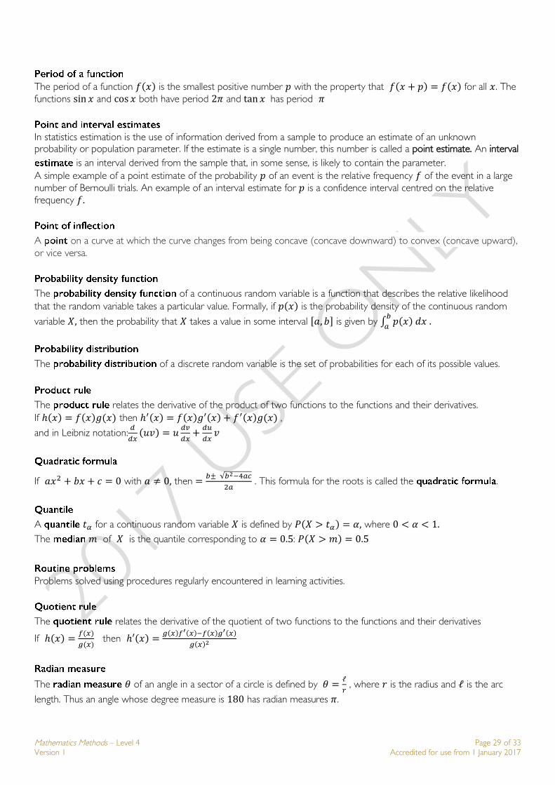
The period of a function 𝑓(𝑥) is the smallest positive number 𝑝 with the property that 𝑓(𝑥 + 𝑝) = 𝑓(𝑥) for all 𝑥. The

functions sin 𝑥 and cos 𝑥 both have period 2𝜋 and tan 𝑥 has period 𝜋

In statistics estimation is the use of information derived from a sample to produce an estimate of an unknown probability or population parameter. If the estimate is a single number, this number is called a point estimate. An interval

is an interval derived from the sample that, in some sense, is likely to contain the parameter.

A simple example of a point estimate of the probability 𝑝 of an event is the relative frequency 𝑓 of the event in a large

number of Bernoulli trials. An example of an interval estimate for 𝑝 is a confidence interval centred on the relative

frequency 𝑓.

A on a curve at which the curve changes from being concave (concave downward) to convex (concave upward),

or vice versa.

The of a continuous random variable is a function that describes the relative likelihood

that the random variable takes a particular value. Formally, if 𝑝(𝑥) is the probability density of the continuous random

variable 𝑋, then the probability that 𝑋 takes a value in some interval [𝑎, 𝑏] is given by ∫ 𝑝(𝑥) 𝑑𝑥 .𝑏

𝑎

The of a discrete random variable is the set of probabilities for each of its possible values.

The relates the derivative of the product of two functions to the functions and their derivatives.

If ℎ(𝑥) = 𝑓(𝑥)𝑔(𝑥) then ℎ′(𝑥) = 𝑓(𝑥)𝑔′(𝑥) + 𝑓′(𝑥)𝑔(𝑥) ,

and in Leibniz notation:𝑑

𝑑𝑥(𝑢𝑣) = 𝑢

𝑑𝑣

𝑑𝑥+

𝑑𝑢

𝑑𝑥𝑣

If 𝑎𝑥2 + 𝑏𝑥 + 𝑐 = 0 with 𝑎 ≠ 0, then =𝑏± √𝑏2−4𝑎𝑐

2𝑎 . This formula for the roots is called the .

A 𝑡𝛼 for a continuous random variable 𝑋 is defined by 𝑃(𝑋 > 𝑡𝛼) = 𝛼, where 0 < 𝛼 < 1.

The 𝑚 of 𝑋 is the quantile corresponding to 𝛼 = 0.5: 𝑃(𝑋 > 𝑚) = 0.5

Problems solved using procedures regularly encountered in learning activities.

The relates the derivative of the quotient of two functions to the functions and their derivatives

If ℎ(𝑥) =𝑓(𝑥)

𝑔(𝑥) then ℎ′(𝑥) =

𝑔(𝑥)𝑓′(𝑥)−𝑓(𝑥)𝑔′(𝑥)

𝑔(𝑥)2

The 𝜃 of an angle in a sector of a circle is defined by 𝜃 =ℓ

𝑟 , where 𝑟 is the radius and ℓ is the arc

length. Thus an angle whose degree measure is 180 has radian measures 𝜋.


A is a numerical quantity, the value of which depends on the outcome of a chance experiment. For

example, the proportion of heads observed in 100 tosses of a coin.

A is one which can only take a countable number of value, usually whole numbers.

A is one whose set of possible values are all of the real numbers in some interval.

If an event 𝐸 occurs 𝑟 times in 𝑛 trials of a chance experiment is, the frequency of 𝐸 is 𝑟

𝑛 .

Problems solved using procedures regularly encountered in learning activities.

A of the graph of a function is a straight line passing through two points on the graph. The line segment between

the two points is called a .

According to the second derivative test, if 𝑓′(𝑥) = 0, then 𝑓(𝑥) is a local maximum of 𝑓 if 𝑓′′(𝑥) < 0 and 𝑓(𝑥) is a

local minimum if 𝑓′′(𝑥) > 0

In the unit circle definition of cosine and sine, cos 𝜃 and sin 𝜃 are the 𝑥 and 𝑦 coordinates of the point on the unit circle

corresponding to the angle 𝜃 measured as a rotation from the ray OX. If is measured in the counter-clockwise direction then it is said to be positive; otherwise it is said to be negative.

The of a random variable is the square root of its variance.

The (or simply the ) to a curve at a given point 𝑃 can be described intuitively as the straight line

that "just touches" the curve at that point. At the point where the tangent touches the curve, the curve has “the same direction” as the tangent line.”. In this sense it is the best straight-line approximation to the curve at the point.

The relates differentiation and definite integrals. It has two forms: 𝑑

𝑑𝑥(∫ 𝑓(𝑡)𝑑𝑡

𝑥

𝑎) =

𝑓(𝑥) and ∫ 𝑓′(𝑥)𝑑𝑥 = 𝑓(𝑏) − 𝑓(𝑎)𝑏

𝑎

The linearity property of anti-differentiation is summarized by the equations:

∫ 𝑘𝑓(𝑥)𝑑𝑥 = 𝑘∫ 𝑓(𝑥)𝑑𝑥 for any constant 𝑘 and ∫ (𝑓1(𝑥) + 𝑓2(𝑥))𝑑𝑥 = ∫ 𝑓1(𝑥)𝑑𝑥 + ∫ 𝑓2(𝑥)𝑑𝑥 for any two

functions 𝑓1(𝑥) and 𝑓2(𝑥). Similar equations describe the linearity property of definite integrals:

∫ 𝑘𝑓(𝑥)𝑑𝑥 = 𝑘 ∫ 𝑓(𝑥)𝑑𝑥𝑏

𝑎

𝑏

𝑎

for any constant 𝑘 and ∫ (𝑓1(𝑥) + 𝑓2(𝑥))𝑑𝑥𝑏

𝑎= ∫ 𝑓1(𝑥)𝑑𝑥

𝑏

𝑎+ ∫ 𝑓2(𝑥)𝑑𝑥

𝑏

𝑎 for any two

functions 𝑓1(𝑥) and 𝑓2(𝑥).


A 𝑋 is one whose probability density function 𝑝(𝑥) has constant value on the

range of possible values of 𝑋. If the range of possible values is the interval [𝑎, 𝑏] then 𝑝(𝑥) =1

𝑏−𝑎 if 𝑎 ≤ 𝑥 ≤ 𝑏

A relation between two real variables 𝑥 and 𝑦 is a function and 𝑦 = 𝑓(𝑥) for some function 𝑓, if and only if each

vertical line, i.e. each line parallel to the 𝑦 −axis, intersects the graph of the relation in at most one point. This test to

determine whether a relation is, in fact, a function is known as the .


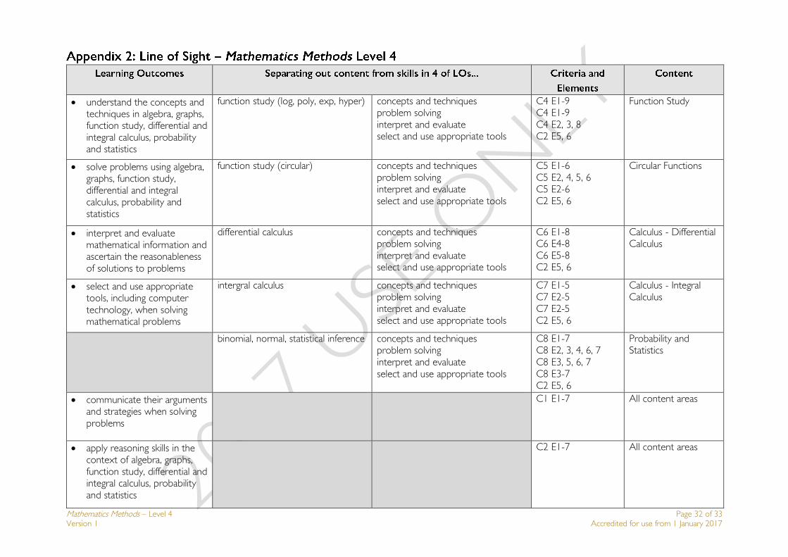
understand the concepts and techniques in algebra, graphs, function study, differential and integral calculus, probability and statistics

function study (log, poly, exp, hyper) concepts and techniques problem solving interpret and evaluate select and use appropriate tools

C4 E1-9 C4 E1-9 C4 E2, 3, 8 C2 E5, 6

Function Study

solve problems using algebra, graphs, function study, differential and integral calculus, probability and statistics

function study (circular) concepts and techniques problem solving interpret and evaluate select and use appropriate tools

C5 E1-6 C5 E2, 4, 5, 6 C5 E2-6 C2 E5, 6

Circular Functions

interpret and evaluate mathematical information and ascertain the reasonableness of solutions to problems

differential calculus concepts and techniques problem solving interpret and evaluate select and use appropriate tools

C6 E1-8 C6 E4-8 C6 E5-8 C2 E5, 6

Calculus - Differential Calculus

select and use appropriate tools, including computer technology, when solving mathematical problems

intergral calculus concepts and techniques problem solving interpret and evaluate select and use appropriate tools

C7 E1-5 C7 E2-5 C7 E2-5 C2 E5, 6

Calculus - Integral Calculus

binomial, normal, statistical inference concepts and techniques problem solving interpret and evaluate select and use appropriate tools

C8 E1-7 C8 E2, 3, 4, 6, 7 C8 E3, 5, 6, 7 C8 E3-7 C2 E5, 6

Probability and Statistics

communicate their arguments and strategies when solving problems

C1 E1-7 All content areas

apply reasoning skills in the context of algebra, graphs, function study, differential and integral calculus, probability and statistics



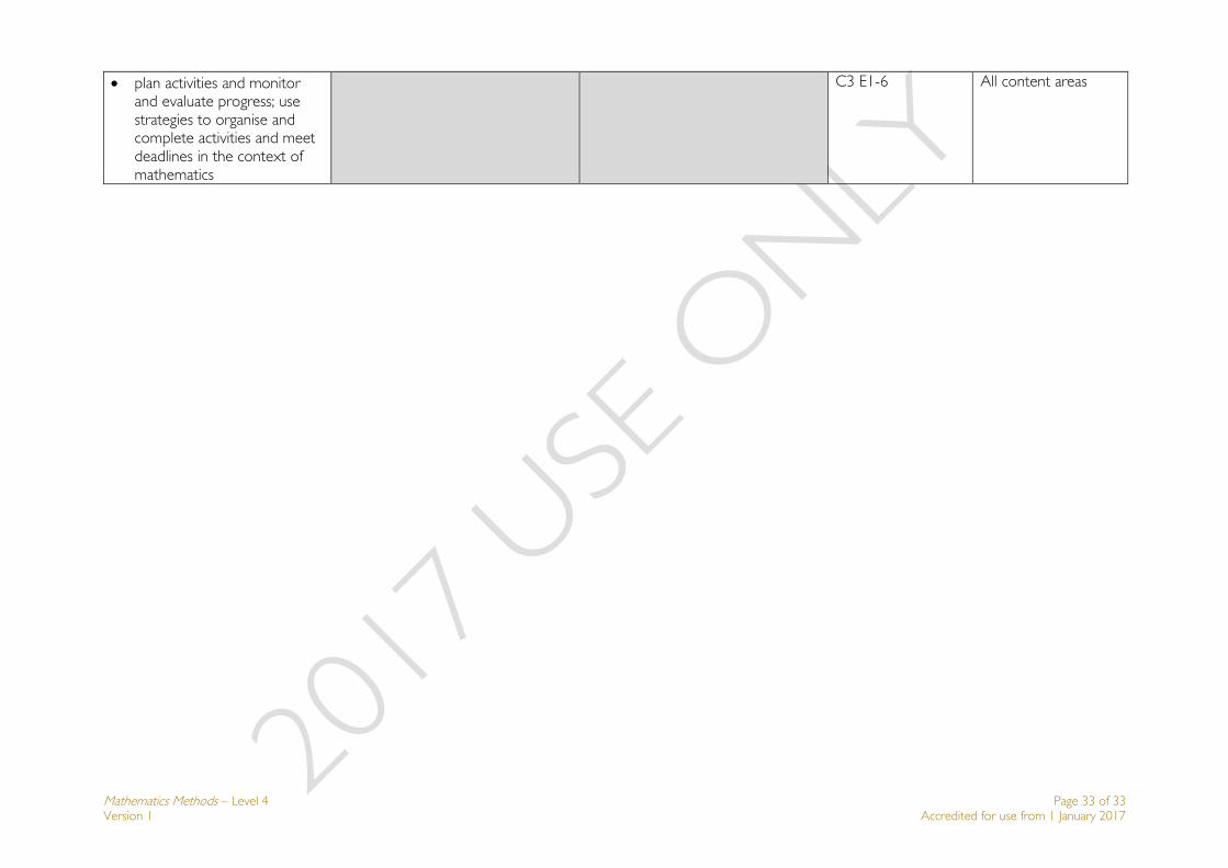
plan activities and monitor and evaluate progress; use strategies to organise and complete activities and meet deadlines in the context of mathematics


mathematics methods - tqa.tas.gov.au · pdf filemathematics methods ... plan activities and...

Documents