Mathematical problems of nonlinear dynamics: A

tutorial

Leonid Shilnikov

Abstract

We review the theory of nonlinear systems, especially that of strange

attractors, and give its perspectives. Of a special attention are the recent

results concerning hyperbolic attractors and features of high-dimensional

systems in the Newhouse regions. We present an example of a “wild”

strange attractor of the topological dimension three.

1

Content

1. Introduction

2. Basic notions of the theory of dynamical systems

3. The Andronov-Pontryagin theorem. Morse-Smale systems

4. Poincare homoclinic structures

5. Structurally stable systems

6. The bifurcation theory. Appearance of hyperbolic attractors

7. Structurally unstable systems. Wild hyperbolic sets. Newhouse regions

8. Lorenz attractor

9. Quasiattractors. Non-transverse homoclinic curves

10. Example of wild strange attractor

2

1 Introduction

The early 60th is the beginning of the intensive development of the theory

of high-dimensional dynamical systems. Within a short period of time Smale

[66, 67] had established the basics of the theory of structurally unstable systems

with the complex behaviour of trajectories, the theory which we now know as

the hyperbolic theory. In essence, a new mathematical discipline with its own

terminology, notions etc, has been created, which at the same time interacts

actively with other mathematical disciplines. Here we must emphasize the role

of the qualitative theory of differential equation (QTODEs). In fact, this theory

provides a foundation for investigating many problems of natural sciences and

engineering which have a nonlinear dynamics origin. On the other hand the

qualitative theory of differential equations itself takes new ideas from nonlinear

dynamics. The usefulness and the necessity of such a synthesis were clear for

such scientists with the broad vision on science as Poincare and Andronov. All

this makes the QTODEs especially attractive and practical. Its achievements

have led to one of the brightest scientific discoveries of the XX century — dy-

namical chaos. Since the moment of the discovery of dynamical chaos along

with such customary dynamical regimes as stationary states, self-oscillations

and modulations, chaotic oscillations entered the science. If the mathemati-

cal images of the formers are equilibrium states, periodic orbits and tori with

quasiperiodic trajectories, then the adequate image of dynamical chaos is a

strange attractor, i.e., an attractive limiting set with the unstable behaviour of

its trajectories. Those attractors that persist this property under small smooth

perturbations will interest us in this review. Namely, such attractors have been

predicted by the hyperbolic theory of high-dimensional dynamical systems.

However, the role and the significance of strange attractors were not accepted

by researchers of certain scientific directions, in particular of turbulence, for a

sufficiently long time. There were a few reasons for that. The hyperbolic theory

had examples of strange attractors but their structure were so topologically

3

complex that did not allow one to imagine rather simple scenarios of their

origination which is very important for nonlinear dynamics, which deals with

models described by differential equations. On the other hand, those “strange

attractors” observed in concrete models were not hyperbolic attractors in the

strict meaning of these words. Most of them, possessing all the properties of a

“qenuine” strange attractor, had stable periodic orbits. This gave a chance to

argue that the observable chaotic behaviour is intermittent. Here, we have to

bear in mind that when speaking about dynamical systems we are interested

not in the character of a solution over some bounded period of time but in

the information on its limiting behaviour when time increases to infinity. Note

also strange attractors that have hyperbolic subsets co-existing with stable long

periodic orbits of very narrow and tortious attraction basin, the so-called quasi-

1attractors [10].

The breakthrough came in the mid 70-ths with the appearance of a “simple”

low-dimensional modelx = −σ(x− y),y = rx− y − xz,z = −bz + xy

in which Lorenz had discovered numerically in 1962 a chaotic behaviour in

the trajectories. A detailed analysis carried out by mathematicians revealed

the existence of a strange attractor, not hyperbolic but non-structurally stable.

Nevertheless, the main feature — the instability of the behaviour of trajectories

under small smooth perturbations of the system — of this attractor persists.

Such attractors, which contain a single equilibrium state of the saddle type,

will be henceforth be called Lorenz(ian) attractors. The second remarkable fact

related to these attractors is that the Lorenz attractor may be generated on the

route of a finite number of rather simple observable bifurcations from systems

with trivial dynamics.

Since that time the phenomenon of dynamical chaos was “almost legislated”.

In this breakthrough, the fact that the Lorenz model came from hydrodynamics

played not the least but a primary role.

The topological dimension of the Lorenz attractor, regardless of the dimen-

1stochastic

4

sion of the associated concrete system, is always two and its fractal dimension

is less than three. At the same time, researchers who deal with extended sys-

tems often observe chaotic regimes of presumably much higher dimensions. It

is customary then to say that hyperchaos occurs. But which attractors describe

hyperchaos? Are they strange attractors or quasiattractors? In principal, the

hyperbolic theory predicts the possibility of the existence of strange attractor

of any finite dimensions. The tragedy is that nobody has observed known hy-

perbolic attractors in nonlinear dynamics since the moment of their invention.

There has been some progress recently: the author and Turaev [79] have proved

that a number of hyperbolic attractors (structurally like the Smale-Williams

solenoids and the Anosov tori) may be obtained through one global bifurcation

of the disappearance of a stable periodic orbit or of an invariant torus with a

quasi-periodic trajectory on it. They have also discovered a principally new

type of strange attractor — the so-called wild strange attractors. Their distinc-

tion from the known attractors is that they contain an equilibrium state of the

saddle-focus type as well as saddle periodic trajectories of various types, namely,

dimensions of invariant manifolds of the co-existing trajectories may be equal

both two and three. Moreover, the region of the existence of such an attractor is

a region of everywhere dense structural instability due to homoclinic tangencies.

Thus, the above phenomenon poses principally new problems for ergodic theory.

Due to the co-existence of the trajectories of various types the wild attractors,

as well as Lorenz-like attractors, are the pseudo-hyperbolic attractors. Since

the notion of pseidohyperbolicity, which plays a dominating role in the theory

of structurally unstable strange attractors, will be used below. So let us stop

here and discuss it in detail.

Consider a smooth n-dimensional dynamical system

x = X(x),

in a bounded region D which satisfies the following conditions:

1. On its boundary ∂D the vector flow goes inward D. This implies that for

any point x ∈ ∂D either an entire trajectory or a semitrajectory is defined

that passes through the point x.

5

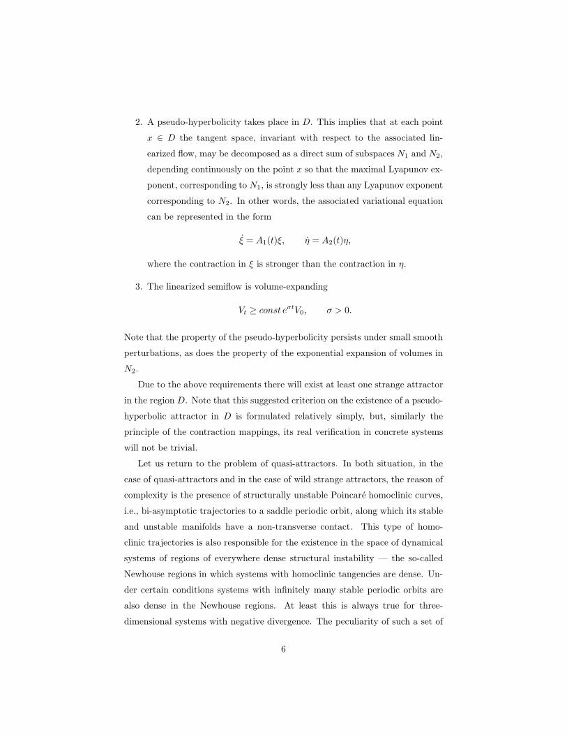
2. A pseudo-hyperbolicity takes place in D. This implies that at each point

x ∈ D the tangent space, invariant with respect to the associated lin-

earized flow, may be decomposed as a direct sum of subspaces N1 and N2,

depending continuously on the point x so that the maximal Lyapunov ex-

ponent, corresponding to N1, is strongly less than any Lyapunov exponent

corresponding to N2. In other words, the associated variational equation

can be represented in the form

ξ = A1(t)ξ, η = A2(t)η,

where the contraction in ξ is stronger than the contraction in η.

3. The linearized semiflow is volume-expanding

Vt ≥ const eσtV0, σ > 0.

Note that the property of the pseudo-hyperbolicity persists under small smooth

perturbations, as does the property of the exponential expansion of volumes in

N2.

Due to the above requirements there will exist at least one strange attractor

in the region D. Note that this suggested criterion on the existence of a pseudo-

hyperbolic attractor in D is formulated relatively simply, but, similarly the

principle of the contraction mappings, its real verification in concrete systems

will not be trivial.

Let us return to the problem of quasi-attractors. In both situation, in the

case of quasi-attractors and in the case of wild strange attractors, the reason of

complexity is the presence of structurally unstable Poincare homoclinic curves,

i.e., bi-asymptotic trajectories to a saddle periodic orbit, along which its stable

and unstable manifolds have a non-transverse contact. This type of homo-

clinic trajectories is also responsible for the existence in the space of dynamical

systems of regions of everywhere dense structural instability — the so-called

Newhouse regions in which systems with homoclinic tangencies are dense. Un-

der certain conditions systems with infinitely many stable periodic orbits are

also dense in the Newhouse regions. At least this is always true for three-

dimensional systems with negative divergence. The peculiarity of such a set of

6

stable periodic orbits is that it cannot be separated in a quasiattractor from

the co-existing hyperbolic subset to which these periodic orbits accumulate. In

three-dimensional systems with sigh-alternating divergences, for example in the

Chua circuit [22, 45] , the situation is even more sophisticated [77]. Namely, to-

tally unstable (repelling) periodic orbits may coexist with the hyperbolic subset

and the set of stable periodic orbits with very long periods. A similar hier-

archy will occur in high-dimensional quasi-attractors in which stable periodic

orbits, invariant tori as well as stable strange attractors of various topological

dimensions may be imbedded in an extremely non-trivial way. Apart from very

well developed stability windows where these stable objects reveal themselves,

they are practically invisible in numerical experiments because they have very

long transients and weak attraction basins since they are closely mixed with the

hyperbolic structure.

The above observations show that a careful and correct interpretation of

many applied studies on dynamical chaos is essential. In particular, this includes

the activity related to the calculation of Lyapunov exponents on a finite interval

of time. The justification of this calculation is based on Oseledec’s theorem [52]

on the majority of the Lyapunov-right trajectories in the sense of a suitable

measure. Apparently, one needs to account for the effect of small probabilistic

noise which can blur the subtle (delicate) structure of quasi-attractors.

Andronov had proposed a recipe on the analysis of concrete models. The

basic idea is the following:

1. Partitioning the parameter space into regions of structural stability and

identifying the bifurcation set;

2. Dividing the bifurcation set into connected components corresponding to

qualitatively similar, in the sense of topological equivalence, phase por-

traits.

Nowadays, Andronov’s program has not lost its practicality except for some

important corrections. Namely, in situations when a system admits the existence

of non-transverse homoclinic curves typical for quasi-attractors, wild attractors,

etc., since structurally unstable systems may fill out entire regions in the space

7

of dynamical systems. As established by Gonchenko, Shilnikov and Turaev

[33, 34] the following C r-smooth (r ≥ 3) systems are everywhere dense in the

Newhouse regions

1. systems having infinitely many periodic orbits of any order of degeneracy;

2. systems with homoclinic tangencies of any order.

Consequently, we can make the following important conclusion; namely the

goal of a complete investigation of systems with complex dynamics of above

types is unrealistic. It appears that one should abandon the ideology of a com-

plete description and turn to the study of some special but distinctive properties

of the system. The properties which are worth studying must essentially depend

on the nature of the problem.

2 Basic notions of the theory of dynamical sys-

tems

Three components are employed in the definition of a dynamical system. 1)

A metric space E called the phase space. 2) A time variable t which may be

either continuous, i.e., t ∈ R1, or discrete, i.e., t ∈ Z. 3) An evolution law,

i.e., a mapping of any given point x in E and any t to a uniquely defined state

ϕ(t, x) ∈ E. It is also assumed that the following conditions hold:

1. ϕ(0, x) = x.

2. ϕ(t1, ϕ(t2, x)) = ϕ(t1 + t2, x),

3. ϕ(t, x) ∈ C0 with respect to (t, x).

(2.1)

In the case where t is continuous the above conditions define a continuous

dynamical system, or flow. In other words, a flow is a one-parameter group

of homeomorphisms 2 of the phase space E. Fixing x and varying t from −∞2i.e., one-to-one, continuous mappings with a continuous inverse. This follows directly

from the group property (2.1).

8

to +∞ we obtain an orientable curve 3 which, as before, we will call a phase

trajectory. The following sub-division of phase trajectories is natural: equi-

librium states, periodic trajectories and unclosed trajectories. We will call a

positive semi-trajectory

x;ϕ(t, x), t ≥ 0

and

x;ϕ(t, x), t ≤ 0

a negative

semi-trajectory. Observe that in the case of an unclosed trajectory any point of

the trajectory partitions the trajectory into two parts: a positive semi-trajectory

and a negative semi-trajectory.

In the case where the mapping ϕ(t, x) is a diffeomorphism 4 the flow is a

smooth dynamical system In this case the phase space E must be endowed with

some additional structures. The phase space E is usually chosen to be either

Rn, or Rn−k×Tk, where Tk = S1×S1× · · ·×S1 may be a k-dimensional torus,

a smooth surface, or a manifold. This allows us to set up a correspondence

between smooth flow and associated vector fields by defining a velocity field

V (x) =dϕ(t, x)

dt

∣∣∣t=0

. (2.2)

The simplest but the most principal case of a smooth dynamical system is the

flow determined by the vector field

x = X(x), x ∈ Rn,

where X ∈ Cr, r ≥ 1.

Discrete dynamical systems are, more briefly, called cascades. A cascade

possesses the following remarkable feature. Let us select a homeomorphism

ϕ(1, x) and denote it by ϕ(x). It is obvious that ϕ(t, x) = ϕt(x), where

ϕt = ϕ (ϕ(. . . ϕ(x)))︸ ︷︷ ︸

t times

.

Hence, in order to define a cascade it is sufficient only to point out the homeo-

morphism ϕ : E 7→ E.

In the case of a discrete dynamical system a sequence

xk

+∞

−∞where xk+1 =

ϕ(xk), is called the trajectory of a point x0. Trajectories may be of three types:

3which defines the direction of motion4a one-to-one, differentiable mapping with differentiable inverse.

9

1. A point x0. The point is a fixed point of the homeomorphism ϕ(x), i.e.,

it is mapped by ϕ(x) onto itself.

2. A cycle (x0, . . . , xk−1), where xi = ϕk(xi), i = (0, . . . , k − 1) and where,

moreover, xi 6= xj for i 6= j. The number k is called the period of the

cycle, and the point xi is called a periodic point of period k. Observe that

a fixed point is a periodic point of period 1.

3. A bi-infinite (i.e., infinite in both directions) sequence

xk

+∞

−∞, where

xi 6= xj for i 6= j. In this case, as in the case of flows, we will say that

such a trajectory is unclosed.

When ϕ(x) is a diffeomorphism, the cascade is a smooth dynamical sys-

tem. Examples of cascades of this type are non-autonomous periodic systems.

Consider the system

x = X(x, t),

where X(x, t) is defined and continuous with respect to all variables in Rn×R1,

is smooth with respect to x and periodic of period τ with respect to t, and has

solutions which may be continued over the interval 0 ≤ t ≤ τ . Given a solution

x = ϕ(t, x0), where ϕ(0, x0) = x0 we may define the mapping

x1 = ϕ(τ, x) (2.3)

of the hyper-plane t = 0 into the hyper-plane t = τ . It follows from the period-

icity of X(x, t) that (x, t1) and (x, t2) must be identified if (t2 − t1) is divisibleby τ . Thus, (2.3) may be regarded as a diffeomorphism ϕ : Rn 7→ Rn. 5

Among cascades of special interest are the so-called topological Markov chains

(TMC). Let us define a TMC. Let G be an orientable multigraph such that

each vertex is the beginning of a certain edge, and at the same time, the end

of the same edge or another edge. Let us enumerate the edges of G by symbols

5Observe that in this case system (2.3) may be written as an autonomous system

x = X(x, θ), θ = 1,

where θ is taken in modulo τ .

10

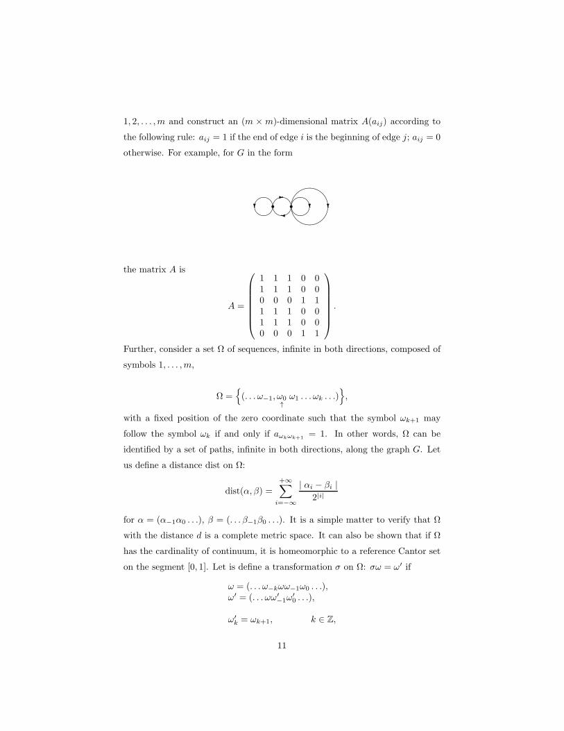
1, 2, . . . ,m and construct an (m × m)-dimensional matrix A(aij) according to

the following rule: aij = 1 if the end of edge i is the beginning of edge j; aij = 0

otherwise. For example, for G in the form

r r

the matrix A is

A =

1 1 1 0 01 1 1 0 00 0 0 1 11 1 1 0 01 1 1 0 00 0 0 1 1

.

Further, consider a set Ω of sequences, infinite in both directions, composed of

symbols 1, . . . ,m,

Ω =

(. . . ω−1, ω0↑ω1 . . . ωk . . .)

,

with a fixed position of the zero coordinate such that the symbol ωk+1 may

follow the symbol ωk if and only if aωkωk+1= 1. In other words, Ω can be

identified by a set of paths, infinite in both directions, along the graph G. Let

us define a distance dist on Ω:

dist(α, β) =

+∞∑

i=−∞

| αi − βi |2|i|

for α = (α−1α0 . . .), β = (. . . β−1β0 . . .). It is a simple matter to verify that Ω

with the distance d is a complete metric space. It can also be shown that if Ω

has the cardinality of continuum, it is homeomorphic to a reference Cantor set

on the segment [0, 1]. Let is define a transformation σ on Ω: σω = ω′ if

ω = (. . . ω−kωω−1ω0 . . .),ω′ = (. . . ωω′

−1ω′0 . . .),

ω′k = ωk+1, k ∈ Z,

11

i.e., in the sequence ω the position of the zero coordinate is translated (shifted)

by one symbol to the right: (. . . ω−1ω0ω1 . . .).

The transformation σ is called a shift. It can be easily verified that σ is

single-valued and continuous together with the inverse mapping σ−1. It is the

cascade (σk,Ω) which is called TMC, and this will be denoted hereafter as

(G,Ω, σ). If there exists a path from any vertex of the graph G to any other

one, σ | Ω is transitive, and if , moreover, h = lnλ1, σ has a countable set of

periodic points and they are everywhere dense in Ω. Here λ1 is the maximal

eigenvalues of the matrix A, and h is the topological entropy of the mapping σ.

Introduce also the notion of a suspension over TMC. In the direct product

Ω × I, where I is the segment [0, 1], we identify the points (ω, 1) and (σω, 1)

for all ω ∈ Ω. The topological space thus obtained is the phase space of such a

system and is denoted by Σ. 6 Let us define a flow T t on Σ by the following

relation:

T t(ω, s) =

(ω, t+ s),(σω, t+ s− 1),

if − s < t ≤ 1− sif 1− s < t ≤ 1

and for the rest, t ∈ R1, the flow is defined by the condition that T t forms a

group (e.g., for −1 < t ≤ −s, T t(ω, s) = (σ−1ω, 1 + t+ s), etc). It can be seen

that the mapping T t preserves the set of points (ω, 0) = Ω invariant and acts

on it exactly as σ does. In other words, σ is the Poincare map of the transversal

Ω of the phase space Σ for the flow T t.

Before proceeding further, we need to introduce some notions.

A set A is said to be invariant with respect to a homeomorphism ϕ if

A = ϕ(t, A) for any t. Here, ϕ(t, A) denotes the set⋃

x∈A

ϕ(t, x). It follows from

this definition that if x ∈ A, then the trajectory ϕ(t, x) lies in A.

We call a point x0 wandering if there exists an open neighborhood U(x0) of

x0 and a positive integer T such that

U(x0) ∩ ϕ(t, U(x0)) = ∅ for t > T. (2.4)

Applying the transformation ϕ(−t, x) to (2.4) we obtain

6Σ may be provided with a metric.

12

ϕ(−t, U(x0)) ∩ U(x0) = ∅ for t < T.

Hence, the definition of a wandering point is symmetric with respect to the

positive and negative values of t.

Let us denote by W the set of non-wandering points. The set W is open

and invariant. Openness follows from the fact that together with x0 any point

in U(x0) is wandering. The invariance of W follows from the fact that if x0 is

a wandering point, then the point ϕ(t0, x0) is also a wandering point for any

t0. To show this let us choose ϕ(t0, U(x0)) to be the neighborhood of the point

ϕ(t0, x0). Then

ϕ(t0, U(x0)) ∩ ϕ(t, ϕ(t0, U(x0)) = ∅ for t > T.

Hence, the set of non-wandering pointsM = D\W is closed and invariant. The

set of non-wandering points may be empty. To illustrate the latter consider a

dynamical system defined by the autonomous system

x = X(x, θ), θ = 1,

with phase space Rn+1, x = (x1, . . . , xn).

It is clear that equilibrium states, as well as all points on periodic trajec-

tories, are non-wandering. All points on bi-asymptotic trajectories which tend

to equilibrium states and periodic orbits as t → ±∞ are also non-wandering.

Bi-asymptotic trajectories are unclosed and are called homoclinic trajectories.

The points on Poisson-stable trajectories are also non-wandering points

Definition. A point x0 is said to be positive Poisson-stable if given any

neighborhood U(x0) and any T > 0 there exists t > T such that

ϕ(t, x0) ⊂ U(x0). (2.5)

If there exists t such that t < −T and (2.5) holds, then the point x0 is called a

negative Poisson-stable point. If point x0 is both positive and negative Poisson

stable it is said to be Poisson-stable, (see Fig. 2.1).

13

Observe that if the point x0 is positive (negative) Poisson-stable, then any

point of the trajectory ϕ(t, x0) is also positive (negative) Poisson stable. Thus,

we may introduce the notion of a P+-trajectory for a positive Poisson-stable

trajectory, a P−-trajectory for a negative Poisson-stable trajectory and merely

a P -trajectory for a Poisson-stable trajectory. It follows directly from (2.5) that

P+, P− and P -trajectories consist of non-wandering points.

It is obvious that equilibrium states and periodic orbits are closed P -trajectories.

Denote by Σ the closure of P+ (P−, P )-trajectory.

Theorem 2.1 (Birkhoff If a P+ (P−, P )-trajectory is unclosed, then Σ contains

a continuum of unclosed P -trajectories.

Let us choose a positive sequence of

Tn

where Tn → +∞ as n → +∞.

It follows from the definition of a P+-trajectory that there exists a sequence

tn

→ +∞ as n→ +∞ such that ϕ(tn, x0) ⊂ U(x0). An analogous statement

holds in the case of a P−-trajectory. This implies that a P -trajectory succes-

sively intersects any ǫ-neighborhoodUǫ(x0) of the point x0 infinitely many times.

7 Let

tn(ǫ)+∞

−∞be such that tn(ǫ) < tn+1(ǫ) and let ϕ(tn(ǫ), x0) ⊂ Uǫ(x0).

We introduce the notion of the Poincare return times

τn(ǫ) = tn+1(ǫ)− tn(ǫ).

Two essentially different cases are possible for an unclosed P -trajectory:

1. the sequence

τn(ǫ)

is bounded, i.e., there exists a number L(ǫ) such

that τn(ǫ) < L(ǫ) for any n. Observe that L(ǫ)→ +∞ as ǫ→ 0.

2. The sequence

τn(ǫ)

is unbounded.

In the first case the P -trajectory is called recurrent. For such a trajectory

all trajectories in its Σ closure are also recurrent, and the closure itself is a

minimal set 8. The principal property of a recurrent trajectory is that it returns

to an ǫ-neighborhood of the point x0 within a time not greater than L(ǫ).

7In the case of flows the P -trajectory intersects Uǫ(x0) for values of t in an infinite set ofintervals In(ǫ) where tn(ǫ) is one of the times in In(ǫ).

8a set is called minimal if it is non-empty, invariant, closed and contains no proper subsetspossessing these three properties.

14

However, in contrast to periodic orbits, whose return times are known, the

return time for a recurrent trajectory is not constrained. Among recurrent

trajectories we may also select a more narrow class of motions, the so-called

almost-periodic trajectories. There is no uncertainty in the Poincare return

times of such a trajectory since it comes back to its neighbourhood over its

almost-period τ(ǫ). Almost-periodic trajectories may be sub-divided into the

two sub-classes: quasiperiodic and limit-quasiperiodic trajectories. In the case

of smooth flows the minimal set of the quasi-periodic trajectories is a torus,

whereas the minimal set of the limit-periodic trajectories is a rather non-trivial

set, called a solenoid. The local structure of a solenoid may be defined by a

direct product Rm ×K where K is the Cantor discontinuum.

In the second case, the closure Σ of the P -trajectory is called a quasi-minimal

set. There always exist in Σ other invariant closed subsets which may be equi-

librium states, periodic trajectories or invariant tori, etc. Since the P -trajectory

may approach such subsets arbitrarily closely, the Poincare return times can be

arbitrarily large. Suppose that for a trajectory L given by the equation x = ϕ(t)

the closure of the semi-trajectory L+ (L−) for t ≥ t0 (t ≤ t0) is a compact set.

Definition The point x0 is called an ω-limiting point of the trajectory L if

there exists a sequence

tk

where tk → +∞ as k →∞ such that

liml→∞

ϕ(tk) = x∗.

A similar definition for an α-limiting point tk → −∞ as k →∞. We denote

the set of all ω-limiting points of the trajectory L by ΩL and that of the α-

limit points we denote by AL. Observe that an equilibrium state has a unique

limit point, namely, itself. In the case where the trajectory L is periodic all

of its points are α and ω-limit points, i.e., L = ΩL = AL. In the case where

L is an unclosed Poisson-stable trajectory the sets ΩL and AL coincide with

its closure L. This L is either a minimal set if L is a recurrent trajectory,

or a quasi-minimal set if the return Poincare times of L are unbounded. All

equilibrium states, periodic trajectories and Poisson-stable trajectories are said

to be self-limit trajectories.

15

The structure of the sets ΩL (AL) has been almost completely studied for

two-dimensional dynamical systems on the plane where the trajectory remains

in some bounded domain of the plane as t→ +∞ (t→ −∞).

Both sets ΩL and AL are well know to be invariant and closed. In the case

when the system under consideration is a flow, ΩL (AL) is then a connected set.

Poincare and Bendixson established that the set ΩL may be of one of the

following topological types:

I. Equilibrium states.

II. Periodic trajectories.

III. Contours composed of equilibrium states and connecting trajectories tend-

ing to these equilibrium states as t→ ±∞.

Fig. 2.2 represents examples of limit sets of the third type where we label the

equilibrium states by O. Using the general classification above we may enumer-

ate all types of positive semi-trajectories of planar systems:

1. equilibrium states;

2. periodic trajectories;

3. semi-trajectories tending to an equilibrium state;

4. semi-trajectories tending to a periodic trajectory;

5. semi-trajectories tending to a limit set of type III.

Observe that an analogous situation occurs in the case of negative semi-trajectories.

In the general case, besides the above types of limiting sets the closure of tra-

jectories of flows on two-dimensional compact surfaces may also be a minimal

set as well as a quasi-minimal set.

Let us discuss the second problem concerning the study of the totality of

trajectories. In fact, determining a dynamical system means topological (or

qualitative) partitioning the structure of the phase space by trajectories of dif-

ferent topological types, or in other words, finding its phase portrait. This poses

the question of when two phase portraits are similar. In terms of the qualitative

16

theory of dynamical systems we can answer this question by introducing the

notion of to the so-called topological equivalence.

Definition Two systems are said to be topologically equivalent if there exists

a homeomorphism of the phase spaces which maps trajectories (semi-trajectories,

intervals of a trajectory) of one system into trajectories (semi-trajectories, in-

tervals of a trajectory) of the second.

This implies that equilibrium states are mapped into equilibrium states,

periodic trajectories and unclosed trajectories of one system are mapped into

equilibrium states, periodic trajectories and unclosed trajectories of another

system. The topological equivalence of two systems in some sub-regions of the

phase space is defined in the similar manner. The latter is used while study-

ing local problems, for example, while studying the equivalence of structures of

trajectories in a neighborhood of an equilibrium state, or near periodic or ho-

moclinic trajectories. This definition of two topologically equivalent dynamical

systems is an indirect definition of the notion of the topological or qualitative

structure of the partition of the phase space into trajectories. We may say that

such a structure preserves all properties of the partition which remain invariant

with respect to all possible homeomorphisms applied to the phase space.

Let G be a bounded sub-region of the phase space and let H = hi be a

set of homeomorphisms of G mapping trajectory into trajectory of the same

topological types. Then we can introduce a metric distance as follows

dist(h1, h2) = supx∈G‖h1x− h2x‖.

Definition We call a trajectory L ∈ G particular if there exists ǫ > 0 such

that for all h satisfying dist(h, I) < ǫ, where I is the identity homeomorphism,

the following condition holds

hL = L.

It is clear that all equilibrium states and periodic orbits are particular tra-

jectories. Unclosed trajectories may be particular also. For example, particular

17

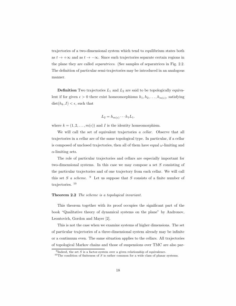
trajectories of a two-dimensional system which tend to equilibrium states both

as t→ +∞ and as t→ −∞. Since such trajectories separate certain regions in

the plane they are called separatrices. (See samples of separatrices in Fig. 2.2.

The definition of particular semi-trajectories may be introduced in an analogous

manner.

Definition Two trajectories L1 and L2 are said to be topologically equiva-

lent if for given ǫ > 0 there exist homeomorphisms h1, h2, . . . , hm(ǫ), satisfying

dist(hk, I) < ǫ, such that

L2 = hm(ǫ) · · ·h1L1.

where k = (1, 2, . . . ,m(ǫ)) and I is the identity homeomorphism.

We will call the set of equivalent trajectories a cellar. Observe that all

trajectories in a cellar are of the same topological type. In particular, if a cellar

is composed of unclosed trajectories, then all of them have equal ω-limiting and

α-limiting sets.

The role of particular trajectories and cellars are especially important for

two-dimensional systems. In this case we may compose a set S consisting of

the particular trajectories and of one trajectory from each cellar. We will call

this set S a scheme. 9 Let us suppose that S consists of a finite number of

trajectories. 10

Theorem 2.2 The scheme is a topological invariant.

This theorem together with its proof occupies the significant part of the

book “Qualitative theory of dynamical systems on the plane” by Andronov,

Leontovich, Gordon and Mayer [2].

This is not the case when we examine systems of higher dimensions. The set

of particular trajectories of a three-dimensional system already may be infinite

or a continuum even. The same situation applies to the cellars. All trajectories

of topological Markov chains and those of suspensions over TMC are also par-

9Indeed, the set S is a factor-system over a given relationship of equivalence.10The condition of finiteness of S is rather common for a wide class of planar systems.

18

ticular.

Definition An attractor is a closed invariant set A which possesses a neigh-

borhood (an absorbing area) U(A) such that the trajectory ϕ(t, x) of any point

x in U(A) satisfies the condition

dist((ϕ(t, x), A)→ 0 as t→ +∞, (2.6)

where

dist(x,A) = infx0∈A

‖x, x0‖.

The simplest examples of attractors are stable equilibrium states, stable peri-

odic trajectories and stable invariant tori containing quasi-periodic trajectories,

which satisfy (2.6).

This definition of an attractor does not preclude the possibility that it may

contain other attractors. It is reasonable to restrict the notion of an attractor

by requiring a quasi-minimality condition. The essence of this requirement is

that A is to be a transitive set. A set M is said to be transitive if it contains an

everywhere dense trajectory L, e.g., L = M . The most interesting attractors

are the so-called strange attractors which are invariant, closed sets composed

of only unstable trajectories which are, in fact, the particular trajectories. The

theme of strange attractors and of mechanisms of their appearance is of special

attention in this paper.

3 Andronov-Pontryagin theorem. Morse-Smale

systems

We will assume that all dynamical systems under consideration to be in the

form

x = X(x),

where x ∈ C1 and are defined in some closed, bounded region G ⊂ Rn. For such

19

vector fields we can introduce a norm as follows

‖X‖C1 = supx∈G

(

‖X(x)‖+∥∥∥∥

∂X(x)

∂x

∥∥∥∥

)

.

Having introduced this norm the set of dynamical system becomes a Banach

space of dynamical systems.

Definition. The system X(x) is called rough in G if an ǫ > 0 there exists

δ > 0 such that if ‖X − X‖ < δ, then X and a neighboring system X are

topologically equivalent. Moreover, the conjugating homeomorphism h is close

to the identity homeomorphism I, i.e., dist(h, I) < ǫ.

This definition was first introduced by Andronov and Pontryagin under the

additional requirement that the boundary ∂G of the region G is a surface with-

out a contact, e.g., the vector field is transverse to ∂G and, moreover is directed

inward G.

The problem of defining the region G does not exist if we consider vector

fields on compact, smooth manifolds. In this situation the notion of the rough-

ness may be introduced in a similar manner with the only difference that the

associated vector field is a Banach manifold.

Another notion close to the notion of the roughness is that of structural

stability

Definition The system X(x) is called structurally stable in G if there exists

an ǫ > 0 such that if ‖X −X‖ < ǫ, then X and X are topologically equivalent.

It follows immediately from this definition that structurally stable systems

form an open set in the Banach space of dynamical systems, whereas in the

case of rough systems this is not so obvious. Nevertheless, the notion of a

rough system is more “physical” in the sense that it reflects the fact that small

perturbations of the original vector field cause small changes of the associated

phase portrait. However, it follows from recent on structurally stable systems

that there exist always δ-homeomorphisms.

For two-dimensional system of the form

x = P (x, y),y = Q(x, y)

(3.1)

Andronov and Pontryagin proved the following theorem

20

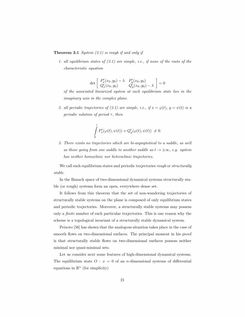
Theorem 3.1 System (3.1) is rough if and only if

1. all equilibrium states of (3.1) are simple, i.e., if none of the roots of the

characteristic equation

det

[P ′x(x0, y0)− λ P ′

y(x0, y0)Q′x(x0, y0) Q′

y(x0, y0)− λ

]

= 0

of the associated linearized system at each equilibrium state lies in the

imaginary axis in the complex plane.

2. all periodic trajectories of (3.1) are simple, i.e., if x = ϕ(t), y = ψ(t) is a

periodic solution of period τ , then

τ∫

0

P ′x(ϕ(t), ψ(t)) +Q′

y(ϕ(t), ψ(t)) 6= 0.

3. There exists no trajectories which are bi-asymptotical to a saddle, as well

as those going from one saddle to another saddle as t→ ±∞, e.g. system

has neither homoclinic nor heteroclinic trajectories.

We call such equilibrium states and periodic trajectories rough or structurally

stable.

In the Banach space of two-dimensional dynamical systems structurally sta-

ble (or rough) systems form an open, everywhere dense set.

It follows from this theorem that the set of non-wandering trajectories of

structurally stable systems on the plane is composed of only equilibrium states

and periodic trajectories. Moreover, a structurally stable systems may possess

only a finite number of such particular trajectories. This is one reason why the

scheme is a topological invariant of a structurally stable dynamical system.

Peixoto [56] has shown that the analogous situation takes place in the case of

smooth flows on two-dimensional surfaces. The principal moment in his proof

is that structurally stable flows on two-dimensional surfaces possess neither

minimal nor quasi-minimal sets.

Let us consider next some features of high-dimensional dynamical systems.

The equilibrium state O : x = 0 of an n-dimensional systems of differential

equations in Rn (for simplicity)

21

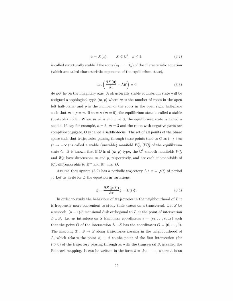
x = X(x), X ∈ Ck, k ≤ 1, (3.2)

is called structurally stable if the roots (λ1, . . . , λn) of the characteristic equation

(which are called characteristic exponents of the equilibrium state),

det

(∂X(0)

∂x− λE

)

= 0 (3.3)

do not lie on the imaginary axis. A structurally stable equilibrium state will be

assigned a topological type (m, p) where m is the number of roots in the open

left half-plane, and p is the number of the roots in the open right half-plane

such that m+ p = n. If m = n (m = 0), the equilibrium state is called a stable

(unstable) node. When m 6= n and p 6= 0, the equilibrium state is called a

saddle. If, say for example, n = 3, m = 3 and the roots with negative parts are

complex-conjugate, O is called a saddle-focus. The set of all points of the phase

space such that trajectories passing through these points tend to O as t→ +∞(t → −∞) is called a stable (unstable) manifold W s

O (WuO of the equilibrium

state O. It is known that if O is of (m, p)-type, the Ck-smooth manifolds W sO

and WuO have dimensions m and p, respectively, and are each submanifolds of

Rn, diffeomorphic to Rm and Rp near O.

Assume that system (3.2) has a periodic trajectory L : x = ϕ(t) of period

τ . Let us write for L the equation in variations:

ξ =∂X(ϕ(t))

∂xξ = B(t)ξ. (3.4)

In order to study the behaviour of trajectories in the neighbourhood of L it

is frequently more convenient to study their traces on a transversal. Let S be

a smooth, (n− 1)-dimensional disk orthogonal to L at the point of intersection

L ∪ S. Let us introduce on S Euclidean coordinates s = (s1, . . . , sn−1) such

that the point O of the intersection L ∪ S has the coordinates O = (0, . . . , 0).

The mapping T : S 7→ S along trajectories passing in the neighbourhood of

L, which relates the point s0 ∈ S to the point of the first intersection (for

t > 0) of the trajectory passing through s0 with the transversal S, is called the

Poincare mapping. It can be written in the form u = Au + · · · , where A is an

22

(n − 1) × (n − 1)-dimensional matrix whose eigenvalues are multipliers of the

periodic trajectory L.

A set of all points of the phase space, such that trajectories passing through

these points tend to L as t→ +∞ (t→ −∞) is called a stable (unstable) mani-

fold W sL (Wu

L ) of the periodic orbit L. It is clear that L belongs simultaneously

both toW sL andWu

L . The manifoldsW sL andWu

L are each smooth submanifolds

of Rn in the neighborhood of their points, and have the dimensions m and p,

respectively. For n = 2 and m = p = 2, W sL (Wu

L) is homeomorphic to a Mobius

band, if the multiplier which is less (greater) than 1, in modulus, is negative,

and to a cylinder if it is positive. In the latter case divides W sL (Wu

L ) into two

unconnected pieces, see Fig. 3.1.

Let us now define the transverse intersection of stable and unstable mani-

folds. Let W sL1 and WuL2 be stable and unstable manifolds of periodic tra-

jectories or equilibrium states, and W sL1∩Wu

L26= ∅. W s

L1and Wu

L1are said to

intersect each other transversally if

dimTxWsL1

+ dimTxWuL2− n = dim(TxW

sL1∪ TxWu

L2), (3.5)

where TxWsL1

(TxWuL2) denotes a tangent to W s

L1(Wu

L2) at the point x. The

property of intersection transversality does not change under small perturba-

tions of a system and is, in this case, a structurally stable one. Let us note

that a saddle periodic trajectory L belongs to the transverse intersection of its

stable and unstable manifolds. All other trajectories belonging to W sL ∩ Wu

L

are homoclinic curves (or trajectories). Those of the curves along which W s

and Wu intersect transversally are called structurally stable homoclinic curves.

Select one more type of trajectories which connect saddle equilibrium states or

(and) saddle periodic trajectories such that

dim TxWsL1

+ dimTxWuL2

= n, (3.6)

where L1 6= L2. We will call such trajectories heteroclinic. Observe that all

mentioned trajectories are particular.

Structurally stable diffeomorphisms are introduced in an analogous man-

ner as structurally stable vector fields. Usually, it is added that the following

23

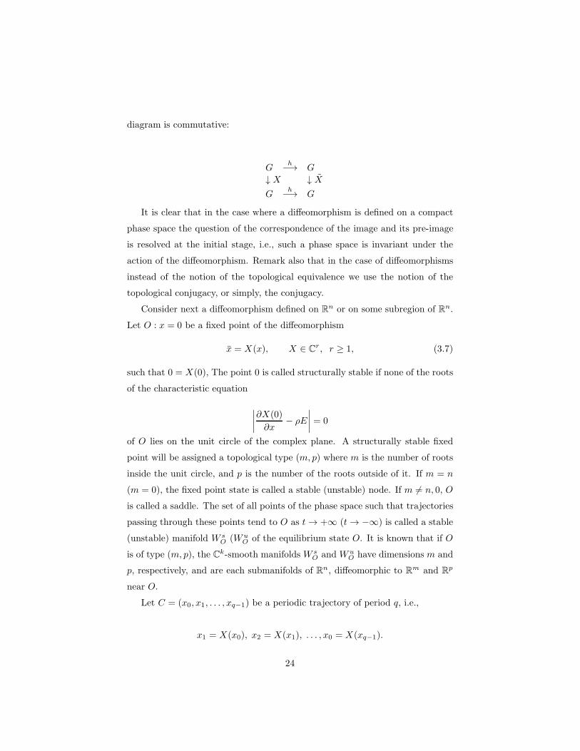
diagram is commutative:

Gh−→ G

↓ X ↓ XG

h−→ G

It is clear that in the case where a diffeomorphism is defined on a compact

phase space the question of the correspondence of the image and its pre-image

is resolved at the initial stage, i.e., such a phase space is invariant under the

action of the diffeomorphism. Remark also that in the case of diffeomorphisms

instead of the notion of the topological equivalence we use the notion of the

topological conjugacy, or simply, the conjugacy.

Consider next a diffeomorphism defined on Rn or on some subregion of Rn.

Let O : x = 0 be a fixed point of the diffeomorphism

x = X(x), X ∈ Cr, r ≥ 1, (3.7)

such that 0 = X(0), The point 0 is called structurally stable if none of the roots

of the characteristic equation

∣∣∣∣

∂X(0)

∂x− ρE

∣∣∣∣= 0

of O lies on the unit circle of the complex plane. A structurally stable fixed

point will be assigned a topological type (m, p) where m is the number of roots

inside the unit circle, and p is the number of the roots outside of it. If m = n

(m = 0), the fixed point state is called a stable (unstable) node. If m 6= n, 0, O

is called a saddle. The set of all points of the phase space such that trajectories

passing through these points tend to O as t→ +∞ (t→ −∞) is called a stable

(unstable) manifold W sO (Wu

O of the equilibrium state O. It is known that if O

is of type (m, p), the Ck-smooth manifolds W sO and Wu

O have dimensions m and

p, respectively, and are each submanifolds of Rn, diffeomorphic to Rm and Rp

near O.

Let C = (x0, x1, . . . , xq−1) be a periodic trajectory of period q, i.e.,

x1 = X(x0), x2 = X(x1), . . . , x0 = X(xq−1).

24

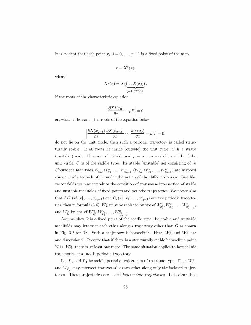
It is evident that each point xi, i = 0, . . . , q − 1 is a fixed point of the map

x = Xq(x),

where

Xq(x) = X((. . .X(x)))︸ ︷︷ ︸

q−1 times

.

If the roots of the characteristic equation

∣∣∣∣

∂Xq(x0)

∂x− ρE

∣∣∣∣= 0,

or, what is the same, the roots of the equation below

∣∣∣∣

∂X(xq−1)

∂x

∂X(xq−2)

∂x· · · ∂X(x0)

∂x− ρE

∣∣∣∣= 0,

do not lie on the unit circle, then such a periodic trajectory is called struc-

turally stable. If all roots lie inside (outside) the unit cycle, C is a stable

(unstable) node. If m roots lie inside and p = n − m roots lie outside of the

unit circle, C is of the saddle type. Its stable (unstable) set consisting of m

Ck-smooth manifolds W sx0,W s

x1, . . . ,W s

xq−1(Wu

x0,Wu

x1, . . . ,Wu

xq−1) are mapped

consecutively to each other under the action of the diffeomorphism. Just like

vector fields we may introduce the condition of transverse intersection of stable

and unstable manifolds of fixed points and periodic trajectories. We notice also

that if C1(x10, x

11, . . . , x

1q1−1) and C2(x

20, x

21, . . . , x

2q2−1) are two periodic trajecto-

ries, then in formula (3.6),W sL must be replaced by one ofW s

x10

,W sx11

, . . . ,W sx1q1−1

,

and WuL by one of Wu

x20

,Wux21

, . . . ,Wux2q1−1

.

Assume that O is a fixed point of the saddle type. Its stable and unstable

manifolds may intersect each other along a trajectory other than O as shown

in Fig. 3.2 for R2. Such a trajectory is homoclinic. Here, W sO and Wu

O are

one-dimensional. Observe that if there is a structurally stable homoclinic point

W sO ∩Wu

O, there is at least one more. The same situation applies to homoclinic

trajectories of a saddle periodic trajectory.

Let L1 and L2 be saddle periodic trajectories of the same type. Then W sL1

and WuL2

may intersect transversally each other along only the isolated trajec-

tories. These trajectories are called heteroclinic trajectories. It is clear that

25

both homoclinic and heteroclinic trajectories along which stable and unstable

manifolds intersect transversally, are structurally stable.

Let us now consider the class of C1-smooth dynamical systems satisfying the

following conditions:

1. The non-wandering set consists of a finite number of structurally stable

equilibrium states and periodic orbits.

2. The stable and unstable manifolds of equilibrium states, and periodic tra-

jectories, intersect transversally.

Such systems are called Morse-Smale systems. They are structurally stable

as it was established by Palis and Smale. In a certain sense the Morse-Smale

systems are a high-dimensional generalization of rough systems of Andronov

and Pontryagin. In contrast to the Andronov-Pontryagin systems which have

only a finite number of particular trajectories, the set of such trajectories, in

particular homoclinic amd heteroclinic trajectories, in the Morse-Smale system

may be countable. Afraimovich and Shilnikov [15] have shown that the existence

heteroclinic trajectories being unclosed, particular trajectories of the Morse-

Smale systems may, in particular, leads to a complex structure of the wandering

set. Loci of heteroclinic trajectories may be described in the language of the

suspensions over topological Markov chains.

We see that the Morse-Smale systems comprise a simpler class amongst all

high-dimensional dynamical systems. However, it appears that we can only

point out one complete topological invariant for the Morse-Smale systems. The

only known result deals with three-dimensional systems with a finite number of

particular trajectories [82]. 11

Let is discuss next the Morse-Smale diffeomorphisms.

A diffeomorphism is called a Morse-Smale diffeomorphism if it satisfies the

following conditions:

1. Its wandering set consists of a finite number of structurally stable periodic

trajectories. 12

11The problem of finding a complete topological invariant for systems which nowadays arecalled Morse-Smale systems was posed by Andronov.

12A fixed point is a periodic trajectory of period 1.

26

2. Stable and unstable manifolds of periodic trajectories intersect transver-

sally.

There exits also the problem of finding a complete topological invariant. This

problem has been studied only for diffeomorphisms on closed, two-dimensional

surfaces provided that the diffeomorphism is either gradient-like, or has an ori-

entable heteroclinic set, or has a finite set of heteroclinic trajectories [12, 14].

A common feature of both Morse-Smale flows and cascades is the absence

of cycles.

Definition Let L1 · · ·Lq be either an equilibrium state or a periodic tra-

jectory, and let Γ1, . . . ,Γq be trajectories satisfying the following conditions:

Ω(Γk) = Lk+1 and A(Γk) = Lk, (k = 1, q − 1), Ω(Γq) = L1 and A(Γq) = Lq.

Here we denote by Ω and A the ω-limiting set and the α-limiting set, respec-

tively. The collection (L1,Γ1, . . . , Lq,Γq) is then called a cycle.

Furthermore, the Morse-Smale system cannot have cycles which contain

equilibrium states and periodic trajectories both of different topological types

since this violates the condition of transversality for some homoclinic or hete-

roclinic trajectories. Otherwise, if we suppose Morse-Smale system have such

a cycle, it is only possible when all Li’s are periodic trajectories, and of the

same type. We can show then that each Li has a structurally stable homoclinic

trajectory and, as a result, a countable number of saddle periodic trajectories in

its neighborhood which contradicts the definition of the Morse-Smale systems.

4 Poincare homoclinic structures

While studying the bounded problem of three bodies in the Cartesian mechan-

ics Poincare discovered homoclinic structures [57]. He established that if the

stable and unstable manifolds of a saddle periodic trajectory intersect along

one homoclinic curve, then there are also infinitely many of such curves. The

theme of studying of Poincare homoclinic curves was continued by Birkhoff who

proved the existence of a countable set of periodic trajectories in a neighbor-

hood of a homoclinic curve of a volume-preserving diffeomorphism. Andronov

was the next who posed the problem of constructing structurally stable three-

27

dimensional flows and two-dimensional diffeomorphisms possessing homoclinic

structures, or, in other words, having a countable set of periodic trajectories.

The essence of the problem is the following. Consider a periodically forced

non-autonomous system

x = P (x, y) + µp(t),y = Q(x, y) + µq(t),

(4.1)

where p(t) and q(t) are periodic functions of period τ . Assume that when µ = 0

(4.1) has a homoclinic loop Γ(0) to a saddle point at the origin O(0, 0). When

µ 6= 0 system (4.1) may be represented as an autonomous system of the form

x = P (x, y) + µp(θ),y = Q(x, y) + µq(θ),

θ = 1(4.2)

in the phase space R2 × S1. In fact, for all µ sufficiently small we may reduce

the study of (4.2) to the consideration of the Poincare map on the cross-section

θ = 0. For small µ the diffeomorphism

x = F (x, y),y = G(x, y) + µq(θ), θ mod 2π,

(4.3)

has a fixed point O(µ) of the saddle type. Moreover, the stableW sO and unstable

WuO manifolds of the point O(µ) may transversally intersect each other along the

homoclinic curve Γ(µ) for all ‖µ‖ < µ0.13 One can show that within the interval

‖µ‖ < µ0 there exits a countable set of values of µ at which the intersection

W sO and Wu

O is no longer transverse. Therefore, apriori we cannot exclude the

existence of regions of everywhere dense structural instability. This problem

was resolved by Smale who presented a simple example of a two dimensional

diffeomorphism which is structurally stable and at the same time has a non-

wandering invariant set Ω homeomorphic to a Bernoulli subshift on two symbols.

The Bernoulli subshift is a particular case of topological Markov chains whose

graph has the following form

13such a situation occurs, for instance, when the Melnikov function used for estimating thesplitting of separatrices, has simple zeros citeME63.

28

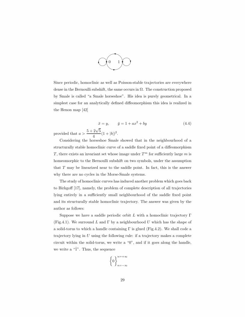
r1r 0

Since periodic, homoclinic as well as Poisson-stable trajectories are everywhere

dense in the Bernoulli subshift, the same occurs in Ω. The construction proposed

by Smale is called “a Smale horseshoe”. His idea is purely geometrical. In a

simplest case for an analytically defined diffeomorphism this idea is realized in

the Henon map [42]

x = y, y = 1 + ax2 + by (4.4)

provided that a >5 + 2

√5

4(1 + |b|)2.

Considering the horseshoe Smale showed that in the neighbourhood of a

structurally stable homoclinic curve of a saddle fixed point of a diffeomorphism

T , there exists an invariant set whose image under Tm for sufficiently large m is

homeomorphic to the Bernoulli subshift on two symbols, under the assumption

that T may be linearized near to the saddle point. In fact, this is the answer

why there are no cycles in the Morse-Smale systems.

The study of homoclinic curves has induced another problem which goes back

to Birkgoff [17], namely, the problem of complete description of all trajectories

lying entirely in a sufficiently small neighbourhood of the saddle fixed point

and its structurally stable homoclinic trajectory. The answer was given by the

author as follows:

Suppose we have a saddle periodic orbit L with a homoclinic trajectory Γ

(Fig.4.1). We surround L and Γ by a neighbourhood U which has the shape of

a solid-torus to which a handle containing Γ is glued (Fig.4.2). We shall code a

trajectory lying in U using the following rule: if a trajectory makes a complete

circuit within the solid-torus, we write a “0”, and if it goes along the handle,

we write a “1”. Thus, the sequence

0

n=+∞

n=−∞

29

corresponds to the periodic orbit L. The sequence

. . . 0, 0, 1, 0, 0, . . .

corresponds to the homoclinic orbit Γ. The sequence

jn

n=+∞

n=−∞

, jn = 0, 1

corresponds to an arbitrary trajectory within U . Moreover, each 1 is followed

by zeros whose number is not fewer than k, where k depends on the size of the

neighbourhood: the narrower neighbourhood U we choose the bigger k will be.

There is another more suitable algorithm of coding. Introduce a symbol

1 =

[

1,

k︷ ︸︸ ︷

0, . . . , 0

]

.

Then we obtain a new truncated sequence

jn

n=+∞

n=−∞

, jn = 0, 1

for such a trajectory, where jn can be followed by either 1 or 0. In other words,

the set of trajectories lying in U is in correspondence with the Bernoulli scheme

on two symbols. 14 Moreover, in this case the converse statement is valid also.

Let us illustrate this statement with an example of a diffeomorphism T

x = λx+ P (x, y),y = γy +Q(x, y),

(4.5)

where 0 < λ < 1, γ > 1, and P (x, y) and Q(x, y) vanish at the origin O(0, 0)

along with their first derivatives. In this case, O is a fixed point of the saddle

type. Assume that its manifolds W s and Wu intersect transversally along a

homoclinic curve Γ. Let us choose a pair of homoclinic points M+ and M− in

a small neighbourhood of O such that M+ ∈ W sloc and M− ∈ Wu

loc. Surround

the point M+ by a small rectangle Π+ and the point M− by a small rectangle

Π− as shown in Fig.4.3. The condition of smallness of both rectangles is that

they do not intersect with their images under the map T . Then, inside Π+ and

Π− we may define a countable set of “strips” σ0k and σ1

k, where k ≤ k, k is

14To be more precise, this set is homeomorphic to a suspension over the Bernoulli scheme.

30

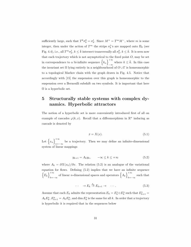
sufficiently large, such that T kσ0k = σ1

k. Since M+ = TmM−, where m is some

integer, then under the action of Tm the strips σ1k’s are mapped onto Π0 (see

Fig. 4.4), i.e., all Tmσ1k, k ≤ k intersect transversally all σ0

k, k ≤ k. It is seen now

that each trajectory which is not asymptotical to the fixed point O, may be set

in correspondence to a bi-infinite sequence

kα

+∞

−∞where k ≤ k. In this case

the invariant set Ω lying entirely in a neighbourhood of O ∪Γ is homeomorphic

to a topological Markov chain with the graph drawn in Fig. 4.5. Notice that

accordingly with [15] the suspension over this graph is homeomorphic to the

suspension over a Bernoulli subshift on two symbols. It is important that here

Ω is a hyperbolic set.

5 Structurally stable systems with complex dy-

namics. Hyperbolic attractors

The notion of a hyperbolic set is more conveniently introduced first of all on

example of cascades ϕ(k, x). Recall that a diffeomorphism in Rn inducing as

cascade is denoted by

x = X(x). (5.1)

Let

xn

+∞

n=−∞be a trajectory. Then we may define an infinite-dimensional

system of linear mappings

yk+1 = Akyk, −∞ ≤ k ≤ +∞ (5.2)

where Ak = ∂X(xk)/∂x. The relation (5.2) is an analogue of the variational

equation for flows. Defining (5.2) implies that we have an infinite sequence

Ek

+∞

k=−∞of linear n-dimensional spaces and operators

Ak

+∞

k=−∞such that

· · · → EkAk→ Ek+1 → · · · . (5.3)

Assume that each Ek admits the representation Ek = Esk⊗Euk such that Esk+1 =

AkEsk, E

uk+1 = AkE

uk , and dimEsk is the same for all k. In order that a trajectory

is hyperbolic it is required that in the sequences below

31

· · · → EskAk→ Esk+1 → · · ·

· · · ← EukA−1

k← Euk+1 ← · · · .(5.4)

there exists an uniform contraction of the exponential type.

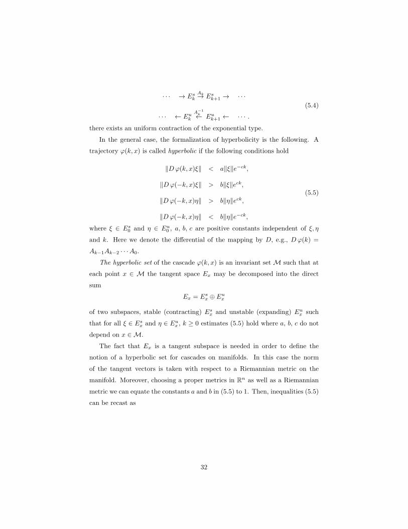
In the general case, the formalization of hyperbolicity is the following. A

trajectory ϕ(k, x) is called hyperbolic if the following conditions hold

‖Dϕ(k, x)ξ‖ < a‖ξ‖e−ck,

‖Dϕ(−k, x)ξ‖ > b‖ξ‖eck,

‖Dϕ(−k, x)η‖ > b‖η‖eck,

‖Dϕ(−k, x)η‖ < b‖η‖e−ck,

(5.5)

where ξ ∈ Es0 and η ∈ Eu0 , a, b, c are positive constants independent of ξ, η

and k. Here we denote the differential of the mapping by D, e.g., Dϕ(k) =

Ak−1Ak−2 · · ·A0.

The hyperbolic set of the cascade ϕ(k, x) is an invariant setM such that at

each point x ∈ M the tangent space Ex may be decomposed into the direct

sum

Ex = Esx ⊕ Eux

of two subspaces, stable (contracting) Esx and unstable (expanding) Eux such

that for all ξ ∈ Esx and η ∈ Eux , k ≥ 0 estimates (5.5) hold where a, b, c do not

depend on x ∈M.

The fact that Ex is a tangent subspace is needed in order to define the

notion of a hyperbolic set for cascades on manifolds. In this case the norm

of the tangent vectors is taken with respect to a Riemannian metric on the

manifold. Moreover, choosing a proper metrics in Rn as well as a Riemannian

metric we can equate the constants a and b in (5.5) to 1. Then, inequalities (5.5)

can be recast as

32

‖Dϕ(1, x)ξ‖ ≤ λ‖ξ‖,

‖Dϕ(−1, x)ξ‖ > 1λ‖ξ‖,

‖Dϕ(1, x)η‖ ≥ 1λ‖η‖,

‖Dϕ(−1, x)η‖ < λ‖η‖,

(5.6)

where 0 < λ < 1.

Consider next the case of the flow ϕt determined by the vector field V (x)

on a manifold. The hyperbolic set of such a flow is a compact, invariant setMsuch that

1. if a point of M is an equilibrium state, then the equilibrium state is

hyperbolic, i.e., its eigenvalues do not lie on the imaginary axis in the

complex plane;

2. the setM is closed and at its each point x the tangent space Tx is decom-

posed into the direct sum

Esx ⊕ Eux ⊕ E0

of its linear subspaces, the third of which is generated by the vector of

the phase velocity, and the first two properties are analogous to the case

discrete time case, i.e., Esx and Eux satisfy condition (5.5).

Examples of hyperbolic set are equilibrium states, periodic and heteroclinic

trajectories (including their closures) of the Morse-Smale systems, as well as a

set consisting of the points lying entirely in a neighbourhood of a structurally

stable homoclinic curve.

It is natural that in the general case a hyperbolic set is foliated into non-

intersecting, closed, invariant sets

Mj =

x ∈ M, dimEsx = j

.

Of special interest here are the systems satisfying the condition of hyper-

bolicity in the entire phase space. Such flows and cascades are called Anosov

33

systems. Anosov proved that hyperbolic systems are rough or structurally sta-

ble. The peculiarity of the Anosov systems is that all of their trajectories are

particular. This is a reason of why in the case of the Anosov cascades the home-

omorphism of conjugacy of two close diffeomorphisms is unique. Examples of

the Anosov systems are geodesic flows on compact, smooth manifolds of a neg-

ative curvature [11]. It is well-know such that a flow is conservative and its set

of non-wandering trajectories coincides with the phase space. An example of

the Anosov diffeomorphism is a mapping of an n-dimensional torus

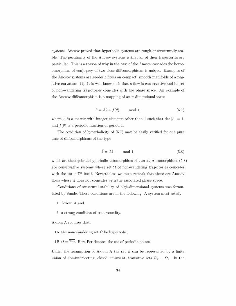
θ = Aθ + f(θ), mod 1, (5.7)

where A is a matrix with integer elements other than 1 such that det |A| = 1,

and f(θ) is a periodic function of period 1.

The condition of hyperbolicity of (5.7) may be easily verified for one pure

case of diffeomorphisms of the type

θ = Aθ, mod 1, (5.8)

which are the algebraic hyperbolic automorphism of a torus. Automorphisms (5.8)

are conservative systems whose set Ω of non-wandering trajectories coincides

with the torus Tn itself. Nevertheless we must remark that there are Anosov

flows whose Ω does not coincides with the associated phase space.

Conditions of structural stability of high-dimensional systems was formu-

lated by Smale. These conditions are in the following: A system must satisfy

1. Axiom A and

2. a strong condition of transversality.

Axiom A requires that:

1A the non-wandering set Ω be hyperbolic;

1B Ω = Per. Here Per denotes the set of periodic points.

Under the assumption of Axiom A the set Ω can be represented by a finite

union of non-intersecting, closed, invariant, transitive sets Ω1, . . .Ωp. In the

34

case of cascades, any such Ωi can be represented by a finite number of sets

having these properties which are mapped to each other under the action of the

diffeomorphism. The sets Ω1, . . .Ωp are called basis sets.

A condition of strong transversality is the following: the location of the

manifolds W sL1

and WuL2

of any two trajectories L1 and L2 is in the general

position, i.e., they either do not intersect each other, or intersect each other

transversally. We remark that by virtue of the Hadamard-Perron theorem each

hyperbolic trajectory has its stable and unstable manifolds whose smoothness

is equal to the smoothness of the system.

Theorem 5.1 (Robinson) If a dynamical system satisfies Axiom A and the

condition of the strong transversality, then the system is structurally stable.

As for necessary conditions we have the following theorem

Theorem 5.2 (Mane [46]) A structurally stable cascade satisfies Axiom A and

the condition of strong transversality.

In the case of flows there are no explicit statements of the same kind. Never-

theless, it follows, more or less, from a series of resent results that the conditions

formulated by Smale are necessary for flows also.

The basis sets of Smale systems (satisfying the enumerated conditions) may

be of the following three types: attractors, repellers and saddles. Repellers are

the basis sets which becomes attractors in backward time. Saddle basis sets

are such that may both attract and repel outside trajectories. A most studied

saddle basis sets are one-dimensional in the case of flows and null-dimensional

in the case of cascades. The former ones are homeomorphic to the suspension

over topological Markov chains; the latter ones are homeomorphic to simple

topological Markov chains [Bowen [18]]. As for other basis sets the situation is

more difficult. Currently we do not have any proper classification for them. It

is known only that some may be obtained from Markov systems under suitable

gluing and change of time [Bowen [19]].

Attractors of Smale systems are called hyperbolic. The trajectories passing

sufficiently close to an attractor of a Smale system, satisfies the condition

35

dist(ϕ(t, x), A) < ke−λt, t ≥ 0

where k and λ are some positive constants. As we have said earlier these at-

tractors are transitive. Periodic, homo- and heteroclinic trajectories as well

as Poisson-stable ones are everywhere dense in them. In particular, we can

tell one more of their peculiarity: the unstable manifolds of all points of such

an attractor lie within it, i.e., W sx ∈ A where x ∈ A. Hyperbolic attractors

may be smooth or non-smooth manifolds, have a fractal structure, not locally

homeomorphic to a direct product of a disk and a Cantor set.

Below we will discuss a few hyperbolic attractors which might be curious

for nonlinear dynamics. The first example of such a hyperbolic attractor is the

Anosov torus Tn with a hyperbolic structure on it. The next example of hy-

perbolic attractor was designed by Smale on a two-dimensional torus by means

of a “surgery” operation over the automorphism of this torus with a hyperbolic

structure. This is the so-called DA-(derived from Anosov) diffeomorphism. An

original two-dimensional diffeomorphism is taken in the form

θ1 = a11θ1 + a12θ2, mod 1,θ2 = a21θ1 + a22θ2, mod 1

(5.9)

This diffeomorphism possesses two invariant foliations given by equations

θ1 = λ1θ1 + c1, mod 1,θ2 = λ2θ2 + c2, mod 1,

(5.10)

where λ1 and λ2 are the roots of the characteristic equation

∣∣∣∣

a11 − λ a12a21 a22 − λ

∣∣∣∣, (5.11)

and c1 and c2 are constant, 0 ≤ c1,2 < 1. Both roots, due to assumptions

of hyperbolicity, are always irrational. The stable foliation corresponds to the

root |λ1| < 1, the unstable foliation corresponds to the second root |λ2| > 1.

The leaves of the stable (unstable) foliation are the stable (unstable) manifolds

of the points of the torus. The operation over the linear automorphism is as

follow: a small rectangle is chosen in a neighbourhood of the origin O. Within

this rectangle the diffeomorphism is modified so that the stable foliation of the

36

altered diffeomorphism coincides with that of the old diffeomorphism with the

only difference of one leaf passing through the point O. The point O breaks it

into two parts. Moreover, choosing the perturbation such that on this particular

layer two new hyperbolic fixed points appear to the left and to the right of O

whereas the point O becomes totally unstable, i.e., a repeller. The closure of

one of the two new fixed points is an attractor, see Fig. 5.1, Thus, the new dif-

feomorphism possesses an attractor, a repeller and a set consisting of wandering

trajectories. It is interesting to note that the construction of such attractors is

designed as that of minimal sets known from the Poincare-Donjoy theory in the

case of C1-smooth vector fields on a two-dimensional torus [24].

Let us consider a solid torus Π ∈ Rn, i.e., T2 = D2 × S1 where D2 is a

disk and S1 is a circumference. We now expand T2 m-times (m is an integer)

along the cyclic coordinate on S1 and shrink it q-times along the diameter of

D2 where q ≤ 1/m. We then embed this deformated torus Π1 into the original

one so that its intersection with D2 consists of m-smaller disks as shown in

Fig.5.2. Repeat this routine with Π1 and so on. The set Σ =∈∞i=1 Πi so

obtained is called a Witorius-Van Danzig solenoid. Its local structure may be

represented as the direct product of an interval and a Cantor set. Smale also

observed that Witorius-Van Danzig solenoids may have a hyperbolic structures,

i.e., be hyperbolic attractors of diffeomorphisms on solid tori. Moreover, similar

attractors can be realized as a limit of the inverse spectrum of the expanding

cycle map [84]

θ = mθ, mod 1.

The peculiarity of such solenoids is that they are expanding solenoids. Generally

speaking, an expanding solenoid is called a hyperbolic attractor such that its

dimension coincides with the dimension of the unstable manifolds of the points

of the attractor. Expanding solenoids were studied by Williams [85] who showed

that they are generalized (extended) solenoids. The construction of generalized

solenoids is similar to that of minimal sets of limit-quasi-periodic trajectories.

Note that in the theory of sets of limit-quasi-periodic functions the Wictorius-

Van Danzig solenoids are quasi-minimal sets. Hyperbolic solenoids are called

the Smale-Williams solenoids. We return to them in section 7.

37

We remark also on an example of a hyperbolic attractor of a diffeomorphism

on a two-dimensional sphere, and, consequently, on the plane, which was built by

Plykin. In fact, this is a diffeomorphism of a two-dimensional torus projected

onto a two-dimensional sphere. Such a diffeomorphism, in the simplest case,

possesses not three fixed points as in Smale’s example, but four fixed points, all

of them repelling.

As for the question of finding complete topological invariants of structurally

stable systems with non-trivial dynamics, this concerns mainly Anosov diffeo-

morphisms and two-dimensional diffeomorphisms on surfaces. We refer the

reader to the issue [13, 14].

To conclude this section we remark that structurally stable high-dimensional

systems are not dense in the space of all dynamical systems.

6 Everywhere density of structurally unstable

systems. Newhouse regions

As we have noticed above that amongst all two-dimensional flows the struc-

turally stable ones form an open and dense set in the space of dynamical sys-

tems. This is not the case for multi-dimensional flows. Smale was the first who

noted it.

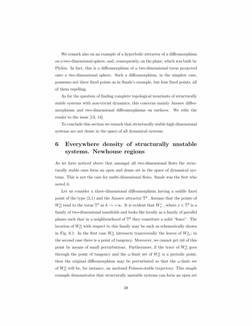
Let us consider a three-dimensional diffeomorphism having a saddle fixed

point of the type (2,1) and the Anosov attractor T2. Assume that the points of

WuO tend to the torus T2 as k → +∞. It is evident that W s

x , where x ∈ T2 is a

family of two-dimensional manifolds and looks like locally as a family of parallel

planes such that in a neighbourhood of T2 they constitute a solid “fence”. The

location of WuO with respect to this family may be such as schematically shown

in Fig. 6.1. In the first case W sO intersects transversally the leaves of W s

T2 ; in

the second case there is a point of tangency. Moreover, we cannot get rid of this

point by means of small perturbations. Furthermore, if the trace of WuO goes

through the point of tangency and the ω-limit set of WuO is a periodic point,

then the original diffeomorphism may be perturbated so that the ω-limit set

of WuO will be, for instance, an unclosed Poisson-stable trajectory. This simple

example demonstrates that structurally unstable systems can form an open set

38

in the space of dynamical systems. But in such a case there is structural in-

stability on the non-wandering set. Then, it is rather reasonable to weaken the

requirement of structural stability up to that of Ω-stability, where Ω denotes

the set of non-wandering points.

Definition. A dynamical system X is called Ω-stable (Ω-rough) if given ǫ

there exists δ > 0 such that for any system X ǫ-close in C1-metrics to X the

set Ω(X) is homeomorphic to Ω(X); moreover the homeomorphism is ǫ-close to

the identity homeomorphism.

In other words, the non-wandering set is preserved under small perturba-

tions; it is only shifted a little bit.

Assume that our flow satisfies Axiom A. Then, as we know, Ω = A1∪· · ·∪Ak.Let us introduce the following relationship Ai > Aj which means that in the

phase space there exists a point x such that the ω-limit set of its trajectory

ϕ(t, x) lies in Aj and the corresponding α-limit set lies in Ai. It may appear

that there is a chain

Ai1 > · · · > Aik > Ai1 ,

i.e., it is not a partially ordered set and, therefore, there are cycles in it. If there

are no cycles, we say that acyclicity takes place.

Theorem 6.1 (Smale) If a dynamical system satisfies Axiom A and the con-

dition of acyclicity, then this system is Ω-stable.

The condition of acyclicity is essential. Although Ai persists under small

perturbations they may cause the so-called Ω-explosion.

Nevertheless, Ω-stable systems are also not dense in the space of dynamical

systems. Example of such systems are strange attractors of the Lorenz type

(which we will discuss below) and “wild” hyperbolic attractors.

Let us consider a diffeomorphism possessing an Ω-stable null-dimensional

hyperbolic set Σ which is homeomorphic to a transitive Markov chain, for ex-

ample, to the non-wandering set of the Smale horseshoe. Since this set is of

39

the saddle type, we may define W sΣ and Wu

Σ . W sΣ (W s

Σ) is a union of stable

(unstable) manifolds of the points of Σ. Since both W sΣ and W s

Σ are “hole”-like

sets, each can be represented by a direct product of an interval and a Cantor

set. Assume that W sΣ and W s

Σ behave as shown in Fig. 6.2. Newhouse noted

that in the case of C2-smooth diffeomorphisms if there are points x1 and x2

in Σ such that W sx1

and Wux2

have a quadratic tangency, then under certain

conditions all C2-close diffeomorphisms preserve this tangency. Such Σ-sets are

called wild hyperbolic sets.

In essence, this problem is reduced to the problem of the existence of regions

of everywhere dense structural instability of systems close to a system with a

structurally unstable homoclinic trajectory. Here, we have a result proved by

Newhouse

Theorem 6.2 (Newhouse) In any neighbourhood of a Cr-smooth (r ≥ 2) two-

dimensional diffeomorphism having a saddle fixed point with a structurally un-

stable homoclinic trajectory there exist regions where systems with structurally

unstable homoclinic trajectories are dence everywhere.

These regions are called Newhouse regions.

Let us denote by B1 the set of diffeomorphisms which possess a saddle point

O whose stable and unstable manifolds have a quadratic tangency along a homo-

clinic curve. Consider a one-parameter familyXµ of two-dimensional Cr-smooth

diffeomorphisms such that Xµ is transverse to B1 at µ = 0.

Theorem 6.3 (Newhouse) Given sufficiently small µ0, the interval (−µ0, µ0)

contains a countable set of Newhouse intervals.

This theorem is especially important for many problems of nonlinear dynam-

ics since it guarantees the existence of the Newhouse regions in finite-parameter

models. The Newhouse results were generalized for the multi-dimensional case

by Gonchenko, Shilnikov and Turaev [33].

The study of systems with a structurally unstable homoclinic trajectory was

started by Gavrilov and Shilnikov in [26]. It was established that the typical

40

systems with quadratic homoclinic tangencies may be classified with respect to

the character of the sets N lying entirely in a small but fixed neighbourhood of

the homoclinic trajectory Γ:

1. N = O ∩ Γ. This situation occurs, for example, in the case of a two-

dimensional diffeomorphism with |λγ| < 1 at 0, see Fig. 6.3a. Under small

perturbations, which lead to the appearance of infinitely many structurally

stable homoclinic trajectories, the structure of a neighbourhood of Γ is

non-trivial. This is the Ω-explosion.

2. N admits a precise description. For flows, N is homeomorphic to a sus-

pension over a Bernoulli shift on 3 symbols in which two trajectories are

glued. An example is shown in Fig. 6.3b.

3. N contains a hyperbolic set but does not admit a precise description.

In the bifurcation set B1 of such systems those systems, which have a

countable set of structurally unstable periodic trajectories of any degree

of degeneracy, as well as systems having a countable set of structurally

unstable homoclinic trajectories of any order of tangency, are everywhere

dense. A possible situation is shown in Fig. 6.3c. Observe that homoclinic

tangencies of the third type are everywhere dense in the Newhouse regions.

The “wild” hyperbolicity accomplishes one more principal case. Consider a

Cr, (r ≥ 4)-smooth system. Assume that the following conditions are fulfilled.

1. At the origin the system has an equilibrium state of the saddle-focus type,

i.e., the root λ1, . . . , λn of the characteristic equation at O are such that

λ1,2 = ρ± iω, ω 6= 0,Reλi < −ρ, i = 3, . . . , n− 1σ = −ρ+ λn > 0.

In this case dimWuO = 1 and dimW s

O = n− 1.

2. Assume that one of two separatrices of the saddle-focus comes back to O

as t→ +∞, see Fig. 6.4.

41

3. As t → +∞ Γ tends to O tangentially to a two-dimensional hyper-plane

corresponding to the eigenvalues λ1 and λ2.

4. A certain value, called a separatrix value, which characterizes the global

behaviour of Γ is non-zero.

The systems with the above properties form a subset of B1 of codimension one

in the space of dynamical systems with C3 metrics.

Shilnikov [71, 73] established that the behaviour of the trajectories in a

neighbourhood of the separatrix Γ is rather complicated. In these works he fo-

cused on the separation of the set of hyperbolic trajectories and its description

via the language of symbolic dynamics. In Ovsyannikov and Shilnikov [53, 54]

it was established that everywhere dense structural instability takes place on

B1. In particular, the following theorem was proven:

Theorem 6.4 In B1 the system with

1. structurally unstable periodic trajectories

and

2. structurally unstable Poincare homoclinic curves

are everywhere dense.

Further, in section 10, we present an example of an n, (n ≥ 4)-dimensional

system possessing a wild attractor including a saddle-focus.

7 Bifurcations of dynamical systems. Blue sky

catastrophe. Appearance of hyperbolic at-

tractors

We will discuss here the border bifurcations which lead us out of the class of

Morse-Smale systems to systems with complex dynamics. Such bifurcations

interest us in the context of scenarios of the appearance of strange attractors,

i.e., the routes to dynamical chaos.

42

The violation of the condition of the structural stability of Morse-Smale

systems may occur in the following three cases:

1. The lost of the condition of hyperbolicity of equilibrium states or periodic

trajectories.

2. The lost of the condition of intersection transversality of stable and unsta-

ble manifolds of equilibrium states and periodic trajectories, both of the

saddle type.

3. The formation of cycles (see the definition is section 3).

Due to the huge volume of existing materials an attempt to account com-

pletely for all aspects of this problem is unrealistic [10]. Nevertheless, based on

his personal preferences, the author will try to reflect certain principal moments.

In essence, the key aspects have been connected to the requirements (inquiries)

of nonlinear dynamics, or to be more precise, to bifurcations of periodic orbits

which are, when stable, the mathematical image of self-oscillations.

The principal cases of the birth of limit cycles of planar systems were already

studied by Andronov and Leontovich by the end of thirties. There are four key

cases of bifurcations:

1. Generation of limit cycles from complex foci;

2. Bifurcation of a double (saddle-node) periodic orbit;

3. Bifurcation from a separatrix loop to a saddle;

4. Bifurcation from a separatrix loop of the simplest equilibria of a saddle-

node.

In 50-60ths these cases were generalized to the high-dimensional case; moreover,

new ones were added:

5 Period-doubling bifurcation (known, in fact, to Poincare);

6 Birth of an invariant torus from a structurally unstable periodic orbit. 15

15see [5] for more details

43

To the above cases we must add one more global bifurcation of a simple

nonrough periodic trajectory which leads to the appearance of either a two-

dimensional torus or of a Klein bottle.

It is clear that the problem of bifurcations of periodic orbits is, in part,

related to the problem of the determination of the principal (codimension one)

stability boundaries of stable periodic orbits. The number of distinct stability

boundaries of stable limit cycles of planar systems is precisely equal to that

of the above bifurcations. This is not the case for systems of dimension three

and higher. In particular, we are talking about boundaries such that when

a periodic trajectory approaches them both of its length and period increase

unboundedly even though the periodic trajectory is at a finite distance away

from any equilibrium state. The existence of such a boundary was established by

Shilnikov and Turaev [80]. The bifurcation itself is called a Blue sky catastrophe.

Consider a two-dimensional diffeomorphism with a structurally unstable het-

eroclinic trajectory behaving as shown in Fig. 7.1. Denote by λ1,2 and γ1,2 the

characteristic roots at O1,2 such that |λ1,2| < 1 and |γ1,2| > 1. Assume thatW sO1

and WuO2

have a homoclinic quadratic tangency along a heteroclinic trajectory

Γ. Let is define

θ = − ln |λ2|ln |γ1|

,

which we call a modulus. Palis [55] had established the following result:

Two diffeomorphisms X and X both belonging to the boundary B1 (see the pre-

vious section) are homeomorphic if their moduli are equal.

Such diffeomorphisms form a bifurcation surface B1 of codimension one. Thus,

the set of such systems may be subdivided into a continuum of classes of topolog-

ical equivalence distinguished by their moduli. Since the notion of the modulus

is important in the following discussion, let us give its complete definition.

We say that a system X has a modulus if in the space of dynamical systems

a Banach spaceM passes through X, and onM a locally non-constant contin-

uous functional h is defined such that for two systems X and X from M to be

equivalent it is necessary that h(X) = h(X). We will say that X has at least

44

m moduli in a Banach space through X on which m independent moduli are

defined, and that X has a countable number of moduli if X has an arbitrarily

finite number of moduli.

We must also mention the work of de Melo and van Streen [23] where for more

general requirements (but still within the class of the Morse-Smale systems) the

existence of a countable set of moduli was established. We note however that

if we require only the condition of Ω-equivalence to hold for systems, then the

systems of the given type are Ω-rough.

Next we need the notion of an Ω-modulus. This may be introduced in a

similar manner as above with the only difference that Ω-equivalence instead of

a pure equivalence is used.

Let us now pause to discuss the principal aspects related to the transition

from Morse-Smale systems to systems with complex dynamics.

Let us assume that there is a three-dimensional smooth system

x = X(x, µ) (7.1)

having a non-rough equilibrium state of saddle-saddle type at the origin for

µ = 0. This means that in a small neighbourhood of the origin O, the system

can be written in the following form

x = µ+ x2,y = −y,z = z.

For µ < 0, it has two saddle equilibrium states O1 and O2, respectively; O1

has its two-dimensional stable invariant manifold W sO1

and a one-dimensional

unstable invariant manifold WuO1

, whereas for O2 , dim W sO2

= 1 and

dimWuO2

= 2 , see Fig. 7.2. When µ = 0, the point O is of saddle-saddle type

which has stable manifold W sO and unstable manifold Wu

O homeomorphic to

semi-planes (Fig. 7.3).

Let us assume that at µ = 0, W sO and Wu

O intersect each other transversely

along the trajectories Γ1, . . . , Γm, m ≥ 2.

Theorem 7.1 (Shilnikov [78]) . As µ increases through 0, the equilibrium

state O disappears and an unstable set Ω is born whose trajectories are in one-

45

to-one correspondence with the Bernoulli scheme on m symbols. As µ→ 0+, Ω

is tightened into a bouquet defined by:

O ∪ Γ1 ∪ · · · ∪ Γm

.

This examples demonstrates that Morse-Smale systems may be bounded

from Smale systems by a bifurcation surface of codimension-1.

The next example demonstrates the transition through a codimension-1 bi-

furcation surface from a Morse-Smale system to a system with a Smale-Williams

solenoid. The key moment here is a global bifurcation of disappearance of a pe-

riodic trajectory. Let us discuss this bifurcation in detail following the paper of

Shilnikov and Turaev [80].

Consider a Cr-smooth one-parameter family of dynamical systems Xµ in

Rn. Suppose that the flow has a periodic orbit L0 of the saddle-node type at

µ = 0. Choose a neighbourhood U0 of L0 which is a solid torus partitioned

by the (n− 1)-dimensional strongly stable manifold W ssL0

into two regions: the

node region U+ where all trajectories tend to L0 as t → +∞, and the saddle

region U− where the two-dimensional unstable manifold WuL0

bounded by L0

lies. Suppose that all of the trajectories of WuL0

return to L0 from the node

region U+ as t→ +∞ and do not lie in W ss, as shown Fig. 7.4. Moreover, since

any trajectory of Wu is bi-asymptotic to L0, WuL0

is compact.

Observe that systems close to X0 and having a simple saddle-node periodic

trajectories close L0 form a surface B of codimension-1 in the space of dynamical

systems. We assume also that the family Xµ is transverse to B. Thus, when

µ < 0, the orbit L0 is split into two periodic orbits, namely: L−µ of the saddle

type and stable L+µ . When µ > 0 L0 disappears.

It is clear that Xµ is a Morse-Smale system in a small neighbourhood U of

the set Wu for all small µ < 0. The non-wandering set here consists of the two

periodic orbits L+µ and L−

µ . All trajectories of U\W sL−

µtend to L+

µ as t→ +∞.

At µ = 0 all trajectories on U tend to L0.

The situation is more sophisticated when µ > 0. It was established in

[Afraimovich and Shilnikov [15]] that if Wu is a smooth submanifold of Rn,

46

then a two-dimensional stable invariant surface (a torus) may be generated

from W s. In the case where W s is a non-smooth manifold, the disappearance

of the saddle-node periodic orbit may lead to a rather non-trivial behaviour of

the trajectories; in particular, to the appearance of Poincare homoclinic orbits.

Note that if X0 has a global cross-section, Wu is always homeomorphic to a

torus.

The Poincare map to which the problem under consideration is reduced, may

be written in the form

x = f(x, θ, µ),θ = mθ + g(θ) + ω + h(x, θ, µ), mod 1,

(7.2)

where f, g and h are periodic functions of θ. Moreover, ‖f‖C1 → 0 and ‖h‖C1 →0 as µ → 0, m is an integer and ω is a parameter defined in the set [0, 1).

Diffeomorphism (7.2) is defined in a solid-torus Dn−2×S1, where Dn−2 is a disk

‖x‖ < r, r > 0 Observe that (7.2) is a strong contraction along x. Therefore,

mapping (7.2) is close to the degenerate map

x = 0,θ = mθ + g(θ) + ω, mod 1.

(7.3)

This implies that its dynamics is determined by the circle map

θ = mθ + g(θ) + ω, mod 1, (7.4)

where 0 ≤ ω < 1. Note that in the case of the flow in R3, the integer m in

(7.2)-(7.4) may be 0, 1,−1.

Theorem 7.2 (Shilnikov-Turaev) If m = 0 and if

max ‖g′(θ)‖ < 1,

then for sufficiently small µ > 0, the original flow has a periodic orbit both of

which length and period tend to infinity as µ→ 0.

This is that “blue sky catastrophy” we mentioned above. In the case where

m = 1, the closure WuL0

is a two-dimensional torus. Moreover, it is smooth

provided that (7.2) is a diffeomorphism. In the case where m = −1 WuL0

is a

47

Klein bottle, also smooth if (7.2) is a diffeomorphism. In the case of the last

theorem WuL0

is not a manifold.

We must say that in the general case, if the diffeomorphism (7.4) has an

interval [θ1, θ2] where

|m+ g′(θ)| < 1,

then the original system possesses a countable set of intervals [µ1n, µ

2n] accumu-

lating to zero where the system Xµ has stable periodic orbits.

In the case of Rn (n ≥ 4) the constant m may be any integer.

Theorem 7.3 (Shilnikov-Turaev) Let |m| ≥ 2 and let |m+ g′(θ) > 1. Then for

all µ > 0 sufficiently small, the Poincare map (7.2) has a hyperbolic attractor

homeomorphic to the Smale-Williams solenoid, while the original family has

a hyperbolic attractor homeomorphic to a suspension over the Smale-Williams

solenoid.

The idea of the use of the saddle-node bifurcation to produce hyperbolic

attractors may be extended onto that of employing the bifurcations of an in-

variant torus. We are not developing here the theory of such bifurcations but

restrict ourself by consideration of a modelling situation.

Consider a one-parameter family of smooth dynamical systems

x = X(x, µ)

which possesses an invariant m-dimensional torus Tm with a quasi-periodic tra-

jectory at µ = 0. Assume that the vector field may be recast as

y = C(µ)y,z = µ+ z2,

θ = Ω(µ)(7.5)

in a neighbourhood of Tm. Here, z ∈ R1, y ∈ R

n−m−1, θ ∈ Tm and Ω(0) =

(Ω1, . . . ,Ωm). The matrix C(µ) is stable, i.g., its eigenvalues lie to the left of

the imaginary axis in the complex plane. At µ = 0 the equation of the torus is

y = 0, the equation of the unstable manifold Wu is y = 0, z > 0, and that of

the strongly unstable manifold W ss partitioning the neighbourhood of Tm into

a node and a saddle region, is z = 0. We assume also that all of the trajectories

48

of the unstable manifoldWu of the torus come back to it as t→ +∞. Moreover

they do not lie in W ss. On a cross-sections transverse to z = 0 the associated

Poincare map may be written in the form

y = f(y, θ, µ),θ = Aθ + g(θ) + ω + h(x, θ, µ), mod 1,

(7.6)

where A is an integer matrix, f, g, and h are periodic functions of θ. Moreover

‖f‖C1 → 0 and ‖h‖C1 → 0 as µ → 0, ω = (ω1, . . . , ωm) where 0 ≤ ωk < 1.

Denote

G(θ) = Aθ + g(θ).

If |G′(θ)| < 1 for all θ (for example, if A = 0 and if g(θ) is small), then the

shortened map is contracting for all µ > 0 as well as the original map (7.6).

Since a contracting mapping has only one fixed point, we arrive at the following

statement

Proposition 7.1 If ‖G′(θ)‖ < 1 for all small θ, then the flow Xµ has a unique

attracting periodic orbit for all µ > 0 sufficiently small.

This result is analogous to the result of theorem 7.2. It yields us a new

example of the blue sky catastrophe.

Observe that the restriction of the Poincare map on the invariant torus is

close to the shortened map

θ = Aθ + g(θ) + ω, mod 1, (7.7)

This implies, in particular, that if (7.7) is an Anosov map for all ω (for example

when the eigenvalues of the matrix A do not lie on the unit circle of the complex

plane, and g(θ) is small), then the restriction of the Poincare map is also an

Anosov map for all µ > 0. Hence, we arrive at the following statement

Proposition 7.2 If the shortened map is an Anosov map for all small ω, then

for all µ > 0 sufficiently small, the original flow possesses a hyperbolic attractor

which is topologically conjugate to the suspension over the Anosov diffeomor-

phism.

49

The birth of hyperbolic attractors may be proven not only in the case where

the shortened map is a diffeomorphism. Namely, this result holds true if the

shortened map is expanding. A map is called expanding of the length if any

tangent vector field grows exponentially under the action of the differential of

the map. An example is the algebraic map

θ = Aθ, mod 1,

such that the spectrum of the integer matrix A lies strictly outside the unit

circle, and any neighboring map is also expanding. If ‖(G′(θ))−1‖ < 1, then the

shortened map

θ = ω +G(θ) = ω +Aθ + g(θ), mod 1, (7.8)

is expanding for all µ > 0.

Shub [81] had established that expanding maps are structurally stable. The

study of expanding maps and their connection to smooth diffeomorphisms was

continued by Williams [Williams [83]]. Using the result of his work we come to

the following result which is analogous to our theorem 7.2, namely

Proposition 7.3 If ‖(G′(θ))−1‖ < 1, then for all small µ > 0, the Poincare

map possesses a hyperbolic attractor locally homeomorphic to a direct product

of Rm+1 and a Cantor set.

An endomorphism of a torus is called an Anosov covering if there exists a

continuous decomposition of the tangent space into the direct sum of stable and

unstable submanifolds just like in the case of the Anosov map (the difference

is that the Anosov covering is not a one-to-one map, therefore, it is not a

diffeomorphism). The map (7.7) is an Anosov covering if, we assume, | detA| > 1

and if g(θ) is sufficiently small. Thus, the following result is similar to the

previous proposition

Proposition 7.4 If the shortened map (7.7) is an Anosov covering for all ω,

then for all small µ > 0 the original Poincare map possesses a hyperbolic at-

tractor locally homeomorphic to a direct product of Rm+1 and a Cantor set.

50

In connection with the above discussion we can ask what other hyperbolic

attractors may be generated from Morse-Smale systems?

Of course there are other scenarios of the transition from a Morse-Smale

system to a system with complex dynamics, for example, through Ω-explosion,

period-doubling cascade, etc. But these bifurcations do not lead explicitly to

the appearance of strange attractors. In a more interesting case, they generate

the so-called quasi-attractors which we will consider in section 9.

8 Strange attractors of the Lorenz type

In 1963 Lorenz [44] suggested the model:

x = −σ(x − y),y = rx− y − xz,z = −bz + xy

(8.1)

in which he discovered numerically a vividly chaotic behaviour of the trajectories

when σ = 10, b = 8/3 and r = 28. This model is obtained by applying the

Galerkin approximations to the problem of convection of a planar infinite layer.

For a number of years this work of Lorenz did not attract special attentions.

The breakthrough occurred in a mid seventies when this model becomes the

center of attention of mathematicians on one side and on the other side of

researches from other fields such as non-linear optics, magneto-hydrodynamics

etc. Notice that from the viewpoint of mathematics the Lorenz model, as well

as its extension

x = y,y = x(1 − z)− λy − x3,z = −αz + x2,

(8.2)

where λ > 0, α > 0 amd B > 0 may also be considered as principal normal

forms for symmetrical flows with triple degenerate singularities in the form of

equilibria or periodic orbits [70].

As a result of mathematical studies of the Lorenz model we have achieved an

important conclusion: simple models of nonlinear dynamics may have strange

attractors.

51

Similar to hyperbolic attractors, periodic as well as homoclinic orbits are

everywhere dense in the Lorenz attractor. But the Lorenz attractor is struc-

turally unstable. This is due to the embedding of a saddle equilibrium state

with a one-dimensional unstable manifold into the attractor. Nevertheless, un-

der small smooth perturbations stable periodic orbits do not arise. Moreover, it

became obvious that such strange attractors may be obtained through a finite

number of bifurcations. In particular, in the Lorenz model (due to its specific

feature: it has the symmetry group (x, y, z)↔ (−x,−y, z)) such a route consists

of three steps only.

Below we present a few statements concerning the description of the struc-

ture of the Lorenz attractor as it was done in [6, 7]. The fact that we are

considering only three-dimensional systems is not important, in principle, be-

cause the general case where only one characteristic value is positive for the

saddle while the others have negative real parts, and the value least with the

modulus is real, the result is completely similar to the three-dimensional case.

Let B denote the Banach space of Cr-smooth dynamical systems (r ≥ 1) with

the Cr-topology, which are specified on a smooth three-dimensional manifold

M . Suppose that in the domain U ⊂ B each system X has an equilibrium state

O of the saddle type. In this case the inequalities λ1 < λ2 < 0 < λ3 hold for the

roots λi = λi(X), i = 1, 2, 3 of the characteristic equation at O, and the saddle

value σ(X) = λ2 + λ3 > 0. A stable two-dimensional manifold of the saddle

will be denoted by W s =W s(X) and the unstable one, consisting of O and two

trajectories Γ1,2 = Γ1,2(X) originating from it, by Wu = Wu(X). It is known

that both W s and Wu depend smoothly on X on each compact subset. Here it

is assumed that in a certain local map V = (x1, x2, x3), containing O, X can

be written in the form

xi = λixi + Pi(x1, x2, x3), i = 1, 2, 3. (8.3)

Suppose that the following conditions are satisfied for the system X0 ⊂ U (see

Fig. 8.1):

1. Γi(X0) ⊂W s(X0), i = 1, 2 , i.e., Γi(X0) is doubly asymptotic to O.

2. Γ1(X0) and Γ2(X0) approach to O tangentially to each other.

52

Further considerations will require some concepts and facts presented in

[Shilnikov [71, 73]]. The condition λ1 < λ2 implies that the non-leading manifold

W ssO of W s

O, consisting of O and the two trajectories tangential to the axis x1

at the point O, divides W sO into two open domains: W s

+ and W s−. Without loss

of generality we may assume that Γi(X0) ⊂ W s+(X0), and hence Γi is tangent

to the positive semiaxis x2. Let v1 and v2 be sufficiently small neighborhoods

of the separatrix “butterfly” Γ = Γ1 ∪O ∪ Γ2. LetM〉 stand for the connection

component of the intersection of W s+(X0) with vi, which contains Γi(X0). In

the general case Mi is a two-dimensional C0-smooth manifold homeomorphic

ether to a cylinder or to a Mobius band. The general condition lies in the fact

that certain values A1(X0) and A2(X0), called the separatrix values, should not

be equal to zero.

It follows from the above assumptions that X0 belongs to the bifurcation set

B21 of codimension two, and B2

1 is the intersection of two bifurcation surfaces B11

and B12 each of codimension one, where B1

i corresponds to the separatrix loop

Γi = O ∪ Γi. In such a situation it is natural to consider a two-parameter family

of dynamical systems X(µ), µ = (µ1, µ2), |µ| < µ0, X(0) = X0, such that X(µ)

intersects with B21 only along X0 and only for µ = 0. It is also convenient to

assume that the family X(µ) is transverse to B21 . By transversality we mean

that for the system X(µ) the loop Γ1(X(µ)) “deviates” from W s+(X(µ)) by a

value of the order of µ1, and the loop Γ2(X(µ)) “deviates” from W s+(X(µ)) by

a value of the order of µ2.

It is known from [Shilnikov [73]] that the above assumptions imply that in

the transition to a system close to X0 the separatrix loop can generate only one

periodic orbit which is of the saddle type. Let us assume, for certainty, that

the loop Γ1(X0) ∪ O generates a periodic orbit L1 for µ1 > 0 and Γ2(X0) ∪ Ogenerates the periodic orbit L2 for µ2 > 0.

The corresponding domain in U , which is the intersection of the stability

regions for L1 and L2, i.e., i.e., the domain in which the periodic orbits L1 and

L2 are structurally stable, will be denoted by U0. A stable manifold of Li for

the system X ⊂ U0 will be denoted by W si and the unstable one by Wu

i . If

the separatrix value Ai(X0) > 0, Wui is a cylinder; if Ai(X0) < 0, Wu

i is a

53

Mobius band. Let us note that, in the case whereM is an orientable manifold,

W si will also be a cylinder if Ai(X0) > 0. Otherwise it will be a Mobius band.

However, in the forthcoming analysis the signs of the separatrix values will play

an important role. Therefore, it is natural to distinguish the following three

main cases

Case A (orientable) A1(X0) > 0, A2(X0) > 0,Case B (semiorientable) A1(X0) > 0, A2(X0) < 0,Case C (nonorientable) A1(X0) < 0, A2(X0) < 0.

In each of the above three cases the domain U0 also contains two bifurcation

surfaces B13 and B1

4 :

1. In Case A, B13 corresponds to the inclusion Γ1 ⊂W s

2 and B14 corresponds

to the inclusion Γ2 ⊂W s1 ;

2. In Case B, B13 corresponds to the inclusion Γ1 ⊂W s

1 and B14 corresponds

to the inclusion Γ2 ⊂W s1 ;

3. In Case C, along with the above-mentioned generated orbits L1 and L2,

there also arises a saddle periodic orbit L3 which makes one revolution

“along” Γ1(X0) and Γ2(X0), and if both Wui are Mobius bands, i = 1, 2,

the unstable manifold Wu3 of the periodic orbit L3 is a cylinder. In this

case the inclusions Γ1 ⊂ W s2 and Γ2 ⊂W s

3 correspond to the surfaces B13

and B14 , respectively.

Suppose that B13 and B1

4 intersect transversally over the bifurcational set

B22 , see Fig. 8.2. In a two-parameter family X(µ) this means that the curves B1

3

and B14 intersect at some point µ1 = (µ11, µ12). In a small neighbourhood of the

origin of the parameter plane equations ofB13 will be of the form µ1 = a1µ

1/α2 (1+

. . . ), form µ1 = b1µ1/α2 (1+. . . ) in cases A and B, and form µ1 = c1µ

1/α2

2 (1+. . . )

in case C. Equations of B14 will be of the form µ2 = a2µ

1/α1 (1 + . . . ) in case A,

and of the form µ2 = b2µ1/α2

1 (1 + . . . ) form µ2 = c2µ1/α2

1 (1 + . . . ) in cases B

and C. Here, α = −λ2/λ3, a1, . . . , c2 are positive, and the ellipsis stand for

terms which tend to zero when the argument tends to zero. Let us denote a

domain lying between B13 and B1

4 by U1. It can be shown (this can be deduced

from the results of Shilnikov [78]) that there exists in U a sufficiently small

54

ǫ-neighbourhood Uǫ of the system X0 such that a one-dimensional limiting set,

homeomorphic to the suspension over the Bernoulli subshift on two symbols, will

exists for each X ∈ Uǫ ∩U1. This statement may be proved if one considers the

mapping T of a certain transversal to Γ1(X0) and Γ2(X0) along the trajectories

of the system X .

The generalization of this situation requires the existence of a global transver-

sal. Let us assume, therefore, that for each X ∈ U there exists a transversal D

(see Fig.8.3) with the following properties:

1. The Euclidean coordinates (x, y) can be introduced on D such that

D =

(x, y) : |x| ≤ 1, |y| < 2

.

2. The equation y = 0 describes a connection component S of the intersection

W sO∩D such that no ω-semitrajectory that begins on S possesses any point

of intersection with D for t > 0.

3. The mapping T1(X) : D1 7→ D and T1(X) : D2 7→ D are defined along

the trajectories of the system X , where

D1 =

(x, y) : |x| ≤ 1, 0 < y ≤ 1

,

D2 =

(x, y) : |x| ≤ 1,−1 ≥ y < 1

,

and Ti(X) is written in the form

x = fi(x, y),y = gi(x, y),

(8.4)

where fi, gi ∈ Cr, i = 1, 2.

4. fi and gi admit continuous extensions on S, and

limy→0

fi(x, y) = x∗∗i , limy→0

gi(x, y) = y∗∗i , i = 1, 2.

5.

T1D1 ∈ Pi1 =

(x, y) : 1/2 ≤ x ≤ 1, |y| < 2

,

T2D2 ∈ Pi2 =

(x, y) : −1 ≤ x ≤ −1/2, |y| < 2

.

Let T (X) ≡ Ti(X) | Di, (f, g) =≡ (fi, gi) on Di, i = 1, 2.

55

6. Let us impose the following restrictions on T (X)

(a) ‖(fx)‖ < 1,

(b) 1− ‖(gy)−1‖ · ‖fx‖ > 2√

‖(gy)−1‖ · ‖(gx)‖ · ‖(gy)−1 · fy‖

(c) ‖(gy)−1‖ < 1

(d) ‖(gy)−1 · fy‖ · ‖gx‖ < (1− ‖fx‖)(1− ‖(gy)−1‖).

(8.5)

Hereafter, ‖ · ‖ = sup(x,y)∈D\S

| · |.

It follows from the analysis of the behaviour of trajectories near W sO that in

a small neighbourhood of S the following representation is valid:

f1 = x∗∗1 + ϕ1(x, y) yα,f2 = x∗∗2 + ϕ2(x, y)(−y)α,

g1 = y∗∗1 + ψ1(x, y) yα,g2 = y∗∗2 + ψ2(x, y)(−y)α, (8.6)

where ϕ1, . . . , ψ2 are smooth with respect to x, y for y 6= 0, and Ti(x) satisfies

estimates (8.2) for sufficiently small y. Moreover, the limit of ϕ1 will be denoted

by A1(X) and that of ψ2 by A2(X). The functionals A1(X) and A2(X) will be

also called the separatrix values in analogy with A1(X0) and A2(X0) which were

introduced above. Let us note that for a system lying in a small neighbourhood

of the system X all the conditions 1-6 are satisfied near S. Moreover, the

concept of orientable, semiorientable and nonorientable cases can be extended

to any system X ∈ U . It is convenient to assume, for simplicity, that A1,2(X)

do not vanish. It should be also noted that the point Pi with the coordinates

(x∗∗i , y∗∗i ) is the first point of intersection of Γi(X) with D.

Let us consider the constant

q =

1 + ‖fx‖‖(gy)−1‖+√

1− ‖(gy)−1‖2‖(fx)‖ − 4‖(gy)−1‖‖gx‖‖(gy)−1fy

2‖(gy)−1‖(8.7)

Conditions (8.7) implies that q > 1 and this (together with conditions (8.5))

implies that all periodic points are of the saddle type.

56

In terms of mappings, the conditions for the existence of periodic orbits L1

and L2 can be formulated quite simply: it is required that P1 ∈ D2, P2 ∈ D1 in

Case A; P1 ∈ D2, P2 ∈ D2 in Case B; P1 ∈ D1, P2 ∈ D2 in Case C.

The point of intersection of Li with D will be denoted by Mi, and its coor-

dinates by x∗i and y∗i . As already mentioned, the periodic orbit L3 will exist in

Case C together with L1 and L2. It intersects D at two points M3(x∗3, y

∗3) and

M4(x∗4, y

∗4), where TM3 =M4 and TM4 =M3. The periodic orbits L1, L2 and

L3 will be called basic. The conditions imposed above imply that the equations

for the intersections of the connection components of the stable manifolds W si

of the periodic orbits Li, i = 1, 2 with D containing fixed points Mi, can be

represented in the form y = yi(x), |x| ≤ 1. In Case C the equation for the

connection component D ∩W s3 , containing point Mi, can also be written in the

form y = yi(x), i = 3, 4.

Let us define the functionals R1 and R2 as follows:

in Case A R1 = −[y∗∗1 − y2(x∗∗2 )], R2 = y∗∗2 − y1(x∗∗2 );

in Case B R1 = −[u∗∗1 − y1(x∗∗2 ), R2 = y∗∗2 − y1(x∗∗2 );

in Case C R1 = −[y∗∗1 − y4(x∗∗1 )], R2 = −[y∗∗2 − y3(x∗∗2 )];

where (u∗∗i , v∗∗i ) are the coordinates of TPi in case B (see Fig.8.4) It can be

easily seen now that R1 = 0 for the system X ∈ B13 and R2 = 0 if X ∈ B1

4 and

that the domain U consists of systems X for which R1 > 0 and R2 > 0. The

condition R1 > 0 means that:

1. in Case A, L1 and L2 have a heteroclinic trajectory;

2. in Case B, L1 has a structurally stable homoclinic curve;

3. In Case C, L3 also has a structurally stable homoclinic curve.

If R2 > 0, it is only L3, which has a homoclinic curve in Case 3. In Case A

and B, L1 and L2 will have a heteroclinic curve for R2 > 0.

The domain

X ∈ Uǫ | R1 < 0, R2 > 0

will be denoted by U+2 and the

domain

X ∈ Uǫ | R1 < 0, R2 < 0

by U+1 .

Let us first consider the limiting sets of this class of dynamical systems.

Special attention will be paid to the case where a domain can be specified in

57

the phase space into which all the trajectories come and which does not contain

stable periodic orbits. If this domain contains only one limiting set, it appears

to be a quasi-hyperbolic attractor. However, this domain may contain several

limiting sets, all except one are unstable, and this one is ω-limiting and, in the

general case, where it is locally maximal, is an attractor.

Let Σ denote the closure of the set of points of all the trajectories of the

mapping T (X), which are contained entirely in D. Due to above considerations

, Σ is non-trivial and contains a countable set of periodic orbits in U ∪U+1 ∩U+

2

for Case C and in U1∪U+1 for Case B. For Case A in U+

1 ∪U+2 and for Case B in

U+2 , the above cited situation is possible, and also a trivial one where Σ consists

of M1M2 and heteroclinic points. The corresponding bifurcational surface that

divide these sets of systems will satisfy the following equations:

In Case A: R3 = 0 and R4 = 0,

where

R3 = −v∗∗1 + y1(u∗∗1 ), R4 = v∗∗2 − y2(u∗∗2 ),

where [u∗∗i , v∗∗i ] are coordinates of points T (X)Pi, i = 1, 2;

In Case B: R3 = 0,

where

R3 = −v∗∗3 + y1(u∗∗3 )

and u∗∗3 , v∗∗3 are coordinates of the point T 2(X)P1.

It is obvious that in Case A the surface R4 = 0 lies in U+2 , and R3 on U+

1

(the same is true for Case B).

Σ is described most simply in the domain U1. Here the following theorem

holds.

Theorem 8.1 IfX ∈ U1, T (X) | Σ is topologically conjugated with the Bernoulli

scheme (σ,Ω2) with two symbols.

58

IF X ∈ U2\U2, Σ will be a one-dimensional set. We shall not concentrate

on this case. Let us only note that Σ is unstable and its closure is similar, in

many respects, to the structure of Σ for X ∈ U2. We confine ourselves to the

following theorem.

Theorem 8.2 The system X ∈ U2, has a two-dimensional limiting set Ω, which

satisfies the following conditions:

1. Ω is structurally unstable.

2. [Γ1 ∪ Γ2 ∩O] ⊂ Ω.

3. Structurally stable periodic orbits are everywhere dense in Ω.

4. Under perturbations of X periodic orbits in Ω disappear as a result of

matching to the saddle separatrix loops Γ1 and Γ2.

Note that in this case the basic periodic orbits will not belong to Ω. In terms

of mappings, the properties of Ω can be formulated in more detail. Let us first

single out a domain D on D as follows: we assume that in Case A

D =

(x, y) ∈ D1 ∪D2 | y2(x) < y < y1(x)

;

and in Case B

D =

(x, y) ∈ D1 ∪D2 | y12(x) < y < y1(x)

;

where y = y12(x), |x| ≤ 1, denotes a curve in D whose image lies on the curve

y = y1(x); and finally in Case C

The closure of points of all the trajectories of the mapping T (X), which are

entirely contained in D, we will denote by Σ.

Theorem 8.3 Let X ∈ U2. Then:

I. Σ is compact, one-dimensional and consists of two connection components

in Cases A and C, and of a finite number of connection components in

Case B.

59

II. D is foliated by a continuous stable foliation H+ into leaves, satisfying

the Lipschitz conditions, along which a point is attracted to Σ; inverse

images of the discontinuity line S : y = 0 (with respect to the mapping

T k, k = 1, 2, . . .) are everywhere dense in D.

III. There exits a sequence of T (X)-invariant null-dimensional sets ∆k, k ∈Z+, such that T (X) | ∆k is topologically conjugated with a finite topological

Markov chain with a nonzero entropy, the condition ∆k ∈ ∆k+1 being

satisfied, and ∆k → Σ as k →∞.

IV. The non-wandering set Σ1 ∈ Σ is a closure of saddle periodic points of

T (X) and either Σ1 = Σ or Σ1 = Σ+ ∪ Σ−, where:

1. Σ− is null-dimensional and is an image of the space Ω− of a certain TMC

(G−,Ω−, σ) under the homeomorphism β : Σ− 7→ Σ− which conjugates

σ | Ω− and T (X) | Σ−;

Σ− =

l(X)⋃

m=1

Σ−m, l(X) <∞,

where

T (X)Σ−m = Σ−

m, Σ−m1∩Σ−

m2= ∅

for m1 6= m2 and T (X) | Σ−m is transitive;

2. Σ+ is compact, one-dimensional and

3. if Σ+ ∩ Σ− = ∅, Σ+ is an attracting set in a certain neighbourhood;

4. if Σ+ ∩ Σ− 6= ∅, then Σ+ ∩ Σ− = Σ+m ∩ Σ−

m for a certain m, and this

intersection consists of periodic points of no more than two periodic orbits,

and

(a) if Σ−m is finite, Σ+ is ω-limiting for all the trajectories in a certain neigh-

bourhood;

(b) if Σ−m is infinite, Σ+ is not locally maximal, but is ω-limiting for all the

trajectories in D, excluding those asymptotic to Σ−\Σ+.

60

Let U ′2 define a set of systems from U2, for which the separatrices Γ1 and Γ2

tend to O or to periodic orbits, and let U ′′2 stand for a set of such systems from

U ′2, for which Γ1 and Γ2 tend to O as y →∞.

Theorem 8.4

I. U ′′2 is dense in U2.

II. For X ∈ U ′2:

(a) the mapping T (X) admits a finite Markov partition of Σ whose bound-

ary belongs to a finite set of leaves from H+(X);

(b) for a TMC (G,Ω, σ), constructed according to this partition, there

exists a continuous mapping β : Ω− 7→ Σ, which is one-to-one on

the residual set of Ω and is such that the diagram

Ω\β−1(Σ ∩ S) σ−→ Ω

↓ β ↓ βΣ\S T−→ Σ

is commutative;

(c) Σ is locally homeomorphic to the direct product of a Cantor set by a

segment at each point, which does not belong to the Markov partition

boundary.

III. Σ+ is an attractor for X ∈ U ′′2 .

IV. T (X) does not admit a finite Markov partition of Σ for X ∈ U2\U ′2.

16

We will say that the rational case takes place if X ∈ U ′2. It follows from the

definition of the rational case that a bifurcation set B2X of codimension 2, which

is an intersection of two bifurcational surfaces B11X and B1

1X of codimension 1,

is connected with each system X ∈ U ′2. Let us call the surface B1

iX a rational

one, if Γi tends either to O or to a periodic orbit; if Γi tends to O then B1iX will

be called a bifurcational surface of the first type, and if Γi tends to the periodic

orbit, a bifurcational surface of the second type. Surfaces of the first type are

16See [64] on Markov partitions.

61

of interest in that the bifurcation of periodic orbits is connected only with them

— a periodic orbit may disappear only via matching either to a separatrix loop

or to a contour. Transition through surfaces of the second type are responsible,

in general, for local re-arrangements of an attractor. However, there may be

exceptional re-arrangements, namely those related to a global internal crisis of

Σ which results in the appearance of lacunae within an attractor.

It follows from theorem 8.4 that two families of rational surfaces exist in

the neighbourhood of any system, the rational surfaces of the first type being

everywhere dense. In general, the neighbourhood of X is foliated into a family

of bifurcational surfaces, including those that can be naturally found as limits

of rational surfaces of the first type.

Below we will give the condition under which the existence of the Lorenz

attractor are guaranteed.

Consider a finite-number parameter family of vector field defined by the

system of differential equations

x = X(x, µ), (8.8)

where x ∈ Rn+1, µ ∈ Rm, and X(x, µ) is a Cr-smooth functions of x and µ.

Assume that following two conditions hold

A. System (8.8) has a equilibrium state O(0, 0) of the saddle type. The

eigenvalues of the Jacobian at O(0, 0) satisfy

Reλn < · · ·Reλ2 < λ1 < 0 < λ0.

B. The separatrices Γ1 and Γ2 of the saddle O(0, 0) returns to the origin as

t→ +∞.

Then, for µ > 0 in the parameter space there exists an open set V , whose

boundary contains the origin, such that in V system (8.8) possesses the Lorenz

attractor in the following three cases [75]:

Case 1.

A Γ1 and Γ return to the origin tangentially to each other along the dominant

direction corresponding to the eigenvalue λ1;

62

B1

2< γ < 1, νi > 1, γ = −λ1

λ0, νi = −

Reλiλ0

;

A The separatrix values A1 and A2 (see above) are equal to zero.

In the general case, the dimension of the parameter space is four since we may

choose µ1,2, to control the behaviour of the separatrices Γ1,2 and µ3,4 = A3,4.

In the case of the Lorenz symmetry, we need two parameters only.

Case 2.

A Γ1 and Γ belong to the non-leading manifold W ss ∈ W s and enter the

saddle along the eigen-direction corresponding to the real eigenvector λ2

B1

2< γ < 1, νi > 1, γ = −λ1

λ0, νi = −

Reλiλ0

;

In the general case, the dimension of the phase space is equal to four. Here,

µ3,4 control the distance between the separatrices.

Case 3.

A Γ1,2 /∈ W ss;

B γ = 1;

C A1,2 6= 0, and |A1,2| < 2.

In this case m = 3, µ3 = γ − 1

In the case where the system is symmetric, all of these bifurcations are of

codimension 2.

In A. Shilnikov [68, 69] it was shown that both subclasses (A) and (C) are

realized in the Shimizu-Marioka model in which the appearance of the Lorenz

attractor and its disappearance through bifurcations of lacunae are explained.

Some systems of type (A) were studied by Rychlik [62] and those of type (C)

by Robinson [61].

The distinguishing features of strange attractors of the Lorenz type is that

they have a complete topological invariant. Geometrically, we can state that two

Lorenz-like attractors are topologically equivalent if the unstable manifolds of

63

both saddles behave similarly. The formalization of “similarity” may be given in

terms of kneading invariants which were introduced by Milnor and Thurston [48]

while studying continuous, monotonic mappings on an interval. This approach

may be applied to certain discontinuous mappings as well. Since there is a

foliation (see above) we may reduce the Poincare map to the form

x = F (x, y),y = G(y),

(8.9)

where the right-hand side is, in general, continuous, apart from the discontinuity

line y = 0, and G is piece-wise monotonic. Therefore, it is natural to reduce

(8.9) to a one-dimensional map

y = G(y).

Williams and Guckenheimer [40], by using the technique of taking the inverse

spectrum, showed that a pair of the kneading invariants is a complete topological

invariant for the associated two-dimensional maps provided inf |G′| > 1. The

latter is possible only when the stable filiation is smooth. 17.

To conclude we remark that the topological dimension of strange attractors

of the Lorenz type is equal to two. As for the fractal dimension, it does not

exceed three. In section 9 we will discuss the way of constructing a strange

attractor of a higher topological dimension.

9 Quasiattractors. Dynamical phenomena in

the Newhouse regions

Hyperbolic attractors, despite their “attraction”, have never been observed

in non-linear dynamics. Perhaps, because of the scenarios of their appearance

are not simple from the practical point of view. It is quite likely that the bifurca-

tions leading to the appearance of Smale-Williams attractors from the boundary

of Morse-Smale systems may change this situation. We have mentioned already

17For smoothness of the stable foliation in mapping of the Lorenz type, see Robinson [60]and Shashkov and Shilnikov [63]

64

that strange attractors of the Lorenz type occur in concrete applications. This is

not the case of the “universal” Lorenz attractor which may exist if an associated

flow meets certain specific conditions, the foremost of which, is the realization

of a geometrical configuration called a homoclinic butterfly. The dimension of

the flow is not essential in the sense that a Lorenz attractor imbedded in a high-

dimensional flow will still have the same topological dimension. On the other

hand, there is a certain interest in non-linear dynamics to multi-dimensional

dynamical chaos, or to hyper-chaos. However, the nature of strange attractors

observed in numerous applications has scarcely been discussed because of ei-

ther the absence of the proper mathematical fundamentals or the complexity of

phenomenon under consideration, such as well-developed turbulence. The ex-

ception includes models described by three-dimensional systems of differential

equations, or by two-dimensional diffeomorphisms. Complex limiting sets of

such systems are usually not “genuine” strange attractors but quasi-attractors

[10]. The quasi-attractors possess the following features: 1) they have a non-

trivial hyperbolic subset. 2) either a quasi-attractor itself or a quasi-attractor of

a close system has stable periodic orbits. In a more typical case this hyperbolic

subset is “wild”, and the set of stable periodic orbits is countable. Moreover, it

cannot be separated in the phase space from the hyperbolic subset. It is evident

that this is caused by structurally unstable Poincare homoclinic trajectories.

Let us consider first the two-dimensional case. let O be a fixed point of

the saddle type with eigenvalues |λ| < 1 and |γ| < 1. Assume that the stable

and unstable manifolds of O have a quadratic tangency along the structurally

unstable homoclinic curve Γ.

Theorem 9.1 (Gonchenko, Turaev and Shilnikov [34]) If |λγ| is a trajectory of

the third type 18, then in the set B1 of such diffeomorphisms the diffeomorphisms

with a countable set of stable periodic points are everywhere dense.

Since diffeomorphisms with homoclinic tangency of the third type are every-

where dense in the Newhouse regions, then diffeomorphisms with a countable

set of stable periodic points are also everywhere dense in the Newhouse regions

close to those of the original diffeomorphism.

18see section 6

65

An analogous statement holds true for the Newhouse intervals in the case

of a C2-smooth family as it follows from the results of Gavrilov and Shilnikov

[26]. This is especially important since it concerns three-dimensional systems

with a negative divergence, for example, in Lorenz model with large Rayleigh

numbers, in systems with spiral chaos, in Chua’s circuit, as well as some in

diffeomorphisms whose Jacobians are less then one, for example, the Henon

map etc. Let us pause on the Henon map [42] for a while. This is a more

studied map. So, for example, it is known from [25] that when |b| is small, the

values of the parameter a for which the stable periodic points exist, form an

open, everywhere dense set. At the same time, numerical experiments exhibit a

rather complex behavior of the trajectories in the Henon map. It should be also

mentioned that Benedics and Carleson [16] had proved the existence of a Cantor

set of the values a of a positive measure for values of which the Henon map has a

strange attractor. In the Benedict-Carleson attractor, all of the periodic points

are structurally stable whereas the attractor itself is not. Small perturbations

of the parameter a may destroy such an attractor. This situation resembles the

situation which takes place for the orientable C2-smooth circle diffeomorphism:

quasi-periodic trajectories exist for irrational values of the Poincare rotation

number but are structurally unstable.

In the case of a one-parameter family of C2-smooth diffeomorphisms Xµ

with properties formulated in theorem 9.1 when µ = 0, the associated map

T k+m : σ0k 7→ Π0 (see section 8) after rescalling takes the form close to the

Henon map, see Fig. 6.3a.

The case where |λγ| > 1 is reduced to the previous one if we consider the

inverse of the original diffeomorphism. Then, the diffeomorphisms with a count-

able set of totally unstable (repelling) periodic trajectories will be everywhere

dense in the Newhouse regions.

The peculiarity of systems with homoclinic tangencies is that such systems

have a countable set of moduli. The simplest one is

θ = − ln |λ|ln|γ| . (9.1)

We can go further in the case of systems with homoclinic tangencies of

the third type: such systems have a countable set of Ω-moduli (Gonchenko,

66

Shilnikov [31].

Below we consider also a high-dimensional case. Note at once that the results

obtained for this case cannot always be generalized. Of a special interest here

are questions on the co-existence of periodic trajectories of various topological

types as well as strange attractors of distinct structures. All together will allow

us to understand deeply the nature of quasi-attractors. In addition, the number

of results presented below are automatically properties of a new type of strange

attractors, namely, a “wild” attractor containing an equilibrium point of the

saddle-focus type. The part of our discussion, which concerns the strong results,

may be found in the series of papers of Gonchenko, Shilnikov and Turaev [33,

34, 35].

Let a family of vector fields X0 be Cr-smooth ((r ≥ 3)) with respect to all of

its arguments. We assume that the system X0 satisfies the properties A) − E)

below.

A) X0 has a saddle periodic orbit L0 with multipliers λi, γj such that

|λm| ≤ · · · ≤ |λ1| < 1 < |γ1|le|γ2| ≤ · · · ≤ |γn|,

Denote λ = |λ1|, γ = |γ1|. Suppose also that either

A1) λ1 is real and λ > |λ2|,or

A2) λ1 = λ2 = λeiϕ, (ϕ 6= 0, π) and λ > |λ3|;or

A3) γ is real and γ1 < |γ2|,or

A4) γ1 = γ2 = γeiψ, (ψ 6= 0, π) and γ > |γ3|;

B) the saddle value σ1 = |λγ| 6= 1;

C) the stable W s and the unstable Wu manifolds of L have a quadratic tan-

gency along the homoclinic curve Γ0. In particular, dim(W sM ∩ Wu

M ) = 2

where W sM and Wu

M are the subspaces tangential to W s and Wu, respec-

tively, at the point M ∈ Γ0.

67

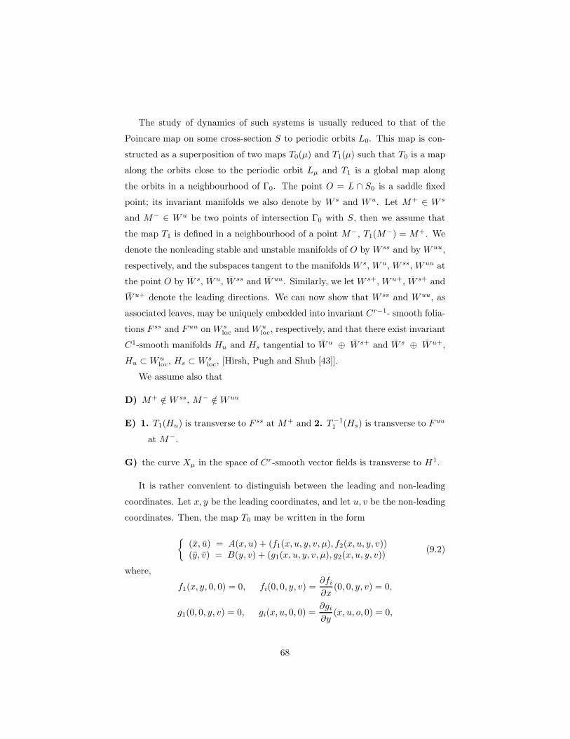
The study of dynamics of such systems is usually reduced to that of the

Poincare map on some cross-section S to periodic orbits L0. This map is con-

structed as a superposition of two maps T0(µ) and T1(µ) such that T0 is a map

along the orbits close to the periodic orbit Lµ and T1 is a global map along

the orbits in a neighbourhood of Γ0. The point O = L ∩ S0 is a saddle fixed

point; its invariant manifolds we also denote by W s and Wu. Let M+ ∈ W s

and M− ∈ Wu be two points of intersection Γ0 with S, then we assume that

the map T1 is defined in a neighbourhood of a point M−, T1(M−) = M+. We

denote the nonleading stable and unstable manifolds of O by W ss and by Wuu,

respectively, and the subspaces tangent to the manifoldsW s, Wu, W ss, Wuu at

the point O by W s, Wu, W ss and Wuu. Similarly, we let W s+, Wu+, W s+ and

Wu+ denote the leading directions. We can now show that W ss and Wuu, as

associated leaves, may be uniquely embedded into invariant Cr−1- smooth folia-

tions F ss and Fuu onW sloc andW

uloc, respectively, and that there exist invariant

C1-smooth manifolds Hu and Hs tangential to Wu ⊕ W s+ and W s ⊕ Wu+,

Hu ⊂Wuloc, Hs ⊂W s

loc, [Hirsh, Pugh and Shub [43]].

We assume also that

D) M+ /∈ W ss, M− /∈Wuu

E) 1. T1(Hu) is transverse to Fss at M+ and 2. T−1

1 (Hs) is transverse to Fuu

at M−.

G) the curve Xµ in the space of Cr-smooth vector fields is transverse to H1.

It is rather convenient to distinguish between the leading and non-leading

coordinates. Let x, y be the leading coordinates, and let u, v be the non-leading

coordinates. Then, the map T0 may be written in the form

(x, u) = A(x, u) + (f1(x, u, y, v, µ), f2(x, u, y, v))(y, v) = B(y, v) + (g1(x, u, y, v, µ), g2(x, u, y, v))

(9.2)

where,

f1(x, y, 0, 0) = 0, fi(0, 0, y, v) =∂fi∂x

(0, 0, y, v) = 0,

g1(0, 0, y, v) = 0, gi(x, u, 0, 0) =∂gi∂y

(x, u, o, 0) = 0,

68

and fi and g - Cr−1 are smooth functions.

Let Π0 and Π1 be sufficiently small neighbourhoods of the pointsM+(x+, u+, 0, 0)

and M−(0, 0, y−, v−):

Π0 = (x0, u0, y0, v0)/‖(x0 − x+, u0 − u+)‖ ≤ ǫ0, ‖(y0, v0)‖ ≤ ǫ0 ,

Π1 = (x1, u1, y1, v1)/‖(x1, u1)‖ ≤ ǫ0, ‖(y1 − y−, v1 − v−)‖ ≤ ǫ0 .(9.3)

The map T ′ : Π0 7→ Π1 along the trajectories of the system in a neighbourhood

of Lµ is defined on σ0 ⊂ Π0, where σ0 consists of a countable set of non-crossing

”strips” σ0n and

⋃∞n=k T

n0 σ

0n = T ′σ0 ⊂ Π1, where k stands for a number

(maximal) of the iterations under which the map of the strips is defined; k

depends on the size of the chosen neighbourhood. Denote σ1n = T n0 σ

0n.

Introduce the coordinates (xi, ui, yi, vi) in neighbourhoods Πi. The map

T n0 σ0n can be then written in a cross-form

x1 = An1x0 + ψ1(x0, u0, y1, v1)u1 = An2u0 + ψ2(x0, u0, y1, v1)y0 = B−n

1 y1 + ψ3(x0, u0, y1, v1)v0 = B−n

2 v1 + ψ4(x0, u0, y1, v1)

(9.4)

where ‖ψi‖Cr−2 ≤ λn, i = 1, 2, ‖ϕj‖Cr−2 ≤ γ−n, j = 3, 4, λ > λ >

max|λi|, |λ/γ|, γ < γ < min|γj|, γ2, ‖A2‖ < λ−1,∥∥B−1

2

∥∥ < γ−1, and

in the case A1) An1 = λn;

In the case A2) An1 = λnE(nϕ), where E(nϕ) =

(cos(nϕ) − sin(nϕ)sin(nϕ) cos(nϕ)

)

;

In the case A3) B−n γ−n;

In the case A4) N−n1 = λnE(−nψ), whereE(nψ) =

(cos(nψ) − sin(nψ)sin(nψ) cos(nψ)

)

.

Taking into account the conditions C) - F) the map T1 : S 7→ S along

orbits of the system Xµ in a neighbourhood Γ0 recast as :

x0 − x+ = F x(x1, u1, y1 − y−, v0),u0 − u+ = Fu(x1, u1, y1 − y−, v0),

y0 = G(x1, u1, y1 − y−, v0),v1 − v− = H(x1, u1, y1 − y−, v0),

(9.5)

where F x, Fu, G, H Cr are smooth functions, ∂Fx

∂y1(0, 0, 0, 0, 0) = b 6= 0,

G(x1, u1, y1−y−, v0) = D(x1, u1, y1−y−, v0)·(y1−y−ψ)2+C(x1, u1, v0), (9.6)

69

D(0, 0, 0, 0) = d, ψ(0, 0, 0) = 0, C(0, 0, 0) = 0, ∂C∂x (0, 0, 0) = c 6= 0 and y1−y− =

ψ(x1, u1, v0) is a solution of the equation ∂G∂y1

(x1, u1, y1 − y−, v0) = 0.

As we stated above, the homoclinic trajectories may be three types: we

partition the systems satisfying (A)-(E) into three subclasses. The systems of

the first class are defined by the condition that if σ < 1, then γ is real and

positive and d < 0, and if σ > 1, then λ is real and positive and dc > 0. The

second class consists of systems with real and positive γ and λ such that d > 0

and c < 0. All the rest go into the third class.

We consider a small neighbourhood U of the contour L ∪ Γ. Let N be the

set of trajectories of the system X that lie entirely within N .

Theorem 9.2 For systems of the first class, N = L,Γ. For systems of

the second class N is equivalent to the suspension over the Bernoulli shift

on three symbols 0, 1, 2 in which the trajectories · · · 0 · · · 010 · · ·0 · · · and

· · · 0 · · · 020 · · ·0 · · · are identified.

For systems of the third class, N also has nontrivial hyperbolic subsets, bu

they do not in general exhaust all of N . Moreover, under the motion along the

surface B13 of systems of the third class the structure of the set N varies con-

tinuously. The main reason for this is the presence of moduli of Ω-equivalence.

The multipliers λ1 and γj such that |λi| = λ and |γj | = γ are said to be leading

and the remainder are non-leading. Let ps denote the number of the leading λi

and let pu denote the number of leading γj . We will then say that X has type

(ps, pu). We also set θ = −l ln λ/ ln γ.

Theorem 9.3 Let X1, X2 ∈ B13 . Then for Ω-equivalence 19 of X1 and X2 it

is necessary that θ1 = θ2 in the case of systems of type (1,1); that θ1 = θ2 and

ϕ1 = ϕ2 for systems of type (2,1); that θ1 = θ2 and ψ1 = ψ2 for systems of

type (1,2); and for systems of type (2,2): ϕ1 = ϕ2 and ψ1 = ψ2, and also θ1 =

θ2, except, perhaps, for the case ϕ1 = ϕ2 = ψ1 = ψ2 ∈ 2π/3, π/2, 2π/5, π/3.

The quantities ψ, ϕ and θ are the fundamental moduli in the sense that

they are defined everywhere on B13 . If ψ/2π, ϕ2π, or θ is irrational, then there

19We talk about Ω-equivalence via a homeomorphism that is homotopic to the identity inU .

70

also exist other moduli, for example, analogous to the quantity τ introduced in

[Gonchenko and Shilnikov [28, 29, 30]]. Moreover, we have

Theorem 9.4 In B13 there is a dense set B∗ of systems that have a countable

number of saddle periodic orbits with structurally unstable homoclinic curves of

the third class.

For systems from B∗ the quantities θ computed for the corresponding saddle

periodic orbits are moduli of Ω-equivalence (theorem 9.3). Thus, we have a

theorem which generalizes a result from [33, 34] to the higher-dimensional case.

Theorem 9.5 In B13 the systems with a countable number of moduli of Ω-

equivalence are dense.

We note that if the Ω-moduli are chosen as parameters, as they change,

bifurcations of the non-wandering trajectories must occur — periodic orbits,

homoclinic orbits, etc. Here, the presence of a countable number of moduli lead

to infinitely degenerate bifurcations. Thus, we have

Theorem 9.6 In B13 the systems with a countable number of structurally un-

stable homoclinic curves of arbitrary orders of tangency and with a countable

number of structurally unstable periodic orbits, both with multipliers ρ = 1 and

with ρ = −1, of arbitrary orders of degeneracy are dense.

Let X be a system from B1 (not necessarily of the third class). We consider

a Cr-smooth finite-parameter family Xµ, transversally intersecting B1 at X for

µ = 0. We will call the open sets in the space of dynamical systems, in which the

systems with structurally unstable homoclinic curves are dense, the Newhouse

regions. From Gonchenko, Shilnikov and Turaev [35, 37] we obtain

Theorem 9.7 There exists a sequence of open sets ∆i accumulating to µ = 0

such that Xµ for µ ∈ ∆i lie in the Newhouse region, and the values of µ for

which the periodic orbit Lµ has a structurally unstable homoclinic curve of the

third class are dense in ∆i.

From the two last theorems we get

71

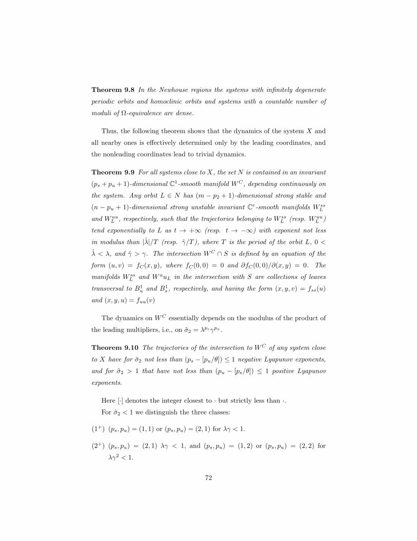
Theorem 9.8 In the Newhouse regions the systems with infinitely degenerate

periodic orbits and homoclinic orbits and systems with a countable number of

moduli of Ω-equivalence are dense.

Thus, the following theorem shows that the dynamics of the system X and

all nearby ones is effectively determined only by the leading coordinates, and

the nonleading coordinates lead to trivial dynamics.

Theorem 9.9 For all systems close to X, the set N is contained in an invariant

(ps + pu + 1)-dimensional C1-smooth manifold WC , depending continuously on

the system. Any orbit L ∈ N has (m − p2 + 1)-dimensional strong stable and

(n − pu + 1)-dimensional strong unstable invariant Cr-smooth manifolds W ssL

and WuuL , respectively, such that the trajectories belonging to W ss

L (resp. WuuL )

tend exponentially to L as t → +∞ (resp. t → −∞) with exponent not less

in modulus than |λ|/T (resp. γ/T ), where T is the period of the orbit L, 0 <

λ < λ, and γ > γ. The intersection WC ∩ S is defined by an equation of the

form (u, v) = fC(x, y), where fC(0, 0) = 0 and ∂fC(0, 0)/∂(x, y) = 0. The

manifolds W ssL and WuuL in the intersection with S are collections of leaves

transversal to B1u and B1

s , respectively, and having the form (x, y, v) = fss(u)

and (x, y, u) = fuu(v)

The dynamics on WC essentially depends on the modulus of the product of

the leading multipliers, i.e., on σ2 = λpsγpu .

Theorem 9.10 The trajectories of the intersection to WC of any system close

to X have for σ2 not less than (ps − [pu/θ]) ≤ 1 negative Lyapunov exponents,

and for σ2 > 1 that have not less than (pu − [ps/θ]) ≤ 1 positive Lyapunov

exponents.

Here [·] denotes the integer closest to · but strictly less than ·.For σ2 < 1 we distinguish the three classes:

(1+) (ps, pu) = (1, 1) or (ps, pu) = (2, 1) for λγ < 1.

(2+) (ps, pu) = (2, 1) λγ < 1, and (ps, pu) = (1, 2) or (ps, pu) = (2, 2) for

λγ2 < 1.

72

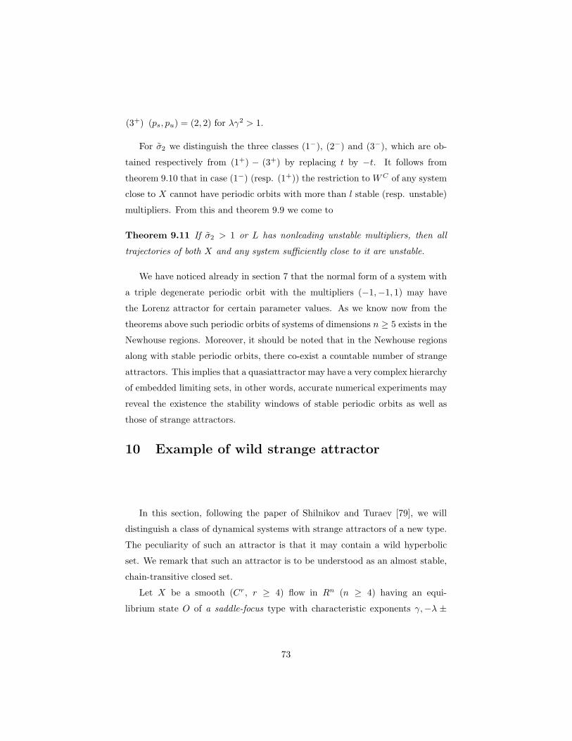
(3+) (ps, pu) = (2, 2) for λγ2 > 1.

For σ2 we distinguish the three classes (1−), (2−) and (3−), which are ob-

tained respectively from (1+) − (3+) by replacing t by −t. It follows from

theorem 9.10 that in case (1−) (resp. (1+)) the restriction toWC of any system

close to X cannot have periodic orbits with more than l stable (resp. unstable)

multipliers. From this and theorem 9.9 we come to

Theorem 9.11 If σ2 > 1 or L has nonleading unstable multipliers, then all

trajectories of both X and any system sufficiently close to it are unstable.

We have noticed already in section 7 that the normal form of a system with

a triple degenerate periodic orbit with the multipliers (−1,−1, 1) may have

the Lorenz attractor for certain parameter values. As we know now from the

theorems above such periodic orbits of systems of dimensions n ≥ 5 exists in the

Newhouse regions. Moreover, it should be noted that in the Newhouse regions

along with stable periodic orbits, there co-exist a countable number of strange

attractors. This implies that a quasiattractor may have a very complex hierarchy

of embedded limiting sets, in other words, accurate numerical experiments may

reveal the existence the stability windows of stable periodic orbits as well as

those of strange attractors.

10 Example of wild strange attractor

In this section, following the paper of Shilnikov and Turaev [79], we will

distinguish a class of dynamical systems with strange attractors of a new type.

The peculiarity of such an attractor is that it may contain a wild hyperbolic

set. We remark that such an attractor is to be understood as an almost stable,

chain-transitive closed set.

Let X be a smooth (Cr , r ≥ 4) flow in Rn (n ≥ 4) having an equi-

librium state O of a saddle-focus type with characteristic exponents γ,−λ ±

73

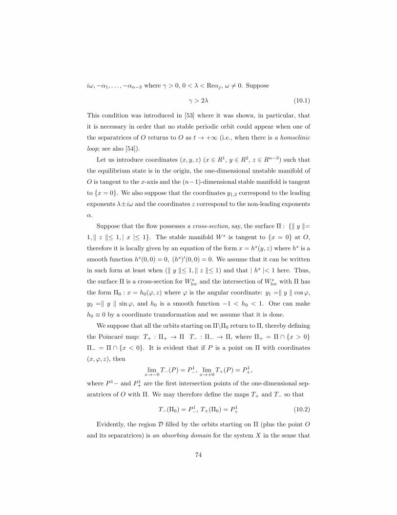
iω,−α1, . . . ,−αn−3 where γ > 0, 0 < λ < Reαj , ω 6= 0. Suppose

γ > 2λ (10.1)

This condition was introduced in [53] where it was shown, in particular, that

it is necessary in order that no stable periodic orbit could appear when one of

the separatrices of O returns to O as t→ +∞ (i.e., when there is a homoclinic

loop; see also [54]).

Let us introduce coordinates (x, y, z) (x ∈ R1, y ∈ R2, z ∈ Rn−3) such that

the equilibrium state is in the origin, the one-dimensional unstable manifold of

O is tangent to the x-axis and the (n−1)-dimensional stable manifold is tangent

to x = 0. We also suppose that the coordinates y1,2 correspond to the leading

exponents λ±iω and the coordinates z correspond to the non-leading exponents

α.

Suppose that the flow possesses a cross-section, say, the surface Π : ‖ y ‖=1, ‖ z ‖≤ 1, | x |≤ 1. The stable manifold W s is tangent to x = 0 at O,

therefore it is locally given by an equation of the form x = hs(y, z) where hs is a

smooth function hs(0, 0) = 0, (hs)′(0, 0) = 0. We assume that it can be written

in such form at least when (‖ y ‖≤ 1, ‖ z ‖≤ 1) and that | hs |< 1 here. Thus,

the surface Π is a cross-section for W sloc and the intersection of W s

loc with Π has

the form Π0 : x = h0(ϕ, z) where ϕ is the angular coordinate: y1 =‖ y ‖ cosϕ,y2 =‖ y ‖ sinϕ, and h0 is a smooth function −1 < h0 < 1. One can make

h0 ≡ 0 by a coordinate transformation and we assume that it is done.

We suppose that all the orbits starting on Π\Π0 return to Π, thereby defining

the Poincare map: T+ : Π+ → Π T− : Π− → Π, where Π+ = Π ∩ x > 0Π− = Π ∩ x < 0. It is evident that if P is a point on Π with coordinates

(x, ϕ, z), then

limx→−0

T−(P ) = P 1−, lim

x→+0T+(P ) = P 1

+,

where P 1− and P 1+ are the first intersection points of the one-dimensional sep-

aratrices of O with Π. We may therefore define the maps T+ and T− so that

T−(Π0) = P 1−, T+(Π0) = P 1

+ (10.2)

Evidently, the region D filled by the orbits starting on Π (plus the point O

and its separatrices) is an absorbing domain for the system X in the sense that

74

the orbits starting in ∂D enter D and stay there for all positive values of time

t. By construction, the region D is the cylinder ‖ y ‖≤ 1, ‖ z ‖≤ 1, | x |≤ 1with two glued handles surrounding the separatrices (Fig.9.1).

We suppose that the (semi)flow is pseudohyperbolic in D. It is convenient forus to give this notion a sense more strong than it is usually done [43]. Namely,

we propose the following

Definition. A semiflow is called pseudohyperbolic if the following two condi-

tions hold:

A At each point of the phase space, the tangent space is uniquely decomposed

(and this decomposition is invariant with respect to the linearized semiflow)

into a direct sum of two subspaces N1 and N2 (continuously depending on

the point) such that the maximal Lyapunov exponent in N1 is strictly less

than the minimal Lyapunov exponent in N2: at each point M , for any

vectors u ∈ N1(M) and v ∈ N2(M)

lim supt→+∞

1

tln‖ut‖‖u‖ < lim inf

t→+∞

1

tln‖vt‖‖v‖

where ut and vt denote the shift of the vectors u and v by the semiflow

linearized along the orbit of the point M ;

B The linearized flow restricted on N2 is volume expanding:

Vt ≥ const · eσtV0

with some σ > 0; here, V0 is the volume of any region in N2 and Vt is the

volume of the shift of this region by the linearized semiflow.

The additional condition B is new here and it prevents of appearance of

stable periodic orbits. Generally, our definition includes the case where the

maximal Lyapunov exponent in N1 is non-negative everywhere. In that case,

according to condition A, the linearized semiflow is expanding in N2 and condi-

tion B is satisfied trivially. In the present paper we consider the opposite case

where the linearized semiflow is exponentially contracting in N1, so condition B

is essential here.

75

Note that the property of pseudohyperbolicity is stable with respect to small

smooth perturbation of the system: according to [43] the invariant decomposi-

tion of the tangent space is not destroyed by small perturbations and the spaces

N1 and N2 depend continuously on the system. Hereat, the property of volume

expansion in N2 is also stable with respect to small perturbations.

Our definition is quite broad; it embraces, in particular, hyperbolic flows for

which one may assume (N1, N2) = (Ns, Nu⊕N0) or (N1, N2) = (Ns⊕N0, Nu)

where Ns and Nu are, respectively, the stable and unstable invariant subspaces

and N0 is a one-dimensional invariant subspace spanned by the phase velocity

vector. The geometrical Lorenz model from [6, 7] or [40] belongs also to this

class: here N1 is tangent to the contracting invariant foliation of codimension

two and the expansion of areas in a two-dimensional subspace N2 is provided

by the property that the Poincare map is expanding in a direction transverse

to the contracting foliation.

In the present paper we assume that N1 has codimension three: dimN1 =

n − 3 and dimN2 = 3 and that the linearized flow (at t ≥ 0) is exponentially

contracting on N1. Condition A means here that if for vectors of N2 there is a

contraction, it has to be weaker than those on N1. To stress the last statement,

we will call N1 the strong stable subspace and N2 the center subspace and will

denote them as Nss and N c respectively.

We also assume that the coordinates (x, y, z) in Rn are such that at each

point of D the space Nss has a non-zero projection onto the coordinate space

z, and N c has a non-zero projection onto the coordinate space (x, y).

Note that our pseudohyperbolicity conditions are satisfied at the point O

from the very beginning: the space Nss coincides here with the coordinate

space z, and N c coincides with the space (x, y); it is condition (10.1) which

guarantees the expansion of volumes in the invariant subspace (x, y). The pseu-

dohyperbolicity of the linearized flow is automatically inherited by the orbits

in a small neighborhood of O. Actually, we require that this property would

extend into the non-small neighborhood D of O.

According to [43], the exponential contraction in Nss implies the existence of

an invariant contracting foliation N ss with Cr-smooth leaves which are tangent

76

to Nss. As in [7], one can show that the foliation is absolutely continuous. After

a factorization along the leaves, the regionD becomes a branched manifold (since

D is bounded and the quotient-semiflow expands volumes it follows evidently

that the orbits of the quotient-semiflow must be glued on some surfaces in order

to be bounded; cf.[40]).

The property of pseudohyperbolicity is naturally inherited by the Poincare

map T ≡ (T+, T−) on the cross-section Π: here, we have:

A∗ There exists a foliation with smooth leaves of the form (x, ϕ) = h(z) |−1≤z≤1,

where the derivative h′(z) is uniformly bounded, which possesses the fol-

lowing properties: the foliation is invariant in the sense that if l is a leaf,

then T−1+ (l∩T+(Π+∪Π0)) and T

−1− (l∩T−(Π−∪Π0)) are also leaves of the

foliation (if they are not empty sets); the foliation is absolutely continuous

in the sense that the projection along the leaves from one two-dimensional

transversal to another increases or decreases the area in a finite number of

times and the coefficients of expansion or contraction of areas are bounded

away from zero and infinity; the foliation is contracting in the sense that

if two points belong to one leaf, then the distance between the iterations

of the points with the map T tends to zero exponentially;

B∗ The quotient maps T+ and T− are area-expanding.

The fulfillment of conditions A∗, B∗ and relation (10.2) is sufficient for

theorems 10.1-?? below to be valid. As in [7], one can find sufficient conditions

for the fulfillment of A∗ and B∗.

Lemma 10.1 . Let us write the map T as

(x, ϕ) = g(x, ϕ, z), z = f(x, ϕ, z),

where f and g are functions smooth at x 6= 0 and discontinuous at x = 0:

limx→−0

(g, f) = (x−, ϕ−, z−) ≡ P 1−, lim

x→+0(g, f) = (x+, ϕ+, z+) ≡ P 1

+ .

Let

det∂g

∂(x, ϕ)6= 0 . (10.3)

77

Denote

A = ∂f∂z −

∂f∂(x,ϕ)

(∂g

∂(x,ϕ)

)−1∂g∂z , B = ∂f

∂(x,ϕ)

(∂g

∂(x,ϕ)

)−1

C =(

∂g∂(x,ϕ)

)−1∂g∂z , D =

(∂g

∂(x,ϕ)

)−1

.

If

limx→0

C = 0, limx→0‖ A ‖ ‖ D ‖= 0 (10.4)

supP∈Π\Π0

√

‖ A ‖ ‖ D ‖+√

supP∈Π\Π0

‖ B ‖ supP∈Π\Π0

‖ C ‖ < 1, (10.5)

then the map has a continuous invariant foliation with smooth leaves of the

form (x, ϕ) = h(z) |−1≤z≤1 where the derivative h′(z) is uniformly bounded. If,

additionally,

supP∈Π\Π0

‖ A ‖ +√

supP∈Π\Π0

‖ B ‖ supP∈Π\Π0

‖ C ‖ < 1, (10.6)

then the foliation is contracting and if, moreover, for some β > 0

the functions A | x |−β , D | x |β, B, C are uniformly bounded andHolder continuous,

and∂ ln det D

∂zand

∂ ln det D

∂(x, ϕ)D | x |β are uniformly bounded,

(10.7)

then the foliation is absolutely continuous. The additional condition

supP∈Π\Π0

√det D +

√

supP∈Π\Π0

‖ B ‖ supP∈Π\Π0

‖ C ‖ < 1 (10.8)

guarantees that the quotient map T expands areas.

It follows from [53, 54] that in the case where the equilibrium state is a

saddle-focus, the Poincare map near Π0 = Π ∩W s is written in the following

form under some appropriate choice of the coordinates.

(x, ϕ) = Q±(Y, Z), z = R±(Y, Z). (10.9)

Here

Y =| x |ρ(

cos(Ω ln | x | +ϕ) sin(Ω ln | x | +ϕ)− sin(Ω ln | x | +ϕ) cos(Ω ln | x | +ϕ)

)

+Ψ1(x, ϕ, z),

Z = Ψ2(x, ϕ, z),(10.10)

78

where ρ = λ/γ < 1/2 (see (10.1)), Ω = ω/γ and, for some η > ρ,

‖ ∂p+|q|Ψi∂xp∂(ϕ, z)q

‖= O(| x |η−p), 0 ≤ p+ | q |≤ r − 2 ; (10.11)

the functions Q±, R± in (10.9) (“+” corresponds to x > 0 - the map T+, “-”

corresponds to x < 0 - the map T−) are smooth functions in a neighborhood of

(Y, Z) = 0 for which the Taylor expansion can be written down

Q± = (x±, ϕ±) + a±Y + b±Z + . . . , R± = z± + c±Y + d±Z + . . . (10.12)

It is seen from (10.9)-(10.12) that if O is a saddle-focus satisfying (10.1), then

if a+ 6= 0 and a− 6= 0, the map T satisfies conditions (10.4) and (10.7) with

β ∈ (ρ, η). Furthermore, analogues of conditions (10.3),(10.5),(10.6), (10.8) are

fulfilled where the supremum should be taken not over | x |≤ 1 but it is taken

over small x. The map (10.9),(10.10),(10.12) is easily continued onto the whole

cross-section Π so that the conditions of the lemma were fulfilled completely.

An example is given by the map

x = 0.9 | x |ρ cos(ln | x | +ϕ),

ϕ = 3 | x |ρ sin(ln | x | +ϕ),

z = (0.5 + 0.1z | x |η) sign x

(10.13)

where 0.4 = ρ < η

As stated above, the expansion of volumes by the quotient-semiflow restricts

the possible types of limit behavior of orbits. Thus, for instance, in D there may

be no stable periodic orbits. Moreover, any orbit in D has a positive maximal

Lyapunov exponent. Therefore, one must speak about a strange attractor in

this case.

Beforehand, we recall some definitions and simple facts from topological

dynamics. Let XtP be the time-t shift of a point P by the flow X . For given ε >

0 and τ > 0 let us define as an (ε, τ)-orbit as a sequence of points P1, P2, . . . , Pk

such that Pi+1 is at a distance less than ε from XtPi for some t > τ . A point Q

will be called (ε, τ)-attainable from P if there exists an (ε, τ)-orbit connecting

P and Q; and it will be called attainable from P if, for some τ > 0, it is

(ε, τ)-attainable from P for any ε (this definition, obviously, does not depend

79

on the choice of τ > 0). A set C is attainable from P if it contains a point

attainable from P . A point P is called chain-recurrent if it is attainable from

XtP for any t. A compact invariant set C is called chain-transitive if for any

points P ∈ C and Q ∈ CC and for any ε > 0 and τ > 0 the set C contains an

(ε, τ)-orbit connecting P and Q. Clearly, all points of a chain-transitive set are

chain-recurrent.

A compact invariant set C is called orbitally stable, if for any its neighbor-

hood U there is a neighborhood V (C) ⊆ U such that the orbits starting in V

stay in U for all t ≥ 0. An orbitally stable set will be called completely stable

if for any its neighborhood U(C) there exist ε0 > 0, τ > 0 and a neighbor-

hood V (C) ⊆ U such that the (ε0, τ)-orbits starting in V never leave U . It is

known, that a set C is orbitally stable if and only if C =

∞⋂

j=1

Uj where Uj∞j=1

is a system of embedded open invariant (with respect to the forward flow) sets,

and C is completely stable if the sets Uj are not just invariant but they are

absorbing domains (i.e.; the orbits starting on ∂Uj enter inside Uj for a time

interval not greater than some τj ; it is clear in this situation that (ε, τ)-orbits

starting on ∂Uj lie always inside Uj if ε is sufficiently small and τ ≥ τj). Since

the maximal invariant set (the maximal attractor) which lies in any absorbing

domain is, evidently, asymptotically stable, it follows that any completely stable

set is either asymptotically stable or is an intersection of a countable number of

embedded closed invariant asymptotically stable sets.

Let us construct such an attractor of the system X and give an estimate

of the number of the connected components of the intersection of the attractor

with the cross-section Π.

Definition. We call the set A of the points attainable from the equilibrium

state O the attractor of the system X.

This definition is justified by the following theorem.

Theorem 10.1 The set A is chain-transitive, completely stable and attainable

from any point of the absorbing domain D.

The stability of A follows immediately from the definition: it is known that

for any initial point (and for the point O, in particular) the set of attainable

80

points is completely stable (the system of absorbing domains is given by the sets

of the points (εj , τ)-attainable from the initial point, with arbitrary εj → +0

and τ > 0).

To prove the rest of the theorem note that the following lemma is valid.

Lemma 10.2 Points asymptotic to O as t → +∞ are dense in D (in other

words, the stable manifold of O is dense in D).

Indeed, take an arbitrary point on Π and let U be a neighborhood of Π. If U

would not intersect with the pre-images of the surface Π0 =W sloc ∩ Π, then for

all i ≥ 0 the map T i |U is continuous and the areas of the projections of the

sets T iU onto z = 0 along the leaves of the invariant foliation would increase

exponentially (by virtue of property B∗), which contradicts the boundedness of

Π. Thus, the pre-images of Π0 (and these are the intersections of the stable

manifold of O with the cross-section Π) are dense in Π, which implies that the

stable manifold of O is dense in D.Lemma 10.2 implies immediately that O is attainable from any point of D.

In particular, for any two points P and Q in A, the point O is attainable from

P whereas Q is attainable from O according to the definition of A. Hence,

Q is attainable from P , and to prove the chain-transitivity of A it remains to

show that the (ε, τ)-orbits connecting P and Q can be chosen lying in A. This,however, follows from the complete stability of A: for any δ > 0, an (ε, τ)-orbit

connecting P and Q does not leave the δ-neighborhood of A if ε is sufficiently

small, whence this (ε, τ)-orbit may be approximated by an (ε′, τ)-orbit which

lies in A where ε′ may be greater than ε but, clearly, ε′ → 0 as ε→ 0, δ → 0.

Theorem 10.1 implies that A is the least completely stable subset of D: sinceany point belongs to a completely stable set together with all points attainable

from it, theorem 10.1 implies that any completely stable subset of D must

contain the point O and, consequently, the set A. Thus, A is the intersection

of all completely stable subsets of D.The next theorem shows that A is a unique chain-transitive and completely

stable set in D.

81

Theorem 10.2 If an orbitally stable subset of D contains points which do not

belong to A, it contains points which are not chain-recurrent.

Proof. Since the stable manifold of O is dense in D, any orbitally stable subset

of D contains the point O. Since any connected component of an orbitally stable

set is orbitally stable itself, we have that each of the components must contain

O whence there is only one component; i.e., any orbitally stable subset of D is

connected. Let C be such a set and suppose there is a point P ∈ C, P 6∈ A.Since A is completely stable, there exists an absorbing domain U which contains

A and does not contain P . The point O belongs to both A and C: we have

that C contains points both inside U and outside U . The set C is connected

and, hence, it must contain at least one point on ∂U . As we stated above, the

(ε, τ)-orbits starting on ∂U always lie inside U , at a finite distance from ∂U , if

ε is sufficiently small and τ is sufficiently large, which means that no point of

∂U is chain-recurrent.

The next theorem extends into the multi-dimensional case the result of item 1

of theorem 1.5 in [7] and gives a description of the decomposition into connected

components of the intersection of the attractor A with the cross-section Π; we

will use this in the proof of theorem 10.4 Let q > 1 be the area expansion factor

for the quotient map T : if V is a region in Π not intersecting Π0, then

S(TV ) > qS(V ), (10.14)

where S denotes the area of the projection of the region onto the surface z = 0along the leaves of the invariant foliation. According toB∗, q > 1. Besides, since

S(Π) = 2S(Π+) and TΠ+ ⊂ Π, we have S(TΠ+)/S(Π+) < 2, and therefore

1 < q < 2.

Let us denote the separatrices of O by Γ+ and Γ−, and let P±i be the con-

secutive points of intersection of Γ± with Π; these sequences may be infinite or

finite, the latter if the corresponding separatrix forms a homoclinic loop (returns

to O as t→ +∞).

82

Theorem 10.3 The number N of connected components of the set A ∩ Π is

finite and

2 ≤ N < 2 +| ln(q − 1) |

ln q. (10.15)

Each of the components contains at least one of the points P±i . Furthermore,

for some integers N+ ≥ 1, N− ≥ 1, N+ +N− = N , satisfying the inequality

q−N+ + q−N− > 1, (10.16)

the set A ∩ Π is represented in the form

A ∩ Π = A+1 ∪ · · · ∪ A+

N+∪ A−

1 ∪ · · · ∪ A−N

−

, (10.17)

where A+i and A−

i are the components containing the points P+i and P−

i respec-

tively. In this formula all the components A±i are different,

A+i ∩Π0 = ∅ i < N+, A−

i ∩ Π0 = ∅ i < N−,

A+N+∩ Π0 6= ∅, A−

N−

∩ Π0 6= ∅;(10.18)

and

T+[(A−N

−

∪ A+N+

) ∩ (Π+ ∪ Π0)] = A+1 , T−[(A−

N−

∪ A+N+

) ∩ (Π− ∪Π0)] = A−1 ,

A−i = T i−1A−

1 at i < N−, A+i = T i−1A+

1 at i < N+ ,(10.19)

(see Fig. 9.2).

Let us take a one-parameter family Xµ of systems of the kind under consid-

eration and assume that

a homoclinic loop of the saddle-focus O exists at µ = 0,

i.e., one of the separatrices (say, Γ+) returns to O as t→ +∞. In other words,

we assume that the family Xµ intersects, at µ = 0, a bifurcational surface filled

by systems with a homoclinic loop of the saddle-focus and we suppose that this

intersection is transverse. The transversality means that when µ varies, the loop

splits and if M is the number of the last point of intersection of the separatrix

Γ+ with the cross-section Π at µ = 0 (P+M ∈ Π0 at µ = 0), then the distance

between the point P+M and Π0 changes with a “non-zero velocity” when µ varies.

We choose the sign of µ so that P+M ∈ Π+ when µ > 0 (respectively, P+

M ∈ Π−

when µ < 0).

83

Theorem 10.4 There exists a sequence of intervals ∆i (accumulated at µ =

0) such that when µ ∈ ∆i, the attractor Aµ contains a wild set (non-trivial

transitive closed hyperbolic invariant set whose unstable manifold has points of

tangency with its stable manifold). Furthermore, for any µ∗ ∈ ∆i, for any

system Cr-close to a system X∗µ, its attractor A also contains the wild set.

As far as the general case is concerned when the separatrix of the point O

do not form the homoclinic loops, we note that as it follows from the density of

the stable manifold in D that the separatrix of the point O are non-wandering

trajectories. So we can suppose that they may be closed by small perturbations

of the system. A similar problem has already arozen in the case of the Lorenz

map but it was overcome (in Cr-topology) using certain specific properties of

the map. By now we have a rather important lemma of Hayashi [41] which

allows us to solve this problem. Hence the following statement is true

Statement The systems with a homoclinic loop to a saddle-focus are dense

in Cr-topology in the class of systems under consideration.

We have mentioned that the presence of structurally unstable (non-transverse)

homoclinic trajectories leads to non-trivial dynamics. Thus, using results [33,

37] we can conclude from theorem 10.4 that the systems whose attractors con-

tain structurally non-transverse homoclinic trajectories as well as structurally

unstable periodic orbits of high order of degeneracy are dense in the given re-

gions in the space of dynamical systems. In particular, the values of µ are dense

in the intervals ∆i for which an attractor of the system contain a periodic orbit

of the saddle-saddle type along with its three-dimensional unstable manifold.

For these parameter values, the topological dimension of such an attractor is

already not less than three. The latter implies that the given class of systems

is an example of hyperchaos.

Up to now we have not yet spoken about the statistical properties of the

attractors. This is necessary since all of the trajectories of the strange attractors

are unstable. Sinai [65] introduced the following notion of a stochastic attractor.

A stochastic attractor is an invariant closed set A in the phase space with the

following properties:

84

1. There exists a neighbourhood U , A ⊂ U , such that if x ∈ U , then dist(x(t), A)→0 as t→ +∞.

2. For any initial probability distribution P0 on A, its shift as t→ +∞ to an

invariant distribution P on A, independently of P0.

3. The probability distribution P is mixing, i.e., the autocorrelation function

tends to zero as t→∞.

It is known that on hyperbolic attractors (and even on non-trivial basis

sets) an invariant, “rather” physical measure, the so-called Bowen-Ruelle-Sinai

measure may be introduced. This allows one to prove that hyperbolic attractors

are stochastic in the sense above. This result is true for Lorenz-like attractors as

well [20]]. Both types of such attractors have a specific feature: the dimension of

the stable (unstable) manifolds of their trajectories (excluding the saddle point

at the origin in the case of the Lorenz attractor) is always the same, i.e., such

an attractor contain the trajectories of the same topological type. This is not

the case when we deal with the wild strange attractors since it may contain

co-existing hyperbolic trajectories of various types. This is a challenge for the

ergodic theory.

Acknowledgments

The author would like to thank L. Chua for useful discussions. He is also grateful

to A. Shilnikov for help in preparing this manuscript.

This work was supported in part by the Russian Foundation of Basic Re-

search 96-01001135 and by INTAS-93-0570.

85

References

[1] A.A.Andronov, E.A.Leontovich, I.E.Gordon and A.G.Maier [1971] The the-

ory of bifurcations of dynamical systems on a plane, Izrael program of sci-

entific translations, Izrael

[2] A.A.Andronov, E.A.Leontovich, I.E.Gordon and A.G.Maier [1973] The the-

ory of dynamical systems on a plane, Izrael program of scientific transla-

tions, Izrael

[3] A.A.Andronov and L.Pontryagin [1937] Systemes Grossiers, Dokl. Acad.

Nauk SSSR, 14, pp.247-251

[4] A.A.Andronov, E.A.Vitt and S.E.Khaikin [1966] Theory of oscillations,

Pergamon Press: Oxford

[5] V.S. Afraimovich, V.I.Arnold, Yu.S.Il’yashenko and L.P.Shilnikov [1989],

Bifurcation theory in Dynamical Systems V, Encyclopedia of Math. Sci-

ences, 5, Springer-Verlag

[6] V.S.Afraimovich, V.V.Bykov and L.P.Shilnikov [1977], On the appearance

and structure of Lorenz attractor, DAN SSSR, 234, pp.336-339

[7] V.S.Afraimovich, V.V.Bykov and L.P.Shilnikov [1983], On the structurally

unstable attracting limit sets of Lorenz attractor type, Tran. Moscow Math.

Soc., 2, pp.153-215

[8] V.S.Afraimovich and L.P.Shilnikov [1973], On critical sets of Morse-Smale

systems. Trudy Moskov. Mat. Obsh. 28 pp.181-214; English transl. in

Trans. Moscow Math. Soc. 28 [1973].

[9] V.S.Afraimovich and L.P.Shilnikov [1974], On some global bifurcations con-

nected with disappearance of saddle-node fixed point, Dokl. Acad. Nauk

SSRR 219 pp.1981-1985

[10] V.S.Afraimovich and L.P.Shilnikov [1983], Strange attractors and quasi-

attractors in Nonlinear Dynamics and Turbulence eds. by G.I.Barenblatt,

G.Iooss and D.D.Joseph, Pitman, NY, pp.1-28

86

[11] D.Anosov [1967] Geodesic flows on compact Riemannian manifolds of neg-

ative curvature, Trudy Math. Inst. im. V.A.Steklova, 90 [in Russian]

[12] D.V.Anosov, S.Kh.Aronson, I.U.Bronshtein and V.Z.Grines [1985], Smooth

dynamical systems in Dynamical Systems, Encyclopedia of Math. Sciences,

1, Springer-Verlag

[13] D.V.Anosov and V.V.Solodov [1991], Hyperbolic sets in Dynamical systems

9, Encyclopedia of Math. Sciences, 66, Springer-Verlag

[14] S.Kh.Aronson and V.Z.Grines [1991], Cascades on surfaces in Dynamical

systems with hyperbolic behaviour. Dynamical Systems 9, Encyclopedia of

Math. Sciences, 66, Springer-Verlag

[15]

[16] M.Benedicks and L.Carleson [1991], The dynamics of the Henon map, Ann.

Math, 133(1), pp.73-169

[17] G.D.Birkhoff [1935], Nouvelles recherche sur les systemes dynamiques,

Memorie Pont Acad. Sci. Novi Lyncaei, 3(1), pp.85-216

[18] R.Bowen [1970], Markov partition for Axiom A diffeomorphisms, Amer. J.

Math., 92(3), pp.724-747

[19] R.Bowen [1973], Symbolic dynamics for hyperbolic flows, Amer. J. Math.,

95(2), pp.429-460

[20] L.A.Bunimovich and Ya.G.Sinai [1980] Stochasticity of an attractor in

the Lorenz model, in Nonlinear waves ed. A.V.Gaponov-Grekhov, Nauka,

pp.212-226, [in Russian]

[21] V.V.Bykov and A.L.Shilnikov (1992) On boundaries of the region of exis-

tence of the Lorenz attractor, Selecta Math. Sovietica, v.11[4], pp.375-382

[22] O.L.Chua [1993], Global unfolding of Chua’s circuit, IEICE Trans. Fund.

ECCS, 76-SA, pp.704-734

87

[23] W. de Melo and S.J. van Streen [1979] Diffeomorphisms on surfaced with

fonite number of moduli, Ergog. Th. and Dynam. Systems, 7, pp.415-462

[24] A.Donjoy [1932] Sur les courbes defines par les equationa differentielles a

la surface du tore, J. Math, 17(IV), pp.333-375

[25] R.Devaney and Z.Nitecki [1979], Shift automorphism in the Henon map-

ping, Comm. Math. Phys., 67, pp.137-148.

[26] N.K.Gavrilov and L.P.Shilnikov [1972]. On three-dimensional dynamical

systems close to systems with a structurally unstable homoclinic curve.

Part 1, Math.USSR Sb., 17 (1972), pp.467-485 ; [1973] Part 2, Math.USSR

Sb, 19, pp.139-156.

[27] S.V.Gonchenko. Moduli of Ω-conjugacy of two-dimensional diffeomor-

phisms with a structurally unstable heteroclinic cycle. Matemat. sbornik,

187 (1996), No. 9, pp. 3-25, in Russian.

[28] S.V.Gonchenko and L.P.Shilnikov [1986], On dynamical systems with struc-

turally unstable homoclinic curves, Soviet Math. Dokl., 33(1), pp.234-238.

[29] S.V.Gonchenko and L.P.Shilnikov [1987], Arithmetic properties of topologi-

cal invariants of systems with a structurally unstable homoclinic trajectory,

Ukrainian Math.J., 39(1), pp.21-28.

[30] S.V.Gonchenko and L.P.Shilnikov [1990], Invariants of Ω-conjugacy of dif-

feomorphisms with a structurally unstable homoclinic trajectory, Ukrainian

Math.J., 42(2), pp.134-140.

[31] S.V.Gonchenko and L.P.Shilnikov [1993], On moduli of systems with a

structurally unstable homoclinic Poincare curve. Russian Acad. Sci. Izv.

Math. 41(3), 417-445.

[32] S.V.Gonchenko and L.P.Shilnikov. Geometrical properties of 2D-

diffeomorphisms with a structurally unstable homoclinic orbit. Int. J. Bi-

furcation and Chaos, 5 (1995), No.3, pp.21-28.

88

[33] S.V.Gonchenko, L.P.Shilnikov and D.V.Turaev [1992], On models with a

structurally unstable homoclinic Poincare curve, Sov. Math.Dokl., v.44[2],

pp.422-426

[34] S.V.Gonchenko, L.P.Shilnikov and D.V.Turaev [1993], On models with non-

rough Poincare homoclinic curves, Physica D, v.62, pp.1-14

[35] S.V.Gonchenko, D.V.Turaev and L.P.Shilnikov [1993], Dynamical phenom-

ena in multi-dimensional systems with a structurally unstable homoclinic

Poincare curve. Russian Acad. Sci. Dokl. Math., 47(3), pp.410-415.

[36] S.V.Gonchenko, D.V.Turaev and L.P.Shilnikov [1993], On the existence

of Newhouse domains in a neighborhood of systems with a structurally

unstable Poincare homoclinic curve (the higher-dimensional case). Russian

Acad. Sci. Dokl. Math. 47(2), pp.268-273.

[37] S.V.Gonchenko, L.P.Shilnikov and D.V.Turaev [1996] Dynamical phenom-

ena in systems with structurally unstable Poincare homoclinic orbits. In-

terdisc. J. CHAOS, 6(1), pp. 1-17.

[38] S.V.Gonchenko, L.P.Shilnikov and D.V.Turaev [1997], On the Newhose re-

gions of two-dimensional diffeomorphisms close to those with a structurally

unstable contour Trudy Steklov Mat. Inst., to be published

[39] J.Guckenheimer [1970], Endomorphisms of Riemann sphere, Global Anal-

ysis, Proc. Symp. Pure Math., —Providence, R.I. Amer. Math. Soc., 14,

pp.95-103.

[40] J.Guckenheimer and R.F.Williams [1979], Structural stability of Lorenz

attractors, Publ. Math. IHES, 50, pp.59-72

[41] S.Hayashi, On the solution of C1-stability conjecture for flow, Preprint

[42] , M.Henon [1976], A two-dimensional mapping with a strange attractor,

Comm. Math. Phys, 50, pp.69-77

[43] M. Hirsh, C.Pigh and M. Shub [1977], Invariant manifolds, Lecture Notes

in Math. Springer-Verlag,

89

[44] E.N.Lorenz [1963] Deterministic non-periodic flow, J. Atmos. Sci., 20,

pp.130-141

[45] R.N.Madan (Editor) [1993] Chua’s circuit: A paradigm for chaos, World

Sci. Series on Nonlinear Science, Ser. B, Vol.1 (Wold Sci, Singapore)

[46] R.Mane [1982] An orgodic closing lemma, Ann. Math, 116(2), pp.503-540

[47] V.K.Melnikov [1963], On stability of center periodically perturbated, Trudy

Mosc. Mat. Ob., 12, pp.3-52 [in Russian]

[48] J.Milnor and R.Thurston [1977] On iterated maps of the interval I ans II.

Unpublished notes, Prinseton University Press: Princeton

[49] S.Newhouse [1974], Diffeomorphisms with infinitely many sinks. Topology,

13, pp. 9-18.

[50] S.Newhouse [1979], The abundance of wild hyperbolic sets and nonsmooth

stable sets for diffeomorphisms.Publ. Math. I.H.E.S. 50, pp.101-151.

[51] S. Newhouse and J. Palis. Cycles and bifurcation theory. Asterisque. 31

(1976), 44-140.

[52] V.I.Oseledec [1968] A miltiplicative ergodic theorem: Lyapunov character-

istic numbers, Trans. Moscow Math. Soc., 19, pp.197-231

[53] I.M.Ovsyannikov and L.P.Shilnikov [1986] On systems with a saddle-focus

homoclinic curve, Mat. Sbornik, 58, pp.557-574; English translation in

Math. USSR Sb. 58, pp.557-574 [1987].

[54] I.M.Ovsyannikov and L.P.Shilnikov [1991] Systems with a homoclinic curve

of multidimensional saddle-focus type, and spiral chaos Mat. Sb. 182,

pp.1043-1073; English translation in Math. USSR Sb. 73, pp. 415-443

[1992].

[55] J.Palis [1978], A differentiable invariant of topological conjugacies and mod-

uli of stability, Asterisque, 51, pp. 335-346.

90

[56] M.M.Peixoto [1962] Structural stability on two-dimensional manifolds,

Topology, 1, pp.101-120

[57] H.Poincare [1899] Les Methodes nouvelles de la Mecanique celeste, 3, Paris

[58] R.Plykin (1974) Sources and sinks of A-diffeomorphism of surfaces, Math.

Sbornik, v.94, pp.243-264

[59] R.Plykin, E.A.Sataev and C.V.Shlyachkov [1991], Strange attractors in Dy-

namical systems 9, Encyclopedia of Math. Sciences, 66, Springer-Verlag

[60] C.Robinson [1981], Differentiability of the stable foliation for the model

Lorenz equations, Lect. Not. in Math., 898, p.302-315

[61] C.Robinson [1989], Homoclinic bifurcation to a transitive attractor of

Lorenz type, Nonlinearity, 2(4), pp.495-518

[62] M.Rychlik [1990], Lorenz attractor through Shilnikov type bifurcation, Er-

god. Theory and Dyn. Syst., 10(4), 793-821

[63] M.V.Shashkov and L.P.Shilnikov L.P. [1994], On existence of a smooth in-

variant foliation for maps of the Lorenz type, Differential Equations, 30(4),

pp.586-595 [in Russian]

[64] Ya.G.Sinai [1968], Markov partitions and U-diffeomorphisms, Fun. Anal.,

2(1), pp.64-89

[65] Ya.G.Sinai [1980] Stochasticity of dynamical systems attractor in the

Lorenz model, in Nonlinear waves ed. A.V.Gaponov-Grekhov, Nauka,

pp.192-212

[66] S.Smale [1963] Diffeomorphisms with many periodic point. in Diff. and

Comb.Topology ed. by S.Cairus, Princeton Univ Press, Princeton, pp.63-86

[67] S.Smale [1967] Differentiable dynamical systems,Bulletin of Amer. Math.

Soc., 73, pp.747-817

[68] A.L.Shilnikov [1986], Bifurcations and chaos in the Shimizu-Marioka sys-

tem [In Russian], inMethods and qualitative theory of differential equations,

91

Gorky State University, pp.180-193 [English translation in Selecta Mathe-

matica Sovietica 10 pp.105-117, [1991]]

[69] A.L.Shilnikov [1993], On bifurcations of the Lorenz attractor in the

Shimizu-Marioka system, Physica D62 pp.338-346

[70] A.L.Shilnikov, L.P.Shilnikov and D.V.Turaev [1993], Normal forms and

Lorenz attractors, Int. J. Bifurcations and Chaos, 1(4), pp.1123-1139

[71] L.P.Shilnikov [1965] A case of the existence of a countable set of periodic

motions, Sov.Math.Dokl., 6, pp.163-166.

[72] L.P.Shilnikov [1969] On a new type of bifurcation of multi-dimensional

dynamical systems, Soviet Math. Dokl., 10, pp.1368-1371

[73] L.P.Shilnikov [1970] A contribution to the problem of the structure of an

extended neighbourhood of a rough state of saddle-focus type, Math.USSR

Sb., 10, pp.91-102.

[74] L.P.Shilnikov [1980] Theory of bifurcations and the Lorenz model, Ap-

pendix to the russian edition of The Hopf bifurcation and its applications

eds. by J.E.Marsden and M.McCracken, Mir, Moscow

[75] L.P.Shilnikov [1981] The bifurcation theory and quasi-hyperbiloc attrac-

tors. Uspehi Mat. Nauk, 36, pp.240-241

[76] L.P.Shilnikov, [1994] Strange attractors and dynamical models, J. Circ.,

Syst. and Comp., 3(1) pp.1-10

[77] L.P.Shilnikov, [1994] Chua’s circuit: rigorous results and future problems,

Int. J. of Bifurcation and Chaos, 4(3), pp.489-519

[78] L.P.Shilnikov [1967], On a Poincare-Birkhoff problem. Math. USSR Sb., 3,

pp.91-102.

[79] L.P.Shilnikov and D.V.Turaev [1996], An example of a wild strange attrac-

tor, Mat. Sbornik, to appear

92

[80] L.P.Shilnikov and D.V.Turaev [1995], On a blue sky catastrophy, Soviet

Math. Dokl., 342, N.5, pp.596-599

[81] M.Shub [1978], Stabilite globale des systems dynamiques, Asterisque, 56

[82] Ya.L.Umanskii [1990], Necessary and sufficient conditions of the topological

equivalence of three-dimensional dynamical systems, Mat. Sbornik, 181(2),

pp.212-239

[83] R.Williams [1970], Classification of one-dimensional attractors, Proc.

Symp. in Pure Math., pp.361-393

[84] R.Williams [1967], One-dimensional non-wandering sets, Topology, 6,

pp.473-487

[85] R.Williams [1974], Expanding attractors, Publ. Math. IHES, 43, pp.169-

203

[86] R.Williams [1979], The structure of Lorenz attractors, Publ. Math. IHES,

50, pp.101-152

93

Figure Captions

Fig.2.1 An unclosed Poisson stable trajectory passing through the point x0 strikes

the shadowed cross-section inside the ǫ-neighbourhood of the point x0

infinitely many times.

Fig.2.2 Examples of the heteroclinic contours.

Fig.3.1 The stable and the unstable manifolds of a saddle periodic orbit may be

homeomorphic to either a cylinder (a) or to a Mobis band (b).

Fig.3.2 A transverse homoclinic orbit.

Fig.4.1 A homoclinic curve Γ to the saddle periodic orbit L

Fig.4.2 The neighbourhood of L and Γ has the shape of a solid-torus with a handle.

Fig.4.3 The sketch illustrates the method of a construction of strips σ0k, k =

k, k + 1, . . . which lie in Π+ and the domains of the maps T k0 Π+ 7→ Π−.

The strips σk0 accumulate to the segment W s ∩ Π+ as k →∞.

Fig.4.4 Under action of the global part of the Poincare map an image of an initial

strip intersects the initial strip forming a horseshoe.

Fig.4.5 The graph of TMC for Ω set of the trajectories lying entirely in a neigh-

bourhood of O ∪ Γ.

Fig.5.1 A geometry of DA-diffeomorphism before (a) and after the surgery (b).

Fig.5.2 A Witorius-Van Danzig solenoid.

Fig.6.1 A transverse (a) and a non-transverse (b) intersection of the unstable

manifold WuO and the stable leaves of an invariant torus.

Fig.6.2 A homoclinic tangency

Fig.6.3 Three main types of homoclinic tangencies.

Fig.6.4 A homoclinic loop to a saddle-focus

Fig.7.1 A structurally unstable heteroclinic connection with a tangency

94

Fig.7.2 There are two saddles O1 and O2 for µ < 0.

Fig.7.3 A non-rough equilibrium state of the saddle-saddle type at the bifurcation

moment µ = 0.

Fig.7.4 (a) A geometry of the blue-sky catastrophe bifurcation. The unstable

manifold, homeomorphic to a semi-cylinder, returns to the saddle-node

periodic orbit tangentially to the strong stable manifold.

(b) The Poincare map on a transversal to the saddle-node periodic orbit.

Fig.8.1 Two one-dimensional separatrices Γ1 and Γ2 form a homoclinic butterfly.

Fig.8.2 A structure of the bifurcation set on the plane (µ1, µ2).

Fig.8.3 The images of the two halves of the return plane under the action of

the Poincare map. Trajectories started within the plane next strike it

within the shaded areas. The pointsM1 and M2 are the first points of the

intersection the separatrices and the cross-section.

Fig.8.4 Three possible cases of the Poincare: (A) orientable, (B) semiorientable

and (C) nonorientable.

Fig.10.1 A pseudo-projection in R3 of the neighbourhood of a homoclinic contour

of a saddle-focus.

Fig.10.2 Figure illustrates schematically the connection components of the attrac-

tor A.

95