The Pennsylvania State University

The Graduate School

College of Engineering

MATHEMATICAL MODELS OF BRAIN AND CEREBROSPINAL FLUID DYNAMICS:

APPLICATION TO HYDROCEPHALUS

A Thesis in

Engineering Science and Mechanics

by

Justin Kauffman

2013 Justin Kauffman

Submitted in Partial Fulfillment

of the Requirements

for the Degree of

Master of Science

May 2013

The thesis of Justin Kauffman was reviewed and approved* by the following:

Corina Drapaca

Associate Professor of Engineering Science and Mechanics

Thesis Advisor

Francesco Costanzo

Professor of Engineering Science and Mechanics

Albert Segall

Professor of Engineering Science and Mechanics

Judith Todd

P.B. Breneman Department Head Chair

Head of the Department of Engineering Science and Mechanics

*Signatures are on file in the Graduate School

iii

ABSTRACT

Hydrocephalus is a serious neurological disorder characterized by abnormalities in the

circulation of cerebrospinal fluid (CSF). Hydrocephalus results from an excessive accumulation

of CSF in the ventricles of the brain, brain compression, and sometimes an increase in the

intracranial pressure. It is believed that hydrocephalus is either caused by an increase in CSF

production, or by an obstruction of the circulation of CSF or of the venous outflow system. The

treatment is therefore based on CSF flow diversion. Given that the response of the patients who

have been treated continues to be poor there is an urgent need to design better therapy protocols

for hydrocephalus. Mathematical models of CSF dynamics and CSF-brain interactions could play

important roles in the design of improved, patient-specific treatments. One of the first predictive

mathematical models of CSF pressure-volume interactions was proposed by Marmarou in the

1970’s and provides a theoretical basis for studying hydrocephalus. However, this model fails to

fully capture the complexity of the CSF dynamics. In this thesis we will propose a generalization

to Marmarou’s model using fractional calculus. We use a modified Adomian decomposition

method to solve analytically the proposed fractional order nonlinear differential equation. Our

results show temporal multi-scaling behavior of CSF dynamics. In addition, we also propose a

novel coupled-field model using Hamilton’s principle to capture some of the dynamics taking

place at the macroscopic and microscopic scales during the onset and evolution of hydrocephalus.

Our coupled-field model introduces healing (growth) and inflammation (aging) states of the brain

which show distinct temporal variations when we use experimentally measured volumetric data

for healthy and hydrocephalic mice.

iv

TABLE OF CONTENTS

List of Figures .......................................................................................................................... v

List of Tables ........................................................................................................................... vi

Acknowledgements .................................................................................................................. vii

Chapter 1 Introduction ............................................................................................................. 1

Chapter 2 Literature Review .................................................................................................... 4

2.1 Hakim Model...................................................................................................... 4 2.2 Marmarou Model................................................................................................ 7 2.3 Fractional Calculus ............................................................................................. 10 2.4 Adomian Method................................................................................................ 12

Chapter 3 Fractional Marmarou Model ................................................................................... 15

3.1 Classic Marmarou Model ................................................................................... 15 3.2 Fractional Linear Marmarou Model ................................................................... 18 3.3 Fractional Nonlinear Marmarou Model ............................................................. 21 3.4 Results ................................................................................................................ 26 3.5 Concluding Remarks .......................................................................................... 29

Chapter 4 Stress Strain Analysis in a Cylindrical Geometry with Applications to Brain-

CSF Interactions ............................................................................................................... 35

4.1 Theory ................................................................................................................ 35 4.2 Results ................................................................................................................ 42

Chapter 5 Brain Biomechanics using Hamilton’s Principle .................................................... 44

5.1 Theory ................................................................................................................ 44 5.2 Application to Hydrocephalus ............................................................................ 48

Chapter 6 Conclusions and Future Work ................................................................................. 53

Appendix A MATLAB Code .................................................................................................. 55

Bibliography ............................................................................................................................ 67

v

LIST OF FIGURES

Figure 1: Pathway of CSF flow in the brain, adapted from [9]................................................ 5

Figure 2: The Rectilinear Model .............................................................................................. 5

Figure 3: The Spherical Model ................................................................................................ 6

Figure 4: Analytic Solution of Equation (2.2.2) for the bolus injection case. ......................... 9

Figure 5: Analytic solution of Equation (2.2.2) for the continuous infusion case. .................. 9

Figure 6: Analytic Solution of Equation (2.2.2) for the case of volume removal. ................... 10

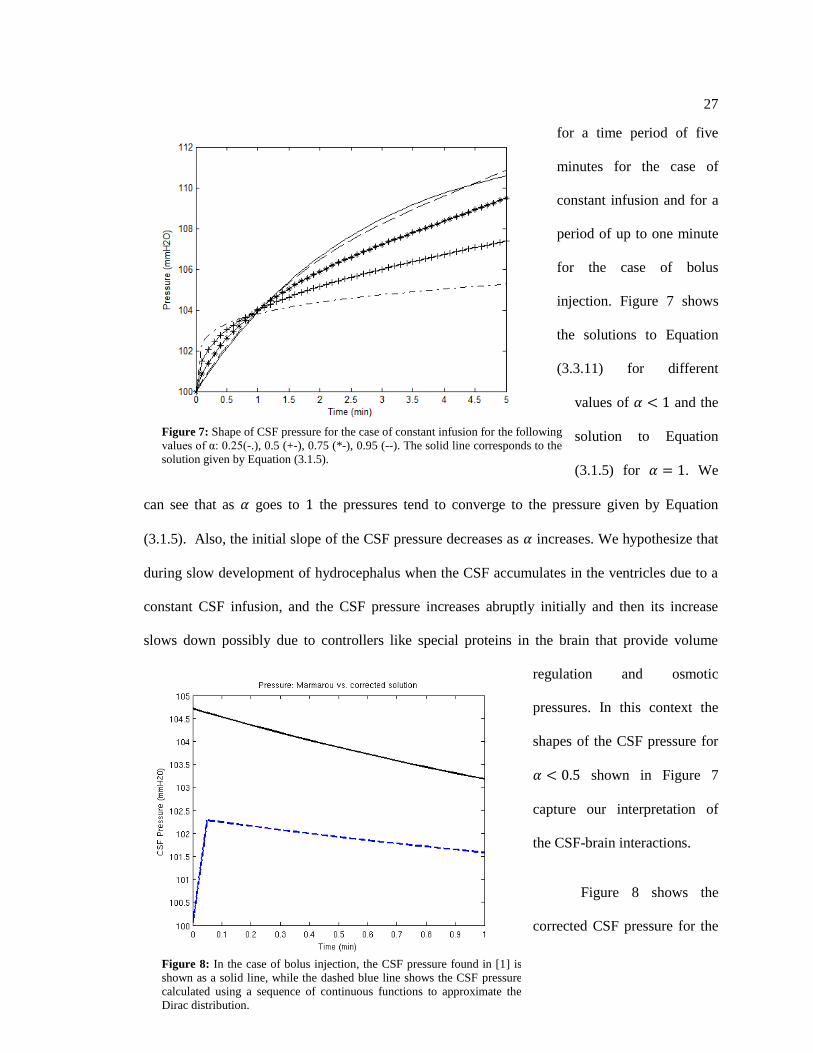
Figure 7: Shape of CSF pressure for the case of constant infusion for the following values

of α: 0.25(-.), 0.5 (+-), 0.75 (*-), 0.95 (--). The solid line corresponds to the solution

given by Equation (3.1.5). ................................................................................................ 27

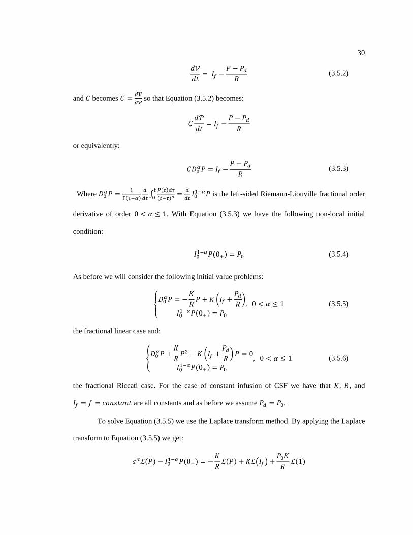
Figure 8: In the case of bolus injection, the CSF pressure found in [1] is shown as a solid

line, while the dashed blue line shows the CSF pressure calculated using a sequence

of continuous functions to approximate the Dirac distribution. ....................................... 27

Figure 9: The shapes of the CSF pressure for the case of bolus injection for the following

values of α: a) 0.05 (-.), 0.15(+-), 0.25 (*-), 0.35 (--). The solid line shows our

approximate solutions to Marmarou's model in this case. The largest radius of

convergence corresponds to and is given by , and b) 0.25 (-.),

0.5 (+-), 0.75 (*-), 0.95 (--). The solid line shows our approximate solutions to

Marmarou’s model in this case. The larges radius of convergence corresponds to

and is given by . .......................................................................... 29

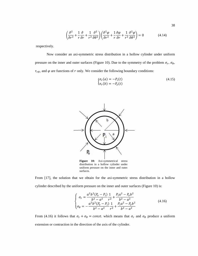
Figure 10: Axi-symmetrical stress distribution in a hollow cylinder under uniform

pressure on the inner and outer surfaces. ......................................................................... 38

Figure 11: Fractional linear case for bolus injection for values of: 0.25 (-.), 0.5 (+-),

0.75 (*-), 0.95 (--), 1 (solid). The solid line represents the classical solution. ................. 42

Figure 12: Fractional nonlinear case for bolus injection for α values of: 0.25 (-.), 0.5 (+-),

0.75 (*-), 0.95 (--), 1 (solid). The solid line represents the classical solution. ................. 43

Figure 13: Jacobian for (a) normal (red) and (b) hydrocephalic (blue) mice and their

corresponding polynomial fits.......................................................................................... 50

Figure 14: Healing (red) and inflammation (blue) state functions versus time for the

following initial conditions: a) – b) ; c) – d)

; e) – f) . The first column

represents the normal mice data, white the second column shows the hydrocephalic

mice data. In Matlab . .................................................................. 51

vi

LIST OF TABLES

Table 1: Analytic Solutions to equation (2.2.1) for the three different cases presented in

[1]. Note that is Pt the threshold pressure. ....................................................................... 8

Table 2: Calculated Jacobians from brain volumetric data for normal and hydrocephalic

mice. ................................................................................................................................. 49

vii

ACKNOWLEDGEMENTS

I would like to thank Dr. Corina Drapaca for all the support and help she has given me

the past two years. None of this would have been possible without that support. I would also like

to thank my committee members, Dr. Francesco Costanzo and Dr. Albert Segall, for their

comments and suggestions that helped improve my thesis.

I would also like to thank my parents, Chuck and Diane Kauffman, and my girlfriend,

Danielle Smith, who have always helped motivate me and never let me get discouraged.

I would finally like thank the Engineering Science and Mechanics department for

allowing me to continue my education and allowing me to meet me goals.

1

Chapter 1

Introduction

Hydrocephalus is a serious neurological disease that develops from abnormalities in the

circulation of cerebrospinal fluid (CSF). It results in ventricular dilation, compression of the brain

and a possible increase in intracranial pressure (ICP). Although hydrocephalus is one of the most

common neurological disorders treated by neurosurgeons, the cause of hydrocephalus is still

unknown because it can develop in conjunction with other neurological disorders, or even

infections resulting in inflammation of the brain.

The treatment of hydrocephalus is primarily based on diverting the CSF flow such that

the symptoms of the disease are reduced. This can be accomplished surgically by either

implanting a shunt into the ventricles or a procedure called endoscopic third ventriculostomy

(ETV). An implanted shunt redirects some of the excess CSF through a tube to the patient’s

stomach causing a decrease in the volume of the ventricles. However, shunt implantation has a

high risk of infection. On the other hand, ETV drains the ventricles through a hole made in the

third ventricle. In time this hole closes and a new surgery is often required. Clinical studies have

shown that neither of these treatments is effectively treating hydrocephalus. Shunts tend to be a

lifelong implant and tend to fail frequently among patients, while ETV is usually done only in

patients with a minimal risk in ventricular dilation in the future. Knowledge of the mechanics of

brain-ventricular CSF interface and the CSF circulation can help neurosurgeons determine which

treatment would result in a better outcome for a specific patient.

In order to improve the outcome of treatment and design new and better therapies for

hydrocephalus, we could benefit tremendously from accurate mathematical models describing the

2

CSF dynamics and CSF-brain interactions. Such models could help us understand the

fundamental science behind hydrocephalus. Marmarou et. al., [1] and Hakim et. al., [2]

developed the first models describing hydrocephalus. Marmarou modeled the CSF dynamics and

used experiments in cats to validate his model; whereas Hakim looked at the brain as a

viscoelastic material and proposed an engineering approach to explain the onset and evolution of

hydrocephalus using a series of controlled experiments. In this thesis we will develop a multi-

scale pressure-volume model describing the CSF dynamics. We will generalize Marmarou’s

model by using fractional calculus, and by doing this, we understand that we are changing the

physical meaning behind the original model. By using a fractional order temporal derivative we

introduce an inhomogeneous clock that connects continuously the global (macroscopic) time

scale to the local (microscopic) time scale. We solve our fractional differential equation

analytically using a modified Adomian decomposition method described in Duan et. al., [3]. We

compare our results to Marmarou’s classical solution and then use numerical simulations to show

the changes in displacement of the brain-ventricular CSF interface.

This thesis is structured as follows. Chapter 2 will be a brief review of Marmarou’s and

Hakim’s models followed by an introduction of fractional calculus and its application to neuronal

activity, and a description of the Adomian decomposition method used to analytically solve our

differential equations. In chapter 3 we will describe the classical Marmarou model, introduce our

fractional Marmarou model and compare the two models. We assume a cylindrical geometry of

the brain parenchyma and show the displacement fields of the brain-ventricular CSF interface

corresponding to the classic and fractional Marmarou models in Chapter 4. For the sake of

completeness, a presentation of the classic stress-strain analysis in a cylindrical domain is also

given in Chapter 4. Finally, in Chapter 5 we propose a totally different approach to studying

hydrocephalus. We introduce two states of the brain, healing (growth) and inflammation (aging),

and then invoke Hamilton’s principle, and investigate the interplay between these two states using

3

experimentally found brain volumetric data for healthy and hydrocephalic mice. Our preliminary

results show that inflammation overpowers healing in the case of untreated hydrocephalic mice,

while in the case of healthy aging mice, inflammation grows slowly with age and the healing

decreases as one would expect. The thesis ends with a chapter on conclusions and future work.

Our fractional Marmaou model will be published in [4, 5], while some of our work on the

coupled-field model of brain biomechanics using Hamilton’s principle will appear in [6].

4

Chapter 2

Literature Review

2.1 Hakim Model

Hakim et. al., [2] provided the first engineering approach to studying

hydrocephalus1. They had proposed a mathematical framework to study brain biomechanics along

with simplistic engineering systems while using experiments from a purely mechanics point of

view that explained the onset of hydrocephalus. The research that is presented in [2] is based on

several years of medical evidence on CSF dynamics. CSF is produced by the choroid plexus

which is located at the interface between the brain parenchyma and ventricles. Under normal

conditions CSF is produced at a constant rate and decreases as we get older. Despite the fact that

this knowledge is essential for hydrocephalus, we do not know the rate of CSF production and

there are no realistic or robust methods or technologies to measure or estimate it [8].

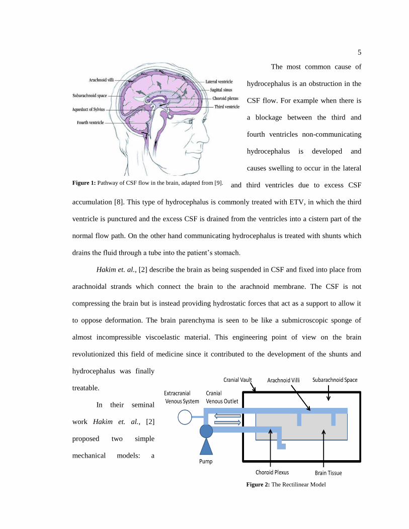
Figure 1 shows the pathway of CSF flow through the brain. The flow of the CSF

starts in the lateral and third ventricles and passes through the aqueduct of Sylvius to reach the

fourth ventricle. Once the CSF gets through the fourth ventricle it circulates into the subarachnoid

space [8]. A portion of the CSF flows down into the lumbar subarachnoid space; which, is

believed to be the cause of pulsations [10]. The CSF is then absorbed by the arachnoid villi

situated around the sagittal sinus [8]. It is not possible to undo absorption because the ICP is

greater than the sagittal sinus pressure ( ). Another possibility for CSF drainage is that some of

the CSF can “soak” through into the parenchyma [11].

1 This section is adapted from [7]

5

The most common cause of

hydrocephalus is an obstruction in the

CSF flow. For example when there is

a blockage between the third and

fourth ventricles non-communicating

hydrocephalus is developed and

causes swelling to occur in the lateral

and third ventricles due to excess CSF

accumulation [8]. This type of hydrocephalus is commonly treated with ETV, in which the third

ventricle is punctured and the excess CSF is drained from the ventricles into a cistern part of the

normal flow path. On the other hand communicating hydrocephalus is treated with shunts which

drains the fluid through a tube into the patient’s stomach.

Hakim et. al., [2] describe the brain as being suspended in CSF and fixed into place from

arachnoidal strands which connect the brain to the arachnoid membrane. The CSF is not

compressing the brain but is instead providing hydrostatic forces that act as a support to allow it

to oppose deformation. The brain parenchyma is seen to be like a submicroscopic sponge of

almost incompressible viscoelastic material. This engineering point of view on the brain

revolutionized this field of medicine since it contributed to the development of the shunts and

hydrocephalus was finally

treatable.

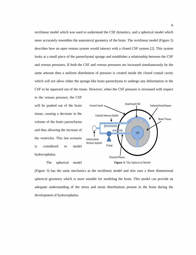
In their seminal

work Hakim et. al., [2]

proposed two simple

mechanical models: a

Figure 2: The Rectilinear Model

Figure 1: Pathway of CSF flow in the brain, adapted from [9].

6

rectilinear model which was used to understand the CSF dynamics, and a spherical model which

more accurately resembles the anatomical geometry of the brain. The rectilinear model (Figure 2)

describes how an open venous system would interact with a closed CSF system [2]. This system

looks at a small piece of the parenchymal sponge and establishes a relationship between the CSF

and venous pressures. If both the CSF and venous pressures are increased simultaneously by the

same amount then a uniform distribution of pressure is created inside the closed cranial cavity

which will not allow either the sponge-like brain parenchyma to undergo any deformation or the

CSF to be squeezed out of the tissue. However, when the CSF pressure is increased with respect

to the venous pressure, the CSF

will be pushed out of the brain

tissue, causing a decrease in the

volume of the brain parenchyma

and thus allowing the increase of

the ventricles. This last scenario

is considered to model

hydrocephalus.

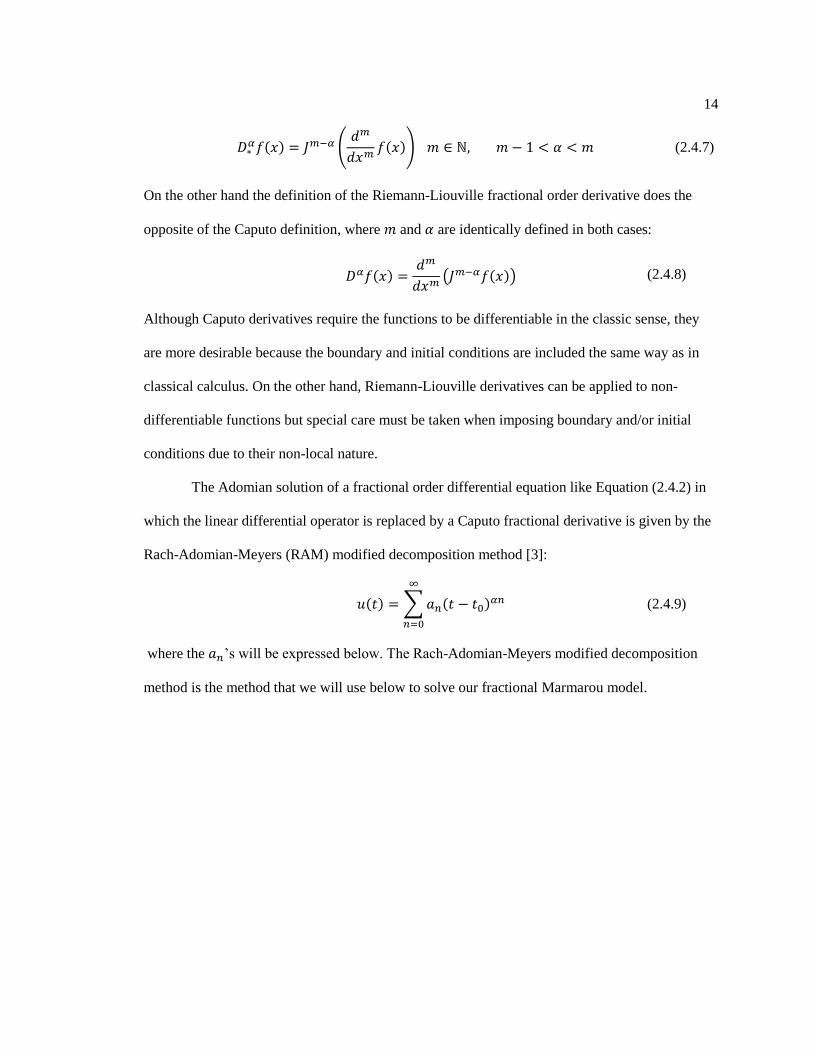
The spherical model

(Figure 3) has the same mechanics as the rectilinear model and also uses a three dimensional

spherical geometry which is more suitable for modeling the brain. This model can provide an

adequate understanding of the stress and strain distributions present in the brain during the

development of hydrocephalus.

Figure 3: The Spherical Model

7

2.2 Marmarou Model

Marmarou et. al., [1] developed the first mathematical model for CSF dynamics that

provided some essential insights into the role of ICP in hydrocephalus2. In order to avoid some

controversies with some terminology used in [1] that have been pointed out in the literature in

recent years, there will be no discussion here of some of the physical interpretations of

Marmarou’s model. The parameters that this model uses are dural sinus pressure, the resistance to

CSF absorption and the CSF formation rate. It is important to mention that Marmarou’s model

has been tested on adult cats and a good agreement has been established between the proposed

mathematical model and the measurements [1].

They noticed experimentally that as the fluid was either added or removed from the CSF

space, the pressure changed transiently and was followed by a gradual decline back to the initial

pressure. This occurs because the CSF volume and pressure are coupled. The rate of CSF

formation ( ) is composed of stored fluid ( ) and absorbed fluid ( ); under normal conditions

the formation of fluid and the absorption of fluid balance each other so that there is no change in

the amount of fluid stored. From this relationship Marmarou et. al., [1] developed a mathematical

model for the pressure ( ) at time ( ) represented by a nonlinear Riccati differential equation of

the form:

(

) (2.2.1)

where is a constant that describes the slope of the pressure-volume curve, is the resistance to

fluid flow, and is the intradural sinus pressure. For an initial condition ( ) , equation

(2.2.1) has a solution of the form:

2 This section is adapted from [7]

8

( )

( )

∫ ( )

( ) ∫ ( )

(2.2.2)

Marmarou et. al., [1] investigated three cases that can cause a change in the CSF volume:

1) bolus injection, 2) volume removal, and 3) continuous infusion. For each case ( ) is different

and thus different results for ( ) are obtained. The analytic solutions and ( ) for each case are

presented in Table 1. The derivations of these equations are given in [7].

Table 1: Analytic Solutions to equation (2.2.1) for the three different cases presented in [1]. Note that is Pt the

threshold pressure.

Case ( ) Analytic Solution

Bolus Injection ( ) ( ) ( )

( ⁄ )

[ ( ⁄ ) ]

Volume Removal ( ) ( )

{

( ) [ ] ( )

( )

( ⁄ )

[ ( ⁄ ) ]

Continuous Infusion ( ) ( )

( )

( ) ⁄

Figures 4-6 are plots of the analytic solutions to equation (2.2.2) corresponding to the

three cases. In the bolus injection case (Figure 4) some fluid is inserted into the CSF system

which adds to the formation rate of CSF. The system was in equilibrium before the fluid was

added and was at an initial pressure . The continuous infusion case (Figure 5) is very similar to

the bolus injection case but here the ICP increases rapidly and then stabilizes.

9

Figure 5: Analytic solution of Equation (2.2.2) for the continuous infusion case.

In the case of volume removal (Figure 6) an additional nonlinearity is introduced when

the ICP drops below the given threshold pressure which causes the resistance to absorption to be

Figure 4: Analytic Solution of Equation (2.2.2) for the bolus injection case.

10

increased and leads to a lack of absorption until the pressure meets the threshold pressure again

[1]. Once that happens absorption again takes place and the system will return to equilibrium.

Figure 6: Analytic Solution of Equation (2.2.2) for the case of volume removal.

2.3 Fractional Calculus

Below we will provide some background into the merit in using fractional calculus while

modeling the brain. Two models will be described. The first model uses fractional calculus to

model neuronal activity whereas the second describes the Hodgkin-Huxley model in terms of

fractional derivatives.

2.3.1 Fractional Model for Pyramidal Neurons

In [12] Lundstorm et. al. used fractional calculus to described the firing rate of pyramidal

neurons. It was originally thought that neurons followed a single time scale, but upon further

investigation Lundstorm et. al., [12] showed that the firing rate of neurons actually depends on

the history of the stimulus on that neuron. This implies that multiple time scales are needed to

11

describe the behavior of neurons, and this can be done using fractional differentiation. It should

be noted that fractional differentiation is non-local, so fractional order differentiation is indeed

using the history of neuronal activity to calculate the firing rate of the neuron. Lundstorm et. al.,

[12] discovered that there were a few different mechanisms that could have contributed to the

fractional order dynamics that they described. Different geometries of the cells or dendrites,

circuit and synaptic mechanisms, and many inactivation states of sodium channels could all

contribute to these fractional order dynamics. The use fractional differentiation enhances the

responses measured based off of changes in stimulus so that the magnitude and rate of change of

the signal is maintained. In addition, it seems that fractional order integration describes the

dynamics of muscles and tissue as well as their viscoelastic properties. Tying both fractional

order differentiation and integration together leads to multiple time scales that relate

deformations to different biological processes.

2.3.2 Generalization of Hodgkin-Huxley Model

The Hodgkin-Huxley model uses observations of axons from a giant squid to describe

mathematically how action potentials in neurons are initiated and propagated. The model is a

system of first order nonlinear ordinary differential equations for sodium activation, potassium

activation and leakage. In [13], Sherief et. al. generalized the model by replacing the first order

temporal derivatives with Caputo fractional order derivatives, described in more detail below.

They used the method of Laplace transforms and Mittage-Leffler functions (defined below) to

solve their fractional order differential equations. As the fractional order parameters approach

unity the solution of those parameters of the generalized model converges to the solution of the

classic Hodgkin-Huxley as one would expect.

12

2.4 Adomian Method

The Adomian method is a very powerful method for solving differential equations. The

method builds a series solution analytically to either an ordinary or partial differential equation

[14]. The Adomian series tend to converge quickly to the exact solution and therefore the number

of terms needed to obtain good approximations is small. It was shown that for simple geometries

the Adomian method performs better than classic numerical methods such as finite difference and

finite element methods. Recently the method has been extended to solve fractional differential

equations. Below we will describe the original Adomian method and then show one of its

adaptations for fractional order differential equations which we will use in this thesis.

2.4.1 Classical Adomian Method

The Adomian method takes a differential equation, either partial or ordinary and

separates it into a linear part and nonlinear part [14]. The linear part can further be decomposed

into an easily invertible part and a remainder. So the differential equation looks like:

(2.4.2)

where is the easily invertible term, is the remainder of the linear term that is not easily

invertible, and is the nonlinear term as defined by [14]. Once we have our differential equation

in this form we want to solve for . Since is easily invertible, we can take of both sides of

Equation (2.4.2). Note that ( ) ( ) . We look for a solution of

the form:

∑

(2.4.3)

which replaced into Equation (2.4.2) gives:

13

∑

∑

∑

(2.4.4)

where , and it is assumed that the nonlinear term was an analytic function of

that can be written as a series expansion of the so-called Adomian polynomials

∑ ( ) ( )( ) where is of increasing index, is the order of the polynomial, and the

sum of the subscripts must add to since is defined in terms of , , , .

The Adomian method has the advantage that we do not have to apply simplifying

assumptions where we linearize our equation or subject it to perturbations [14]. A fast converging

series solution is more desirable than changing the original problem and having a closed form

solution which might be far off from the solution to the original problem.

2.4.2 Fractional Adomian Decomposition Method

Even though fractional order derivatives and integrals have been around since the 17th

century, the physical and geometrical interpretations of these fractional order derivatives and

integrals has, only recently, been provided by [15] and because of this fractional calculus is now

being used for some applications. The most common fractional order derivatives are Riemann-

Liouville and Caputo. The Riemann-Liouville integral of order is defined as:

( )

( )∫ ( )

( ) (2.4.5)

and it should be noted that [3]:

( ) ∫

( )

( ) ( )

∫

( ) ( )

(2.4.6)

The definition of the Caputo fractional order derivative tells us to first take ordinary derivatives

then a fractional integral:

14

( ) (

( )) (2.4.7)

On the other hand the definition of the Riemann-Liouville fractional order derivative does the

opposite of the Caputo definition, where and are identically defined in both cases:

( )

( ( )) (2.4.8)

Although Caputo derivatives require the functions to be differentiable in the classic sense, they

are more desirable because the boundary and initial conditions are included the same way as in

classical calculus. On the other hand, Riemann-Liouville derivatives can be applied to non-

differentiable functions but special care must be taken when imposing boundary and/or initial

conditions due to their non-local nature.

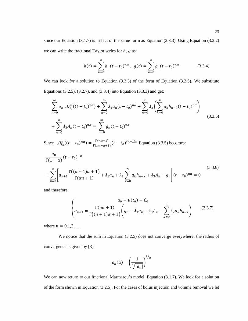
The Adomian solution of a fractional order differential equation like Equation (2.4.2) in

which the linear differential operator is replaced by a Caputo fractional derivative is given by the

Rach-Adomian-Meyers (RAM) modified decomposition method [3]:

( ) ∑ ( )

(2.4.9)

where the ’s will be expressed below. The Rach-Adomian-Meyers modified decomposition

method is the method that we will use below to solve our fractional Marmarou model.

15

Chapter 3

Fractional Marmarou Model

In this chapter we will develop and solve a fractional Riccati differential equation using

the Laplace transform method and the Rach-Adomian-Meyers (RAM) decomposition method.

First, we will present the classical equation developed by [1] followed by a presentation of the

linear fractional case and then the fractional Riccati equation.

3.1 Classic Marmarou Model

For the sake of completeness we present again Marmarou’s model. Marmarou’s model

[1] is based on the conservation law where the rate for formation of the CSF, , is known and is

equal to the sum of the rate of volume change of the CSF stored in the ventricles of the brain,

, where is the volume of CSF, and the rate of outflow (absorption) of the CSF,

, where is the resistance of CSF absorption, is the pressure of the CSF, and is the

pressure of the venous system:

(3.1.1)

or

(3.1.2)

Marmarou introduced the so-called compliance of the CSF system

, used the chain

rule,

and transformed Equation (3.1.2) into:

(3.1.3)

16

which is a first order differential equation that is linear in the unknown ( ) if ( ),

and ( ). Now if we assume that

where is a parameter of Marmarou’s model,

then Equation (3.1.3) becomes a Riccati differential equation of the form:

(

) (3.1.4)

When the initial condition is ( ) , the solution to Equation (3.1.2) is:

( ) ∫ ( )

∫ ∫ ( )

(3.1.5)

where we denote ( ) ( )

.

The brain has special properties that provide volume regulation and osmotic pressure that

controls CSF flow. In addition, the measurements of CSF pressure are prone to errors due to the

complex dynamics of the brain. In order to account not only for the biomechanical behavior of

the brain which is still barely known, but also for the uncertainties in CSF pressure measurements

in the simplest possible way, we propose to use the fractional Caputo derivative, denoted as

,

of order instead of the first order derivative in Equation (3.1.4). It should be noted

that the notation between the Caputo order fractional derivative and the Riemann-Liouville

fractional derivative is differentiated by the . Therefore, we propose the following

generalizations to Equations (3.1.3) and (3.1.4):

{

( )

( )

(3.1.6)

and respectively if

:

{

(

)

( ) (3.1.7)

Again, in Equations (3.1.6) and (3.1.7) we denote

by:

17

( )∫

( )

( )

(3.1.8)

the Caputo derivative of order . Our fractional models, Equations (3.1.6) and (3.1.7),

are based on the assumption that the conservation law of CSF hydrodynamics used in the

Marmarou model remains valid when the first order time derivative is replaced by a fractional

order derivative. We also notice that although we continue to use the same notations and

definitions for the physical quantities and parameters in our models, as in Marmarou’s model,

they have now different physical units and physical meanings. In our future work we plan to

study the physical interpretation of these quantities. Lastly, we point out that our models capture a

temporal multiscale effect if we allow to vary.

We will solve Equation (3.1.6) for

to gain some insight into the

behavior of and then we will solve Equation (3.1.7). Equation (3.1.6) is the fractional

linear equation where the solution will be presented in the next section. Equation (3.1.7) is the

fractional Riccati differential equation and will be solved in the third section of this chapter.

First we should note that the solution to (3.1.6) when is the classic solution to a

first order linear differential equation:

{

(

)

( )

(3.1.9)

where the solution takes the form:

( ) ( ( ) )

⁄ (3.1.10)

Note that here

, and has different physical units than in [1] where

. For simplicity

we will consider throughout this thesis.

18

3.2 Fractional Linear Marmarou Model

Here we present two methods to solve Equation (3.1.6): the Laplace transform method,

and the RAM decomposition method (which we will use to solve Equation (3.1.7) as well).

Before we do this we should again state that we are aware that the physical meaning of the law in

question has been changed, but we will use this model to gain some insight into the behavior of

the fractional model proposed. Now let us first consider the Laplace transform method we denote

the Laplace transform of by ( )( ) ∫

( ) . It can be shown that (

)

( ) ( ). So, by taking the Laplace transform of Equation (3.1.6), we obtain:

( ) ( )

( ) (3.2.1)

Where the term

corresponds to ( ). We recall that ( ) ( ) ( ) where

∫ ( ) ( )

is the convolution operation.

We can simplify Equation (3.2.1) to get:

( )

( )

⁄

(3.2.2)

Also, from the properties of the Mittag-Leffler function [3, 15], and the generalized Mittag-

Leffler function we know that:

{

( ) ∑

( )

( ) ∑

( )

{

( ( ))

( ( ) ( ))

respectively. Therefore from the above formulas we obtain:

19

( ) (

) ∫ ( ) (

) ( )

∫ ( ) (

)

(3.2.3)

Now we develop the solution from the RAM modified decomposition method proposed by Duan

et. al., [3]. The method says that the solution to:

{

( ) ( ) ( ( )) ( )

( )

( ) ( ) ( )( )

(3.2.4)

where , is:

( ) ∑ ( )

(3.2.5)

where

{

( )

( )( )

(3.2.6)

with

{

( ) ∑ ( )

( ( )) ∑ ( )

( )

(3.2.7)

and the ’s are the corresponding Adomian polynomials defined as [3, 14, 15]:

{

( )

( )

( )

( )

(3.2.8)

For simplicity we will consider the case of constant infusion of CSF.

20

( ) {

(3.2.9)

In this case our solution Equation (3.2.3) becomes:

( ) (

) ∫ (

) ( ) (

)

(3.2.10)

based on the Laplace transform method, while the RAM decomposition method give the

following solution:

( ) ∑

(3.2.11)

where

( )( (

)

)

( )

( )(

)

( )

( )(

)

(3.2.12)

Plugging in the coefficients in Equation (3.2.12) into Equation (3.2.11) and comparing the results

to Equation (3.2.10) it can be shown the solutions do agree as they should. Therefore, both the

Laplace transform method and the RAM modified decomposition method give the same results.

This validates the RAM decomposition method which we will use further to solve Equation

(3.1.7).

21

3.3 Fractional Nonlinear Marmarou Model

In this section we will develop solutions to Equation (3.1.7). For this differential equation

we will consider the three different cases that are presented in [1]: bolus injection, volume

removal, and continuous infusion. Bolus injection and volume removal differ only by a sign so

they will be solved together using the operator to distinguish between the two. Note that bolus

injection corresponds to the plus and volume removal corresponds to the minus. We will start by

first considering bolus injection/volume removal and then move on to continuous infusion at the

end of this section.

3.3.1 Bolus Injection/Volume Removal

For the case of bolus injection/volume removal ( ). Since the case of

constant infusion (discussed below) accounts for the constant term in we can restrict the cases

of bolus injection/volume removal to just the term described by the Dirac delta function because a

linear superposition of the solutions in the constant infusion case and either in the bolus injection

or in the volume removal case will get us back to the original definition described in [1]. So

without loss of generality we will consider the case when ( ) ( ). For these two cases

the solutions proposed by Marmarou are not valid. As we have mentioned in Chapter 2,

Marmarou et. al., [1] used the integration factor method to solve Equation (3.1.4), but this

method does not work under the case when ( ) because the Dirac delta function is not

continuous. Also, it should be noted that at short time scales Marmarou’s solutions for these two

cases do not satisfy the initial conditions proposed by Marmarou et. al., [1]. To develop a valid

solution we must use a continuous approximation of the Dirac delta function. We choose

( )

| | , where the function ( )

| | is continuous , . Thus

22

for the cases of bolus injection and volume removal we can solve Equation (3.1.4) for

( ) using the integrating factor method and so we get from Equation (3.1.5):

( )

∫ (

⁄ )

∫

∫ (

⁄ )

or equivalently:

( )

(

)

∫

(

)

(3.3.1)

The integral in Equation (3.3.1) are evaluated numerically. Then the solution is:

( )

( )

To solve Equation (3.1.7) we will again use the RAM decomposition method outlined in

[3] and Equation (3.2.4) – (3.2.8), and the fractional Taylor series representation of a function

expressed with the help of the Caputo fractional derivatives of order [16]:

( ) ∑

( )

( )

( )

(3.3.2)

where

, where

on the left side, and on the

right side are repeated times. We can use Equation (3.3.2) to find the needed coefficients in

Equation (3.2.7).

We propose now a small generalization to the theory presented in [3], namely we want to

use the RAM modified decomposition method to solve the following variation to Equation

(3.2.4):

{

( ) ( ) ( ) ( ) ( ( )) ( )

( )

(3.3.3)

23

since our Equation (3.1.7) is in fact of the same form as Equation (3.3.3). Using Equation (3.3.2)

we can write the fractional Taylor series for , as:

( ) ∑ ( )

( ) ∑ ( )

(3.3.4)

We can look for a solution to Equation (3.3.3) of the form of Equation (3.2.5). We substitute

Equations (3.2.5), (3.2.7), and (3.3.4) into Equation (3.3.3) and get:

∑

(( ) )

∑ ( )

∑ (∑ ( )

)

∑ ( )

∑ ( )

(3.3.5)

Since (( )

) ( )

( )( )

( ) Equation (3.3.5) becomes:

( )( )

∑ [

(( ) )

( ) ∑

] ( )

(3.3.6)

and therefore:

{

( )

( )

(( ) )( ∑

) (3.3.7)

where .

We notice that the sum in Equation (3.2.5) does not converge everywhere; the radius of

convergence is given by [3]:

( ) (

√| | )

⁄

We can now return to our fractional Marmarou’s model, Equation (3.1.7). We look for a solution

of the form shown in Equation (3.2.5). For the cases of bolus injection and volume removal we let

24

( ) ( ), take ( )

√

( )⁄ (this choice makes the calculations

simpler) and solve:

{

(

√

( )⁄

)

( )

(3.3.8)

Thus for the cases of bolus injection and volume removal ( ) ( ) where is the

solution to Equation (3.3.8).

Since Equation (3.1.7) is of the form of Equation (3.3.3) we get from the formulas

presented above that:

( ) ∑

with

{

( )

( )(

∑

)

{

where the Adomian polynomials correspond to ( ) . We also have that:

( ) ∑

( )

( )

√

( )⁄

with

( )

( )

∫

( )

( )

25

We denote by

( )

( ) and these are some of the parameters needed to calculate above.

Therefore:

(3.3.9)

with

( )

( )(

( ) )

(3.3.10)

has this form since and in we have that:

( ) ( )

√ ∫

( )⁄

( )

3.3.2 Continuous Infusion

In this case we use directly the RAM decomposition method to solve Equation (3.1.7).

We denote by:

{ (

)

(3.3.11)

and rewrite Equation (3.1.7) as:

{

( )

(3.3.12)

whose solution is according to Equation (3.2.5) of the form:

26

( ) ∑

(3.3.13)

where

( )

( )( )

with Adomian polynomials:

∑

3.4 Results

For our numerical simulations we used the following parameters that were found

experimentally by [1] while they were investigating possible mechanisms for the onset of

hydrocephalus in adult cats: [ ], ⁄ [ ],

[ ], [ ], a constant rate of infusion [ ] in the

constant infusion case, and [ ] in bolus injection. Note that we are not showing any

results from the case of volume removal since it is similar to the the case of bolus injection.

Given that the duration of the experiments in [1] were on the order of six to eight minutes, and

that the radii of convergence of our series solutions impose limitations we will show our results

27

for a time period of five

minutes for the case of

constant infusion and for a

period of up to one minute

for the case of bolus

injection. Figure 7 shows

the solutions to Equation

(3.3.11) for different

values of and the

solution to Equation

(3.1.5) for . We

can see that as goes to the pressures tend to converge to the pressure given by Equation

(3.1.5). Also, the initial slope of the CSF pressure decreases as increases. We hypothesize that

during slow development of hydrocephalus when the CSF accumulates in the ventricles due to a

constant CSF infusion, and the CSF pressure increases abruptly initially and then its increase

slows down possibly due to controllers like special proteins in the brain that provide volume

regulation and osmotic

pressures. In this context the

shapes of the CSF pressure for

shown in Figure 7

capture our interpretation of

the CSF-brain interactions.

Figure 8 shows the

corrected CSF pressure for the

Figure 7: Shape of CSF pressure for the case of constant infusion for the following

values of α: 0.25(-.), 0.5 (+-), 0.75 (*-), 0.95 (--). The solid line corresponds to the

solution given by Equation (3.1.5).

Figure 8: In the case of bolus injection, the CSF pressure found in [1] is

shown as a solid line, while the dashed blue line shows the CSF pressure

calculated using a sequence of continuous functions to approximate the

Dirac distribution.

28

case of bolus injection (dashed blue line) using an approximation for the Dirac distribution which

is then compared to the original solution proposed by [1]. The two solutions do not agree on short

times, which was expected, although at longer times the two solutions will eventually coincide. In

Figure 9a and 9b we show the temporal variations of the CSF pressure as given by Equations

(3.3.9) and (3.3.10). While the initial slope of the pressure decreases as approaches , the

pressure given by Equations (3.3.9) and (3.3.10) does not converge to the CSF pressure calculated

using an approximation of the Dirac distribution (Figure 9b).

In our future work we plan to add more terms to Equation (3.3.9) as well as use Padé

Approximates as in [3] to get the expected convergence as goes to . We will also implement

better numerical solvers for the coefficients of of the fractional Taylor series of

( ) needed in Equation (3.3.10). We should note that if after all of these improvements we still

see the same asymptotic behavior of the CSF pressure for (Figure 9a) we could

hypothesize that at later times the CSF volume may increase and then it could model the slow

development of hydrocephalus. This means that bolus injection of CSF could in fact cause

hydrocephalus when the CSF-brain dynamics has been somehow compromised3. Thus, our

fractional pressure-volume model appears to capture certain processes happening at time scales of

order which could cause the onset of hydrocephalus either by constant infusion of CSF

or by CSF bolus injection. A constant infusion CSF is by now a known and accepted mechanism

for hydrocephalus; however, the bolus injection is a new and rather unexpected cause of

hydrocephalus. A deeper and more thorough analysis of our model along with experiments is

needed in order to consider this as plausible.

3 We suspect that in hydrocephalus the CSF is a non-Newtonian fluid (while in healthy subjects it

is already known that the CSF is Newtonian). Dr. Steven Schiff, Private communication.

29

3.5 Concluding Remarks

Before moving to the next chapter, we would like to mention another possible

generalization of Marmarou’s model using the left Riemann-Liouville fractional order derivative.

We start by defining some “averaged” values of the CSF volume and pressure as:

{

( )

( )

( )∫

( )

( )

( ) ( )

( )∫

( )

( )

(3.5.1)

These new quantities ( ) and ( ) are multiscaled volume and pressure in time because of the

fractional order integral, . Thus, from a practical point of view, these quantities should be

less sensitive to inherent measurement errors than ( ) and ( ).

Marmarou’s conservation law Equation (3.1.2) becomes in this case:

Figure 9: The shapes of the CSF pressure for the case of bolus injection for the following values of α: a) 0.05 (-.), 0.15(+-),

0.25 (*-), 0.35 (--). The solid line shows our approximate solutions to Marmarou's model in this case. The largest radius of

convergence corresponds to and is given by , and b) 0.25 (-.), 0.5 (+-), 0.75 (*-), 0.95 (--). The solid

line shows our approximate solutions to Marmarou’s model in this case. The larges radius of convergence corresponds to

and is given by .

30

(3.5.2)

and becomes

so that Equation (3.5.2) becomes:

or equivalently:

(3.5.3)

Where

( )

∫

( )

( )

is the left-sided Riemann-Liouville fractional order

derivative of order . With Equation (3.5.3) we have the following non-local initial

condition:

( ) (3.5.4)

As before we will consider the following initial value problems:

{

(

)

( )

(3.5.5)

the fractional linear case and:

{

(

)

( )

(3.5.6)

the fractional Riccati case. For the case of constant infusion of CSF we have that , , and

are all constants and as before we assume .

To solve Equation (3.5.5) we use the Laplace transform method. By applying the Laplace

transform to Equation (3.5.5) we get:

( )

( )

( ) ( )

( )

31

and since ( ) ⁄ , ( ) ( ), and

( ) the above equation simplifies to:

(

) ( ) (

)

Now recalling that ( ( ) ( ))

and (∫ ( )

)

( ) we get that the

solution to Equation (3.5.5) of the form:

( )

( ) (

) (

)∫ ( ) (

)

(3.5.7)

To solve Equation (3.5.6) we use the RAM decomposition method and look for a solution of the

form ∑ with

and ∑ , where ’s are the same Adomain

polynomials we used to solve the fractional Riccati differential equation with the Caputo

fractional derivative. Let

and ∫

be operators. We then have:

|

(

)

such that:

(

)

( )

which we can further written as:

(∑

) (

) (∑

)

( )

with

{

(

)

( (

))

(

)

( (

))

(

)

( (

))

Whereas before

32

It is known that the following inversion formula is true for the left-sided Riemann-

Liouville derivative and the Riemann-Liouville integral:

Thus if we want to solve for for the unknown we just need to:

Which gives:

( )

( )

and so

(

( ))

Next, we need to solve the following for :

| (

)∫

( )

∫ (

( ))

which evaluates to:

|

( )(

)

( )

33

Therefore:

( )(

)

( ) ( )

It is known that:

( )

( )

and therefore:

( )

( ) ( )

( )

( )

( )

( ) ( )

( )

( )

We finally get:

(

)

( )

( ) ( )

( )

( ) ( ) ( )

and

( ) [ (

)

( )

( ) ( )

( )

( ) ( ) ( ) ]

We follow the same procedure for and end up with:

(

) ( ) ( )

( ) ( ) ( )

( ) ( )

( )( ) ( ) ( ) ( )

(

)

( ) ( )

( ) ( ) ( ) ( )

( ) ( )

( ) ( ) ( ) ( )

And now can now be calculated. Therefore the solution to Equation (3.5.6) is:

(3.5.8)

In most cases the Adomian series converges to the solution of a given initial (or

boundary) value problem in four to six terms. We note that we could calculate more terms

through symbolic computations on a computer. Also, for Equation (3.5.8) should be the

34

Mclaurin series of the classic Riccati differential equation proposed by Marmarou et. al., [1]. In

our further work we intend to solve Equations (3.5.5) and (3.5.6) for the cases of bolus

injection/volume removal and compare the results obtained for the Riemann-Liouville fractional

and the Caputo fractional Riccati differential equations.

35

Chapter 4

Stress Strain Analysis in a Cylindrical Geometry with Applications to Brain-

CSF Interactions

In this chapter we investigate the effects of the behavior of CSF dynamics on brain tissue.

For simplicity we use a cylindrical geometry of the brain and the CSF dynamics is described by

either Marmarou’s model or by our (Caputo) fractional Marmarou model.

4.1 Theory

We present first a classic two-dimensional problem in elasto-statics4 [17]. We denote by

(

) (4.1)

a plane stress field acting on a body where weight is the only force. We assume that the density is

uniform in the body, . The equilibrium equations are in this case:

{

(4.2)

where we need to solve for , , and so that they will satisfy the boundary conditions.

System (4.2) is indeterminate because we have three unknowns, and only two equations. To get

this third equation we must use the condition of compatibility of strains so that we can guarantee

the existence of the displacement components, and . For infinitesimal deformations in plane,

the strain components are:

4 This chapter is adapted from [7]

36

(4.3)

It can be shown that the condition of integrability for (4.3) is:

(4.4)

which is also known as the condition of compatibility for admissible strains.

We further assume that the body is made of an isotropic linear elastic material, and

therefore the inverse form of Hooke’s Law is:

{

( )

( )

( )

(4.5)

with being Young’s modulus and Poisson’s ratio. By replacing (4.5) into (4.3) the expression

in the stresses of the condition of compatibility is:

( )

( ) ( )

(4.6)

By combining the two equations in (4.2) the system is reduced to:

(

) (4.7)

which replaced into (4.6) gives the following Laplace equation:

(

) ( ) (4.8)

and, therefore, (4.2) and (4.8) along with the corresponding boundary conditions can now be

solved for the unknown stresses , , and .

In 1862 Airy had introduced the so-called Airy stress function ( )such that:

37

{

(4.9)

which when replaced into (4.8) gives the Airy equation for :

(4.10)

The solution to (4.10) for will then give , , and from (4.9).

Now we will introduce polar coordinates:

{

{

(

⁄ ) {

(4.11)

where , , and , , are respectively orthonormal tangent systems in Cartesian and polar

coordinates, and {

which implies that

{

.

Thus system (4.2), in the absence of any body forces, in polar coordinates becomes:

{

(4.12)

While equations (4.9) and (4.10) become:

{

(

)

(4.13)

and

38

(

)(

) (4.14)

respectively.

Now consider an axi-symmetric stress distribution in a hollow cylinder under uniform

pressure on the inner and outer surfaces (Figure 10). Due to the symmetry of the problem , ,

, and are functions of only. We consider the following boundary conditions:

{ ( ) ( )

( ) ( )

(4.15)

From [17], the solution that we obtain for the axi-symmetric stress distribution in a hollow

cylinder described by the uniform pressure on the inner and outer surfaces (Figure 10) is:

{

( )

( )

(4.16)

From (4.16) it follows that which means that and produce a uniform

extension or contraction in the direction of the axis of the cylinder.

e

Figure 10: Axi-symmetrical stress

distribution in a hollow cylinder under

uniform pressure on the inner and outer

surfaces.

39

The radial displacement is found now from:

( ) (4.17)

since in the two-dimensional case, the strain tensor in polar coordinates is related to the

displacement field ( ) we get that the strain tensor in polar coordinates is:

{

(4.18)

We replace now equation (4.16) into the inverse form of Hooke’s Law in polar coordinates:

{

( )

( )

(4.19)

where

( ) is the modulus of rigidity (or elasticity in shear), use the fact that axi-

symmetrical cylinder requires , and get:

[( )

( ) ( ) ( ) ( ) ] (4.20)

Thus:

( )

[

( )

( ) ( ) ( ) ( ) ] ( ) (4.21)

and

( ) (4.22)

Integrating (4.22) we get:

40

( )

∫ ( ) ( ) (4.23)

Now by replacing both and into we get that:

( )

( )

∫ ( )

( ) (4.24)

This means that ( ) and ( ) . Therefore,

{

( )

[

( )

( ) ( ) ( ) ( ) ]

( )

(4.25)

with , , , , , and being constants.

However the term

in the expression of is multivalued, i.e. it changes by as the

coordinate goes around the circle once; this implies that , since the displacement field

must be single-valued.

By imposing the boundary conditions from equation (4.15), it can be shown that:

(

( )

( )

)

( )

( )

( )

(4.26)

But from equation (4.18):

(4.27)

and since the problem is axi-symmetric with all the involved functions being dependent only on

, it finally follows that:

( )

( )

( )

( )

(4.28)

The above calculations are intended to be used in the numerical simulations describing

brain biomechanics, with the application to hydrocephalus. Therefore, it is assumed that the brain

41

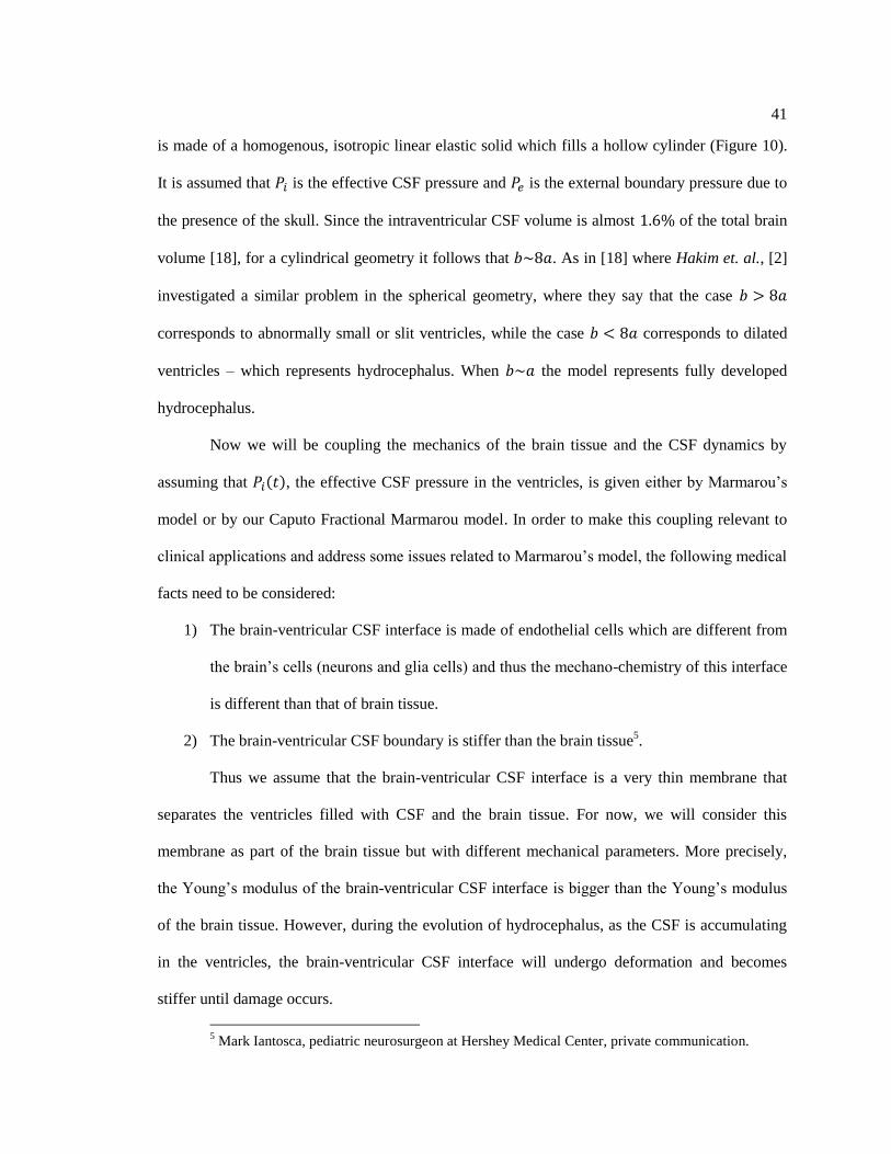
is made of a homogenous, isotropic linear elastic solid which fills a hollow cylinder (Figure 10).

It is assumed that is the effective CSF pressure and is the external boundary pressure due to

the presence of the skull. Since the intraventricular CSF volume is almost of the total brain

volume [18], for a cylindrical geometry it follows that . As in [18] where Hakim et. al., [2]

investigated a similar problem in the spherical geometry, where they say that the case

corresponds to abnormally small or slit ventricles, while the case corresponds to dilated

ventricles – which represents hydrocephalus. When the model represents fully developed

hydrocephalus.

Now we will be coupling the mechanics of the brain tissue and the CSF dynamics by

assuming that ( ), the effective CSF pressure in the ventricles, is given either by Marmarou’s

model or by our Caputo Fractional Marmarou model. In order to make this coupling relevant to

clinical applications and address some issues related to Marmarou’s model, the following medical

facts need to be considered:

1) The brain-ventricular CSF interface is made of endothelial cells which are different from

the brain’s cells (neurons and glia cells) and thus the mechano-chemistry of this interface

is different than that of brain tissue.

2) The brain-ventricular CSF boundary is stiffer than the brain tissue5.

Thus we assume that the brain-ventricular CSF interface is a very thin membrane that

separates the ventricles filled with CSF and the brain tissue. For now, we will consider this

membrane as part of the brain tissue but with different mechanical parameters. More precisely,

the Young’s modulus of the brain-ventricular CSF interface is bigger than the Young’s modulus

of the brain tissue. However, during the evolution of hydrocephalus, as the CSF is accumulating

in the ventricles, the brain-ventricular CSF interface will undergo deformation and becomes

stiffer until damage occurs.

5 Mark Iantosca, pediatric neurosurgeon at Hershey Medical Center, private communication.

42

4.2 Results

Here we will present plots showing how our fractional model has affected the

displacement. We expect that the displacements will follow the trends that were presented above

when we displayed the pressure versus time plots. We had found this to be true in [7], so the

fractional models should follow the same trend. Since our fractional model for the case of

continuous infusion approached the classical solution as converged the deformations will

follow the same trend that was found in [7]; therefore, the plots for this case are not presented

here because they do not lead to any further insight. Although, in the case of the bolus injection

we have shown that our fractional model does not approach the classical solution, so it is

interesting to see if the deformations follow the same behavior.

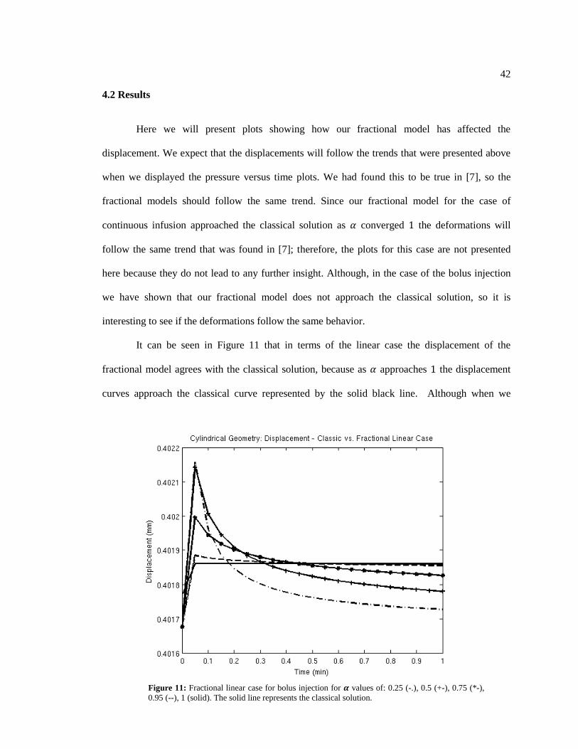
It can be seen in Figure 11 that in terms of the linear case the displacement of the

fractional model agrees with the classical solution, because as approaches the displacement

curves approach the classical curve represented by the solid black line. Although when we

Figure 11: Fractional linear case for bolus injection for values of: 0.25 (-.), 0.5 (+-), 0.75 (*-),

0.95 (--), 1 (solid). The solid line represents the classical solution.

43

consider our nonlinear fractional model it does not agree with the classical solution, but does

indeed agree with our findings from above. Since our fractional model did not agree in terms of

the pressure versus time the displacement curves also do not agree. Given that this was true for

the case of continuous infusion it makes sense that it would be the same for the case of bolus

injection. In Figure 12 we see the increase in displacement for values of less than , so it

appears that a bolus injection of CSF could contribute to the onset of hydrocephalus.

Figure 12: Fractional nonlinear case for bolus injection for α values of: 0.25 (-.), 0.5 (+-), 0.75 (*-),

0.95 (--), 1 (solid). The solid line represents the classical solution.

44

Chapter 5

Brain Biomechanics using Hamilton’s Principle

In this chapter we propose a coupled-field model and use Hamilton’s principle to

investigate the onset and evolution of hydrocephalus.

5.1 Theory

In this section we present a one-dimensional model for brain dynamics using Hamilton’s

principle. For simplicity, we assume that in the healthy state only small macro-deformations

(linear kinematics) can occur in the brain tissue and the mechanical response of the brain tissue at

the macroscopic level is linear visco-elastic of Kelvin-Voight type (the stress field in such a

material is the sum of a (linear viscous) stress component proportional to the strain rate). The

one-dimensional brain tissue of length has one fixed boundary ( ) at the interface with the

meninges surrounding the brain and one moving boundary ( ) at the interface with the

ventricular CSF which undergoes macroscopic displacements caused by the heart pulsations and

healthy aging.

We assume further that there are two biological processes happening on different time

scales that are important to the proper functionality of the brain: 1) a microstructural healing of

the brain and we denote this by ( ) the current healing state function, and 2) a

microstructural inflammation of the brain that progresses slowly throughout the entire life and we

denote this by ( ) the current inflammation state function. Our second assumption is based

on clinical studies [19] that have shown that inflammation plays an important role in the process

of normal aging and age-related diseases. In addition, we suggest inflammation of the brain, and,

45

more specifically, of the choroid plexus (anatomical structure located at the interface between the

brain tissue and the ventricular CSF which is involved in the CSF production) as one possible

mechanism for the onset of postinfectious and posthemorrhagic pediatric hydrocephalus.

We generalize the theoretical concepts introduced in [20] and adapt them to our model’s

assumptions. We propose a Lagrangian of the form:

∫ [

(

)

( )

(

)]

(5.1)

where is the mass density of the one dimensional brain tissue of length and constant cross-

sectional area , ( ) is the macroscopic displacement, is the effective macroscopic elastic

modulus, and , are positive constants for simplicity, but in general and will not be the

same for each term in the sum so they would not be able to be factored out was we have shown.

For simplicity, we denote ⁄ and

⁄ . The second and fourth terms of Equation

(5.1) represent microstructural kinetics and respectively energies caused by the evolution of the

brain’s microstructure due to normal healing and inflammation. Similar terms have been

proposed before in phase-field models of continua undergoing changes in phase [21,22] and in

damage mechanics [20]. As we learn more about the brain, we will improve our definitions and

concepts introduced in this model.

As in [20] we defined the virtual work done by non-conservative forces as:

∫ [ ( ) (

) ]

| (5.2)

where is a body force per unit length, is the linear damping term of the Kelvin-Voight

model with the viscosity and , are generalized forces that are work conjugates of the

evolution variables , . Also, is a concentrated load on the ventricular CSF-brain interface.

We employ now the non-conservative form of Hamilton’s principle:

46

∫ ( )

(5.3)

where the variations in the field variables , , are taken to be independent, vanish at the

arbitrary times , , and satisfy the kinematically admissible geometric boundary conditions.

By definition, the variation of the Lagrangian given by Equation (5.1) is:

( )|

∫ [ ( )

(

)

(

)]

(5.4)

We replace Equations (5.2) and (5.4) into Hamilton’s principle, Equation (5.3), use integration by

parts and the facts that the variations , , are independent, and vanish at the arbitrary

times , to obtain the following system of partial differential equations:

( ) (5.5)

(5.6)

(5.7)

We note that Equation (5.7) is in fact the conservation law of linear momentum for our problem

of a Kelvin-Voight material of strain and stress .

To the system created by Equations (5.5) to (5.7) we add boundary conditions:

( ) ( ) ( ) (5.8)

and Dirichlet and/or Neumann boundary conditions at for , .

47

We can show now that Equation (5.2) is consistent thermodynamically. If we ignore

thermic effects, then the total energy is the sum of all the mechanical energies given in Equation

(5.1). We apply the Calusius-Duhem inequality on an arbitrary interval [ ] [ ] and get

the following upper bound for the rate of change of the internal energy by the total power of

applied forces:

∫ [

(

)

( )

(

)]

∫

|

(5.9)

By taking the time derivative of Equation (5.9), and using Equations (5.5) through (5.7) and

integration by parts we transform Equation (5.9) into the following dissipation inequality:

∫ [ ] [( ) (

)]|

(5.10)

From Equation (5.10) we learn that energy is consumed by macroscopic damping as well as by

microscopic evolution due to normal healing and inflammation.

Since Equation (5.10) must hold for all sets{

}, we can

consider the case when on the boundaries which reduces Equation (5.10) to:

∫ [ ]

(5.11)

Inequality (5.11) must hold for all independent variables and thus we can finally

conclude from Equation (5.11) that:

(5.12)

Given the complexities of the system formed by Equations (5.5) – (5.7), we start our

analysis with the following simple case: , ( ), ( ). In

this case Equations (5.5) – (5.7) reduce to:

48

( ) (5.13)

(5.14)

(5.15)

Based on experimental and clinical evidence, we can assume further that the brain tissue becomes

stiffer during the normal healing period and softer later in life because of aging and thus

inflammation becomes predominant. Taking into account these facts and the approach proposed

by [20] to study damage mechanics, we introduce the following expression for the effective

elastic modulus :

( ) (5.16)

where we assume , and . By replacing Equation (5.16) into Equations (5.14)

and (5.15) we get:

( ) (5.17)

(5.18)

5.2 Application to Hydrocephalus

In order to make some progress in understanding how inflammation could contribute to

the onset and development of hydrocephalus using theoretical concepts introduced earlier, we

will use the volumetric normal and hydrocephalic mice data published in [23]. For simplicity we

take

in Equations (5.17) and (5.18).

Since we consider the one-dimensional case, the strain can be calculated as follows:

49

(5.19)

where the Jacobian of the deformation is a measure of volume change during the deformation.

In Table 2 we provide values for calculated as the ratio of current brain volume over the initial

brain volume, using the brain volumes measured in normal and hydrocephalic given in [23].

Table 2: Calculated Jacobians from brain volumetric data for normal and hydrocephalic mice.

Time (days) for normal mice for hydrocephalic mice

18 1 1

22 1.032 1.090

23 1.039 1.268

28 1.071 1.280

85 1.250 1.424

We used the built-in Matlab function polyfit6 to find the following quadratic fitting

functions for the data in Table 2:

( ) (5.20)

for the normal mice data (Figure 13a), and

( ) (5.21)

for the hydrocephalic mice data (Figure13b).

6 The built in Matlab function polyfit uses the least square method to fit a polynomial of given

degree through a set of data

50

Figure 13: Jacobian for (a) normal (red) and (b) hydrocephalic (blue) mice and their corresponding polynomial fits.

We can now solve Equations (5.17) and (5.18) which, in this case, have the form:

( ) ( ) (5.22)

( ) (5.23)

In order to integrate the system created by Equations (5.22) and (5.23) using built-in

functions in Matlab, we re-write it as a system of first order differential equations as follows:

(5.24)

(5.25)

( ) ( ) (5.26)

( ) (5.27)

We can now use the built-in Matlab function ode457 to numerically integrate the system

developed from Equations (5.24) through (5.27) for different sets of initial conditions.

7 The built-in Matlab function ode45 uses both fourth and fifth order Runge-Kutta formulas to

make error estimates and adjust the time step accordingly.

51

In Figure 14 we show the temporal variations of healing and inflammation functions for

normal and hydrocephalic mice data using the same initial conditions at time days for

both data sets. The sets of initial conditions that we considered here are based on the assumption

that in normal mice the rate of healing state function increases fast from birth for a short

period of time and then stays constant, while the rate of the inflammation state function

increases very slowly throughout the lifespan.

Figure 14: Healing (red) and inflammation (blue) state functions versus time for the following initial conditions: a) –

b) [ ] [ ]; c) – d) [ ] [ ]; e) – f) [ ] [ ]. The first

column represents the normal mice data, white the second column shows the hydrocephalic mice data. In Matlab

.

52

For the initial conditions [ ] [ ] corresponding initially to no

inflammation, constant healing rate, and very small positive inflammation rate; the healing

function decreases in time as the inflammation function increases in normal mice (Figure 14a),

while in hydrocephalic mice the healing and inflammation state appear to compete with each

other (Figure 14b). For the initial conditions [ ] [ ] corresponding

initially to no inflammation, positive healing and inflammation rates; both the healing and

inflammation functions increase in time in normal mice with the inflammation function

increasing faster in older mice (Figure 14c). However, for these initial conditions, the healing and

inflammation functions of hydrocephalic mice blow up (Figure 14d). Lastly, for the initial

conditions [ ] [ ] corresponding initially to no healing, negative healing

rate, positive inflammation rate with both rates having the same magnitude; in normal mice there

is an initial decrease in healing followed by an increase, while the inflammation increases initially

and after that decreases (Figure 14e). In hydrocephalic mice, we see again the competition

between the healing and inflammation states (Figure 14f). From these simulations we could say

that the healing function acts more like a natural lifespan healer provided by the immune system.

Given that the hydrocephalic mice data are from mice with untreated, induced hydrocephalus, we

could hypothesize that in the absence of treatment the natural healing does not have the power to

compete alone with the type of inflammation caused by hydrocephalus.

A more detailed analysis into appropriate, clinically relevant initial conditions is however

needed in order to fully understand the behaviors seen in Figure 14. Also, a careful mathematical

study must be performed on the system developed from Equations (5.24) – (5.27) to understand

why it is so sensitive to the given initial conditions when using they hydrocephalic mice data.

53

Chapter 6

Conclusions and Future Work

In this thesis we have presented a novel pressure-volume model for the CSF dynamics for

studying hydrocephalus. We used fractional calculus to generalize Marmarou’s model. We

believe that our fractional Marmarou model is able to capture some aspects of the brain-CSF

interactions which have not been modeled before. Our results show that both a constant infusion

and a bolus injection of CSF are possible mechanisms for the onset of hydrocephalus, when we

have a fractional order of . Further work on our fractional model is needed, in order to

improve the convergence of our fractional model. One possibility will be to use Padé

approximants as described in [3].

We have also studied the displacements of brain-ventricular CSF interface when the brain

tissue is modeled as a linear, isotropic, homogeneous linear elastic solid filling a hollow cylinder

bounded by the ventricular CSF in the interior by a rigid skull on the outer boundary. The

displacements in this case may be easily calculated. In the case of bolus injection of CSF for

the displacements increase suggesting that indeed the CSF bolus injection could

contribute to the onset of hydrocephalus.

We have also developed a coupled-field model using Hamilton’s principle that has

described the healing rate and inflammation rate in both healthy, i.e. normal mice, and

hydrocephalic mice. Although there are many computational limitations with our model, it is

interesting to notice that in the case of untreated hydrocephalus the healing (or natural growth) of

the brain tissue is overpowered by inflammation over time. One way to proceed further is to add

to this model pertinent information about treatment. In addition, we could consider a similar

system of differential equations as the one developed in [24] describing inflammation in terms of

the disease atherogenesis (a disease that affects the arteries). This system could be adapted to

54

study hydrocephalus. From [25] we can confirm that the species identified in [24] are also present

in diseases that cause inflammation in the brain. This is important because it allows us to either

add or delete terms to the system described in [24] based on how prevalent the species are in the

brain. The system that was given in [24] is:

( ( ) )

( )

( )

( )

( )

( )

where , , , , , and are immune cells, foam cells, chemo-attractant, native low density

lipoproteins, oxidized low density lipoproteins, and free radicals respectively. The terms on the

right-hand side of the system above are described in [24]. As stated above the six species that are

the basis for these equations are also present when inflammation occurs in the brain. This model

is very extensive, but is also very complex and it must be ultimately lined to the mechanics of the

brain tissue.

55

Appendix A

MATLAB Code

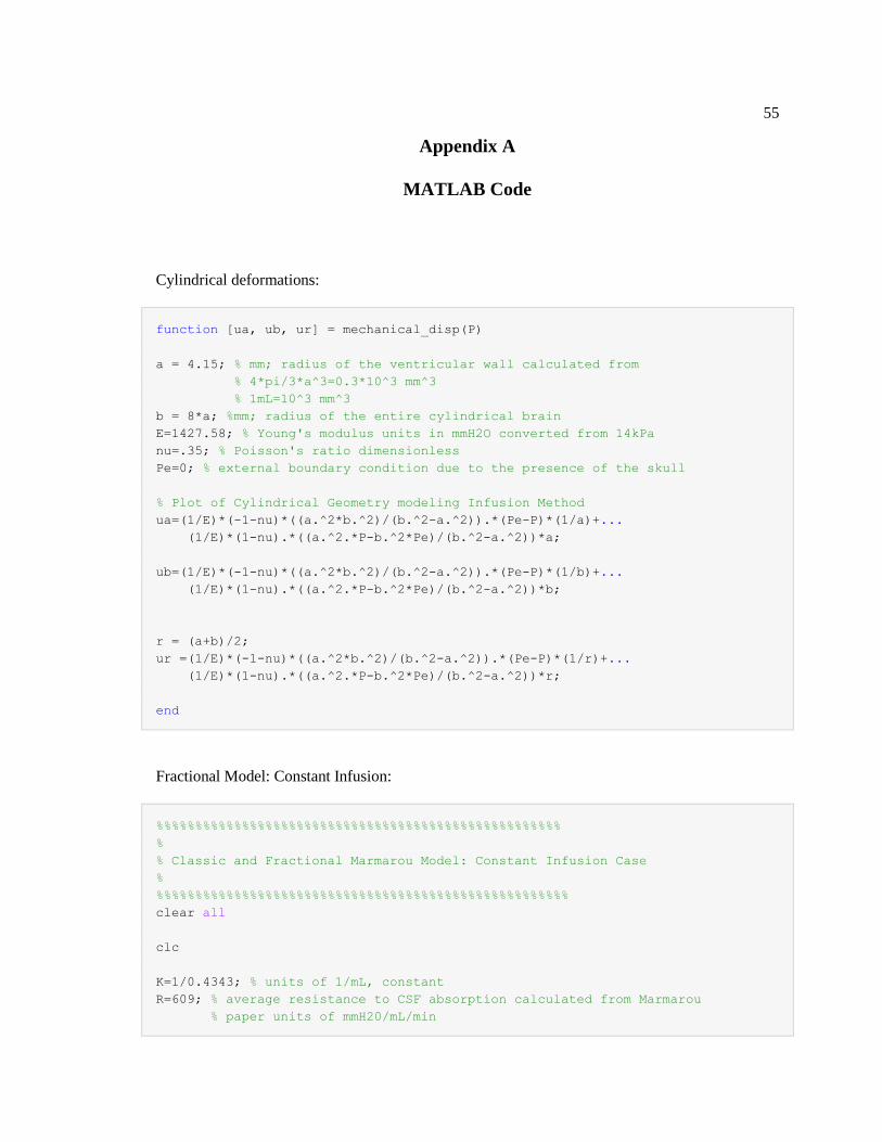
Cylindrical deformations:

function [ua, ub, ur] = mechanical_disp(P)

a = 4.15; % mm; radius of the ventricular wall calculated from

% 4*pi/3*a^3=0.3*10^3 mm^3

% 1mL=10^3 mm^3

b = 8*a; %mm; radius of the entire cylindrical brain

E=1427.58; % Young's modulus units in mmH2O converted from 14kPa

nu=.35; % Poisson's ratio dimensionless

Pe=0; % external boundary condition due to the presence of the skull

% Plot of Cylindrical Geometry modeling Infusion Method

ua=(1/E)*(-1-nu)*((a.^2*b.^2)/(b.^2-a.^2)).*(Pe-P)*(1/a)+...

(1/E)*(1-nu).*((a.^2.*P-b.^2*Pe)/(b.^2-a.^2))*a;

ub=(1/E)*(-1-nu)*((a.^2*b.^2)/(b.^2-a.^2)).*(Pe-P)*(1/b)+...

(1/E)*(1-nu).*((a.^2.*P-b.^2*Pe)/(b.^2-a.^2))*b;

r = (a+b)/2;

ur =(1/E)*(-1-nu)*((a.^2*b.^2)/(b.^2-a.^2)).*(Pe-P)*(1/r)+...

(1/E)*(1-nu).*((a.^2.*P-b.^2*Pe)/(b.^2-a.^2))*r;

end

Fractional Model: Constant Infusion:

%%%%%%%%%%%%%%%%%%%%%%%%%%%%%%%%%%%%%%%%%%%%%%%%%%%%

%

% Classic and Fractional Marmarou Model: Constant Infusion Case

%

%%%%%%%%%%%%%%%%%%%%%%%%%%%%%%%%%%%%%%%%%%%%%%%%%%%%%

clear all

clc

K=1/0.4343; % units of 1/mL, constant

R=609; % average resistance to CSF absorption calculated from Marmarou

% paper units of mmH20/mL/min

56

Po=100; % units of mmH2O, normal opening (starting pressure level)

F=.02; % change in I described in Marmarou

t=0:1:100; %t, time measured in minutes

%%%%%%%%%%%%%%%%%%%%%%%%%%%%%%%%

% constant C; linear ODES

%%%%%%%%%%%%%%%%%%%%%%%%%%%%%%%%

C = 1/K;

%%%%%%%%%%%%%%

% Classic case

%%%%%%%%%%%%%%

P_l_classic = Po+R*F-R*F*exp(-t/(C*R));

figure, plot(t,P_l_classic, 'k');

hold on;

%%%%%%%%%%%%%%%%%

% Fractional case

%%%%%%%%%%%%%%%%%

alpha = [0.25, 0.5, 0.75, 0.95];

for i = 1:4

a0 = Po;

a1(i) = 1/gamma(alpha(i)+1)*(F/C+Po/(C*R)-a0/(C*R));

a2(i) = gamma(alpha(i)+1)/gamma(2*alpha(i)+1)*(-a1(i))/(C*R);

a3(i) = gamma(2*alpha(i)+1)/gamma(3*alpha(i)+1)*(-a2(i))/(C*R);

a4(i) = gamma(3*alpha(i)+1)/gamma(4*alpha(i)+1)*(-a3(i))/(C*R);

P_l_frac(:,i) = a0+a1(i)*t.^alpha(i)+a2(i)*t.^(2*alpha(i))+...

a3(i)*t.^(3*alpha(i))+a4(i)*t.^(4*alpha(i));

end;

plot(t, P_l_frac(:,1), 'r', t, P_l_frac(:,2), 'm',...

t, P_l_frac(:,3), 'g', t, P_l_frac(:,4), 'b');

hold off;

xlabel('Time (min)');

ylabel('Pressure(Pa)');

title('Infusion Pressures - Linear Classic and Fractional Cases');

clear alpha a0 a1 a2 a3 a4

57

%%%%%%%%%%%%%%%%%%%%%%%%%%%%%%%%%%%%%

% nonlinear Ricatti ODES

%%%%%%%%%%%%%%%%%%%%%%%%%%%%%%%%%%%%%

%%%%%%%%%%%%%%%

% Classic case: Marmarou solution from his paper

%%%%%%%%%%%%%%%

P=(Po*(Po+R*F))./(Po+(R*F).*exp(-(K/R)*(Po+R*F).*t));

figure, plot(t,P, 'k');

hold on;

%%%%%%%%%%%%%%%%%

% Fractional case

%%%%%%%%%%%%%%%%%

alpha = [0.1, 0.25, 0.3, 0.35];

beta1 = -K*(F+Po/R);

beta2 = K/R;

for i = 1:4

a0 = Po;

A0 = a0^2;

a1(i) = 1/gamma(alpha(i)+1)*(-beta1*a0-beta2*A0);

A1(i) = 2*a0*a1(i);

a2(i) = gamma(alpha(i)+1)/gamma(2*alpha(i)+1)*(-beta1*a1(i)-beta2*A1(i));

A2(i) = a1(i)^2+2*a0*a2(i);

a3(i) = gamma(2*alpha(i)+1)/gamma(3*alpha(i)+1)*(-beta1*a2(i)-beta2*A2(i));

P_frac(:,i) = a0+a1(i)*t.^alpha(i)+a2(i)*t.^(2*alpha(i))+...

a3(i)*t.^(3*alpha(i));

rho(i) = 1/abs(a3(i))^(1/(3*alpha(i))); %radius of convergence

end;

plot(t, P_frac(:,1), 'r', t, P_frac(:,2), 'm',...

t, P_frac(:,3), 'g', t, P_frac(:,4), 'b');

hold off;

xlabel('Time (min)');

ylabel('Pressure (Pa)');

title('Infusion Pressures - Nonlinear Classic and Fractional Cases');

clear alpha a0 a1 a2 a3 A0 A1 A2

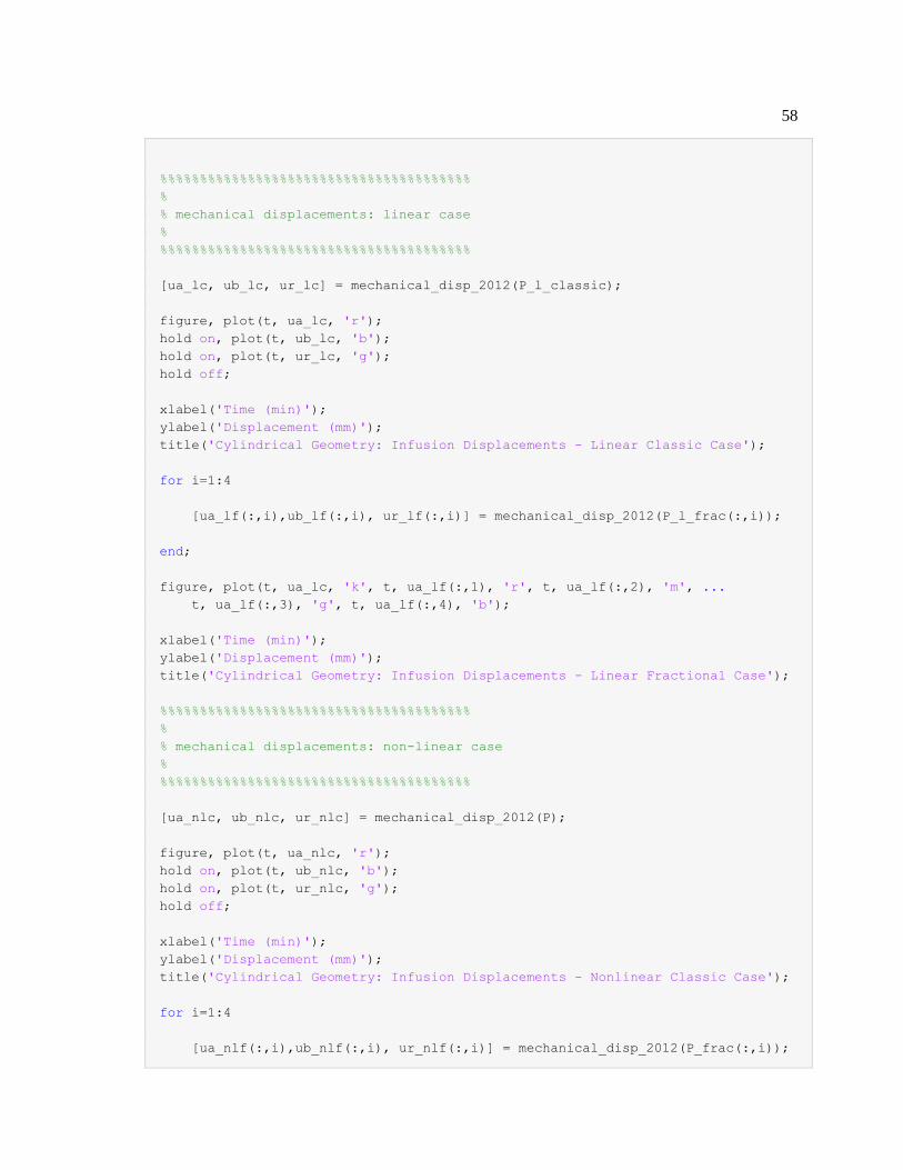
58

%%%%%%%%%%%%%%%%%%%%%%%%%%%%%%%%%%%%%%%

%

% mechanical displacements: linear case

%

%%%%%%%%%%%%%%%%%%%%%%%%%%%%%%%%%%%%%%%

[ua_lc, ub_lc, ur_lc] = mechanical_disp_2012(P_l_classic);

figure, plot(t, ua_lc, 'r');

hold on, plot(t, ub_lc, 'b');

hold on, plot(t, ur_lc, 'g');

hold off;

xlabel('Time (min)');

ylabel('Displacement (mm)');

title('Cylindrical Geometry: Infusion Displacements - Linear Classic Case');

for i=1:4

[ua_lf(:,i),ub_lf(:,i), ur_lf(:,i)] = mechanical_disp_2012(P_l_frac(:,i));

end;

figure, plot(t, ua_lc, 'k', t, ua_lf(:,1), 'r', t, ua_lf(:,2), 'm', ...

t, ua_lf(:,3), 'g', t, ua_lf(:,4), 'b');

xlabel('Time (min)');

ylabel('Displacement (mm)');

title('Cylindrical Geometry: Infusion Displacements - Linear Fractional Case');

%%%%%%%%%%%%%%%%%%%%%%%%%%%%%%%%%%%%%%%

%

% mechanical displacements: non-linear case

%

%%%%%%%%%%%%%%%%%%%%%%%%%%%%%%%%%%%%%%%

[ua_nlc, ub_nlc, ur_nlc] = mechanical_disp_2012(P);

figure, plot(t, ua_nlc, 'r');

hold on, plot(t, ub_nlc, 'b');

hold on, plot(t, ur_nlc, 'g');

hold off;

xlabel('Time (min)');

ylabel('Displacement (mm)');

title('Cylindrical Geometry: Infusion Displacements - Nonlinear Classic Case');

for i=1:4

[ua_nlf(:,i),ub_nlf(:,i), ur_nlf(:,i)] = mechanical_disp_2012(P_frac(:,i));

59

end;

figure, plot(t, ua_nlc, 'k', t, ua_nlf(:,1), 'r', t, ua_nlf(:,2), 'm', ...

t, ua_nlf(:,3), 'g', t, ua_nlf(:,4), 'b');

xlabel('Time (min)');

ylabel('Displacement (mm)');

title('Cylindrical Geometry: Infusion Displacements - Nonlinear Fractional

Case');

Fractional Model: Injection:

%%%%%%%%%%%%%%%%%%%%%%%%%%%%%%%%%%%%%%%%%%%%%%%%%%%%

%

% Classic and Fractional Marmarou Model: Bolus Injection Case

%

%%%%%%%%%%%%%%%%%%%%%%%%%%%%%%%%%%%%%%%%%%%%%%%%%%%%%

clear all

clc

K=1/0.4343; % units of 1/mL, constant

R=609; % average resistance to CSF absorption calculated from Marmarou

% paper units of mmH20/mL/min

Po=100; % units of mmH2O, normal opening (starting pressure level)

F=.02; % change in I described in Marmarou for cats

%V0 = 120; % units of mL, initial CSF volume in normal humans

V0 = 3; % units of mL, initial CSF volume in normal cats (approx)

V = 0.02; % added volume bolus CHECK THIS VALUE!

t= 0:0.05:1; %t, time measured in minutes

dt = 0.05;

%%%%%%%%%%%%%%%%%%%%%%

% Marmarou's solution: does NOT satisfy initial condition and the equation

% at t = 0!!!

P_marmarou = Po*exp(K*V)*exp(K*Po*t/R)./(1+exp(K*V)*(exp(K*Po*t/R)-1)); %

pressure

figure, plot(t,P_marmarou, 'k-', 'LineWidth', 2);

hold on;

60

%P_mysol = Po./(1-K*V*exp(-K*Po*t/R).*heaviside(t)); % this however is not

solving the same

% Marmarou equation!

%plot(t, P_mysol, 'rd', 'LineWidth', 1.2);

%hold off;

% use an approximation for Dirac distribution to find the solution to

% original Marmarou equation:

% let Dirac = lim (eps goes to 0) 1/2*eps*t^(eps-1)

eps = 1e-10;

Vol_numeric = zeros(length(t),1);

Vol_numeric(1) = V0;

Vol_marmarou = zeros(length(t),1);

Vol_marmarou(1) = V0;

dVdt_marmarou = -1/R*P_marmarou+V*1/2*eps.*t.^(eps-1)+Po/R;

%note the use of the approximation of Dirac distribution in dVdt_marmarou!

for i =1:length(t)

P_numeric(i) = exp(K*(1/2*V*t(i)^eps+Po/R*t(i)))/(1/Po+K/R*...

quad(@(tau)exp(K.*(1/2*V*tau.^eps+Po/R.*tau)),0,t(i)));

dVdt_numeric(i) = -1/R*P_numeric(i)+V*1/2*eps.*t(i)^(eps-1)+Po/R;

if (i > 1)

Vol_numeric(i) = Vol_numeric(i-1)+dVdt_numeric(i)*dt;

Vol_marmarou(i) = Vol_marmarou(i-1)+dVdt_numeric(i)*dt;

end;

end;

plot(t,P_numeric, 'b--', 'LineWidth', 2);

xlabel('Time (min)');

ylabel('CSF Pressure (mmH20)');

title('Pressure: Marmarou vs. corrected solution');

hold off;

figure, plot(t,Vol_numeric,'k-', t, Vol_marmarou, 'b--', 'LineWidth', 2);

xlabel('Time (min)');

ylabel('Volume (mL)');

title('Volume: Marmarou vs. corrected solution');

%%%%%%%%%%%%%%%%%%%%%%%%%

% linear case

61

P_l_classic = Po+K*V*exp(-K.*t/R).*heaviside(t);

figure, plot(t, P_l_classic, 'k', 'LineWidth', 2);

hold on;

alpha = [0.25, 0.5, 0.75, 0.95];

for i = 1:length(alpha)

P_l_frac(:,i) = Po+K*Po/R*(-1/gamma(alpha(i)+1)+...

1/(alpha(i)*gamma(alpha(i))))*t.^alpha(i)+...

K^2*Po/R^2*(1/gamma(2*alpha(i)+1)-...

1/(2*alpha(i)*gamma(2*alpha(i))))*t.^(2*alpha(i))+...

K*V/gamma(alpha(i)).*t.^(alpha(i)-1)-...

K/R*K*V/gamma(2*alpha(i)).*t.^(2*alpha(i)-1)+...

K^2/R^2*K*V/gamma(3*alpha(i)).*t.^(3*alpha(i)-1); % fractional

pressure

end;

P_l_frac(1,:) = Po; % there is an issue in the for loop with t(1)^(alpha-1)

% giving NaN since t(1)=0

plot(t, P_l_frac(:,1), 'r', t, P_l_frac(:,2), 'm',...

t, P_l_frac(:,3), 'g', t, P_l_frac(:,4), 'b', 'LineWidth', 2);

xlabel('Time (min)');

ylabel('CSF Pressure (mmH20)');

title('CSF Pressure - Classic and Fractional Linear Case')

hold off;

%%%%%%%%%%%%%%%%%%%%%%%%%%%%%%%%%%%%%%%

%

% mechanical displacements: linear case

%

%%%%%%%%%%%%%%%%%%%%%%%%%%%%%%%%%%%%%%%

[ua_lc, ub_lc, ur_lc] = mechanical_disp(P_l_classic);

for i=1:4

[ua_lf(:,i),ub_lf(:,i), ur_lf(:,i)] = mechanical_disp(P_l_frac(:,i));

end;

figure, plot(t, ua_lf(:,1), 'k-.', t, ua_lf(:,2), 'k+-',...

t, ua_lf(:,3), 'k*-', t, ua_lf(:,4), 'k--',...

t, ua_lc, 'k', 'LineWidth', 2);

xlabel('Time (min)');

ylabel('Displacement (mm)');

62

title('Cylindrical Geometry: Displacement - Classic vs. Fractional Linear

Case');

%%%%%%%%%%%%%%%%%%%%%%%%%%%%

% non-linear case

%

% use an approximation for Dirac distribution to find the solution to

% our fractional model; cannot use the same approximation as before, namely

% Dirac = lim (eps goes to 0) 1/2*eps*t^(eps-1), due to a singularity at 0

% in an integral we have to evaluate. thus we take for this case the

% following approximation:

% Dirac = lim (eps goes to 0) 1/(2*sqrt(pi*eps))*exp(-x^2/(4*eps))

tt = 1;

Vol_nl_frac_numeric = zeros(length(t),length(alpha));

Vol_nl_frac_numeric(1,:) = V0;

for j = 1:length(alpha)

h1(j) = 1/(gamma(alpha(j)+1)*gamma(1-alpha(j)))*(-

1/(4*eps*sqrt(eps*pi)))*...

fgauss_integr(@(s)s.*exp(-s.^2./(4*eps))./(tt-s).^alpha(j),0,tt,4);

% h1 is a limit as eps goes to 0 and tt goes to 0, too!!

P_nl_frac_numeric(:,j) = Po + K*V*Po/(gamma(alpha(j)+1)).*t.^alpha(j)+...

K*V*Po/(gamma(2*alpha(j)+1))*(K*V - K*Po/R +

gamma(alpha(j)+1)*h1(j)).*...

t.^(2*alpha(j));

for i =1:length(t)

dVdt_nl_frac_numeric(i,j) = -1/R*P_nl_frac_numeric(i,j)+...

V*1/(2*sqrt(pi*eps))*exp(-t(i)^2/(4*eps))+Po/R;

if (i > 1)

Vol_nl_frac_numeric(i,j) = Vol_nl_frac_numeric(i-1,j)+...

dVdt_nl_frac_numeric(i,j)*dt;

end;

end;

rho(j) = 1/abs(K*V*Po/(gamma(2*alpha(j)+1))*(K*V - K*Po/R +...

gamma(alpha(j)+1)*h1(j)))^(1/(2*alpha(j))) %radius of convergence

end;

figure, plot(t, P_nl_frac_numeric(:,1), 'k-.',t, P_nl_frac_numeric(:,2), 'k+-

',...

t, P_nl_frac_numeric(:,3), 'k*-', t, P_nl_frac_numeric(:,4), 'k--',...

63

t, P_numeric, 'k', 'LineWidth', 1.2);

xlabel('Time (min)');

ylabel('CSF Pressure (mmH20)');

%title('CSF Pressure - Classic and Fractional Non-Linear Case')

figure, plot(t, Vol_nl_frac_numeric(:,1), 'k-.', t, Vol_nl_frac_numeric(:,2),

'k+-',...

t, Vol_nl_frac_numeric(:,3), 'k*-', t, Vol_nl_frac_numeric(:,4), 'k--',...

t, Vol_numeric, 'k', 'LineWidth', 1.2);

xlabel('Time (min)');

ylabel('Volume (mL)');

%title('Volume: Classic vs. Fractional Nonlinear Case');

%%%%%%%%%%%%%%%%%%%%%%%%%%%%%%%%%%%%%%%

%

% mechanical displacements: non-linear case

%

%%%%%%%%%%%%%%%%%%%%%%%%%%%%%%%%%%%%%%%

for i = 1:length(t)

[ua_nlc(i), ub_nlc(i), ur_nlc(i)] = mechanical_disp(P_numeric(i));

end;

[ua_marmarou, ub_marmarou, ur_marmarou] = mechanical_disp(P_marmarou);

figure, plot(t, ua_nlc, 'k', t, ua_marmarou, 'ko', 'LineWidth',2);

hold on, plot(t, ub_nlc, 'b', t, ub_marmarou, 'bo', 'LineWidth',2);

hold on, plot(t, ur_nlc, 'r', t, ur_marmarou, 'ro', 'LineWidth',2);

hold off;

xlabel('Time (min)');

ylabel('Displacement (mm)');

title('Cylindrical Geometry: Displacement - Nonlinear Classic Case');

for i=1:4

[ua_nlf(:,i),ub_nlf(:,i), ur_nlf(:,i)] =

mechanical_disp(P_nl_frac_numeric(:,i));

end;

figure, plot(t, ua_nlf(:,1), 'k-.', t, ua_nlf(:,2), 'k+-',...

t, ua_nlf(:,3), 'k*-', t, ua_nlf(:,4), 'k--',...

t, ua_nlc, 'k', 'LineWidth', 2);

xlabel('Time (min)');

ylabel('Displacement (mm)');

title('Cylindrical Geometry: Displacement - Classic vs. Fractional Nonlinear

Case');

Brain Data: Normal:

64

function dbN = brainN( t, bN )

dbN = zeros(4,1);

epsilon = 1;

dbN(1) = bN(3);

dbN(2) = bN(4);

dbN(3) = -(-0.0001*t^2+0.0098*t+0.8435-1)^2*(1-epsilon*bN(2));

dbN(4) = epsilon*(-0.0001*t^2+0.0098*t+0.8435-1)^2*bN(1);

end

Brain Data: Hydrocephalic:

function dbH = brainH( t, bH )

dbH = zeros(4,1);

epsilon = 1;

dbH(1) = bH(3);

dbH(2) = bH(4);

dbH(3) = -(-0.0004*t^2+0.0482*t+0.2792-1)^2*(1-epsilon*bH(2));

dbH(4) = epsilon*(-0.0004*t^2+0.0482*t+0.2792-1)^2*bH(1);

end

Hamilton’s Principle Model

clear all

%use Mandell et al, 2010 data in table 1 for brain volumes of normal and

%

%hydrocephalic mice

xy_normal = load('brainJ_normal_vol_mice.m');

time_normal = xy_normal(:,1);

vol_normal = xy_normal(:,2);

%plot(time_normal, vol_normal, 'ro', 'LineWidth', 2);

pn = polyfit(time_normal, vol_normal, 2);

%hold on;

65

%plot (time_normal, pn(1).*time_normal.^2+pn(2).*time_normal+pn(3), 'k-',

'LineWidth', 2);

%hold off;

%%%%%%%%%%%%%%%%%%%%%%%%%%%%%%

xy_hydro = load('brainJ_hydrocephalus_vol_mice.m');

time_hydro = xy_hydro(:,1);

vol_hydro = xy_hydro(:,2);

%figure, plot(time_hydro, vol_hydro, 'bo');

ph = polyfit(time_hydro, vol_hydro, 2);

%hold on;

%plot (time_hydro, ph(1).*time_hydro.^2 + ph(2).*time_hydro + ph(3), 'k-',

'LineWidth', 2);

%hold off;

%%%%%%%%%%%%%%%%%%%%%%%%%%%%%%

% the system of ODEs is however stiff so dsolve can find the analytic

% solutions but they are very poorly behavied; try numerical solutions

[tN100eps, bN100eps] = ode45(@brainN, [18 85], [1 0 0 eps]);

[tH100eps, bH100eps] = ode45(@brainH, [18 85], [1 0 0 eps]);

[tN101eps, bN101eps] = ode45(@brainN, [18 85], [1 0 0.1 eps]);

[tH101eps, bH101eps] = ode45(@brainH, [18 85], [1 0 0.1 eps]);

[tN01m11, bN01m11] = ode45(@brainN, [18 85], [0 1 -1 1]);

[tH01m11, bH01m11] = ode45(@brainH, [18 85], [0 1 -1 1]);

figure,

subplot(3,2,1)

plot(tN100eps, bN100eps(:,1), 'r', tN100eps, bN100eps(:,2), 'b', 'LineWidth',

2);

xlabel('a)');

subplot(3,2,2)

plot(tH100eps, bH100eps(:,1), 'r', tH100eps, bH100eps(:,2), 'b', 'LineWidth',

2);

xlabel('b)');

subplot(3,2,3)

plot(tN101eps, bN101eps(:,1), 'r', tN101eps, bN101eps(:,2), 'b', 'LineWidth',

2);

xlabel('c)');

66

subplot(3,2,4)

plot(tH101eps, bH101eps(:,1), 'r', tH101eps, bH101eps(:,2), 'b', 'LineWidth',

2);

xlabel('d)');

subplot(3,2,5)

plot(tN01m11, bN01m11(:,1), 'r', tN01m11, bN01m11(:,2), 'b', 'LineWidth', 2);

xlabel('e)');

subplot(3,2,6)

plot(tH01m11, bH01m11(:,1), 'r', tH01m11, bH01m11(:,2), 'b', 'LineWidth', 2);

xlabel('f)');

[ax1,h1]=suplabel('Time (days)');

[ax2,h2]=suplabel('Growth and Inflammation States','y');

%

%figure, plot(tN, bN(:,3), 'r', tN, bN(:,4), 'b', 'LineWidth', 2);

%

%figure, plot(tH, bH(:,3), 'r', tH, bH(:,4), 'b', 'LineWidth', 2);

%

67

Bibliography

1. Marmarou, A., Shulman, K., & Rosende, R. M. (1978). A nonlinear analysis of the

cerebrospinal fluid system and intracranial pressure dynamics. Surgical Neurology, 48,

332-344.

2. Hakim, S., Venegas, J. G., & Burton, J. D. (1976). The Physics of the cranial cavity,

hydrocephalus and normal pressure hydrocephalus: Mechanical interpretation and

mathermatical model. Surgical Neurology(5), 187-210.

3. Duan, J.-S., Chaolu, T., & Rach, R. (2012). Solutions of the initial value problem for

nonlinear fractional ordinary differential equations by the Rach-Adomian-Meyers

modified decomposition method. Applied Mathematics and Computation, 218, 8370-

8392.

4. Kauffman J.,Drapaca C.S. (2013). A Multiscale Pressure-Volume model of Cerebrospinal

Fluid Dynamics: Application to Hydrocephalus. Proceedings of the ASME 2012 2nd

Global Congress on Nanoengineering for Medicine & Biology NEMB 2013.

5. Kauffman J., Drapaca C.S. (2013). A Fractional Pressure- Volume Model of

Cerebrospinal Fluid Dynamics in Hydrocephalus. Proceedings of the Annual Conference

& Exposition on Experimental and Applied Mechanics SEM 2013.

6. Drapaca C.S., Kauffman J.A. (2013). A Study of Brain Biomechanics using Hamilton’s

Principle. Interdisciplinary Conference Series: Applied Mathematics, Modeling, and

Computer Science AMMC2013.

7. Kauffman, J. A. (2012). Simulation of hydrocephalus based on mathematical modeling

and technological advancements.Honors Thesis, The Pennsylvania State University.

68

8. Czosnyka, M., Czosnyka, Z., Momjian, S., & Pickard, J. D. (2004). Cerebrospinal fluid

dynamics. Physiological Measurement, 25(5).

9. “Hydrocephalus Association: Brain physiology webpage”.

URL http://www.hydroassoc.org/hydrocephalus-education-and-support/learning-about-

hydrcephalus/brain-physiology-relevant-to-hydrocephalus/

10. Weerakkody, R. A., Czosnyka, M., Schuhmann, M. U., Schmidt, E., Keong, N., &

Santarius, T. (2011). Clinical Assessment of cerebrospinal fluid dynamics in

hydrocephalus: guide to interpretation based on observational study. Acta Neurologica

Scandinavica, 124, 85-98.

11. Iliff, J. J., Wang, M., Liao, Y., Plogg, B.A., Peng, W., Gundersen G.A., Benveniste, H.,

Vates, G.E., Deane, R., & Goldman, S.A. (2012). Facilitates CSF Flow Through the

Brain Parenchyma and the Clearance of the Interstitial Solutes, Including Amyloid.

Science Translational Medicine,4,p.147ra111.

12. Lundstorm, B. N., Higgs, M. H., Spain, W. J., & Fairhall, A. L. (2008). Fractional

differentiation by neocoritcal pyramidal neurons. Nature Neuroscience, 11, 1335-1342.

13. Sherief, H. H., El-Sayed, A., Behiry, S. H., & Raslan, W. E. (2012). Using Fractional

Derivatives to Generalize the Hodgkin-Huxley Model. (D. Baleanu, J. Machado, & A.

Luo, Eds.) New York: Springer.

14. Adomian, G. (1995). Solving the mathematical models of neurosciences and medicine.

Mathematics and Computers in Simulation, 40, 107-114.

15. Momani, S., & Shawagfeh, N. (2006). Decomposition method for solving fractional

Riccati differential equations. Applied Mathematics and Computation, 182, 1083-1092.

16. Odibat, Z. M., & Shawagfeh, N. T. (2007). Generalized Taylor's Formula. Appl. Math.

Comp.(186), 286-293.

69

17. Timoshenko, S., Goodier, J.N. (1970). Theory of Elasticity (3rd ed.). McGraw-Hill Book

Company.

18. Brunelle, F. (2004). Modern Imaging of Pediatric Hydrocephalus. In Pediatric

Hydrocephalus (pp. 79-94).

19. Singh, T., & Newman, A. (2011). Inflammatory markers in population studies of aging.

Ageing Res.Rev, 10(3), 319-329.

20. Cusumano, J., Roy, A., & Li, Q. (In Preparation). Damage Dynamics, rate laws, and

failure statistics via Hamilton's principle. Royal Society A.

21. Fried, E., & Gurtin, M. (1993). Continuum theory of themally induced phase transitinos

based on an order parameter. Physica D(68), 326-343.

22. Fried, E., & Gurtin, M. (1994). Dynamics solid-solid transitions with phase characterized

by an order parameter. Physica D.(72), 287-308.

23. Mandell, J., Neuberger, T., Drapaca, C., Webb, A., & Schiff, S. (2010). The dynamics of

brain and cerebrospinal fluid growth in normal versus hydrocephalic mice. J. Neurosurg.

Pediatrics(6), 1-10.

24. Ibragimov, A., Ritter, L., & Walton, J. R. (2010). Stability Analysis of a Reaction-

Diffusion System Modeling Atherogenesis. Journal of Applied Mathematics, 70, 2150-

2185.

25. Zheng , W., & Chodobski, A. (2005). The Blood-Cerebrospinal Fluid Barrier. Boca

Raton, FL: Taylor and Francis Group.