mathematical and computational methods in …mathematical and computational methods in photonics and...
TRANSCRIPT

Mathematical and Computational Methods
in Photonics and Phononics
H. Ammari and B. Fitzpatrick and H. Kang and M. Ruiz and S. Yu and
H. Zhang
Research Report No. 2017-05
January 2017Latest revision: March 2017
Seminar für Angewandte MathematikEidgenössische Technische Hochschule
CH-8092 ZürichSwitzerland
____________________________________________________________________________________________________

Mathematical and Computational Methods in
Photonics and Phononics
Habib Ammari
Brian Fitzpatrick
Hyeonbae Kang
Matias Ruiz
Sanghyeon Yu
Hai Zhang
Department of Mathematics, ETH Zurich, Ramistrasse 101, CH-
8092 Zurich, Switzerland
E-mail address: [email protected]
Department of Mathematics, ETH Zurich, Ramistrasse 101, CH-
8092 Zurich, Switzerland
E-mail address: [email protected]
Department of Mathematics, Inha University, Incheon 402-751, Ko-
rea
E-mail address: [email protected]
Department of Mathematics and Applications, Ecole Normale Superieure,
45 Rue d’Ulm, 75005 Paris, France
E-mail address: [email protected]
Department of Mathematics, ETH Zurich, Ramistrasse 101, CH-
8092 Zurich, Switzerland
E-mail address: [email protected]
Department of Mathematics, HKUST, Clear Water Bay, Kowloon,
Hong Kong
E-mail address: [email protected]

1991 Mathematics Subject Classification. 47A55, 47A75, 31A10, 34A55, 35R30,35B34, 45Q05, 30E25
Key words and phrases. nanophotonics, diffractive optics, photonic crystals,plasmonic resonance, Minnaert bubble, Helmholtz resonator, metamaterials,
superresolution, subwavelength resonator, electromagnetic invisibility, cloaking,layer potentials, asymptotic analysis, Gohberg-Sigal’s theory.
Abstract. The fields of photonics and phononics encompass the fundamentalscience of light and sound propagation and interactions in complex structures,and its technological applications. The aim of this book is to review newand fundamental mathematical tools, computational approaches, and inver-sion and optimal design methods to address challenging problems in photon-
ics and phononics. An emphasis is placed on analyzing subwavelength res-onators; super-focusing and super-resolution of electromagnetic and acoustic
waves; photonic and phononic crystals; electromagnetic cloaking; and electro-magnetic and elastic metamaterials and metasurfaces. Throughout this book,we demonstrate the power of layer potential techniques for solving challengingproblems in photonics and phononics when they are combined with asymptoticanalysis. The book could be of interest to researchers and graduate studentsworking in the fields of applied and computational mathematics, partial dif-ferential equations, electromagnetic theory, elasticity, integral equations, andinverse and optimal design problems in photonics and phononics. Researchersin nanotechnologies might also find this book helpful.

Contents
Introduction 1
Part 1. Mathematical and Computational Tools 5
Chapter 1. Generalized Argument Principleand Rouche’s Theorem 7
1.1. Introduction 71.2. Argument Principle and Rouche Theorem 71.3. Definitions and Preliminaries 81.4. Factorization of Operators 111.5. Main Results of the Gohberg and Sigal Theory 121.6. Muller’s Method 161.7. Concluding Remarks 17
Chapter 2. Layer Potentials 192.1. Introduction 192.2. Sobolev Spaces 192.3. Layer Potentials for the Laplace Equation 212.4. Neumann–Poincare Operator 232.5. Conductivity Problem in Free Space 392.6. Periodic and Quasi-Periodic Green’s Functions 532.7. Shape Derivatives of Layer Potentials 622.8. Layer Potentials for the Helmholtz Equation 672.9. Laplace Eigenvalues 752.10. Helmholtz-Kirchhoff Identity, Scattering Amplitude and Optical
Theorem 852.11. Scalar Wave Scattering by Small Particles 962.12. Quasi-Periodic Layer Potentials for the Helmholtz Equation 1032.13. Computations of Periodic Green’s Functions 1072.14. Integral Representation of Solutions to the Full Maxwell Equations 1172.15. Integral Representation of Solutions to the Lame System 1382.16. Quasi-Periodic Layer Potentials for the Lame System 1682.17. Concluding Remarks 170
Chapter 3. Perturbations of Cavities and Resonators 1713.1. Introduction 1713.2. Optical Cavities 1713.3. Optical Resonators 1833.4. Elastic Cavities 1853.5. Eigenvalue Perturbations Due to Shape Deformations 192
v
vi CONTENTS
3.6. Concluding Remarks 193
Part 2. Diffraction Gratings and Band-Gap Materials 195
Chapter 4. Diffraction Gratings 1974.1. Introduction 1974.2. Electromagnetic Theory of Gratings 1974.3. Variational Formulations 2054.4. Boundary Integral Formulations 2234.5. Optimal Design of Grating Profiles 2254.6. Numerical Implementation 2264.7. Concluding Remarks 228
Chapter 5. Photonic Band Gaps 2295.1. Introduction 2295.2. Floquet Transform 2305.3. Structure of Spectra of Periodic Elliptic Operators 2305.4. Boundary Integral Formulation 2315.5. Sensitivity Analysis with Respect to the Index Ratio 2415.6. Photonic Band Gap Opening 2505.7. Sensitivity Analysis with Respect to Small Perturbations in the
Geometry of the Holes 2515.8. Proof of the Representation Formula 252
5.9. Characterization of the Eigenvalues of ∆ 2545.10. Maximizing Band Gaps in Photonic Crystals 2545.11. Photonic Cavities 2565.12. Concluding Remarks 257
Chapter 6. Phononic Band Gaps 2596.1. Introduction 2596.2. Asymptotic Behavior of Phononic Band Gaps 2606.3. Criterion for Gap Opening 2776.4. Gap Opening Criterion When Densities Are Different 2806.5. Concluding Remarks 282
Part 3. Subwavelength Resonant Structures and Super-resolution 283
Chapter 7. Plasmonic Resonances for Nanoparticles 2857.1. Introduction 2857.2. Quasi-Static Plasmonic Resonances 2867.3. Effective Medium Theory for Suspensions of Plasmonic Nanoparticles 2887.4. Shift in Plasmonic Resonances Due to the Particle Size 2927.5. Plasmonic Resonance for a System of Spheres 3007.6. Concluding Remarks 307
Chapter 8. Imaging of Small Particles 3098.1. Introduction 3098.2. Scalar Wave Imaging of Small Particles 3098.3. Electromagnetic Imaging 3138.4. Elasticity Imaging 313

CONTENTS vii
8.5. Numerical Illustrations 3168.6. Concluding Remarks 316
Chapter 9. Super-Resolution Imaging 3199.1. Introduction 3199.2. Super-Resolution Imaging in High-Contrast Media 3199.3. Super-Resolution in Resonant Structures 3309.4. Super-Resolution Based on Scattering Tensors 3449.5. Concluding Remarks 345
Part 4. Metamaterials 347
Chapter 10. Near-Cloaking 34910.1. Introduction 34910.2. Near-Cloaking in the Quasi-Static Limit 35010.3. Near-Cloaking for the Helmholtz Equation 35310.4. Near-Cloaking for the Full Maxwell Equations 36110.5. Near-Cloaking for the Elasticity System 36710.6. Concluding Remarks 374
Chapter 11. Anomalous Resonance Cloaking and Shielding 37511.1. Introduction 37511.2. Layer Potential Formulation 37711.3. Anomalous Resonance in an Annulus 37911.4. Shielding at a Distance 38411.5. Concluding Remarks 391
Chapter 12. Plasmonic Metasurfaces 39512.1. Introduction 39512.2. Setting of the Problem 39612.3. Boundary-Layer Corrector and Effective Impedance 39712.4. Numerical Illustrations 40112.5. Concluding Remarks 402
Part 5. Subwavelength Phononics 405
Chapter 13. Helmholtz Resonator 40713.1. Introduction 40713.2. Hilbert Transform 40713.3. Perturbations of Scattering Frequencies of a Helmholtz Resonator 41213.4. Resonances of a System of Helmholtz Resonators and Super-
Resolution 41613.5. Concluding Remarks 419
Chapter 14. Minnaert Resonances for Bubbles 42114.1. Introduction 42114.2. Derivation of Minnaert Resonance Formula 42214.3. Effective Medium Theory for a System of Bubbles and Super-
Resolution 43014.4. Subwavelength Phononic Bandgap Opening 444

viii CONTENTS
14.5. Numerical Illustrations 45114.6. Concluding Remarks 455
Appendices A. Spectrum of Self-Adjoint Operators 457
Appendices B. Optimal Control and Level Set Representation 461B.1. Optimal Control Scheme 461B.2. Level Set Method 461B.3. Shape Derivatives 463
Bibliography 465
Index 483

Introduction
The aim of this book is to give a self-contained presentation of recent math-ematical and computational advances in photonics and phononics. The fields ofphotonics and phononics encompass the fundamental science of light and elasticwave propagation and interactions in complex structures, and its technological ap-plications.
The recent advances in nanoscience present great challenges for the applied andcomputational mathematics community. In nanophotonics, the aim is to control,manipulate, reshape, guide, and focus electromagnetic waves at nanometer lengthscales, beyond the resolution limit. In particular, one wants to push the resolutionlimit by reducing the focal spot and confining light to length scales significantlysmaller than half the wavelength. Nanostructures also open exciting opportunitiesfor tuning the phonon energy spectrum and related acoustic material properties forspecific applications.
Interactions between the field of photonics and mathematics has led to theemergence of a multitude of new and unique solutions in which today’s conventionaltechnologies are approaching their limits in terms of speed, capacity and accuracy.
Light can be used for detection and measurement in a fast, sensitive and ac-curate manner, and thus photonics possesses a unique potential to revolutionizehealthcare. Light-based technologies can be used effectively for very early detec-tion of diseases, with non-invasive imaging techniques or point-of-care applications.They are also instrumental in the analysis of processes at the molecular level, giv-ing a greater understanding of the origin of diseases, and hence allowing preventionalong with new treatments.
Photonic technologies also play a major role in addressing the needs of ourageing society: from pace-makers to synthetic bones and from endoscopes to themicro-cameras used in in-vivo processes. Photonics are used also in advanced light-ing technology and in improving energy efficiency and quality.
Specialized phononic crystals are currently being developed. These are artificialelastic structures with unusual acoustic wave propagation capabilities, such as theability to increase the resolution of ultrasound imaging with super lenses, or toprocess information with sound-based circuits.
By using photonic and phononic media to control waves across a wide bandof wavelengths, we have unprecedented ability to fabricate new optical and elasticmaterials with specific microstructures. Modern technologies are certainly going tobe based on the manipulation of electrons and photons.
Our main objective in this book is to report on the use of sophisticated math-ematics in diffractive optics, plasmonics, super-resolution, photonic and phononiccrystals, and metamaterials for electromagnetic and elastic invisibility and cloaking.
1

2 INTRODUCTION
We develop new mathematical and computational models for wave scatteringfrom sub-wavelength resonators and introduce a unified approach for designing,at low frequencies, metamaterials for cloaking and high-contrast media for sub-wavelength resolution. We establish sub-wavelength imaging approaches based onthe use of resonant plasmonic nanoparticles and Minnaert bubbles. By analyzingthe mathematical properties of sub-wavelength resonators, we unify the theoriesof metamaterials and super-focusing. This has certainly paved the way for thereshaping, controlling, and manipulation of waves at sub-wavelength scales.
The book merges various branches of mathematics to advance the field of math-ematical modelling of optical and acoustic subwavelength devices and structurescapable of light enhancement, and of the focusing and guiding of light at a subwave-length scale. These include asymptotic analysis, spectral analysis, and harmonicanalysis.
In particular, the book shows how powerful the layer potential techniques arefor solving challenging problems in photonics and phononics, especially when theyare combined with asymptotic analysis and the elegant theory of Gohberg and Sigalon meromorphic operator-valued functions.
The emerging discipline of phononics encompasses many disciplines, includingquantum physics and mechanics, material science, engineering, and applied math-ematics. The emphasis of this book is placed on mathematically analyzing plas-mon resonant nanoparticles and Minnaert bubbles, diffractive optics, photonic andphononic crystals, super-resolution, and metamaterials. For each of these topics, asolid mathematical and computational framework and an optimal design approachin the sense of robustness and accuracy is derived.
Plasmon resonant nanoparticles have unique capabilities of enhancing the bright-ness of light and confining strong electromagnetic fields. A reason for the thrivinginterest in optical studies of plasmon resonant nanoparticles is due to their re-cently proposed use as labels for molecular biology. New types of cancer diagnosticnanoparticles are constantly being developed.
A distinctive feature of bubbles in fluid is the high contrast between the airdensity inside and outside of the bubble. This results in a quasi-static acousticresonance, called the Minnaert resonance. At or near this resonant frequency, thesize of the bubble can be three orders of magnitude smaller than the wavelengthof the incident wave and the bubble behaves as a very strong monopole scattererof sound. The resonance makes the bubble a good candidate for acoustic sub-wavelength resonator. Bubbles have the potential to be the basic building blocksnot only for sub-wavelength acoustic imaging but also for acoustic meta-materials.
Super-resolution involves pushing the diffraction limits by reducing the focalspot size. Super-focusing is the counterpart of super-resolution. It describes elec-tromagnetic, acoustic or elastic waves to be confined to a length scale significantlysmaller than the diffraction limit of the focused waves. The super-focusing phenom-enon is being intensively investigated in the field of nanophotonics as a techniquewith the potential to focus electromagnetic radiation in a region of order of a fewnanometers beyond the diffraction limit of light and thereby causing an extraordi-nary enhancement of the electromagnetic field.
Plasmon resonant nanoparticles and Minnaert bubbles provide possible meansof achieving super-resolved imaging in biophotonics. In this book, we study the

INTRODUCTION 3
resonant property of high-contrast particles for different particle geometries andenvironments, and use them to achieve super-focusing and super-resolution.
Diffractive optics is a fundamental and vigorously growing technology whichcontinues to be a source of novel optical devices. Recent significant technologicaldevelopments of high precision micromachining techniques have permitted the cre-ation of gratings (periodic structures) and other diffractive structures with tiny fea-tures. Current and potential application areas include corrective lenses, microsen-sors, optical storage systems, optical computing and communication components,and integrated opto-electronic semiconductor devices.
Because of the small structural features, light propagation in micro-opticalstructures is generally governed by diffraction. In order to accurately predict theenergy distribution of an incident field in a given structure, the numerical solutionof the governing equation is required. If the field configurations are built up ofharmonic electromagnetic waves that are transverse, then the Maxwell equationscan be reduced to two scalar Helmholtz equations.
Throughout this book, we will focus on this scalar model and address signif-icant developments in mathematical analysis and modeling of diffractive optics.Particular emphasis is placed on the formulation of the mathematical model; well-posedness and regularity analysis of the solutions of governing equations in gratings;and optimal design and inverse diffraction problems in diffractive optics.
Photonic and phononic crystals are structures constructed of electromagneticand elastic materials arranged in a periodic array. They have attracted enormousinterest in the last decade because of their unique electromagnetic or elastic prop-erties. Such structures have been found to exhibit interesting spectral propertieswith respect to classical wave propagation, including the appearance of band gaps[281, 419, 462]. In this book, we construct subwavelength photonic and phononiccrystals using plasmonic particles and Minnaert bubbles.
Electromagnetic and elasticity invisibility is to render a target invisible to elec-tromagnetic and elastic probing. In this book, we investigate many schemes. Basedon a new effective medium theory for subwavelength resonators, we also provide amathematical framework for electromagnetic and elastic metamaterials.
The bibliography provides a list of relevant references. It is by no means com-prehensive. However, it should provide the reader with some useful guidance insearching for further details on the main ideas and approaches discussed in thisbook.
The material in this book is taught as a graduate course in applied mathemat-ics at ETH. Tutorial notes and Matlab codes can be downloaded at Codes. Some ofthe material in this book is from our wonderful collaborations with Toufic Abboud,Gang Bao, Giulio Ciraolo, Josselin Garnier, David Gontier, Vincent Jugnon, Hyun-dae Lee, Mikyoung Lim, Pierre Millien, Graeme Milton, Jean-Claude Nedelec, FadilSantosa, Michael Vogelius, and Darko Volkov. We feel indebted to all of them.


Part 1
Mathematical and Computational
Tools

CHAPTER 1
Generalized Argument Principle
and Rouche’s Theorem
1.1. Introduction
In this chapter we review the results of Gohberg and Sigal in [240] concerningthe generalization to operator-valued functions of two classical results in complexanalysis, the argument principle and Rouche’s theorem. An efficient and reliablemethod, referred to as Muller’s method, for finding a zero of a function definedon the complex plane is presented. This numerical method can be used for com-puting poles of integral operators, in particular for the computation of resonantcavities, band gap structures, and plasmonic resonances in nanoparticles. The re-sults described in this chapter will be applied to the mathematical theory of cavities,plasmonic nanoparticles, and photonic and phononic crystals.
1.2. Argument Principle and Rouche Theorem
To state the argument principle, we first observe that if f is holomorphic andhas a zero of order n at z0, we can write f(z) = (z−z0)ng(z), where g is holomorphicand nowhere vanishing in a neighborhood of z0, and therefore
f ′(z)f(z)
=n
z − z0+g′(z)g(z)
.
Then the function f ′/f has a simple pole with residue n at z0. A similar fact alsoholds if f has a pole of order n at z0, that is, if f(z) = (z − z0)
−nh(z), where h isholomorphic and nowhere vanishing in a neighborhood of z0. Then
f ′(z)f(z)
= − n
z − z0+h′(z)h(z)
.
Therefore, if f is meromorphic, the function f ′/f will have simple poles at the zerosand poles of f , and the residue is simply the order of the zero of f or the negativeof the order of the pole of f .
The argument principle results from an application of the residue formula. Itasserts the following.
Theorem 1.1 (Argument principle). Let V ⊂ C be a bounded domain withsmooth boundary ∂V positively oriented and let f(z) be a meromorphic function ina neighborhood of V . Let P and N be the number of poles and zeros of f in V ,counted with their orders. If f has no poles and never vanishes on ∂V , then
(1.1)1
2π√−1
∫
∂V
f ′(z)f(z)
dz = N − P.
7

8 1. GENERALIZED ARGUMENT PRINCIPLE AND ROUCHE’S THEOREM
Rouche’s theorem is a consequence of the argument principle [442]. It is insome sense a continuity statement. It says that a holomorphic function can beperturbed slightly without changing the number of its zeros. It reads as follows.
Theorem 1.2 (Rouche’s theorem). With V as above, suppose that f(z) andg(z) are holomorphic in a neighborhood of V . If |f(z)| > |g(z)| for all z ∈ ∂V , thenf + g and f have the same number of zeros in V .
In order to explain the main results of Gohberg and Sigal in [240], we beginwith the finite-dimensional case which was first considered by Keldys in [296];see also [353]. We proceed to generalize formula (1.1) in this case as follows. If amatrix-valued function A(z) is holomorphic in a neighborhood of V and is invertiblein V except possibly at a point z0 ∈ V , then by Gaussian eliminations we can write
(1.2) A(z) = E(z)D(z)F (z) in V,
where E(z), F (z) are holomorphic and invertible in V and D(z) is given by
D(z) =
(z − z0)
k1 0. . .
0 (z − z0)kn
.
Moreover, the powers k1, k2, . . . , kn are uniquely determined up to a permutation.Let tr denote the trace. By virtue of the factorization (1.2), it is easy to produce
the following identity:
1
2π√−1
tr
∫
∂V
A(z)−1 d
dzA(z) dz
=1
2π√−1
tr
∫
∂V
(E(z)−1 d
dzE(z) +D(z)−1 d
dzD(z) + F (z)−1 d
dzF (z)
)dz
=1
2π√−1
tr
∫
∂V
D(z)−1 d
dzD(z) dz
=
n∑
j=1
kj ,
which generalizes (1.1).In the next sections, we will extend the above identity as well as the factoriza-
tion (1.2) to infinite-dimensional spaces under some natural conditions.
1.3. Definitions and Preliminaries
In this section we introduce the notation which will be used in the text, gathera few definitions, and present some basic results, which are useful for the statementof the generalized Rouche theorem.
1.3.1. Compact Operators. If B and B′ are two Banach spaces, we denoteby L(B,B′) the space of bounded linear operators from B into B′. An operatorK ∈ L(B,B′) is said to be compact provided K takes any bounded subset of B toa relatively compact subset of B′, that is, a set with compact closure.
The operator K is said to be of finite rank if Im(K), the range of K, is finite-dimensional. Clearly every operator of finite rank is compact.
The next result is called the Fredholm alternative. See, for example, [315].

1.3. DEFINITIONS AND PRELIMINARIES 9
Proposition 1.3 (Fredholm alternative). Let K be a compact operator on theBanach space B. For λ ∈ C, λ 6= 0, (λI − K) is surjective if and only if it isinjective.
1.3.2. Fredholm Operators. An operator A ∈ L(B,B′) is said to be Fred-holm provided the subspace KerA is finite-dimensional and the subspace ImA isclosed in B′ and of finite codimension. Let Fred(B,B′) denote the collection ofall Fredholm operators from B into B′. We can show that Fred(B,B′) is open inL(B,B′).
Next, we define the index of A ∈ Fred(B,B′) to be
indA = dimKerA− codim ImA.
In finite dimensions, the index depends only on the spaces and not on the operator.The following proposition shows that the index is stable under compact per-
turbations [315].
Proposition 1.4. If A : B → B′ is Fredholm and K : B → B′ is compact, thentheir sum A+K is Fredholm, and
ind (A+K) = indA.
Proposition 1.4 is a consequence of the following fundamental result about theindex of Fredholm operators.
Proposition 1.5. The mapping A 7→ indA is continuous in Fred(B,B′); i.e.,ind is constant on each connected component of Fred(B,B′).
1.3.3. Characteristic Value and Multiplicity. We now introduce the no-tions of characteristic values and root functions of analytic operator-valued func-tions, with which the readers might not be familiar. We refer, for instance, to thebook by Markus [341] for the details.
Let U(z0) be the set of all operator-valued functions with values in L(B,B′)which are holomorphic in some neighborhood of z0, except possibly at z0.
The point z0 is called a characteristic value of A(z) ∈ U(z0) if there exists avector-valued function φ(z) with values in B such that
(i) φ(z) is holomorphic at z0 and φ(z0) 6= 0,(ii) A(z)φ(z) is holomorphic at z0 and vanishes at this point.
Here, φ(z) is called a root function of A(z) associated with the characteristic valuez0. The vector φ0 = φ(z0) is called an eigenvector. The closure of the linear set ofeigenvectors corresponding to z0 is denoted by KerA(z0).
Suppose that z0 is a characteristic value of the function A(z) and φ(z) is anassociated root function. Then there exists a number m(φ) ≥ 1 and a vector-valuedfunction ψ(z) with values in B′, holomorphic at z0, such that
A(z)φ(z) = (z − z0)m(φ)ψ(z), ψ(z0) 6= 0.
The number m(φ) is called the multiplicity of the root function φ(z).For φ0 ∈ KerA(z0), we define the rank of φ0, denoted by rank(φ0), to be the
maximum of the multiplicities of all root functions φ(z) with φ(z0) = φ0.Suppose that n = dimKerA(z0) < +∞ and that the ranks of all vectors in
KerA(z0) are finite. A system of eigenvectors φj0, j = 1, . . . , n, is called a canonicalsystem of eigenvectors of A(z) associated to z0 if their ranks possess the following
property: for j = 1, . . . , n, rank(φj0) is the maximum of the ranks of all eigenvectors

10 1. GENERALIZED ARGUMENT PRINCIPLE AND ROUCHE’S THEOREM
in the direct complement in KerA(z0) of the linear span of the vectors φ10, . . . , φj−10 .
We call
N(A(z0)) :=
n∑
j=1
rank(φj0)
the null multiplicity of the characteristic value z0 of A(z). If z0 is not a characteristicvalue of A(z), we put N(A(z0)) = 0.
Suppose that A−1(z) exists and is holomorphic in some neighborhood of z0,except possibly at z0. Then the number
(1.3) M(A(z0)) = N(A(z0))−N(A−1(z0))
is called the multiplicity of z0. If z0 is a characteristic value and not a pole of A(z),thenM(A(z0)) = N(A(z0)) whileM(A(z0)) = −N(A−1(z0)) if z0 is a pole and nota characteristic value of A(z).
1.3.4. Normal Points. Suppose that z0 is a pole of the operator-valued func-tion A(z) and the Laurent series expansion of A(z) at z0 is given by
A(z) =∑
j≥−s(z − z0)
jAj .(1.4)
If in (1.4) the operators A−j , j = 1, . . . , s, have finite-dimensional ranges, then A(z)is called finitely meromorphic at z0.
The operator-valued function A(z) is said to be of Fredholm type (of index zero)at the point z0 if the operator A0 in (1.4) is Fredholm (of index zero).
If A(z) is holomorphic and invertible at z0, then z0 is called a regular point ofA(z). The point z0 is called a normal point of A(z) if A(z) is finitely meromorphic,of Fredholm type at z0, and regular in a neighborhood of z0 except at z0 itself.
1.3.5. Trace. Let A be a finite-rank operator acting from B into itself. Thereexists a finite-dimensional invariant subspace C of A such that A annihilates somedirect complement of C in B. We define the trace of A to be that of A|C , whichis given in the usual way. It is desirable to recall some results about the traceoperator.
Proposition 1.6. The following results hold:
(i) trA is independent of the choice of C, so that it is well-defined.(ii) tr is linear.(iii) If B is a finite-rank operator from B to itself, then
trAB = trBA.
(iv) If M is a finite-rank operator from B × B′ to itself, given by
M =
(A BC D
),
then trM = trA+ trD.
Recall that if an operator-valued function C(z) is finitely meromorphic in theneighborhood V of z0, which contains no poles of C(z) except possibly z0, then∫∂V
C(z) dz is a finite-rank operator. The following identity will also be used fre-quently.

1.4. FACTORIZATION OF OPERATORS 11
Proposition 1.7. Let A(z) and B(z) be two operator-valued functions whichare finitely meromorphic in the neighborhood V of z0, which contains no poles ofA(z) and B(z) other than z0. Then we have
(1.5) tr
∫
∂V
A(z)B(z) dz = tr
∫
∂V
B(z)A(z) dz.
1.4. Factorization of Operators
We say that A(z) ∈ U(z0) admits a factorization at z0 if A(z) can be writtenas
(1.6) A(z) = E(z)D(z)F (z),
where E(z), F (z) are regular at z0 and
(1.7) D(z) = P0 +
n∑
j=1
(z − z0)kjPj .
Here, Pj ’s are mutually disjoint projections, P1, . . . , Pn are rank-one operators, and
I −n∑
j=0
Pj is a finite-rank operator.
Theorem 1.8. A(z) ∈ U(z0) admits a factorization at z0 if and only if A(z) isfinitely meromorphic and of Fredholm type of index zero at z0.
Proof. Suppose that A(z) is finitely meromorphic and of Fredholm type ofindex zero at z0. We shall construct E,F, and D such that (1.6) holds. Write theLaurent series expansion of A(z) as follows:
A(z) =
+∞∑
j=−ν(z − z0)
jAj
in some neighborhood U of z0. Since indA0 = 0, B0 := A0 + K0 is invertible forsome finite-rank operator K0 by the Fredholm alternative. Consequently,
B(z) := K0 +
+∞∑
j=0
(z − z0)jAj
is invertible in some neighborhood U1 of z0 and
(1.8) A(z) = C(z) +B(z) = B(z)[I +B−1(z)C(z)],
where
C(z) =−1∑
j=−ν(z − z0)
jAj −K0.
Since K(z) := B−1(z)C(z) is finitely meromorphic, we can write K(z) in theform
K(z) =
ν∑
j=1
(z − z0)−jKj + T1(z),
where Kj , j = 1, . . . , ν, are of finite-rank and T1 is holomorphic.

12 1. GENERALIZED ARGUMENT PRINCIPLE AND ROUCHE’S THEOREM
Since the operators Aj and Kj are of finite-rank, there exists a subspace N ofB of finite codimension such that
N ⊂ KerAj , j = −ν, . . . ,−1,
N ⊂ KerKj , j = 0, . . . , ν,
N⋂Im Kj = 0, j = 1, . . . , ν.
Let C be a direct finite-dimensional complement of N in B and let P be the pro-jection onto C satisfying P (I − P ) = 0. Set P0 := I − P . We have
I +K(z) = I + PK(z)P + P0K(z)P
= I + PK(z)P + P0T1(z)P,
and therefore,
(1.9) I +K(z) = (I + PK(z)P )(I + P0T1(z)P ).
Since P (I + K(z))P can be viewed as an operator from C into itself and C isfinite-dimensional, it follows from Gaussian elimination that
P (I +K(z))P = E1(z)D1(z)F1(z),
where D1(z) is diagonal and E1(z) and F1(z) are holomorphic and invertible. Inview of (1.9), this implies that
A(z) = B(z)(P0 + P (I +K(z))P )(I + P0T1(z)P )
= B(z)(P0 + E1(z)D1(z)F1(z))(I + P0T1(z)P )
= B(z)(P0 + E1(z))(P0 +D1(z))(P0 + F1(z))(I + P0T1(z)P ).
Here I +P0T1(z)P is holomorphic and invertible with inverse I −P0T1(z)P . Thus,taking
E(z) := B(z)(P0 + E1(z)), F (z) := (P0 + F1(z))(I + P0T1(z)P )
yields the desired factorization for A since E(z) and F (z), given by the aboveformulas, are holomorphic and invertible at z0.
The converse result, that A(z) = E(z)D(z)F (z) with E(z), F (z) regular at z0and D(z) satisfying (1.7) is finitely meromorphic and of Fredholm type of indexzero at z0, is easy.
Corollary 1.9. A(z) is normal at z0 if and only if A(z) admits a factorization
such that I =
n∑
j=0
Pj in (1.7). Moreover, we have
M(A(z0)) = k1 + · · ·+ kn
for k1, . . . , kn, given by (1.7).
Corollary 1.10. Every normal point of A(z) is a normal point of A−1(z).
1.5. Main Results of the Gohberg and Sigal Theory
We now tackle our main goal of this chapter, which is to generalize the argumentprinciple and Rouche’s theorem to operator-valued functions.

1.5. MAIN RESULTS OF THE GOHBERG AND SIGAL THEORY 13
1.5.1. Argument Principle. Let V be a simply connected bounded domainwith rectifiable boundary ∂V . An operator-valued function A(z) which is finitelymeromorphic and of Fredholm type in V and continuous on ∂V is called normalwith respect to ∂V if the operator A(z) is invertible in V , except for a finite numberof points of V which are normal points of A(z).
Lemma 1.11. An operator-valued function A(z) is normal with respect to ∂Vif it is finitely meromorphic and of Fredholm type in V , continuous on ∂V , andinvertible for all z ∈ ∂V .
Proof. To prove that A is normal with respect to ∂V , it suffices to prove thatA(z) is invertible except at a finite number of points in V . Choose a connectedopen set U with U ⊂ V so that A(z) is invertible in V \ U . Then, for each ξ ∈ U ,there exists a neighborhood Uξ of ξ in which the factorization (1.6) holds. In Uξ,
the kernel of A(z) has a constant dimension except at ξ. Since U is compact, wecan find a finite covering of U , i.e.,
U ⊂ Uξ1 ∪ · · · ∪ Uξk ,for some points ξ1, . . . , ξk ∈ U . Therefore, dimKerA(z) is constant in V \ξ1, . . . , ξk,and so A(z) is invertible in V \ ξ1, . . . , ξk.
Now, if A(z) is normal with respect to the contour ∂V and zi, i = 1, . . . , σ, areall its characteristic values and poles lying in V , the full multiplicity M(A(z); ∂V )of A(z) in V is the number of characteristic values of A(z) in V , counted withtheir multiplicities, minus the number of poles of A(z) in V , counted with theirmultiplicities, namely,
M(A(z); ∂V ) =σ∑
i=1
M(A(zi)),(1.10)
where M(A(zi)) is defined in (1.3).
Theorem 1.12 (Generalized argument principle). Suppose that the operator-valued function A(z) is normal with respect to ∂V . Then we have
1
2π√−1
tr
∫
∂V
A−1(z)d
dzA(z)dz = M(A(z); ∂V ).(1.11)
Proof. Let zj , j = 1, . . . , σ, denote all the characteristic values and all thepoles of A lying in V . The key of the proof lies in using the factorization (1.6) ineach of the neighborhoods of the points zj . We have
1
2π√−1
tr
∫
∂V
A−1(z)d
dzA(z)dz =
σ∑
j=1
1
2π√−1
tr
∫
∂Vj
A−1(z)d
dzA(z)dz,(1.12)
where, for each j, Vj is a neighborhood of zj . Moreover, in each Vj , the followingfactorization of A holds:
A(z) = E(j)(z)D(j)(z)F (j)(z), D(j)(z) = P(j)0 +
nj∑
i=1
(z − zj)kijP
(j)i ,
where the powers k1j , k2j , . . . , knjj are uniquely determined up to a permutation.

14 1. GENERALIZED ARGUMENT PRINCIPLE AND ROUCHE’S THEOREM
As for the matrix-valued case at the beginning of this chapter, it is readilyverified that
1
2π√−1
tr
∫
∂Vj
A−1(z)d
dzA(z)dz =
1
2π√−1
tr
∫
∂Vj
(D(j)(z))−1 d
dzD(j)(z)dz
=
nj∑
i=1
kij =M(A(zj)).
Now, (1.11) follows by using (1.12).
The following is an immediate consequence of Lemma 1.11 and identities (1.5)and (1.11).
Corollary 1.13. If the operator-valued functions A(z) and B(z) are normalwith respect to ∂V , then C(z) := A(z)B(z) is also normal with respect to ∂V , and
M(C(z); ∂V ) = M(A(z); ∂V ) +M(B(z); ∂V ).
The following general form of the argument principle will be useful. It can beproven by the same argument as the one in the proof of Theorem 1.12.
Theorem 1.14. Suppose that A(z) is an operator-valued function which is nor-mal with respect to ∂V . Let f(z) be a scalar function which is analytic in V andcontinuous in V . Then
1
2π√−1
tr
∫
∂V
f(z)A−1(z)d
dzA(z)dz =
σ∑
j=1
M(A(zj))f(zj),
where zj , j = 1, . . . , σ, are all the points in V which are either poles or characteristicvalues of A(z).
1.5.2. Generalization of Rouche’s Theorem. A generalization of Rouche’stheorem to operator-valued functions is stated below.
Theorem 1.15 (Generalized Rouche’s theorem). Let A(z) be an operator-valued function which is normal with respect to ∂V . If an operator-valued func-tion S(z) which is finitely meromorphic in V and continuous on ∂V satisfies thecondition
‖A−1(z)S(z)‖L(B,B) < 1, z ∈ ∂V,
then A(z) + S(z) is also normal with respect to ∂V and
M(A(z); ∂V ) = M(A(z) + S(z); ∂V ).
Proof. Let C(z) := A−1(z)S(z). By Corollary 1.10, C(z) is finitely meromor-phic in V . Suppose that z1, z2, . . . , zn, are all of the poles of C(z) in V and thatC(z) has the following Laurent series expansion in some neighborhood of each zj :
C(z) =+∞∑
k=−νj(z − zj)
kC(j)k .
Let N be the intersection of the kernels KerC(j)k for j = 1, . . . , n and k =
1, . . . , νj . Then, dimB/N < +∞ and the restriction C(z)|N of C(z) to N is holo-morphic in V .
1.5. MAIN RESULTS OF THE GOHBERG AND SIGAL THEORY 15
Let q := maxz∈∂V ‖C(z)‖, which by assumption is less than 1. Since
∆z‖C(z)|N‖2 = 4‖ ∂∂zC(z)|N‖2,
i.e., ‖C(z)|N‖ is subharmonic in V , we have from the maximum principle
maxz∈V
‖C(z)|N‖ ≤ q.
It then follows that
‖(I + C(z))x‖ ≥ (1− q)‖x‖, x ∈ N, z ∈ V.
This implies that (I + C(z))|N has a closed range and Ker(I + C(z))|N = 0.Therefore, I + C(z) has a closed range and a kernel of finite dimension for z ∈V \ z1, . . . , zn. By a slight extension of Proposition 1.5 [446], I(z) defined by
I(z) = dimKer(I + C(z))− codim Im(I + C(z))
is continuous for z ∈ V \ z1, . . . , zn. Thus,
ind(I + C(z)) = 0 for z ∈ V \ z1, . . . , zn.
Moreover, since the Laurent series expansion of (I +C(z))|N in a neighborhood ofzj is given by
(1.13) (I + C(z))|N = I|N +
+∞∑
k=0
(z − zj)kC
(j)k |N,
it follows that (I+C(j)0 )|N has a closed range and a trivial kernel. Using Propositions
1.4 and 1.5, we have
ind(I + C(j)0 ) = ind(I +
+∞∑
k=0
(z − zj)kC
(j)k ) = ind(I + C(z)) = 0.
Thus, (I + C(j)0 ) is Fredholm. By Lemma 1.11, we deduce that I + C(z) is normal
with respect to ∂V .Now we claim that M(I + C(z); ∂V ) = 0. To see this, we note that I + tC(z)
is normal with respect to ∂V for 0 ≤ t ≤ 1. Let
f(t) := M(I + tC(z); ∂V ).
Then f(t) attains integers as its values. On the other hand, since
(1.14) f(t) =1
2π√−1
tr
∫
∂V
t(I + tC(z))−1 d
dzC(z) dz
and (I+ tC(z))−1 is continuous in [0, 1] in operator norm uniformly in z ∈ ∂V , f(t)is continuous in [0, 1]. Thus, f(1) = f(0) = 0.
Finally, with the help of Corollary 1.13, we can conclude that the theoremholds.
16 1. GENERALIZED ARGUMENT PRINCIPLE AND ROUCHE’S THEOREM
1.5.3. Generalization of Steinberg’s Theorem. Steinberg’s theorem as-serts that if K(z) is a compact operator on a Banach space, which is analytic in zfor z in a region V in the complex plane, then I +K(z) is meromorphic in V . See[443]. A generalization of this theorem to finitely meromorphic operators was firstgiven by Gohberg and Sigal in [240]. The following important result holds.
Theorem 1.16 (Generalized Steinberg’s theorem). Suppose that A(z) is anoperator-valued function which is finitely meromorphic and of Fredholm type in thedomain V . If the operator A(z) is invertible at one point of V , then A(z) has abounded inverse for all z ∈ V , except possibly for certain isolated points.
1.6. Muller’s Method
Muller’s method is an efficient and fairly reliable interpolation method for find-ing a zero of a function defined on the complex plane and, in particular, for deter-mining a simple or multiple root of a polynomial. It finds real as well as complexroots. Compared to Newton’s method, it has the advantage that the derivativesof the function need not to be computed. Moreover, it converges even faster thanNewton’s method [444].
For a function f and a sequence of points xkk∈N define its divided differencesby
f [x0] := f(x0),
f [x0, x1] :=f [x1]− f [x0]
x1 − x0,
f [x0, x1, x2] :=f [x1, x2]− f [x0, x1]
x2 − x0,
...
f [x0, x1, . . . , xk] :=f [x1, . . . , xk]− f [x0, . . . , xk−1]
xk − x0,
...
The quadratic polynomial which interpolates a function f at xi−2, xi−1, xi canbe written as
Qi(x) = f [xi] + f [xi−1, xi](x− xi) + f [xi−2, xi−1, xi](x− xi−1)(x− xi),
or
Qi(x) = ai(x− xi)2 + 2bi(x− xi) + ci,
whereai := f [xi−2, xi−1, xi],
bi :=1
2(f [xi−1, xi] + f [xi−2, xi−1, xi](xi − xi−1)),
ci := f [xi].
If hi is the root of the smallest absolute value of the quadratic equation
aih2 + 2bih+ ci = 0,
then xi+1 := xi + hi is the root of Qi(x) closest to xi.In order to express the smaller root of a quadratic equation in a numerically sta-
ble fashion, the reciprocal of the standard solution formula for quadratic equations

1.7. CONCLUDING REMARKS 17
should be used. Then Muller’s iteration takes the form
(1.15) xi+1 := xi −ci
bi ±√b2i − aici
,
where the sign of the square root is chosen so as to maximize the absolute value ofthe denominator.
Once a new approximate value xi+1 has been found, the function f is evaluatedat xi+1 to find
f [xi+1] := f(xi+1),
f [xi, xi+1] :=f [xi+1]− f [xi]
xi+1 − xi,
f [xi−1, xi, xi+1] :=f [xi, xi+1]− f [xi−1, xi]
xi+1 − xi−1.
These quantities determine the next quadratic interpolating polynomial Qi+1(x).It can be shown that the errors δi = (xi−ξ) of Muller’s method in the proximity
of a single zero ξ of f(x) = 0 satisfy
δi+1 = δiδi−1δi−2
(− f (3)(ξ)
6f ′(ξ)+O(δ)
),
where δ = max(|δi|, |δi−1|, |δi−2|). It can also be shown that Muller’s method isat least of order the largest root q of the equation ζ3 − ζ2 − ζ − 1 = 0, which isapproximately 1.84.
The Matlab code is at Muller’s Method. As an illustration, we consider thecomplex valued function
f(z) = sin(z) + 5 +√−1,
whose exact roots are given by zα = 2πn − sin−1(5 +√−1) or zβ = 2πn + π +
sin−1(5 +√−1) for n ∈ Z. We can obtain the roots of this function numerically
using the code referenced above. For instance, if we take n = 0 then the exactroot (to eight decimal places) is zα = −1.36960125 − 2.31322094
√−1. Choosing
appropriate initial guesses, say, z0 = 0.5, z1 = 1 + 3√−1, and z2 = −1 − 2
√−1,
our numerical result for this root is also −1.36960125− 2.31322094√−1.
1.7. Concluding Remarks
In this chapter, we have reviewed the main results in the theory of Gohbergand Sigal on meromorphic operator-valued functions. These results concern thegeneralization of the argument principle and the Rouche theorem to meromorphicoperator-valued functions. Some of these results have been extended to very generaloperator-valued functions in [127, 336] and with other types of spectrum thanisolated eigenvalues in [340]. The theory of Gohberg and Sigal will be applied toperturbation theory of eigenvalues in Chapter 3. Other interesting applicationsinclude the investigation of scattering resonances and scattering poles [142, 250].Finally, we have described Muller’s method for finding complex roots of scalarequations.


CHAPTER 2
Layer Potentials
2.1. Introduction
The mathematical and numerical framework for analyzing photonic and phononicproblems described in this book relies on layer potential techniques.
In this chapter we prepare the way by reviewing a number of basic facts andpreliminary results regarding the layer potentials associated with the Laplacian,the Helmholtz equation, the Maxwell equations, and the operator of elasticity. Themost important results in this chapter are on the one hand what we call character-ization of eigenvalues as characteristic values of layer potentials and on the otherhand, the spectral properties of Neumann–Poincare operators. Due to the vectorialaspect of the Maxwell equations and the equations of elasticity, the analysis for theelectromagnetism and the elasticity is more delicate than in the scalar case. We alsonote that when dealing with exterior problems for the Helmholtz equation, Maxwellequations or harmonic elasticity, one should introduce a radiation condition to selectthe physical solution to the problem. Together with reciprocity properties satisfiedby fundamental solutions to the acoustic, electromagnetic, or elastic wave propaga-tion problems, radiation conditions yield Helmholtz-Kirchhoff identities, which playa key role in the analysis of resolution in wave imaging. We state the optical the-orem, which establishes a fundamental relation between the imaginary part of thescattering amplitude and the total (or extinction) cross-section. We also investigatequasi-periodic Green’s functions and associated layer potentials for the Helmholtzequation and the Lame system. We provide spectral and spatial representationsof the Green’s functions in periodic domains and describe analytical techniques fortransforming them from slowly convergent representations into forms more suitablefor computation. In particular, we discuss in some detail Ewald’s method, whichconsists in splitting the quasi-periodic Green’s function into a spectral part and aspatial part to achieve exponential convergence.
2.2. Sobolev Spaces
For ease of notation we will sometimes use ∂2 to denote the Hessian.Let Ω be a smooth domain. We define the Hilbert space H1(Ω) by
H1(Ω) =
u ∈ L2(Ω) : ∇u ∈ L2(Ω)
,
where ∇u is interpreted as a distribution and L2(Ω) is defined in the usual way,with
||u||L2(Ω) =
(∫
Ω
|u|2)1/2
.
19

20 2. LAYER POTENTIALS
The space H1(Ω) is equipped with the norm
||u||H1(Ω) =
(∫
Ω
|u|2 +∫
Ω
|∇u|2)1/2
.
If Ω is bounded, another Banach space H10 (Ω) arises by taking the closure of
C∞0 (Ω), the set of infinitely differentiable functions with compact support in Ω, inH1(Ω). We will also need the space H1
loc(Rd \Ω) of functions u ∈ L2
loc(Rd \Ω), the
set of locally square summable functions in Rd \ Ω, such that
hu ∈ H1(Rd \ Ω), ∀ h ∈ C∞0 (Rd \ Ω).
Furthermore, we define H2(Ω) as the space of functions u ∈ H1(Ω) such that∂2u ∈ L2(Ω) and the space H3/2(Ω) as the interpolation space [H1(Ω), H2(Ω)]1/2(see, for example, the book by Bergh and Lofstrom [134]). We also define theBanach space W 1,∞(Ω) by
(2.1) W 1,∞(Ω) =
u ∈ L∞(Ω) : ∇u ∈ L∞(Ω)
,
where ∇u is interpreted as a distribution and L∞(Ω) is defined in the usual way,with
||u||L∞(Ω) = inf
C ≥ 0 : |u(x)| ≤ C a.e. x ∈ Ω
.
The trace theorem states that the trace operator u 7→ u|∂Ω is a bounded linearsurjective operator from H1(Ω) into H1/2(∂Ω). Here, f ∈ H1/2(∂Ω) if and only iff ∈ L2(∂Ω) and
∫
∂Ω
∫
∂Ω
|f(x)− f(y)|2|x− y|d dσ(x) dσ(y) < +∞.
We set H−1/2(∂Ω) = (H1/2(∂Ω))∗ and let 〈 , 〉1/2,−1/2 denote the duality pairbetween these dual spaces.
Let T1, . . . , Td−1 be an orthonormal basis for the tangent plane to ∂Ω at x andlet
∂/∂T =d−1∑
p=1
(∂/∂Tp) Tp
denote the tangential derivative on ∂Ω. We say that f ∈ H1(∂Ω) if f ∈ L2(∂Ω)and ∂f/∂T ∈ L2(∂Ω). Furthermore, we define H−1(∂Ω) as the dual of H1(∂Ω) andthe space Hs(∂Ω), for 0 ≤ s ≤ 1, as the interpolation space [L2(∂Ω), H1(∂Ω)]s; seeagain [134].
Finally, we introduce Sobolev spaces of quasi-periodic functions. Let Λ =(Λ1, . . . ,Λn, 0, . . . , 0) ∈ Rd with Λj > 0 for j = 1, . . . , n and n ≤ d. Let α =(α1, . . . , αn, 0, . . . , 0) ∈ Rd. Let C∞
α (Rd) be the set of functions u ∈ C∞(Rd) satis-fying:
(i) u has a compact support in xn+1, . . . , xd;
(ii) u(x+ Λ) = e√−1α·Λu(x) for all x ∈ Rd.
Recall that every function u ∈ C∞α (Rd) can be expanded in an absolutely convergent
and termwise infinitely differentiable Fourier series:
u(x) =∑
l∈Zn
ul(xn+1, . . . , xd)e√−1αl·x,

2.3. LAYER POTENTIALS FOR THE LAPLACE EQUATION 21
where
αl := α+ 2π(l1Λ1, . . . ,
lnΛn
, 0, . . . , 0).
For an open set Ω ⊂ Rd, C∞α (Ω) is the space of restrictions to Ω of functions of
C∞α (Rd). This enables us to consider the quasi-periodic Sobolev space given by the
closure of C∞α (Ω) in H1(Ω), i.e.,
H1α(Ω) := C∞
α (Ω)H1(Ω)
,
which, equipped with the H1(Ω)-norm becomes a Hilbert space.
2.3. Layer Potentials for the Laplace Equation
A fundamental solution to the Laplacian is given by
(2.2) Γ0(x) =
1
2πln |x| , d = 2,
1
(2− d)ωd|x|2−d , d ≥ 3,
where ωd denotes the area of the unit sphere in Rd.Given a bounded Lipschitz domain Ω in Rd, d ≥ 2, we denote, respectively, the
single- and double-layer potentials of a function ϕ ∈ L2(∂Ω) as S0Ω[ϕ] and D0
Ω[ϕ],where
S0Ω[ϕ](x) :=
∫
∂Ω
Γ0(x− y)ϕ(y) dσ(y), x ∈ Rd,(2.3)
D0Ω[ϕ](x) :=
∫
∂Ω
∂
∂ν(y)Γ0(x− y)ϕ(y) dσ(y) , x ∈ Rd \ ∂Ω,(2.4)
where ν(y) is the outward unit normal to ∂Ω at y.Define the operator K0
Ω : L2(∂Ω) → L2(∂Ω) by
(2.5) K0Ω[ϕ](x) :=
1
ωdp.v.
∫
∂Ω
〈y − x, ν(y)〉|x− y|d ϕ(y) dσ(y),
where p.v. stands for the Cauchy principal value, and let (K0Ω)
∗ be the L2-adjointof K0
Ω. Hence, the operator (K0Ω)
∗ is given by
(2.6) (K0Ω)
∗[ϕ](x) =1
ωdp.v.
∫
∂Ω
〈x− y, ν(x)〉|x− y|d ϕ(y) dσ(y), ϕ ∈ L2(∂Ω).
The singular integral operators K0Ω and (K0
Ω)∗ are known to be bounded on
L2(∂Ω) [180]. If ∂Ω is of class C1,η for some η > 0, then the operators K0Ω and
(K0Ω)
∗ are compact in L2(∂Ω). Indeed, K0Ω : L2(∂Ω) → Hs(∂Ω) is bounded for any
0 ≤ s < η. See, for example, [447].For convenience we introduce the following notation. For a function u defined
on Rd \ ∂Ω, we denote
u|±(x) := limt→0+
u(x± tν(x)), x ∈ ∂Ω,
and∂u
∂ν(x)
∣∣∣∣±(x) := lim
t→0+〈∇u(x± tν(x)), ν(x)〉 , x ∈ ∂Ω,

22 2. LAYER POTENTIALS
if the limits exist. Here ν(x) is the outward unit normal to ∂Ω at x, and 〈 , 〉denotes the scalar product in Rd. For ease of notation we will sometimes use thedot for the scalar product in Rd.
We relate in the next lemma the traces of the double-layer potential and thenormal derivative of the single-layer potential to the operators K0
Ω and (K0Ω)
∗ de-fined by (2.5) and (2.6).
Lemma 2.1 (Jump relations). If Ω is a bounded Lipschitz domain, then, forϕ ∈ L2(∂Ω),
(2.7) (D0Ω[ϕ])
∣∣±(x) =
(∓1
2I +K0
Ω
)[ϕ](x) a.e. x ∈ ∂Ω,
(2.8)∂
∂νS0Ω[ϕ]
∣∣∣∣±(x) =
(±1
2I + (K0
Ω)∗)[ϕ](x) a.e. x ∈ ∂Ω,
and
(2.9)∂
∂TS0Ω[ϕ]
∣∣∣∣+
(x) =∂
∂TS0Ω[ϕ]
∣∣∣∣−(x) a.e. x ∈ ∂Ω.
Moreover, for ϕ ∈ H1/2(∂Ω),
(2.10)∂
∂νD0
Ω[ϕ]
∣∣∣∣+
=∂
∂νD0
Ω[ϕ]
∣∣∣∣−
in H−1/2(∂Ω).
Note that (2.8) yields the following jump relation:
(2.11)∂
∂νS0Ω[ϕ]
∣∣∣∣+
− ∂
∂νS0Ω[ϕ]
∣∣∣∣−= ϕ on ∂Ω.
Note also that if Ω is of class C1,η for some 0η > 0, then for any ϕ ∈ L2(∂Ω),∂D0
Ω[ϕ]/∂ν exists (in H−1(∂Ω)) and has no jump across ∂Ω. Indeed, if
N : L2(∂Ω) → H−1(∂Ω)
is the Dirichlet-to-Neumann operator defined by
N [ϕ] =∂u
∂ν
∣∣∣∣∂Ω
,
where u is the solution to ∆u = 0 in Ω,
u = ϕ on ∂Ω,
then the following formula holds:
∂
∂νD0
Ω[ϕ]
∣∣∣∣±= (
1
2+ (K0
Ω)∗)N [ϕ].
See [447] for the details.We shall also recall the concept of capacity. Suppose d = 2 and let (ϕe, a) ∈
L2(∂Ω)× R denote the unique solution of the system
(2.12)
1
2π
∫
∂Ω
ln |x− y|ϕe(y)dσ(y) + a = 0 on ∂Ω,∫
∂Ω
ϕe(y)dσ(y) = 1.

2.4. NEUMANN–POINCARE OPERATOR 23
The logarithmic capacity of ∂Ω is defined by
(2.13) cap(∂Ω) := e2πa,
where a is given by (2.12).If d = 3, there exists a unique ϕe ∈ L2(∂Ω) such that
(2.14)
∫
∂Ω
ϕe(y)
|x− y|dσ(y) = constant on ∂Ω,∫
∂Ω
ϕe(y)dσ(y) = 1.
The capacity of ∂Ω in three dimensions is defined to be
(2.15)1
cap(∂Ω):=
1
4π
∫
∂Ω
1
|x− y|ϕe(y)dσ(y).
If we form the solution u of the Dirichlet problem for the domain outside Ω, withboundary values 1, then the capacity is given by
cap(∂Ω) = −∫
∂Ω
∂u
∂ν
∣∣∣∣+
(x) dσ(x)
(=
∫
R3\Ω|∇u|2 dx
).
Hence, the solution u behaves like the point source −cap(∂Ω)Γ0(x) at infinity.It is clear that the capacity of the unit disk is 1 and the capacity of the unit
sphere is 4π. Further interesting properties of the capacity are given in the booksby Hille [264], Landkof [313], and Armitage and Gardiner [94].
2.4. Neumann–Poincare Operator
As will be seen later, the plasmonic resonances of nanoparticles are related tothe spectra of the non-self-adjoint Neumann–Poincare type operators associatedwith the particle shapes. We will show that plasmon resonances in nanoparticlescan be treated as an eigenvalue problem for the Neumann–Poincare operator, whichleads to direct calculation of resonance values of permittivity and optimal designof nanoparticles that resonate at specified frequencies. The analysis of Neumann–Poincare-type operators will also be the key to fathoming the blow-up of the gra-dient of solutions to conductivity problems as well as to cloaking by anomalousresonances. In the next subsection, by choosing a proper inner product, we provethat the non-self-adjoint operator Neumann–Poincare (K0
Ω)∗ can be symmetrized,
and its spectrum is discrete and accumulates at zero, provided that Ω is smooth.
2.4.1. Symmetrization of (K0Ω)
∗. Let
L20(∂Ω) :=
ϕ ∈ L2(∂Ω) :
∫
∂Ω
ϕdσ = 0
.
The following lemma holds.
Lemma 2.2. Assume that Ω is a bounded Lipschitz domain in Rd, d ≥ 2. Thespectrum of (K0
Ω)∗ : L2(∂Ω) → L2(∂Ω) lies in the interval (−1/2, 1/2] and therefore,
the operator (1/2) I+K0Ω is invertible on L2(∂Ω). Moreover, the operator −(1/2) I+
K0Ω is invertible on L2
0(∂Ω).

24 2. LAYER POTENTIALS
Proof. The argument is by contradiction. Let λ ∈ (−∞,−1/2] ∪ (1/2,+∞),and assume that ϕ ∈ L2(∂Ω) satisfies (λI − (K0
Ω)∗)[ϕ] = 0 and ϕ is not identically
zero. Since K0Ω[1] = 1/2 by Green’s formula, we have
0 =
∫
∂Ω
(λI − (K0Ω)
∗)[ϕ] dσ =
∫
∂Ω
ϕ(λ− (K0Ω)
∗[1]) dσ
and thus∫∂Ωϕdσ = 0. Hence S0
Ω[ϕ](x) = O(|x|1−d) and ∇S0Ω[ϕ](x) = O(|x|−d) at
infinity for d ≥ 2. Since ϕ is not identically zero, both of the following numberscannot be zero:
A =
∫
Ω
|∇S0Ω[ϕ]|2 dx and B =
∫
Rd\Ω|∇S0
Ω[ϕ]|2 dx.
In fact, if both of them are zero, then S0Ω[ϕ] = constant in Ω and in Rd \Ω. Hence
ϕ = 0 by (2.11) which is a contradiction.On the other hand, using the divergence theorem and (2.8), we have
A =
∫
∂Ω
(−1
2I + (K0
Ω)∗)[ϕ] S0
Ω[ϕ] dσ and B = −∫
∂Ω
(1
2I + (K0
Ω)∗)[ϕ] S0
Ω[ϕ] dσ.
Since (λI − (K0Ω)
∗)[ϕ] = 0, it follows that
λ =1
2
B −A
B +A.
Thus, |λ| < 1/2, which is a contradiction and so, for λ ∈ (−∞,− 12 ] ∪ ( 12 ,+∞),
λI − (K0Ω)
∗ is one to one on L2(∂Ω).If λ = 1/2, then A = 0 and hence S0
Ω[ϕ] = constant in Ω. Thus S0Ω[ϕ] is
harmonic in Rd \ ∂Ω, behaves like O(|x|1−d) as |x| → +∞ (since ϕ ∈ L20(∂Ω)), and
is constant on ∂Ω. By (2.8), we have (K0Ω)
∗[ϕ] = (1/2)ϕ, and hence
B = −∫
∂Ω
ϕ S0Ω[ϕ] dσ = C
∫
∂Ω
ϕdσ = 0,
which forces us to conclude that ϕ = 0. This proves that (1/2) I − (K0Ω)
∗ is one toone on L2
0(∂Ω).
Assume that Ω is simply connected and ∂Ω is of class C1,η for some η > 0. Inthis subsection, we symmetrize the non-self-adjoint operator (K0
Ω)∗ and prove that
it can be realized as a self-adjoint operator on H−1/2(∂Ω) by introducing a newinner product.
We first state the following lemma.
Lemma 2.3. Let d ≥ 2. The following results hold:
(i) The operator S0Ω in H−1/2(∂Ω) is self-adjoint and −S0
Ω ≥ 0 on L2(∂Ω).
(ii) The operator (K0Ω)
∗ : H−1/2(∂Ω) → H−1/2(∂Ω) is compact.
By Lemma 2.3, there exists a unique square root of −S0Ω which we denote by√
−S0Ω; furthermore,
√−S0
Ω is self-adjoint and√−S0
Ω ≥ 0.Next we look into the kernel of S0
Ω. If d ≥ 3, then it is known that S0Ω :
H−1/2(∂Ω) → H1/2(∂Ω) has a bounded inverse. Suppose now that d = 2. Ifφ0 ∈ Ker(S0
Ω), then the function u defined by
u(x) := S0Ω[φ0](x), x ∈ R2

2.4. NEUMANN–POINCARE OPERATOR 25
satisfies u = 0 on ∂Ω. Therefore, u(x) = 0 for all x ∈ Ω. It then follows from (2.8)that
(2.16) (K0Ω)
∗[φ0] =1
2φ0 on ∂Ω .
If 〈χ(∂Ω), φ0〉1/2,−1/2 = 0, then u(x) → 0 as |x| → ∞ , and hence u(x) = 0
for x ∈ R2 \ Ω as well. Thus φ0 = 0. The eigenfunctions of (2.16) make a onedimensional subspace of H−1/2(∂Ω), which means that Ker(S0
Ω) is of at most onedimension.
Let (φe, a) ∈ H−1/2(∂Ω) × R denote the solution of the system (2.12), then itcan be shown that S0
Ω : H−1/2(∂Ω) → H1/2(∂Ω) has a bounded inverse if and onlyif a 6= 0.
The following result is well-known. It shows that K0ΩS0
Ω is self-adjoint on
H−1/2(∂Ω).
Lemma 2.4. The following Calderon identity (also known as Plemelj’s sym-metrization principle) holds:
(2.17) S0Ω(K0
Ω)∗ = K0
ΩS0Ω on H−1/2(∂Ω) .
Consider the three-dimensional case. Since the single-layer potential becomesa unitary operator from H−1/2(∂Ω) onto H1/2(∂Ω), the operator (K0
Ω)∗ can be
symmetrized using Calderon identity (2.17) and hence becomes self-adjoint [298].It is then possible to write its spectral decomposition. Let H∗(∂Ω) be the spaceH−1/2(∂Ω) with the inner product
(2.18) 〈u, v〉H∗ = −〈S0Ω[v], u〉 1
2 ,− 12,
which is equivalent to the original one (on H−1/2(∂Ω)).
Theorem 2.5. For d = 3, the following results hold:
(i) The operator (K0Ω)
∗ is self-adjoint in the Hilbert space H∗(∂Ω);(ii) Let (λj , ϕj), j = 0, 1, 2, . . . be the eigenvalue and normalized eigenfunction
pair of (K0Ω)
∗ in H∗(∂Ω) with λ0 = 1/2. Then, λj ∈ (− 12 ,
12 ) for j ≥ 1
with |λ1| ≥ |λ2| ≥ . . .→ 0 as j → ∞;(iii) The following spectral representation formula holds: for any ψ ∈ H−1/2(∂Ω),
(2.19) (K0Ω)
∗[ψ] =∞∑
j=0
λj〈ϕj , ψ〉H∗ ϕj .
Moreover, it is clear that the following result holds.
Lemma 2.6. Let d = 3. Let H(∂Ω) be the space H1/2(∂Ω) equipped with thefollowing equivalent inner product
(2.20) 〈u, v〉H = 〈v, (−S0Ω)
−1[u]〉 12 ,− 1
2.
Then, S0Ω is an isometry between H∗(∂Ω) and H(∂Ω).
Furthermore, we list other useful observations and basic results in three dimen-sions.
Lemma 2.7. Let d = 3. The following results hold:
(i) We have (− 12I + (K0
Ω)∗)(S0
Ω)−1[χ(∂Ω)] = 0 with χ(∂Ω) being the charac-
teristic function of ∂Ω.

26 2. LAYER POTENTIALS
(ii) The corresponding eigenspace to λ0 = 12 has dimension one and is spanned
by the function ϕ0 = c(S0Ω)
−1[χ(∂Ω)] for some constant c such that ||ϕ0||H∗ =1.
(iii) Moreover, H∗(∂Ω) = H∗0(∂Ω)⊕ µϕ0, µ ∈ C, where H∗
0(∂Ω) is the zeromean subspace of H∗(∂Ω) and ϕj ∈ H∗
0(∂Ω) for j ≥ 1, i.e., 〈χ(∂Ω), ϕj〉 12 ,− 1
2=
0 for j ≥ 1. Here, ϕjj is the set of normalized eigenfunctions of (K0Ω)
∗.
In two dimensions, again based on (2.17), we show that (K0Ω)
∗ can be realizedas a self-adjoint operator by introducing a new inner product, slightly different fromthe one introduced in the three-dimensional case.
Recall that the single-layer potential S0Ω : H−1/2(∂Ω) → H1/2(∂Ω) is not, in
general, injective. Hence, −〈S0Ω[v], u〉 1
2 ,− 12does not define an inner product and the
symmetrization technique described in Theorem 2.5 is no longer valid. To overcomethis difficulty, a substitute of S0
Ω can be introduced as in [87] by
(2.21) SΩ[ψ] =
S0Ω[ψ] if 〈χ(∂Ω), ψ〉 1
2 ,− 12= 0 ,
−χ(∂Ω) if ψ = ϕ0 ,
where ϕ0 is the unique eigenfunction of (K0Ω)
∗ associated with eigenvalue 1/2 suchthat 〈χ(∂Ω), ϕ0〉 1
2 ,− 12= 1. Note that, from the jump relations of the layer poten-
tials, S0Ω[ϕ0] is constant.
The operator SΩ : H−1/2(∂Ω) → H1/2(∂Ω) is invertible. Moreover, the follow-
ing Calderon identity holds K0ΩSΩ = SΩ(K0
Ω)∗. With this, define
〈u, v〉H∗ = −〈SΩ[v], u〉 12 ,− 1
2.
Thanks to the invertibility and positivity of −SΩ, this defines an inner product forwhich (K0
Ω)∗ is self-adjoint and H∗ is equivalent to H−1/2(∂Ω). Then, if Ω is C1,η,
η > 0, we have the following results.
Theorem 2.8. Let d = 2. Let Ω be a C1,η, η > 0, bounded simply connected
domain of R2 and let SΩ be the operator defined in (2.21). Then,
(i) The operator (K0Ω)
∗ is compact self-adjoint in the Hilbert space H∗(∂Ω)equipped with the inner product defined by
(2.22) 〈u, v〉H∗ = −〈SD[v], u〉 12 ,− 1
2;
(ii) Let (λj , ϕj), j = 0, 1, 2, . . . , be the eigenvalue and normalized eigenfunc-tion pair of (K0
Ω)∗ with λ0 = 1
2 . Then, λj ∈ (− 12 ,
12 ) with |λ1| ≥ |λ2| ≥
. . .→ 0 as j → ∞;(iii) H∗(∂Ω) = H∗
0(∂Ω) ⊕ µϕ0, µ ∈ C, where H∗0(∂Ω) is the zero mean
subspace of H∗(∂Ω);(iv) The following representation formula holds: for any ψ ∈ H−1/2(∂Ω),
(K0Ω)
∗[ψ] =∞∑
j=0
λj〈ϕj , ψ〉H∗ ϕj .
Lemma 2.9. Let H(∂Ω) be the space H1/2(∂Ω) equipped with the followingequivalent inner product:
(2.23) 〈u, v〉H = 〈v,−S−1Ω [u]〉 1
2 ,− 12.
Then, SΩ is an isometry between H∗(∂Ω) and H(∂Ω).

2.4. NEUMANN–POINCARE OPERATOR 27
Note that S−1Ω [χ(∂Ω)] = ϕ0 and −(1/2)I + (K0
Ω)∗ = (−(1/2)I + (K0
Ω)∗)PH∗
0,
where PH∗0is the orthogonal projection ontoH∗
0(∂Ω). In particular, we have (− 12I+
(K0Ω)
∗)S−1Ω [χ(∂Ω)] = 0.
In dimension two, the twin spectrum relation for the Neumann–Poincare oper-ator (K0
Ω)∗ holds [344].
Lemma 2.10. For any j ≥ 1, ±λj are eigenvalues of (K0Ω)
∗.
Proof. In order to prove the twin property, suppose that λj is an eigenvalueof (K0
Ω)∗ with an associated eigenfunction ϕj . Then u := S0
Ω[ϕj ] is a nontrivialsolution to the transmission problem
(2.24)
∇ · ((1 + (k − 1)χ(Ω))∇u) = 0 in R2,
u(x) = O(|x|−1) as |x| → +∞with k = (2λj + 1)/(2λj − 1).
Let v be the harmonic conjugate of u, which is defined such that ∇v = ∇⊥uwhere
(2.25) ∇⊥u =
[− ∂u∂x2
∂u∂x1
].
Then v is a nontrivial solution to
(2.26)
∇ · ((1 + ( 1k − 1)χ(Ω))∇v) = 0 in R2,
v(x) = O(|x|−1) as |x| → +∞.
Therefore, by using the integral representation v = S0Ω[ψj ] it can be seen that
−λj =1 + 1
k
2( 1k − 1)
is an eigenvalue of (K0Ω)
∗ as well associated to the eigenfunction ψj .
On the other hand, the following relation between the eigenfunctions of (K0Ω)
∗
associated with ±λj holds.Lemma 2.11. Let ∂/∂T denote the tangential derivative on ∂Ω and let ϕj be
an eigenfunction of (K0Ω)
∗ associated with λj. Then
∂∂T S0
B [ϕj ]
‖ ∂∂T S0
B [ϕj ]‖H∗
is a (normalized) eigenfunction of (K0Ω)
∗ associated with −λj.
Proof. Let ν =
[ν1
ν2
]and let T =
[−ν2ν1
]. From [456], we have
(2.27) (K0Ω)
∗ ∂
∂T= − ∂
∂TK0
Ω.
From (2.27) it follows that if φj ∈ H1/2(∂Ω) is an eigenfunction of K0Ω associated
with the eigenvalue λj 6= 1/2, then ∂φj/∂T is an eigenfunction of (K0Ω)
∗ associatedwith the eigenvalue −λj . Therefore, by using Calderon’s identity (2.17), we obtainthe stated result.

28 2. LAYER POTENTIALS
Identity (2.27) can be proved by noticing that for φ ∈ H1/2(∂Ω), the functionsD0
Ω[φ] and S0Ω[∂φ/∂T ] in Ω are the harmonic conjugate functions of each other and
therefore, by the jump formulas,
(K0Ω)
∗[∂φ
∂T] = (−1
2+ (K0
Ω)∗)[
∂φ
∂T] +
1
2
∂φ
∂T
=∂S0
Ω
∂ν[∂φ
∂T]|− +
1
2
∂φ
∂T
= −∂D0Ω
∂T[φ]|− +
1
2
∂φ
∂T
= − ∂
∂T
(12I +K0
Ω
)[φ] +
1
2
∂φ
∂T.
Therefore, the proof of the lemma is complete.
In two dimensions, we will also need the following identities from [348, 411].
Lemma 2.12. We have
(2.28)∂D0
Ω[φ]
∂ν=∂S0
Ω
∂T[∂φ
∂T]
and
(2.29) S0Ω
∂
∂TS0Ω[∂φ
∂T] = (K0
Ω)2[φ]− 1
4φ
for φ ∈ H1/2(∂Ω).
Remark 2.13. With the same notation as in Lemma 2.11, notice that from(2.29) it follows that
‖ ∂
∂TS0B [ϕj ]‖2H∗ = −〈S0
B
∂
∂TS0B [ϕj ],
∂
∂TS0B [ϕj ]〉 1
2 ,− 12
= 〈(S0B
∂
∂T)2S0
B [ϕj ], ϕj〉 12 ,
12
=1
4− λ2j .
Remark 2.14. When Ω is Lipschitz, (K0Ω)
∗ is no longer compact. Neverthe-less, since it is self-adjoint, its spectrum σ((K0
Ω)∗) is real, consists of point and
continuous spectrum, and is a closed set; see Appendix A. Moreover, by the spectralresolution theorem (see [464]), there is a family of projection operators E(t) on H∗
(called a resolution of identity) such that
(2.30) (K0Ω)
∗ =
∫
t∈σ((K0Ω)∗)
tdE(t).
Let bΩ be the spectral bound of (K0Ω)
∗, namely
bΩ := sup|λ| : λ ∈ σ((K0Ω)
∗).From the proof of Lemma 2.2 it follows that
bΩ =1
2supϕ∈H∗
∣∣∣∣∫
Rd\Ω|∇S0
Ω[ϕ]|2dx−∫
Ω
|∇S0Ω[ϕ]|2dx
∣∣∣∣∫
Rd
|∇S0Ω[ϕ]|2dx
≤ 1
2.

2.4. NEUMANN–POINCARE OPERATOR 29
If Ω is a two-dimensional curvilinear polygon, then (K0Ω)
∗ has an essential spectrum,which depends only on the angles of the corners and can be characterized in termsof elliptic corner singularity functions [138, 404].
2.4.2. Spectral Decomposition of the Fundamental Solution. Fix z ∈Rd \ Ω. Then Γ0(· − z) belongs to H1/2(∂Ω), and so admits the following decom-position:
(2.31) Γ0(x− z) =
∞∑
j=1
cj(z)S0Ω[ϕj ](x) + c0(z), x ∈ ∂Ω,
for some constants cj(z) satisfying
∞∑
j=1
|cj(z)|2 <∞.
Since −〈S0Ω[ϕj ], ϕi〉1/2,−1/2 = δij , we see that
cj(z) = −S0Ω[ϕj ](z), j = 1, 2, . . . .
We also see from 〈χ(∂Ω), ϕ0〉1/2,−1/2 = 0 that c0(z) = S0Ω[ϕ0](z). So, we obtain the
following formula:
Γ0(x− z) = −∞∑
j=1
S0Ω[ϕj ](z)S0
Ω[ϕj ](x) + S0Ω[ϕ0](z), x ∈ ∂Ω.
Observe that
‖S0Ω[ϕj ](z)S0
Ω[ϕj ]‖2H =
∞∑
j=1
|S0Ω[ϕj ](z)|2 <∞.
Since ‖ ‖H is equivalent to the H1/2-norm, we find from the trace theorem that the
series
∞∑
j=1
S0Ω[ϕj ](z)S0
Ω[ϕj ] converges in H1(Ω) and is harmonic in Ω. Therefore, the
following expansion of the fundamental solution Γ0 in terms of the eigenvectors ofthe Neumann–Poincare operator (K0
Ω)∗ holds.
Theorem 2.15. We have
(2.32) Γ0(x− z) = −∞∑
j=1
S0Ω[ϕj ](z)S0
Ω[ϕj ](x) + S0Ω[ϕ0](z), x ∈ Ω, z ∈ Rd \ Ω.
Formula (2.32) is a general addition formula for the fundamental solution Γ0 tothe Laplace operator. It was derived in [87]. Addition formulas for the fundamentalsolution to the Laplace operator on disks, balls, ellipses, and ellipsoids are classicaland well-known. That on ellipsoids is attributed to Heine (see [192]). The formulasdescribe expansions of the fundamental solution to the Laplace operator in termsof spherical harmonics (balls) and ellipsoidal harmonics (ellipses). Formula (2.32)shows that, in the general case, the addition formula is a spectral expansion byeigenfunctions of the Neumann–Poincare operator.

30 2. LAYER POTENTIALS
2.4.3. Spectrum of the Neumann–Poincare Operator on Disks andEllipses. Recall that if Ω is a disk or a ball, then we may simplify the expressionsdefining the operators KΩ and (K0
Ω)∗. The following results hold:
(i) Suppose that Ω is a two dimensional disk with radius r0. Then,
< x− y, ν(x) >
|x− y|2 =1
2r0∀ x, y ∈ ∂Ω, x 6= y ,
and therefore, for any φ ∈ L2(∂Ω),
(2.33) (K0Ω)
∗[φ](x) = K0Ω[φ](x) =
1
4πr0
∫
∂Ω
φ(y) dσ(y) ,
for all x ∈ ∂Ω.(ii) For d ≥ 3, if Ω is a ball with radius r0, then, we have
< x− y, ν(x) >
|x− y|d =1
2r0
1
|x− y|d−2∀ x, y ∈ ∂Ω, x 6= y ,
and for any φ ∈ L2(∂Ω) and x ∈ ∂Ω,
(2.34) (K0Ω)
∗[φ](x) = K0Ω[φ](x) =
(2− d)
2r0S0Ω[φ](x) .
Another useful formula in two dimensions is the expression of K0Ω[φ](x), where
Ω is an ellipse whose semi-axes are on the x1− and x2−axes and of length a1 anda2, respectively. Using the parametric representation X(t) = (a1 cos t, a2 sin t), 0 ≤t ≤ 2π, for the boundary ∂Ω, we find that
(2.35) K0Ω[φ](x) =
a1a22π(a21 + a22)
∫ 2π
0
φ(X(t))
1−Q cos(t+ θ)dt ,
where x = X(θ) and Q = (a21 − a22)/(a21 + a22).
Using (2.33), it also follows that if Ω is a disk, then the spectrum of (K0Ω)
∗ is0, 1/2. If D is an ellipse of semi-axes a1 and a2, then
(2.36) λj =
1
2j = 0,
±1
2
(a1 − a2a1 + a2
)jj ≥ 1,
are the eigenvalues of (K0Ω)
∗, which can be expressed by (2.35).In three dimensions, by using (2.34) it can be shown that the spectrum of
(K0Ω)
∗ in the case where Ω is a ball is 1/(2(2j + 1)), j = 0, 1, . . .. Furthermore,the eigenvalues of (K0
Ω)∗ for Ω being an ellipsoid can be expressed explicitly in
terms of Lame functions [213]. In [213], it is also shown that for any numberλ ∈ (−1/2, 1/2) there is an ellipsoid on which λ is an eigenvalue of the associatedNeumann–Poincare operator.
In two dimensions, we also recall that if the disk Ω of radius r0 is centered atthe origin, then one can easily see that for each integer n 6= 0
(2.37) S0Ω[e
√−1nθ](x) =
− r02|n|
(r
r0
)|n|e√−1nθ if |x| = r < r0,
− r02|n|
(r0r
)|n|e√−1nθ if |x| = r > r0,

2.4. NEUMANN–POINCARE OPERATOR 31
and hence
(2.38)∂
∂rS0Ω[e
√−1nθ](x) =
−1
2
(r
r0
)|n|−1
e√−1nθ if |x| = r < r0,
1
2
(r0r
)|n|+1
e√−1nθ if |x| = r > r0.
We also get, for any integer n,
D0Ω[e
√−1nθ](x) =
1
2
(r
r0
)|n|e√−1nθ if |x| = r < r0,
−1
2
(r0r
)|n|e√−1nθ if |x| = r > r0.
It follows from (2.33) that
(2.39) (K0Ω)
∗[e√−1nθ] = 0 ∀n 6= 0.
As K0Ω[1] = 1/2, it follows that, when Ω is a disk, K0
Ω is a rank one operator whoseonly non-zero eigenvalue is 1/2. On the other hand, from K0
Ω[1] = 1/2 it also followsthat
(2.40) S0Ω[1](x) =
r0 ln r0 if |x| = r < r0,
r0 ln |x| if |x| = r > r0,
and hence
(2.41)∂
∂rS0Ω[1](x) =
0 if |x| = r < r0,r0r
if |x| = r > r0.
Let Ωi and Ωe be two concentric disks in R2 with radii ri < re. Define (K0Ωe\Ωi
)∗
by
(2.42) (K0Ωe\Ωi
)∗ =
(−(K0
Ωi)∗ − ∂
∂νiS0Ωe
∂∂νeS0
Ωi(K0
Ωe)∗
),
where νi and νe are the outward normal vectors to ∂Ωi and Ωe, respectively. Letthe operator SΩe\Ωi
be given by
SΩe\Ωi=
(S0Ωe
S0Ωi
∣∣∂Ωe
S0Ωe
∣∣∂Ωi
S0Ωi
).
Then, following the arguments given in Subsection 2.4.1, we can prove that (K0Ωe\Ωi
)∗
is compact and self-adjoint for the inner product(2.43)
〈ϕ, ψ〉H∗ := −〈SΩe\Ωi[ψ], ϕ〉1/2,−1/2 for ϕ, ψ ∈ H−1/2(∂Ωe)×H−1/2(∂Ωi).
The following lemma from [32] gives the eigenvalues and eigenvectors of theNeumann–Poincare operator (K0
Ωe\Ωi)∗ associated with the circular shell Ωe \Ωi on
H∗.
Lemma 2.16. The eigenvalues of (K0Ωe\Ωi
)∗ on H∗ are
−1
2,1
2,−1
2(rire
)n,1
2(rire
)n, n = 1, 2, . . . ,

32 2. LAYER POTENTIALS
and corresponding eigenvectors are
[1
− 1re
],
[01
],
[e±
√−1nθ
riree±
√−1nθ
],
[e±
√−1nθ
− riree±
√−1nθ
], n = 1, 2, . . . .
Proof. We first prove that ±1/2 are eigenvalues of (K0Ωe\Ωi
)∗ on H∗. From
(2.41) we have
(K0Ωe\Ωi
)∗[ab
]=
(− 1
2 01re
12
)[ab
],
where a and b are constants. So ±1/2 are eigenvalues of (K0Ωe\Ωi
)∗ on H∗.
Now we consider (K0Ωe\Ωi
)∗ on H∗0 defined by
H∗0 := ϕ ∈ H∗ : 〈1, ϕ〉1/2,−1/2 = 0.
Because of (2.39) it follows that
(K0Ωe\Ωi
)∗ =
0 − ∂
∂νiS0Ωe
∂
∂νeS0Ωi
0
on H∗0 and hence we have from (2.38) that
(2.44) (K0Ωe\Ωi
)∗[e√−1nθ
0
]=
1
2(rire
)|n|+1
[0
e√−1nθ
]
and
(2.45) (K0Ωe\Ωi
)∗[
0
e√−1nθ
]=
1
2(rire
)|n|−1
[e√−1nθ
0
]
for all n 6= 0, which completes the proof of the lemma.
Remark 2.17. From Lemma 2.16, it follows that the eigenvalues of (K0Ωe\Ωi
)∗
on H∗0 are ±(1/2)(ri/re)
j and (K0Ωe\Ωi
)∗ as an operator on H∗ has the trivial kernel,
i.e.,
(2.46) Ker (K0Ωe\Ωi
)∗ = 0.
Remark 2.18. In [178], by using elliptic coordinates, the Neumann–Poincareoperator associated with two confocal ellipses is investigated and the asymptoticbehavior of its eigenvalues λj as j → +∞ is derived.
In three dimensions, we can compute the spectrum of the Neumann–Poincareoperator associated with concentric balls. The following lemma is needed.
Lemma 2.19. Let Ω = |x| < r0 in R3. We have for j = 0, 1, . . .
(2.47) (K0Ω)
∗[Y lj ] =1
2(2j + 1)Y lj (x), |x| = r0, l = −j, . . . , j,
where x = x/|x| and (Y lj )l=−j,...,j are the orthonormal spherical harmonics of degreej.

2.4. NEUMANN–POINCARE OPERATOR 33
Proof. From (2.34) and (2.8), it follows that
∂
∂rS0Ω[Y
lj ]∣∣− +
1
2r0S0Ω[Y
lj ] = −1
2Y lj (x), |x| = r0.
Then since S0Ω[Y
lj ] and |x|jY lj (x) are harmonic functions in Ω, we have
(2.48) S0Ω[Y
lj ](x) = − 1
2j + 1
rj
rj−10
Y lj (x) for |x| = r ≤ r0,
and (2.47) follows from (2.34).
Lemma 2.19 says that the eigenvalues of (K0Ω)
∗ when Ω is a ball are
1
2(2j + 1), j = 0, 1, . . . ,
and their associated multiplicities are 2j + 1.Let Ωi and Ωe be two concentric balls in R3 with radii ri < re and let the the
Neumann–Poincare operator (K0Ωe\Ωi
)∗ associated with the spherical shell Ωe \ Ωibe defined, analogously to the two dimensional case, by (2.42).
By (2.48), we have
∂
∂νiS0Ωe
[Y lj ](x) = − j
2j + 1(rire
)j−1Y lj (x), |x| = ri.
Similarly, we have
S0Ωi[Y lj ](x) = − 1
2j + 1
rj+2i
rj+1Y lj (x), |x| = r ≥ ri,
and hence
∂
∂νeS0Ωi[Y lj ](x) =
j + 1
2j + 1(rire
)j+2Y lj (x), |x| = re.
We now have for constants a and b
(K0Ωe\Ωi
)∗[aY ljbY lj
]=
(− 1
2(2j+1)j
2j+1 (rire)j−1
j+12j+1 (
rire)j+2 1
2(2j+1)
)[aY ljbY lj
].
Thus we have the following lemma from [32].
Lemma 2.20. The eigenvalues of (K0Ωe\Ωi
)∗ on H∗ are
± 1
2(2j + 1)
√1 + 4j(j + 1)(ri/re)2j+1, j = 0, 1, . . . ,
and corresponding eigenfunctions are
[(√1 + 4j(j + 1)(ri/re)2j+1 − 1)Y lj
2(j + 1)(ri/re)j+2Y lj
],
[(−√1 + 4j(j + 1)(ri/re)2j+1 − 1)Y lj
2(j + 1)(ri/re)j+2Y lj
],
for l = −j, . . . , j, respectively.

34 2. LAYER POTENTIALS
2.4.4. Neumann Poincare Operator for Two Separated Disks and ItsSpectral Decomposition. In this subsection, we consider the spectrum of theNeumann–Poincare operator associated with two separated disks in R2. Let B1
and B2 be two separated disks. We set the Cartesian coordinates (x1, x2) to besuch that the x1-axis is parallel to the line joining the centers of the two disks andlet ν(i) be the outward normal on ∂Bi, i = 1, 2.
Define the Neumann–Poincare operator K∗B1∪B2
associated with B1 and B2 by
(2.49) K∗B1∪B2
:=
(K0B1
)∗∂
∂ν(1)S0B2
∂
∂ν(2)S0B1
(K0B2
)∗
,
and define the operator SB1∪B2 by
SB1∪B2=
(S0B1
S0B2
∣∣∂B1
S0B1
∣∣∂B2
S0B2
).
Then, again following the arguments given in Subsection 2.4.1, we can provethat K∗
B1∪B2is compact and self-adjoint for the inner product
(2.50)
〈ϕ, ψ〉H∗0:= −〈SB1∪B2 [ψ], ϕ〉1/2,−1/2 for ϕ, ψ ∈ H
−1/20 (∂B1)×H
−1/20 (∂B2).
2.4.4.1. Bipolar Coordinates. To compute the spectrum of K∗B1∪B2
, we makeuse of bipolar coordinates. The following definitions are needed.
Definition 2.21. Each point x = (x1, x2) in the Cartesian coordinate systemcorresponds to (ξ, θ) ∈ R × (−π, π] in the bipolar coordinate system through theequations
(2.51) x1 = αsinh ξ
cosh ξ − cos θand x2 = α
sin θ
cosh ξ − cos θ
with a positive number α.
Notice that the bipolar coordinates can be defined using a conformal mapping.Define a conformal map Ψ by
z = x1 +√−1x2 = Ψ(ζ) = α
ζ + 1
ζ − 1.
If we write ζ = eξ−√−1θ, then we can recover (2.51).
From Definition 2.21, we can see that the coordinate curves ξ = c and θ = care, respectively, the zero-level set of the following two functions:
(2.52) fξ(x1, x2) =
(x1 − α
cosh c
sinh c
)2
+ x22 −( α
sinh c
)2
and
fθ(x1, x2) = x21 +(x2 − α
cos c
sin c
)2−( α
sin c
)2.
Definition 2.22. We define orthonormal basis vectors eξ, eθ as follows:
eξ :=∂x/∂ξ
|∂x/∂ξ| and eθ :=∂x/∂θ
|∂x/∂θ| .

2.4. NEUMANN–POINCARE OPERATOR 35
Notice that, in the bipolar coordinates, the scaling factor h is
h(ξ, θ) :=cosh ξ − cos θ
α.
The gradient of any scalar function g is given by
(2.53) ∇g = h(ξ, θ)
(∂g
∂ξeξ +
∂g
∂θeθ
).
Moreover, the normal and tangential derivatives of a function u in bipolar coordi-nates are
∂u
∂ν
∣∣∣ξ=c
= ∇u · vξ=c = −sgn(c)h(c, θ)∂u
∂ξ
∣∣∣ξ=c
,
∂u
∂T
∣∣∣ξ=c
= −sgn(c)h(c, θ)∂u
∂θ
∣∣∣ξ=c
,(2.54)
and the line element dσ on the boundary ξ = ξ0 is
dσ =1
h(ξ0, θ)dθ.
Furthermore, the bipolar coordinate system admits separation of variables forany harmonic function f as follows:
f(ξ, θ) = a0 + b0ξ + c0θ +
∞∑
n=1
[(ane
nξ + bne−nξ) cosnθ+
(cne
nξ + dne−nξ) sinnθ
],
(2.55)
where an, bn, cn and dn are constants.We have
x+√−1y =
sinh ξ −√−1 sin θ
cosh ξ − cos θ= sgn(ξ)
(eζ + e−ζ
eζ − e−ζ= 1 + 2
∞∑
n=1
e−nξ(cosnθ −√−1 sinnθ)
),
(2.56)
with ζ = (ξ +√−1θ)/2.
2.4.4.2. Spectrum of K∗B1∪B2
. Suppose that the two disks B1 and B2 have thesame radius r and let ǫ be their separation distance. Set
(2.57) α =
√ǫ(r +
ǫ
4) and ξ0 = sinh−1
(αr
).
Note that
(2.58) ∂Bj = ξ = (−1)jξ0 for j = 1, 2.
To establish the spectral decomposition of K∗B1∪B2
, we use the following lemmafrom [31].
Lemma 2.23. Assume that there exists u a nontrivial solution to the followingequation:
(2.59)
∆u = 0 in B1 ∪B2 ∪ R2 \ (B1 ∪B2),
u|+ = u|− on ∂Bj , j = 1, 2,∂u
∂ν
∣∣∣+= k
∂u
∂ν
∣∣∣−
on ∂Bj , j = 1, 2,
u(x) → 0 as |x| → ∞,

36 2. LAYER POTENTIALS
where k = −1 + 2λ
1− 2λ< 0. If we set
ψj :=∂u
∂ν
∣∣∣+− ∂u
∂ν
∣∣∣−
on ∂Bj for j = 1, 2,
then ψ =
[ψ1
ψ2
]is an eigenvector of K∗
B1∪B2corresponding to the eigenvalue λ.
One can see that the following function un is a solution to (2.59):(2.60)
u±n (ξ, θ) = constant +
∓ 1
2|n| (e|n|ξ0 ∓ e−|n|ξ0)e|n|ξ+
√−1nθ for ξ < −ξ0,1
2|n|e−|n|ξ0(e|n|ξ ∓ e−|n|ξ)e
√−1nθ for − ξ0 < ξ < ξ0,
1
2|n| (e|n|ξ0 ∓ e−|n|ξ0)e−|n|ξ+√−1nθ for ξ > ξ0.
From (2.60) and Lemma 2.23, it follows that the eigenvalues and the associatedeigenvectors of K∗
B1∪B2on H∗
0 are given by
(2.61) λ±n = ±1
2e−2|n|ξ0 ,
and
(2.62) Φ±n (θ) = e
√−1nθ
[h(−ξ0, θ)∓h(ξ0, θ).
]
Note that the above eigenvectors are not normalized and both the eigenvaluesand eigenvectors depend on the separation distance between B1 and B2.
We now compute −〈SB1∪B2 [Φ±n ],Φ
±n 〉1/2,−1/2. From (2.60), we obtain that
SB1∪B2[Φ±n ] = constant +
[∓ 1
2|n| (1∓ e−2|n|ξ0)e√−1nθ
12|n| (1∓ e−2|n|ξ0)e
√−1nθ
].
Thus
−〈SB1∪B2 [Φ±n ],Φ
±n 〉1/2,−1/2 =
2π
|n| (1∓ e−2|n|ξ0).
Therefore, we arrive at the following result, which was first proved in [73].
Theorem 2.24. We have the following spectral decomposition of K∗B1∪B2
onH∗
0:
(2.63) K∗B1∪B2
=∑
n 6=0
1
2e−2|n|ξ0Ψ+
n ⊗Ψ+n +
∑
n 6=0
(−1
2e−2|n|ξ0
)Ψ−n ⊗Ψ−
n ,
where ⊗ denotes the tensor product and Ψ±n are the normalized eigenvectors defined
by
(2.64) Ψ±n (θ) :=
√|n|e
√−1nθ
√2π(1∓ e−2|n|ξ0)
[h(−ξ0, θ)∓h(ξ0, θ)
].

2.4. NEUMANN–POINCARE OPERATOR 37
Note that
(S0B1
[Ψ±n,1] + S0
B2[Ψ±n,2])(ξ, θ) = constant +
√|n|√
2π(1∓ e−2|n|ξ0)
×
∓ 1
2|n| (e|n|ξ0 ∓ e−|n|ξ0)e|n|ξ+
√−1nθ for ξ < −ξ0,1
2|n|e−|n|ξ0(e|n|ξ ∓ e−|n|ξ)e
√−1nθ for − ξ0 < ξ < ξ0,
1
2|n| (e|n|ξ0 ∓ e−|n|ξ0)e−|n|ξ+√−1nθ for ξ > ξ0.
(2.65)
2.4.5. Numerical Implementation.2.4.5.1. Numerical Representation. In order to utilize the Neumann–Poincare
operator in applications we must define an appropriate numerical representationfor it. We begin by parameterizing the boundary by x(t) for t ∈ [0, 2π). Afterpartitioning the interval [0, 2π) into N pieces
[t1, t2), [t2, t3), . . . , [tN , tN+1),
with t1 = 0 and tN+1 = 2π, we approximate the boundary ∂Ω = x(t) ∈ R2 : t ∈[0, 2π) by x(i) = x(ti) for 1 ≤ i ≤ N . We then represent the infinite dimensionaloperator (K0
Ω)∗ acting on the density ϕ by a finite dimensional matrix K acting on
the coefficient vector ϕi := ϕ(x(i)) for 1 ≤ i ≤ N . We have
(K0Ω)
∗[ϕ](x) =1
2πp.v.
∫
∂Ω
〈x− y, ν(x)〉|x− y|2 ϕ(y) dσ(y),
for ψ ∈ L2(∂Ω) and we represent it numerically by
Kψ =
K11 K12 . . . K1N
K21 K22 . . . K2N
.... . .
...KN1 . . . . . . KNN
ϕ1
ϕ2...ϕN
,
where
Kij =1
2π
〈x(i) − x(j), ν(x(i))〉|x(i) − x(j)|2 |T (x(i))|(tj+1 − tj) i 6= j,
with T (x(i)) being the tangent vector at x(i).2.4.5.2. Handling Singularities on the Diagonal. Complications arise in the di-
agonal terms of K as the expression
〈x(i) − x(j), ν(x(i))〉|x(i) − x(j)|2 ,
is singular when i = j. We can handle this by explicitly calculating the integrals forthe diagonal terms. Let the portion of the boundary starting at x(i) and ending atx(i+1) be parameterized by s ∈ [0, ε = 2π
N ), which means that ε→ 0 as the numberof discretization points N → ∞. Applying this parameterization to the diagonalterms of K we have
Kii =1
2π
∫ ε
0
〈x(i) − x(s), ν(x(i))〉|x(i) − x(s)|2 |T (s)|ds.

38 2. LAYER POTENTIALS
Denote by
T (i) = T (s) = r′(s),
ν(i) = ν(s),
a(i) = a(s) = r′′(s),
the tangent vector, the unit normal vector, and the acceleration vector respectively.Note that x(i) = x(0), T (i) = x′(0), and a(i) = x′′(0). Taylor expanding thenumerator for small s we have
〈x(i) − x(s), ν(x(i))〉 = 〈x(i) − (x(0) + sT (i) +s2
2a(i) +O(s3)), ν(i)〉
≈ −s2
2〈a(i), ν(i)〉,
as ε→ 0. Similarly, we have |x(i) − x(s)|2 ≈ s2|T (i)|2 and |T (s)| ≈ |T (i)| as ε→ 0.Therefore we can approximate the diagonal terms of K by
Kii ≈ − 1
2π
∫ ε
0
〈a(i)), ν(i)〉2|T (i)|2 |T (i)|ds
= − ε
4π
〈a(i)), ν(i)〉|T (i)|
= − 1
2N
〈a(i)), ν(i)〉|T (i)| .
We now present some examples that demonstrate the spectrum of the Neumann–Poincare operator in various situations.
2.4.5.3. Spectrum of the Neumann–Poincare Operator for an Ellipse. We firstcompute the spectrum of (K0
Ω)∗ for an ellipse with semi-axes a1 = 10 and a2 = 1
using Code Neumann Poincare Operator. Table 2.1 compares the first few eigen-values obtained numerically with the eigenvalues obtained via the formula givenin (2.36).
Theoretical Numerical0.5000 0.50000.4091 0.4091
−0.4091 −0.40910.3347 0.3347
−0.3347 −0.33470.2739 0.2739
−0.2739 −0.27390.2241 0.2241
Table 2.1. Spectrum of the Neumann–Poincare operator for an ellipse.

2.5. CONDUCTIVITY PROBLEM IN FREE SPACE 39
2.4.5.4. Spectrum of the Neumann–Poincare Operator for Two Disks. UsingCode Neumann Poincare Operator for Two Particles, we now compute the spectrumof K∗
B1∪B2for two disks with r = 2 and ǫ = 0.3. Table 2.2 compares the first few
eigenvalues obtained numerically with the eigenvalues obtained via the formulagiven in (2.61).
Theoretical Numerical0.5000 0.50000.5000 0.5000
−0.2315 −0.2315−0.2315 −0.23150.2315 0.23150.2315 0.2315
−0.1072 −0.1072−0.1072 −0.1072
Table 2.2. Spectrum of the Neumann–Poincare operator for two disks.
2.5. Conductivity Problem in Free Space
2.5.1. Far-Field Expansion. Let B be a Lipschitz bounded domain in Rd
and suppose that the origin O ∈ B. Let 0 < k 6= 1 < +∞ and denote λ(k) :=(k + 1)/(2(k − 1)). Let h be a harmonic function in Rd, and let u be the solutionto the following transmission problem in free space:
(2.66)
∇ · ((1 + (k − 1)χ(B))∇uk) = 0 in Rd,
uk(x)− h(x) = O(|x|1−d) as |x| → +∞.
For a multi-index α = (α1, . . . , αd) ∈ Nd, let ∂αf = ∂α11 . . . ∂αd
d f and xα :=xα11 . . . xαd
d . We can easily prove that
(2.67) uk(x) = h(x) + S0B(λ(k)I − (K0
B)∗)−1[
∂h
∂ν|∂B ](x) for x ∈ Rd,
which together with the Taylor expansion
Γ0(x− y) =+∞∑
α,|α|=0
(−1)|α|
α!∂αxΓ0(x)y
α, y in a compact set, |x| → +∞,
yields the far-field expansion(2.68)
(uk−h)(x) =+∞∑
|α|,|β|=1
(−1)|α|
α!β!∂αxΓ0(x)∂
βh(0)
∫
∂B
(λ(k)I−(K0B)
∗)−1[ν(x)·∇xα
](y)yβ dσ(y)
as |x| → +∞.
Definition 2.25. For α, β ∈ Nd, we define the generalized polarization tensorMαβ by
(2.69) Mαβ(λ(k), B) :=
∫
∂B
yβφα(y) dσ(y),
40 2. LAYER POTENTIALS
where φα is given by
(2.70) φα(y) := (λ(k)I − (K0B)
∗)−1[ν(x) · ∇xα
](y), y ∈ ∂B.
If |α| = |β| = 1, we denote Mαβ by (mpq)dp,q=1 and call M = (mpq)
dp,q=1,
(2.71) mpq :=
∫
∂B
yq(λ(k)I − (K0B)
∗)−1[νp](y) dσ(y),
with ν = (ν1, . . . , νd), the polarization tensor.
Formula (2.68) shows that through the generalized polarization tensors we havecomplete information about the far-field expansion of u:
(uk − h)(x) =+∞∑
|α|,|β|=1
(−1)|α|
α!β!∂αxΓ0(x)Mαβ(λ(k), B)∂βh(0)
as |x| → +∞.
2.5.2. Polarization Tensor. In this subsection, we derive some importantproperties satisfied by the polarization tensor. It is worth mentioning that theconcept of polarization tensor has been widely used in various areas such as theimaging of small particles and effective medium theory (see [45, 46, 48, 68, 355,367] for these applications).
For a C1,η, η > 0, domain B in Rd, using (2.19) we can write
(λ(k)I − (K0B)
∗)−1[ψ] =
∞∑
j=0
〈ψ,ϕj〉H∗ϕjλ(k)− λj
,
with (λj , ϕj) being the eigenvalues and eigenvectors of (K0B)
∗ in H∗. Hence, theentries of the polarization tensor M can be decomposed as
(2.72) mpq(λ(k), B) =∞∑
j=1
〈νp, ϕj〉H∗〈ϕj , xq〉− 12 ,
12
λ(k)− λj.
Note that 〈νp, χ(∂B)〉− 12 ,
12= 0. So, considering the fact that λ0 = 1/2, we have
〈νp, ϕ0〉H∗ = 0. Moreover, since
〈ϕj , xq〉− 12 ,
12
=⟨(1
2− λj
)−1(12I − (K0
B)∗)[ϕj ], xq
⟩− 1
2 ,12
=−1
1/2− λj
⟨∂S0B [ϕj ]
∂ν
∣∣∣−, xq
⟩− 1
2 ,12
=−1
1/2− λj
[ ∫
∂B
∂xq∂ν
S0B [ϕj ]dσ −
∫
B
(∆xqS0
B [ϕj ]− xq∆S0B [ϕj ]
)dx
]
=〈νq, ϕj〉H∗
1/2− λj,
it follows that
(2.73) mpq(λ(k), B) =
∞∑
j=1
〈νp, ϕj〉H∗〈νq, ϕj〉H∗
(1/2− λj)(λ(k)− λj)=
∞∑
j=1
α(j)pq
λ(k)− λj.
Here, we have used the fact that S0B [ϕj ] is harmonic in B and introduced
(2.74) α(j)pq :=
1
1/2− λj〈νp, ϕj〉H∗〈νq, ϕj〉H∗ .

2.5. CONDUCTIVITY PROBLEM IN FREE SPACE 41
Notice that α(j)pp ≥ 0, for all p = 1, . . . , d, and j ≥ 1.
Remark 2.26. If B is a bounded Lipschitz domain, then for any k such thatλ(k) /∈ σ((K0
B)∗), it follows from (2.30) that
(2.75)
mpq(λ(k), B) =
∫
t∈σ((K0Ω)∗)
1
λ(k)− t
∫
∂B
νpdE(t)[xq]dσ(x)
=
∫
t∈σ((K0Ω)∗)
1
λ(k)− t
∫
∂B
νqdE(t)[xp]dσ(x) .
From (2.73), one can see that the following properties of the polarization tensorhold.
Proposition 2.27. The polarization tensor M(λ(k), B) is symmetric and ifk > 1, then M(λ(k), B) is positive definite, and it is negative definite if 0 < k < 1.
The following sum rules are from [71, 354].
Proposition 2.28. For d ≥ 2, we have
(2.76)
∞∑
j=1
α(j)pq = δpq|B|,
and
(2.77)
∞∑
j=1
λj
d∑
l=1
α(j)pq =
(d− 2)
2|B|.
Proof. Let f be a holomorphic function defined in an open set U ⊂ C con-
taining the spectrum, σ((K0B)
∗), of (K0B)
∗. Then, we can write f(z) =
∞∑
j=0
ajzj for
every z ∈ U . Let
f((K0B)
∗) :=∞∑
j=0
aj((K0B)
∗)j ,
where((K0
B)∗)j := (K0
B)∗ (K0
B)∗ . . . (K0
B)∗
︸ ︷︷ ︸j times
.
We have
f((K0B)
∗) =∞∑
j=1
f(λj)〈·, ϕj〉H∗ϕj .
Hence
(2.78)
∫
∂D
xpf((K0B)
∗)[νq](x) dσ(x) =∞∑
j=1
f(λj)α(j)pq .
Equation (2.78) yields the summation rules (2.76) and (2.77) for the entries of thepolarization tensor by respectively taking f(λ) = 1 and f(λ) = λ in (2.78).
Remark 2.29. In [26], by means of the holomorphic functional calculus used inthe proof of Proposition 2.28, the eigenvalues λj of the Neumann–Poincare operator(K0
B)∗ are recovered from the polarization tensorM , provided that the corresponding
α(j)pq 6= 0 for at least one pair (p, q).

42 2. LAYER POTENTIALS
In two dimensions, by using the twin spectrum property stated in Lemma 2.10,we can rewrite the entries of the polarization tensor in the form
mpq(λ(k), B) =
∞∑
j,λj≥0
[α(j)pq
λ(k)− λj+
α(j)pq
λ(k) + λj
].
Furthermore, the following result holds.
Lemma 2.30. For all j ≥ 1 such that λj ≥ 0, we have
α(j)22 = α
(j)11 ,
α(j)12 = −α(j)
12 .
Proof. For simplicity, suppose that (K0B)
∗ has simple eigenvalues. Let ϕj bethe normalized eigenfunction associated with −λj . Recall from Lemma 2.11 that
ϕj =∂∂T S0
B [ϕj ]
‖ ∂∂T S0
B [ϕj ]‖H∗,
where ϕj is the (normalized) eigenfunction associated with λj . On the other hand,from (2.74), we have
(2.79) α(j)pq =
1
1/2 + λj〈νp, ϕj〉H∗〈νq, ϕj〉H∗ .
Since x2 is the harmonic conjugate of x1, the Cauchy-Riemann equations yield
ν1 =∂x2∂T
, ν2 = −∂x1∂T
.
Hence, it follows that
〈ν2, ϕj〉H∗ = −〈S0B [ϕj ], ν2〉 1
2 ,− 12
= 〈S0B [ϕj ],
∂x1∂T
〉 12 ,− 1
2
= −‖ ∂
∂TS0B [ϕj ]‖H∗〈x1, ϕj〉 1
2 ,− 12,
= −
√14 − λ2j
1/2− λj〈ν1, ϕj〉H∗ .
Similarly, we have
〈ν1, ϕj〉H∗ =
√14 − λ2j
1/2− λj〈ν2, ϕj〉H∗ .
From the definitions (2.74) and (2.79) of α(j)pq and α
(j)pq , we obtain the desired iden-
tities.
In view of the connection of the concept of polarization tensor to the theoryof composites (see Section 7.3), it is natural for the polarization tensor to have thefollowing bounds, which are called the Hashin-Shtrikman bounds after the names ofthe scientists who found optimal bounds for the effective conductivity [258, 355].

2.5. CONDUCTIVITY PROBLEM IN FREE SPACE 43
Proposition 2.31. If B is a smooth bounded domain in R2, then the polar-ization tensor associated with B and the conductivity parameter 0 < k 6= 1 < +∞satisfies
(2.80)1
k − 1tr(M(λ(k), B)) < (1 +
1
k)|B|
and
(2.81) (k − 1) tr(M(λ(k), B)−1) ≤ (1 + k)
|B| .
Proof. From Lemma 2.30, we have
tr (M(λ(k), B)) =
+∞∑
j=1
2α(j)11
λ(k)− λj+
2α(j)11
λ(k) + λj
=
+∞∑
j=1
2λ(k)α(j)11
λ(k)2 − λ2j.
By using the sum rule (2.76), we obtain
| tr (M(λ(k), B)) | ≥ 2
|λ(k)| |B|.
Since |λj | < 1/2, it follows that
| tr (M(λ(k), B)) | < 2|λ(k)|λ(k)2 − 1/4
|B|.
Concerning tr(M(λ(k), B)−1), by rotating the coordinate system in such a way thatthe orthogonal eigenbasis of M(λ(k), B) is parallel to the two coordinate axes wehave that
tr(M(λ(k), B)−1) =1
+∞∑
j=1
α(j)11
(λ(k)− λj)
+1
+∞∑
j=1
α(j)22
(λ(k)− λj)
.
Thus, (2.76) yields
∣∣ tr(M(λ(k), B)−1)∣∣ ≤ 2|λ(k)|
|B| ,
which completes the proof of the proposition.
The bounds (2.80) and (2.81) were obtained in [334, 168] and proved to beoptimal in [168, 25]. The proof of Proposition 2.31 given here is from [249]. In viewof (2.75), the bounds (2.80) and (2.81) hold true for Lipschitz bounded domains.
If B is an ellipse of the form R(B′) where R is a rotation by θ and B′ is anellipse of the form
x21a21
+x22a22
≤ 1,

44 2. LAYER POTENTIALS
then it is known (see [46, pp. 81-122] for example) that its polarization tensor isgiven by
(2.82)
M(λ(k), B) = (k − 1)|B|R
a1 + a2a1 + ka2
0
0a1 + a2ka1 + a2
Rt
= R
|B|λ(k)− 1
2a1−a2a1+a2
0
0|B|
λ(k) + 12a1−a2a1+a2
Rt.
Thus for a given polarization tensor there corresponds a unique ellipse whose po-larization tensor is the given one [148].
In the three-dimensional case, a domain for which analogous analytical expres-sions for the elements of its polarization tensor M are available is the ellipsoid.If the coordinate axes are chosen to coincide with the principal axes of B whoseequation then becomes
x21a21
+x22a22
+x23a23
≤ 1, 0 < a3 ≤ a2 ≤ a1 ,
then M takes the form(2.83)
M(λ(k), B) = (k − 1)|B|
1
(1−A1) + kA10 0
01
(1−A2) + kA20
0 01
(1−A3) + kA3
,
where the constants A1, A2, and A3 are defined by
A1 =a2a3a21
∫ +∞
1
1
t2√t2 − 1 + (a2a1 )
2√t2 − 1 + (a3a1 )
2dt ,
A2 =a2a3a21
∫ +∞
1
1
(t2 − 1 + (a2a1 )2)
32
√t2 − 1 + (a3a1 )
2dt ,
A3 =a2a3a21
∫ +∞
1
1√t2 − 1 + (a2a1 )
2(t2 − 1 + (a3a1 )2)
32
dt .
In the special case, a1 = a2 = a3, B becomes a ball and A1 = A2 = A3 = 1/3.Hence the polarization tensor associated with the ball is given by
(2.84) M(λ(k), B) = (k − 1)|B|
3
2 + k0 0
03
2 + k0
0 03
2 + k
.
Derivation of the above formulas can be found in [355].

2.5. CONDUCTIVITY PROBLEM IN FREE SPACE 45
It is worth mentioning that the polarization tensors for ellipses (or ellipsoids)satisfy the lower Hashin-Shtrikman bound (2.81). In [287, 288], the converse wasalso proved to be true.
Formula (2.82) shows that if B is an ellipse or a disk, then M(λ(k), B) asa meromorphic function of λ(k) has at most two poles (given by ± 1
2a−ba+b ) and
therefore, in view of the fact, in H∗(∂B),
σ((K0B)
∗)\1/2 =
±1
2
(a− b
a+ b
)j, j = 1, 2, . . .
,
all α(j)pq other than those corresponding to the eigenvalues ± 1
2a−ba+b vanish.
The converse is also true. If M(λ(k), B) as a meromorphic function of λ(k)has at most two poles, then B is an ellipse or a disk if the poles are 0. The prooffirst given in [249] follows from the strong Eshelby conjecture, which can be statedas follows: If for a nontrivial (c1, c2) the gradient in B of the solution u to thetransmission problem
(2.85)
∆u = 0 in R2 \ ∂B,u|+ = u|− on ∂B,∂u∂ν |+ = k ∂u∂ν |− on ∂B,
u(x)− (c1x1 + c2x2) → 0 as |x| → +∞,
is constant, then B is an ellipse. Here, 0 < k 6= 1 < +∞. The strong Eshelbyconjecture was proved in [288, 335].
Proposition 2.32. Let B be a bounded and simply connected smooth domainin R2. If the meromorphic function λ 7→M(λ,B) has at most two poles, then B isan ellipse.
Proof. Let ±µ denote the two poles of M(λ,B). Note that M(λ,B) eitherhas two poles if µ 6= 0 or one pole when µ = 0. In view of Lemma 2.30, we canwrite
M(λ,B) =
r21λ− µ
+r22
λ+ µ
r1r2λ− µ
− r1r2λ+ µ
r1r2λ− µ
− r1r2λ+ µ
r22λ− µ
+r21
λ+ µ
,
where r1 and r2 ≥ 0. Let c =
[c1
c2
]with
(2.86) cj :=rj√r21 + r22
, j = 1, 2.
We can easily see that, for all λ ∈ C\σ((K0B)
∗),
c ·M(λ,B)c =r21 + r22λ− µ
=|B|λ− µ
=
∫
∂B
c · x(λI − (K0B)
∗)−1[c · ν](x)dσ(x).
Similarly, we have
|B|λ− µ
=
∫
∂B
c · ν(x)(λI − (K0B))
−1[c · y](x)dσ(x).
Therefore, from Remark 2.75 it follows that c · ν and c · x are eigenfunctions of(K0
B)∗ and (K0
B), respectively, associated with the eigenvalue µ.
46 2. LAYER POTENTIALS
Since c · x is harmonic, we have on ∂B
S0B [c · ν](x) = D0
B [c · y](x)− c · x
= (1
2I +K0
B)[c · y](x)− c · x
= (µ− 1
2)c · x,
and hence, by the maximum principle
S0B [c · ν](x) = (µ− 1
2)c · x, x ∈ B.
Therefore, the solution u to (2.85) is given by
u(x) = S0B(λI − (K0
B)∗)−1[c · ν](x) + c · x
=
(µ− 1
2
λ− µ− 1
)c · x.
Since ∇u(x) is constant in B, it follows from the strong Eshelby conjecture that Bis an ellipse.
2.5.3. Conductivity Equation with Complex Coefficients. Suppose thatk ∈ C. Then formula (2.67) holds true provided that λ(k) /∈ σ((K0
B)∗) [284].
Theorem 2.33. Let k ∈ C. If λ(k) /∈ σ((K0B)
∗), then, for any harmonicfunction h in Rd, the unique solution uk to (2.66) satisfies
(2.87) ‖∇(uk − h)‖L2(Rd) ≤C
dist(λ(k), σ((K0
B)∗))‖∂h∂ν
‖H−1/2(∂B)
for some constant C independent of k. Here, dist denotes the distance.
Proof. The existence of a solution to (2.66) follows from (2.67). To prove(2.87), we note that
‖∇(uk − h)‖2L2(Rd) =
∫
B
∣∣∇S0B [ϕk](x)
∣∣2 dx+
∫
Rd\B
∣∣∇S0B [ϕk](x)
∣∣2 dx
=
∫
∂B
∂
∂νS0B [ϕk]
∣∣−S
0B [ϕk] dσ −
∫
∂B
∂
∂νS0B [ϕk]
∣∣+S0B [ϕk] dσ
= −∫
∂B
ϕkS0B [ϕk] dσ = ‖ϕk‖2H∗ ,
where ϕk is given by
(2.88) ϕk = (λ(k)I − (K0B)
∗)−1[∂h
∂ν|∂B ].
So (2.87) follows from (2.67).To show the uniqueness of the solution, assume that u1k and u2k satisfy (2.66).
Let v = u1k − u2k. Then v is a solution to (2.66) with h = 0. So we have
0 =
∫
Rd
(χ(Rd \B + kχ(B)
)|∇v|2 dx
=
∫
Rd\B|∇v|2 dx+ ℜk
∫
B
|∇v|2 dx+√−1ℑk
∫
B
|∇v|2 dx.

2.5. CONDUCTIVITY PROBLEM IN FREE SPACE 47
Hence, if ℜk > 0, or if ℜk ≤ 0 and ℑk 6= 0, then∫
Rd\B|∇v|2 dx =
∫
B
|∇v|2 dx = 0.
So, v is constant. Since v → 0 as |x| → ∞, we conclude that v = 0.Uniqueness for the case k ≤ 0 (and λ(k) /∈ σ((K0
B)∗)) can be proved as a
limiting case of k +√−1δ as δ → 0.
The following result on Lipschitz dependency on k of the solution uk to (2.66)holds [284].
Theorem 2.34. Let k ∈ C. If λ(k) /∈ σ((K0B)
∗), then, for |k′−k| small enough,there exists a positive constant C independent of k such that
(2.89) ‖∇(uk − uk′)‖L2(Rd) ≤C|k′ − k|
dist(λ(k), σ((K0
B)∗))‖∂h∂ν
‖H−1/2(∂B)
for all harmonic functions h in Rd.
Proof. Let ϕk and ϕk′ be defined by (2.88). We have
ϕk − ϕk′ =
∞∑
j=0
λ(k′)− λ(k)
(λ(k)− λj)(λ(k′)− λj)〈∂h∂ν, ϕj〉H∗ϕj .
Therefore, for |k′−k| small enough, there exists a positive constant C independentof k such that
‖ϕk − ϕk′‖H−1/2(∂B) ≤C|k − k′|
dist(λ(k), σ((K0B)
∗)‖∂h∂ν
‖H−1/2(∂B).
Since uk − uk′ = S0B [ϕk − ϕk′ ] for x ∈ Rd, we obtain (2.89).
We now investigate the behavior of the solution uk when λ(k) approaches oneof the eigenvalues λl 6= 0 of (K0
B)∗ as ℑk → 0. We show that
(2.90) ‖∇(uk − h)‖L2(B) ∼1
|ℑk| as ℑk → 0,
as one may expect.We first show that
(2.91) ‖∇S0B [ϕ]‖L2(B) ≈ ‖ϕ‖H∗
for all ϕ ∈ H∗0. In fact, we have
‖∇S0B [ϕ]‖2L2(B) =
∫
∂B
S0B [ϕ]
∂
∂νS0B [ϕ]
∣∣−dσ
= −〈ϕ, (−1
2I + (K0
B)∗)[ϕ]〉H∗
=
∞∑
j=1
(1
2− λj)|〈ϕ,ϕj〉H∗ |2.
Since |λj | < 1/2 and they accumulate to 0, we have (2.91). We now see that
‖∇(uk − h)‖2L2(B) =
∞∑
j=1
|〈∂h∂ν , ϕj〉H∗ |2|λ(k)− λj |2
=∑
λj=λl
|〈∂h∂ν , ϕj〉H∗ |2|λ(k)− λl|2
+∑
λj 6=λl
|〈∂h∂ν , ϕj〉H∗ |2|λ(k)− λl|2
.
Hence, we obtain (2.90) since |λ(k)− λl| ∼ |ℑk| as |ℑk| → 0.

48 2. LAYER POTENTIALS
Suppose that 0 is not an eigenvalue of (K0B)
∗. Then, since (λj) converge tozero, 0 is the essential spectrum of (K0
B)∗. We investigate the behavior of the
solution uk when λ(k) approaches 0 as ℑk → 0. For simplicity we approximateλ(k) by
√−1ℑk and show that
(2.92) |ℑk|‖∇(uk − h)‖L2(B) → 0 as ℑk → 0.
We write
‖∇(uk − h)‖2L2(B) ≈∑
|λj |≤|ℑk|
|〈∂h∂ν , ϕj〉H∗ |2|ℑk|2 + |λj |2
+∑
|λj |>|ℑk|
|〈∂h∂ν , ϕj〉H∗ |2|ℑk|2 + |λj |2
=: S1 + S2.
Since∑∞j=1 |〈∂h∂ν , ϕj〉H∗ |2 <∞, it follows that
|ℑk|2S1 ≤∑
|λj |≤|ℑk||〈∂h∂ν, ϕj〉H∗ |2 → 0 as ℑk → 0.
To show that |ℑk|2S2 → 0, we express S2 as
S2 =
∞∑
l=0
∑
2l|ℑk|<|λj |<2l+1|ℑk|
|〈∂h∂ν , ϕj〉H∗ |2|ℑk|2 + |λj |2
.
Then we see that
|ℑk|2S2 ≤∞∑
l=0
1
1 + 22l
∑
2l|ℑk|<|λj |<2l+1|ℑk||〈∂h∂ν, ϕj〉H∗ |2
≤∞∑
l=0
1
1 + 22l
∑
|λj |<2l+1|ℑk||〈∂h∂ν, ϕj〉H∗ |2
and so we infer that |ℑk|2S2 → 0 as ℑk → 0 since for each fixed l,∑
|λj |<2l+1|ℑk||〈∂h∂ν, ϕj〉H∗ |2 → 0
as ℑk → 0. This completes the proof of (2.92).Estimates (2.90) and (2.92) are from [87].
2.5.4. Field Enhancement Between Closely Spaced Disks. Let B1 andB2 be two disks with the same radius r and conductivity k embedded in the back-ground with conductivity 1. Let ǫ be the distance between the two disks B1 andB2, that is,
ǫ := dist(B1, B2).
Let (ξ, θ) be the bipolar coordinates defined by
eξ−√−1θ =
x1 +√−1x2 + α
x1 +√−1x2 − α
,
where α is defined by (2.57).Let u be the solution to
(2.93)
∇ ·(1 + (k − 1)χ(B1 ∪B2)
)∇u = 0 in R2,
u(x)− x1 = O(|x|−1) as |x| → +∞.
Then u can be represented as follows:
u = x1 + SB1∪B2[ϕ],
2.5. CONDUCTIVITY PROBLEM IN FREE SPACE 49
where ϕ is the solution to
(λI −K∗B1∪B2
)[ϕ] =
∂x1∂ν
|∂B1
∂x1∂ν
|∂B2
.
Using (2.56), we have the following harmonic expansion for the linear functionx1:
(2.94) x1 = sgn(ξ)α
[1 + 2
∞∑
n=1
e−n|ξ| cosnθ
],
which yields
(2.95) x1 = sgn(ξ)α
∞∑
m=−∞e−|m||ξ|+√−1mθ.
From (2.95), we obtain
∂x1∂ν
|ξ=±ξ0 = ±h(ξ0, θ)α∞∑
m=−∞(−|m|)e−|m|ξ0+
√−1mθ.(2.96)
On the other hand,∂x1∂ν
|∂B1
∂x1∂ν
|∂B2
=
∞∑
m=−∞α√2π|m|(1− e−2|m|ξ0)e−|m|ξ0Ψ+
m + 0 ·Ψ−m,(2.97)
where Ψ±m are defined by (2.64). Hence, by Theorem 2.24,
ϕ =∑
n 6=0
1
λ− λ+n
(α√
2π|n|(1− e−2|m|ξ0)e−|m|ξ0)Ψ+n .(2.98)
Then (2.65) yields
u = x1 +∑
n 6=0
αe−2|n|ξ0
λ− λ+nsinh |n|ξ e
√−1nθ for |ξ| < |ξ0|.(2.99)
Now we compute ∇u(ξ = 0, θ = π) at the center of the gap between B1 and B2.From 2.53 we have
∇u(0, π) = e1 + Ee1, E =
∞∑
n=1
4|n|e−2|n|ξ0
λ− λ+ǫ,n(−1)n,
where (e1, e2) is the orthonormal basis in Cartesian coordinates.Let k+n = − coth |n|ξ0. Note that
λ+n =k+n + 1
2(k+n − 1).
E can be rewritten as
E =∞∑
n=1
(1− k)(k+n − 1)
k − k+n4|n|e−2|n|ξ0(−1)n.
Let us assume that k is given by
k = k+N +√−1δ

50 2. LAYER POTENTIALS
for some N ∈ N, where δ > 0 is a small parameter. For small δ > 0, E can beapproximated by
E ≈ (1− k)(k+N − 1)
k − k+N4Ne−2Nξ0(−1)N .(2.100)
Since k+N ≈ −√r
N√ǫfor small ǫ > 0, we have
E ≈√−1
r
Nδǫ4e−2Nξ0(−1)N .(2.101)
It then follows that
∇u(0, π) ≈√−1
r
Nδǫ4e−2Nξ0(−1)Ne1.
Remark 2.35. Estimates of the field enhancement between two disks in thelimiting case when k → 0 or k → +∞ were first derived in [61]. The behav-ior of the electric field between two nearly touching strictly convex perfect conduc-tors or perfect insulators with smooth boundaries is investigated in [30]; see also[119, 120, 285, 467]. In [465], the singular behavior of nearly touching spheres isfully characterized. By combining the method of image charges and transformationoptics, an approximate analytical formula for the electric field for two spheres isderived. The formula is highly accurate for wide ranges of complex permittivitiesand gap distances.
2.5.5. Polarization Tensor of Multiple Particles. The polarization tensorcan be defined for multiple particles. In the case of two particles B1 ∪B2 with thesame conductivity k, it is defined as follows. Let K∗
B1∪B2be the Neumann–Poincare
operator associated with B1∪B2 given by (2.49) and let ν(i) be the outward normalon ∂Bi, i = 1, 2. The polarization tensor M = (mpq)
dp,q=1 associated with B1 ∪B2
and k is given by
mpq(λ(k), B1 ∪B2) =
∫
∂B1
ypφ(1)q dσ(y) +
∫
∂B2
ypφ(2)q dσ(y) for p, q = 1, . . . , d,
where [φ(1)p
φ(2)p
]= (λ(k)I −K∗
B1∪B2)−1
[ν(1)p |∂B1
ν(2)p |∂B2
].
If B1 and B2 are two separated disks of radius r centered at (−1)j(r + ǫ2 , 0)
for j = 1, 2 and ǫ > 0 is their separation distance, then from formula (2.61) forthe eigenvalues of K∗
B1∪B2, the polarization tensor associated with B1 ∪B2 and the
conductivity k is given by the following formula:
M(λ(k), B1 ∪B2) = 8πα2
∞∑
j=1
je−2jξ0
λ(k)− 12e
−2jξ00
0
∞∑
j=1
je−2jξ0
λ(k) + 12e
−2jξ0
,(2.102)
where α and ξ0 are defined by (2.57). Again, it is represented in a spectral form.

2.5. CONDUCTIVITY PROBLEM IN FREE SPACE 51
2.5.6. Representation by an Equivalent Ellipse. Consider the polariza-tion tensor for some particle(s). It can be shown that there exists a correspondingunique ellipse E that has precisely the same polarization tensor. We will call Ethe equivalent ellipse. The equivalent ellipse represents the essential nature of theparticle. From a given polarization tensor M , we can reconstruct the parametersfor the equivalent ellipse using the following formula:
(2.103) a1 = ea2, a2 =
√E
πe, E =
λ1(e+ k)
(e+ 1)(k − 1), e =
λ2 − kλ1λ1 − kλ2
,
where λ1, λ2 are the eigenvalues of M and [e11, e12]t, [e21, e22]
t are the associatednormalized eigenvectors. Let E ′ be the ellipse whose semi-axes are on the x1− andx2−axes and of length a1 and a2. Let
θ = arctane21e11
.
Then the equivalent ellipse is given by
(2.104) E =
(cos θ − sin θ
sin θ cos θ
)E ′.
2.5.7. Numerical Results. With a particular choice of parameters we canobtain an explicit solution to the conductivity problem (2.66). Let B be a disk ofradius R = 5 located at the origin in R2. Let us take the conductivity in B to bek = 3 which means λ = 1. We also assume that h(x) = x1. It can be shown thatthe explicit solution is given by
(2.105) u(r, θ) =
r cos(θ)− k − 1
k + 1R2r−1 cos(θ), |r| > R,
2
k + 1r cos(θ), |r| ≤ R,
where (r, θ) are the polar coordinates.Likewise, we can obtain a numerical solution by using Code Conductivity
Solver. This involves inverting the operator λI − (K0B)
∗ which is possible in thiscase as λ = 1. A comparison between the exact solution and the numerical solutionis shown in Figure 2.1 where we have evaluated the solutions on the circle |x| = 10.
Next, we compute the polarization tensor for an ellipse whose semi-axes areon the x1− and x2−axes of length a1 = 5 and a2 = 3. We assume k = 3 (orequivalently, λ(k) = 1). A comparison between the numerical values obtained byCode Polarization Tensors and the exact values is provided in Table 2.3.
Theoretical Numerical
M(λ(k), B)
(53.8559 0.0000−0.0000 41.8879
) (53.8559 0.0000−0.0000 41.8879
)
Table 2.3. Polarization Tensor M(λ(k), B) when B is an ellipse.
Finally, we consider the case of two separated disks B1 ∪ B2 where Bj is acircular disk of radius r = 1 centered at (−1)j(r + ǫ
2 , 0) for j = 1, 2. Let thedistance between the two disks be ǫ = 0.3 and assume k = 3. A comparisonbetween the numerical values and the exact values is provided in Table 2.4.

52 2. LAYER POTENTIALS
0 10 20 30 40 50-10
-5
0
5
10
uexact
unumerical
Figure 2.1. The exact solution and the numerical solution of theconductivity problem (2.66) evaluated on the circle |x| = 10.
Theoretical Numerical
M(λ(k), B)
(6.9789 0.00000.0000 5.7629
) (6.9789 0.00000.0000 5.7629
)
Table 2.4. Polarization Tensor M(λ(k), B1 ∪ B2) when B1 andB2 are two disks of radius r = 1 separated by a distance ǫ = 0.3.
From (2.103), the reconstructed parameters for the equivalent ellipse E definedin (2.104) turn out to be a1 = 1.713224, a2 = 1.167994, and θ = 0.523599. The twodisks B1 ∪B2 and the equivalent ellipse E are shown in Figure 2.2.
-2 -1 0 1 2
-2
-1
0
1
2
Figure 2.2. Two circular disks (gray) and their equivalent ellipse(black). The parameters are given as r = 1, ǫ = 0.3, and k = 1.4.

2.6. PERIODIC AND QUASI-PERIODIC GREEN’S FUNCTIONS 53
2.6. Periodic and Quasi-Periodic Green’s Functions
In this section we investigate Green’s functions for gratings; periodic, and quasi-periodic Green’s functions; and layer potentials for the Laplacian. The resultsdescribed in this section will be applied to the mathematical theory of photoniccrystals, metasurfaces, and metamaterials.
2.6.1. Green’s Functions for Gratings. Consider a function G♯ : R2 → C
satisfying
(2.106) ∆G♯(x) =∑
n∈Z
δ0(x+ (n, 0)).
We call G♯ a periodic Green’s function for the one-dimensional grating in R2.
Lemma 2.36. Let x = (x1, x2). Then
(2.107) G♯(x) =1
4πln(sinh2(πx2) + sin2(πx1)
),
satisfies (2.106).
Proof. We have
∆G♯(x) =∑
n∈Z
δ0(x+ (n, 0))
=∑
n∈Z
δ0(x2)δ0(x1 + n)
=∑
n∈Z
δ0(x2)e√−12πnx1 ,(2.108)
where we have used the Poisson summation formula∑
n∈Z
δ0(x1 + n) =∑
n∈Z
e√−12πnx1 .
On the other hand, as G♯ is periodic in x1 of period 1, we have
(2.109) G♯(x) =∑
n∈Z
βn(x2)e√−12πnx1 ,
therefore
(2.110) ∆G♯(x) =∑
n∈Z
(β′′
n(x2) + (√−12πn)2βn)e
√−12πnx1 .
Comparing (2.108) and (2.110) yields
(2.111) β′′
n(x2) + (√−12πn)2βn = δ0(x2).
A solution to the previous equation can be found by using standard techniques forordinary differential equations. We have
β0 =1
2|x2|+ c,
βn =−1
4π|n|e−2π|n||x2|, n 6= 0,

54 2. LAYER POTENTIALS
where c is a constant. Subsequently,
G♯(x) =1
2|x2|+ c−
∑
n∈Z\0
1
4π|n|e−2π|n||x2|e
√−12πnx1
=1
2|x2|+ c−
∑
n∈N\0
1
2πne−2πn|x2| cos(2πnx1)
=1
4πln(sinh2(πx2) + sin2(πx1)
),
where we have used the summation identity (see, for instance, [253, pp. 813-814])∑
n∈N\0
1
2πne−2πn|x2| cos(2πnx1) =
1
2|x2| −
ln(2)
2π
− 1
4πln(sinh2(πx2) + sin2(πx1)
),
and defined c = − ln(2)
2π.
Let us denote by G♯(x, y) := G♯(x − y). In the following we define theone-dimensional periodic single-layer potential and the one-dimensional periodic
Neumann–Poincare operator, respectively, for a bounded domain Ω ⋐(− 1
2,1
2
)×R
which we assume to be of class C1,η for some η > 0. Let
SΩ,♯ : H− 1
2 (∂Ω) −→ H1loc(R
2), H12 (∂Ω)
ϕ 7−→ SΩ,♯[ϕ](x) =
∫
∂Ω
G♯(x, y)ϕ(y)dσ(y)
for x ∈ R2 (or x ∈ ∂Ω) and let
K∗Ω,♯ : H
− 12 (∂Ω) −→ H− 1
2 (∂Ω)
ϕ 7−→ K∗Ω,♯[ϕ](x) =
∫
∂Ω
∂G♯(x, y)
∂ν(x)ϕ(y)dσ(y)
for x ∈ ∂Ω. As in the previous subsections, the periodic Neumann–Poincare oper-ator K∗
Ω,♯ can be symmetrized. The following lemma holds.
Lemma 2.37. (i) For any ϕ ∈ H− 12 (∂Ω), SΩ,♯[ϕ] is harmonic in Ω and
in(− 1
2,1
2
)× R \ Ω;
(ii) The following trace formula holds: for any ϕ ∈ H− 12 (∂Ω),
(−1
2I +K∗
Ω,♯)[ϕ] =∂SΩ,♯[ϕ]
∂ν
∣∣∣−;
(iii) The following Calderon identity holds: KΩ,♯SΩ,♯ = SΩ,♯K∗Ω,♯, where KΩ,♯
is the L2-adjoint of K∗Ω,♯;
(iv) The operator K∗Ω,♯ : H
− 12
0 (∂Ω) → H− 1
20 (∂Ω) is compact self-adjoint equipped
with the following inner product:
(2.112) 〈u, v〉H∗0= −〈SΩ,♯[v], u〉 1
2 ,− 12
which makes H∗0 equivalent to H
− 12
0 (∂Ω). Here, by E0 we denote the zero-
mean subspace of E for E = H∗ or H− 12 (∂Ω).
2.6. PERIODIC AND QUASI-PERIODIC GREEN’S FUNCTIONS 55
(v) Let (λj , ϕj), j = 1, 2, . . . be the eigenvalue and normalized eigenfunctionpair of K∗
Ω,♯ in H∗0(∂Ω), then λj ∈ (− 1
2 ,12 ) and λj → 0 as j → ∞.
Proof. First, note that a Taylor expansion of sinh2(πx2) + sin2(πx1) yields
(2.113) G♯(x) =ln |x|2π
+R(x),
where R is a smooth function such that
R(x) =1
4πln(1 +O(x22 − x21)).
We can decompose the operators SΩ,♯ and K∗Ω,♯ on H∗
0(∂Ω) accordingly. Since
SΩ,♯ − S0Ω and K∗
Ω,♯ − (K0Ω)
∗ are smoothing operators, the proof of Lemma 2.37follows the same arguments as those given in the previous subsections.
2.6.2. Periodic Green’s Function. In order to derive effective medium prop-erties of subwavelength resonators, we shall investigate the periodic transmissionproblem for the Laplace operator. The results in this subsection are from [68].
Let Y = (−1/2, 1/2)d denote the unit cell and D ⊂ Y . Consider the periodictransmission problem:
(2.114)
∇ ·(1 + (k − 1)χ(D)
)∇up = 0 in Y ,
up − xp periodic (in each direction) with period 1 ,∫
Y
up dx = 0 ,
for p = 1, . . . , d.In order to derive a representation formula for the solution to the periodic
transmission problem (2.114), we need to introduce a periodic Green’s function.Let
(2.115) G♯(x) = −∑
n∈Zd\0
e√−12πn·x
4π2|n|2 .
Then we get, in the sense of distributions,
∆G♯(x) =∑
n∈Zd\0e√−12πn·x =
∑
n∈Zd
e√−12πn·x − 1 ,
and G♯ has mean zero. It then follows from the Poisson summation formula:
(2.116)∑
n∈Zd
e√−12πn·x =
∑
n∈Zd
δ0(x− n) ,
that
(2.117) ∆G♯(x) =∑
n∈Zd
δ0(x− n)− 1 .
The appearance of the constant 1 in (2.117) may be somewhat peculiar. It is thevolume of Y and an integration by parts shows that it should be there. In fact,
∫
Y
∆G♯(x)dx =
∫
∂Y
∂G♯∂ν
dσ ,
and the right-hand side is zero because of the periodicity.

56 2. LAYER POTENTIALS
The expression (2.115) for G♯ is called a lattice sum and its asymptotic behaviorhas been studied extensively in many contexts in solid state physics, e.g., [471].
We state the next lemma for the general case, but give in some detail a proofonly for d = 2, leaving the proof in higher dimensions to the reader. Formulas(2.118) and (2.119) will be applied later in our study of the effective properties ofsystems of subwavelength resonators.
Lemma 2.38. There exists a smooth function Rd(x) in the unit cell Y such that
(2.118) G♯(x) =
1
2πln |x|+R2(x), d = 2 ,
1
(2− d)ωd
1
|x|d−2+Rd(x), d ≥ 3 .
Moreover, the Taylor expansion of Rd(x) at 0 for d ≥ 2 is given by
(2.119) Rd(x) = Rd(0)−1
2d(x21 + . . .+ x2d) +O(|x|4) .
Proof. As mentioned above, we assume that d = 2. The proof we give here isnot the simplest one, but has the advantage that it can be extended to other morecomplicated periodic Green’s functions. Note that the behavior G♯(x) ∼ Γ(x) as|x| → 0 is to be expected since the effect of the periodic boundary conditions isnegligible when x is near the origin.
We begin by writing
G♯(x) = −∑
n∈Z2\0
e√−12πn·x
4π2|n|2 = − 1
4π2
∑
n∈Z2\0
cos 2πn1x1 cos 2πn2x2n21 + n2
2
= − 1
2π2
+∞∑
n1=0
cos 2πn1x1
+∞∑
n2=1
cos 2πn2x2n21 + n2
2
− 1
2π2
+∞∑
n2=0
cos 2πn2x2
+∞∑
n1=1
cos 2πn1x1n21 + n2
2
:= G1 +G2 .
After that, let us invoke three summation identities (see for instance [181, pp.813-814]):
(2.120)+∞∑
n2=1
cos 2πn2x2n21 + n2
2
=
− 1
2n21
+π
2n1
coshπ(2x2 − 1)n1
sinhπn1if n1 6= 0 ,
π2
6− π2x2 + π2x22 if n1 = 0 ,
(2.121)
+∞∑
n1=1
cos 2πn1x1n1
e−2πn1x2 = πx2 − ln 2− 1
2ln
(sinh2 πx2 + sin2 πx1
).

2.6. PERIODIC AND QUASI-PERIODIC GREEN’S FUNCTIONS 57
We then compute
G1 = − 1
2π2
+∞∑
n2=1
cos 2πn2x2n22
− 1
2π2
+∞∑
n1=1
cos 2πn1x1
(− 1
2n21
+π
2n1
coshπ(2x2 − 1)n1sinhπn1
)
= − 1
2π2
+∞∑
n2=1
cos 2πn2x2n22
+1
4π2
+∞∑
n1=1
cos 2πn1x1n21
− 1
4π
+∞∑
n1=1
cos 2πn1x1n1
coshπ(2x2 − 1)n1
sinhπn1
= − 1
12+
1
2x2 −
1
2x22 +
1
24− 1
4x1 +
1
4x21 −
1
4π
+∞∑
n1=1
cos 2πn1x1n1
e−2πn1x2
− 1
4π
+∞∑
n1=1
cos 2πn1x1n1
(coshπ(2x2 − 1)n1
sinhπn1− e−2πn1x2
)
to arrive at
G1 = − 1
24+ln 2
4π+1
4(x2−x1)−
1
4(2x22−x21)+
1
8πln
(sinh2 πx2+sin2 πx1
)+r1(x) ,
where the function r1(x) is given by
r1(x) = − 1
4π
+∞∑
n1=1
cos 2πn1x1n1
(coshπ(2x2 − 1)n1
sinhπn1− e−2πn1x2
)
= − 1
4π
+∞∑
n1=1
cos 2πn1x1n1
e2πn1x2 + e−2πn1x2
e2πn1 − 1.
Because of the term e−πn1 , we can easily see that r1 is a C∞-function.In the same way we can derive
G2 = − 1
24+ln 2
4π+1
4(x1−x2)−
1
4(2x21−x22)+
1
8πln
(sinh2 πx1+sin2 πx2
)+r2(x) ,
where
r2(x) = − 1
4π
+∞∑
n1=1
cos 2πn1x2n1
e2πn1x1 + e−2πn1x1
e2πn1 − 1.
By a Taylor expansion, we readily see that
ln
(sinh2 πx2 + sin2 πx1
)+ ln
(sinh2 πx1 + sin2 πx2
)
= 4 lnπ + 2 ln(x21 + x22) + r3(x) ,
where r3(x) is a C∞-function with r3(x) = O(|x|4) as |x| → 0. In short, we obtain
G♯(x) =1
2πln |x|+R2(x) ,
58 2. LAYER POTENTIALS
where
R2(x) = C − 1
4(x21 + x22) + r1(x) + r2(x) + r3(x)
for some constant C. By a Taylor expansion again, one can see that
r1(x) + r2(x) = C +O(|x|4) as |x| → 0 ,
for some constant C. That R2 is harmonic follows from (2.117). This concludesthe proof.
Note that in the two-dimensional case we can expand R2(x) even further to get
R2(x) = R2(0)−1
4(x21 + x22) +
m∑
s=3
R(s)2 (x) +O(|x|m+1) as |x| → 0 ,
where the harmonic polynomial R(s)2 is homogeneous of degree s, i.e., R
(s)2 (tx) =
tsR(s)2 (x) for all t ∈ R and all x ∈ R2. Since
R2(−x1, x2) = R2(x1, x2) and R2(x1,−x2) = R2(x1, x2) ,
R(s)2 ≡ 0 if s is odd, and hence
(2.122) R2(x) = R2(0)−1
4(x21 + x22) +
m∑
s=2
R(2s)2 (x) +O(|x|m+2) as |x| → 0 .
We now establish a representation formula for the solution of the periodictransmission problem (2.114).
Let the periodic single-layer potential of the density function φ ∈ L20(∂Ω) be
defined by
S0Ω,♯[φ](x) :=
∫
∂Ω
G♯(x− y)φ(y) dσ(y), x ∈ R2 .
Lemma 2.38 shows that
(2.123) S0Ω,♯[φ](x) = S0
Ω[φ](x) +RΩ[φ](x) ,
where RΩ is a smoothing operator defined by
RΩ[φ](x) :=
∫
∂Ω
Rd(x− y)φ(y) dσ(y) .
Thanks to (2.123), we have
∂
∂νS0Ω,♯[φ]
∣∣∣∣±(x) =
∂
∂νS0Ω[φ]
∣∣∣∣±(x) +
∂
∂νRΩ[φ](x), x ∈ ∂Ω .
Thus we can understand, with the help of Lemma 2.38, ∂S0Ω,♯[φ]/∂ν|± as a compact
perturbation of ∂S0Ω[φ]/∂ν|±. Based on this natural idea, we obtain the following
results.
Lemma 2.39. (i) Let φ ∈ L20(∂Ω). The following behaviors at the bound-
ary hold:
(2.124)∂
∂νS0Ω,♯[φ]
∣∣∣∣±(x) = (±1
2I + (K0
Ω,♯)∗)[φ](x) on ∂Ω ,
where (K0Ω,♯)
∗ : L20(∂Ω) → L2
0(∂Ω) is given by
(2.125) (K0Ω,♯)
∗[φ](x) = p.v.
∫
∂Ω
∂
∂ν(x)G♯(x− y)φ(y) dσ(y), x ∈ ∂D .

2.6. PERIODIC AND QUASI-PERIODIC GREEN’S FUNCTIONS 59
(ii) If φ ∈ L20(∂Ω), then S0
Ω,♯[φ] is harmonic in Ω and Y \ Ω.(iii) If |λ| ≥ 1
2 , then the operator λI − (K0Ω,♯)
∗ is invertible on L20(∂Ω).
Proof. Since (K0Ω,♯)
∗ = (K0Ω)
∗ + CΩ where CΩ is a smoothing operator, part
(i) immediately follows from (2.8). Part (ii) follows from (2.117) and the fact thatφ ∈ L2
0(∂Ω). As a consequence of parts (i) and (ii), it follows that λI − (K0Ω,♯)
∗
maps L20(∂Ω) into L2
0(∂Ω). To prove part (iii), we observe that CΩ maps L2(∂Ω)into H1(∂Ω), and hence it is a compact operator on L2(∂Ω). Since, by Lemma 2.2,λI−(K0
Ω)∗ is invertible on L2
0(∂Ω), it suffices, by applying the Fredholm alternative,to show that λI − (K0
Ω,♯)∗ is one-to-one on L2
0(∂Ω). We shall prove this fact, using
the same argument as the one introduced in Lemma 2.2. Let |λ| ≥ 1/2, and supposethat φ ∈ L2
0(∂Ω) satisfies (λI − (K0Ω,♯)
∗)[φ] = 0 and φ 6= 0. Let
A :=
∫
Ω
|∇S0Ω,♯[φ]|2 dx, B :=
∫
Y \Ω|∇S0
Ω,♯[φ]|2 dx .
Then A 6= 0. In fact, if A = 0, then S0Ω,♯[φ] is constant in Ω. Therefore S0
Ω,♯[φ] in
Y \ Ω is periodic and satisfies S0Ω,♯[φ]|∂Ω = constant. Hence S0
Ω,♯[φ] = constant in
Y \ Ω. Therefore, by part (i), we get
φ =∂
∂νS0Ω,♯[φ]
∣∣∣∣+
− ∂
∂νS0Ω,♯[φ]
∣∣∣∣−= 0 ,
which contradicts our assumption. In a similar way, we can show that B 6= 0.On the other hand, using Green’s formula and periodicity, we have
A =
∫
∂Ω
(−1
2I + (K0
Ω,♯)∗)[φ] S0
Ω,♯[φ] dσ, B = −∫
∂Ω
(1
2I + (K0
Ω,♯)∗)[φ] S0
Ω,♯[φ] dσ .
Since (λI − (K0Ω,♯)
∗)[φ] = 0, it follows that
λ =1
2
B −A
B +A.
Thus, |λ| < 1/2, which is a contradiction. This completes the proof.
The following result holds.
Theorem 2.40. Let up be the unique solution to the transmission problem(2.114). Then up, p = 1, . . . , d, can be expressed as follows
(2.126) up(x) = xp + Cp + S0Ω,♯(
k + 1
2(k − 1)I − (K0
Ω,♯)∗)−1[νp](x) in Y ,
where Cp is a constant and νp is the p-component of the outward unit normal ν to∂Ω.
Proof. Observe that up, p = 1, . . . , d, satisfies
∆up = 0 in Ω ∪ (Y \ Ω) ,up|+ − up|− = 0 on ∂Ω ,
∂up∂ν
∣∣∣∣+
− k∂up∂ν
∣∣∣∣−= 0 on ∂Ω ,
up − xp periodic with period 1 ,∫
Y
up dx = 0 .

60 2. LAYER POTENTIALS
To prove (2.126), define
Vp(x) = S0Ω,♯((
k + 1
2(k − 1)I − (K0
Ω,♯)∗)−1[νp](x) in Y .
Then routine calculations show that
(2.127)
∆Vp = 0 in Ω ∪ (Y \D) ,
Vp|+ − Vp|− = 0 on ∂Ω ,
∂Vp∂ν
|+ − k∂Vp∂ν
|− = (k − 1)νp on ∂Ω ,
Vp periodic with period 1 .
Thus by choosing Cp so that∫Yup dx = 0, we get (2.126) which completes the
proof.
Consider a general periodic lattice in two dimensions. Suppose that the periodiclattice is given by rn = n1a
(1) + n2a(2), n = (n1, n2) ∈ Z2. Here the vectors a(1)
and a(2) determine the unit cell Y := sa(1)+ ta(2), s, t ∈ (−1/2, 1/2) of the array.The reciprocal vector of rn is given by kn · a(i) = ni, i = 1, 2. The periodic Green’sfunction of the Laplacian is defined by
∆Ga♯ =∑
n∈Z2
δ0(x− rn)−1
|Y | ,
Ga♯ (x+ rn) = Ga♯ (x), ∀ n ∈ Z2.
Since it is possible to rotate and scale the given lattice in order to satisfy a(1) = (1, 0)and a(2) = (a, b) with b > 0, we can write
rn = n1(1, 0) + n2(a, b), kn = n1(1,−a
b) + n2(0,
1
b), n = (n1, n2) ∈ Z2.
Analogously to (2.115), we have
(2.128) Ga♯ (x) = −∑
n∈Z2\0
e√−12π(n1x1+(− a
b n1+1bn2)x2
4π2(n21 + (−a
bn1 +1bn2)
2)2 .
Analogously to Lemma 2.37, the Neumann–Poincare operator (K0Ω,♯)
∗ can besymmetrized. The following lemma holds.
Lemma 2.41. (i) The operator (K0Ω,♯)
∗ : H− 1
20 (∂Ω) → H
− 12
0 (∂Ω) is com-pact self-adjoint equipped with the following inner product
(2.129) 〈u, v〉H∗0= −〈S0
Ω,♯[v], u〉 12 ,− 1
2
(ii) Let (λj,♯, ϕj,♯), j = 1, 2, . . . be the eigenvalue and normalized eigenfunctionpair of (K0
Ω,♯)∗ in H∗
0(∂Ω), then λj,♯ ∈ (− 12 ,
12 ) and λj,♯ → 0 as j → ∞.
2.6.3. Quasi-Periodic Green’s Functions. For α ∈ (0, 2π)d, a function u
is said to be α-quasi-periodic if e−√−1α·xu is periodic.
Let
(2.130) Gα(x) = −∑
n∈Zd
e√−1(2πn+α)·x
|2πn+ α|2 , α ∈ (0, 2π)d.

2.6. PERIODIC AND QUASI-PERIODIC GREEN’S FUNCTIONS 61
We have
(2.131) ∆Gα(x) =∑
n∈Zd
δ0(x− n)e√−1α·n in Rd,
or equivalently,
(2.132)
(∆+
√−1α · ∇ − |α|2
)(e−
√−1α·xGα(x))=∑
n∈Zd
δ0(x− n) in Rd.
We denote by S0Ω,α,D0
Ω,α, and (K0Ω,α)
∗ the α-quasi-periodic single- and double-layer potentials and the α-quasi-periodic Neumann–Poincare operator associatedwith Gα, respectively.
Analogously to Lemma 2.37, the quasi-periodic Neumann–Poincare operator(K0
Ω,α)∗ can be symmetrized. The following lemma holds.
Lemma 2.42. (i) Let α ∈ (0, 2π)2. The operator (K0Ω,α)
∗ : H− 1
20 (∂Ω) →
H− 1
20 (∂Ω) is compact self-adjoint equipped with the following inner product
(2.133) 〈u, v〉H∗0= −〈S0
Ω,α[v], u〉 12 ,− 1
2
(ii) Let (λj,α, ϕj,α), j = 1, 2, . . . be the eigenvalue and normalized eigenfunc-tion pair of (K0
Ω,α)∗ in H∗
0(∂Ω), then λj,α ∈ (− 12 ,
12 ) and λj,α → 0 as
j → ∞.
2.6.4. Numerical Implementation. The periodic single layer potential SΩ,♯
can be represented numerically in the same fashion as described previously for theNeumann–Poincare operator (K0
Ω)∗ in Subsection 2.4.5. Recall that the boundary
∂Ω is parametrized by x(t) for t ∈ [0, 2π). After partitioning the interval [0, 2π)into N pieces
[t1, t2), [t2, t3), . . . , [tN , tN+1),
with t1 = 0 and tN+1 = 2π, we approximate the boundary ∂Ω = x(t) ∈ R2 : t ∈[0, 2π) by x(i) = x(ti) for 1 ≤ i ≤ N . We then represent the infinite dimensionaloperator SΩ,♯ acting on the density ϕ by a finite dimensional matrix S acting on
the coefficient vector ϕi := ϕ(x(i)) for 1 ≤ i ≤ N . We have
SΩ,♯[ϕ](x) =
∫
∂Ω
G♯(x, y)ϕ(y) dσ(y),
for ψ ∈ L2(∂Ω) and we represent it numerically by
Sψ =
S11 S12 . . . S1N
S21 S22 . . . S2N
.... . .
...SN1 . . . . . . SNN
ϕ1
ϕ2...ϕN
,
where
Sij =1
4πln(sinh2(π(x
(i)2 −x(j)2 ))+ sin2(π(x
(i)1 −x(j)1 ))
)|T (x(j))|(tj+1− tj), i 6= j,
with T (x(i)) being the tangent vector at x(i). When i = j we have a logarithmicsingularity and therefore we must handle the diagonal terms carefully. Let usexplicitly calculate the integrals for the diagonal terms. Let the portion of theboundary starting at x(i) and ending at x(i+1) be parameterized by s ∈ [0, ε = 2π
N )

62 2. LAYER POTENTIALS
and note that ε → 0 as the number of discretization points N → ∞. Therefore,using the Taylor expansion (2.113) given in the proof of Lemma 2.37 the expressionwe need to calculate for the diagonal terms is:
Sii =1
2π
∫ ε
0
ln
(π|x(i) − x(s)|
)|T (s)|ds.
Taylor expanding for small s this expression becomes
Sii =1
2π
∫ ε
0
ln
(π|x(i) − (x(0) + x′(0)s+O(s2))|
)|T (0) + T ′(0)s+O(s2)|ds.
Noting that x(i) = x(0) and T (i) = x′(0) we have
Sii ≈|T (i)|2π
∫ ε
0
ln
(π|T (i)|s
)ds,
as ε→ 0. As∫ ε0ln(as)ds = ε(ln(aε)− 1) this means that
Sii ≈|T (i)|ε2π
(ln
(π|T (i)|ε
)− 1
)
=|T (i)|N
(ln
(2π2
N|T (i)|
)− 1
),
and we have found an explicit representation for the diagonal terms of the matrixS.
For the periodic Neumann–Poincare operator K∗Ω,♯, the terms of the correspond-
ing discretization matrix K are given by
Kij =1
2
[ν(i)1 sin(πx1) cos(πx1)
sinh2(πx2) + sin2(πx1)
+ν(i)2 sinh(πx2) cosh(πx2)
sinh2(πx2) + sin2(πx1)
]|T (j)|(tj+1 − tj), i 6= j,
where x = x(i) − x(i+1). With regard to the diagonal terms, observe that in lightof (2.113) we have precisely the same singularity as for the non-periodic case andtherefore we can use the same expression for the diagonal terms of the periodicversion of the discretization matrix, that is:
(2.134) Kii ≈ − 1
2N
〈a(i)), ν(i)〉|T (i)| .
The periodic Green’s function G♯, which can be seen in Figure 2.3, and theassociated layer potentials SΩ,♯ and K∗
Ω,♯ are implemented in Code Periodic Green’sFunction Laplace.
2.7. Shape Derivatives of Layer Potentials
In this section, we compute shape derivatives of layer potentials (see AppendixB.3 for the definition of the shape derivative). These calculations will be usedfor the sensitivity analysis with respect to changes in the shape of a cavity or aresonator of eigenmodes or resonant modes.

2.7. SHAPE DERIVATIVES OF LAYER POTENTIALS 63
Figure 2.3. The periodic Green’s function G♯ for the Laplace equation.
Let D be a bounded domain of class C2 and Dǫ be an ǫ-perturbation of D; i.e.,let h ∈ C2(∂D) and ∂Dǫ be given by
∂Dǫ =
x : x = x+ ǫh(x)ν(x), x ∈ ∂D
.
In this section we derive full asymptotic expansions of SωDǫand (KωDǫ
)∗ in termsof ǫ.
Let a, b ∈ R, with a < b, and letX(t) : [a, b] → R2 be the arclength parametriza-tion of ∂D; namely, X is a C2-function satisfying |X ′(t)| = 1 for all t ∈ [a, b] and
∂D :=
x = X(t), t ∈ [a, b]
.
Then the outward unit normal to ∂D, ν(x), is given by ν(x) = R−π/2X ′(t), whereR−π/2 is the rotation by −π/2, the tangential vector at x, T (x) = X ′(t), andX ′(t) ⊥ X ′′(t). Set the curvature τ(x) to be defined by
X ′′(t) = τ(x)ν(x).
We sometimes use h(t) for h(X(t)) and h′(t) for the tangential derivative of h(x).

64 2. LAYER POTENTIALS
Then, X(t) = X(t) + ǫh(t)ν(x) = X(t) + ǫh(t)R−π/2X ′(t) is a parametrizationof ∂Dǫ. By ν(x), we denote the outward unit normal to ∂Dǫ at x. Then, we have
ν(x) =R−π/2X ′(t)
|X ′(t)|
=
(1− ǫh(t)τ(x)
)ν(x)− ǫh′(t)X ′(t)
√ǫ2h′(t)2 +
(1− ǫh(t)τ(x)
)2
=
(1− ǫh(t)τ(x)
)ν(x)− ǫh′(t)T (x)
√ǫ2h′(t)2 +
(1− ǫh(t)τ(x)
)2 ,(2.135)
and hence ν(x) can be expanded uniformly as
(2.136) ν(x) =
+∞∑
n=0
ǫnν(n)(x), x ∈ ∂D,
where the vector-valued functions ν(n) are bounded. In particular, the first twoterms are given by
ν(0)(x) = ν(x), ν(1)(x) = −h′(t)T (x).Likewise, we get a uniformly convergent expansion for the length element dσǫ(y):(2.137)
dσǫ(y) = |X ′(s)|ds =√(1− ǫτ(s)h(s))2 + ǫ2h′2(s)ds =
+∞∑
n=0
ǫnσ(n)(y) dσ(y),
where σ(n) are bounded functions and
(2.138) σ(0)(y) = 1, σ(1)(y) = −τ(y)h(y).Set
x = X(t), x = X(t) = x+ ǫh(t)R−π2X ′(t),
y = X(s), y = X(s) = y + ǫh(s)R−π2X ′(s).
Since
(2.139) x− y = x− y + ǫ(h(t)ν(x)− h(s)ν(y)
),
we get
(2.140) |x−y|2 = |x−y|2+2ǫ〈x−y, h(t)ν(x)−h(s)ν(y)〉+ǫ2|h(t)ν(x)−h(s)ν(y)|2,
and hence H(1)0 (ω|x− y|) is equal to
H(1)0
(ω|x− y|(
√1 +
2ǫ〈x− y, h(t)ν(x)− h(s)ν(y)〉+ ǫ2|h(t)ν(x)− h(s)ν(y)|2|x− y|2 )
).
Therefore, we can write
H(1)0 (ω|x− y|) =
+∞∑
n=0
ǫnHωn (x, y),

2.7. SHAPE DERIVATIVES OF LAYER POTENTIALS 65
where the series converges absolutely and uniformly and in particular,
Hω0 (x, y) = H
(1)0 (ω|x− y|)
and
Hω1 (x, y) = ω(H
(1)0 )′(ω|x− y|) 〈x− y, h(t)ν(x)− h(s)ν(y)〉
|x− y| .
Introduce a sequence of integral operators (S(n)D,ω)n∈N, defined for any φ ∈
L2(∂D) by
S(n)D,ω[φ](x) = −
√−1
4
n∑
m=0
∫
∂D
Hωm(x, y)σ(n−m)(y)φ(y) dσ(y) for n ≥ 0.
Let Ψǫ be the diffeomorphism from ∂D onto ∂Dǫ given by
Ψǫ(x) = x+ ǫh(t)ν(x),
where x = X(t).The following lemma holds.
Lemma 2.43. Let N ∈ N. There exists C depending only on N , ‖X‖C2 , and
‖h‖C2 such that for any φ ∈ L2(∂Dǫ),
(2.141)
∥∥∥∥∥(SωDǫ
[φ]) Ψǫ − SωD[φ]−N∑
n=1
ǫnS(n)D,ω[φ]
∥∥∥∥∥L2(∂D)
≤ CǫN+1||φ||L2(∂D),
where φ := φ Ψǫ.Turning now to the operator (KωDǫ
)∗, we first note that
(KωDǫ)∗ = (K0
Dǫ)∗ +RDǫ ,
where RDǫhas a smooth kernel so that we can write
(2.142) (RDǫ [φ]) Ψǫ =+∞∑
n=0
ǫn∫
∂D
rn(x, y)φ(y) dσ(y),
where rn are smooth kernels and the series converges absolutely and uniformly. Itsuffices then to expand (K0
Dǫ)∗ with respect to ǫ.
From (2.140), it follows that
(2.143)1
|x− y|2 =1
|x− y|21
1 + 2ǫF (x, y) + ǫ2G(x, y),
where
F (x, y) =〈x− y, h(t)ν(x)− h(s)ν(y)〉
|x− y|2and
G(x, y) =|h(t)ν(x)− h(s)ν(y)|2
|x− y|2 .
One can easily see that
|F (x, y)|+ |G(x, y)| 12 ≤ C‖X‖C2‖h‖C2 .

66 2. LAYER POTENTIALS
It follows from (2.135), (2.137), (2.139), and (2.143) that
〈x− y, ν(x)〉|x− y|2 dσǫ(y) =
( 〈x− y, ν(x)〉|x− y|2 + ǫ
[ 〈h(t)ν(x)− h(s)ν(y), ν(x)〉|x− y|2
−〈x− y, τ(x)h(t)ν(x) + h′(t)T (x)〉|x− y|2
]
−ǫ2 〈h(t)ν(x)− h(s)ν(y), τ(x)h(t)ν(x) + h′(t)T (x)〉|x− y|2
)
× 1
1 + 2ǫF (x, y) + ǫ2G(x, y)
√(1− ǫτ(y)h(s))2 + ǫ2h′2(s)√(1− ǫτ(x)h(t))2 + ǫ2h′2(t)
dσ(y)
:=(K0(x, y) + ǫK1(x, y) + ǫ2K2(x, y)
)
× 1
1 + 2ǫF (x, y) + ǫ2G(x, y)
√(1− ǫτ(y)h(s))2 + ǫ2h′2(s)√(1− ǫτ(x)h(t))2 + ǫ2h′2(t)
dσ(y).
Let
1
1 + 2ǫF (x, y) + ǫ2G(x, y)
√(1− ǫτ(y)h(s))2 + ǫ2h′2(s)√(1− ǫτ(x)h(t))2 + ǫ2h′2(t)
=
+∞∑
n=0
ǫnFn(x, y),
where the series converges absolutely and uniformly. In particular, we can easilysee that
F0(x, y) = 1, F1(x, y) = −2F (x, y) + τ(x)h(x)− τ(y)h(y).
Then we now have
〈x− y, ν(x)〉|x− y|2 dσǫ(y) =
〈x− y, ν(x)〉|x− y|2 dσ(y) + ǫ
(K0(x, y)F1(x, y) +K1(x, y)
)dσ(y)
+ǫ2+∞∑
n=0
ǫn(Fn+2(x, y)K0(x, y) + Fn+1(x, y)K1(x, y) + Fn(x, y)K2(x, y)
)dσ(y).
Therefore, we obtain that
〈x− y, ν(x)〉|x− y|2 dσǫ(y) =
+∞∑
n=0
ǫnkn(x, y) dσ(y),
where
k0(x, y) =〈x− y, ν(x)〉
|x− y|2 , k1(x, y) = K0(x, y)F1(x, y) +K1(x, y),
and for any n ≥ 2,
kn(x, y) = Fn(x, y)K0(x, y) + Fn−1(x, y)K1(x, y) + Fn−2(x, y)K2(x, y).
Introduce a sequence of integral operators (K(n)D )n∈N, defined for any φ ∈
L2(∂D) by
(2.144) K(n)D [φ](x) =
∫
∂D
kn(x, y)φ(y) dσ(y) for n ≥ 0.
Note that K(0)D = (K0
D)∗. Observe that the same operator with the kernel kn(x, y)
replaced withKj(x, y), j = 0, 1, 2, is bounded on L2(∂D). In fact, it is an immediateconsequence of the theorem of Coifman, McIntosh, and Meyer [180]. Therefore,
each K(n)D is bounded on L2(∂D).
The following lemma from [62] holds.

2.8. LAYER POTENTIALS FOR THE HELMHOLTZ EQUATION 67
Lemma 2.44. Let N ∈ N. There exists C depending only on N , ‖X‖C2 , and
‖h‖C2 such that for any φ ∈ L2(∂Dǫ),(2.145)∥∥∥∥∥((K
0Dǫ
)∗[φ]) Ψǫ − (K0D)
∗[φ]−N∑
n=1
ǫnK(n)D [φ]
∥∥∥∥∥L2(∂D)
≤ CǫN+1‖φ‖L2(∂D),
where φ := φ Ψǫ.Now combining (2.142) and (2.145) immediately yields a full asymptotic ex-
pansion of (KωDǫ)∗ with respect to ǫ and allows us to write
(2.146) (KωDǫ)∗[·] Ψǫ = (KωD)∗[·] + ǫK(1)
D,ω[·] + ǫ2K(2)D,ω[·] + . . . ,
where each operator K(n)D,ω is bounded on L2(∂D).
2.8. Layer Potentials for the Helmholtz Equation
In this section we review a number of basic facts and results regarding the layerpotentials associated with the Helmholtz equation. The integral equations applyingto the eigenvalue problem will be obtained from a study of these layer potentials.
2.8.1. Fundamental Solution. For ω > 0, a fundamental solution Γω(x) tothe Helmholtz operator ∆ + ω2 in Rd, d = 2, 3, is given by
(2.147) Γω(x) =
−√−1
4H
(1)0 (ω|x|) , d = 2,
−e√−1ω|x|
4π|x| , d = 3,
for x 6= 0, where H(1)0 is the Hankel function of the first kind of order 0. For the
Hankel function we refer, for instance, to [316]. The only relevant fact we shallrecall here is the following behavior of the Hankel function near 0:
(2.148) −√−1
4H
(1)0 (ω|x|) = 1
2πln |x|+ ηω +
+∞∑
j=1
(bj ln(ω|x|) + cj)(ω|x|)2j ,
where
bj =(−1)j
2π
1
22j(j!)2, cj = bj
(γ − ln 2− π
√−1
2−
j∑
l=1
1
l
),
and the constant ηω = (1/2π)(lnω+γ− ln 2)−√−1/4, γ being the Euler constant.
It is known (see, for example, [316, 182]) that for large values of t we have
(2.149)
H(1)0 (t) =
√2
πte√−1(t−π
4 )
[1 +O
(1
t
)],
d
dtH
(1)0 (t) =
√2
πte√−1(t+π
4 )
[1 +O
(1
t
)],
as t→ +∞.
Using (2.149) in two dimensions and the explicit form of Γω in three dimensions,one can see that
(2.150)x
|x| · ∇Γω(x)−√−1ωΓω(x) =
O(|x|−3/2), d = 2,
O(|x|−2), d = 3.
68 2. LAYER POTENTIALS
This is exactly the Sommerfeld radiation condition one should impose in orderto select the physical solution. The Sommerfeld radiation condition is also calledthe outgoing radiation condition and Γω the outgoing fundamental solution to theHelmholtz equation.
2.8.2. Single- and Double-Layer Potentials. For a bounded Lipschitz do-main Ω in Rd and ω > 0, let SωΩ and Dω
Ω be the single- and double-layer potentialsdefined by Γω; that is,
SωΩ [ϕ](x) =∫
∂Ω
Γω(x− y)ϕ(y) dσ(y), x ∈ Rd,(2.151)
DωΩ[ϕ](x) =
∫
∂Ω
∂Γω(x− y)
∂ν(y)ϕ(y) dσ(y) , x ∈ Rd \ ∂Ω,(2.152)
for ϕ ∈ L2(∂Ω). Then SωΩ [ϕ] and DωΩ[ϕ] satisfy the Helmholtz equation
(∆ + ω2)u = 0 in Ω and in Rd \ Ω.Moreover, in view of (2.150), both of them satisfy the Sommerfeld radiation condi-tion, namely,
(2.153)
∣∣∣∣∂u
∂r−√−1ωu
∣∣∣∣ = O
(r−(d+1)/2
)as r = |x| → +∞ uniformly in
x
|x| .
Let us make note of a Green’s formula to be used later. If (∆ + ω2)u = 0 in Ωand ∂u/∂ν ∈ L2(∂Ω), then
(2.154) − SωΩ[∂u
∂ν
∣∣∣−
](x) +Dω
Ω[u](x) =
u(x), x ∈ Ω,
0, x ∈ Rd \ Ω.A formula similar to (2.154) holds for the solution to the Helmholtz equation inRd \ Ω subject to the Sommerfeld radiation condition (2.153).
Analogously to (2.7) and (2.8), the following formulas give the jump relationsobeyed by the double-layer potential and by the normal derivative of the single-layerpotential on general Lipschitz domains:
∂(SωΩ [ϕ])∂ν
∣∣∣∣±(x) =
(± 1
2I + (KωΩ)∗
)[ϕ](x) a.e. x ∈ ∂Ω,(2.155)
(DωΩ[ϕ])
∣∣∣∣±(x) =
(∓ 1
2I +KωΩ
)[ϕ](x) a.e. x ∈ ∂Ω,(2.156)
for ϕ ∈ L2(∂Ω), where KωΩ is the singular integral operator defined by
KωΩ[ϕ](x) = p.v.
∫
∂Ω
∂Γω(x− y)
∂ν(y)ϕ(y) dσ(y)
and (KωΩ)∗ is the L2-adjoint of K−ωΩ , that is,
(KωΩ)∗[ϕ](x) = p.v.
∫
∂Ω
∂Γω(x− y)
∂ν(x)ϕ(y)dσ(y).
Moreover, analogously to (2.10), for ϕ ∈ H12 (∂Ω),
(2.157)∂
∂νDω
Ω[ϕ]
∣∣∣∣−(x) =
∂
∂νDω
Ω[ϕ]
∣∣∣∣+
(x) in H− 12 (∂Ω).
2.8. LAYER POTENTIALS FOR THE HELMHOLTZ EQUATION 69
The singular integral operators KωΩ and (KωΩ)∗ are bounded on L2(∂Ω). SinceΓω(x) − Γ0(x) = C + O(|x|) as |x| → 0 where C is constant, we deduce thatKωΩ − K0
Ω is bounded from L2(∂Ω) into H1(∂Ω) and hence is compact on L2(∂Ω).If Ω is C1,η, η > 0, then K0
Ω itself is compact on L2(∂Ω) and so is KωΩ.
2.8.3. Low-Frequency Asymptotic Expansions of Layer Potentials.We recall some basic asymptotic expansion for the layer potentials in three and twodimensions.
2.8.3.1. Expansions in Three Dimensions. We first consider the single layerpotential. We have the following asymptotic expansion as ω → 0:
(2.158) SωΩ = S0Ω +
∞∑
j=1
ωjSΩ,j ,
where
SΩ,j [ψ](x) = −√−1
4π
∫
∂Ω
(√−1|x− y|)j−1
j!ψ(y)dσ(y).
In particular, we have
SΩ,1[ψ](x) = −√−1
4π
∫
∂Ω
ψ(y)dσ(y),(2.159)
SΩ,2[ψ](x) = − 1
8π
∫
∂Ω
|x− y|ψ(y)dσ(y).(2.160)
Lemma 2.45. The norm ‖SΩ,j‖L(L2(∂Ω),H1(∂Ω)) is uniformly bounded with re-
spect to j. Moreover, the series in (2.158) is convergent in L(L2(∂Ω), H1(∂Ω)).
We now consider the boundary integral operator (KωΩ)∗. We have
(2.161) (KωΩ)∗ = (K0Ω)
∗ + ωKΩ,1 + ω2KΩ,2 + . . . ,
where
KΩ,j [ψ](x) = −√−1
4π
∫
∂Ω
∂(√−1|x− y|)j−1
j!∂ν(x)ψ(y)dσ(y)
= − (√−1)j(j − 1)
4πj!
∫
∂Ω
|x− y|j−3(x− y) · ν(x)ψ(y)dσ(y).
In particular, we have
KΩ,1 = 0,
KΩ,2[ψ](x) =1
8π
∫
∂Ω
(x− y) · ν(x)|x− y| ψ(y)dσ(y),
KΩ,3[ψ](x) =
√−1
12π
∫
∂D
(x− y) · ν(x)ψ(y)dσ(y).
Lemma 2.46. The norm ‖KΩ,j‖L(L2(∂Ω)) is uniformly bounded for j ≥ 1. More-
over, the series in (2.161) is convergent in L(L2(∂Ω)).
Lemma 2.47. The following identities hold:
(i)
K∗Ω,2[1](x) =
1
8π
∫
∂Ω
(y − x) · ν(y)|y − x| dσ(y) =
1
8π
∫
Ω
∇ · y − x
|y − x|dy =1
4π
∫
Ω
1
|y − x|dy.

70 2. LAYER POTENTIALS
(ii)
K∗Ω,3[1](x) =
−√−1
12π
∫
∂Ω
(y−x) · ν(y)dσ(y) = −√−1
12π
∫
Ω
∇· (y−x)dy =−√−1
4π|Ω|.
2.8.3.2. Expansions in Two Dimensions. From (2.148), it follows that the single-layer potential for the Helmholtz equation in two dimensions has the followingexpansion as ω → 0:
(2.162) SωΩ = SωΩ +
∞∑
j=1
(ω2j lnω
)S(1)Ω,j +
∞∑
j=1
ω2jS(2)Ω,j ,
where
(2.163) SωΩ [ψ](x) = S0Ω[ψ](x) + ηω
∫
∂Ω
ψ dσ,
and
S(1)Ω,j [ψ](x) =
∫
∂Ω
bj |x− y|2jψ(y)dσ(y),
S(2)Ω,j [ψ](x) =
∫
∂Ω
|x− y|2j(bj ln |x− y|+ cj)ψ(y)dσ(y).
We next consider the boundary integral operator (KωΩ)∗. We have
(2.164) (KωΩ)∗ = (K0Ω)
∗ +∞∑
j=1
(ω2j lnω
)K(1)
Ω,j +
∞∑
j=1
ω2jK(2)Ω,j ,
where
K(1)Ω,j [ψ](x) =
∫
∂Ω
bj∂|x− y|2j∂ν(x)
ψ(y)dσ(y),
K(2)Ω,j [ψ](x) =
∫
∂Ω
∂(|x− y|2j(bj ln |x− y|+ cj)
)
ν(x)ψ(y)dσ(y).
Lemma 2.48. The following estimates hold in L(L2(∂Ω), H1(∂Ω)) and L(L2(∂Ω), L2(∂Ω)),respectively:
SωΩ = SωΩ + ω2 lnω S(1)Ω,1 + ω2S(2)
Ω,1 +O(ω4 lnω);
(KωΩ)∗ = (K0Ω)
∗ + ω2 lnω K(1)Ω,1 + ω2K(2)
Ω,1 +O(ω4 lnω).
Lemma 2.49. The following identities hold:
(i)
(K(1)Ω,1)
∗[1](x) = 4b1|Ω|;(ii)
(K(2)Ω,1)
∗[1](x) = (2b1 + 4c1)|Ω|+ 4b1
∫
Ω
ln |x− y|dy,
where b1 and c1 are the complex conjugates of b1 and c1.

2.8. LAYER POTENTIALS FOR THE HELMHOLTZ EQUATION 71
Proof. First, we have
(K(1)Ω,1)
∗[1](x) = b1
∫
∂Ω
2(y − x, ν(y))dσ(y)
= b1
∫
∂Ω
∂|y − x|2∂ν(y)
dσ(y)
= b1
∫
Ω
∆y|y − x|2dy
= 4b1|Ω|.
We now prove the second identity. We have
(K(2)Ω,1)
∗[1](x) =
∫
∂Ω
∂[|y − x|2(b1 ln |x− y|+ c1)
]
∂ν(y)dσ(y)
=
∫
Ω
∆y[|y − x|2(b1 ln |x− y|+ c1)]dy
= 4c1|Ω|+ b1
∫
Ω
∆y[|y − x|2 ln |x− y|]dy
= 4c1|Ω|+ b1
∫
Ω
4 ln |x− y|]dy + b1
∫
Ω
2dy + b1
∫
Ω
|y − x|2∆ ln |y − x|dy
= (2b1 + 4c1)|Ω|+ 4b1
∫
Ω
ln |x− y|dy,
where we have used the fact that∫
Ω
|y − x|2∆ ln |y − x|dy = 0 for x ∈ ∂Ω .
This completes the proof of the Lemma.
2.8.4. Uniqueness Results. In this subsection we consider important unique-ness results for the Helmholtz equation.
We will need the following key result from the theory of the Helmholtz equation.It will help us prove uniqueness for exterior Helmholtz problems. For its proof werefer to [182, Lemma 2.11] or [348, Lemma 9.8].
Lemma 2.50 (Rellich’s lemma). Let R0 > 0 and BR = |x| < R. Let u satisfythe Helmholtz equation ∆u+ ω2u = 0 for |x| > R0. Assume, furthermore, that
limR→+∞
∫
∂BR
|u(x)|2 dσ(x) = 0.
Then, u ≡ 0 for |x| > R0.
Note that the assertion of this lemma does not hold if ω is imaginary or ω = 0.2.8.4.1. Exterior Helmholtz Problems. Now, using Lemma 2.50, we can estab-
lish the following uniqueness result for the exterior Helmholtz problem.

72 2. LAYER POTENTIALS
Lemma 2.51. Suppose d = 2 or 3. Let Ω be a bounded Lipschitz domain in Rd.Let u ∈ H1
loc(Rd \ Ω) satisfy
∆u+ ω2u = 0 in Rd \ Ω,∣∣∣∣∂u
∂r−√−1ωu
∣∣∣∣ = O
(r−(d+1)/2
)as r = |x| → +∞ uniformly in
x
|x| ,
u = 0 or∂u
∂ν= 0 on ∂Ω.
Then, u ≡ 0 in Rd \ Ω.Proof. Let BR = |x| < R. For R large enough, Ω ⊂ BR. Notice first that
by multiplying ∆u+ ω2u = 0 by u and integrating by parts over BR \Ω, we arriveat
ℑ∫
∂BR
u∂u
∂νdσ = 0.
But
ℑ∫
∂BR
u
(∂u
∂ν−√−1ωu
)dσ = −ω
∫
∂BR
|u|2.
Applying the Cauchy–Schwarz inequality,∣∣∣∣ℑ∫
∂BR
u
(∂u
∂ν−√−1ωu
)dσ
∣∣∣∣
≤(∫
∂BR
|u|2)1/2(∫
∂BR
∣∣∣∣∂u
∂ν−√−1ωu
∣∣∣∣2
dσ
)1/2
,
and using the radiation condition (2.153), we get∣∣∣∣ℑ∫
∂BR
u
(∂u
∂ν−√−1ωu
)dσ
∣∣∣∣ ≤C
R
(∫
∂BR
|u|2)1/2
,
for some positive constant C independent of R. Consequently, we obtain that(∫
∂BR
|u|2)1/2
≤ C
R,
which indicates by Rellich’s lemma that u ≡ 0 in Rd \ BR. Hence, by the uniquecontinuation property for ∆ + ω2, we can conclude that u ≡ 0 up to the boundary∂Ω. This finishes the proof.
2.8.4.2. Transmission Problem for the Helmholtz equation. LetD be a boundedsmooth domain in Rd. Let µ and ε be two piecewise constant functions such thatµ(x) = µm and ε(x) = εm for x ∈ Rd \ D and µ(x) = µc and ε(x) = εc forx ∈ D. Suppose that µm, εm, µc, and εc are positive and let km = ω
√εmµm and
kc = ω√εcµc.
We consider the following transmission problem for the Helmholtz equation:
(2.165)
∇ · 1µ∇u+ ω2εu = 0 in Rd,
us := u− ui satisfies the Sommerfeld radiation condition,
where ui is an incident wave. Here, the Sommerfeld radiation condition reads:(2.166)∣∣∣∣
∂us
∂r−√−1kmu
s
∣∣∣∣ = O
(r−(d+1)/2
)as r = |x| → +∞ uniformly in
x
|x| .

2.8. LAYER POTENTIALS FOR THE HELMHOLTZ EQUATION 73
Notice that (2.165) can be rewritten as
(2.167)
(∆ + k2m)u = 0 in Rd \D,(∆ + k2c )u = 0 in D,
u|+ = u|− on ∂D,1µm
∂u∂ν |+ = 1
µc
∂u∂ν |−on ∂D,
us := u− ui satisfies the Sommerfeld radiation condition.
By using Rellich’s lemma, we can prove that the following uniqueness result holds.
Lemma 2.52. If u satisfies (2.165) with ui = 0, then u ≡ 0 in Rd.
Proof. Using the fact that∫
∂D
∂u
∂ν
∣∣∣∣+
u dσ =µmµc
∫
∂D
∂u
∂ν
∣∣∣∣−u dσ =
µmµc
∫
D
(|∇u|2 − k2c |u|2) dx ,
we find that
ℑ∫
∂D
∂u
∂ν
∣∣∣∣+
u dσ = 0 ,
which gives, by applying Lemma 2.51, that u ≡ 0 in Rd \ D. Now u satisfies(∆ + k2c )u = 0 in D and u = ∂u/∂ν = 0 on ∂D. By the unique continuationproperty of ∆ + k2c , we readily get u ≡ 0 in D, and hence in Rd.
The following result from [47] is of importance to us for establishing a repre-sentation formula for the solution u to (2.165).
Proposition 2.53. Suppose that k2m is not a Dirichlet eigenvalue for −∆ onD. For each (F,G) ∈ H1(∂D) × L2(∂D), there exists a unique solution (f, g) ∈L2(∂D)× L2(∂D) to the system of integral equations
(2.168)
SkcD [f ]− SkmD [g] = F
1
µc
∂(SkcD [f ])
∂ν
∣∣∣∣−− 1
µm
∂(SkmD [g])
∂ν
∣∣∣∣+
= Gon ∂D.
Furthermore, there exists a constant C independent of F and G such that
(2.169) ‖f‖L2(∂D) + ‖g‖L2(∂D) ≤ C
(‖F‖H1(∂D) + ‖G‖L2(∂D)
),
where in the three-dimensional case the constant C can be chosen independently ofkm and kc if km and kc go to zero.
Proof. We only give the proof for d = 3 and µm 6= µc leaving the general caseto the reader. Let X := L2(∂D)×L2(∂D) and Y := H1(∂D)×L2(∂D), and definethe operator T : X → Y by
T (f, g) :=
(SkcD [f ]− SkmD [g],
1
µc
∂(SkcD [f ])
∂ν
∣∣∣∣−− 1
µm
∂(SkmD [g])
∂ν
∣∣∣∣+
).
We also define T0 by
T0(f, g) :=
(S0D[f ]− S0
D[g],1
µ
∂(S0D[f ])
∂ν
∣∣∣∣−− 1
µm
∂(S0D[g])
∂ν
∣∣∣∣+
).
We can easily see that Sk0D − S0D : L2(∂D) → H1(∂D) is a compact operator, and
so is ∂∂νS
kmD |± − ∂
∂νS0D|± : L2(∂D) → L2(∂D). Therefore, T − T0 is a compact

74 2. LAYER POTENTIALS
operator from X into Y . It can be proved that T0 : X → Y is invertible. In fact, asolution (f, g) of the equation T0(f, g) = (F,G) is given by
f = g + (S0D)
−1(F )
g =µmµcµm − µc
(λI + (K0D)
∗)−1
(G+
1
µc(1
2I − (K0
D)∗)((S0
D)−1[F ])
),
where λ = (µc + µm)/(2(µc − µm)). From the invertibility of S0D and λI+(K0
D)∗ we
can see, by the Fredholm alternative, that it is enough to prove that T is injective.Suppose that T (f, g) = 0. Then the function u defined by
u(x) :=
SkmD [g](x) if x ∈ Rd \D,SkcD [f ](x) if x ∈ D,
satisfies the transmission problem (2.165) with ui = 0 and hence, by Lemma 2.52,
u ≡ 0 in Rd. In particular, SkmD [g] = 0 on ∂D. Since (∆+ k2m)SkmD [g] = 0 in D and
k2m is not a Dirichlet eigenvalue for −∆ on D, we have SkmD [g] = 0 in D, and hencein Rd. It then follows from the jump relation (2.155) that
g =∂(SkmD [g])
∂ν
∣∣∣∣+
− ∂(SkmD [g])
∂ν
∣∣∣∣−= 0 on ∂D.
On the other hand, SkcD f satisfies (∆ + k2c )SkcD [f ] = 0 in Rd \D and SkcD [f ] = 0 on
∂D. It then follows from Lemma 2.51, that SkcD [f ] = 0. Then, in the same way asabove, we can conclude that f = 0. This finishes the proof of solvability of (2.168).The estimate (2.169) is an easy consequence of solvability and the closed graphtheorem. Finally, it can be easily proved in the three-dimensional case that if kmand kc go to zero, then the constant C in (2.169) can be chosen independently ofkm and kc. We leave the details to the reader.
By using Proposition 2.53, the following representation formula holds.
Theorem 2.54. Suppose that k20 is not a Dirichlet eigenvalue for −∆ on D.Let u be the solution of (2.165). Then u can be represented using the single-layer
potentials SkmD and SkcD as follows:
(2.170) u(x) =
ui(x) + SkmD [ψ](x), x ∈ R2 \D ,
SkcD [ϕ](x), x ∈ D ,
where the pair (ϕ, ψ) ∈ L2(∂D)× L2(∂D) is the unique solution to
(2.171)
SkcD [ϕ]− SkmD [ψ] = ui
1
µc
∂(SkcD [ϕ])
∂ν
∣∣∣∣∣−− 1
µm
∂(SkmD [ψ])
∂ν
∣∣∣∣∣+
=1
µm
∂ui
∂ν
on ∂D.
Moreover, there exists C > 0 independent of ui such that
(2.172) ‖ϕ‖L2(∂D) + ‖ψ‖L2(∂D) ≤ C
(δ−1‖ui‖L2(∂D) + ‖∇ui‖L2(∂D)
).
Remark 2.55. For a special case of the domain B, we can obtain an explicit so-lution to the transmission problem. Let B be a disk of radius R located at the origin

2.9. LAPLACE EIGENVALUES 75
in R2. We also assume that the incident wave is given by ui(x) = Jn(kmr)e√−1nθ.
Then it can be shown that the explicit solution is given by
(2.173) u(r, θ) =
Jn(kmr)e
√−1nθ + anH(1)n (kmr)e
√−1nθ, |r| > R,
bnJn(kcr)e√−1nθ, |r| ≤ R,
where (r, θ) are the polar coordinates and the constants an and bn are given by
an =
kmµmJn(kcR)J
′n(kmR)− kc
µcJn(kmR)J
′n(kcR)
kcµcH
(1)n (kmR)J ′
n(kcR)− kmµmJn(kcR)H ′
n(kmR),(2.174)
bn =Jn(kmR) + anH
(1)n (kmR)
Jn(kcR).(2.175)
2.9. Laplace Eigenvalues
In this section we transform eigenvalue problems of −∆ on an open boundedconnected domain Ω with either Neumann, Dirichlet, Robin or mixed boundaryconditions into the determination of the characteristic values of certain integraloperator-valued functions in the complex plane. This results in a considerableadvantage as it allows us to reduce the dimension of the eigenvalue problem. Afterdiscretization of the kernels of the integral operators, the problem can be turnedinto a complex root finding process for a scalar function; see for instance [175].Many tools are available for finding complex roots of scalar functions. Muller’smethod described in Section 1.6 is both efficient and robust.
Moreover, with the help of the generalized argument principle, the integral for-mulations can also be used to study perturbations of the eigenvalues with respectto changes in Ω, as we will see in Subsection 3.2.2. Furthermore, the splitting prob-lem in the evolution of multiple eigenvalues can be easily handled. In Subsection2.9.6, we present a method for deriving sensitivity analysis of multiple eigenvalueswith respect to changes in Ω which relies on finding a polynomial of degree equalto the geometric multiplicity of the eigenvalue such that its zeros are precisely theperturbations.
2.9.1. Eigenvalue Characterization. We first restrict our attention to thethree-dimensional case. We note that because of the holomorphic dependence of Γωas given in (2.147), KωΩ is an operator-valued holomorphic function in C. Indeed,the following result holds. See, for example, [446].
Proposition 2.56 (Neumann Eigenvalue characterization). Suppose that Ω isof class C1,η for some η > 0. Let ω > 0. Then ω2 is an eigenvalue of −∆ on Ωwith Neumann boundary condition if and only if ω is a positive real characteristicvalue of the operator −(1/2) I +KωΩ.
Proof. Suppose that ω2 is an eigenvalue of
(2.176)
∆u+ ω2u = 0 in Ω,
∂u
∂ν= 0 on ∂Ω.
By Green’s formula (2.154), we have
u(x) = DωΩ[u|∂Ω](x), x ∈ Ω.

76 2. LAYER POTENTIALS
It then follows from (2.156) that (−I/2+KωΩ)[u|∂Ω] = 0 and u|∂Ω 6= 0 since otherwisethe unique continuation property for ∆+ ω2 would imply that u ≡ 0 in Ω. Thus ωis a characteristic value of −(1/2) I +KωΩ.
Suppose now that ω is a characteristic value of −(1/2) I + KωΩ; i.e., there is anonzero ψ ∈ L2(∂Ω) such that
(−1
2I +KωΩ
)[ψ] = 0.
Then u = DωΩ[ψ] on Rd\Ω is a solution to the Helmholtz equation with the boundary
condition u|+ = 0 on ∂Ω and satisfies the radiation condition (2.153). The unique-ness result in Lemma 2.51 implies that Dω
Ω[ψ] = 0 in Rd \ Ω. Since ∂DωΩ[ψ]/∂ν
exists and has no jump across ∂Ω, we get
∂DωΩ[ψ]
∂ν
∣∣∣+=∂Dω
Ω[ψ]
∂ν
∣∣∣−
on ∂Ω.
Hence, we deduce that DωΩ[ψ] is a solution of (2.176). Note that Dω
Ω[ψ] 6= 0 in Ω,since otherwise
ψ = DωΩ[ψ]
∣∣− −Dω
Ω[ψ]∣∣+= 0.
Thus ω2 is an eigenvalue of −∆ on Ω with Neumann condition, and so the propo-sition is proved.
Proposition 2.56 asserts that −(1/2) I + KωΩ is invertible on L2(∂Ω) for allpositive ω except for a discrete set. The following result, whose proof can be foundin [446, Proposition 7.3], shows that (−(1/2) I + KωΩ)−1 has a continuation to anoperator-valued meromorphic function on C.
Proposition 2.57. −(1/2) I + KωΩ is invertible on L2(∂Ω) for all ω ∈ C ex-cept for a discrete set, and (−(1/2) I + KωΩ)−1 is an operator-valued meromorphicfunction on C.
In the two-dimensional case, Proposition 2.56 holds true. Moreover, due to thelogarithmic behavior of the Hankel function as shown by (2.148), (−(1/2) I+KωΩ)−1
has a continuation to an operator-valued meromorphic function on only C\√−1R−.
Similarly, the eigenvalues of −∆ on Ω with Dirichlet boundary condition canbe characterized as follows.
Proposition 2.58 (Dirichlet Eigenvalue characterization). Suppose that Ω isof class C1,η for some η > 0. Let ω > 0. Then ω2 is an eigenvalue of −∆ on Ωwith Dirichlet boundary condition if and only if ω is a positive real characteristicvalue of the operator (1/2) I + (KωΩ)∗.
The problem of finding the eigenvalues of −∆ on Ω with the Robin boundarycondition,
(2.177)∂u
∂ν+ λu = 0 on ∂Ω,
can be also transformed into the determination of a certain integral operator-valuedfunction in the complex plane.
Proposition 2.59 (Robin Eigenvalue characterization). Suppose that Ω is ofclass C1,η for some η > 0. Let ω > 0 and λ ≤ 0. Then ω2 is an eigenvalue of −∆on Ω with the Robin boundary condition (2.177) if and only if ω is a positive realcharacteristic value of the operator −(1/2) I +KωΩ − λSωΩ.

2.9. LAPLACE EIGENVALUES 77
Finally, we consider the mixed boundary value problem and state the followingresult.
Proposition 2.60 (Zaremba eigenvalue characterization). Suppose that Ω isof class C1,η for some η > 0. Let ΓD be a subset of ∂Ω and let ΓN = ∂Ω \ ΓD. Letω > 0. Then ω2 is an eigenvalue of −∆ on Ω with the mixed boundary conditions(also called a Zaremba eigenvalue),
(2.178)
∆u+ ω2u = 0 in Ω,
u = 0 on ΓD,
∂u
∂ν= 0 on ΓN ,
if and only if ω is a positive real characteristic value of the operator
ω 7→[(1/2) I + (KωΓD
)∗ ∂∂νDω
ΓN
∣∣ΓD
−SωΓD
∣∣ΓN
−(1/2) I +KωΓN
]
Here, SωΓD,KωΓN
, (KωΓD)∗, and Dω
ΓNare defined in the same way as in Section 2.3
with ∂Ω replaced with ΓN or ΓD.
2.9.2. Neumann Function. Let 0 = µ1 < µ2 ≤ µ3 ≤ . . . be the eigenvaluesof −∆ on Ω with Neumann conditions on ∂Ω. Let uj denote the normalized eigen-function associated with µj ; that is, it satisfies ‖uj‖L2(Ω) = 1. Let ω /∈ √µjj≥1.
Introduce NωΩ (x, z) as the Neumann function for ∆ + ω2 in Ω corresponding to a
Dirac mass at z. That is, NωΩ is the unique solution to
(2.179)
(∆x + ω2)NωΩ (x, z) = −δz in Ω,
∂NωΩ
∂ν
∣∣∣∂Ω
= 0 on ∂Ω.
We derive two useful facts on the Neumann function. First, we establish the fol-lowing proposition, providing a purely formal proof. We refer the reader to [418,Theorem 9.8] for a more rigorous one where even the case ω = 0 is treated.
Proposition 2.61 (Spectral decomposition). The following spectral decompo-sition holds pointwise:
(2.180) NωΩ (x, z) =
+∞∑
j=1
uj(x)uj(z)
µj − ω2, x 6= z ∈ Ω.
Proof. Consider the function
f(x) :=+∞∑
j=1
ajuj(x), x ∈ Ω.
If (∆x + ω2)f(x) = −δz(x), then we have
+∞∑
j=1
aj(ω2 − µj)uj(x) = −δz(x).
Integrating both sides of the above identity against uk over Ω gives
ak(ω2 − µk) = −uk(z),

78 2. LAYER POTENTIALS
and hence (2.180) follows. Here note that we used the orthogonality relation∫
Ω
uj uk = δjk
satisfied by the eigenfunctions, where δjk denotes the Kronecker symbol.
Next, we provide an important relation between the fundamental solution Γωand the Neumann function Nω
Ω . Note that the Neumann function NωΩ yields a
solution operator for the Neumann problem for the Helmholtz equation. In fact,the function u defined by
u(z) =
∫
∂Ω
NωΩ (x, z)g(x) dσ(x), z ∈ Ω,
is the unique solution to the Helmholtz equation:
(2.181)
∆u+ ω2u = 0 in Ω,
∂u
∂ν= g on ∂Ω,
provided that ω2 is not an eigenvalue of −∆ on Ω with Neumann boundary condi-tion. On the other hand, under this assumption, −(1/2) I+KωΩ : L2(∂Ω) → L2(∂Ω)is invertible, and so we can readily see that the solution to (2.181) can be repre-sented as
(2.182) u(z) = SωΩ(−1
2I + (KωΩ)∗
)−1 [g](z), z ∈ Ω.
Therefore, we obtain∫
∂Ω
Γω(x− z)
(−1
2I + (KωΩ)∗
)−1 [g](x)dσ(x) =
∫
∂Ω
NωΩ (x, z)g(x)dσ(x),
and hence∫
∂Ω
(−1
2I +KωΩ
)−1 [Γω(· − z)
](x)g(x)dσ(x) =
∫
∂Ω
NωΩ (x, z)g(x)dσ(x).
We then have the following proposition.
Proposition 2.62. The following identity relating the fundamental solutionΓω to the Neumann function Nω
Ω holds:
(2.183) −(1
2I −KωΩ
)−1[Γω(· − z)
](x) = Nω
Ω (x, z), x ∈ ∂Ω, z ∈ Ω.
Finally, we recall that the Neumann function NωΩ has a logarithmic singularity
in two dimensions [46].
Lemma 2.63. The Neumann function NωΩ has the form
(2.184) NωΩ (x, z) = − 1
2πln |x− z|+RωΩ(x, z) for x 6= z ∈ Ω,
where RωΩ(·, z) belongs to H3/2(Ω) for any z ∈ Ω.
In dimension d ≥ 3, the following lemma holds.

2.9. LAPLACE EIGENVALUES 79
Lemma 2.64. The Neumann function NωΩ has the form
(2.185) NωΩ (x, z) =
1
(d− 2)ωd|x− z|2−d +Rω,dΩ (x, z) for x 6= z ∈ Ω,
where Rω,dΩ (·, z) belongs to H3/2(Ω) for any z ∈ Ω.
2.9.3. Dirichlet Function. Let 0 < τ1 < τ2 ≤ τ3 ≤ . . . be the eigenvalues of−∆ on Ω with Dirichlet conditions on ∂Ω. Let vj denote the normalized eigenfunc-tion associated with τj ; that is, it satisfies ‖vj‖L2(Ω) = 1. Let ω /∈ √τjj≥1. TheDirichlet function GωΩ(x, z) is defined by
(2.186)
(∆x + ω2)GωΩ(x, z) = −δz in Ω,
GωΩ = 0 on ∂Ω.
The following useful facts on the Dirichlet function hold.
Proposition 2.65. We have
(i) The following spectral decomposition holds pointwise:
(2.187) GωΩ(x, z) =+∞∑
j=1
vj(x)vj(z)
τj − ω2, x 6= z ∈ Ω.
(ii) The Dirichlet function GωΩ has the form
(2.188) GωΩ(x, z) =1
(d− 2)ωd|x− z|2−d + Rω,dΩ (x, z) for x 6= z ∈ Ω,
where Rω,dΩ (·, z) belongs to H3/2(Ω) for any z ∈ Ω.
2.9.4. Eigenvalues in Circular Domains. Let κnm be the positive zerosof Jn(z) (Dirichlet), J ′
n(z) (Neumann), and J ′n(z) + λJn(z) (Robin). The index
n = 0, 1, 2, . . . counts the order of Bessel functions of first kind Jn whilem = 1, 2, . . .counts their positive zeros. The rotational symmetry of a disk Ω = x : |x| <R of radius R leads to an explicit representation of the eigenfunctions in polarcoordinates:
(2.189) unml(r, θ) = Jn(κnmr
R)×
cos(nθ), l = 1,
sin(nθ), l = 2 (n 6= 0).
The eigenvalues of −∆ on Ω are given by κ2nm/R2. They are independent of the
index l. They are simple for n = 0 and twice degenerate for n > 0. In the lattercase, the eigenfunction is any nontrivial linear combination of unm1 and unm2.
Notice that when the index n is fixed while m increases, the Bessel func-tions Jn(
κnmrR ) rapidly oscillate, the amplitude of oscillations decreasing toward
the boundary and the eigenfunctions unml given by (2.189) are mainly localized atthe origin, yielding focusing modes. In turn, when the index m is fixed while n in-creases, the Bessel functions Jn(
κnmrR ) become strongly attenuated near the origin
and essentially localized near the boundary. This yields the so-called whisperinggallery eigenmodes. Estimates of localization are derived in [244].
80 2. LAYER POTENTIALS
2.9.5. Shape Derivative of Laplace Eigenvalues. In this subsection, wecompute shape derivatives of Laplace eigenvalues by using the generalized argu-ment principle. Let Ω be a bounded domain of class C2. We consider Neumanneigenvalues in the two-dimensional case and let Ωǫ be given by
∂Ωǫ =
x : x = x+ ǫh(x)ν(x), x ∈ ∂Ω
,
where h ∈ C2(∂Ω) and 0 < ǫ≪ 1.To fix ideas, we set µj for j > 1 to be a Neumann eigenvalue of −∆ on Ω and
consider the integral operator-valued function
(2.190) ω 7→ Aǫ(ω) := −1
2I +KωΩǫ
,
when ω is in a small complex neighborhood of√µj .
By using the compactness of KωΩǫand the analyticity of H
(1)0 in C \
√−1R−,
the following results hold.
Lemma 2.66. The operator-valued function Aǫ(ω) is Fredholm analytic withindex 0 in C \
√−1R− and (Aǫ)
−1(ω) is a meromorphic function. If ω is a realcharacteristic value of the operator-valued function Aǫ (or equivalently, a real poleof (Aǫ)
−1(ω)), then there exists j such that ω =√µǫj.
Lemma 2.67. Anyõj is a simple pole of the operator-valued function (A0)
−1(ω).
Proof. We define φ(ω) the root function corresponding to√µj as a charac-
teristic value of A0(ω). Recall that the multiplicity of φ(ω) is the order of√µj as
a zero of A0(ω)φ(ω). Since the order of√µj as a pole of (A0)
−1(ω) is precisely themaximum of the ranks of eigenvectors in KerA0(
õj), it suffices to show that the
rank of an arbitrary eigenvector is equal to one. Then let us write
A0(ω)φ(ω) = (ω2 − µj)ψ(ω),
where ψ(ω) is a holomorphic function in L2(∂Ω). For ω in a small neighborhoodVδ0 of
√µj , we denote by u(ω) the unique solution to
(∆ + ω2)u(ω) = 0 in Ω,∂u∂ν = (ω2 − µj)ψ(ω) on ∂Ω,
By integration by parts over Ω, we find that∫
Ω
u(ω)u(√µj)dx =
∫
∂Ω
ψ(ω)u(√µj)dσ,
which implies that ∫
∂Ω
ψ(√µj)u(
√µj)dσ = 1
since ω 7→∫Ωu(ω)u(
√µj)dx is holomorphic in Vδ0 . Therefore,
∫∂Ω
|ψ(√µj)|2 6= 0and thus, the function ψ(
õj) is not trivial.
Lemma 2.68. Let ω0 =√µj and suppose that µj is simple. Then there exists a
positive constant δ0 such that for |δ| < δ0, the operator-valued function ω 7→ Aǫ(ω)has exactly one characteristic value in Vδ0(ω0), where Vδ0(ω0) is a disk of centerω0 and radius δ0 > 0. This characteristic value is analytic with respect to ǫ in]− ǫ0, ǫ0[. Moreover, the following assertions hold:

2.9. LAPLACE EIGENVALUES 81
(i) M(Aǫ(ω); ∂Vδ0) = 1,(ii) (Aǫ)
−1(ω) = (ω − ωǫ)−1Lǫ +Rǫ(ω),
(iii) Lǫ : Ker((Aǫ(ωǫ))∗) → Ker(Aǫ(ωǫ)),
where Rǫ(ω) is a holomorphic function with respect to (ǫ, ω) ∈ ] − ǫ0, ǫ0[×Vδ0(ω0)and Lǫ is a finite-dimensional operator.
Proof. Note that the kernel of KωΩǫis jointly analytic with respect to ǫ in
] − ǫ0, ǫ0[ and ω ∈ Vδ0 for ǫ0 and δ0 small enough; see [158]. Since µj is simple,it is clear that M(Aǫ(ω); ∂Vδ0) = 1. Furthermore, from Lemmas 2.66 and 2.67, itfollows that
(Aǫ)−1(ω) = (ω − ωǫ)
−1Lǫ +Rǫ(ω),
where
Lǫ : Ker((Aǫ(ωǫ))∗) → Ker(Aǫ(ωǫ))
is a finite-dimensional operator and Rǫ(ω) is a holomorphic function with respectto (ǫ, ω).
Let ω0 =√µj and suppose that µj is simple. Then, from Theorem 1.14 it
follows that ωǫ =√µǫj is given by
(2.191) ωǫ − ω0 =1
2√−1π
tr
∫
∂Vδ0
(ω − ω0)Aǫ(ω)−1 d
dωAǫ(ω)dω.
With the same notation as in Section 2.7, let the operator K(1)Ω be defined by
(2.192) K(1)Ω [ϕ] =
∫
∂Ω
k1(x, y)ϕ(y)dσ(y)
with
k1(x, y) =
√−1ω
4(L0M0N1 + (L0M1 + L1M0)N0)(x, y)
and the functions L0, L1,M0,M1, N0 and N1 being defined by
L0(x, y) = H(1)1 (ω|x− y|), M0(x, y) = |x− y|, N0(x, y) =
〈y−x,νy〉|x−y|2 ,
L1(x, y) = (H(1)1 )′(ω|x− y|) 〈x− y, h(x)ν(x)− h(y)ν(y)〉
|x− y| ,
M1(x, y) =〈x− y, h(x)ν(x)− h(y)ν(y)〉
|x− y| ,
N1(x, y) = N0(x, y)F (x, y) +K1(x, y)
K1(x, y) =〈h(y)ν(y)− h(x)ν(x), ν(y)〉
|x− y|2 − 〈y − x, τ(y)h(y)ν(y) + h′(y)T (y)〉|x− y|2 ,
F (x, y) = −2M1(x, y) + τ(x)h(x)− τ(y)h(y).
Here, τ(x) represents the curvature at the point x.Substituting
(2.193) KωΩǫ[φ] Ψǫ = KωΩ[φ] + ǫK(1)
Ω [φ] +O(ǫ2)
into (2.191), we obtain the following shape derivative of the Neumann eigenvalues.
Theorem 2.69 (Shape derivative of Neumann eigenvalues). The following as-ymptotic expansion holds:
(2.194)√µǫj −
õj =
ǫ
2√−1π
tr
∫
∂Vδ0
A0(ω)−1K(1)
Ω (ω)dω +O(ǫ2),

82 2. LAYER POTENTIALS
where Vδ0 is a disk of center√µj and radius δ0 small enough, A0(ω) = −(1/2)I+KωΩ
and K(1)Ω (ω) is given by (2.192).
Proof. If ǫ is small enough, then the following expansion is uniform withrespect to ω in ∂Vδ0 :
Aǫ(ω)−1 = A0(ω)
−1 − ǫA0(ω)−1K(1)
Ω (ω)A0(ω)−1 +O(ǫ2),
and therefore,
ωǫ − ω0 =1
2√−1π
tr
∫
∂Vδ0
(ω − ω0)
[A0(ω)
−1 d
dωA0(ω)
−ǫA0(ω)−1K(1)
Ω (ω)A0(ω)−1 d
dωA0(ω) + ǫA0(ω)
−1 d
dωK(1)
Ω (ω)
]dω +O(ǫ2).
Because of Lemma 2.67, ω0 is a simple pole of A0(ω)−1 and A0(ω) is analytic, and
hence we get
(2.195)
∫
∂Vδ0
(ω − ω0)A0(ω)−1 d
dωA0(ω)dω = 0.
Moreover, by using the property (1.5) of the trace together with the identity
(2.196)d
dωA0(ω)
−1 = −A0(ω)−1 dA0
dω(ω)A0(ω)
−1,
we arrive at
ωǫ − ω0 = − ǫ
2√−1π
tr
∫
∂Vδ0
(ω − ω0)d
dω
[A−1
0 (ω)K(1)Ω (ω)
]dω +O(ǫ2).
Now, a simple integration by parts yields the desired result.
2.9.6. Splitting of Multiple Eigenvalues. The main difficulty in derivingasymptotic expansions of perturbations in multiple eigenvalues of the unperturbedconfiguration relates to their continuation. Multiple eigenvalues may evolve, underperturbations, as separated, distinct eigenvalues, and the splitting may only becomeapparent at high orders in their Taylor expansions with respect to the perturbationparameter [293, 417, 434, 158].
In this subsection, as an example, we address the splitting problem in the eval-uation of the perturbations of the Neumann eigenvalues due to shape deformations.Our approach applies to the other eigenvalue perturbation problems as well.
Let ω20 denote an eigenvalue of the Neumann problem for −∆ on Ω with geomet-
ric multiplicity m. We call the ω0-group the totality of the perturbed eigenvaluesω2ǫ of −∆ on Ωǫ for ǫ > 0 that are generated by splitting from ω2
0 .In exactly the same way as Lemma 2.68 we can show that the eigenvalues are
exactly the characteristic values of Aǫ defined by (2.190). We then proceed fromthe generalized argument principle to investigate the splitting problem.
Lemma 2.70. Let ω0 =√µj and suppose that µj is a multiple Neumann eigen-
value of −∆ on Ω with geometric multiplicity m. Then there exists a positiveconstant δ0 such that for |δ| < δ0, the operator-valued function ω 7→ Aǫ(ω) definedby (2.190) has exactly m characteristic values (counted according to their multi-plicity) in Vδ0(ω0), where Vδ0(ω0) is a disk of center ω0 and radius δ0 > 0. Thesecharacteristic values form the ω0-group associated to the perturbed eigenvalue prob-lem (3.2) and are analytic with respect to ǫ in ]− ǫ0, ǫ0[. They satisfy ωiǫ|ǫ=0 = ω0

2.9. LAPLACE EIGENVALUES 83
for i = 1, . . . ,m. Moreover, if (ωiǫ)ni=1 denotes the set of distinct values of (ωiǫ)
mi=1,
then the following assertions hold:
(i) M(Aǫ(ω); ∂Vδ0) =
n∑
i=1
M(Aǫ(ωiǫ); ∂Vδ0) = m,
(ii) (Aǫ)−1(ω) =
n∑
i=1
(ω − ωiǫ)−1Liǫ +Rǫ(ω),
(iii) Liǫ : Ker((Aǫ(ωiǫ))
∗) → Ker(Aǫ(ωiǫ)),
where Rǫ(ω) is a holomorphic function with respect to ω ∈ Vδ0(ω0) and Liǫ fori = 1, . . . , n is a finite-dimensional operator. Here M(Aǫ(ω
iǫ); ∂Vδ0) is defined by
(1.10).
Let, for l ∈ N, al(ǫ) denote
al(ǫ) =1
2π√−1
tr
∫
∂Vδ0
(ω − ω0)lAǫ(ω)
−1 d
dωAǫ(ω)dω.
By the generalized argument principle, we find
al(ǫ) =
m∑
i=1
(ωiǫ − ω0)l for l ∈ N.
The following theorems from [79] hold.
Theorem 2.71. The following asymptotic expansion for al(ǫ) as ǫ→ 0 holds:
(2.197) al(ǫ) =ǫ
2√−1π
tr
∫
∂Vδ0
l(ω − ω0)l−1A0(ω)
−1K(1)Ω (ω)dω +O(ǫ2),
where Vδ0 is a disk of center√µj and radius δ0 small enough, A0(ω) = −(1/2)I+KωΩ
and K(1)Ω (ω) is given by (2.192).
Theorem 2.72 (Splitting of a multiple eigenvalue). There exists a polynomial-valued function ω 7→ Qǫ(ω) of degree m and of the form
Qǫ(ω) = ωm + c1(ǫ)ωm−1 + . . .+ ci(ǫ)ω
m−i + . . .+ cm(ǫ)
such that the perturbations ωiǫ − ω0 are precisely its zeros. The polynomial coeffi-cients (ci)
mi=1 are given by the recurrence relation
al+m + c1al+m−1 + . . .+ cmal = 0 for l = 0, 1, . . . ,m− 1.
Based on Theorems 2.71 and 2.72, our strategy for deriving asymptotic expan-sions of the perturbations ωiǫ − ω0 relies on finding a polynomial of degree m suchthat its zeros are precisely the perturbations ωiǫ − ω0. We then obtain completeasymptotic expansions of the perturbations in the eigenvalues by computing theTaylor series of the polynomial coefficients.
Notice that in the cases where the multiplicity m ∈ 2, 3, 4, there is no need touse Theorem 2.72, because we can explicitly have the expressions of the perturbedeigenvalues as functions of (al)
ml=1. For example, if m = 2 which is the case when
Ω is a disk, we can easily see when the splitting occurs. It suffices that one of theterms in the expansion of 2a2(ǫ)− a21(ǫ) in terms of ǫ does not vanish. Necessarily

84 2. LAYER POTENTIALS
the order of splitting is even (because of the analyticity of the eigenvalues). Letaj(ǫ) =
∑n aj,nǫ
n and write
2a2(ǫ)− a21(ǫ) =∑
n≥2
αnǫn, αn = 2a2,n −
n∑
p=1
a1,pa1,n−p.
Suppose that the splitting order is 2s, then we obtain
ωjǫ = ω0 +∑
i≥1
λ(j)i ǫi, j = 1, 2
with
λ(1)i = λ
(2)i for i ≤ 2s− 1,
λ(1)2s =
a1,2s2 −√
α2s, λ(2)2s =
a1,2s2 +
√α2s.
Explicit formulas for λ(j)i for j = 1, 2, can be obtained; see [79].
2.9.7. Numerical Implementation.2.9.7.1. Discretization of the Operator KωΩ. Similarly to the case of the Neumann–
Poincare operator (K0Ω)
∗ in Subsection 2.4.5 we must now define an appropriatenumerical representation for the operator KωΩ. Suppose that the boundary ∂Ω isparametrized by x(t) for t ∈ [0, 2π). We first partition the interval [0, 2π) into Npieces
[t1, t2), [t2, t3), . . . , [tN , tN+1),
with t1 = 0 and tN+1 = 2π, and then approximate the boundary ∂Ω = x(t) ∈ R2 :t ∈ [0, 2π) by x(i) = x(ti) for 1 ≤ i ≤ N .
We represent the infinite dimensional operator KωΩ by a finite dimensional ma-
trix K and the density function ϕ by ϕi := ϕ(x(i)) for 1 ≤ i ≤ N . Then
KωΩ[ϕ](x) =
∫
∂Ω
∂Γω∂νy
(x, y)ϕ(y) dσ(y)
=
∫
∂Ω
√−1
4H
(1)1 (ω|x− y|)ω 〈y − x, νy〉
|y − x| ϕ(y)dσ(y),
for ψ ∈ L2(∂Ω) has the numeric representation
Kψ =
K11 K12 . . . K1N
K21 K22 . . . K2N
.... . .
...KN1 . . . . . . KNN
ϕ1
ϕ2...ϕN
,
where
Kij =
√−1
4H
(1)1 (ω|x(i) − x(j)|)ω 〈x
(j) − x(i), νy〉|x(j) − x(i)| |T (x(j))|(tj+1 − tj) i 6= j,
with T (x(i)) being the tangent vector at x(i).As in the previous section, we have singularities in the diagonal terms of the
discretization matrix. Recall that Γ0(x) = 12π ln |x| and in Subsection 2.4.5.2 we
showed how to compute the diagonal elements in the case of the Neumann–Poincare

2.10. HELMHOLTZ-KIRCHHOFF IDENTITY AND OPTICAL THEOREM 85
operator (K0Ω)
∗. In view of (2.148), the kernel ∂Γω/∂νy(x, y) has the same singu-larity as that of the Neumann–Poincare operator. Therefore we can approximatethe diagonal elements of K by
(2.198) Kii ≈1
2N
〈a(i)), ν(i)〉|T (i)| .
2.9.7.2. Finding the Eigenvalues by Muller’s Method. We now describe thecomputation of Laplace eigenvalues (or the characteristic values of A(ω)) usingMuller’s method. Let us define a function f : C → C such that f(ω) is the smallesteigenvalue of A(ω). This means that f(ω) = 0 whenever ω is a characteristic valueof A and using Muller’s method we can find such an ω.
Consider the following numerical example. Assume that Ω is a unit disk. Wediscretize the boundary ∂Ω with N = 500 points. As discussed previously, charac-teristic values are zeros of J ′
n(z) = 0. The first zero is approximately 1.8412. Uponcomputing a characteristic value near 1.8 using Muller’s method in Code Eigenval-ues of the Laplacian we find that there is a good agreement with the exact value,as can be seen in Table 2.5.
Theoretical Numerical
1.8412 + 0.0000√−1 1.8421− 0.0026
√−1
Table 2.5. Characteristic value of A near 1.8.
Next, we present a numerical example for computing perturbed eigenvaluesusing the shape derivative. We assume that Ω is a unit disk. We use polar coordi-nates (r, θ) to parametrize the boundary ∂Ω. For the boundary perturbation, we setǫ = 0.01 and h(θ) = cos(2θ). We discretize the boundary ∂Ωǫ with N = 100 points.We compute the perturbed characteristic values near ω0 = 0.8412 using Muller’smethod. Then we compute their approximation by using the shape derivative. Acomparison between the perturbed eigenvalues obtained via Muller’s method andthe approximation given by the shape derivative in Code Shape Perturbations ofEigenvalues of the Laplacian is provided in Table 2.6.
Muller’s method Shape derivative
1.8623− 0.0126√−1 1.8619 + 0.0008
√−1
1.8288− 0.0126√−1 1.8204− 0.0007
√−1
Table 2.6. Perturbed characteristic values of the operator Aǫ.
2.10. Helmholtz-Kirchhoff Identity, Scattering Amplitude and OpticalTheorem
In this section we derive the Helmholtz-Kirchhoff identity, which plays a keyrole in understanding the resolution limit in imaging with waves, and outline theoptical theorem. The optical theorem establishes a fundamental relation betweenthe imaginary part of the scattering amplitude and the total cross-section. Thescattering amplitude (or the far-field pattern) is the amplitude of the outgoingspherical or cylindrical wave scattered by a particle, relative to a plane wave. It is

86 2. LAYER POTENTIALS
function of the incidence and observation directions. The total cross-section (alsocalled the extinction cross-section) is the sum of the scattering and absorptioncross-sections, which are respectively defined as the ratio of the total radiant powerscattered and absorbed by a particle in all directions, to the radiant power incidenton the particle.
2.10.1. Reciprocity. An important property satisfied by the outgoing fun-damental solution of the Helmholtz equation is the reciprocity property.
Let µ and ε be two piecewise smooth functions such that µ(x) = µm andε(x) = εm for |x| ≥ R0 for some positive R0. Let km = ω
√εmµm. For y ∈ Rd,
introduce the fundamental solution Φkm(x, y) to be the solution to
(2.199) (∇x ·1
µ(x)∇x + ω2ε(x))Φkm(x, y) =
1
µmδy(x),
subject to the Sommerfeld radiation condition:(2.200)∣∣∣∣∂Φkm∂r
−√−1kmΦkm
∣∣∣∣ = O
(r−(d+1)/2
)as r = |x| → +∞ uniformly in
x
|x| .
The following holds.
Lemma 2.73. We have, for x 6= y,
(2.201) Φkm(x, y) = Φkm(y, x) .
Identity (2.201) means that the wave recorded at x when there is a time-harmonic source at y is equal to the wave recorded at y when there is a time-harmonic source at x.
Proof. We consider the equations satisfied by the fundamental solution withthe source at y2 and with the source at y1 (with y1 6= y2):
(∇x ·1
µ∇x + ω2ε)Φkm(x, y2) =
1
µmδy2 ,
(∇x ·1
µ∇x + ω2ε)Φkm(x, y1) =
1
µmδy1 .
We multiply the first equation by Φkm(x, y1) and subtract the second equationmultiplied by Φkm(x, y2):
∇x ·µmµ
[Φkm(x, y1)∇xΦkm(x, y2)− Φkm(x, y2)∇xΦkm(x, y1)
]
= −Φkm(x, y2)δy1 +Φkm(x, y1)δy2
= −Φkm(y1, y2)δy1 +Φkm(y2, y1)δy2 .
We next integrate over the ball BR of center 0 and radius R which contains bothy1 and y2 and use the divergence theorem:∫
∂BR
ν ·[Φkm(x, y1)∇xΦkm(x, y2)− Φkm(x, y2)∇xΦkm(x, y1)
]dσ(x)
= −Φkm(y1, y2) + Φkm(y2, y1) ,
where ν is the unit outward normal to the ball BR, which is ν = x/|x|.If x ∈ ∂BR and R→ ∞, then we have by the Sommerfeld radiation condition:
ν · ∇xΦkm(x, y) =√−1kmΦkm(x, y) +O
( 1
R(d+1)/2
).

2.10. HELMHOLTZ-KIRCHHOFF IDENTITY AND OPTICAL THEOREM 87
Therefore, as R→ ∞,
−Φkm(y1, y2) + Φkm(y2, y1)
= ikm
∫
∂BR
[Φkm(x, y1)Φkm(x, y2)− Φkm(x, y2)Φkm(x, y1)
]dσ(x)
= 0 ,
which is the desired result.
2.10.2. Lippmann-Schwinger Representation Formula. The followingLippmann-Schwinger representation formula for Φkm holds.
Lemma 2.74. For any x 6= y, we have
(2.202)
Φkm(x, y) = Γkm(x, y) +
∫(µmµ(z)
− 1)∇Φkm(z, x) · ∇Γkm(z, y) dz
+k2m
∫(1− ε(z)
εm)Φkm(z, x)Γkm(z, y) dz .
Proof. We multiply (2.199) by Γkm and subtract the equation satisfied byΓkm multiplied by 1
µmΦkm :
∇z ·[
1µ(z)Γkm(z, y)∇zΦkm(z, x)− 1
µmΦkm(z, x)∇zΓkm(z, y)
]
= (1
µ(z)− 1
µm)∇zΦkm(z, x) · ∇zΓkm(z, y)
+ω2εm(1− ε(z)
εm
)Φkm(z, x)Γkm(z, y)
+1
µm(Γkm(x, y)δx(z)− Φkm(x, y)δy(z)) .
We integrate over BR (with R large enough so that it encloses the support of µ−µmand ε − εm) and send R to infinity to obtain thanks to the Sommerfeld radiationcondition the desired result.
Lippmann-Schwinger representation formula (2.202) is used as a basis for ex-panding the fundamental solution Φkm when µ ≈ µm and ε ≈ εm. If Φkm in theright-hand side is replaced by Γkm , then we obtain:
(2.203)
Φkm(x, y) ≈ Γkm(x, y) +
∫(µmµ(z)
− 1)∇Γkm(z, y) · ∇Γkm(z, y) dz
+k2m
∫(1− ε(z)
εm)Γkm(z, y)Γkm(z, y) dz ,
which is the (first-order) Born approximation for Φkm .
2.10.3. The Helmholtz-Kirchhoff Theorem. The Helmholtz-Kirchhoff the-orem plays a key role in understanding the resolution limit in imaging with waves.The following holds.
Lemma 2.75. Let ∂BR be the sphere of radius R and center 0. We have(2.204)∫
∂BR
(∂Γkm∂ν
(x, y)Γkm(z, y)− Γkm(x, y)∂Γkm∂ν
(z, y)
)dσ(y) = 2
√−1ℑΓkm(x, z) ,

88 2. LAYER POTENTIALS
which yields
(2.205) limR→+∞
∫
∂BR
Γkm(x, y)Γkm(z, y) dσ(y) = − 1
kmℑΓkm(x, z) ,
by using the Sommerfeld radiation condition.
Identity (2.204) follows from multiplying by Γkm the equation satisfied by Γkmand integrating by parts. Identity (2.205) can be deduced from (2.204) by usingthe Sommerfeld radiation condition.
Notice that identity (2.205) is valid even in inhomogeneous media. The follow-ing identity holds, which as we will see shows that the sharper the behavior of theimaginary part of the fundamental solution Φkm around the source is, the higher isthe resolution.
Theorem 2.76. Let Φkm be the fundamental solution defined in (2.199). Wehave
(2.206) limR→+∞
∫
|y|=RΦkm(x, y)Φkm(z, y) dσ(y) = − 1
kmℑΦkm(x, z) .
Proof. As for Lemma 2.73, the proof is based essentially on the second Green’sidentity and the Sommerfeld radiation condition. Let us consider
(∇y · 1µ∇y + ω2ε)Φkm(y, x2) =
1
µmδx2
,
(∇y · 1µ∇y + ω2ε)Φkm(y, x1) =
1
µmδx1
.
We multiply the first equation by Φkm(y, x1) and we subtract the second equationmultiplied by Φkm(y, x2):
∇yµmµ
·[Φkm(y, x1)∇yΦkm(y, x2)− Φkm(y, x2)∇yΦkm(y, x1)
]
= −Φkm(y, x2)δx1 +Φkm(y, x1)δx2
= −Φkm(x1, x2)δx1+Φkm(x1, x2)δx2
,
using the reciprocity property Φkm(x1, x2) = Φkm(x2, x1).We integrate over the ball BR and we use the divergence theorem:
∫
∂BR
ν ·[Φkm(y, x1)∇yΦkm(y, x2)− Φkm(y, x2)∇yΦkm(y, x1)
]dσ(y)
= −Φkm(x1, x2) + Φkm(x1, x2) .
This equality can be viewed as an application of the second Green’s identity. TheGreen’s function also satisfies the Sommerfeld radiation condition
lim|y|→∞
|y|( y|y| · ∇y −
√−1km
)Φkm(y, x1) = 0 ,
uniformly in all directions y/|y|. Using this property, we substitute√−1kmΦkm(y, x2)
for ν · ∇yΦkm(y, x2) in the surface integral over ∂BR, and −√−1kmΦkm(y, x1) for
ν · ∇yΦkm(y, x1), and we obtain the desired result.
2.10.4. Scattering Amplitude and the Optical Theorem.

2.10. HELMHOLTZ-KIRCHHOFF IDENTITY AND OPTICAL THEOREM 89
2.10.4.1. Scattering Coefficients. We first define the scattering coefficients of aparticle D in two dimensions. Assume that k2m is not a Dirichlet eigenvalue for −∆onD. Then, the solution u to (2.165) (for d = 2) can be represented using the single-
layer potentials SkmD and SkcD by (2.170) where the pair (ϕ, ψ) ∈ L2(∂D)×L2(∂D)is the unique solution to (2.171). Moreover, by using Proposition 2.53 it followsthat there exists a constant C = C(kc, km, D) such that
(2.207) ‖ϕ‖L2(∂D) + ‖ψ‖L2(∂D) ≤ C(‖ui‖L2(∂D) + ‖∇ui‖L2(∂D)) .
Furthermore, the constant C can be chosen to be scale independent. There existsδ0 such that if one denotes by (ϕδ, ψδ) the solution of (2.171) with kc and kmrespectively replaced by δkc and δkm, then
(2.208) ‖ϕδ‖L2(∂D) + ‖ψδ‖L2(∂D) ≤ C(‖ui‖L2(∂D) + ‖∇ui‖L2(∂D)) .
Recall the Graf’s addition formula:
(2.209) H(1)0 (k|x− y|) =
∑
l∈Z
H(1)l (k|x|)e
√−1lθxJl(k|y|)e−√−1lθy for |x| > |y|,
where x = (|x|, θx) and y = (|y|, θy) in polar coordinates and H(1)l is the Hankel
function of the first kind of order l and Jl is the Bessel function of order l.From (2.170) and (2.209), the following asymptotic formula holds as |x| → ∞:
(2.210)
u(x)− ui(x) = −√−1
4
∑
l∈Z
H(1)l (km|x|)e
√−1lθx
∫
∂D
Jl(km|y|)e−√−1lθyψ(y)dσ(y) .
Let (ϕl′ , ψl′) be the solution to (2.171) with Jl′(km|x|)e√−1l′θx in the place of ui(x).
We define the scattering coefficient as follows.
Definition 2.77. The scattering coefficients Wll′ , l, l′ ∈ Z, associated with the
permittivity and permeability distributions ε, µ and the frequency ω (or kc, km, D)are defined by
(2.211) Wll′ =Wll′ [ε, µ, ω] :=
∫
∂D
Jl(km|y|)e−√−1lθyψl′(y)dσ(y) .
We derive the exponential decay of the scattering coefficients. We have thefollowing lemma for the size of |Wll′ |.
Lemma 2.78. There is a constant C depending on (ε, µ, ω) such that
(2.212) |Wll′ [ε, µ, ω]| ≤C |l|+|l′|
|l||l||l′||l′| for all l, l′ ∈ Z \ 0 .
Moreover, there exists δ0 such that, for all δ ≤ δ0,
(2.213) |Wll′ [ε, µ, δω]| ≤C |l|+|l′|
|l||l||l′||l′| δ|l|+|l′| for all l, l′ ∈ Z \ 0 ,
where the constant C depends on (ε, µ, ω) but is independent of δ.
Proof. Let ui(x) = Jl′(km|x|)e√−1l′θx and (ϕl′ , ψl′) be the solution to (2.171).
Since
(2.214) Jl′(t) ∼(−1)l
′
√2π|l′|
( et
2|l′|)|l′|

90 2. LAYER POTENTIALS
as l′ → ∞, we have
‖ui‖L2(∂D) + ‖∇ui‖L2(∂D) ≤C |l′|
|l′||l′|for some constant C. Thus it follows from (2.207) that
(2.215) ‖ψl′‖L2(∂D) ≤C |l′|
|l′||l′|for another constant C. So we get (2.212) from (2.211).
On the other hand, one can see from (2.208) that (2.215) still holds for someC independent of δ as long as δ ≤ δ0 for some δ0. Note that
(2.216) Wll′ [ε, µ, δω] =
∫
∂D
Jl(δkm|y|)e−√−1lθyψl′,δ(y)dσ(y) ,
where (ϕl′,δ, ψl′,δ) is the solution to (2.171) with kc and km respectively replaced by
δkc and δkm and Jl′(δkm|x|)e√−1l′θx in the place of ui(x). So one can use (2.214)
to obtain (2.213). This completes the proof.
Recall that the family of cylindrical waves Jn(km|y|)e−√−1nθyn form a com-
plete set. We have the completeness relation
(2.217)δ0(r − r0)δ0(θ − θ0)
r=∑
l′∈Z
1
2π
∫ +∞
0
tJl′(tr)Jl′(tr0) dt e√−1l′(θ−θ0).
If ui is given as
(2.218) ui(x) =∑
l′∈Z
al′(ui)Jl′(km|x|)e
√−1l′θx ,
where al′(ui) are constants, it follows from the principle of superposition that the
solution (ϕ, ψ) to (2.171) is given by
ψ =∑
l′∈Z
al′(ui)ψl′ .
Then one can see from (2.210) that the solution u to (2.165) can be represented as(2.219)
u(x)− ui(x) = −√−1
4
∑
l∈Z
H(1)l (km|x|)e
√−1lθx∑
l′∈Z
Wll′al′(ui) as |x| → ∞ .
In particular, if ui is given by a plane wave e√−1kmξ·x with ξ being on the unit
circle, then(2.220)
u(x)−e√−1kmξ·x = −
√−1
4
∑
l∈Z
H(1)l (km|x|)e
√−1lθx∑
l′∈Z
Wll′e√−1l′(π
2 −θξ) as |x| → ∞ ,
where ξ = (cos θξ, sin θξ) and x = (|x|, θx). In fact, from the Jacobi-Anger expansionof plane waves
(2.221) e√−1ξ·x =
∑
l∈Z
e√−1l(π
2 −θξ)Jl(|ξ||x|)e√−1lθx ,
where x = (|x|, θx) and ξ = (|ξ|, θξ) in the polar coordinates, it follows that
(2.222) e√−1kmξ·x =
∑
l′∈Z
e√−1l′(π
2 −θξ)Jl′(km|x|)e√−1l′θx ,

2.10. HELMHOLTZ-KIRCHHOFF IDENTITY AND OPTICAL THEOREM 91
and
(2.223) ψ =∑
l′∈Z
e√−1l′(π
2 −θξ)ψl′ .
Thus (2.220) holds. It is worth emphasizing that the expansion formula (2.219) or(2.220) determines uniquely the scattering coefficients Wll′ , for l, l
′ ∈ Z.
Remark 2.79. Let D be a disk of radius R located at the origin in R2. Remark2.55 yields an explicit expression for the scattering coefficients. In fact, we have
Wll′ = 0, l 6= l′,
Wll = 4√−1al, l ∈ Z,
where al is given by (2.174) with n replaced with l.
Remark 2.80. In [27], the concept of scattering coefficients is extended to het-erogeneous media. The exponential decay of the heterogeneous scattering coefficientsis shown and the relationship between the scattering coefficients and the scatteringamplitude is established.
2.10.4.2. Scattering Amplitude. Let D be a bounded domain in R2 with smoothboundary ∂D, and let (εm, µm) be the pair of electromagnetic parameters (permit-tivity and permeability) of R2 \D and (εc, µc) be that of D. Then the permittivityand permeability distributions are given by
(2.224) ε = εmχ(R2 \D) + εcχ(D) and µ = µmχ(R
2 \D) + µcχ(D) .
Given a frequency ω, set kc = ω√εcµc and km = ω
√εmµm. For a function ui
satisfying (∆ + k2m)ui = 0 in R2, we consider the total wave u, i.e., the solution to(2.165).
Suppose that ui is given by a plane wave e√−1kmξ·x with ξ being on the unit
circle, then (2.220) yields(2.225)
u(x)−e√−1kmξ·x = −
√−1
4
∑
l∈Z
H(1)l (km|x|)e
√−1lθx∑
l′∈Z
Wll′e√−1l′(π
2 −θξ) as |x| → ∞ ,
where Wll′ , given by (2.211), are the scattering coefficients, ξ = (cos θξ, sin θξ), andx = (|x|, θx).
The far-field pattern A∞[ε, µ, ω], when the incident field is given by e√−1kmξ·x,
is defined to be(2.226)
u(x)−e√−1kmξ·x = −
√−1e−
π√
−14
e√−1km|x|√
|x|A∞[ε, µ, ω](θξ, θx)+o(|x|−
12 ) as |x| → ∞ .
Recall that
(2.227) H(1)0 (t) ∼
√2
πte√−1(t−π
4 ) as t→ ∞ ,
where ∼ indicates that the difference between the right-hand and left-hand side isO(t−1). If |x| is large while |y| is bounded, then we have
|x− y| = |x| − |y| cos(θx − θy) +O(1
|x| ),
92 2. LAYER POTENTIALS
and hence
H(1)0 (km|x− y|) ∼ e−
π√
−14
√2
πkm|x|e√−1km(|x|−|y| cos(θx−θy)) as |x| → ∞ .
Thus, from (2.170), we get(2.228)
u(x)− e√−1kmξ·x ∼ −
√−1e−
π√
−14
e√−1km|x|√8πkm|x|
∫
∂D
e−√−1km|y| cos(θx−θy)ψ(y) dσ(y)
as |x| → ∞ and infer that the far-field pattern is given by
(2.229) A∞[ε, µ, ω](θξ, θx) =1√
8πkm
∫
∂D
e−√−1km|y| cos(θx−θy)ψ(y) dσ(y) ,
where ψ is given by (2.223).We now show that the scattering coefficients are basically the Fourier coeffi-
cients of the far-field pattern (the scattering amplitude) which is 2π-periodic func-tion in two dimensions.
Let
A∞[ε, µ, ω](θξ, θx) =∑
l∈Z
bl(θξ)e√−1lθx
be the Fourier series of A∞[ε, µ, ω](θξ, ·). From (2.229) it follows that
bl(θξ) =1
2π
∫ 2π
0
∫
∂D
e−√−1km|y| cos(θx−θy)ψ(y) dσ(y) e−
√−1lθx dθx
=1
2π
∫
∂D
∫ 2π
0
e−√−1km|y| cos(θx−θy)e−
√−1lθx dθx ψ(y) dσ(θy) .
Since
1
2π
∫ 2π
0
e−√−1km|y| cos(θx−θy)e−
√−1lθx dθx = Jl(km|y|)e−√−1l(θy+
π2 ) ,
we deduce that
bl(θξ) =
∫
∂D
Jl(km|y|)e−√−1l(θy+
π2 )ψ(y) dσ(θy) .
Using (2.223) we now arrive at the following theorem.
Theorem 2.81. Let θ and θ′ be respectively the incident and scattered direction.Then we have
(2.230) A∞[ε, µ, ω](θ, θ′) =∑
l,l′∈Z
(√−1)(l
′−l)e√−1lθ′Wll′ [ε, µ, ω]e
−√−1l′θ ,
where the scattering coefficients Wll′ are defined by (2.211).
We emphasize that the series in (2.230) is well-defined provided that k2m is nota Dirichlet eigenvalue for −∆ on D. Moreover, it converges uniformly in θ and θ′
thanks to (2.212). Furthermore, there exists δ0 > 0 such that for any δ ≤ δ0 theseries expansion of A∞[ε, µ, δω](θ, θ′) is well-defined and its convergence is uniformin δ. This is the key point of our construction of near-cloaking structures. We also

2.10. HELMHOLTZ-KIRCHHOFF IDENTITY AND OPTICAL THEOREM 93
note that if ui is given by (2.218) then the scattering amplitude, which we denoteby A∞[ε, µ, ω](ui, θ′), is given by
(2.231) A∞[ε, µ, ω](ui, θ′) =∑
l∈Z
(√−1)−le
√−1lθ′∑
l′∈Z
Wll′al′(ui) .
The conversion of the far-field to the near field is achieved via formula (2.225).
2.10.4.3. Optical Theorem. Let d = 3. For ℜ[u(x)e−
√−1kmt], the averaged
value of the energy flux vector, taken over an interval which is long compared tothe period of the oscillations, is given by
F (x) = −√−1km [u(x)∇u(x)− u(x)∇u(x)] .
Consider the outward flow of energy through the sphere ∂BR of radius R and centerthe origin:
W =
∫
∂BR
F (x) · ν(x)dσ(x) ,
where ν(x) is the outward normal at x ∈ ∂BR.As the total field can be written as u = ui + us, the flow can be decomposed
into three parts:
W = Wi +Ws +W ′ ,
where
Wi =−√−1β
∫
∂BR
[ui(x)∇ui(x)− ui(x)∇ui(x)
]· ν(x) dσ(x) ,
Ws =−√−1β
∫
∂BR
[us(x)∇us(x)− us(x)∇us(x)] · ν(x) dσ(x) ,
W ′ =−√−1β
∫
∂BR
[ui(x)∇us(x)− us(x)∇ui(x)− ui(x)∇us(x) + us(x)∇ui(x)
]· ν(x) dσ(x) ,
where β is a positive constant.
In the case where ui(x) = e√−1kmξ·x is a plane wave, we can see that Wi = 0:
Wi = −√−1β
∫
∂BR
[ui(x)∇ui(x)− ui(x)∇ui(x)
]dσ(x) ,
= −√−1β
∫
∂BR
[e−
√−1kmξ·x√−1kmξe√−1kmξ·x + e
√−1kmξ·xkmde−√−1kmξ·x
]· ν(x) dσ(x) ,
= 2βkmξ ·∫
∂BR
ν(x) dσ(x) ,
= 0 .
In a non absorbing medium with non absorbing scatterers, W is equal to zerobecause the electromagnetic energy would be conserved by the scattering process.However, if there is an absorbing scatterer inside the medium, the conservation ofenergy gives the rate of absorption as
Wa = −W .
Therefore, we have
Wa +Ws = −W ′ .

94 2. LAYER POTENTIALS
Here, W ′ is called the extinction rate. It is the rate at which the energy is removedby the scatterer from the illuminating plane wave, and it is the sum of the rate ofabsorption and the rate at which energy is scattered.
Denote by V the quantity V (x) = β∣∣∣ui(x)∇ui(x)− ui(x)∇ui(x)
∣∣∣. In the case
of a plane wave illumination, V (x) is independent of x and is given by V = 2βkm.
Definition 2.82. The scattering cross-section Qs, the absorption cross-sectionQa and the extinction cross-section are defined by
Qs =Ws
V, Qa =
Wa
V, Qext =
−W ′
V.
Note that these quantities are independent of x in the case of a plane wave illumi-nation.
Theorem 2.83 (Optical theorem). Let d = 3. If ui(x) = e√−1kmξ·x, where ξ
is a unit direction of incidence, then
Qext[ε, µ, ω](ξ) =Qs[ε, µ, ω](ξ) +Qa[ε, µ, ω](ξ) =4π
kmℑ [A∞[ε, µ, ω](ξ, ξ)] ,
(2.232)
Qs[ε, µ, ω](ξ) =
∫
|x|=1
|A∞[ε, µ, ω](ξ, x)|2dσ(x)(2.233)
with A∞ being the scattering amplitude defined by
(2.234) (u− ui)(x) =e√−1km|x|
|x| A∞[ε, µ, ω]
(ξ,
x
|x|
)+O
(1
|x|2).
Proof. The Sommerfeld radiation condition gives, for any x ∈ ∂BR,
∇us(x) · ν(x) ∼√−1kmu
s(x) .(2.235)
Hence, from (2.234) we get
us(x)∇us(x) · ν(x)− us(x)∇us(x) · ν(x) ∼ −2√−1km
|x|2∣∣∣∣A∞[ε, µ, ω]
(ξ,
x
|x|
)∣∣∣∣2
,
which yields (2.233). We now compute the extinction rate. We have
∇ui(x) · ν(x) =√−1kmξ · ν(x)e
√−1kmξ·x .(2.236)
Therefore, using (2.235) and (2.236), it follows that
ui(x)∇us(x) · ν(x)− us(x)∇ui(x) · ν(x)
∼[√
−1kme√−1km(|x|−ξ·x)
|x| ξ · ν +√−1km
e√−1km(|x|−ξ·x)
|x|
]A∞[ε, µ, ω]
(ξ,
x
|x|
)
∼√−1kme
√−1km|x|−ξ·ν(x)
|x| (ξ · ν(x) + 1)A∞[ε, µ, ω]
(ξ,
x
|x|
).
For x ∈ ∂BR, we can write
ui(x)∇us(x) · ν(x)− us(x)∇ui(x) · ν(x)
∼√−1kme
−√−1kmRν(x)·(ξ−ν(x))
R(ξ · ν(x) + 1)A∞[ε, µ, ω]
(ξ,
x
|x|
).

2.10. HELMHOLTZ-KIRCHHOFF IDENTITY AND OPTICAL THEOREM 95
We now use Jones’ lemma
1
R
∫
∂BR
G(ν(x))e−√−1kmξ·ν(x)dσ(x) ∼ 2π
√−1
km
(G(ξ)e−
√−1kmR − G(−ξ)e√−1kmR
)
as R→ ∞, to obtain∫
∂BR
[ui(x)∇us(x)− us(x)∇ui(x)
]· ν(x) ∼ −4πA∞[ε, µ, ω](ξ, ξ) as R→ ∞ .
Therefore,
W ′ =√−14πβ
[A∞[ε, µ, ω](ξ, ξ)−A∞[ε, µ, ω](ξ, ξ)
]= −8πβℑ [A∞[ε, µ, ω](ξ, ξ)] .
Since
β∣∣∣ui(x)∇ui(x)− ui(x)∇ui(x)
∣∣∣ = 2βkm ,
we get the result.
In two dimensions, the scattering cross-section Qs[ε, µ, ω] satisfies
(2.237) Qs[ε, µ, ω](θ′) =∫ 2π
0
∣∣∣∣A∞[ε, µ, ω](θ, θ′)
∣∣∣∣2
dθ .
As an immediate consequence of Theorem 2.81 we obtain
(2.238) Qs[ε, µ, ω](θ′) = 2π∑
m∈Z
∣∣∣∣∑
l∈Z
(√−1)−lWll′ [ε, µ, ω]e
√−1lθ′∣∣∣∣2
.
Analogously to Theorem 2.83, we can prove that
(2.239) ℑA∞[ε, µ, ω](θ′, θ′) = −√km8π
Qext[ε, µ, ω](θ′), ∀ θ′ ∈ [0, 2π] .
Therefore, for non absorbing scatterers, i.e., Qa = 0, the above optical theoremleads to a natural constraint on Wll′ . From (2.238) and (2.239), we obtain(2.240)
ℑ∑
l,l′∈Z
(√−1)l
′−le√−1(l−l′)θ′Wll′ [ε, µ, ω] = −
√πkm2
∑
l′∈Z
∣∣∣∣∑
l∈Z
(√−1)−lWll′ [ε, µ, ω]e
√−1lθ′∣∣∣∣2
,
∀ θ′ ∈ [0, 2π].Since ω 7→ A∞[ε, µ, ω] is analytic in C+, A∞ vanishes sufficiently rapidly as ω →
+∞, and A∞[ε, µ,−ω] = A∞[ε, µ, ω] for real values of ω, the real and imaginaryparts of the scattering amplitude are connected by the Kramers-Kronig relations
(2.241) ℜA∞[ε, µ, ω](ξ, ξ) = cd p.v.
∫ +∞
0
(ω′)(d+1)/2Qext[ε, µ, ω′](ξ)(ω′)2 − ω2
dω′ ,
and
(2.242) Qext[ε, µ, ω](ξ) = − 2
π√εmµm
p.v.
∫ +∞
0
ℜA∞[ε, µ, ω′](ξ, ξ)(ω′)2 − ω2
dω′ ,
for ξ ∈ Rd, |ξ| = 1, d = 2, 3, where c3 =√εmµm/(2π
2) and c2 = −√√
εmµm/(2π3).Moreover, we obtain by respectively taking the limits of (2.241) and (2.242) asω → 0 the following sum rules:
(2.243) ℜA∞[ε, µ, 0](ξ, ξ) = cd p.v.
∫ +∞
0
(ω′)(d−3)/2Qext[ε, µ, ω′](ξ) dω′ ,
96 2. LAYER POTENTIALS
and(2.244)
Qext[ε, µ, 0](ξ) = − 2
π√εmµm
p.v.
∫ +∞
0
ℜA∞[ε, µ, ω′](ξ, ξ)−ℜA∞[ε, µ, 0](ξ, ξ)
(ω′)2dω′ .
2.10.5. Numerical Implementation. We now discuss a numerical approachto the transmission problem (2.167) for the Helmholtz equation. This involvessolving the boundary integral equation (2.171).
We begin by performing the usual boundary discretization procedure as inSubsection 2.4.5. Suppose that the boundary ∂Ω is parametrized by x(t) for t ∈[0, 2π). We partition the interval [0, 2π) into N pieces
[t1, t2), [t2, t3), . . . , [tN , tN+1),
with t1 = 0 and tN+1 = 2π. We then approximate the boundary ∂Ω = x(t) ∈ R2 :t ∈ [0, 2π) by x(i) = x(ti) for 1 ≤ i ≤ N . We approximate the density functionsϕ and ψ with ϕi := ϕ(x(i)) and ψi := ψ(x(i)) for 1 ≤ i ≤ N . We also discretizethe Dirichlet data ui|∂D and Neumann data ∂ui/∂ν|∂D of the incident wave ui bysetting ud = ui(x(j)) and un = ∂ui/∂ν(x(j)) for 1 ≤ i ≤ N . Then the integralequation (2.171) is represented numerically as
(S− −S+1µcS′− − 1
µmS′+
)(ϕ
ψ
)=
(udun
),
where S± and S′± are the N ×N matrices given by
(S−)ij = Γkm(x(i) − x(j))|T (x(j))|(tj+1 − tj),(2.245)
(S+)ij = Γkc(x(i) − x(j))|T (x(j))|(tj+1 − tj)(2.246)
(S′−)ij = −1
2δij +
∂Γkc
∂νx(x(i) − x(j))|T (x(j))|(tj+1 − tj),(2.247)
(S′+)ij =
1
2δij +
∂Γkm
∂νx(x(i) − x(j))|T (x(j))|(tj+1 − tj),(2.248)
for i 6= j and i, j = 1, 2, . . . , N . The singularity for i = j can be treated as explainedin Subsection 2.4.5. By solving the above linear system, we obtain approximationsfor the density functions ϕ and ψ. Then we calculate the numerical solution for uusing (2.170). We can also obtain the scattering coefficients Wll′ numerically byusing the definition (2.216).
Let B be a disk of radius R = 1 located at the origin in R2. Set ω = 2, εm =
1, εc = 1, µm = 1 and µc = 5. Let us assume that ui(x) = J3(kmr)e√−13θ. In
Figure 2.4 we compare the numerical solution to (2.171) with the exact solution byevaluating the solutions on the circle |x| = 2.
Next we compare the scattering coefficients Wll obtained numerically for l =1, 2, . . . , 7, with theoretical results. The comparison is shown in in Table 2.7 andthe decay property of the scattering coefficients is clearly present.
2.11. Scalar Wave Scattering by Small Particles
With the same notation as in Subsection 2.8.4.2, we suppose that the particleD is of the form D = δB + z, and let u be the solution of (2.165).

2.11. SCALAR WAVE SCATTERING BY SMALL PARTICLES 97
0 1 2 3 4 5 6 7-0.08
-0.06
-0.04
-0.02
0
0.02
0.04
0.06
0.08
Re(ue)
Re(un)
0 1 2 3 4 5 6 7-0.08
-0.06
-0.04
-0.02
0
0.02
0.04
0.06
0.08
Im(ue)
Im(un)
Figure 2.4. The exact solution ue and the numerical solution unof the transmission problem (2.167) for Helmholtz equation. Theinclusion D is a circular disk with radius 1. The parameters areω = 2, εm = 1, εc = 1, µm = 1, and µc = 5. We assume that
ui(x) = J3(kmr)e√−13θ. The solutions are evaluated on the circle
|x| = 2.
n Theoretical Numerical
1 1.7866− 1.1036√−1 1.7866− 1.1011
√−1
2 −0.9673− 3.7540√−1 −0.9601− 3.7545
√−1
3 −0.6487− 0.1081√−1 −0.6487− 0.1081
√−1
4 −0.0462− 0.0005√−1 −0.0462− 0.0005
√−1
5 −0.0023− 0.0000√−1 −0.0023− 0.0000
√−1
6 −0.0001− 0.0000√−1 −0.0001− 0.0000
√−1
7 −0.0000− 0.0000√−1 −0.0000− 0.0000
√−1
Table 2.7. Scattering coefficients Wll for l = 1, 2, . . . , 7 when Dis a unit circular disk. The parameters are ω = 2, εm = 1, εc =1, µm = 1 and µc = 5.
In this section we derive an asymptotic expansion of u as δ → 0. For simplicity,although the asymptotic expansions are valid in the two-dimensional case we onlyconsider d = 3 in what follows.
We first derive an estimate of the form (2.172) with a constant C independentof δ.
Proposition 2.84. Let D = δB + z and (ϕ, ψ) ∈ L2(∂D) × L2(∂D) be theunique solution of (2.171). There exists δ0 > 0 such that for all δ ≤ δ0, there existsa constant C independent of δ such that
(2.249) ‖ϕ‖L2(∂D) + ‖ψ‖L2(∂D) ≤ C
(δ−1‖ui‖L2(∂D) + ‖∇ui‖L2(∂D)
).

98 2. LAYER POTENTIALS
Proof. After the scaling x = z + δy, (2.171) takes the form
SkcδB [ϕδ]− SkmδB [ψδ] =1
δuiδ
1
µc
∂(SkcδB [ϕδ])
∂ν
∣∣∣∣−− 1
µm
∂(SkmδB [ψδ])
∂ν
∣∣∣∣+
=1
δµm
∂uiδ∂ν
on ∂B ,
where ϕδ(y) = ϕ(z + δy), y ∈ ∂B, etc, and the single layer potentials SkcδB and
SkmδB are defined by the fundamental solutions Γkcδ and Γkmδ, respectively. It thenfollows from Theorem 2.53 that for δ small enough the following estimate holds:
‖ϕδ‖L2(∂B) + ‖ψδ‖L2(∂B) ≤ Cδ−1‖uiδ‖H1(∂B),
for some constant C independent of δ. By scaling back, we obtain (2.249).
Fix n ∈ N, define
uin(x) =
n∑
|l|=0
∂lui(z)
l!(x− z)l ,
and let (ϕn, ψn) be the unique solution of
(2.250)
SkcD [ϕn]− SkmD [ψn] = uin+1
1
µc
∂(SkcD [ϕn])
∂ν
∣∣∣∣−− 1
µm
∂(SkmD [ψn])
∂ν
∣∣∣∣+
=1
µm
∂uin+1
∂ν
on ∂D.
Then (ϕ − ϕn, ψ − ψn) is the unique solution of (2.250) with the right-hand sidesdefined by ui − uin+1. Therefore, by (2.249), we get
(2.251)
‖ϕ− ϕn‖L2(∂D) + ‖ψ − ψn‖L2(∂D)
≤ C
(δ−1‖ui − uin+1‖L2(∂D) + ‖∇(ui − uin+1)‖L2(∂D)
).
By the definition of uin+1, we have
‖ui − uin+1‖L2(∂D) ≤ C|∂D|1/2‖ui − uin+1‖L∞(∂D)
≤ C|∂D|1/2(δkm)n+2 ,
and
‖∇(ui − uin+1)‖L2(∂D) ≤ C|∂D|1/2(δkm)n+1 .
It then follows from (2.251) that
(2.252) ‖ϕ− ϕn‖L2(∂D) + ‖ψ − ψn‖L2(∂D) ≤ C(km)|∂D|1/2δn+1 .
By (2.171), we obtain
(2.253) u(x) = ui(x) + SkmD [ψn](x) + SkmD [ψ − ψn](x), x ∈ K,
where K ⋐ Rd \D. Since dist(D,K) ≥ c0, we get
supx∈K, y∈∂D
∣∣∣∣Γkm(x− y)
∣∣∣∣ ≤ C
2.11. SCALAR WAVE SCATTERING BY SMALL PARTICLES 99
for some constant C. Hence, for each x ∈ K, we have from (2.252)
∣∣∣SkmD [ψ − ψn](x)∣∣∣ ≤
[∫
∂D
|Γkm(x− y)|2 dσ(y)]1/2
‖ψ − ψn‖L2(∂D)
≤ C|∂D|1/2|∂D|1/2δn+1 ≤ C ′δn+d ,
where C and C ′ are independent of x ∈ K and δ. Thus we conclude that
(2.254) u(x) = ui(x) + SkmD [ψn](x) +O(δn+d) , uniformly in x ∈ K .
For each multi-index l, define (ϕl, ψl) to be the unique solution to
(2.255)
SkcδB [ϕl]− SkmδB [ψl] = xl
1
µc
∂(SkcδB [ϕl])
∂ν
∣∣∣∣−− 1
µm
∂(SkmδB [ψl])
∂ν
∣∣∣∣+
=1
µm
∂xl
∂ν
on ∂B .
Then, we claim that
ϕn(x) =
n+1∑
|l|=0
δ|l|−1 ∂lui(z)
l!ϕl(δ
−1(x− z)) ,
ψn(x) =
n+1∑
|l|=0
δ|l|−1 ∂lui(z)
l!ψl(δ
−1(x− z)) .
In fact, the expansions follow from the uniqueness of the solution to the integralequation (2.168) and the relation
SkmD
n+1∑
|l|=0
δ|l|−1 ∂lui(z)
l!ϕl(δ
−1(· − z))
(x)
=
n+1∑
|l|=0
δ|l|∂lui(z)
l!(SkmδB [ϕl])(δ
−1(x− z)) ,
for x ∈ ∂D. It then follows from (2.254) that
(2.256)u(x) = ui(x) +
n+1∑
|l|=0
δ|l|−1 ∂lui(z)
l!SkmD [ψl(δ
−1(· − z))](x)
+O(δn+d) ,
uniformly in x ∈ K. Note that
SkmD [ψl(δ−1(· − z))](x) =
∫
∂D
Γkm(x− y)ψl(δ−1(y − z)) dσ(y)
= δd−1
∫
∂B
Γkm(x− (δw + z))ψl(w) dσ(w) .
Moreover, for x ∈ K, z ∈ D, w ∈ ∂B, and sufficiently small δ, we have
Γkm(x− (δw + z)) =
∞∑
|l′|=0
δ|l′|
l′!∂l
′
z Γkm(x− z)wl′.

100 2. LAYER POTENTIALS
Therefore, we get
SkmD [ψl(δ−1(· − z))](x) =
∞∑
|l′|=0
δ|l′|+d−1
l′!∂l
′
z Γkm(x− z)
∫
∂B
wl′ψl(w) dσ(w) .
Define, for multi-indices l and l′ in Nd, the scattering tensors
(2.257) Wll′ :=
∫
∂B
wl′ψl(w) dσ(w) .
Then we obtain the following theorem from (2.256).
Theorem 2.85. The following pointwise multipolar asymptotic expansion inK ⋐ Rd \D holds:
(2.258)u(x) = ui(x) + δd−2
n+1∑
|l′|=0
n−|l′|+1∑
|l|=0
δ|l|+|l′|
l!l′!∂lui(z)∂l
′
z Γkm(x− z)Wll′
+O(δn+d) ,
where the remainder O(δd+n) is dominated by Cδd+n for some C independent ofx ∈ K.
Remark 2.86. In view of (2.170), we obtain the following expansion:
(2.259)SkmD [ψ](x) = δd−2
n+1∑
|l′|=0
n−|l′|+1∑
|l|=0
δ|l|+|l′|
l!l′!∂lui(z)∂l
′
z Γkm(x− z)Wll′
+O(δn+d) .
Observe that ψl, and hence, Wll′ depends on δ, and so does ui. Thus the formula(2.258) is not a genuine asymptotic formula. However, since it is useful for solvingthe inverse problem for the Helmholtz equation, we made a record of it as a theorem.
Remark 2.87. Note that the scattering tensors defined in (2.257) are the basicbuilding blocks for the full asymptotic expansion of the scattering coefficients givenby (2.211) as δ → 0. In fact, in the three-dimensional case, after scaling (2.171)Taylor expansions yield(2.260)
Wpq =1
km
∑
l,l′∈N3
Wll′(δkm)|l|+|l′|+1
l!l′!∂l[Jp(y)e
√−1pθy]∣∣y=0
∂l′[Jq(y)e
√−1qθy]∣∣y=0
for p, q ∈ N.
Now, observe that by the definition (2.255) of ψl, ‖ψl‖L2(∂B) is bounded, andhence
|Wll′ | ≤ Cll′ , ∀ l, l′ ,where the constant Cll′ is independent of δ. Since δ is small, we can derive anasymptotic expansion of (ϕl, ψl) using their definition (2.255). Let us briefly explainthis. Let
Tδ
[fg
]:=
SkcδB [f ]− SkmδB [g]
1
µc
∂(SkcδB [f ])
∂ν
∣∣∣∣−− 1
µm
∂(SkmδB [g])
∂ν
∣∣∣∣+
on ∂B ,

2.11. SCALAR WAVE SCATTERING BY SMALL PARTICLES 101
and let T0 be the operator when δ = 0. Then the solution (ϕl, ψl) of the integralequation (2.255) is given by
(2.261)
[ϕlψl
]=
[I + T−1
0 (Tδ − T0)
]−1
T−10
xl
1
µm
∂xl
∂ν
.
By expanding Tδ − T0 in a power series of δ, we can derive the expansions of ψland Wll′ . Let, for l, l′ ∈ Nd, (ϕl, ψl) be the leading-order term in the expansion of
(ϕl, ψl). Then (ϕl, ψl) is the solution of the system of the integral equations
(2.262)
S0B [ϕl]− S0
B [ψl] = xl
1
µc
∂(S0B [ϕl])
∂ν
∣∣∣∣−− 1
µm
∂(S0B [ψl])
∂ν
∣∣∣∣+
=1
µ0
∂xl
∂ν
on ∂B .
As a simplest case, let us now take n = 1 in (2.258) to find the leading-order termin the asymptotic expansion of u−ui as δ → 0. We first investigate the dependence
of Wll′ on δ for |l| ≤ 1 and |l′| ≤ 1. If |l| ≤ 1, then both sides of the first equationin (2.262) are harmonic in B, and hence
S0B [ϕl]− S0
B [ψl] = xl in B .
Therefore we get
∂(S0B [ϕl])
∂ν
∣∣∣∣−− ∂(S0
B [ψl])
∂ν
∣∣∣∣−=∂xl
∂νon ∂B .
This identity together with the second equation in (2.262) yields
µcµm
∂(S0B [ψl])
∂ν
∣∣∣∣+
− ∂(S0B [ψl])
∂ν
∣∣∣∣−=
(1− µc
µm
)∂xl
∂ν.
In view of the relation (2.155), we have
µcµm
(1
2I + (K0
B)∗)[ψl]−
(− 1
2I + (K0
B)∗)[ψl] =
(1− µc
µm
)∂xl
∂ν,
where (K0B)
∗ is the Neumann–Poincare operator defined in (2.6). Therefore, wehave
(2.263) ψl = (λI − (K0B)
∗)−1
(∂xl
∂ν
∣∣∣∣∂B
),
where
(2.264) λ :=
µc
µm+ 1
2(1− µc
µm)=
µm
µc+ 1
2(µm
µc− 1)
.
Observe that if |l| = 0, then ψl = 0 and S0B [ϕl] = 1. Hence we obtain ψl = O(δ)
and SkcδB [ϕl] = 1 + O(δ). Moreover, since SkcδB [ϕl] depends on δ analytically and
(∆ + k2cδ2)SkcδB [ϕl] = 0 in B, we conclude that
(2.265) ψl = O(δ) and SkcδB [ϕl] = 1 +O(δ2) , |l| = 0 .
It also follows from (2.263) that if |l| = |l′| = 1, then
(2.266) Wll′ =
∫
∂B
xl′(λI − (K0
B)∗)−1
(∂yl
∂ν
∣∣∣∣∂B
)(x) dσ(x) +O(δ) .

102 2. LAYER POTENTIALS
The first quantity in the right-hand side of (2.266) is the polarization tensor M asdefined in (2.71). In summary, we obtained that
(2.267) Wll′ =M +O(δ) , |l| = |l′| = 1 .
Suppose that either l = 0 or l′ = 0. By (2.155) and (2.255), we have
ψl =∂(SkmδB [ψl])
∂ν
∣∣∣∣+
− ∂(SkmδB [ψl])
∂ν
∣∣∣∣−
=µmµc
∂(SkcδB [ϕl])
∂ν
∣∣∣∣−− ∂xl
∂ν− ∂(SkmδB [ψl])
∂ν
∣∣∣∣−.(2.268)
It then follows from the divergence theorem that∫
∂B
xl′ψl dσ = −k2cδ2
µmµc
∫
B
xl′SkcδB [ϕl] dx+ k2mδ
2
∫
B
xl′SkmδB [ψl] dx(2.269)
+µmµc
∫
∂B
∂xl′
∂νSkcδB [ϕl] dσ −
∫
∂B
∂xl′
∂νSkmδB [ψl] dσ .
From (2.269), we can observe the following.
Wll′ = −k2cδ2µmµc
|B|+O(δ3) = −δ2ω2εcµm|B|+O(δ3) , |l| = |l′| = 0 ,(2.270)
Wll′ = O(δ2) , |l| = 1 , |l′| = 0 ,(2.271)
Wll′ = O(δ2) , |l| = 0 , |l′| = 1 .(2.272)
In fact, (2.270) and (2.272) follow from (2.265) and (2.269), and (2.271) immediatelyfollows from (2.269). As a consequence of (2.270), (2.271), (2.272), and (2.259), weobtain
SkmD [ψ](x) = O(δd) , uniformly on x ∈ K .
We now consider the case |l| = 2 and |l′| = 0. In this case, one can show using(2.268) that ∫
∂B
ψl dσ = −∫
B
∆xl dx+O(δ2) .
Therefore, if |l′| = 0, then
(2.273)∑
|l|=2
1
l!l′!∂lui(z)Wll′ = −∆ui(z)|B|+O(δ2) = k2mu
i(z)|B|+O(δ2) .
So (2.258) together with (2.267)-(2.273) yields the following dipolar expansionformula.
Theorem 2.88. For any x ∈ K,
u(x) = ui(x)
+ δd(∇ui(z)M∇zΓkm(x− z) + k2m(
εcεm
− 1)|B|ui(z)Γkm(x− z)
)(2.274)
+O(δd+1) ,
where M is the polarization tensor defined in (2.71) with λ given by (2.264).

2.12. QUASI-PERIODIC LAYER POTENTIALS FOR THE HELMHOLTZ EQUATION 103
Let us now consider the case when there are several well separated particles.Let D := ∪ms=1(δBs + zs). The magnetic permeability and electric permittivity of
the particle δBs + zs are µ(s)c and ε
(s)c , s = 1, . . . ,m. By iterating formula (2.258)
we can derive the following theorem.
Theorem 2.89. Suppose that there exists a positive constant C such that |zs−zs′ | ≥ C for s 6= s′. Then the following pointwise asymptotic expansion in K holdsuniformly:(2.275)
u(x) = ui(x)
+δd−2m∑
s=1
n+1∑
|l′|=0
n+1−|l′|∑
|l|=0
δ|l|+|l′|
l!l′!∂lui(zs)∂
l′
z Γkm(x− zs)W(s)ll′ +O(δn+d) .
Here the scattering tensor W(s)ll′ is defined by (2.257) with B,µc, εc replaced by
Bs, µ(s)c , ε
(s)c .
A first-order asymptotic expansion similar to (2.274) can be obtained for closelyspaced particles. Let D := ∪ms=1(δBs + z) and let ν(s) be the outward normal to∂Bs. As before, the magnetic permeability and electric permittivity of the particle
δBs + z are µ(s)c and ε
(s)c , s = 1, . . . ,m.
Let the overall polarization tensor M = (mpq)dp,q=1 be defined by
(2.276) mpq :=
m∑
s=1
∫
∂Bs
xpφ(s)q (x) dσ(x),
where the densities φ(s)q satisfy
(λsI − (K0Bs
)∗)[φ(s)q ]−∑
s′ 6=s
∂S0Bs′
[φ(s′)q ]
∂ν(s)= ν(s)q on ∂Bs
with λs being given by (2.264) with µc replaced by µ(s)c .
Theorem 2.90. Let D := ∪ms=1(δBs + z). For any x ∈ K, as δ → 0,
u(x) = ui(x)
+ δd(∇ui(z)M∇zΓkm(x− z) + k2m
( m∑
s=1
(ε(s)c
εm− 1)|Bs|
)ui(z)Γkm(x− z)
)(2.277)
+O(δd+1) ,
where M is the overall polarization tensor associated with the particles Bs definedin (2.276).
Remark 2.91. Note that the polarization tensor of multiple particles has thesame properties as the one associated with a single particle.
2.12. Quasi-Periodic Layer Potentials for the Helmholtz Equation
In this section we collect some notation and well-known results regarding quasi-periodic layer potentials for the Helmholtz equation. We refer to [193, 333, 349,371, 455] for the details. This results will be used for the analysis of photonic and

104 2. LAYER POTENTIALS
phononic bandgap structures. In Section 2.13 numerical schemes for the calcula-tion of periodic Green’s functions will be described. These techniques rely eitheron a Fourier series to compute the governing Green’s function or a lattice sumrepresentation of the Green’s function via the method of images.
We denote by α the quasi-momentum variable in the Brillouin zone B =[0, 2π)2. We introduce the two-dimensional quasi-periodic Green’s function (orfundamental solution) Gα,ω, which satisfies
(2.278) (∆ + ω2)Gα,ω(x, y) =∑
n∈Z2
δ0(x− y − n)e√−1n·α.
If ω 6= |2πn+ α|, ∀ n ∈ Z2, then by using Poisson’s summation formula
(2.279)∑
n∈Z2
e√−1(2πn+α)·x =
∑
n∈Z2
δ0(x− n)e√−1n·α,
the quasi-periodic fundamental solution Gα,ω can be represented as a sum of aug-mented plane waves over the reciprocal lattice:
(2.280) Gα,ω(x, y) =∑
n∈Z2
e√−1(2πn+α)·(x−y)
ω2 − |2πn+ α|2 .
Moreover, it can also be shown that Gα,ω can be alternatively represented as a sumof images:
(2.281) Gα,ω(x, y) = −√−1
4
∑
n∈Z2
H(1)0 (ω|x− n− y|)e
√−1n·α,
where H(1)0 is the Hankel function of the first kind of order 0. The series in the
spatial representation (2.281) of the Green’s function converges uniformly for x, yin compact sets of R2 and ω 6= |2πn + α| for all n ∈ Z2. From (2.281) and the
well-known fact that H(1)0 (z) = (2
√−1/π) ln z + O(1) as z → 0 (see (2.148)), it
follows that Gα,ω(x, y)− (1/2π) ln |x− y| is smooth for all x, y ∈ Y. A disadvantageof the form (2.280), which is often referred to as the spectral representation of theGreen’s function, is that the singularity as |x− y| → 0 is not explicit.
In all the sequel, we assume that ω 6= |2πn + α| for all n ∈ Z2. Let D be abounded domain in R2, with a connected Lipschitz boundary ∂D. Let ν denotethe unit outward normal to ∂D. For ω > 0 let Sα,ω and Dα,ω be the quasi-periodicsingle- and double-layer potentials1 associated with Gα,ω on D; that is, for a givendensity ϕ ∈ L2(∂D),
Sα,ω[ϕ](x) =∫
∂D
Gαω(x, y)ϕ(y) dσ(y), x ∈ R2,
Dα,ω[ϕ](x) =
∫
∂D
∂Gαω(x, y)
∂ν(y)ϕ(y) dσ(y), x ∈ R2 \ ∂D.
Then, Sα,ω[ϕ] and Dα,ω[ϕ] satisfy (∆ + ω2)Sα,ω[ϕ] = (∆ + ω2)Dα,ω[ϕ] = 0 in Dand Y \D where Y is the periodic cell [0, 1)2, and they are α-quasi-periodic. Herewe assume D ⊂ Y .
1From now on we use Sα,ω and Dα,ω instead of Sα,ωD and D
α,ωD for layer potentials on D.
This is to keep the notation simple.
2.12. QUASI-PERIODIC LAYER POTENTIALS FOR THE HELMHOLTZ EQUATION 105
The next formulas give the jump relations obeyed by the double-layer poten-tial and by the normal derivative of the single-layer potential on general Lipschitzdomains:
∂(Sα,ω[ϕ])∂ν
∣∣∣∣±(x) =
(± 1
2I + (K−α,ω)∗
)[ϕ](x) a.e. x ∈ ∂D,(2.282)
(Dα,ω[ϕ])
∣∣∣∣±(x) =
(∓ 1
2I +Kα,ω
)[ϕ](x) a.e. x ∈ ∂D,(2.283)
for ϕ ∈ L2(∂D), where Kα,ω is the operator on L2(∂D) defined by
(2.284) Kα,ω[ϕ](x) = p.v.
∫
∂D
∂Gα,ω(x, y)
∂ν(y)ϕ(y) dσ(y)
and (K−α,ω)∗ is the L2-adjoint operator of K−α,ω, which is given by
(2.285) (K−α,ω)∗[ϕ](x) = p.v.
∫
∂D
∂Gα,ω(x, y)
∂ν(x)ϕ(y) dσ(y).
The singular integral operators Kα,ω and (K−α,ω)∗ are bounded on L2(∂D) as animmediate consequence of the fact that Gα,ω(x, y)− (1/2π) ln |x− y| is smooth forall x, y.
The following lemma is of use to us.
Lemma 2.92. Suppose that α 6= 0 and ω2 is neither an eigenvalue of −∆ inD with the Dirichlet boundary condition on ∂D nor in Y \ D with the Dirichletboundary condition on ∂D and the α-quasi-periodic condition on ∂Y . Then Sα,ω :L2(∂D) → H1(∂D) is invertible.
Proof. Suppose that φ ∈ L2(∂D) satisfies Sα,ω[φ] = 0 on ∂D. Then u =Sα,ω[φ] satisfies (∆ + ω2)u = 0 in D and in Y \D. Therefore, since ω2 is neitheran eigenvalue of −∆ in D with the Dirichlet boundary condition nor in Y \D withthe Dirichlet boundary condition on ∂D and the quasi-periodic condition on ∂Y ,it follows that u = 0 in Y and thus, φ = ∂u/∂ν|+ − ∂u/∂ν|− = 0, as desired.
Define
Gα,0(x, y) := Gα(x− y) = −∑
n∈Z2
e√−1(2πn+α)·(x−y)
|2πn+ α|2 for α 6= 0,
where Gα is given by (2.130) for d = 2 and
G0,0(x, y) := G♯(x− y) = −∑
n∈Z2\0
e√−12πn·(x−y)
4π2|n|2 ,
where G♯ is given by (2.115) for d = 2. Note that Gα,0(x, y) for α 6= 0 is afundamental solution of the quasi-periodic Laplacian (2.131) in Y , while, in viewof (2.117), G0,0(x, y) satisfies
(2.286) ∆xG0,0(x, y) = δy − 1 in Y
with periodic Dirichlet boundary conditions on ∂Y . See [68, 46]. The followinglemma is easy to prove. It gives a complete low-frequency asymptotic expansion ofGα,ω.

106 2. LAYER POTENTIALS
Lemma 2.93. As ω → 0, Gα,ω can be decomposed as
(2.287) Gα,ω(x, y) = Gα,0(x, y)−+∞∑
l=1
ω2l∑
n∈Z2
e√−1(2πn+α)·(x−y)
|2πn+ α|2(l+1)
︸ ︷︷ ︸:=−Gα,ω
l (x,y)
,
for α 6= 0, while for α = 0, the following decomposition holds:
(2.288) G0,ω(x, y) =1
ω2+G0,0(x, y)−
+∞∑
l=1
ω2l∑
n∈Z2\0
e√−12πn·(x−y)
(4π2)l+1|n|2(l+1)
︸ ︷︷ ︸:=−G0,ω
l (x,y)
.
Denote by Sα,ωl and (K−α,ωl )∗, for l ≥ 0 and α ∈ [0, 2π)2, the layer potentials
associated with the kernel Gα,ωl (x, y) so that
(2.289) Sα,ω = Sα,0 ++∞∑
l=1
Sα,ωl and (Kα,ω)∗ = (Kα,0)∗ ++∞∑
l=1
(K−α,ωl )∗.
Lemma 2.94. The operator (1/2) I+(K−α,0)∗ : L2(∂D) → L2(∂D) is invertible.
Before proving Lemma 2.94, let us make a note of the following simple fact. Ifu and v are α-quasi-periodic smooth functions, then
(2.290)
∫
∂Y
∂u
∂νv dσ = 0.
To prove this, it is enough to see that∫
∂Y
∂u
∂νv =
∫
∂Y
[∂(ue−√−1α·x)∂ν
+√−1α · νue−
√−1α·x]e−
√−1α·xv.
Proof of Lemma 2.94. Let φ ∈ L2(∂D) satisfy ((1/2) I + (K−α,0)∗)[φ] = 0on ∂D. Observe that if α = 0, then
∫∂D
φ = 0. In fact, by (2.286) and (2.290), wehave for x ∈ D
D0,0[1](x) = −∫
Y \D∆yG
0,0(x, y)dy = |Y \D|,
where | | denotes the volume, and hence
(2.291) (1
2I +K0,0)[1] = |Y \D| on ∂D.
Therefore, we get
|Y \D|∫
∂D
φ dσ =
∫
∂D
(1
2I +K0,0)[1]φ dσ =
∫
∂D
(1
2I + (K0,0)∗)[φ] dσ = 0.
Consequently, for any α ∈ [0, 2π)2, u = Sα,0[φ] is α-quasi-periodic and satisfies∆u = 0 in Y \D with
∂u
∂ν
∣∣∣∣+
= (1
2I + (K−α,0)∗)[φ] = 0 on ∂D.
Therefore, it follows from (2.290) that∫
Y \D|∇u|2 =
∫
∂Y
∂u
∂νu−
∫
∂D
∂u
∂ν
∣∣∣∣+
u = 0.

2.13. COMPUTATIONS OF PERIODIC GREEN’S FUNCTIONS 107
Thus, u is constant in Y \D and hence in D. This implies that
φ =∂u
∂ν
∣∣∣∣+
− ∂u
∂ν
∣∣∣∣−= 0,
as desired.
2.13. Computations of Periodic Green’s Functions
In this section, we briefly describe analytical techniques for transforming theGreen’s functions for the Helmholtz equation in periodic domains from the slowlyconvergent representations as a series of images or plane waves into forms moresuitable for computation. In particular, methods derived from Kummer’s transfor-mation, lattice sums, and the use of Ewald’s method are discussed. The main ideasof these techniques apply to Maxwell’s equations and the Lame system as well.
2.13.1. Kummer’s Transformation. The convergence of the series (2.280)and (2.281) can be improved if we use Kummer’s transformation, namely if weconvert the slowly convergent series into two series which converge faster by sub-tracting and adding back a series which has the same asymptotic behavior as thetroublesome series and which can be summed analytically [282]. We can acceleratethe series in (2.280) by writing
Gα,ω(x, y) =e√−1α·(x−y)
ω2 − |α|2 − e√−1α·(x−y) ∑
n∈Z2,n 6=0
e√−12πn·(x−y)
4π2|n|2
+∑
n∈Z2,n 6=0
e√−1(2πn+α)·(x−y)
(1
ω2 − |2πn+ α|2 +1
4π2|n|2).
The terms in the first summation are O(|n|−3) as |n| → +∞ and
∑
n∈Z2,n=(n1,n2) 6=0
e√−12πn·x
4π2|n|2 =1
2π2
+∞∑
n1=0
cos 2πn1x1
+∞∑
n2=1
cos 2πn2x2n21 + n2
2
+1
2π2
+∞∑
n2=0
cos 2πn2x2
+∞∑
n1=1
cos 2πn1x1n21 + n22
:= A1 +A2.
From [46, pp. 54–55],
A1 =1
24− ln 2
4π− 1
4(x2 − x1) +
1
4(2x22 − x21)−
1
8πln
(sinh2 πx2 + sin2 πx1
)
+1
4π
+∞∑
n1=1
cos 2πn1x1n1
e2πn1x2 + e−2πn1x2
e2πn1 − 1,
and
A2 =1
24− ln 2
4π− 1
4(x1 − x2) +
1
4(2x21 − x22)−
1
8πln
(sinh2 πx1 + sin2 πx2
)
+1
4π
+∞∑
n1=1
cos 2πn1x2n1
e2πn1x1 + e−2πn1x1
e2πn1 − 1,
where the series in A1 and A2 are exponentially convergent.
108 2. LAYER POTENTIALS
This acceleration process can be continued further to speed up the convergenceof the series
∑
n∈Z2,n 6=0
e√−12πn·(x−y)
(1
ω2 − |2πn+ α|2 +1
4π2|n|2)
if we retain more terms in the expansion
1
ω2 − |2πn+ α|2 = − 1
4π2|n|2 +α · n
4π3|n|4 + . . . as |n| → +∞.
2.13.2. Lattice Sums. The lattice sum representation of the Green’s function
is an immediate consequence of a separation of variables result for H(1)0 . For l ∈ Z,
let H(1)l denote the Hankel function of the first kind of order l and let Jl be the
Bessel function of the first kind of order l. Recall that Jl(x) = ℜH(1)l (x) and
H(1)−l (x) = (−1)lH
(1)l (x) for all x ∈ R. By Graf’s formula, we have for n 6= 0:
(2.292) H(1)0 (ω|x− n− y|) =
∑
l∈Z
Jl(ω|x− y|)e√−1lθx−yH
(1)l (ω|n|)e
√−1lθn ,
where θn and θx−y are given by
n1 +√−1n2 = |n|e
√−1θn , n = (n1, n2),
(x1 − y1) +√−1(x2 − y2) = |x− y|e
√−1θx−y , x = (x1, x2), y = (y1, y2).
Define the lattice sums Sαl by
(2.293) Sαl =∑
n∈Z2,n 6=0
e√−1n·αH(1)
l (ω|n|)e√−1lθn .
Note that for α = 0, the four-fold symmetry of the square lattice implies thatS0l = 0 for l not divisible by four. Moreover,
Sα−l = (−1)lS−αl .
The Green’s function Gα,ω can then be expressed as
Gα,ω(x, y) = −√−1
4H
(1)0 (ω|x− y|)−
√−1
4
∑
l∈Z
Sαl Jl(ω|x− y|)e√−1lθx−y .
Rearranging terms, we write
(2.294)
Gα,ω(x, y) = −√−1
4
[H
(1)0 (ω|x− y|) + Sα0 J0(ω|x− y|)
+
+∞∑
l=1
(Sαl e
√−1lθx−y + S−αl e−
√−1lθx−y
)Jl(ω|x− y|)
].
In practice, the summation (2.294) is truncated for l < L, leading to an eval-uation procedure whose cost is proportional to L times the number of evaluationpoints. This cost is significantly smaller than that necessary to obtain convergedvalues of (2.281) [333].
It is worth emphasizing that the lattice sums (2.293) only have to be evaluatedonce as they do not depend on the position at which Gα,ω is computed. However,the computation of Sαl must be performed with care since Sαl becomes very large
2.13. COMPUTATIONS OF PERIODIC GREEN’S FUNCTIONS 109
and Jl very small as l increases. The convergence of the series in Sαl can be improvedif we use Kummer’s transformation together with the asymptotic expansion
H(1)l (z) ≈
√2
πze√−1(z−lπ/2−π/4) as z → +∞,
for l ≥ 0.
2.13.3. Ewald’s Method. Ewald’s method was originally developed to treatlong range electrostatic interactions in periodic structures. The key idea behindEwald’s method is to split the periodic Green’s function into a spectral part and aspatial part that, after some careful manipulation, converge rapidly. So our goal in
this section is to determine Gα,k♯,spec and Gα,k♯,spat such that
Gα,k♯ (x, y) = Gα,k♯,spec(x, y) +Gα,k♯,spat(x, y),
is exponentially convergent. We begin by determining an integral representationfor the Hankel function of the first kind of order zero that is often used in theliterature as the starting point for a derivation of the Ewald method applied to aspecific spatial and array configuration.
Lemma 2.95. The Hankel function of the first kind of order zero can be repre-sented as
H(1)0 (kr) =
2√−1π
∫
γ
t−1 exp
(r2t2 +
k2
4t2
)dt,
where γ is an integration path in the complex plane that begins at the origin with
direction e−√−1π/4, sweeps across the positive real axis until it makes an angle of
e√−1 arg(k)/2 with that axis, and finally goes to infinity in some direction e
√−1φ,with φ ∈ (−π/4, π/4).
Proof. We have the following representation for the Hankel function of thefirst kind of order zero:
(2.295) H(1)0 (z) =
1√−1π
∫ ∞+π√−1
−∞ez sinhωdω, | arg(z)| < π
2.
Let us fix a particular representation of this path. Denote by
P = t : −∞ < t ≤ 0⋃
√−1t : 0 < t ≤ π
⋃t+
√−1π : 0 < t <∞.
We now define a separate contour for the same integrand. Let β > 0 and denote by
qR1 :=−t : 0 ≤ t ≤ R⋃
√−1t : 0 < t < β
⋃−t+
√−1β : 0 ≤ t ≤ R,
qR2 :=−R+√−1t : 0 < t < β,
These paths share the same starting point and end point, and as the integrand isholomorphic in ω, by Cauchy’s integral theorem the integral over the contour ispath independent. Therefore
∫
qR1
ez sinhωdω =
∫
qR2
ez sinhωdω
=
∫ β
0
ez sinh(−R+it)dt.

110 2. LAYER POTENTIALS
Suppose that 0 < arg(z) < π/2, 0 < β < π/2, t ∈ (0, β). Then the integral goes to0 as R gets large because
ℜ(z sinh(−R+√−1t)) = −ℜ(z) cos(t)sinh(R)−ℑ(z) sin(t) cosh(R) < 0.
We have
limR→∞
∫
qR1
ez sinhωdω = limR→∞
∫
qR2
ez sinhωdω = 0.
So letting R → ∞ we can combine the integrals on the paths qR1 and qR2 with theintegral in (2.295) without changing its value:
H(1)0 (z) =
1√−1π
∫ ∞+π√−1
−∞ez sinhωdω +
∫
qR1
ez sinhωdω +
∫
qR2
ez sinhωdω.
Choosing β = π/2−arg(z) for 0 < arg(z) < π/2, and noting that cancellation occursdue to the how the contours have been defined, we obtain the representation:
H(1)0 (z) =
1√−1π
∫ ∞+π√−1
−∞+√−1(π/2−arg(z))
ez sinhωdω, arg(z) <π
2.
Rewriting this as
H(1)0 (z) =
1√−1π
∫ ∞+π√−1
−∞+√−1(π/2−arg(z))
exp
(z
2(eω − e−ω)
)dω,
and making the substitution s = eω gives
H(1)0 (z) =
1√−1π
∫
γ1
s−1 exp
(z
2
(s− 1
s
))ds,
where γ is a contour that begins at the origin with direction e√−1(π/2−arg(z)), and
sweeps around the origin to the the point s = −1 before tending to minus infinityon the negative real axis. Setting z = kr with r > 0, we obtain
H(1)0 (kr) =
1√−1π
∫
γ1
s−1 exp
(kr
2
(s− 1
s
))ds,
Making another substitution, this time with s = −2rt2/k, we arrive at
(2.296) H(1)0 (kr) =
2√−1π
∫
γ2
t−1 exp
(− r2t2 +
k2
4t2
)dt,
where γ2 is an integration path in the complex plane that begins at the origin with
direction e−√−1π/4, sweeps across the positive real axis until it makes an angle of
e√−1 arg(k)/2 with that axis, and finally goes to infinity in that same direction.
The path of integration can be altered as long as (i) it begins at begins at the
origin with direction e−√−1π/4, which ensures convergence as |t| → 0, and (ii) it
must go to infinity in the direction e√−1φ, with φ ∈ (−π/4, π/4), which ensures
convergence as |t| → ∞.So we have
−√−1
4H
(1)0 (kr) = − 1
2π
∫
γ2
e−r2t2+ k2
4t2
tdt,
2.13. COMPUTATIONS OF PERIODIC GREEN’S FUNCTIONS 111
and then recalling the definition of the quasi-periodic Green’s function
Gα,ω♯ (x, y) = −√−1
4
∑
m∈Z
H(1)0 (ω|x− y − (m, 0)|)e
√−1mα,
we obtain
(2.297) Gα,ω♯ (x, y) = − 1
2π
∑
m∈Z
e√−1mα
∫
γ2
e−R2mt
2+ ω2
4t2
tdt,
where Rm =√
(x2 − y2) + (x1 − y1 −m)2. The next step is to split the path of
integration γ into two parts such∫γ2
=∫∞0
=∫ E0+∫∞E where E is some point on the
positive real axis and the paths in the terms∫ E0
and∫∞E satisfy the aforementioned
convergence conditions.
Lemma 2.96. Consider a lossy medium such that ℑ(k) > 0. Then the quasi-
periodic Green’s function Gα,k♯ can be split into two parts such that
Gα,k♯ (x, y) = Gα,k♯,spec(x, y) +Gα,k♯,spat(x, y),
with
Gα,k♯,spec(x, y) = −1
4
∑
p∈Z
e−√−1kxp(x1−y1)√−1kyp
×[e√−1kyp|x2−y2|erfc
(√−1kyp2E
+ |x2 − y2|E)
+ e−√−1kyp|x2−y2|erfc
(√−1kyp2E
− |x2 − y2|E)],
Gα,k♯,spat(x, y) = − 1
4π
∑
m∈Z
e√−1αm
∞∑
q=0
(k
2E
)2q1
q!Eq+1(R
2mE2),
where kxp = −α + 2πpd , kyp = −
√k2 − k2xp, erfc(z) is the complementary error
function
erfc(z) =2√π
∫ ∞
z
e−t2
dt,
and Eq is the qth order exponential integral which is defined as
Eq(z) =
∫ ∞
1
e−zt
tqdt.
Proof. We first split Equation (2.297) into two parts giving us
(2.298) Gα,k♯,spec(x, y) = − 1
2π
∑
m∈Z
e√−1mα
∫ E
0
e−R2ms
2+ ω2
4s2
sds,
and
(2.299) Gα,k♯,spat(x, y) = − 1
2π
∑
m∈Z
e√−1mα
∫ ∞
E
e−R2ms
2+ ω2
4s2
sds,
with complex paths of integration as described previously. Note that the conver-
gence of Gα,k♯,spat is already exponential as for large m it can be shown that the terms

112 2. LAYER POTENTIALS
in the series behave like e−n2E2
/(n2E2). The terms in Gα,k♯,spec on the other hand
decay like 1/√m due to the asymptotic behavior of H
(1)0 (z) for large z. This term
is the one we would like to accelerate.Using the Poisson summation formula
(2.300)∑
m∈Z
f(m) =1
d
∑
p∈Z
f(2πp),
where
f(β) =
∫ ∞
−∞f(ξ)e−
√−1βξdξ,
and setting f(m) to be
f(m) = −e√−1αm
2π
∫ E
0
e−[(x2−y2)2+(x1−y1−m)2]s2+ k2
4s2
sds
we obtain
f(2πp) = − 1
2π
∫ ∞
−∞dξ
∫ E
0
dse−[(x2−y2)2+(x1−y1−ξ)2]s2+ k2
4s2
se−
√−1kxpξ,
where kxp = −α+ 2πp. Noting that the s integral is convergent on the path (0, E)for E ∈] − ∞,∞[ as ℜ(s2) > 0, we can switch the order of integration. Then
applying the formula∫∞−∞ e−aξ
2+bξdξ =√π/aeb
2/4a results in
f(2πp) = −e−√−1kxp(x1−y1)
2√π
∫ E
0
e−(x2−y2)2s2ek2yp/4s
2
s2ds,
where kyp = −√k2 − k2xp and we have taken the negative of the square root in
order to ensure convergence. The Making the change of variables s = 1/s we have
f(2πp) = −e−√−1kxp(x1−y1)
2√π
∫ ∞
1/Ee−(x2−y2)2/s2e(k
2yps
2)/4ds,
and the path of integration maps from (0, E) onto (1/E ,∞) with constraints on thethe path near s = 0 now applying to s→ ∞. That is, ℜ(k2zps2) < 0 for every p ∈ Z,ensuring convergence. Finally, using the identity
∫ea
2x2− b2
x2 dx = −√π
4a
[e2aberfc(ax+
b
x) + e−2aberfc(ax− b
x)
]+ const,
we obtain
f(2πp) = −e−√−1kxp(x1−y1)
4√−1kyp
(2.301)
×[e√−1kyp|x2−y2|erfc
(√−1kyp2E + |x2 − y2|E
)(2.302)
+ e−√−1kyp|x2−y2|erfc
(√−1kyp2E − |x2 − y2|E
)].(2.303)
Inserting this into Equation (2.300) gives us Gα,k♯,spec.

2.13. COMPUTATIONS OF PERIODIC GREEN’S FUNCTIONS 113
Now we turn to Gα,k♯,spat. Although this function is already exponentially con-vergent we will transform it into a form more suitable for computation. Considerthe integral I in Equation (2.299):
I =
∫ ∞
E
e−R2mt
2+ ω2
4t2
sds.
It can be shown that after changing variables with u = s2, applying the Taylor
expansion ek2
4u =∑∞q=0(
k2 )
2q/(q!uq) and then changing variables again with t =
u/E2 we obtain
I =1
2
∞∑
q=0
(k
2E
)2q1
q!Eq+1(R
2mE2).
Using this representation of I in Equation (2.299) gives us the desired form of
Gα,k♯,spat.
The complementary error function converges very quickly and this is the key to
the acceleration of the convergence speed of Gα,k♯,spec. This representation of Gα,k♯,specis also efficient in terms of numerical computation as only the E1(z) exponentialintegral needs to be evaluated explicitly. The higher order exponential integralterms can be computed with the recurrence relation Eq+1(z) = 1
q (e−z − zEq(z))
for q = 1, 2, . . . . Note that the optimal value of the splitting parameter E forwavelengths somewhat larger or smaller than the periodicity is given by E =
√π/d.
It is also worth mentioning that very few terms are required in the summations
in Gα,k♯,spec and Gα,k♯,spat to obtain a relative error of less than 1e − 03. Furthermore,although we assumed that ℑk > 0 in order to obtain these expressions, due toanalytic continuation the expressions actually hold for all k ∈ C.
For the quasi-periodic Neumann–Poincaire operator we require the gradient ofthe quasi-periodic Green’s function. We note that
∇Gα,k♯ (x, y) = ∇Gα,k♯,spec(x, y) +∇Gα,k♯,spat(x, y),

114 2. LAYER POTENTIALS
with
∇Gα,k♯,spec(x, y) = −1
4
∑
p∈Z
e−√−1kxp(x1−y1)√−1kyp
[−
√−1xkxp −
√−1ykypsgn(x2 − y2)]
× e−√−1kyp|x2−y2|erfc
(√−1kyp2E
− |x2 − y2|E)
× [−√−1xkxp +
√−1ykypsgn(x2 − y2)]
× e√−1kyp|x2−y2|erfc
(√−1kyp2E
+ |x2 − y2|E)
− zsgn(x2 − y2)Ee−√−1kyp|x2−y2|
× erfc′(√
−1kyp2E
− |x2 − y2|E)
+ zsgn(x2 − y2)Ee√−1kyp|x2−y2|
× erfc′(√
−1kyp2E
+ |x2 − y2|E)
,
∇Gα,k♯,spat(x, y) =E2
2π
∑
m∈Z
[x(x1 − y1 −m) + z(x2 − y2)
]e√−1αm
×∞∑
q=0
(k
2E
)2q1
q!Eq(R
2mE2),
where x and y are unit vectors along the x and y axes, respectively, and erfc(z)′ =− 2√
πe−z
2
.
Figure 2.5 shows the quasi-periodic Green’s function obtained by using Ewald’smethod in Code Quasi-Periodic Green’s Function Helmholtz.
2.13.4. Numerical Implementation of the Operators Sα,kΩ,♯ and (K−α,kΩ,♯ )∗.
In this section we discuss the numerical implementation of Sα,kΩ,♯ and (K−α,kΩ,♯ )∗ as-
suming we are in a low frequency regime. After performing the usual boundarydiscretization procedure, as described in Subsection 2.4.5, we represent the infinite
dimensional operator Sα,kΩ,♯ acting on the density ϕ by a finite dimensional matrix
S acting on the coefficient vector ϕi := ϕ(x(i)) for 1 ≤ i ≤ N . That is
Sα,kΩ,♯ [ϕ](x) =
∫
∂Ω
Gα,k♯ (x, y)ϕ(y) dσ(y),
for ψ ∈ L2(∂Ω), is represented numerically as
Sψ =
S11 S12 . . . S1N
S21 S22 . . . S2N
.... . .
...SN1 . . . . . . SNN
ϕ1
ϕ2...ϕN
,
whereSij = Gα,k♯ (x(i) − x(j))|T (x(j))|(tj+1 − tj), i 6= j,

2.13. COMPUTATIONS OF PERIODIC GREEN’S FUNCTIONS 115
(a) ℜ(Gα,k♯
) (b) ℜ( ∂∂x2
Gα,k♯
)
Figure 2.5. The quasi-periodic Green’s function, and the x2 com-ponent of its gradient, for the Helmholtz equation for a one-dimensional lattice of Dirac mass source points with periodicity1. The quasi-momentum parameter α is set to π/8.
andGα,k♯ (x(i)−x(j)) refers to the Ewald representation of the Green’s function. Thisdiscrerization matrix S features singularities in the diagonal terms and thereforewe must approximate these terms by explicit calculation. Let the portion of theboundary starting at x(i) and ending at x(i+1) be parameterized by s ∈ [0, ε = 2π
N )and note that ε→ 0 as the number of discretization points N → ∞. Observe that
for Gα,k♯ = Gα,k♯,spec + Gα,kspat,♯ the singularity appears in the Gα,kspat,♯ term preciselywhen x = y and m = 0. Therefore
Sii =
∫ ε
0
Gα,k♯ (x(i) − x(s))|T (s)|ds ≈∫ ε
0
Gα,k♯,spat(x(i) − x(s))|T (s)|ds,
as ε→ 0. Now retaining only the m = 0 term in Gα,k♯,spat we have
Gα,k♯,spat ≈ − 1
4π
∞∑
q=0
(k
2E
)2q1
q!Eq+1(R
20E2),
where R0 =
√(x
(i)1 − x1(s))2 + (x
(i)2 − x2(s))2. Noting that the behavior of the
exponential integrals Eq+1 for small argument is Eq+1(z) = −(−z)q(ln z)/q! gives
Gα,k♯,spat ≈ − 1
4π
∞∑
q=0
(k
2E
)2q1
q!
(− (−R2
0E2)q
q!ln(R2
0E2)
)
≈ 1
2πln(R0E),

116 2. LAYER POTENTIALS
where only the q = 0 term has been retained as R0 ≪ 1. Therefore,
Sii ≈1
2π
∫ ε
0
ln(E|x(i) − x(s)|)|T (s)|ds
=|T (0)|ε2π
(ln(E|T (0)|ε)− 1
)
=|T (0)|N
(ln
(2πEN
|T (0)|)− 1
).
The discretization matrix K for the quasi-periodic Neumann–Poincaire opera-
tor (K−α,kΩ,♯ )∗ requires no special treatment since, similarly to Subsection 2.6.4 it is
clear that it features the same singularity as the non-periodic Neumann–Poincaireoperator and thus the usual expression (2.134) holds for the diagonal terms of itscorresponding discretized matrix. We remark that the approximations used for thediagonal terms of S and K are appropriate for low frequencies but are not stablewhen the frequency is high. For instance, the q 6= 0 terms provide a non-negligble
contribution to Gα,k♯,spat when k is high and cannot be ignored. Ewald’s method for
computing Sα,kΩ,♯ and (K−α,kΩ,♯ )∗ in low frequency regimes is implemented in Code
Quasi-Periodic Green’s Function Helmholtz.
2.13.5. Ewald’s Representation of the Quasi-Biperiodic Green’s Func-tion for the Helmholtz Equation. The quasi-biperiodic Green’s function, whichwas defined in Section 2.12, satisfies
(2.304) (∆ + k2)Gα,k♯ (x, y) =∑
m∈Z2
δ0(x− y −m)e√−1m·α.
This Green’s function has the representation
(2.305) Gα,k♯ (x, y) = −√−1
4
∑
m∈Z2
H(1)0 (kRm)e
√−1m·α,
where Rm =√(x1 − y1 −m1)2 + (x2 − y2 −m2)2. Through an analogous proce-
dure to the one used in Section 2.13.3 for the quasi-periodic Green’s function, itcan be shown that there exists a rapidly converging Ewald representation of thequasi-biperiodic Green’s function such that
Gα,k♯ (x, y) = Gα,k♯,spec(x, y) +Gα,k♯,spat(x, y),
with
Gα,k♯,spec(x, y) = −∑
p,q∈Z
1
γ2pqe−γ
2pq/4Ee−
√−1kpq·(x−y),
and
Gα,k♯,spat(x, y) = − 1
4π
∑
m∈Z2
e√−1α·m
∞∑
q=0
(k
2√E
)2q1
q!Eq+1(R
2mE),
where
γpq =√|k2pq − k2|, kpq = kxpx+ kyq y, kxp = −α1 + 2πp, kyq = −α2 + 2πq.

2.14. MAXWELL’S EQUATIONS 117
(a) ℜ(Gα,k♯
) (b) ℜ( ∂∂x1
Gα,k♯
)
Figure 2.6. The quasi-biperiodic Green’s function, and the x1component of its gradient, for the Helmholtz equation for a two-dimensional lattice of Dirac mass source points with periodicity 1in the x1 direction and 2 in the x2 direction. The quasi-momentumparameter α is set to (π/8, 0).
Taking the gradient of Gα,k♯ (x, y) gives us the representation required for thequasi-biperiodic Neumann–Poincaire operator. We have
∇Gα,k♯ (x, y) = ∇Gα,k♯,spec(x, y) +∇Gα,k♯,spat(x, y),with
∇Gα,k♯,spec(x, y) =√−1
∑
p,q∈Z
kpqγ2pq
e−γ2pq/4Ee−
√−1kpq·(x−y)
∇Gα,k♯,spat(x, y) =E2π
∞∑
m∈Z2
(x− y − m)e√−1α·m
×∞∑
q=0
(k
2√E
)2q1
q!Eq(R
2mE).
The numerical results shown in Figure 2.6 are obtained by using Code Quasi-Biperiodic Green’s Function Helmholtz.
Remark 2.97. The quasi-biperiodic Green’s function Gα,0♯ (2.288) for the Laplaceequation features infinite series that are very slow to converge. In order to utilizeEwald’s method and accelerate the convergence we make use of Lemma 2.93. Wealready have a Ewald representation corresponding to Gα,0♯ for any α in the Bril-
louin zone [0, 2π)2 and the infinite series in (2.287) and (2.288) are relatively quickto converge. Therefore this representation of these Green’s functions is appropriatefor efficient numerical implementation.
2.14. Integral Representation of Solutions to the Full MaxwellEquations
In this section, a few fundamental results related to electromagnetic scattering,which will be essential in what follows, are recalled.

118 2. LAYER POTENTIALS
2.14.1. Layer Potentials. Assume that D is bounded, simply connected,and of class C1,η for η > 0 and let
HsT (∂D) =
ϕ ∈
(Hs(∂D)
)3, ν · ϕ = 0
for s = ±1/2.We introduce the surface gradient, surface divergence and Laplace-Beltrami
operator and denote them by ∇∂D, ∇∂D· and ∆∂D, respectively. We define the
vectorial and scalar surface curl by ~curl∂Dϕ = −ν × ∇∂Dϕ for ϕ ∈ H12 (∂D) and
curl∂Dϕ = −∇∂D · (ν × ϕ) for ϕ ∈ H12
T (∂D), respectively. We recall that
∇∂D · ∇∂D = ∆∂D,
curl∂D ~curl∂D = −∆∂D,
~curl∂Dcurl∂D = −∆∂D +∇∂D∇∂D· ,∇∂D · ~curl∂D = 0,
curl∂D∇∂D = 0.
We introduce the following functional space:
H− 1
2
T (div, ∂D) =ϕ ∈ H
− 12
T (∂D),∇∂D · ϕ ∈ H− 12 (∂D)
.
Define the following boundary integral operators and refer to [46, 369] for theirmapping properties:
~SkD[ϕ] : H− 1
2
T (∂D) −→ H12
T (∂D) or H1loc(R
3)3
ϕ 7−→ ~SkD[ϕ](x) =∫
∂D
Γk(x− y)ϕ(y)dσ(y);
(2.306)Mk
D[ϕ] : H− 1
2
T (div, ∂D) −→ H− 1
2
T (div, ∂D)
ϕ 7−→ MkD[ϕ](x) =
∫
∂D
ν(x)×∇x ×(Γk(x− y)ϕ(y)
)dσ(y);
(2.307)LkD[ϕ] : H
− 12
T (div, ∂D) −→ H− 1
2
T (div, ∂D)
ϕ 7−→ LkD[ϕ](x) = ν(x)×(k2 ~SkD[ϕ](x) +∇SkD[∇∂D · ϕ](x)
).
The following results hold.
Lemma 2.98. The operator ~SkD satisfies the following jump formulas on ∂D:(ν ×∇× ~SkD[ϕ]
)∣∣∣±= (∓1
2I +Mk
D)[ϕ],
and (ν ×∇×∇× ~SkD[ϕ]
)∣∣∣∂D
= LkD[ϕ],
for ϕ ∈ H− 1
2
T (div, ∂D).
We will need the following lemma.
Lemma 2.99. The following Helmholtz decomposition holds [159]:
H− 1
2
T (div, ∂D) = ∇∂DH32 (∂D)⊕ ~curl∂DH
12 (∂D).

2.14. MAXWELL’S EQUATIONS 119
Remark 2.100. The Laplace-Beltrami operator ∆∂D : H320 (∂D) → H
− 12
0 (∂D)
is invertible. Here H320 (∂D) and H
− 12
0 (∂D) are the zero mean subspaces of H32 (∂D)
and H− 12 (∂D), respectively.
The following results on the operator M0D are of great importance in the anal-
ysis of plasmonic resonances for nanoparticles. We refer to [369] for a proof of thefollowing compactness property of M0
D.
Lemma 2.101. The operator M0D : H
− 12
T (div, ∂D) −→ H− 1
2
T (div, ∂D) is a com-pact operator.
Lemma 2.102. The following identities hold [34, 248]:
M0D[
~curl∂Dϕ] = ~curl∂DK0D[ϕ], ∀ϕ ∈ H
12 (∂D),
M0D[∇∂Dϕ] = −∇∂D∆
−1∂D(K0
D)∗[∆∂Dϕ] + ~curl∂DRD[ϕ], ∀ϕ ∈ H
32 (∂D),
where
(2.308) RD = −∆−1∂Dcurl∂DM0
D∇∂D.
We now consider solving the problem
(2.309)(λI −M0
D
)[ψ] = ϕ
for (ψ, ϕ) ∈(H
− 12
T (div, ∂D))2
and λ 6∈ σ(M0D), where σ(M0
D) is the spectrum of
M0D. Our motivation is to investigate plasmonic resonances for nanoparticles.
Using the Helmholtz decomposition of H− 1
2
T (div, ∂D) in Lemma 2.99, we canreduce (2.309) to an equivalent system of equations involving some well knownoperators.
Definition 2.103. For u ∈ H− 1
2
T (div, ∂D), we denote by u(1) and u(2) any two
functions in H320 (∂D) and H
12 (∂D), respectively, such that
u = ∇∂Du(1) + ~curl∂Du
(2).
Note that u(1) is uniquely defined and u(2) is defined up to a constant function.
Lemma 2.104. Assume λ 6= 12 , then problem (2.309) is equivalent to
(2.310) (λI − MD)
(ψ(1)
ψ(2)
)=
(ϕ(1)
ϕ(2)
),
where (ϕ(1), ϕ(2)) ∈ H320 (∂D)×H
12 (∂D) and
MD =
(−∆−1
∂D(K0D)
∗∆∂D 0RD K0
D
)(2.311)
with RD being defined by (2.308).
Proof. Let (ψ(1), ψ(2)) ∈ H320 (∂D) × H
12 (∂D) be a solution (if there is any)
to (2.310) where (ϕ(1), ϕ(2)) ∈ H320 (∂D)×H
12 (∂D) satisfies
ϕ = ∇∂Dϕ(1) + ~curl∂Dϕ
(2).

120 2. LAYER POTENTIALS
We have(λI +∆−1
∂D(K0D)
∗∆∂D
)[ψ(1)] = ϕ(1),(2.312)
λψ(2) −RD[ψ(1)]−K0
D[ψ(2)] = ϕ(2).(2.313)
Taking ∇∂D in (2.312), ~curl∂D in (2.313), adding up and using the identities ofLemma 2.102 yields
(λI −M0
D
)[∇∂Dψ
(1) + ~curl∂Dψ(2)] = ∇∂Dϕ
(1) + ~curl∂Dϕ(2).
Therefore
ψ = ∇∂Dψ(1) + ~curl∂Dψ
(2)
is a solution of (2.309). Conversely, let ψ be the solution to (2.309). There exist
(ψ(1), ψ(2)) ∈ H320 (∂D)×H
12 (∂D) and (ϕ(1), ϕ(2)) ∈ H
320 (∂D)×H
12 (∂D) such that
ψ = ∇∂Dψ(1) + ~curl∂Dψ
(2),
ϕ = ∇∂Dϕ(1) + ~curl∂Dϕ
(2),
and we have
(2.314)(λI −M0
D
)[∇∂Dψ
(1) + ~curl∂Dψ(2)] = ∇∂Dϕ
(1) + ~curl∂Dϕ(2).
Taking ∇∂D· in the above equation and using the identities of Lemma 2.102 yields
∆∂D
(λI +∆−1
∂D(K0D)
∗∆∂D
)[ψ(1)] = ∆∂Dϕ
(1).
Since (ψ(1), ϕ(1)) ∈ (H320 (∂D))2 we get(λI +∆−1
∂D(K0D)
∗∆∂D
)[ψ(1)] = ϕ(1).
Taking curl∂D in (2.314) and using the identities of Lemma 2.102 yields
∆∂D(λψ(2) −RD[ψ
(1)]−K0D[ψ
(2)]) = ∆∂Dϕ(2).
Therefore, there exists a constant c such that
λψ(2) −RD[ψ(1)]−K0
D[ψ(2)] = ϕ(2) + cχ(∂D).
Since K0D[χ(∂D)] =
1
2χ(∂D), we have
λ(ψ(2) − c
λ− 1/2
)−RD[ψ
(1)]−K0D
[ψ(2) − c
λ− 1/2
]= ϕ(2).
Hence,(ψ(1), ψ(2) − c
λ− 1/2
)∈ H
320 (∂D)×H
12 (∂D) is a solution to (2.310).
Let us now analyze the spectral properties of MD defined by (2.311) in
(2.315) H(∂D) := H320 (∂D)×H
12 (∂D),
equipped with the inner product
〈u, v〉H(∂D) = 〈∆∂Du(1),∆∂Dv
(1)〉H∗ + 〈u(2), v(2)〉H,
which is equivalent to theH320 (∂D)×H 1
2 (∂D)-norm. Note that by abuse of notation
we call u(1) and u(2) the first and second components of any u ∈ H(∂D).

2.14. MAXWELL’S EQUATIONS 121
Define
σ1 = σ(−(K0D)
∗)\(σ(K0
D) ∪ −1
2),
σ2 = σ(K0D)\σ(−(K0
D)∗),(2.316)
σ3 = σ(−(K0D)
∗) ∩ σ(K0D).
Let λj,1 ∈ σ1, j = 1, 2 . . . and let ϕj,1 be an associated normalized eigenfunction
of (K0D)
∗ as defined in Theorem 2.8. Note that ϕj,1 ∈ H− 1
20 (∂D) for j ≥ 1. Then,
ψj,1 =
(∆−1∂Dϕj,1
(λj,1I −K0D)
−1RD[∆−1∂Dϕj,1]
)
satisfies
MD[ψj,1] = λj,1ψj,1,
where MD is defined by (2.311).Let λj,2 ∈ σ2 and let ϕj,2 be an associated normalized eigenfunction of K0
D.Then,
ψj,2 =
(0ϕj,2
)
satisfies
MD[ψj,2] = λj,2ψj,2.
Now, we assume for simplicity that the following condition holds.
Condition 2.105. The eigenvalues of (K0D)
∗ are simple.
Let λj,3 ∈ σ3, let ϕ(1)j,3 be the associated normalized eigenfunction of (K0
D)∗ and
let ϕ(2)j,3 be the associated normalized eigenfunction of K0
D. Then,
ψj,3 =
(0
ϕ(2)j,3
)
satisfies
MD[ψj,3] = λj,3ψj,3,
and λj,3 has a first-order generalized eigenfunction given by
(2.317) ψj,3,g =
(c∆−1
∂Dϕ(1)j,3
(λj,3I −K0D)
−1Pspanϕ(2)
j,3⊥RD[c∆−1∂Dϕ
(1)j,3 ]
)
for a constant c such that Pspanϕ(2)
j,3RD[c∆
−1∂Dϕ
(1)j,3 ] = −ϕ(2)
j,3 . Here, spanϕ(2)j,3 is
the vector space spanned by ϕ(2)j,3 , spanϕ
(2)j,3⊥ is the orthogonal space to spanϕ(2)
j,3in H(∂D) (see Theorem 2.5), and P
spanϕ(2)j,3
(resp. Pspanϕ(2)
j,3⊥ is the orthogonal
(in H(∂D)) projection on spanϕ(2)j,3 (resp. spanϕ(2)
j,3⊥).We remark that the function ψj,3,g is determined by the following equation
MD[ψj,3,g] = λj,3ψj,3,g + ψj,3.
Consequently, the following result holds.

122 2. LAYER POTENTIALS
Proposition 2.106. The spectrum σ(MD) = σ1 ∪ σ2 ∪ σ3 = σ(−(K0D)
∗) ∪σ((K0
D)∗)\−1
2 in H(∂D). Moreover, under Condition 2.105, MD has eigenfunc-
tions ψj,i associated to the eigenvalues λj,i ∈ σi for j = 1, 2, . . . and i = 1, 2, 3, andgeneralized eigenfunctions of order one ψj,3,g associated to λj,3 ∈ σ3, all of whichform a non-orthogonal basis of H(∂D).
Proof. It is clear that λI − MD is bijective if and only if λ /∈ σ(−(K0D)
∗) ∪σ((K0
D)∗)\− 1
2. Then, it is only left to show that ψj,1, ψj,2, ψj,3, ψj,3,g, j = 1, 2, . . .form a non-orthogonal basis of H(∂D). Indeed, let
ψ =
(ψ(1)
ψ(2)
)∈ H(∂D).
Since ψ(1)j,1 ∪ ψ
(1)j,3,g, j = 1, 2, . . . form an orthogonal basis of H∗
0(∂D), which is
equivalent to H− 1
20 (∂D), there exist ακ, κ ∈ I1 := (j, 1) ∪ (j, 3, g) : j = 1, 2, . . .
such that
ψ(1) =∑
κ∈I1ακ∆
−1∂Dψ
(1)κ ,
and∑
κ∈I1|ακ|2 ≤ ∞.
It is clear that ‖ψ(2)κ ‖
H12 (∂D)
is uniformly bounded with respect to κ ∈ I1. Then
h :=∑
κ∈I1ακψ
(2)κ ∈ H
12 (∂D).
Since ψ(2)j,2∪ψ
(2)j,3 , j = 1, 2, . . . form an orthogonal basis ofH(∂D), which is equivalent
to H12 (∂D), there exist ακ, κ ∈ I2 := (j, 2) ∪ (j, 3) : j = 1, 2, . . . such that
ψ(2) − h =∑
κ∈I2ακψ
(2)κ ,
and∑
κ∈I2|ακ|2 ≤ ∞.
Hence, there exist ακ, κ ∈ I1 ∪ I2 such that
ψ =∑
κ∈I1∪I2ακψκ,
and∑
κ∈I1∪I2|ακ|2 ≤ ∞.
To have the compactness of MD, we need the following condition.
Condition 2.107. σ3 is finite.

2.14. MAXWELL’S EQUATIONS 123
Indeed, if σ3 is not finite we have MD(ψj,3,g; ≥ 1) = λj,3ψj,g,3+ψj,3; j ≥1 whose adherence is not compact. However, if σ3 is finite, using Proposition 2.106
we can approximate MD by a sequence of finite-rank operators.
Definition 2.108. Let B be the basis of H(∂D) formed by the eigenfunctions
and generalized eigenfunctions of MD as stated in Lemma 2.106. For ψ ∈ H(∂D),we denote by α(ψ, ψκ) the projection of ψ into ψκ ∈ B such that
ψ =∑
κ
α(ψ, ψκ)ψκ.
The following lemma follows from the Fredholm alternative.
Lemma 2.109. Let
ψ =
(ψ(1)
ψ(2)
)∈ H(∂D).
Then,
α(ψ, ψκ) =
〈ψ, ψκ〉H(∂D)
〈ψκ, ψκ〉H(∂D)
, κ = (j, i), i = 1, 2,
〈ψ, ψκ′〉H(∂D)
〈ψκ, ψκ′〉H(∂D)
, κ = (j, 3, g), κ′ = (j, 3),
〈ψ, ψκg〉H(∂D) − α(ψ, ψκg
)〈ψκg, ψκg
〉H(∂D)
〈ψκ, ψκg〉H(∂D)
, κ = (j, 3), κg = (j, 3, g),
where ψκ ∈ Ker(λκI − (M0D)
∗) for κ = (j, i), i = 1, 2, 3; ψκ ∈ Ker(λκ − (M0D)
∗)2
for κ = (j, 3, g) and (M0D)
∗ is the H(∂D)-adjoint of M0D.
The following remarks are in order.
Remark 2.110. Note that, since ϕj,1 and ϕ(1)j,3 form an orthogonal basis of
H∗0(∂D), equivalent to H
− 12
0 (∂D), we also have
α(ψ, ψκ) =
〈∆∂Dψ
(1), ϕj,1〉H∗ , κ = (j, 1),1c 〈∆∂Dψ
(1), ϕ(1)j,3〉H∗ , κ = (j, 3, g),
where c is defined in (2.317).
Remark 2.111. For i = 1, 2, 3, and j = 1, 2, . . . ,
(λI − MD)−1[ψj,i] =
ψj,iλ− λj,i
,
(λI − MD)−1[ψj,3,g] =
ψj,3,gλ− λj,3
+ψj,3
(λ− λj,3)2.
2.14.2. Layer Potential Formulation for Electromagnetic Scattering.We consider the scattering problem of a time-harmonic electromagnetic wave inci-dent on D. The homogeneous medium is characterized by electric permittivity εmand magnetic permeability µm, while D is characterized by electric permittivity εcand magnetic permeability µc, both of which depend on the frequency. Define
km = ω√εmµm, kc = ω
√εcµc,

124 2. LAYER POTENTIALS
andεD = εmχ(R
3 \D) + εcχ(D), µD = εmχ(R3 \D) + εcχ(D).
For a given incident plane wave (Ei, Hi), solution to the Maxwell equations infree space
(2.318)
∇× Ei =
√−1ωµmH
i in R3,∇×Hi = −
√−1ωεmE
i in R3,
the scattering problem can be modeled by the following system of equations:
(2.319)
∇× E =√−1ωµDH in R3 \ ∂D,
∇×H = −√−1ωεDE in R3 \ ∂D,
ν × E∣∣+− ν × E
∣∣− = ν ×H
∣∣+− ν ×H
∣∣− = 0 on ∂D,
subject to the Silver-Muller radiation condition:
lim|x|→∞
|x|(√
µm(H −Hi)(x)× x
|x| −√εm(E − Ei)(x)
)= 0(2.320)
uniformly in x/|x|.Using the boundary integral operators (2.306) and (2.306) and Lemma 2.98,
the solution to (2.319) can be represented as(2.321)
E(x) =
Ei(x) + µm∇× ~SkmD [ψ](x) +∇×∇× ~SkmD [φ](x), x ∈ R3 \D,µc∇× ~SkcD [ψ](x) +∇×∇× ~SkcD [φ](x), x ∈ D,
and
(2.322) H(x) = −√−1
ωµD(∇× E)(x) x ∈ R3 \ ∂D,
where the pair (φ, ψ) ∈(H
− 12
T (div, ∂D))2
satisfies(2.323)
µc + µm2
I + µcMkcD − µmMkm
D LkcD − LkmDLkcD − LkmD
(k2c2µc
+k2m2µm
)I +
k2cµc
MkcD − k2m
µmMkm
D
[ψφ
]
=
[ν × Ei√
−1ων ×Hi
] ∣∣∣∣∣∂D
.
From [449], it follows that the system of equations (2.323) on H− 1
2
T (div, ∂D)×H
− 12
T (div, ∂D) has a unique solution and there exists there a positive constantC = C(εc, µc, ω) such that(2.324)‖ψ‖
H− 1
2T (div,∂D)
+‖φ‖H
− 12
T (div,∂D)≤ C
(‖Ei×ν‖
H− 1
2T (div,∂D)
+‖Hi×ν‖H
− 12
T (div,∂D)
).
2.14.3. Low-Frequency Asymptotic Expansions of Layer Potentials.Low-frequency behaviors of Mk
D and LkD are investigated in the following lemmas.
Lemma 2.112. For ϕ ∈ H− 1
2
T (div, ∂D), the following asymptotic expansion ask → 0 holds
MkD[ϕ](x) = M0
D[ϕ](x)−∞∑
j=2
(√−1k)jMj
D[ϕ](x),(2.325)
2.14. MAXWELL’S EQUATIONS 125
where
MjD[ϕ](x) =
∫
∂D
1
4πj!ν(x)×∇x × |x− y|j−1ϕ(y)dσ(y).
Moreover, ‖MjD‖L
(H
− 12
T (div,∂D)) is uniformly bounded with respect to j. In partic-
ular, the convergence holds in L(H
− 12
T (div, ∂D))and Mk
D is analytic in k.
Proof. A Taylor expansion of Γk(x− y) yields
Γk(x− y) = −∞∑
j=0
(√−1k|x− y|)jj!4π|x− y| = − 1
4π|x− y| +∞∑
j=1
(√−1k)j
4πj!|x− y|j−1.
Hence, (2.325) holds. Note that from the regularity of |x−y|j−1, j ≥ 2, ‖MjD[ϕ]‖
H− 1
2T (div,∂D)
is uniformly bounded with respect to j, and therefore, ‖MjD‖L
(H
− 12
T (div,∂D)) is uni-
formly bounded with respect to j as well.
Lemma 2.113. For ϕ ∈ H− 1
2
T (div, ∂D), the following asymptotic expansion asω → 0 holds
(LkcD − LkmD )[ϕ](x) =
∞∑
j=1
ωj+1LjD[ϕ](x),
where
LjD[ϕ](x) = Cjν(x)×(∫
∂D
|x− y|j−2ϕ(y)dσ(y)−∫
∂D
|x− y|j−2(x− y)
j + 1∇∂D · ϕ(y)dσ(y)
),
and
Cj =(√−1)j((
√εcµc)
j+1 − (√εmµm)j+1)
4π(j − 1)!.
Moreover, ‖LjD‖L(H
− 12
T (div,∂D)) is uniformly bounded with respect to j. In particu-
lar, the convergence holds in L(H
− 12
T (div, ∂D))and LkD is analytic in k.
Proof. The proof is similar to that of Lemma 2.112.
2.14.4. Coordinate Transformation and Invariance in Electromag-netism. It is a remarkable fact that Maxwell’s equations under any coordinatetransformation can be written in an identical Cartesian form, if simple transforma-tions are applied to the electromagnetic parameters and the electromagnetic fields.As will be shown later, this result is useful for the design of invisibility cloaks.
Suppose that we make a coordinate transformation x 7→ F (x), possibly singu-lar. LetDF denote the Jacobian matrix. Consider the following Maxwell equations:
∇× E =√−1ωµ(x)H in R3,
∇×H = −√−1ωε(x)E in R3,
subject to the Silver-Muller radiation condition (2.320), where ε(x) = εm andµ(x) = µm for |x| large enough and (Ei, Hi) is an incident plane wave.

126 2. LAYER POTENTIALS
Lemma 2.114. Let F be a diffeomorphism of R3 onto R3 such that F (x) is
the identity for |x| large enough. Define E and H by E(y) = E(F−1(y)) and
H(y) = H(F−1(y)). Then, (E, H) satisfies
∇y × E(y) =√−1ωF⋆[µ](y)H(y), in R3,
∇y × H(y) = −√−1ωF⋆[ε](y)E(y) in R3,
together with the Silver-Muller radiation condition (2.320), where for a functionq(x),
F⋆[q](y) =DF (x)q(x)DF t(x)
detDF (x)
with x = F−1(y) and T being the transpose.
A similar result holds for the Helmholtz equation.
Lemma 2.115. Let F be a diffeomorphism of R2 onto R2 such that F (x) isidentity for |x| large enough. Suppose that v is a solution to
∇ · 1µ∇v + ω2εv = 0 in R2 ,
and v − vi satisfies the Sommerfeld radiation condition, where vi is an incidentplane wave. Then v defined by v(y) = v(F−1(y)) satisfies
(2.326) ∇y · F⋆[1
µ](y)∇y v(y) + ω2 ε(x)
detDF (x)v(y) = 0 in R2,
and v(y)− vi(F−1(y)) satisfies the Sommerfeld radiation condition.
2.14.5. Multipole Solutions to the Maxwell Equations. For a wavenumber k > 0, l′ = −l, . . . , l and l = 1, 2, . . . , the function
(2.327) vll′(k;x) = h(1)l (k|x|)Y l′l (x)
satisfies the Helmholtz equation ∆v + k2v = 0 in R3 \ 0 and the Sommerfeldradiation condition:
lim|x|→∞
|x|(∂vll′∂|x| (k;x)−
√−1kvll′(k;x)) = 0.
Here, Y l′
l is the spherical harmonics defined on the unit sphere S, x = x/|x|, andh(1)l is the spherical Hankel function of the first kind and order l which satisfies the
Sommerfeld radiation condition in three dimensions. Similarly, we define vll′(x) by
(2.328) vll′(k;x) = jl(k|x|)Y l′
l (x),
where jl is the spherical Bessel function of the first kind. The function vll′ satisfiesthe Helmholtz equation in all R3.
In the same manner, one can construct solutions to the Maxwell system withthe vector version of spherical harmonics. Define the vector spherical harmonics as
(2.329) Ull′ =1√
l(l + 1)∇SY
l′
l (x) and Vll′ = x× Ull′ ,
for l′ = −l, . . . , l and l = 1, 2, . . . . Here, x ∈ S and ∇S denotes the surface gradienton the unit sphere S. The vector spherical harmonics defined in (2.329) form a
complete orthogonal basis for H− 1
2
T (div, S).

2.14. MAXWELL’S EQUATIONS 127
Through multiplication of the vector spherical harmonics with the Hankel func-tion, one can construct the so-called multipole solutions to the Maxwell system.To keep the analysis simple, one separates the solutions into transverse electric,(E · x) = 0, and transverse magnetic, (H · x) = 0. Define the exterior transverseelectric multipoles to the Maxwell equations in free space as
(2.330)
ETEll′ (k;x) = −√l(l + 1)h
(1)l (k|x|)Vll′(x),
HTEll′ (k;x) = −
√−1
ωµ∇×
(−√l(l + 1)h
(1)l (k|x|)Vll′(x)
),
and the exterior transverse magnetic multipoles as
(2.331)
ETMll′ (k;x) =
√−1
ωε∇×
(−√l(l + 1)h
(1)l (k|x|)Vll′(x)
),
HTMll′ (k;x) = −
√l(l + 1)h
(1)l (k|x|)Vll′(x).
The exterior electric and magnetic multipole satisfy the radiation condition. In the
same manner, one defines the interior multipoles (ETEll′ , HTEll′ ) and (ETMll′ , HTM
ll′ )
with h(1)l replaced by jl, i.e.,
(2.332)
ETEll′ (k;x) = −√l(l + 1)j
(1)l (k|x|)Vll′(x),
HTEll′ (k;x) = −
√−1
ωµ∇× ETEll′ (k;x),
and
(2.333)
HTMll′ (k;x) = −
√l(l + 1)j
(1)l (k|x|)Vll′(x),
ETMll′ (k;x) =
√−1
ωε∇× HTM
ll′ (k;x).
Note that one has
∇× ETEll′ (k;x) =
√l(l + 1)
|x| Hl(k|x|)Ull′(x) +l(l + 1)
|x| h(1)l (k|x|)Y l′l (x)x,(2.334)
∇× ETEll′ (k;x) =
√l(l + 1)
|x| Jl(k|x|)Ull′(x) +l(l + 1)
|x| j(1)l (k|x|)Y l′l (x)x,(2.335)
where Hl(t) = h(1)l (t) + t
(h(1)l
)′(t) and Jl(t) = jl(t) + tj′l(t).
The solutions to the Maxwell system can be represented as separated variablesums of the multipole solutions; see [369, Section 5.3]. With multipole solutionsand the Helmholtz solutions in (2.327) and (2.328), it is also possible to expand thefundamental solution Γk to the Helmholtz operator.

128 2. LAYER POTENTIALS
Let p be a fixed vector in R3. For |x| > |y|, the following addition formulaholds (see [362, Section 9.3.3]):
Γk(x− y)p =−∞∑
l=1
√−1k
l(l + 1)
ε
µ
l∑
l′=−lETMll′ (k;x)ETMll′ (k; y) · p
−∞∑
l=1
√−1k
l(l + 1)
l∑
l′=−lETEll′ (k;x)ETEll′ (k; y) · p
−√−1
k
∞∑
l=1
l∑
l′=−l∇vll′(k;x)∇vll′(k; y) · p,(2.336)
with vll′ and vll′ being defined by (2.327) and (2.328).Plane wave solutions to the Maxwell equations have an expansion using the
multipole solutions as well (see [299]). The incoming wave
Ei(x) =√−1k(q × p)× qe
√−1kq·x,
where q ∈ S is the direction of propagation and the vector p ∈ R3 is the directionof polarization, is expressed as(2.337)
Ei(x) =√−1k
∞∑
l=1
4π(√−1)l√
l(l + 1)
l∑
l′=−l
[−√−1(Vll′(q)·c
)ETEll′ (x)−
√ε
µ
(Ull′(q)·c
)ETMll′ (x)
],
where c = (q × p)× q.
2.14.6. Scattering Coefficients and their Properties. This subsectionintroduces the notion of scattering coefficients associated to the Maxwell equationsand provides some of their properties. It extends the notions and results establishedin the previous section for the Helmholtz equation.
2.14.6.1. Notion of Scattering Coefficients. From (2.336) (with km in the placeof k) and (2.125) it follows that, for sufficiently large |x|,
(2.338) (E − Ei)(x) =
∞∑
l=1
√−1km
l(l + 1)
l∑
l′=−l
(αll′E
TEll′ (km;x) + βll′E
TMll′ (km;x)
),
where
αll′ = −√−1ωεmµm
∫
∂D
ETMll′ (km; y) · ϕ(y)− k2m
∫
∂D
ETEll′ (km; y) · ψ(y),
βll′ =√−1ωεmµm
∫
∂D
ETEll′ (km; y) · ϕ(y)− ω2ε2m
∫
∂D
ETMll′ (km; y) · ψ(y).
Let (ϕTEpp′ , ψTEpp′ ) be the solution to (2.323) when
Ei = ETEpp′ (km; y) and Hi = HTEpp′ (km; y),
and (ϕTMpp′ , ψTMpp′ ) when
Ei = ETMpp′ (km; y) and Hi = HTMpp′ (km; y).
Definition 2.116 (Scattering Coefficients). The scattering coefficients(WTE,TEll′,pp′ ,WTE,TM
ll′,pp′ ,WTM,TEll′,pp′ ,WTM,TM
ll′,pp′
)

2.14. MAXWELL’S EQUATIONS 129
associated with the permittivity and the permeability distributions ε, µ and the fre-quency ω (or kc, km, D) are defined to be
WTE,TEll′,pp′ = −
√−1ωεmµm
∫
∂D
ETMll′ (km; y) · ϕTEpp′ (y) dσ(y)
−k2m∫
∂D
ETEll′ (km; y) · ψTEpp′ (y) dσ(y),
WTE,TMll′,pp′ = −
√−1ωεmµm
∫
∂D
ETMll′ (km; y) · ϕTMpp′ (y) dσ(y)
−k2m∫
∂D
ETEll′ (km; y) · ψTMpp′ (y) dσ(y),
WTM,TEll′,pp′ =
√−1ωεmµm
∫
∂D
ETEll′ (km; y) · ϕTEpp′ (y) dσ(y)
−ω2ε2m
∫
∂D
ETMll′ (km; y) · ψTEpp′ (y) dσ(y),
WTM,TMll′,pp′ =
√−1ωεmµm
∫
∂D
ETEll′ (km; y) · ϕTMpp′ (y) dσ(y)
−ω2ε2m
∫
∂D
ETMll′ (km; y) ·ψTMpp′ (y) dσ(y).
As will be seen, the scattering coefficients appear naturally in the expansion ofthe scattering amplitude. One first obtains the following estimates for the decay ofthe scattering coefficients.
Lemma 2.117. There exists a constant C depending on (ε, µ, ω) such that
(2.339)∣∣∣WTE,TE
ll′,pp′ [ε, µ, ω]∣∣∣ ≤ Cl+p
llpp
for all l, l′, p, p′ ∈ N \ 0. The same estimates hold for WTE,TMll′,pp′ , WTM,TE
ll′,pp′ , and
WTM,TMll′,pp′ .
Proof. Let (ϕ, ψ) be the solution to (2.323) with Ei(y) = ETEpp′ (km; y) and
Hi = −√−1ωµm
∇× Ei. Recall that the spherical Bessel function jp behaves as
jp(t) =tp
1× 3× · · · × (2p+ 1)
(1 +O
(1
p
))as p→ ∞,
uniformly on compact subsets of R. Using Stirling’s formula
p! =√
2πp(p/e)p(1 + o(1)),
one has
(2.340) jp(t) = O
(Cptp
pp
)as p→ ∞,
uniformly on compact subsets of R with a constant C independent of p. Thus onehas
∥∥Ei∥∥H
− 12
T (div,∂D)+∥∥Hi
∥∥H
− 12
T (div,∂D)≤ C ′p
pp

130 2. LAYER POTENTIALS
for some constant C ′. It then follows from (2.324) that
∥∥ϕ∥∥L2(∂D)
+∥∥ψ∥∥L2(∂D)
≤ Cp
pp
for another constant C. So one gets (2.339) from the definition of the scatteringcoefficients.
Suppose now that the incoming wave is of the form
(2.341) Ei(x) =
∞∑
p=1
p∑
p′=−p
(app′E
TEpp′ (km;x) + bpp′E
TMpp′ (km;x)
)
for some constants app′ and bpp′ . Then the solution (ϕ, ψ) to (2.323) is given by
ϕ =
∞∑
p=1
p∑
p′=−p
(app′ϕ
TEpp′ + bpp′ϕ
TMpp′
),
ψ =
∞∑
p=1
p∑
p′=−p
(app′ψ
TEpp′ + bpp′ψ
TMpp′
).
By (2.338) and Definition 2.116, the solution E to (2.319) can be represented as(2.342)
(E − Ei)(x) =
∞∑
l=1
√−1km
l(l + 1)
l∑
l′=−l
(αll′E
TEll′ (km;x) + βll′E
TMll′ (km;x)
), |x| → ∞,
where
(2.343)
αll′ =
∞∑
p=1
p∑
p′=−p
(app′W
TE,TEll′,pp′ + bpp′W
TE,TMll′,pp′
),
βll′ =
∞∑
p=1
p∑
p′=−p
(app′W
TM,TEll′,pp′ + bpp′W
TM,TMll′,pp′
).
Using (2.342), (2.343), and the behavior of the spherical Bessel functions, thefar-field pattern of the scattered wave (E − Ei) can be estimated. We define thescattering amplitude A∞[ε, µ, ω] by
(2.344) E(x)− Ei(x) =e√−1km|x|
km|x| A∞[ε, µ, ω](x) + o(|x|−1) as |x| → ∞.
Since the spherical Bessel function h(1)l behaves like
h(1)l (t) ∼ 1
te√−1te−
√−1 l+12 π as t→ ∞,
(h(1)l )′(t) ∼ 1
te√−1te−
√−1 l2π as t→ ∞,
one can easily see by using (2.334) that
ETEll′ (km;x) ∼ e√−1km|x|
km|x| e−√−1 l+1
2 π(−√l(l + 1)
)Vll′(x) as |x| → ∞,
ETMll′ (km;x) ∼ e√−1km|x|
km|x|
√µmεm
e−√−1 l+1
2 π(−√l(l + 1)
)Ull′(x) as |x| → ∞.
Therefore, the following result holds.

2.14. MAXWELL’S EQUATIONS 131
Proposition 2.118. If Ei is given by (2.341), then the corresponding scatteringamplitude can be expanded as
A∞[ε, µ, ω](x) =
∞∑
l=1
−(√−1)−lkm√l(l + 1)
l∑
l′=−l
(αll′Vll′(x) + βll′
√µmεm
Ull′(x)),(2.345)
where αll′ and βll′ are defined by (2.343).
Consider the case where the incident wave Ei is given by a plane wave e√−1kmd·xc
with d ∈ S and d · c = 0. It follows from (2.337) that
e√−1k·xc =
∞∑
p=1
4π(√−1)p√
p(p+ 1)
p∑
p′=−p
[−√−1(Vpp′(d) · c
)ETEpp′ (km;x)−
√εmµm
(Upp′(d) · c
)ETMpp′ (km;x)
],
and therefore,
app′ = −4π(√−1)p+1
√p(p+ 1)
(Vpp′(d) · c) and bpp′ = −4π(√−1)p√
p(p+ 1)
√εmµm
(Upp′(d) · c).
Hence, the scattering amplitude, denoted by A∞[ε, µ, ω](c, d; x), is given by (2.345)with(2.346)
αll′ =
∞∑
p=1
p∑
p′=−p
4π(√−1)p√
p(p+ 1)
[−√−1(Vpp′(d) · c)WTE,TE
ll′,pp′ −√εmµm
(Upp′(d) · c)WTE,TMll′,pp′
],
βll′ =
∞∑
p=1
p∑
p′=−p
4π(√−1)p√
p(p+ 1)
[−√−1(Vpp′(d) · c)WTM,TE
ll′,pp′ −√εmµm
(Upp′(d) · c)WTM,TMll′,pp′
],
which shows that the scattering coefficients appear in the expansion of the scatteringamplitude.
The low-frequency behavior of the scattering coefficients is now investigated.The following result holds.
Lemma 2.119. There exists δ0 > 0 such that, for all δ ≤ δ0,∣∣∣WTE,TE
ll′,pp′ [ε, µ, δω]∣∣∣ ≤ Cl+p
llppδl+p+1,(2.347)
for all l, p ∈ N \ 0, l′ = −l, . . . , l, p′ = −p, . . . , p, where the constant C depends on
(ε, µ, ω) but is independent of δ. The same estimate holds for WTE,TMll′,pp′ , WTM,TE
ll′,pp′ ,
and WTM,TMll′,pp′ .
Proof. Let (ϕ, ψ) be the solution to (2.323) with Ei(y) = ETEpp′ (δkm; y) and
Hi = −√−1δωµm
∇× Ei. Then, from (2.340), it follows that
∥∥Ei,δ∥∥H
− 12
T (div,∂D)+∥∥Hi,δ
∥∥H
− 12
T (div,∂D)≤ Cp
ppδp,
where C is independent of δ, and hence
∥∥ϕδ∥∥L2(∂D)
+ δ∥∥ψδ
∥∥L2(∂D)
≤ Cp
ppδp
for δ ≤ δ0 for some δ0. So one gets (2.347) from Definition 2.116 of the scatteringcoefficients.

132 2. LAYER POTENTIALS
2.14.6.2. Multi-Layer Structure and its Scattering Coefficients. Here we con-sider a multi-layered structure and explain how to compute its scattering coeffi-cients. A numerical example is also presented. The multi-layered structure is de-fined as follows: For positive numbers r1, . . . , rL+1 with 2 = r1 > r2 > · · · rL+1 = 1,let
Aj := x : rj+1 ≤ |x| < rj, j = 1, . . . , L,
A0 := R3 \B2, AL+1(= D) := x : |x| < 1,where B2 denotes the ball of center 0 and radius 2 and
Γj = |x| = rj, j = 1, . . . , L+ 1.
Let (µj , εj) be the pair of permeability and permittivity parameters of Aj for j =1, . . . , L+1. Set µ0 = 1 and ε0 = 1. Then define the permeability and permittivitydistributions of the layered structure to be
(2.348) µ =
L+1∑
j=0
µjχ(Aj) and ε =
L+1∑
j=0
εjχ(Aj).
A0
…A1
AL
AL+1
PEC
rL rL-1
r1
ϵ1, μ1
ϵ0, μ0
ϵL, μL
…
…
Figure 2.7. A multi-layered structure.
The scattering coefficients(WTE,TE
(n,m)(p,q),WTE,TM(n,m)(p,q),W
TM,TE(n,m)(p,q),W
TM,TM(n,m)(p,q)
)are
defined as before, namely, if Ei is given as in (2.341), the scattered field E−Ei canbe expanded as (2.342) and (2.343). The transmission condition on each interfaceΓj is given by
(2.349) [x× E] = [x×H] = 0.
Assume that the core AL+1 is perfectly conducting (PEC), that is,
(2.350) E × ν = 0 on ΓL+1 = ∂AL+1.
Thanks to the symmetry of the layered (radial) structure, the scattering coeffi-cients are much simpler than the general case. In fact, if the incident field is given
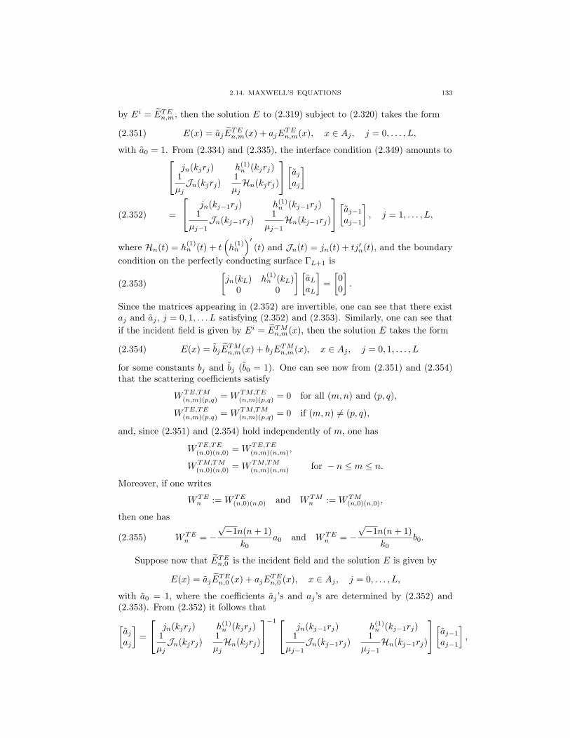
2.14. MAXWELL’S EQUATIONS 133
by Ei = ETEn,m, then the solution E to (2.319) subject to (2.320) takes the form
(2.351) E(x) = ajETEn,m(x) + ajE
TEn,m(x), x ∈ Aj , j = 0, . . . , L,
with a0 = 1. From (2.334) and (2.335), the interface condition (2.349) amounts to
jn(kjrj) h(1)n (kjrj)1
µjJn(kjrj)
1
µjHn(kjrj)
[ajaj
]
=
jn(kj−1rj) h(1)n (kj−1rj)1
µj−1Jn(kj−1rj)
1
µj−1Hn(kj−1rj)
[aj−1
aj−1
], j = 1, . . . , L,(2.352)
where Hn(t) = h(1)n (t) + t
(h(1)n
)′(t) and Jn(t) = jn(t) + tj′n(t), and the boundary
condition on the perfectly conducting surface ΓL+1 is
(2.353)
[jn(kL) h
(1)n (kL)
0 0
] [aLaL
]=
[00
].
Since the matrices appearing in (2.352) are invertible, one can see that there existaj and aj , j = 0, 1, . . . L satisfying (2.352) and (2.353). Similarly, one can see that
if the incident field is given by Ei = ETMn,m(x), then the solution E takes the form
(2.354) E(x) = bjETMn,m(x) + bjE
TMn,m(x), x ∈ Aj , j = 0, 1, . . . , L
for some constants bj and bj (b0 = 1). One can see now from (2.351) and (2.354)that the scattering coefficients satisfy
WTE,TM(n,m)(p,q) =WTM,TE
(n,m)(p,q) = 0 for all (m,n) and (p, q),
WTE,TE(n,m)(p,q) =WTM,TM
(n,m)(p,q) = 0 if (m,n) 6= (p, q),
and, since (2.351) and (2.354) hold independently of m, one has
WTE,TE(n,0)(n,0) =WTE,TE
(n,m)(n,m),
WTM,TM(n,0)(n,0) =WTM,TM
(n,m)(n,m) for − n ≤ m ≤ n.
Moreover, if one writes
WTEn :=WTE
(n,0)(n,0) and WTMn :=WTM
(n,0)(n,0),
then one has
(2.355) WTEn = −
√−1n(n+ 1)
k0a0 and WTE
n = −√−1n(n+ 1)
k0b0.
Suppose now that ETEn,0 is the incident field and the solution E is given by
E(x) = ajETEn,0 (x) + ajE
TEn,0 (x), x ∈ Aj , j = 0, . . . , L,
with a0 = 1, where the coefficients aj ’s and aj ’s are determined by (2.352) and(2.353). From (2.352) it follows that
[ajaj
]=
jn(kjrj) h(1)n (kjrj)1
µjJn(kjrj)
1
µjHn(kjrj)
−1
jn(kj−1rj) h(1)n (kj−1rj)1
µj−1Jn(kj−1rj)
1
µj−1Hn(kj−1rj)
[aj−1
aj−1
],

134 2. LAYER POTENTIALS
for j = 1, . . . , L. Substituting these relations into (2.353) yields
(2.356)
[00
]= PTEn [ε, µ, ω]
[a0a0
],
where
PTEn [ε, µ, ω] :=
[pTEn,1 pTEn,20 0
]= (−
√−1ω)L
L∏
j=1
µ32j ε
12j rj
[jn(kL) h
(1)n (kL)
0 0
]
×L∏
j=1
1
µjHn(kjrj) −h(1)n (kjrj)
− 1
µjJn(kjrj) jn(kjrj)
jn(kj−1rj) h(1)n (kj−1rj)1
µj−1Jn(kj−1rj)
1
µj−1Hn(kj−1rj)
.
(2.357)
Then (2.356) yields
(2.358) WTEn = −
√−1n(n+ 1)
k0a0 = −
√−1n(n+ 1)
k0
pTEn,1pTEn,2
.
Similarly, for WTMn , one looks for another solution E of the form
E(x) = bjETMn,0 (x) + bjE
TMn,0 (x), x ∈ Aj , j = 0, . . . , L,
with b0 = 1. The transmission conditions become1
εjJn(kjrj)
1
εjHn(kjrj)
jn(kjrj) h(1)n (kjrj)
[bjbj
]
=
1
εj−1Jn(kj−1rj)
1
εj−1Hn(kj−1rj)
jn(kj−1rj) h(1)n (kj−1rj)
[bj−1
bj−1
], j = 1, . . . , N + 1,(2.359)
and the boundary condition on the inner most layer, which is perfectly conducting,is
(2.360)
[Jn(kL) Hn(kL)
0 0
] [bLbL
]=
[00
].
From (2.359) and (2.360), one obtains
(2.361)
[00
]= PTMn [ε, µ, ω]
[b0b0
],
where
PTMn [ε, µ, ω] :=
[pTMn,1 pTMn,20 0
]= (iω)L
L∏
j=1
µ12j ε
32j rj
[Jn(kL) Hn(kL)
0 0
]
×L∏
j=1
h(1)n (kjrj) − 1
εjHn(kjrj)
−jn(kjrj)1
εjJn(kjrj)
1
εj−1Jn(kj−1rj)
1
εj−1Hn(kj−1rj)
jn(kj−1rj) h(1)n (kj−1rj)
.
(2.362)

2.14. MAXWELL’S EQUATIONS 135
From the definition of WTMn and (2.361),
(2.363) WTEn = −
√−1n(n+ 1)
k0
b0
b0= −
√−1n(n+ 1)
k0
pTMn,1pTMn,2
.
It is worth emphasizing that pTEn,2 6= 0 and pTMn,2 6= 0. In fact, if pTEn,2 = 0, then(2.356) can be fulfilled with a0 = 0 and a0 = 1. This means that there exists (µ, ε)on R3 \D such that the following problem has a solution:
∇× E =√−1ωµH in R3 \D,
∇×H = −√−1ωεE in R3 \D,
(x× E)∣∣+= 0 on ∂D,
E(x) = ETEn,0 (x) for |x| > 2.
Applying the following Green’s theorem on Ω = x : 1 < |x| < R,∫
Ω
(E ·∆F + curlE · curlF +∇ · E ∇ · F
)dx
=
∫
∂Ω
(ν × E · curlF + ν · E (∇ · F )
)dσ(x)
with F = ETEn,0 (x) and the boundary condition on the perfectly conducting surface
|x| = 1, it follows that∫
|x|=R(ν × E) ·Hdσ(x) =
√−1k0
∫
Ω
(|H|2 − |E|2)dx.
In particular, the left-hand side is real-valued. Hence,∫
|x|=R|H × ν − E|2dσ(x) =
∫
|x|=R
(|H × ν|2 + |E|2 − 2ℜ((ν × E) ·H
)dσ(x)
=
∫
|x|=R
(|H × ν|2 + |E|2
)dσ(x).
From the radiation condition, the left-hand side goes to zero as R → ∞, whichcontradicts the behavior of the Hankel functions. One can show that pTMn,2 6= 0 in asimilar way.
2.14.6.3. Numerical Example. We now demonstrate how to compute the scat-tering coefficients WTE
n and WTMn numerically using Code Scattering Coefficients
for Maxwell’s Equations. For simplicity, we consider only WTEn . Recall that
(2.364) WTEn = −
√−1n(n+ 1)
k0a0,
with the constant a0 being determined by (2.352) and (2.353). From (2.352), weobtain
(2.365)
[a0/aLa0/aL
]= (M−1
1 N1)(M−12 N2) . . . (M
−1L NL)
[aL/aL
1
],
where
Mj =
jn(kjrj) h(1)n (kjrj)1
µjJn(kjrj)
1
µjHn(kjrj)
, Nj =
jn(kj−1rj) h(1)n (kj−1rj)1
µj−1Jn(kj−1rj)
1
µj−1Hn(kj−1rj)
.

136 2. LAYER POTENTIALS
From (2.353), we immediately see that
aLaL
= −h(1)n (kLrL+1)
jn(kLrL+1).
Therefore, we can compute a0/aL and a0/aL. But, since a0 = 1, we can alsocompute a0 and then WTE
n .Now we present a numerical example. We set the parameters for the structure
as follows: the number of layers L is L = 3, the radii of the layers are r1 = 2, r2 =5/3, r3 = 4/3, r4 = 1, and the material parameters are (ε0, µ0) = (1, 1), (ε0, µ0) =(0.5, 0.5), (ε0, µ0) = (2, 2), (ε0, µ0) = (0.5, 0.5). The numerical result for WTE
n andWTMn for n = 1, 2, . . . , 7 is shown in Table 2.8. The decaying behavior of WTE
n andWTMn is clearly shown.
n WTEn WTM
n
1 −0.9991 + 0.9572√−1 −0.7473 + 1.6644
√−1
2 −0.7527 + 0.0960√−1 −0.7650 + 0.0992
√−1
3 −0.1642 + 0.0022√−1 −0.1643 + 0.0023
√−1
4 −0.0191 + 0.0000√−1 −0.0191 + 0.0000
√−1
5 −0.0013 + 0.0000√−1 −0.0013 + 0.0000
√−1
6 −0.0001 + 0.0000√−1 −0.0001 + 0.0000
√−1
7 −0.0000 + 0.0000√−1 −0.0000 + 0.0000
√−1
Table 2.8. Scattering coefficients for a multi-layer spherical shell.
2.14.7. The Helmholtz-Kirchhoff Theorem. Let
Gkm(x) = εm
(Γkm(x)I +
1
k2mD2xΓkm(x)
)(2.366)
be the Dyadic Green (matrix valued) function for the full Maxwell equations. Thefollowing Helmholtz-Kirchhoff identity holds.
Proposition 2.120. Let ∂BR be the sphere of radius R and center 0. We have(2.367)∫
∂BR
(∂Gkm
∂ν(x−y)Gkm(z−y)−Gkm(x−y)∂Gkm
∂ν(z−y)
)dσ(y) = 2
√−1ℑGkm(x−z) ,
which yields
(2.368) limR→+∞
∫
∂BR
Gkm(x− y)Gkm(z − y) dσ(y) = − 1
kmℑGkm(x− z) ,
by using the Silver-Muller radiation condition.
2.14.8. The Optical Theorem. The optical cross-section theorem for thescattering of electromagnetic waves can be stated as follows [268].
Proposition 2.121. Assume that the incident fields are plane waves given by
Ei(x) = ce√−1kmd·x,
Hi(x) =
√εmµm
d× ce√−1kmd·x,

2.14. MAXWELL’S EQUATIONS 137
where c ∈ R3 and d ∈ S are such that c · d = 0. Then, the extinction cross-sectionQext, defined by
Qext := − 1
|c|2√µmεm
ℜ[ ∫
∂D
(Ei × (H −Hi) + (E − Ei)×Hi
)· ν dσ,
satisfies
Qext =4π
kmℑ[c ·A∞(c, d; d)
|c|2],
where the scattering amplitude A∞(c, d; x) is defined by (2.345) with αll′ and βll′
are given by (2.346).
Analogously to the scalar case, the extinction cross-section Qext is defined asthe ratio of the sum of the mean powers absorbed and scattered by D to the meanintensity power flow in the incident field. The latter quantity is given by
−1
2ℜ[(Ei ×Hi) · d
]
which reduces to1
2
√εmµm
|c|2.
2.14.9. Electromagnetic Scattering by Small Particles. We consider thescattering problem of a time-harmonic electromagnetic wave incident on a particleD. The homogeneous medium is characterized by electric permittivity εm andmagnetic permeability µm, while D is characterized by electric permittivity εc andmagnetic permeability µc. We assume that εm, εc, µm, and µc are positive constantsand define
km = ω√εmµm, kc = ω
√εcµc,
and
εD = εmχ(R3 \D) + εcχ(D), µD = εmχ(R
3 \D) + εcχ(D).
For a given incident plane wave (Ei, Hi), solution to the Maxwell equationsin free space (2.318), the scattering problem can be modeled by the system ofequations (2.319) subject to the Silver-Muller radiation condition (2.320).
Let D = z + δB where B contains the origin and |B| = O(1). The followingresult follows from [70, 80, 82]. It gives the leading-order term in the asymptoticexpansion of the scattered electric field Es far-away from the particle.
Theorem 2.122. For D = z+δB ⋐ R3 of class C1,α for α > 0 and K ⋐ R3\D,the following far-field expansion holds uniformly in K(2.369)
Es(x) = −√−1ωµmεm
∇×Gkm(x− z)M(λµ, D)Hi(z)− ω2µmGkm(x− z)M(λε, D)Ei(z)
+O(δ4),
where Gkm(x−z) is the Dyadic Green (matrix valued) function for the full Maxwellequations defined by (2.366) and M(λµ, D) and M(λε, D) are the polarization ten-sors associated with D and the contrasts λµ and λε given by (2.72) with k = µm/µcand k = εc/εm, respectively.

138 2. LAYER POTENTIALS
2.15. Integral Representation of Solutions to the Lame System
Let Ω be a bounded domain in Rd with a connected Lipschitz boundary. Letλ and µ be the Lame constants for Ω satisfying the strong convexity condition
(2.370) µ > 0 and dλ+ 2µ > 0.
The corresponding Lame system is given by
Lλ,µu = µu+ (λ+ µ)∇∇ · u,and the conormal derivative ∂u/∂ν is defined by
(2.371)∂u
∂ν= λ(∇ · u)N + µ(∇u+∇ut)N,
where the superscript t denotes the transpose and N is the unit normal to theboundary ∂Ω. We introduce the symmetric gradient as
(2.372) ∇su :=1
2(∇u+∇ut)
and define the elasticity tensor C = (Cijkl)di,j,k,l=1 by
(2.373) Cijkl = λδijδkl + µ(δikδjl + δilδjk).
With this notation, we have
Lλ,µu = ∇ · C∇su,
and∂u
∂ν= (C∇su)N.
2.15.1. Fundamental Solutions. In the three-dimensional case, the Kupradzematrix Γω = (Γωij)
3i,j=1 of the fundamental solution to the operator Lλ,µ + ω2 is
given by
Γωij(x) = − δij4πµ|x|e
√−1ω|x|cs +
1
4πω2∂i∂j
e
√−1ω|x|cp − e
√−1ω|x|cs
|x| ,
where ∂j denotes ∂/∂xj and
cs =õ, cp =
√λ+ 2µ.
See [309, Chapter 2]. One can easily show that Γωij has the series representation:
Γωij(x) = − 1
4π
+∞∑
n=0
√−1
n
(n+ 2)n!
(n+ 1
cn+2s
+1
cn+2p
)ωnδij |x|n−1(2.374)
+1
4π
+∞∑
n=0
√−1
n(n− 1)
(n+ 2)n!
( 1
cn+2s
− 1
cn+2p
)ωn|x|n−3xixj .
If ω = 0, then Γ0 is the Kelvin matrix of the fundamental solution to the Lamesystem; i.e.,
(2.375) Γ0ij(x) = − γ1
4π
δij|x| −
γ24π
xixj|x|3 ,
where
(2.376) γ1 =1
2
(1
µ+
1
2µ+ λ
)and γ2 =
1
2
(1
µ− 1
2µ+ λ
).

2.15. INTEGRAL REPRESENTATION OF SOLUTIONS TO THE LAME SYSTEM 139
In the two-dimensional case, the fundamental solution Γω = (Γωij)2i,j=1 to the
operator Lλ,µ + ω2, ω 6= 0, is given by(2.377)
Γωij(x) = −√−1
4µδijH
(1)0
(ω|x|cs
)+
√−1
4ω2∂i∂j
(H
(1)0
(ω|x|cp
)−H
(1)0
(ω|x|cs
)).
See [6] and [309, Chapter 2]. For ω = 0, we set Γ0 to be the Kelvin matrix offundamental solutions to the Lame system; i.e.,
(2.378) Γ0ij(x) =
γ12πδij ln |x| −
γ22π
xixj|x|2 .
2.15.2. Single- and Double-Layer Potentials. Analogously to the Laplaceoperator, the single- and double-layer potentials for the operator Lλ,µ + ω2 aredefined by
SωΩ [ϕ](x) =∫
∂Ω
Γω(x− y)ϕ(y) dσ(y), x ∈ Rd,(2.379)
DωΩ[ϕ](x) =
∫
∂Ω
∂
∂ν(y)Γω(x− y)ϕ(y) dσ(y), x ∈ Rd \ ∂Ω,(2.380)
for ϕ ∈ L2(∂Ω)d. Here, the conormal derivative of Γω is defined by
(2.381)∂
∂ν(y)Γω(x− y)b =
∂
∂ν(y)
(Γω(x− y)b
)
for any constant vector b.The following formulas give the jump relations obeyed by the double-layer
potential and by the conormal derivative of the single-layer potential:
∂(SωΩ [ϕ])∂ν
∣∣∣±(x) =
(± 1
2I + (KωΩ)∗
)[ϕ](x) a.e. x ∈ ∂Ω,(2.382)
(DωΩ[ϕ])
∣∣∣±(x) =
(∓ 1
2I +KωΩ
)[ϕ](x) a.e. x ∈ ∂Ω,(2.383)
where KωΩ is the operator defined by
KωΩ[ϕ](x) = p.v.
∫
∂Ω
∂Γω(x− y)
∂ν(y)ϕ(y) dσ(y)(2.384)
and (KωΩ)∗ is the L2-adjoint of K−ωΩ ; that is,
(KωΩ)∗[ϕ](x) = p.v.
∫
∂Ω
∂Γω(x− y)
∂ν(x)ϕ(y) dσ(y).
See [309, 190].Let Ψ be the vector space of all linear solutions to the equation Lλ,µu = 0 and
∂u/∂ν = 0 on ∂Ω, or alternatively,
(2.385) Ψ =
ψ : ∂iψj + ∂jψi = 0, 1 ≤ i, j ≤ d
.
Define a subspace of L2(∂Ω)d by
L2Ψ(∂Ω) =
f ∈ L2(∂Ω)d :
∫
∂Ω
f · ψ dσ = 0 for all ψ ∈ Ψ
.

140 2. LAYER POTENTIALS
In particular, since Ψ contains constant functions, we get∫
∂Ω
f dσ = 0
for any f ∈ L2Ψ(∂Ω). We also know that if u is smooth and satisfies Lλ,µu = 0 in
Ω, then ∂u/∂ν∣∣∂Ω
∈ L2Ψ(∂Ω).
We recall Green’s formulas for the Lame system, which can be obtained byintegration by parts. The first formula is∫
∂Ω
u · ∂v∂ν
dσ =
∫
Ω
u · Lλ,µv +E(u,v),(2.386)
where u ∈ H1(Ω)d, v ∈ H3/2(Ω)d, and
E(u,v) =
∫
Ω
λ(∇ · u)(∇ · v) + µ
2(∇u+∇ut) · (∇v +∇v
t).(2.387)
Formula (2.386) yields Green’s second formula∫
∂Ω
(u · ∂v
∂ν− v · ∂u
∂ν
)=
∫
Ω
(u · Lλ,µv − v · Lλ,µu
),(2.388)
where u, v ∈ H3/2(Ω)d.Formula (2.388) shows that if u ∈ H3/2(Ω)d satisfies Lλ,µu = 0 in Ω, then
∂u/∂ν∣∣∂Ω
∈ L2Ψ(∂Ω).
2.15.3. Helmholtz Decompositions and Radiation Conditions. Let usformulate the radiation conditions for the elastic waves when ℑω ≥ 0 and ω 6= 0.
Any smooth solution u to the constant-coefficient equation (Lλ,µ + ω2)u = 0can be decomposed as follows [309, Theorem 2.5]:
(2.389) u = up + us,
where up and us are given by
up = (κ2s − κ2p)−1(+ κ2s)u,
us = (κ2p − κ2s)−1(+ κ2p)u,
with
(2.390) κs =ω
cs=
ω√µ
and κp =ω
cp=
ω√λ+ 2µ
.
Then us and up satisfy the equations
(2.391)
(+ κ2s)us = 0, ∇× us = 0,
(+ κ2p)up = 0, ∇ · up = 0.
We impose on us and up the radiation condition (2.153) for solutions of theHelmholtz equation by requiring that
(2.392)
∂rus(x)−
√−1κsus(x) = o(r−1),
∂rup(x)−√−1κpup(x) = o(r−1),
as r = |x| → +∞.
We say that u satisfies the Sommerfeld-Kupradze radiation condition if it can bedecomposed in the form (2.389) with us and up satisfying (2.391) and (2.392). By astraightforward calculation, one can see that the single- and double-layer potentialssatisfy the radiation condition. We refer to [5, 309] for details.
We recall the following uniqueness results for the exterior problem [309].

2.15. INTEGRAL REPRESENTATION OF SOLUTIONS TO THE LAME SYSTEM 141
Lemma 2.123. Let u be a solution to (Lλ,µ+ω2)u = 0 in Rd \Ω satisfying theradiation condition. If either u = 0 or ∂u/∂ν = 0 on ∂Ω, then u is identically zeroin Rd \ Ω.
In dimension d, the Kupradze matrix Γω can be decomposed into shear andpressure components [7]:
(2.393) Γω(x) = Γωs (x) + Γωp (x), x ∈ Rd, x 6= 0,
where
(2.394) Γωp (x) = − 1
µκ2sDΓκp(x) and Γωs (x) =
1
µκ2s(κ2sI+D)Γκs(x).
Here, the tensor D is defined by
(2.395) D = (∂2ij)di,j=1,
and the functions Γκpand Γκs
are defined by (2.147).
2.15.4. Transmission Problem. Let λ, µ be another pair of Lame parame-ters such that
(2.396) (λ− λ)(µ− µ) ≥ 0, (λ− λ)2 + (µ− µ)2 6= 0.
Later in this book, we will consider the following transmission problem:
(2.397)
Lλ,µu+ ω2u = 0 in Ω \D,Lλ,µu+ ω2u = 0 in D,
∂u
∂ν= g on ∂Ω,
u∣∣+− u
∣∣− = 0 on ∂D,
∂u
∂ν
∣∣+− ∂u
∂ν
∣∣− = 0 on ∂D.
Let SωD denote the single-layer potential defined by (2.379) with λ, µ replaced
by λ, µ. We also denote by ∂u/∂ν the conormal derivative associated with λ, µ.We now have the following solvability result which can be viewed as a compactperturbation result of the case ω = 0.
Theorem 2.124. Suppose that (λ − λ)(µ − µ) ≥ 0 and 0 < λ, µ < +∞.Suppose that ℑω ≥ 0 and ω2 is not a Dirichlet eigenvalue for −Lλ,µ on D. For anygiven (F,G) ∈ H1(∂D)d × L2(∂D)d, there exists a unique pair (f ,g) ∈ L2(∂D)d ×L2(∂D)d such that
SωD[f ]|− − SωD[g]|+ = F,
∂
∂νSωD[f ]
∣∣∣−− ∂
∂νSωD[g]
∣∣∣+= G.
If ω = 0 and G ∈ L2Ψ(∂D), then g ∈ L2
Ψ(∂D). Moreover, if F ∈ Ψ and G = 0,then g = 0.
Proof. For ω = 0, the theorem is proved in [211]. Here, we only consider thecase ω 6= 0, which can be treated as a compact perturbation of the case ω = 0. In

142 2. LAYER POTENTIALS
fact, let us define the operators T, T0 : L2(∂D)d×L2(∂D)d → H1(∂D)d×L2(∂D)d
by
T (f ,g) :=
(SωD[f ]|− − SωD[g]|+,
∂
∂νSωD[f ]
∣∣∣−− ∂
∂νSωD[g]
∣∣∣+
)
and
T0(f ,g) :=
(S0D[f ]|− − S0
D[g]|+,∂
∂νS0D[f ]
∣∣∣−− ∂
∂νS0D[g]
∣∣∣+
).
It is easily checked that T − T0 is a compact operator. Since we know that T0is invertible, by the Fredholm alternative, it is enough to show that T is injective.Suppose that T (f ,g) = 0. Then the function u given by
u(x) :=
SωD[g](x), x ∈ Rd \D,SωD[f ](x), x ∈ D,
is a solution to the transmission problem
Lλ,µu+ ω2u = 0 in Rd \D,Lλ,µu+ ω2u = 0 in D,
u∣∣+− u
∣∣− = 0 on ∂D,
∂u
∂ν
∣∣+− ∂u
∂ν
∣∣− = 0 on ∂D,
satisfying the radiation condition. By the uniqueness of a solution to this trans-mission problem, see for instance [309, Chapter 3], we have u = 0. From theassumption on ω, we conclude that f = g = 0. This completes the proof.
For transmission problems such as (2.397), the following representation formulaholds.
Theorem 2.125. Let ℑω ≥ 0. Suppose that ω2 is not a Dirichlet eigenvaluefor −Lλ,µ on D. Let u be a solution of (2.397) and f := u|∂Ω. Define
(2.398) H(x) := DωΩ[f ](x)− SωΩ [g](x), x ∈ Rd \ ∂Ω.
Then u can be represented as
(2.399) u(x) =
H(x) + SωD[ψ](x), x ∈ Ω \D,SωD[φ](x), x ∈ D,
where the pair (φ, ψ) ∈ L2(∂D)d × L2(∂D)d is the unique solution of
(2.400)
SωD[φ]− SωD[ψ] = H|∂D,∂
∂νSωD[φ]−
∂
∂νSωD[ψ] =
∂H
∂ν
∣∣∣∂D.
Moreover, we have
(2.401) H(x) + SωD[ψ](x) = 0, x ∈ Rd \ Ω.

2.15. INTEGRAL REPRESENTATION OF SOLUTIONS TO THE LAME SYSTEM 143
Proof. We consider the following two-phase transmission problem:
(2.402)
Lλ,µv + ω2v = 0 in (Ω \D)⋃(Rd \ Ω),
Lλ,µv + ω2v = 0 in D,
v∣∣− − v
∣∣+= f ,
∂v
∂ν
∣∣− − ∂v
∂ν
∣∣+= g on ∂Ω,
v∣∣− − v
∣∣+= 0,
∂v
∂ν
∣∣− − ∂v
∂ν
∣∣+= 0 on ∂D,
with the radiation condition. This problem has a unique solution. See [309, Chap-ter 3]. It is easily checked that both v and v defined by
v(x) =
u(x), x ∈ Ω,
0, x ∈ Rd \ Ω,and
v(x) =
H(x) + SωD[ψ](x), x ∈ Rd \
(D ∪ ∂Ω
),
SωD[φ](x), x ∈ D,
are solutions to (2.402). Hence v = v, which concludes the proof of the theorem.
2.15.5. Eigenvalue Characterization. Let κ be an eigenvalue of −Lλ,µ inΩ with the Neumann condition on ∂Ω and let u denote an eigenfunction associatedwith κ; i.e.,
(2.403)
Lλ,µu+ κu = 0 in Ω,
∂u
∂ν= 0 on ∂Ω.
We note that since−Lλ,µ is elliptic, it has discrete eigenvalues of finite multiplicities.The following proposition from [309, Chapter 7] is of importance to us.
Proposition 2.126 (Eigenvalue characterization). The necessary and suffi-cient condition for (2.403) to have a nontrivial solution is that κ is nonnegativeand
√κ coincides with one of the characteristic values of (1/2) I − KωΩ. If κ = ω2
0
is an eigenvalue of (2.403) with multiplicity m, then((1/2) I − Kω0
Ω
)[φ] = 0 has
m linearly independent solutions. Moreover, for every eigenvalue κ > 0,√κ is a
simple pole of the operator-valued function ω 7→ ((1/2) I −KωΩ)−1.
2.15.6. Neumann Function. Let 0 ≤ κ1 ≤ κ2 ≤ . . . be the eigenvalues of−Lλ,µ in Ω with the Neumann condition on ∂Ω. For ω /∈ √κjj≥1, let Nω
Ω(x, z)
be the Neumann function for Lλ,µ + ω2 in Ω corresponding to a Dirac mass at z.That is, Nω
Ω is the solution to
(2.404)
(Lλ,µ + ω2)Nω
Ω(x, z) = −δz(x)I, x ∈ Ω,
∂NωΩ
∂ν(x, z) = 0, x ∈ ∂Ω.
Then the following relation, which can be proved similarly to (2.183), holds (see[45]):
(2.405)(− 1
2I+KωΩ
)[Nω
Ω(·, z)](x) = Γω(x, z), x ∈ ∂Ω, z ∈ Ω.
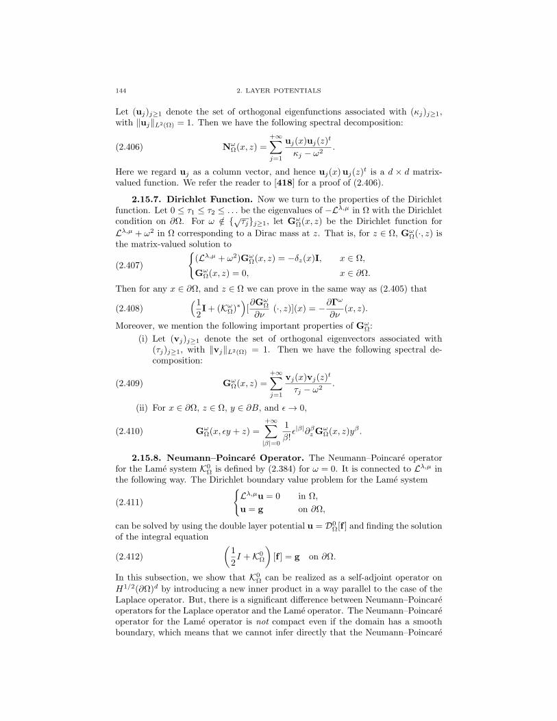
144 2. LAYER POTENTIALS
Let (uj)j≥1 denote the set of orthogonal eigenfunctions associated with (κj)j≥1,with ‖uj‖L2(Ω) = 1. Then we have the following spectral decomposition:
(2.406) NωΩ(x, z) =
+∞∑
j=1
uj(x)uj(z)t
κj − ω2.
Here we regard uj as a column vector, and hence uj(x)uj(z)t is a d × d matrix-
valued function. We refer the reader to [418] for a proof of (2.406).
2.15.7. Dirichlet Function. Now we turn to the properties of the Dirichletfunction. Let 0 ≤ τ1 ≤ τ2 ≤ . . . be the eigenvalues of −Lλ,µ in Ω with the Dirichletcondition on ∂Ω. For ω /∈ √τjj≥1, let Gω
Ω(x, z) be the Dirichlet function for
Lλ,µ + ω2 in Ω corresponding to a Dirac mass at z. That is, for z ∈ Ω, GωΩ(·, z) is
the matrix-valued solution to
(2.407)
(Lλ,µ + ω2)Gω
Ω(x, z) = −δz(x)I, x ∈ Ω,
GωΩ(x, z) = 0, x ∈ ∂Ω.
Then for any x ∈ ∂Ω, and z ∈ Ω we can prove in the same way as (2.405) that
(2.408)(12I+ (KωΩ)∗
)[∂Gω
Ω
∂ν(·, z)](x) = −∂Γ
ω
∂ν(x, z).
Moreover, we mention the following important properties of GωΩ:
(i) Let (vj)j≥1 denote the set of orthogonal eigenvectors associated with(τj)j≥1, with ‖vj‖L2(Ω) = 1. Then we have the following spectral de-composition:
(2.409) GωΩ(x, z) =
+∞∑
j=1
vj(x)vj(z)t
τj − ω2.
(ii) For x ∈ ∂Ω, z ∈ Ω, y ∈ ∂B, and ǫ→ 0,
(2.410) GωΩ(x, ǫy + z) =
+∞∑
|β|=0
1
β!ǫ|β|∂βzG
ωΩ(x, z)y
β .
2.15.8. Neumann–Poincare Operator. The Neumann–Poincare operatorfor the Lame system K0
Ω is defined by (2.384) for ω = 0. It is connected to Lλ,µ inthe following way. The Dirichlet boundary value problem for the Lame system
(2.411)
Lλ,µu = 0 in Ω,
u = g on ∂Ω,
can be solved by using the double layer potential u = D0Ω[f ] and finding the solution
of the integral equation
(2.412)
(1
2I +K0
Ω
)[f ] = g on ∂Ω.
In this subsection, we show that K0Ω can be realized as a self-adjoint operator on
H1/2(∂Ω)d by introducing a new inner product in a way parallel to the case of theLaplace operator. But, there is a significant difference between Neumann–Poincareoperators for the Laplace operator and the Lame operator. The Neumann–Poincareoperator for the Lame operator is not compact even if the domain has a smoothboundary, which means that we cannot infer directly that the Neumann–Poincare
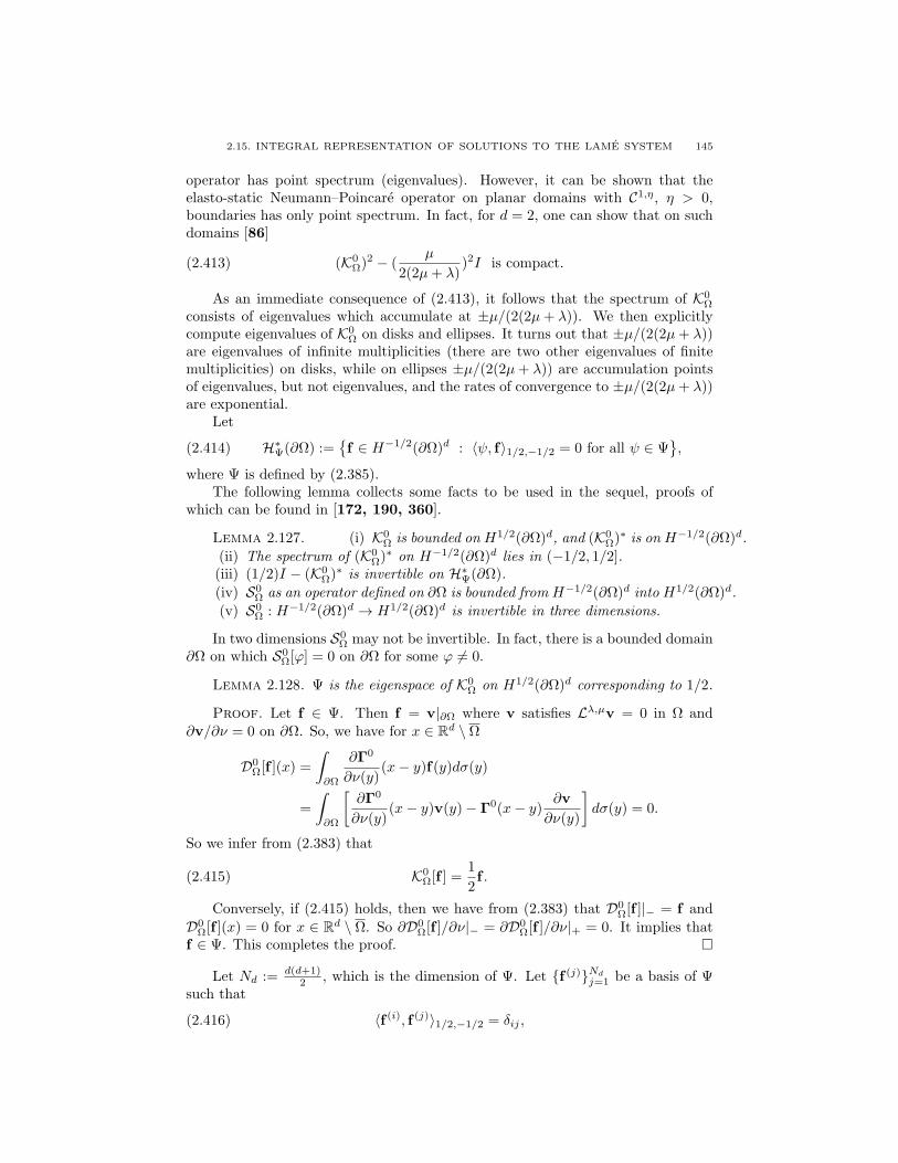
2.15. INTEGRAL REPRESENTATION OF SOLUTIONS TO THE LAME SYSTEM 145
operator has point spectrum (eigenvalues). However, it can be shown that theelasto-static Neumann–Poincare operator on planar domains with C1,η, η > 0,boundaries has only point spectrum. In fact, for d = 2, one can show that on suchdomains [86]
(2.413) (K0Ω)
2 − (µ
2(2µ+ λ))2I is compact.
As an immediate consequence of (2.413), it follows that the spectrum of K0Ω
consists of eigenvalues which accumulate at ±µ/(2(2µ+ λ)). We then explicitlycompute eigenvalues of K0
Ω on disks and ellipses. It turns out that ±µ/(2(2µ+ λ))are eigenvalues of infinite multiplicities (there are two other eigenvalues of finitemultiplicities) on disks, while on ellipses ±µ/(2(2µ+ λ)) are accumulation pointsof eigenvalues, but not eigenvalues, and the rates of convergence to ±µ/(2(2µ+ λ))are exponential.
Let
(2.414) H∗Ψ(∂Ω) :=
f ∈ H−1/2(∂Ω)d : 〈ψ, f〉1/2,−1/2 = 0 for all ψ ∈ Ψ
,
where Ψ is defined by (2.385).The following lemma collects some facts to be used in the sequel, proofs of
which can be found in [172, 190, 360].
Lemma 2.127. (i) K0Ω is bounded on H1/2(∂Ω)d, and (K0
Ω)∗ is on H−1/2(∂Ω)d.
(ii) The spectrum of (K0Ω)
∗ on H−1/2(∂Ω)d lies in (−1/2, 1/2].(iii) (1/2)I − (K0
Ω)∗ is invertible on H∗
Ψ(∂Ω).
(iv) S0Ω as an operator defined on ∂Ω is bounded from H−1/2(∂Ω)d into H1/2(∂Ω)d.
(v) S0Ω : H−1/2(∂Ω)d → H1/2(∂Ω)d is invertible in three dimensions.
In two dimensions S0Ω may not be invertible. In fact, there is a bounded domain
∂Ω on which S0Ω[ϕ] = 0 on ∂Ω for some ϕ 6= 0.
Lemma 2.128. Ψ is the eigenspace of K0Ω on H1/2(∂Ω)d corresponding to 1/2.
Proof. Let f ∈ Ψ. Then f = v|∂Ω where v satisfies Lλ,µv = 0 in Ω and∂v/∂ν = 0 on ∂Ω. So, we have for x ∈ Rd \ Ω
D0Ω[f ](x) =
∫
∂Ω
∂Γ0
∂ν(y)(x− y)f(y)dσ(y)
=
∫
∂Ω
[∂Γ0
∂ν(y)(x− y)v(y)− Γ0(x− y)
∂v
∂ν(y)
]dσ(y) = 0.
So we infer from (2.383) that
(2.415) K0Ω[f ] =
1
2f .
Conversely, if (2.415) holds, then we have from (2.383) that D0Ω[f ]|− = f and
D0Ω[f ](x) = 0 for x ∈ Rd \ Ω. So ∂D0
Ω[f ]/∂ν|− = ∂D0Ω[f ]/∂ν|+ = 0. It implies that
f ∈ Ψ. This completes the proof.
Let Nd := d(d+1)2 , which is the dimension of Ψ. Let f (j)Nd
j=1 be a basis of Ψsuch that
(2.416) 〈f (i), f (j)〉1/2,−1/2 = δij ,
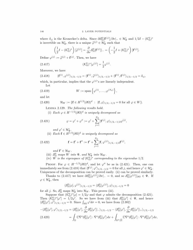
146 2. LAYER POTENTIALS
where δij is the Kronecker’s delta. Since ∂S0Ω[f
(j)]/∂ν|− ∈ H∗Ψ and 1/2I − (K0
Ω)∗
is invertible on H∗Ψ, there is a unique ϕ(j) ∈ H∗
Ψ such that(1
2I − (K0
Ω)∗)[ϕ(j)] =
∂
∂νS0Ω[f
(j)]|− =
(−1
2I + (K0
Ω)∗)[f (j)].
Define ϕ(j) := ϕ(j) + f (j). Then, we have
(2.417) (K0Ω)
∗[ϕ(j)] =1
2ϕ(j).
Moreover, we have
(2.418) 〈f (i), ϕ(j)〉1/2,−1/2 = 〈f (i), ϕ(j)〉1/2,−1/2 + 〈f (i), f (j)〉1/2,−1/2 = δij ,
which, in particular, implies that the ϕ(j)’s are linearly independent.Let
(2.419) W := spanϕ(1), . . . , ϕ(Nd)
,
and let
(2.420) HW := f ∈ H1/2(∂Ω)d : 〈f , ϕ〉1/2,−1/2 = 0 for all ϕ ∈W.Lemma 2.129. The following results hold.
(i) Each ϕ ∈ H−1/2(∂Ω)d is uniquely decomposed as
(2.421) ϕ = ϕ′ + ϕ′′ := ϕ′ +Nd∑
j=1
〈f (j), ϕ〉1/2,−1/2ϕ(j),
and ϕ′ ∈ H∗Ψ.
(ii) Each f ∈ H1/2(∂Ω)d is uniquely decomposed as
(2.422) f = f ′ + f ′′ := f ′ +Nd∑
j=1
〈f , ϕ(j)〉1/2,−1/2f(j),
and f ′ ∈ HW .(iii) S0
Ω maps W into Ψ, and H∗Ψ into HW .
(iv) W is the eigenspace of (K0Ω)
∗ corresponding to the eigenvalue 1/2.
Proof. For ϕ ∈ H−1/2(∂Ω)d, and let ϕ′′ be as in (2.421). Then, one canimmediately see from (2.418) that 〈f (j), ϕ′〉1/2,−1/2 = 0 for all j, and hence ϕ′ ∈ H∗
Ψ.Uniqueness of the decomposition can be proved easily. (ii) can be proved similarly.
Thanks to (2.417) we have ∂S0Ω[ϕ
(j)]/∂ν|− = 0, and so S0Ω[ϕ
(j)]|∂Ω ∈ Ψ. Ifϕ ∈ H∗
Ψ, then
〈S0Ω[ϕ], ϕ
(j)〉1/2,−1/2 = 〈S0Ω[ϕ
(j)], ϕ〉1/2,−1/2 = 0
for all j. So, S0Ω maps H∗
Ψ into HW . This proves (iii).Suppose that (K0
Ω)∗[ϕ] = 1/2ϕ and that ϕ admits the decomposition (2.421).
Then (K0Ω)
∗[ϕ′] = 1/2ϕ′. So we have from (iii) that S0Ω[ϕ
′] ∈ Ψ, and hence〈S0
Ω[ϕ′], ϕ′〉1/2,−1/2 = 0. Since
∫∂Ωϕ′dσ = 0, we have from (2.382)
−〈S0Ω[ϕ
′], ϕ′〉1/2,−1/2 = 〈S0Ω[ϕ
′],∂
∂νS0Ω[ϕ
′]|−〉1/2,−1/2 − 〈S0Ω[ϕ
′],∂
∂νS0Ω[ϕ
′]|+〉1/2,−1/2
=
∫
Ω
C∇sS0Ω[ϕ
′] : ∇sS0Ω[ϕ
′] dx+
∫
Rd\ΩC∇sS0
Ω[ϕ′] : ∇sS0
Ω[ϕ′] dx,(2.423)

2.15. INTEGRAL REPRESENTATION OF SOLUTIONS TO THE LAME SYSTEM 147
where C defined by (2.373) is the elasticity tensor associated with (λ, µ) and A :
B =∑di,j=1 aijbij for matrices A = (aij) and B = (bij). So S0
Ω[ϕ′] ∈ Ψ. Thus we
have ϕ′ = ∂∂νS0
Ω[ϕ′]|+ − ∂
∂νS0Ω[ϕ
′]|− = 0, and hence ϕ ∈ W . Thus (iv) is proved.This completes the proof.
Remark 2.130. In three dimensions, it was recently proved in [89] that theNeumann–Poincare operator defined on a smooth bounded domain is polynomiallycompact. Its spectrum consists of three non-empty sequences of eigenvalues accu-mulating to a certain numbers determined by the Lame parameters.
2.15.9. Symmetrization of the Neumann–Poincare Operator. In thissubsection we introduce a new inner product on H−1/2(∂Ω)d (and H1/2(∂Ω)d)which makes the Neumann–Poincare operator operator (K0
Ω)∗ self-adjoint.
In three dimensions, S0Ω[ϕ](x) = O(|x|−1) as |x| → ∞. Using this fact, one can
show that −S0Ω is positive-definite. In fact, similarly to (2.423) we obtain
(2.424)
−〈S0Ω[ϕ], ϕ〉1/2,−1/2 =
∫
Ω
C∇sS0Ω[ϕ] : ∇sS0
Ω[ϕ] dx+
∫
R3\ΩC∇sS0
Ω[ϕ] : ∇sS0Ω[ϕ] dx ≥ 0.
If 〈S0Ω[ϕ],ϕ〉1/2,−1/2 = 0, then S0
Ω[ϕ] belongs to Ψ. Thus we haveϕ = ∂S0Ω[ϕ]/∂ν|+−
∂S0Ω[ϕ]/∂ν|− = 0. So, if we define
(2.425) 〈ϕ,ψ〉H∗ := −〈S0Ω[ϕ],ϕ〉1/2,−1/2,
it is an inner product on H−1/2(∂Ω)3.In two dimensions, the same argument shows that −S0
Ω is positive-definite onH∗
Ψ. In fact, if ϕ ∈ H∗Ψ, then S0
Ω[ϕ](x) = O(|x|−1) as |x| → ∞, and hence we canapply the same argument as in three dimensions. However, −S0
Ω may fail to bepositive on W : if Ω is the disk of radius r (centered at 0), then we have
(2.426) S0Ω[c](x) =
[α1r ln r −
α2r
2
]c for x ∈ Ω.
for any constant vector c = (c1, c2)t. It shows that −S0
Ω can be positive or negativedepending on r. To see (2.426), we note that
S0Ω[c]i(x) =
α1ci2π
∫
∂Ω
ln |x− y|dσ(y)− α2
2π
2∑
j=1
cj
∫
∂Ω
(x− y)i(x− y)j|x− y|2 dσ(y)
= α1ciS[1](x)− α2
(xic · ∇S[1](x)− c · ∇S[yi](x)
),
where S is the electro-static single layer potential, namely,
(2.427) S[f ](x) = 1
2π
∫
∂Ω
ln |x− y|f(y) dσ(y).
It is known (see [31]) that S[1](x) = r ln r and S[yi](x) = − rxi
2 for x ∈ Ω. So wehave (2.426).
We introduce a variance of S0Ω in two dimensions. For ϕ ∈ H−1/2(∂Ω)2, define
using the decomposition (2.421)
(2.428) S0Ω[ϕ] := S0
Ω[ϕ′] +
3∑
j=1
〈f (j),ϕ〉1/2,−1/2f(j).

148 2. LAYER POTENTIALS
We emphasize that S0Ω[ϕ] = S0
Ω[ϕ] for all ϕ ∈ H∗Ψ and S0
Ω[ϕ(j)] = f (j), j = 1, 2, 3.
In view of (2.418) and Lemma 2.129 (iii), we have
(2.429) − 〈S0Ω[ϕ],ϕ〉1/2,−1/2 = −〈S0
Ω[ϕ′],ϕ′〉1/2,−1/2 +
3∑
j=1
|〈f (j),ϕ〉1/2,−1/2|2.
So, −S0Ω is positive-definite on H−1/2(∂Ω)2. In fact, since −〈S0
Ω[ϕ′],ϕ′〉1/2,−1/2 ≥
0, we have−〈S0Ω[ϕ],ϕ〉1/2,−1/2 ≥ 0. If−〈S0
Ω[ϕ],ϕ〉1/2,−1/2 = 0, then−〈S0Ω[ϕ
′],ϕ′〉1/2,−1/2 =
0 and∑3j=1 |〈f (j),ϕ〉1/2,−1/2|2 = 0. So, ϕ′ = 0 and 〈f (j),ϕ〉1/2,−1/2 = 0 for all j,
and hence ϕ = 0.
Let us also denote S0Ω in three dimensions by S0
Ω for convenience. Define
(2.430) 〈ϕ,ψ〉H∗ := −〈S0Ω[ψ],ϕ〉1/2,−1/2, ϕ,ψ ∈ H−1/2(∂Ω)d.
Proposition 2.131. 〈·, ·〉H∗ is an inner product on H−1/2(∂Ω)d. The norminduced by 〈·, ·〉H∗ , denoted by ‖ · ‖∗, is equivalent to the H−1/2-norm.
Proof. Positive-definiteness of−S0Ω implies that S0
Ω : H−1/2(∂Ω)d → H1/2(∂Ω)d
is bijective. So, we have
‖ϕ‖−1/2 ≈ ‖S0Ω[ϕ]‖1/2.
Here and throughout this chapter A . B means that there is a constant C suchthat A ≤ CB, and A ≈ B means A . B and B . A. It then follows from thedefinition (2.430) that
|〈ϕ,ϕ〉H∗ | ≤ ‖ϕ‖H−1/2‖S0Ω[ϕ]‖1/2 . ‖ϕ‖2H−1/2 .
We have from the Cauchy Schwarz inequality
|〈S0Ω[ψ],ϕ〉1/2,−1/2| = |〈ϕ,ψ〉H∗ | ≤ ‖ϕ‖H∗‖ψ‖H∗ . ‖ϕ‖H∗‖S0
Ω[ψ]‖H1/2 .
So we have
‖ϕ‖−1/2 = supψ 6=0
|〈S0Ω[ψ],ϕ〉1/2,−1/2|‖S0
Ω[ψ]‖1/2. ‖ϕ‖∗.
This completes the proof.
We may define a new inner product on H1/2(∂Ω)d by(2.431)
〈f ,g〉H := 〈(S0Ω)
−1[f ], (S0Ω)
−1[g]〉H∗ = −〈g, (S0Ω)
−1[f ]〉1/2,−1/2, f ,g ∈ H1/2(∂Ω)d.
Proposition 2.132. 〈·, ·〉H is an inner product on H1/2(∂Ω)d. The norm
induced by 〈·, ·〉, denoted by ‖ · ‖H, is equivalent to ‖ · ‖H1/2 . Moreover, S0Ω is
an isometry between H−1/2(∂Ω)d and H1/2(∂Ω)d.
As for the Laplace operator, the Neumann–Poincare operator (K0Ω)
∗ associated
to the Lame system can be realized as a self-adjoint operator on H−1/2(∂Ω)d usingPlemelj’s symmetrization principle which states that
(2.432) S0Ω(K0
Ω)∗ = K0
ΩS0Ω.
This relation is a consequence of the Green’s formula. In fact, if Lλ,µu = 0 in Ω,then we have for x ∈ Rd \ Ω
S0Ω
[∂u
∂ν|−](x)−D0
Ω[u|−](x) = 0.

2.15. INTEGRAL REPRESENTATION OF SOLUTIONS TO THE LAME SYSTEM 149
Substituting u(x) = S0Ω[ϕ](x) for some ϕ ∈ H−1/2(∂Ω)d into the above relation
yields
S0Ω
(−1
2I + (K0
Ω)∗)[ϕ](x) = D0
ΩS0Ω[ϕ](x), x ∈ Rd \ Ω.
Letting x approach to ∂Ω, we have from (2.383)
S0Ω
(−1
2I + (K0
Ω)∗)[ϕ](x) =
(−1
2I +K0
Ω
)S0Ω[ϕ](x), x ∈ ∂Ω.
So we have (2.432).
The relation (2.432) holds with S0Ω replaced by S0
Ω, namely,
(2.433) S0Ω(K0
Ω)∗ = K0
ΩS0Ω.
In fact, if ϕ ∈W , then (K0Ω)
∗[ϕ] = 1/2ϕ and S0Ω[ϕ] ∈ Ψ. So, we have
S0Ω(K0
Ω)∗[ϕ] = K0
ΩS0Ω[ϕ].
This proves (2.433).
Proposition 2.133. The Neumann–Poincare operators (K0Ω)
∗ and K0Ω are self-
adjoint with respect to 〈·, ·〉H∗ and 〈·, ·〉H, respectively.
Proof. According to (2.433), we have
〈ϕ, (K0Ω)
∗[ψ]〉H∗ = −〈S0Ω(K0
Ω)∗[ψ],ϕ〉1/2,−1/2 = −〈K0
ΩS0Ω[ψ],ϕ〉1/2,−1/2
= −〈S0Ω[ψ], (K0
Ω)∗[ϕ]〉1/2,−1/2 = 〈(K0
Ω)∗[ϕ],ψ〉H∗ .
So (K0Ω)
∗ is self-adjoint. That K0Ω is self-adjoint can be proved similarly.
2.15.10. Spectrum of the Neumann–Poincare Operators on SmoothPlanar Domains. In this subsection we prove (2.413) when ∂Ω is C1,η for someη > 0. For that purpose we look into K0
Ω in more explicit form. The definition(2.381) and straightforward computations show that
(2.434)∂
∂ν(y)Γ0(x− y) =
µ
2µ+ λK1(x, y)−K2(x, y),
where
K1(x, y) =ny(x− y)t − (x− y)nty
ωd|x− y|d ,(2.435)
K2(x, y) =µ
2µ+ λ
(x− y) · nyωd|x− y|d I+
2(µ+ λ)
2µ+ λ
(x− y) · nyωd|x− y|d+2
(x− y)(x− y)t,(2.436)
where ωd is 2π if d = 2 and 4π if d = 3, and I is the d× d identity matrix. Let
(2.437) Tj [ϕ](x) := p.v.
∫
∂Ω
Kj(x, y)ϕ(y) dσ(y), x ∈ ∂Ω, j = 1, 2,
so that
(2.438) K0Ω =
µ
2µ+ λT1 −T2.
Note that each term of K2 has the term (x− y) ·Ny. Since ∂Ω is C1,η, we have
|(x− y) ·Ny| ≤ C|x− y|1+η
for some constant C because of orthogonality of x− y and Ny. So we have
|K2(x, y)| ≤ C|x− y|−d+1+α.

150 2. LAYER POTENTIALS
So T2 is compact on H1/2(∂Ω)d (see, for example, [220]), and T1 is responsible fornon-compactness of K.
2.15.11. Compactness of (K0Ω)
2 − (µ/(2(2µ+ λ)))2I and Spectrum.
Proposition 2.134. Let Ω be a bounded C1,η domain in R2 for some η > 0.Then (K0
Ω)2 − (µ/(2(2µ+ λ)))2I is compact on H1/2(∂Ω)2.
Proof. In view of (2.438), it suffices to show that T21 − 1
4I is compact.In two dimensions we have
K1(x, y) =1
2π|x− y|2[
0 K(x, y)−K(x, y) 0
],
where
K(x, y) := −n2(y)(x1 − y1) + n1(y)(x2 − y2).
Let
(2.439) R[ϕ](x) =1
2πp.v.
∫
∂Ω
K(x, y)
|x− y|2ϕ(y) dσ(y).
Then we have
(2.440) T1[ϕ] =
[R[ϕ2]−R[ϕ1]
].
For x ∈ ∂Ω, set Ωǫ := Ω \ Bǫ(x) where Bǫ(x) is the disk of radius ǫ centeredat x. For ϕ ∈ H1/2(∂Ω), let u be the solution to ∆u = 0 in Ω with u = ϕ on ∂Ω.Since
∇×( x− y
|x− y|2)= 0, x 6= y,
we obtain from Stokes’ formula
R[ϕ](x) = limǫ→0
1
2π
∫
∂Ωǫ
−(x1 − y1)n2(y) + (x2 − y2)n1(y)
|x− y|2 ϕ(y) dσ(y)
= limǫ→0
1
2π
∫
Ωǫ
−(x1 − y1)∂2u(y) + (x2 − y2)∂1u(y)
|x− y|2 dy.
Let v be a harmonic conjugate of u in Ω and ψ := v|∂Ω so that
(2.441) ψ = T [ϕ],
where T is the Hilbert transformation on ∂Ω. Then we have from the divergencetheorem
R[ϕ](x) = limǫ→0
1
2π
∫
Ωǫ
(x1 − y1)∂1v(y) + (x2 − y2)∂2v(y)
|x− y|2 dy
= limǫ→0
1
2π
∫
∂Ωǫ
(x− y) ·Ny|x− y|2 ψ(y) dσ(y).
Observe that1
2π
∫
∂Ωǫ
(x− y) ·Ny|x− y|2 ψ(y) dσ(y)
is the electro-static double layer potential of y, and x /∈ Ωǫ. So by the jump formulaof the the double layer potential (see [220]), we have
limǫ→0
1
2π
∫
∂Ωǫ
(x− y) ·Ny|x− y|2 ψ(y) dσ(y) = −1
2ψ(x) +K[ψ](x),

2.15. INTEGRAL REPRESENTATION OF SOLUTIONS TO THE LAME SYSTEM 151
where
(2.442) K[ψ](x) :=1
2π
∫
∂Ω
(x− y) ·Ny|x− y|2 ψ(y) dσ(y), x ∈ ∂Ω.
It is worth mentioning that K is the electro-static Neumann–Poincare operator.So far we have shown that
(2.443) R[ϕ] = −1
2T [ϕ] +KT [ϕ].
Since T is bounded and K is compact on H1/2(∂Ω), we have
(2.444) R = −1
2T + compact operator.
Since T 2 = −I, we infer that R2+ 14I is compact, and so is T2
1− 14I. This completes
the proof.
Since (K0Ω)
2 − (µ/(2(2µ+ λ)))2I is compact and self-adjoint, it has eigenval-ues converging to 0. The proof of Proposition 2.134 shows that neither K0
Ω −(µ/(2(2µ+ λ)))I nor K0
Ω+(µ/(2(2µ+ λ)))I is compact, so we obtain the followingtheorem.
Theorem 2.135. Let Ω be a bounded domain in R2 with C1,η boundary forsome η > 0.
(i) The spectrum of K0Ω on H1/2(∂Ω)2 consists of eigenvalues accumulating
at ±µ/(2(2µ+ λ)), and their multiplicities are finite if they are not equalto µ/(2(2µ+ λ)) or −µ/(2(2µ+ λ)).
(ii) The spectrum of (K0Ω)
∗ on H−1/2(∂Ω)2 is the same as that of K0Ω on
H1/2(∂Ω)2.(iii) The set of linearly independent eigenfunctions of K0
Ω makes a complete
orthogonal system of H1/2(∂Ω)2.
(iv) ϕ is an eigenfunction of (K0Ω)
∗ on H−1/2(∂Ω)2 if and only if S0Ω[ϕ] is an
eigenfunction of K0Ω on H1/2(∂Ω)2.
2.15.12. Spectral Expansion of the Fundamental Solution. Let ψjbe a complete orthonormal (with respect to the inner product 〈·, ·〉H∗) system ofH∗
Ψ consisting of eigenfunctions of (K0Ω)
∗ on ∂Ω in two dimensions. Then they,
together with ϕ(j), j = 1, 2, 3, defined in Subsection 2.15.9, make an orthonormalsystem of H−1/2(∂Ω)d. Then by Theorem 2.135 (iv) S0
Ω[ψj ] together with f (i)
is a complete orthonormal system of H1/2(∂Ω)d with respect to the inner product〈·, ·〉H.
Let Γ0(x−y) be the Kelvin matrix defined in (2.378). If x ∈ R2\Ω and y ∈ ∂Ω,then there are (column) vector-valued functions aj and bi such that
(2.445) Γ0(x− y) =
∞∑
j=1
aj(x)S0Ω[ψj ](y)
t +
3∑
i=1
bi(x)f(i)(y)t.

152 2. LAYER POTENTIALS
It then follows that∫
∂Ω
Γ0(x− y)ψl(y) dσ(y) =
∞∑
j=1
aj(x)〈S0Ω[ψj ], ψl〉1/2,−1/2 +
3∑
i=1
bi(x)〈f (i), ψl〉1/2,−1/2
= −∞∑
j=1
aj(x)〈ψj , ψl〉H∗ +
3∑
i=1
bi(x)〈ϕ(i), ψl〉H∗ = −al(x).
In other words, we obtain al(x) = −S0Ω[ψl](x). Likewise one can show bi(x) =
S0Ω[ϕ
(i)](x). So, we obtain
Γ0(x−y) = −∞∑
j=1
S0Ω[ψj ](x)S0
Ω[ψj ](y)t+
3∑
i=1
S0Ω[ϕ
(i)](x)f (i)(y)t, x ∈ R2\Ω, y ∈ ∂Ω.
Since both sides of the above are solutions of the Lame equation in y for a fixed x,we obtain the following theorem from the uniqueness of the solution to the Dirichletboundary value problem.
Theorem 2.136 (expansion in 2D). Let Ω be a bounded domain in R2 withC1,η boundary for some η > 0 and let ψj be a complete orthonormal system of
H∗Ψ consisting of eigenfunctions of (K0
Ω)∗. Let Γ0(x − y) be the Kelvin matrix of
the fundamental solution to the Lame system. It holds that(2.446)
Γ0(x−y) = −∞∑
j=1
S0Ω[ψj ](x)S0
Ω[ψj ](y)t+
3∑
i=1
S0Ω[ϕ
(i)](x)f (i)(y)t, x ∈ R2\Ω, y ∈ Ω.
In three dimensions one can prove the following theorem similarly. We empha-size that it has not been proven that the Neumann–Poincare operator on smoothdomains has a discrete spectrum.
Theorem 2.137 (expansion in 3D). Let Ω be a bounded domain in R3. Supposethat the Neumann–Poincare operator (K0
Ω)∗ admits eigenfunctions ψj which form
a complete orthonormal system of H−1/2(∂Ω)d. It holds that
(2.447) Γ0(x− y) = −∞∑
j=1
S0Ω[ψj ](x)S0
Ω[ψj ](y)t, x ∈ R3 \ Ω, y ∈ Ω.
Theorems 2.136 and 2.137 extend formula (2.32) to the Kelvin matrix of thefundamental solution to the Lame system. Using explicit forms of eigenfunctions tobe derived in the next subsection, one can compute in two dimensions the expansionformula on disks and ellipses explicitly.
2.15.13. Spectrum of the Neumann–Poincare Operator on Disks andEllipses. In this subsection we write down spectrum of the Neumann–Poincareoperator on disks and ellipses. Detailed derivation of the spectrum is presented in[86].
Suppose that Ω is a disk. The spectrum of (K0Ω)
∗ is as follows:
Eigenvalues:
(2.448)1
2, − λ
2(2µ+ λ), ±µ/(2(2µ+ λ)).

2.15. INTEGRAL REPRESENTATION OF SOLUTIONS TO THE LAME SYSTEM 153
It is worth mentioning that the second eigenvalue above is less than 1/2 in absolutevalue because of the strong convexity condition (2.370).
Eigenfunctions:
(i) 1/2:
(2.449) (1, 0)t, (0, 1)t, (y,−x)t,
(ii) − λ2(2µ+λ) :
(2.450) (x, y)t,
(iii) µ/(2(2µ+ λ)):
(2.451)
[cosmθsinmθ
],
[− sinmθcosmθ
], m = 2, 3, . . . ,
(iv) −µ/(2(2µ+ λ)):
(2.452)
[cosmθ− sinmθ
],
[sinmθcosmθ
], m = 1, 2, . . . .
We emphasize that these eigenfunctions are not normalized.
We now describe eigenvalues and eigenfunctions on ellipses. Suppose that Ω isan ellipse of the form
(2.453)x21a2
+x22b2
< 1, a ≥ b > 0.
Set R :=√a2 − b2. Then the elliptic coordinates (ρ, ω) are defined by
(2.454) x1 = R cosh ρ cosω, x2 = R sinh ρ sinω, ρ ≥ 0, 0 ≤ ω ≤ 2π,
in which the ellipse Ω is given by ∂Ω = (ρ, ω) : ρ = ρ0, where ρ0 is defined to bea = R cosh ρ0 and b = R sinh ρ0. Define
(2.455) h0(ω) := R
√sinh2 ρ0 + sin2 ω.
To make expressions short we set
(2.456) q := (λ+ µ) sinh 2ρ0
and
(2.457) γ±n :=√e4nρ0µ2 + (λ+ µ)(λ+ 3µ) + nq(±2e2nρ0µ+ nq).
The spectrum of (K0Ω)
∗ is as follows
Eigenvalues:
(2.458)1
2, kj,n, j = 1, . . . , 4,

154 2. LAYER POTENTIALS
where
k1,n =e−2nρ0
2(λ+ 2µ)(−qn+ γ−n ), n ≥ 1,
k2,n =e−2nρ0
2(λ+ 2µ)(qn+ γ+n ), n ≥ 2,
k3,n =e−2nρ0
2(λ+ 2µ)(−qn− γ−n ), n ≥ 1,
k4,n =e−2nρ0
2(λ+ 2µ)(qn− γ+n ), n ≥ 1.
(2.459)
Eigenfunctions:
(i) 1/2:
(2.460)1
h0(ω)
[10
],
1
h0(ω)
[01
],
1
h0(ω)
[((λ+ µ)e−2ρ0 − (λ+ 3µ)
)sinω(
(λ+ µ)e−2ρ0 + (λ+ 3µ))cosω
],
(ii) kj,n, j = 1, 2, 3, 4:
ϕ1,n = ψ1,n +pn
(µ/(2(2µ+ λ))) + k1,nψ3,n, n ≥ 1,
ϕ2,n = ψ2,n +pn
(µ/(2(2µ+ λ))) + k2,nψ4,n, n ≥ 2,
ϕ3,n =(µ/(2(2µ+ λ))) + k3,n
pnψ1,n +ψ3,n, n ≥ 1,
ϕ4,n =(µ/(2(2µ+ λ))) + k4,n
pnψ2,n +ψ4,n, n ≥ 1,
(2.461)
where
(2.462) pn =
(1
2− (µ/(2(2µ+ λ)))
)e−2nρ0 ,
and
ψ1,n(ω) =1
h0(ω)
[cosnωsinnω
], ψ2,n(ω) =
1
h0(ω)
[− sinnωcosnω
],
ψ3,n(ω) =1
h0(ω)
[cosnω− sinnω
], ψ4,n(ω) =
1
h0(ω)
[sinnωcosnω
].
(2.463)
A remark on k2,1 in (2.459) is in order. It is given by
k2,1 =e−2ρ0
2(λ+ 2µ)(q + γ+1 ),
where
γ+1 :=√e4ρ0µ2 + (λ+ µ)(λ+ 3µ) + q(2e2ρ0µ+ q).
Since
µ2e4ρ0 + (λ+ µ)(λ+ 3µ) + q(2e2ρ0µ+ q) =1
4
[(λ+ 3µ)e2ρ0 + (λ+ µ)e−2ρ0
]2,
we have λ2,1 = 12 and the corresponding eigenfunction is
ϕ2,1 = h−10 (ω)
[((λ+ µ)e−2ρ0 − (λ+ 3µ)
)sinω(
(λ+ µ)e−2ρ0 + (λ+ 3µ))cosω
].

2.15. INTEGRAL REPRESENTATION OF SOLUTIONS TO THE LAME SYSTEM 155
So it is listed as an eigenfunction for 1/2.Let us now look into the asymptotic behavior of eigenvalues as n → ∞. One
can easily see from the definition (2.457) that
γ±n = µe2nρ0 ± qn∓ (λ+ µ)(λ+ 3µ)q
2µ2ne−2nρ0 + e−2nρ0O(1),
where O(1) indicates constants bounded independently of n. So one infer from(2.459) that
k1,n =µ
2(2µ+ λ)− q
λ+ 2µne−2nρ0 + n2e−4nρ0O(1),
k2,n =µ
2(2µ+ λ)+
q
λ+ 2µne−2nρ0 + n2e−4nρ0O(1),
k3,n = − µ
2(2µ+ λ)− (λ+ µ)(λ+ 3µ)q
4µ2 (λ+ 2µ)ne−4nρ0 + e−4nρ0O(1),
k4,n = − µ
2(2µ+ λ)+
(λ+ µ)(λ+ 3µ)q
4µ2 (λ+ 2µ)ne−4nρ0 + e−4nρ0O(1),
(2.464)
as n → ∞. In particular, we see that k1,n and k2,n converge to µ2(2µ+λ) while k3,n
and k4,n to − µ2(2µ+λ) as n → ∞. We emphasize that the convergence rates are
exponential.
2.15.14. The Helmholtz-Kirchhoff Identities. We now discuss the reci-procity property and derive the Helmholtz-Kirchhoff identities for elastic media.
From now on, we set Γω(x, y) := Γω(x− y) for x 6= y.
2.15.15. Reciprocity Property and Helmholtz-Kirchhoff Identities.An important property satisfied by the fundamental solution Γω is the reciprocityproperty. If the medium is not homogeneous, then the following holds:
(2.465) Γω(y, x) = [Γω(x, y)]t, x 6= y.
If the medium is homogeneous, then one can see from (2.15.1) and (2.377) thatΓω(x, y) is symmetric and
(2.466) Γω(y, x) = Γω(x, y), x 6= y.
Identity (2.465) states that the nth component of the displacement at x due toa point source excitation at y in themth direction is identical to themth componentof the displacement at y due to a point source excitation at x in the nth direction.
Proposition 2.138. Let Ω be a bounded Lipschitz domain. For all x, z ∈ Ω,we have(2.467)∫
∂Ω
[∂Γω(x, y)
∂ν(y)Γω(y, z)− Γω(x, y)
∂Γω(y, z)
∂ν(y)
]dσ(y) = −2
√−1ℑΓω(x, z).
Proof. Our goal is to show that for all real constant vectors p and q, we have
∫
∂Ω
[q · ∂Γ
ω(x, y)
∂ν(y)Γω(y, z)p− q · Γω(x, y)∂Γ
ω(y, z)
∂ν(y)p
]dσ(y)
= −2√−1q · ℑ Γω(x, z)p.

156 2. LAYER POTENTIALS
Taking scalar products of equations
(Lλ,µ + ω2)Γω(y, x)q = δx(y)q and (Lλ,µ + ω2)Γω(y, z)p = δz(y)p
with Γω(y, z)p and Γω(y, x)q respectively, subtracting the second result from the
first, and integrating with respect to y over Ω, we obtain
∫
Ω
[(Γ
ω(y, z)p) · Lλ,µ(Γω(y, x)q)− Lλ,µ(Γω(y, z)p) · (Γω(y, x)q)
]dy
= −p · (Γω(z, x)q) + q · (Γω(x, z)p) = −2√−1q · ℑ Γω(x, z)p,
where we have used the reciprocity relation (2.465).Using the form of the operator Lλ,µ, this gives
−2√−1q · ℑ Γω(x, z)p =
∫
Ω
λ
[(Γ
ω(y, z)p) · ∇∇ · (Γω(y, x)q)
−(Γω(y, x)q) ·∇∇ · (Γω(y, z)p)
]dy
+
∫
Ω
µ
[(Γ
ω(y, z)p) · (∆ +∇∇·)(Γω(y, x)q)
−(Γω(y, x)q) ·(∆ +∇∇·)(Γω(y, z)p)
]dy.
We recall that, for two functions u,v : Rd → Rd, we have
(∆u+∇(∇ · u)) · v = 2∇ ·[∇suv
]− 2∇su : ∇sv,
∇(∇ · u) · v = ∇ ·[(∇ · u)v
]− (∇ · u)(∇ · v),
where ∇u = (∂jui)di,j=1 and ∇s is the symmetric gradient defined by (2.372).
Therefore, we find
−2√−1q · ℑ Γω(x, z)p
=
∫
Ω
λ[∇ ·[∇ · (Γω(y, x)q)](Γω(y, z)p)
−∇ ·[∇ · (Γω(y, z)p)](Γω(y, x)q)
]dy
+
∫
Ω
µ[∇ ·(
(∇Γω(y, x)q) +∇(Γω(y, x)q)t)Γω(y, z)p
− ∇ ·(
∇(Γω(y, z)p+∇(Γ
ω(y, z)p))t
)Γω(y, x)q
]dy.

2.15. INTEGRAL REPRESENTATION OF SOLUTIONS TO THE LAME SYSTEM 157
Now, we use the divergence theorem to get
−2√−1q · ℑ Γω(x, z)p
=
∫
∂Ω
λ[N ·
[∇ · (Γω(y, x)q)](Γω(y, z)p)
−N ·[∇ · (Γω(y, z)p)](Γω(y, x)q)
]dσ(y)
+
∫
∂Ω
µ[N ·
(∇(Γω(y, x)q) + (∇(Γω(y, x)q))t
)Γω(y, z)p
− N ·(
∇(Γω(y, z)p) + (∇(Γ
ω(y, z)p))t
)Γω(y, x)q
]dσ(y)
=
∫
∂Ω
λ[(Γ
ω(y, z)p) · ∇ · (Γω(y, x)q)N
−(Γω(y, x)q) ·∇ · (Γω(y, z)p)N
]dσ(y)
+
∫
∂Ω
µ[(Γ
ω(y, z)p) ·
(∇(Γω(y, x)q) + (∇(Γω(y, x)q))t
)N
−(Γω(y, x)q) ·(
∇(Γω(y, z)p) + (∇(Γ
ω(y, z)p))t
)N]
dσ(y),
and therefore, using the definition of the conormal derivative,
−2√−1q · ℑ Γω(x, z)p
=
∫
∂Ω
[(Γ
ω(y, z)p) · ∂Γ
ω(y, x)q
∂ν(y)− (Γω(y, x)q) · ∂Γ
ω(y, z)p
∂ν(y)
]dσ(y)
=
∫
∂Ω
[q · ∂Γ
ω(x, y)
∂ν(y)Γω(y, z)p− q · Γω(x, y)∂Γ
ω(y, z)
∂ν(y)p
]dσ(y),
which is the desired result. Note that for establishing the last equality we haveused the reciprocity relation (2.465).
The proof of Proposition 2.138 uses only the reciprocity relation and the di-vergence theorem. Consequently, Proposition 2.138 also holds in a heterogeneousmedium.
Next, we define, respectively, the Helmholtz decomposition operators Hp andHs for w ∈ L2(Ω)d by
(2.468) Hp [w] := ∇φw and Hs [w] := ∇×ψw,
where φw is a solution to
(2.469)
∫
Ω
∇φw · ∇p dx =
∫
Ω
w · ∇p dx ∀ p ∈ H1(Ω),
and ψw satisfy ∇×ψw = w −∇φw together with
(2.470)
∇ ·ψw = 0 in Ω,
ψw ·N = (∇×ψw) ·N = 0 on ∂Ω.
The following lemma holds.
Lemma 2.139 (Properties of the Helmholtz decomposition operators). Let theLame parameters (λ, µ) be constants satisfying (2.370). We have the orthogonality

158 2. LAYER POTENTIALS
relations
(2.471) HsHp = HpHs = 0.
Moreover, Hs and Hp commute with Lλ,µ: For any smooth vector field w in Ω,
(2.472) Hα[Lλ,µw] = Lλ,µHα[w], α = p, s.
Proof. We only prove (2.472). The orthogonality relations (2.471) are easyto see. Let Hs[w] = ∇φw and let Hp[w] = ∇×ψw. Then we have
Lλ,µw = (λ+ 2µ)∇∆φw + µ∇×∆ψw,
and therefore,
Hs[Lλ,µw] = (λ+ 2µ)∇∆φw = Lλ,µHs[w],
and
Hp[Lλ,µw] = µ∇×∆ψw = Lλ,µHp[w]
as desired.
The following proposition is an important ingredient in the analysis of elasticityimaging.
Proposition 2.140. Let Ω be a bounded Lipschitz domain. For all x, z ∈ Ω,we have
(2.473)
∫
∂Ω
[∂Γωs (x, y)
∂ν(y)Γωp (y, z)− Γωs (x, y)
∂Γωp (y, z)
∂ν(y)
]dσ(y) = 0.
Proof. First, we note that Γωp (y, x) and Γωs (y, x) are solutions of
(2.474) (Lλ,µ + ω2)Γωp = Hp [δ0I] and (Lλ,µ + ω2)Γωs = Hs [δ0I] .
Here,
Hp [δ0I] = ∇∇ · (Γ0I), Hs [δ0I] = ∇×∇× (Γ0I),
where Γ0 is defined by (2.2).Then we proceed as in the proof of the previous proposition to find:
∫
∂Ω
[∂Γωs (x, y)
∂ν(y)Γωp (y, z)− Γωs (x, y)
∂Γωp (y, z)
∂ν(y)
]dσ(y)
=
∫
Ω
[Hs[δxI](y)Γωp (y, z)− Γωs (x, y)Hp[δzI](y)
]dy
= [Hs[δ0I] ∗ Γωp (·, z)](x)− [Γωs (x, ·) ∗ Hp[δ0I]](z),
where ∗ denotes the convolution product. Using the fact that Γωp = Hp[Γω] and(2.471) we get
Hs[Hs[δ0I] ∗ Γωp (·, z)] = 0 and Hp[Hs[δ0I] ∗ Γωp (·, z)] = 0.
Therefore, we conclude
[Hs[δ0I] ∗ Γωp (·, z)](x) = 0.
Similarly, we have
[Γωs (x, ·) ∗ Hp[δ0I]](z) = 0,
which gives the desired result.
2.15. INTEGRAL REPRESENTATION OF SOLUTIONS TO THE LAME SYSTEM 159
Finally the following proposition shows that the elastodynamic reciprocity the-orem (Proposition 2.138) holds for each wave component in a homogeneous medium.
Proposition 2.141. Let Ω be a bounded Lipschitz domain. For all x, z ∈ Ωand α = p, s,(2.475)∫
∂Ω
[∂Γωα(x, y)
∂ν(y)Γωα(y, z)− Γωα(x, y)
∂Γωα(y, z)
∂ν(y)
]dσ(y) = −2
√−1ℑΓωα(x, z).
Proof. As both cases, α = p and α = s, are similar, we only provide a prooffor α = p. For α = p, we have as in the previous proof
∫
∂Ω
[∂Γωp (x, y)
∂ν(y)Γωp (y, z)− Γωp (x, y)
∂Γωp (y, z)
∂ν(y)
]dσ(y)
= [Hp[δ0I] ∗ Γωp (·, z)](x)− [Γωp (x, ·) ∗ Hp[δ0I]](z).
We can write
[Hp[δ0I] ∗ Γωp (·, z)](x) = [Hp[δ0I] ∗ Γωp (·)](x− z)
and
[Γωp (x, ·) ∗ Hp[δ0I]](z) = [Γωp (·) ∗ Hp[δ0I]](z − x) = [Hp[δ0I] ∗ Γωp (·)]](x− z).
Therefore,
∫
∂Ω
[∂Γωp (x, y)
∂ν(y)Γωp (y, z)− Γωp (x, y)
∂Γωp (y, z)
∂ν(y)
]dσ(y) = −2
√−1ℑΓωp (x, z),
where the last equality results from (2.471).
We emphasize that the proofs of Propositions 2.140 and 2.141 require themedium to be homogeneous (so that Hs and Hp commute with Lλ,µ), and wecannot expect these propositions to be true in a heterogeneous medium because ofmode conversion between pressure and shear waves.
2.15.16. Approximation of the Conormal Derivative. In this subsec-tion, we derive an approximation of the conormal derivative
∂Γω(x, y)/∂ν(y), y ∈ ∂Ω, x ∈ Ω.
In general this approximation involves the angles between the pressure and shearrays and the normal direction on ∂Ω. This approximation becomes simple when Ω isa ball with very large radius, since in this case all rays are normal to ∂Ω (Proposition2.142). It allows us to use a simplified version of the Helmholtz-Kirchhoff identitiesin order to analyze elasticity imaging.
Proposition 2.142. If N(y) = y − x (:= (y − x)/|x − y|) and |x − y| ≫ 1,then, for α = p, s,
(2.476)∂Γωα(x, y)
∂ν=
√−1ωcαΓ
ωα(x, y) + o
(1
|x− y|(d−1)/2
).

160 2. LAYER POTENTIALS
Proof. We only prove here the proposition for d = 3. The case d = 2 followsfrom exactly the same arguments. Moreover, it is enough to show that for allconstant vectors q,
∂Γωα(x, y)q
∂ν=
√−1ωcαΓ
ωα(x, y)q+ o
(1
|x− y|
), α = p, s.
Pressure component: Recall from (2.394) that
Γωp (x, y) = − 1
ω2DΓωp (x, y) =
1
c2pΓωp (x, y)y − x⊗ y − x+ o
(1
|x− y|
),
where ⊗ denotes the tensor product between vectors, so we have
Γωp (x, y)q =1
c2pΓωp (x, y) (y − x · q) y − x+ o
(1
|x− y|
).
Therefore,
∂Γωp (x, y)q
∂ν= λ∇y ·
(Γωp (x, y)q
)N(y)
+µ[∇y(Γ
ωp (x, y)q) + (∇y(Γ
ωp (x, y)q))
t]N(y)
=y − x · q
c3p
√−1ωΓωp (x, y)
[λ y − x · y − xN + 2µ(y − x⊗ y − x)N
]
+o
(1
|y − x|
)
=y − x · q
c3p
√−1ωΓωp (x, y)
[λN + 2µ(y − x ·N)y − x
]+ o
(1
|y − x|
)
=y − x · q
c3p
√−1ωΓωp (x, y)
[λ(N − y − x
)+ 2µ
((y − x ·N)− 1
)y − x
]
+√−1ωcpΓ
ωp (x, y)q+ o
(1
|y − x|
).
In particular, when N = y − x, we have
∂Γωp (x, y)q
∂ν=
√−1ωcpΓ
ωp (x, y)q+ o
(1
|y − x|
).
Shear components: As
Γωs (x, y) =1
ω2
(κ2sI+D
)Γωs (x, y)
=1
c2sΓωs (x, y)
(I− y − x⊗ y − x
)+ o
(1
|x− y|
),
we have
Γωs (x, y)q =1
c2sΓωs (x, y)
(q−
(y − x · q
)y − x
)+ o
(1
|x− y|
).
Therefore,
∂Γωs (x, y)q
∂ν= λ∇y · (Γωs (x, y)q)N(y) + µ [∇y(Γ
ωs (x, y)q)
+(∇y(Γωs (x, y)q))
t]N(y).

2.15. INTEGRAL REPRESENTATION OF SOLUTIONS TO THE LAME SYSTEM 161
Now, remark that
λ∇ · (Γωs (x, y)q)N = λ
√−1ω
c3sΓωs (x, y)
[(q−
(y − x · q
)y − x
)· y − x
]N
+o
(1
|x− y|
)
= o
(1
|x− y|
),
and
µ[∇(Γωs (x, y)q) +∇(Γωs (x, y)q)
t]N
= µ
√−1ω
c3sΓωs (x, y)
[q⊗ y − x+ y − x⊗ q− 2
(y − x · q
)y − x⊗ y − x
]N
+o
(1
|x− y|
)
= µ
√−1ω
c3sΓωs (x, y)
[(y − x ·N
)q+
(q ·N
)y − x− 2
(y − x · q
)(y − x ·N
)y − x
]
+o
(1
|x− y|
)
= µ
√−1ω
c3sΓωs (x, y)
[(y − x ·N
)− 1] [
q−(y − x · q
)y − x
]
+µ
√−1ω
c3sΓωs (x, y)
[(q ·N −
(y − x · q
)(y − x ·N
))y − x
]√−1ωcsΓ
ωs (x, y)
+o
(1
|x− y|
).
In particular, when N = y − x, we have
∂Γωs (x, y)q
∂ν=
√−1ωcsΓ
ωs (x, y)q+ o
(1
|y − x|
).
This completes the proof.
The following is a direct consequence of Propositions 2.140, 2.141, and 2.142.
Proposition 2.143 (Helmholtz-Kirchhoff Identities). Let Ω ⊂ Rd be a ballwith radius R. Then, for all x, z ∈ Ω, we have
(2.477) limR→+∞
∫
∂Ω
Γωα(x, y)Γωα(y, z)dσ(y) = − 1
ωcαℑΓωα(x, z), α = p, s,
and
(2.478) limR→+∞
∫
∂Ω
Γωs (x, y)Γωp (y, z)dσ(y) = 0.
2.15.17. The Scattering Coefficients and the Scattering Amplitude.This subsection is dedicated to defining the elastic scattering coefficients in twodimensions first introduced in [1]. We first recall some background material oncylindrical eigenfunctions of the Lame equation and present the multipolar expan-sions of the exterior scattered elastic field.

162 2. LAYER POTENTIALS
Consider a time harmonic incident elastic field U satisfying
(2.479) (Lλ,µ + ω2)U(x) = 0, ∀x ∈ R2.
Then the total displacement field due to D, represented by u, satisfies the trans-mission problem(2.480)
(Lλ,µ + ω2)u(x) = 0, ∀x ∈ R2 \D,(Lλ,µ + ω2)u(x) = 0, ∀x ∈ D,
(u−U)(x) satisfies Kupradze’s radiation condition when |x| → ∞ .
The total field u admits the integral representation
(2.481) u(x, ω) =
U(x, ω) + SωD[ψ](x, ω), x ∈ R2 \D,SωD[ϕ](x, ω), x ∈ D,
where unknown densities ϕ,ψ ∈ L2(∂D)2 satisfy the system of integral equations
(2.482)
SωD −SωD∂
∂νSωD∣∣∣−
− ∂
∂νSωD∣∣∣+
(ϕ
ψ
)=
U
∂U
∂ν
∣∣∣∣∣∂D
.
2.15.17.1. Cylindrical Elastic Waves and Multipolar Expansions. We define x :=x/|x| for all x ∈ R2 \ 0 and write S := x ∈ R2 : x · x = 1. The positionvector x ∈ R2 can be equivalently expressed as x = (|x| cosϕx, |x| sinϕx) whereϕx ∈ [0, 2π) denotes the polar angle of x. Denote by er, eθ the orthonormal basisvectors for the polar coordinate system in two dimensions, that is,
er = (cosϕx, sinϕx), eθ = −(sinϕx, cosϕx).
Consider the surface vector harmonics in two-dimensions
Pm(x) = e√−1mϕx er and Sm(x) = e
√−1mϕx eθ for all m ∈ Z.(2.483)
It is known, see [364] for instance, that these cylindrical surface vector potentialsenjoy the orthogonality properties
∫
S
Pn(x) ·Pm(x)dσ(x) = 2πδnm,(2.484)
∫
S
Sn(x) · Sm(x)dσ(x) = 2πδnm,(2.485)
∫
S
Pm(x) · Sm(x)dσ(x) = 0,(2.486)
for all n,m ∈ Z, where δnm is the Kronecker’s delta function and dσ is the infini-tesimal differential element on S.
LetH(1)m and Jm be cylindrical Hankel and Bessel functions of first kind of order
m ∈ Z, respectively. Then, for each κ > 0, we construct the functions vm(·, κ) andwm(·, κ) by
vm(x, κ) := H(1)m (κ|x|)e
√−1mϕx and wm(x, κ) := Jm(κ|x|)e√−1mϕx .(2.487)
It is easy to verify that vm are outgoing radiating solutions (i.e., satisfying theSommerfeld radiation condition) to the Helmholtz equation ∆v+κ2v = 0 in R2\0and that wm are entire functions to ∆v + κ2v = 0 in R2 respectively.

2.15. INTEGRAL REPRESENTATION OF SOLUTIONS TO THE LAME SYSTEM 163
Using surface vector harmonics Pm, Sm and functions vm, wm, we define
Hpm(x, κp) :=∇vm(x, κp)
=κp
(H(1)m (κp|x|)
)′Pm(x) +
√−1m
|x| H(1)m (κp|x|)Sm(x),(2.488)
Hsm(x, κs) :=∇× (ezvm(x, κs))
=
√−1m
|x| H(1)m (κs|x|)Pm(x)− κs
(H(1)m (κs|x|)
)′Sm(x),(2.489)
and
Jpm(x, κp) :=∇wm(x, κp)
=κp (Jm(κp|x|))′ Pm(x) +
√−1m
|x| Jm(κp|x|)Sm(x),(2.490)
Jsm(x, κs) :=∇× (ezwm(x, κs))
=
√−1m
|x| Jm(κs|x|)Pm(x)− κs (Jm(κs|x|))′ Sm(x),(2.491)
for all κα > 0 and m ∈ Z, where ez = (0, 0, 1) is a unit normal vector to the(x1, x2)−plane and
(H(1)m
)′(t) :=
d
dt
[H(1)m (t)
]and (Jm)
′(t) :=
d
dt[Jm(t)] .(2.492)
For simplicity, we suppress the dependence of Jαm and Hαm on wavenumbers κα,
α = p, s, henceforth.The functions Jpm and Jsm are the interior longitudinal and transverse eigen-
vectors of the Lame system in R2. Similarly, Hpm and Hs
m are the exterior eigen-vectors of the Lame system in R2\0 [96]. The following result on the completenessand linear independence of the interior eigenvectors (Jpm,J
sm) and exterior eigen-
vectors (Hpm, H
sm) with respect to L2(∂D)2−norm holds. The interested readers
are referred to [429, Lemmas 1-3] for further details.
Lemma 2.144. Let D ⊂ R2 be a bounded simply connected domain containingorigin and ∂D be a closed Lyapunov curve. Then the set Hp
m, Hsm : m ∈ Z is
complete and linearly independent in L2(∂D)2. Moreover, if ω2 is not a Dirichleteigenvalue of the Lame equation on D, then the set Jpm,Jsm : m ∈ Z is alsocomplete and linearly independent in L2(∂D)2.
As a direct consequence of Lemma 2.144, corresponding to every incident fieldU satisfying (2.479), there exist constants apm, a
sm ∈ C for all m ∈ Z such that
U(x) =∑
m∈Z
(asmJsm(x) + apmJpm(x)) , x ∈ R2.(2.493)
In particular, a general plane incident wave of the form
U(x) =1
c2se√−1κsx·d d⊥ +
1
c2pe√−1κpx·d d
= −(√
−1
c2sκs∇×
[ez e
√−1κsx·d]+
√−1
c2pκp
[∇e
√−1κpx·d])
(2.494)

164 2. LAYER POTENTIALS
can be written in the form (2.493) with
aβm := aβm(U) = −√−1
c2βκβe√−1m(π/2−θ), β ∈ p, s,(2.495)
where d = (cos θ, sin θ) ∈ S is the direction of incidence and d⊥ is a vector perpen-dicular to d. In fact, this decomposition is a simple consequence of Jacobi-Anger
decomposition (2.221) of the scalar plane wave e√−1κx·d.
Moreover, according to [453], for all x, y ∈ R2 such that |x| > |y| and for anyvector p ∈ R2 independent of x,
(2.496)
Γω(x, y)p = −√−14c2s
∑n∈Z
Hsn(x)
[Jsn(y) · p
]
−√−1
4c2p
∑
n∈Z
Hpn(x)
[Jpn(y) · p
].
2.15.17.2. Scattering Coefficients of Elastic Particles. Note that the multipolarexpansion (2.496) of the fundamental solution Γω enables us to derive the expansion
SωD[ψ](x) = −√−14c2p
∑n∈Z
Hpn(x)
∫∂D
[Jpn(y) ·ψ(y)
]dσ(y)
−√−14c2s
∑n∈Z
Hsn(x)
∫∂D
[Jsn(y) ·ψ(y)
]dσ(y)(2.497)
for all x ∈ R2 \D sufficiently far from the boundary ∂D. Consequently, by virtueof expansion (2.497) and the integral representation (2.481), the scattered field canbe expanded as
u(x)−U(x) = −√−1
4
∑
n∈Z
[bsnc2sHsn(x) +
bpnc2pHpn(x)
],(2.498)
where
bαn =
∫
∂D
[Jαn(y) ·ψ(y)
]dσ(y), α ∈ p, s, ∀ n ∈ Z.(2.499)
Definition 2.145. Let(ϕβm,ψ
βm
), m ∈ Z, be the solution of (2.482) corre-
sponding to U = Jβm. Then the elastic scattering coefficientsWα,βm,n(=Wα,β
m,n[D,λ0, λ1, µ0, µ1, ω])
of D ⋐ R2 are defined by
(2.500) Wα,βm,n :=
∫
∂D
[Jαn(y) ·ψβm(y)
]dσ(y)
for m,n ∈ Z, where α and β indicate wavemodes p or s.
Analogously to Lemma 2.78, the following result on the decay rate of the elasticscattering coefficients holds.
Lemma 2.146. There exist constants Cα,β > 0 for each wave-mode α, β = p, ssuch that
∣∣∣Wα,βm,n[D,λ0, λ1, µ0, µ1, ω]
∣∣∣ ≤C
|n|+|m|−2α,β
|n||n|−1|m||m|−1(2.501)
for all m,n ∈ Z and |m|, |n| → +∞.

2.15. INTEGRAL REPRESENTATION OF SOLUTIONS TO THE LAME SYSTEM 165
2.15.17.3. Connections with Scattered Field and Far-Field Amplitudes. Con-sider a general plane incident field U of the form (2.494) admitting decomposition(2.493)- (2.495). By superposition principle the solution (ϕ,ψ) of (2.482) is givenby
ψ(x) =∑
m∈Z
[apmψ
pm + asmψ
sm
]and ϕ(x) =
∑
m∈Z
[apmϕ
pm + asmϕ
sm
].(2.502)
This, together with Definition 2.145 of the scattering coefficients and the expansion(2.498), renders the asymptotic expansion
u(x)−U(x) =∑
n∈Z
[γpnHpn(x) + γsnH
sn(x)](2.503)
of the scattered field for all x ∈ R2 \D sufficiently far from ∂D, where
γβn =∑
m∈Z
(dpmW
β,pm,n + dsmW
β,sm,n
), β ∈ p, s,(2.504)
with
dβm :=
√−1aβm4ρ0ω2
.(2.505)
In order to substantiate the connection between the elastic scattering coef-ficients and far-field scattering amplitudes we recall that the cylindrical Hankel
functions H(1)n admit the far-field behavior
H(1)n (κ|x|) = e
√−1κ|x|√|x|
√2
πκe−
√−1π(n/2+1/4) +O(|x|−3/2
)(2.506)
(H(1)n (κ|x|)
)′=
√−1κ
e√−1κ|x|√|x|
√2
πκe−
√−1π(n/2+1/4) +O(|x|−3/2
)(2.507)
as |x| → ∞ (see, for instance, [381, Formulas 10.2.5 and 10.17.11]). Consequently,the far-field behavior of the functions Hp
n and Hsn can be predicted as
Hpn(x) ∼
e√−1κp|x|√
|x|A∞,pn Pn(x) and Hs
n(x) ∼e√−1κs|x|√|x|
A∞,sn Sn(x), as |x| → ∞,
(2.508)
where
(2.509) A∞,pn := (
√−1 + 1)κpe
−√−1nπ/2
√1
πκp
and
(2.510) A∞,sn := −(
√−1 + 1)κse
−√−1nπ/2
√1
πκs.
Thus, for all x ∈ R2 \D such that |x| → ∞ the scattered field (u −U) in (2.503)admits the asymptotic expansion
u(x)−U(x) =e√−1κp|x|√|x|
∑
n∈Z
[γpnA∞,pn Pn(x)] +
e√−1κs|x|√
|x|∑
n∈Z
[γsnA∞,sn Sn(x)] .
(2.511)

166 2. LAYER POTENTIALS
On the other hand, the Kupradze radiation condition guarantees the existence oftwo analytic functions u∞
p : S → C2 and u∞s : S → C2 such that
u(x)−U(x) =e√−1κs|x|√|x|
u∞p (x) +
e√−1κp|x|√|x|
u∞s (x) +O
(1
|x|3/2), as |x| → ∞.
(2.512)
The functions u∞p and u∞
s are respectively known as the longitudinal and transversefar-field patterns or the scattering amplitudes. Comparing (2.511) and (2.512) thefollowing result is readily proved, which substantiates that the far-field scatteringamplitudes admit natural expansions in terms of scattering coefficients [1].
Theorem 2.147. Let U be the incident plane field given by (2.493). Then thecorresponding longitudinal and transverse scattering amplitudes can be written as
u∞p [D,λ0, λ1, µ0, µ1, ω](x) =
∑
n∈Z
γpnA∞,pn Pn(x)(2.513)
u∞s [D,λ0, λ1, µ0, µ1, ω](x) =
∑
n∈Z
γsnA∞,sn Sn(x),(2.514)
where the coefficients γpn and γsn are defined in (2.504).
Properties of the elastic scattering coefficients resulting from the principles ofreciprocity and conservation of energy in elastic media are derived in [1].
2.15.18. Elastic Scattering by Small Particles. Suppose that an elasticinclusion D in Rd is given by D = δB + z, where B is a bounded Lipschitz domain
in Rd. Suppose that D has the pair of Lame constants (λ, µ) satisfying (2.370)and (2.396) and denote by ρ its density. Let y ∈ Rd \ D and assume that thereexists c0 > 0 such that dist(y,D) > c0. Let u0(x) = Γω(x, y)θ be an incidentdisplacement field, where θ is a unit vector in Rd.
Let uδ be the solution to the transmission problem(2.515)
(Lλ,µ + ω2ρ)uδ = 0 in Rd \D,(Lλ,µ + ω2ρ)uδ = 0 in D,
uδ∣∣− = uδ
∣∣+
on ∂D,
∂uδ∂ν
∣∣∣∣−=∂uδ∂ν
∣∣∣∣+
on ∂D,
uδ(x)− u0(x) satisfies the Sommerfeld-Kupradze radiation condition as |x| → +∞.
The leading-order term in the asymptotic expansion of uδ − u0 as δ → 0 isexpressed in terms of the elastic moment tensor, a concept that extends the notionof polarization tensors to linear elasticity.
The elastic moment tensor associated with the domain B and the Lame pa-
rameters (λ, µ; λ, µ) is defined as follows: For i, j = 1, . . . , d, let fij and gij solve
(2.516)
S0B [fij ]|− − S0
B [gij ]|+ = xiej |∂B ,∂
∂νS0B [fij ]
∣∣∣∣−− ∂
∂νS0B [gij ]
∣∣∣∣+
=∂(xiej)
∂ν|∂B ,

2.15. INTEGRAL REPRESENTATION OF SOLUTIONS TO THE LAME SYSTEM 167
where (e1, . . . , ed) is the canonical basis of Rd. Then the elastic moment tensor
M := (mijpq)di,j,p,q=1 is defined by
(2.517) mijpq :=
∫
∂B
xpeq · gij dσ.
The following lemma holds [46]. It gives an equivalent representation of M.
Lemma 2.148. Suppose that 0 < λ, µ < +∞. For i, j, p, q = 1, . . . , d,
(2.518) mijpq =
∫
∂B
[−∂(xpeq)
∂ν+∂(xpeq)
∂ν
]· vij dσ,
where vij is the unique solution of the transmission problem
(2.519)
Lλ,µvij = 0 in Rd \B,Lλ,µvij = 0 in B,
vij |+ − vij |− = 0 on ∂B,
∂vij∂ν
∣∣∣∣+
− ∂vij∂ν
∣∣∣∣−= 0 on ∂B,
vij(x)− xiej = O(|x|1−d) as |x| → +∞.
Proof. Note first that vij defined by
(2.520) vij(x) :=
S0B [gij ](x) + xiej , x ∈ Rd \B,
S0B [fij ](x), x ∈ B,
is the solution of (2.519). Using (2.382) (for ω = 0) and (2.516) we compute
mijpq =
∫
∂B
xpeq · gij dσ
=
∫
∂B
xpeq·[ ∂∂ν
S0Bgij
∣∣+− ∂
∂νS0B [gij ]
∣∣−
]dσ
= −∫
∂B
xpeq ·∂(xiej)
∂νdσ −
∫
∂B
xpeq·[ ∂∂ν
S0B [gij ]
∣∣− − ∂
∂νS0B [fij ]
∣∣−
]dσ
= −∫
∂B
∂(xpeq)
∂ν· xiej dσ −
∫
∂B
[∂(xpeq)∂ν
· S0B [gij ]−
∂(xpeq)
∂ν· S0
B [fij ]]dσ
=
∫
∂B
[− ∂(xpeq)
∂ν+∂(xpeq)
∂ν
]· S0
B [fij ] dσ,
and hence (2.518) is established.
The following symmetry and positive-definiteness properties of the elastic mo-ment tensor hold [46, 65].
Theorem 2.149. Let M be the elastic moment tensor associated with the do-main B, and (λ, µ) and (λ, µ) be the Lame parameters of B and the background,respectively. Then,
Symmetry: For p, q, i, j = 1, . . . , d,
(2.521) mijpq = mijqp, mijpq = mjipq, and mijpq = mpqij .
Positive-definiteness: Suppose that (2.396) holds. If µ > µ (µ < µ , resp.), then M is positive(negative, resp.) definite on the space MS
d of d× d symmetric matrices.

168 2. LAYER POTENTIALS
The following asymptotic expansion of uδ − u0 as δ → 0 holds [22, 24].
Theorem 2.150. Let K ⋐ Rd \ D. For ωδ ≪ 1, the following asymptoticexpansion holds uniformly for all x ∈ K:
uδ(x)− u0(x) = −δd(∇u0(z) : M∇zΓ
ω(x, z)(2.522)
+ω2(ρ− ρ)|B|Γω(x, z)u0(z))+O(δd+1).
2.16. Quasi-Periodic Layer Potentials for the Lame System
In this section we collect some notation and well-known results regarding quasi-periodic layer potentials for the Lame system in R2. We refer to [349, 413, 256]for the details. Ewald’s method described in Subsection 2.13.3 can be used toefficiently compute quasi-periodic layer potentials for the Lame system.
As before, we assume that the unit cell Y = [0, 1)2 is the periodic cell andthe quasi-momentum variable, denoted by α, ranges over the Brillouin zone B =[0, 2π)2. We introduce the two-dimensional quasi-periodic fundamental solutionGα,ω for ω 6= 0, which satisfies
(2.523) (Lλ,µ + ω2)Gα,ω(x, y) =∑
n∈Z2
δ0(x− y − n)e√−1n·αI,
where I denotes the identity matrix. Here we assume that κs, κp 6= |2πn + α| forall n ∈ Z2 where κs and κp are given by (2.390).
Using Poisson’s summation formula (2.279), we have∑
n∈Z2
δ0(x− y − n)e√−1n·αI =
∑
n∈Z2
e√−1(2πn+α)·(x−y)I.
We plug this equation into (2.523) and then take the Fourier transform of bothsides of (2.523) to obtain
Gα,ωij (ξ, y) =(2π)2[δijc2s
1
κ2s − ξ2+ξiξjω2
(1
κ2p − ξ2− 1
κ2s − ξ2
)]
×∑
n∈Z2
e−√−1(2πn+α)·yδ0(ξ + 2πn+ α),
where ξ2 = ξ·ξ and denotes the Fourier transform. Then taking the inverse Fouriertransform, we can see that the quasi-periodic fundamental solution Gα,ω = (Gα,ωij )can be represented as a sum of augmented plane waves over the reciprocal lattice:
Gα,ωij (x, y) =δijc2s
∑
n∈Z2
e√−1(2πn+α)·(x−y)
κ2s − |2πn+ α|2
+κ2s − κ2pω2
∑
n∈Z2
e√−1(2πn+α)·(x−y)(2πn+ α)i(2πn+ α)j(κ2p − |2πn+ α|2)(κ2s − |2πn+ α|2) .(2.524)
Moreover, it can also be easily shown that
Gα,ω(x, y) =∑
n∈Z2
Γω(x− n− y)e√−1n·α,
where Γω is the Green’s matrix defined by (2.377).
2.16. QUASI-PERIODIC LAYER POTENTIALS FOR THE LAME SYSTEM 169
When ω = 0, we define Gα,0 by
(2.525)
Gα,0ij (x, y) :=1
µ
∑
n∈Z2
e√−1(2πn+α)·(x−y)
( −δij|2πn+ α|2
+λ+ µ
λ+ 2µ
(2πn+ α)i(2πn+ α)j|2πn+ α|4
)
if α 6= 0, while if α = 0, we set
(2.526) G0,0ij (x, y) :=
1
µ
∑
n 6=(0,0)
e√−12πn·(x−y)
( −δij|2πn|2 +
λ+ µ
λ+ 2µ
4π2ninj|2πn|4
).
Then Gα,0 is quasi-periodic and satisfies
Lλ,µGα,0(x, y) =∑
n∈Z2
δ0(x− y − n)I if α 6= 0,(2.527)
Lλ,µG0,0(x, y) =∑
n∈Z2
δ0(x− y − n)I − I.(2.528)
See [60, 46] for a proof.LetD be a bounded domain in R2 with a connected Lipschitz boundary ∂D. Let
Sα,ω and Dα,ω be the quasi-periodic single- and double-layer potentials associatedwith Gα,ω; that is, for a given density ϕ ∈ L2(∂D)2,
Sα,ω[ϕ](x) =∫
∂D
Gα,ω(x, y)ϕ(y) dσ(y), x ∈ R2,
Dα,ω[ϕ](x) =
∫
∂D
∂Gα,ω(x, y)
∂ν(y)ϕ(y) dσ(y), x ∈ R2 \ ∂D,
where ∂/∂ν(y) denotes the conormal derivative with respect to y ∈ ∂D. Then,Sα,ω[ϕ] and Dα,ω[ϕ] are solutions to
(Lλ,µ + ω2)u = 0
in D and Y \D and they are α-quasi-periodic.The next formulas give the jump relations obeyed by the quasi-periodic double-
layer potential and by the conormal derivative of the quasi-periodic single-layerpotential on general Lipschitz domains:
∂(Sα,ω[ϕ])∂ν
∣∣∣∣±(x) =
(± 1
2I + (K−α,ω)∗
)[ϕ](x) a.e. x ∈ ∂D,(2.529)
(Dα,ω[ϕ])
∣∣∣∣±(x) =
(∓ 1
2I +Kα,ω
)[ϕ](x) a.e. x ∈ ∂D,(2.530)
for ϕ ∈ L2(∂D)2, where Kα,ω is the operator on L2(∂D)2 defined by
(2.531) Kα,ω[ϕ](x) = p.v.
∫
∂D
∂Gα,ω(x, y)
∂ν(y)ϕ(y) dσ(y)
and (K−α,ω)∗ is the L2-adjoint operator of K−α,ω, which is given by
(2.532) (K−α,ω)∗[ϕ](x) = p.v.
∫
∂D
∂Gα,ω(x, y)
∂ν(x)ϕ(y) dσ(y).
The formulas (2.529) and (2.530) hold because Gα,ω(x, y) has the same kind ofsingularity at x = y as that of Γω(x− y).

170 2. LAYER POTENTIALS
The following lemma will be of use in the next chapter.
Lemma 2.151. For any constant vector φ
(2.533) (1
2I +K0,0)[φ] = |Y \D|φ on ∂D,
and for any ψ ∈ L2(∂D)2,
(2.534)
∫
∂D
(1
2I + (K0,0)∗
)[ψ] = |Y \D|
∫
∂D
ψ.
Proof. By Green’s formula and (2.528) we have for any constant vector φ
D0,0[φ](x) =
∫
D
Lλ,µG0,0(x, y)φdy = φ−∫
D
φ,
and hence, since ((1/2) I +K0,0)[φ] = D0,0[φ]|−, we readily get (2.533).The identity (2.534) is a consequence of (2.533). In fact, for any constant vector
φ, we have∫
∂D
φ ·(1
2I + (K0,0)∗
)[ψ] =
∫
∂D
(1
2I +K0,0
)[φ] · ψ
= |Y \D|∫
∂D
φ · ψ,
from which (2.534) follows immediately.
2.17. Concluding Remarks
In this chapter, we have briefly reviewed layer potential techniques associatedwith the Laplacian, the Helmholtz equation, the Maxwell equations, and the time-harmonic elasticity system. Our main concern has been on the one hand to charac-terize the eigenvalues of the Laplacian and Lame systems with Dirichlet or Neumannboundary conditions as characteristic values of certain layer potentials which are ingeneral meromorphic operator-valued functions and on the other hand, to analyzethe Neumann–Poincare operators associated with the Laplacian and the Lame sys-tems. We have also introduced Helmholtz-Kirchhoff identities which play a key rolein the analysis of resolution in imaging and investigated quasi-periodic layer poten-tials for the Helmholtz equation and the time-harmonic elasticity system. We haveprovided spectral and spatial representations of the Green’s functions in periodicdomains and described analytical techniques for transforming them from slowlyconvergent representations into forms more suitable for computation. These resultswill be useful for studying photonic and phononic crystals.

CHAPTER 3
Perturbations of Cavities and Resonators
3.1. Introduction
This chapter is devoted to investigating perturbations in optical cavities andresonators. Optical cavities and resonators attracted much interest in photonictechnologies in recent years. Several different designs for resonators have beenstudied experimentally and theoretically with a particular emphasis on high qualityfactor cavities. The detection of nanoparticles inside cavities and the design of aresonator which possesses a resonance with the largest possible quality factor havebeen considered challenging problems in photonics.
Resonance is a solution to the wave equation which is spatially localized whileits dependence time is harmonic except for decay due to radiation. Finding res-onance in a linear wave equation with a radiation boundary condition involvessolving a nonlinear eigenvalue problem. The quality factor of a resonator can bedefined as the ratio between the real and imaginary parts of a resonance.
In this chapter, the theory of Gohberg and Sigal is used to establish an asymp-totic theory for perturbations in eigenvalue problems due to the presence of smallparticles inside a cavity.
Using integral equations we formulate the nonlinear eigenvalue problem for aresonator as a characteristic value problem for a meromorphic operator-valued func-tion. Then, on one hand, Muller’s method can be used for computing resonancesand on the other hand, the generalized argument principle yields a sensitivity anal-ysis of the quality factor with respect to the material properties of the resonator.
3.2. Optical Cavities
3.2.1. Eigenvalue Perturbations Due to Small Particles. In this sectionwe provide a rigorous derivation of a full asymptotic formula for perturbations inthe eigenvalues caused by the presence of a conductive particle of small diameterwith conductivity different from that of the background. To fix ideas, we con-sider Neumann boundary conditions on the boundary of the background medium.Dirichlet, Robin or mixed boundary conditions can be treated in exactly the sameway; see Section 2.9.
Let 0 = µ1 < µ2 ≤ . . . be the eigenvalues of −∆ in Ω with Neumann conditions,namely, the eigenvalues of the problem:
(3.1)
∆u+ µu = 0 in Ω,
∂u
∂ν= 0 on ∂Ω,
arranged in an increasing sequence and counted according to multiplicity. Let(uj)j≥1 be an orthonormal basis of L2(Ω) of normalized eigenvectors. Fix j andsuppose that the eigenvalue µj is simple. It is proved in [9, 10, 451] that the
171

172 3. PERTURBATIONS OF CAVITIES AND RESONATORS
eigenvalues are generically simple. As we said in the introduction, by generic, wemean the existence of arbitrary small deformations of ∂Ω such that in the deformeddomain the eigenvalue is simple. However, note that our assumption is not essentialin what follows and is made only for ease of exposition. In fact, we will dwell brieflyon the splitting of nonsimple eigenvalues in Section 2.9.6.
Fix j and suppose that the unperturbed eigenvalue µj is simple. Then thereexists a simple eigenvalue µǫj , near µj , associated to the normalized eigenfunctionuǫj , satisfying the following problem:
(3.2)
∆uǫ + ω2uǫ = 0 in Ω \D,
∆uǫ +ω2
kuǫ = 0 in D,
uǫ|+ − uǫ|− = 0 on ∂D,
∂uǫ
∂ν
∣∣∣+− k
∂uǫ
∂ν
∣∣∣−= 0 on ∂D,
∂uǫ
∂ν= 0 on ∂Ω,
with ω =√µǫj and the conductivity k of the particle D is such that 0 < k 6= 1.
From Chapter 2, we know that the solution of (3.2) can be represented as
(3.3) u(x) =
Dω
Ω[u|∂Ω](x) + SωD[φ](x) in Ω \D,S
ω√k
D [θ](x) in D,
where the triplet of densities (ψ := u|∂Ω, φ, θ) ∈ L2(∂Ω)×L2(∂D)×L2(∂D) satisfiesthe following system of integral equations:
(3.4)
(12I −KωΩ
)[ψ]− SωD[φ] = 0 on ∂Ω,
DωΩ[ψ] + SωD[φ]− S
ω√k
D [θ] = 0 on ∂D,
ǫ
[∂
∂ν
(Dω
Ω[ψ] + SωD[φ])∣∣∣
+− k
∂
∂ν
(S
ω√k
D [θ])∣∣∣
−
]= 0 on ∂D,
for ω =√µǫj .
By using the jump formula (2.155), we reduce the eigenvalue problem to thecalculation of the asymptotic expressions of the characteristic values of the operator-valued function Aǫ(ω) given by
ω 7→ Aǫ(ω) :=
1
2I −KωΩ −SωD 0
DωΩ SωD −S
ω√k
D
ǫ∂
∂νDω
Ω ǫ(1
2I + (KωD)∗) −ǫk(−1
2I + (K
ω√k
D )∗)
.
We shall now expand the operator-valued function Aǫ(ω) in terms of ǫ. Weneed the following lemma.

3.2. OPTICAL CAVITIES 173
Lemma 3.1. Let ψ ∈ L2(∂Ω) and let ϕ ∈ L2(∂D). Define ϕ(x) = ǫϕ(ǫx + z)for x ∈ ∂B. Then, we have
SωD[ϕ](ǫx+ z) = − 1
4π
+∞∑
n=0
1
n!(√−1ωǫ)n
∫
∂B
|x− y|n−1ϕ(y) dσ(y), x ∈ ∂B,
DωΩ[ψ](ǫx+ z) =
+∞∑
n=0
ǫn∑
|α|=n
1
α!∂αDω
Ω[ψ](z)xα, x ∈ ∂B,
SωD[ϕ](x) =+∞∑
n=0
(−1)nǫn+1∑
|α|=n
1
α!∂αΓω(x− z)
(∫
∂B
yαϕ(y) dσ(y)), x ∈ ∂Ω.
Proof. For any x, y ∈ ∂D, we have
SωD[ϕ](x) =∫
∂D
Γω(x− y)ϕ(y) dσ(y).
By the change of variables x = ǫx+ z and y = ǫy + z, we obtain that
SωD[ϕ](x) = ǫ2∫
∂B
Γω(ǫ(x− y))ϕ(ǫy + z) dσ(y)
= ǫ
∫
∂B
Γω(ǫ(x− y))ϕ(y) dσ(y).
The first two formulas immediately follow from the following Taylor expansion ofΓω(ǫx) as ǫ→ 0:
Γω(ǫx) = − 1
4πǫ
+∞∑
n=0
1
n!(√−1ωǫ)n|x|n−1.
Since (∆+ ω2)DωΩ[ψ] = 0 in Ω, Dω
Ω[ψ] is a smooth function in Ω and its Taylorexpansion at z yields
DωΩ[ψ](ǫx+ z) =
+∞∑
n=0
ǫn∑
|α|=n
1
α!∂αDω
Ω[ψ](z)xα.
Finally, for any x ∈ ∂Ω, it is easy to see that
SωD[ϕ](x) =∫
∂D
Γω(x− y)ϕ(y) dσ(y)
= ǫ
∫
∂B
Γω(x− z − ǫy)ϕ(y) dσ(y)
= ǫ
∫
∂B
+∞∑
n=0
(−1)nǫn∑
|α|=n
1
α!∂αΓω(x− z)yαϕ(y) dσ(y)
=
+∞∑
n=0
(−1)nǫn+1∑
|α|=n
1
α!∂αΓω(x− z)
∫
∂B
yαϕ(y) dσ(y),
which completes the proof of the lemma.
With Lemma 3.1 in hand, we only need to write the expansion of ∂DωΩ/∂ν and
(KωD)∗.

174 3. PERTURBATIONS OF CAVITIES AND RESONATORS
On one hand, we have, for ψ ∈ L2(∂Ω),
∂
∂νDω
Ω[ψ](ǫx+ z) =
+∞∑
n=1
ǫn∑
|α|=n
1
α!∂αDω
Ω[ψ](z)∂xα
∂ν, x ∈ ∂B, d = 2, 3.
On the other hand, using the Taylor expansion, we get
∂
∂ν(x)Γω(ǫ(x−y)) =
〈x− y, ν(x)〉2π|x− y|2
[1 +
+∞∑
n=1
(−1)n(ωǫ)2n
22nn!(n− 1)!|x− y|2n
×(ln(ωǫ|x− y|) + ln η +
1
2n−
n∑
j=1
1
j
)], d = 2,
−〈x− y, ν(x)〉4π|x− y|2
[− 1
ǫ|x− y|
++∞∑
n=0
(1
n!− 1
(n+ 1)!)(√−1ω)n+1ǫn|x− y|n
], d = 3,
and obtain the following expansions.
Lemma 3.2. Let ϕ ∈ L2(∂D). Define ϕ(x) = ǫϕ(ǫx + z), x ∈ ∂B. Then, forx ∈ ∂B, we have
ǫ(KωD)∗[ϕ](ǫx+ z) = (K0B)
∗[ϕ](x) ++∞∑
n=1
(−1)n(ωǫ)2n
22n+1πn!(n− 1)!
×∫
∂B
〈x− y, ν(x)〉|x− y|2(n−1)
(ln(ωǫ|x− y|) + ln η +
1
2n−
n∑
j=1
1
j
)ϕ(y) dσ(y),
for d = 2, while for d = 3,
ǫ(KωD)∗[ϕ](ǫx+ z) = (K0B)
∗[ϕ](x)
− 1
4π
+∞∑
n=1
(1
n!− 1
(n+ 1)!)(√−1ωǫ)n+1
∫
∂B
〈x− y, ν(x)〉|x− y|n−2ϕ(y) dσ(y),
where (K0B)
∗ is given by (2.6).
Define φ(x) = ǫφ(ǫx+ z) and θ(x) = ǫθ(ǫx+ z), x ∈ ∂B. By Lemmas 3.1 and3.2, the system of equations (3.4) now takes the form
Aǫ(ω)
ψ
φ
θ
= 0,
where in three dimensions Aǫ(ω) has the expansion
(3.5) Aǫ(ω) =
+∞∑
n=0
(ωǫ)nAn(ω),

3.2. OPTICAL CAVITIES 175
with
A0(ω) :=
1
2I −KωΩ 0 0
DωΩ[·](z) S0
B −S0B
01
2I + (K0
B)∗ −k(−1
2I + (K0
B)∗)
,
and, for n ≥ 1, writing An(ω) = ((An(ω))ll′)l,l′=1,2,3, we have
(An(ω))11 = (An(ω))13 = 0,
(An(ω))12 = (−1)nω−n ∑
|α|=n−1
1
α!∂αΓω(x− z)
(∫
∂B
yα · dσ(y)),
(An(ω))22 = − 1
4π
1
n!
√−1
n∫
∂B
|x− y|n−1 · dσ(y),
(An(ω))23 =1
4π
1
n!(
√−1√k
)n∫
∂B
|x− y|n−1 · dσ(y),
(An(ω))21 =1
ωn
∑
|α|=n
1
α!∂αDω
Ω[·](z)xα,
(An(ω))31 =1
ωn
∑
|α|=n
1
α!∂αDω
Ω[·](z)∂xα
∂ν,
(A1(ω))32 = (A1(ω))33 = 0, and
(An(ω))32 = − 1
4π
(1
(n− 1)!− 1
n!
)√−1
n∫
∂B
〈x− y, ν(x)〉|x− y|n−3 · dσ(y),
(An(ω))33 =k
4π(
1
(n− 1)!− 1
n!)(
√−1√k
)n∫
∂B
〈x− y, ν(x)〉|x− y|n−3 · dσ(y),
for n ≥ 2. Similarly, one can compute an analogous asymptotic expansion for Aǫ(ω)in two dimensions.
In three dimensions, it can be shown that
S0B −S0
B
1
2I + (K0
B)∗ −k(−1
2I + (K0
B)∗)
is invertible. In fact, the inverse is given by
1
k − 1
k(λI − (K0
B)∗)−1
(12I − (K0
B)∗)(S0
B)−1 (λI − (K0
B)∗)−1
−(λI − (K0B)
∗)−1(12I + (K0
B)∗)(S0
B)−1 (λI − (K0
B)∗)−1
,
where λ := (k + 1)/(2(k − 1)). Therefore the invertibility of A0(ω) holds for anyω /∈ √µjj≥1. This is also the case for A0(ω) in two dimensions.
Before proceeding from the generalized argument principle to construct thecomplete asymptotic expansions for µǫj with respect to ǫ, we provide a rigorous
study of the integral operator-valued function ω 7→ Aǫ(ω), when ω is in a smallcomplex neighborhood of
õj . The next three lemmas, analogous to Lemmas 2.66,
2.67, and 2.68, are immediate.

176 3. PERTURBATIONS OF CAVITIES AND RESONATORS
Lemma 3.3. The operator-valued function Aǫ(ω) is Fredholm analytic with in-
dex 0 in C (while in the two-dimensional case in C \√−1R−) and (Aǫ)
−1(ω) isa meromorphic function. If ω is a real characteristic value of the operator-valued
function Aǫ (or equivalently, a real pole of (Aǫ)−1(ω)), then there exists j such that
ω =√µǫj.
Lemma 3.4. Anyõj is a simple pole of the operator-valued function (A0)
−1(ω).
Lemma 3.5. Let ω0 =√µj and suppose that µj is simple. Then there exists a
positive constant δ0 such that for |δ| < δ0, the operator-valued function ω 7→ Aǫ(ω)has exactly one characteristic value in Vδ0(ω0), where Vδ0(ω0) is a disk of centerω0 and radius δ0 > 0. This characteristic value is analytic with respect to ǫ in]− ǫ0, ǫ0[. Moreover, the following assertions hold:
(i) M(Aǫ(ω); ∂Vδ0) = 1,
(ii) (Aǫ)−1(ω) = (ω − ωǫ)
−1Lǫ +Rǫ(ω),
(iii) Lǫ : Ker((Aǫ(ωǫ))∗) → Ker(Aǫ(ωǫ)),
where Rǫ(ω) is a holomorphic function with respect to (ǫ, ω) ∈ ] − ǫ0, ǫ0[×Vδ0(ω0)and Lǫ is a finite-dimensional operator.
We are now ready to apply the generalized argument principle. Since we dealwith simple characteristic values, the relevant formula will be as follows, which isan immediate consequence of Theorem 1.14.
Lemma 3.6. Let ω0 =√µj and suppose that µj is simple. Then ωǫ =
√µǫj is
given by
(3.6) ωǫ − ω0 =1
2π√−1
tr
∫
∂Vδ0
(ω − ω0)Aǫ(ω)−1 d
dωAǫ(ω)dω.
Substituting the formula (3.5) into (3.6), we obtain the following completeasymptotic expansion with respect to ǫ for the eigenvalue perturbations in thethree-dimensional case.
Theorem 3.7 (Eigenvalue perturbations). The following asymptotic expansionholds:
(3.7) ωǫ − ω0 =1
2√−1π
+∞∑
p=1
1
p
+∞∑
n=p
ǫn tr
∫
∂Vδ0
Bn,p(ω)dω,
where
Bn,p(ω) = (−1)p∑
n1+...+np=n
ni≥1
A0(ω)−1An1
(ω) . . .A0(ω)−1Anp
(ω)ωn.
Proof. If ǫ is small enough, then the following Neumann series convergesuniformly with respect to ω in ∂Vδ0 :
Aǫ(ω)−1 =
+∞∑
p=0
[A0(ω)
−1(A0(ω)− Aǫ(ω))]p
A0(ω)−1,
and hence we may deduce that ωǫ − ω0 is equal to
1
2π√−1
+∞∑
p=0
tr
∫
∂Vδ0
(ω − ω0)[A0(ω)
−1(A0(ω)− Aǫ(ω))]p
A0(ω)−1 d
dωAǫ(ω)dω.

3.2. OPTICAL CAVITIES 177
As in the proof of Theorem 2.69, by using the property (1.5) of the tracetogether with identity (2.196) we have
tr
∫
∂Vδ0
(ω − ω0)1
p
d
dω
[A0(ω)
−1(A0(ω)− Aǫ(ω))]pdω
=tr
[∫
∂Vδ0
(ω − ω0)[A0(ω)
−1(A0(ω)− Aǫ(ω))]p−1
A0(ω)−1 d
dω(A0(ω)−Aǫ(ω))dω
−∫
∂Vδ0
(ω − ω0)[A0(ω)
−1(A0(ω)−Aǫ(ω))]pA0(ω)
−1 d
dωA0(ω)dω
],
and therefore,
ωǫ − ω0 = − 1
2√−1π
+∞∑
p=1
tr
∫
∂Vδ0
(ω − ω0)1
p
d
dω
[A0(ω)
−1(A0(ω)−Aǫ(ω))]pdω
+1
2π√−1
tr
∫
∂Vδ0
(ω − ω0)A0(ω)−1 d
dωA0(ω)dω.
Since ω0 is a simple pole of A0(ω)−1 and A0(ω) is analytic, we readily get
∫
∂Vδ0
(ω − ω0)A0(ω)−1 d
dωA0(ω)dω = 0.
Thus, it follows that
ωǫ − ω0 = − 1
2π√−1
+∞∑
p=1
tr
∫
∂Vδ0
(ω − ω0)1
p
d
dω
[A−1
0 (ω)(A0(ω)−Aǫ(ω))]pdω.
Now, a simple integration by parts yields
ωǫ − ω0 =1
2π√−1
+∞∑
p=1
1
ptr
∫
∂Vδ0
[A0(ω)
−1(A0(ω)−Aǫ(ω))
]pdω.
Notice from (3.5) that(A0(ω)
−1(A0(ω)−Aǫ(ω))
)p
= (−1)p+∞∑
n=p
ǫn∑
n1+...+np=n
ni≥1
A0(ω)−1An1(ω) . . .A0(ω)
−1Anp(ω)ωn.
Therefore, upon inserting this into the latter formula, we arrive at the desiredasymptotic expansion (3.7).
As a simplest case, let us now find the leading-order term in the asymptoticexpansion of µǫj − µj as ǫ → 0. By (3.7), the leading-order of the expansion ofωǫ − ω0 is the ǫ-order term and its coefficient is given by
(3.8) − 1
2√−1π
tr
∫
∂Vδ0
A0(ω)−1A1(ω)ωdω.
We can now recover the following result from [72, 70] giving the leading-orderterm in the asymptotic expansion of the eigenvalue perturbations.

178 3. PERTURBATIONS OF CAVITIES AND RESONATORS
Corollary 3.8. Suppose µj is a simple eigenvalue associated with the nor-malized eigenfunction uj. The following asymptotic expansion holds:
(3.9) µǫj − µj = ǫd∇uj(z) ·M(λ(k), B)∇uj(z) + o(ǫd),
where M(λ(k), B), defined by (2.73), is the polarization tensor associated with thedomain B and the conductivity k.
In view of the positivity properties of M , we can then deduce from formula(3.9) the sign of the variation of a given eigenvalue in terms of the conductivity ofthe particle. Furthermore, the Hashin-Shtrikman bounds (2.80) and (2.81) lead, inview of (3.9), to perturbation bounds for the eigenvalues.
Turning now to the behavior of the perturbed eigenfunction near the particleD or at the boundary Ω, we can prove from [72] that the following inner and outerexpansions of the perturbed eigenfunction with respect to ǫ hold.
Lemma 3.9. Let uǫj be the normalized eigenfunction associated with µǫj.
(i) The following inner expansion holds for x near z:
(3.10) uǫj(x) = uj(z) + ǫ
d∑
l=1
∂luj(z)ψl
(x− z
ǫ
)+ o(ǫ),
where ψl is defined by∇ · (1 + (k − 1)χ(B))∇ψl = 0 in Rd,
ψl(x)− xl = O(|x|1−d) as |x| → +∞.(3.11)
(ii) The following outer expansion holds uniformly for x ∈ ∂Ω:
(3.12) (uǫj − uj)(x) = −ǫd∇uj(z) ·M(λ(k), B)∇Nωj
Ω (x, z) + o(ǫd),
where Nj is the solution to
(3.13)
(∆x + ω2j )N
ωj
Ω (x, y) = −δy + uj(x)uj(y) in Ω,
∂Nωj
Ω
∂ν= 0 on ∂Ω,
∫
Ω
Nωj
Ω uj = 0.
Proof. We only outline the derivation of the asymptotic expansions (3.10)and (3.12) of uǫj leaving the details to the reader.
Note first that one can show that the polarization tensor M = (mll′) can berewritten as
mll′ = (k − 1)
∫
∂B
ψl∂xl′
∂νdσ = (k − 1)
∫
∂B
∂ψl∂ν
∣∣∣∣−xl′ dσ,(3.14)
where ψl is the solution to (3.11).For any f ∈ L2
0(Ω), define Tǫ[f ] = vǫ, where vǫ is the solution to
∇ · (1 + (k − 1)χ(D))∇vǫ = −f in Ω,
∂vǫ
∂ν= 0 on ∂Ω,

3.2. OPTICAL CAVITIES 179
and T [f ] = v, where v is the solution to
∆v = −f in Ω,
∂v
∂ν= 0 on ∂Ω.
Now let V be a disk centered at 1/ω2j , with radius small enough. For any
µ ∈ ∂V , we get
(µ− T )−1[ul] =1
µ− 1
ω2l
ul, ∀ l.
On the other hand, we have
(·, uǫj)uǫj =1
2π√−1
∫
∂V
(µ− T ǫ)−1 dµ;
see for instance [416]. Thus, it follows from
(µ− T ǫ)−1[uj ] = (µ− T )−1[uj ] + (µ− T )−1(T ǫ − T )(µ− T )−1[uj ] + h.o.t.
=1
µ− 1
ω2j
[uj + (µ− T )−1(T ǫ − T )[uj ] + h.o.t.
]
that
(3.15) (·, uǫj)uǫj = uj +1
2π√−1
∫
∂V
1
µ− 1
ω2j
(µ− T )−1(T ǫ − T )[uj ] dµ+ h.o.t.
Here h.o.t. stands for higher-order term. Set Ψl(x) := ψl(x) − xl. According to[72], the following expansion with respect to ǫ holds;
(T ǫ − T )[uj ] =ǫ
ω2j
d∑
l=1
∂luj(z)Ψl(x− z
ǫ) + h.o.t. in Ω,
and consequently,
(µ− T )−1(T ǫ − T )[uj ] =ǫ
ω2j
d∑
l=1
∂luj(z)(µ− T )−1[Ψl(· − z
ǫ)] + h.o.t. in Ω.
From the definition of T , we can readily get
(µ− T )−1[Ψl(· − z
ǫ)] =
1
µ
[Ψl(
· − z
ǫ) +
1
µ
∫
Ω
N1/
õ
Ω (·, y)Ψl(y − z
ǫ) dy
],
where N1/
õ
Ω is defined by (2.179). But
Ψl(· − z
ǫ) +
1
µ
∫
Ω
N1/
õ
Ω (·, y)Ψl(y − z
ǫ) dy
= (1− k)
∫
∂D
N1/
õ
Ω (·, y)∂ψl∂ν
∣∣∣∣−(y − z
ǫ) dσ(y) + h.o.t.
Therefore, we get from the definition (3.14) of the polarization tensor and the factthat ψl is harmonic in B that for x ∈ ∂Ω,(3.16)
Ψl(x− z
ǫ)+
1
µ
∫
Ω
N1/
õ
Ω (x, y)Ψl(y − z
ǫ) dy = −ǫd−1
d∑
l′=1
mll′∂l′N1/
õ
Ω (x, z)+ h.o.t.

180 3. PERTURBATIONS OF CAVITIES AND RESONATORS
Inserting (3.16) into (3.15) and using the spectral decomposition (2.180) of N1/
õ
Ω ,we finally obtain
(3.17) (·, uǫj)uǫj = uj − ǫd∇uj(z) ·M(λ(k), B)∇Nωj
Ω (x, z) + h.o.t. on ∂Ω,
where Nωj
Ω is defined by (3.13) or equivalently by the following spectral represen-tation:
Nωj
Ω (x, z) =∑
l 6=j
ul(x)ul(z)
ω2l − ω2
j
, x 6= z ∈ Ω.
Since
(uǫj , uj)2 = 1 +
ǫd(1− k)
2π√−1ω2
j
d∑
l=1
∂luj(z)
×∫
∂B
∂ψl∂ν
∣∣∣∣−(y)
(∫
∂V
1
µ(µ− 1
ω2j
)
∫
Ω
N1/
õ
Ω (x, ǫy + z)uj(x) dx
)dσ(y) + h.o.t.
= 1 + o(ǫd),
by using once again (2.180), the desired outer expansion follows immediately from(3.17).
The inner expansion follows in exactly the same manner as the outer expansionby observing that
(1− k)
∫
∂D
N1/
õ
Ω (x, y)∂ψl∂ν
∣∣∣∣−(y − z
ǫ) dσ(y)
= (k − 1)
∫
∂D
Γ0(x, y)∂ψl∂ν
∣∣∣∣−(y − z
ǫ) dσ(y) + h.o.t.
= Ψl(x− z
ǫ) + h.o.t.,
for x near z, where Γ0 is the fundamental solution of the Laplacian given by (2.2).
Note that if we consider the eigenvalue problem
(3.18)
∆uǫj + µǫjuǫj = 0 in Ω \D,
∆uǫj + k µǫjuǫj = 0 in D,
uǫj |+ − uǫj |− = 0 on ∂D,
∂uǫj∂ν
∣∣∣+−∂uǫj∂ν
∣∣∣−= 0 on ∂D,
∂uǫj∂ν
= 0 on ∂Ω,
then a much simpler formula than (3.9) holds. In fact, if we suppose that µjis a simple eigenvalue associated with the normalized eigenfunction uj (satisfying∫Ω(1 + (k − 1)χ(D))|uj |2 = 1), then we have
(3.19) µǫj − µj = (1− k)|D||uj(z)|2 + o(ǫd).
See, for example, [70] for the details and for a higher-order expansion. Moreover,
(uǫj − uj)(x) = −µj(1− k)|D|uj(z)N√µj
Ω (x, z) + o(|D|)holds uniformly in x ∈ ∂Ω.

3.2. OPTICAL CAVITIES 181
3.2.2. Eigenvalue Perturbations Due to Shape Deformations. Let Dǫ
be an ǫ-perturbation of D; i.e., let h ∈ C2(∂D) and ∂Dǫ be given by
∂Dǫ =
x : x = x+ ǫh(x)ν(x), x ∈ ∂D
.
Consider the following eigenvalue problem:
(3.20)
∆uǫ + ω2uǫ = 0 in Ω \Dǫ,
∆uǫ +ω2
kuǫ = 0 in Dǫ,
uǫ|+ − uǫ|− = 0 on ∂Dǫ,
∂uǫ
∂ν
∣∣∣+− k
∂uǫ
∂ν
∣∣∣−= 0 on ∂Dǫ,
∂uǫ
∂ν= 0 on ∂Ω.
In exactly the same manner as in the previous section, we reduce the eigenvalueproblem (3.20) to the calculation of the asymptotic expressions of the characteristicvalues of the operator-valued function Aǫ(ω) given by
ω 7→ Aǫ(ω) :=
1
2I −KωΩ −SωDǫ
0
DωΩ SωDǫ
−Sω√k
Dǫ
∂
∂νDω
Ω
1
2I + (KωDǫ
)∗ −k(−1
2I + (K
ω√k
Dǫ)∗)
.
To derive a full asymptotic expansion of the perturbations in the eigenvalues,we shall expand the operator-valued function Aǫ(ω) in terms of ǫ. For this purpose,we only need to construct high-order expansions of SωDǫ
and (KωDǫ)∗.
Suppose that ω0 is a simple eigenvalue of (3.20) for ǫ = 0. Let Vδ0 be a disk ofcenter ω0 and radius δ0 > 0 so that ω0 is the only characteristic value of A0(ω) inVδ0 .
With (2.141) and (2.146) in hand, we write
Aǫ(ω) =
+∞∑
n=0
(ωǫ)nAn(ω) for ω ∈ Vδ0 .
Therefore, from
ωǫ − ω0 =1
2π√−1
tr
∫
∂Vδ0
(ω − ω0)Aǫ(ω)−1 d
dωAǫ(ω)dω,
we obtain the following complete asymptotic expansion for the eigenvalue pertur-bations due to a shape deformation of the particle.
Theorem 3.10 (Eigenvalue perturbations). For ǫ small enough, the followingasymptotic expansion holds:
(3.21) ωǫ − ω0 =1
2√−1π
+∞∑
p=1
1
p
+∞∑
n=p
ǫn tr
∫
∂Vδ0
Bn,p(ω)dω,
where
Bn,p(ω) = (−1)p∑
n1+...+np=n
ni≥1
A0(ω)−1An1(ω) . . .A0(ω)
−1Anp(ω)ωn.

182 3. PERTURBATIONS OF CAVITIES AND RESONATORS
The leading-order of the expansion of ωǫ − ω0 is the ǫ-order term and its coef-ficient is given by
− 1
2√−1π
tr
∫
∂Vδ0
A0(ω)−1A1(ω)ωdω.
Tedious calculations yield
(3.22) ωǫ − ω0 = ǫk − 1
2ω0
∫
∂D
h
[k(∂u0
∂ν|−)2 + (
∂u0
∂T)2]dσ +O(ǫ2),
where u0 satisfying∫Ω|u0|2 = 1 is the normalized eigenvalue of (3.20) for ǫ = 0.
As will be seen later, this is exactly the shape derivative of ωǫ. Another way ofderiving (3.22) is given in [18]. It is based on fine gradient estimates from [331] (seealso [330]) together with Osborn’s result on spectral approximation for compactoperators in [383].
Let v be the solution to
(3.23)
∆v + ω20v = 0 in Ω \D,
∆v + ω20v = 0 in D,
v|+ − v|− = −h∂u0
∂ν|− on ∂D,
∂v
∂ν
∣∣∣+− k
∂v
∂ν
∣∣∣−= − ∂
∂Th∂u0
∂Ton ∂D,
∂v
∂ν= 0 on ∂Ω,
∫
Ω
v u0 = 0.
It can be shown that the asymptotic expansion of uǫ
(3.24) uǫ − u0 = ǫ(k − 1)v + o(ǫ)
holds uniformly on ∂Ω.Observe that if we define Nω0
Ω,D as the solution to
(∇ · (1 + (k − 1)χ(D))∇+ ω2
0
)Nω0
Ω,D(x, y) = −δy + u0(x)u0(y) in Ω,
∂Nω0
Ω,D
∂ν= 0 on ∂Ω,
∫
Ω
Nω0
Ω,Du0 = 0,
then v admits the following integral representation:
v(x) =
∫
∂D
h(y)
[∂u0
∂T(y)
∂Nω0
Ω,D
∂T(x, y) + k
∂u0
∂ν
∣∣∣∣−(y)
∂Nω0
Ω,D
∂ν
∣∣∣∣−(x, y)
]dσ(y).

3.3. OPTICAL RESONATORS 183
In exactly the same manner as in the derivation of (3.22), if we consider theeigenvalue problem
∆uǫ + ω2uǫ = 0 in Ω \Dǫ,
∆uǫ +ω2
kuǫ = 0 in Dǫ,
uǫ|+ − uǫ|− = 0 on ∂Dǫ,
∂uǫ
∂ν
∣∣∣+− ∂uǫ
∂ν
∣∣∣−= 0 on ∂Dǫ,
∂uǫ
∂ν= 0 or uǫ = 0 on ∂Ω,
or equivalently,
(3.25)
∆uǫ + ω2(χ(Ω \Dǫ) +1
kχ(Dǫ))u
ǫ = 0 in Ω,
∂uǫ
∂ν= 0 or uǫ = 0 on ∂Ω,
we can prove that the following asymptotic formula holds:
(3.26) ωǫ − ω0 =ǫ
2ω0(
1
k− 1)
∫
∂D
h|u0|2 dσ +O(ǫ2),
where u0 is the eigenvalue of (3.25) for ǫ = 0 satisfying the normalization∫
Ω
(χ(Ω \D) +
1
kχ(D)
)|u0|2 = 1.
Furthermore, the asymptotic expansion of uǫ
(3.27) uǫ − u0 = ǫω20(1−
1
k)w + o(ǫ)
holds uniformly on ∂Ω, where
∆w + ω20w = 0 in Ω \D,
∆w + ω20w = 0 in D,
w|+ − w|− = 0 on ∂D,
∂w
∂ν
∣∣∣+− ∂w
∂ν
∣∣∣−= hu0 on ∂D,
∂w
∂ν= 0 or w = 0 on ∂Ω,
∫
Ω
w u0 = 0.
Remark 3.11. In [70, 81], asymptotic formulas for perturbations in the eigen-values of the full Maxwell equations due to the presence of small dielectric particlesare derived.
3.3. Optical Resonators
3.3.1. Integral Formulation of Resonances. The integral formulation de-scribed below can be applied to resonance problems for Maxwell’s and elasticity

184 3. PERTURBATIONS OF CAVITIES AND RESONATORS
equations. However, for simplicity, we will limit the presentation to a scalar prob-lem. Consider the solution u to the following problem:
(3.28)
∆u+ ω2n(x)u = 0,
u satisfies the Sommerfeld radiation condition.
We assume that n − 1 is compactly supported in a bounded domain D ⊂ Rd ford = 2, 3, and is assumed to be known.
Keeping in mind that (2.147) holds for ω ∈ C, we can formally rewrite thesolution to (3.28) in integral form
(3.29) u(x) + ω2
∫
D
(n(y)− 1)Γω(x− y)u(y)dy = 0 , x ∈ Rd.
We call a particular ω ∈ C a resonance if it yields nontrivial solutions u(x)of (3.29). Hence, resonance is a solution to the wave equation which is spatiallylocalized while its time dependence is harmonic except for decay due to radiation.The decay rate, which is proportional to the imaginary part of the resonance value,depends on the material properties of the resonator. If ω is a resonance, then wecall (nontrivial) functions u satisfying (3.28) the resonant modes.
Define the operator A0(ω) as
A0(ω)[u] = u(x) + ω2
∫
D
(n(y)− 1)Γω(x− y)u(y)dy.
Notice that the adjoint A∗0(ω) of A0(ω) is given by
A∗0(ω)[v] = v(x) + (n(x)− 1)ω2
∫
D
Γω(x− y)v(y)dy.
Now given n(x), we have the nonlinear eigenvalue problem A0(ω)[u] = 0, whichcan be solved using Muller’s method. We can easily prove that ω0 is a resonance ifand only if it is a characteristic value of the meromorphic operator-valued functionω 7→ A0(ω).
3.3.2. Optimization of the Quality Factor. We define the quality factorQ as
Q = |ℜωℑω |,where ω ∈ C is a resonance. The quality factor is inversely proportional to thedecay rate.
In order to compute the sensitivity of Q to changes in n(x), we can make useof the generalized argument principle.
Write nǫ(x) = n(x) + ǫµ(x), where µ is compactly supported in D and ǫ is asmall parameter and let ω0 be a characteristic value of A0(ω). Denote by Aǫ(ω) theoperator-valued function associated with nǫ. Then there exists a positive constantδ0 such that for |δ| < δ0, the operator-valued function ω 7→ Aǫ(ω) has exactlyone characteristic value in Vδ0(ω0), where Vδ0(ω0) is a disk of center ω0 and radiusδ0 > 0.
Analogously to Lemma 3.6, we have
ωǫ − ω0 =1
2√−1π
tr
∫
∂Vδ0
(ω − ω0)Aǫ(ω)−1 d
dωAǫ(ω)dω,
3.4. ELASTIC CAVITIES 185
and hence, the leading-order of the expansion of ωǫ−ω0 is the ǫ-order term and itscoefficient is given by
(3.30) − 1
2π√−1
tr
∫
∂Vδ0
A0(ω)−1A(µ)
1 (ω)ωdω,
where the operator A(µ)1 is defined by
A(µ)1 (ω)[u] = ω2
∫
Ω
µ(y)Γω(x− y)u(y)dy.
Formula (3.30) yields the Frechet derivative of the quality factor Q with respectto n. Given an admissible set of functions n(x), optimal control can be used tomaximize the quality factor of the resonator D.
3.4. Elastic Cavities
Let Ω be an elastic medium in R3 with a connected Lipschitz boundary whoseLame constants are λ, µ. We consider the eigenvalue problem for the Lame systemof linear elasticity:
(3.31) Lλ,µu+ κu = µu+ (λ+ µ)∇∇ · u+ κu = 0 in Ω,
with the Neumann boundary condition ∂u/∂ν = 0 on ∂Ω. Here the conormalderivative ∂u/∂ν is defined by (2.371).
Suppose that Ω contains a small particle D of the form D = z + ǫB, where Bis a bounded Lipschitz domain containing the origin, ǫ is a small parameter, andz indicates the location of the particle. Due to the presence of the particle D, theeigenvalues of the domain Ω are perturbed. Our goal in this section is to find anasymptotic expansion for the perturbation of eigenvalues due to the presence of theparticle. Let κ1 ≤ κ2 ≤ . . . be the eigenvalues of (3.31) and let κǫ1 ≤ κǫ2 ≤ . . . bethe eigenvalues in the presence of the particle. The main result of this section is acomplete asymptotic expansion of κǫj − κj as ǫ→ 0.
The main ingredients in deriving the results of this section are again the integralequations and the theory of meromorphic operator-valued functions. Using integralrepresentations of solutions to the harmonic oscillatory linear elastic equation, wereduce this problem to the study of characteristic values of integral operators inthe complex plane.
The elastic particles we deal with are soft particles. A soft particle is character-ized by the transmission conditions on its boundary. We will explicitly calculate theleading-order term, which is of order ǫ3, the volume of the particle, and is expressedin terms of the eigenfunctions and the elastic moment tensor. We confine our at-tention to the eigenvalues of the Neumann boundary value problem. The Dirichletboundary case can be treated in a similar way with only minor modifications of thetechniques presented here. We also confine our attention to the three-dimensionalcase. The two-dimensional case can be dealt with in an almost identical way.
We now investigate the perturbation of eigenvalues due to the presence of asmall soft elastic particle. Suppose that the elastic medium Ω contains a smallparticle D of the form D = z + ǫB, whose Lame constants are λ, µ satisfying(λ − λ)(µ − µ) ≥ 0 and 0 < λ, µ < +∞. Let κk be an eigenvalue of −Lλ,µand let κǫk be the perturbed eigenvalue in the presence of the particle. Then theeigenfunction uǫk corresponding to the (simple) eigenvalue κǫk is the solution to
(2.397) with ω2 = κǫk. Recall that SωD and KωD denote the single-layer potential and

186 3. PERTURBATIONS OF CAVITIES AND RESONATORS
the boundary integral operator, respectively, defined by (2.379) and (2.384) with
λ, µ replaced by λ, µ.Let u be the solution to
(3.32)
Lλ,µu+ ω2u = 0 in Ω \D,Lλ,µu+ ω2u = 0 in D,
∂u
∂ν= g on ∂Ω,
u∣∣+− u
∣∣− = 0 on ∂D,
∂u
∂ν
∣∣+− ∂u
∂ν
∣∣− = 0 on ∂D.
We may assume as before that ω2 is not a Dirichlet eigenvalue for −Lλ,µ on D.By Theorem 2.125, u can be represented as
(3.33) u =
Dω
Ω[ψ] + SωD[φ] in Ω \D,SωD[θ] in D,
where ψ, φ, and θ satisfy the system of integral equations
(3.34)
(1
2I−KωΩ)[ψ]− SωD[φ] = 0 on ∂Ω,
DωΩ[ψ] + SωD[φ]− SωD[θ] = 0 on ∂D,
∂(DωΩ[ψ])
∂ν+∂(SωD[φ])
∂ν
∣∣∣+− ∂(SωD[θ])
∂ν
∣∣∣−= 0 on ∂D.
Conversely, (φ, ψ, θ) ∈ L2(∂Ω)3 × L2(∂D)3 × L2(∂D)3 satisfying (3.34) yields thesolution to (3.32) via the representation formula (3.33).
In order to derive an asymptotic expansion for κǫ, we begin by establishing thefollowing, which generalizes Lemma 3.1 to the elasticity case.
Lemma 3.12. Let ψ ∈ L2(∂Ω)3 and φ ∈ L2(∂D)3. If φ(x) = ǫφ(ǫx + z) forx ∈ ∂B, then we have
SωD[φ](x) =+∞∑
n=0
(−1)nǫn+1∑
|α|=n
1
α!∂αΓω(x− z)
∫
∂B
yαφ(y)dσ(y), x ∈ ∂Ω,(3.35)
DωΩ[ψ](ǫx+ z) =
+∞∑
n=0
ǫn∑
|α|=n
1
α!∂α(Dω
Ωψ)(z)xα, x ∈ ∂B,(3.36)
and for x ∈ ∂B and i = 1, 2, 3,(3.37)
SωD[φ]i(ǫx+ z)
= − 1
4π
+∞∑
n=0
(ǫω)n(√−1)n
(n+ 2)n!
[(n+ 1
cn+2T
+1
cn+2L
)ǫij
∫
∂B
|x− y|n−1φj(y) dσ(y)
−(n− 1
cn+2T
− n− 1
cn+2L
)∫
∂B
|x− y|n−3(xi − yi)(xj − yj)φj(y) dσ(y)
],
where SωD[φ]i denotes the ith component of SωD[φ].

3.4. ELASTIC CAVITIES 187
Proof. The series (3.36) is exactly a Taylor expansion of DωΩ[ψ](ǫx+ z) at z.
By a change of variables, we have that, for any x ∈ ∂Ω,
SωD[φ](x) =∫
∂D
Γω(x− y)φ(y)dσ(y) = ǫ
∫
∂B
Γω(x− z − ǫy)φ(y)dσ(y).
Using the Taylor expansion of Γω(x−z−ǫy) at x−z, we readily get (3.35). Similarly,(3.37) immediately follows from a change of variables and (2.374). This completesthe proof.
Let ϕ(x) = ǫφ(ǫx+ z) and ϑ(x) = ǫθ(ǫx+ z). Then using Lemma 3.12, (3.34)can be written as follows:
Aωǫ
ψϕϑ
= 0, Aω
ǫ =
+∞∑
n=0
(ωǫ)nAωn ,
where
Aω0 =
(12I−KωΩ
)0 0
DωΩ[·](z) S0
B −S0B
01
2I+ (K0
B)∗ 1
2I− (K0
B)∗
,
and for n = 1, 2, . . ., Aωn is equal to
0(−1)n
ωn
∑
|α|=n−1
1
α!∂αΓ
ω(x− z)
∫
∂B
yα · dσ(y) 0
1
ωn
∑
|α|=n
1
α!xα∂αDω
Ω(·)(z) Sn −Sn
1
ωn
∑
|α|=n
1
α!
∂(xαI)
∂ν∂αDω
Ω(·)(z) Kn −Kn
.
Here Sn is the operator from L2(∂B)3 into H1(∂B)3 defined by
Sn[ϕ]i =3∑
j=1
(Sn)ij[ϕj ],
with
(Sn)ij= − 1
4π
(√−1)n
(n+ 2)n!
(n+ 1
cn+2T
+1
cn+2L
)ǫij
∫
∂B
|x− y|n−1 · dσ(y)
+1
4π
(√−1)n(n− 1)
(n+ 2)n!
( 1
cn+2T
− 1
cn+2L
)∫
∂B
|x− y|n−3(xi − yi)(xj − yj) · dσ(y),
and Kn = ∂Sn/∂ν. The operators Sn and Kn are defined in exactly the same way
with cT and cL replaced by cT =õ and cL =
√λ+ 2µ.
With this notation, the following theorem holds.
Theorem 3.13 (Eigenvalue perturbations). Let κj be a simple Neumann eigen-value for −Lλ,µ in Ω without the particle and let κǫj be the Neumann eigenvalue

188 3. PERTURBATIONS OF CAVITIES AND RESONATORS
when Ω contains the particle. Let ω0 :=√κj and ωǫ :=
√κǫj. Then we have
ωǫ − ω0 =1
2√−1π
+∞∑
p=1
1
p
+∞∑
n=p
ǫn tr
∫
∂Vj
Bn,p(ω)dω,(3.38)
where
Bn,p(ω) = (−1)p∑
n1+···+np=n
ni≥1
(Aω0 )
−1Aωn1. . . (Aω
0 )−1Aω
npωn.(3.39)
We now state the following theorem.
Theorem 3.14. Let κk be a simple Neumann eigenvalue for −Lλ,µ in Ω withoutthe particle, let κǫk be the Neumann eigenvalue when Ω contains the particle, andlet uk be the corresponding eigenfunction such that ‖uk‖L2(Ω) = 1. Then we have
(3.40) κǫk − κk = ǫ33∑
i,j,p,q=1
mijpq∂i(uk)j(z)∂p(uk)q(z) +O(ǫ4),
where (uk)j denotes the jth component of uk and M = (mijpq) defined by (2.517) is
the elastic moment tensor associated with B and the elastic parameters λ and µ.
We note that because of the symmetry of the elastic moment tensor mijpq =
mjipq = mij
qp (see (2.521)), (3.40) can be written in a more compact form using thestandard notation of the contraction and the strain for tensors:
(3.41) κǫk − κk = ǫ3E(uk)(z) :ME(uk)(z) +O(ǫ4),
where a : b =∑ij aijbij for two matrices a and b and
(3.42) E(uk) =1
2(∇uk +∇utk).
Here, the superscript t denotes the transpose.It is worth mentioning that if the particle is harder (softer, resp.) than the
background, i.e., µ > µ and λ ≥ λ (µ < µ and λ ≤ λ, resp.), then M is positive(negative, resp.) definite (see Theorem 2.149), and hence κǫk > κk (κǫk > κk,resp) provided that ǫ is small enough and E(uk)(z) 6= 0. Formula (3.41) makes itpossible to deduce the sign of the variation of a given eigenvalue in terms of theelastic parameters of the particle.
Proof of Theorem 3.14. We first observe from (3.38) that the ǫ-order termis given by
(3.43) − 1
2√−1π
tr
∫
∂Vk
(Aω0 )
−1Aω1ωdω,
the ǫ2-order term is given by
(3.44)1
2√−1π
tr
∫
∂Vk
[− (Aω
0 )−1Aω
2 +1
2
((Aω
0 )−1Aω
1
)2]ω2dω,

3.4. ELASTIC CAVITIES 189
and the ǫ3-order term is given by
(3.45)
1
2√−1π
tr
∫
∂Vk
[− (Aω
0 )−1Aω
3 + (Aω0 )
−1Aω1 (Aω
0 )−1Aω
2
−1
3
((Aω
0 )−1Aω
1
)3]ω3 dω.
Introduce
(3.46)
S0B −S0
B
1
2I+ (K0
B)∗ 1
2I− (K0
B)∗
−1
=
(A1 A2
A3 A4
),
where the invertibility is guaranteed by Theorem 2.124. As another direct conse-quence of this theorem, we also have that
A1(f), A2(g) ∈ L2Ψ(∂B)(3.47)
for any f ∈ H1(∂B)3 and g ∈ L2Ψ(∂B) and
A1(f) = 0 for any f ∈ Ψ.(3.48)
Explicit calculations show that(Aω
0
)−1takes the following form:
(Aω
0
)−1=
(12I−KωΩ
)−10 0
0 A1 A2
(S0B)
−1[I](Dω
Ω(1
2I−KωΩ)−1[·]
)(z) A3 A4
.
Since Ai, i = 1, 2, 3, 4, are independent of ω, we have
tr
∫
∂Vk
(Aω0 )
−1Aωnω
ndω = 0(3.49)
for any integer n.
From (3.47) and (3.48) we readily find(Aω
0
)−1Aω1ω is equal to
0 T1 0∑
|α|=1
(A1(x
αI) +A2
(∂(xαI)∂ν
))∂αDω
Ω[·](z) 0 0
∑
|α|=1
(A3(x
αI) +A4
(∂(xαI)∂ν
))∂αDω
Ω[·](z) T2 −ωA3S1
,
where
T1 = −(12I−KωΩ
)−1Γω(x− z)
∫
∂B
· dσ(y),
T2 = −(S0B)
−1DωΩ
[(12I−KωΩ
)−1Γω(x− z)
](z)
∫
∂B
· dσ(y) +A3S1.
Using (3.47), we can write that∫
∂B
A1(xαI) +A2
(∂(xαI)∂ν
)dσ(y) = 0 if |α| = 1

190 3. PERTURBATIONS OF CAVITIES AND RESONATORS
and easily check that
tr
∫
∂Vk
((Aω
0 )−1Aω
1
)nωndω = 0,(3.50)
for any integer n. Now combining (3.43)–(3.45), (3.49), and (3.50) gives
(3.51) ωǫ − ω0 =ǫ3
2√−1π
tr
∫
∂Vk
(Aω0 )
−1Aω1 (Aω
0 )−1Aω
2ω3dω +O(ǫ4).
Indeed, we have
(Aω
0
)−1Aω2ω
2 =
0 T3 0
T5 ω2(A1S2 +A2K2) −ω2(A1S2 +A2K2)
T6 T4 −ω2(A3S2 +A4K2)
,
where
T3 =∑
|α|=1
(12I−KωΩ
)−1∂αΓω(x− z)
∫
∂B
yα · dσ(y),
T4 =∑
|α|=1
(S0B)
−1(I)DωΩ
[(12I−KωΩ
)−1∂αΓω(x− z)
](z)
∫
∂B
yα · dσ(y)
+ ω2(A3S2 +A4K2),
T5 =∑
|α|=2
1
α!
(A1(x
αI) +A2
(∂(xαI)∂ν
))∂αDω
Ω(·)(z),
T6 =∑
|α|=2
1
α!
(A3(x
αI) +A4
(∂(xαI)∂ν
))∂αDω
Ω(·)(z).
Using the following identity, whose proof will be given later,
1
2√−1π
tr
∫
∂Vk
(T1T5 − ω2T2(A1S2 +A2K2)
)dω = 0,(3.52)
it follows from (3.52) that
1
2√−1π
tr
∫
∂Vk
(Aω0 )
−1Aω1 (Aω
0 )−1Aω
2ω3dω
=1
2√−1π
tr∑
|α|=1
∫
∂Vk
(A1(x
αI) +A2
(∂(xαI)∂ν
))∂αDω
Ω[T3(·)](z) dω
=1
2√−1π
tr∑
|α|=1
(A1(x
αI) +A2
(∂(xαI)∂ν
))∫
∂Vk
∂αDωΩ[T3(·)](z) dω.(3.53)
By (2.405) and (2.406) we have
(12I−KωΩ
)−1∂αΓω(· − z)(x) = −∂αz
(12I−KωΩ
)−1[Γω(· − z)](x)
=
+∞∑
j=1
1
κj − ω2uj(x)∂
αuj(z)t.(3.54)
By Green’s formula, the following relation holds:
(3.55) DωΩ[uj ](z) = uj(z) + (κj − ω2)
∫
Ω
Γω(z − y)uj(y)dy.

3.4. ELASTIC CAVITIES 191
Combining (3.55) with (2.406), we obtain
(3.56)
1
2√−1π
∫
∂Vj
DωΩ[N
ωΩ(·, z)](z)dω =
1
2√−1π
uj(z)uj(z)t
∫
∂Vj
1
κj − ω2dω
=−1
2√κj
uj(z)uj(z)t.
We also have from (3.55) that
(3.57) ∂αDωΩ[uk](z) = ∂αuk(z) + (κk − ω2)
∫
Ω
∂αΓω(z − y)uk(y) dy.
Using (3.54) and (3.57), it follows that
1
2√−1π
∫
∂Vk
∂αDωΩ[T3(·)](z) dω = − 1
2√κk
∑
|β|=1
∂αuk(z)∂βuk(z)
t
∫
∂B
yβ · dσ(y).(3.58)
Substituting (3.58) into (3.53), we obtain
1
2√−1π
tr
∫
∂Vk
(Aω0 )
−1Aω1 (Aω
0 )−1Aω
2ω3dω
(3.59)
= − 1
2√κk
tr∑
|α|=|β|=1
(A1(x
αI) +A2
(∂(xαI)∂ν
))∂αuk(z)∂
βuk(z)t
∫
∂B
yβ · dσ(y)
= − 1
2√κk
tr∑
|α|=|β|=1
∂αuk(z)∂βuk(z)
t
∫
∂B
yβ(A1(x
αI) +A2
(∂(xαI)∂ν
))dσ(y)
= − 1
2√κk
∑
|α|=|β|=1
∂βuk(z)t
[ ∫
∂B
yβ(A1(x
αI) +A2
(∂(xαI)∂ν
))dσ(y)
]∂αuk(z).
But, by the definition of A1 and A2, the (i, j)-component of∫
∂B
yβ(A1(x
αI) +A2
(∂(xαI)∂ν
))dσ(y)
is equal to −mαjβi . Now, plugging (3.59) into (3.51), we arrive as desired at the
following asymptotic formula:
ωǫ − ω0 =ǫ3
2√κk
3∑
i,j,α,β=1
mαjβi ∂β(uk)i(z)∂α(uk)j(z) +O(ǫ4).
In order to complete the proof of the theorem, we verify identity (3.52). Asbefore, it is easy to see that
1
2√−1π
tr
∫
∂Vk
T1T5dω
= − 1
2√κk
∑
|α|=2
1
α!uk(z)
t
[ ∫
∂B
(A1(x
αI) +A2
(∂(xαI)∂ν
))dσ(y)
]∂αuk(z)
= − 1
2√κk
uk(z)t
∫
∂B
A2
(∂u(2)k
∂ν
)dσ(y),

192 3. PERTURBATIONS OF CAVITIES AND RESONATORS
where u(2)k (x) =
∑
|α|=2
1
α!xα∂αuk(z). Using (3.56), we also have
1
2√−1π
tr
∫
∂Vk
ω2T2(A1S2 +A2K2) dω
= − 1
2√−1π
tr
∫
∂Vk
ω2DωΩ
[(12I−KωΩ
)−1Γω(x− z)
](z)
∫
∂B
A2K2(S0B)
−1dσ(y) dω
= −√κk2
truk(z)uk(z)t
∫
∂B
A2K2(S0B)
−1 dσ(y)
= −√κk2
uk(z)t
∫
∂B
A2K2(S0B)
−1 [uk(z)] dσ(y).
Inserting the Taylor expansion of uk at z into (Lλ,µ + κk)uk = 0 yields
Lλ,µu(2)k + κkuk(z) = 0.(3.60)
Since SωB = S0B +
+∞∑
n=1
ωnSn, we get
Lλ,µS2(S0B)
−1 [uk(z)] + uk(z) = 0.(3.61)
By the definition of An and the jump relation of a single-layer, we have
A2(f) =∂
∂νS0BA2(f)
∣∣∣+− ∂
∂νS0BA2(f)
∣∣∣−= f +
∂
∂νS0BA4(f)
∣∣∣−− ∂
∂νS0BA2(f)
∣∣∣−,
and hence∫
∂B
A2(f)dσ =
∫
∂B
fdσ.(3.62)
From (3.60), (3.61), and (3.62), we conclude that
∫
∂B
A2
(∂u(2)k
∂ν
)− κkA2K2(S0
B)−1 [uk(z)] dσ(y)
=
∫
∂B
∂u(2)k
∂ν− κkK2(S0
B)−1 [uk(z)] dσ(y)
=
∫
B
Lλ,µu(2)k − κkLλ,µS2(S0
B)−1 [uk(z)] dy = 0,
which completes the proof.
3.5. Eigenvalue Perturbations Due to Shape Deformations
Let Ω ⋐ R2. As in Subsection 3.2.2, we consider Dǫ to be an ǫ-perturbation ofD ⋐ Ω. The boundary ∂Dǫ is then given by
∂Dǫ =
x : x = x+ ǫh(x)N(x), x ∈ ∂D
,
where h ∈ C2(∂D). Here N is the outward normal to ∂D, T denotes the tangentialvector, and τ is the curvature of ∂D.

3.6. CONCLUDING REMARKS 193
Consider the following eigenvalue problem:
(3.63)
Lλ,µuǫ + ω2ǫu
ǫ = 0 in Ω \Dǫ,
Lλ,µuǫ + ω2ǫu
ǫ = 0 in Dǫ,
∂uǫ
∂ν= 0 on ∂Ω,
uǫ∣∣+− uǫ
∣∣− = 0 on ∂Dǫ,
∂uǫ
∂ν
∣∣+− ∂uǫ
∂ν
∣∣− = 0 on ∂Dǫ,
with the normalization∫Ω|uǫ|2 = 1.
The following theorem from [19] holds.
Theorem 3.15. The leading-order term in the perturbations of the eigenvaluesdue to the interface changes is given by
ω2ǫ − ω2
0 = ǫ
∫
∂D
h(x)M[u0](x) : E(u0)(x) dσ(x) + o(ǫ),
where E(u0) is defined by (3.42) and
M[u0] = a∇ · u0I + bE(u0) + c
(∂(u0 · T )∂T
+ τu0 · ν)T ⊗ T + d
∂(u0 ·N)
∂NN ⊗N,
with
a = (λ− λ)λ+ 2µ
λ+ 2µ,
b = 2(µ− µ)µ
µ,
c = 2(µ− µ)
(2λ+ 2µ− λ
λ+ 2µ− µ
µ
),
d = 2(µ− µ)µλ− µλ
µ(λ+ 2µ).
Here, I is the identity matrix, a ⊗ b := aibj is the tensor product between vectorsin R2, and T is the tangent vector to ∂D.
3.6. Concluding Remarks
In this chapter we have rigorously derived asymptotic expansions for the eigen-values of the Laplacian and the Lame system in singularly perturbed cavities. Theseasymptotics are with respect to the size of the perturbation. We have also formu-lated the problem of finding resonances of an optical resonator as a characteristicvalue problem for a meromorphic operator-valued function.

Part 2
Diffraction Gratings and
Band-Gap Materials


CHAPTER 4
Diffraction Gratings
4.1. Introduction
Diffractive optics is a fundamental yet vigorously growing technology whichcontinues to be a source of novel optical devices. Significant recent technology ad-vances have led to the development of high precision micromachining techniqueswhich permit the creation of gratings (periodic structures) and other diffractivestructures with tiny features. Current and potential application areas include cor-rective lenses, antireflective interfaces, beam splitters, and sensors. Because of thesmall structural features, light propagation in micro-optical structures is generallygoverned by diffraction. In order to accurately predict the energy distributions ofan incident field in a given structure, the numerical solution of the full Maxwellequations is required. If the field configurations are built up of harmonic electro-magnetic waves that are transverse, then the Maxwell equations can be reducedto two scalar Helmholtz equations. Computational models also allow the excitingpossibility of obtaining completely new structures through the solution of optimaldesign problems.
The basic electromagnetic theory of gratings has been studied extensively sinceRayleigh’s time (1907). Recent advances have been greatly accelerated due to sev-eral new approaches and numerical methods including differential methods, integralmethods, analytical continuation, and variational methods, to name but a few.
Diffractive optical elements, as opposed to the traditional optical lenses, havemany advantages. They are light, small, and inexpensive. Often diffractive struc-tures exhibit certain periodicity. There are two classes of grating structures:
• linear grating (one-dimensional gratings),• crossed gratings (biperiodic or two-dimensional gratings).
The chapter begins with basic electromagnetic theory for diffraction gratings.We introduce the basic physics and present the system of Maxwell’s equations aswell as the two fundamental polarizations. The well-known grating formula is alsoderived. Then the method of boundary variations is also discussed. This methodis based on the observation that since electromagnetic fields behave analyticallywith respect to perturbations of a scattering surface, they can be represented byconvergent power series in a perturbation parameter. The effects of small defectsin a diffraction grating is addressed using an integral representation formulation.
4.2. Electromagnetic Theory of Gratings
4.2.1. Time-Harmonic Maxwell’s Equations. The electromagnetic wavepropagation is governed by Maxwell’s equations. Throughout, we shall restrict our
attention to time-harmonic electromagnetic fields with time dependence (e−√−1ωt),
197

198 4. DIFFRACTION GRATINGS
i.e.,
E(x, t) = E(x)e−√−1ωt ,(4.1)
H(x, t) = H(x)e−√−1ωt(4.2)
for some operating frequency ω > 0 with E and H being respectively the electricand magnetic field.
The time-harmonic Maxwell equations take the following form:
∇× E =√−1ωµH,(4.3)
∇×H = −√−1ωεE,(4.4)
where µ is the magnetic permeability and ε is the electric permittivity. Note thatfrom (4.3) and (4.4), it follows that
∇ · (εE) = 0,(4.5)
∇ · (µH) = 0.(4.6)
The fields are further assumed to be nonmagnetic and µ = µ0 (usually themagnetic permeability of vacuum). Then (4.6) becomes
∇ ·H = 0.
It follows from (4.3-4.4) that the following jump conditions hold:
• the tangential components of E and H must be continuous crossing aninterface,
• the normal components of εE and H must be continuous crossing aninterface.
In a homogeneous and isotropic medium, ε does not depend on x. By takingthe curl of (4.3) we obtain that
−∆E +∇(∇ · E) =√−1ωµ0∇×H.
Using (4.4), we have−∆E +∇(∇ · E) = ω2εµ0E
or the Helmholtz equation
(4.7) ∆E + k2E = 0
with k = ω√εµ0.
Similarly, H satisfies∆H + k2H = 0.
Note that in a dielectric medium k2 is real and positive. The wavelength λ is givenby λ = (2π)/k.
4.2.2. Grating Geometry and Fundamental Polarizations. Through-out, a grating is always assumed to be infinitely wide.
Figure 4.1 shows the grating geometry. We denote the period, height, andincident angle by Λ, h, and θ, respectively.
An alternative way to specify the periodicity is by means of ε.For a 1-D grating (linear grating):
ε(x1 + nΛ, x2) = ε(x1, x2), n ∈ Z.
In the case of a crossed grating with period Λ = (Λ1,Λ2) we have
ε(x1 + n1Λ1, x2 + n2Λ2, x3) = ε(x1, x2, x3), ∀ n1, n2 ∈ Z.

4.2. ELECTROMAGNETIC THEORY OF GRATINGS 199
Incident plane wave
Region I
Region II
Figure 4.1. Grating geometry.
We assume that above the interface ε is real and positive. However, below theinterface the parameter ε can be real which corresponds to a dielectric medium;complex corresponding to an absorbing or lossy medium; or perfectly conducting.
In the next three subsections we shall discuss two separate cases: The perfectlyconducting grating and the dielectric grating.
Suppose that a grating is illuminated under the incidence θ by a plane wave ofunit amplitude propagating in Region I (Figure 4.1). The incident vector Ki liesin the (x1, x2) plane
Ki = k1(sin θ,− cos θ, 0).
The electromagnetic fields are assumed to be independent of x3. We consider thefollowing two fundamental cases of polarization: TE (transverse electric) and TM(transverse magnetic).
In TE polarization, the electric field is parallel to the grooves or points in thex3 direction, i.e.,
E = u(x1, x2)e3
where u is a scalar function and (e1, e2, e3) is an orthonormal basis of R3.In TM polarization, the magnetic field is parallel to the grooves
H = u(x1, x2)e3.
As we shall see, the resulting Maxwell equations in these two polarizations canbe quite different.
4.2.3. Perfectly Conducting Gratings. In this subsection, the grating isassumed to be perfectly conducting. In order to treat the two fundamental polar-izations simultaneously, we denote u = E3(x1, x2) in TE polarization; = H3(x1, x2)in TM polarization, where the subscript 3 stands for the third component. Assumethat the grating is expressed by x2 = f(x1). Then u = 0 in Region II (x2 < f(x1)).In Region I, the field u satisfies
(4.8) ∆u+ k2u = 0 if x2 > f(x1).
We next derive the boundary condition of u on x2 = f(x1). Using the jumpconditions and that E is zero in Region II, we have
(4.9) ν × E = 0 on x2 = f(x1),
where ν is the outward normal to Region II.

200 4. DIFFRACTION GRATINGS
In TE polarization, E = (0, 0, u), hence (4.9) implies that
(4.10) u(x1, f(x1)) = 0,
i.e., a homogeneous Dirichlet boundary condition.In TM polarization, H = (0, 0, u). We obtain by using Maxwell’s equations
and the condition (4.9) that
(4.11)∂u
∂ν
∣∣∣∣x2=f(x1)
= 0,
which is a homogeneous Neumann boundary condition.Define the scattered field as the difference between the total field u and the
incident field ui = e√−1(αx1−βx2)
(4.12) us = u− ui.
Here,
(4.13)
α = k1 sin θ,
β = k1 cos θ.
Since the incident field ui satisfies the Helmholtz equation everywhere, we can easilyshow that
(4.14) ∆us + k21us = 0 for x2 > f(x1).
From (4.10) and (4.11), us satisfies either one of the following boundary conditions:TE polarization:
(4.15) us = −ui on x2 = f(x1).
TM polarization:
(4.16)∂us
∂ν= −∂u
i
∂νon x2 = f(x1).
Next, since the problem is posed in an unbounded domain, a radiation condition isneeded. We assumed that us is bounded when x2 goes to infinity and consisted ofoutgoing plane waves. This radiation condition is also referred to as the outgoingwave condition.
The grating problem can be stated as: find a function that satisfies the Helmholtzequation (4.14), a boundary condition on x2 = f(x1), and the outgoing wave con-dition.
Motivated by uniqueness, we shall seek the so–called “quasi–periodic” solutions,
i.e., solutions us such that us(x1, x2)e−√−1αx1 is a periodic function of period Λ
with respect to x1 for every x2. In fact, if the grating problem attains a uniquesolution then we want to show that
v(x1, x2) = u(x1, x2)e−√−1αx1
is a periodic function of period Λ, i.e.,
v(x1 + Λ, x2) = v(x1, x2)
or equivalently
(4.17) us(x1 + Λ, x2)e−√−1αΛ = us(x1, x2).
Because of uniqueness, if w(x1, x2) = us(x1 + Λ, x2)e−√−1αΛ is also a solution of
the grating problem, then it must be identical to us. It is obvious that w satisfies

4.2. ELECTROMAGNETIC THEORY OF GRATINGS 201
the Helmholtz equation (4.14). The boundary conditions (4.15) and (4.16) are alsosatisfied by observing that ui is a quasi-periodic function and using the boundarycondition of us.
4.2.4. Grating Formula. Since us(x1, x2)e−√−1αx1 is periodic in x1, it fol-
lows by using a Fourier series expansion that
us(x1, x2) = e√−1αx1
∑
n∈Z
Vn(x2)e√−1n 2π
Λ x1
=∑
n∈Z
Vn(x2)e√−1αnx1(4.18)
with
(4.19) αn = α+2πn
Λ,
or equivalently,
(4.20) αn = k1 sin θ + n2π
Λ.
Thus, in order to solve for us it suffices to determine Vn(x2).Now in the region x2 > maxf(x1), us(x1, x2) satisfies the Helmholtz equa-
tion. Substituting (4.18) into the Helmholtz equation gives
∑
n∈Z
[d2Vn(x2)
dx22+ (k21 − α2
n)Vn(x2)
]e√−1n 2π
Λ x1 = 0.
Henced2Vn(x2)
dx22+ (k21 − α2
n)Vn(x2) = 0.
Define
(4.21) βn =
√k21 − α2
n k21 > α2n,
√−1√α2n − k21 k21 ≤ α2
n.
Then, solving the simple ordinary differential equation yields
Vn(x2) = Ane−√−1βnx2 +Bne
√−1βnx2 .
The radiation condition implies that An = 0. Actually if |k1| ≥ |αn| then e−√−1βnx2
represents incoming waves instead. If |k1| < |αn| then e−√−1βnx2 is unbounded
when x2 goes to infinity. Therefore we arrive at the Rayleigh expansion of the form
us(x1, x2) =∑
|αn|<k1Bne
√−1αnx1+√−1βnx2 “outgoing waves”
+∑
|αn|≥k1Bne
√−1αnx1+√−1βnx2 “evanescent waves”.(4.22)
Denote
U = n, |αn| < k1.Each term (n ∈ U) of the outgoing waves in (4.22) represents a propagating planewave, which is called the scattered wave in the nth order. If |n| is large (n 6∈ U), then
the corresponding term in (4.22) represents an evanescent wave Bne−|βn|x2e
√−1αnx1

202 4. DIFFRACTION GRATINGS
θ2 θ−2
θ1 θ−1
θ0θ
Figure 4.2. Geometric interpretation of the grating formula.
which propagates along the x1-axis and is exponentially damped with respect tox2. The scattered wave in the nth order takes the form:
(4.23) ψn(x1, x2) = Bne√−1αnx1+
√−1√k21−α2
n x2 for n ∈ U.
Since |αn/k1| < 1, we denote
(4.24)αnk1
= sin θn, −π
2< θn <
π
2.
From (4.19), we have
(4.25)αnk1
= sin θn = sin θ +2πn
k1Λ
and (4.23) becomes
(4.26) ψn(x1, x2) = Bne√−1k1(x1 sin θn+x2 cos θn),
where θn is the angle of diffraction.Thus we have derived the following grating formula:
(4.27) sin θn = sin θ + nλ1Λ
or k1 sin θn = k1 sin θ +n2π
Λ,
where λ1 is the wavelength in Region I and
k1 =2π
λ1.
In the next theorem we state a reciprocity property.
Theorem 4.1. Let θ and θn be the angle of incidence and the angle of diffrac-tion of the nth order, respectively. Then when the angle of incidence is θ′ = −θn,the nth scattered order propagates in the direction defined by θ′n = −θ.
The grating efficiency En is the measurement of energy in the nth propagatingorder. It is defined as
(4.28) En =φsnφi,
where φi and φsn are the fluxes of the Poynting vectors associated with the incidentwave and the nth scattered wave respectively through a unit rectangle in which one

4.2. ELECTROMAGNETIC THEORY OF GRATINGS 203
θθn −θ
−θn
Figure 4.3. The reciprocity theorem.
side is parallel to the x1-axis while the other is parallel to the x3-axis. It is easy toshow that
(4.29) En = |Bn|2cos θncos θ
.
We next state a simple result which is convenient in many applications. Theproof is based on integration by parts.
Lemma 4.2. Assume that u1 and u2 are two functions which satisfy the Helmholtzequation
∆u+ k2u = 0
and either a homogeneous Dirichlet or a Neumann boundary condition. Then forany x2 > max f(x1),
(4.30)
∫ Λ
0
(u1∂u2∂x2
− u2∂u1∂x2
)dx1 = 0.
Theorem 4.3 (The conservation of energy).
(4.31)∑
n∈UEn = 1.
This is to say, the incident energy is equal to the scattered energy.
Proof. Let u be a solution of the Helmholtz equation with either the Dirichletor the Neumann boundary condition. Since k1 is real, u also satisfies the equationand the boundary condition. By applying Lemma 4.2 to u and u, we get
(4.32)1
Λ
∫ Λ
0
(∂u
∂x2− u
∂u
∂x2
)dx1 = 0 for x2 > max f(x1)
or
(4.33)1
Λℑ∫ Λ
0
u∂u
∂x2
= 0 for x2 > max f(x1).
Next,
u = e√−1αx1−
√−1βx2 +∑
n∈UBne
√−1αnx1+√−1βnx2
+∑
n 6∈UBne
√−1αnx1+√−1βnx2(4.34)

204 4. DIFFRACTION GRATINGS
and
u = e−√−1αx1+
√−1βx2 +∑
n∈UBne
−√−1αnx1−√−1βnx2
+∑
n 6∈UBne
−√−1αnx1−√−1βnx2 .(4.35)
Substituting (4.34) and (4.35) into (4.33), we find
β =∑
n∈Uβn|Bn|2,
or equivalently ∑
n∈UEn = 1.
4.2.5. Dielectric Gratings. Recall that Region II is filled with a material ofreal permittivity ε2.
The solution of the grating problem satisfies:In Region I,
(4.36) ∆u+ k21u = 0 if x2 > f(x1).
In Region II,
(4.37) ∆u+ k22u = 0 if x2 < f(x1).
Also, outgoing wave conditions are satisfied by us = u− ui (for x2 → +∞) and byu (for x2 → −∞).
From the jump conditions and Maxwell’s equations, we have that u is continu-ous, ∂u/∂ν is continuous in TE polarization, and (1/ε)∂u/∂ν is continuous in TMpolarization.
Again, the quasi-periodicity of the field follows from the uniqueness of thesolution. Then for x2 > max f(x1)
(4.38) u(x1, x2) = e√−1αx1
∑
n∈Z
Vn(x2)e√−1n 2π
Λ x1 .
Substituting (4.38) into (4.36) and (4.37), we obtain the Rayleigh expansion abovethe groove
(4.39) u(x1, x2) = e(√−1αx1−
√−1βx2) +∑
Rne√−1αnx1+
√−1βn1x2
with αn = k1 sin θ + n 2πΛ and β2
n1 = k21 − α2n.
If x2 < min f(x1)
u(x1, x2) =∑
n∈Z
Tn e√−1αnx1−
√−1βn2x2
with
β2n2 = k22 − α2
n.
These two expansions contain propagating and evanescent waves depending on thevalue of n.
For j = 1, 2 denote by
Uj = n, β2nj > 0.

4.3. VARIATIONAL FORMULATIONS 205
Then if n ∈ U1, α2n < k21, we have
(4.40) αn = k1 sin θ + n2π
Λ= k1 sin θn1, −π
2< θn1 <
π
2,
βn1 = k1 cos θn1,
and Rne√−1αnx1+
√−1βn1x2 represents a plane wave propagating in the θn1 direction.Similarly, if n ∈ U2, then
(4.41) αn = k2 sin θ + n2π
Λ= k2 sin θn2, −π
2< θn2 <
π
2,
βn2 = k2 cos θn2,
and Tne√−1αnx1−
√−1βn2x2 stands for a transmitted plane wave propagating in theθn2 direction.
Equations (4.40) and (4.41) are the grating formulas.
4.3. Variational Formulations
4.3.1. Model Problems: TE and TM Polarizations. Consider a time-harmonic electromagnetic plane wave incident on a slab of some optical material inR3, which is periodic in the x1 direction. Throughout, the medium is assumed to benonmagnetic and invariant in the x3 direction. We study the diffraction problemin TM (traverse magnetic) polarization, i.e., the magnetic field is transversal tothe (x1, x2)-plane. The case when the electric field is transversal to the (x1, x2)-plane is called TE (transverse electric) polarization. These two polarizations areof primary importance since any other polarization may be decomposed into asimple combination of them. The differential equations derived from time harmonicMaxwell’s equations are quite different for the TE and TM cases: In the TE case,(∆ + k2)u = 0, where E (the electric field vector) = u(x1, x2)e3; In the TM case,
∇ · ( 1
k2∇u) + u = 0,
where the magnetic field vector H(x) = u(x1, x2)e3. In both cases, k = ω√εµ0 =
ωq, where q is the index of refraction of the medium.Let us first specify the problem geometry. Let S1 and S2 be two simple curves
embedded in the strip
Ω = (x1, x2) ∈ R2 : −b < x2 < b,
where b is some positive constant. The medium in the region Ω between S1 and S2
is inhomogeneous. Above the surface S1 and below the surface S2, the media areassumed to be homogeneous. The entire structure is taken to be periodic in thex1-direction. Without loss of generality, we assume that S1 and S2 are periodic ofperiod Λ with respect to Z.
Let Ω1 = x = (x1, x2) ∈ R2 : x2 > b, Ω2 = x = (x1, x2) ∈ R2 : x2 < −b.Define the boundaries Γ1 = x2 = b, Γ2 = x2 = −b. Assume that S1 > S2
pointwise, i.e., if (x1, x2) ∈ S1 and (x1, x′2) ∈ S2, then x2 > x′2. The curves S1 and
S2 divide Ω into three connected components. Denote the component which meets
Γ1 by Ω+1 ; the component which meets Γ2 by Ω+
2 ; and let Ω0 = Ω \(Ω
+
1 ∪ Ω+
2
).

206 4. DIFFRACTION GRATINGS
Suppose that the whole space is filled with material with a periodic dielectriccoefficient function ε of period Λ,
ε(x) =
ε1 in Ω+1 ∪ Ω1,
ε0(x) in Ω0,ε2 in Ω+
2 ∪ Ω2,
where ε0(x) ∈ L∞, ε1 and ε2 are constants, ε1 is real and positive, and ℜ ε2 > 0,ℑ ε2 ≥ 0. The case ℑ ε2 > 0 accounts for materials which absorb energy (see, forinstance, [141]). For convenience, we also need the “index of refraction” q =
√εµ0
q(x) =
q1 in Ω+1 ∪ Ω1,
q0(x) in Ω0,q2 in Ω+
2 ∪ Ω2,
where ε is the dielectric constant and µ0 is the free space magnetic permeability.We want to solve the Helmholtz equation derived from Maxwell’s system of
equations
(4.42) ∇ · ( 1q2
∇u) + ω2u = 0 in R2,
when an incoming plane wave
ui(x1, x2) = e√−1αx1−
√−1βx2
is incident on S from Ω1, where α and β are given by (4.13) with −π/2 < θ < π/2being the angle of incidence.
We are interested in “quasi-periodic” solutions u, that is, solutions u(x1, x2)
such that u(x1, x2)e−√−1αx1 are Λ-periodic. Define uα(x1, x2) = u(x1, x2)e
−√−1αx1 .It is easily seen that if u satisfies (4.42) then uα satisfies
(4.43) ∇α · ( 1q2
∇αuα) + ω2uα = 0 in R2,
where the operator ∇α is defined by
∇α = ∇+√−1(α, 0).
We expand uα in a Fourier series:
(4.44) uα(x1, x2) =∑
n∈Z
u(n)α (x2)e√−1 2πn
Λ x1 ,
where
u(n)α (x2) =1
Λ
∫ Λ
0
uα(x1, x2)e−√−1 2πn
Λ x1dx1.
Introduce the sets
Γ′1 = x ∈ R2 : x2 = b1 , Γ′
2 = x2 = −b1,with 0 < b1 < b being such that Ω0 ⊆ −b1 < x2 < b1. Let
D1 = x ∈ R2 : x2 > b1 and D2 = x ∈ R2 : x2 < −b1.Define for j = 1, 2 the coefficients
(4.45) βnj (α) = e√−1γn
j /2|k2j − α2n|1/2 = e
√−1γnj /2|ω2q2j − α2
n|1/2, n ∈ Z,
αn is defined by (4.19), kj = ωqj , and
(4.46) γnj = arg(k2j − α2n), 0 ≤ γnj < 2π.

4.3. VARIATIONAL FORMULATIONS 207
We assume that
(4.47) k2j 6= α2n for all n ∈ Z, j = 1, 2.
This condition excludes “resonance” cases and ensures that a fundamental solutionfor (4.43) exists inside D1 and D2. In particular, for real k2, we have the followingequivalent form of (4.45)
βnj (α) =
√k2j − α2
n, k2j > α2n,
√−1√α2n − k2j , k2j < α2
n.
Notice that if ℑkj > 0, then (4.47) is certainly satisfied.From the knowledge of the fundamental solution (see, for instance, [173] and
[198]), it follows that inside D1 and D2, uα can be expressed as a sum of planewaves:
(4.48) uα|Dj=∑
n∈Z
anj e±√−1βn
j (α)x2+√−1 2πn
Λ x1 , j = 1, 2,
where the anj are complex scalars.We next impose a radiation condition on the scattering problem. Since βnj is
real for at most finitely many n, there are only a finite number of propagating planewaves in the sum (4.48), the remaining waves are exponentially damped (so-calledevanescent waves) or radiate (unbounded) as |x2| → ∞. We will insist that uαis composed of bounded outgoing plane waves in D1 and D2, plus the incidentincoming wave ui in D1.
From (4.44) and (4.48) we then have the condition that(4.49)
u(n)α (x2) =
u(n)α (b)e
√−1βn1 (α)(x2−b) in D1 for n 6= 0,
u(0)α (b)e
√−1β(x2−b) + e−√−1βx2 − e
√−1β(x2−2b) in D1 for n = 0,
u(n)α (−b)e−
√−1βn2 (α)(x2+b) in D2.
From (4.49) we can then calculate the normal derivative of unα(x2) on Γj , j = 1, 2:
(4.50)∂u
(n)α
∂ν
∣∣∣∣∣Γj
=
√−1βn1 (α)u
(n)α (b) on Γ1 for n 6= 0,√
−1βu(0)α (b)− 2
√−1βe−
√−1βb on Γ1 for n = 0,√−1βn2 (α)u
(n)α (−b) on Γ2.
Thus from (4.48) and (4.50), it follows that
∂uα∂ν
∣∣∣∣Γ1
=∑
n∈Z
√−1βn1 (α)u
(n)α (b)e
√−1 2πnΛ x1 − 2
√−1βe−
√−1βb,(4.51)
∂uα∂ν
∣∣∣∣Γ2
=∑
n∈Z
√−1βn2 (α)u
(n)α (−b)e
√−1 2πnΛ x1 ,(4.52)
where the outward normal vector ν = (0, 1) on Γ1 and = (0,−1) on Γ2.In particular, the above discussion yields the following simple result.
Lemma 4.4. Suppose that α2n > k21. Then
u(n)α (b) = u(n)α (b1)e−(b−b1)
√α2
n−k21 .
Similarly, if α2n > |k2|2, then
|u(n)α (−b)| = |u(n)α (−b1)|e−(b−b1) sin(γn2 /2)
4√
(α2n−ℜ(k22))
2+(ℑ(k22))2.

208 4. DIFFRACTION GRATINGS
Proof. The first identity is a simple consequence of (4.49) since k21 is real.Recall that from (4.46),
γn2 = arg(ℜ(k22)− α2n +
√−1ℑ(k22)).
Using (4.49), we have
u(n)α (−b) = u(n)α (−b1)e−(b−b1)|βn2 |(sin(γn
2 /2)−√−1 cos(γn
2 /2))
and hence
|u(n)α (−b)| = |u(n)α (−b1)|e−(b−b1) sin(γn2 /2)
4√
(α2n−ℜ(k22))
2+(ℑ(k22))2,
which completes the proof.
Remark 4.5. Actually, when α2n ≫ |k2|2, the angle γn2 /2 ≤ π/2 will approach
π/2. Thus, there exists a fixed constant σ0, such that
(4.53) δ0 ≤ sin(γn2 /2) ≤ 1 .
Since the fields uα are Λ-periodic in x1, we can move the problem from R2 tothe quotient R2/(ΛZ× 0). In what follows, we shall identify Ω with the cylinderΩ/(ΛZ × 0), and similarly for the boundaries Γj ≡ Γj/ΛZ. Thus from now on,all functions defined on Ω and Γj are implicitly Λ-periodic in the x1 variable.
For functions f ∈ H12 (Γj) (the Sobolev space of Λ-periodic complex valued
functions), define, in the sense of distributions, the operator Tαj by
(4.54) Tαj [f ](x1) =∑
n∈Z
√−1βnj (α)f
(n)e√−1 2πn
Λ x1 ,
where
f (n) =1
Λ
∫ Λ
0
f(x1)e−√−1 2πn
Λ x1 dx1.
It is necessary in our study to understand the continuity properties of the above“Dirichlet-to-Neumann” maps. Fortunately, this is trivial by observing that Tαj isa standard pseudo-differential operator (a convolution operator) of order one fromthe definition of βnj (α). Thus the standard theory on pseudo-differential operators(see, for instance, [446]) applies.
Lemma 4.6. For j = 1, 2, the operator Tαj : H12 (Γj) → H− 1
2 (Γj) is continuous.
The scattering problem can be formulated as follows: find uα ∈ H1(Ω) suchthat
∇α · ( 1q2
∇αuα) + ω2uα = 0 in Ω,(4.55)
Tα1 [uα]−∂uα∂ν
= 2√−1βe−
√−1βb on Γ1,(4.56)
Tα2 [uα]−∂uα∂ν
= 0 on Γ2.(4.57)

4.3. VARIATIONAL FORMULATIONS 209
An equivalent form of the above system is
∇α · ( 1q2
∇αuα) + ω2uα = −f in Ω,(4.58)
Tα1 [uα]−∂uα∂ν
= 0 on Γ1,(4.59)
Tα2 [uα]−∂uα∂ν
= 0 on Γ2,(4.60)
where f ∈ (H1(Ω))′ and uα = uα− u0 with u0 a fixed smooth function. In fact, u0may be constructed in the following way: Let u0 be a smooth Λ-periodic functionsupported near the boundary Γ1. It can be further arranged that u0(x1, b) = 0 and
−∂x2u0 = 2√−1βe−
√−1βb on Γ1. Clearly, uα = uα − u0 solves the above equationwith f = ∇α · ( 1
q2∇αu0) + ω2u0 ∈ (H1(Ω))′, the dual space of H1(Ω).
For simplicity of notation, we shall denote uα by uα. One can then write downan equivalent variational form: Given f ∈ (H1(Ω))′, find uα ∈ H1(Ω) such that
(4.61) a(uα, φ) = 〈f, φ〉 , ∀φ ∈ H1(Ω),
here the sesquilinear form is defined by
a(w1, w2) =
∫
Ω
1
q2∇w1 · ∇w2 −
∫
Ω
(ω2 − α2
q2)w1w2 −
√−1α
∫
Ω
1
q2(∂x1
w1)w2
+√−1α
∫
Ω
1
q2w1∂x1w2 −
∫
Γ1
1
q21Tα1 [w1]w2 −
∫
Γ2
1
q22Tα2 [w1]w2,
where∫Γj
represents the dual pairing of H− 12 (Γj) with H
12 (Γj).
We first state the existence and uniqueness of the solution to the continuousscattering problem. The proof is from [106, 114, 195].
Theorem 4.7. For all but a countable set of frequencies ωj, |ωj | → +∞, thediffraction problem has a unique solution uα ∈ H1(Ω).
For simplicity, from now on, we shall remove the subscript and superscriptand denote uα, T
αj by u, Tj , respectively. In the proof of Theorem 4.7, we denote
k21 = k21ω2 to illustrate the explicit dependence on the frequency parameter ω.
Proof. Write a(w1, w2) = B1(w1, w2) + ω2B2(w1, w2) where
B1(w1, w2) =
∫
Ω
1
q2∇w1 · ∇w2 + 2
∫
Ω
α2
q2w1w2 −
√−1α
∫
Ω
1
q2(∂x1
w1)w2
+√−1α
∫
Ω
1
q2w1∂x1w2 −
∫
Γ1
1
q21T1[w1]w2 −
∫
Γ2
1
q22T2[w1]w2,
B2(w1, w2) = −∫
Ω
(1 +α2
k2)w1w2 .
It follows that
B1(u, u) =
∫
Ω
1
q2|∇u|2+2
∫
Ω
α2
q2|u|2−2α
∫
Ω
1
q2ℑ(u ∂x1u)−
∫
Γ1
1
q21T1[u]u−
∫
Γ2
1
q22T2[u]u.
210 4. DIFFRACTION GRATINGS
Next denote 1q2 = 1
εµ0by σ′ −
√−1σ′′. Clearly, σ′ > 0 and σ′′ ≥ 0. Also, denote
1q22
by σ′2 −
√−1σ′′
2 , where σ′2 > 0 and σ′′
2 ≥ 0. Thus
ℜB1(u, u) =
∫
Ω
σ′|∇u|2 + 2
∫
Ω
α2σ′|u|2 − 2α
∫
Ω
σ′ℑ(u ∂x1u)
−ℜ∫
Γ1
1
q21T1[u]u+
∫
Γ2
1
q22T2[u]u
≥∫
Ω
σ′
2|∇u|2 −ℜ
∫
Γ1
1
q21T1[u]u+
∫
Γ2
1
q22T2[u]u,
and
−ℑB1(u, u) =
∫
Ω
σ′′|∇u|2 + 2
∫
Ω
α2σ′′|u|2 − 2α
∫
Ω
σ′′ℑ(u ∂x1u)
+ℑ∫
Γ1
1
q21T1[u]u+
∫
Γ2
1
q22T2[u]u
≥∫
Ω
σ′′
2|∇u|2 + ℑ
∫
Γ1
1
q21T1[u]u+
∫
Γ2
1
q22T2[u]u.
Further,
−∫
Γ1
1
q21T1[u]u = −
∑ 1
q21Λ√−1βn1 |u(n)|2
=∑ 1
q21Λ(ℑβn1 ) |u(n)|2 −
√−1∑ 1
n21
Λℜβn1 |u(n)|2,
and it is easy to see that
−∫
Γ2
1
q22T2[u]u = −
∑ 1
q22
√−1Λβn2 |u(n)(−b)|2
=∑
n
Λ|βn2 ||u(n)(−b)|2pn
where pn = p′n −√−1p′′n with
p′n = −σ′′2 cos(γn2 /2) + σ′
2 sin(γn2 /2)
and
p′′n = σ′2 cos(γ
n2 /2) + σ′′
2 sin(γn2 /2).
Recall that
γn2 = arg(ℜ(k22)− α2n +
√−1ℑ(k22))
and 0 ≤ γn2 < 2π. Then it follows that p′′n > 0 for all n and the set n : p′n < 0 isfinite. It is also easy to verify that |p′′n| > |p′n| for n ∈ n : p′n < 0. Moreover, forfixed ω /∈ B where B is defined by
B := ω : βnj (ω) = 0, j = 1, 2,
we have
|βnj | ≥ C(1 + |n|2)1/2, j = 1, 2.

4.3. VARIATIONAL FORMULATIONS 211
Combining the above estimates, we have
|B1(u, u)| ≥ C
[ ∫
Ω
|∇u|2 + ||u||2H1/2(Γ1)+∑
n∈Λ
(|p′′n| − |p′n|)|u(n)(−b)|2
+∑
n 6∈Λ
|p′′n||u(n)(−b)|2]
≥ C[
∫
Ω
|∇u|2 + ||u||2H1/2(Γ1)+ ||u||2H1/2(Γ2)
]
≥ C||u||2H1(Ω),
where the last inequality may be obtained by applying some standard elliptic esti-mates; see [239]. Therefore, we have shown that
(4.62) |B1(u, u)| ≥ C‖u‖2H1(Ω),
i.e., B1 is a bounded coercive sesquilinear form over H1(Ω). The Lax-Milgramlemma then gives the existence of a bounded invertible map A1 = A1(ω) : H
1(Ω) →(H1(Ω))′ such that 〈A1u, v〉 = B1(u, v), where
′ represents the dual space. More-over, A−1
1 is bounded. Notice that the operator A2 : H1(Ω) → (H1(Ω))′ defined by〈A2u, v〉 = B2(u, v) is compact and independent of ω.
Holding ω0 /∈ B fixed, consider the operator A(ω0, ω) = A1(ω0) + ω2A2. SinceA1 is bounded invertible and A2 is compact, we see that A(ω0, ω)
−1 exists byFredholm theory for all ω /∈ E(ω0), where E(ω0) is some discrete set. It is clear that
‖A1(ω)−A1(ω0)‖ → 0, as ω → ω0.
Thus, since ‖A(ω, ω)−A(ω0, ω)‖ = ‖A1(ω)−A1(ω0)‖ is small for |ω−ω0|sufficientlysmall, it follows from the stability of bounded invertibility (see, for instance, Kato[293, Chapter 4]) that A(ω, ω)−1 exists and is bounded for |ω − ω0| sufficientlysmall, ω /∈ E(ω0). Since ω0 > 0 can be an arbitrary real number, we have shownthat A(ω, ω)−1 exists for all but a discrete set of points.
4.3.2. Biperiodic Structures. Consider a time-harmonic electromagneticplane wave incident on a biperiodic structure in R3. The periodic structure sepa-rates two homogeneous regions. The medium inside the structure is heterogeneous.The diffraction problem is then to predict energy distributions of the reflected andtransmitted waves. In this subsection, we study some mathematical aspects of thediffraction problem for biperiodic structures. We introduce a variational formula-tion of the diffraction problem by dielectric gratings. Our main result is concernedwith the well-posedness of the model problem. It is shown that for all but possiblya discrete set of frequencies, there is a unique quasi-periodic weak solution to thediffraction problem. Our proof is based on the Hodge decomposition and a compactembedding result. An energy conservation for the weak solution is also proved. Animportant step of our approach is to reduce the original diffraction problem withan infinite configuration to another problem with a bounded domain. This is doneby introducing a pair of transparent boundary conditions. We emphasize that thevariational approach is very general. In particular, the material coefficients ε and µare only assumed to be bounded functions. The geometry can be extremely generalas well. The incident angles and grating shapes may be arbitrary. Moreover, a classof finite element methods can be formulated based on the variational approach.

212 4. DIFFRACTION GRATINGS
4.3.3. Diffraction Problem. We first specify the geometry of the problem.Let Λ1 and Λ2 be two positive constants, such that the material functions ε and µsatisfy, for any n1, n2 ∈ Z,
ε(x1 + n1Λ1, x2 + n2Λ2, x3) = ε(x1, x2, x3),
µ(x1 + n1Λ1, x2 + n2Λ2, x3) = µ(x1, x2, x3) .
In addition, it is assumed that, for some fixed positive constant b and sufficientlysmall δ > 0,
ε(x) = ε1 , µ(x) = µ1 for x3 > b− δ,
ε(x) = ε2 , µ(x) = µ2 for x3 < −b+ δ,
where ε1, ε2, µ1, and µ2 are positive constants. All of these assumptions arephysical.
We make the following general assumptions: ε(x), µ(x), and β(x) are all realvalued L∞ functions, ε(x) ≥ ε0 and µ(x) ≥ µ0, where ε0 and µ0 are positiveconstants.
Let Ω = x ∈ R3 : −b < x3 < b, Ω1 = x ∈ R3 : x3 > b, Ω2 = x ∈ R3 : x3 <−b.
Consider a plane wave in Ω1
(4.63) Ei = se√−1q·x , Hi = pe
√−1q·x ,
incident on Ω. Here q = (α1, α2,−β) = ω√ε1µ1(cos θ1 cos θ2, cos θ1 sin θ2,− sin θ1)
is the incident wave vector whose direction is specified by θ1 and θ2, with 0 < θ1 < πand 0 < θ2 ≤ 2π. The vectors s and p satisfy
(4.64) s =1
ωε1(p× q) , q · q = ω2ε1µ1 , p · q = 0.
We are interested in biperiodic solutions, i. e., solutions E and H such that thefields Eα, Hα defined by, for α = (α1, α2, 0),
Eα = e−√−1α·xE(x1, x2, x3),(4.65)
Hα = e−√−1α·xH(x1, x2, x3),(4.66)
are periodic in the x1-direction of period Λ1 and in the x2-direction of period Λ2.Denote
∇α = ∇+√−1α = ∇+
√−1(α1, α2, 0) .
It is easy to see from (4.3) and (4.4) that Eα and Hα satisfy
∇α×( 1µ∇α × Eα
)− ω2εEα = 0,(4.67)
∇α × Eα =√−1ωµ(x)Hα.(4.68)
In order to solve the system of differential equations, we need boundary con-ditions in the x3 direction. These conditions may be derived by the radiationcondition, the periodicity of the structure, and the Green functions. To do so, wecan expand Eα in a Fourier series since it is Λ periodic:
(4.69) Eα(x) = Eiα(x) +∑
n∈Z
U (n)α (x3)e
√−1(2πn1Λ1
x1+2πn2Λ2
x2),

4.3. VARIATIONAL FORMULATIONS 213
where Eiα(x) = Ei(x)e−√−1α·x and
U (n)α (x3) =
1
Λ1Λ2
∫ Λ1
0
∫ Λ2
0
(Eα(x)− Eiα(x))e−√−1(
2πn1Λ1
x1+2πn2Λ2
x2)dx1dx2.
Denote
Γ1 = x ∈ R3 : x3 = b and Γ2 = x3 = −b.Define for j = 1, 2 the coefficients
(4.70) β(n)j (α) =
√ω2εjµj − |αn|2, ω2εjµj > |αn|2 ,√−1√|αn|2 − ω2εjµj , ω2εjµj < |αn|2,
where
αn = α+ (2πn1/Λ1, 2πn2/Λ2, 0).
We assume that ω2εjµj 6= |αn|2 for all n ∈ Z2, j = 1, 2. This condition excludes“resonances”.
For convenience, we also introduce the following notation:
Λ+j = n ∈ Z2 : ℑ(β(n)
j ) = 0,Λ−j = n ∈ Z2 : ℑ(β(n)
j ) 6= 0.Observe that inside Ωj (j = 1, 2), ε = εj and µ = µj , Maxwell’s equations thenbecome
(4.71) (∆α + ω2εjµj)Eα = 0 ,
where ∆α = ∆+ 2√−1α · ∇ − |α|2.
Since the medium in Ωj (j = 1, 2) is homogeneous, the method of separationof variables implies that Eα can be expressed as a sum of plane waves:(4.72)
Eα|Ωj= Eiα(x) +
∑
n=(n1,n2)∈Z2
A(n)j e±
√−1β(n)j x3+
√−1(2πn1Λ1
x1+2πn2Λ2
x2), j = 1, 2,
where the A(n)j are constant (complex) vectors, where Eiα(x) = 0 in Ω2.
We next impose a radiation condition on the scattering problem. Due to the(infinite) periodic structure, the usual Sommerfeld or Silver-Muller radiation con-dition is no longer valid. Instead, the following radiation condition based on thediffraction theory is employed: Since βnj is real for at most finitely many n, there areonly a finite number of propagating plane waves in the sum (4.72), the remainingwaves are exponentially decaying (or unbounded) as |x3| → ∞. We will insist thatEα is composed of bounded outgoing plane waves in Ω1 and Ω2, plus the incident(incoming) wave in Ω1.
From (4.69) and (4.70) we deduce
(4.73) E(n)α (x3) =
U
(n)α (b)e
√−1β(n)1 (x3−b) in Ω1,
U(n)α (−b)e−
√−1β(n)2 (x3+b) in Ω2.
By matching the two expansions (4.69) and (4.72), we get
A(n)1 = U (n)
α (b)e−√−1β
(n)1 b on Γ1,(4.74)
A(n)2 = U (n)
α (−b)e−√−1β
(n)2 b on Γ2.(4.75)

214 4. DIFFRACTION GRATINGS
Furthermore, since in the regions x : x3 > b− δ ∪ x : x3 < −b+ δ,∇ · E = 0 , ∇ · Ei = 0
or
∇α · Eα = 0 , ∇α · Eiα = 0,
we have from (4.72) that
αn · U (n)α (b) + β
(n)1 U
(n)α,3 (b) = 0 on Γ1,(4.76)
αn · U (n)α (−b)− β
(n)2 U
(n)α,3 (−b) = 0 on Γ2.(4.77)
Lemma 4.8. There exist boundary pseudo-differential operators Bj (j = 1, 2)of order one, such that
ν × (∇α × (Eα − Eiα)) = B1P [Eα − Eiα] on Γ1,(4.78)
ν × (∇α × Eα) = B2P [Eα] on Γ2,(4.79)
where the operator Bj is defined by(4.80)
Bj [f ] = −√−1
∑
n∈Z2
1
β(n)j
(β(n)j )2(f
(n)1 , f
(n)2 , 0)+(αn ·f (n))αne
√−1(2πn1Λ1
x1+2πn2Λ2
x2),
where P is the projection onto the plane orthogonal to ν, i.e.,
P [f ] = −ν × (ν × f),
and
f (n) = Λ−11 Λ−1
2
∫ Λ1
0
∫ Λ2
0
f(x)e−√−1(
2πn1Λ1
x1+2πn2Λ2
x2)dx1dx2.
Here ν is the outward normal to Ω.
The proof may be given by using the expansion (4.72) together with (4.74–4.77),and some simple calculation.
Remark 4.9. The Dirichlet-to-Neumann operator B carries the informationon radiation condition in an explicit form. Here it is crucial to assume that β(n) isnonzero.
We introduce the L2 scalar product
〈f, g〉 =∫
A
fg ,
where A is the domain.Denote by B∗
j the adjoint of Bj , that is,
〈Bj [f ], g〉 =⟨f, B∗
j [g]⟩,
for any f and g in L2(Γj).It is easily seen that the adjoint operator of Bj in the above lemma is given by
(4.81)
B∗j [f ] =
√−1
∑
n∈Z2
1
β(n)
j
(β(n)
j )2(f(n)1 , f
(n)2 , 0) + (αn · f (n))αne
√−1(2πn1Λ1
x1+2πn2Λ2
x2).
Define
Λ = Λ1Z× Λ2Z× 0 ⊂ R3.

4.3. VARIATIONAL FORMULATIONS 215
Since the fields Eα are Λ-periodic, we can move the problem from R3 to the quotientspace R3/Λ. For the remainder of the section, we shall identify Ω with the cubeΩ/Λ, and similarly for the boundaries Γj ≡ Γj/Λ. Thus from now on,
all functions defined on Ω and Γj are implicitly Λ-periodic.
Define ∇α· by ∇α · u = (∂x1+
√−1α1)u1 + (∂x2
+√−1α2)u2.
Let Hm be themth order L2-based Sobolev spaces of complex valued functions.We denote byHm
p (Ω) the subset of all functions inHm(Ω) which are the restrictions
to Ω of the functions in Hmloc(R
2 × (−b, b)) that are Λ-periodic. Similarly we defineHmp (Ωj) and Hm
p (Γj). In the future, for simplicity, we shall drop the subscript p.
We shall also drop the subscript α from Eα, Eiα, ∇α, and ∇α·.
Therefore, the diffraction problem can be reformulated as follows:
(4.82)
∇× ( 1µ∇× E)− ω2εE = 0 in Ω,
ν × (∇× E) = B1P [E]− f on Γ1,ν × (∇× E) = B2P [E] on Γ2,
where
(4.83) f =1
µ1(B1P [E
i]|Γ1 − ν × (∇× Ei)|Γ1).
The weak form of the above boundary value problem is to find E ∈ H(curl,Ω),such that for any F ∈ H(curl,Ω)
∫
Ω
1
µ∇× E · ∇ × F(4.84)
−∫
Ω
ω2εE · F +
∫
Γ1
1
µ1B1P [E] · F +
∫
Γ2
1
µ2B2P [E] · F =
∫
Γ1
f · F .
4.3.4. The Hodge Decomposition and a Compactness Result. We presenta version of the Hodge decomposition and compactness lemma. The results are cru-cial in the proof of our theorem on existence and uniqueness. We also state a usefultrace regularity estimate. We remark that for simplicity, no attempt is made togive the most general forms of these results.
Let us begin with a simple property of the operator Bj . From now on, wedefine ∇Γj · as the surface divergence on Γj .
Proposition 4.10. For j = 1, 2 and q ∈ H1(Ω)
−ℜ∫
Γj
BjP [∇q] · ∇q ≥ 0 .

216 4. DIFFRACTION GRATINGS
Proof. Using the definitions of the operator Bj in (4.80) and β(n)j in (4.70),
we have by integration by parts on the surface
−ℜ∫
Γj
BjP [∇q] · ∇q = ℜ∫
Γj
∇Γ ·BjP [∇q] · q
= ℜ∑
n∈Z2
√−1β
(n)j |αn|2|q(n)|2 +
√−1
β(n)j
|αn|2|q(n)|2
=∑
n∈Λ−j
(−|β(n)j |2 + |αn|2)|β(n)j |
|αn|2|q(n)|2
=∑
n∈Λ−j
εjµjω2 |αn|2
|β(n)j |
|q(n)|2 ≥ 0.
Recall that ∇, ∇·, are the shorthand notations of ∇+√−1α, ∇α·, respectively.
Lemma 4.11. For any function f ∈ (H1(Ω))′ which is smooth near Γ1 and Γ2,the boundary value problem
(4.85)
∇ · (ε∇p) = f in Ω,
ε1∂p∂ν = − 1
µ1∇Γ ·B1P [∇p] on Γ1,
ε2∂p∂ν = − 1
µ2∇Γ ·B2P [∇p] on Γ2,
has a unique solution in H10 (Ω) = q : q ∈ H1(Ω),
∫Ωq = 0.
Proof. We examine the weak form of the boundary value problem (4.85). Forany q ∈ H1
0 (Ω), multiplying both sides of (4.85) by q and integrating over Ω yield∫
Ω
∇ · (ε∇p) · q =∫
Ω
f · q.
After using the boundary conditions integration by parts gives that
(4.86)
∫
Ω
ε∇p ·∇q+∫
Γ1
1
µ1∇Γ ·B1P [∇p] ·q+
∫
Γ2
1
µ2∇Γ ·B2P [∇p] ·q = −
∫
Ω
f ·q .
Denote the left-hand side of (4.86) by b(p, q). Keeping in mind that p and q areperiodic, from integration by parts on the boundary, we obtain
b(p, q) =
∫
Ω
ε∇p · ∇q −∫
Γ1
1
µ1B1P [∇p] · P [∇q]−
∫
Γ2
1
µ2B2P [∇p] · P [∇q].
The variational problem takes the form: to find p ∈ H10 (Ω), such that
b(p, q) = −∫
Ω
f · q, ∀q ∈ H10 (Ω).
It is now obvious from Proposition 4.10 that
ℜ b(p, p) =
∫
Ω
ε|∇p|2 −ℜ∫
Γ1
1
µ1B1P [∇p] · P [∇p] +
∫
Γ2
1
µ2B2P [∇p] · P [∇p]
≥ C||∇p||2L2(Ω).
Therefore by a version of Poincare’s inequality (∫Ωp = 0), we obtain
ℜ b(p, p) ≥ C‖p‖2H1(Ω).
The proof is complete by a direct application of the Lax-Milgram lemma.

4.3. VARIATIONAL FORMULATIONS 217
Next, we present an embedding result. Let W (Ω) be a functional space definedby
u : u ∈ H(curl,Ω), ∇ · (εu) = 0 in Ω, and(4.87)
ω2εju · ν = − 1
µj∇Γ ·BjP [u] on Γj , j = 1, 2
.(4.88)
Lemma 4.12. The embedding from W (Ω) to L2(Ω) is compact.
Proof. Let u be a function in W (Ω). Define an extension of u by
u =
u1 in Ω1,
u in Ω,
u2 in Ω2,
where uj (j = 1, 2) satisfies
∇×∇× uj − ω2εjµjuj = 0 in Ωj ,
uj × ν = u× ν on Γj ,
the radiation condition at the infinity.
Since the medium in Ωj is homogeneous, it may be shown that
(4.89) ω2εjuj · ν = − 1
µj∇Γ ·BjP [u] on Γj , j = 1, 2.
In the following, we outline the proof of (4.89). In fact, it is easy to see that thefunction uj satisfies the boundary condition
ν ×∇× uj = BjP [uj ].
Hence
(4.90) ∇Γ · (ν ×∇× uj) = ∇Γ · (BjP [uj ]).But
∇Γ · (ν ×∇× uj) = −(∇×∇× uj) · ν,which together with the Maxwell equation for uj yield that
(4.91) − ω2εjµjuj · ν = ∇Γ ·BjP [uj ].From (4.90), (4.91), the boundary identity (4.89) follows.
Therefore from [u× ν] = 0, it follows that [u · ν] = 0 on Γj and then
∇ · (εu) = 0 in Ω ∪ Ω1 ∪ Ω2.
It follows from [u × ν] = 0 on Γj and the radiation condition that u ∈ H(curl, D)
for any bounded domain D ⊂ Ω ∪ Ω1 ∪ Ω2.Now let uj be a sequence of functions in W that converges weakly to zero in
W (Ω). Construct a cutoff function χ with the properties: χ is supported in Ω ⋑ Ω
and χ = 1 in Ω. Here Ω = −b′ ≤ x3 ≤ b′, 0 < x1 < Λ1, 0 < x2 < Λ2 withb′ > b.
Hence
χuj ⊂ W =v : v ∈ H(curl, Ω), ∇ · (εv) = 0, ν × v = 0 on x3 = b′,−b′
.

218 4. DIFFRACTION GRATINGS
It follows from a well known result of Weber [460] that the embedding from W (Ω)
to L2(Ω) is compact. Therefore the sequence uj converges strongly to zero inL2(Ω), which completes the proof.
We now state a useful trace regularity result.
Proposition 4.13. Let D be a bounded domain. For any η > 0, there is aconstant C(η) such that the following estimate
‖ν × u‖H−1/2(∂D) ≤ η‖∇ × u‖L2(D) + C(η)‖u‖L2(D)
holds.
Proof. The proof is straightforward. For the sake of completeness, we sketchit here.
For any function φ ∈ H1/2(∂D), consider an auxiliary problem ∇×∇× w + 1
η2w = 0 in D ,
−ν × (ν × w) = φ on ∂D.
The result of the proposition follows immediately from estimating |〈ν×, φ〉|.
4.3.5. Existence and Uniqueness of a Solution. In this subsection, weinvestigate questions on existence and uniqueness for the model problem. Ourmain result is as follows.
Theorem 4.14. For all but possibly a countable set of frequencies ωj, ωj →+∞, the variational problem (4.84) admits a unique weak solution E in H(curl,Ω).
Proof. The proof is based on the Lax-Milgram lemma. We first decomposethe field E into two parts
E = u+∇p , u ∈ H(curl,Ω), p ∈ H1(Ω).
By choosing E = u+∇p, F = v in (4.84), we arrive at∫
Ω
1
µ∇× u · ∇ × v(4.92)
−ω2
∫
Ω
εu · v +∫
Γ1
1
µ1B1P [u] · v +
∫
Γ2
1
µ2B2P [u] · v
−ω2
∫
Ω
ε∇p · v +∫
Γ1
1
µ1B1P [∇p] · v +
∫
Γ2
1
µ2B2P [∇p] · v =
∫
Γ1
f · v.
Similarly by choosing E = u+∇p, F = ∇q in (4.84), we get
−ω2
∫
Ω
εu · ∇q +∫
Γ1
1
µ1B1P [u] · ∇q +
∫
Γ2
1
µ2B2P [u] · ∇q(4.93)
−ω2
∫
Ω
ε∇p · ∇q +∫
Γ1
1
µ1B1P [∇p] · ∇q +
∫
Γ2
1
µ2B2P [∇p] · ∇q =
∫
Γ1
f · ∇q.
We use the following Hodge decomposition:
E = u+∇p ,
4.3. VARIATIONAL FORMULATIONS 219
where p ∈ H1(Ω) and u ∈ W (Ω). The functional space W consists of all functionsU ∈ H(curl,Ω) that satisfy
(4.94)
∇ · (εu) = 0 in Ω,
ω2ε1u · ν = − 1µ1∇Γ ·B1P [u] on Γ1,
ω2ε2u · ν = − 1µ2∇Γ ·B2P [u] on Γ2.
The fact that this decomposition is valid follows from Lemma 4.11. Actually, it isobvious to see that for any given E, Lemma 4.11 implies that there is a function p,such that ∇ · (ε∇p) = ∇ · (εE) and the suitable boundary conditions. Therefore,u = E −∇p solves the problem (4.94).
Moreover, according to Lemma 4.12, the embedding from W (Ω) to L2(Ω) iscompact. We point out that the embedding from H(curl,Ω) to L2(Ω) is not com-pact.
Denote the left-hand sides of (4.92), (4.93) by a1(u, v), a2(p, q), respectively.After some simple calculation, we obtain for u, v ∈W , p, q ∈ H1 that
(4.95)
a1(u, v) =
∫
Ω
1
µ∇× u · ∇ × v
−ω2
∫
Ω
εu · v + 1
µ1
∫
Γ1
B1P [u] · v +1
µ2
∫
Γ2
B2P [u] · v
−∫
Γ1
1
µ1p ∇Γ · ((B∗
1 −B1)P [v]
−∫
Γ2
1
µ2p ∇Γ · ((B∗
2 −B2)P [v])
and
(4.96)
a2(p, q) = −ω2
∫
Ω
ε∇p · ∇q
+1
µ1
∫
Γ1
B1P [∇p] · ∇q +∫
Γ2
1
µ2B2P [∇p] · ∇q.
By taking v = u, q = p, we deduce from (4.95), (4.96) that
(4.97)
a1(u, u)− a2(p, p) =
∫
Ω
d|∇ × u|2
−ω2
∫
Ω
ε|u|2 + 1
µ1
∫
Γ1
B1P [u]u+1
µ2
∫
Γ2
B2P [u] · u
−∫
Γ1
1
µ1p ∇Γ · ((B∗
1 −B1)P [v])−∫
Γ2
1
µ2p ∇Γ · ((B∗
2 −B2)P [v])
+ω2
∫
Ω
ε|∇p|2
− 1
µ1
∫
Γ1
B1P [∇p] · ∇p−∫
Γ2
1
µ2B2P [∇p] · ∇p =
∫
Γ1
f · (u−∇p).

220 4. DIFFRACTION GRATINGS
Thus, we have
(4.98)
ℜa1(u, u)− a2(p, p)
≥ d0‖∇ × u‖2L2(Ω) +∇× u · u)
−ω2
∫
Ω
ε|u|2 + ℜ 1
µ1
∫
Γ1
B1P [u]u+1
µ2
∫
Γ2
B2P [u] · u
−ℜ∫
Γ1
1
µ1p ∇Γ · ((B∗
1 −B1)P [v]) +
∫
Γ2
1
µ2p ∇Γ · ((B∗
2 −B2)P [v])
+ω2
∫
Ω
ε|∇p|2 −ℜ 1
µ1
∫
Γ1
B1P [∇p] · ∇p−∫
Γ2
1
µ2B2P [∇p) · ∇p
.
We now estimate the terms on the right-hand side of (4.98) one by one.It follows from the boundary condition (4.80) that
ℜ∫
Γj
1
µjBjP [u]u =
1
µj
∑
n∈Λ−j
|β(n)j ||P [u(n)]|2 − 1
|β(n)j |
|αn · P [u(n)]|2
≥ 1
µj
∑
n∈Λ−j
1
|β(n)j |
(|β(n)j |2 − |αn|2)|P [u(n)]|2
≥ −ω2εj ||ν × u||2H−1/2(Γj),
where to get the last estimate, we have used the expression (4.70). An applicationof Proposition 4.13 then leads to
ℜ∫
Γ1
1
µ1B1P [u]u+
∫
Γ2
1
µ2B2P [u]u
≥ −η‖∇ × u‖2L2(Ω) − C(η)||u||2L2(Ω) .
We next estimate the term
−ℜ∫
Γj
1
µjp ∇Γ · ((B∗
j −Bj)P [v]).
From (4.80) and (4.81),
∇Γ · ((B∗j −Bj)P [v])
= ∇Γ ·∑
n∈Z2
(√−1β
(n)j +
√−1β
(n)
j )(v(n)1 , v
(n)2 , 0) + (
√−1
β(nj )
+
√−1
β(n)
j
)(αn · v(n))αne√−1(
2πn1Λ1
x1+2πn2Λ2
x2)
= −∑
n∈Λ+j
2|β(n)j |αn · v(n) + 1
|β(n)j |
αn · v(n)|αn|2e√−1(
2πn1Λ1
x1+2πn2Λ2
x2).

4.3. VARIATIONAL FORMULATIONS 221
Thus
−ℜ∫
Γj
1
µjp ∇Γ · ((B∗
j −Bj)P [v])
= ℜ∑
n∈Λ+j
2
µjp(n)
|β(n)j |αn · v(n) + 1
|β(n)j |
αn · v(n)|αn|2
= ℜ∑
n∈Λ+j
2ω2εj |β(n)
j |−1p(n)αn · v(n)
≤ C‖p‖H1/2(Γj)‖ν × v‖H−1/2(Γj).
Hence Proposition 4.13 and the trace theorem may be used once again to obtainthat
−∑
j=1,2
ℜ∫
Γj
1
µjp ∇Γ·((B∗
j −Bj)P [v])≤ η‖p‖2H1(Ω)+η‖∇×v‖L2(Ω)+C(η)‖v‖L2(Ω).
Finally by Proposition 4.10
−ℜ∫
Γj
1
µjBjP [∇p] · ∇p = ℜ
∫
Γj
1
µj∇Γ ·BjP [∇p] · p ≥ 0.
Combining the above estimates, we have shown for any u ∈ W and p ∈ H1 thatthe following Garding type estimate holds:
ℜa1(u, u)− a2(p, p)
≥ C1‖u‖2H(curl,Ω) + C2‖p‖2H1(Ω) − C3(‖u‖2L2(Ω) + ‖p‖2L2(Ω)).
Denote the left-hand side of (4.84) by aω(E,F ). Since the embedding from W toL2 is compact and the dependence of the bilinear form a(, ) on ω is analytic outside
a discrete set Λ (the set of resonances frequencies ω(n)j = 1
εj|αn|2, n ∈ Z2, j = 1, 2),
the meromorphic Fredholm theorem holds. To prove the theorem it suffices thento find a frequency ω ∈ C \ Λ such that the bilinear form aω(, ) is injective. Letus choose ω =
√−1λ, for some positive constant λ. If E ∈ H(curl,Ω) is such that
aiλ(E,F ) = 0 for any F ∈ H(curl,Ω) then define the extension of E by
E =
E1 in Ω1,
E in Ω ,
E2 in Ω2,
where Ej (j = 1, 2) is the unique solution in Hloc(curl,Ωj) of the Maxwell equations
∇×∇× Ej − ω2εjµjEj = 0 in Ωj ,(4.99)
Ej × ν = E × ν on Γj ,(4.100)
the radiation condition at the infinity.(4.101)
From the (transparent) boundary condition satisfied by E on Γj it follows that
[E × ν] = [1
µ∇× E × ν] = [εE · ν] = 0
on Γj . Moreover, since ω is a pure complex number, E is exponentially decaying
as |x3| → +∞. It follows that E is a solution in H(curl,R3) (i.e., of finite energy)

222 4. DIFFRACTION GRATINGS
of the homogeneous Maxwell equations and so,∫
R3
1
µ|∇ × E|2 = 0,
which implies that E = 0 in R3. The uniqueness of a solution to the problem forthis particular choice of frequency ω gives the claim. The proof is complete.
4.3.6. Energy Conservation. In this subsection we study the energy dis-tribution for our diffraction problem. In general, the energy is distributed awayfrom the grating structure through the propagating plane waves which consist ofpropagating reflected modes in Ω1 and propagating transmitted modes in Ω2. It ismeasured by the coefficients of each term of the sum (4.72).
Since no energy absorption takes place, the coefficients of propagating reflectedplane waves are
rn = E(n)(b)e−√−1β
(n)1 b for n 6= 0, n ∈ Λ+
1 ,
r0 = U (0)(b)e−√−1β
(0)1 b for n = 0,
where again Λ+1 = n ∈ Z2 : ℑ(β(n)
1 ) = 0. Hence, the energy of each reflectedmode may be defined as
β(n)1 |rn|2β
and the total energy of all reflected modes is
Er =1
β
∑
n∈Λ+1
β(n)1 |rn|2.
Similarly, the coefficients of each propagating transmitted mode are
tn = E(n)(−b)e−√−1β
(n)2 b for n ∈ Λ+
2
where Λ+2 = n ∈ Z2 : ℑ(β(n)
2 ) = 0. The energy of each transmitted mode isdefined by
µ1β(n)2 |tn|2µ2β
and the total energy of all transmitted modes is
Et =µ1
µ2β
∑
n∈Λ+2
β(n)2 |tn|2.
Remark 4.15. In optics literature, the numbers Er and Et are called reflectedand transmitted efficiencies, respectively. They represent the proportion of energydistributed in each propagating mode. The sum of reflected and transmitted effi-ciency is referred to as the grating efficiency [405].
The following result states that in the case of no energy absorption the totalenergy is conserved, i.e., the incident energy is the same as the total energy of thepropagating waves.
Theorem 4.16. Assume that the material coefficients ε0(x), ε1, ε2, µ(x), µ1,and µ2 are all real and positive. Then
Er + Et = |s|2 .

4.4. BOUNDARY INTEGRAL FORMULATIONS 223
Thus the total energy that leaves the medium is the same as that of the incidentfield.
Proof. Multiplying both sides of the equation (4.82) by E and integrating itover Ω, we obtain
(4.102)
∫
Ω
d|∇ × E|2
−∫
Ω
ω2ε|E|2 +∫
Γ1
1
µ1B1P [E] · E +
∫
Γ2
1
µ2B2P [E] · E =
∫
Γ1
f · (E),
where f is defined by (4.83).Taking the imaginary part of (4.102), we get
∑
n∈Λ+1
1
µ1β(n)1 |E(n)|2 +
∑
n∈Λ+2
1
µ2β(n)2 |E(n)|2 =
1
µ1ℑ(2√−1β
∫
Γ1
s · Ee−√−1βb dx
).
The proof is completed by noting that
|r0|2 = |U (0)e−√−1βb|2 = |(E(0) − (Ei)(0))e−
√−1βb|2
= |E(0)|2 − 2ℜ (s · E(0)e−√−1βb) + |s|2.
4.4. Boundary Integral Formulations
The boundary integral equation method was one of the first numerical methodsused in grating theory. It has been used for the investigation of diffraction gratingsof different kinds. In this section we present boundary integral formulations forscattering problems by dielectric periodic and biperiodic gratings.
4.4.1. Dielectric Periodic Gratings. In this subsection we establish an in-tegral formulation for the diffraction problem from a one-dimensional dielectricgrating. We consider (4.36) and (4.37) subject to the quasi-periodic radiation con-ditions on us derived in Subsection 4.2.5. As before, we denote the period Λ andlet Γ = x2 = f(x1)/(ΛZ \ 0).
We introduce the quasi-periodic Green’s function for the grating, which satisfies
(4.103) (∆ + k2)Gα,k(x, y) =∑
n∈Z
δ0(x− y − (nΛ, 0))e√−1nαΛ.
We have
(4.104) Gα,k(x, y) = −√−1
4
∑
n∈Z
H(1)0 (k|x− (nΛ, 0)− y|)e
√−1nαΛ,
where H(1)0 is the Hankel function of the first kind of order 0.
If k 6= |αn|, ∀ n ∈ Z, where αn is defined by (4.19), then by using Poisson’ssummation formula
(4.105)∑
n∈Z
e√−1( 2πn
Λ +α)x1 =∑
n∈Z
δ0(x1 − nΛ)e√−1nαΛ,
we can equivalently represent Gα,k as
(4.106) Gα,k(x, y) =∑
n∈Z
e√−1αn(x1−y1)+
√−1βn(x2−y2)
k2 − α2n
,

224 4. DIFFRACTION GRATINGS
where βn is given by
(4.107) βn =
√k2 − α2
n k2 > α2n,√
−1√α2n − k2 k2 < α2
n.
Let Sα,kΓ be the quasi-periodic single-layer potential associated with Gα,k on Γ;that is, for a given density ϕ ∈ L2(Γ),
Sα,kΓ [ϕ](x) =
∫
Γ
Gα,k(x, y)ϕ(y) dσ(y), x ∈ R2.
Analogously to (2.165), u can be represented using the single layer potentials Sα,k1Γ
and Sα,k2Γ as follows:
(4.108) u(x) =
ui(x) + Sα,k1Γ [ψ](x), x ∈ x = (x1, x2) : x2 > f(x1) ,Sα,k2Γ [ϕ](x), x ∈ x = (x1, x2) : x2 < f(x1) ,
where the pair (ϕ, ψ) ∈ L2(Γ)× L2(Γ) satisfies
(4.109)
Sα,k2Γ [ϕ]− Sα,k1Γ [ψ] = ui
∂(Sα,k2Γ [ϕ])
∂ν
∣∣∣∣∣−− ∂(Sα,k1Γ [ψ])
∂ν
∣∣∣∣∣+
=∂ui
∂ν
on Γ.
Theorem 4.17. For all but possibly a countable set of frequencies ωj, ωj →+∞, the system of integral equations (4.109) has a unique solution (ϕ, ψ) ∈ H−1/2(Γ)×H−1/2(Γ).
Proof. Since the Fredholm alternative applies for (4.109), it is enough toprove uniqueness. Let (ϕ, ψ) ∈ H−1/2(Γ)×H−1/2(Γ) be a solution to (4.109) andlet v be given by (4.108) with ui = 0. Then, v satisfies the variational problem(4.61) and Theorem 4.7 yields that for all but a discrete set of ω, v = 0.
4.4.2. Dielectric Biperiodic Gratings. We consider the diffraction prob-lem in Subsection 4.3.3. Assume that the biperiodic grating is expressed by x3 =f(x1, x2). We denote by Γ = x3 = f(x1, x2)/((Λ1Z \ 0) × Λ2Z \ 0)), whereλj is the period of the grating in the direction xj for j = 1, 2. Suppose that
ε(x) = ε1 , µ(x) = µ1 for x3 > f(x1, x2),
ε(x) = ε2 , µ(x) = µ2 for x3 < f(x1, x2),
where ε1, ε2, µ1, and µ2 are positive constants.Analogously to (2.321), the electric field E can be represented as
(4.110) E(x) =
Ei(x) + µm∇× ~Sα,k1Γ [ϕ](x) +∇×∇× ~Sα,k1Γ [ψ](x),
x ∈ x = (x1, x2, x3) : x3 > f(x1, x2),µc∇× ~Sα,k2Γ [ϕ](x) +∇×∇× ~Sα,k2Γ [ψ](x),
x ∈ x = (x1, x2, x3) : x3 < f(x1, x2),

4.5. OPTIMAL DESIGN OF GRATING PROFILES 225
where the pair (ϕ, ψ) ∈(H
− 12
T (div,Γ))2
satisfies(4.111)
µ2 + µ1
2I + µ2Mα,k2
Γ − µ1Mα,k1Γ Lα,k2Γ − Lα,k1Γ
Lα,k2Γ − Lα,k1Γ
(k222µ2
+k212µ1
)I +
k2mµ2
Mα,k2Γ − k21
µ1Mα,k1
Γ
[ϕψ
]
=
[ν × Ei√
−1ων ×Hi
] ∣∣∣∣∣Γ
,
where Mα,kΓ and Lα,kΓ are respectively defined by (2.306) and (2.307) with Γk re-
placed with Gα,k and ∂D with Γ.The following result can be proved similarly to Theorem 4.17.
Theorem 4.18. For all but possibly a countable set of frequencies ωj, ωj →+∞, the system of integral equations (4.111) has a unique solution (ϕ, ψ) ∈
(H
− 12
T (div,Γ))2.
4.5. Optimal Design of Grating Profiles
For simplicity, we focus the presentation to the dielectric periodic gratingsdescribed in Subsection 4.4.1. Assume that the material above the periodic interfaceS := x2 = f(x1) has refractive index k1 and the material below the interface hasindex k2. Both k1 and k2 are assumed to be real. Define
aS(x) =
k21 if x is above S,
k22 if x is below S.
Let b > max |f(x1)| and let an incoming plane wave
ui = e√−1αx1−
√−1βx3
be incident on S from x2 > f(x1) with
α = ωk1 sin θ, β = ωk1 cos θ,
and −π/2 < θ < π/2 being the angle of incidence.Then consider the scattering problem
(∆α + aS)u = 0 in −b < x2 < b,(4.112)
(Tα1 − ∂
∂x2)u = 2
√−1βe−
√−1βb on x2 = b,(4.113)
(Tα2 − ∂
∂x2)u = 0 on x2 = −b,(4.114)
where ∆α = + 2√−1α∂x1 − α2, and periodic boundary conditions are assumed
in x1. The operators Tαj , j = 1, 2, are defined by (4.54).Suppose that the materials, the period of the structure, and the frequency of
the incoming waves are fixed. There are then a fixed number of propagating modes,each of which corresponds to an index n for which the propagation constant βnj isreal-valued. Let us define the set of indices of the reflected propagating modes
Pr = n ∈ Z : βn1 (α) ∈ R,and indices of transmitted modes
Pt = m ∈ Z : βm2 (α) ∈ R.

226 4. DIFFRACTION GRATINGS
The coefficients of each propagating reflected mode are determined by the trace ofthe solution u on the artificial boundary x2 = b:
rn = un(b)e−√−1β1b for n 6= 0, n in Pr,
r0 = u0(b)e−√−1βb − constant for n = 0,
where
un(x2) =1
Λ
∫ Λ
0
u(x1, x2)e−√−1 2πn
Λ x1dx1.
Similarly, the coefficients of the propagating transmitted modes are
tm = um(−b)e−√−1β2b for m in Pt.
Writing the reflection and transmission coefficients as vectors
r = (rn)n∈Pr, t = (tm)m∈Pt
,
denote the pair (r, t) = F . The coefficients rn and tm, and hence F , are functionsof the interface profile S. Denote this dependence by F (S).
A general optimal design problem is to find a profile S such that F (S) is asclose as possible to some specified diffraction pattern g. Asking that F (S) is closeto g in a least-squares sense, one obtains the problem
(4.115) minS∈S
J(S) = ‖F (S)− g‖2,
where S is some admissible class of profiles. One could of course generalize furtherand specify a range of incidence angles or a range of frequencies (or both).
To implement the least squares approach, we calculate the gradient of thecost functional (4.115) with respect to the interface profile S. The representationformula (4.108) is useful. From Section 2.7, the calculation of the sensitivity of uon x2 = b with respect to changes of the profile is straightforward and therefore,the Frechet derivative of J can be easily obtained.
4.6. Numerical Implementation
In this section we use the boundary integral representation of the dielectricperiodic grating described in Subsection 4.4.1 to numerically determine the electricfield in the case of a periodic array of spherical particles located on the x1-axis.Denote by Ω1 and Ω2 the region outside the particles and the region representingthe particles, respectively. Let εj and µj represent the corresponding materialparameters. Let kj = ω
√εjµj (j = 1, 2) be the wavenumber outside and inside the
particles, respectively.The discretization of the system is performed in precisely the same manner as
described in Subsection 2.13.4 and leads to the system of equations
(S− −S+1µ2S′− − 1
µ1S′+
)(ϕ
ψ
)=
(ud1µ1un
),

4.6. NUMERICAL IMPLEMENTATION 227
where S± and S′± are N ×N matrices given by
(S−)ij = Gα,k2(x(i) − x(j))|T (x(j))|(tj+1 − tj),(4.116)
(S+)ij = Gα,k1(x(i) − x(j))|T (x(j))|(tj+1 − tj)(4.117)
(S′−)ij = −1
2δij +
∂Gα,k2
∂νx(x(i) − x(j))|T (x(j))|(tj+1 − tj),(4.118)
(S′+)ij =
1
2δij +
∂Gα,k1
∂νx(x(i) − x(j))|T (x(j))|(tj+1 − tj),(4.119)
for i 6= j and i, j = 1, 2, . . . , N , and where Gα,k is the quasi-periodic Green’sfunction defined by (4.103). Once we solve this system for the density functions ϕand ψ, the electric field can be calculated using
(4.120) u(x) =
ud(x) + S+[ψ](x), x ∈ Ω1 ,
S−[ϕ](x), x ∈ Ω2 .
Since Gα,k is extremely slow to converge we must use the Ewald representation ofthe Green’s function to accelerate the convergence; see Subsection 2.13.3. Recallthat the Ewald representation of the quasi-periodic Green’s function is given by
Gα,k(x, y) = Gα,kspec(x, y) +Gα,kspat(x, y),
with
Gα,kspec(x, y) = − 1
4Λ
∑
n∈Z
e−√−1αn(x1−y1)√−1βn
×[e√−1βn|x2−y2|erfc
(√−1βn2E
+ |x2 − y2|E)
+ e−√−1βn|x2−y2|erfc
(√−1βn2E
− |x2 − y2|E)],
Gα,kspat(x, y) = − 1
4π
∑
m∈Z
e√−1αmΛ
∞∑
q=0
(k
2E
)2q1
q!Eq+1(R
2mE2),
where αn = −α + 2πnΛ , βn = −
√k2 − α2
n, erfc(z) is the complementary errorfunction
erfc(z) =2√π
∫ ∞
z
e−t2
dt,
and Eq is the qth order exponential integral which is defined as
Eq(z) =
∫ ∞
1
e−zt
tqdt.
We set Λ = 1 and the radius of the particles to be 0.4. We set the incident plane
wave to be ui(x1, x2) = 3e√−1(αx1−βx2) where α = k1 sin(θ), β = k1 cos(θ) with
θ = π/8. As we are considering a non-magnetic material we set the permeabilityto be µ1 = µ2 = 1. For the permittivity we set ε1 = 1 and ε2 = 5. We setthe operating frequency to be ω = 1. The resulting incident, scattered, and totalfields are shown in Figure 4.4. These numerical results are obtained using CodeOne-Dimensional Dielectric Diffraction Grating.

228 4. DIFFRACTION GRATINGS
(a) ui (b) us
(c) u (d) u
Figure 4.4. The incident electric field, scattered electric field, andtotal electric field for a dielectric grating consisting of a periodicarray of spherical particles on the x1-axis.
4.7. Concluding Remarks
In this chapter we have established uniqueness and existence results for solu-tions to electromagnetic scattering problems by gratings. We refer the reader to[91, 207, 208, 209] for the analysis of the scattering of elastic waves by diffractiongratings. The results of Section 2.7 together with those in the previous section canbe used to perform optimal design of periodic interfaces that give rise to a speci-fied diffraction pattern. Note that by making assumption (4.47), we have excludedWood anomalies. In [149, 150], a methodology based on use of a certain shiftedGreen function is introduced. It provides a solver for problems of scattering bygratings which is valid and accurate, in particular, at and around Wood anomalyfrequencies, at which the quasi-periodic Green function ceases to exist.

CHAPTER 5
Photonic Band Gaps
5.1. Introduction
Photonic crystals are structures constructed from electromagnetic materials ar-ranged in a periodic array. They have attracted enormous interest in the last decadebecause of their unique optical and electromagnetic properties. Such structureshave been found to exhibit interesting spectral properties with respect to classicalwave propagation, including the appearance of band gaps [462, 281, 419].
In order to study the propagation of light in a photonic crystal, we shall use theMaxwell equations. In general the electromagnetic fields are complicated functionsof time and space. If the field configurations are built up of harmonic electromag-netic waves that are transverse, we can reduce the Maxwell equations to two scalarHelmholtz equations. Throughout this chapter, we will focus on this scalar modelwhich is also the underlying model for the acoustic analog of photonic crystals.
Our aim is to analyze the contrast and geometry dependence of the band gapof the frequency spectrum for waves in photonic crystals. We consider photoniccrystals consisting of a background medium which is perforated by an array ofarbitrary-shaped holes periodic along each of the two orthogonal coordinate axesin the plane. The background medium is of higher index. It has been proved thatthe high contrast of a photonic crystal favors spectral gaps; see [221, 262, 263,428, 469, 470, 283].
In this chapter we adopt the high-contrast model to give a full understanding ofthe relationship between variations in the index ratio or in the geometry of the holesand variations in the band gap structure of the photonic crystal. We provide sucha high-order sensitivity analysis using a boundary integral approach with rigorousjustification based on the generalized Rouche theorem.
Carrying out a band structure calculation for a given photonic crystal involvesa family of eigenvalue problems, as the quasi-momentum is varied over the firstBrillouin zone. We show that these eigenvalues are the characteristic values ofmeromorphic operator-valued functions that are of Fredholm type of index zero.We then proceed from the generalized Rouche theorem to construct their completeasymptotic expressions as the index ratio goes to infinity. We also provide theircomplete expansions in terms of infinitesimal changes in the geometry of the holes.
Our integral formulation in this chapter of the photonic band gap problem offersan efficient approach to the computation of the band gap structure which is basedon a combination of boundary element methods and Muller’s method described inSection 1.6.
In this chapter we confine our attention to the two-dimensional case to demon-strate our approach and results. The asymptotic results for the band gap structure
229

230 5. PHOTONIC BAND GAPS
with respect to the index ratio and the geometry of the holes can be obtained inthree dimensions with only minor modifications of the techniques presented here.
5.2. Floquet Transform
In this section, the Floquet transform, which in the periodic case plays therole of the Fourier transform, is established and the structure of spectra of periodicelliptic operators is discussed.
Let f(x) be a function decaying sufficiently fast. We define the Floquet trans-form of f as follows:
(5.1) U [f ](x, α) =∑
n∈Zd
f(x− n)e√−1α·n.
This transform is an analogue of the Fourier transform for the periodic case. Theparameter α is called the quasi-momentum, and it is an analogue of the dual variablein the Fourier transform. If we shift x by a period m ∈ Zd, then we get the Floquetcondition
(5.2) U [f ](x+m,α) = e√−1α·mU [f ](x, α),
which shows that it suffices to know the function U [f ](x, α) on the unit cell Y :=[0, 1)d in order to recover it completely as a function of the x-variable. Moreover,U [f ](x, α) is periodic with respect to the quasi-momentum α:
(5.3) U [f ](x, α+ 2πm) = U [f ](x, α), m ∈ Zd.
Therefore, α can be considered as an element of the torus Rd/(2πZd). Another wayof saying this is that all information about U [f ](x, α) is contained in its values forα in the fundamental domain B of the dual lattice 2πZd. This domain is referredto as the (first) Brillouin zone.
The following result is an analogue of the Plancherel theorem when one uses theFourier transform. Suppose that the measures dα and the dual torus Rd/(2πZd)are normalized. The following theorem holds. See [308] for a proof.
Theorem 5.1 (Plancherel-type theorem). The transform
U : L2(Rd) → L2(Rd/(2πZd), L2(Y ))
is isometric. Its inverse is given by
U−1[g](x) =
∫
Rd/(2πZd)
g(x, α) dα,
where the function g(x, α) ∈ L2(Rd/(2πZd), L2(Y )) is extended from Y to all x ∈ Rd
according to the Floquet condition (5.2).
The books [291, 308, 416] give more detailed treatments of this subject.
5.3. Structure of Spectra of Periodic Elliptic Operators
In this section we will briefly discuss spectral properties of periodic ellipticoperators. See [416, 308, 436, 307] for details and references.
Consider a linear partial differential operator L(x, ∂x), whose coefficients areperiodic with respect to Zd, d = 2, 3. A natural question is about the type ofspectrum (absolutely continuous, singular continuous, point) of L (see AppendixA). It is not hard to prove that for a periodic elliptic operator of any order, the

5.4. BOUNDARY INTEGRAL FORMULATION 231
singular continuous spectrum is empty. For any second-order periodic operatorof elliptic type, it is likely that no eigenvalues can arise. Although it has beenunanimously believed by physicists for a long time, proving this statement turnsout to be a difficult mathematical problem. See [307].
Due to periodicity, the operator commutes with the Floquet transform
U [Lf ](x, α) = L(x, ∂x)U [f ](x, α).For each α, the operator L(x, ∂x) now acts on functions satisfying the correspondingFloquet condition (5.2). In other words, although the differential expression of theoperator stays the same, its domain changes with α. Denoting this operator byL(α), we see that the Floquet transform U expands the periodic partial differentialoperator L in L2(Rd) into the direct integral of operators
(5.4)
∫ ⊕
Rd/(2πZd)
L(α) dα.
The key point in the direct fiber decomposition (5.4) is that the operators L(α) acton functions defined on a torus, while the original operator acts in Rd.
If L is a self-adjoint operator, one can prove the main spectral statement:
(5.5) σ(L) =⋃
α∈Bσ(L(α)),
where σ denotes the spectrum.If L is elliptic, the operators L(α) have compact resolvents and hence discrete
spectra. If L is bounded from below, the spectrum of L(α) accumulates only at+∞. Denote by µn(α) the nth eigenvalue of L(α) (counted in increasing order withtheir multiplicity). The function α 7→ µn(α) is continuous in B. It is one branchof the dispersion relations and is called a band function. We conclude that thespectrum σ(L) consists of the closed intervals (called the spectral bands)
[minαµn(α),max
αµn(α)
],
where minα µn(α) → +∞ when n → +∞. In dimension d ≥ 2, the spectralbands normally do overlap, which makes opening gaps in the spectrum of L amathematically hard problem. But, it is still conceivable that at some locationsthe bands might not overlap and hence open a gap in the spectrum. It is commonlybelieved that the number of gaps one can open in a periodic medium in dimensiond ≥ 2 is finite. In the case of the periodic Schrodinger operator, this constitutes theBethe-Sommerfeld conjecture. Since the major and inspirational work by Skriganov[435], significant progress has been made on this problem. See, for example, [307,291, 398, 399, 292, 400].
5.4. Boundary Integral Formulation
5.4.1. Problem Formulation. The photonic crystal we consider in this chap-ter consists of a homogeneous background medium of constant index k which isperforated by an array of arbitrary-shaped holes periodic along each of the twoorthogonal coordinate axes in R2. These holes are assumed to be of index 1. Weassume that the structure has unit periodicity and define the unit cell Y := [0, 1]2.

232 5. PHOTONIC BAND GAPS
We seek eigenfunctions u of
(5.6)
∇ · (1 + (k − 1)χ(Y \D))∇u+ ω2u = 0 in Y,
e−√−1α·xu is periodic in the whole space,
where χ(Y \D) is the indicator function of Y \D. Problem (5.6) can be rewrittenas
(5.7)
k∆u+ ω2u = 0 in Y \D,∆u+ ω2u = 0 in D,
u|+ = u|− on ∂D,
k∂u
∂ν
∣∣∣+=∂u
∂ν
∣∣∣−
on ∂D,
e−√−1α·xu is periodic in the whole space.
For each quasi-momentum variable α, let σα(D, k) be the (discrete) spectrum of(5.6). Then the spectral band of the photonic crystal is given by
⋃
α∈[0,2π]2
σα(D, k).
We shall investigate the behavior of σα(D, k) when k → +∞ in Section 5.5 andthat under perturbation of D in Section 5.7.
Note first that if D is invariant under the transformations
(5.8) (x1, x2) 7→ (−x1,−x2), (x1, x2) 7→ (−x1, x2), (x1, x2) 7→ (x2, x1),
then all possible eigenvalues associated with (5.7) for any α ∈ [0, 2π]2 must occurwith α restricted to the triangular region (the reduced Brillouin zone)
(5.9) T :=
α = (α1, α2) : 0 ≤ α1 ≤ π, 0 ≤ α2 ≤ α1
.
Consequently, to search for band gaps associated with D with the symmetries (5.8),it suffices to take α ∈ T rather than α ∈ [0, 2π]2.
Note also that a change of variables x′ = sx and a simultaneous change of thespectral parameter ω′ = sω reduce the problem (5.7) to the similar one with therescaled material property (1 + (k − 1)χ(sY \ sD)). This means that in rescalingthe material property of a medium, we do not need to recompute the spectrum,since its simple rescaling would suffice. Another important scaling property dealswith the values of the material property. It is straightforward to compute that ifwe multiply the material property by a scaling factor s, the spectral problem forthe new material parameter s(1+(k−1)χ(sY \ sD)) can be reduced to the old oneby rescaling the eigenvalues according to the formula ω′ =
√sω. These two scaling
properties mean that there is no fundamental length nor a fundamental materialproperty value for the spectral problem (5.7) [307].
Suppose now that ω2 is not an eigenvalue of −∆ in Y \ D with the Dirichletboundary condition on ∂D and the quasi-periodic condition on ∂Y and ω2/k isnot an eigenvalue of −∆ in D with the Dirichlet boundary condition. Followingthe same argument as in (3.3), one can show that the solution u to (5.6) can berepresented as
(5.10) u(x) =
Sα,ω[φ](x), x ∈ D,
H(x) + Sα,ω√k [ψ](x), x ∈ Y \D,

5.4. BOUNDARY INTEGRAL FORMULATION 233
for some densities φ and ψ in L2(∂D), where the function H is given by
H(x) = −Sα,ω√k
Y [∂u
∂ν|∂Y ] +Dα, ω√
k
Y [u|∂Y ], x ∈ Y.
Here, the quasi-periodic single- and double layer potentials are introduced in Section2.12. In order to keep the notation simple, we use Sα,ω and Dα,ω instead of Sα,ωD
and Dα,ωD for layer potentials on D.
Now by (2.290) we have H ≡ 0, and hence
(5.11) u(x) =
Sα,ω[φ](x), x ∈ D,
Sα,ω√k [ψ](x), x ∈ Y \D.
A proof of the representation formula (5.11) will be given later in Section 5.8.In view of the transmission conditions in (5.7), the pair (φ, ψ) ∈ L2(∂D) ×
L2(∂D) satisfies the following system of integral equations:
(5.12)
Sα,ω[φ]− Sα,ω√k [ψ] = 0 on ∂D,
(− 1
2I + (K−α,ω)∗
)[φ]− k
(12I + (K−α, ω√
k )∗)[ψ] = 0 on ∂D.
The converse is also true. If (φ, ψ) ∈ L2(∂D) × L2(∂D) is a nonzero solution of(5.12), then u given by (5.11) is an eigenfunction of (5.6) associated to the eigenvalueω2.
Suppose α 6= 0. Let Aα,k(ω) be the operator-valued function defined by
(5.13) Aα,k(ω) :=
Sα,ω −Sα,ω√k
1
k
(1
2I − (K−α,ω)∗
)1
2I + (K−α, ω√
k )∗
.
Then, ω2 is an eigenvalue corresponding to u with a given quasi-momentum α ifand only if ω is a characteristic value of Aα,k.
For α = 0, let A0,k be given by
(5.14) A0,k(ω) :=
S0,ω −1
kS0, ω√
k
1
2I − (K0,ω)∗
1
2I + (K0, ω√
k )∗
.
By a change of functions, it is easy to see that ω is a characteristic value of
A0,k if and only if ω2 is an eigenvalue of (5.6) for α = 0.Consequently, we have now a new way of looking at the spectrum of (5.6) by
examining the characteristic values of Aα,k and A0,k.The following lemma will be useful later.
Lemma 5.2. The operator-valued function Aα,k is Fredholm analytic with index0 in C \
√−1R−. Moreover, ω 7→ (Aα,k)−1(ω) is a meromorphic function and its
poles are on the real axis.
Proof. Because of the logarithmic behavior of quasi-periodic Green’s func-tions, we shall restrict the set on which we define the operator Aα,k to C\
√−1R−.
To see that the operator-valued function Aα,k is Fredholm analytic with index 0 inC \
√−1R−, it suffices to write
Aα,k(ω) =
Sα,0 −Sα,01
2kI
1
2I
+
Sα,ω − Sα,0 −Sα,ω√k + Sα,0
1
k(K−α,ω)∗ (K−α,ω)∗
:= Aα+Bα(ω).

234 5. PHOTONIC BAND GAPS
Since Aα is invertible and Bα is compact and analytic in ω, it follows that Aα,k
is Fredholm analytic with index 0. By the generalization of the Steinberg theoremgiven in Chapter 1 (Theorem 1.16), the invertibility of Aα,k(ω) at ω = 0 showsthat ω 7→ (Aα,k)−1(ω) is a meromorphic function. Let ω0 be a pole of (Aα,k)−1(ω).Then ω0 is a characteristic value of Aα,k. Set (φ, ψ) to be a root function associatedwith ω0. Define
u(x) =
Sα,ω0 [φ](x), x ∈ D,
Sα,ω0√k [ψ](x), x ∈ Y \D.
Then, integrating by parts, we obtain that∫
Y
(1 + (k − 1)χ(Y \D))|∇u|2 − ω20
∫
Y
|u|2 = 0,
which shows that ω0 is real.
It can be easily seen that the same result holds for A0,k.
5.4.2. Numerical Approach for Band Structure Calculations. Bandstructure calculations reduce then to the computation of the characteristic valuesof Aα,k for α moving through the Brillouin zone. It is important to note that in thisformulation, one is no longer seeking eigenvalues of a differential equation. Insteadone is seeking nontrivial solutions to a homogeneous linear system in which thespectral parameter ω plays a nonlinear role. The advantage gained is that we avoidhaving to discretize the whole cell Y , but only discretize the material interfacesthemselves. To find such solutions numerically, we first have to discretize all theintegrals in (5.13) and (5.14).
After the integrals are discretized, we obtain a rather involved linear systemwhich, for a fixed value of ω, we can write in the form Aα,k(ω)[x] = 0. Theunknown vector x represents point values of the densities φ and ψ on ∂D. Thus,if N points are used to discretize ∂D, there are 2N unknowns. Lemma 5.2 ensuresthat the entries of the matrix Aα,k are analytic, nonlinear functions of ω. Findingthe characteristic values corresponds to finding values of ω for which the systemof equations Aα,k(ω)[x] = 0 has nontrivial solutions. An efficient strategy firstdescribed in [175] is based on determining a new function of ω:
f(ω) :=1
〈x,Aα,k(ω)−1[y]〉 ,
where x and y are two fixed random vectors. It is straightforward to verify thatthe function f(ω) is an analytic function of its argument. Moreover, since
||Aα,k(ω)−1|| = +∞
when ω corresponds to a characteristic value, we have that f(ω) = 0. In short,the singular matrix problem has been turned into a complex root finding processfor the function. Muller’s method described in Section 1.6 can be used to findcomplex roots of f(ω). This approach is both efficient and robust [175, 189]. Inthis subsection we discuss the details of its implementation and present numericalexamples.

5.4. BOUNDARY INTEGRAL FORMULATION 235
5.4.2.1. Empty Resonance. The appropriate Green’s function for the layer po-tentials used in the previous subsection is the quasi-biperiodic Green’s functionGα,ω♯ which satisfies
(5.15) (∆ + ω2)Gα,ω♯ (x, y) =∑
m∈Z2
δ0(x− y −m)e√−1m·α.
If ω 6= |2πm+ α|, ∀ m ∈ Z2, then Gα,ω♯ has the spectral representation (2.280). Inthe context of the standard boundary integral approach to numerical computation,when the parameters ω and α are such that ω ∼ |2πm + α| for any m ∈ Z2, thequasi-periodic Green’s function Gα,ω♯ can have highly aberrant behavior that makes
determining characteristic values of Aα,k(ω) impossible. This phenomenon, whichis known as empty resonance, is due to the resonance of the empty unit cell Y withrefractive index 1 everywhere and quasi-periodic boundary conditions.
In order to deal with this issue it is necessary to use an approach that is lesssusceptible to the problem, or an approach that avoids it altogether. We willbriefly discuss the Barnett-Greengard method [125] for quasi-periodic fields whichwas developed specifically to tackle the problem of empty resonances. We willthen present a numerical example in which the photonic crystal band structure iscalculated using the multipole method and incorporates lattice sums, an approachwhich was found to be much less susceptible to the empty resonance problem.
5.4.2.2. Barnett-Greengard Method. The Barnett-Greengard method avoids theproblem of empty resonances by introducing a new integral representation for theproblem that doesn’t use the quasi-periodic Green’s function. Instead, the usualfree-space Green’s function is used and the quasi-periodicity is enforced throughauxiliary layer potentials defined on the boundary of the unit cell.
The quasi-periodicity condition in (5.6) can equivalently be written as a set ofboundary conditions on the unit cell Y . Let L represent the left wall of the unit
cell and B represent the bottom wall. Define a := e√−1k1 and b := e
√−1k2 . Thenthe quasi-periodicity condition can be stated as:
u|L+e1 = au|L∂u
∂ν|L+e1 = a
∂u
∂ν|L
u|B+e2 = bu|B∂u
∂ν|B+e2 = b
∂u
∂ν|B .
Recall that the usual boundary integral formulation enables the determination ofcharacteristic values of the operator valued function Aα,k(ω) given in (5.13) byfinding the values ω such that the equation
Aα,k(ω)[Ψ] = 0,
has a non-trivial solution Ψ ∈ L2(∂D) × L2(∂D). We note that the elements ofAα,k(ω) are quasi-periodic layer potentials. The Barnett-Greengard method usesan analogous equation
Eα,k(ω)[Ψ] = κ,
where
Eα,k(ω) :=(A BC Q
), Ψ =
(ηξ
), κ =
(md
),

236 5. PHOTONIC BAND GAPS
and the operators A,B,C, and Q, which will be explained shortly, involve layerpotentials which utilize the free-space Green’s function. η represents surface poten-tials for the inclusion, and ξ represents auxiliary surface potentials defined on theboundary of the unit cell. m and d are called the mismatch and the discrepancy,respectively. m represents the amount by which the matching conditions at theinterface fail to be satisfied and is defined as:
m :=
(u|+ − u|−∂u∂ν |+ − ∂u
∂ν |−
).
The discrepancy d represents the amount by which the the quasi-periodicity con-ditions on the boundary of unit cell fail to be satisfied:
d :=
u|L − a−1u|L+e1∂u∂ν |L − a−1 ∂u
∂ν |L+e1u|B − b−1u|B+e2∂u∂ν |B − b−1 ∂u
∂ν |B+e2
.
The aim is to find non-trivial surface potentials such that the mismatch and dis-crepancy are both zero. With that in mind, the characteristic values of the operatorvalued function Eα,k(ω) are the values ω such that the equation
Eα,k(ω)Ψ = 0,
has a non-trivial solution Ψ ∈ L2(∂D)4.Before we discuss the operators used to construct Eα,k(ω) let us introduce the
generalized layer potentials:
SD1,D2[ϕ](x) =
∫
∂D2
∑
m,n∈−1,0,1ambnGω(x, y +me1 + ne2)ϕ(y) dσ(y),
DD1,D2[ϕ](x) =
∫
∂D2
∑
m,n∈−1,0,1ambn
∂Gω
∂ν(y)(x, y +me1 + ne2)ϕ(y) dσ(y),
D∗D1,D2
[ϕ](x) =
∫
∂D2
∑
m,n∈−1,0,1ambn
∂Gω
∂ν(x)(x, y +me1 + ne2)ϕ(y) dσ(y),
TD1,D2[ϕ](x) =
∫
∂D2
∑
m,n∈−1,0,1ambn
∂2Gω
∂ν(x)∂ν(y)(x, y +me1 + ne2)ϕ(y) dσ(y)
for x ∈ D1.These layer potentials involve summations over the nearest 3 × 3 neighboring
images. This direct summation over the nearest neighbors, such that their contri-bution will be excluded from the auxiliary quasi-periodic representation, has beenfound to result in much improved convergence rates in the fast multipole literature.If the curves D1 and D2 both represent the inclusion D we drop subscripts and
use the notation Sω for the generalized single layer potential, and similarly for theother layer potentials.
Now we are in position to describe the role of the operators A,B,C, and Q.These operators are arrived at by substituting the representation formula
u(x) =
S[φ](x) +D[ψ](x) x ∈ D,
S[φ](x) + D[ψ](x) + uQP [ξ](x) x ∈ Y \D,
5.4. BOUNDARY INTEGRAL FORMULATION 237
into the expressions for m and d. uQP is an auxiliary field that is represented by aset of layer potentials on the specific borders of the neighboring cells that touch theborders of the unit cell, and ξ represents the auxiliary densities, associated withuQP which are defined on these borders. The operator A is similar to the Aα,k(ω)operator in the usual boundary integral formulation. It describes the effect of theinclusion densities on the mismatch and is defined as
A :=
(I 00 I
)+
(D − D S − ST − T D∗ −D∗
).
The operator C describes the effect of the inclusion densities on the discrepancyand is defined as:
C :=
DL,∂D − a−1DL+e1,∂D −SL,∂D − a−1SL+e1,∂DTL,∂D − a−1TL+e1,∂D −D∗
L,∂D − a−1D∗L+e1,∂D
DB,∂D − b−1DB+e2,∂D −SωB,∂D − b−1SB+e2,∂D
TB,∂D − b−1TB+e2,∂D −D∗B,∂D − b−1D∗
B+e2,∂D
.
Due to symmetry and translation invariance it can be shown that significant can-cellation occurs when summing over the nearest neighbor terms, and therefore theoperator C can be further optimized.
The operator Q describes the effect of the auxiliary densities on the discrepancyand is defined as:
Q := I +
(QLL QLBQBL QBB
)
where QLL, QLB , QBL, and QBB are respectively defined by
∑
m∈−1,1,n∈−1,0,1mambkDL,L+me1+ne2 −
∑
m∈−1,1,n∈−1,0,1mambkSL,L+me1+ne2
∑
m∈−1,1,n∈−1,0,1mambkTL,L+me1+ne2 −
∑
m∈−1,1,n∈−1,0,1mambkD∗
L,L+me1+ne2
,
∑
m∈0,1bm(aDL,B+e1+me2 − a−2DL,B−2e1+me2)
∑
m∈0,1bm(−aSL,B+e1+me2 + a−2SL,B−2e1+me2)
∑
m∈0,1bm(aTL,B+e1+me2 − a−2TL,B−2e1+me2)
∑
m∈0,1bm(−aD∗
L,B+e1+me2 + a−2D∗L,B−2e1+me2)
,
∑
m∈0,1am(bDB,L+me1+e2 − b−2DB,L+me1−2e2)
∑
m∈0,1am(−bSB,L+me1+e2 + b−2SB,L+me1−2e2)
∑
m∈0,1am(bTB,L+me1+e2 − b−2TB,L+me1−2e2)
∑
m∈0,1am(−bD∗
B,L+me1+e2 + b−2D∗B,L+me1−2e2)
,
∑
m∈−1,1,n∈−1,0,1mambkDB,B+me1+ne2 −
∑
m∈−1,1,n∈−1,0,1mambkSB,B+me1+ne2
∑
m∈−1,1,n∈−1,0,1mambkTB,B+me1+ne2 −
∑
m∈−1,1,n∈−1,0,1mambkD∗
B,B+me1+ne2
.
Again, due to symmetry and translational invariance the terms of the operator Qare subject to cancellation.

238 5. PHOTONIC BAND GAPS
Finally, the operator B, which describes the effect of the auxiliary densities onthe mismatch, is defined as:
B :=∑
m∈[0,1],n∈−1,0,1ambn
( D∂D,L+me1+ne2 −S∂D,L+me1+ne2 0 0T∂D,L+me1+ne2 −D∗
∂D,L+me1+ne20 0
)+
∑
m∈−1,0,1,n∈0,1ambn
(0 0 D∂D,B+me1+ne2 −S∂B,L+me1+ne20 0 T∂D,B+me1+ne2 −D∗
∂D,B+me1+ne2
).
By avoiding the use of the quasi-periodic Green’s function, the Barnett-Greengardmethod can be used for photonic band structure calculations that are free from theissue of empty resonance.
5.4.2.3. Multipole Expansion Method. When D is a circular disk of radius R,the integral equation admits an explicit representation. In this case, the solution
can be represented as a sum of cylindrical waves Jn(kr)e√−1nθ or H
(1)n (kr)e
√−1nθ.Here we give a multipole expansion interpretation of the integral operator Aα,k. Itresults in a numerical scheme which is much more efficient than one obtained withthe usual discretization.
Recall that, for each fixed k, α, we have to find a characteristic value of Aα,k(ω)
defined by (6.15) where ω in the original operator Aα,k is replaced by√kω. The
corresponding solution is associated to transverse magnetic mode and k representsthe permittivity of the inclusion.
From the above expression, we see that Aα,k is represented in terms of thesingle layer potential only. So it is enough to derive a multipole expansion versionof the single layer potential.
Before computing Sα,ω[ϕ], let us first consider the single layer potential SωD[ϕ]for a single disk D. We adopt the polar coordinates (r, θ). Then, since D is acircular disk, the density function ϕ = ϕ(θ) is a 2π-periodic function. So it admitsthe following Fourier series expansion:
ϕ =∑
n∈Z
ane√−1nθ,
for some coefficients an. So we only need to compute u := SωD[e√−1nθ] which
satisfies
(5.16)
∆u+ ω2u = 0 in R2 \D,∆u+ ω2u = 0 in D,
u|+ = u|− on ∂D,
∂u
∂ν
∣∣∣+− ∂u
∂ν
∣∣∣−= e
√−1nθ on ∂D,
u satisfies the Sommerfeld radiation condition.
The above equation can be easily solved by using the separation of variables tech-nique in polar coordinates. It gives
(5.17) SωD[e√−1nθ] =
cJn(ωR)H
(1)n (ωr)e
√−1nθ, |r| > R,
cH(1)n (ωR)Jn(ωr)e
√−1nθ, |r| ≤ R,
where c = −√−1πR2 .

5.4. BOUNDARY INTEGRAL FORMULATION 239
Now we compute the quasi-periodic single layer potential Sα,ω[e√−1nθ]. Since
Gα,ω♯ (x, y) = −√−1
4
∑
m∈Z2
H(1)0 (ω|x− y −m|)e
√−1m·α,
we have
Sα,ω[e√−1nθ] = SωD[e
√−1nθ] +∑
m∈Z2,m 6=0
SωD+m[e√−1nθ]e
√−1m·α
= SωD[e√−1nθ] + cJn(ωR)
∑
m∈Z2
H(1)n (ωrm)e
√−1nθme√−1m·α.
Here, D + m means a translation of a disk D by m and (rm, θm) are the polarcoordinates with respect to the center of D+m. By applying the following additiontheorem:
H(1)n (ωrm)e
√−1nθm =∑
l∈Z
(−1)n−lH(1)n−l(ω|m|)e
√−1n arg(m)Jl(ωr)e√−1lθ,
we obtain
(5.18) Sα,ω[e√−1nθ] = SωD[e
√−1nθ] + cJn(ωR)∑
l∈Z
(−1)n−lQn−lJl(ωr)e√−1lθ,
where Qn is so called the lattice sum defined by
Qn :=∑
m∈Z2,m 6=0
H(1)n (ω|m|)e
√−1n arg(m)e√−1m·α.
So, from (5.17) and (5.18), we finally obtain the explicit representation of Sα,ω.For numerical computation, we should consider the truncated series
N∑
n=−NanSα,ω[e
√−1nθ],
instead of Sα,ω[ϕ] =∑n∈ZanSα,ω[e
√−1nθ] for some sufficiently large N ∈ N. Then,
using e√−1nθ as a basis, we have the following matrix representation of the operator
Sα,ω:
Sα,ω[ϕ]|∂D ≈
S−N,−N S−N,−(N−1) · · · S−N,NS−(N−1),−N S−(N−1),−(N−1) · · · S−(N−1),N
.... . .
...SN,−N · · · · · · SNN
a−Na−(N−1)
...aN
,
where Sm,n is given by
Sm,n = cJn(ωR)H(1)n (ωR)δmn + cJn(ωR)(−1)n−mQn−mJm(ωR).
Similarly, we also have the following matrix representation for ∂Sα,ω
∂ν |± on ∂D:
∂Sα,ω∂ν
[ϕ]∣∣∣±≈
S′±−N,−N S′±
−N,−(N−1) · · · S′±−N,N
S′±−(N−1),−N S′±
−(N−1),−(N−1) · · · S′±−(N−1),N
.... . .
...S′±N,−N · · · · · · S′±
NN
a−Na−(N−1)
...aN
,

240 5. PHOTONIC BAND GAPS
where S′±m,n is given by
S′±m,n =
ω
2
[± 1 + c
(Jn · (H(1)
n )′ + J ′n ·H(1)
n
)(ωR)
]δmn
+ cJn(ωR)(−1)n−mQn−mωJ′m(ωR).
The matrix representation of Aα,k(ω) immediately follows.5.4.2.4. Computing the Lattice Sum Efficiently. Unfortunately, the series in the
definition of Qαn suffers from very slow convergence. Here we provide an alternativerepresentation which converges very quickly. For n > 0, Qαn can be represented as
Qn = QGn +∆Qn
where ∆Qn is given by
∆Qn =∑
m∈Z
1
γm
(e√−1nθm
e−√−1α(2)e−
√−1γm − 1+ (−1)n
e√−1nθm
e−√−1α(2)e−
√−1γm − 1
),
βm = α(1) + 2πm, θm = sin−1(βm/ω), γm =√ω2 − β2
m,
and QGn is given by
QG0 = −1− 2√−1
π(−ψ(1) + ln
ω
4π)− 2
√−1
γ0− 2
√−1(ω2 + 2β2
0)
(2π)3ζ(3)
− 2√−1∑
m∈Z
1
γm+
1
γ−m− 1
mπ− ω2 + 2β2
0
(2πm)3,
QG2l = −2√−1
e−2√−1lθ0
γ0− 2
√−1∑
m∈Z
e−2√−1lθm
γm+e2
√−1lθ−m
γ−m− (−1)l
mπ
( ω
4mπ
)2l
− 2√−1
(−1)l
π(ω
4π)2lζ(2l + 1) +
√−1
lπ
+
√−1
π
l∑
m=1
(−1)m22m(l +m− 1)!
(2m)!(l −m)!
(2πω
)2mB2m(
α(1)
2π),
QG2l−1 = 2√−1∑
m∈Z
e−√−1(2l−1)θm
γm− e
√−1(2l−1)θ−m
γ−m+
√−1
(−1)lβ0l
(mπ)2
( ω
4mπ
)2l−1
− 2√−1
e−i(2l−1)θ0
γ0+ 2
(−1)lβ0l
π2
( ω4π
)2l−1
ζ(2l + 1)
− 2
π
l−1∑
m=0
(−1)m22m(l +m− 1)!
(2m+ 1)!(l −m− 1)!
(2πω
)2m+1
B2m+1(α(1)
2π),
where Bm is the Bernoulli polynomial and
γm =
√ω2 − β2
m, ω ≥ βm,
−√−1√β2m − ω2, ω < βm.
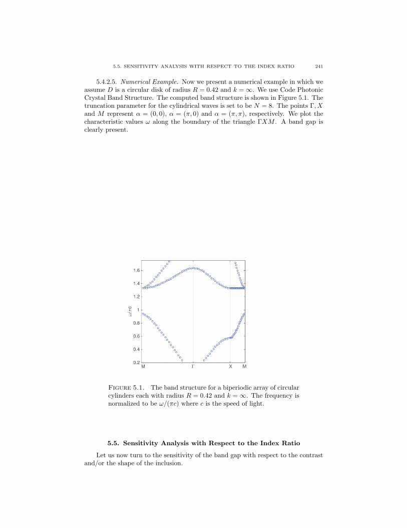
5.5. SENSITIVITY ANALYSIS WITH RESPECT TO THE INDEX RATIO 241
5.4.2.5. Numerical Example. Now we present a numerical example in which weassume D is a circular disk of radius R = 0.42 and k = ∞. We use Code PhotonicCrystal Band Structure. The computed band structure is shown in Figure 5.1. Thetruncation parameter for the cylindrical waves is set to be N = 8. The points Γ, Xand M represent α = (0, 0), α = (π, 0) and α = (π, π), respectively. We plot thecharacteristic values ω along the boundary of the triangle ΓXM . A band gap isclearly present.
Figure 5.1. The band structure for a biperiodic array of circularcylinders each with radius R = 0.42 and k = ∞. The frequency isnormalized to be ω/(πc) where c is the speed of light.
5.5. Sensitivity Analysis with Respect to the Index Ratio
Let us now turn to the sensitivity of the band gap with respect to the contrastand/or the shape of the inclusion.

242 5. PHOTONIC BAND GAPS
Expanding the operator-valued function Aα,k in terms of k and small pertur-bations of the shape of D, we calculate asymptotic expressions of its characteristicvalues with the help of the generalized Rouche theorem.
5.5.1. Preliminary Results. The following lemma, which is an immediateconsequence of (2.289), gives a complete asymptotic expansion of Aα,k as k → +∞.
Let Sα,ωl and (K−α,ωl )∗ be given by (2.289). Let the operators
Aα0 (ω) =
Sα,ω −Sα,0
01
2I + (K−α,0)∗
,
Aα1 (ω) =
0 −Sα,ω1(12I − (K−α,ω)∗
)(K−α,ω
1 )∗
,
and, for l ≥ 2,
Aαl (ω) =
(0 −Sα,ωl
0 (K−α,ωl )∗
).
Lemma 5.3. Suppose α 6= 0. We have
(5.19) Aα,k(ω) = Aα0 (ω) +
+∞∑
l=1
1
klAαl (ω).
We now have the following lemma for the characteristic values of Aα0 .
Lemma 5.4. Suppose α 6= 0. Then ωα0 ∈ R is a characteristic value of Aα0 if
and only if (ωα0 )2 is either an eigenvalue of −∆ in D with the Dirichlet boundary
condition or an eigenvalue of −∆ in Y \D with the Dirichlet boundary conditionon ∂D and the quasi-periodic condition on ∂Y .
Proof. Suppose that ω = ωα0 ∈ R is a characteristic value of Aα0 . Then there
is (φ, ψ) 6= 0 such that
(5.20)
Sα,ω[φ]− Sα,0[ψ] = 0,(12I + (K−α,0)∗
)[ψ] = 0
on ∂D.
It then follows from Lemma 2.94 that ψ = 0 and hence Sα,ω[φ] = 0 on ∂D. Sinceφ 6= 0, Sα,ω[φ] 6= 0 either in D or in Y \D and hence (ωα0 )
2 is either an eigenvalueof −∆ in D with the Dirichlet boundary condition or an eigenvalue of −∆ in Y \Dwith the Dirichlet boundary condition on ∂D and the quasi-periodic condition on∂Y , and Sα,ω[φ] is an associated eigenfunction.
Conversely if (ωα0 )2 is an eigenvalue of −∆ in D with the Dirichlet boundary
condition, then by Green’s representation formula, we have
u(x) = −Sα,ω[∂u∂ν
∣∣∣∂D
], x ∈ D.
Thus (5.20) holds with (φ, ψ) = (∂u/∂ν|∂D, 0). The other case can be treatedsimilarly using (2.290). This completes the proof.

5.5. SENSITIVITY ANALYSIS WITH RESPECT TO THE INDEX RATIO 243
At this moment let us invoke the results in [263] (see also [221, 262, 428]).In [263], it is shown, by a completely different argument which involves the conver-gence of quadratic forms, that the spectrum of (5.6) for α 6= 0 accumulates near thespectrum of −∆ in D with the Dirichlet boundary condition on ∂D as k → +∞.According to this result, the eigenvalue of the exterior problem is not realized asa limit of eigenvalues of the problem (5.6). In fact, the limit of the correspondingeigenfunctions is given by
u(x) =
Sα,ω[φ], x ∈ D,
Sα,0[ψ] = 0, x ∈ Y \D,where the pair (φ, ψ) is defined by (5.20). If (ωα0 )
2 is an eigenvalue for the exteriorproblem and not for the interior problem, then Sα,ω[φ] = 0 in D and hence u = 0in Y .
The following lemma was first proved in [263, 262].
Lemma 5.5. Let (ω0)2 (with ω0 > 0) be a simple eigenvalue of −∆ in D withthe Dirichlet boundary condition. There exists a unique eigenvalue (ωα,k)2 (withωα,k > 0) of (5.6) lying in a small complex neighborhood V of ω0. Indeed, ω0 andωα,k are simple poles of (Aα
0 )−1 and (Aα,k)−1, respectively.
5.5.2. Full Asymptotic Expansion. Combining now the generalized Rouchetheorem together with Lemma 5.3, we are able to derive complete asymptotic for-mulas for the characteristic values of ω 7→ Aα,k(ω). Applying Theorem 1.14 yieldsthat
ωα,k − ω0 =1
2√−1π
tr
∫
∂V
(ω − ω0)(Aα,k)−1(ω)d
dωAα,k(ω)dω.
Suppose that the quasi-momentum α 6= 0. We obtain the following complete as-ymptotic expansion for the eigenvalue perturbations ωα,k − ω0.
Theorem 5.6. Let V be as in Lemma 5.5. Suppose α 6= 0. Then the followingasymptotic expansion holds:
(5.21) ωα,k − ω0 =1
2√−1π
+∞∑
p=1
1
p
+∞∑
n=p
1
kntr
∫
∂V
Bαn,p(ω)dω,
where
(5.22) Bαn,p(ω) = (−1)p∑
n1+...+np=n
ni≥1
(Aα0 )
−1(ω)Aαn1(ω) . . . (Aα
0 )−1(ω)Aα
np(ω)
and
(5.23) (Aα0 )
−1(ω) =
(Sα,ω)−1 (Sα,ω)−1Sα,0(12I + (K−α,0)∗)−1
0 (1
2I + (K−α,0)∗)−1
.
5.5.3. Leading-Order Term. Let us compute the leading-order term in theexpansion of ωα,k − ω0. Let u0 be the (normalized) eigenvector associated to thesimple eigenvalue (ω0)2 and let ϕ := ∂u0/∂ν|− so that
(5.24) u0(x) = −Sα,ω0
[ϕ](x) for x ∈ D.
We first establish the following lemma.

244 5. PHOTONIC BAND GAPS
Lemma 5.7. The following identity holds:
(5.25)⟨ϕ,
d
dωSα,ω[ϕ]
∣∣ω=ω0
⟩= −2ω0
∫
D
|u0|2.
Proof. From (2.278), it follows that
∆d
dωGα,ω(x, y) + ω2 d
dωGα,ω(x, y) = −2ωGα,ω(x, y),
and therefore,
d
dωGα,ω(x, y) = −2ω
∫
Y
Gα,ω(x, z)Gα,ω(z, y)dz.
Consequently, for any ψ ∈ L2(∂D),
dSα,ω[ψ](x)dω
=d
dω
∫
∂D
Gα,ω(x, y)ψ(y) dσ(y)
=
∫
∂D
d
dωGα,ω(x, y)ψ(y) dσ(y)
=− 2ω
∫
Y
Gα,ω(x, z)
∫
∂D
Gα,ω(z, y)ψ(y) dσ(y)dz
=− 2ω
∫
Y
Gα,ω(x, z)Sα,ω[ψ](z)dz.
Using the fact that
Sα,ω0
[ϕ] =
−u0 in D,0 in Y \D,
we compute
⟨ϕ,dSα,ω[ϕ]dω
∣∣∣∣ω=ω0
⟩=
∫
∂D
ϕ(x)dS−α,ω
dω[ϕ](x)
∣∣∣∣ω=ω0
dσ(x)
= −2ω0
∫
∂D
ϕ(x)
∫
Y
Gα,ω0
(x, z)S−α,ω0
[ϕ](z)dz dσ(x)
= −2ω0
∫
∂D
∫
∂D
∫
Y
Gα,ω0
(x, z)G−α,ω0
(y, z)ϕ(x)ϕ(y)dzdσ(x) dσ(y)
= −2ω0
∫
Y
∣∣∣∣∫
∂D
Gα,ω0
(x, z)ϕ(x)dσ(x)
∣∣∣∣2
dz
= −2ω0
∫
Y
∣∣∣∣Sα,ω0
[ϕ](z)
∣∣∣∣2
dz
= −2ω0
∫
D
|u0(z)|2 dz,
which yields the desired formula.
We are now ready to prove the following theorem.
Theorem 5.8. Let vα be the unique α-quasi-periodic solution to
(5.26)
∆vα = 0 in Y \D,∂vα
∂ν
∣∣∣+=∂u0
∂ν
∣∣∣−
on ∂D.

5.5. SENSITIVITY ANALYSIS WITH RESPECT TO THE INDEX RATIO 245
The following asymptotic expansion holds:
(5.27) ωα,k − ω0 = −1
k
∫
Y \D|∇vα|2
2ω0
∫
D
|u0|2+O(
1
k2) as k → +∞.
Proof. Because of (5.24), we get
(1
2I − (K−α,ω0
)∗)[ϕ] = ϕ.
Moreover, since ω0 is the only simple pole in V of the mapping ω 7→ (Sα,ω)−1, wecan write [79]
(Sα,ω)−1 =1
ω − ω0T +Qα,ω,
where the operator-valued function Qα,ω is holomorphic in ω in V , T : L2(∂D) →spanϕ is such that TSα,ω0
= Sα,ω0
T = 0, and
Td
dωSα,ω
∣∣∣∣ω=ω0
=1
||ϕ||2L2
〈ϕ, ·〉ϕ
is the orthogonal projection from L2(∂D) into spanϕ. Here (·, ·) is the L2-innerproduct on ∂D. It can also be shown that
(5.28) T =1
⟨ϕ,
d
dωSα,ω[ϕ]
∣∣ω=ω0
⟩⟨ϕ, ·⟩ϕ.
It then follows from the residue theorem that
1
2√−1π
tr
∫
∂V
(Aα0 )
−1(ω)Aα1 (ω)dω = tr
[TSα,0
(12I+(K−α,0)∗
)−1(12I−(K−α,ω0
)∗)].
Let
vα(x) := Sα,0(12I + (K−α,0)∗
)−1[ϕ](x), x ∈ Y \D.
Then vα is the unique α-quasi-periodic solution to (5.26) and
1
2√−1π
tr
∫
∂V
(Aα0 )
−1(ω)Aα1 (ω)dω =
1
||ϕ||2L2
〈ϕ, Tvα〉.
Therefore, we have from (5.21)
ωα,k − ω0 = − 1
k||ϕ||2L2
〈ϕ, Tvα〉+O(1
k2) as k → +∞.
By virtue of (5.28), it follows that
1
||ϕ||2L2
〈ϕ, Tvα〉 = 1⟨ϕ,
d
dωSα,ω[ϕ]
∣∣ω=ω0
⟩⟨ϕ, vα
⟩.
Integration by parts yields
〈ϕ, vα〉 = −∫
Y \D|∇vα|2,
and hence we obtain (5.27) from Lemma 5.7. This completes the proof.

246 5. PHOTONIC BAND GAPS
Note that if u0 is normalized, then (5.27) can be rewritten as
(5.29) (ωα,k)2 − (ω0)2 = −1
k
∫
Y \D|∇vα|2 +O(
1
k2) as k → +∞.
5.5.4. Periodic Case. Turning now to the periodic case (α = 0), we firstintroduce the following notation. Let χY denote the constant function 1 on Y . Let
the operator ∆ be acting on spanχ(Y ), H10 (D), with
(5.30) ∆u :=
−∆(u|D) in D,
1
|Y \D|
∫
∂D
∂
∂ν(u|D) in Y \D.
See [263]. It is worth mentioning that the eigenvalue problem for ∆ can be writtenas
∆u+ ω2u = 0 in D,
u+1
|Y \D|
∫
D
u = 0 on ∂D.
Define the sequence of operator-valued functions (A0l )l∈N by
(5.31) A00(ω) =
S0,ω − 1
ω2
∫
∂D1
2I − (K0,ω)∗
1
2I + (K0,0)∗
,
(5.32) A01(ω) =
(0 −S0,0
0 (K0,ω1 )∗
), A0
l (ω) =
(0 −S0,ω
l−1
0 (K0,ωl )∗
)
for l ≥ 2, and set
(5.33) B0n,p(ω) = (−1)p
∑
n1+...+np=n
ni≥1
(A00)
−1(ω)A0n1(ω) . . . (A0
0)−1(ω)A0
np(ω).
Here, the operators S0,ωl and (K0,ω
l )∗ are given by (2.289) with α = 0.
The following complete asymptotic expansion of A0,k as k → +∞ holds:
A0,k(ω) = A00(ω) +
+∞∑
l=1
1
klA0l (ω).
On the other hand, we have the following lemma on the characteristic value of A00,
whose proof will be given in Section 5.9.
Lemma 5.9. Suppose that (ω0)2 (with ω0 > 0) is not an eigenvalue of −∆ inY \D with Dirichlet boundary condition on ∂D and the periodic condition on ∂Y .
Then (ω0)2 is an eigenvalue of ∆ if and only if ω0 is a characteristic value of the
operator-valued function A00.
Analogously to Theorem 5.6, the asymptotic formula for α = 0 follows from adirect application of Theorem 1.14.

5.5. SENSITIVITY ANALYSIS WITH RESPECT TO THE INDEX RATIO 247
Theorem 5.10. Suppose α = 0. Let (ω0)2 (with ω0 > 0) be a simple eigenvalue
of ∆. There exists a unique eigenvalue (ω0,k)2 (with ω0,k > 0) of (5.6) lying in asmall complex neighborhood of (ω0)2 and the following asymptotic expansion holds:
(5.34) ω0,k − ω0 =1
2√−1π
+∞∑
p=1
1
p
+∞∑
n=p
1
kntr
∫
∂V
B0n,p(ω)dω,
where V is a small complex neighborhood of ω0 and B0n,p(ω) is given by (5.33).
5.5.5. The case when |α| is of order 1/√k. In this subsection we derive
an asymptotic expansion which is valid for |α| of order O(1/√k), not just for fixed
α 6= 0 or α = 0, as has been considered in the previous subsections. We give thelimiting behavior of ωα,k in this case.
Recall that we seek for the characteristic value of the operator-valued functionω 7→ Aα,k(ω) where Aα,k(ω) is given in (5.13). One of the difficulties in dealing
with the operator when |α| is of order 1/√k is that Aα,k(ω) has a singularity at
ω2 = |α|2/k as one can see from the first formula in Subsection 2.13.1. In orderto avoid this difficulty, we use an argument different from those in the previoussections.
Note that finding a characteristic value of Aα,k(ω) is equivalent to finding anonzero (ϕ, ψ) satisfying
(5.35)
Sα,ω[ϕ]− Sα,ω√k [ψ] = 0,
1
k
(1
2I − (K−α,ω)∗
)[ϕ] +
(1
2I + (K−α, ω√
k )∗)[ψ] = 0
on ∂D. If such a pair (ϕ, ψ) exists, then ϕ 6= 0. In fact, if ϕ = 0, then
Sα,ω√k [ψ] = 0 and
∂Sα,ω√k [ψ]
∂ν
∣∣∣∣+
=
(1
2I + (K−α, ω√
k )∗)[ψ] = 0 on ∂D.
If k is so large that ω2/k is not a Dirichlet eigenvalue on D, then it follows that
Sα,ω√k [ψ] = 0 in D and Y \D, and hence ψ = 0. Therefore finding a nonzero (ϕ, ψ)
satisfying (5.35) amounts to finding a nonzero ϕ satisfying[(
1
2I − (K−α,ω)∗
)+ k
(1
2I + (K−α, ω√
k )∗)(Sα,
ω√k )−1Sα,ω
][ϕ] = 0
on ∂D. Thus finding a characteristic value of Aα,k(ω) is equivalent to finding acharacteristic value of the operator-valued function
(5.36) ω 7→(1
2I − (K−α,ω)∗
)+ kN
α, ω√kSα,ω,
where we put
(5.37) Nα, ω√
k :=
(1
2I + (K−α, ω√
k )∗)(Sα,
ω√k )−1.
Note that Nα, ω√
k can be extended to the Dirichlet-to-Neumann map for
∆ +ω2
kon Y \D

248 5. PHOTONIC BAND GAPS
with α-quasi-periodic condition on ∂Y , which is defined for
ω2
k< minα∈ ]−π,π]2
κ(α).
Here κ(α) is the smallest eigenvalue of −∆ with the Dirichlet boundary condition
on ∂D and quasi-periodicity on ∂Y . Furthermore, Nα, ω√
k depends smoothly bothon ω and α. Therefore, we have the expansion
Nα, ω√
k = Nα,0 +ω2
k
d
d(t2)Nα,t
∣∣t=0
+O
(1
k2
).
A further expansion in terms of α yields
(5.38) Nα, ω√
k = Nα,0 +ω2
kN +O
( |α|k
)+
(1
k2
),
where
(5.39) N :=d
d(t2)N0,t
∣∣t=0
.
The expansion (5.38) was first obtained by Friedlander [221].
In order to obtain a better understanding of the operator N , let us considerthe following problem for t small:
∆ut + t2ut = 0 in Y \D,ut = f on ∂D,
ut and∂ut∂ν
are periodic on ∂Y.
Since
N0,t[f ] =∂ut∂ν
|∂D,one can see that
(5.40) N [f ] =∂w
∂ν
∣∣∣∣∂D
,
where w = ∂ut/∂(t2)|∂D, which is the solution to
∆w + u0 = 0 in Y \D,w = 0 on ∂D,
w and∂w
∂νare periodic on ∂Y.
Using (5.40), we can derive relevant estimates for N . We have
‖N [f ]‖H−1/2(∂D) =
∥∥∥∥∂w
∂ν
∥∥∥∥H−1/2(∂D)
≤ C‖w‖H1(D) ≤ C ′‖u0‖H−1(D).
Therefore, we have for example
(5.41) ‖N [f ]‖H−1/2(∂D) ≤ C‖f‖H1/2(∂D).
It should be noted that the estimate (5.41) is not optimal.The following lemma will be useful.
5.5. SENSITIVITY ANALYSIS WITH RESPECT TO THE INDEX RATIO 249
Lemma 5.11. Let u1, u2, . . . be the eigenfunctions corresponding to 0 ≤ ωα,k1 ≤ωα,k2 ≤ . . .. For a given constant M there exists C such that
(5.42)
∥∥∥∥uj −1
|∂D|
∫
∂D
uj
∥∥∥∥H1/2(∂D)
≤ C
(|α|+ 1
k
)‖uj‖H1(D)
for all j satisfying ωα,kj ≤M . Furthermore,
(5.43)
∣∣∣∣∫
D
uiuj +
∫
∂D
N [ui|∂D]uj∣∣∣∣ ≤ C
(|α|+ 1
k
)‖ui‖H1(D)‖uj‖H1(D),
provided that ωα,ki 6= ωα,kj . If ωα,ki = ωα,kj for some i 6= j, then we can choose uiand uj in such a way that (5.43) holds.
Proof. We get from (5.38) that
N0,0
[uj −
1
|∂D|
∫
∂D
uj
]=
1
k
(∂uj∂ν
− (ωαj )2N [uj |∂D]
)
+ (N0,0 −Nα,0)[uj |∂D] +O(|α|) +O
(1
k
).
Note that N0,0 is the Dirichlet-to-Neuman map defined on ∂D for the Laplacianin Y \D with the periodic boundary condition on ∂Y , and hence it is invertible as
an operator from H1/20 (∂D) into H
−1/20 (∂D), where the subscript 0 indicates the
zero-mean value (in a weak sense for H−1/20 (∂D)). Since Nα,0 −N0,0 = O(|α|) as
an operator from H1/2(∂D) into H−1/2(∂D), (5.41) leads to∥∥∥∥uj −
1
|∂D|
∫
∂D
uj
∥∥∥∥H1/2(∂D)
≤ C
(|α|+ 1
k
)‖uj‖H1/2(∂D),
from which (5.42) follows.To prove (5.43), we introduce a notation for the quadratic form: Let
(5.44) E(u, v) :=
∫
D
∇u · ∇v dx.
Since Nα,ωα,ki is the Dirichlet-to-Neuman map for the exterior problem, it follows
from the divergence theorem that
(ωα,ki )2(∫
D
uiuj +
∫
∂D
N [ui|∂D]uj)
= E(ui, uj)−∫
∂D
(kNα,ωα,k
i − (ωα,ki )2N
)[ui|∂D]uj .
We also have
(ωα,kj )2(∫
D
ui · uj +∫
∂D
N [ui|∂D]uj)
= E(ui, uj)−∫
∂D
(ui kN
α,ωα,kj [uj |∂D]− (ωα,ki )2N [ui|∂D]
)uj
= E(ui, uj)−∫
∂D
(kNα,ωα,k
j − (ωα,kj )2N
)[ui|∂D]uj ,

250 5. PHOTONIC BAND GAPS
where the last equality holds thanks to the fact that the Dirichlet-to-Neuman mapis self-adjoint. Consequently,
((ωα,ki )2 − (ωα,kj )2
)(∫
D
uiuj +
∫
∂D
N [ui|∂D]uj)
=
∫
∂D
((kNα,ωα,k
j − (ωα,kj )2N)− (kNα,ωα,ki − (ωα,ki )2N)
)[ui|∂D]uj
=
∫
∂D
((kNα,ωα,k
j − kNα,0 − (ωα,kj )2N)
− (kNα,ωα,ki − kNα,0 − (ωα,ki )2N)
)[ui|∂D]uj .
Hence, (5.43) follows from (5.38), and the proof is complete.
The estimate (5.42) shows that if |α| and 1/k are small enough, then uj isalmost constant on ∂D, which is in good agreement with the case when α = 0.
5.6. Photonic Band Gap Opening
In this section we discuss the photonic band gap opening in the limiting caseas k tends to +∞. We will not include proofs in this section since very similar oneswill be given in Section 6.3.
Let ωj be the eigenvalues of −∆ in D with Dirichlet conditions and let ωj be
the eigenvalues of ∆ defined in (5.30). Then the following min-max characterizationof ωj and ωj is proved in [263] (see also Lemma 6.16):
(5.45) ω2j = min
Nj
maxu∈Nj ,‖u‖L2(D)=1
E(u, u),
and
(5.46) ω2j = min
Nj
maxu∈Nj ,‖u‖L2(D)=1
E(u, u)
1−∣∣∫
D
u∣∣2,
where the minimum is taken over all j -dimensional subspaces Nj of H10 (D) and
the quadratic form E is defined by (5.44). Using the min-max characterization, onecan show the following interlacing relation:
(5.47) ωj ≤ ωj ≤ ωj+1, j = 1, 2, . . . .
One can also show the following: For any ε > 0 and j, there exist c1 and c2sufficiently small such that we have
(5.48) ωj − ǫ ≤ ωα,kj+1 ≤ ωj+1
for |α| ≤ c1 and k > 1/c2. See Lemma 6.18.Since 0 is an eigenvalue of the periodic problem with multiplicity 1, combining
formulas (5.21), (5.34), and (5.48) shows that the spectral bands converge, as k →+∞, to
(5.49) [0, ω1] ∪ [ω1, ω2] ∪ [ω2, ω3] ∪ . . . ,and hence we have a band gap if and only if the following holds:
(5.50) ωj < ωj for some j.

5.7. SMALL PERTURBATIONS IN THE GEOMETRY OF THE HOLES 251
It is proved in [263] that the spectral bands converge to (5.49) in a somewhatdifferent way and (5.50) holds provided that
∫Duj 6= 0 where uj is an eigenfunction
corresponding to ω2j .
As we will see in the next chapter, the situation for the phononic crystal ismore subtle and complicated. Among other reasons, it is because, unlike the caseof the Laplace operator, 0 is an eigenvalue of the periodic problem for the Lamesystem with multiplicity 2 (in two dimensions).
5.7. Sensitivity Analysis with Respect to Small Perturbations in theGeometry of the Holes
Suppose that D is of class C2. Let Dǫ be an ǫ-perturbation of D; i.e., leth ∈ C1(∂D) and ∂Dǫ be given by
∂Dǫ =
x : x = x+ ǫh(x)ν(x), x ∈ ∂D
.
Define the operator-valued function Aαǫ by
Aαǫ : ω 7→
Sα,ωDǫ−Sα,
ω√k
Dǫ
1
k
(1
2I − (K−α,ω
Dǫ)∗)
1
2I + (K−α, ω√
k
Dǫ)∗
.
Write∂Gα,ω
∂ν(x)(x, y) =
1
2π
〈x− y, ν(x)〉|x− y|2 +Rα,ω(x, y),
where Rα,ω(x, y) is smooth for all x and y. Following Subsection 3.2.2, we have auniformly convergent expansion for the length element dσǫ(y) on ∂Dǫ; i.e.,
dσǫ(y) =+∞∑
n=0
ǫnσ(n)(y)dσ(y),
where σ(n) are bounded functions, and easily prove that the following lemma holds.
Lemma 5.12. Let Ψǫ be the diffeomorphism from ∂D onto ∂Dǫ given by Ψǫ(x) =x+ ǫh(x)ν(x). Let N ∈ N. There exist C depending only on N , the C2-norm of D,and ‖h‖C1(∂D) such that for any ϕ ∈ L2(∂Dǫ),
∥∥∥∥∥Sα,ωDǫ
[ϕ] Ψǫ − Sα,ω[ϕ]−N∑
n=1
ǫnS(n)α,ω[ϕ]
∥∥∥∥∥L2(∂D)
≤ CǫN+1||ϕ||L2(∂D)
and∥∥∥∥∥((K
−α,ωDǫ
)∗[ϕ]) Ψǫ − (Kα,ω)∗ϕ−N∑
n=1
ǫnK(n)α,ω[ϕ]
∥∥∥∥∥L2(∂D)
≤ CǫN+1‖ϕ‖L2(∂D),
where ϕ := ϕ Ψǫ. Here
S(n)α,ω[ϕ](x) =
n∑
l=0
∑
|β|=l
1
β!
∫
∂D
∂βGα,ω(x, y)(h(x)ν(x)−h(y)ν(y))lσ(n−l)(y)ϕ(y)dσ(y),

252 5. PHOTONIC BAND GAPS
and
K(n)α,ω[ϕ](x) = K(n)
ω [ϕ](x)
+
n∑
l=0
∑
|β|=l
1
β!
∫
∂D
∂βRα,ω(x, y)(h(x)ν(x)− h(y)ν(y))lσ(n−l)(y)ϕ(y) dσ(y),
and the bounded operators K(n)ω = K(n)
D,ω are defined in (2.146).
The sensitivity analysis with respect to small perturbations in the geometry ofthe holes consists of expanding, based on Lemma 5.12, Aα
ǫ in terms of ǫ to calculateasymptotic expressions of its characteristic values. This can be done in exactly thesame manner as in Theorem 5.6.
5.8. Proof of the Representation Formula
In this section we provide a proof of representation formula (5.10) which playsa central role in our analysis.
Theorem 5.13. Suppose that ω2 is not an eigenvalue for −∆ in Y \ D withDirichlet boundary condition on ∂D and quasi-periodic boundary condition on ∂Yand assume ω2/k is not an eigenvalue for −∆ in D with Dirichlet boundary condi-tion on ∂D. Then, for any eigenfunction u of (5.6), there exists one and only onepair (φ, ψ) ∈ L2(∂D)×L2(∂D) such that u has the representation (5.11). Moreover,(φ, ψ) is the solution to the integral equation (5.12). The mapping u 7−→ (φ, ψ) fromsolutions of (5.6) to solutions of the system of integral equations (5.12) is one-to-one.
We first prove the following lemma.
Lemma 5.14. Suppose that u is an eigenfunction of (5.6). Then
u|∂D ⊥ Ker(S−α,ω).
Here S−α,ω is considered an operator from L2(∂D) into H1(∂D).
Proof. To prove this lemma, we observe that, since (∆ + ω2)u = 0 in D,
u(x) = Dα,ω [u|∂D] (x)− Sα,ω[∂u
∂ν
∣∣∣−
](x), x ∈ D,
and consequently,
1
2u|∂D = Kα,ω [u|∂D]− Sα,ω
[∂u
∂ν
∣∣∣−
].
Let φ ∈ Ker(S−α,ω). Because of the assumption on ω2, we immediately deducethat S−α,ω[φ] = 0 in Y \D, and hence
(5.51)
S−α,ω[φ] = 0,
1
2φ+ (Kα,ω
)∗[φ] = 0
on ∂D.

5.8. PROOF OF THE REPRESENTATION FORMULA 253
Then, we have
1
2〈u|∂D, φ〉 = 〈Kα,ω [u|∂D] , φ〉 −
⟨Sα,ω
[∂u
∂ν
∣∣∣−
], φ
⟩
= 〈u|∂D, (Kα,ω)∗[φ]〉 −⟨∂u
∂ν
∣∣∣−,S−α,ω[φ]
⟩
= −1
2〈u|∂D, φ〉 − 0,
which proves the lemma.
Proof of Theorem 5.13. We first note that the problem of finding (φ, ψ) isequivalent to solving the two equations
(5.52)
Sα,ω[φ] = u|∂D on ∂D,(− 1
2I + (K−α,ω)∗
)[φ] =
∂u
∂ν
∣∣∣−
on ∂D
and
(5.53)
Sα,ω√k [ψ] = u|∂D on ∂D,
(12I + (K−α, ω√
k )∗)[ψ] =
∂u
∂ν
∣∣∣+
on ∂D.
Here we only consider the problem of finding φ, the solution to (5.52); the problemof finding ψ can be solved in the same way.
From Lemma 5.14 it follows that there exists φ0 ∈ L2(∂D) such that
Sα,ω[φ0 + φ] = u|∂D on ∂D, ∀φ ∈ Ker(Sα,ω).Hence, to show existence of a solution to (5.52), it suffices to prove that there existsφ ∈ Ker(Sα,ω) such that the second equation in (5.52) is satisfied by φ0+φ. Thanksto the second equation in (5.51), this equation becomes
(5.54) φ =∂ (Sα,ω[φ0]− u)
∂ν
∣∣∣−,
and then, we only need to show that
∂ (Sα,ω[φ0]− u)
∂ν
∣∣∣−∈ Ker(Sα,ω),
which is an immediate consequence of the fact that Sα,ω[φ0] − u is a solution to∆ + ω2 in D with the Dirichlet boundary condition. We have then proved theexistence of a solution to (5.52).
Suppose now that we have two solutions φ1 and φ2 to (5.52). Then, because ofthe assumption on ω2, we have Sα,ω[φ1 − φ2] = 0 in Y \D, and hence
(12I + (K−α,ω)∗
)[φ1 − φ2] = 0 on ∂D.
By the second equation in (5.52), we have φ1 = φ2.So far, we have shown that there are unique φ and ψ satisfying (5.52) and
(5.53), respectively. The jump conditions satisfied by u immediately show that thepair (φ, ψ) satisfies the system of integral equations (5.12).
Conversely, suppose that (φ, ψ) is a nontrivial solution to the system of integralequations (5.12). Then defining u by (5.11), we only need to show that u is nottrivial to conclude that u is an eigenfunction of (5.6). Suppose that u = 0 in Y .

254 5. PHOTONIC BAND GAPS
Then Sα,ω[φ] = 0 inD, and by the assumption on ω2, we deduce that Sα,ω[φ] = 0 inY \D. Finally, from the jump of the normal derivative of Sα,ω[φ] on ∂D, we deducethat φ = 0. The assumption on ω2/k leads to ψ = 0. This is in contradiction tothe fact that (φ, ψ) 6= (0, 0). This completes the proof.
5.9. Characterization of the Eigenvalues of ∆
Let ω0 be a characteristic value of the operator-valued function A00. Let (φ, ψ)
be a root function associated with ω0. Set
u = S0,ω[φ]− 1
ω20
∫
∂D
ψ
and
c =1
ω20 |Y \D|
∫
∂D
(−1
2I + (K0,ω)∗)[φ].
It follows from (2.291) that
c =1
ω20
∫
∂D
ψ,
and therefore, −∆(u + c) = ω20(u + c) in D and u = 0 on ∂D. Thus, we conclude
that ω20 is an eigenvalue of ∆.
Conversely, assume that ω20 (with ω0 > 0) is an eigenvalue of ∆ associated with
u+ c, where u ∈ H10 (D), and
c =1
|Y \D|ω20
∫
∂D
∂u
∂ν.
Let φ be a solution to
(5.55) (1
2I − (K0,ω0)∗)[φ] =
∂u
∂νon ∂D.
Such a solution exits even though ω20 is an eigenvalue of the Laplacian in D with
Neumann boundary condition since in this case ∂u/∂ν is orthogonal in L2 to theassociated Neumann eigenvector. Set
(5.56) ψ = −(1
2I + (K0,0)∗)−1
[∂u
∂ν
].
Then, (φ, ψ) satisfies
S0,ω0 − 1
ω20
∫
∂D
1
2I − (K0,ω0)∗
1
2I + (K0,0)∗
(φ
ψ
)= 0,
which proves that ω0 is a characteristic value of A00.
5.10. Maximizing Band Gaps in Photonic Crystals
Let Y denote the periodic unit cell [0, 1)2. To study the optimal design ofphotonic band gaps, we consider the quasi-periodic eigenvalue problems:
(5.57) − (∇+√−1α) · (∇+
√−1α)uα = (ωα)2q(x)uα
and
(5.58) − (∇+√−1α)
1
q(x)· (∇+
√−1α)vα = (ωα)2vα,

5.10. MAXIMIZING BAND GAPS IN PHOTONIC CRYSTALS 255
where α is in the Brillouin zone and the density function q(x) is given by
(5.59) q(x) =
q1 for x ∈ Ω \D,q2 for x ∈ D.
The eigenvalue problem (5.57) is for the transverse magnetic polarization while(5.58) is for the transverse electric polarization.
The spectrum of (5.57) (resp. (5.58)) is composed of a sequence of nonnegativeeigenvalues, each of finite multiplicity. Repeating them according to multiplicity,we denote them
0 ≤ ωα1 ≤ ωα2 ≤ ωα3 . . .→ +∞.
If we use the level set method (see Appendix B.2) to represent the interface∂D, then
q(x) =
q1 for x, φ(x) < 0,q2 for x, φ(x) > 0.
A typical design goal is to maximize the band gap in the transverse magneticor the transverse electric case. In both cases, we write [188, 289, 260, 162]
(5.60) J [D] = infαωαj+1 − sup
αωαj
and maximize J [D] with respect to the level set function φ. An analysis of theproblem shows that it may be nonsmooth, i.e., Lipschitz continuous but not differ-entiable with respect to φ, for several reasons [188]. First of all, the inf and sup inthe definition of J are nonsmooth functions. Moreover, multiple eigenvalues intro-duce a nondifferentiability with respect to φ. However, one can still use generalizedgradients and bundle optimization techniques to overcome this difficulty.
The generalized gradient of a locally Lipschitz function is defined as follows[179, Chapter 2]. Let X be a real Banach space and let f : X → R be Lipschitznear a given point x ∈ X. Define
f(x, v) := lim supy→x,t→0+
f(y + tv)− f(y)
t.
The generalized gradient of f at x, denoted ∂f(x), is the (nonempty) weak*-compact subset of X∗ (the dual space of continuous linear functionals on X) whose
support function is f(x, ·). Thus ζ ∈ ∂f(x) if and only if f(x, v) ≥ (ζ, v) for all vin X. It is also worth noticing that if f admits a Gateaux derivative f ′G(x) at x,then f ′G(x) ∈ ∂f(x). Moreover, if f is continuously differentiable at x, then ∂f(x)reduces to a singleton: ∂f(x) = f ′(x).
Let co denote the convex hull, i.e., the set of all convex combinations of elementsin the given set. Returning now to our optimal design problem, the generalizedgradient of ωαj with respect to φ can be written as follows [188, 289]:
∂φωαj ⊂ co
− 1
2(q2 − q1)ω
αj |uα|2 : uα ∈ V(j)
TM (q, α)
,
in the transverse magnetic case, and
∂φωαj ⊂ co
1
2ωαj(1
q2− 1
q1)|(∇+
√−1α)vα|2 : vα ∈ V(j)
TE(q, α)
,

256 5. PHOTONIC BAND GAPS
in the TE case, where V(j)TM (and V(j)
TE) are the span of all eigenfunctions uα (andvα) associated with the eigenvalue ωαj , respectively, and satisfying the normalization∫Yq|uα|2 = 1 and
∫Y|vα|2 = 1. The shape derivatives of J [D] are given by
dSJ [D] =
∫
∂D
VTM (or VTE) θ · ν dσ,
where the velocities which give the ascent direction for the optimization are [188,289]
(5.61)
VTM ⊂ co
− 1
2(q2 − q1)ω
αj+1|uα|2 : uα ∈ V(j+1)
TM (q, α)
−co
− 1
2(q2 − q1)ω
αj |uα|2 : uα ∈ V(j)
TM (q, α)
and
(5.62)
VTE ⊂ co
1
2ωαj+1
(1
q2− 1
q1)|(∇+
√−1α)vα|2 : vα ∈ V(j+1)
TE (q, α)
−co
1
2ωαj(1
q2− 1
q1)|(∇+
√−1α)vα|2 : vα ∈ V(j)
TE(q, α)
.
5.11. Photonic Cavities
Let k be a positive constant and let k(x) be a periodic function with period 1in x1 and x2 such that
k(x) =
k in Y \D,1 in D.
Consider the solution u to the following problem:
(5.63) ∇ · k(x)∇u+ ω2n(x)u = 0.
Suppose that n(x) − 1 is compactly supported in a bounded domain Ω ⊂ R2, andis assumed to be known. Assume that Ω is a localized defect inserted into thephotonic crystal. It can be proved that the introduction of a localized defect doesnot change the essential spectrum of the operator.
Assume that the operator ∇ · k(x)∇ has a gap in the spectrum and seek for ωinside the bandgap such that (5.63) has a nontrivial solution. As in Section 3.3, wecan use an integral formulation to compute ω. We can formally rewrite the solutionto (5.63) in integral form
(5.64) u(x) + ω2
∫
Ω
(n(y)− 1)Gω(x, y)u(y)dy = 0 , x ∈ R2,
where Gω is the Green’s function of ∇·k(x)∇+ω2 in R2. Notice that for frequenciesin the band gap, Gω is exponentially decaying. We have [183]
(5.65) |Gω(x, y)| = O(e−Cdist(ω2,σ(−∇·k(x)∇))
)as |x− y| → ∞
with C being a positive constant and σ(−∇·k(x)∇) is the spectrum of −∇·k(x)∇.We call ω a defect mode if its value in (5.64) yields nontrivial solutions u(x) of
(5.64). Hence, in view of (5.65), a defect mode is a solution to the wave equationwhich is exponentially localized in the defect while its time dependence is har-monic and can be computed by the same approach as the one presented in Section3.3. Moreover, using the generalized argument principle, we can also compute thesensitivity of the defect modes with respect to n and Ω.

5.12. CONCLUDING REMARKS 257
5.12. Concluding Remarks
In this chapter we have first discussed the structure of spectra of periodicelliptic operators. The main tool of the theory is the Floquet transform. Wehave also performed a high-order sensitivity analysis of the spectral properties ofhigh contrast band gap materials, consisting of a background medium which isperforated by a periodic array of holes, with respect to the index ratio and smallperturbations in the geometry of the holes. The asymptotic expansions have beenobtained by transforming the spectral problem into a system of equations involvingsingular integral operators, a Taylor expansion of the associated kernels, and thegeneralized Rouche theorem. The leading-order terms in our expansions have beenexplicitly computed.
Our approach in this chapter will be extended in the next chapter to the equa-tions of linear elasticity.


CHAPTER 6
Phononic Band Gaps
6.1. Introduction
In the past decade there has been a steady growth of interest in the propaga-tion of elastic waves through inhomogeneous materials. The ultimate objective ofthese investigations has been the design of the so-called phononic band gap ma-terials or phononic crystals. The most recent research in this field has focusedon theoretical and experimental demonstrations of band gaps in two-dimensionaland three-dimensional structures constructed of high contrast elastic materials ar-ranged in a periodic array. This type of structure prevents elastic waves in certainfrequency ranges from propagating and could be used to generate frequency filterswith control of pass or stop bands, as beam splitters, as sound or vibration protec-tion devices, or as elastic waveguides. See, for example, [454, 189, 310, 432].
To mathematically formulate the problem investigated in this chapter, set Dto be a connected domain with Lipschitz boundary lying inside the open square(0, 1)2. As in Chapter 5, an important example of phononic crystals consists of abackground elastic medium of constant Lame parameters λ and µ which is perfo-rated by an array of arbitrary-shaped inclusions Ω =
⋃n∈Z2(D+ n) periodic along
each of the two orthogonal coordinate axes in the plane. These inclusions have
Lame constants λ, µ. The shear modulus µ of the background medium is assumedto be larger than that of the inclusion µ. Then we investigate the spectrum of theself-adjoint operator defined by
(6.1) u 7→ −∇ · (C∇u) = −2∑
j,k,l=1
∂
∂xj
(Cijkl
∂uk∂xl
),
which is densely defined on L2(R2)2. Here the elasticity tensor C is given by
(6.2) Cijkl :=
(λχ(R2\Ω)+λ χ(Ω)
)δijδkl+
(µχ(R2\Ω)+µ χ(Ω)
)(δikδjl+δilδjk),
where χ(Ω) is the indicator function of Ω.In this chapter we adopt this specific two-dimensional model to understand the
relationship between the contrast of the shear modulus and the band gap structureof the phononic crystal. We will also consider the case of two materials with differentdensities in order to investigate the relation between the density contrast and theband gap structure.
By Floquet theory in Section 5.2, the spectrum of the Lame system with pe-riodic coefficients is represented as a union of bands, called the phononic bandstructure. Carrying out a band structure calculation for a given phononic crystalinvolves a family of eigenvalue problems, as the quasi-momentum is varied over thefirst Brillouin zone. The problem of finding the spectrum of (6.1) is reduced to a
259

260 6. PHONONIC BAND GAPS
family of eigenvalue problems with quasi-periodicity condition; i.e.,
∇ · (C∇u) + ω2u = 0 in R2,(6.3)
with the periodicity condition
(6.4) u(x+ n) = e√−1α·nu(x) for every n ∈ Z2.
Here the quasi-momentum α varies over the Brillouin zone [0, 2π)2. Each of theseoperators has compact resolvent so that its spectrum consists of discrete eigenvaluesof finite multiplicity. We show that these eigenvalues are the characteristic values ofmeromorphic operator-valued functions that are of Fredholm type of index zero. Asin Chapter 5, this yields a natural and efficient approach to the computation of theband gap phononic structure which is based on a combination of boundary elementmethods and Muller’s method for finding complex roots of scalar equations. SeeSection 1.6. Following Chapter 5, we proceed from the generalized Rouche theoremto construct complete asymptotic expressions for the characteristic values as theLame parameter µ of the background goes to infinity. For α 6= 0, we prove that thediscrete spectrum of (6.3) accumulates near the Dirichlet eigenvalues of the Lamesystem in D as µ goes to infinity. We then obtain a full asymptotic formula for theeigenvalues. The leading-order term is of order µ−1 and can be calculated explicitly.For the periodic case α = 0, we establish a formula for the asymptotic behaviorof the eigenvalues. It turns out that their limiting set is generically different fromthat for α 6= 0. We also consider the case when |α| is of order 1/√µ and derive anasymptotic expansion for the eigenvalues in this case as well. Not surprisingly, thisformula tends continuously to the previous ones as α
õ goes to zero or to infinity.
We finally provide a criterion for exhibiting gaps in the band structure. As wesaid before, the existence of those spectral gaps implies that the elastic waves inthose frequency ranges are prohibited from travelling through the elastic body. Ourcriterion shows that the smaller the density of the matrix, the wider the band gap,provided that the criterion is fulfilled. This phenomenon was reported in [205]where it was observed that periodic elastic composites, whose matrix has lowerdensity and higher shear modulus compared to those of inclusions, yield betteropen gaps.
6.2. Asymptotic Behavior of Phononic Band Gaps
The phononic crystal we consider in this chapter is a homogeneous elasticmedium of Lame constants λ, µ which contains a periodic (with respect to thelattice Z2) array of arbitrary-shaped inclusions Ω =
⋃n∈Z2(D + n). These inclu-
sions have Lame constants λ, µ.We use the same notation as in Chapter 5. Let Y = (0, 1)2 denote the fun-
damental periodic cell. For each quasi-momentum α ∈ [0, 2π)2, set σα(D) to bethe (discrete) spectrum of the operator defined by (6.1) with the condition that
6.2. ASYMPTOTIC BEHAVIOR OF PHONONIC BAND GAPS 261
e−√−1α·xu is periodic. In other words, σα(D) is the spectrum of the problem
(6.5)
Lλ,µu+ ω2u = 0 in Y \D,Lλ,µu+ ω2u = 0 in D,
u∣∣+− u
∣∣− = 0 on ∂D,
∂u
∂ν
∣∣+− ∂u
∂ν
∣∣− = 0 on ∂D,
e−√−1α·xu is periodic in the whole space.
Recall that Lλ,µ denotes the elastostatic system corresponding to the Lame con-
stants λ and µ and ∂/∂ν is the corresponding conormal derivative.By the standard Floquet theory briefly described in Subsection 5.2, the spec-
trum of (6.5) has the band structure given by
(6.6)⋃
α∈[0,2π)2
σα(D).
The main objective of this section is to investigate the behavior of σα(D) as µ →+∞.
6.2.1. Integral Representation of Quasi-Periodic Solutions. In this sub-section, we obtain the integral representation formula for the solution to (6.5). We
denote by Sω, Dω, and Kω the layer potentials on ∂D associated with the Lame
parameters (λ, µ).We first prove the following lemma.
Lemma 6.1. Suppose that ω2 is not an eigenvalue for −Lλ,µ in D with theDirichlet boundary condition on ∂D. Let u be a solution to (6.5). Then we have
u|∂D ⊥ Ker Sω and u|∂D ⊥ Ker(Sα,ω)∗.Here Sω and Sα,ω are considered to be operators on L2(∂D)2.
Proof. We first observe that, since (Lλ,µ + ω2)u = 0 in D, we have
(6.7) u(x) = Dω [u|∂D] (x)− Sω[∂u
∂ν
∣∣∣−
](x), x ∈ D,
and consequently by (2.156) it follows that
(6.8)1
2u|∂D = Kω [u|∂D]− Sω
[∂u
∂ν
∣∣∣−
].
Let φ ∈ Ker(Sω); i.e., Sω[φ] = 0 on ∂D. By Lemma 2.123, we have Sω[φ] = 0
in R2 \D and hence (1/2)φ+ (Kω)∗[φ] = 0 by (2.155). Then we have from (6.8)
1
2〈u|∂D, φ〉 =
⟨Kω [u|∂D] , φ
⟩−⟨Sω[∂u
∂ν
∣∣∣−
], φ
⟩
=⟨u|∂D, (Kω)∗[φ]
⟩−⟨∂u
∂ν
∣∣∣−, Sω[φ]
⟩
= −1
2〈u|∂D, φ〉 ,
which implies 〈u|∂D, φ〉 = 0, and hence u|∂D ⊥ Ker Sω.

262 6. PHONONIC BAND GAPS
Observe that if u is α-quasi-periodic, then
Dα,ωY [u|∂Y ] = 0 and Sα,ωY
[∂u
∂ν
∣∣∣+
]= 0 on ∂Y,
where Dα,ωY and Sα,ωY are the (α-quasi-periodic) double- and single-layer potentials
on ∂Y . Thus we have
u(x) = −Dα,ω [u|∂D] (x) + Sα,ω[∂u
∂ν
∣∣∣+
](x), x ∈ Y \D,
and consequently,
1
2u|∂D = −Kα,ω [u|∂D] + Sα,ω
[∂u
∂ν
∣∣∣+
].
Let φ ∈ Ker(Sα,ω)∗. Since (Sα,ω)∗ = S−α,ω, we have
S−α,ω[φ] = 0 on ∂D.
Since ω2 is not a Dirichlet eigenvalue of −Lλ,µ in D, we immediately get
S−α,ω[φ] = 0 in D,
and hence
−1
2φ+ (Kα,ω
)∗[φ] = 0 on ∂D.
Therefore, we can deduce that
1
2〈u|∂D, φ〉 = −〈Kα,ω [u|∂D] , φ〉+
⟨Sα,ω
[∂u
∂ν
∣∣∣+
], φ
⟩
= −〈u|∂D, (Kα,ω)∗[φ]〉+⟨∂u
∂ν
∣∣∣+,S−α,ω[φ]
⟩
= −1
2〈u|∂D, φ〉 ,
which implies 〈u|∂D, φ〉 = 0. This completes the proof.
We now establish a representation formula for solutions of (6.5).
Theorem 6.2. Suppose that ω2 is not an eigenvalue for −Lλ,µ in D with theDirichlet boundary condition on ∂D. Then, for any solution u of (6.5), there existsone and only one pair (φ, ψ) ∈ L2(∂D)2 × L2(∂D)2 such that
(6.9) u(x) =
Sω[φ](x), x ∈ D,
Sα,ω[ψ](x), x ∈ Y \D.Moreover, (φ, ψ) satisfies
(6.10)
Sω[φ]− Sα,ω[ψ] = 0 on ∂D,(12I − (Kω)∗
)[φ] +
(12I + (K−α,ω)∗
)[ψ] = 0 on ∂D,
and the mapping u 7−→ (φ, ψ) from solutions of (6.5) in H1(Y )2 to solutions to thesystem of integral equations (6.10) in L2(∂D)2 × L2(∂D)2 is a one-to-one corre-spondence.
6.2. ASYMPTOTIC BEHAVIOR OF PHONONIC BAND GAPS 263
Proof. We first note that the problem of finding (φ, ψ) satisfying (6.9) and(6.10) is equivalent to solving the following two systems of equations:
(6.11)
Sω[φ] = u|∂D on ∂D,(− 1
2I + (Kω)∗
)[φ] =
∂u
∂ν
∣∣∣−
on ∂D
and
(6.12)
Sα,ω[ψ] = u|∂D on ∂D,(12I + (K−α,ω)∗
)[ψ] =
∂u
∂ν
∣∣∣+
on ∂D.
In order to find φ satisfying (6.11), it suffices to find φ satisfying Sω[φ] = u inD. Suppose for a moment that the following holds:
(6.13) ℑSω =
φ : φ ⊥ Ker Sω
.
It then follows from Lemma 6.1 that there exists φ0 ∈ L2(∂D)2 such that
(6.14) Sω[φ0] = u|∂D on ∂D.
Observe that if ω 6= 0, then the solution to the Dirichlet problem for Lλ,µ+ω2 may
not be unique, and hence (6.14) does not imply Sω[φ0] = u in D. However, since
(Lλ,µ + ω2)(u− Sω[φ0]) = 0 in D, we get by Green’s formula
u− Sω[φ0] = −Sω[∂
∂ν
(u− Sω[φ0]
) ∣∣∣−
]in D,
and therefore,
u = Sω[φ0 −
∂
∂ν
(u− Sω[φ0]
) ∣∣∣−
]in D.
To prove the uniqueness of φ satisfying (6.11), it suffices to show that thesolution to
Sω[φ] = 0 on ∂D,(− 1
2I + (Kω)∗
)[φ] = 0 on ∂D
is zero. By the first equation in the above and Lemma 2.123, Sω[φ] = 0 in R2 \Dand hence
φ =∂
∂νSω[φ]
∣∣∣+− ∂
∂νSω[φ]
∣∣∣−= 0.
Similarly, we can show existence and uniqueness of ψ satisfying
u = Sα,ω[ψ] in Y \D,which yields (6.12). To complete the proof, we shall verify that (6.13) holds. LetG be a subspace of H1(∂Ω) such that
G :=
φ : φ ⊥ Ker Sω
.
Since〈Sωφ, ψ〉 = 〈φ, Sωψ〉, ∀φ, ψ ∈ L2(∂Ω),
it is easy to see that ℑ Sω ⊂ G. It remains then to show that
dimH1(∂Ω)/ℑ Sω ≤ dimH1(∂Ω)/G.
264 6. PHONONIC BAND GAPS
Let φ1, φ2, . . . , φn be an orthonormal basis of Ker Sω. Since H1(∂Ω) is dense in
L2(∂Ω), we can take φ1, φ2, . . . , φn in H1(∂Ω) such that ‖φj − φj‖L2(∂Ω) ≤ ǫ for all
j. Then φ1, φ2, . . . , φn is linearly independent in H1(∂Ω)/G. To see this, supposethat
a1φ1 + · · ·+ anφn ∈ G.
By taking the inner products with the φj ’s, we obtainφ1 · φ1 . . . φ1 · φn
...
φn · φ1 . . . φn · φn
a1...an
= 0.
Since φ1 · φ1 . . . φ1 · φn
...
φn · φ1 . . . φn · φn
is invertible (as it is a small perturbation of the identity), we have a1 = . . . = an = 0.Hence,
dimH1(∂Ω)/ℑ Sω = dim Ker Sω ≤ dimH1(∂Ω)/G,
and we can conclude that G = ℑ Sω.
Let Aα,µ(ω) be the operator-valued function of ω defined by
(6.15) Aα,µ(ω) :=
Sω −Sα,ω1
2I − (Kω)∗ 1
2I + (K−α,ω)∗
.
By Theorem 6.2, ω2 is an eigenvalue corresponding to the quasi-momentum α ifand only if ω is a characteristic value of Aα,µ(ω). Consequently, we now have a newway of computing the spectrum of (6.5) parallel to our formulation in the previouschapter of the band structure problem for photonic crystals. This way consistsof examining the characteristic values of Aα,µ(ω). Based on Muller’s method forfinding complex roots of scalar equations, a boundary element method similar tothe one developed in Subsection 5.4.2 for photonic crystals can be designed forcomputing phononic band gaps.
6.2.2. Full Asymptotic Expansions. Expanding the operator-valued func-tions Aα,µ(ω) in terms of µ as µ → +∞, we can calculate asymptotic expressionsof their characteristic values with the help of the generalized Rouche theorem, andthis is what we do in this subsection.
We begin with the following asymptotic expansion of Gα,ωij (x, y) in (2.524).
Lemma 6.3. Let τl = 1− (cT /cL)2l. As µ→ +∞,
(6.16)
Gα,ωij (x, y) =
+∞∑
l=1
ω2(l−1)
µl
∑
n∈Z2
e√−1(2πn+α)·(x−y)
( −δij|2πn+ α|2l
+τl(2πn+ α)i(2πn+ α)j
|2πn+ α|2(l+1)
),

6.2. ASYMPTOTIC BEHAVIOR OF PHONONIC BAND GAPS 265
for fixed α 6= 0, while for α = 0,
G0,ωij (x, y) =
δijω2
++∞∑
l=1
ω2(l−1)
(2π)2lµl
∑
n∈Z2\0e2π
√−1n·(x−y)(− δij|n|2l + τl
ninj|n|2(l+1)
).
(6.17)
The derivations of (6.16) and (6.17) are straightforward. In fact, since
1
k2T − |2πn+ α|2 =1
ω2
µ− |2πn+ α|2
= −+∞∑
k=0
ω2k
µk|2πn+ α|2(k+1),
one easily shows that (6.16) and (6.17) hold.We can write (6.16) and (6.17) as
(6.18) Gα,ω(x, y) =
+∞∑
l=1
1
µlGα,ωl (x, y)
and
(6.19) G0,ω(x, y) =1
ω2I +
+∞∑
l=1
1
µlG0,ωl (x, y),
where the definitions of Gα,ωl (x, y) and G0,ω
l (x, y) are obvious from (6.16) and
(6.17). We note that Gα,ωl (x, y) and G0,ω
l (x, y) are dependent upon µ becauseof the factor τl. However, since |τl| ≤ C for some constant C independent of µand l, this will not affect our subsequent analysis. We also note that Gα,ω
1 (x, y) isindependent of ω and
(6.20) Gα,ω1 (x, y) = µGα,0(x, y),
where Gα,0(x, y) is the quasi-periodic fundamental function defined in (2.525).
Denote by Sα,ωl and (K−α,ωl )∗, for l ≥ 1 and α ∈ [0, 2π)2, the single-layer
potential and the boundary integral operator associated with the kernel Gα,ωl (x, y)
as defined in (2.532) so that
(6.21) Sα,ω =
+∞∑
l=1
1
µlSα,ωl and (K−α,ω)∗ =
+∞∑
l=1
1
µl(K−α,ω
l )∗.
Lemma 6.4. The operator (1/2) I + (K−α,0)∗ : L2(∂D)2 → L2(∂D)2 is invert-ible.
Before proving Lemma 6.4, let us make a note of the following simple fact: Ifu and v are α-quasi-periodic, then
(6.22)
∫
∂Y
∂u
∂ν· vdσ = 0.
To prove this, we observe that∫
∂Y
∂u
∂ν· v =
∫
∂Y
∂(e−√−1α·xu)∂ν
· e−√−1α·xv +
√−1
∫
∂Y
[λα · (e−
√−1α·xu)N
+ µ
(2α1N1 + α2N2 α1N2
α2N1 α1N1 + 2α2N2
)(e−
√−1α·xu)]· e−
√−1α·xv.

266 6. PHONONIC BAND GAPS
Here N = (N1, N2) is the outward unit normal to the unit cell Y . Then the inte-grands over the opposite sides of ∂Y have the same absolute values with differentsigns and therefore the integration over ∂Y is zero.
Proof of Lemma 6.4. For α 6= 0, we show the injectivity of (1/2) I+(K−α,0)∗.Since (1/2) I + (K0)∗ and (K−α,0)∗ − (K0)∗ are compact, then from the Fredholmalternative, the result follows. Suppose φ ∈ L2(∂D)2 satisfies
(1
2I + (K−α,0)∗)[φ] = 0 on ∂D.
Then by (2.529), u := Sα,0[φ] satisfies
Lλ,µu = 0 in Y \D,∂u
∂ν
∣∣∣+= 0 on ∂D,
u is α-quasi-periodic in the whole space.
Therefore, it follows from (6.22) that∫
Y \D
(λ|∇ · u|2 + µ
2|∇u+∇ut|2
)=
∫
∂Y
∂u
∂ν· u−
∫
∂D
∂u
∂ν
∣∣∣∣+
· u = 0.
Thus, u is constant in Y \D and hence in D. Thus, we get
φ =∂u
∂ν
∣∣∣+− ∂u
∂ν
∣∣∣−= 0.
For the periodic case α = 0, the proof follows the same lines. Since (K0,0)∗ −(K0)∗ is compact, it suffices to show the injectivity of (1/2) I + K0,0. Let φ ∈L2(∂D)2 satisfying ((1/2) I +K0,0)[φ] = 0 on ∂D. Then u := D0,0[φ] satisfies
Lλ,µu = 0 in D,
u|− = 0 on ∂D,
and therefore u = 0 in D. Furthermore, if ((1/2) I + K0,0)[φ] = 0, we can show
that φ ∈ H1(∂D)2 and ∂(D0,0[φ])/∂ν∣∣∣+= ∂(D0,0[φ])/∂ν
∣∣∣−. See [5] for the details.
Then we have
Lλ,µu = 0 in Y \D,∂u
∂ν
∣∣∣+= 0 on ∂D,
u is periodic in the whole space.
Therefore, it follows that∫
Y \D
(λ|∇ · u|2 + µ
2|∇u+∇ut|2
)=
∫
∂Y
∂u
∂ν· u−
∫
∂D
∂u
∂ν
∣∣∣∣+
· u = 0.
Thus, u is constant in Y \D, and hence φ = u|− −u|+ is constant. By (2.533), weobtain that
0 = (1
2I +K0,0)[φ] = |Y \D|φ,
which implies that φ must be zero. This completes the proof.

6.2. ASYMPTOTIC BEHAVIOR OF PHONONIC BAND GAPS 267
We now derive complete asymptotic expansions of eigenvalues as µ→ +∞. Wedeal with three cases separately: α 6= 0 (not of order O(1/
√µ)), α = 0, and |α| of
order O(1/õ).
6.2.2.1. The case α 6= 0. The following lemma, which is an immediate con-sequence of (6.21), gives a complete asymptotic expansion of Aα,µ(ω) defined in(6.15) as µ→ +∞.
Lemma 6.5. Suppose α 6= 0. Let
(6.23) Aα0 (ω) =
Sω 01
2I − (Kω)∗ 1
2I + (K−α,0)∗
,
and, for l ≥ 1,
(6.24) Aαl (ω) =
0 −Sα,ωl
01
µ(K−α,ω
l+1 )∗
.
Then we have
(6.25) Aα,µ(ω) = Aα0 (ω) +
+∞∑
l=1
1
µlAαl (ω).
All the operators are defined on L2(∂D)2 × L2(∂D)2.
Note that it is just for convenience that there is 1/µ in the definition of Aαl (ω).
This of course does not affect any of our asymptotic results.
Lemma 6.6. Suppose α 6= 0. Then the following assertions are equivalent:
(i) ωα,0 ∈ R is a characteristic value of Aα0 (ω),
(ii) ωα,0 ∈ R is a characteristic value of Sω,(iii) (ωα,0)2 is an eigenvalue of −Lλ,µ in D with the Dirichlet boundary con-
dition.
Moreover, if u is an eigenfunction of −Lλ,µ in D with the Dirichlet boundary
condition, then ϕ := ∂u/∂ν|− is a root function of Sω. Conversely, if ϕ is a root
function of Sω, then u := −Sω[ϕ] is an eigenfunction of −Lλ,µ in D with theDirichlet boundary condition.
Proof. By Lemma 6.4, (1/2) I + (K−α,0)∗ is invertible. Thus characteristic
values of Aα0 (ω) coincide with those of Sω. On the other hand, Green’s identity
(6.7) shows that the characteristic values of Sω are exactly the eigenvalues of −Lλ,µin D with the Dirichlet boundary condition. The last statements of Lemma 6.6 alsofollow from (6.7).
Lemma 6.7. Every eigenvector of Sω has rank one.
Proof. Let φ be an eigenvector of Sω associated with the characteristic value
ω0; i.e., Sω0
[φ] = 0 on ∂D. Suppose that there exists φω, holomorphic in a neigh-
borhood of ω0 as a function of ω, such that φω0
= φ and
Sω[φω] = (ω2 − (ω0)2)ψω

268 6. PHONONIC BAND GAPS
for some ψω. Let uω(x) := Sω[φω](x), x ∈ D. Then uω satisfies(Lλ,µ + ω2)uω = 0 in D,
uω = (ω2 − (ω0)2)ψω on ∂D.
By Green’s formula, we have
(ω2 − (ω0)2)
∫
D
uω · uω0 =
∫
D
uω · Lλ,µuω0 − Lλ,µuω · uω0
=
∫
∂D
uω · ∂uω0
∂ν= (ω2 − (ω0)2)
∫
∂D
ψω · ∂uω0
∂ν.
Dividing by ω2 − (ω0)2 and letting ω → ω0, we arrive at
∫
D
|uω0 |2 =
∫
∂D
ψω0 · ∂u
ω0
∂ν.
Therefore, we conclude that ψω0
is not identically zero. This completes the proof.
By Lemma 6.4 and the fact that Sω is Fredholm, we know thatAα0 (ω) is normal.
Moreover, Lemma 6.7 says that the multiplicity of Aα0 (ω) at each eigenvalue (ω0)2
of −Lλ,µ is equal to the dimension of Ker Sω0
. Combining this fact with Theorem1.15, we obtain the following lemma.
Lemma 6.8. For each eigenvalue (ω0)2 of −Lλ,µ and sufficiently large µ, thereexists a small neighborhood V of ω0 > 0 such that Aα,ω is normal with respect to
∂V and M(Aα,ω, ∂V ) = dimKer Sω0
.
Let (ω0)2 (with ω0 > 0) be a simple eigenvalue of −Lλ,µ in D with the Dirichletboundary condition. There exists a unique eigenvalue (ωα,µ)2 (with ωα,µ > 0) of(6.5) lying in a small complex neighborhood V of ω0. Combining the generalizedRouche theorem with Lemma 6.5 we are now able to derive complete asymptoticformulas for the characteristic values of ω 7→ Aα,µ(ω). Theorem 1.14 yields that
(6.26) ωα,µ − ω0 =1
2√−1π
tr
∫
∂V
(ω − ω0)Aα,µ(ω)−1 d
dωAα,µ(ω)dω.
Then we obtain the following complete asymptotic expansion for the eigenvalueperturbations ωα,µ − ω0. It is proof is similar to that of Theorem 3.7.
Theorem 6.9. Suppose α 6= 0. Then, for sufficiently large µ, the followingasymptotic expansion holds:
ωα,µ − ω0 =1
2π√−1
+∞∑
p=1
1
p
+∞∑
n=p
1
µntr
∫
∂V
Bαn,p(ω) dω,(6.27)
where
Bαn,p(ω) = (−1)p∑
n1+···+np=n
ni≥1
Aα0 (ω)
−1Aαn1(ω) . . .Aα
0 (ω)−1Aα
np(ω).(6.28)

6.2. ASYMPTOTIC BEHAVIOR OF PHONONIC BAND GAPS 269
6.2.2.2. The case α = 0. We now deal with the periodic case (α = 0). By(6.17) we have
(6.29) A0,µ(ω) = A00(ω) +
+∞∑
l=1
1
µlA0l (ω),
where
(6.30) A00(ω) =
Sω − 1
ω2
∫
∂D
· dσ1
2I − (Kω)∗ 1
2I + (K0,0)∗
and, for l ≥ 1,
(6.31) A0l (ω) =
0 −S0,ωl
01
µ(K0,ω
l+1)∗
.
Here we consider the following eigenvalue problem:
(Lλ,µ + ω2)u = 0 in D,
u+1
|Y \D|
∫
D
u = 0 on ∂D.(6.32)
We note that it has a discrete spectrum and its eigenvalues are nonnegative sincewe have
∫
D
λ|∇ · u|2 + µ
2|∇u+∇ut|2 =
∫
∂D
u · ∂u∂ν
−∫
D
u · Lλ,µu
= − 1
|Y \D|
∫
D
u ·∫
∂D
∂u
∂ν+ ω2
∫
D
|u|2
=ω2
|Y \D|
∣∣∣∣∫
D
u
∣∣∣∣2
+ ω2
∫
D
|u|2.
The eigenvalue of (6.32) is related to the characteristic value of A0(ω) as follows.
Lemma 6.10. Equation (6.32) has a nonzero solution if and only if ω is acharacteristic value of the operator-valued function A0
0(ω).
Proof. Suppose that there exists a nonzero pair (φ, ψ) such that
A00(ω)
(φψ
)= 0,
or equivalently,
Sω[φ]− 1
ω2
∫
∂D
ψ dσ = 0 on ∂D,(6.33)
(1
2I − (Kω)∗
)[φ] +
(1
2I + (K0,0)∗
)[ψ] = 0 on ∂D.(6.34)

270 6. PHONONIC BAND GAPS
In particular, φ is nonzero by the invertibility of (1/2) I + (K0,0)∗. Let u := Sω[φ].Then we have
1
|Y \D|
∫
D
u = − 1
ω2|Y \D|
∫
∂D
∂u
∂ν
= − 1
ω2|Y \D|
∫
∂D
(− 1
2I + (Kω)∗
)[φ]
= − 1
ω2|Y \D|
∫
∂D
(1
2I + (K0,0)∗
)[ψ]
= − 1
ω2
∫
∂D
ψ,
where the last equality follows from (2.534). Therefore, by (6.33), u is a nonzerosolution to (6.32).
Suppose that (6.32) has a nonzero solution u. Following the same argument asin the proof of Theorem 6.2, we can see that there exists φ such that
(6.35)
Sω[φ] = u|∂D on ∂D,(− 1
2I + (Kω)∗
)[φ] =
∂u
∂νon ∂D.
If we set
ψ = (1
2I + (K0,0)∗)−1
[∂u
∂ν
],
then (φ, ψ) satisfies
A00(ω)
(φψ
)= 0.
This completes the proof.
We also have the following lemma.
Lemma 6.11. Every eigenvector of A00(ω) has rank one.
Proof. Suppose that
(φψ
)is an eigenvector of A0
0(ω) with rank m associated
with characteristic value ω0; i.e., there exist φω and ψω, holomorphic as functions
of ω, such that φω0
= φ, ψω0
= ψ, and
A00(ω)
(φω
ψω
)= (ω − ω0)m
(φω
ψω
),
for some
(φω
ψω
)∈ L2(∂D)2. In other words, the following identities hold on ∂D:
Sω[φω]− 1
ω2
∫
∂D
ψωdσ = (ω − ω0)mφω,
(1
2I − (Kω)∗
)[φω] +
(1
2I + (K0,0)∗
)[ψω] = (ω − ω0)mψω.

6.2. ASYMPTOTIC BEHAVIOR OF PHONONIC BAND GAPS 271
It then follows from (2.534) that
Sω[φω]− 1
|Y \D|ω2
∫
∂D
(− 1
2I + (Kω)∗
)[φω] dσ
= Sω[φω]− 1
|Y \D|ω2
∫
∂D
(12I + (K0,0)∗
)[ψω] dσ +
(ω − ω0)m
|Y \D|ω2
∫
∂D
ψωdσ
= Sω[φω]− 1
ω2
∫
∂D
ψωdσ +(ω − ω0)m
|Y \D|ω2
∫
∂D
ψωdσ
= (ω − ω0)m(φω +
1
|Y \D|ω2
∫
∂D
ψωdσ
).
Let
ηω :=
(φω +
1
|Y \D|ω2
∫
∂D
ψωdσ
)and uω := Sω[φω].
Then uω satisfies
(Lλ,µ + ω2)uω = 0 in D,
uω =1
|Y \D|ω2
∫
∂D
∂uω
∂ν
∣∣∣∣−dσ + (ω − ω0)mηω on ∂D.
By Green’s formula, we have
(ω2 − (ω0)2)
∫
D
uω · uω0 =
∫
∂D
uω · ∂uω0
∂ν− uω0 · ∂u
ω
∂νdσ
=
(1
ω2− 1
(ω0)2
)1
|Y \D|
∫
∂D
∂uω
∂νdσ ·∫
∂D
∂uω0
∂νdσ + (ω − ω0)m
∫
∂D
ηω · ∂uω0
∂νdσ.
Dividing by ω2 − (ω0)2 and letting ω → ω0, we obtain
∫
D
∣∣uω0 ∣∣2 + 1
|Y \D|(ω0)4
∣∣∣∣∣
∫
∂D
∂uω0
∂νdσ
∣∣∣∣∣
2
= limω→ω0
(ω − ω0)m
ω2 − (ω0)2
∫
∂D
ηω0 · ∂u
ω0
∂νdσ.
Since the term on the left is nonzero, we conclude that m = 1. This completes theproof.
Analogously to Theorem 6.9, the following asymptotic formula for α = 0 holds.
Theorem 6.12. Suppose α = 0. Let (ω0)2 (with ω0 > 0) be a simple eigenvalueof (6.32). Then there exists a unique characteristic value ω0,µ > 0 of A0(ω) lyingin a small complex neighborhood V of ω0 and the following asymptotic expansionholds:
ω0,µ − ω0 =1
2π√−1
+∞∑
p=1
1
p
+∞∑
n=p
1
µntr
∫
∂V
Bn,p(ω)dω,(6.36)
where
Bn,p(ω) = (−1)p∑
n1+···+np=n
ni≥1
A00(ω)
−1A0n1(ω) . . .A0
0(ω)−1A0
np(ω).(6.37)

272 6. PHONONIC BAND GAPS
6.2.3. The case when |α| is of order 1/√µ. In this subsection we derive
an asymptotic expansion which is valid for |α| of order O(1/√µ), not just for fixed
α 6= 0 or α = 0, as was considered in the previous subsections. We give the limitingbehavior of ωα,µ in this case. The argument of this subsection is similar to thatof Subsection 5.5.5. The only difference is that while the operators in Subsection5.5.5 are scaled by k, we deal with unscaled operators here, since there are twoparameters µ and λ.
For exactly the same reason as in Section 5.5.5, we consider the operator
Nα,ω :=
(1
2I + (Kα,ω)∗
)(Sα,ω)−1
,
which can be extended to the Dirichlet-to-Neumann map on ∂D for Lλ,µ + ω2
in Y \ D with the Dirichlet boundary condition on ∂D and the quasi-periodicitycondition on ∂Y . Note that the Dirichlet-to-Neumann map is defined for
ω2 < minα∈ ]−π,π]2
κ(α),
where κ(α) is the smallest eigenvalue of −Lλ,µ with the Dirichlet boundary con-dition on ∂D and quasi-periodicity on ∂Y . It is easy to see that κ(α) behaveslike O(µ) as µ → +∞. Furthermore, Nα,ω depends smoothly both on ω and α.In particular, since (1/µ)Sα,ω and (1/2) I + (Kα,ω)∗ depends on ω2/µ, so does(1/µ)Nα,ω, and hence we have the expansion
(6.38) Nα,ω = Nα,0 + ω2N +O(|α|) +O
(1
µ
),
where
N :=d
d(ω2)N0,ω
∣∣ω=0
.
As for (5.41), we can show that N : H1/2(∂D) 7→ H−1/2(∂D) is bounded. Notethat
(6.39) Nα,0 = O(µ)
in the operator-norm from H1/2(∂D) into H−1/2(∂D), as µ→ +∞.The following lemma, which is an analogous to Lemma 5.11 for the photonic
band gap, will be used later.
Lemma 6.13. Let u1,u2, . . . be the eigenfunctions corresponding to 0 ≤ ωα,µ1 ≤ωα,µ2 ≤ . . .. For a given constant M there exists C such that
(6.40)
∥∥∥∥uj −1
|∂D|
∫
∂D
uj
∥∥∥∥H1/2(∂D)2
≤ C‖uj‖H1(D)2
(|α|+ 1
µ
),
for all j satisfying ωα,µj ≤M . Furthermore,
(6.41)
∣∣∣∣∫
D
ui · uj +∫
∂D
N [ui|∂D] · uj∣∣∣∣ ≤ C‖ui‖H1(D)2‖uj‖H1(D)2
(|α|+ 1
µ
),
provided that ωα,µi 6= ωα,µj . If ωα,µi = ωα,µj for some i 6= j, then we can choose uiand uj in such a way that (6.41) holds.

6.2. ASYMPTOTIC BEHAVIOR OF PHONONIC BAND GAPS 273
Proof. In view of (6.38), we have
1
µN0,0
[uj −
1
|∂D|
∫
∂D
uj
]=
1
µ
∂uj∂ν
− 1
µ(ωα,µj )2N [uj |∂D]
+1
µ(N0,0 −Nα,0)[uj |∂D] +O(|α|) +O(
1
µ).
Since Nα,0 = N0,0 + O(µ|α|), we can derive (6.40) in exactly the same way as inLemma 5.11.
To prove (6.41), let E be given by (2.387) with (λ, µ) replaced with (λ, µ);namely
E(u,v) =
∫
D
λ(∇ · u)(∇ · v) + µ
2(∇u+∇ut) · (∇v +∇v
t).(6.42)
We then obtain from the divergence theorem, as we did in the proof of Lemma 5.11,
(ωα,µi )2(∫
D
ui · uj +∫
∂D
N [ui|∂D] · uj)
= E(ui,uj)−∫
∂D
(Nα,ωα,µ
i − (ωα,µi )2N
)[ui|∂D] · uj
and
(ωα,µj )2(∫
D
ui · uj +∫
∂D
N [ui|∂D] · uj)
= E(ui,uj)−∫
∂D
(Nα,ωα,µj − (ωα,µj )2N)[ui|∂D] · uj .
It then follows that
((ωα,µi )2 − (ωα,µj )2
)(∫
D
ui · uj +∫
∂D
N [ui|∂D] · uj)
=
∫
∂D
((Nα,ωα,µ
j − (ωα,µj )2N)− (Nα,ωα,µi − (ωα,µi )2N)
)[ui|∂D] · uj
=
∫
∂D
((Nα,ωα,µ
j −Nα,0 − (ωα,µj )2N)− (Nα,ωα,µi −Nα,0 − (ωα,µi )2N)
)[ui|∂D] · uj .
Hence, (6.41) holds and the proof is complete.
The estimate (6.40) shows that uj is almost constant on ∂D and there is afunction uj with a constant value on ∂D satisfying
(6.43) ‖ uj − uj‖H1(D)2 ≤ C‖uj‖H1(D)2
(|α|+ 1
µ
).
In fact, it is quite easy to find such a function. Let wj be the solution to
Lλ,µwj = 0 in D,
wj = uj −1
|∂D|
∫
∂D
uj on ∂D.
Then, thanks to (6.40), we have
‖wj‖H1(D)2 ≤ C‖uj‖H1(D)2
(|α|+ 1
µ
),

274 6. PHONONIC BAND GAPS
and hence uj = uj −wj does the job.
6.2.4. Derivation of the Leading-Order Terms. For α 6= 0, let us writedown explicitly the leading-order term in the expansion of ωα,µ − ω0. We firstobserve that
Aα0 (ω)
−1 =
(Sω)−1 0(1
2I + (K−α,0)∗
)−1 (1
2I − (Kω)∗
)(Sω)−1
(1
2I + (K−α,0)∗
)−1
.
Next, we prove the following lemma.
Lemma 6.14. Let u0 be an eigenvector associated to the simple eigenvalue (ω0)2
and let ϕ := ∂u0/∂ν|− on ∂D. Then we have, in a neighborhood of ω0,
(6.44) (Sω)−1 =1
ω − ω0T +Qω,
where Qω are operators in L(H2(∂D)2, L2(∂D)2) holomorphic in ω and T is definedby
(6.45) T (f) := − 〈f, ϕ〉ϕ2ω0
∫
D
|u0|2,
where 〈 , 〉 is the inner product on L2(∂D)2.
Proof. By Lemma 6.7, there are operators T andQω in L(H2(∂D)2, L2(∂D)2)
such that (SωD)−1 takes the form
(6.46) (Sω)−1 =1
ω − ω0T +Qω,
where Qω is holomorphic in ω. Since
(6.47) I = Sω(Sω)−1 =1
ω − ω0SωT + SωQω,
by letting ω → ω0, we have
(6.48) Sω0
D T = 0.
Similarly, we can show that
(6.49) T Sω0
D = 0.
It then follows from (6.48) and (6.49) that
ImA = Ker Sω0
= spanϕ and KerA = Im Sω0
= spanϕ⊥.Here spanϕ denotes the vector space spanned by ϕ. Therefore
(6.50) T = C〈·, ϕ〉ϕ,for some constant C.
By Green’s formula, we have for x ∈ D,
Sω[ϕ](x) = Sω[∂u0
∂ν
∣∣∣−
](x)− Dω
[u0](x)
= (ω2 − (ω0)2)
∫
D
Γω(x− y)u0(y)dy − u0(x).(6.51)

6.2. ASYMPTOTIC BEHAVIOR OF PHONONIC BAND GAPS 275
In particular, we get
(6.52) Sω[ϕ](x) = (ω2 − (ω0)2)
∫
D
Γω(x− y)u0(y)dy, x ∈ ∂D.
Expanding Γω(x− y) in ω gives
(6.53) Sω[ϕ](x) = 2ω0(ω − ω0)
∫
D
Γω0
(x− y)u0(y)dy + (ω − ω0)2Aω,
for some function Aω holomorphic in ω. Therefore, it follows that
(6.54) (Sω)−1
[2ω0
∫
D
Γω0
(x− y)u0(y)dy
]=
1
ω − ω0ϕ+Bω,
where Bω is holomorphic in ω, which together with (6.46) implies that
(6.55) T
[2ω0
∫
D
Γω0
(· − y)u0(y)dy
]= ϕ.
Note that if we take ω = ω0 in (6.51), then
(6.56) u0(x) = −Sω0
[ϕ](x), x ∈ D.
It then follows from (6.50) and (6.55) that
1 = C
⟨2ω0
∫
D
Γω0
(x− y)u0(y)dy, ϕ
⟩
= 2Cω0⟨u0, Sω[ϕ]
⟩= −2Cω0
∫
D
|u0|2.
This completes the proof.
Because of (6.56), we have
(6.57) (1
2I − (Kω0
)∗)[ϕ] = ϕ on ∂D.
Observe from (6.23) and (6.24) that the diagonal elements of Aα0 (ω)
−1Aα1 (ω) are 0
and
−(12I +(K−α,0)∗
)−1=(12I − (Kω0
)∗)(Sω)−1Sα,ω1 +an operator holomorphic in ω.
Identity (6.20) implies that Sα,ω1 = µSα,0, and hence (6.44) yields
1
2π√−1
tr
∫
∂V
Aα0 (ω)
−1Aα1 (ω)dω = −µ tr
[TSα,0
(12I+(K−α,0)∗
)−1(12I−(Kω0
)∗)].
Since ImT = spanϕ, it follows from (6.57) that
tr[TSα,0
(12I + (K−α,0)∗
)−1(12I − (Kω0
)∗)]
=
⟨[TSα,0
(12I + (K−α,0)∗
)−1( 12I − (Kω0
)∗)][ϕ], ϕ
⟩
||ϕ||2L2(∂D)
=
⟨[TSα,0
(12I + (K−α,0)∗
)−1][ϕ], ϕ
⟩
||ϕ||2L2(∂D)
.

276 6. PHONONIC BAND GAPS
We set
vα(x) := µSα,0(1
2I + (K−α,0)∗
)−1
[ϕ](x), x ∈ Y \D.
Then vα is the unique α-quasi-periodic solution to
Lλ,µvα = 0 in Y \D,∂vα
∂ν
∣∣∣+= µ
∂u0
∂ν
∣∣∣−
on ∂D,
and
1
2π√−1
tr
∫
∂V
Aα0 (ω)
−1Aα1 (ω)dω =
1
||ϕ||2L2
〈ϕ, Tvα〉
=1
µ
∫
Y \Dλ|∇ · vα|2 + µ
2|∇vα + (∇vα)t|2
2ω0
∫
D
|u0|2.
Thus the following corollary holds.
Corollary 6.15. Suppose α 6= 0. Then the following asymptotic formulaholds:
(6.58) ωα,µ − ω0 = − 1
µ
∫
Y \D
λ
µ|∇ · vα|2 + 1
2|∇vα + (∇vα)t|2
2ω0
∫
D
|u0|2+O
(1
µ2
)
as µ→ +∞.
The formula (6.58) may be rephrased, like (5.29), as
(ωα,µ)2 − (ω0)2 = − 1
µ
∫
Y \D
λ
µ|∇ · vα|2 + 1
2|∇vα + (∇vα)t|2 +O
(1
µ2
),
assuming that u0 is normalized.
When α = 0, it does not seem to be likely that we can explicitly compute theleading-order term in a closed form as in the case α 6= 0. However, we can computethe leading-order term in the asymptotic expansion of ω0,µ − ω0.
Let u0 be the (normalized) eigenvector of (6.32) associated with the simple
eigenvalue ω0. Let (φ0, ψ0) satisfy (6.35) with u replaced by u0 and ω = ω0. Sinceω0 is the only simple pole in V of the mapping ω 7→ A0
0(ω)−1, one can prove that
A00(ω)
−1 =1
ω − ω0
(d
dωA0
0(ω)
∣∣∣∣ω=ω0
(φ0ψ0
)·(φ0ψ0
))−1((·, φ0) φ0 0
0 (·, ψ0) ψ0
)
+ an operator-valued function holomorphic in ω,
which allows us to make explicit the leading-order term in the expansion of ω0,µ−ω0.Similar calculations and expressions in the transition region (|α| = O(1/
õ)) can
be derived as well.

6.3. CRITERION FOR GAP OPENING 277
6.3. Criterion for Gap Opening
Following Chapter 5, we provide in this subsection a criterion for gap openingin the spectrum of the operator given by (6.1) as µ→ +∞.
Let ωj be the eigenvalues of −Lλ,µ in D with the Dirichlet boundary condition.Let ωj denote the eigenvalues of (6.32). We first prove the following min-maxcharacterization of ωj and ωj .
Lemma 6.16. The following min-max characterizations of ω2j and ω2
j hold:
(6.59) ω2j = min
Nj
maxu∈Nj ,||u||=1
E(u,u)
and
(6.60) ω2j = min
Nj
maxu∈Nj ,||u||=1
E(u,u)
1−∣∣∫
D
u∣∣2,
where the minimum is taken over all j-dimensional subspaces Nj of (H10 (D))2.
Recall that H10 (D) is the set of all functions in H1(D) with zero-trace on ∂D and
E is given by (6.42).
Proof. The identity (6.59) is well known [293]. Note that if v satisfies theDirichlet condition on ∂D, then v := v −
∫Dv satisfies the boundary condition
(6.61) v +1
|Y \D|
∫
D
v = 0 on ∂D.
Conversely, if v satisfies (6.61), then
v := v +1
|Y \D|
∫
D
v
obviously satisfies the Dirichlet boundary condition.Observe that the operator with the boundary condition in (6.32) is not self-
adjoint, and hence Poincare’s min-max principle cannot be applied. So we nowintroduce an eigenvalue problem whose eigenvalues are exactly those of (6.32). LetH = spanH2
0 (D), χ(Y ) in L2(Y ) where H20 (D) is regarded as a subspace of L2(Y )
by extending the functions to be 0 in Y \D. Let G be the closure of H in L2(Y ).Define the operator T : H×H → G × G by
Tu =
−Lλ,µu on D,
1
|Y \D|
∫
D
Lλ,µu on Y \D.
The constant value of Tu in Y \D was chosen so that∫YTu = 0. Then one can
easily see that T is a densely defined self-adjoint operator on H×H and
(6.62) 〈Tu,v〉Y = E(u,v) for u,v ∈ H ×H.Here 〈 , 〉Y denotes the inner-product on L2(Y )2. One can also show that nonzeroeigenvalues of T are eigenvalues of (6.32) and vice versa.
LetMj be a j-dimensional subspace of H×H perpendicular to constant vectorswhich are eigenvectors corresponding to the eigenvalue zero. Then by Poincare’s

278 6. PHONONIC BAND GAPS
min-max principle, we have
ω2j = min
Mj
maxu∈Mj
〈Tu,u〉Y〈u,u〉Y
= minMj
maxu∈Mj
E(u,u)
〈u,u〉Y
= minNj
maxv∈Nj
E(v −∫
D
v,v −∫
D
v)
〈v −∫
D
v,v −∫
D
v〉Y
= minNj
maxv∈Nj
E(v,v)
〈v,v〉D − |∫
D
v|2,
where 〈 , 〉D denotes the inner-product on L2(D)2, which completes the proof of thelemma.
Lemma 6.17. The eigenvalues ωj and ωj interlace in the following way:
(6.63) ωj ≤ ωj ≤ ωj+2, j = 1, 2, . . . .
Proof. Lemma 6.16 ensures that the first inequality in (6.63) is trivial. Thenwe only have to prove the second one. Let uj denote the normalized eigenvectorassociated with ωj . Let Nj+2 denote the span of the eigenvectors u1, . . . ,uj+2 and
let N be the subspace of Nj+2 composed of all the elements in Nj+2 which have
zero integral over D. Since the set of constant vectors has dimension 2, N is ofdimension greater than j. Therefore, we have ωj ≤ ωj+2, as desired.
We will also need the following lemma.
Lemma 6.18. For any ǫ > 0 and j, there exist c1 and c2 sufficiently small suchthat we have
(6.64) ωj − ǫ ≤ ωα,µj+2 ≤ ωj+2
for |α| ≤ c1 and µ > 1/c2.
Proof. The second inequality easily follows from the min-max principle foreigenvalues with Dirichlet boundary condition on ∂D and with quasi-periodicity on∂Y .
To prove the first inequality, let u1, . . . ,uj be eigenfunctions corresponding to(ωα,µ1 )2, . . . , (ωα,µj )2, respectively, satisfying
∫
D
|ui|2 +∫
∂D
N [ui|∂D] · ui = 1,

6.3. CRITERION FOR GAP OPENING 279
together with the orthogonality condition (6.41). For u =
j∑
i=1
ciui, we have, with
the aid of (6.41) and the divergence theorem, that
E(u,u)−∫
∂D
Nα,0[u|∂D] · u∫
D
|u|2 +∫
∂D
N [u|∂D] · u
=
j∑
i=1
c2i (ωα,µj )2
(∫
D
|ui|2 +∫
∂D
N [ui|∂D] · ui)
j∑
i=1
c2i
(∫
D
|ui|2 +∫
∂D
N [ui|∂D] · ui) +O(|α|) +O(
1
µ).
Hence, we have
(ωα,µj )2 = maxu∈〈u1,...,uj〉
E(u,u)−∫
∂D
Nα,0[u|∂D] · u∫
D
|u|2 +∫
∂D
N [u|∂D] · u+O(|α|) +O(
1
µ),(6.65)
where 〈u1, . . . ,uj〉 denotes the span of the eigenvectors u1, . . . ,uj (i.e., Nj).Since
−∫
∂D
Nα,0[u|∂D] · u ≥ 0,
we get
(ωα,µj )2 ≥ maxu∈〈u1,...,uj〉
E(u,u)∫
D
|u|2 +∫
∂D
N [u|∂D] · u+O(|α|) +O(
1
µ).(6.66)
Let ui, i = 1, . . . , j, be an approximation of uj with constant values on ∂Dsatisfying (6.43). Then, one can see that
(ωα,µj )2 ≥ maxu∈〈u1,...,uj〉
E(u,u)∫
D
|u|2 +∫
∂D
N [u|∂D] · u+O(|α|) +O
(1
µ
).(6.67)
By the definition of N , we can easily check that∫
∂D
N [U] ·U = |Y \D||U|2
for any constant vector U, and hence we obtain
(ωα,µj )2 ≥ maxu∈〈v1,...,vj〉
E(u,u)∫
D
|u|2 + |Y \D||u|∂D|2+O(|α|) +O
(1
µ
).
Thus we get
ωj(α)2 ≥ min
Nj
maxu∈Nj
E(u,u)∫
D
|u|2 + |Y \D||u|∂D|2+O(|α|) +O
(1
µ
),(6.68)

280 6. PHONONIC BAND GAPS
where Nj is a j-dimensional subspace of H1(D)2 of elements with constant valuesa.e. on ∂D. Recalling that
ω2j−2 = min
Nj
maxu∈Nj
E(u,u)∫
D
|u|2 + |Y \D||u|∂D|2,
we finally arrive at
(ωαj )2 ≥ ω2
j−2 +O(|α|) +O
(1
µ
),
which gives the desired result.
Since 0 is an eigenvalue of the periodic problem with multiplicity 2, combiningformulas (6.27), (6.36), and Lemma 6.18 shows that the spectral bands converge,as µ→ +∞, to
(6.69) [0, ω1] ∪ [0, ω2]⋃
j≥1
[ωj , ωj+2],
and hence we have a band gap if and only if the following holds:
(6.70) ωj+1 < ωj for some j (criterion for gap opening).
Observe that by (6.59) and (6.60) the gap opening criterion is equivalent to
(6.71) minNj+1
maxu∈Nj+1,||u||=1
E(u,u) < minNj
maxu∈Nj ,||u||=1
E(u,u)
1−∣∣∫
D
u∣∣2,
where Nj is a j-dimensional subspace of H10 (∂D)2.
To find conditions on the inclusion D so that the gap opening criterion issatisfied by rigorous analysis is unlikely. However, finding such conditions by meansof numerical computations will be of great importance. It should be emphasizedthat the criterion (6.70) is for the case when the matrix and the inclusion have thesame density, assumed to be equal to 1.
6.4. Gap Opening Criterion When Densities Are Different
We now consider periodic elastic composites such that the matrix and theinclusion have different densities.
Suppose that the density of the matrix is ρ while that of the inclusion is 1 (afternormalization). The Lame parameters are the same as before. In this case, the firstequation of the eigenvalue problem (6.5) has to be replaced by
(6.72) Lλ,µu+ ρω2u = 0 in Y \D.Hence we can show by exactly the same analysis that the asymptotic expansions(6.27) and (6.36) hold if we replace the operators (6.30) and (6.24) (and (6.31))with the new operators (depending on the density ρ) given by
(6.73) A00(ω) =
Sω − 1
ρω2
∫
∂D
· dσ1
2I − (Kω)∗ 1
2I + (K0,0)∗

6.4. GAP OPENING CRITERION WHEN DENSITIES ARE DIFFERENT 281
and
(6.74) Aαl (ω) = ρl−1
0 −Sα,ωl
0ρ
µ(K−α,ω
l+1 )∗
, l ≥ 1,
respectively, and the eigenvalue problem (6.32) with the eigenvalue problem
(Lλ,µ + ω2)u = 0 in D,
u+1
ρ|Y \D|
∫
D
u = 0 on ∂D.(6.75)
Let ωj be the set of eigenvalues of (6.75). In order to express ωj using themin-max principle, we define 〈 , 〉Y by
(6.76) 〈u,v〉Y =
∫
D
u · v + ρ
∫
Y \Du · v.
We also define T, as before, by
(6.77) Tu =
−Lλ,µu on D,
1
ρ|Y \D|
∫
D
Lλ,µu on Y \D.
Then T is self-adjoint with respect to 〈 , 〉Y . By Poincare’s min-max principleagain, we have
ω2j = min
Mj
maxu∈Mj
〈Tu,u〉Y〈u,u〉Y
= minMj
maxu∈Mj
E(u,u)
〈u,u〉Y
= minNj
maxv∈Nj
E(v,v)⟨v − 1
|D|+ ρ|Y \D|
∫
D
v,v − 1
|D|+ ρ|Y \D|
∫
D
v
⟩
Y
= minNj
maxv∈Nj
E(v,v)
〈v,v〉D − 1
|D|+ ρ|Y \D|∣∣∫
D
v∣∣2,
where Mj and Nj are the same as in the proof of Lemma 6.16. Therefore, we havethe following min-max characterization of the eigenvalues of problem (6.75):
(6.78) ω2j = min
Nj
maxu∈Nj
E(u,u)
〈u,u〉D − 1
|D|+ ρ|Y \D|∣∣∫
D
u∣∣2.
We then get a band gap criterion for the different density case which is equivalentto (6.70):
(6.79) minNj+1
maxu∈Nj+1,||u||=1
E(u,u) < minNj
maxu∈Nj ,||u||=1
E(u,u)
1− 1
|D|+ ρ|Y \D|∣∣∫
D
u∣∣2.

282 6. PHONONIC BAND GAPS
It is quite interesting to compare (6.79) with (6.71). If ρ < 1, then
(6.80) minNj
maxu∈Nj ,||u||=1
E(u,u)
1− |∫
D
u|2< min
Nj
maxu∈Nj ,||u||=1
E(u,u)
1− 1
|D|+ ρ|Y \D|∣∣∫
D
u∣∣2,
which shows that the smaller the density ρ, the wider the band gap, provided that(6.70) is fulfilled. This phenomenon was reported by Economou and Sigalas [205]who observed that periodic elastic composites whose matrix has lower density andhigher shear modulus compared to those of inclusions yield better open gaps. Theanalysis of this chapter agrees with these experimental findings.
6.5. Concluding Remarks
In this chapter we have reduced band structure calculations for phononic crys-tals to the problem of finding the characteristic values of a family of meromorphicintegral operators. We have also provided complete asymptotic expansions of thesecharacteristic values as the shear modulus goes to infinity, established a connectionbetween the band gap structure and the Dirichlet eigenvalue problem for the Lameoperator, and given a criterion for gap opening as the shear modulus becomes large.The leading-order terms in the expansions of the characteristic values were explicitlycomputed. An asymptotic analysis for the band gap structure in three-dimensionscan be provided with only minor modifications of the techniques presented here.Our results in this chapter open the road to numerous numerical and analyticalinvestigations on phononic crystals and could, in particular, be used for systematicoptimal design of phononic structures as well as for efficient computations of theband structure problem.

Part 3
Subwavelength Resonant
Structures and Super-resolution


CHAPTER 7
Plasmonic Resonances for Nanoparticles
7.1. Introduction
Driven by the search for new materials with interesting and unique proper-ties, the field of nanoparticle research has grown immensely in recent decades[332]. Plasmon resonant nanoparticles have unique capabilities such as enhanc-ing the brightness and directivity of light, confining strong electromagnetic fields,and the outcoupling of light into advantageous directions [423]. Recent advances innanofabrication techniques have made it possible to construct complex nanostruc-tures such as arrays using plasmonic nanoparticles as components. A reason forthe thriving interest in optical studies of plasmon resonant nanoparticles is due totheir recently proposed use as labels in molecular biology [275]. New types of can-cer diagnostic nanoparticles are constantly being developed. Nanoparticles are alsobeing used in thermotherapy as nanometric heat-generators that can be activatedremotely by external electromagnetic fields [101].
The optical response of plasmon resonant nanoparticles is dominated by theappearance of plasmon resonances over a wide range of wavelengths [332]. Forindividual particles or very low concentrations of non-interacting nanoparticles ina solvent, separated from one another by distances larger than the wavelength,these resonances depend on the electromagnetic parameters of the nanoparticle,those of the surrounding material, and the particle shape and size. High scatteringand absorption cross sections and strong near-fields are unique effects of plasmonicresonant nanoparticles. In order to profit from them, a rigorous understanding ofthe interactive effects between the particle size and shape and the contrasts in theelectromagnetic parameters is required. One of the most important parameters inthe context of applications is the position of the resonances in terms of wavelengthor frequency. A longstanding problem is to tune this position by changing theparticle size or the concentration of the nanoparticles in a solvent [238, 332]. Itwas experimentally observed, for instance, in [238, 424] that the scaling behaviorof nanoparticles is critical. The question of how the resonant properties of plas-monic nanoparticles develops with increasing size or/and concentration is thereforefundamental.
In this chapter we use the full Maxwell equations for light propagation in orderto analyze plasmonic resonances for nanoparticles. We mathematically define thenotion of plasmonic resonance. At the quasi-static limit, we show that plasmon res-onances in nanoparticles can be treated as an eigenvalue problem for the Neumann–Poincare integral operator and unfortunately, they are size-independent. Then weanalyze the plasmon resonance shift and broadening with respect to changes in sizeand shape, using the layer potential techniques associated with the full Maxwell
285

286 7. PLASMONIC RESONANCES FOR NANOPARTICLES
equations. We give a rigorous detailed description of the scaling behavior of plas-monic resonances to improve our understanding of light scattering by plasmonicnanoparticles beyond the quasi-static regime. On the other hand, we present aneffective medium theory for resonant plasmonic systems. We treat a composite ma-terial in which plasmonic nanoparticles are embedded and isolated from each other.The particle dimension and interparticle distances are considered to be infinitelysmall compared with the wavelength of the interacting light. We extend the validityof the Maxwell-Garnett effective medium theory in order to describe the behaviorof a system of plasmonic resonant nanoparticles. We show that by homogenizingplasmonic nanoparticles one can obtain high-contrast or negative parameter mate-rials, depending on how the frequencies used correspond to the plasmonic resonantfrequency.
7.2. Quasi-Static Plasmonic Resonances
7.2.1. Uniform Validity of Small-Volume Expansions. We consider thescattering problem of a time-harmonic electromagnetic wave incident on a particleD. The homogeneous medium is characterized by electric permittivity εm andmagnetic permeability µm, while D is characterized by electric permittivity εc andmagnetic permeability µc, both of which depend on the frequency. Define
km = ω√εmµm, kc = ω
√εcµc,
and
εD = εmχ(R3 \D) + εcχ(D), µD = εmχ(R
3 \D) + εcχ(D).
For a given incident plane wave (Ei, Hi), solution to the Maxwell equations in freespace (2.318), the scattering problem can be modeled by the system of equations(2.319) subject to the Silver-Muller radiation condition (2.320).
Let D = z+ δB where B contains the origin and |B| = O(1). For any x ∈ ∂D,let x = x−z
δ ∈ ∂B and define for each function f defined on ∂D, a correspondingfunction defined on B as follows
(7.1) η(f)(x) = f(z + δx).
The following result follows from [34]. It is a refinement of Theorem 2.122. Itsproof is sketched at the end of this chapter.
Theorem 7.1. Let
dσ = mindist
(λµ, σ((K0
D)∗) ∪ −σ((K0
D)∗)), dist
(λε, σ((K0
D)∗) ∪ −σ((K0
D)∗)).
Then, for D = z + δB ⋐ R3 of class C1,α for α > 0, the following uniform far-fieldexpansion holds(7.2)
Es(x) = −√−1ωµmεm
∇×Gkm(x− z)M(λµ, D)Hi(z)− ω2µmGkm(x− z)M(λε, D)Ei(z)
+O(δ4
dσ),
where Gkm(x−z) is the Dyadic Green (matrix valued) function for the full Maxwellequations defined by (2.366) and M(λµ, D) and M(λε, D) are the polarization ten-sors associated with D and the contrasts λµ and λε given by (2.72) with k = µc/µcand k = εc/εm, respectively.

7.2. QUASI-STATIC PLASMONIC RESONANCES 287
Suppose that εc and µc are changing with respect to the angular frequency ωwhile εm and µm are independent of ω. Because of causality, the real and imaginaryparts of εc and µc obey Kramers-Kronig relations
(7.3)
ℜF (ω) = − 1
πp.v.
∫ +∞
−∞
ℑF (ω′)ω − ω′ dω
′,
ℑF (ω) = 1
πp.v.
∫ +∞
−∞
ℜF (ω′)ω − ω′ dω
′,
F (ω) = εc(ω) or µc(ω). The permittivity and permeability of plasmonic nanopar-ticles in the infrared spectral regime can be described by the Drude model givenby
(7.4) εc(ω) = εm(1− ω2
p
ω(ω +√−1τ−1)
), µc(ω) = µm
(1−F ω2
ω2 − ω20 +
√−1τ−1
),
where ωp is the plasma frequency of the bulk material, τ−1 is the damping coeffi-cient, F is a filling factor, and ω0 is a localized plasmon frequency.
Definition 7.2. Let d′σ = mindist
(λµ, σ((K0
D)∗), dist
(λε, σ((K0
D)∗). Then
we call ω a quasi-static plasmonic resonance if d′σ(ω) ≪ 1.
Notice that, in view of (2.72), if ω is a quasi-static plasmonic resonance, thenat least one of the polarization tensors M(λε, D) and M(λµ, D) blows up.
Assume that the incident fields are plane waves given by
Ei(x) = pe√−1kmd·x,
Hi(x) = d× pe√−1kmd·x,
where p ∈ R3 and d ∈ R3 with |d| = 1 are such that p · d = 0.From Taylor expansions on the formula of Theorem 7.1, it follows that the
following far-field asymptotic expansion holds:
Es(x) = −e√−1km|x|
4π|x|
(ωµmkme
√−1km(d−x)·z(x× I)M(λµ, D)(d× p)
−k2me√−1km(d−x)·z(I − xxt
)M(λε, D)p
)+O(
1
|x|2 ) +O(δ4
dσ)
as |x| → +∞, where x = x/|x| and t denotes the transpose. Therefore, up to an
error term of order O( δ4
dσ), the scattering amplitude A∞ defined by (2.344) is given
by
(7.5)A∞(x) = ωµmkme
√−1km(d−x)·z(x× I)M(λµ, D)(d× p)
−k2me√−1km(d−x)·z(I − xxt
)M(λε, D)p.
Formula (7.5) allows us to compute the extinction cross-section Qext in terms ofthe polarization tensors associated with the particle D and the material parametercontrasts. Moreover, an estimate for the blow up of the extinction cross-sectionQext at the plasmonic resonances follows immediately from (2.72).
Theorem 7.3. We have
Qext =4π
km|p|2ℑ[p ·[ωµmkm
(d× I
)M(λµ, D)(d× p)− k2m
(I − ddt
)M(λε, D)p
]].

288 7. PLASMONIC RESONANCES FOR NANOPARTICLES
7.2.1.1. Shape Derivative of Quasi-Static Plasmonic Resonances. In order tocompute the shape derivative of quasi-static plasmonic resonances, it suffices tocompute the shape derivative of eigenvalues of the Neumann–Poincare operator(K0
D)∗.Let Dǫ be given by
∂Dǫ =
x : x = x+ ǫh(x)ν(x), x ∈ ∂D
,
where h ∈ C1(∂D) and 0 < ǫ≪ 1. From Lemma 2.44, we have
((K0Dǫ
)∗[·]) Ψǫ = (K0D)
∗[·] + ǫK(1)D [·] +O(ǫ2),
where K(1)D : H∗(∂D) → H∗(∂D) is defined by (2.144).
Assume that λj is a simple eigenvalue of (K0D)
∗ associated to the eigenfunctionϕj . Then, there exists an eigenvalue λǫj of (K0
Dǫ)∗ in a small neighborhood of λj
and the following asymptotic formula for λǫj as ǫ→ 0 holds:
λǫj = λj + ǫ〈K(1)D [ϕj ], ϕj〉L2(∂D) +O(ǫ2).
The shape derivative of λj is therefore given by 〈K(1)D [ϕj ], ϕj〉L2(∂D).
7.3. Effective Medium Theory for Suspensions of PlasmonicNanoparticles
In this section we derive effective properties of a system of plasmonic nanopar-ticles. To begin with, we consider a bounded and simply connected domain Ω ⋐ R3
of class C1,α for α > 0, filled with a composite material that consists of a matrixof constant electric permittivity εm and a set of periodically distributed plasmonicnanoparticles with (small) period η and electric permittivity εc; see Figure 7.1.
Figure 7.1. Periodic composite material.
Let Y = (−1/2, 1/2)3 be the unit cell and denote δ = ηβ for β > 0. We set the(rescaled) periodic function
γ = εmχ(Y \D) + εcχ(D),

7.3. EFFECTIVE MEDIUM THEORY 289
whereD = δB with B ⋐ R3 being of class C1,α and the volume of B, |B|, is assumedto be equal to 1. Thus, the electric permittivity of the composite is given by theperiodic function
γη(x) = γ(x/η),
which has period η. Now, consider the problem
(7.6) ∇ · γη∇uη = 0 in Ω
with an appropriate boundary condition on ∂Ω. Then, there exists a homogeneous,generally anisotropic, permittivity γ∗, such that the replacement, as η → 0, of theoriginal equation (7.6) by
∇ · γ∗∇u0 = 0 in Ω
is a valid approximation in a certain sense. The coefficient γ∗ is called an effectivepermittivity. It represents the overall macroscopic material property of the periodiccomposite made of plasmonic nanoparticles embedded in an isotropic matrix.
The (effective) matrix γ∗ = (γ∗pq)p,q=1,2,3 is defined by [46]
γ∗pq =∫
Y
γ(x)∇up(x) · ∇uq(x)dx,
where up, for p = 1, 2, 3, is the unique solution to the cell problem
(7.7)
∇ · γ∇up = 0 in Y,
up − xp periodic (in each direction) with period 1,∫Yup(x)dx = 0.
Using Green’s formula, we can rewrite γ∗ in the following form:
(7.8) γ∗pq = εm
∫
∂Y
uq(x)∂up∂ν
(x)dσ(x).
The matrix γ∗ depends on η as a parameter and cannot be written explicitly.Let S0
D,♯ and (K0D,♯)
∗ be the single layer potential and the Neumann–Poincareoperator, respectively, associated with the periodic Green’s function G♯ defined in(2.115) for d = 3.
From Theorem 2.40, we get
γ∗pq = εm
∫
∂Y
(yq + Cq + S0
D,♯[φq](y))∂(yp + S0
D,♯[φp](y))
∂νdσ(y),
where
(7.9) φp(y) = (λεI − (K0D,♯)
∗)−1[νp](y) for y in ∂D,
and p = 1, 2, 3.Because of the periodicity of S0
D,♯[φp], we get
(7.10) γ∗pq = εm
(δpq +
∫
∂Y
yq∂S0
D,♯[φp]
∂ν(y)dσ(y)
).
In view of the periodicity of S0D,♯[φp], the divergence theorem applied on Y \D and
Lemma 2.39 yields∫
∂Y
yq∂S0
D,♯[φp]
∂ν(y) =
∫
∂D
yqφp(y)dσ(y).
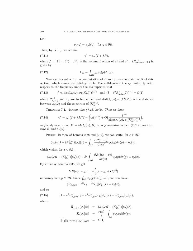
290 7. PLASMONIC RESONANCES FOR NANOPARTICLES
Let
ψp(y) = φp(δy) for y ∈ ∂B.
Then, by (7.10), we obtain
(7.11) γ∗ = εm(I + fP ),
where f = |D| = δ3(= η3β) is the volume fraction of D and P = (Ppq)p,q=1,2,3 isgiven by
(7.12) Ppq =
∫
∂B
yqψp(y)dσ(y).
Now we proceed with the computation of P and prove the main result of thissection, which shows the validity of the Maxwell-Garnett theory uniformly withrespect to the frequency under the assumptions that
(7.13) f ≪ dist(λε(ω), σ((K0B)
∗))3/5 and (I − δ3R−1λε(ω)
T0)−1 = O(1),
where R−1λε(ω)
and T0 are to be defined and dist(λε(ω), σ((K0D)
∗)) is the distance
between λε(ω) and the spectrum of (K0B)
∗.
Theorem 7.4. Assume that (7.13) holds. Then we have
(7.14) γ∗ = εm(I + fM(I − f
3M)−1
)+O
( f8/3
dist(λε(ω), σ((K0B)
∗))2
),
uniformly in ω. Here,M =M(λε(ω), B) is the polarization tensor (2.71) associatedwith B and λε(ω).
Proof. In view of Lemma 2.38 and (7.9), we can write, for x ∈ ∂D,
(λε(ω)I − (K0D)
∗)[φp](x)−∫
∂D
∂R(x− y)
∂ν(x)φp(y)dσ(y) = νp(x),
which yields, for x ∈ ∂B,
(λε(ω)I − (K0B)
∗)[ψp](x)− δ2∫
∂B
∂R(δ(x− y))
∂ν(x)ψp(y)dσ(y) = νp(x).
By virtue of Lemma 2.38, we get
∇R(δ(x− y)) = −δ3(x− y) +O(δ3)
uniformly in x, y ∈ ∂B. Since∫∂B
ψp(y)dσ(y) = 0, we now have
(Rλε(ω) − δ3T0 + δ5T1)[ψp](x) = νp(x),
and so
(7.15) (I − δ3R−1λε(ω)
T0 + δ5R−1λε(ω)
T1)[ψp](x) = R−1λε(ω)
[νp](x),
where
Rλε(ω)[ψp](x) = (λε(ω)I − (K0B)
∗)[ψp](x),
T0[ψp](x) =ν(x)
3·∫
∂B
yψp(y)dσ(y),
‖T1‖L(H∗(∂B),H∗(∂B)) = O(1).
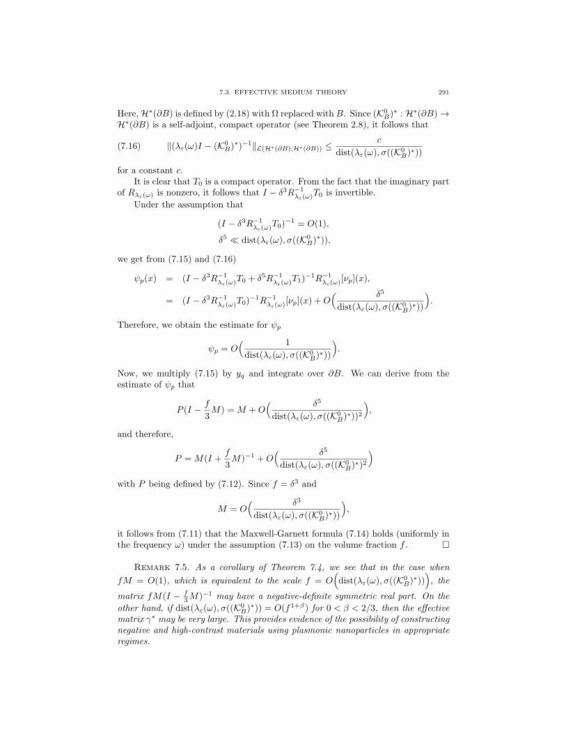
7.3. EFFECTIVE MEDIUM THEORY 291
Here,H∗(∂B) is defined by (2.18) with Ω replaced with B. Since (K0B)
∗ : H∗(∂B) →H∗(∂B) is a self-adjoint, compact operator (see Theorem 2.8), it follows that
(7.16) ‖(λε(ω)I − (K0B)
∗)−1‖L(H∗(∂B),H∗(∂B)) ≤c
dist(λε(ω), σ((K0B)
∗))
for a constant c.It is clear that T0 is a compact operator. From the fact that the imaginary part
of Rλε(ω) is nonzero, it follows that I − δ3R−1λε(ω)
T0 is invertible.
Under the assumption that
(I − δ3R−1λε(ω)
T0)−1 = O(1),
δ5 ≪ dist(λε(ω), σ((K0B)
∗)),
we get from (7.15) and (7.16)
ψp(x) = (I − δ3R−1λε(ω)
T0 + δ5R−1λε(ω)
T1)−1R−1
λε(ω)[νp](x),
= (I − δ3R−1λε(ω)
T0)−1R−1
λε(ω)[νp](x) +O
( δ5
dist(λε(ω), σ((K0B)
∗))
).
Therefore, we obtain the estimate for ψp
ψp = O( 1
dist(λε(ω), σ((K0B)
∗))
).
Now, we multiply (7.15) by yq and integrate over ∂B. We can derive from theestimate of ψp that
P (I − f
3M) =M +O
( δ5
dist(λε(ω), σ((K0B)
∗))2
),
and therefore,
P =M(I +f
3M)−1 +O
( δ5
dist(λε(ω), σ((K0B)
∗)2
)
with P being defined by (7.12). Since f = δ3 and
M = O( δ3
dist(λε(ω), σ((K0B)
∗))
),
it follows from (7.11) that the Maxwell-Garnett formula (7.14) holds (uniformly inthe frequency ω) under the assumption (7.13) on the volume fraction f .
Remark 7.5. As a corollary of Theorem 7.4, we see that in the case when
fM = O(1), which is equivalent to the scale f = O(dist(λε(ω), σ((K0
B)∗))), the
matrix fM(I − f3M)−1 may have a negative-definite symmetric real part. On the
other hand, if dist(λε(ω), σ((K0B)
∗)) = O(f1+β) for 0 < β < 2/3, then the effectivematrix γ∗ may be very large. This provides evidence of the possibility of constructingnegative and high-contrast materials using plasmonic nanoparticles in appropriateregimes.

292 7. PLASMONIC RESONANCES FOR NANOPARTICLES
7.4. Shift in Plasmonic Resonances Due to the Particle Size
In this section we analyze the shift of the plasmon resonance with changes insize of the nanoparticle.
Let MB be defined by (2.311) with D replaced with B and let σj , j = 1, 2, 3, begiven by (2.316). For simplicity we assume that Conditions 2.105 and 2.107 hold.
We consider the original system of integral equations (2.323) for a given incidentplane wave (Ei, Hi). With the same notation as in Section 2.14, the following resultholds by using Lemmas 2.112 and 2.113.
Lemma 7.6. Let η be defined by (7.1). The system of equations (2.323) can berewritten as follows:
WB(δ)
(η(ψ)ωη(φ)
)=
η(ν × Ei)
µm − µcη(√−1ν ×Hi)
εm − εc
∣∣∣∣∣∂B
,(7.17)
where(7.18)
WB(δ) =
λµI −MB + δ2µmMkm
B,2 − µcMkcB,2
µm − µc+O(δ3)
1
µm − µc(δLB,1 + δ2LB,2) +O(δ3)
1
εm − εc(δLB,1 + δ2LB,2) +O(δ3) λεI −MB + δ2
εmMkmB,2 − εcMkc
B,2
εm − εc+O(δ3)
,
and the material parameter contrasts λµ and λε are given by
(7.19) λµ =µc + µm
2(µm − µc), λε =
εc + εm2(εm − εc)
.
It is clear that
WB(0) = WB,0 =
(λµI −MB 0
0 λεI −MB
).
Moreover,
WB(δ) = WB,0 + δWB,1 + δ2WB,2 +O(δ3),
in the sense that
‖WB(δ)−WB,0 − δWB,1 − δ2WB,2‖ ≤ Cδ3
for a constant C independent of δ. Here ‖A‖ = supi,j ‖Ai,j‖H
− 12
T (div,∂B)for any
operator-valued matrix A with entries Ai,j .
We are now interested in finding W−1B (δ). The following result holds.
Lemma 7.7. The system of equations (2.323) is equivalent to
WB(δ)
η(ψ)(1)
η(ψ)(2)
ωη(φ)(1)
ωη(φ)(2)
=
η(ν × Ei)(1)
µm − µcη(ν × Ei)(2)
µm − µcη(√−1ν ×Hi)(1)
εm − εcη(√−1ν ×Hi)(2)
εm − εc
∣∣∣∣∣∂B
,(7.20)
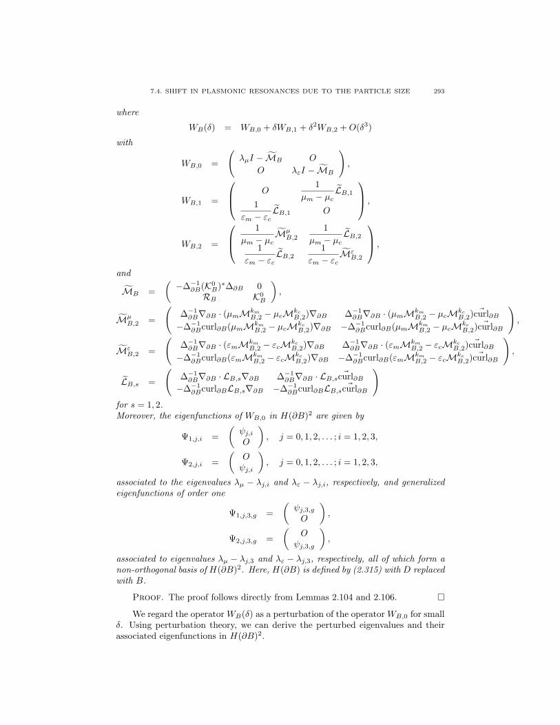
7.4. SHIFT IN PLASMONIC RESONANCES DUE TO THE PARTICLE SIZE 293
where
WB(δ) = WB,0 + δWB,1 + δ2WB,2 +O(δ3)
with
WB,0 =
(λµI − MB O
O λεI − MB
),
WB,1 =
O1
µm − µcLB,1
1
εm − εcLB,1 O
,
WB,2 =
1
µm − µcMµ
B,2
1
µm − µcLB,2
1
εm − εcLB,2
1
εm − εcMε
B,2
,
and
MB =
(−∆−1
∂B(K0B)
∗∆∂B 0RB K0
B
),
MµB,2 =
(∆−1∂B∇∂B · (µmMkm
B,2 − µcMkcB,2)∇∂B ∆−1
∂B∇∂B · (µmMkmB,2 − µcMkc
B,2)~curl∂B
−∆−1∂Bcurl∂B(µmMkm
B,2 − µcMkcB,2)∇∂B −∆−1
∂Bcurl∂B(µmMkmB,2 − µcMkc
B,2)~curl∂B
),
MεB,2 =
(∆−1∂B∇∂B · (εmMkm
B,2 − εcMkcB,2)∇∂B ∆−1
∂B∇∂B · (εmMkmB,2 − εcMkc
B,2)~curl∂B
−∆−1∂Bcurl∂B(εmMkm
B,2 − εcMkcB,2)∇∂B −∆−1
∂Bcurl∂B(εmMkmB,2 − εcMkc
B,2)~curl∂B
),
LB,s =
(∆−1∂B∇∂B · LB,s∇∂B ∆−1
∂B∇∂B · LB,s ~curl∂B−∆−1
∂Bcurl∂BLB,s∇∂B −∆−1∂Bcurl∂BLB,s ~curl∂B
)
for s = 1, 2.Moreover, the eigenfunctions of WB,0 in H(∂B)2 are given by
Ψ1,j,i =
(ψj,iO
), j = 0, 1, 2, . . . ; i = 1, 2, 3,
Ψ2,j,i =
(Oψj,i
), j = 0, 1, 2, . . . ; i = 1, 2, 3,
associated to the eigenvalues λµ − λj,i and λε − λj,i, respectively, and generalizedeigenfunctions of order one
Ψ1,j,3,g =
(ψj,3,gO
),
Ψ2,j,3,g =
(O
ψj,3,g
),
associated to eigenvalues λµ − λj,3 and λε − λj,3, respectively, all of which form anon-orthogonal basis of H(∂B)2. Here, H(∂B) is defined by (2.315) with D replacedwith B.
Proof. The proof follows directly from Lemmas 2.104 and 2.106.
We regard the operatorWB(δ) as a perturbation of the operatorWB,0 for smallδ. Using perturbation theory, we can derive the perturbed eigenvalues and theirassociated eigenfunctions in H(∂B)2.

294 7. PLASMONIC RESONANCES FOR NANOPARTICLES
We denote by Γ =(k, j, i) : k = 1, 2; j = 1, 2, . . . ; i = 1, 2, 3
the set of indices
for the eigenfunctions of WB,0 and by Γg =(k, j, 3, g) : k = 1, 2; j = 1, 2, . . .
the
set of indices for the generalized eigenfunctions. We denote by γg the generalizedeigenfunction index corresponding to eigenfunction index γ and vice-versa. We alsodenote by
(7.21) τγ =
λµ − λj,i, k = 1,λε − λj,i, k = 2.
Condition 7.8. λµ 6= λε.
In the following we will only consider γ ∈ Γ for which there is no generalizedeigenfunction index associated. In other words, we only consider γ = (k, i, j) ∈ Γsuch that λj,i ∈ σ1 ∪ σ2 (see (2.316) for the definitons). We call this subset Γsim.Note that Conditions 2.105 and 7.8 imply that the eigenvalues of WB,0 indexed byγ ∈ Γsim are simple.
Theorem 7.9. As δ → 0, the perturbed eigenvalues and eigenfunctions indexedby γ ∈ Γsim have the following asymptotic expansions:
τγ(δ) = τγ + δτγ,1 + δ2τγ,2 +O(δ3),(7.22)
Ψγ(δ) = Ψγ + δΨγ,1 +O(δ2),
where
τγ,1 =〈WB,1Ψγ , Ψγ〉H(∂B)2
〈Ψγ , Ψγ〉H(∂B)2= 0,
τγ,2 =〈WB,2Ψγ , Ψγ〉H(∂B)2 − 〈WB,1Ψγ,1, Ψγ〉H(∂B)2
〈Ψγ , Ψγ〉H(∂B)2,(7.23)
(τγ −WB,0)Ψγ,1 = −WB,1Ψγ .
Here, Ψγ′ ∈ Ker(τγ′ −W ∗B,0) and W
∗B,0 is the H(∂B)2 adjoint of WB,0.
Using Lemma 2.109 and Remark 2.111 we can solve Ψγ,1. Indeed,
Ψγ,1 =∑
γ′∈Γγ′ 6=γ
α(−WB,1Ψγ ,Ψγ′)Ψγ′
τγ − τγ′+∑
γ′g∈Γg
γ′ 6=γ
α(−WB,1Ψγ ,Ψγ′g)
(Ψγ′
g
τγ − τγ′+
Ψγ′
(τγ − τγ′)2
)
+ α(−WB,1Ψγ ,Ψγ)Ψγ .
By abuse of notation,
α(x,Ψγ) =
α(x1, ψκ) γ = (1, j, i), κ = (j, i),α(x2, ψκ) γ = (2, j, i), κ = (j, i),
(7.24)
for
x =
(x1x2
)∈ H(∂B)2
with α being introduced in Definition 2.108.
Consider now the degenerate case γ ∈ Γ\Γsim =: Γdeg = γ = (k, i, j) ∈ Γs.t λj,i ∈ σ3. It is clear that, for γ ∈ Γdeg, the algebraic multiplicity of theeigenvalue τγ is 2 while the geometric multiplicity is 1. In this case every eigenvalue

7.4. SHIFT IN PLASMONIC RESONANCES DUE TO THE PARTICLE SIZE 295
τγ and associated eigenfunction Ψγ will split into two branches, as δ goes to zero,represented by a convergent Puiseux series as
τγ,h(δ) = τγ + (−1)hδ1/2τγ,1 + (−1)2hδ2/2τγ,2 +O(δ3/2), h = 0, 1,(7.25)
Ψγ,h(δ) = Ψγ + (−1)hδ1/2Ψγ,1 + (−1)2hδ2/2Ψγ,2 +O(δ3/2), h = 0, 1,
where τγ,j and Ψγ,j can be recovered by recurrence formulas; see Section 2.9.6.Recall that the electric and magnetic parameters, εc and µc, depend on the
frequency of the incident field, ω, following a Drude model. Therefore, the eigen-values of the operator WB,0 and the perturbation in the eigenvalues depend on thefrequency as well, that is,
τγ(δ, ω) = τγ(ω) + δ2τγ,2(ω) +O(δ3), γ ∈ Γsim,
τγ,h(δ, ω) = τγ + δ1/2(−1)hτγ,1(ω) + δ2/2(−1)2hτγ,2(ω) +O(δ3/2), γ ∈ Γdeg, h = 0, 1.
In the sequel, we will omit frequency dependence to simplify the notation. However,we will keep in mind that all these quantities are frequency dependent.
We first state the following result.
Proposition 7.10. If ω is a quasi-static plasmonic resonance (as stated inDefinition 7.2), then |τγ | ≪ 1 and is locally minimized for some γ ∈ Γ with τγbeing defined by (7.21).
Then we recall two different notions of plasmonic resonance [71].
Definition 7.11. (i) We say that ω is a plasmonic resonance if |τγ(δ)| ≪1 and is locally minimized for some γ ∈ Γsim or |τγ,h(δ)| ≪ 1 and is locallyminimized for some γ ∈ Γdeg, h = 0, 1.
(ii) We say that ω is a first-order corrected quasi-static plasmonic resonanceif |τγ + δ2τγ,2| ≪ 1 and is locally minimized for some γ ∈ Γsim or |τγ +
δ1/2(−1)hτγ,1| ≪ 1 and is locally minimized for some γ ∈ Γdeg, h = 0, 1.Here, the correction terms τγ,2 and τγ,1 are defined by (7.23) and (7.25).
Note that quasi-static resonance is size independent and is therefore a zero-order approximation of the plasmonic resonance in terms of the particle size whilethe first-order corrected quasi-static plasmonic resonance depends on the size of thenanoparticle.
We are interested in solving equation (7.20)
WB(δ)[Ψ] = f,
where
Ψ =
η(ψ)(1)
η(ψ)(2)
ωη(φ)(1)
ωη(φ)(2)
, f =
η(ν × Ei)(1)
µm − µcη(ν × Ei)(2)
µm − µcη(√−1ν ×Hi)(1)
εm − εcη(√−1ν ×Hi)(2)
εm − εc
∣∣∣∣∣∂B
for ω close to the resonance frequencies, i.e., when τγ(δ) is very small for someγ’s ∈ Γsim or τγ,h(δ) is very small for some γ’s ∈ Γdeg, h = 0, 1. In this case,
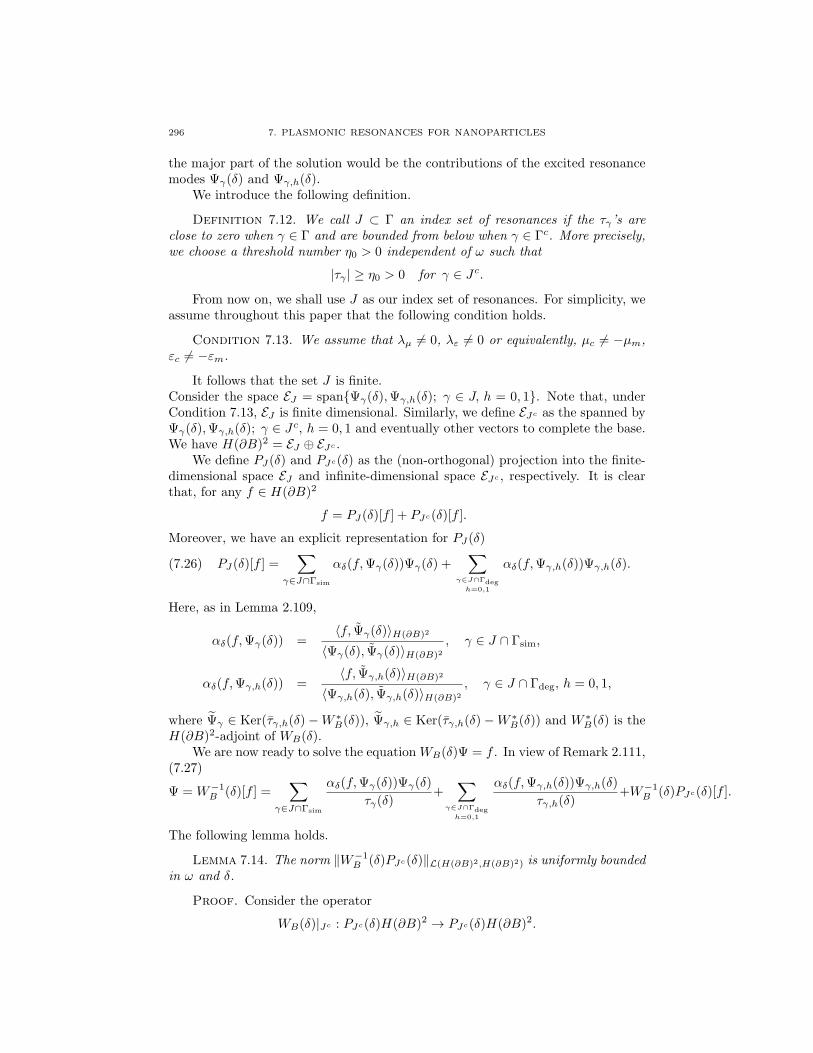
296 7. PLASMONIC RESONANCES FOR NANOPARTICLES
the major part of the solution would be the contributions of the excited resonancemodes Ψγ(δ) and Ψγ,h(δ).
We introduce the following definition.
Definition 7.12. We call J ⊂ Γ an index set of resonances if the τγ ’s areclose to zero when γ ∈ Γ and are bounded from below when γ ∈ Γc. More precisely,we choose a threshold number η0 > 0 independent of ω such that
|τγ | ≥ η0 > 0 for γ ∈ Jc.
From now on, we shall use J as our index set of resonances. For simplicity, weassume throughout this paper that the following condition holds.
Condition 7.13. We assume that λµ 6= 0, λε 6= 0 or equivalently, µc 6= −µm,εc 6= −εm.
It follows that the set J is finite.Consider the space EJ = spanΨγ(δ),Ψγ,h(δ); γ ∈ J, h = 0, 1. Note that, underCondition 7.13, EJ is finite dimensional. Similarly, we define EJc as the spanned byΨγ(δ),Ψγ,h(δ); γ ∈ Jc, h = 0, 1 and eventually other vectors to complete the base.We have H(∂B)2 = EJ ⊕ EJc .
We define PJ(δ) and PJc(δ) as the (non-orthogonal) projection into the finite-dimensional space EJ and infinite-dimensional space EJc , respectively. It is clearthat, for any f ∈ H(∂B)2
f = PJ(δ)[f ] + PJc(δ)[f ].
Moreover, we have an explicit representation for PJ(δ)
(7.26) PJ(δ)[f ] =∑
γ∈J∩Γsim
αδ(f,Ψγ(δ))Ψγ(δ) +∑
γ∈J∩Γdegh=0,1
αδ(f,Ψγ,h(δ))Ψγ,h(δ).
Here, as in Lemma 2.109,
αδ(f,Ψγ(δ)) =〈f, Ψγ(δ)〉H(∂B)2
〈Ψγ(δ), Ψγ(δ)〉H(∂B)2, γ ∈ J ∩ Γsim,
αδ(f,Ψγ,h(δ)) =〈f, Ψγ,h(δ)〉H(∂B)2
〈Ψγ,h(δ), Ψγ,h(δ)〉H(∂B)2, γ ∈ J ∩ Γdeg, h = 0, 1,
where Ψγ ∈ Ker(τγ,h(δ)−W ∗B(δ)), Ψγ,h ∈ Ker(τγ,h(δ)−W ∗
B(δ)) and W∗B(δ) is the
H(∂B)2-adjoint of WB(δ).We are now ready to solve the equationWB(δ)Ψ = f . In view of Remark 2.111,
(7.27)
Ψ =W−1B (δ)[f ] =
∑
γ∈J∩Γsim
αδ(f,Ψγ(δ))Ψγ(δ)
τγ(δ)+
∑
γ∈J∩Γdegh=0,1
αδ(f,Ψγ,h(δ))Ψγ,h(δ)
τγ,h(δ)+W−1
B (δ)PJc(δ)[f ].
The following lemma holds.
Lemma 7.14. The norm ‖W−1B (δ)PJc(δ)‖L(H(∂B)2,H(∂B)2) is uniformly bounded
in ω and δ.
Proof. Consider the operator
WB(δ)|Jc : PJc(δ)H(∂B)2 → PJc(δ)H(∂B)2.

7.4. SHIFT IN PLASMONIC RESONANCES DUE TO THE PARTICLE SIZE 297
We can show that for every ω and δ, dist(σ(WB(δ)|Jc), 0) ≥ η02 , where σ(WB(δ)|Jc)
is the discrete spectrum of WB(δ)|Jc . Here and throughout the paper, dist denotesthe distance. Then, it follows that
‖W−1B (δ)PJc(δ)[f ]‖ = ‖W−1
B (δ)|JcPJc(δ)[f ]‖ .1
η0exp(
C1
η20)‖PJc(δ)[f ]‖ .
1
η0exp(
C1
η20)‖f‖,
where the notation A . B means that A ≤ CB for some constant C independentof A and B.
Finally, we are ready to state our main result in this section.
Theorem 7.15. Let η be defined by (7.1). Under Conditions 2.105, 2.107, 7.8and 7.13, the scattered field Es = E−Ei due to a single plasmonic particle has thefollowing representation:
Es = µm∇× ~SkmD [ψ](x) +∇×∇× ~SkmD [φ](x) x ∈ R3\D,
where
ψ = η−1(∇∂Bψ
(1) + ~curl∂Bψ(2)),
φ =1
ωη−1
(∇∂Bφ
(1) + ~curl∂Bφ(2)),
Ψ =
ψ(1)
ψ(2)
φ(1)
φ(2)
=
∑
γ∈J∩Γsim
α(f,Ψγ)Ψγ +O(δ)
τγ(δ)+
∑
γ∈J∩Γdeg
ζ1(f)Ψγ + ζ2(f)Ψγ,1 +O(δ1/2)
τγ,0(δ)τγ,1(δ)+O(1),
and
ζ1(f) =〈f, Ψγ,1〉H(∂B)2τγ − 〈f, Ψγ〉H(∂B)2(τγ,1 + τγ
a2a1)
a1,
ζ2(f) =〈f, Ψγ〉H(∂B)2
a1,
a1 = 〈Ψγ , Ψγ,1〉H(∂B)2 + 〈Ψγ,1, Ψγ〉H(∂B)2 ,
a2 = 〈Ψγ , Ψγ,2〉H(∂B)2 + 〈Ψγ,2, Ψγ〉H(∂B)2 + 〈Ψγ,1, Ψγ,1〉H(∂B)2 .
Proof. Recall that
Ψ =∑
γ∈J∩Γsim
αδ(f,Ψγ(δ))Ψγ(δ)
τγ(δ)+
∑
γ∈J∩Γdegh=0,1
αδ(f,Ψγ,h(δ))Ψγ,h(δ)
τγ,h(δ)+W−1
B (δ)PJc(δ)[f ].
By Lemma 7.14, we have W−1B (δ)PJc(δ)[f ] = O(1).
If γ ∈ J ∩ Γsim, an asymptotic expansion on δ yields
αδ(f,Ψγ(δ))Ψγ(δ) = α(f,Ψγ)Ψγ +O(δ).

298 7. PLASMONIC RESONANCES FOR NANOPARTICLES
If γ ∈ J ∩ Γdeg then 〈Ψγ , Ψγ〉H(∂B)2 = 0. Therefore, an asymptotic expansion on δyields
αδ(f,Ψγ,h(δ))Ψγ,h(δ) =(−1)h〈f, Ψγ〉H(∂B)2Ψγ
δ−1/2a1+
1
a1
((〈f, Ψγ,1〉H(∂B)2 − 〈f, Ψγ〉H(∂B)2
a2a1
)Ψγ + 〈f, Ψγ〉H(∂B)2Ψγ,1
)
+O(δ1/2)
with
a1 = 〈Ψγ , Ψγ,1〉H(∂B)2 + 〈Ψγ,1, Ψγ〉H(∂B)2 ,
a2 = 〈Ψγ , Ψγ,2〉H(∂B)2 + 〈Ψγ,2, Ψγ〉H(∂B)2 + 〈Ψγ,1, Ψγ,1〉H(∂B)2 .
Since τγ,h(δ) = τγ + δ1/2(−1)hτγ,1 +O(δ), the result follows by adding the terms
αδ(f,Ψγ,0(δ))Ψγ,0(δ)
τγ,0(δ)and
αδ(f,Ψγ,1(δ))Ψγ,1(δ)
τγ,1(δ).
The proof is then complete.
Corollary 7.16. Assume the same conditions as in Theorem 7.15. Under theadditional condition that
(7.28) minγ∈J∩Γsim
|τγ(δ)| ≫ δ3, minγ∈J∩Γdeg
|τγ(δ)| ≫ δ,
we have
Ψ =∑
γ∈J∩Γsim
α(f,Ψγ)Ψγ +O(δ)
τγ + δ2τγ,2+
∑
γ∈J∩Γdeg
ζ1(f)Ψγ + ζ2(f)Ψγ,1 +O(δ1/2)
τ2γ − δτ2γ,1+O(1).
Corollary 7.17. Assume the same conditions as in Theorem 7.15. Under theadditional condition that
(7.29) minγ∈J∩Γsim
|τγ(δ)| ≫ δ2, minγ∈J∩Γdeg
|τγ(δ)| ≫ δ1/2,
we have
Ψ =∑
γ∈J∩Γsim
α(f,Ψγ)Ψγ +O(δ)
τγ+
∑
γ∈J∩Γdeg
α(f,Ψγ)Ψγτγ
+ α(f,Ψγ,g)
(Ψγ,gτγ
+Ψγτ2γ
)+O(1).
Proof. We have
limδ→0
W−1B (δ)PspanΨγ,0(δ),Ψγ,1(δ)[f ] = lim
δ→0
αδ(f,Ψγ,0(δ))Ψγ,0(δ)
τγ,0(δ)+αδ(f,Ψγ,1(δ))Ψγ,1(δ)
τγ,1(δ)
= W−1B,0(δ)PspanΨγ ,Ψγg[f ]
=α(f,Ψγ)Ψγ
τγ+ α(f,Ψγ,g)
(Ψγ,gτγ
+Ψγτ2γ
),
where γ ∈ J ∩ Γdeg, f ∈ H(∂B)2 and PspanE is the projection into the linear spacegenerated by the elements in the set E.
Remark 7.18. Note that for γ ∈ J ,
τγ ≈ mindist
(λµ, σ((K0
B)∗) ∪ −σ((K0
B)∗)), dist
(λε, σ((K0
B)∗) ∪ −σ((K0
B)∗)).

7.4. SHIFT IN PLASMONIC RESONANCES DUE TO THE PARTICLE SIZE 299
It is clear, from Remark 7.18, that resonances can occur when exciting thespectrum of (K0
B)∗ or/and that of −(K0
B)∗. We substantiate in the following that
only the spectrum of (K0B)
∗ can be excited to create the plasmonic resonances inthe quasi-static regime.Recall that
f =
η(ν × Ei)(1)
µm − µcη(ν × Ei)(2)
µm − µcη(√−1ν ×Hi)(1)
εm − εcη(√−1ν ×Hi)(2)
εm − εc
∣∣∣∣∣∂B
,
and therefore,
f1 :=η(ν × Ei)(1)
µm − µc=
∆−1∂B∇∂B · η(ν × Ei)
µm − µc.
Now, suppose γ = (1, j, 1) ∈ J (recall that J is the index set of resonances). Thenτγ = λµ − λ1,j , where λ1,j ∈ σ1 = σ(−(K0
B)∗)\σ((K0
B)∗). From Remark 2.110,
α(f,Ψγ) = 〈∆∂Bf1, ϕj,1〉H∗ = α(f,Ψγ) =1
µm − µc〈∇∂B · η(ν × Ei), ϕj,1〉H∗ ,
where ϕj,1 ∈ H∗0(∂B) is a normalized eigenfunction of (K0
B)∗(∂B).
A Taylor expansion of Ei gives, for x ∈ ∂D,
Ei(x) =∞∑
β∈N3
(x− z)β∂βEi(z)
|β|! .
Thus,
η(ν × Ei)(x) = η(ν)(x)× Ei(z) +O(δ),
and
∇∂B · η(ν × Ei)(x) = −η(ν)(x) · ∇ × Ei(z) +O(δ)
= O(δ).
Therefore, the zeroth-order term of the expansion of ∇∂B · η(ν × Ei) in δ is zero.Hence,
α(f,Ψγ) = 0.
In the same way, we have
α(f,Ψγ) = 0,
α(f,Ψγg ) = 0
for γ = (2, j, 1) ∈ J and γg such that γ ∈ J .As a result we see that the spectrum of−(K0
B)∗ is not excited in the zeroth-order
term. However, we note that σ(−(K0B)
∗) can be excited in higher-order terms.Finally, we sketch a proof of Theorem 7.1. From (2.321), we have
Es(x) = µm∇× ~SkmD [ψ](x) +∇×∇× ~SkmD [φ](x), x ∈ R3 \D,

300 7. PLASMONIC RESONANCES FOR NANOPARTICLES
where ψ and φ are determined by (7.17). Since WB(δ) = WB,0 + O(δ), formula(7.2) follows by using the identities stated in Lemma 2.102.
7.4.1. Numerical Examples. Here we present numerical examples to demon-strate the shift of the plasmonic resonance. The first example involves a sphericalnanoparticle of radius R with permittivity ǫc. For the permittivity ǫc, we useDrude’s model as follows: ǫc(ω) = 1 − ω2
p/(ω(ω +√−1γ)) where ωp = 5.8(eV )
and γ = 0.2. We compute the extinction cross-section Qext as a function of theoperating wavelength λ = 2πc/ω. Due to spherical symmetry, it can be shown thatQext has the following simple representation
Qext =2
(kmR)2
∞∑
n=1
(2n+ 1)ℜ √
−1kmn(n+ 1)
(WTEn +WTM
n ),
where WTEn and WTM
n are the scattering coefficients of a spherical structure. Wehave already seen in section 2.14 how to computeWTE
n andWTMn using Code Scat-
tering Coefficients for Maxwell’s Equations . We use Code Plasmonic ResonanceShift to repeatedly plot Qext while changing the radius R from 5 nm to 30 nm inFigure 7.2. The shift of the plasmonic resonance is clearly shown.
We also present numerical example of a spherical shell with outer radius R andinner radius R/2. We also assume the outer sphere has the permittivity ǫc and theinner sphere has the same permittivity as background. In Figure 7.2, we plot Qext
for the shell for various values of radius R. Again, the shift of plasmon resonanceis clearly shown.
7.5. Plasmonic Resonance for a System of Spheres
Confining light at the nanoscale is challenging due to the diffraction limit.Strongly localized surface plasmon modes in singular metallic structures, such assharp tips and two nearly touching surfaces, offer a promising route to overcomethis difficulty. Recently, transformation optics has been applied to analyze variousstructural singularities and then provides novel physical insights for a broadbandnanofocusing of light.
Among three-dimensional singular structures, the system of nearly touchingspheres is of fundamental importance. In the narrow gap regions, a large field en-hancement occurs. The significant spectral shift of resonance mode also occurs dueto the plasmon hybridization. A cluster of plasmonic spheres such as a heptamerand a octamer can support collective resonance modes such as Fano resonances. Fortheoretical investigations of these phenomena, the numerical computation plays aimportant role. Unfortunately, in the nearly touching case, it is quite challeng-ing to compute the field distribution in the gap accurately. In fact, the requiredcomputational cost dramatically increases as the spheres get closer. The multipoleexpansion method requires a large number of spherical harmonics and the finiteelement method (or boundary element method) requires very fine mesh in the gap.Moreover, the linear systems to be solved are ill-conditioned. So conventional nu-merical methods are time consuming or inaccurate for this extreme case.
Here we present a hybrid numerical scheme that overcomes difficulty. Thekey idea of our hybrid scheme is to clarify the connection between TransformationOptics and the image charge method. The developed code is Code PlasmonicResonance for Nearly Touching Spheres. The results of this section are from [465].
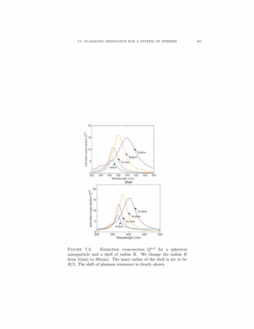
7.5. PLASMONIC RESONANCE FOR A SYSTEM OF SPHERES 301
Wavelength (nm)300 350 400 450 500
extin
ctio
n c
ross s
ectio
n Q
ext
0
5
10
15
20
Shell
R=10nm
R=20nm
R=30nm
R=5nm
Figure 7.2. Extinction cross-section Qext for a sphericalnanoparticle and a shell of radius R. We change the radius Rfrom 5(nm) to 30(nm). The inner radius of the shell is set to beR/2. The shift of plasmon resonance is clearly shown.

302 7. PLASMONIC RESONANCES FOR NANOPARTICLES
7.5.1. Two Metallic Spheres. We consider the two metallic spheres whichare shown in Figure 7.3. The permittivity ǫ of each individual sphere is modeledas ǫ = 1−ω2
p/(ω(ω+√−1γ)) where ω is the operating frequency, ωp is the plasma
frequency and γ is the damping parameter. We fit Palik’s data [394] for silverby adding a few Lorentz terms. We shall assume that the plasmonic spheres aresmall compared to optical wavelengths so that the quasi-static approximation canbe adopted.
a
x y
z
ε0 = 1B
−
ε
δ 2d
B+
R
b
ε0 = R2
T |r0 −R00|ε
R0
R00
R00δ0
Figure 7.3. Two spheres and the transformation optics inversionmapping. (a) Two identical spheres, each of radius R and per-mittivity ǫ, are separated by a distance δ. The distance betweentheir centers is 2d. The background permittivity is ǫ0 = 1. (b)The transformation optics inversion mapping transforms the lowersphere B− (or the upper sphere B+) into a sphere of radius R′ (ora hollow sphere of radius R′′) centered at the origin, respectively.
7.5.2. Transformation Optics. Let us briefly review the transformation op-tics approach by Pendry et al. [401]. To transform two spheres into a concentricshell, Pendry et al. introduced the inversion transformation Φ defined as
(7.30) x′ = Φ(x) = R2T (x−X0)/|x−X0|2 +X ′
0
where X0, X′0 and RT are given parameters. This inversion mapping induces the
inhomogeneous permittivity ǫ′(x′) = R2T |x′−X ′
0|ǫ in the transformed space. Then,by taking advantage of the symmetry of the shell, the electric potential can berepresented in terms of the following basis functions:
(7.31) Mmn,±(x) = |x′ −X ′
0|(r′)±(n+ 12 )− 1
2Y mn (θ′, φ′),
where Y mn are the spherical harmonics and (r′, θ′, φ′) are the spherical coordi-nates. We will call Mm
n,± a transformation optics basis.Let us assume that two plasmonic spheres B+ ∪ B− are placed in a uniform
incident field (0, 0, E0ℜe√−1ωt). Then the (quasi-static) electrical potential V
outside the two spheres can be represented in the following form:
(7.32) V (x) = −E0x3 +
∞∑
n=0
An(M0
n,+(x)−M0n,−(x)
)

7.5. PLASMONIC RESONANCE FOR A SYSTEM OF SPHERES 303
Here, the coefficients An can be determined by solving some tridiagonal systemand x1, x2, x3 are the Cartesian coordinates. Unfortunately, it cannot be solvedanalytically.
R(0,0,‐zk)
‐u0 ‐u1 ‐u2
x
u2 u1 u0
(0,0,+zk)
zR
……
B+B‐
Figure 7.4. Image charges for two spheres. Red and green circlesrepresent image charges placed along the x3-axis.
7.5.3. Method of Image Charges. Now we discuss the method of images.Since the imaging rule for a pair of cylinders is simple, an exact image series solu-tion and its properties can be easily derived. However, for two dielectric spheres, anexact solution cannot be obtained due to the appearance of a continuous line imagesource. Poladian observed in [406] that the continuous source can be well approxi-mated by a point charge and then derived an approximate but analytic image seriessolution. Let us briefly review Poladian’s solution for two dielectric spheres. Letτ = (ǫ− 1)/(ǫ+ 1), s = cosh−1(d/R) and α = R sinh s. Suppose that two pointcharges of strength ±1 are located at (0, 0,±z0) ∈ B±, respectively. By Poladian’simaging rule, they produce an infinite series of image charges of strength ±uk at(0, 0,±zk) for k = 0, 1, 2, . . ., where zk and uk are given by
(7.33) zk = α coth(ks+ s+ t0), uk = τksinh(s+ t0)
sinh(ks+ s+ t0).
Here, the parameter t0 is such that z0 = α coth(s + t0). See Figure 7.4. Thepotential U(x) generated by all the above image charges is given by
(7.34) U(x) =
∞∑
k=0
uk(Γ0(x− xk)− Γ0(x+ xk))
where xk = (0, 0, zk) and Γ0(x) = 1/(4π|x|).Let us consider the potential V outside the two spheres when a uniform incident
field (0, 0, E0ℜe√−1ωt) is applied. Let p0 be the induced polarizability when a sin-
gle sphere is subjected to the uniform incident field, that is, p0 = E0R32τ/(3− τ).
Using the potential U(x), we can derive an approximate solution for V (x). For|τ | ≈ 1, we have
(7.35) V (x) ≈ −E0x3 + 4πp0∂(U(x))
∂z0
∣∣∣z0=d
+QU(x)|z0=d,
where Q is a constant chosen so that the right-hand side in equation (7.35) has nonet flux on the surface of each sphere. The accuracy of the approximate formula,

304 7. PLASMONIC RESONANCES FOR NANOPARTICLES
equation (7.35), improves as |ǫ| increases and it becomes exact when |ǫ| = ∞.Moreover, its accuracy is pretty good even if the value of |ǫ| is moderate.
We now explain the difficulty involved in applying the the image series solution,equation (7.35), to the case of plasmonic spheres. In view of the expressions for uk,equation (7.33), we can see that equation (7.35) is not convergent when |τ | > es.For plasmonic materials such as gold and silver, the real part of the permittivityǫ is negative over the optical frequencies and this means that the correspondingparameter |τ | can attain any value in the interval (es,∞). Moreover, it turns outthat all the plasmonic resonant values for τ are contained in the set τ ∈ C : |τ | >es. So, equation (7.35) cannot describe the plasmonic interaction between thespheres due to the non-convergence.
7.5.4. Analytical Solution for Two Plasmonic Spheres. Here we presentan analytic approximate solution for two plasmonic spheres in a uniform incident
field (0, 0, E0ℜe√−1ωt). More importantly, we shall see that our analytical ap-
proximation completely captures the singular behavior of the exact solution. Thisfeature is essential in developing our hybrid numerical scheme.
The solution which is valid for two plasmonic spheres can be derived by es-tablishing the explicit connection between transformation optics and the methodof image charges. We can convert the image series into a transformation optics-type solution by using the explicit connection formula. The result is shown in thefollowing theorem.
Theorem 7.19. If |τ | ≈ 1, the following approximation for the electric potentialV (x) holds: for x ∈ R3 \ (B+ ∪B−),
(7.36) V (x) ≈ −E0x3 +
∞∑
n=0
An
(M0
n,+(x)−M0n,−(x)
),
where the coefficient An is given by
(7.37)
An = E02τα
3− τ· 2n+ 1− γ0e(2n+1)s − τ
,
γ0 =
∞∑
n=0
2n+ 1
e(2n+1)s − τ
/ ∞∑
n=0
1
e(2n+1)s − τ.
As expected, the above approximate expression is valid even if |τ | > es. There-fore, it can furnish useful information about the plasmonic interaction between thetwo spheres. As a first demonstration, let us investigate the (approximate) reso-
nance condition, that is, the condition for τ at which the coefficients An diverge.One might conclude that the resonance condition is given by τ = e(2n+1)s. How-
ever, one can see that An has a removable singularity at each τ = e(2n+1)s. In fact,the (approximate) resonance condition turns out to be
(7.38)∞∑
n=0
1
e(2n+1)s − τ= 0.
In other words, the plasmonic resonance happens when τ is one of the zeros ofequation (7.38). It turns out that the zeros τn∞n=0 lie on the positive real axisand satisfy, for n = 0, 1, 2, . . .,
(7.39) e(2n+1)s < τn < e(2n+3)s.

7.5. PLASMONIC RESONANCE FOR A SYSTEM OF SPHERES 305
Frequency (eV)0.5 1 1.5 2 2.5 3 3.5 4
|E/E
0|
100
102
104
106
Field enhancement
approx. exact
δ=10
δ=1
δ=0.1
δ=0.01
δ=0.001
a
Frequency (eV)0.5 1 1.5 2 2.5 3 3.5 4
σa/4π
R3
10-5
10-4
10-3
10-2
10-1
100
101Absorption cross sectionb
approx. exact
δ=10
δ=1
δ=0.1δ=0.01
δ=0.001
Figure 7.5. Exact solution vs Analytic approximation. (a) Fieldenhancement plot as a function of frequency ω for various separa-tion distances δ. The solid lines represent the approximate ana-lytical solution and the dashed lines represent the exact solution.Two identical silver spheres of radius 30 nm are considered. (b)Same as (a) but for the absorption cross section.
The above estimate helps us understand the asymptotic behavior of the resonancewhen two spheres get closer. As the separation distance δ goes to zero, the param-eter s also goes to zero (in fact, s = O(δ1/2)). Then, in view of equation (7.39),τn will converge to 1 and the corresponding permittivity ǫn goes to infinity. Thismeans that a red-shift of the (bright) resonance modes occurs. Since the approxi-mate analytical formula for V becomes more accurate as |ǫ| increases, we can expectthat accuracy improves as the separation distance goes to zero. It also indicatesthat our formula captures the singular nature of the field distribution completely.Furthermore, the difference between τn and τn+1 decreases, which means that thespectrum becomes almost continuous.
We now derive approximate formulas for the field at the gap and for the ab-sorption cross section. From Theorem 7.19, we obtain the following:
(7.40)
E(0, 0, 0) ≈ E0 − E08τ
3− τ
[ ∞∑
n=0
(2n+ 1)2
e(2n+1)s − τ(−1)n
−γ0∞∑
n=0
2n+ 1
e(2n+1)s − τ(−1)n
].
In the quasi-static approximation, the absorption cross section σa is definedby σa = ωℑp, where p is the polarizability of the system of two spheres. FromTheorem 7.19, σa is approximated as follows:
(7.41)
σa ≈ ωE08τα3
3− τ
[ ∞∑
n=0
(2n+ 1)2
e(2n+1)s − τ
−( ∞∑
n=0
2n+ 1
e(2n+1)s − τ
)2/ ∞∑
n=0
1
e(2n+1)s − τ
] .
We compare the above approximate formulas with the exact ones. Figure 7.5represents respectively the field enhancement and the absorption cross section σa asfunctions of the frequency ω for various distances ranging from 0.001 nm to 10 nm.

306 7. PLASMONIC RESONANCES FOR NANOPARTICLES
The strong accuracy of our approximate formulas over broad ranges of frequenciesand gap distances is clearly shown. As mentioned previously, the accuracy improvesas the spheres get closer. It is also worth highlighting the red-shift of the plasmonicresonance modes as the separation distance δ goes to zero.
β
R
δ
δ
A
B3
B2B1
z
a
Frequency(eV)1.5 2 2.5 3
Fie
ld e
nh
an
ce
me
nt
0
500
1000
1500
2000
2500
3000
3500Multipole expansion methodb
L=20L=30L=50exact
Frequency(eV)1.5 2 2.5 3
Fie
ld e
nh
an
ce
me
nt
0
500
1000
1500
2000
2500
3000
3500Hybrid methodc
L=2L=5L=20exact
δ
R
δ
δ
B3
B2B1
A
z
d
Frequency(eV)1.5 2 2.5 3
Fie
ld e
nh
an
ce
me
nt
0
500
1000
1500
2000
2500
3000
3500
Multipole expansion methode
L=20L=30L=50exact
Frequency(eV)1.5 2 2.5 3
Fie
ld e
nh
an
ce
me
nt
0
500
1000
1500
2000
2500
3000
3500
Hybrid methodf
L=2L=5L=20exact
Figure 7.6. Multipole expansion method versus Hybrid scheme.(a) and (d) Two examples of three spheres configuration. (b) and(c) The field enhancement at point A as a function of frequencyfor the configuration (a) using the multipole expansion methodand the hybrid method, respectively. The parameters are given asR = 30 nm, δ = 0.25 nm and β = 80. The uniform incident field
(0, 0,ℜe√−1ωt) is applied. (e) (f) Same as (b) and (c) but for
the configuration (d).
7.5.5. Hybrid Numerical Scheme for a Many-Spheres System. Nowwe consider a system involving an arbitrary number of plasmonic spheres. If all thespheres are well separated, then the multipole expansion method is efficient andaccurate for computing the field distribution. However, when the spheres are closeto each other, the problem becomes very challenging since the charge densities oneach sphere are nearly singular. To overcome this difficulty, Cheng and Greengard[174, 176] developed a hybrid numerical scheme combining the multipole expansionmethod and the method of images.
Let us briefly explain the main idea of Cheng and Greengard’s method. Inthe standard multipole expansion method, the potential is represented as a sum ofgeneral multipole sources Ylm(x) = Y ml (θ, φ)/rl+1 located at the center of each ofthe spheres. Suppose that a pair of spheres is close to touching. For convenience,let us identify the pair as B+ ∪ B−. A multipole source Ylm located at the cen-ter of B+ generates an infinite sequence of image multipole sources by Poladian’simaging rule. Let us denote the resulting image multipole potential by U+
lm. We
7.6. CONCLUDING REMARKS 307
also define U−lm in a similar way. Roughly speaking, Cheng and Greengard [176]
modified the multipole expansion method by replacing a multipole source Ylm withits corresponding image multipole series U±
lm.
Since the image series U±lm captures the close-to-touching interactions analyti-
cally, their scheme is very efficient and highly accurate even if the distance betweenthe spheres is extremely small. However, the image multipole series U±
lm are notconvergent for |τ | > es. Hence it cannot be applied to cluster of plasmonic spheres.Therefore, in order to extend Cheng and Greengard’s method to the plasmonic case,it is essential to establish an explicit connection between the image multipole seriesU±lm and transformation optics. We develop a hybrid numerical scheme valid for
plasmonics spheres by replacing the image multipole series with its transformationoptics version.
Next, we present numerical examples to illustrate the hybrid method. Weconsider two examples of the three-spheres configuration. We provide a comparisonbetween multipole expansion method and the hybrid method by plotting the fieldenhancement at the gap center A. For the numerical implementation, only a finitenumber of the multipoles Ylm or hybrid multipoles U±
lm should be used. Let L bethe truncation number for the order l. In Figures 7.6 (b) and 7.6 (e), the fieldenhancement is computed using the standard multipole expansion method. Thecomputations give inaccurate results even if we include a large number of multipolesources with L = 50. On the contrary, the hybrid method gives pretty accurateresults even for small values of L such as L = 2 and 5 (Figures 7.6 (c) and 7.6(f)). Furthermore, 99% accuracy can be achieved using only L = 20. For eachhybrid multipole U±
lm, the transformation optics harmonics are included up to ordern = 300 to ensure convergence and we note that the multipole can be evaluatedvery efficiently.
To achieve 99.9% accuracy at the first resonant peak, it is necessary to setL = 150 in the multipole expansion method which means a 68, 400× 68, 400 linearsystem needs to be solved. However, the same accuracy can be achieved withonly L = 23 in the hybrid method. The corresponding linear system has size1, 725×1, 725 and it can be solved 2, 000 times faster than the multipole expansionmethod.
7.6. Concluding Remarks
In this chapter we have analyzed plasmonic resonances for nanoparticles. Wehave estimated the plasmon resonance shift due to changes in size and shape of thenanoparticles. We have derived effective electromagnetic parameters of a compositematerial in which plasmonic nanoparticles are embedded. We have shown that byhomogenizing plasmonic nanoparticles one can obtain high-contrast or negativematerial parameters, depending on how the frequencies used correspond to theplasmonic resonant frequency. These results will play a key role in later chapters inthe analysis of super-resolution imaging mechanisms and sub-wavelength bandgapcrystals.


CHAPTER 8
Imaging of Small Particles
8.1. Introduction
In this chapter we consider, in the presence of noise, the detection and localiza-tion of small particles from multi-static measurements. Multistatic imaging usuallyinvolves two steps. The first consists in recording the waves generated by the par-ticles on an array of receivers. The second step consists in processing the recordeddata in order to estimate some relevant features of the particles. We apply theasymptotic formulas derived in Theorems 2.88, 2.122, and 2.150 for the purpose ofidentifying the locations and certain properties of small particles. We introduce di-rect (non-iterative) reconstruction algorithms that take advantage of the smallnessof the particles, in particular, the MUltiple Signal Classification algorithm (MU-SIC), reverse-time migration, and Kirchhoff migration. We analyze their resolutionand stability with respect to noise in the measurements. Resolution analysis is toestimate the size of the finest detail that can be reconstructed from the data whilestability analysis is to quantify the localization error in the presence of noise. Werefer the reader to [38] for more details on these direct imaging algorithms.
Taking into account the sparsity of the problem of imaging small particles, weshow that it can be recast to a joint sparse recovery problem and outline the algo-rithm proposed in [317]. In [171], other l1 minimization-based imaging methodsare designed for locating small particles. In particular, a hybrid approach combiningthe use of singular value decomposition with l1 norm minimization is introduced.
8.2. Scalar Wave Imaging of Small Particles
8.2.1. MUSIC-type Method. Let BR := |x| < R. Let D be a smallparticle with location at z ∈ BR and electromagnetic parameters εc and µc. Letxi, i = 1, . . . , N be equi-distributed points along the boundary ∂BR for N ≫ 1.The array of N elements x1, . . . , xN is used to detect the particle. The array ofelements x1, . . . , xN is operating both in transmission and in reception. Let usjbe the scattered wave by D corresponding to the incident wave Γkm(x− xj). FromTheorem 2.88 it follows that
usj(x) = δd(∇zΓkm(z − xj)M∇zΓkm(x− z) + k2m(
εcεm
− 1)|B|Γkm(z − xj)Γkm(x− z)
)
+O(δd+1),
where M is the polarization tensor defined in (2.71) with λ given by (2.264).Suppose for the sake of simplicity that D is a disk. Define the N × N data
matrix by
(8.1) Aω :=(usj(xi)
)i,j,
309

310 8. IMAGING OF SMALL PARTICLES
and introduce the N -dimensional vector fields g(j)(zS), for zS ∈ BR and j =1, . . . , d+ 1, by(8.2)
g(j)(zS) =1√∑N
i=1 |ej · ∇zΓkm(zS − xi)|2
(ej ·∇zΓkm(zS−x1), . . . , ej ·∇zΓkm(z−xN )
)t,
for j = 1, . . . , d, and
(8.3) g(d+1)(zS) =1√∑N
i=1 |Γkm(zS − xi)|2
(Γkm(zS −x1), . . . ,Γkm(zS −xN )
)t,
where e1, . . . , ed is an orthonormal basis of Rd.Let g(zS) be the N ×d matrix whose columns are g(1)(zS), . . . , g(d)(zS). Then,
from (2.82), (8.1) can be written as
Aω ≈ τµg(z)g(z)t+ τεg
(d+1)(z)g(d+1)(z)t,
where
τµ := 2|D|µm − µcµm + µc
(N∑
i=1
|∇zΓkm(z − xi)|2) ,
τε := |D|k2m(εcεm
− 1)(
N∑
i=1
|Γkm(z − xi)|2) .
Let P be the orthogonal projection onto the range of Aω. The MUSIC-type imagingfunctional is defined by
(8.4) IMU(zS ,ω) :=
( d+1∑
j=1
‖(I − P )[g(j)](zS)‖2)−1/2
.
This functional has large peaks only at the locations of the particles [38].
8.2.2. Reverse-Time Migration and Kirchhoff Imaging. A backpropagation-type imaging functional at a single frequency ω for the particle D is given forzS ∈ BR by
(8.5) IBP(zS , ω) :=
d+1∑
j=1
usj(xj)g(j)(zS) · g(j)(zS) ,
where g(j) are defined by (8.2) and (8.3).For sufficiently large N , we have
1
N
N∑
j=1
Γkm(xj − zS)Γkm(xj − zS) ∼ ℑΓkm(z − zS),
and
1
N
N∑
j=1
∇zΓkm(xj − zS) · ∇zΓkm(xj − zS)t ∼ ℑΓkm(z − zS)z − zS
|z − zS |( z − zS
|z − zS |)t,
where A ∼ B means A ≈ CB for some constant C.

8.2. SCALAR WAVE IMAGING OF SMALL PARTICLES 311
Therefore,
IBP(zS ,ω) ∼
sinc(km|z − zS |) for d = 3 ,
J0(km|z − zS |) for d = 2,
where sinc(s) = sin(s)/s is the sinc function and J0 is the Bessel function of thefirst kind and of order zero.
These formulas show that the resolution of the imaging functional is the stan-dard diffraction limit. It is of the order of half the wavelength 2π/km.
Note that IBP uses only the diagonal terms of the response matrix Aω, definedby (8.1). Using the whole matrix, we arrive at the Kirchhoff migration functional:
(8.6) IKM(zS , ω) =
d+1∑
j=1
g(j)(zS) ·Aωg(j)(zS) .
Remark 8.1. Suppose for the sake of simplicity that µc = µm. In this case theresponse matrix is
Aω = τεg(d+1)(z)g(d+1)(z)
t
and we can prove that IMU is a nonlinear function of IKM [41]. In fact, we have
IKM(zS , ω) = τε
(1− I−2
MU(zS , ω)
).
It is worth pointing out that this transformation improves neither the stability northe resolution.
Moreover, in the presence of additive measurement noise with variance k2mσ2noise,
the response matrix can be written as
Aω = τεg(d+1)(z)g(d+1)(z)
t+ σnoisekmW ,
where W is a complex symmetric Gaussian matrix with mean zero and variance 1.Let E and Var denote the mean and the variance, respectively. According to
[41], the Signal-to-Noise Ratio (SNR) of the imaging functional IKM, defined by
SNR(IKM) =E[IKM(z, ω)]
Var(IKM(z, ω))1/2,
is then equal to
(8.7) SNR(IKM) =τε
kmσnoise.
For the MUSIC algorithm, the peak of IMU is affected by measurement noise.We have
IMU(z, ω) =
|τε|σnoise
if τε ≫ σnoise,
1 if |τε| ≪ kmσnoise .
Remark 8.2. Consider m closely spaced particles ∪ms=1(δBs + z) and let themagnetic permeability and electric permittivity of the particle δBs + z, for s =
1, . . . ,m, be given by µ(s)c and ε
(s)c . In view of Theorem 2.90, only the position z,
the overall polarization tensor M defined by (2.276), and∑ms=1
((ε(s)c
εm−1)|Bs|
)can
be reconstructed from measured far-field data.

312 8. IMAGING OF SMALL PARTICLES
8.2.3. Joint Sparse Recovery. In this subsection we show that the problemof imaging small particles can be recast to a joint sparse recovery problem. Thefollowing algorithm was proposed in [317].
Let us first recall the Lippmann-Schwinger representation of usj . We have(8.8)
usj(x) =
∫
D
((1
µc− 1
µm)∇yΓkm(x−y)·∇zu
sj(y)+k
2m(
εcεm
−1)Γkm(x−y)usj(y))dy, x ∈ Rd.
Then we approximate ∇usj and usj in the search domain ΩS by either piecewiseconstant functions or splines as
∇usj(y) =
∑Ll=1 α
(1)l,j φ
(1)(y, yl)...∑L
l=1 α(d)l,j φ
(d)(y, yl)
,
and
usj(y) =
L∑
l=1
α(d+1)l,j φ(d+1)(y, yl),
where ylLl=1, for some L ∈ N, are finite sampling points of ΩS and φ(n)(y, yl) isthe basis function of the nth coordinate with n ∈ 1, . . . , d+ 1.
With these definitions at hand, we obtain from (8.8) the following matrix equa-tion:
(8.9) Aω = [S(1), . . . , S(d+1)]
(α(1)l,j )l,j...
(α(d+1)l,j )l,j
,
where Aω is the data matrix and S = [S(1), . . . , S(d+1)] is the sensing matrix with
(S(n))i,l = (1
µc− 1
µm)
∫
ΩS
(∇yΓkm(xi − y) · en)φ(n)(y, yl)dy
for n = 1, . . . , d, and
(S(d+1))i,l = k2m(εcεm
− 1)
∫
ΩS
Γkm(xi − y)φ(d+1)(y, yl)dy.
Here, (e1, . . . , ed) is an orthonormal basis of Rd. Let X =
(α(1)l,j )l,j...
(α(d+1)l,j )l,j
. The
solution X to (8.9) has a pairwise joint sparsity meaning that (α(1)l,j ), . . . , (α
(d+1)l,j )
are nonzero at the rows corresponding to the particle’s location. Based on (8.9),we can formulate in the presence of measurement noise the following joint sparserecovery problem:
minX
‖X‖0 subject to ‖Aω − SX‖2F ≤ η,
where ‖X‖0 denotes the number of rows that have nonzero elements in the matrixX, η is a small (regularization) parameter, and ‖ ‖F denotes the Frobenius norm.We refer to [317] for an implementation of this algorithm.

8.4. ELASTICITY IMAGING 313
8.3. Electromagnetic Imaging
Let BR := |x| < R. With the notation of Subsection 2.14.9, we denote by Da small elastic particle (with location at z ∈ BR and electromagnetic parameters εcand εc). Let xi, i = 1, . . . , N be equi-distributed points along the boundary ∂BR forN ≫ 1. The array of N elements x1, . . . , xN is used to detect the particle. Letθ1, . . . ,θN be the corresponding unit directions of the incident fields/observationdirections. For the sake of simplicity, we suppose that D is a ball and µc = µm.We choose the incident electric field to be such that
(8.10) Ei(x) = Gkm(x− xj)θj , x ∈ R3,
where Gkm(x−z) is the Dyadic Green (matrix valued) function for the full Maxwellequations defined by (2.366). Let Esj denote the solution to (2.319) corresponding
to the incident field Ei given by (8.10).The asymptotic expansion (2.122) yields
(8.11)Esj (x) = 3k2m
εm − εc2εm + εc
|D|Gkm(x− z)Gkm(z − xj)θj
+O(δ4).
Here we have used the explicit formula (2.84) of the polarization tensor for a ballin three dimensions.
The measured data is the N ×N matrix given by
(8.12) Aω :=
(Esj (xi) · θi
)
i,j
.
Introduce the N -dimensional vector fields g(j)(zS), for zS ∈ BR and j = 1, 2, 3, by(8.13)
g(j)(zS) =1√∑N
i=1 |ej ·Gkm(zS − xi)θi|2
(ej ·Gkm(zS−x1)θ1, . . . , ej ·Gkm(zS−xN )θN
)t.
With this at hand, the MUSIC, reverse-time migration, Kirchhoff, and jointsparse recovery algorithms described in the previous subsection can be easily ex-tended to the electromagnetic case [44]. The performance of reverse-time migrationand Kirchhoff algorithms in the presence of measurement noise is investigated in[139].
8.4. Elasticity Imaging
8.4.1. MUSIC-type Method. Let d = 2 and let BR := |x| < R. Let D
be a small elastic particle (with location at z ∈ BR and Lame parameters λ and µ).Let xi, i = 1, . . . , N be equi-distributed points along the boundary ∂BR for N ≫ 1.The array of N elements x1, . . . , xN is used to detect the particle. Let θ1, . . . ,θNbe the corresponding unit directions of incident fields/observation directions. Thearray of elements x1, . . . , xN is operating both in transmission and in reception.For the sake of simplicity, we take d = 2. We choose the incident displacement fieldto be such that
(8.14) u(j)0 (x) = Γω(x, xj)θj , x ∈ R2,
and denote by u(j)δ the solution to (2.515) corresponding to the incident field u
(j)0 .

314 8. IMAGING OF SMALL PARTICLES
From the asymptotic expansion (2.522), we have
(8.15)
(u(j)δ − u
(j)0 )(x) = −δ2
(∇zΓ
ω(x, z) : M∇z(Γω(z, xj)θj)
+ω2(ρ− ρ)|B|Γω(x, z)Γω(z, xj)θj)+O(δ3).
The measured data is the N ×N matrix given by
(8.16) Aω :=
((u
(j)δ − u
(j)0 )(xi) · θi
)
i,j
.
For any point x ∈ R2, let us introduce the N × 2 matrix of the incident fieldemitted by the array of N transmitters G(x, ω), which will be called the Greenmatrix, and the N × 3 matrix of the corresponding independent components of thestress tensors S(x, ω), which will be called the stress matrix:
G(x, ω) = (Γω(x, x1)θ1, . . . ,Γω(x, xN )θN )
t,(8.17)
S(x, ω) = (s1(x), . . . , sN (x))t,(8.18)
where
sj(x) = [σ(j)11 (x), σ
(j)22 (x), σ
(j)12 (x)]
t, σ(j)(x) = C∇s(Γω(x, xj)θj),
where C is the elasticity tensor defined by (2.373).One can see from (8.15) and (8.16) that the data matrix Aω is factorized as
follows:
Aω = −δ2H(z, ω)D(ω)Ht(z, ω),(8.19)
where
(8.20) H(x, ω) = [S(x, ω), G(x, ω)]
and D(ω) is a symmetric 5× 5 matrix given by
(8.21) D(ω) =
(L[M] 00 ω2(ρ− ρ)|B|I
)
for some linear operator L.Consequently, the data matrix Aω is the product of three matrices Ht(z, ω),
D(ω) and H(z, ω). The physical meaning of the above factorization is the following:the matrix Ht(z, ω) is the propagation matrix from the transmitter points towardthe particle located at the point z, the matrix D(ω) is the scattering matrix andH(z, ω) is the propagation matrix from the particle toward the receiver points.
Recall that MUSIC is essentially based on characterizing the range of the datamatrix Aω, which is the so-called signal space, forming projections onto its null(noise) spaces, and computing its singular value decomposition.
From the factorization (8.19) of Aω and the fact that the scattering matrix Dis nonsingular (so, it has rank 5), the standard argument from linear algebra yieldsthat, if N ≥ 5 and if the propagation matrix H(z, ω) has maximal rank 5 then theranges Range(H(z, ω)) and Range(A) coincide.
The following is a MUSIC characterization of the location of the elastic particleand is valid if N is sufficiently large.
Proposition 8.3. Suppose that N ≥ 5. Let a ∈ C5 \ 0, thenH(zS)a ∈ Range(Aω) if and only if zS = z.

8.4. ELASTICITY IMAGING 315
In other words, any linear combination of the column vectors of the propagationmatrix H(zS ,ω) defined by (8.20) belongs to the range of Aω (signal space) if andonly if the points zS and z coincide.
If the dimension of the signal space, s (≤ 5), is known or is estimated from the
singular value decomposition of Aω, defined by Aω = VΣUt, then the MUSIC
algorithm applies. Furthermore, if vi denote the column vectors of the matrix Vthen for any vector a ∈ C5 \ 0 and for any space point zS within the searchdomain, a map of the estimator IMU(z
S , ω) defined as the inverse of the Euclideandistance from the vector H(zS , ω)a to the signal space by
(8.22) IMU(zS , ω) =
(√√√√
N∑
i=s+1
|vi ·H(zS , ω)a|2)−1/2
peaks (to infinity, in theory) at the center z of the particle. The visual aspectof the peak of IMU at z depends upon the choice of the vector a. A commonchoice which means that we are working with all the significant singular vectorsis a = (1, 1, . . . , 1)t. However, we emphasize the fact that a choice of the vectora in (8.22) with dimension (number of nonzero components) much lower than 5still permits one to image the elastic particle with our MUSIC-type algorithm. Seethe numerical results below. It is worth mentioning that the estimator IMU(z
S , ω)is obtained via the projection of the linear combination of the column vectors ofthe Green matrix G(zS) onto the noise subspace of the Aω for a signal space ofdimension l if the dimension of a is l.
Let us also point out here that the function IMU(zS , ω) does not contain any
information about the shape and the orientation of the particle. Yet, if the positionof the particle is found (approximately at least) via observation of the map ofIMU(z
S , ω), then one could attempt, using the decomposition (8.19), to retrievethe elastic moment tensor of the particle (which is of order δ2).
Finally, it is worth emphasizing that in dimension 3, the matrix D is 9× 9 andis of rank 9. For locating the particle, the number N then has to be larger than9. We also mention that the MUSIC algorithm developed here applies to the cracklocation problem in the time-harmonic regime.
8.4.2. Reverse-Time Migration and Kirchhoff Imaging. Suppose forsimplicity that a small elastic particle (with location at z ∈ BR) has only a densitycontrast and set θj = θ for all j. Formula (8.15) simplifies to
(u(j)δ − u
(j)0 )(x) = −δ2ω2(ρ− ρ)|B|Γω(x, z)Γω(z, xj)θ +O(δ3).
Thus, for a search point zS ∈ BR, it follows by using (2.477) that
1
N
N∑
i=1
Γωα(zS , xi)(u
(j)δ − u
(j)0 )(xi)
≃ δ2
cαω(ρ− ρ)|B|(ℑΓωα(z
S , z))Γω(z, xj)θ.
We introduce the reverse-time migration imaging functional IRM,α(zS , ω) for α = p
or s given by
(8.23)1
N2
N∑
i,j=1
Γωα(zS , xj)θ ·
N∑
i=1
Γωα(zS , xi)(u
(j)δ − u
(j)0 )(xi).

316 8. IMAGING OF SMALL PARTICLES
(a) µ (b) ε (c) MUSIC reconstruction
Figure 8.1. From left to right: The magnetic particle with coef-ficient µ, the electrical particle with coefficient ε, and the recon-structed fields using MUSIC algorithm.
IRM,α(zS ,ω) consists in backpropagating with the α-Green function the data set
(u(j)δ − u
(j)0 )(xi)
both from the source point xj and the receiver point xi.
Using (2.477) and the reciprocity property (2.465) we obtain that
IRM,α(zS , ω) ≃ − δ
2
c2α(ρ− ρ)|B||ℑΓωα(z
S , z)θ|2.
The imaging functional IRM,α(zS , ω) attains then its maximum (if ρ < ρ) or mini-
mum (if ρ > ρ) at zS = z.The imaging functional IRM,α(z
S , ω) can be simplified as follows to yield theso-called Kirchhoff migration imaging functional IKM,α(z
S , ω) given by
(8.24)1
N2
N∑
i,j=1
e−√−1κα(|xj−zS |+|zS−xi|)θ · (u(j)
δ − u(j)0 )(xi).
The function IKM,α also attains its maximum at zS = z. In this simplified version,backpropagation is approximated by travel time migration.
Remark 8.4. The joint sparse recovery framework in Subsection 8.2.3 wasextended to allow for the accurate reconstruction of elastic particles in [463].
8.5. Numerical Illustrations
In this section we present a numerical example for direct imaging of smallparticles with MUSIC. We use Code Direct Imaging With MUSIC. We consider twoparticles: one magnetic and the second dielectric, as shown in Figures 8.1(a) and8.1(b). We give in Figure 8.1(c) a map of IMU(z
S , ω) obtained via the projectionof the linear combination of the matrix g(zS) onto the noise space of Aω.
8.6. Concluding Remarks
In this chapter we have introduced direct algorithms for small particle detec-tion. We have seen that the MUSIC algorithm is based on characterizing the rangeof the data while reverse-time migration and Kirchhoff imaging are based on ex-tracting phase information from the data in order to locate the particles. Based

8.6. CONCLUDING REMARKS 317
on Lippmann-Schwinger integral formulations, we have also provided a joint sparserecovery framework for small particles.
As a direct consequence of Helmholtz-Kirchhoff identities, we have also shownthat the resolution limit, defined as the minimum distance required between twosmall particles to distinguish between them, is of the order of half the the operatingwavelength. The purpose of the next chapter is to investigate super-resolutionimaging mechanisms.


CHAPTER 9
Super-Resolution Imaging
9.1. Introduction
Super-resolution has many applications in nanophotonics. It is being intensivelyinvestigated as a technique that can potentially focus electromagnetic radiation ina region of the order of a few nanometers beyond the diffraction limit of light andthereby cause an extraordinary enhancement of the electromagnetic fields [275].
As shown in the previous chapter, the resolution in the homogeneous space forfar-field imaging systems is limited by half the operating wavelength, which is adirect consequence of Helmholtz-Kirchhoff identities. In order to differentiate pointsources or small particles which are located less than half the wavelength apart,super-resolution techniques have to be used.
While many techniques exist in practice, here we are only interested in the oneusing resonant media. The resolution enhancement in resonant media has beendemonstrated in various recent experiments [93, 319, 320, 321, 322]. The basicidea is the following: suppose that we have sources or particles that are placed insidea domain of typical size of order of the wavelength of the wave the sources can emit,and we want to differentiate them by making measurements in the far-field. Whilethis is impossible in the homogeneous space, it is possible if the medium aroundthese sources or particles is changed so that the point spread function, which is theimaginary part of the Green function in the new medium, displays a much sharperpeak than the homogeneous one and thus can resolve sub-wavelength details. Thekey issue in such an approach is to design the surrounding medium so that thecorresponding Green function has the tailored property.
9.2. Super-Resolution Imaging in High-Contrast Media
In this section, we present the mathematical theory for realizing this approachby using high-contrast media. We show that in high-contrast media, the super-resolution is due to the propagating sub-wavelength resonant modes excited inthe media and is limited by the finest structure in these modes. For the sake ofsimplicity, we consider inverse source problems. The problem of imaging smallparticles can be handled by a similar approach.
9.2.1. Inverse Source Problems. We consider the following inverse sourceproblem in a general medium characterized by refractive index n(x):
∆u+ k2n(x)u = f,
u satisfies the Sommerfeld radiation condition.
We assume that n − 1 is compactly supported in a bounded domain D ⋐ Rd
for d = 2, 3, and is assumed to be known. We are interested in imaging f , whichcan be either a function in L2(D) or consists of a finite number of point sources
319

320 9. SUPER-RESOLUTION IMAGING
supported in D, from the scattered field u in the far-field. Denote by Φk(x, y) thecorresponding Green function for the media, that is, the solution to
∆xΦk(x, y) + k2n(x)Φk(x, y) = δy(x),
Φk satisfies the Sommerfeld radiation condition
with δy being the Dirac mass at y, we have
u(x) = KD[f ](x) :=
∫
D
Φk(x, y)f(y) dy.
The inverse source problem of reconstructing f from u for fixed frequency iswell-known to be ill-posed for general sources; see, for instance, [17, 46, 118].While there are many methods of reconstructing f from u, we concentrate on thefollowing three most common ones in the literature:
(i) Time reversal based method;(ii) Minimum L2-norm solution; and(iii) Minimum L1-norm solution.
9.2.2. Time Reversal Based Method. We first present some basics aboutthe time-reversal-based method. The imaging functional is given as follows:
(9.1) I(x) =
∫
Γ
Φk(x, z)u(z) ds(z) = K∗DKD[f ](x),
where Γ is a closed surface in the far-field where the measurements are taken, andK∗D is the adjoint of KD viewed as a linear operator from the space L2(D) to L2(Γ).Physically, the operator K∗D corresponds to time-reversing the observed field. Thisimaging method is the simplest and perhaps the mostly used one in practice.
The resolution of this imaging method can be derived from the Helmholtz-Kirchhoff identity. As a corollary of Theorem 2.76, the following result holds.
Corollary 9.1. We have
I(x) = K∗DKD[f ](x) ≈ −1
k
∫
D
ℑΦk(x, y)f(y) dy.
If we take f to be a point source, we obtain the point spread function of theimaging functional, which shows that the time-reversal based method has resolutionlimited by ℑΦk(x, y).
9.2.3. Minimum L2-Norm Solution. We now consider the second methodwhich is based on L2-minimization. We assume that the source f ∈ L2(D). Themethod is given as follows:
(9.2) min ‖g‖L2(D) subject to KD[g] = u,
which can be relaxed in the presence of noise as follows:
(9.3) min ‖g‖L2(D) subject to ‖KD[g]− u‖2L2(Γ) < δ
with δ > 0 being a given small parameter.In order to obtain an explicit formula for this method, we consider the singular
value decomposition for the operator
KD : L2(D) → L2(Γ).

9.2. SUPER-RESOLUTION IMAGING IN HIGH-CONTRAST MEDIA 321
We haveKD =
∑
l≥0
σlPl,
where σl is the lth singular value and Pl is the associated projection. The ill-posedness of the inverse source problem is due to the fast decay of the singularvalues to zero; see, for instance, [46, 437].
By a direct calculation, one can show that the minimum L2-norm solution to(9.2) is given by
(9.4) I(x) =∑
l≥0
P ∗l Plσ2l
K∗DKD[f ](x),
while the regularized one, which is the solution to (9.3) is given by
(9.5) Iα(x) =∑
l≥0
P ∗l Pl
σ2l + α
K∗DKD[f ](x),
with α as a function of δ introduced in (9.3) being chosen by Morozov’s discrepancyprinciple; see, for instance, [243].
9.2.4. Minimum L1-Norm Solution. The method of minimum L1-normsolution is proposed in [165, 166]. Assume that f is equal to a superposition ofseparate point sources. The method of minimum L1-norm solution is to solve theminimization problem
min ‖g‖L1(D) subject to K∗DKD[g] = K∗D[u],
or its relaxed version, which reads as
min ‖g‖L1(D) subject to ‖K∗DKD[g]− K∗D[u]‖2L2(Γ) < δ.
In [165, 166], it is shown that under a minimum separation condition for the pointsources, the inverse source problem is well posed. A main feature of their approachis that the L1-minimization can pull out small spikes even though they may becompletely buried in the side lobes of large ones.
It is worth emphasizing that without any a priori information, the resolutionof the raw image, which is obtained by time-reversal method, is determined by theimaginary part of the Green function in the associated media.
9.2.5. The Special Case of Homogeneous Medium. In a homogeneousmedium, we have n ≡ 1. For simplicity, we consider the case d = 3 and recall that
Φk(x, y) = Γk(x− y) = −e√−1k|x−y|
4π|x− y| .
In the far-field, where k|y| = O(1) and k|x| ≫ 1, we have |x−y| ≈ |x|− x ·y, wherex = x
|x| . Thus,
u(x) = −∫
D
e√−1k|x−y|
4π|x− y| f(y) dy ≈ −e√−1k|x|
4π|x| f(kx),
where f is the Fourier transform of f .If we make measurements on the surface ∂BR, the sphere of radius R and center
the origin, then we have
u(x) = −e√−1kR
4πRf(kx).
322 9. SUPER-RESOLUTION IMAGING
Using the time-reversal method, we have for R large enough
I(z) ≈ 1
16π2R2
∫
∂BR
∫
D
e√−1kx·(y−z)f(y) dy ds(x) =
1
4π
∫
D
f(y)sin k|z − y|k|z − y| dy,
where the imaging functional I is defined by (9.1) with Γ = ∂BR.
9.2.6. Green Function in High-Contrast Media. Throughout this sec-tion, we set the wavenumber k to be the unit and suppress its presence in whatfollows. We assume that the wave speed in the free space is one. The free-spacewavelength is given by 2π. We consider the following Helmholtz equation with adelta source term:
∆xΦ(x, x0) + Φ(x, x0) + τn(x)χ(D)(x)Φ(x, x0) = δ(x− x0) in Rd,(9.6)
where χ(D) is the characteristic function of D, which has size of order of the free-space wavelength, n(x) is a positive function of order one in the space of C1(D)and τ ≫ 1 is the contrast. We denote by Φ0(x, x0) the free-space Green’s functionΓ1(x− x0).
Write Φ = v +Φ0, we can show that
(9.7) ∆v + v = −τn(x)χ(D)(v +Φ0).
Thus,
v(x, x0) = −τ∫
D
n(y)Φ0(x, y)
(v(y, x0) + Φ0(y, x0)
)dy.
Define
(9.8) KD[f ](x) = −∫
D
n(x)Φ0(x, y)f(y) dy.
Then, v = v(x) = v(x, x0) satisfies the following integral equation:
(9.9) (I − τKD)[v] = τKD[Φ(·, x0)],and hence,
v(x) = (1
τ− KD)
−1KD[Φ(·, x0)].In what follows, we present properties of the integral operator KD.
Lemma 9.2. The operator KD is compact from L2(D) to L2(D). In fact, KD isbounded from L2(D) to H2(D). Moreover, KD is a Hilbert-Schmidt operator.
Lemma 9.3. Let σ(KD) be the spectrum of KD defined by (9.8). We have
(i) σ(KD) = 0, λ1, λ2, . . . , λn, . . ., where |λ1| ≥ |λ2| ≥ |λ3| ≥ . . . and λn →0;
(ii) 0 = σ(KD)\σp(KD) with σp(KD) being the point spectrum of KD.
Proof. We need only to prove the second assertion. Assume that KD[u] =∫DΦ0(x, y)n(y)u(y) dy = 0. We have 0 = ( + 1)KD[u] = nu, which shows that
u = 0. The assertion is then proved.
Lemma 9.4. Let KD be defined by (9.8). Then, λ ∈ σ(KD) if and only if thereis a non-trivial solution in H2
loc(Rd) to the following problem:
(∆ + 1)u(x) = 1λn(x)u(x) in D,(9.10)
(∆ + 1)u = 0 in Rd\D,(9.11)
u satisfies the Sommerfeld radiation condition.(9.12)

9.2. SUPER-RESOLUTION IMAGING IN HIGH-CONTRAST MEDIA 323
Proof. Assume that KD[u] = λu. We define u(x) =∫DΦ0(x, y)n(y)u(y) dy,
where x ∈ Rd. Then u satisfies the required equations.
Notice that the resonant modes have sub-wavelength structures in D for |λ| < 1and can propagate into the far-field. It is these sub-wavelength propagating modesthat cause super-resolution.
Lemma 9.5. Let Hj denote the generalized eigenspace of the operator KD forthe eigenvalue λj. The following decomposition holds:
L2(D) =
∞⋃
j=1
Hj .
Proof. By the same argument as the one in the proof of Lemma 9.3, we canshow that Ker K∗D = 0. As a result, we have
KD(L2(D)
)=(Ker K∗D
)⊥= L2(D),
and the lemma is proved.
Lemma 9.6. There exists a basis uj,l,k, 1 ≤ l ≤ mj , 1 ≤ k ≤ nj,l for Hj suchthat
KD(uj,1,1, . . . , uj,mj ,nj,mj) = (uj,1,1, . . . , uj,mj ,nj,mj
)
Jj,1
. . .
Jj,mj
,
where Jj,l is the canonical Jordan matrix of size nj,l in the form
Jj,l =
λj 1. . .
. . .
λj 1λj
.
Proof. This follows from the Jordan theory applied to the linear operatorKD|Hj
: Hj → Hj on the finite dimensional space Hj .
We denote Γ = (j, l, k) ∈ N × N × N; 1 ≤ l ≤ mj , 1 ≤ k ≤ nj,l the set ofindices for the basis functions. We introduce a partial order on N × N × N. Letγ = (j, k, l) ∈ Γ, γ′ = (j′, l′, k′) ∈ Γ, we say that γ′ γ if one of the followingconditions are satisfied:
(i) j > j′;(ii) j = j′, l > l′;(iii) j = j′, l = l′, k ≥ k′.
By the Gram-Schmidt orthonormalization process, the following result is obvi-ous.
Lemma 9.7. There exists an orthonormal basis eγ : γ ∈ Γ for L2(D) suchthat
eγ =∑
γ′γaγ,γ′uγ′ ,
where aγ,γ′ are constants and aγ,γ 6= 0.

324 9. SUPER-RESOLUTION IMAGING
We can regard A = aγ,γ′γ,γ′∈Γ as a matrix. It is clear that A is upper-triangular and has non-zero diagonal elements. Its inverse is denoted by B =bγ,γ′γ,γ′∈Γ which is also upper-triangular and has non-zero diagonal elements.We have
uγ =∑
γ′γbγ,γ′eγ′ .
Lemma 9.8. The functions eγ(x)eγ′(y) form a normal basis for the Hilbertspace L2(D ×D). Moreover, the following completeness relation holds:
δ(x− y) =∑
γ
eγ(x)eγ(y).
By standard elliptic theory, we have Φ(x, x0) ∈ L2(D × D) for fixed τ . Thuswe have
(9.13) Φ(x, x0) =∑
γ,γ′
αγ,γ′eγ(x)eγ′(x0),
for some constants αγ,γ′ satisfying
∑
γ,γ′
|αγ,γ′ |2 = ‖Φ(x, x0)‖2L2(D×D) <∞.
To analyze the Green function Φ, we need to find the constants αγ,γ′ . To doso, we first note that
Φ0(x, x0) =1
n(x0)KD[δ(· − x0)].
Thus,
Φ(x, x0) = Φ0(x, x0) + (1
τ− KD)
−1K2D[δ(· − x0)]
= Φ0(x, x0) +1
n(x0)
∑
γ
eγ(x0)(1
τ− KD)
−1K2D[eγ ].
We next compute ( 1τ − KD)−1K2D[eγ ]. For ease of notation, we define uj,l,k = 0
for k ≤ 0. We have
KD[uj,l,k] = λjuj,l,k + uj,l,k−1 for all j, l, k,
and
K2D[uj,l,k] = λ2juj,l,k + 2λjuj,l,k−1 + uj,l,k−2 for all j, l, k.
On the other hand, for z /∈ σ(KD), we have
(z − KD)−1[uj,l,k] =
1
z − λjuj,l,k +
1
(z − λj)2uj,l,k−1 + . . .+
1
(z − λj)kuj,l,1,
9.2. SUPER-RESOLUTION IMAGING IN HIGH-CONTRAST MEDIA 325
and therefore, it follows that
(z − KD)−1K2D[uj,l,k] =
λ2jz − λj
uj,l,k +λ2j
(z − λj)2uj,l,k−1 · · ·+
λ2j(z − λj)k
uj,l,1
+2λjz − λj
uj,l,k−1 +2λj
(z − λj)2uj,l,k−2 · · ·+
2λj(z − λj)k−1
uj,l,1
+1
z − λjuj,l,k−2 +
1
(z − λj)2uj,l,k−3 · · ·+
1
(z − λj)k−2uj,l,1
=λ2j
z − λjuj,l,k +
( λ2j(z − λj)2
+2λjz − λj
)uj,l,k−1
+( λ2j(z − λj)3
+2λjz − λj
+1
z − λj
)uj,l,k−2
+ . . .+( λ2j(z − λj)k
+2λj
(z − λj)k−1+
1
(z − λj)k−2
)uj,l,1
=∑
γ′
dγ,γ′uγ′ ,
where we have introduced the matrix D = dγ,γ′γ,γ′∈Γ, which is upper-triangularand has block-structure.
With these calculations, by taking z = 1/τ , we arrive at the following result.
Theorem 9.9. The following expansion holds for the Green function
(9.14) Φ(x, x0) = Φ0(x, x0) +∑
γ∈Γ
∑
γ′′′∈Γ
αγ,γ′′′eγ(x0)eγ′′′(x),
where
αγ,γ′′′ =1
n(x0)
∑
γ′γ
∑
γ′′γ′
aγ,γ′dγ′,γ′′ bγ′′ ,γ′′′ .
Moreover, for τ−1 belonging to a compact subset of R \(R ∩ σ(KD)
), we have
the following uniform bound:∑
γ,γ′
|αγ,γ′ |2 <∞.
Alternatively, if we start from the identity,
δ(x− x0) =∑
γ′′
eγ′′(x)eγ′′(x0)
=∑
γ′′
∑
γ′γ′′
∑
γ′′′γ′′
aγ′′,γ′aγ′′,γ′′′uγ′(x)uγ′′′(x0),
then we can obtain an equivalent expansion for the Green function in terms of thebasis of resonant modes.
Theorem 9.10. The following expansion holds for the Green function:
(9.15) Φ(x, x0) = Φ0(x, x0) +∑
γ′′∈Γ
∑
γ′′′γ′′
∑
γγ′′
βγ′′ ,γ,γ′′′uγ(x)uγ′′′ (x0),

326 9. SUPER-RESOLUTION IMAGING
where
(9.16) βγ′′ ,γ,γ′′′ =1
n(x0)
∑
γ′γ′′
aγ′′ ,γ′′′aγ′′ ,γ′dγ′,γ .
Here, the infinite summation can be interpreted as follows:(9.17)
limγ0→∞
∑
γ′′≤γ0
∑
γ′γ′′
∑
γ′′′γ′′
βγ′′ ,γ,γ′′′uγ(x)uγ′′′ (x0) = Φ(x, x0)−Φ0(x, x0) in L2(D×D).
In order to have some idea of the expansions of the Green function Φ(x, y), wecompare them to the expansion of the Green function in the homogeneous space,i.e. Φ0(x, y). For this purpose, we introduce the matrix H = hγ,γ′γ,γ′∈Γ, whichis defined by
KD[uγ ] =∑
γ′
hγ,γ′uγ′ .
In fact, we have
hj,l,k,j′,l′,k′ = λjδj,j′δl,l′δk,k′ + δj,j′δl,l′δk−1,k′ ,
where δ denotes the Kronecker symbol.
Lemma 9.11. (i) In the normal basis eγγ∈Γ, the following expansionholds for the Green function Φ0(x, x0):
(9.18) Φ0(x, x0) =∑
γ∈Γ
∑
γ′′′∈Γ
αγ,γ′′′eγ(x0)eγ′′′(x),
where
αγ,γ′′′ =1
n(x0)
∑
γ′γ
∑
γ′′γ′
aγ,γ′hγ′,γ′′ bγ′′ ,γ′′′ .
Moreover, we have the following uniform bound:∑
γ,γ′
|αγ,γ′ |2 < C <∞.
(ii) In the basis of resonant modes uγγ∈Γ, the following expansion holds forthe Green function Φ0(x, x0):
(9.19) Φ0(x, x0) =∑
γ′′∈Γ
∑
γ′′′γ′′
∑
γγ′′
βγ′′ ,γ,γ′′′uγ(x)uγ′′′ (x0),
where
(9.20) βγ′′ ,γ,γ′′′ =1
n(x0)
∑
γ′γ′′
aγ′′ ,γ′′′aγ′′ ,γ′hγ′,γ .
Here, the infinite summation can be interpreted as follows:
limγ0→∞
∑
γ′′≤γ0
∑
γ′′′γ′′
∑
γγ′′
βγ′′ ,γ,γ′′′uγ(x)uγ′′′ (x0) = Φ0(x, x0) in L2(D ×D).

9.2. SUPER-RESOLUTION IMAGING IN HIGH-CONTRAST MEDIA 327
Based on the resonance expansions of the Green functions in high-contrast me-dia and in the free space, we can now propose an explanation for the super-resolutionphenomenon. Observe that the difference between the coefficients βγ′′ ,γ,γ′′′ and
βγ′′ ,γ,γ′′′ in (9.16) and (9.20) are the quantities dγ,γ′ and hγ,γ′ (aγ′′ ,γ′ are con-
stants). If, for example, we consider the special case where the spaces Hj are ofdimension one, then we have
dγ,γ′ = δγ,γ′λ2j
z − λj, hγ,γ′ = δγ,γ′λj ,
and therefore,
dγ,γ′ =1
zλj
− 1hγ,γ′ ,
which shows that the contribution to the Green function Φ of the sub-wavelengthresonant mode uγ is amplified when z is close to λj .
Therefore, we can see that the imaginary part of Φ may have sharper peakthan that of Φ0 due to the excited sub-wavelength resonant modes. When thehigh contrast is properly chosen (the frequency is fixed), one or several of thesesub-wavelength resonance modes can be excited, and they dominate over the otherones in the expansion of the Green function Φ. It is those sub-wavelength modesthat essentially determine the behavior of Φ and hence the associated resolution inthe media. Therefore, we can expect super-resolution to occur in this case.
Remark 9.12. Using the Maxwell-Garnett effective medium theory for Maxwell’sequations derived in Section (7.3) for dilute periodic distributions of plasmonicnanoparticles, one can see that near plasmonic resonances the effective (or overall)permittivity ε∗ is high. By investigating the spectral properties of the operator
E|Ω 7→∫
Ω
(ε∗(y)− εm)Gkm(x, y)dy, x ∈ Ω,
where Gkm is defined by (2.366) with km = ω√εmµm, one can extend our results in
this section to the case of the full Maxwell equations and give evidence of the super-resolution phenomenon for electromagnetic waves in composite materials made ofplasmonic nanoparticles.
9.2.7. Numerical Illustrations. Here we consider a more general situationthan in the previous theoretical analysis and explain how to compute the Green’sfunction numerically. We also present a numerical example in which a high-contrastmedium is represented as a disk.
9.2.7.1. Solving an Integral Equation for the Green’s Function. The Green’sfunction Φ is the solution to the following problem:
(9.21)
∇ · 1µ∇Φ(·, x0) + ω2εΦ(·, x0) =
1
µcδx0 in Rd,
Φ(·, x0) satisfies the Sommerfeld radiation condition.

328 9. SUPER-RESOLUTION IMAGING
It can be shown that the above problem is equivalent to the following system ofequations:
(9.22)
(∆ + k2c )Φ(·, x0) = δx0 in D,
(∆ + k2m)Φ(·, x0) = 0 in Rd \D,Φ(·, x0)|+ = Φ(·, x0)|− on ∂D,
1
µm
∂Φ(·, x0)∂ν
∣∣∣+=
1
µc
∂Φ(·, x0)∂ν
∣∣∣−
on ∂D,
Φ(·, x0) satisfies the Sommerfeld radiation condition.
Note that the wave number kc plays the role of the high contrast parameter anal-ogously to τ in the previous theoretical analysis.
Let Φkc0 be the free space Green’s function with wave number kc. Since Φkc0satisfies
(9.23) (∆ + k2c )Φkc0 (·, x0) = δx0 in Rd,
we see that v := Φ− Φkc0 satisfies ∆v + k2cv = 0 in D. Therefore we can representthe Green’s function Φ using the single layer potential as follows:
(9.24) Φ(x, x0) =
Φkc0 (x, x0) + SkcD [ϕ](x), x ∈ D,
SkmD [ψ](x), x ∈ Rd \D.
Next we determine the densities ϕ and ψ. From the transmission conditions on∂D and the jump relations for the single layer potentials, we get(9.25)
SkcD [ϕ]− SkmD [ψ] = −Φkc0 (·, x0)1
µc(−1
2I + (KkcD )∗)[ϕ]
∣∣∣∣−− 1
µm(1
2I + (KkmD )∗)[ψ]
∣∣∣∣+
= − 1
µc
∂Φkc0 (·, x0)∂ν
on ∂D.
The above system of integral equations has the same form as that of (2.171). Wehave already discussed how to solve that system of equations numerically in Chapter2.
9.2.7.2. Explicit Expression of Green’s Function for a Disk. Let D be a disk ofradius R located at the origin. Then it can be shown that the explicit solution isgiven by
(9.26) Φ(r, θ) =
−√−1
4H
(1)0 (kcr) + aJ0(kcr), |r| ≤ R,
bH(1)0 (kmr), |r| > R,
where (r, θ) are the polar coordinates and the constants a and b are given by
a = −√−1
4
kmµmH
(1)0 (kcR)(H
(1)0 )′(kmR)− kc
µcH
(1)0 (kmR)(H
(1)0 )′(kcR)
kcµcH
(1)0 (kmR)J ′
0(kcR)− kmµmJ0(kcR)(H
(1)0 )′(kmR)
,
b = −√−1
4
kcµcH
(1)0 (kcR)J
′0(kcR)− kc
µc(H
(1)0 )′(kcR)J0(kcR)
kcµcH
(1)0 (kmR)J ′
0(kcR)− kmµmJ0(kcR)(H
(1)0 )′(kmR)
.
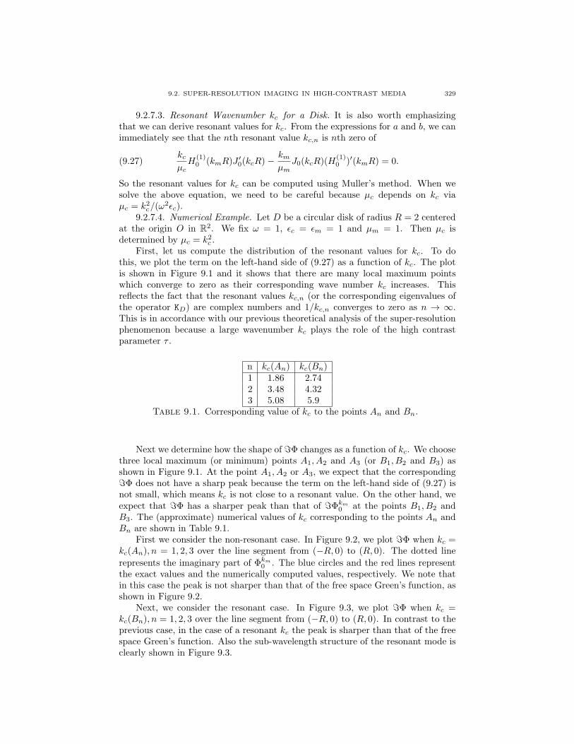
9.2. SUPER-RESOLUTION IMAGING IN HIGH-CONTRAST MEDIA 329
9.2.7.3. Resonant Wavenumber kc for a Disk. It is also worth emphasizingthat we can derive resonant values for kc. From the expressions for a and b, we canimmediately see that the nth resonant value kc,n is nth zero of
(9.27)kcµcH
(1)0 (kmR)J
′0(kcR)−
kmµm
J0(kcR)(H(1)0 )′(kmR) = 0.
So the resonant values for kc can be computed using Muller’s method. When wesolve the above equation, we need to be careful because µc depends on kc viaµc = k2c/(ω
2ǫc).9.2.7.4. Numerical Example. Let D be a circular disk of radius R = 2 centered
at the origin O in R2. We fix ω = 1, ǫc = ǫm = 1 and µm = 1. Then µc isdetermined by µc = k2c .
First, let us compute the distribution of the resonant values for kc. To dothis, we plot the term on the left-hand side of (9.27) as a function of kc. The plotis shown in Figure 9.1 and it shows that there are many local maximum pointswhich converge to zero as their corresponding wave number kc increases. Thisreflects the fact that the resonant values kc,n (or the corresponding eigenvalues ofthe operator KD) are complex numbers and 1/kc,n converges to zero as n → ∞.This is in accordance with our previous theoretical analysis of the super-resolutionphenomenon because a large wavenumber kc plays the role of the high contrastparameter τ .
n kc(An) kc(Bn)1 1.86 2.742 3.48 4.323 5.08 5.9
Table 9.1. Corresponding value of kc to the points An and Bn.
Next we determine how the shape of ℑΦ changes as a function of kc. We choosethree local maximum (or minimum) points A1, A2 and A3 (or B1, B2 and B3) asshown in Figure 9.1. At the point A1, A2 or A3, we expect that the correspondingℑΦ does not have a sharp peak because the term on the left-hand side of (9.27) isnot small, which means kc is not close to a resonant value. On the other hand, weexpect that ℑΦ has a sharper peak than that of ℑΦkm0 at the points B1, B2 andB3. The (approximate) numerical values of kc corresponding to the points An andBn are shown in Table 9.1.
First we consider the non-resonant case. In Figure 9.2, we plot ℑΦ when kc =kc(An), n = 1, 2, 3 over the line segment from (−R, 0) to (R, 0). The dotted line
represents the imaginary part of Φkm0 . The blue circles and the red lines representthe exact values and the numerically computed values, respectively. We note thatin this case the peak is not sharper than that of the free space Green’s function, asshown in Figure 9.2.
Next, we consider the resonant case. In Figure 9.3, we plot ℑΦ when kc =kc(Bn), n = 1, 2, 3 over the line segment from (−R, 0) to (R, 0). In contrast to theprevious case, in the case of a resonant kc the peak is sharper than that of the freespace Green’s function. Also the sub-wavelength structure of the resonant mode isclearly shown in Figure 9.3.

330 9. SUPER-RESOLUTION IMAGING
kc
0 2 4 6 8 100
0.1
0.2
0.3
0.4
0.5
0.6
0.7
0.8
A3
A2
A1
B3
B2
B1
Figure 9.1. The plot for the term on the left-hand side of (9.27)as a function of kc. D is a disk with radius R = 2. The parametersare ω = 1, εm = 1, εc = 1, µm = 1 and µc is determined by µc =k2c/(εcω
2). Three local maximums (or minimums) are marked asAn (or Bn), respectively.
Code Super-resolution in High Contrast Media was used to generate the nu-merical results shown in Table 9.1 and Figures 9.1, 9.2, and 9.3.
9.3. Super-Resolution in Resonant Structures
By modifying the homogeneous spaces with sub-wavelength resonators, we canintroduce propagating sub-wavelength resonance modes to the space which encodesub-wavelength information in a neighborhood of the space embedded by the sub-wavelength resonators, thus yielding a Green’s function whose imaginary part ex-hibits sub-wavelength peaks, thereby breaking the resolution limit (or diffractionlimit) in the homogeneous space. In this section, using the fact that plasmonicparticles are ideal sub-wavelength resonators, we consider the possibility of super-resolution by using a system of identical plasmonic particles.
9.3.1. Multiple Plasmonic Nanoparticles. We consider the scattering ofan incident time harmonic wave ui by multiple weakly coupled plasmonic nanopar-ticles in three dimensions. For ease of exposition, we consider the case of L particleswith an identical shape and use the Helmholtz equation for light propagation.
We write Dl = zl + δD, l = 1, 2, . . . , L, where D is centered at the origin.
Moreover, we denote D0 = δD as our reference nanoparticle and let
D =
L⋃
l=1
Dl, εD = εmχ(R3\D) + εcχ(D), µD = µmχ(R
3\D) + µcχ(D).
We assume that the following conditions hold.

9.3. SUPER-RESOLUTION IN RESONANT STRUCTURES 331
-2 -1.5 -1 -0.5 0 0.5 1 1.5 2-1
-0.5
0
0.5
1
1.5
-=)theo
-=)num
-=)0
-2 -1.5 -1 -0.5 0 0.5 1 1.5 2-1
-0.5
0
0.5
1
1.5
-=)theo
-=)num
-=)0
-2 -1.5 -1 -0.5 0 0.5 1 1.5 2-1
-0.5
0
0.5
1
1.5
-=)theo
-=)num
-=)0
Figure 9.2. The plot for ℑΦ when kc = kc(An), n = 1, 2, 3 overthe line segment from (−R, 0) to (R, 0). The dotted line represents
the imaginary part of Φkm0 . The blue circles and the red linesrepresent the exact values and the numerically computed values,respectively. In this case the peak is not sharper than that of thefree space Green’s function.
Condition 9.13. We assume that the numbers εm, µm, εc, µc are dimensionless
and are of order one. We also assume that the particle D has size of order one andω is dimensionless and is of order o(1).

332 9. SUPER-RESOLUTION IMAGING
-2 -1.5 -1 -0.5 0 0.5 1 1.5 2-1
-0.5
0
0.5
1
1.5
-=)theo
-=)num
-=)0
-2 -1.5 -1 -0.5 0 0.5 1 1.5 2-1
-0.5
0
0.5
1
1.5
-=)theo
-=)num
-=)0
-2 -1.5 -1 -0.5 0 0.5 1 1.5 2-1
-0.5
0
0.5
1
1.5
-=)theo
-=)num
-=)0
Figure 9.3. The plot for ℑΦ when kc = kc(Bn), n = 1, 2, 3 overthe line segment from (−R, 0) to (R, 0). The dotted line represents
the imaginary part of Φkm0 . The blue circles and the red linesrepresent the exact values and the numerically computed values,respectively. In this case the peak is sharper than that of the freespace Green’s function. Also the sub-wavelength structure of theresonant mode is clearly shown.
Condition 9.14. Let
(9.28) λ =µm + µc
2(µm − µc).
9.3. SUPER-RESOLUTION IN RESONANT STRUCTURES 333
We assume that λ 6= 0 or equivalently, µc 6= −µm.
Condition 9.15. The size δ of the particles is a small parameter and thedistances between neighboring particles are of order one.
The scattering problem can be modeled by the following Helmholtz equation:
(9.29)
∇ · 1
µD∇u+ ω2εDu = 0 in R3\∂D,
u+ − u− = 0 on ∂D,
1
µm
∂u
∂ν
∣∣∣∣+
− 1
µc
∂u
∂ν
∣∣∣∣−= 0 on ∂D,
us := u− ui satisfies the Sommerfeld radiation condition.
Let
ui(x) = e√−1kmd·x,
Fl,1(x) = −ui(x)∣∣∂Dl
= −e√−1kmd·x∣∣
∂Dl,
Fl,2(x) = −∂ui
∂ν(x)
∣∣∣∣∂Dl
= −√−1kme
√−1kmd·xd · ν(x)∣∣∂Dl
,
and define the operator KkDp,Dlby
KkDp,Dl[ψ](x) =
∫
∂Dp
∂Γk(x− y)
∂ν(x)ψ(y)dσ(y), x ∈ ∂Dl.
Analogously, we define
SkDp,Dl[ψ](x) =
∫
∂Dp
Γk(x− y)ψ(y)dσ(y), x ∈ ∂Dl.
The solution u of (9.29) can be represented as follows:
u(x) =
ui(x) +
L∑
l=1
SkmDl[ψl](x), x ∈ R3\D,
L∑
l=1
SkcDl[φl](x), x ∈ D,
where φl, ψl ∈ H− 12 (∂Dl) satisfy the following system of integral equations
SkmDl[ψl]− SkcDl
[φl] +∑
p 6=lSkmDp,Dl
[ψp] = Fl,1,
1
µm
(12I + (KkmDl
)∗)[ψl] +
1
µc
(12I − (KkcDl
)∗)[φl]
+1
µm
∑
p 6=lKkmDp,Dl
[ψp] = Fl,2,
and
Fl,1 = −ui on ∂Dl,
Fl,2 = − 1
µm
∂ui
∂νon ∂Dl.

334 9. SUPER-RESOLUTION IMAGING
9.3.2. First-Order Correction to Plasmonic Resonances and Field Be-havior at Plasmonic Resonances in the Multi-Particle Case. We considerthe scattering in the quasi-static regime, i.e., when the incident wavelength is muchgreater than one. With proper dimensionless analysis, we can assume that ω ≪ 1.As a consequence, SkcD is invertible. Note that
φl = (SkcDl)−1(SkmDl
[ψl] +∑
p 6=lSkmDp,Dl
[ψp]− Fl,1).
We obtain the following equation for ψl’s,
AD(w)[ψ] = f,
where
AD(w) =
AD1(ω)AD2
(ω). . .
ADL(ω)
+
0 A1,2(ω) . . . A1,L(ω)A2,1(ω) 0 . . . A2,L(ω)
... . . . 0...
AL,1(ω) . . . AL,L−1(ω) 0
,
ψ =
ψ1
ψ2
...ψL
, f =
f1f2...fL
,
with
(9.30) ADl(ω) =
1
µm
(12I + (KkmDl
)∗)+
1
µc
(12I − (KkcDl
)∗)(SkcDl
)−1SkmDl,
and
Al,p(ω) =1
µc
(12I − (KkcDl
)∗)(SkcDl
)−1SkmDp,Dl+
1
µmKkmDp,Dl
,
fl = Fl,2 +1
µc
(12I − (KkcDl
)∗)(SkcDl
)−1[Fl,1].
For j = 1, . . . , L, letH∗(∂Dj) andH(∂Dj) be respectively defined by (2.18) and(2.20) with Ω replaced with Dj . We first consider the operators SkDj
and (KkDj)∗.
The following asymptotic expansions hold. Its proof is immediate.
Lemma 9.16. (i) Regarded as operators from H∗(∂Dj) into H(∂Dj), wehave
SkDj= S0
Dj+ kSDj ,1 + k2SDj ,2 +O(k3δ3),
where S0Dj
= O(1) and SDj ,m = O(δm);
(ii) Regarded as operators from H(∂Dj) into H∗(∂Dj), we have
(SkDj)−1 = (S0
Dj)−1 + kBDj ,1 + k2BDj ,2 +O(k3δ3),
where S−1Dj
= O(1) and BDj ,m = O(δm);
(iii) Regarded as operators from H∗(∂Dj) into H∗(∂Dj), we have
(KkDj)∗ = (K0
Dj)∗ + k2O(δ2),
where (K0Dj
)∗ = O(1).
We also need the following result.

9.3. SUPER-RESOLUTION IN RESONANT STRUCTURES 335
Lemma 9.17. (i) Regarded as an operator from H∗(∂Dj) into H(∂Dl) wehave,
SkDj ,Dl= Sj,l,0,0 + Sj,l,0,1 + Sj,l,0,2 + kSj,l,1 + k2Sj,l,2,0 +O(δ4) +O(k2δ2).
Moreover,
Sj,l,m,n = O(δn+1).
(ii) Regarded as an operator from H∗(∂Dj) into H∗(∂Dl), we have
KkDj ,Dl= Kj,l,0,0 +O(k2δ2).
Moreover,
Kj,l,0,0 = O(δ2).
Finally, the following asymptotic expansions hold.
Lemma 9.18. (i) Regarded as operators from H∗(∂Dj) into H∗(∂Dj), wehave
ADj(ω) = ADj ,0 +O(δ2ω2),
(ii) Regarded as operators from H∗(∂Dl) into H∗(∂Dp), we have
Al,p(ω) =1
µc
(12I−(K0
Dl)∗)(S0Dl)−1(Sp,l,0,1+Sp,l,0,2
)+
1
µmKp,l,0,0+O(δ2ω2)+O(δ4).
Moreover,
(12I − (K0
Dl)∗) (S0
Dl)−1 Sp,l,0,1 = O(δ2),
(12I − (K0
Dl)∗) (S0
Dl)−1 Sp,l,0,2 = O(δ3),
Kp,l,0,0 = O(δ2).
Proof. The proof of (i) follows from Lemma 9.16. We now prove (ii). Recallthat
1
2I − (KkcDl
)∗ =1
2I − (K0
Dl)∗ +O(δ2ω2),
(SkcDl)−1 = (S0
Dl)−1 − kc(S0
Dl)−1SDl,1(S0
Dl)−1 +O(δ2ω2),
SkmDp,Dl= Sp,l,0,0 + Sp,l,0,1 + Sp,l,0,2 + kmSp,l,1 + k2mSp,l,2,0 +O(δ4) +O(ω2δ2)
KkmDp,Dl= Kp,l,0,0 +O(ω2δ2).
Using the identity
(12I − (K0
Dl)∗)(S0Dl)−1[χ(Dl)] = 0,

336 9. SUPER-RESOLUTION IMAGING
we can derive that
Al,p(ω) =1
µc
(12I − (K0
Dl)∗)(SkcDl
)−1SkmDp,Dl+
1
µmKp,l,0,0 +O(δ2ω2)
=1
µc
(12I − (K0
Dl)∗)(S0Dl)−1SkmDp,Dl
+1
µmKp,l,0,0 +O(δ2ω2)
=1
µc
(12I − (K0
Dl)∗)(S0Dl)−1(Sp,l,0,0 + Sp,l,0,1 + Sp,l,0,2 + kmSp,l,1 + k2mSp,l,2,0 +O(δ4)
)
+1
µmKp,l,0,0 +O(δ2ω2)
=1
µc
(12I − (K0
Dl)∗)(S0Dl)−1(Sp,l,0,1 + Sp,l,0,2
)+
1
µmKp,l,0,0 +O(δ2ω2) +O(δ4).
The rest of the lemma follows from Lemmas 9.16 and 9.17.
Denote by H∗(∂D) = H∗(∂D1) × . . . × H∗(∂DL), which is equipped with theinner product
〈ψ, φ〉H∗ =L∑
l=1
〈ψl, φl〉H∗(∂Dl).
With the help of Lemma 9.18, the following result is obvious.
Lemma 9.19. Regarded as an operator from H∗(∂D) into H∗(∂D), we have
A(ω) = AD,0 +AD,1 +O(ω2δ2) +O(δ4),
where
AD,0 =
AD1,0
AD2,0
. . .ADL,0
, AD,1 =
0 AD,1,12 AD,1,13 . . .AD,1,21 0 AD,1,23 . . .
. . .AD,1,L1 . . . AD,1,LL−1 0
with
ADl,0 =( 1
2µm+
1
2µc
)I − (
1
µc− 1
µm)(K0
Dl)∗,
AD,1,pq =1
µc
(12I − (K0
Dp)∗)(S0Dp
)−1(Sq,p,0,1 + Sq,p,0,2
)+
1
µmKq,p,0,0.
It is evident that
(9.31) AD,0[ψ] =∞∑
j=0
L∑
l=1
τj〈ψ, ϕj,l〉H∗ϕj,l,
where
τj =1
2µm+
1
2µc−( 1
µc− 1
µm
)λj ,(9.32)
ϕj,l = ϕjel(9.33)
with el being the standard basis of RL and (λj , ϕj) being the eigenvalues andassociated eigenfunctions of the operator (K0
D1)∗.
We consider A(ω) as a perturbation to the operator AD,0 for small ω andsmall δ. Using a standard perturbation argument, we can derive the perturbedeigenvalues and eigenfunctions.

9.3. SUPER-RESOLUTION IN RESONANT STRUCTURES 337
In what follows, we only use the first order perturbation theory and derive theleading order term, i.e., the perturbation due to the term AD,1. For each l, wedefine an L× L matrix Rl by letting
Rl,pq =⟨AD,1[ϕl,p], ϕl,q
⟩H∗ ,
=⟨AD,1[ϕlep], ϕleq
⟩H∗,
=⟨AD,1,pq[ϕl], ϕl
⟩H∗ .
Lemma 9.20. The matrix Rl = (Rl,pq)p,q=1,...,L has the following explicit ex-pression:
Rl,pp = 0,
Rl,pq =3
4πµc(λj −
1
2)
∑
|α|=|β|=1
∫
∂D0
∫
∂D0
(zp − zq)α+β
|zp − zq|5xαyβϕl(x)ϕl(y)dσ(x)dσ(y)
+( 1
4πµc− 1
4πµm
)(λj −
1
2)
∫
∂D0
∫
∂D0
x · y|zp − zq|3
ϕl(x)ϕl(y)dσ(x)dσ(y)
= O(δ3), p 6= q.
Proof. It is clear that Rl,pp = 0. For p 6= q, we have
Rl,pq = RIl,pq +RIIl,pq +RIIIl,pq,
where
RIl,pq =1
µc
⟨(12I − (K0
Dp)∗)(S0Dp
)−1Sq,p,0,1[ϕl], ϕl⟩H∗(∂Dl)
,
RIIl,pq =1
µc
⟨(12I − (K0
Dp)∗)(S0Dp
)−1Sq,p,0,2[ϕl], ϕl⟩H∗(∂Dl)
,
RIIIl,pq =1
µm
⟨Kq,p,0,0[ϕl], ϕl
⟩H∗(∂Dl)
.
We first consider RIl,pq. By the following identity
(12I − (K0
Dp)∗)SDl
[ϕl] = S0Dl
(12I −K0
Dp
)[ϕl] = (λj −
1
2)ϕl,
we obtain
RIl,pq = − 1
µc
⟨(12I − (K0
Dp)∗)(S0Dp
)−1Sq,p,0,1[ϕl],S0Dl[ϕl]⟩L2(∂Dl)
,
=1
µc(λj −
1
2)⟨Sq,p,0,1[ϕl],S0
Dl[ϕl]⟩L2(∂Dl)
.
Using the explicit representation of Sq,p,0,1, we further conclude that
RIl,pq = 0.

338 9. SUPER-RESOLUTION IMAGING
Similarly, we have
RIIl,pq =1
µc(λj −
1
2)⟨Sq,p,0,2[ϕl],S0
Dl[ϕl]⟩L2(∂Dl)
,
=1
µc(λj −
1
2)
∑
|α|=|β|=1
∫
∂D0
∫
∂D0
(3(zp − zq)α+β
4π|zp − zq|5xαyβ +
δαβxαyβ
4π|zp − zq|3)ϕl(x)ϕl(y)dσ(x)dσ(y)
=3
4πµc(λj −
1
2)
∑
|α|=|β|=1
∫
∂D0
∫
∂D0
(zp − zq)α+β
|zp − zq|5xαyβϕl(x)ϕl(y)dσ(x)dσ(y)
+1
4πµc(λj −
1
2)∑
|α|=1
∫
∂D0
∫
∂D0
1
|zp − zq|3xαyαϕl(x)ϕl(y)dσ(x)dσ(y).
Finally, note that
Kq,p,0,0[ϕl] =1
4π|zp − zq|3a · ν(x) = 1
4π|zp − zq|33∑
m=1
amνm(x),
where am =⟨(y − zq)m, ϕl
⟩L2(∂Dq)
, and a = (a1, a2, a3)t.
Therefore, we have
RIIIl,pq = − 1
µm
⟨Kq,p,0,0[ϕl], ϕl
⟩H∗(∂Dl)
= − 1
4π|zp − zq|3µm⟨a · ν(x), ϕl
⟩H∗(∂Dl)
= − 1
4π|zp − zq|3µm
⟨(12I − (K0
Dp)∗)(S0Dp
)−1(a · (x− zp)), ϕl
⟩
H∗(∂Dl)
= − 1
4π|zp − zq|3µm(λj −
1
2)⟨a · (x− zp), ϕl
⟩L2(∂Dp)
= − 1
4π|zp − zq|3µm(λj −
1
2)
∫
∂D0
∫
∂D0
x · yϕl(x)ϕl(y)dσ(x)dσ(y).
This completes the proof of the lemma.
We now have an explicit formula for the matrix Rl. It is clear that Rl issymmetric, but not self-adjoint. For ease of presentation, we assume the followingcondition.
Condition 9.21. Rl has L-distinct eigenvalues.
We remark that Condition 9.21 is not essential for our analysis. Without thiscondition, the perturbation argument is still applicable, but the results may bequite complicated. We refer to [293] for a complete description of the perturbationtheory.
Let τj,l and Xj,l = (Xj,l,1, . . . , Xj,l,L)t, l = 1, 2, . . . , L, be the eigenvalues and
normalized eigenvectors of the matrix Rj . We remark that each Xj,l may be com-plex valued and may not be orthogonal to other eigenvectors.
Under perturbation, each τj splits into the following L eigenvalues of A(ω),
(9.34) τj,l(ω) = τj + τj,l +O(δ4) +O(ω2δ2).

9.3. SUPER-RESOLUTION IN RESONANT STRUCTURES 339
The associated perturbed eigenfunctions have the following form
(9.35) ϕj,l(ω) =
L∑
p=1
Xj,l,pepϕj +O(δ4) +O(ω2δ2).
We are interested in solving the equation AD(ω)[ψ] = f when ω is close to theresonance frequencies, i.e., when τj(ω) are very small for some j’s. In this case, themajor part of the solution would be based on the excited resonance modes ϕj,l(ω).
For this purpose, we introduce the index set of resonances J just as we did in(7.12) for the single particle case.
Definition 9.22. We call J ⊂ N index set of resonances if the τj,l(ω)’s areclose to zero when j ∈ J and are bounded from below when j ∈ Jc. More precisely,we choose a threshold number η0 > 0 independent of ω such that
|τj,l(ω)| ≥ η0 > 0 for j ∈ Jc.
For simplicity, we assume that the following conditions hold.
Condition 9.23. Each eigenvalue λj, j ∈ J , of the operator (K0D1
)∗ is simple.
Moreover, we have ω2 ≪ δ.
We define
PJ(ω)ϕj,m(ω) =
ϕj,m(ω), j ∈ J,0, j ∈ Jc.
In fact,
(9.36) PJ(ω) =∑
j∈JPj(ω) =
∑
j∈J
1
2π√−1
∫
γj
(ξ −AD(ω))−1dξ,
where γj is a Jordan curve in the complex plane enclosing only the eigenvaluesτj,l(ω) for l = 1, 2, . . . , L among all the eigenvalues.
To obtain an explicit representation of PJ(ω), we consider the adjoint operatorAD(ω)
∗. By a similar perturbation argument, we can obtain its perturbed eigen-value and eigenfunctions. Note that the adjoint matrix Rtj = Rj has eigenvalues τj,land corresponding eigenfunctions Xj,l. Then the eigenvalues and eigenfunctions ofAD(ω)
∗ have the following form
τj,l(ω) = τj + τj,l +O(δ4) +O(ω2δ2),
ϕj,l(ω) = ϕj,l +O(δ4) +O(ω2δ2),
where
ϕj,l =
L∑
p=1
Xj,l,pepϕj
with Xj,l,p being a multiple of Xj,l,p.We normalize ϕj,l in a way such that the following holds:
〈ϕj,p, ϕj,q〉H∗(∂D) = δpq,
which is also equivalent to the following condition
Xj,ptXj,q = δpq.
Then, we can show that the following result holds.
340 9. SUPER-RESOLUTION IMAGING
Lemma 9.24. In the space H∗(∂D), as ω goes to zero, we have
f = ωf0 +O(ω2δ32 ),
where f0 = (f0,1, . . . , f0,L)t with
f0,l = −√−1
√εmµme
√−1kmd·zl(
1
µmd · ν(x) + 1
µc
(12I − (K0
Dl)∗)(S0Dl)−1[d · (x− z)]
)= O(δ
32 ).
Proof. We first show that
‖u‖H∗(∂D0) = δ32+m‖u‖H∗(∂D), ‖u‖H(∂D0) = δ
12+m‖u‖H(∂D)
for any homogeneous function u such that u(δx) = δmu(x). Indeed, we have
η(u)(x) = δmu(x). Since ‖η(u)‖H∗(∂D) = δ−32 ‖u‖H∗(∂D0), we obtain
‖u‖H∗(∂D0) = δ32 ‖η(u)‖H∗(∂D) = δ
32+m‖u‖H∗(∂D),
which proves our first claim. The second claim follows in a similar way. Using thisresult, we arrive at the desired asymptotic result.
Denote by Z = (Z1, . . . , ZL), where Zj =√−1kme
√−1kmd·zj . We are ready topresent our main result in this section.
Theorem 9.25. Under Conditions 9.13, 9.14, 9.15, and 9.21, the scatteredfield due to L plasmonic particles in the quasi-static regime has the following rep-resentation
us =
L∑
l
SkmDl[ψl],
where ψ = (ψ1, . . . , ψL)t has the following asymptotic expansion:
ψ =∑
j∈J
L∑
l=1
⟨f, ϕj,l(ω)
⟩H∗ϕj,l(ω)
τj,l(ω)+AD(ω)
−1(PJc(ω)f)
=∑
j∈J
L∑
l=1
〈d · ν(x), ϕj〉H∗(∂D0)ZXj,l ϕj,l +O(ω2δ32 )
λ− λj +(
1µc
− 1µm
)−1τj,l +O(δ4) +O(δ2ω2)
+O(ωδ32 ).
Proof. The proof is similar to that of Theorem 7.15.
As a consequence, the following result holds.
Corollary 9.26. With the same notation as in Theorem 9.25 and under theadditional condition that
minj∈J
|τj,l(ω)| ≫ ωqδp,
for some integer p and q, and
τj,l(ω) = τj,l,p,q + o(ωqδp),
we have
ψ =∑
j∈J
L∑
l=1
〈d · ν(x), ϕj〉H∗(∂D0)ZXj,l ϕj,l +O(ω2δ32 )
τj,l,p,q+O(ωδ
32 ).
9.3.3. Super-Resolution by Using Plasmonic Nanoparticles.

9.3. SUPER-RESOLUTION IN RESONANT STRUCTURES 341
9.3.3.1. Asymptotic Expansion of the Scattered Field. In order to illustrate thesuperfocusing phenomenon, we set
ui(x) = Γkm(x− x0) = −e√−1km|x−x0|
4π|x− x0|.
Lemma 9.27. In the space H∗(∂D), as ω goes to zero, we have
f = f0 +O(ωδ32 ) +O(δ
52 ),
where f0 = (f0,1, . . . , f0,L)t with
f0,l = − 1
4π|zl − x0|3(
1
µm(zl − x0) · ν(x) +
1
µc(1
2I − (K0
Dl)∗)(S0
Dl)−1[(zl − x0) · (x− zl)]
)= O(δ
32 ).
Proof. Recall that
fl = Fl,2 +1
µc
(12I − (KkcDl
)∗)(SkcDl
)−1[Fl,1].
We can show that
Fl,2 = − 1
µm
∂ui
∂ν= − 1
4πµm|zl − x0|3(zl−x0) ·ν(x)+O(δ
52 )+O(ωδ
32 ) in H∗(∂Dl).
Besides,
ui(x)|∂Dl= −e
√−1km|zl−x0|
4π|zl − x0|χ(∂Dl)+
1
4π|zl − x0|3(zl−x0)·(x−zl)+O(δ
52 )+O(ωδ
32 ) in H(∂Dl).
Using the identity ( 12I − (K0Dl)∗)(S0
Dl)−1[χ(∂Dl)] = 0, we obtain that
1
µc
(12I−(KkcDl
)∗)(SkcDl
)−1[Fl,1] = − 1
4π|zl − x0|3µc(1
2I−(K0
Dl)∗)(S0
Dl)−1[(zl−x0)·(x−zl)].
This completes the proof of the lemma.
We now derive an asymptotic expansion of the scattered field in an intermediateregime which is neither too close to the plasmonic particles nor too far away. Moreprecisely, we consider the following domain
Dδ,k =x ∈ R3; min
1≤l≤L|x− zl| ≫ δ, max
1≤l≤L|x− zl| ≪
1
k
.
Lemma 9.28. Let ψl ∈ H∗(∂Dl) and let v(x) = SkDl[ψl](x). Then we have for
x ∈ Dδ,k,
v(x) = Γk(x− zl)( 1
|x− zl|−√−1k
) x− zl|x− zl|
·∫
∂D0
yψl(y)dσ(y) +O(δ52 )‖ψl‖H∗(∂Dl)
+Γk(x− zl)
∫
∂D0
ψl(y)dσ(y).
Moreover, the following estimates hold
v(x) = O(δ32 ) if
∫
∂D0
ψl(y)dσ(y) = 0,
v(x) = O(δ12 ) if
∫
∂D0
ψl(y)dσ(y) 6= 0.

342 9. SUPER-RESOLUTION IMAGING
Proof. We only consider the case when l = 0. The other case follows similarlyor by coordinate translation. We have
v(x) = SkD[ψ](x) =∫
∂D0
Γk(x− y)ψ(y)dσ(y) = −∫
∂D0
e√−1k|x−y|
4π|x− y| ψ(y)dσ(y).
Since
Γk(x− y) = Γk(x) +∑
|α=1|
∂Γk(x)
∂yαyα +
∑
m≥2
∑
|α=m|
∂mΓk(x)
∂yαyα,
and
∂Γk(x)
∂yα= −e
√−1k|x|
4π|x|( 1
|x| −√−1k
) x|x| = Γk(x)
( 1
|x| −√−1k
)xα|x| ,
we obtain the required identity for the case l = 0. The estimate follows from thefact that
‖yα‖H(∂D0) = O(δ2|α|+1
2 ).
This completes the proof of the lemma.
Denote by
Sj,l(x, k) = Γk(x− zl)x− zl
|x− zl|2·∫
∂D0
yϕj(y)dσ(y),
Sl(x, k) = Γk(x− zl)
∫
∂D0
ϕ0(y)dσ(y),
Hj,l(x0) = − 1
4π|zl − x0|3⟨(zl − x0) · ν(x), ϕj
⟩H∗(∂D0)
.
It is clear that the following size estimates hold
Sj,l(x, k) = O(δ32 ), Sl(x, k) = O(δ
12 ), Hj,l(x0) = O(δ
32 ) for j 6= 0, H0,l(x0) = 0.
Theorem 9.29. Under Conditions 9.13, 9.14, 9.15, and 9.21, the Green func-tion Φkm(x, x0) in the presence of L plasmonic particles has the following represen-tation in the quasi-static regime: for x ∈ Dδ,km ,
Φkm(x, x0) = Γkm(x− x0)
+∑
j∈J
L∑
l=1
Hj,p(x0)Xj,l,pXj,l,qSj,q(x, km) +O(δ4) +O(ωδ3)
λ− λj +(
1µc
− 1µm
)−1τj,l +O(δ4) +O(δ2ω2)
+O(δ3).
Proof. With ui(x) = Γkm(x− x0), we have
ψ =∑
j∈J
∑
1≤l≤Laj,lϕj,l +
∑
1≤l≤La0,lϕ0,l +O(δ
32 ),
where
aj,l = 〈f, ϕj,l〉H∗(∂D) = 〈f0, ϕj,l〉H∗(∂D) +O(ωδ32 ) +O(δ
52 ),
= (1
µc− 1
µm)Xj,l,pHj,p(x0) +O(ωδ
32 ) +O(δ
52 ),
a0,l = 〈f, ϕ0,l〉H∗(∂D) = O(δ52 ).

9.3. SUPER-RESOLUTION IN RESONANT STRUCTURES 343
By Lemma 9.28,
SkmD [ϕj,l](x) =∑
1≤p≤LSkmD [Xj,l,pϕjep](x) =
∑
1≤p≤LXj,l,pSkmDp
[ϕj ](x)
=∑
1≤p≤LXj,l,pSj,p(x, km) +O(δ
52 ) +O(ωδ
32 ).
On the other hand, for j = 0, we have
SkmD [ϕ0,l](x) = O(δ12 ),
τ0,l(ω) = τ0 +O(δ4) +O(δ2ω2) = O(1).
Therefore, we can deduce that
us = SkmD [ψ](x) =∑
j∈J
∑
1≤l≤Laj,lSkmD [ϕj,l] +
∑
1≤l≤La0,lSkmD [ϕ0,l] +O(δ3),
=∑
j∈J
L∑
l=1
1
τj,l(ω)
((1
µc− 1
µm)Hj,p(x0)Xj,l,pXj,l,qSj,q(x, km) +O(ωδ3) +O(δ4)
)
+O(δ3),
=∑
j∈J
L∑
l=1
Hj,p(x0)Xj,l,pXj,l,qSj,q(x, km) +O(ωδ3) +O(δ4)
λ− λj +(
1µc
− 1µm
)−1τj,l +O(δ4) +O(δ2ω2)
+O(δ3).
9.3.4. Asymptotic Expansion of the Imaginary Part of the Green’sFunction. As a consequence of Theorem 9.29, we obtain the following result onthe imaginary part of the Green function.
Theorem 9.30. Assume the same conditions as in Theorem 9.29. Under theadditional assumption that
λ− λj +( 1
µc− 1
µm
)−1τj,l ≫ O(δ4) +O(δ2ω2),
ℜ(λ− λj +
( 1
µc− 1
µm
)−1τj,l
). ℑ
(λ− λj +
( 1
µc− 1
µm
)−1τj,l
)
for each l and j ∈ J , we have
ℑΦkm(x, x0) = ℑΓkm(x− x0) +O(δ3) +
∑
j∈J
L∑
l=1
ℜ(Hj,p(x0)Xj,l,pXj,l,qSj,q(x, 0) +O(ωδ3) +O(δ4)
)
×ℑ
1
λ− λj +(
1µc
− 1µm
)−1τj,l
,
where x, x0 ∈ Dδ,km .
Note that ℜ(Hj,p(x0)Xj,l,pXj,l,qSj,q(x, 0)
)= O(δ3). Under the conditions in
Theorem 9.30, if we have additionally that
ℑ
1
λ− λj +(
1µc
− 1µm
)−1τj,l
= O(
1
δ3)

344 9. SUPER-RESOLUTION IMAGING
for some plasmonic frequency ω, then the term in the expansion of ℑΦkm(x, x0)which is due to resonance has size one and exhibits a sub-wavelength peak withwidth of order one. This breaks the diffraction limit 1/km in the free space. We alsonote that the term ℑΓkm(x− x0) has size O(ω). Thus, we can conclude that super-resolution (super-focusing) can indeed be achieved by using a system of plasmonicparticles.
Remark 9.31. The results of this section on the super-resolution effect obtainedby using a finite system of plasmonic nanoparticles can be extended to the fullMaxwell equations.
9.4. Super-Resolution Based on Scattering Tensors
9.4.1. Multipolar Expansion. In this subsection we use the same notationas in Section (8.2). We consider for the sake of simplicity the two-dimensionalcase. We let BR := |x| < R and D be a small particle located at z ∈ BRwith electromagnetic parameters εc and µc. We set xi, i = 1, . . . , N to be equi-distributed points along the boundary ∂BR for N ≫ 1. The array of N elementsx1, . . . , xN is used to detect the particle. The array of elements x1, . . . , xN isoperating both in transmission and in reception. Let usj be the wave scattered byD = z + δB corresponding to the incident wave Γkm(x− xj).
From the multipolar expansion (2.258), it follows that
(9.37)usj(x) =
n+1∑
|l′|=0
n−|l′|+1∑
|l|=0
δ|l|+|l′|
l!l′!∂lΓkm(x− z)∂l
′
z Γkm(xj − z)Wll′
+O(δn+2) ,
where Wll′ is the scattering tensor defined by (2.257).Therefore, the entries aωij of the data matrix Aω introduced in (8.1) can be
approximated as follows:
(9.38) aωij = g(xi, z)Wg(xj , z)t +O(δn+2) ,
where g(xi, z) is a row vector of size (n+ 1)× (n+ 2)/2, which is given by
(9.39) g(xi, z) =( 1l!∂lΓkm(xi − z)
)|l|≤n ,
and W is defined by
(9.40) W =(δ|l|+|l′|Wll′
)|l|,|l′|≤n .
If δ is small, then high-order terms in (9.37) can be neglected. In this case, theanalysis of the data matrix reduces to the one in Section 8.2, which is based on thedipolar approximation (2.274). As δ increases, more and more multipolar termscould be included in formula (9.38) in order to approximate the data matrix. Forfixed δ, the number of multipolar terms (or the maximal resolving order) which canbe robustly reconstructed from the measured data depends only on the signal-to-noise ratio and can be estimated as a function of the signal-to-noise ratio [77].
In view of (9.39), the signal space of the data matrix Aω becomes richer. Theset of the singular vectors consists of the Green function and its derivatives. In orderto locate the particle, exactly the same imaging functionals constructed in Section8.2 can be used. They peak at the location of the particle. However, the significantsingular values are perturbed, even those associated with the dipolar approximation

9.5. CONCLUDING REMARKS 345
(2.274). Indeed, when δ is increasing, new significant singular values can merge.Those are related to higher-order multipolar terms. They can be expressed in terms
of the scattering tensors Wll′ . These new singular values, which are intermediatebetween the three larger ones (in the case of a single particle) and zero, containsome information on the particle and give a better approximation of its shape andelectromagnetic parameters.
9.4.2. Reconstruction Procedure. In this subsection we first present for-mulas for the reconstruction of the size and material parameters of the particlefrom the data matrix Aω. Then we introduce optimal control and dictionary-basedmatching approaches to identify the shape of the particle.
Once the location z of the particle is estimated for instance by using MUSICalgorithm, the matrix W can be recovered from the data matrix Aω. The size |D|and the electric permittivity ε can be estimated as follows:
|D| = 1
k2m|W(2,0),(0,0)|
and
εc =|W(2,0),(0,0)|ω2µm|D| .
By (2.266) we know that (Wll′)|l|=|l′|=1 is approximately the polarization tensorassociated with D and λ given by (2.264). Therefore, by (2.103) and (2.104) anequivalent ellipse can be computed and an estimate of µc can be found.
Once the equivalent ellipse is reconstructed we can use it as an initial guess andminimize using an optimal control scheme the discrepancy between the computedand measured matrix W; see [50]. The level set method can be implemented inorder to reconstruct separately closely spaced particles [40].
In [77], a dictionary matching approach is proposed. It is an alternative to theoptimal control approach. It relies on learning the geometric features containedin the matrix data. In the dictionary matching approach, we identify and classifya particle, knowing in advance that the latter belongs to a certain collection ofparticles. The method relies on computing the invariants under rigid motions fromthe extracted scattering tensors and allows us to handle the scaling within certainranges. A particle is classified by comparing its invariants with those of a set oflearned shapes at multiple-frequencies. The larger the frequency band used, thebetter the classification performance of the dictionary matching algorithm.
The reconstruction results obtained by the optimal control method and thedictionary matching approach are far beyond the resolution limit.
9.5. Concluding Remarks
In this chapter, we have provided a mathematical theory to explain the super-resolution mechanism in high-contrast media. We have investigated the behaviorof the Green’s functions of high-contrast media. Our resonance expansions of theGreen’s functions, which were first derived in [84], are the key to mathematicallyexplaining the super-resolution mechanism in high-contrast media. From (9.15)and (9.17), we have proved that the super-resolution is due to propagating sub-wavelength resonant modes. It is worth mentioning that in (9.15) and (9.17), wehave observed that a phenomenon of mixing of modes occurs. This is essentiallydue to the non-hermitian nature of the operator KD.


Part 4
Metamaterials


CHAPTER 10
Near-Cloaking
10.1. Introduction
To cloak a target is to make it invisible with respect to probing by electromag-netic or elastic waves. Extensive work has been produced on cloaking in the contextof electromagnetic and elastic waves. Many schemes for cloaking are currently un-der active investigation. These include interior cloaking, where the cloaking regionis inside the cloaking device, and exterior cloaking in which the cloaking region isoutside the cloaking device.
In this chapter, we focus on interior cloaking and describe effective near-cloaking structures for electromagnetic and elastic scattering problems. The focusof the next chapter will be placed on exterior cloaking.
In interior cloaking, the difficulty is to construct material parameter distribu-tions of a cloaking structure such that any target placed inside the structure isundetectable to waves. One approach is to use transformation optics (also calledthe scheme of changing variables) [306, 246, 146, 452, 257, 414]. The princi-ple behind transformation optics is to use a coordinate transformation to derivethe spatial dependent material parameters to guide the wave. Transformation op-tics takes advantage of the fact that the equations governing electromagnetic andacoustic wave propagation have transformation laws under change of variables; seeSubsection 2.14.4. They are form invariant under coordinate transformations. Thisallows one to design structures that bend waves around a hidden region, returningthem to their original path on the far side. The change of variables based cloakingmethod uses a singular transformation to boost the material properties so that itmakes a cloaking region look like a point to outside measurements. However, thistransformation induces the singularity of material constants in the transversal di-rection (also in the tangential direction in two dimensions), which causes difficultyboth in the theory and applications. To overcome this weakness, so called ‘near-cloaking’ is naturally considered, which is a regularization or an approximation ofsingular cloaking. Instead of the singular transformation, one can use a regularone to push forward the material parameters, in which a small ball is blown upto the cloaking region [302, 301]. Enhanced cloaking can be achieved by usinga cancellation technique [57, 58]. The first stage of this approach involves de-signing a multi-coated structure around a small perfect insulator to significantlyreduce its effect on boundary or scattering cross-section measurements. The multi-coating cancels the generalized polarization tensors or the scattering coefficients ofthe cloaking device. One then obtains a near-cloaking structure by pushing for-ward the multi-coated structure around a small object via the standard blow-uptransformation technique.
349

350 10. NEAR-CLOAKING
The purpose of this chapter is to review the cancellation technique. We firstdesign a structure coated around a particle to have vanishing generalized polariza-tion tensors of lower orders and show that the order of perturbation due to a smallparticle can be reduced significantly. We then obtain a near-cloaking structure bypushing forward the multi-coated structure around a small object via the usualblow-up transformation.
When considering near-cloaking for the Helmholtz equation, we construct struc-tures such that their first scattering coefficients vanish. Analogously to the quasi-static limit, we prove that, after applying transformation optics, structures withvanishing scattering coefficients enhance near-cloaking. We emphasize that such astructure achieves near-cloaking for a band of frequencies. We also show that near-cloaking for the Helmholtz equation becomes increasingly difficult as the cloakedobject becomes bigger or the operating frequency becomes higher. The difficultyscales inversely proportionally to the object diameter or the frequency.
Finally, the cancellation technique is extended to the full Maxwell equationsand the Lame system.
The results of this chapter are from [57, 58, 59, 1].
10.2. Near-Cloaking in the Quasi-Static Limit
To explain the principle of construction of cloaking structures, we review theresults on the quasi-static model obtained in [57].
Let Ω be a domain in R2 containing 0 possibly with multiple components withsmooth boundary. For a contrast λ, recall that the generalized polarization tensorsMαβ(λ,Ω) associated with Ω and λ are defined in (2.69).
Let Pm(x) be the complex-valued polynomial
(10.1) Pm(x) = (x1 +√−1x2)
m :=∑
|α|=mamα x
α +√−1
∑
|β|=mbmβ x
β .
Using polar coordinates x = re√−1θ, the above coefficients amα and bmβ can also be
characterized by
(10.2)∑
|α|=mamα x
α = rm cosmθ, and∑
|β|=mbmβ x
β = rm sinmθ .
We introduce the following combination of generalized polarization tensors us-ing the coefficients in (10.1):
M ccmn =
∑
|α|=m
∑
|β|=namα a
nβMαβ ,(10.3)
M csmn =
∑
|α|=m
∑
|β|=namα b
nβMαβ ,(10.4)
Mscmn =
∑
|α|=m
∑
|β|=nbmα a
nβMαβ ,(10.5)
Mssmn =
∑
|α|=m
∑
|β|=nbmα b
nβMαβ .(10.6)

10.2. NEAR-CLOAKING IN THE QUASI-STATIC LIMIT 351
For a given harmonic function H in R2, consider
(10.7)
∇·(σ0χ(R
2 \ Ω) + σχ(Ω))∇u = 0 in R2 ,
u(x)−H(x) = O(|x|−1) as |x| → ∞ ,
where σ0 and σ are conductivities (positive constants) of R2\Ω and Ω, respectively.If the harmonic function H admits the expansion
H(x) = H(0) +∞∑
n=1
rn(acn(H) cosnθ + asn(H) sinnθ
)
with x = (r cos θ, r sin θ), then, we have the following formula
(u−H)(x) = −∞∑
m=1
cosmθ
2πmrm
∞∑
n=1
(M ccmna
cn(H) +M cs
mnasn(H)
)
−∞∑
m=1
sinmθ
2πmrm
∞∑
n=1
(Mscmna
cn(H) +Mss
mnasn(H)
)as r = |x| → ∞ ,(10.8)
where M ccmn,M
csmn,M
scmn, and M
scmn are defined by (10.3)–(10.6).
In order to make u look like H for large |x|, we construct structures with van-ishing generalized polarization tensors for all |n|, |m| ≤ N . We call such structuresGPT-vanishing structures of orderN . To do so, we use a disc with multiple coatings.Let Ω be a disc of radius r1. For a positive integer N , let 0 < rN+1 < rN < · · · < r1and define
(10.9) Aj := rj+1 < r = |x| ≤ rj, j = 1, 2, . . . , N .
Let A0 = R2 \ Ω and AN+1 = r ≤ rN+1. Set σj to be the conductivity of Aj forj = 1, 2, . . . , N + 1, and σ0 = 1. Let
(10.10) σ =
N+1∑
j=0
σjχ(Aj) .
Because of the symmetry of the disc, one can easily see that
(10.11) M csmn[σ] =Msc
mn[σ] = 0 for all m,n ,
(10.12) M ccmn[σ] =Mss
mn[σ] = 0 if m 6= n ,
and
(10.13) M ccnn[σ] =Mss
nn[σ] for all n .
Let Mn =M ccnn, n = 1, 2, . . . , for the simplicity of notation. Let
(10.14) ζj :=σj − σj−1
σj + σj−1, j = 1, . . . , N + 1 .
One can prove that [57]
(10.15) |Mn| ≤ 2πnr2n1 for all n ∈ N.
The following is a characterization of GPT-vanishing structures. Again, see [57].
352 10. NEAR-CLOAKING
Proposition 10.1. If there are nonzero constants ζ1, . . . , ζN+1 (|ζj | < 1) andr1 > · · · > rN+1 > 0 such that
(10.16)
N+1∏
j=1
[1 ζjr
−2lj
ζjr2lj 1
]is an upper triangular matrix for l = 1, 2, . . . , N,
then (Ω, σ), given by (10.9), (10.10), and (10.14), is a GPT-vanishing structure oforder N , i.e., Ml = 0 for l ≤ N . More generally, if there are nonzero constantsζ1, ζ2, ζ3, . . . (|ζj | < 1) and r1 > r2 > r3 > . . . such that rn converges to a positivenumber, say r∞ > 0, and
(10.17)
∞∏
j=1
[1 ζjr
−2lj
ζjr2lj 1
]is an upper triangular matrix for every l,
then (Ω, σ), given by (10.9), (10.10), and (10.14), is a GPT-vanishing structurewith Ml = 0 for all l.
Let (Ω, σ) be a GPT-vanishing structure of order N of the form (10.10). Wetake r1 = 2 so that Ω is the disk of radius 2, and rN+1 = 1. We assume thatσN+1 = 0 which amounts to the structure being insulated along ∂B1. For smallδ > 0, let
(10.18) Ψ 1δ(x) =
1
δx, x ∈ R2 .
Then, (B2δ, σ Ψ 1δ) is a GPT-vanishing structure of order N and it is insulated on
∂Bδ.For a given domain Ω and a subdomain B ⋐ Ω, we introduce the Dirichlet-to-
Neumann map ΛΩ,B [σ] as
(10.19) ΛΩ,B [σ](f) = σ∂u
∂ν
∣∣∣∣∂Ω
,
where u is the solution to
(10.20)
∇ · σ∇u = 0 in Ω \B ,∂u
∂ν= 0 on ∂B ,
u = f on ∂Ω ,
where ν is the outward normal to ∂B. Note that with Ω = B2, ΛΩ,Bδ[σ Ψ 1
δ] may
be regarded as small perturbation of ΛΩ,∅[1] if Ml = 0 for all l ≤ N . A completeasymptotic expansion of ΛΩ,Bδ
[σ Ψ 1δ] as δ → 0 can be obtained and it can be
proved that
(10.21)∥∥∥ΛB2,Bδ
[σ Ψ 1
δ
]− ΛB2,∅[1]
∥∥∥ ≤ Cδ2N+2
for some constant C independent of δ, where the norm is the operator norm fromH1/2(∂Ω) into H−1/2(∂Ω). In fact, if f admits the Fourier expansion f(θ) =∑
n∈Z
fne√−1nθ, then we have
(ΛB2,Bδ
[σ Ψ 1
δ
]− ΛB2,∅[1]
)(f) =
∑
n∈Z
|n|(δ/2)2|n|M|n|2π|n| − (δ/2)2|n|M|n|
fne√−1nθ.

10.3. NEAR-CLOAKING FOR THE HELMHOLTZ EQUATION 353
From (10.15) , it follows that as δ → 0,
|Mn|δ2n ≤ Cδ2N+2 for all n ∈ N
for some constant C independent of n and hence, (10.21) holds; see [57]. We thenpush forward σ Ψ 1
δby the change of variables Fδ,
(10.22) Fδ(x) :=
( 3− 4δ
2(1− δ)+
1
4(1− δ)|x|) x|x| for 2δ ≤ |x| ≤ 2 ,
(12+
1
2δ|x|) x|x| for δ ≤ |x| ≤ 2δ ,
x
δfor |x| ≤ δ ,
in other words,
(10.23) (Fδ)⋆(σ Ψ 1δ) =
(DFδ)(σ Ψ 1δ)(DFδ)
t
| det(DFδ)| F−1
δ .
Note that Fδ maps |x| = δ onto |x| = 1, and is the identity on |x| = 2. So byinvariance of the Dirichlet-to-Neumann map, we have
(10.24) ΛB2,B1
[(Fδ)⋆(σ Ψ 1
δ)]= ΛB2,Bδ
[σ Ψ 1
δ
].
Identity (10.24) can be proved using the divergence theorem [146]. Thus we obtainthe following theorem from [57], which shows that, using GPT-vanishing structureswe achieve enhanced near-cloaking.
Theorem 10.2. Let the conductivity profile σ be a GPT-vanishing structure oforder N such that σN+1 = 0. There exists a constant C independent of δ such that
(10.25)∥∥∥ΛB2,B1
[(Fδ)⋆(σ Ψ 1
δ)]− ΛB2,∅[1]
∥∥∥ ≤ Cδ2N+2 .
Remark 10.3. It is worth emphasizing that the conductivities of the constructednear-cloaking devices are anisotropic. Nevertheless, they can be approximated byconcentric isotropic homogeneous coatings [39, 414]. The approximation is inthe sense that it minimizes the discrepancy between the associated Dirichlet-to-Neumann maps for only the first few eigenvectors.
Remark 10.4. If we consider the spectra of the Laplacian with Dirichlet orNeumann boundary conditions inside on one hand the near-cloaking device of orderN and on the other hand the homogeneous disk of conductivity one, then one canshow that the first eigenvalues are approximately the same (up to an error of orderof δ2N+2).
10.3. Near-Cloaking for the Helmholtz Equation
Analogously to the quasi-static case, in order to achieve enhanced near-cloakingfor the Helmholtz equation, we construct multi-coated structures such that theirfirst scattering coefficients vanish. Then by pushing forward the multi-coated struc-tures via the transformation optics, we obtain enhanced cloaking with respect toscattering cross-section measurements.
354 10. NEAR-CLOAKING
10.3.1. Scattering Coefficients. Let D be a bounded domain in R2 withsmooth boundary ∂D, and let (ε0, µ0) be the pair of electromagnetic parameters(permittivity and permeability) of R2 \ D and (εc, µc) be that of D. Then thepermittivity and permeability distributions are given by
(10.26) ε = ε0χ(R2 \ D) + εcχ(D) and µ = µ0χ(R
2 \ D) + µcχ(D) .
Given a frequency ω, set kc = ω√εcµc and k0 = ω
√ε0µ0. For a function ui
satisfying (∆+ k20)ui = 0 in R2, we consider the scattered wave u, i.e., the solution
to (2.165).
Suppose that ui is given by a plane wave e√−1k0ξ·x with ξ being on the unit
circle, then (2.220) yields (2.225), where Wnm, given by (2.211), are the scatteringcoefficients, ξ = (cos θξ, sin θξ), and x = (|x|, θx).
Let far-field pattern A∞[ε, µ, ω], when the incident field is given by e√−1k0ξ·x,
be defined by (2.226). As shown in Theorem 2.81, the scattering coefficients arethe Fourier coefficients of A∞[ε, µ, ω].
The scattering cross-section Qs[ε, µ, ω] is defined by
(10.27) Qs[ε, µ, ω](θ′) :=
∫ 2π
0
∣∣∣∣A∞[ε, µ, ω](θ, θ′)
∣∣∣∣2
dθ .
It is worth recalling that the optical theorem (Theorem 2.83) leads to a naturalconstraint on Wnm. In fact, (2.239) or equivalently (2.240) holds.
In the next subsection, we compute the scattering coefficients of multiply coatedinclusions and provide structures whose scattering coefficients vanish. Such struc-tures will be used to enhance near-cloaking. Any target placed inside such struc-tures will have nearly vanishing scattering cross-section Qs, uniformly in the direc-tion θ′.
10.3.2. S-Vanishing Structures. The purpose of this subsection is to con-struct multiply layered structures whose scattering coefficients vanish. We call suchstructures S-vanishing structures. We design a multi-coating around an insulatedinclusion D, for which the scattering coefficients vanish. The computations of thescattering coefficients of multi-layered structures (with multiple phase electromag-netic materials) follow in exactly the same way as in Subsection 2.10.4. The systemof two equations (2.171) should be replaced by a system of 2× the number of phaseinterfaces (−1 if the core is perfectly insulating).
For positive numbers r1, . . . , rL+1 with 2 = r1 > r2 > · · · > rL+1 = 1, let
Aj := x : rj+1 ≤ |x| < rj, j = 1, . . . , L, A0 := R2 \A1 ,
andAL+1(= D) := x : |x| < 1 .
Let (µj , εj) be the pair of permeability and permittivity of Aj for j = 0, 1, . . . , L+1.Set µ0 = 1 and ε0 = 1. Let
(10.28) µ =
L+1∑
j=0
µjχ(Aj) and ε =
L+1∑
j=0
εjχ(Aj) .
In this case the scattering coefficient Wnm =Wnm[µ, ε, ω] can be defined using(2.219). In fact, if u is the solution to
(10.29) ∇ · 1µ∇u+ ω2εu = 0 in R2

10.3. NEAR-CLOAKING FOR THE HELMHOLTZ EQUATION 355
with the outgoing radiation condition on u − U where U is given by (2.218), thenu− U admits the asymptotic expansion (2.219) with k0 = ω
√ε0µ0.
Exactly like the conductivity case, one can show using symmetry that
(10.30) Wnm = 0 if m 6= n.
Let us define Wn by
(10.31) Wn :=Wnn .
Our purpose is to design, given N and ω, material parameters µ and ε so thatWn[µ, ε, ω] = 0 for |n| ≤ N . We call such a structure (µ, ε) an S-vanishing structure
of order N at frequency ω. Since H(1)−n = (−1)nH
(1)n and J−n = (−1)nJn, we have
(10.32) W−n =Wn ,
and hence it suffices to consider Wn only for n ≥ 0.Moreover, from Lemma 2.78 it follows that there exists δ0 such that, for all
δ ≤ δ0,
(10.33) |Wn[ε, µ, δω]| ≤C2n
n2nδ2n for all n ∈ N \ 0 ,
where the constant C depends on (ε, µ, ω) but is independent of δ.Furthermore, note that (2.240) leads to
(10.34) ℑ∑
n∈Z
Wn[ε, µ, ω] = −√πω
2
∑
n∈Z
∣∣∣∣Wn[ε, µ, ω]
∣∣∣∣2
.
Let kj := ω√µjεj for j = 0, 1, . . . , L. We assume that µL+1 = +∞, which
amounts to the solution satisfying the zero Neumann condition on |x| = rL+1(= 1).To compute Wn for n ≥ 0, we look for solutions un to (10.29) of the form(10.35)
un(x) = a(n)j Jn(kjr)e
√−1nθ + b(n)j H(1)
n (kjr)e√−1nθ, x ∈ Aj , j = 0, . . . , L ,
with a(n)0 = 1. Note that
(10.36) Wn = 4√−1b
(n)0 .
The solution un satisfies the transmission conditions
un|+ = un|− and1
µj−1
∂un∂ν
∣∣∣+=
1
µj
∂un∂ν
∣∣∣−
on |x| = rj
for j = 1, . . . , L, which reads
Jn(kjrj) H(1)n (kjrj)√
εjµjJ ′n(kjrj)
√εjµj
(H(1)n
)′(kjrj)
[a(n)j
b(n)j
]
=
Jn(kj−1rj) H(1)n (kj−1rj)√
εj−1
µj−1J ′n(kj−1rj)
√εj−1
µj−1
(H(1)n
)′(kj−1rj)
[a(n)j−1
b(n)j−1
].(10.37)
The Neumann condition ∂un
∂ν
∣∣+= 0 on |x| = rL+1 amounts to
(10.38)
[0 0
J ′n(kL)
(H
(1)n
)′(kL)
][a(n)L
b(n)L
]=
[00
].

356 10. NEAR-CLOAKING
Combining (10.37) and (10.38), we obtain
(10.39)
[00
]= P (n)[ε, µ,ω]
[a(n)0
b(n)0
],
where
P (n)[ε, µ, ω] :=
[0 0
p(n)21 p
(n)22
]= (−π
2
√−1ω)L
L∏
j=1
µjrj
[
0 0
J ′n(kL)
(H
(1)n
)′(kL)
]
×L∏
j=1
√εjµj
(H(1)n
)′(kjrj) −H(1)
n (kjrj)
−√εjµjJ ′n(kjrj) Jn(kjrj)
Jn(kj−1rj) H(1)n (kj−1rj)√
εj−1
µj−1J ′n(kj−1rj)
√εj−1
µj−1
(H(1)n
)′(kj−1rj)
.
In order to have a structure whose scattering coefficients Wn vanishes up to
the Nth order, we need to have b(n)0 = 0 (when a
(n)0 = 1) for n = 0, . . . , N , which
amounts to
(10.40) p(n)21 = 0 for n = 0, . . . , N ,
because of (10.39). We emphasize that p(n)22 6= 0. In fact, if p
(n)22 = 0, then (10.39)
can be fulfilled with a(n)0 = 0 and b
(n)0 = 1. It means that there exists (µ, ε) on
R2 \D such that the following problem has a solution:
(10.41)
∇ · 1µ∇u+ ω2εu = 0 in R2 \D ,
∂u
∂ν
∣∣∣+= 0 on ∂D ,
u(x) = H(1)n (k0r)e
√−1nθ for |x| = r > 2 ,
which is not possible.We note that (10.40) is a set of conditions on (µj , εj) and rj for j = 1, . . . , L.
In fact, p(n)21 is a nonlinear algebraic function of µj , εj and rj , j = 1, . . . , L. We
are not able to show existence of (µj , εj) and rj , j = 1, . . . , L, satisfying (10.40)even if it is quite important to do so. But the solutions (at fixed frequency) can becomputed numerically in the same way as in the conductivity case.
We now consider the S-vanishing structure for all (low) frequencies. Let ω befixed and we look for a structure (µ, ε) such that
(10.42) Wn[µ, ε, δω] = 0 for all |n| ≤ N and δ ≤ δ0
for some δ0. Such a structure may not exist. Even numerically, it does not seem toexist. So instead we look for a structure such that
(10.43) Wn[µ, ε, δω] = o(δ2N ) for all |n| ≤ N and δ → 0 .
We call such a structure an S-vanishing structure of order N at low frequencies.To investigate the behavior of Wn[µ, ε, δω] as δ → 0, we need the asymptotic
expansions of Bessel functions for small arguments. We have
(10.44) H(1)ν (x) ≈ −
√−12νΓ(ν)
πx−ν for fixed ν and x→ 0 .

10.3. NEAR-CLOAKING FOR THE HELMHOLTZ EQUATION 357
For n ∈ N, we also recall that, as x→ 0,
Jn(x) =xn
2n
(1
Γ(n+ 1)−
14x
2
Γ(n+ 2)+
( 14x2)2
2!Γ(n+ 3)− ( 14x
2)3
3!Γ(n+ 4)+ . . .
),(10.45)
Yn(x) = − ( 12x)−n
π
n−1∑
l=0
(n− l − 1)!
l!(1
4x2)l +
2
πln(
1
2x)Jn(x)
− ( 12x)n
π
∞∑
l=0
(ψ(l + 1) + ψ(n+ l + 1))(− 1
4x2)l
l!(n+ l)!,(10.46)
where ψ(1) = −γ and
ψ(n) = −γ +
n−1∑
l=1
1
lfor n ≥ 2
with γ being the Euler constant.Plugging formulas (10.45) and (10.46) into (10.39), we obtain
P (0)[ε, µ, δω] = (−π2
√−1δω)L
L∏
j=1
µjrj
0 0
−kL2δ +O(δ3)
2√−1
πkLδ−1 +O(δ ln δ)
×L∏
j=1
2√−1
πωµjrjδ−1 +O(δ ln δ)
4
π2
(1
ωµj−1rj− 1
ωµjrj
)ln δ
δ+O(δ−1)
rj2ωεj
(1− εj−1
εj
)δ +O(δ3)
2i
πωµj−1rjδ−1 +O(δ ln δ)
= δ−1
0 0
O(δ2)2√−1
πkL
L∏
j=1
µjµj−1
+O(δ)
,
(10.47)
and, for n ≥ 1,
P (n)[ε, µ, δω] = (−√−1
π
2δω)L
L∏
j=1
µjrj
0 0nkn−1
L
2nΓ(n+ 1)δn−1 +O(δn)
√−12nΓ(n+ 1)
πkn+1L
δ−n−1 +O(δ−n)
×L∏
j=1
√εjµj
√−12nΓ(n+ 1)
π(kjrj)n+1δ−n−1 +O(δ−n)
√−12nΓ(n)
π(kjrj)nδ−n +O(δ−n+1)
−√εjµj
n(kjrj)n−1
2nΓ(n+ 1)δn−1 +O(δn)
(kjrj)n
2nΓ(n+ 1)δn +O(δn+1)
×
(kj−1rj)n
2nΓ(n+ 1)δn +O(δn+1) −
√−12nΓ(n)
π(kj−1rj)nδ−n +O(δ−n+1)
√εj−1
µj−1
n(kj−1rj)n−1
2nΓ(n+ 1)δn−1 +O(δn)
√εj−1
µj−1
√−12nΓ(n+ 1)
π(kj−1rj)n+1δ−n−1 +O(δ−n)
,

358 10. NEAR-CLOAKING
and hence
P (n)[ε, µ, δω] =1
2L
0 0nkn−1
L
2nΓ(n+ 1)δn−1 +O(δn)
√−12nΓ(n+ 1)
πkn+1L
δ−n−1 +O(δ−n)
×L∏
j=1
aj(bj + 1) + o(1) cj(bj − 1)δ−2n + o(δ−2n)
bj − 1
cjδ2n + o(δ2n)
bj + 1
aj+ o(1)
,
(10.48)
where
aj :=
(kj−1
kj
)n, bj :=
µjµj−1
, cj :=
√−122nΓ(n)Γ(n+ 1)
π(kj−1kjr2j )n
,
with kj = ω√εjµj .
From the above calculations of the leading order terms of P (n)[ε, µ, δω] and the
expansion formula of Jn(t) and Yn(t), we see that p(n)21 and p
(n)22 admit the following
expansions:(10.49)
p(n)21 (µ, ε, t) = tn−1
f (n)0 (µ, ε) +
(N−n)∑
l=1
L+1∑
j=0
f(n)l,j (µ, ε)t2l(ln t)j + o(t2N−2n)
and(10.50)
p(n)22 (µ, ε, t) = t−n−1
g(n)0 (µ, ε) +
(N−n)∑
l=1
L+1∑
j=0
g(n)l,j (µ, ε)t
2l(ln t)j + o(t2N−2n)
for t = δω and some functions f(n)0 , g
(n)0 , f
(n)l,j , and g
(n)l,j independent of t.
Lemma 10.5. For any pair of (µ, ε), we have
(10.51) g(n)0 (µ, ε) 6= 0 .
Proof. For n = 0, it follows from (10.47) that
g(0)0 (µ, ε) =
2√−1
π√εLµL
L∏
j=1
µjµj−1
6= 0 .
Suppose n > 0. Assume that there exists a pair of (µ, ε) such that g(n)0 (µ, ε) = 0.
Then the solution given by (10.35) with a(n)0 = 0 and b
(n)0 = 1 satisfies
(10.52)
∇ · 1µ∇u+ δ2ω2εu = 0 in R2 \D ,
∂u
∂ν
∣∣∣+= o(δ−n) on ∂D ,
u(x) = H(1)n (δk0r)e
√−1nθ for |x| = r > 2 .
10.3. NEAR-CLOAKING FOR THE HELMHOLTZ EQUATION 359
Let v(x) := limδ→0 δnu(x). Then using (10.44) it follows that v satisfies
(10.53)
∇ · 1µ∇v = 0 in R2 \D ,
∂v
∂ν
∣∣∣+= 0 on ∂D ,
v(x) = −√−12nΓ(n)
πkn0r−ne
√−1nθ for |x| = r > 2 ,
which is impossible. Thus g(n)0 (µ, ε) 6= 0, as desired and the proof is complete.
Equations (10.49) and (10.50) together with the above lemma give us the fol-lowing proposition.
Proposition 10.6. For n ≥ 1, let Wn be defined by (10.31). We have
(10.54) Wn[µ, ε, t] = t2n
W 0
n [µ, ε] +
(N−n)∑
l=1
Ml∑
j=0
W l,jn [µ, ε]t2l(ln t)j
+ o(t2N ) ,
where t = δω, Ml := (L + 1)l (L being the number of layers), and the coefficientsW 0n [µ, ε] and W
l,jn [µ, ε] are independent of t.
To construct an S-vanishing structure of order N at low frequencies, we needto have a pair (µ, ε) of the form (10.28) satisfying(10.55)W 0n [µ, ε] = 0, and W l,j
n [µ, ε] = 0 for 0 ≤ n ≤ N, 1 ≤ l ≤ (N − n), 1 ≤ j ≤Ml .
As in the conductivity case, it should be emphasized that one does not know ifa solution exists for any order N . Nevertheless, numerical constructions of suchstructures for small N are given in the last subsection.
10.3.3. Enhancement of Near-Cloaking. In this subsection we show thatthe S-vanishing structures (after applying transformation optics) enhance the near-cloaking.
Let (µ, ε) be an S-vanishing structure of order N at low frequencies, i.e., (10.55)holds, and it is of the form (10.28). It follows from (2.213), Theorem 2.81, andProposition 10.6 that
(10.56) A∞[µ, ε, δω](θ, θ′) = o(δ2N )
uniformly in (θ, θ′) if δ ≤ δ0 for some δ0.Let
(10.57) Ψδ(x) =1
δx, x ∈ R2 .
Then we have
(10.58) A∞[µ Ψδ, ε Ψδ, ω
]= A∞[µ, ε, δω] .
To see this, let u be the solution to
(10.59)
∇ · 1
(µ Ψδ)(x)∇u(x) + ω2(ε Ψδ)(x)u(x) = 0 in R2 \Bδ ,
∂u
∂ν= 0 on ∂Bδ ,
(u− U) satisfies the outgoing radiation condition,

360 10. NEAR-CLOAKING
where U(x) = e√−1k0(cos θ,sin θ)·x. Here Bδ is the disk of radius δ centered at 0.
Define for y = x/δ
u(y) :=(u Ψ−1
δ
)(y) =
(u Ψ 1
δ
)(y) and U(y) =
(U Ψ 1
δ
)(y) .
Then, we have
(10.60)
∇ · 1
µ(y)∇yu(y) + δ2ω2ε(y)u(y) = 0 in R2 ,
∂u
∂ν= 0 on ∂B1 ,
(u− U) satisfies the outgoing radiation condition.
From the definition (2.229) of the far-field pattern A∞, we get
(u− U)(x) ∼ −√−1e−
π√
−14
e√−1k0|x|√
|x|A∞
[µ Ψδ, ε Ψδ, ω
](θ, θ′) as |x| → ∞ ,
and
(u− U)(y) ∼ −√−1e−
π√
−14
e√−1δk0|y|√|y|
A∞[µ, ε, δω](θ, θ′) as |y| → ∞ ,
where x = |x|(cos θ′, sin θ′). So, we have (10.58). It then follows from (10.56) that
(10.61) A∞[µ Ψδ, ε Ψδ, ω
](θ, θ′) = o(δ2N ) .
We also obtain from (2.238)
(10.62) Qs[µ Ψδ, ε Ψδ, ω
](θ′) = o(δ4N ) .
It is worth emphasizing that (µ Ψδ, ε Ψδ) is a multi-coated structure of radius2δ.
We now apply a transformation to the structure (µ Ψδ, ε Ψδ) to blow up thesmall disk of radius δ.
For a small number δ, let Fδ be the diffeomorphism defined by
(10.63) Fδ(x) :=
x for |x| ≥ 2,( 3− 4δ
2(1− δ)+
1
4(1− δ)|x|) x|x| for 2δ ≤ |x| ≤ 2,
(12+
1
2δ|x|) x|x| for δ ≤ |x| ≤ 2δ,
x
δfor |x| ≤ δ .
We then get from (10.61), (10.62), and Lemma 2.114 the main result of this section.
Theorem 10.7. If (µ, ε) is an S-vanishing structure of order N at low frequen-cies, then there exists δ0 such that
(10.64) A∞[(Fδ)⋆(µ Ψδ), (Fδ)⋆(ε Ψδ), ω
](θ, θ′) = o(δ2N )
and
(10.65) Qs[(Fδ)⋆(µ Ψδ), (Fδ)⋆(ε Ψδ), ω
](θ′) = o(δ4N )
for all δ ≤ δ0, uniformly in θ and θ′. Moreover, the cloaking enhancement, givenby (10.64) and (10.65), is achieved for all frequencies smaller than ω.
10.4. NEAR-CLOAKING FOR THE FULL MAXWELL EQUATIONS 361
Since (10.43) holds if we replace ω by ω′ ≤ ω, the cloaking enhancement isachieved for all the frequencies smaller than ω. Then it is worth comparing (10.64)with (10.56). In (10.56), (µ, ε) is a multiply layered structure between radius 1 and2 in which each layer is filled with an isotropic material, and enhanced near-cloakingis achieved for low frequencies δω with δ ≤ δ0. On the other hand, in (10.64) thefrequency ω does not have to be small. In fact, (10.64) says that for any frequencyω there is a radius δ which yields the enhanced near-cloaking up to o(δ2N ).
10.4. Near-Cloaking for the Full Maxwell Equations
In this section, the scattering coefficients vanishing approach is used to con-sider near-cloaking for the full Maxwell equations. As in the previous section, theseS-vanishing structures are, prior to using the transformation optics in Subsection2.14.4, layered-structures designed so that their first scattering coefficients WTE
n
and WTMn defined in Subsection 2.14.6.2 vanish. We therefore construct multilay-
ered structures whose scattering coefficients vanish, which are called S-vanishingstructures for the full Maxwell equations.
10.4.1. Scattering Coefficients of Multilayered Structures. The scat-
tering coefficients(WTE,TE
(n,m)(p,q),WTE,TM(n,m)(p,q),W
TM,TE(n,m)(p,q),W
TM,TM(n,m)(p,q)
)are defined in
Subsection 2.14.6.2, namely, if Ei given as in (2.341), the scattered field E−Ei canbe expanded as (2.342) and (2.343). The transmission condition on each interfaceΣj is given by (2.349).
Assume that the core AL+1 is perfectly conducting, namely,
(10.66) E × ν = 0 on ΣL+1 = ∂AL+1.
In Subsection 2.14.6.2, using the symmetry of the layered radial structure, thescattering coefficients are reduced toWTE
n andWTMn , given by (2.358) and (2.363).
The multi-layered structure is defined as follows: For positive numbers r1, . . . , rL+1
with 2 = r1 > r2 > · · · rL+1 = 1, let
Aj := x : rj+1 ≤ |x| < rj, j = 1, . . . , L,
A0 := R3 \B2,
and
AL+1(= D) := x : |x| < 1,where B2 denotes the central ball of radius 2 and
Σj = |x| = rj, j = 1, . . . , L+ 1.
Let (µj , ǫj) be the pair of permeability and permittivity parameters of Aj for j =1, . . . , L+ 1. Set µ0 = 1 and ǫ0 = 1. Then define
(10.67) µ =
L+1∑
j=0
µjχ(Aj) and ǫ =
L+1∑
j=0
ǫjχ(Aj),
which are permeability and permittivity distributions of the layered structure.To construct the S-vanishing structure at a fixed frequency ω, one looks for
(µ, ǫ) such that
WTEn [ǫ, µ, ω] = 0, WTM
n [ǫ, µ, ω] = 0, n = 1, . . . , N,
362 10. NEAR-CLOAKING
for some N . More ambitiously one may look for a structure (µ, ǫ) for a fixed ω suchthat
WTEn [µ, ǫ, δω] = 0, WTM
n [µ, ǫ, δω] = 0
for all 1 ≤ n ≤ N and δ ≤ δ0 for some δ0. Such a structure may not exist. Soinstead one looks for a structure such that
(10.68) WTEn [µ, ǫ, δω] = o(δ2N+1), WTM
n [µ, ǫ, δω] = o(δ2N+1),
for all 1 ≤ n ≤ N and δ ≤ δ0 for some δ0. Such a structure is called an S-vanishing structure of order N at low frequencies. In the following subsection,the scattering coefficients are expanded at low frequencies and conditions for themagnetic permeability and the electric permittivity to be an S-vanishing structureare derived.
Recall that from Lemma 2.119 it follows that there exists δ0 > 0 such that, forall δ ≤ δ0,
∣∣WTEn [ε, µ, δω]
∣∣ ≤ C2n
n2nδ2n+1,(10.69)
for all n ∈ N \ 0, where the constant C depends on (ε, µ, ω) but is independentof δ. The same estimate holds for WTM
n .Suppose now that (µ, ǫ) is an S-vanishing structure of order N at low fre-
quencies. Let the incident wave Ei be given by a plane wave e√−1δk·xc with
|k| = k0(= ω√ε0µ0) and k · c = 0. From (2.346), the corresponding scattering
amplitude, A∞[µ, ǫ, δω](c, k := k/|k|; x := x/|x|), is given by (2.345) with thefollowing αn,m and βn,m:
αn,m =4π(
√−1)n√
n(n+ 1)(Vn,m(k) · c)WTE
n [µ, ǫ, δω],
βn,m = − 4π(√−1)n√
n(n+ 1)
1√−1ωµ0
(Un,m(k) · c)WTMn [µ, ǫ, δω].
Applying (2.347) and (10.68),
(10.70) A∞[µ, ǫ, δω](c, k; x) = o(δ2N+1)
uniformly in (k, x) if δ ≤ δ0. Thus using such a structure, the visibility of thescattering amplitude is greatly reduced.
10.4.2. Asymptotic Expansion of the Scattering Coefficients. The spher-ical Bessel functions of the first and second kinds have the series expansions
jn(t) =
∞∑
l=0
(−1)ltn+2l
2ll!1× 3× · · · × (2n+ 2l + 1)
and
yn(t) = − (2n)!
2nn!
∞∑
l=0
(−1)lt2l−n−1
2ll!(−2n+ 1)(−2n+ 3) . . . (−2n+ 2l − 1).
So, using the notation of double factorials, which is defined by
n!! :=
n× (n− 2)× · · · × 3× 1 if n > 0 is odd,n× (n− 2)× · · · × 4× 2 if n > 0 is even,1 if n = −1, 0,

10.4. NEAR-CLOAKING FOR THE FULL MAXWELL EQUATIONS 363
one has
(10.71) jn(t) =tn
(2n+ 1)!!
(1 + o(t)
)for t≪ 1
and
(10.72) yn(t) = −((2n− 1)!!
)t−n+1
(1 + o(t)
)for t≪ 1.
One now computes PTEn [ǫ, µ, t] for small t. For n ≥ 1,
PTEn [ǫ, µ, t] = (−√−1t)L
L∏
j=1
µ32j ǫ
12j rj
znL(2n+ 1)!!
tn + o(tn)−√−1Q(n)
zn+1L
t−n−1
0 0
×L∏
j=1
√−1Q(n)n
µj(zjrj)n+1t−n−1 + o(t−n−1)
√−1Q(n)
(zjrj)n+1t−n−1 + o(t−n−1)
−(n+ 1)(zjrj)n
µj(2n+ 1)!!tn + o(tn)
(zjrj)n
(2n+ 1)!!tn + o(tn)
(zj−1rj)n
(2n+ 1)!!tn + o(tn)
−√−1Q(n)
(zj−1rj)n+1t−n−1 + o(t−n−1)
(n+ 1)(zj−1rj)n
µj−1(2n+ 1)!!tn + o(tn)
√−1Q(n)n
µj−1(zj−1rj)n+1t−n−1 + o(t−n−1)
,
where zj =√ǫjµj and Q(n) = (2n− 1)!!. One then has
PTEn [ǫ, µ, t] =
znL(2n+ 1)!!
tn + o(tn)
−√−1Q(n)
zn+1
L
t−n−1 + o(t−n−1)
0 0
×
L∏
j=1
Q(n)znj−1
(2n+ 1)!!znj
(n+
(n+ 1)µj
µj−1
)(1 + o(1)
)(−
√−1)
(Q(n))2n
znj zn+1
j−1 r2n+1
j
(1− µj
µj−1
)t−2n−1
(1 + o(1)
)
√−1
znj−1zn+1
j r2n+1
j (n+ 1)
((2n+ 1)!!)2(1− µj
µj−1
)t2n+1
(1 + o(1)
) Q(n)zn+1
j
(2n+ 1)!!zn+1
j−1
(n+ 1 +
nµj
µj−1
)(1 + o(1)
)
.
Similarly, for the transverse magnetic case, one has
PTMn [ǫ, µ, t] =
(n+ 1)znL(2n+ 1)!!
tn + o(tn)
−√−1nQ(n)
zn+1
L
t−n−1 + o(t−n−1)
0 0
×
L∏
j=1
Q(n)znj−1
(2n+ 1)!!znj
((n+
ǫj
ǫj−1
(n+ 1)
)(1 + o(1)
)(−
√−1)
(Q(n))2n
znj zn+1
j−1 r2n+1
j
(1− ǫj
ǫj−1
)t−2n−1
(1 + o(1)
)
√−1
znj−1zn+1
j r2n+1
j (n+ 1)
((2n+ 1)!!)2
(1− ǫj
ǫj−1
)t2n+1
(1 + o(1)
) Q(n)zn+1
j
(2n+ 1)!!zn+1
j−1
(n+ 1 +
ǫj
ǫj−1
n
)(1 + o(1)
)
.
Using the behavior of spherical Bessel functions for small arguments, one cansee that pTEn,1 and pTEn,2 admit the following expansions:
(10.73) pTEn,1 [µ, ǫ, t] = tn
(N−n∑
l=0
fTEn,l (µ, ǫ)t2l + o(t2N−2n)
)
and
(10.74) pTEn,2 [µ, ǫ, t] = t−n−1
(N−n∑
l=0
gTEn,l (µ, ǫ)t2l + o(t2N−2n)
).

364 10. NEAR-CLOAKING
Similarly, pTMn,1 and pTMn,2 have the following expansions:
(10.75) pTMn,1 [µ, ǫ, t] = tn
(N−n∑
l=0
fTMn,l (µ, ǫ)t2l + o(t2N−2n)
)
and
(10.76) pTMn,2 [µ, ǫ, t] = t−n−1
(N−n∑
l=0
gTMn,l (µ, ǫ)t2l + o(t2N−2n)
)
for t = δω and some functions fTEn,l , gTEn,l , f
TMn,l , and g
TMn,l independent of t.
Lemma 10.8. For any pair of (µ, ǫ), one has
(10.77) gTEn,0 (µ, ǫ) 6= 0
and
(10.78) gTMn,0 (µ, ǫ) 6= 0.
Proof. Assume that there exists a pair of (µ, ǫ) such that gTEn,0 (µ, ǫ) = 0.
Since pTEn,2 [µ, ǫ, δω] = o(δ−n−1), the solution given by (2.351) with a0 = 1 anda0 = 0 satisfies
∇×(1
µ∇× E
)− δ2ω2ǫE = 0 in R3 \D,
∇ · E = 0 in R3 \D,(ν × E)
∣∣+= o(δ−(n+1)) on ∂D,
E(x) = h(1)n (δk0|x|)Vn,0(x) for |x| > 2.
Let V (x) = limδ→0 δn+1E(x). Using (10.72) one knows that the limit V satisfies
∇×(1
µ∇× V
)= 0 in R3 \D,
∇ · V = 0 in R3 \D,(ν × V )
∣∣+= 0 on ∂D,
V (x) = −((2n− 1)!!)Vn,0(x) for |x| > 2.
Since Vn,0(x) = O(|x|−1), one gets V (x) = 0 by Green’s formula, which is acontradiction. Thus gTEn,0 (µ, ǫ) 6= 0. In a similar way, (10.78) can be proved.
From Lemma 10.8, one obtains the following result.
Proposition 10.9. One has
WTEn [µ, ǫ, t] = t2n+1
N−n∑
l=0
WTEn,l [µ, ǫ]t
2l + o(t2N+1)
and
WTMn [µ, ǫ, t] = t2n+1
N−n∑
l=0
WTMn,l [µ, ǫ]t2l + o(t2N+1),
where t = δω and the coefficients WTEn,l [µ, ǫ] and W
TMn,l [µ, ǫ] are independent of t.

10.4. NEAR-CLOAKING FOR THE FULL MAXWELL EQUATIONS 365
Hence, if one has (µ, ǫ) such that
(10.79) WTEn,l [µ, ǫ] =WTM
n,l [µ, ǫ] = 0, for all 1 ≤ n ≤ N, 0 ≤ l ≤ (N − n),
(µ, ǫ) satisfies (10.68); in other words, it is an S-vanishing structure of order N atlow frequencies. It is quite challenging to construct (µ, ǫ) analytically satisfying(10.79). The next subsection presents some numerical examples of such structures.
10.4.3. Enhancement of Near Cloaking. In this section one constructs acloaking structure based on the following lemma.
Lemma 10.10. Let F be an orientation-preserving diffeomorphism of R3 ontoR3 such that F (x) is identity for |x| large enough. If (E,H) is a solution to
(10.80)
∇× E =√−1ωµH in R3,
∇×H = −√−1ωǫE in R3,
(E − Ei, H −Hi) is radiating,
then (E, H) defined by (E(y), H(y)) =((DF )−TE(F−1(y)), (DF )−TH(F−1(y))
)
satisfies
∇× E =√−1ω(F∗µ)H in R3,
∇× H = −√−1ω(F∗ǫ)E in R3,
(E − Ei, H − Hi) is radiating,
where (Ei(y), Hi(y)) =((DF )−TEi(F−1(y)), (DF )−THi(F−1(y))
),
(F∗µ)(y) =DF (x)µ(x)DFT (x)
det(DF (x)), and (F∗ǫ)(y) =
DF (x)ǫ(x)DFT (x)
det(DF (x)),
with x = F−1(y) and DF is the Jacobian matrix of F .Hence,
A[µ, ǫ, ω] = A[F∗µ, F∗ǫ, ω].
To compute the scattering amplitude which corresponds to the material pa-rameters before the transformation, one considers the following scaling function,for small parameter δ,
Ψ 1δ(x) =
1
δx, x ∈ R3.
Then one has the following relation between the scattering amplitudes which cor-respond to two sets of differently scaled material parameters and frequency:
(10.81) A∞[µ Ψ 1
δ, ǫ Ψ 1
δ, ω]= A∞[µ, ǫ, δω].
To see this, consider (E,H) which satisfies
(∇× E) (x) =√−1ω
(µ Ψ 1
δ
)(x)H(x) for x ∈ R3 \Bδ,
(∇×H) (x) = −√−1ω
(ǫ Ψ 1
δ
)(x)E(x) for x ∈ R3 \Bδ,
x× E(x) = 0 on ∂Bδ,(E − Ei, H −Hi) is radiating,
with the incident wave Ei(x) = e√−1k·xc and Hi = 1√−1ωµ0
∇× Ei with k · c = 0
and |k| = k0. Here Bδ is the ball of radius δ centered at the origin. Set y = 1δx
and define(E(y), H(y)
):=((E Ψ−1
1δ
)(y),
(H Ψ−1
1δ
)(y))=((E Ψδ
)(y),
(H Ψδ
)(y))

366 10. NEAR-CLOAKING
and (Ei(y), Hi(y)
):=((Ei Ψδ
)(y),
(Hi Ψδ
)(y)).
Then, one has
(∇y × E
)(y) =
√−1δωµ(y)H(y) for y ∈ R3 \B1(
∇y × H)(y) = −
√−1δωǫ(y)E(y) for y ∈ R3 \B1,
y × E(y) = 0 on ∂B1,
(E − Ei, H − Hi) is radiating
Remind that the scattered wave can be represented using the scattering amplitudeas follows:
(E − Ei)(x) ∼ e√−1k0|x|
k0|x|A∞
[µ Ψ 1
δ, ǫ Ψ 1
δ, ω](c, k; x) as |x| → ∞,
and
(E − Ei)(y) ∼ e√−1k0δ|y|
k0δ|y|A∞ [µ, ǫ, ω] (c, k; x) as |y| → ∞.
Since the left-hand sides of the previous equations are coincident, one has (10.81).Suppose that (µ, ǫ) is an S-vanishing structure of order N at low frequencies as
in Section 10.4. From (10.70) and (10.81), one has
(10.82) A∞[µ Ψ 1
δ, ǫ Ψ 1
δ, ω](c, k; x) = o(δ2N+1)
Then, one defines the diffeomorphism Fδ as
Fδ(x) :=
x for |x| ≥ 2,( 3− 4δ
2(1− δ)+
1
4(1− δ)|x|) x|x| for 2δ ≤ |x| ≤ 2,
(12+
1
2δ|x|) x|x| for δ ≤ |x| ≤ 2δ,
x
δfor |x| ≤ δ.
One then gets from (10.82) and Lemma 10.10 the main result of this chapter.
Theorem 10.11. If (µ, ǫ) is an S-vanishing structure of order N at low fre-quencies, then there exists δ0 such that
A∞[(Fδ)∗(µ Ψ 1
δ), (Fδ)∗(ǫ Ψ 1
δ), ω](c, k; x) = o(δ2N+1),
for all δ ≤ δ0, uniformly in (k, x).
Remark that the cloaking structure((Fδ)∗(µ Ψ 1
δ), (Fδ)∗(ǫ Ψ 1
δ))in Theorem
10.11 satisfies the perfect electric conductor boundary condition on |x| = 1.
10.4.4. Numerical Implementation. This section provides numerical ex-amples of S-vanishing structures of order N at low frequencies based on (10.79).As in previous sections, we use a gradient descent method for a suitable energy func-tional. We symbolically compute the scattering coefficients. In the place of sphericalBessel functions and spherical Hankel functions, we use their low-frequency expan-sions and symbolically compute WTE
n and WTMn to obtain WTE
n,l and WTMn,l . We
use Code Near Cloaking for Maxwell’s Equations.

10.5. NEAR-CLOAKING FOR THE ELASTICITY SYSTEM 367
The following example is an S-vanishing structure of order N = 2 made of 6multilayers. The radii of the concentric disks are rj = 2 − j−1
6 for j = 1, . . . , 7.
From Proposition 10.9, the nonzero leading terms of WTEn [µ, ǫ, t] and WTM
n [µ, ǫ, t]up to t5 are
• [t3, t5] terms in WTE1 [µ, ǫ, t], i.e., WTE
1,0 ,WTE1,1 ,
• [t3, t5] terms in WTM1 [µ, ǫ, t], i.e., WTM
1,0 ,WTM1,1 ,
• [t5] term in WTE2 [µ, ǫ, t], i.e., WTE
2,0 ,
• [t5] term in WTM2 [µ, ǫ, t], i.e., WTM
2,0 .
Consider the mapping
(10.83) (µ, ǫ) −→ (WTE1,0 ,W
TE1,1 ,W
TM1,0 ,WTM
1,1 ,WTE2,0 ,W
TM2,0 ),
where, µ = (µ1, . . . , µ6) and ǫ = (ǫ1, . . . , ǫ6). One looks for (µ, ǫ) which has theright-hand side of (10.83) as small as possible. Since (10.83) is a nonlinear equation,one solves it iteratively. Initially, one wets µ = µ(0) and ǫ = ǫ(0). One iterativelymodifies (µ(i), ǫ(i))
(10.84) [µ(i+1) ǫ(i+1)]T = [µ(i) ǫ(i)]T −A†i b
(i),
where A†i is the pseudo-inverse of
Ai :=∂(WTE
1,0 ,WTE1,1 , . . . ,W
TM2,0 )
∂(µ, ǫ)
∣∣∣(µ,ǫ)=(µ(i),ǫ(i))
,
and
b(i) =
WTE1,0
WTE1,1...
WTM2,0
∣∣∣∣∣∣∣∣∣(µ,ǫ)=(µ(i),ǫ(i))
.
Example 1. Figure 10.1 and Figure 10.2 show computational results of 6-layers S-vanishing structure of orderN = 2. One sets r = (2, 116 , . . . ,
76 ), µ
(0) = (3, 6, 3, 6, 3, 6)
and ǫ(0) = (3, 6, 3, 6, 3, 6) and modify them following (10.84) with the constraintsthat µ and ǫ belongs to the interval between 0.1 and 10. The obtained materialparameters are µ = (0.1000, 1.1113, 0.2977, 2.0436, 0.1000, 1.8260) andǫ = (0.4356, 1.1461, 0.2899, 1.8199, 0.1000, 3.1233), respectively. Differently fromthe no-layer structure with the perfect electric conductor condition at |x| = 1, theobtained multilayer structure has the nearly zero coefficients of WTE
n [µ, ǫ, t] andWTMn [µ, ǫ, t] up to t5.
10.5. Near-Cloaking for the Elasticity System
As an application of the elastic scattering coefficients introduced in Subsection2.15.17.2 we consider the elastic cloaking problem. The aim here is to constructan effective near cloaking structure at a fixed frequency to make the objects insidethe unit disk invisible. We extend the approach of the previous sections to theelasticity system. Towards this end, we first design S-vanishing structures in thenext subsection by canceling the first elastic scattering coefficients.

368 10. NEAR-CLOAKING
Figure 10.1. This figure shows the graph of the material pa-rameters and the corresponding coefficients in WTE
n [µ, ǫ, t] andWTMn [µ, ǫ, t] up to t5. The first row is of the no-layer case, and
the second row is of 6-layers S-vanishing structure of order N = 2which is explained in Example 1. In the third column, the y-axisshows (WTE
1,0 ,WTE1,1 ,W
TM1,0 ,WTM
1,1 ,WTE2,0 ,W
TM2,0 ) from the left to the
right.
10.5.1. S-vanishing Structures. For positive numbers rj (j = 1, 2, . . . , L+1) with 2 = r1 > r2 > · · · > rL+1 = 1 we construct a multi-layered structure bydefining
A0 :=x ∈ R2 : |x| > 2
Aj :=x ∈ R2 : rj+1 ≤ |x| < rj
, j = 1, . . . , L
AL+1 :=x ∈ R2 : |x| < 1
.
Let (λj , µj , ρj) be the Lame parameters and densities of Aj for j = 0, . . . , L + 1.In particular, λ0, µ0 and ρ0 are the parameters of the background medium. In thesequel, the piecewise constant parameters λ, µ and ρ are defined as
λ =
L+1∑
j=0
λj χ(Aj), µ =
L+1∑
j=0
µj χ(Aj), and ρ =
L+1∑
j=0
ρj χ(Aj),(10.85)
in accordance with the aforementioned multi-layered structure. The scatteringcoefficients Wα,β
m,n =Wα,βm,n(λ, µ, ρ,ω) can be defined analogously to (2.500) and the
total field u = (u1, u2)t solves the equation
(10.86) Lλ,µu+ ρω2u = 0 in R2.
Since the multi-layered structure is circularly symmetric it is easy to check that
Wα,βm,n = 0 for all α, β ∈ p, s and n 6= m.
Therefore, we have the following definition of the S-vanishing structures.

10.5. NEAR-CLOAKING FOR THE ELASTICITY SYSTEM 369
Figure 10.2. This figure shows the graph of WTEn [µ, ǫ, t] and
WTMn [µ, ǫ, t] for various values of t. The first row is of the no-
layer case, and the second row if of 6-layers S-vanishing structureof order N = 2 which is explained in Example 1. The values ofWTEn andWTM
n are much smaller in the S-vanishing structure thanin the no-layer structure.
Definition 10.12 (S-vanishing Structure). The medium (λ, µ, ρ) defined by(10.85) is called an S-vanishing structure of order N at frequency ω if Wα,β
n,n = 0for all |n| ≤ N and α, β ∈ p, s.
In the rest of this subsection, we aim to construct an S-vanishing structure forgeneral elastic waves. To facilitate the later analysis, the notation Tλ,µ is adoptedfor the surface traction operator ∂/∂ν associated with elastic moduli λ and µ.In order to design envisioned structure, it suffices to construct (λ, µ, ρ) such thatWα,βn := Wα,β
n,n = 0 for all 0 ≤ n ≤ N and α, β ∈ p, s. We assume that thecloaked region |x| < 1 is a cavity, so that the scattered field u satisfies thetraction-free boundary condition TλL+1,µL+1
u := ∂u/∂ν = 0 on |x| = 1. Note thatthe two-dimensional surface traction admits the expression
Tλ,µw = 2µ(ν · ∇w1, ν · ∇w2) + λN ∇ · w + µT (∂2w1 − ∂1w2), w = (w1, w2),
in terms of the surface normal and tangent vectors N = (n1, n2) and T = (−n1, n2)on the surface respectively. The solutions un to (10.86) of the form
un(x) = an,pj Jpn(x) + an,sj Jsn(x) + an,pj Hpn(x) + an,sj Hs
n(x), x ∈ Aj , j = 0, . . . , L,

370 10. NEAR-CLOAKING
are sought with unknown coefficients an,αj , an,αj ∈ C, to be determined later. Intu-itively, one should look for solutions un whose coefficients fulfill the relations
an,p0 an,s0 6= 0 and an,p0 = an,s0 = 0 for all n = 0, . . . , N.(10.87)
Note that by (2.498) and (2.499), the scattering coefficients in this case turn out tobe
Wα,pn =
√−14ρ0ω
2an,α0 = 0 when an,p0 = 1 and an,s0 = 0,
Wα,sn =
√−14ρ0ω
2an,α0 = 0 when an,p0 = 0 and an,s0 = 1.(10.88)
The solution un satisfies the transmission conditions(10.89)un|+ = un|− and Tλj−1,µj−1un|+ = Tλj ,µjun|− on |x| = rj , ∀j = 1, . . . , L.
Fairly easy calculations indicate that on |x| = r,
er · [Tλ,µHpn(x)] = 2µ
∂2vn(x, κp)
∂r2+ λ∆vn(x, κp)
= 2µκ2p(H(1)n )′′(rκp)e
√−1nϕx − λκ2pH(1)n (rκp)e
√−1nϕx
=1
r2
(−2µrκp(H
(1)n )′(rκp) + (2µn2 − (λ+ 2µ)r2κ2p)H
(1)n (rκp)
)e√−1nϕx ,
=:1
r2Bpn(rκp, λ, µ)e
√−1nϕx ,
and
eθ · [Tλ,µHpn(x)] = 2µ
(− 1
r2∂vn(x, κp)
∂ϕx+
1
r
∂2vn(x, κp)
∂r∂ϕx
)
=1
r2(2√−1µn)
(−H(1)
n (rκp) + rκp(H(1)n )′(rκp)
)e√−1nϕx
=:1
r2Cpn(rκp, λ, µ)e
√−1nϕx ,
where
Bpn(t, λ, µ) := −2µt(H(1)n )′(t) + (2µn2 − (λ+ 2µ)t2)H(1)
n (t),
Cpn(t, λ, µ) := (2√−1µn)
(−H(1)
n (t) + t(H(1)n )′(t)
).
In the sequel, the shorthand notation
Bpn,j = Bpn(rjκp, λj , µj) and Cpn,j = Cpn(rjκp, λj , µj)
is used for simplicity. It holds that
Tλj ,µjHpn(x) =
1
r2j
(Bpn,j Pn(x) + Cpn,j Sn(x)
)on |x| = rj .
By arguing as for Hpn, we obtain that
Tλj ,µjHsn(x) =
1
r2j
(Bsn,j Pn(x) + Csn,j Sn(x)
)on |x| = rj ,
where
Bsn,j =Bsn(t)
∣∣t=rjκs
:= (2√−1µn)
(H(1)n (rjκs) + rjκs
(H(1)n
)′(rjκs)
),
Csn,j =Csn(t)
∣∣t=rjκs
:= 2µ(rjKs)(H(1)n
)′(rjκs) +
(−2µn2 + 3µ(rjκs)
2H(1)n (rjκs)
).

10.5. NEAR-CLOAKING FOR THE ELASTICITY SYSTEM 371
Note that Bsn,j = Cpn,j . Analogously, we obtain
Tλj ,µjJαn(x) =
1
r2j
(Bαn,j(rj)Pn(x) + Cαn,j(rj)Sn(x)
), α = p, s,
where Bαn,j and Cαn,j are defined in the same way as Bαn,j and Cαn,j with H(1)n
replaced by Jn. Hence, the transmission conditions in (10.89) can be written as
(10.90) Mn,j−1(rj)(an,pj−1, a
n,sj−1, a
n,pj−1, a
n,sj−1)
t = Mn,j(rj)(an,pj , an,sj , an,pj , an,sj )t,
for j = 1, . . . , L. Here Mn,j , j = 0, . . . , L, n = 0, . . . , N , is the 4× 4 matrix definedby
Mn,j(r) :=
tpJ′n(tp)
√−1nJn(ts) tp(H
(1)n )′(tp)
√−1nH
(1)n (ts)√
−1nJn(tp) −tsJ′n(ts)
√−1nH
(1)n (tp) −tsH(1)
n (ts)
Bpn,j(tp) Bsn,j(ts) Bpn,j(tp) Bsn,j(ts)
Cpn,j(tp) Csn,j(tp) Csn,j(ts) Csn,j(ts)
,
where tα := rκα.The traction-free boundary condition on |x| = rL+1 = 1 amounts to
(10.91) Mn,L+1(an,pL , an,sL , an,pL , an,sL )t = (0, 0, 0, 0)t,
for n = 0, . . . , N with
Mn,L+1 :=
0 0 0 00 0 0 0
Bpn,L(rL+1κp) Bsn,L(rL+1κs) Bpn,L(rL+1κp) Bsn,L(rL+1κs)
Cpn,L(rL+1κp) Csn,L(rL+1κs) Cpn,L(rL+1κp) Csn,L(rL+1κs)
.
Combining (10.90) and (10.91) we obtain
Q(n)(an,p0 , an,s0 , an,p0 , an,s0 )t = (0, 0, 0, 0)t,
Q(n) = Q(n)(λ, µ, ρω2) := Mn,L+1
×∏Lj=1 M
−1n,j(rj)Mn,j−1(rj) =
(0 0
Q(n)21 Q
(n)22
),
(10.92)
where Q(n)21 ,Q
(n)22 are 2× 2 matrix functions of λ, µ and ρω2.
Exactly as in the acoustic case in Section 10.3, one can show that the deter-
minant of Q(n)22 is non-vanishing. In fact, if det(Q
(n)22 ) = 0, then one can derive a
contradiction to the uniqueness of our forward scattering problems. Therefore, itsuffices to look for the parameters λj , µj , ρj (j = 1, 2, . . . , L) from the nonlinearalgebraic equations
(Q(n)21 )i,k(λ, µ, ρω
2) = 0, i, k = 1, 2, n = 1, 2 . . . .
We are interested in a nearly S-vanishing structure of order N at low frequencies,that is, a structure (λ, µ, ρ) such that
Wα,βn (λ, µ, ρ, ω) = o(ω2N ) for all α, β ∈ p, s, |n| ≤ N, as ω → 0.
Towards this end, one needs to study the asymptotic behavior of Wα,βn (λ, µ, ρ, ω)
as ω tends to zero. In view of (10.88) and (10.92), it is found that
(10.93)(Wα,p
n ,Wα,sn )t =
√−14ρ0ω
2 (an,p0 , an,s0 )t
= −√−14ρ0ω
2 (Q(n)22 )−1 Q
(n)21 (an,p0 , an,s0 )t
372 10. NEAR-CLOAKING
where an,p0 and an,s0 are selected depending on (10.88).Let Wn denote the 2× 2 matrix
Wn =
(W p,pn W s,p
n
W p,sn W s,s
n
).
Then, the following result based on relation (10.93) elucidates the low-frequencyasymptotic behavior of Wn [1].
Theorem 10.13. For all n ∈ N, we have
Wn(λ, µ, ρ,ω) = ω2n+2
Vn,0(λ, µ, ρ) +
N−n∑
l=0
(L+1)l∑
j=0
ω2l (lnω)j Vn,l,j(λ, µ, ρ)
+Υn
(10.94)
as ω → 0, where the matrices Vn,0 and Vn,l,j are defined by
Vn,0 =
(Vp,pn,0 Vs,p
n,0
Vp,sn,0 Vs,s
n,0
)and Vn,l,j =
(Vp,pn,l,j Vs,p
n,l,j
Vp,sn,l,j Vs,s
n,l,j
),
in terms of some V α,βn,0 and V α,βn,l,j dependent on λ, µ, ρ but independent of ω. The
residual matrix Υn = (Υnik)i,k=1,2 is such that |Υnik| ≤ Cω2N+2, for all i, k = 1, 2,where the constant C ∈ R+ is independent of ω.
The analytic expressions of the quantities Vα,βn,0 and Vα,β
n,l,j in terms of λj , µjand ρj are very complicated, but can be extracted, for example, by using thesymbolic toolbox of MATLAB. Theorem 10.13 follows from (10.93) and the low-
frequency asymptotics of Q(n)22 (λ, µ, ρω2) and Q
(n)21 (λ, µ, ρω2) as ω → 0. The latter
can be derived based on the definition given in (10.92) in combination with theexpansion formulas for Bessel and Neumann functions and their derivatives forsmall arguments. We refer the reader to [1, Appendix D] for the proof of Theorem10.13.
In order to construct a nearly S-vanishing structure of order N at low frequen-cies, thanks to Theorem 10.13 we need to determine the parameters λj , µj and ρjfrom the equations
Vα,βn,0 (λ, µ, ρ) = Vα,β
n,l,j(λ, µ, ρ) = 0,
for all 0 ≤ n ≤ N , 1 ≤ l ≤ (N−n), 1 ≤ j ≤ (L+1)l and α, β ∈ p, s. Numerically,this can be achieved by applying, for example, the gradient descent method to theminimization problem
minλj ,µj ,ρj
∑
α,β∈p,s
∣∣∣Vα,β
n,0
∣∣∣2
+
N−n∑
l=0
(L+1)l∑
j=0
∣∣∣Vα,βn,l,j
∣∣∣2
.
10.5.2. Enhancement of Near Cloaking. The aim of this section is to showthat the nearly S-vanishing structures constructed in Subsection 10.5.1 can be usedto enhance the cloaking effect in elasticity. The enhancement of near cloakingis based on the idea of transformation optics used in the previous sections. Let(λ, µ, ρ) be a nearly S-vanishing structure of order N at low frequencies, taking theform of (10.85). This implies that for some fixed ω > 0 there exists δ0 > 0 suchthat ∣∣Wα,β
m,n[λ, µ, ρ, δω]∣∣ = o(δ2N+2), |n| ≤ N, δ ≤ δ0.

10.5. NEAR-CLOAKING FOR THE ELASTICITY SYSTEM 373
On the other hand, recall from the proof of Lemma 2.146 that∣∣Wα,β
n [λ, µ, ρ, δω]∣∣ ≤ Cδ2N for all |n| ≥ N, δ ≤ δ0.(10.95)
Hence, by Theorem 2.147, the far-field elastic scattering amplitudes can be esti-mated by
u∞α [λ, µ, ρ, δω](x, x′) = o(δ2N−1), α = p, s, as δ → 0(10.96)
uniformly in all observation directions x and incident directions x′. Introduce thetransformation on R2:
Ψδ(x) :=1
δx, x ∈ R2.
Then, by arguing as in the acoustic and electromagnetic case, we have
u∞α [λ Ψδ, µ Ψδ, ρ Ψδ, ω] = u∞
α [λ, µ, ρ, δω] = o(δ2N−1) for all δ ≤ δ0.
Note that the medium (λΨδ, µΨδ, ρΨδ) is a homogeneous multi-coated structureof radius 2δ.
We now apply the transformation invariance of the Lame system to the medium(λ Ψδ, µ Ψδ, ρ Ψδ). Recall that the elastic wave propagation in such a homoge-neous isotropic medium can be restated as
∇ · (C : ∇u) + ω2(ρ Ψδ)u = 0 in R2,
where C = (Cijkl)Ni,j,k,l=1 is the rank-four stiffness tensor defined by
Cijkl(x) = (λ Ψδ) δi,jδk,l + (µ Ψδ) (δi,kδj,l + δi,lδj,k),(10.97)
and the action of C on a matrix A = (aij)i,j=1,2 is defined as
C : A = (C : A)2i,j=1 =
∑
k,l=1,2
Cijkl akl
i,j=1,2
.(10.98)
In the case of a generic anisotropic elastic material, the stiffness tensor satisfies thefollowing symmetries(10.99)major symmetry: Cijkl = Cklij , minor symmetry: Cijkl = Cjikl = Cijlk,
for all i, j, k, l = 1, 2. Let x = (x1, x2) = Fδ(x) : R2 → R2 be a bi-Lipschitz andorientation-preserving transformation such that Fδ(|x| < δ) = |x| < 1 and theregion |x| ≥ 2 remains invariant under the transformation. This implies that wehave blown up a small traction-free disk of radius δ < 1 to the unit disk centeredat the origin. The push-forwards of C and ρ are defined respectively by
(Fδ)∗C :=C =(Ciqkp(x)
)2i,q,k,p=1
=
1
det(M)
∑
l,j=1,2
Cijkl∂xp∂xl
∂xq∂xj
∣∣∣∣x=F−1
δ (x)
i,q,k,p=1,2
,
(Fδ)∗ρ :=ρ =
(ρ
det(M)
) ∣∣∣∣x=F−1
δ (x)
, M =
(∂xi∂xj
)
i,j=1,2
.
We need the following lemma (see, for instance, [269, 356]).
Lemma 10.14. The function u is a solution to ∇ · (C : ∇u) + ω2ρu = 0 in R2
if and only if u = u (Fδ)−1 satisfies ∇ · (C : ∇u) + ω2ρu = 0 in R2, where ∇
denotes the gradient operator with respect to the transformed variable x.

374 10. NEAR-CLOAKING
Applying the above lemma to the Lame system (10.97) we obtain the followingresult [1].
Theorem 10.15. If (λ, µ, ρ) is a nearly S-vanishing structure of order N atlow frequencies, there exists δ0 > 0 such that
u∞α [(Fδ)∗C, (Fδ)∗(ρ Ψδ),ω](x, x′) = o(δ2N−1), α = p, s,
for all δ < δ0, uniformly in all x and x′. Here the stiffness tensor C is defined by(10.97). Moreover, an elastic medium ((Fδ)∗C, (Fδ)∗(ρ Ψδ)) in 1 < |x| < 2 is anearly cloaking device for the hidden region |x| < 1.
Theorem 10.15 implies that for any frequency ω and any integer number Nthere exist δ0 = δ0(ω,N) > 0 and the elastic medium ((Fδ)∗C, (Fδ)∗(ρ Ψδ)) withδ < δ0 such that the nearly cloaking enhancement can be achieved at the ordero(δ2N−2). We finish this section with the following remarks.
Remark 10.16. Unlike the acoustic and electromagnetic case, the transformedelastic tensor (Fδ)∗C is not anisotropic, since it possesses the major symmetry only.Note that the transformed mass density (Fδ)∗(ρ Ψδ) is still isotropic. In fact, ithas been pointed out by Milton, Briane and Willis [356] that the invariance ofthe Lame system can be achieved only if one relaxes the assumption on the minorsymmetry of the transformed elastic tensor. This has led Norris and Shuvalov [376]and Parnell [397] to explore the elastic cloaking by using Cosserat material or byemploying non-linear pre-stress in a neo-Hookean elastomeric material.
Remark 10.17. We have designed an enhanced nearly cloaking device for gen-eral incoming elastic plane waves. A device for cloaking only compressional or shearwaves can be analogously constructed by using the corresponding elastic scatteringcoefficients.
10.6. Concluding Remarks
In this chapter, near-cloaking examples for electromagnetic and elastic waveshave been shown. Based on the scattering coefficients vanishing approach, cloakingdevices that achieve an enhanced interior cloaking effect have been designed. Suchcloaking devices have been obtained via blow-up using the transformation optics ofmulticoated domains. The cloaking devices have anisotropic material parameters.Nevertheless, they can be approximated by concentric isotropic homogeneous coat-ings [414]. For wave propagation problems, when considering near-cloaking for theHelmholtz or Maxwell equations, it was proved in [39] that cloaking is increasinglydifficult as the cloaked object becomes bigger or the operating frequency becomeshigher. The difficulty scales proportionally to the object diameter of the frequency.Another important observation made in [39] is that the reduction factor of thescattering cross-section is higher in the backscattering region than in the forwardedone. This is due to the creeping waves propagating in the shadow region. As aconsequence, the cloaking problem becomes easier if only scattered waves at cer-tain angles are visible. The constructions proposed in this chapter can be extendedto the enhanced reshaping problem. In [39], it was also shown how to make anytarget look like a disc with homogeneous physical parameters.

CHAPTER 11
Anomalous Resonance Cloaking and Shielding
11.1. Introduction
In this chapter, we consider the dielectric problem with a source term, whichmodels the quasi-static (zero-frequency) transverse magnetic regime. The cloakingof the source is achieved in a region external to a plasmonic structure. The plas-monic structure consists of a shell having relative permittivity −1 +
√−1δ with δ
modeling losses.The cloaking issue is directly linked to the existence of anomalous localized
resonance (ALR), which is tied to the fact that an elliptic system of equationscan exhibit localization effects near the boundary of ellipticity. The plasmonicstructure exhibits ALR if, as the loss parameter δ goes to zero, the magnitude ofthe quasi-static in-plane electric field diverges throughout a specific region (withsharp boundary not defined by any discontinuities in the relative permittivity),called the anomalous resonance region, but converges to a smooth field outsidethat region. The anomalous feature of the resonance is that it is not associated to afinite dimensional eigenvalue and a forcing term at or near the resonant frequency.Instead, the resonance here is associated to an infinite dimensional kernel of thelimiting (non-elliptic) operator. The localized feature of the resonance refers to thefact that the resonance is spatially localized.
To state the problem, let Ωe be a bounded domain in R2 and let Ωi be a domainwhose closure is contained in Ωe. Throughout this chapter, we assume that Ωe andΩi are smooth. For a given loss parameter δ > 0, the permittivity distribution inR2 is given by
(11.1) εδ =
1 in R2 \ Ωe ,−1 +
√−1δ in Ωe \ Ωi ,
1 in Ωi .
We may consider the configuration as a core with permittivity 1 coated by the shellΩe \ Ωi with permittivity −1 +
√−1δ. This structure is called a superlens. It is
inserted into a medium with permittivity 1. It turns out that quite interestingbehavior happens in the limit as δ → 0. The superlens acts as an exterior cloakingdevice for certain sources since the resonance cancels the effect of those sources.
For a given function f compactly supported in R2 satisfying
(11.2)
∫
R2
fdx = 0
(which physically is required by conservation of charge), we consider the followingdielectric problem:
(11.3) ∇ · εδ∇Vδ = αf in R2 ,
375

376 11. ANOMALOUS RESONANCE CLOAKING AND SHIELDING
with the decay condition Vδ(x) → 0 as |x| → ∞.A fundamental problem is to identify those sources f such that when α = 1
then first
(11.4) Eδ :=
∫
Ωe\Ωi
δ|∇Vδ|2dx→ ∞ as δ → 0 .
and second Vδ remains bounded outside some radius a:
(11.5) |Vδ(x)| < C, when |x| > a
for some constants C and a independent of δ (which requires that the ball Ωa :=|x| < a contains the entire region of anomalous localized resonance). The quantityEδ is proportional to the electromagnetic power dissipated into heat by the timeharmonic electrical field averaged over time. Hence (11.4) implies an infinite amountof energy dissipated per unit time in the limit δ → 0 which is unphysical. If insteadwe choose α = 1/
√Eδ then the source αf will produce the same power independent
of δ and the new associated solution Vδ (which is the previous solution Vδ multipliedby α) will approach zero outside the radius a: cloaking due to anomalous localizedresonance (CALR) occurs. The conditions (11.4) and (11.5) are sufficient to ensureCALR: a necessary and sufficient condition is that (with α = 1) Vδ/
√Eδ goes to
zero outside some radius as δ → 0. We also consider a weaker blow-up of the energydissipation, namely,
(11.6) lim supδ→0
Eδ = ∞ .
We say that weak CALR takes place if (11.6) holds (in addition to (11.5)). Then the(renormalized) source f/
√Eδ will be essentially invisible for an infinite sequence of
small values of δ tending to zero (but would be visible for values of δ interspersedbetween this sequence if CALR does not additionaly hold).
The aim of this chapter is to review a general method based on the poten-tial theory to study cloaking due to anomalous resonance. Using layer potentialtechniques, we reduce the problem to a singularly perturbed system of integralequations. The system is non-self-adjoint. A symmetrization technique can be ap-plied in the general case. In the case of an annulus (Ωi is the disk of radius ρi andΩe is the concentric disk of radius ρe), it is known [357] that there exists a criticalradius (the cloaking radius)
(11.7) ρ⋆ =√ρ3eρi
−1 .
such that any finite collection of dipole sources located at fixed positions within theannulus Ωρ⋆ \Ωe is cloaked. We show that if f is an integrable function supported
in E ⊂ Ωρ⋆ \Ωe satisfying (11.2) and the Newtonian potential of f does not extendas a harmonic function in Ωρ⋆ , then weak CALR takes place. Moreover, we showthat if the Fourier coefficients of the Newtonian potential of f satisfy a mild gapcondition, then CALR takes place. Conversely we show that if the source functionf is supported outside Ωρ⋆ then (11.4) does not happen and no cloaking occurs.
In this chapter, we also show that a cylindrical superlens can also act as anew kind of shielding device if the core is eccentric to the shell. Shielding is thephenomenon that is observed when a Faraday cage operates to block the effects ofan electric field. Such a cage can block the effects of an external field on its internalcontents, or the effects of an internal field on the outside environment. While sucha conventional device shields a region enclosed by the device, a superlens with an

11.2. LAYER POTENTIAL FORMULATION 377
eccentric core can shield a non-coated region which is located outside the device.We call this phenomenon shielding at a distance. The key element to study inthe eccentric case is the Mobius transformation via which a concentric annulus istransformed into an eccentric one. We also provide various numerical examples toshow the cloaking and shielding effects due to anomalous resonance.
This chapter is organized as follows. In Section 11.2 we transform the probleminto a system of integral equations using layer potentials. In Section 11.3, we treatthe special case of an annulus. In Section 11.4 we investigate the conditions requiredfor shielding at a distance and geometric features such as the location and size ofthe shielded region. The results on cloaking are from [31] and those on shieldingat a distance are from [466]. As shown in this chapter, plasmonic resonance effectshave many applications in cloaking and shielding. This is one of the reasons why thedevelopment of negative index metamaterials is another very much-studied researcharea [144, 145, 328, 438].
11.2. Layer Potential Formulation
As in Chapter 2, for ∂Ωi or ∂Ωe, we denote, respectively, the single and doublelayer potentials of a function φ ∈ L2 as S0
Ωi[φ] and D0
Ωe[φ]. We also introduce the
associated Neumann–Poincare operators K0Ωi
and K0Ωe
.Let F be the Newtonian potential of f , i.e.,
(11.8) F (x) =
∫
R2
Γ(x, y)f(y)dy, x ∈ R2 .
Then F satisfies ∆F = f in R2, and the solution Vδ to (11.3) may be representedas
(11.9) Vδ(x) = F (x) + S0Ωi[φi](x) + S0
Ωe[φe](x)
for some functions φi ∈ L20(∂Ωi) and φe ∈ L2
0(∂Ωe) (L20 is the collection of all square
integrable functions with the integral zero). The transmission conditions along theinterfaces ∂Ωe and ∂Ωi satisfied by Vδ read
(−1 +√−1δ)
∂Vδ∂ν
∣∣∣+=∂Vδ∂ν
∣∣∣−
on ∂Ωi ,
∂Vδ∂ν
∣∣∣+= (−1 +
√−1δ)
∂Vδ∂ν
∣∣∣−
on ∂Ωe .
Hence the pair of potentials (φi, φe) is the solution to the following system of integralequations:
(−1 +√−1δ)
∂S0Ωi[φi]
∂νi
∣∣∣+− ∂S0
Ωi[φi]
∂νi
∣∣∣−+ (−2 +
√−1δ)
∂S0Ωe
[φe]
∂νi= (2−
√−1δ)
∂F
∂νion ∂Ωi ,
(2−√−1δ)
∂S0Ωi[φi]
∂νe+∂S0
Ωe[φe]
∂νe
∣∣∣+− (−1 +
√−1δ)
∂S0Ωe
[φe]
∂νe
∣∣∣−= (−2 +
√−1δ)
∂F
∂νeon ∂Ωe .
Note that we have used the notation νi and νe to indicate the outward normal on∂Ωi and ∂Ωe, respectively. Using the jump formula (2.8) for the normal derivativeof the single layer potentials, the above equations can be rewritten as
(11.10)
−zδI + (K0
Ωi)∗
∂
∂νiS0Ωe
∂
∂νeS0Ωi
zδI + (K0Ωe
)∗
[φiφe
]= −
∂F
∂νi∂F
∂νe

378 11. ANOMALOUS RESONANCE CLOAKING AND SHIELDING
on L20(∂Ωi)× L2
0(∂Ωe), where we set
(11.11) zδ =
√−1δ
2(2−√−1δ)
.
Note that the operator in (11.10) can be viewed as a compact perturbation of theoperator
(11.12) Rδ :=
[−zδI + (K0Ωi)∗ 0
0 zδI + (K0Ωe
)∗
].
From Lemma 2.2, it follows that the eigenvalues of (K0Ωi)∗ and (K0
Ωe)∗ lie in
the interval (− 12 ,
12 ]. Observe that zδ → 0 as δ → 0 and that there are sequences
of eigenvalues of (K0Ωi)∗ and (K0
Ωe)∗ approaching 0 since (K0
Ωi)∗ and (K0
Ωe)∗ are
compact. So 0 is the essential singularity of the operator valued meromorphicfunction
λ ∈ C 7→ (λI + (K0Ω)
∗)−1 .
This causes a serious difficulty in dealing with (11.10). We emphasize that (K0Ωe
)∗
is not self-adjoint in general. In fact, (K0Ωe
)∗ is self-adjoint only when ∂Ωe is a circle(or a sphere in three dimensions).
Let H = L2(∂Ωi)×L2(∂Ωe). We write (11.10) in a slightly different form. Wefirst apply the operator [
−I 00 I
]: H → H
to (11.10). Then the equation becomes
(11.13)
zδI − (K0
Ωi)∗ − ∂
∂νiS0Ωe
∂
∂νeS0Ωi
zδI + (K0Ωe
)∗
[φiφe
]=
∂F
∂νi
− ∂F
∂νe
.
Let the Neumann–Poincare-type operator K∗ : H → H be defined by
(11.14) K∗ :=
−(K0
Ωi)∗ − ∂
∂νiS0Ωe
∂
∂νeS0Ωe
(K0Ωe
)∗
,
and let
(11.15) Φ :=
[φiφe
], g :=
∂F
∂νi
− ∂F
∂νe
.
Then, (11.13) can be rewritten in the form
(11.16) (zδI+K∗)[Φ] = g ,
where I is given by
I =
[I 00 I
].

11.3. ANOMALOUS RESONANCE IN AN ANNULUS 379
11.3. Anomalous Resonance in an Annulus
In this section we consider the anomalous resonance when the domains Ωe andΩi are concentric disks. We calculate the explicit form of the limiting solution.Throughout this section, we set Ωe = |x| < ρe and Ωi = |x| < ρi, whereρe > ρi.
According to (2.44) and (2.45), if Φ is given by
Φ =∑
n 6=0
[φniφne
]e√−1nθ ,
then
K∗[Φ] =∑
n 6=0
(ρi/ρe)|n|−1
2φne
(ρi/ρe)|n|+1
2φni
e
√−1nθ .
Thus, if g is given by
g =∑
n 6=0
[gnigne
]e√−1nθ ,
the integral equations (11.16) are equivalent to
(11.17)
zδφni +
(ρi/ρe)|n|−1
2φne = gni ,
zδφne +
(ρi/ρe)|n|+1
2φni = gne ,
for every |n| ≥ 1. It is readily seen that the solution Φ = (φi, φe) to (11.17) is givenby
φi = 2∑
n 6=0
2zδgni − (ρi/ρe)
|n|−1gne4z2δ − (ρi/ρe)2|n|
e√−1nθ ,
φe = 2∑
n 6=0
2zδgne − (ρi/ρe)
|n|+1gni4z2δ − (ρi/ρe)2|n|
e√−1nθ .
If the source is located outside the structure, i.e., f is supported in R2 \ Ωe,then the Newtonian potential of f , F , is harmonic in Ωe and
(11.18) F (x) = c−∑
n 6=0
gne
|n|ρ|n|−1e
r|n|e√−1nθ ,
for |x| ≤ ρe, where g is defined by (11.15). Thus we have
(11.19) gni = −gne (ρi/ρe)|n|−1 .
Here, gne is the Fourier coefficient of − ∂F∂νe
on Γe, or in other words,
(11.20) − ∂F
∂νe=∑
n 6=0
gne e√−1nθ .

380 11. ANOMALOUS RESONANCE CLOAKING AND SHIELDING
We then get
(11.21)
φi = −2∑
n 6=0
(2zδ + 1)(ρi/ρe)|n|−1gne
4z2δ − (ρi/ρe)2|n|e√−1nθ ,
φe = 2∑
n 6=0
(2zδ + (ρi/ρe)2|n|)gne
4z2δ − (ρi/ρe)2|n|e√−1nθ .
Therefore, from (2.37) we find that(11.22)
S0D[φi](x)+S0
Ω[φe](x) =∑
n 6=0
2(ρ2|n|i − ρ
2|n|e )zδ
|n|ρ|n|−1e (4z2δ − (ρi/ρe)2|n|)
gner|n|
e√−1nθ, ρe < r = |x| ,
and
S0D[φi](x) = −
∑
n 6=0
ρ2|n|i (2zδ + 1)
|n|ρ|n|−1e ((ρi/ρe)2|n| − 4z2δ )
gner|n|
e√−1nθ, ρi < r = |x| < ρe ,
(11.23)
S0Ω[φe](x) =
∑
n 6=0
(2zδ + (ρi/ρe)2|n|)
|n|ρ|n|−1e ((ρi/ρe)2|n| − 4z2δ )
gne r|n|e
√−1nθ, ρi < r = |x| < ρe .
(11.24)
We next obtain the following lemma which provides essential estimates for theinvestigation of this section.
Lemma 11.1. There exists δ0 such that
(11.25) Eδ :=
∫
Ωe\Ωi
δ|∇Vδ|2 ≈∑
n 6=0
δ|gne |2|n|( δ24 + (ρi/ρe)2|n|)
uniformly in δ ≤ δ0.
Proof. Using (11.18), (11.23), and (11.24), one can see that
Vδ(x) = c+ ρe∑
n 6=0
[ρ2|n|i
r|n|(2zδ + 1)− (4z2δ + 2zδ)r
|n|]
gne e√−1nθ
|n|ρ|n|e (4z2δ − (ρi/ρe)2|n|).
Then straightforward computations yield that
Eδ ≈ ρ2e∑
n 6=0
δ(1− (ρi/ρe)2|n|)
∣∣∣∣2zδ + 1
4z2δ + (ρi/ρe)2|n|
∣∣∣∣2
(4|zδ|2 − (ρi/ρe)2|n|)
|gne |2|n| .
If δ is sufficiently small, then one can also easily show that
|4z2δ − (ρi/ρe)2|n|| ≈ δ2
4+ (ρi/ρe)
2|n| .
Therefore we get (11.25) and the proof is complete.
We next investigate the behavior of the series in the right-hand side of (11.25).Let
(11.26) Nδ =ln(δ/2)
ln(ρi/ρe).

11.3. ANOMALOUS RESONANCE IN AN ANNULUS 381
If |n| ≤ Nδ, then (δ/2) ≤ (ρi/ρe)|n|, and hence
(11.27)∑
n 6=0
δ|gne |2|n|( δ24 + (ρi/ρe)2|n|)
≥∑
0 6=|n|≤Nδ
δ|gne |2|n|( δ24 + (ρi/ρe)2|n|)
≥ 1
2
∑
0 6=|n|≤Nδ
δ|gne |2|n|(ρi/ρe)2|n|
.
Suppose that
(11.28) lim sup|n|→∞
|gne |2|n|(ρi/ρe)|n|
= ∞.
Then there is a subsequence nk with |n1| < |n2| < . . . such that
(11.29) limk→∞
|gnke |2
|nk|(ρi/ρe)|nk| = ∞.
If we take δ = 2(ρi/ρe)|nk|, then Nδ = |nk| and
(11.30)∑
0 6=|n|≤Nδ
δ|gne |2|n|(ρi/ρe)2|n|
= (ρi/ρe)|nk|
∑
0 6=|n|≤|nk|
|gne |2|n|(ρi/ρe)2|n|
≥ |g|nk|e |2
|nk|(ρi/ρe)|nk| .
Thus we obtain from (11.25) that
(11.31) limk→∞
E(ρi/ρe)|nk| = ∞ .
We emphasize that (11.28) is not enough to guarantee (11.4). We now imposean additional condition for CALR to occur. We assume that gne satisfies thefollowing gap property:
GP : There exists a sequence nk with |n1| < |n2| < . . . such that
limk→∞
(ρi/ρe)|nk+1|−|nk| |gnk
e |2|nk|(ρi/ρe)|nk| = ∞ .
If GP holds, then we immediately see that (11.28) holds, but the converse is not true.If (11.28) holds, i.e., there is a subsequence nk with |n1| < |n2| < . . . satisfying(11.29) and the gap |nk+1| − |nk| is bounded, then GP holds. In particular, if
(11.32) limn→∞
|gne |2|n|(ρi/ρe)|n|
= ∞ ,
then GP holds.Assume that gne satisfies GP and nk is such a sequence. Let δ = 2(ρi/ρe)
α
for some α and let k(α) be the number such that
|nk(α)| ≤ α < |nk(α)+1|.
Then, we have(11.33)∑
0 6=|n|≤Nδ
δ|gne |2|n|(ρi/ρe)2|n|
= (ρi/ρe)α∑
0 6=|n|≤α
|gne |2|n|(ρi/ρe)2|n|
≥ (ρi/ρe)|nk(α)+1|−|nk(α)| |gnk(α)
e |2|nk(α)|(ρi/ρe)|nk(α)|
→ ∞ ,
as α→ ∞.We obtain the following lemma.
382 11. ANOMALOUS RESONANCE CLOAKING AND SHIELDING
Lemma 11.2. If (11.28) holds, then
(11.34) lim supδ→0
Eδ = ∞ .
If gne satisfies the condition GP, then
(11.35) limδ→0
Eδ = ∞ .
Suppose that the source function is supported inside the radius ρ⋆ =√ρ3eρ
−1i .
Then its Newtonian potential cannot be extended harmonically in |x| < ρ⋆ ingeneral. So, if F is given by
(11.36) F = c−∑
n 6=0
anr|n|e
√−1nθ, r < ρe ,
then the radius of convergence is less than ρ⋆. Thus we have
(11.37) lim sup|n|→∞
|n||an|2ρ2|n|⋆ = ∞ ,
i.e., (11.28) holds. The GP condition is equivalent to the existence of nk with|n1| < |n2| < . . . such that
(11.38) limk→∞
(ρi/ρe)|nk+1|−|nk||nk||ank
|2ρ2|nk|⋆ = +∞ .
The following is the main theorem of this section.
Theorem 11.3. Let f be a source function supported in R2 \ Ωe and F be theNewtonian potential of f .
(i) If F does not extend as a harmonic function in Ωρ⋆ := |x| < ρ⋆, thenweak CALR occurs, i.e.,
(11.39) lim supδ→0
Eδ = ∞
and (11.5) holds with a = ρ2e/ρi.(ii) If the Fourier coefficients of F satisfy (11.38), then CALR occurs, i.e.,
(11.40) limδ→0
Eδ = ∞
and (11.5) holds with a = ρ2e/ρi.(iii) If F extends as a harmonic function in a neighborhood of Ωρ⋆ , then CALR
does not occur, i.e.,
(11.41) Eδ < C
for some C independent of δ.
Proof. If F does not extend as a harmonic function in Ωρ⋆ , then (11.28)holds. Thus we have (11.39). If (11.38) holds, then (11.40) holds by Lemma 11.2.Moreover, by (11.22), we see that
|Vδ| ≤ |F |+∑
n 6=0
∣∣∣∣∣2(ρ
2|n|i − ρ
2|n|e )zδ
|n|ρ|n|−1e (4z2δ − (ρi/ρe)2|n|)
gner|n|
∣∣∣∣∣ ≤ |F |+ C∑
n 6=0
δρ|n|e
( δ2
4 + (ρi/ρe)2|n|)|n|r|n|
≤ |F |+ C∑
n 6=0
ρ2|n|e
|n|ρ|n|i r|n|< C, if r = |x| > ρ2e
ρi
for some constants C which may differ at each occurrence.
11.3. ANOMALOUS RESONANCE IN AN ANNULUS 383
If F extends as a harmonic function in a neighborhood of Ωρ⋆ , then the powerseries of F , which is given by (11.18), converges for r < ρ⋆ + 2ǫ for some ǫ > 0.Therefore there exists a constant C such that
|gne ||n|ρ|n|−1
e
≤ C1
(ρ⋆ + ǫ)|n|
for all n. It then follows that
(11.42) |gne | ≤ C(ρ2e(ρi/ρe)−1 + ρeǫ)
−|n|/2ρ|n|e ≤ ((ρi/ρe)−1 + ǫ)−|n|/2
for all n. This tells us that∑
n 6=0
δ|gne |2|n|(δ2 + (ρi/ρe)2|n|)
≤∑
n 6=0
|gne |22|n|(ρi/ρe)|n|
≤∑
n 6=0
1
2|n|(1 + ǫ(ρi/ρe))|n|.
This completes the proof.
If f is a dipole in Ωρ⋆ \Ωe, i.e., f(x) = a ·∇δy(x) for a vector a and y ∈ Ωρ⋆ \Ωewhere δy is the Dirac delta function at y, then F (x) = a · ∇Γ(x, y). From thefollowing expansion of the fundamental solution of the Laplacian:
(11.43)(−1)|α|
α!∂αΓ(x, 0) =
−1
2π|α|
[a|α|α
cos |α|θr|α|
+ b|α|α
sin |α|θr|α|
],
we have
(11.44) Γ(x, y) =
∞∑
n=1
−1
2πn
[cosnθyrny
rn cosnθ +sinnθyrny
rn sinnθ
]+ C .
Then we see that the Fourier coefficients of F have the growth rate r−ny and satisfy(11.38), and hence CALR takes place. Similarly CALR takes place for a sum ofdipole sources at different fixed positions in Ωρ⋆ \ Ωe. We mention that this factwas found in [357].
If f is a quadrapole, i.e.,
f(x) = A : ∇∇δy(x) =2∑
i,j=1
aij∂2
∂xi∂xjδy(x)
for a 2× 2 matrix A = (aij) and y ∈ Ωρ⋆ \ Ωe. Then
F (x) =
2∑
i,j=1
aij∂2Γ(x, y)
∂xi∂xj.
Thus CALR takes place. This is in agreement with the numerical result in [374].If f is supported in R2 \ Ωρ⋆ , then F is harmonic in a neighborhood of Ωρ⋆ ,
and hence CALR does not occur by Theorem 11.3. In fact, we can say more aboutthe behavior of the solution Vδ as δ → 0 which is related to the observation in[373, 358] that in the limit δ → 0 the annulus itself becomes invisible to sourcesthat are sufficiently far away.
Theorem 11.4. If f is supported in R2 \ Ωρ⋆ , then (11.41) holds (with α = 1in (11.3)). Moreover, we have
(11.45) sup|x|≥ρ⋆
|Vδ(x)− F (x)| → 0 as δ → 0 .

384 11. ANOMALOUS RESONANCE CLOAKING AND SHIELDING
Proof. Since supp f ⊂ R2 \ Ωρ⋆ , the power series of F , which is given by(11.18), converges for r < ρ⋆ + 2ǫ for some ǫ > 0.
According to (11.22), if ρe < r = |x|, then we have
Vδ(x)− F (x) =∑
n 6=0
2(ρ2|n|e − ρ
2|n|i )zδ
|n|ρ|n|−1e ((ρi/ρe)2|n| − 4z2δ )
gner|n|
e√−1nθ .
If |x| = ρ⋆, then the identity
(ρ2|n|e − ρ
2|n|i )zδ
|n|ρ|n|−1e ((ρi/ρe)2|n| − 4z2δ )
gne
ρ|n|⋆
=(1− (ρi/ρe)
2|n|)zδ((ρi/ρe)|n| − 4z2δ (ρi/ρe)
−|n|)
gne ρ|n|⋆
|n|ρ|n|−1e
holds and∣∣∣∣(1− (ρi/ρe)
2|n|)zδ((ρi/ρe)|n| − 4z2δ (ρi/ρe)
−|n|)
∣∣∣∣ ≤∣∣∣∣
1
(z−1δ (ρi/ρe)|n| − zδ(ρi/ρe)−|n|)
∣∣∣∣
≤∣∣∣∣
1
ℑ(z−1δ (ρi/ρe)|n| − zδ(ρi/ρe)−|n|)
∣∣∣∣ =(
δ
4 + δ2(ρi/ρe)
−|n| +1
δ(ρi/ρe)
|n|)−1
.
It then follows from (11.42) that
|Vδ(x)−F (x)| ≤ 2∑
n 6=0
(δ
4 + δ2(ρi/ρe)
−|n| +1
δ(ρi/ρe)
|n|)−1
ρe|n|
((ρi/ρe)
−1
(ρi/ρe)−1 + ǫ
)|n|/2,
and hence
|Vδ(x)− F (x)| → 0 as δ → 0 .
Since Vδ − F is harmonic in |x| > ρe and tends to 0 as |x| → ∞, we obtain (11.45)by the maximum principle. This completes the proof.
Theorem 11.4 shows that any source supported outside Ωρ⋆ cannot make theblow-up of the power dissipation happen and hence is not cloaked. In fact, it isknown that we can recover the source f from its Newtonian potential F outsideΩρ⋆ since f is supported outside Ωρ⋆ (see [273]). Therefore we infer from (11.45)that f may be recovered approximately by observing Vδ outside Ωρ⋆ .
11.4. Shielding at a Distance
The aim of this section is to investigate the conditions required for shieldingat a distance and geometric features such as the location and size of the shieldedregion. The key element to study in the eccentric case is the Mobius transformationvia which a concentric annulus is transformed into an eccentric one. The quasi-static properties of the eccentric superlens can be derived in a straightforward wayfrom those of the concentric case since the Mobius transformation is a conformalmapping.
We let Ωi and Ωe denote circular disks centered at the origin with the radii ρiand ρe, respectively. We assume that 0 < ρi < ρe < 1.
As in the previous section, the core (Ωi) and the background (R2 \ Ωe) areassumed to be occupied by the isotropic material of permittivity 1 and the shell(Ωe \ Ωi by the plasmonic material of permittivity −1 +
√−1δ. The obtained
concentric superlens geometry is described in Figure 11.1(a).Identifying R2 as C, Ωi and Ωe can be represented as
Ωi =z ∈ C : |z| < ρi
and Ωe =
z ∈ C : |z| < ρe
.

11.4. SHIELDING AT A DISTANCE 385
We also assume the annulus structure to be small compared to the operating wave-length so that it can adopt the quasi-static approximation. Then (the quasi-static)electric potential Vδ satisfies
(11.46) ∇ · ǫδ∇Vδ = f in C,
where f represents an electrical source. We assume that f is a point multipolesource of order n located at a location z0 ∈ R2\Ωe. Then the potential F generatedby the source f can be represented as
F (z) =
n∑
k=1
ℜck(z − z0)−k, z ∈ C,
with complex coefficients ck’s. When n = 1, the source f (or the potential F )means a point dipole source.
Then, from the previous section, the anomalous localized resonance can besummarized as follows.
(i) the dissipation energy Wδ diverges as the loss parameter δ goes to zero ifand only if a point source f is located inside the region Ω∗ := |z| < ρ∗,where ρ∗ :=
√ρ3e/ρi and Wδ is given by
(11.47) Wδ := ℑ∫
R2
ǫδ|∇Vδ|2 dx = δ
∫
Ωe\Ωi
|∇Vδ|2.
Let us call Ω∗ (or ρ∗) the critical region (or the critical radius), respectively.(ii) the electric field −∇Vδ stays bounded outside some circular region regard-
less of δ. More precisely, we have
(11.48) |∇Vδ(z)| ≤ C, z ∈ Ωb := |z| > ρ2e/ρi,for some constant C independent of δ. Here, the subscript ‘b’ in Ωbindicates the boundedness of the electric field. Let us call Ωb the calmregion.
11.4.1. Mobius Transformation. In this subsection, we show that the con-centric annulus can be transformed into an eccentric one by applying the Mobiustransformation Φ defined as
(11.49) ζ = Φ(z) := az + 1
z − 1
with a given positive number a. We shall also discuss how the critical region istransformed depending on the ciritical parameter ρ∗.
The function Φ is a conformal mapping from C \ 1 to C \ a. It maps thepoint z = 1 to infinity, infinity to ζ = a, and z = 0 to ζ = −a. It maps a circlecentered at the origin, say Sρ := z ∈ C : |z| = ρ, to the circle given by
(11.50) Φ(Sρ) = z ∈ C : |z − c| = r, where c = aρ2 + 1
ρ2 − 1and r =
2a
|ρ− ρ−1| .
So the concentric circles Sρ’s with ρ 6= 1 are transformed to eccentric ones in ζ-plane; see Figure 11.2.
Let us discuss how the concentric superlens described in Section 11.3 is geo-metrically transformed by the mapping Φ. Note that for 0 < ρ < 1, the trans-formed circle Φ(Sρ) always lies in the left half-plane of C. Since we assume that0 < ρi < ρe < 1, the concentric annulus in z-plane is changed to an eccentric one

386 11. ANOMALOUS RESONANCE CLOAKING AND SHIELDING
ε=1
ε=1
ε=-1+√-1 δ
ρiρe
Ωi
Ωe
electric field ≈ 0
ρ*
Ω *critical region
point source
Ωi
Ωe
Ω b
Figure 11.1. Cloaking due to the anomalous localized resonance:(a) shows the structure of the superlens with concentric core; (b)illustrates the cloaking effect.
-2 0 2
-3
-2
-1
0
1
2
3
original space, z-plane
ρ=1.5
ρ=2
ρ=2.5
ρ=1/1.5
ρ=1/2
ρ=1/2.5
ρ=1
-2 0 2
-3
-2
-1
0
1
2
3
transformed space, ζ - plane
ρ=1.5
ρ=2
ρ=2.5
ρ=1/1.5
ρ=1/2
ρ=1/2.5
ρ=1
a-a
Figure 11.2. The Mobius transformation Φ defined in (11.49)maps 0, ∞, 1 to −a, +a, ∞, respectively. The left figure showsradial coordinate curves |z| = ρ, ρ > 0, and the right figure theirimages transformed by Φ with a = 1. Concentric circles satisfyingρ 6= 1 are transformed into eccentric ones.
contained in the left half ζ-plane. We let Ωi (or Ωe) denote the transformed diskof Ωi (or Ωe), respectively.
Now we consider the critical region Ω∗ = |z| < ρ∗ and the calm region
Ωb. Let us denote the transformed critical region (or calm region) by Ω∗ (or Ωb),
respectively. The shape of Ω∗ can be very different depending on the value of ρ∗.Suppose 0 < ρ∗ < 1 for a moment. Then the region Ω∗ is a circular disk contained
in the left half ζ-plane. Next, assume that ρ∗ > 1. In this case, Ω∗ becomes theregion outside a disk which is disjoint from the eccentric annulus. Contrary to the
case when ρ∗ < 1, the region Ω∗ is now unbounded. Similarly, the shape of Ωbdepends on the parameter ρb := ρ2e/ρi. If 0 < ρb < 1, Ωb is a region outside a circle.
But, if ρb > 1, Ωb becomes a bounded circular region which does not intersect with
the eccentric superlens. This unbounded (or bounded) feature of the shape of Ω∗(or Ωb) will be essentially used to design a new shielding device.
11.4. SHIELDING AT A DISTANCE 387
11.4.2. Potential in the Transformed Space. Here, we will transform thepotential Vδ via the Mobius map Φ and then show that the resulting potentialdescribes the physics of the eccentric superlens. Let us define the transformed
potential Vδ by Vδ(ζ) := Vδ Φ−1(ζ). Since the Mobius transformation Φ isa conformal mapping, it preserves the harmonicity of the potential and interfaceconditions. It can be easily shown that the transformed potential Vδ satisfies
(11.51) ∇ · ǫδ∇Vδ = f in C,
where f(ζ) = 1|Φ′|2 (f Φ−1)(ζ) and the permittivity ǫδ is given by
(11.52) ǫδ(ζ) =
1 in Ωi,
−1 +√−1δ in Ωe \ Ωi,
1 in the background.
Therefore, the transformed potential Vδ represents the quasi-static electrical po-tential of the eccentric superlens (11.52) induced by the source f(ζ).
Now we consider some physical properties in the transformed space. The dissi-
pation energy Wδ in the transformed space turns out to be the same as the originalone Wδ as follows:
Wδ = δ
∫
∂(Ωe\Ωi)
Vδ∂Vδ∂n
dl = δ
∫
∂(Ωe\Ωi)
Vδ1
|Φ′|∂Vδ∂n
|Φ′| dl =Wδ.(11.53)
In the derivation we have used the Green’s identity and the harmonicity of the
potentials Vδ and Vδ.The point source f is transformed into another point source at a different
location. To see this, we recall that the source f is located at z = z0 in the originalspace. It generates the potential F (z) =
∑nk=1 ℜck(z − z0)
−k. By the map Φ,
the potential F becomes F := F Φ−1 which is of the following form:
(11.54) F (ζ) =
n∑
k=1
ℜdn(ζ − ζ0)
−k ,
where dk’s are complex constants and ζ0 := Φ(z0). So the transformed source f isa point multipole source of order n located at ζ = ζ0. It is also worth remarking
that, if the point source f is located at z0 = 1 in the original space, then f becomesa multipole source at infinity in the transformed space. In fact, its corresponding
potential F is of the following form:
F (ζ) =
n∑
k=1
ℜekζ
k
for some complex constants ek. For example, if n = 1, then the source f (or
potential F ) represents a uniform incident field.
11.4.3. Shielding at a Distance Due to Anomalous Resonance. In thissubsection, we analyze the anomalous resonance in the eccentric annulus and ex-plain how a new kind of shielding effect can arise. In view of the previous subsection,the mathematical description of anomalous resonance in the eccentric case can bedirectly obtained from that in the concentric case as follows:

388 11. ANOMALOUS RESONANCE CLOAKING AND SHIELDING
ε=1
ε=-1+√-1 δ
ε=1
rire
Ωi
Ωe
~
~~
~
~Ω *critical region
point source
~
Ωi~
Ωe~
electric field ≈ 0
Ω b~
Figure 11.3. Shielding at a distance due to the anomalous local-ized resonance: (left) shows the structure of the superlens with theeccentric core; (right) illustrates shielding at a distance.
(i) the dissipation energy Wδ diverges as the loss parameter δ goes to zero if
and only if a point source f is located inside the region Ω∗.(ii) the electric field −∇Vδ stays bounded in the calm region Ωb regardless of
δ, i.e.,
(11.55) |∇Vδ(ζ)| ≤ C, ζ ∈ Ωb,
for some constant C independent of δ.
Now we discuss a new shielding effect. Suppose the parameters ρi and ρesatisfy ρ∗ =
√ρ3e/ρi > 1. Then, as explained in Subsection 11.4.1, the calm
region Ωb becomes a bounded circular region which does not intersect with the
eccentric structure. If a point source is located within the critical region Ω∗, then theanomalous resonance occurs and the normalized electric field −∇Vδ/
√Eδ is nearly
zero inside the calm region Ωb. So the bounded circular region Ωb is not affected
by any surrounding point source located in Ω∗. In other words, the shielding
effect does occur in Ωb, but there is a significant difference in this shielding effectcompared to the standard one. There is no additional material enclosing the region
Ωb; the eccentric structure is located disjointly. So we call this effect ‘shielding at
a distance’ and Ωb ‘the shielding region’. The condition for its occurrence can be
summarized as follows: shielding at a distance happens in Ωb if and only if thecritical parameter ρ∗ and the source location ζ0 satisfy
(11.56) ρ∗ > 1 and ζ0 ∈ Ω∗.
The shielding effect occurs for not only a point source but also an external
field like a uniform incident field F (ζ) = −ℜE0ζ for a complex constant E0. Asmentioned previously, an external field of the form ℜ∑n
k=1 ekζk can be considered
as a point source at ζ = ∞. Since the critical region Ω∗ contains the point at infinitywhen ρ∗ > 1, the anomalous resonance will happen and then the circular bounded
region Ωb will be shielded. It is worth remarking that, unlike in the eccentriccase, the anomalous resonance cannot result from any external field with source atinfinity for the concentric case.
We now discuss the range of validity of the new shielding effect. Recall that weassume the eccentric superlens has a negative permittivity. For this, we may useplasmonic materials (such as gold and silver) whose permittivities have negative real

11.4. SHIELDING AT A DISTANCE 389
part in the infrared to visible regime. In these regimes, the operating wavelengthlies in the range of several hundreds of nanometers. Then the eccentric structureand the shielded region should have less than a few tens of nanometers in sizebecause our analysis is based on the quasi-static approximation. Also, they shouldbe relatively close to each other. We, however, emphasize that the sources don’thave to be located near the eccentric structure. In fact, the shielding can happen forexternal electromagnetic waves surrounding the structure and the shielded region.Suppose, for instance, that a plane wave is incident. Since the eccentric structureis small compared to the wavelength, the incident field is nearly uniform acrossthe structure. As already explained, the anomalous resonance can happen for theuniform field, which is a point dipole at infinity. So the shielding at a distance willoccur for the plane wave. Similarly, it can happen for general surrounding waves.
11.4.4. Numerical Illustration. In this subsection we illustrate shielding ata distance by showing several examples of the field distribution generated by aneccentric annulus and a point source. To compute the field distribution, we use ananalytic solution derived by applying a separation of variables method in the polarcoordinates to the concentric case and then using the Mobius transformation Φ.We use Code Anomalous Resonance - Cloaking and Shielding.
For all the examples below, we fix ρe = 0.7 for the concentric shell and a = 1for the Mobius transformation. We also fix the loss parameter as δ = 10−12.
Example 1 (Cloaking of a dipole source) We first present an eccentricannulus which acts as a cloaking device (Figure 11.4). Since we want to make a‘cloaking’ device, we need ρb to satisfy the condition ρb < 1. Setting ρi = 0.55 forthis example, we have ρb = ρ2e/ρi = 0.89 < 1 (ρ∗ = (ρ3e/ρi)
1/2 = 0.79).Then byapplying the Mobius transformation Φ, the concentric annulus is transformed to
the following eccentric structure from (11.50): the outer region Ωe = Φ(Ωe) is the
circular disk of radius 2.75 centered at (−2.92, 0) and the core Ωi = Φ(Ωi) is of
radius 1.58 centered at (−1.87, 0). The boundaries of the physical regions ∂Ωi and
∂Ωe are plotted as solid white curves in Figure 11.4. On the other hand, the critical
region’s boundary ∂Ω∗, which is not a material interface, and is the circle of radius4.08 centered at (−4.55, 0), is plotted as a dashed white circle. We refrain from
plotting the calm region’s boundary ∂Ωb in the figure for the sake of the simplicity;
it is relatively close to ∂Ω∗. Note that the calm region Ωb is an unbounded region
whose boundary is slightly outside of ∂Ω∗.In Figure 11.4(a), we assume that a dipole source F (ζ) = ℜb(ζ − ζ0)
−1is located at ζ0 = (−3.4, 8.5) with the dipole moment b = (3,−3). The pointsource is plotted as a small solid disk (in white). It is clearly seen that the fielddistribution is smooth over the entire region except at the dipole source. Thatis, the anomalous resonance does not occur. We can detect the dipole source bymeasuring the perturbation of the electric field.
In Figure 11.4(b), we change the location of the source to ζ0 = (−3.4, 3.5) so
that the source’s location belongs to the critical region Ω∗. Then the anomalousresonance does occur, as shown in the figure. As a result, the potential outside thewhite dashed circle becomes nearly constant. In other words, the dipole source isalmost cloaked.

390 11. ANOMALOUS RESONANCE CLOAKING AND SHIELDING
Figure 11.4. Cloaking for a dipole source. We set ρi = 0.55,ρe = 0.7 and a = 1. The dipole source is located at ζ0 = (−3.4, 8.5)in the left figure and at ζ0 = (−3.4, 3.5) in the right figure. (left)A dipole source (small solid disk in white) is located outside the
critical region Ω∗ (white dashed circle). The field outside Ω∗ issignificantly perturbed by the source. (right) A dipole source is
located inside the critical region Ω∗. The anomalous resonance
happens near the superlens but the field outside Ω∗ becomes nearlyzero. The source becomes almost cloaked. The plot range is from−10 (blue) to 10 (red).
Example 2 (Shielding at a distance for a dipole source) Next we showthat changing the size of the core allows for shielding at a distance to happen for adipole source (Figure 11.5).
In Figure 11.5(a), we let ρi = 0.55 as in Example 1. We also assume that a
dipole source F (ζ) = ℜb(ζ−ζ0)−1 is located at ζ0 = (5, 5) with the dipole momentb = (3, 3). Since the source is located outside the critical region, the anomalousresonance does not happen.
Now let us change the size of the core. To make the shielding at distanceoccur, the critical radius ρ∗ satisfies the condition ρ∗ > 1. We set ρi = 0.2 so that
ρ∗ =√ρ3e/ρi = 1.31 > 1. Then, the core Ωi = Φ(Ωi) becomes the circular disk of
radius 0.42 centered at (−1.08, 0). The critical region Ω∗ becomes the region outsidethe circle of radius 3.53 centered at (4.06, 0). The resulting eccentric annulus andthe critical region are illustrated in Figure 11.5(b). Note that the source is contained
in the new critical region Ω∗ and ρ∗ > 1. In other words, the condition (11.56)for shielding at a distance is satisfied. Indeed, inside the white dashed circle, thepotential becomes nearly constant while there is an anomalous resonance outside.Thus, the shielding at a distance occurs.
Example 3 (Shielding at a distance for a uniform field) Finally, weconsider shielding at a distance for a uniform field (Figure 11.6). We keep theparameters a, ρi and ρe as in the previous example but change the dipole source
to a uniform field F (ζ) = −ℜE0ζ with E0 = 1. As mentioned previously, anexternal field can be considered as a point source located at infinity.

11.5. CONCLUDING REMARKS 391
Figure 11.5. Shielding at a distance for a dipole source. We setρe = 0.7, a = 1 and ζ0 = (5, 5). We also set ρi = 0.55 in the left
figure and ρi = 0.2 in the right figure. (left) The critical region Ω∗(white dashed line) contains the eccentric superlens (white solidlines). The field outside the white dashed circle is significantlyperturbed by the source. (right) The critical region is now theregion outside the white dashed circle which does not contain thesuperlens any longer. The field inside the white dashed circle isnearly zero and so the shielding occurs. The plot range is from−10 (blue) to 10 (red).
In the left figure, the critical region does not contain infinity. So the anomalousresonance does not happen. The uniform field can be easily detected. In the rightfigure, we change the core as in the previous example. Now the critical region (theregion outside the white dashed circle) does contain infinity. So the anomalousresonance does happen. Again, the potential becomes nearly constant in the regioninside the dashed circle. This means there is shielding at a distance for a uniformfield.
11.5. Concluding Remarks
The convergence to a smooth field outside the region was shown in [373], wherethe first numerical evidence for ALR was also presented. A proof of ALR for adipolar source outside a plasmonic annulus was given in [358]. The condition forCALR in the annulus case was also derived in [31]. A necessary and sufficientcondition on the source term to be cloaked in the general case was derived in[31]. It is based on a symmetrization principle for the associated boundary integralformulation. It is worth mentioning that if the real part of the permittivity of theshell is different from −1, then CALR does not occur [32]. On the other hand, ifthe cylindrical structure has an eccentric core, then a new kind of shielding effectcan happen [466]. Using the Mobius transformation, the shielding at distance hasbeen investigated both analytically and numerically. In contrast with conventionalshielding, the anomalous resonance shielding effect does not require any materialwhich encloses the region to be shielded.

392 11. ANOMALOUS RESONANCE CLOAKING AND SHIELDING
Figure 11.6. Shielding at a distance for a uniform field. We setρe = 0.7 and a = 1. We also set ρi = 0.55 in the left figure and
ρi = 0.2 in the right figure. (left) The critical region Ω∗ (whitedashed line) contains the eccentric superlens (white solid lines).The uniform incident field is nearly unperturbed outside the white
dashed circle. (right) The critical region Ω∗ is the region outsidethe white dashed circle which does not contain the superlens anylonger. The field inside the white dashed circle is nearly zero andso the shielding occurs. The plot range is from −15 (blue) to 15(red).
The results of this chapter on anomalous resonance cloaking were extended in[300] to the case when the core D is not radial by a different method based on avariational approach. In [351], the cloaking due to anomalous localized resonancein the quasi-static regime in the case when a general charge density distribution isbrought near a slab superlens is analyzed.
On the other hand, it was shown in [32] that in three dimensions CALR doesnot occur. The occurrence of CALR is in fact determined by the eigenvalue distri-bution of the Neumann–Poincare-type operator associated with the structure [32].However, using a shell with a specially designed anisotropic dielectric constant, itis possible to make CALR occur in three dimensions [33].
In [151], various examples including an elliptical core in an elliptical shell areconsidered via numerical simulation. The results are similar to those of the radialcase considered here; in particular, the structure seemed to cloak a polarizabledipole placed sufficiently near the shell. When the core and the shell are confocalellipses, the critical elliptic radius such that, for any source inside it, CALR takesplace and, for any source outside it, CALR does not take place was computed in[178] by again using the spectral properties of the Neumann–Poincare-type operatorassociated with the two elliptic interfaces.
Using the spectral properties of the Neumann–Poincare operator for the Lamesystem of elasto-statics (see Subsection 2.15.8), it was shown in [86] that CALRtakes place at accumulation points of eigenvalues of the Neumann–Poincare opera-tor for the elasto-static system. In [88], the anomalous localized resonance on thecircular coated structure and cloaking related to it in the context of elasto-static

11.5. CONCLUDING REMARKS 393
systems are investigated. The structure consists of the circular core with constantLame parameters and the circular shell of negative Lame parameters proportionalto those of the core. As in this chapter, it is shown that cloaking by anomalouslocalized resonance takes place if and only if the dipole type source lies inside crit-ical radii determined by the radii of the core and the shell. This result has beenobtained in [329] using a variational approach similar to that in [300].
In [297], it is shown that anomalous localized resonance may appear only forbodies so small such that the quasi-static approximation is realistic. This giveslimits for size of the objects for which CALR may be used. Such limits may alsoapply for shielding at a distance for the full Maxwell equations.


CHAPTER 12
Plasmonic Metasurfaces
12.1. Introduction
A metasurface is a composite material layer, designed and optimized in orderto control and transform electromagnetic fields. The layer thickness is negligiblewith respect to the wavelength in the surrounding space. The composite structureforming the metasurface is assumed to behave as a material in the electromagneticsense, meaning that it can be homogenized on the wavelength scale, and the meta-surface can be adequately characterized by its effective, surface-averaged properties[450].
In this chapter, we consider the scattering by a thin layer of periodic plasmonicnanoparticles mounted on a perfectly conducting sheet. We design the thin layerto have anomalous reflection properties and therefore to be viewed as a metasur-face. As the thickness of the layer, which is of the same order as the diameter ofthe individual nanoparticles, is negligible compared to the wavelength, it can beapproximated by an impedance boundary condition. Our main result is to showthat at some resonant frequencies the impedance blows up, allowing for a signif-icant reduction of the scattering from the plate. Using the spectral properties ofthe periodic Neumann–Poincare operator defined in (12.6), we investigate the de-pendency of the impedance with respect to changes in the nanoparticle geometryand configuration. We fully characterize the resonant frequencies in terms of theperiodicity, the shape and the material parameters of the nanoparticles. As theperiod of the array is much smaller than the wavelength, the resonant frequenciesof the array of nanoparticles differ significantly from those of single nanoparti-cles. As shown in this chapter, they are associated with eigenvalues of a periodicNeumann–Poincare type operator. In contrast with quasi-static plasmonic reso-nances of single nanoparticles, they depend on the particle size. For simplicity,only one-dimensional arrays embedded in R2 are considered in this chapter. Theextension to the two-dimensional case is straightforward and the dependence of theplasmonic resonances on the parameters of the lattice is easy to derive.
We present numerical results to illustrate our main results in this chapter, whichopen a door for a mathematical and numerical framework for realizing full control ofwaves using metasurfaces [15, 363, 450]. Our approach applies to any example ofperiodic distributions of resonators having (subwavelength) resonances in the quasi-static regime. It provides a framework for explaining the observed extraordinaryor meta-properties of such structures and for optimizing these properties.
The chapter is organized as follows. We first formulate the problem of approx-imating the effect of a thin layer with impedance boundary conditions. Then usingthe results of Subsection 2.6.1 on the one-dimensional periodic Green’s function
395

396 12. PLASMONIC METASURFACES
and layer potentials, we derive an explicit formula for the equivalent boundary con-dition in terms of the eigenvalues and eigenvectors of the one-dimensional periodicNeumann–Poincare operator defined by (12.6), and give the shape derivative ofthe impedance parameter. Finally, we illustrate with a few numerical experimentsthe anomalous change in the equivalent impedance boundary condition due to theplasmonic resonances of the periodic array of nanoparticles. For simplicity, we onlyconsider the scalar wave equation and use a two-dimensional setup. The results ofthis chapter can be readily generalized to higher dimensions as well as to the fullMaxwell equations. Our results in this chapter are from [74].
12.2. Setting of the Problem
We use the Helmholtz equation to model the propagation of light. As saidbefore, this approximation can be viewed as a special case of Maxwell’s equations,when the incident wave ui is transverse magnetic or transverse electric polarized.
Consider a particle occupying a bounded domain D ⋐ R2 of class C1,η forsome η > 0 and with size of order δ ≪ 1. The particle is characterized by electricpermittivity εc and magnetic permeability µc, both of which may depend on thefrequency of the incident wave. Assume that ℑ εc > 0,ℜµc < 0,ℑµc > 0 anddefine
km = ω√εmµm, kc = ω
√εcµc,
where εm and µm are the permittivity and permeability of free space, respectively,and ω is the frequency. Throughout this chapter, we assume that εm and µm arereal and positive and km is of order 1.
We consider the configuration shown in Figure 12.1, where a particle D isrepeated periodically in the x1-axis with period δ, and is of a distance of order δfrom the boundary x2 = 0 of the half-space R2
+ := (x1, x2) ∈ R2, x2 > 0. Wedenote by D this collection of periodically arranged particles.
Figure 12.1. Thin layer of nanoparticles in the half-space.

12.3. BOUNDARY-LAYER CORRECTOR AND EFFECTIVE IMPEDANCE 397
Let ui(x) = e√−1kmd·x be the incident wave. Here, d is the unit incidence
direction. The scattering problem is modeled as follows:
(12.1)
∇ · 1
µD∇u+ ω2εDu = 0 in R2
+ \ ∂D,u+ − u− = 0 on ∂D,1
µm
∂u
∂ν
∣∣∣∣+
− 1
µc
∂u
∂ν
∣∣∣∣−= 0 on ∂D,
u− ui satisfies an outgoing radiation condition at infinity,
u = 0 on ∂R2+ = (x1, 0), x1 ∈ R,
where
εD = εmχ(R2+ \ D) + εcχ(D), µD = εmχ(R
2+ \ D) + εcχ(D),
and ∂/∂ν denotes the outward normal derivative on ∂D.Following [2], under the assumption that the wavelength of the incident wave
is much larger than the size of the nanoparticle, a certain homogenization occurs,and we can construct z ∈ C such that the solution to
(12.2)
∆uapp + k2muapp = 0 in R2+,
uapp + δz∂uapp
∂x2= 0 on ∂R2
+,
uapp − ui satisfies outgoing radiation condition at infinity,
gives the leading order approximation for u. We refer to uapp + δz∂uapp/∂x2 = 0as the equivalent impedance boundary condition for problem (12.1). Note that ifℑz < 0, then (12.2) has a unique solution.
12.3. Boundary-Layer Corrector and Effective Impedance
In order to compute z, we introduce the following asymptotic expansion [2, 4]:
(12.3) u = u(0) + u(0)BL + δ(u(1) + u
(1)BL) + . . . ,
where the leading-order term u(0) is solution to
∆u(0) + k2mu(0) = 0 in R2
+,
u(0) = 0 on ∂R2+,
u(0) − ui satisfies an outgoing radiation condition at infinity.
The boundary-layer correctors u(0)BL and u
(1)BL have to be exponentially decaying in
the x2-direction. Note that, according to [2, 4], u(0)BL is introduced in order to
correct (up to the first order in δ) the transmission condition on the boundaryof the nanoparticles, which is not satisfied by the leading-order term u(0) in the
asymptotic expansion of u, while u(1)BL is a higher-order correction term and does
not contribute to the first-order equivalent boundary condition in (12.2).

398 12. PLASMONIC METASURFACES
We next construct the corrector u(0)BL. We first introduce a function α and a
complex constant α∞ such that they satisfy the rescaled problem
(12.4)
∆α = 0 in(R2
+\B)∪ B,
α|+ − α|− = 0 on ∂B,1
µm
∂α
∂ν
∣∣∣∣+
− 1
µc
∂α
∂ν
∣∣∣∣−=( 1
µc− 1
µm
)ν2 on ∂B,
α = 0 on ∂R2+,
α− α∞ is exponentially decaying as x2 → +∞.
Here, ν = (ν1, ν2) and B = D/δ is repeated periodically in the x1-axis with period1 and B is the collection of these periodically arranged particles.
Then u(0)BL is defined by
u(0)BL(x) := δ
∂u(0)
∂x2(x1, 0)
(α(x
δ)− α∞
).
The corrector u(1) can be found to be the solution to
∆u(1) + k2mu(1) = 0 in R2
+,
u(1) = α∞∂u(0)
∂x2on ∂R2
+,
u(1) satisfies an outgoing radiation condition at infinity.
By writing
(12.5) uapp = u(0) + δu(1),
we arrive at (12.2) with z = −α∞, up to a second-order term in δ. We summarizethe above results in the following theorem.
Theorem 12.1. The solution uapp to (12.2) with z = −α∞ approximates point-wisely (for x2 > 0) the exact solution u to (12.1) as δ → 0, up to a second-orderterm in δ.
In order to compute α∞, we derive an integral representation for the solutionα to (12.4). We make use of the periodic Green function G♯ defined by (2.106). Let
G+♯ (x, y) = G♯
((x1 − y1, x2 − y2)
)−G♯
((x1 − y1,−x2 − y2)
),
which is the periodic Green’s function in the upper half-space with Dirichlet bound-ary conditions, and define
S+B♯ : H
− 12 (∂B) −→ H1
loc(R2), H
12 (∂B)
ϕ 7−→ S+B,♯[ϕ](x) =
∫
∂B
G+♯ (x, y)ϕ(y)dσ(y)
for x ∈ R2+, x ∈ ∂B and
(12.6)
(K∗B♯)
+ : H− 12 (∂B) −→ H− 1
2 (∂B)
ϕ 7−→ (K∗B,♯)
+[ϕ](x) =
∫
∂B
∂G+♯ (x, y)
∂ν(x)ϕ(y)dσ(y)
for x ∈ ∂B.

12.3. BOUNDARY-LAYER CORRECTOR AND EFFECTIVE IMPEDANCE 399
It is clear that the results of Lemma 2.37 hold true for S+B♯ and (K∗
B♯)+. More-
over, for any ϕ ∈ H− 12 (∂B), we have
S+B,♯[ϕ](x) = 0 for x ∈ ∂R2
+.
Now, we can readily see that α can be represented as α = S+B,♯[ϕ], where
ϕ ∈ H− 12 (∂B) satisfies
1
µm
∂S+B,♯[ϕ]
∂ν
∣∣∣∣+
− 1
µc
∂S+B,♯[ϕ]
∂ν
∣∣∣∣−=( 1
µc− 1
µm
)ν2 on ∂B.
Using the jump formula from Lemma 2.37, we arrive at(λµI − (K∗
B♯)+)[ϕ] = ν2,
where
λµ =µc + µm
2(µc − µm).
Therefore, using item (v) in Lemma 2.37 on the characterization of the spectrumof K∗
B♯ and the fact that the spectra of (K∗B♯)
+ and K∗B♯ are the same, we obtain
that
α = S+B,♯
(λµI − (K∗
B♯)+)−1
[ν2].
Lemma 12.2. Let x = (x1, x2). Then, for x2 → +∞, the following asymptoticexpansion holds:
α = α∞ +O(e−x2),
with
α∞ = −∫
∂B
y2(λµI − (K∗
B♯)+)−1
[ν2](y)dσ(y).
Proof. The result follows from an asymptotic analysis of G+♯ (x, y). Indeed,
suppose that x2 → +∞, we have
G+♯ (x, y) =
14π ln
(sinh2(π(x2 − y2)) + sin2(π(x1 − y1))
)
− 1
4πln(sinh2(π(x2 + y2)) + sin2(π(x1 − y1))
)
=1
4πln(sinh2(π(x2 − y2))
)
− 1
4πln(sinh2(π(x2 + y2))
)
+O(ln
(1 +
1
sinh2(x2)
))
=1
2π
(ln(eπ(x2−y2) − e−π(x2+y2)
2
)
− ln(eπ(x2+y2) − e−π(x2−y2)
2
))+O
(ln(1 + e−x
22
) )
= −y2 +O(e−x2),
which yields the desired result.

400 12. PLASMONIC METASURFACES
Finally, it is important to note that α∞ depends on the geometry and size ofthe particle B.
As (K∗B♯)
+ : H∗0 → H∗
0 is a compact self-adjoint operator, where H∗0 is defined
as in Lemma 2.37, we can write
α∞ = −∫
∂B
y2(λµI − (K∗
B♯)+)−1
[ν2](y)dσ(y),
= −∫
∂B
y2
∞∑
j=1
〈ϕj , ν2〉H∗0ϕj(y)
λµ − λjdσ(y),
=∞∑
j=1
〈ϕj , ν2〉H∗0〈ϕj , y2〉− 1
2 ,12
λµ − λj,
where λ1, λ2, . . . are the eigenvalues of (K∗B♯)
+ and ϕ1, ϕ2, . . . is a correspondingorthornormal basis of eigenvectors.
On the other hand, by integrating by parts we get
〈ϕj , y2〉− 12 ,
12=
112 − λj
〈ϕj , ν2〉H∗0.
This, together with the fact that ℑλµ < 0 (by the Drude model (7.4)), yields thefollowing lemma.
Lemma 12.3. We have ℑα∞ > 0.
Note that as a consequence of Lemma 12.3 it follows that (12.2) with z = −α∞is well-posed.
Finally, we give a formula for the shape derivative of α∞. This formula canbe used to optimize |α∞| , for a given frequency ω, in terms of the shape B of thenanoparticle. Let Bη be an η-perturbation of B; i.e., let h ∈ C1(∂B) and ∂Bη begiven by
∂Bη =
x+ ηh(x)ν(x), x ∈ ∂B
.
Following Subsection 7.2.1.1, we can prove that
α∞(Bη) = α∞(B) + η(µmµc
− 1)
×∫
∂B
h
[∂v
∂ν
∣∣−∂w
∂ν
∣∣− +
µcµm
∂v
∂T
∣∣−∂w
∂T
∣∣−
]dσ,
where ∂/∂T is the tangential derivative on ∂B, v and w periodic with respect tox1 of period 1 and satisfy
∆v = 0 in(R2
+\B)∪ B,
v|+ − v|− = 0 on ∂B,∂v
∂ν
∣∣∣∣+
− µmµc
∂v
∂ν
∣∣∣∣−= 0 on ∂B,
v − x2 → 0 as x2 → +∞,

12.4. NUMERICAL ILLUSTRATIONS 401
and
∆w = 0 in(R2
+\B)∪ B,
µmµc
w|+ − w|− = 0 on ∂B,∂w
∂ν
∣∣∣∣+
− ∂w
∂ν
∣∣∣∣−= 0 on ∂B,
w − x2 → 0 as x2 → +∞,
respectively. Therefore, the following proposition holds.
Proposition 12.4. The shape derivative dSα∞(B) of α∞ is given by
dSα∞(B) = (µmµc
− 1)
[∂v
∂ν
∣∣−∂w
∂ν
∣∣− +
µcµm
∂v
∂T
∣∣−∂w
∂T
∣∣−
].
If we aim to maximize the functional J := 12 |α∞|2 over B, then it can be easily
seen that J is Frechet differentiable and its Frechet derivative is given by
ℜ dSα∞(B)α∞(B).
In order to include cases where topology changes and multiple components areallowed, a level-set version of the optimization procedure described below can bedeveloped (see Appendix B).
12.4. Numerical Illustrations
We now demonstrate the dependence of the equivalent boundary conditionparameter α∞ on the incident wavelength for various nanoparticle configurations.We use the Drude model for the permeability of background material, which iswater, and the nanoparticles which are gold. The Drude model for the permeabilityµ is given by
µ(ω) = 1− ω2p
ω2 +√−1τω
.
In particular, to model gold nanoparticles we choose the plasma frequency ωp to be
ωp = 9.03× 2π × 1.6× 10−19
6.6× 10⁻³⁴,
and the damping coefficient τ to be
τ = 0.053× 2π × 1.6× 10−19
6.6× 10⁻³⁴.
The discretization of the boundary of the nanoparticle, along with the computationof the Neumann–Poincare operator (K∗
B♯)+, where B is a disk, is performed in the
same fashion as in Section 2.4.5 We then calculate
α∞ = −∫
∂B
y2(λµI − (K∗
B♯)+)−1
[ν2](y)dσ(y),
and plot its modulus |α∞| for a range of wavelengths in the interval [150×10−9, 350×10−9].
We use Code Plasmonic Metasurfaces. In Figure 12.2 we place the row ofnanoparticles a distance of 0.5 from the surface ∂R2
+ and vary the radii from 0.1 to0.4. In Figure 12.3 we set the nanoparticle radius to be 0.2 and observe the changein |α∞| when we first position the nanoparticles a distance of 0.25 from the surface,and then a distance of 0.75.
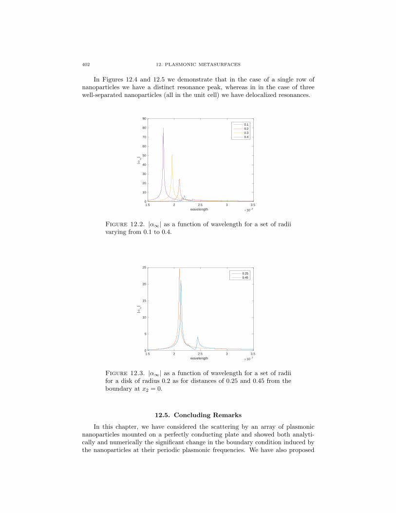
402 12. PLASMONIC METASURFACES
In Figures 12.4 and 12.5 we demonstrate that in the case of a single row ofnanoparticles we have a distinct resonance peak, whereas in in the case of threewell-separated nanoparticles (all in the unit cell) we have delocalized resonances.
1.5 2 2.5 3 3.5wavelength #10 -7
0
10
20
30
40
50
60
70
80
90
|,1
|
0.10.20.30.4
Figure 12.2. |α∞| as a function of wavelength for a set of radiivarying from 0.1 to 0.4.
1.5 2 2.5 3 3.5wavelength #10 -7
0
5
10
15
20
25
|,1
|
0.250.45
Figure 12.3. |α∞| as a function of wavelength for a set of radiifor a disk of radius 0.2 as for distances of 0.25 and 0.45 from theboundary at x2 = 0.
12.5. Concluding Remarks
In this chapter, we have considered the scattering by an array of plasmonicnanoparticles mounted on a perfectly conducting plate and showed both analyti-cally and numerically the significant change in the boundary condition induced bythe nanoparticles at their periodic plasmonic frequencies. We have also proposed

12.5. CONCLUDING REMARKS 403
1.5 2 2.5 3 3.5
wavelength #10 -7
0
10
20
30
40
50
60
70
|,1
|
-0.5 0 0.50
0.5
1
Figure 12.4. We observe a strong localized resonant peak in thecase of a single row of nanoparticles.
1.5 2 2.5 3 3.5wavelength #10 -7
0
0.5
1
1.5
2
2.5
3
3.5
4
4.5
5
|,1
|
-0.5 0 0.50
0.5
1
Figure 12.5. When we have three nanoparticles in each cell ofthe array we observe delocalized resonance.
an optimization approach to maximize this change in terms of the shape of thenanoparticles. Our results in this chapter can be generalized in many directions.Different boundary conditions on the plate as well as curved plates can be consid-ered. Our approach can be easily extended to two-dimensional arrays embedded inR3 and the lattice effect can be included by using the Green’s function for a generallattice (as in (2.128)). Full Maxwell’s equations to model the light propagation canbe used. The observed extraordinary or meta-properties of periodic distributionsof subwavelength resonators can be explained by the approach proposed in thischapter.


Part 5
Subwavelength Phononics

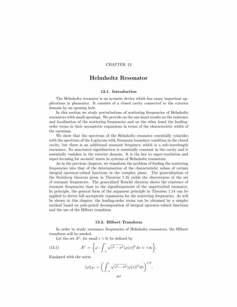
CHAPTER 13
Helmholtz Resonator
13.1. Introduction
The Helmholtz resonator is an acoustic device which has many important ap-plications in phononics. It consists of a closed cavity connected to the exteriordomain by an opening hole.
In this section we study perturbations of scattering frequencies of Helmholtzresonators with small openings. We provide on the one hand results on the existenceand localization of the scattering frequencies and on the other hand the leading-order terms in their asymptotic expansions in terms of the characteristic width ofthe openings.
We show that the spectrum of the Helmholtz resonator essentially coincideswith the spectrum of the Laplacian with Neumann boundary condition in the closedcavity, but there is an additional resonant frequency which is a sub-wavelengthresonance. Its associated eigenfunction is essentially constant in the cavity and itessentially vanishes in the exterior domain. It is the key to super-resolution andsuper-focusing for acoustic waves in systems of Helmholtz resonators.
As in the previous chapters, we transform the problem of finding the scatteringfrequencies into that of the determination of the characteristic values of certainintegral operator-valued functions in the complex plane. The generalization ofthe Steinberg theorem given in Theorem 1.16 yields the discreteness of the setof resonant frequencies. The generalized Rouche theorem shows the existence ofresonant frequencies close to the eigenfrequencies of the unperturbed resonator.In principle, the general form of the argument principle in Theorem 1.14 can beapplied to derive full asymptotic expansions for the scattering frequencies. As willbe shown in this chapter, the leading-order terms can be obtained by a simplermethod based on pole-pencil decomposition of integral operator-valued functionsand the use of the Hilbert transform.
13.2. Hilbert Transform
In order to study resonance frequencies of Helmholtz resonators, the Hilberttransform will be needed.
Let the set X ǫ, for small ǫ > 0, be defined by
(13.1) X ǫ =
ϕ :
∫ ǫ
−ǫ
√ǫ2 − x2 |ϕ(x)|2 dx < +∞
,
Equipped with the norm
‖ϕ‖X ǫ =
(∫ ǫ
−ǫ
√ǫ2 − x2 |ϕ(x)|2 dx
)1/2
,
407

408 13. HELMHOLTZ RESONATOR
X ǫ is a Hilbert space. Introduce
(13.2) Yǫ =
ψ ∈ C0 ( [−ǫ, ǫ ] ) : ψ′ ∈ X ǫ
,
where ψ′ is the distribution derivative of ψ. The set Yǫ is a Hilbert space with thenorm
‖ψ‖Yǫ =
(||ψ||2X ǫ + ||ψ′||2X ǫ
)1/2
.
Let Lǫ : X ǫ → Yǫ be defined by
(13.3) Lǫ[ϕ](x) =∫ ǫ
−ǫln |x− y|ϕ(y) dy.
We establish two results concerning the integral operator Lǫ. These results areproved in [422].
Lemma 13.1. For all 0 < ǫ < 2, the integral operator Lǫ : X ǫ 7→ Yǫ is invertible.Let ϕ be a function of X ǫ. The function
ψ(x) =
∫ ǫ
−ǫln |x− y| ϕ(y) dy
is differentiable and its derivative on (−ǫ, ǫ) is given by (see for instance [368, p.30])
(13.4) ψ′(x) = Hǫ[ϕ](x),
where Hǫ denotes the finite Hilbert transform (or Tricomi’s operator)
(13.5) Hǫ[ϕ](x) =
∫ ǫ
−ǫ
ϕ(y)
x− ydy for x ∈ (−ǫ, ǫ) .
The following explicit expressions hold. For any x ∈ (−ǫ, ǫ) , we have
(13.6) Hǫ[1√
ǫ2 − y2](x) = 0,
(13.7) Hǫ[√ǫ2 − y2](x) = πx,
and
(13.8) Hǫ[y√
ǫ2 − y2](x) = −π.
The main difficulty in studying the finite Hilbert transform Hǫ on Holder con-tinuous functions (with requirements at the endpoints) is that it has no smoothnesspreserving property, as shown by the following formulas:
Hǫ[1](x) = lnǫ+ x
ǫ− x
and
H′ǫ[ϕ](x)−
ϕ(−ǫ)ǫ+ x
+ϕ(ǫ)
ǫ− x+Hǫ[ϕ
′](x).
The development of such a theory is a rather long and complicated process. Seefor instance [380].
Here the weighted space X ǫ is introduced to make the theory relatively simpleand yet general enough for applications. The following mapping properties of thefinite Hilbert transform hold. See [422] for a proof.

13.2. HILBERT TRANSFORM 409
Lemma 13.2 (Finite Hilbert transform). The operator Hǫ : X ǫ → X ǫ satisfiesdimKer(Hǫ) = 1 and Im Hǫ = X ǫ.
As shown by formula (13.6), Ker(Hǫ) is spanned by 1/√ǫ2 − y2. We refer the
reader to [95, 206] for the mapping properties of the finite Hilbert transform inmore general weighted spaces. We will need the following Holder estimate [368]
(13.9)
∥∥∥∥∫ 1
−1
ϕ(y)
x− ydy
∥∥∥∥L∞([−1,1])
≤ C ‖ϕ‖C0,η([−1,1])
for ϕ ∈ C0,η([−1, 1]) with η > 0.We now solve explicitly the integral equation
(13.10) Lǫ[ϕ](x) = ψ(x), ∀ x ∈ (−ǫ, ǫ) ,where ψ is a given function in Yǫ and ϕ is the unknown function. Differentiating(13.10) with respect to the x-variable, we obtain the singular integral equation(13.4). The general solution of equation (13.4) is given by the Hilbert inversionformula (see for instance [368]):
(13.11) ϕλ(x) = − 1
π2√ǫ2 − x2
∫ ǫ
−ǫ
√ǫ2 − y2ψ′(y)
x− ydy +
λ√ǫ2 − x2
,
where λ is a complex constant. Therefore, the solution ϕ in X ǫ of (13.10) is neces-sarily one of the ϕλ given by (13.11), where λ is chosen appropriately. Denote byλ(ψ) the appropriate choice of λ and consider
(13.12) a(ψ) = ψ(x)− Lǫ[ϕλ=0](x).
We first observe that the quantity a(ψ) is a constant, since its derivative withrespect to x is identically equal to zero on (−ǫ, ǫ). Now, substitute ϕλ(ψ) into(13.10) to get
λ(ψ)Lǫ[y 7→ 1√
ǫ2 − y2
]= a(ψ).
But, a straightforward calculation shows that
Lǫ[y 7→ 1√
ǫ2 − y2
](x) = π ln
ǫ
2for all x ∈ (−ǫ, ǫ) ,
and therefore,
λ(ψ) =a(ψ)
π ln(ǫ/2).
Thus,(13.13)
L−1ǫ [ψ](x) = − 1
π2√ǫ2 − x2
∫ ǫ
−ǫ
√ǫ2 − y2ψ′(y)
x− ydy +
a(ψ)
(π ln(ǫ/2))√ǫ2 − x2
,
where a(ψ) is given by (13.12). This calculation has been done by Carleman in[169].
Note that for ǫ = 2, L2 has a nontrivial kernel. However, for 0 < ǫ < 2, thesolution to (13.10) is clearly unique. In fact, by (13.11) and (13.12), it follows thatif ψ ≡ 0, then L−1
ǫ [ψ] ≡ 0.
We will also need the following lemma.

410 13. HELMHOLTZ RESONATOR
Lemma 13.3. Let Rǫ be the integral operator defined from X ǫ into Yǫ by
Rǫ[ϕ](x) =
∫ ǫ
−ǫR(x, y)ϕ(y) dy,
with R(x, y) of class C1,η in x and y, for η > 0. There exists a positive constant C,independent of ǫ, such that
(13.14) ‖L−1ǫ Rǫ‖L(X ǫ,X ǫ) ≤
C
| ln ǫ| ,
where
‖L−1ǫ Rǫ‖L(X ǫ,X ǫ) = sup
ϕ∈X ǫ,‖ϕ‖Xǫ=1
‖L−1ǫ Rǫ[ϕ]‖X ǫ .
Proof. Let ϕ ∈ X ǫ. By the Hilbert inversion formula (13.11), we have
L−1ǫ Rǫ[ϕ](x) = − 1
π2√ǫ2 − x2
∫ ǫ
−ǫ
√ǫ2 − y2(Rǫ[ϕ])
′(y)
x− ydy +
λ(Rǫ[ϕ])√ǫ2 − x2
(13.15)
: = Iǫ1[ϕ](x) + Iǫ2[ϕ](x),
where
λ(Rǫ[ϕ]) =a(Rǫ[ϕ])
π ln(ǫ/2).
We estimate ‖Iǫ1[ϕ]‖X ǫ and ‖Iǫ2[ϕ]‖X ǫ separately.For ‖Iǫ1[ϕ]‖X ǫ , we have
‖Iǫ1[ϕ]‖X ǫ
∫ ǫ
−ǫ
1√ǫ2 − x2
(∫ ǫ
−ǫ
√ǫ2 − y2 (Rǫ[ϕ])
′(y)
x− ydy
)2
dx
12
≤ C
∥∥∥∥∥
∫ ǫ
−ǫ
√ǫ2 − y2 (Rǫ[ϕ])
′(y)
x− ydy
∥∥∥∥∥L∞([−ǫ,ǫ])
= Cǫ
∥∥∥∥∥
∫ 1
−1
√1− y2 (Rǫ[ϕ])
′(ǫy)
x− ydy
∥∥∥∥∥L∞([−1,1])
.
We then have from the Holder estimate (13.9) for the Hilbert transform∥∥∥∥∥
∫ 1
−1
√1− y2 (Rǫ[ϕ])
′(ǫy)
x− ydy
∥∥∥∥∥L∞([−1,1])
≤ C∥∥∥√1− y2 (Rǫ[ϕ])
′(ǫy)∥∥∥C0,η([−1,1])
≤ C ‖(Rǫ[ϕ])′(ǫy)‖C0,η([−1,1])
≤ C ‖(Rǫ[ϕ])′(y)‖C0,η([−ǫ,ǫ])
≤ C
∫ ǫ
−ǫ|ϕ(y)| dy ≤ C‖ϕ‖X ǫ ,
since the kernel R is of class C1,η. Thus, we obtain
(13.16) ‖Iǫ1[ϕ]‖X ǫ ≤ Cǫ‖ϕ‖X ǫ .

13.2. HILBERT TRANSFORM 411
To estimate ‖Iǫ2[ϕ]‖X ǫ , we first observe that
‖Iǫ2[ϕ]‖X ǫ =
(∫ ǫ
−ǫ
√ǫ2 − x2|Iǫ2[ϕ](x)|2dx
)1/2
=√π|λ(Rǫ[ϕ])| =
∣∣∣∣a(Rǫ[ϕ])√π ln(ǫ/2)
∣∣∣∣ .
At this point, let us recall that
a(Rǫ[ϕ]) = Rǫ[ϕ]− Lǫ[t 7→ 1√
ǫ2 − t2
∫ ǫ
−ǫ
√ǫ2 − y2
t− y(Rǫ[ϕ])
′(y) dy
].
Once again, from the smoothness of the kernel R in x and y, we have
(13.17) sup−ǫ≤x≤ǫ
|Rǫ[ϕ](x)| ≤ C ‖ϕ‖X ǫ .
On the other hand, we get from (13.7) that∫ ǫ
−ǫ
√ǫ2 − y2
t− y(Rǫ[ϕ])
′(y) dy
= (Rǫ[ϕ])′(t)
∫ ǫ
−ǫ
√ǫ2 − y2
t− ydy +
∫ ǫ
−ǫ
√ǫ2 − y2
t− y[(Rǫ[ϕ])
′(y)− (Rǫ[ϕ])′(t)] dy
= πt(Rǫ[ϕ])′(t) +
∫ ǫ
−ǫ
√ǫ2 − y2
t− y[(Rǫ[ϕ])
′(y)− (Rǫ[ϕ])′(t)] dy.
Put
Iǫ(t) :=
∫ ǫ
−ǫ
√ǫ2 − y2
t− y[(Rǫ[ϕ])
′(y)− (Rǫ[ϕ])′(t)] dy.
Then, we have
|Iǫ(t)| ≤ Cǫ1+η supt,y
∣∣∣∣(Rǫ[ϕ])
′(y)− (Rǫ[ϕ])′(t)
|y − t|η∣∣∣∣
≤ Cǫ1+η∫ ǫ
−ǫ|ϕ(y)|dy ≤ Cǫ1+η‖ϕ‖X ǫ .
Therefore, it follows that∣∣∣∣∣Lǫ[t 7→ 1√
ǫ2 − t2
∫ ǫ
−ǫ
√ǫ2 − y2
t− y(Rǫ[ϕ])
′(y) dy
]∣∣∣∣∣
≤∣∣∣∣Lǫ[πt(Rǫ[ϕ])
′(t)√ǫ2 − t2
]∣∣∣∣+∣∣∣∣Lǫ[
Iǫ(t)√ǫ2 − t2
]∣∣∣∣
≤(supt
|πt(Rǫ[ϕ])′(t)|+ sup
t|Iǫ(t)|
) ∣∣∣∣Lǫ[
1√ǫ2 − t2
]∣∣∣∣ ≤ Cǫ| ln ǫ|‖ϕ‖X ǫ ,
which, combined with (13.17), gives
(13.18) ‖Iǫ2[ϕ]‖X ǫ ≤ C
| ln ǫ| ‖ϕ‖X ǫ .
Combining (13.16) and (13.18) yields the desired estimate (13.14).

412 13. HELMHOLTZ RESONATOR
13.3. Perturbations of Scattering Frequencies of a Helmholtz Resonator
Let Ω ⊂ R2 be a bounded simply connected domain with boundary ∂Ω of classC2. Let µ0 be a simple eigenvalues of −∆ in Ω with Neumann conditions, namely, asimple eigenvalue of (3.1) and let V be a neighborhood of µ0 in the complex planesuch that µ0 is the only eigenvalue of (3.1) in V .
The acoustic Helmholtz resonator we consider is a surface ∂Ωǫ = ∂Ω \ Σǫ,where ∂Ωǫ is obtained from ∂Ω by making a small opening Σǫ in the boundarywith diameter tending to zero as ǫ→ 0. This opening connects the interior and theexterior parts of the resonator. If µ0 is an eigenvalue of (3.1), the correspondingscattering problem is to find µǫ (with ℑmµǫ ≥ 0) close to µ0 such that there existsa nontrivial solution to
(13.19)
(∆ + µǫ)uǫ = 0 in Ω ∪ (R2 \ Ω),∂uǫ
∂ν= 0 on ∂Ωǫ,∣∣∣∣
∂uǫ
∂r−√
−1µǫuǫ∣∣∣∣ = O(r−1) as r = |x| → +∞.
As in the previous chapters, we reduce the scattering problem (13.19) to thestudy of characteristic values of a certain operator-valued function, and by meansof the generalized Rouche theorem we prove the existence of a scattering frequencyµǫ with small imaginary part which converges to µ0 as ǫ → 0. We then constructthe leading-order term in its asymptotic expansion.
To simplify the exposition, we shall assume that 0 is the center to which theopening can be contracted and the opening Σǫ is flat: Σǫ = (−ǫ, ǫ). It can be shownthat the curvature of the opening does not influence the leading-order term in theasymptotic expansion of the scattering frequencies [227]. Following the argumentspresented in the previous section, we only outline the derivation of an asymptoticexpansion of µǫ, leaving the details to the reader.
13.3.1. Problem Formulation. We say that µ ∈ C (with ℑmµ ≥ 0) is ascattering pole if there exists a nontrivial solution to the exterior problem
(13.20)
(∆ + µ)v = 0 in R2 \ Ω,∂v
∂ν= 0 on ∂Ω,
∫
R2\Ω|v|2 < +∞.
Introduce the exterior Neumann function Nõ
R2\Ω, that is, the unique solution
to
(13.21)
(∆x + µ)N√µ
R2\Ω(x, z) = −δz in R2 \ Ω,∂N
õ
R2\Ω∂ν
∣∣∣∂Ω
= 0 on ∂Ω,
∣∣∣∣∂N
õ
R2\Ω∂r
−√−1µN
õ
R2\Ω
∣∣∣∣ = O(r−1) as r = |x| → +∞.

13.3. PERTURBATIONS OF SCATTERING FREQUENCIES 413
Set ϕǫ to be the normal derivative of uǫ on the opening Σǫ:
ϕǫ =∂uǫ
∂νon Σǫ.
By Green’s formula, ϕǫ satisfies the integral equation
(13.22)
∫
Σǫ
(N
√µǫ
R2\Ω +N√µǫ
Ω
)(x, y)ϕǫ(y) dy = 0 on Σǫ,
where the interior Neumann function N√µǫ
Ω is defined by (2.179) and the exterior
Neumann function N√µǫ
R2\Ω is defined by (13.21).
Define the operator-valued function µ 7→ Aǫ(µ) by
Aǫ(µ)[ϕ](x) :=
∫ ǫ
−ǫ
(N
√µǫ
R2\Ω +N√µǫ
Ω
)(x, y)ϕ(y) dy.
By virtue of (13.22), the problem of finding the scattering frequencies can bereduced to that of finding the characteristic values of Aǫ(µ).
13.3.2. Asymptotic Formula for Perturbations in Scattering Frequen-cies. Let µ0 be a simple eigenvalue of (3.1) associated with the normalized eigen-function uj0 and let V be a complex neighborhood of µ0 such that (i) µ0 is the onlyeigenvalue of (3.1) in V and (ii) there is no scattering pole of (13.20) in V .
Writing
Nõ
R2\Ω(x, z) = − 1
2πln |x− z|+ r(x, z, µ),
where r(x, z, µ) is holomorphic with respect to µ in V and smooth in x and z, weobtain the following pole-pencil decomposition of Aǫ in V .
Lemma 13.4. The following pole-pencil decomposition of Aǫ(µ) : X ǫ → Yǫholds for any µ ∈ V \ µ0:
(13.23) Aǫ(µ) = − 1
πLǫ +
Kǫµ0 − µ
+Rǫ(µ),
where
Lǫ[ϕ](x) =∫ ǫ
−ǫln |x− y|ϕ(y) dy,
Kǫ is the one-dimensional operator given by
Kǫ[ϕ](x) = 〈ϕ, uj0〉L2(Σǫ) uj0 ,
and
Rǫ(µ)[ϕ](x) =
∫ ǫ
−ǫR(µ, x, y)ϕ(y) dy,
with (µ, x, y) 7→ R(µ, x, y) holomorphic in µ and smooth in x and y.
We now prove that the set of characteristic values of Aǫ is discrete.
Lemma 13.5. The set of characteristic values of µ 7→ Aǫ(µ) is discrete.
Proof. We only give a proof for the discreteness of the set of characteristicvalues of Aǫ in V . The same arguments apply in neighborhoods Vj of µj , j ≥ 1,and in C \⋃j Vj . Recall that Lǫ : X ǫ → Yǫ is invertible and ‖L−1
ǫ Rǫ‖L(X ǫ,X ǫ) →0 as ǫ → 0. Therefore, −(1/(π))Lǫ + Rǫ : X ǫ → Yǫ is invertible for ǫ smallenough. It then follows from the pole-pencil decomposition (13.23) that Aǫ is

414 13. HELMHOLTZ RESONATOR
finitely meromorphic and of Fredholm type in V . Moreover, since Kǫ is of finite-dimension, there exists µ∗ ∈ V such that Aǫ(µ
∗) is invertible. Therefore, thegeneralization of the Steinberg theorem (Theorem 1.16) gives the discreteness ofthe set of characteristic values of Aǫ in V .
Next, we prove that there exists exactly one characteristic value of Aǫ locatedin the neighborhood V of µ0 and compute its asymptotic expansion as ǫ goes tozero. The method is based on the pole-pencil decomposition (13.23) of the operator-valued function Aǫ, followed by an application of the generalized Rouche theorem.
Lemma 13.6. The operator-valued function Aǫ(µ) has exactly one characteristicvalue in V .
Proof. We first study the principal part of Aǫ, that is, the integral operator-valued function defined by
Nǫ : µ 7→ Nǫ(µ) = − 1
πLǫ +
Kǫµ0 − µ
,
and show that its multiplicity in V is equal to zero. Let us find the characteristicvalues of Nǫ in V , that is, the complex numbers µ, such that there exists ϕ 6≡ 0satisfying Nǫ(µ)[ϕ] ≡ 0 on (−ǫ, ǫ). Equivalently, we have
1
πLǫ[ϕ] +
〈ϕ, uj0〉µ− µ0
uj0 = 0.
Since the operator Lǫ is invertible, it follows that
(13.24)1
πϕ+
〈ϕ, uj0〉µ− µ0
L−1ǫ [uj0 ] = 0,
and, by multiplying (13.24) by uj0 , we find
〈ϕ, uj0〉(1
π+
〈L−1ǫ [uj0 ], uj0〉µ− µ0
)= 0.
Hence,
(13.25) µ = µ0 − π〈L−1ǫ [uj0 ], uj0〉,
since by (13.24), 〈ϕ, uj0〉 = 0 would imply that ϕ ≡ 0.Moreover, from
|〈L−1ǫ [uj0 ], uj0〉| −→ 0 as ǫ→ 0,
it follows that
|µ− µ0| −→ 0 as ǫ→ 0.
If the normalization condition 〈ϕ, uj0〉 = 1 is chosen, then (13.24) and (13.25) showthat the root function associated to this characteristic value µ is given by
ϕ =L−1ǫ [uj0 ]
〈L−1ǫ [uj0 ], uj0〉
.
The last point to investigate is the multiplicity of µ as a characteristic value ofNǫ, that is, the order of µ as a pole of N−1
ǫ . A straightforward calculation showsthat Nǫ(µ)[ϕ] = f is equivalent to
− 1
πϕ+
〈ϕ, uj0〉L−1ǫ [uj0 ]
µ0 − µ= L−1
ǫ [f ].

13.3. PERTURBATIONS OF SCATTERING FREQUENCIES 415
But
〈ϕ, uj0〉[− 1
π+
〈L−1ǫ [uj0 ], uj0〉µ0 − µ
]= 〈L−1
ǫ [f ], uj0〉,
which yields
〈ϕ, uj0〉 =π(µ0 − µ)
µ− µ〈L−1
ǫ [f ], uj0〉,and therefore,(13.26)
Nǫ(µ)[ϕ] = f if and only if ϕ = −πL−1ǫ [f ] +
π2〈L−1ǫ [f ], uj0〉µ− µ
L−1ǫ [uj0 ],
which justifies that µ is a characteristic value of order one of Nǫ. Therefore, Nǫ hasexactly one pole µ0 and one characteristic value µ in V , each of order one, and itsfull multiplicity is equal to zero.
Now we estimate the multiplicity of Aǫ in V . The function µ 7→ Nǫ(µ) is clearlyfinitely meromorphic and of Fredholm type at µ = µ0. For all µ ∈ V \ µ0, µ,Nǫ is invertible. Thus, Nǫ is normal in V . Moreover, Aǫ(µ) − Nǫ(µ) = Rǫ(µ) isanalytic in V and, by (13.26), it satisfies
limǫ→0
‖N−1ǫ (µ)Rǫ(µ)‖L(X ǫ,X ǫ) = 0, ∀ µ ∈ ∂V.
Consequently, the integral operator-valued function µ 7→ Aǫ(µ) has, by the gen-eralized Rouche theorem, the same full multiplicity as Nǫ in V . Since it alreadyadmits µ0 as a pole, it admits in this neighborhood exactly one characteristic valueµǫ.
Now in view of Lemmas 13.4 and 13.6, we obtain the following theorem.
Theorem 13.7. The operator-valued function Aǫ(µ) has exactly one charac-teristic value µǫ in V . Moreover, the following asymptotic expansion of µǫ holds:
(13.27) µǫ ≈ µ0 − π〈L−1ǫ [uj0 ], uj0〉+ π2〈L−1
ǫ Rǫ(µ0)L−1ǫ [uj0 ], uj0〉,
which yields
µǫ ≈ µ0 −π
ln ǫ|uj0(0)|2.
Proof. Recall that if µǫ is the eigenvalue of (13.19) in V , then it is the char-acteristic value of Aǫ in V . Let ϕǫ be an associated root function to µǫ. SinceI + L−1
ǫ Rǫ is invertible for ǫ small enough, one can see as in the proof of Lemma13.6 that 〈ϕǫ, uj0〉 6= 0, and hence we can choose ϕǫ such that 〈ϕǫ, uj0〉 = 1. Withthis choice, we have
(13.28)1
2π+
〈L−1ǫ [uj0 ], uj0〉µǫ − µ0
− 〈L−1ǫ Rǫ(µ
ǫ)[ϕǫ], uj0〉 = 0,
from which it follows by using (13.14) that
µǫ = µ0 − 2π〈L−1ǫ [uj0 ], uj0〉+O(| ln ǫ|−2).
But,
(− 1
2πI + L−1
ǫ Rǫ(µǫ))[ϕǫ] +
L−1ǫ [uj0 ]
µ0 − µǫ= 0,
and thus,
ϕǫ ≈ L−1ǫ [uj0 ]
〈L−1ǫ [uj0 ], uj0〉
.

416 13. HELMHOLTZ RESONATOR
Inserting the above approximation of ϕǫ into (13.28) yields (13.27), as desired.
Theorem 13.7 shows in particular the existence of a sub-wavelength resonancefor the Helmholtz resonator Ωǫ and lets us determine its asymptotic expansion interms of the size ǫ of the opening. Choose µ0 = 0 (with the associated eigenfunction
= 1/√|Ω| in Ω). It follows that there exists a unique characteristic value µǫ of Aǫ
in a small neighborhood of 0. Moreover,
(13.29) µǫ ≈ − π
|Ω| ln ǫ .
In the three-dimensional case, we can prove that [83]
(13.30) µǫ ≈ 1
|Ω|ǫcap(Σ),
where
(13.31) cap(Σ) := −〈L−11 [1], 1〉L2(Σ)
is the capacity of Σ := Σǫ in the rescaled opening (of arbitrary smooth shape) andL1 is the three-dimensional analog to Lǫ defined by (13.3) with ǫ = 1:
L1 : ϕ 7→ 1
π
∫
Σ
ϕ(y)
|x− y|dy, x ∈ R3\Σ.
We refer to formulas (13.29) and (13.30) as the frequency formula for respec-tively the two and three-dimensional Helmholtz resonator. Formulas (13.29) and(13.30) indicate that it is possible to construct acoustic resonant structures thatare much smaller than the wavelength of the corresponding acoustic wave. Fur-thermore, the frequency formulas can be generalized to a system of L disjointHelmholtz resonators separated by a distance of the order of their characteristicsize. It was shown in [83] that L (counting multiplicity) sub-wavelength resonancesdo exist and their asymptotic expansions as the characteristic size of the openingsgoes to zero were derived. Note that the term “sub-wavelength resonator” is as-sociated with scattering in the quasi-stationary regime. In fact, in the case of theHelmholtz resonator, it is in that regime that the free space wavelength is signifi-cantly greater than the size of the resonator. We also remark that the resonance inthe quasi-stationary regime results from the perturbations of the zero-eigenvalue ofthe Neumann problem in the closed resonator that are due to small openings. Inthe next subsection, we briefly outline the frequency formula and its consequenceon super-resolution.
13.4. Resonances of a System of Helmholtz Resonators andSuper-Resolution
Let the single three-dimensional Helmholtz resonator Ω be such that Ω =S(0, 1) × [−h, 0], where S(0, 1) = (x1, x2) : x21 + x22 ≤ 1 and h is the heightof Ω, which is of order one. Let Σ ⊂ S(0, 1) ⊂ R2 be a simply connected smoothdomain which is of size one and let ǫ > 0 be a small number. We assume that 0 ∈ Σwithout loss of generality.
Consider a system of such resonators in three dimensions which consists of L
disjoint Ωj ’s (1 ≤ j ≤ L), where Ωj = Ω + z(j) and z(j) = (z(j)1 , z
(j)2 , 0) is the
center of the opening for jth resonator. We denote by Ωin =⋃Lj=1 Ωj , Ωex =
(x1, x2, x3) ∈ R3 : x3 > 0 and Ωǫ = Ωin⋃Ωex
⋃Σǫ with Σǫ =
⋃Lj=1 Σǫ,j .

13.4. HELMHOLTZ RESONATORS AND SUPER-RESOLUTION 417
We first introduce two auxiliary Green’s functions. Let Nex be the Greenfunction for the following exterior scattering problem:
(∆ + ω2)Nexω (x, y) = δy(x), x ∈ Ωex,
∂Nexω
∂ν (x, y) = 0, x ∈ ∂Ωex,Nexω satisfies the Sommerfeld radiation condition,
and N inω be the Green function for the following interior problem:
(∆ + ω2)N in
ω (x, y) = δy(x), x ∈ Ω,∂Nin
ω
∂ν (x, y) = 0, x ∈ ∂Ω.
Throughout this section, we denote by
W = ω ∈ C : |ω| ≤ 1
2
õ2,
where µ2 is the first nonzero eigenvalue of the Neumann problem in Ω (µ1 = 0).We have the following result.
Lemma 13.8. Let y ∈ x3 = 0 and ω ∈W . Then,
Nexω (x, y) =
1
2π|x− y| +Rex(x, y, ω), x ∈ Ωex,(13.32)
N inω (x, y) =
1
2π|x− y| −ψ(x)ψ(y)
ω2+Rin(x, y, ω), x ∈ Ω,(13.33)
where ψ = χ(Ω) and
Rex(x, y, ω) =
√−1ω
2π
∫ 1
0
e√−1ω|x−y|tdt,
Rin(x, y, ω) = ω
∫ 1
0
sin√−1ω|x− y|tdt+ r(x, y, ω)
for some function r which is analytic in W with respect to ω and is smooth in aneighborhood of Σ in the plane x3 = 0 with respect to both the variables x and y.
We denote by
R(x, y, ω) = Rex(x, y, ω) +Rin(x, y, ω),
and
(13.34) α0 = R(0, 0, 0), α1 =∂R
∂ω(0, 0, 0).
It is clear that
(13.35) α0 ∈ R, ℑα1 = ℑ∂Rex
∂ω(0, 0, 0) =
1
2π.
We now introduce the matrices T = (Tij)L×L and S = (Sij)L×L with
(13.36)
Tij = 1
2π|z(i)−z(j)| for i 6= j, and Tii = 0,
Sij =√−12π + δijℜα1.
Observe that T is symmetric, thus T has L real eigenvalues, which are denotedby β1, β2, . . . , βL. For the ease of exposition, we assume that β1, . . . , βL are mutually distinct.This is the generic case among all the possible arrangements of the resonators. The

418 13. HELMHOLTZ RESONATOR
corresponding normalized eigenvectors are denoted by Y1, Y2, . . . , YL, respectively.Then Y1, Y2, . . . , YL form a normal basis for RL. We also denote by Y the matrix
Y = (Y1, Y2, . . . , YL).
For convenience, we write
(13.37) N (x,ω) =(Nexω (x, z(1)), Nex
ω (x, z(2)), . . . , Nexω (x, z(L))
)t
with the subscript t denoting the transpose. For each 1 ≤ j ≤ L, we denote by
(13.38) ζj(x, x0, ω) = N (x, ω)tYjYtjN (x0, ω).
It is clear that ζj = ζj(x, x0, ω) is analytic in ω for fixed x and x0.The following result on the resonances of the above scattering problem was
proved in [83].
Proposition 13.9. There exist exactly 2L resonances of order one in the do-main W for the system of resonators, given by
ω0,ǫ,j,1 = τ1ǫ12 + τ3,jǫ
32 + τ4,jǫ
2 +O(ǫ52 ),(13.39)
ω0,ǫ,j,2 = −τ1ǫ12 − τ3,jǫ
32 + τ4,jη
2 +O(ǫ52 ),(13.40)
where
(13.41) τ1 =
√cap(Σ)
|Ω| ,
(13.42) τ3,j = −1
2(α0 + βj)
(cap(Σ)
|Ω|
) 12
cap(Σ),
and
(13.43) τ4,j = −1
2
cap(Σ)2
|Ω| Y tj SYj
with cap(Σ) being the capacity of the set Σ defined by (13.31).
From Chapter 9, the super-resolution relies in analysis of the following Greenfunction in the frequency domain
(∆ + ω2)Nǫ(x, x0, ω) = δx0(x), x ∈ Ωǫ,
∂Nǫ
∂ν (x, x0, ω) = 0, x ∈ ∂Ωǫ,
Nǫsatisfies the Sommerfeld radiation condition.
The following result on Nǫ in Ωǫ holds. We refer to [83] for its proof.
Theorem 13.10. Assume that ω ∈ R⋂W . Then for ǫ sufficiently small. Then
Nexǫ has the following asymptotic expansion
Nexǫ (x, x0, ω) = Nex
ω (x, x0)− ǫcap(Σ)∑
1≤j≤LNexω (z(j), x0, k)N
exω (x, z(j))
−L∑
j=1
(1
ω − ω0,ǫ,j,2− 1
ω − ω0,ǫ,j,1
)(cap(Σ)ǫ)
32
√|D|
N (x, ω)tYjYtjN (x0, ω)
+∑
1≤j≤L
(O(ǫ2)
ω − ω0,ǫ,j,2+
O(ǫ2)
ω − ω0,ǫ,j,1
)+O(ǫ2).

13.5. CONCLUDING REMARKS 419
As a consequence of Theorem 13.10, we can establish the following resulton super-resolution (or super-focusing), which shows that super-resolution can beachieved with a single specific frequency.
Theorem 13.11. Let τ1 be given by (13.41), where cap(Σ) is the capacity ofthe set Σ defined by (13.31). For ω = τ1
√ǫ, the resolution function ℑNex
ǫ has thefollowing estimate:
ℑNexǫ (x, x0, ω) =
sin τ1√ǫ|x− x0|
2π|x− x0|+
cap(Σ)32
|Ω| 12ǫ
12
L∑
j=1
ℑτ4,jτ23,j
ζj(x, x0, 0) +O(ǫ),
where ζj(x, x0, 0) is given by (13.38) and τ3,j and τ4,j are defined by (13.42) and(13.43), respectively.
13.5. Concluding Remarks
In this chapter, we have derived asymptotic expansions of perturbations ofscattering frequencies of sub-wavelength acoustic resonators. As in the previouschapters, we have transformed the problem of finding the scattering frequencies intothe determination of the characteristic values of certain integral operator-valuedfunctions in the complex plane. Our method in this chapter is based on pole-penciltype decomposition, followed by an application of the generalized Rouche theorem.The techniques developed in this chapter can be extended to electromagnetic andelastic analogues of the Helmholtz resonator [229, 232, 377, 215].


CHAPTER 14
Minnaert Resonances for Bubbles
14.1. Introduction
In this chapter, we consider acoustic wave propagation in bubbly media. Atparticular low frequencies known as Minnaert resonances [359], bubbles behave asstrong sound scatterers. Using layer potential techniques and Gohberg-Sigal theory,we first derive a formula for the Minnaert resonances of bubbles of arbitrary shapes.The Minnaert resonance is a low frequency resonance in which the wavelength ismuch larger than the size of the bubble. Our formula for the Minnaert resonanceis expressed in terms of the bulk modulus of the air, the density of the water, andthe capacity and the volume of the bubbles.
Then, we derive an effective medium theory for acoustic wave propagation inbubbly media near the Minnaert resonant frequency. We consider the dilute regime.We start with a multiple scattering formulation of the scattering problem in whichan incident wave impinges on a large number of identical and small bubbles in ahomogeneous fluid. Under certain conditions on the configuration of the bubblesdistribution, we justify the point interaction approximation and establish an effec-tive medium theory for the bubbly fluid as the number of bubbles tends to infinity.The convergence rate is also derived. As a consequence, we show that near andbelow the Minnaert resonant frequency, the obtained effective media may be highlyrefractive, making the superfocusing of acoustic waves achievable.
On the other hand, we show that a subwavelength bandgap opening may oc-cur in bubble phononic crystals. To demonstrate the opening of a subwavelengthphononic bandgap, we consider a periodic arrangement of bubbles and exploit theirMinnaert resonance. As shown in Chapter 5, for bandgaps to occur, the period ofthe structure must be of the order of the wavelength and the contrast in the materialparameters must be large. This limits the use of phononic crystals in applicationstargeting low frequencies, because phononic crystals would require impracticallylarge geometries [343, 448]. In this chapter, we provide a mathematical and nu-merical framework for analyzing bandgap opening in bubble phononic crystals atlow-frequencies. We derive a formula for the quasi-periodic Minnaert resonancefrequencies of an arbitrarily shaped bubble, along with proving the existence of asubwavelength bandgap. In the dilute regime, above the Minnaert resonant fre-quency, the real part of the effective modulus is negative and consequently, thebubbly fluid behaves as a diffusive media for the acoustic waves.
We remark that such behavior near the resonant frequency is rather analogousto the coupling of electromagnetic waves with plasmonic nanoparticles, which re-sults in effective negative or high contrast dielectric constants for frequencies nearthe plasmonic resonance frequencies as shown in Chapter 7.
421
422 14. MINNAERT RESONANCES FOR BUBBLES
The results of this chapter, which are from [35, 36, 37], formally explain theexperimental observations reported in [314, 323, 325].
14.2. Derivation of Minnaert Resonance Formula
We consider the scattering of acoustic waves in a homogeneous three-dimensionalacoustic medium by a bubble embedded inside. Assume that the bubble occupiesa bounded and simply connected domain D with ∂D ∈ C1,η for some η > 0. Wedenote by ρb and κb the density and the bulk modulus of the air inside the bubble,respectively. We let ρ and κ be the corresponding parameters for the backgroundmedia R3\D.
Let ui be an incident plane wave. The scattering problem can be modeled bythe following equations:
(14.1)
∇ · 1ρ∇u+
ω2
κu = 0 in R3\D,
∇ · 1
ρb∇u+
ω2
κbu = 0 in D,
u+ − u− = 0 on ∂D,
1
ρ
∂u
∂ν
∣∣∣∣+
− 1
ρb
∂u
∂ν
∣∣∣∣−= 0 on ∂D,
u− ui satisfies the Sommerfeld radiation condition.
We introduce four auxiliary parameters to facilitate our analysis:
(14.2) v =
√ρ
κ, vb =
√ρbκb, k = ωv, kb = ωvb.
We also introduce two dimensionless contrast parameters:
(14.3) δ =ρbρ, τ =
kbk
=vbv
=
√ρbκ
ρκb.
By choosing appropriate physical units, we may assume that the bubble sizeis of order one and that the wave speeds outside and inside the bubble are bothof order one. Thus the contrast between the wave speeds is not significant. Weassume, however, that there is a large contrast in the bulk modulii. In summary,we assume that
(14.4) δ ≪ 1 and τ = O(1).
Then the solution u can be written as
(14.5) u(x) =
ui + SkD[ψ], x ∈ R3\D,SkbD [ψb], x ∈ D,
for some surface potentials ψ, ψb ∈ L2(∂D). Using the jump relations for the singlelayer potentials, it is easy to derive that ψ and ψb satisfy the following system ofboundary integral equations:
(14.6) A(ω, δ)[Ψ] = F,
where
A(ω, δ) =
(SkbD −SkD
− 12I + (KkbD )∗ −δ( 12I + (KkD)∗)
), Ψ =
(ψbψ
), F =
(ui
δ ∂ui
∂ν
).
14.2. DERIVATION OF MINNAERT RESONANCE FORMULA 423
One can show that the scattering problem (14.1) is equivalent to the system ofboundary integral equations (14.6).
It is clear thatA(ω, δ) is a bounded linear operator fromH := L2(∂D)×L2(∂D)to H1 := H1(∂D)× L2(∂D), i.e., A(ω, δ) ∈ L(H,H1).
The resonance of the bubble in the scattering problem (14.1) can be defined asall the complex numbers ω with positive imaginary part such that there exists anontrivial solution to the following equation:
(14.7) A(ω, δ)[Ψ] = 0.
These can be viewed as the characteristic values of the operator-valued analyticfunction (with respect to ω) A(ω, δ). We are interested in the quasi-static resonanceof the bubble, that is, the resonance frequency at which the size of the bubble ismuch smaller than the wavelength of the incident wave outside the bubble. Insome physics literature, this resonance is called the Minnaert resonance. Due toour assumptions on the bubble being of size order one, and the wave speed outside ofthe bubble also being of order one, this resonance should lie in a small neighborhoodof the origin in the complex plane. In what follows, we apply the Gohberg-Sigaltheory to find this resonance.
We first look at the limiting case when δ = ω = 0. It is clear that
(14.8) A0 := A(0, 0) =
(S0D −S0
D
− 12I + (K0
D)∗ 0
),
where S0D and (K0
D)∗ are respectively the single layer potential and the Neumann–
Poincare operator on ∂D associated with the Laplacian.Let A∗
0 be the adjoint of A.
Lemma 14.1. We have
(i) Ker(A0) = Im Ψ0 where Im Ψ0 denotes the space spanned by Ψ0 and
Ψ0 = α0
(ψ0
ψ0
)
with ψ0 = (S0D)
−1[1] and the constant α0 being chosen such that ‖Ψ0‖ = 1;(ii) Ker(A∗
0) = Im Φ0 where
Φ0 = β0
(0φ0
)
with φ0 = 1 on ∂D and the constant β0 being chosen such that ‖Φ0‖ = 1.
The above lemma shows that ω = 0 is a characteristic value for the operator-valued analytic function A(ω, δ). By the Gohberg-Sigal theory, we can concludethe following result about the existence of the quasi-static resonance.
Lemma 14.2. For any δ, sufficiently small, there exists a characteristic valueω0 = ω0(δ) to the operator-valued analytic function A(ω, δ) such that ω0(0) = 0and ω0 depends on δ continuously. This characteristic value is also the quasi-staticresonance (or Minnaert resonance).
We next perform asymptotic analysis on the operator A(ω, δ). With the samenotation as in Subsection 2.8.3.1, the following result holds.

424 14. MINNAERT RESONANCES FOR BUBBLES
Lemma 14.3. In the space L(H,H1), we have
A(ω, δ) := A0+B(ω, δ) = A0+ωA1,0+ω2A2,0+ω
3A3,0+δA0,1+δω2A2,1+O(ω4)+O(δω3),
where
A1,0 =
(τvSD,1 −vSD,1
0 0
), A2,0 =
(τ2v2SD,2 −v2SD,2τ2v2KD,2 0
), A3,0 =
(τ3v3SD,3 −v3SD,3τ3v3KD,3 0
),
A0,1 =
(0 00 −( 12I + (K0
D)∗)
), A2,1 =
(0 00 −v2KD,2
).
We define a projection P0 : H → H1 by
P0[Ψ] := 〈Ψ,Ψ0〉HΦ0,
and denote by
A0 = A0 + P0.
The following results hold.
Lemma 14.4. We have
(i) The operator A0 is a bijective operator in L(H1,H). Moreover, A0[Ψ0] =Φ0;
(ii) The adjoint of A0, A0
∗, is a bijective operator in L(H,H1). Moreover,
A0
∗[Φ0] = Ψ0.
Proof. By construction, and the fact that S0D is bijective from L2(∂D) to
H1(∂D) in three dimensions, we can show that A0 is a bijective. So too is A0
∗. We
only need to show that A0
∗[Φ0] = Ψ0. Indeed, we can check that P∗
0 [θ] = 〈θ,Φ0〉Ψ0.Thus, it follows that
A0
∗[Φ0] = P∗
0 [Φ0] = 〈Φ0,Φ0〉Ψ0 = Ψ0,
which completes the proof.
The following theorem characterizes the Minnaert frequencies in terms of theshape of the bubbles.
Theorem 14.5. In the quasi-static regime, there exists two resonances for asingle bubble:
ω0,0(δ) =
√cap(∂D)
τ2v2|D| δ12 −
√−1
cap(∂D)2
8πτ2v|D| δ +O(δ32 ),
ω0,1(δ) = −√
cap(∂D)
τ2v2|D| δ12 −
√−1
cap(∂D)2
8πτ2v|D| δ +O(δ32 ),
where |D| is the volume of D and
(14.9) cap(∂D) := −〈ψ0, 1〉L2(∂D) = −〈(S0D)
−1[1], 1〉L2(∂D)
is the capacity of D. The first resonance ω0,0 is called the Minnaert resonance.

14.2. DERIVATION OF MINNAERT RESONANCE FORMULA 425
Proof. Step 1. We find the resonance by solving the following equation:
(14.10) A(ω, δ)[Ψδ] = 0.
Since A(0, 0)[Ψ0] = 0, we may view Ψδ as a perturbation of Ψ0 and write it asΨδ = Ψ0 +Ψ1. In order to uniquely determine Ψ1, we assume that
(14.11) 〈Ψ1,Ψ0〉 = 0.
Note that we let the coefficient of Ψ0 be one for the purpose of normalization. SinceΨδ is defined up to multiplicative constant, (14.11) holds without loss of generalityby changing Ψ0 +Ψ1 to Ψ0 +
(Ψ1 − 〈Ψ0,Ψ1〉Ψ0
)/(1 + 〈Ψ0,Ψ1〉).
Step 2. Since A0 = A0 + P0, (14.10) is equivalent to the following:
(A0 − P0 + B)[Ψ0 +Ψ1] = 0.
Observe that as the operator A0 + B is invertible for sufficiently small δ and ω, we
can apply (A0 + B)−1 to both sides of the above equation to deduce that
(14.12) Ψ1 = (A0 + B)−1P0[Ψ0]−Ψ0 = (A0 + B)−1[Φ0]−Ψ0.
Step 3. Using the orthogonality condition (14.11), we arrive at the followingequation:
(14.13) A(ω, δ) :=⟨(A0 + B)−1[Φ0],Ψ0
⟩− 1 = 0
Step 4. We calculate A(ω, δ). Using the identity
(A0 + B)−1 =(I + A0
−1B)−1
A0
−1=(I − A0
−1B + A0
−1BA0
−1B + . . .)A0
−1,
and the fact that
A0
−1[Φ0] = Ψ0,
we obtain
A(ω, δ) = −ω 〈A1,0[Ψ0],Φ0〉 − ω2 〈A2,0[Ψ0],Φ0〉 − ω3 〈A3,0[Ψ0],Φ0〉−δ 〈A0,1[Ψ0],Φ0〉+ ω2
⟨A1,0A0
−1A1,0[Ψ0],Φ0
⟩
+ω3⟨A1,0A0
−1A2,0[Ψ0],Φ0
⟩+ ω3
⟨A2,0A0
−1A1,0[Ψ0],Φ0
⟩
+ωδ⟨A1,0A0
−1A0,1[Ψ0],Φ0
⟩+ ωδ
⟨A0,1A0
−1A1,0[Ψ0],Φ0
⟩
+ω3⟨A1,0A0
−1A1,0A0
−1A1,0[Ψ0],Φ0
⟩+O(ω4) +O(δ2).
It is clear that A∗1,0[Φ0] = 0. Consequently, we get
A(ω, δ) = −ω2 〈A2,0[Ψ0],Φ0〉 − ω3 〈A3,0[Ψ0],Φ0〉 − δ 〈A0,1[Ψ0],Φ0〉+ω3
⟨A2,0A0
−1A1,0[Ψ0],Φ0
⟩+ ωδ
⟨A0,1A0
−1A1,0[Ψ0],Φ0
⟩+O(ω4) +O(δ2).
In the next four steps, we calculate the terms 〈A2,0[Ψ0],Φ0〉, 〈A3,0[Ψ0],Φ0〉,〈A0,1[Ψ0],Φ0〉,
⟨A2,0A0
−1A1,0[Ψ0],Φ0
⟩and
⟨A0,1A0
−1A1,0[Ψ0],Φ0
⟩.

426 14. MINNAERT RESONANCES FOR BUBBLES
Step 5. We have
〈A2,0[Ψ0],Φ0〉 = α0β0τ2v2 〈KD,2[ψ0], φ0〉 = α0β0τ
2v2⟨ψ0,K∗
D,2[φ0]⟩
= −α0β0τ2v2
∫
∂D
dσ(x)(S0D)
−1[1](x)
∫
D
Γ0(x− y) dy
= −α0β0τ2v2
∫
D
dy
∫
∂D
Γ0(x− y)(S0D)
−1[1](x) dσ(x)
= −α0β0τ2v2
∫
D
dy
= −α0β0τ2v2|D|.
Here, Γ0 is the fundamental solution of the Laplacian in R3, defined by (2.2).Step 6. On the other hand, we have
〈A3,0[Ψ0],Φ0〉 = α0β0τ3v3⟨ψ0,K∗
D,3[φ0]⟩= α0β0τ
3v3⟨ψ0,
√−1
4π|D|⟩
= α0β0τ3v3|D|
√−1
4π
⟨(S0D)
−1[1], 1⟩= −α0β0τ
3v3|D|√−1
4πcap(∂D).
Step 7. It is easy to see that
〈A0,1[Ψ0],Φ0〉 = −〈ψ0, φ0〉 = −α0β0⟨(S0D)
−1[1], 1⟩= α0β0cap(∂D).
Step 8. We now calculate the term⟨A0,1A0
−1A1,0[Ψ0],Φ0
⟩. We have
A1,0[Ψ0] =
((τ − 1)vSD,1[ψ0]
0
)=
((τ − 1)v
√−14π cap(∂D)0
),
A∗0,1[Φ0] =
(0
−(12I +K0
D
)[φ0]
)=
(0
−φ0
)= −
(01
).
We need to calculate
A−10
(10
).
Assume that
(A0 + P0)
(yby
)=
(S0D[yb − y]
(− 12I + (K0
D)∗)[yb]
)+ (〈yb, ψ0〉+ 〈y, ψ0〉)
(0φ0
)=
(10
)
By solving the above equations directly, we obtain that
yb =1
2ψ0, y = −1
2ψ0.
Therefore,
A−10
(10
)=
(12ψ0
− 12ψ0
).
It follows that
⟨A0,1A0
−1A1,0[Ψ0],Φ0
⟩= (τ−1)v
√−1
8πcap(∂D)〈ψ0, φ0〉 = (1−τ)v
√−1
8πcap(∂D)2α0β0.

14.2. DERIVATION OF MINNAERT RESONANCE FORMULA 427
Step 9. We calculate the term⟨A2,0A0
−1A1,0[Ψ0],Φ0
⟩. Using the results in
Step 8, we obtain⟨A2,0A0
−1A1,0[Ψ0],Φ0
⟩=
⟨A0
−1A1,0[Ψ0],A∗2,0[Φ0]
⟩
=
√−1(τ − 1)τ2v3
8πcap(∂D)α0β0
⟨ψ0,K∗
D,2[φ0]⟩
=
√−1(1− τ)τ2v3
8πcap(∂D)|D|α0β0.
Step 10. Considering the above results, we can derive
A(ω, δ) = α0β0
(τ2v2|D|ω2 +
√−1τ2(τ + 1)v3|D|cap(∂D)
8πω3 − cap(∂D)δ
−√−1(τ − 1)vcap(∂D)2
8πωδ
)
+O(ω4) +O(δ2).
We now solve A(ω, δ) = 0. It is clear that δ = O(ω2), and thus ω0(δ) = O(√δ).
Write
ω0(δ) = a1δ12 + a2δ +O(δ
32 ).
We get
τ2v2|D|(a1δ
12 + a2δ +O(δ
32 ))2
+
√−1τ2(τ + 1)v3|D|cap(∂D)
8π
(a1δ
12 + a2δ +O(δ
32 ))3
−cap(∂D)δ −√−1(τ − 1)vcap(∂D)2
8π
(a1δ
12 + a2δ +O(δ
32 ))δ +O(δ2) = 0.
From the coefficients of the δ and δ32 terms, we obtain
τ2v2|D|a21 − cap(∂D) = 0,
2τ2v2|D|a1a2 +√−1τ2(τ + 1)v3|D|cap(∂D)
8πa31 −
√−1(τ − 1)vcap(∂D)2
8πa1 = 0,
which yields
a1 = ±√
cap(∂D)
τ2v2|D| ,
a2 = −√−1(τ + 1)vcap(∂D)
16πa21 +
√−1(τ − 1)cap(∂D)2
16πτ2v|D|
= −√−1(τ + 1)cap(∂D)2
16πτ2v|D| +
√−1(τ − 1)cap(∂D)2
16πτ2v|D|
=−√−1cap(∂D)2
8πτ2v|D| .
This completes the proof of the theorem.
The following monopole approximation holds [35].

428 14. MINNAERT RESONANCES FOR BUBBLES
Theorem 14.6. In the far field, i.e., for x such that |x − y0| ≫ 2π/k, thesolution to the scattering problem at x with a single bubble D located at y0 has thefollowing pointwise behavior near the Minnaert resonant frequency ωM := ω0,0:(14.14)us(x) := u(x)− ui(x) = g(ω, δ,D) (1 +O(ω) +O(δ) + o(1))ui(y0)Γk(x− y0),
where the scattering coefficient g is given by
(14.15) g(ω, δ,D) =cap(∂D)
1− (ωM
ω )2 +√−1γ
,
with
γ =(τ + 1)vcap(∂D)ω
8π− (τ − 1)cap(∂D)2δ
8πτ2v|D|ωbeing the damping constant.
A few remarks are in order.
Remark 14.7. In [35], the following properties for the operator A0 in the two-dimensional case were derived. Let ψ0 be (the real-valued function) defined by
(K0D)
∗[ψ0] =1
2ψ0
and ‖ψ0‖L2(∂D) = 1. Let the constant
γ0 := S0D[ψ0]
∣∣∣∣∂D
.
With the same notation as in Subsection 2.8.3.2, we have
(i) Ker(A0) = Im Ψ0 where
Ψ0 = α0
(ψ0
aψ0
)
with
a =
ηkbηk
if γ0 = 0,
γ0 + 〈ψ0, φ0〉ηkbγ0 + 〈ψ0, φ0〉ηk
if γ0 6= 0,
and the constant α0 being chosen such that ‖Ψ0‖ = 1;(ii) Ker(A∗
0) = Im Φ0 where
Φ0 = β0
(0φ0
)
with φ0 = 1 on ∂D and the constant β0 being chosen such that ‖Φ0‖ = 1.
Using the method developed above, we can derive the Minnaert resonance for asingle bubble in two dimensions. We can prove that there exist two Minnaert res-onances for a single bubble and their leading order terms are given by the roots ofthe following equation in ω:
ω2 lnω +
[(ln vb + 1 +
c1b1)− γ0
〈ψ0, 1〉
]ω2 − 1
4|D|aδ
b1= 0,(14.16)
where the constants b1, c1 are defined in Subsection 2.8.3.2.
Remark 14.8. Using the method developed above, we can also obtain the fullasymptotic expansion for the resonance with respect to the small parameter δ.

14.2. DERIVATION OF MINNAERT RESONANCE FORMULA 429
Remark 14.9. In the case of a collection of L identical bubbles, with separationdistance much larger than their characteristic sizes, the Minnaert resonance for asingle bubble will be split into L resonances. The splitting will be related to theeigenvalues of an L-by-L matrix which encodes information on the configuration ofthe L bubbles. This can be proved by the same argument as the one for systems ofHelmholtz resonators in Section 13.4.
Remark 14.10. Taking into consideration Theorems 14.5 and 14.6, we candeduce that if the bubble is represented by D = y0 + sB for some small positivenumber s and a normalized domain B with size of order one, then the Minnaertresonance for D is approximately given by the following formula
(14.17) ωM =1
s
[√cap(∂B)
τ2v2|B| δ12 −
√−1
cap(∂B)2
8πτ2v|B| δ +O(δ32 )
].
Moreover, the monopole approximation (14.14) holds with the scattering coefficientg given by
g(ω, δ,D) =scap(∂B)
1− (ωM
ω )2 +√−1γ
,
where
γ =(τ + 1)vcap(∂B)sω
8π− (τ − 1)cap(∂B)2δ
8πτ2v|B|sω .
Remark 14.11. In the special case when D is the unit sphere, we have cap(∂D) =4π, |D| = 4π
3 . Consequently,
√cap(∂D)
τ2v2|D| =√31
vb,
cap(∂D)2
8πτ2v|D| =3
2τ2v.
Therefore, the Minnaert resonance is given by
ω0,0(δ) =√31
vbδ
12 −
√−1
3
2τ2vδ +O(δ
32 ),
=
√3κbρ
−√−1
3
2κb
√1
ρκ+O((
ρbρ)
32 ).
Remark 14.12. As in Chapter 12, using the sub-wavelength resonance of thebubble, one can design bubble metascreens. An acoustic meta-screen is a thin sheetwith patterned subwavelength structures, which nevertheless has a macroscopic effecton the acoustic wave propagation. In [36], periodic sub-wavelength bubbles mountedon a reflective surface (with Dirichlet boundary condition) were considered. It wasshown that the structure behaves as an equivalent surface with Neumann boundarycondition at the Minnaert resonant frequency which corresponds to a wavelengthmuch greater than the size of the bubbles. An analytical formula for this resonancewas derived and numerically confirmed. The super-absorption behavior of the met-screen observed in [325] was formally explained.

430 14. MINNAERT RESONANCES FOR BUBBLES
14.3. Effective Medium Theory for a System of Bubbles andSuper-Resolution
In this section, we derive an effective medium theory for acoustic wave prop-agation in bubbly fluid near the Minnaert resonant frequency. We start with amultiple scattering formulation of the scattering problem of an incident wave by alarge number of identical small bubbles in a homogeneous fluid. Under certain con-ditions on the configuration of the bubbles, we establish an effective medium theoryfor the bubbly fluid as the number of bubbles tends to infinity. As a consequence, weshow that near and below the Minnaert resonant frequency, the obtained effectivemedia can have a high refractive index, which is the reason for the super-focusingexperiment observed in [314].
14.3.1. Problem Formulation. Consider the scattering of acoustic wavesby N identical bubbles distributed in a homogeneous fluid in R3. The bubbles arerepresented by
DN := ∪1≤j≤NDNj ,
where DNj = yNj + sB for 1 ≤ j ≤ N with yNj being the location, s being the
characteristic size and B being the normalized bubble which is a smooth and simplyconnected domain with size of order one. We denote by ρb and κb the density andthe bulk modulus of the air inside the bubble respectively, which are different fromthe corresponding ρ and κ in the background medium R3\DN .
We assume that 0 < s≪ 1, N ≫ 1 and that yNj ⊂ Ω. Let ui be the incidentwave which we assume to be a plane wave for simplicity. The scattering can bemodeled by the following system of equations:
(14.18)
∇ · 1ρ∇uN + ω2
κ uN = 0 in R3\DN ,
∇ · 1ρb∇uN + ω2
κbuN = 0 in DN ,
uN+ − uN− = 0 on ∂DN ,
1ρ∂uN
∂ν
∣∣∣∣+
− 1ρb∂uN
∂ν
∣∣∣∣−= 0 on ∂DN ,
uN − ui satisfies the Sommerfeld radiation condition,
where uN is the total field and ω is the frequency.As in the previous section, we introduce the four auxiliary parameters v, vb, k,
and kb, and the two dimensionless contrast parameters δ and τ to facilitate ouranalysis. By choosing proper physical units, we may again assume that both thefrequency ω and the wave speed outside the bubbles are of order one. As a result,the wavenumber k outside the bubbles is also of order one. We assume that thereis a large contrast between both the densities and bulk modulii inside and outsidethe bubbles. However, the contrast between the wave speeds are small. Thus, boththe wave speed and wavenumber kb inside the bubbles are of order one. To sumup, we assume that (14.4) holds. We also assume that the domain of interest Ω hassize of order one.
Using layer potentials, the solution uN can be written as
(14.19) uN (x) =
ui + SkDN [ψN ], x ∈ R3\DN ,
SkbD [ψNb ], x ∈ DN ,
14.3. EFFECTIVE MEDIUM THEORY 431
for some surface potentials ψ,ψb ∈ L2(∂DN ). Here, we have used the notation
L2(∂DN ) = L2(∂DN1 )× L2(∂DN
2 )× · · · × L2(∂DNN ),
SkDN [ψN ] =∑
1≤j≤NSkDN
j[ψNj ],
SkbD [ψNb ] =∑
1≤j≤NSkDN
j[ψNbj ].
Using the jump relations for the single layer potentials, it is easy to derive thatψ and ψb satisfy the following system of boundary integral equations:
(14.20) AN (ω, δ)[ΨN ] = FN ,
where
AN (ω, δ) =
(SkbDN −SkDN
− 12I + (Kkb
DN )∗ −δ( 12I + (KkDN )∗)
), ΨN =
(ψNbψN
), FN =
(ui
δ ∂ui
∂ν
)|∂DN .
One can easily show that the scattering problem (14.18) is equivalent to thesystem of boundary integral equations (14.20) and there exists a unique solution tothe scattering problem (14.18), or equivalently to the system (14.20).
Let H = L2(∂DN )×L2(∂DN ) and H1 = H1(∂DN )×L2(∂DN ). It is clear thatAN (ω, δ) is a bounded linear operator from H to H1, i.e., AN (ω, δ) ∈ L(H,H1).Here, we also use the following convention: let aN and bN be two real numberswhich may depend on N , then
aN . bN
means that aN ≤ C · bN for some constant C which is independent of aN , bN andN .
We are interested in the case when there is a large number N of small identicalbubbles distributed in a bounded domain and the incident wave has a frequencynear the Minnaert resonant frequency for an individual bubble. We recall from(14.17) that for the bubble given by DN
j = yNj + sB, its corresponding Minnaertresonant frequency ωM is approximately given by
(14.21) ωM =1
s
√cap(∂B)δ
τ2v2|B| .
We shall use the idea of point interaction approximation to study the scatteringby a large number of bubbles. For this, certain assumptions on the frequency, thebubble volume fraction, and the configuration of the bubble distribution are needed.
Assumption 14.13. The frequency ω = O(1) and is independent of N . More-over,
(14.22) 1− (ωMω
)2 = β0sǫ1
for some fixed 0 < ǫ1 < 1 and constant β0.
It is clear that equation (14.22) controls the deviation of frequency from theMinnaert resonant frequency. There are two cases depending on whether ω > ωMor ω < ωM . In the former case, we have β0 > 0, while in the latter case we haveβ0 < 0. We shall see later on that acoustic wave propagation is quite different inthese two cases. In fact, the wave field may be dissipative in the former case whilehighly oscillatory and propagating in the latter case.

432 14. MINNAERT RESONANCES FOR BUBBLES
We next make the following assumption on the bubble volume fraction.
Assumption 14.14. The following identity holds
(14.23) s1−ǫ1 ·N = Λ,
where Λ is a constant independent of N . Moreover, we will assume that Λ is large.
From (14.21) and (14.22) we see that
(14.24) δ = ω2s2(1− sǫ1) · τ2v2|B|
cap(∂B).
This indicates that both the bubble size s and contrast parameter δ depend on N .In the limit when N → ∞, we have s→ 0 and δ → 0.
We now impose conditions on the bubble configuration. We first assume thatthe size of each bubble is much smaller than the typical distance between neigh-boring bubbles. More precisely, we make the following assumption.
Assumption 14.15. The following conditions hold:
mini 6=j |yNi − yNj | ≥ rN ,s≪ rN ,
where rN = ηN− 13 for some constant η independent of N . Here, rN can be viewed
as the minimum separation distance between neighboring bubbles.
Following [395, 388], we assume that there exists V ∈ L∞(Ω) such that
(14.25) ΘN (A) →∫
A
V (x)dx, as N → ∞,
for any measurable subset A ⊂ R3, where ΘN (A) is defined by
ΘN (A) =1
N× number of points yNj in A ⊂ R3.
In addition, we assume that the following condition on the regularity of the“sampling” points yNj holds.
Assumption 14.16. There exists 0 < ǫ0 < 1 such that for all h ≥ 2rN :
1
N
∑
|x−yNj |≥h
1
|x− yNj |2 . |h|−ǫ0 , uniformly for all x ∈ Ω,(14.26)
1
N
∑
2rN≤|x−yNj |≤3h
1
|x− yNj | . |h|, uniformly for all x ∈ Ω.(14.27)
Assumption 14.17. Let Γk the outgoing fundamental solution to the Helmholtzoperator ∆+ k2. For any f ∈ C0,η(Ω) with 0 < η ≤ 1,(14.28)
max1≤j≤N
| 1N
∑
i 6=jΓk(y
Nj − yNj )f(yNj )−
∫
Ω
Γk(yNj − y)V (y)f(y)dy| . 1
Nα3‖f‖C0,η(Ω).
Assumption 14.18. ǫ0 <3ǫ11−ǫ1 .
We now make several remarks about our assumptions.
14.3. EFFECTIVE MEDIUM THEORY 433
Remark 14.19. One can show that equations (14.26) and (14.27) are respec-tively equivalent to the following ones
maxl
1
N
∑
|yNl −yNj |≥h
1
|yNl − yNj |2 . h−ǫ0 ;(14.29)
maxl
1
N
∑
2rN≤|yNl −yNj |≤3h
1
|yNl − yNj | . h.(14.30)
Indeed, these estimates follow from the fact that for each x ∈ Ω there exists a finitenumber of points yNj1 , y
Nj2,. . . , yNjL in the neighborhood of x with L independent of
N such that
1
|x− yNj |2 ≤∑
1≤i≤L
1
|yNji − yNj |2 ,1
|x− yNj | ≤∑
1≤i≤L
1
|yNji − yNj | ,
for all yNj such that |x− yNj | ≥ h.
Remark 14.20. By decomposing Γk(x − y) into the singular part, Γ0(x − y),and a smooth part, one can show that Assumption 14.17 is equivalent to
(14.31) max1≤j≤N
| 1N
∑
i 6=j
1
|yNi − yNj |f(yNi )−
∫
Ω
1
|y − yNj | V (y)f(y)dy| . 1
Nα3|f‖C0,η .
Remark 14.21. Assumptions 14.13 and 14.18 are important in our justifica-tion of the point interaction approximation; see Theorem 14.24. The assumptionthat ǫ1 > 0 is critical here. For the case ǫ1 = 0, the frequency is away from theMinnaert resonant frequency. The scattering coefficient g has magnitude of orders. The fluctuation in the scattered field from all the other bubbles may generatemultipole modes which are comparable with the monopole mode and hence invali-date the monopole point interaction approximation. We leave this case as an openquestion for future investigation.
Remark 14.22. Assumptions 14.13 and 14.14 are important in our effectivemedium theory. The parameter ǫ1 in Assumption 14.13 controls the deviation ofthe frequency from the Minnaert resonant frequency, which further controls theamplitude of the scattering strength of each bubble. This parameter, together withΛ, also controls the volume fraction of the bubbles through Assumption 14.14. In aninformal way, if the bubble volume fraction is below the level as set by Assumption14.14, say s1−ǫ3 · N = O(1) for some ǫ3 < ǫ1, then the effect of the bubbles isnegligible and the effective medium would be the same as if there are no bubbles inthe limit as N → ∞. On the other hand, if s1−ǫ3 ·N = O(1) for some ǫ3 > ǫ1, thenthe bubbles interact strongly with each other and eventually behave as a mediumwith infinite effective refractive index. Only at the appropriate volume fraction asin Assumption 14.14, do we have an effective medium theory with finite refractiveindex. The larger Λ is, the higher the effective refractive index is. These statementscan be justified by the method developed in the chapter.
Remark 14.23. One can easily check that Assumptions 14.15, 14.16 and 14.17hold for periodically distributed yNj ’s.

434 14. MINNAERT RESONANCES FOR BUBBLES
14.3.2. Point Interaction Approximation. In this subsection, we justifythe point interaction approximation under the assumptions we made in the previoussubsection. For 1 ≤ j ≤ N , denote by
ui,Nj = ui +∑
i 6=jSkDN
i[ψNi ],
us,Nj = SkDNj[ψNj ].
It is clear that ui,Nj is the total incident field which impinges on the bubble DNj
and us,Nj is the corresponding scattered field. Our main result is the following.
Theorem 14.24. Under Assumptions 14.13, 14.15, 14.16 and 14.18, the fol-
lowing relation between us,Nj and ui,Nj holds for all x such that |x− yNj | ≫ s:
us,Nj (x) = Γk(x− y0) · g ·(ui,Nj (yNj ) +O[N
ǫ03 − ǫ1
1−ǫ1 +s
|x− yNj | ] · max1≤l≤N
|ui,Nj (yNj )|).
Moreover, for x = yNj ,
ui,Nj (yNj ) = ui(yNj )+∑
i 6=jus,Ni (yNj ) = ui(yNj )+
∑
i 6=jg ·(ui,Ni (yNi ) + pNi
)Γk(y
Nj −yNi ),
where
g = g(ω, δ,DNj ) = − scap(∂B)
1− (ωM
ω )2 +√−1γ
(1 +O(s) +O(δ)),
γ =(τ + 1)vcap(∂B)sω
8π− (τ − 1)cap(∂B)2δ
8πτ2v|B|ωs ,
are the scattering and damping coefficients near the Minnaert resonant frequencyrespectively, and pNi satisfies
|pNi | = max1≤i≤N
|ui,Ni (yNi )| ·O(Nǫ03 − ǫ1
1−ǫ1 ).
Proof. First, by Taylor series expansion of Γk(x−y) with respect to y aroundyNj , we have(14.32)
us,Nj (x) =
∫
∂DNj
Γk(x− y)ψNj (y)dσ(y)
= Γk(x− yNj )
(〈χ(∂DN
j ), ψNj 〉L2 +O(s
|x− yNj | ) · s · ‖ψNj ‖L2
).
On the other hand, one can easily obtain
ψNj = ui,Nj (yNj )S−1DN
j
[χ(∂DNj )] · g
cap(∂DNj )
+1
s·O(‖Fj,2‖H1(∂DN
j )), in L2(∂DNj ),
where
Fj,2(y) = ui,Nj (y)− ui,Nj (yNj ) =∑
i 6=j
(SkDN
i[ψNi ](y)− SkDN
i[ψNi ](yNj )
).
By Lemma 14.25, we get
‖SkDNj(ψNi )(y)− SkDN
j(ψNi )(yNj )‖H1(∂DN
j ) .1
|y − yNj |2 · s2 · ‖ψNi ‖L2(∂DNj ).

14.3. EFFECTIVE MEDIUM THEORY 435
Thus,
‖Fj,2‖H1(∂DNj ) .
∑
i 6=j
1
|yNi − yNj |2 · s2 · max1≤l≤N
‖ψNi ‖L2(∂DNj ).
Therefore, it follows that
‖ψNj ‖L2(∂DNj ) . |ui,Nj (yNj )| · ‖S−1
DNj
[χ(∂DNj )]‖L2(∂DN
j ) · |g
cap(∂DNj )
|
+∑
i 6=j
1
|y − yNj |2 · s · max1≤l≤N
‖ψNl ‖L2(∂DNl ).
Note that ‖S−1DN
j
[χ(∂DNj )]‖L2(∂DN
j ) = O(1) and
∑
i 6=j
1
|yNi − yNj |2 · s . r−ǫ0N s ·N . Nǫ03 − ǫ1
1−ǫ1 ,
where we have used Assumption 14.13 in the last inequality. We can thereforeconclude that
(14.33) max1≤j≤N
‖ψNj ‖L2(∂DNj ) . max
1≤j≤N|ui,Nj (yNj )| · | g
cap(∂DNj )
|.
Consequently, by (14.32),
us,Nj (x) = Γk(x− y0)
(〈χ(∂DN
j ), ψNj 〉L2 +O(s
|x− yNj | ) · s · ‖ψNj ‖L2
)
= Γk(x− y0)
(〈χ(∂DN
j ), ψNj 〉L2 +O(s
|x− yNj | ) max1≤j≤N
|ui,Nj (yNj )| · |g|).
Since
〈χ(∂DNj ), ψNj 〉L2 =
⟨χ(∂DN
j ), ui,Nj (yNj )S−1DN
j
[χ(∂DNj )] · g
cap(∂DNj )
⟩
L2
+O(‖Fj,2‖H1(∂DNj ))
= ui,Nj (yNj )g +O(s ·Nǫ03 − ǫ1
1−ǫ1 ) · max1≤l≤N
‖ψNi ‖L2(∂DNj )
= ui,Nj (yNj )g +O(s ·Nǫ03 − ǫ1
1−ǫ1 ) · max1≤j≤N
|ui,Nj (yNj )| · | g
cap(∂DNj )
|
= g
(ui,Nj (yNj ) +O(N
ǫ03 − ǫ1
1−ǫ1 ) · max1≤l≤N
|ui,Nj (yNj )|),
we arrive at
us,Nj (x) = Γk(x− y0)g
(ui,Nj (yNj ) +O[N
ǫ03 − ǫ1
1−ǫ1 +s
|x− yNj | ] · max1≤l≤N
|ui,Nj (yNj )|).
Finally, note that
ui,Nj (x) = ui(x) +∑
i 6=jus,Ni (x).
By taking x = xNi and using the assumption that
|xNi − xNj | ≥ rN ,
we obtains
|x− yNj | ≤s
rN.
1
N· sǫ1 ·N 1
3 . Nǫ03 − ǫ1
1−ǫ1 .

436 14. MINNAERT RESONANCES FOR BUBBLES
The second part of the proposition follows immediately.
Lemma 14.25. The following estimate holds:
(14.34) ‖SkDNj[ψNi ](y)− SkDN
j[ψNi ](yNj )‖H1(∂DN
j ) .1
|yNi − yNj |2 · s2 · ‖ψNi ‖L2(∂DNj ).
Proof. By Taylor series expansion of Γk(y − z) with respect to y around yNjand z around yNi , we have
SkDNj[ψNi ](y)− SkDN
j[ψNi ](yNj ) =
∫
∂DNj
(Γk(y − z)− Γk(y
Nj − z)
)ψNj (z)dσ(z)
=∑
|α|≥1
(y − yNj )α∑
|β|≥0
∫
∂DNi
∂|α|+|β|Γk∂yαzβ
(yNj , yNi , k)(z − yNi )βψNi (z)dσ(z).
Using the estimate
|∂|α|+|β|Γk∂yαzβ
(yNj , yNi , k)| . max
1
|yNi − yNj | ,1
|yNi − yNj ||α|+|β|+1
,
we obtain
|SkDNj[ψNi ](y)− SkDN
j[ψNi ](yNj )| .
1
|yNi − yNj |2 · s2 · ‖ψNi ‖L2 ,
|∇SkDNj[ψNi ](y)| .
1
|yNi − yNj |2 · s · ‖ψNi ‖L2 ,
whence estimate (14.34) follows. This completes the proof.
Let us denote xNj = ui,Nj (yNj ), bNj = ui(yNj ), TN = (TNij )1≤i,j≤N with TNij =
gΓk(yNi − yNj ), and
qNj =∑
i 6=jgΓk(y
Nj − yNi )pNi .
We obtain the following system of equations for xN = (xNj )1≤j≤N :
(14.35) xN − TNxN = bN + qN .
14.3.3. Derivation of the Effective Medium Theory of Bubbly Me-dia. In this section we derive an effective medium theory for the acoustic wavepropagation in the bubbly medium considered in Subsection 14.3.1. We first inves-tigate the system of equations (14.35), which resulted from the point interactionapproximation. We establish its well-posedness, including existence, uniquenessand stability of a solution, and derive its limiting behavior as the number of bub-bles N → +∞. We then construct the wave field from the solution to (14.35) andshow the convergence of the constructed micro-field to a macro-effective field.
14.3. EFFECTIVE MEDIUM THEORY 437
14.3.3.1. Well-posedness and limiting behaviour of the point interaction system.We start from the summation
∑i 6=j gΓk(y
Nj − yNi )f(yNi ). It is clear that
∑
i 6=jgΓk(y
Nj −yNi )f(yNi ) =
1
N
∑
i 6=j
cap(∂B)
β0sǫ1 +√−1 ·O(ω · s) (s ·N) ·Γk(yNj −yNi )f(yNi ).
Denote by
βN =cap(∂B)
β0 +√−1 ·O(ω · s1−ǫ1) (1 +O(s)), β =
cap(∂B)
β0.
Note that β and B are independent of N . By Assumption 14.14, we have thefollowing identity:
∑
i 6=jgΓk(y
Nj − yNi )f(yNi ) =
1
N
∑
i 6=jβN · Λ · Γk(yNj − yNi )f(yNi ).
Let
(14.36) V (x) = β · Λ · V (x).
We note that there are two cases depending on whether ω > ωM or ω < ωM .In the former case, β0 > 0, thus β > 0 which leads to V (x) ≥ 0, while in the lattercase we have β0 < 0 and thus β < 0 which leads to V (x) ≤ 0.
We now present a result on the approximation of the summation∑i 6=j gΓk(y
Nj −
yNi )f(yNi ) by using volume integrals.
Lemma 14.26. For any f ∈ C0,η(Ω) with 0 < η ≤ 1,
max1≤j≤N
| 1N
∑
i 6=jβN · Λ · Γk(yNj − yNi )f(yNi )−
∫
Ω
Γk(yNj − y)V (y)f(y)dy| . 1
Nα3‖f‖C0,η(Ω).
Proof. By Assumption 14.17, we have
max1≤j≤N
| 1N
∑
i 6=jβ · Λ · Γk(yNj − yNi )f(yNi )−
∫
Ω
Γk(yNj − y)V (y)f(y)dy| . 1
Nα3‖f‖C0,η(Ω).
On the other hand, note that
|βN − β| . s1−ǫ1 .1
N.
Thus,
max1≤j≤N
| 1N
∑
i 6=j(β − βN ) · Λ · Γk(yNj − yNi )f(yNi )| .
1
N· 1
N
∑
i 6=j
1
|yNj − yNi | ‖f‖C0,η(Ω)
.1
N‖f‖C0,η(Ω) ≤
1
Nα3‖f‖C0,η(Ω).
The lemma then follows immediately.
Let X = C0,η(Ω) for some 0 < α < 1 (later on we will take α = 1−ǫ02 ). Define
T by
T [f ](x) =
∫
Ω
Γk(x− y)V (y)f(y)dy.
The operator T can be viewed as the continuum limit of TN in some sense. Onecan show that T : X → X is a compact linear operator. Moreover, the followingproperties hold.

438 14. MINNAERT RESONANCES FOR BUBBLES
Lemma 14.27. (i) The operator T is bounded from C0(Ω) to C0,η(Ω) forany 0 < η < 1.
(ii) The operator T is bounded from C0,η(Ω) to C1,η(Ω) for any 0 < η < 1.(iii) In the case when ω < ωM , the operator I − T has a bounded inverse on
the Banach space X. More precisely, for each b ∈ X, there exists a uniquef ∈ X such that f − T [f ] = b and ‖f‖X ≤ C‖f‖X , where C is a positiveconstant independent of b.
(iv) In the case when ω > ωM , the same conclusion as in Assertion (iii) holds,provided that V (x) > k2 almost everywhere in Ω.
Proof. Assertions (i) and (ii) follow from the general theory on integral oper-ators. We now show Assertion (iii). Let b ∈ X and consider the following integralequation
x− T [x] = b.
Applying the operator + k2 to both sides of the above equation, we obtain
(+ k2)x− V x = (+ k2)b in Ω.
In the case when ω < ωM , we have V (x) ≤ 0. Thus the above equation yieldsa Lippmann-Schwinger equation with potential k2 − V , for which the solution isknown to be unique. This proves that the operator I − T has a trivial kernel.The rest of statements of Assertion (iii) follow from standard Fredholm theoryfor compact operators. Similarly, for Assertion (iv), we note that the operator + k2 − V is elliptic, then the statement follows from the standard theory ofelliptic equations.
Remark 14.28. In the case when ω > ωM , one has V (x) ≥ 0. The integralequation x−T [x] = b leads to the following partial differential operator +(k2−V )where k2 − V may change sign in the domain Ω depending on the values of V (x).
In fact, in some physical situations, V may be zero or negligible near ∂Ω whileof order one inside Ω. When β · Λ ≫ 1, we see that k2 − V < 0 in the innerregion of Ω. As a consequence, the wave field is attenuating therein, which impliesthat the effective medium is dissipative. On the other hand, the wave field is stillpropagating near ∂Ω where k2 − V (x) is positive. One may also see a transitionlayer from propagating region to dissipative region near the place when k2−V (x) isclose to 0. It is not clear whether the operator + (k2 − V ) with k2 − V changingsign is uniquely solvable or not.
In view of Remark 14.28, we shall restrict our investigation to the case whenω < ωM from now on. However, we remark that if we assume that kernel of theoperator I − T is trivial in the case when ω > ωM , then all the arguments andresults which hold for the case ω < ωM also hold for ω > ωM .
Note that ui ∈ X. Let ψ be the unique solution satisfying
(14.37) ψ − T [ψ] = ui.
It is clear that
(+ k2)ψ − V ψ = 0 in R3.
We shall show that ψ is the limit of the solution xN to (14.35) in a sense whichwill be made clear later on. We first present the following result concerning thewell-posedness of the discrete system (14.35).

14.3. EFFECTIVE MEDIUM THEORY 439
Proposition 14.29. Let X = C0,η(Ω) for α = 1−ǫ02 and assume that ω < ωM .
Then under Assumptions 14.15, 14.16 and 14.17, there exists N0 > 0 such that forall N ≥ N0 and b ∈ X, there is a unique solution to the equation
zN − TNzN = bN
with bNj = b(yNj ). Moreover,
max1≤j≤N
|zNj | ≤ C1‖b‖X ,
for some constant positive C1 independent of N and b.
The proof of this proposition is technical and is given in [85]. As a corollaryof the proposition, we can prove our main result on the limiting behavior of thesolution to the system (14.35).
Theorem 14.30. Let X = C0,η(Ω) for α = 1−ǫ02 and assume that ω < ωM .
Then under Assumptions 14.13, 14.14, 14.15, 14.16, 14.17 and 14.18, there existsN0 > 0 such that for all N ≥ N0,
max1≤j≤N
|xNj − ψ(yNj )| . N− 1−ǫ06 ,
where xN and ψ are the solutions to (14.35) and (14.37), respectively.
Proof. Step 1. We have
xNj − 1
N
∑
i 6=jβN · Λ · Γk(yNj − yNi )xNi = bNj + qNj ,
ψ(yNj )−∫
Ω
Γk(yNj − y)V (y)f(y)dy = bNj .
Let rNj = xNj − ψ(yNj ). Then
rN − TnrN = eN + qN ,
where
eNj =1
N
∑
i 6=jβN · Λ · Γk(yNj − yNi )ψ(yNj )−
∫
Ω
Γk(yNj − y)V (y)ψ(y)dy.
Step 2. Let GN (x, y) be given by
GN (x, y) =
− 1
4π|x−y| if |x− y| ≥ rN ,g(rN )rN
|x− y| if 0 ≤ |x− y| < rN ,
and define
GN (x, y, k) = GN (x, y) + (Γk(x− y)− Γ0(x− y)) := GN,1(x, y, k) +GN,2(x, y, k).
Denote by
qN (y) =∑
i 6=jgGN (y, yNi , k)p
Ni = qN1 (y) + qN2 (y),
where
qN1 (y) =∑
i 6=jgGN,1(y, y
Ni , k)p
Ni , qN2 (y) =
∑
i 6=jgGN,2(y, y
Ni , k)p
Ni .

440 14. MINNAERT RESONANCES FOR BUBBLES
One can prove that qN1 ∈ X; see [85]. Moreover,
‖qN1 ‖X . max1≤i≤N
|pNi | . O(Nǫ03 − ǫ1
1−ǫ1 ) · max1≤i≤N
|xNi |.
Since GN,2(x, y, k) is smooth in |x−y| and is bounded, a straightforward calculationshows that qN2 ∈ X as well and
‖qN2 ‖X . O(Nǫ03 − ǫ1
1−ǫ1 ) · max1≤i≤N
|xNi |.
Thus, we have qN ∈ X and
‖qN‖X . max1≤i≤N
|pNi | . O(Nǫ03 − ǫ1
1−ǫ1 ) · max1≤i≤N
|xNi |.
On the other hand, one can prove that there exists eN ∈ X such that eN (yNj ) =
eNj and ‖eN‖X . N− 1−ǫ06 ‖ui‖X ; see [85]. Therefore,
‖eN‖X + ‖qN‖X . N− 1−ǫ06 ‖ui‖X +O(N
ǫ03 − ǫ1
1−ǫ1 ) · max1≤i≤N
|xNi |.
It then follows from Proposition 14.29 that,
(14.38) max1≤j≤N
|rNj | . N− 1−ǫ06 ‖ui‖X +O(N
ǫ03 − ǫ1
1−ǫ1 ) · max1≤i≤N
|xNi |.
Step 3. Note that max1≤j≤N |ψ(yNj )| is bounded independently of N . We can
derive from (14.38) that max1≤j≤N |xNj | is also bounded independently of N , whichfurther implies that
max1≤j≤N
|rNj | . N−min 1−ǫ06 ,
ǫ03 − ǫ1
1−ǫ1.
This completes the proof of the theorem.
As a consequence of the above result and (14.34), we have the following corol-lary.
Corollary 14.31. The following estimate holds:
max1≤j≤N
‖ψNj ‖L2(∂DNj ) . s−ǫ1 · ‖ui‖X .
14.3.3.2. Convergence of Micro-Field to the Effective One. Let us consider thetotal field uN = ui +
∑1≤j≤N Sk
DNj[ψNj ] outside the bubbles. Define
(14.39)
uN (x) = ui(x) +∑
1≤j≤NgΓk(x− yNj )xNj = ui(x) +
1
N
∑
1≤j≤NβN ·Λ · Γk(x− yNj )xNj ,
and denote by
Y Nǫ2 = x : |x− yNj | ≥ 1
N1−ǫ2 for all 1 ≤ j ≤ N
for some fixed constant ǫ2 ∈ (0, 13 ). The reason for introducing the set Y Nǫ2 isthat the convergence of the micro-field to the effective field does not hold near thebubbles because of the singularity of the Green function near the source point.However, it holds in the region away from the bubbles, which is characterized byY Nǫ2 .

14.3. EFFECTIVE MEDIUM THEORY 441
Lemma 14.32. The following estimate holds uniformly for all x ∈ Y Nǫ2 :
|uN (x)− uN (x)| . Nǫ03 − ǫ1
1−ǫ1 .
Proof. For each x ∈ Y Nǫ2 , it is clear that
uN (x) = ui(x) +∑
1≤j≤Nus,Nj (x).
By Theorem 14.24, we have
uN (x) = ui(x) +∑
1≤j≤NgΓk(x− yNj )
(ui,Nj (yNj ) +O[N
ǫ03 − ǫ1
1−ǫ1 +N− ǫ11−ǫ1
−ǫ2 ] · max1≤l≤N
|ui,Nj (yNj )|)
= uN (x) +∑
1≤j≤NgΓk(x− yNj ) ·O[N
ǫ03 − ǫ1
1−ǫ1 ] · max1≤l≤N
|ui,Nj (yNj )|
= uN (x) +∑
1≤j≤NgΓk(x− yNj ) ·O[N
ǫ03 − ǫ1
1−ǫ1 ] · ‖ui‖X
= uN (x) +∑
1≤j≤NgΓk(x− yNj ) ·O[N
ǫ03 − ǫ1
1−ǫ1 ].
On the other hand,
∑
1≤j≤N|gΓk(x− yNj )| =
1
N
∑
1≤j≤N|βN | · Λ · |Γk(x− yNj )|
.1
N·∑
1≤j≤N
1
|x− yNj |
.1
Nmax
1≤j≤N1
|x− yNj | +1
N·
∑
2rN≤|x−yNj |
1
|x− yNj | . 1.
Therefore,
uN (x) = uN (x) +Nǫ03 − ǫ1
1−ǫ1 .
This completes the proof of the Lemma.
Define
w(x) = ui(x) +
∫
Ω
Γk(x− y)V (y)ψ(y)dy.
We have the following two results.
Lemma 14.33. For all x ∈ Y Nǫ2 , the following estimate holds uniformly:
|uN (x)− w(x)| . N−min 1−ǫ06 ,
1−ǫ23 ,ǫ2,
ǫ03 − ǫ1
1−ǫ1.
Proof. For each x ∈ Y Nǫ2 , choose yNl ∈ yNj 1≤j≤N such that
|x− yNl | = min1≤j≤N
|x− yNj |.

442 14. MINNAERT RESONANCES FOR BUBBLES
We have
uN (x)− w(x) =1
NβN · Λ · Γk(x− yNl )xNl +
1
N
∑
j 6=lβN · Λ · Γk(x− yNj )xNj −
∫
Ω
Γk(x− y)V (y)ψ(y)dy
=
1
N
∑
j 6=lβN · Λ · Γk(yNl − yNj )ψ(yNj )−
∫
Ω
Γk(yNl − y)V (y)ψ(y)dy
+1
N
∑
j 6=lβN · Λ · [Γk(x− yNj )− Γk(y
Nl − yNj )]ψ(yNj )
+1
N
∑
j 6=l
∫
Ω
[Γk(x− y)− Γk(yNl − y)]V (y)ψ(y)dy
+1
N
∑
j 6=lβN · Λ · Γk(x− yNj )(xNj − ψ(yNj )) +
1
NβN · Λ · Γk(x− yNl )xNl
=: e1 + e2 + e3 + e4 + e5.
Let us now estimate ej , j = 1, . . . , 5 one by one.First, by Assumption 14.17,
|e1| . N−α3 · ‖ψ‖X . N− 1−ǫ0
6 .
Second, we can show that
|e2| . |x− yNl |1−ǫ2 · ‖ψ‖X . N− 1−ǫ23 ‖ψ‖X .
Third, by Lemma 14.27,
|e3| . |x− yNl |1−ǫ2 · ‖ψ‖X . N− 1−ǫ23 ‖ψ‖X .
Fourth, note that
|e4| .1
N
∑
j 6=l|βN | · Λ · | max
1≤j≤N|xNj − ψ(yNj )| · 1
|x− yNj | .
By Assumption 14.16 and Theorem 14.30, we have
|e4| . max1≤j≤N
|xNj − ψ(yNj )| . N−min 1−ǫ06 ,
ǫ03 − ǫ1
1−ǫ1.
Finally, one can check that
|e5| .1
N·N1−ǫ2 · max
1≤j≤N‖xNj ‖ . N−ǫ2 .
Therefore,
uN (x)− w(x) = O(N−min 1−ǫ06 ,
1−ǫ23 ,ǫ2,
ǫ03 − ǫ1
1−ǫ1).
This complete the proof of the Lemma.
The following lemma holds.
Lemma 14.34. We have w = ψ.
14.3. EFFECTIVE MEDIUM THEORY 443
Proof. It is clear that w satisfies the equation
(+ k2)w = (+ k2)ui + V ψ = V ψ.
Recall that
(+ k2)ψ − V ψ = (+ k2)ui = 0.
Therefore, we have
(+ k2)(w − ψ) = 0.
On the other hand, it is easy to see that w − ψ satisfies the radiation condition.The conclusion w = ψ follows immediately.
As a consequence of the above two lemmas, we obtain the following theorem.
Theorem 14.35. Let ω < ωM and let V be defined by (14.36). Then underAssumptions 14.13–14.18, the solution to the scattering problem (14.18) convergesto the solution to the wave equation
(+ k2 − V )ψ = 0
together with the radiation condition imposed on ψ−ui at infinity, in the sense thatfor x ∈ Y Nǫ2 , the following estimate holds uniformly:
|uN (x)− ψ(x)| . N−min 1−ǫ06 ,
1−ǫ23 ,ǫ2,
ǫ03 − ǫ1
1−ǫ1.
The above theorem shows that under certain conditions, we can treat the bub-bly fluid as an effective medium for acoustic wave propagation. Note that
+ k2 − V = + k2(1− 1
k2β · Λ · V ).
Thus, the effective medium can be characterized by the refractive index 1− 1k2 β·Λ·V .
By our assumption, k = O(1) and V = O(1). When β · Λ ≫ 1, we see that wehave an effective high refractive index medium. As a consequence, this togetherwith the main result in Chapter 9 gives a rigorous mathematical theory for thesuper-focusing experiment in [314].
Similarly, we have the following result for the case ω > ωM .
Theorem 14.36. Let ω > ωM and assume that V (x) > k2 almost everywherein Ω. Then under Assumptions 14.13-14.18, the solution to the scattering problem(14.18) converges to the solution to the following dissipative equation
(+ k2 − V )ψ = 0
together with the radiation condition imposed on ψ−ui at infinity, in the sense thatfor x ∈ Y Nǫ2 , the following estimate holds uniformly:
|uN (x)− ψ(x)| . N−min 1−ǫ06 ,
1−ǫ23 ,ǫ2,
ǫ03 − ǫ1
1−ǫ1.
Finally, we conclude this section with the following three important remarks.
Remark 14.37. At the resonant frequency ω = ωM , the scattering coefficientg is of order one. Thus each bubble scatterer is a point source with magnitude one.As a consequence, the addition or removal of one bubble from the fluid affects thetotal field by a magnitude of the same order as the incident field. Therefore, wecannot expect any effective medium theory for the bubbly medium at this resonantfrequency.
444 14. MINNAERT RESONANCES FOR BUBBLES
Remark 14.38. The super-focusing (or equivalently super-resolution) theory,developed in this chapter for bubbly fluid seems to be different from the one developedfor Helmholtz resonators and plasmonic nanoparticles. However, they are closelyrelated. In Chapters 9 and 13, it is shown that super-focusing (or super-resolution)is due to sub-wavelength propagating resonant modes which are generated by thesub-wavelength resonators embedded in the background homogeneous medium. Inthose two cases, the region with subwavelength resonators has size smaller or muchsmaller than the incident wavelength, and the number of sub-wavelength resonatorsis not very large, and hence neither is the number of sub-wavelength resonant modes.As a result, an effective medium theory is not necessary or even true. However, inthe case of bubbles in a fluid as considered in this chapter, the region with bubbleshas size comparable to or greater than the incident wavelength. This together withthe fact that the ratio between the size of the individual bubble and the incidentwavelength near the Minnaert resonant frequency is extremely small, indicates thatthe number of bubbles can be very large as is in the experiment in [314], even thoughthey are dilute. This large number of bubbles generates a large number of resonantmodes which eventually yield a continuum limit in the form of an effective mediumwith high refractive index. In fact, these resonant modes can be obtained from thepoint interaction system (14.35). On the other hand, it is shown in Chapter 9 thatsuper-focusing (or super-resolution) is possible in high refractive index media. Inthis regard, the effective medium theory developed in this chapter can be viewed as abridge between the super-focusing (or super-resolution) theories in Chapters 9 and13.
Remark 14.39. In this section, we derived an effective medium theory for thecase ω < ωM and a special case of ω > ωM with some additional assumptions. How-ever, our results still hold for the case ω > ωM without any additional assumption,if we assume that the limiting system I − T has a trivial kernel. This assumptionimplies that the limiting system is well-posed.
14.4. Subwavelength Phononic Bandgap Opening
In this section we investigate whether there is a possibility of subwavelengthbandgap opening in bubble phononic crystals. We first formulate the spectralproblem for a bubble phononic crystal. Then we derive an asymptotic formulafor the quasi-periodic Minnaert resonances in terms of the contrast between thedensities of the air inside the bubbles and the fluid outside the bubbles. We provethe existence of a subwavelength bandgap and estimate its width. We also considerthe dilute regime where the volume fraction of the bubbles is small.
14.4.1. Problem Formulation. In this subsection, we first describe the bub-ble phononic crystal under consideration. Assume that the bubbles occupy ∪n∈Zd(D+n) for a bounded and simply connected domain D with ∂D ∈ C1,η with 0 < η < 1.As before, we denote by ρb and κb the density and the bulk modulus of the airinside the bubbles, respectively, and by ρ and κ the corresponding parameters forthe background media and let v, vb, k, and kb be defined by (14.2). We also let thetwo dimensionless contrast parameters δ and τ be defined by (14.3).
14.4. SUBWAVELENGTH PHONONIC BANDGAP OPENING 445
To investigate the phononic gap of the bubble phononic crystal we consider thefollowing α−quasi-periodic equation in the unit cell Y = [−1/2, 1/2]d for d = 2, 3:
(14.40)
∇ · 1ρ∇u+
ω2
κu = 0 in Y \D,
∇ · 1
ρb∇u+
ω2
κbu = 0 in D,
u+ − u− = 0 on ∂D,
1
ρ
∂u
∂ν
∣∣∣∣+
− 1
ρb
∂u
∂ν
∣∣∣∣−= 0 on ∂D,
e−√−1α·xu is periodic.
By choosing proper physical units, we may assume that the bubble size is oforder one. We assume that the wave speeds outside and inside the bubbles arecomparable to each other and that there is a large contrast in the bulk modulus,that is, condition (14.4) holds.
From Chapter 5, it is known that (14.40) has nontrivial solutions for discretevalues of ω such as
0 ≤ ωα1 ≤ ωα2 ≤ · · ·and we have the following band structure of propagating frequencies for the givenperiodic structure:
[0,maxα
ωα1 ] ∪ [minαωα2 ,max
αωα2 ] ∪ [min
αωα3 ,max
αωα3 ] ∪ · · · .
14.4.2. Subwavelength Bandgaps. We use the quasi-periodic single-layerpotential introduced in Section 2.12 to represent the solution to the scatteringproblem (14.40) in Y \D. We look for a solution u of (14.40) of the form:
(14.41) u =
Sα,kD [ψ] in Y \D,SkbD [ψb] in D,
for some surface potentials ψ, ψb ∈ L2(∂D). Using the jump relations for the singlelayer potentials, one can show that (14.40) is equivalent to the boundary integralequation
(14.42) A(ω, δ)[Ψ] = 0,
where
A(ω, δ) =
(SkbD −Sα,kD
− 12 + (KkbD )∗ −δ( 12 + (K−α,k
D )∗)
), Ψ =
(ψbψ
).
Again, we denote by H = L2(∂D)× L2(∂D) and by H1 = H1(∂D)× L2(∂D).It is clear that A(ω, δ) is a bounded linear operator from H to H1, i.e. A(ω, δ) ∈L(H,H1). Moreover, we can check that the characteristic values of A(ω, δ) can bewritten as
0 ≤ ωα1 ≤ ωα2 ≤ · · · .We first look at the limiting case when δ = 0. The operator A(ω, δ) is a
perturbation of
(14.43) A(ω, 0) =
(SkbD −Sα,kD
− 12 + (KkbD )∗ 0
).

446 14. MINNAERT RESONANCES FOR BUBBLES
We see that ω0 is a characteristic value of A(ω, 0) if only if (ω0vb)2 is a Neumann
eigenvalue of D or (ω0v)2 is a Dirichlet eigenvalue of Y \D with α-quasi-periodicity
on ∂Y . Since zero is a Neumann eigenvalue of D, ω = 0 is a characteristic value forthe operator-valued analytic function A(ω, 0). By noting that there is a positivelower bound for other Neumann eigenvalues of D and all the Dirichlet eigenvaluesof Y \D with α-quasi-periodicity on ∂Y , we can conclude the following result bythe Gohberg-Sigal theory.
Lemma 14.40. For any δ sufficiently small, there exists one and only one char-acteristic value ω0 = ω0(δ) in a neighborhood of the origin in the complex plane tothe operator-valued analytic function A(ω, δ). Moreover, ω0(0) = 0 and ω0 dependson δ continuously.
14.4.2.1. The Asymptotic Behavior of ωα1 . In this section we assume α 6= 0.We define
(14.44) A0 := A(0, 0) =
(S0D −Sα,0D
− 12 + (K0
D)∗ 0
),
Let χ(∂D) ∈ H1(∂D) be the constant function on ∂D with value 1, and let A∗0 :
H1 → H be the adjoint of A0. We choose an element ψ0 ∈ L2(∂D) such that
(− 1
2I + (K0
D)∗)[ψ0] = 0,
∫
∂D
ψ0 = 1.
We recall the definition (14.9) of the capacity of the set D, cap(∂D), which isequivalent to
(14.45) S0D[ψ0] = −cap(∂D)−1χ(∂D).
Then we can easily check that Ker(A0) and Ker(A∗0) are spanned respectively
by
Ψ0 =
(ψ0
ψ0
)and Φ0 =
(0
χ(∂D)
),
where ψ0 = (Sα,0D )−1S0D[ψ0].
We now perturb A0 by a rank-one operator P0 from H to H1 given by P0[Ψ] :=
(Ψ,Ψ0)Φ0, and denote it by A0 = A0 + P0.
Lemma 14.41. The followings hold:
(i) A0[Ψ0] = ‖Ψ0‖2Φ0, A0
∗[Φ0] = ‖Φ0‖2Ψ0.
(ii) The operator A0 and its adjoint A0
∗are invertible in L(H,H1) and L(H1,H),
respectively.
Proof. By construction, and the fact that S0D is bijective from L2(∂D) to
H1(∂D) (see Section 2.4), we can show that A0 (hence A0
∗) is bijective. The fact
that A0[Ψ0] = ‖Ψ0‖2Φ0 is direct. Finally, by noticing that P∗0 [θ] = (θ,Φ0)Ψ0, it
follows that A0
∗[Φ0] = P∗
0 [Φ0] = ‖Φ0‖2Ψ0.
Using the results in Subsection 2.8.3, we can expand A(ω, δ) as(14.46)A(ω, δ) := A0+B(ω, δ) = A0+ωA1,0+ω
2A2,0+ω3A3,0+δA0,1+δω
2A2,1+O(|ω|4+|δω3|)

14.4. SUBWAVELENGTH PHONONIC BANDGAP OPENING 447
where
A1,0 =
(τvSD,1 0
0 0
), A2,0 =
(τ2v2SD,2 −v2SαD,1τ2v2K∗
D,2 0
), A3,0 =
(τ3v3SD,3 0τ3v3K∗
D,3 0
),
A0,1 =
(0 0
0 −( 12 + (K−α,0D )∗)
), A2,1 =
(0 00 −v2(KαD,1)∗
).
Since A0 = A0 + P0, the equation (14.42) is equivalent to
(A0 − P0 + B)[Ψ0 +Ψ1] = 0,
where
(Ψ1,Ψ0) = 0
Observe that the operator A0 + B is invertible for sufficiently small δ and ω.
Applying (A0 + B)−1 to both sides of the above equation leads to
(14.47) Ψ1 = (A0 + B)−1P0[Ψ0]−Ψ0 = ‖Ψ0‖2 (A0 + B)−1[Φ0]−Ψ0.
Using the condition (Ψ1,Ψ0) = 0, we deduce that (14.42) has a nontrivial solutionif and only if
(14.48) A(ω, δ) := ‖Ψ0‖2(⟨
(A0 + B)−1[Φ0],Ψ0
⟩− 1)= 0.
Let us calculate A(ω, δ) := A(ω, δ) ‖Φ0‖2. Using the Neumann series
(A0 + B)−1 =(1 + A0
−1B)−1
A0
−1=(1− A0
−1B + A0
−1BA0
−1B − . . .)A0
−1,
and the fact that A0
−1[Φ0] = ‖Ψ0‖−2
Ψ0 and (A0
∗)−1[Ψ0] = ‖Φ0‖−2
Φ0, we obtainthat
A(ω, δ) =− ω 〈A1,0[Ψ0],Φ0〉 − ω2 〈A2,0[Ψ0],Φ0〉 − ω3 〈A3,0[Ψ0],Φ0〉 − δ 〈A0,1[Ψ0],Φ0〉
+ ω2⟨A1,0A0
−1A1,0[Ψ0],Φ0
⟩+ ω3
⟨A1,0A0
−1A2,0[Ψ0],Φ0
⟩
+ ω3⟨A2,0A0
−1A1,0[Ψ0],Φ0
⟩
+ ωδ⟨A1,0A0
−1A0,1[Ψ0],Φ0
⟩+ ωδ
⟨A0,1A0
−1A1,0[Ψ0],Φ0
⟩
+ ω3⟨A1,0A0
−1A1,0A0
−1A1,0[Ψ0],Φ0
⟩+O(|ω|4 + |δ| |ω|2 + |δ|2).
It is clear that A∗1,0[Φ0] = 0. Consequently, the expression simplifies into
(14.49)
A(ω, δ) =− ω2 〈A2,0[Ψ0],Φ0〉 − ω3 〈A3,0[Ψ0],Φ0〉+ ω3⟨A2,0A0
−1A1,0[Ψ0],Φ0
⟩
− δ 〈A0,1[Ψ0],Φ0〉+ ωδ⟨A0,1A0
−1A1,0[Ψ0],Φ0
⟩+O(|ω|4 + |δ| |ω|2 + |δ|2).
We now calculate the five remaining terms.
• Calculation of 〈A2,0[Ψ0],Φ0〉. Using Lemma 2.93, we get
〈A2,0[Ψ0],Φ0〉 = v2b⟨K∗D,2[ψ0], χ(∂D)
⟩= v2b 〈ψ0,KD,2[χ(∂D)]〉
= −v2b∫
∂D
ψ0(x)
∫
D
Γ0(x− y)dydσ(x) = −v2b∫
D
S0D[ψ0](x)dx =
v2b |D|cap(∂D)
,
where we used the fact that S0D[ψ0](x) = −cap(∂D)−1 for all x ∈ D.
448 14. MINNAERT RESONANCES FOR BUBBLES
• Calculation of 〈A3,0[Ψ0],Φ0〉. Similarly, using Lemma 2.93, we get
〈A3,0[Ψ0],Φ0〉 = v3b 〈ψ0,KD,3[χ(∂D)]〉 = v3b
⟨ψ0,
√−1|D|4π
χ(∂D)
⟩=
√−1v3b |D|4π
.
• Calculation of 〈A0,1[Ψ0],Φ0〉. We directly have
〈A0,1[Ψ0],Φ0〉 = −⟨ψ0,(1/2 +K−α,0
D
)[χ(∂D)]
⟩.
• Calculation of⟨A0,1A0
−1A1,0[Ψ0],Φ0
⟩. We have
A1,0[Ψ0] = vb
(SD,1[ψ0]
0
)= vb
−√−1
4π
(χ(∂D)
0
),
A∗0,1[Φ0] =
(0
−(12 +K−α,0
D
)[χ(∂D)]
).
Let us calculate A−10
(χ(∂D)
0
). We look for 〈aψ0, bψ0〉 ∈ H so that
(χ(∂D)
0
)= (A0 + P0)
(aψ0
bψ0
)=
((a− b)S0
D[ψ0]0
)+(a‖ψ0‖2+ b‖ψ0‖2)
(0
χ(∂D)
).
By solving the above equations directly, we obtain
(14.50) A−10
(χ(∂D)
0
)=
cap(∂D)
‖ψ0‖2 + ‖ψ0‖2
(−‖ψ0‖2ψ0
‖ψ0‖2ψ0
).
It follows that
⟨A0,1A0
−1A1,0[Ψ0],Φ0
⟩=
√−1vbcap(∂D)‖ψ0‖2
⟨ψ0,(1/2 +K−α,0
D
)[χ(∂D)]
⟩
4π(‖ψ0‖2 + ‖ψ0‖2).
• Calculation of⟨A2,0A0
−1A1,0[Ψ0],Φ0
⟩. Using similar calculations, we obtain
⟨A2,0A0
−1A1,0[Ψ0],Φ0
⟩=
⟨A0
−1A1,0[Ψ0],A∗2,0[Φ0]
⟩
=
√−1v3bcap(∂D)‖ψ0‖24π(‖ψ0‖2 + ‖ψ0‖2)
⟨ψ0,KD,2[χ(∂D)]
⟩
=
√−1v3b |D|‖ψ0‖2
4π(‖ψ0‖2 + ‖ψ0‖2).
Considering the above results, we can derive from (14.49) that(14.51)
A(ω, δ) =− ω2 v2b |D|cap(∂D)
− ω3v3b
√−1c1|D|4π
+ c2δ + ωδ
√−1c1c2vbcap(∂D)
4π+O(|ω|4 + |δ| |ω|2 + |δ|2),
where
(14.52) c1 :=‖ψ0‖2
‖ψ0‖2 + ‖ψ0‖2,
and
(14.53) c2 :=
⟨ψ0,(1/2 +K−α,0
D
)[χ(∂D)]
⟩.

14.4. SUBWAVELENGTH PHONONIC BANDGAP OPENING 449
We now solve A(ω, δ) = 0. It is clear that δ = O(ω2) and thus ω0(δ) = O(√δ).
We write
ω0(δ) = a1δ12 + a2δ +O(δ
32 ),
and get
− v2b |D|cap(∂D)
(a1δ
12 + a2δ +O(δ
32 ))2
−√−1c1v
3b |D|
4π
(a1δ
12 + a2δ +O(δ
32 ))3
+ c2δ +
√−1c1c2vbcap(∂D)
4π
(a1δ
32 + a2δ
2 +O(δ52 ))+O(δ2) = 0.
From the coefficients of the δ and δ32 terms, we obtain
−a21v2b |D|
cap(∂D)+c2 = 0 and 2a1a2
−v2b |D|cap(∂D)
−a31√−1c1v
3b |D|
4π+a1
√−1c1c2vbcap(∂D)
4π= 0
which yields
a1 = ±√c2cap(∂D)
v2b |D| and a2 = 0.
Therefore, we obtain
Theorem 14.42. For α 6= 0 and sufficiently small δ, we have
ωα1 = ωM√c2 +O(δ3/2),(14.54)
where ωM =√
δcap(∂D)
v2b |D| is the (free space) Minnaert resonant frequency.
Let us define the α-quasi-periodic capacity by
(14.55) cap(∂D, α) := −⟨(Sα,0D )−1[χ(∂D)], χ(∂D)
⟩.
Then we have
c2 = − 1
cap(∂D)
⟨(1/2 + (K−α,0
D )∗)(Sα,0D )−1[χ(∂D)], [χ(∂D)]
⟩
= − 1
cap(∂D)
⟨(Sα,0D )−1[χ(∂D)], χ(∂D)
⟩=
cap(∂D, α)
cap(∂D),
and (14.54) is written as
ωα1 = ωM,α +O(δ3/2)
with
ωM,α =
√δcap(∂D, α)
v2b |D| .
We can see that
ωM,α → 0
as α→ 0 because(1/2+ (K−α,0
D )∗)(Sα,0D )−1[χ(∂D)] → 0 and so cap(∂D, α) → 0 as
α→ 0.Moreover, due to our assumptions on the bubble size and the wave speeds inside
and outside the bubbles, it is easy to see that ωM,α lies in a small neighborhood ofzero.
We define ω∗1 := maxα ωM,α. Then we deduce the following regarding a sub-
wavelength bandgap opening.

450 14. MINNAERT RESONANCES FOR BUBBLES
Theorem 14.43. For every ǫ > 0, there exists δ0 > 0 and ω > ω∗1 + ǫ such that
(14.56) [ω∗1 + ǫ, ω] ⊂ [max
αωα1 ,min
αωα2 ]
for δ < δ0.
Proof. Using ω01 = 0 and the continuity of ωα1 in α and δ, we get α0 and
δ1 such that ωα1 < ω∗1 for every |α| < α0 and δ < δ1. Following the derivation of
(14.54), we can check that it is valid uniformly in α as far as |α| ≥ α0. Thus thereexists δ0 < δ1 such ωα1 ≤ ω∗
1+ǫ for |α| ≥ α0. We have shown that maxα ωα1 ≤ ω∗
1+ǫfor sufficiently small δ. To have minα ω
α2 > ω∗
1 + ǫ for small δ, it is enough to checkthat A(ω, δ) has no small characteristic value other than ωα1 . For α away from 0,we can see that it is true following the proof of Theorem 14.42. If α = 0, we have
(14.57) A(ω, δ) = A(ω, 0) +O(δ),
near ω02 with δ = 0. Since ω0
2 6= 0, we have ω02(δ) > ω∗
1 + ǫ for sufficiently small δ.Finally, using the continuity of ωα2 in α, we obtain minα ω
α2 > ω∗
1 + ǫ for small δ.This completes the proof.
14.4.2.2. Dilute Case. We emphasize that our calculations in the previous sub-section hold even for the dilute case as long as δ/s2 is small where s is the charac-teristic size of D.
We state an asymptotic behavior of cap(∂D, α) when D = sB for a small s > 0.Note that cap(∂D) = cap(∂(sB)) = scap(∂B). Fix c > 0, the following holds.
Lemma 14.44. For |α| > c > 0, we have
(14.58) cap(∂D, α) = cap(∂D)−Rα(0)cap(∂D)2 +O(s3),
where Rα(x) := Gα(x) − Γ0(x), where Gα is the quasi-periodic Green’s functionassociated to the Laplacian defined by (2.130).
Proof. Since Rα(x) is smooth and Rα(x) = Rα(0) + O(|x|) as |x| → 0, wehave
Sα,0D [φ](sx) = s
∫
∂B
Γ0(x− y)φ(y)dσ(y) + s2Rα(0)
∫
∂B
φ(y)dσ(y) +O(s3‖φ‖
)
= s
(S0B [φ] + sRα(0)
∫
∂B
φ+O(s2‖φ‖
)),
with φ(x) := φ(sx). Then(14.59)
(Sα,0D )−1[χ(∂D)](sx) = s−1
((S0B)
−1[χ(∂B)]− sRα(0)(S0B)
−1
[∫
∂B
(S0B)
−1[χ(∂B)]
]+O
(s2))
,
and so
cap(∂D, α) = −s2∫
∂B
(Sα,0D )−1[χ(∂D)](sx) dσ(x) = s(cap(∂B)− sRα(0)cap(∂B)2 +O
(s2))
= cap(∂D)−Rα(0)cap(∂D)2 +O(s3).
By this approximation we have ωM,α ≈ ωM for α away from 0 and so ω∗1 ≈ ωM .
Combined with Theorem 14.43 this means that there is a band gap opening slightlyabove the Minneart resonance frequency for a single bubble. It is coherent withresults in Section 14.3 showing an effective medium theory for the bubbly fluid as

14.5. NUMERICAL ILLUSTRATIONS 451
the number of bubbles tends to infinity. It is shown there that near and above theMinnaert resonant frequency, the obtained effective media can have a negative bulkmodulus.
Remark 14.45. Note that formula (14.54) holds in the two-dimensional case,where ωM is the (free space) Minnaert resonant frequency and c2 is defined by(14.53). It is worth emphasizing that for α 6= 0, the quasi-periodic single layer
operator Sα,0D : L2(∂D) → H1(∂D) is invertible. Moreover, the definitions (14.45)and (14.55) of both the capacity and the α-quasi-periodic capacity remain valid; see[37].
14.5. Numerical Illustrations
In this section we present some numerical examples to illustrate our main find-ings in this chapter.
14.5.1. Minnaert Resonance Calculations. Using Code 12.1 Bubble Res-onance we obtain the numerical results in Table 14.1 and Figure 14.1.
δ ωc ωf Relative error10−2 0.075146− 0.023976
√−1 0.074681− 0.023687
√−1 0.6727 %
10−3 0.021001− 0.004513√−1 0.020987− 0.004508
√−1 0.0652%
10−4 0.005950− 0.000959√−1 0.005949− 0.000959
√−1 0.0062%
10−5 0.001714− 0.000221√−1 0.001714− 0.000221
√−1 0.0030%
Table 14.1. A comparison between the characteristic value ωcof A(ω, δ) and the root of the two dimensional resonance formulawith positive real part ωf , over several values of δ.
1e−1 1e−2 1e−3 1e−4 1e−50
1
2
3
4
5
6
7
δ
Rel
ativ
e er
ror
of ω
f [%]
Figure 14.1. The relative error of the Minnaert resonance ωcobtained by the two dimensional formula becomes negligible whenwe are in the appropriate high contrast regime.

452 14. MINNAERT RESONANCES FOR BUBBLES
0.01 0.02 0.03 0.04 0.05 0.06 0.07 0.08
Re(!)
0
1
2
3
4
5
|6(A
)|
#10 -3
10!2
10!3
10!4
10!5
Figure 14.2. The Minnaert resonance for a single bubble of ra-dius 1 in an infinite extent of liquid for contrast δ ∈10−2, 10−3, 10−4, 10−5.
14.5.2. Subwavelength Bandgap Calculations. In this subsection we per-form numerical simulations in two dimensions to illustrate the main results of thischapter on subwavelength bandgap opening.
Recall the formula for the α-quasi-periodic Minneart resonance:
ωα1 = ωM
√cap(∂D, α)
cap(∂D)+O(δ3/2).
We want to compare ωαapprox := ωM
√cap(∂D,α)cap(∂D) with the true α-quasi-periodic
resonance ωαexact, which can be obtained through direct calculation of the mini-mum characteristic value of the operator A(ω, δ) in (14.6) using Muller’s methoddescribed in Section 1.6.
We set the density and the bulk modulus of the bubbles to be ρb = 1 andκb = 1, respectively. In order to confirm that the formula becomes accurate inthe appropriate regime, which features similar wavenumbers inside and outside thebubbles along with, in particular, a high contrast in the bulk modulii, we takethe density and the bulk modulus of the background material to be ρ = κ =δ−1 ∈ (10, 1000). We assume that the bubble represented by D is a disk of radiusR = 0.0125. In Figure 14.3 we plot ωαapprox and ωαexact against the contrast δ−1
and it is clear that the formula provides a highly accurate approximation when thecontrast is sufficiently large.
Next we present numerical examples to illustrate subwavelength bandgap open-ings. As D is a disk of radius R, we apply the multipole expansion method forcomputing the band structure (we refer to Subsection 5.4.2.3). As described inSubsection 5.4.2.1, the quasi-periodic Green’s function is unsuitable for bandgap

14.5. NUMERICAL ILLUSTRATIONS 453
100 200 300 400 500 600 700 800 900 1000-1
0
5
10
15
20F
requ
ency
exact
approx
Figure 14.3. When the contrast δ−1 is sufficiently large, the α-quasi-periodic resonance ωα1 given by Theorem 14.42 provides ahighly accurate approximation of the true resonance ωαexact.
calculations due to the ‘empty resonance’ phenomenon. Therefore, we make use ofthe multiple expansion method which is efficient in the case of disk-shaped bub-bles. Since A(ω, δ) is represented in terms of the single-layer potential only, itsuffices to use the multipole expansion version of the single layer potential derivedin Subsection 5.4.2.3.
We first consider the dilute case. We set R = 0.05, ρ = κ = 5000 and ρb = κb =1. In this case, we have δ = 0.0002. Figure 14.4 shows the computed band structure.The points Γ, X andM represent α = (0, 0), α = (π, 0) and α = (π, π), respectively.We plot the first two characteristic values A(ω, δ) along the boundary of the triangleΓXM . It can be seen that a subwavelength bandgap in the spectrum of A(ω, δ)does exist. Moreover, the bandgap between the first two bands is quite large. Itis also worth mentioning that, by zooming in on the subwavelength bandgap (onthe right in Figure 14.4), one can see that ω∗
1 is attained at the point M (thatis, α = (π, π)). We used N = 7 for the truncation order of the cylindrical waves.Further numerical experiments indicate that this phenomenon is independent ofthe bubble radius or position.
Next, in order to verify our conclusion from Lemma 14.44, namely that ω∗1 =
maxα ωM,α ≈ ωM when α is non-zero, we fix the contrast to be δ−1 = 1000 andobserve ω∗
1 and ωM over a range of bubble sizes in Figure 14.5.
Finally, we consider a non-dilute regime. We set R = 0.25 and ρ = κ = 1000and ρb = κb = 1. In this case we have δ = 0.001. Figure 14.6 shows the computedband structure. Again, a subwavelength bandgap can be observed. We used N = 3for the truncation order of the cylindrical waves in the multipole expansion method.

454 14. MINNAERT RESONANCES FOR BUBBLES
Figure 14.4. (Dilute case) The band structure of a square arrayof circular bubbles with radius R = 0.05 and contrast δ−1 = 5000.
0.25 0.2 0.15 0.1 0.05 0.0125
Radius
0
0.5
1
1.5
2
Fre
quen
cy
M
1
Figure 14.5. As the bubbles becomes smaller, the maximum fre-quency in the first band of the spectrum of the operator A(ω, δ),ω∗1 , approaches the Minnaert resonant frequency of a single bubbleωM .

14.6. CONCLUDING REMARKS 455
Figure 14.6. (Non-dilute case) The band structure of a squarearray of circular bubbles with radius R = 0.25 and contrast δ−1 =1000.
14.6. Concluding Remarks
In this chapter, we have investigated the acoustic wave propagation problem inbubbly media and rigorously derived the low-frequency Minnaert resonances. Wehave also derived an effective medium theory for acoustic wave propagation in bub-bly fluid near Minnaert resonant frequency. We have shown that on the one hand,near and below the Minnaert resonant frequency, the obtained effective media canhave a high refractive index, while on the other hand, the obtained effective mediumcan be dissipative above the Minnaert resonant frequency. Furthermore, we haveproved the existence of a subwavelength bandgap opening in bubble phononic crys-tals. We have illustrated our findings in this chapter with a variety of numericalexperiments. Our results in this chapter shed light on the mechanism behind theextraordinary wave properties of bubbly fluids near sub-wavelength resonant fre-quencies.


APPENDICES A
Spectrum of Self-Adjoint Operators
Given a linear self-adjoint operator L in the Hilbert space H with domainD(L), D(L) = H, we define the resolvent set as
ρ(L) :=z ∈ C : (zI − L)−1exists as a bounded operator from H to D(L)
.
Its complement σ(L) = C \ ρ(L) is the spectrum of L.Since L is self-adjoint, z ∈ ρ(L) if and only if there exists a constant C(z) such
‖(zI − L)u‖H ≥ C(z)‖u‖Hfor all u ∈ D(L). Moreover, σ(L) 6= ∅ and σ(L) ⊂ R and the following Weyl’scriterion holds for characterizing σ(l): z ∈ σ(L) if and only if there exists un ∈ D(L)such that
limn→+∞
‖(zI − L)un‖H = 0.
We define the point spectrum σp(L) of L as the set of eigenvalues of L:
σp(L) :=z ∈ σ(L) : (zI − L)−1does not exist or equivalently Ker(zI − L) 6= ∅
.
The complement σ(L) \σp(L) is the continuous spectrum σc(L). If z ∈ σc(L), then(zI − L)−1 does exist but is not bounded. The discrete spectrum σd(L) is definedby
σd(L) :=z ∈ σp(L) : dimKer(zI − L) <∞ and z is isolated in σ(L)
.
The set σess(L) := σ(L) \ σd(L) is called the essential spectrum of L. Since L isself-adjoint, we have
σess(L) = σc(L) ∪eigenvalues of infinite multiplicity and their accumulation points
∪accumulation points of σd(L)
.
A family of operators E(t)+∞t=−∞ is called a spectral family (or a resolution of
identity) if the following conditions are satisfied:
(i) E(t) is a projector for all t ∈ R;(ii) E(t) ≤ E(s) for all t < s;(iii) E(t) is right continuous with respect to the strong topology, i.e.,
lims→t+0
‖E(s)u− E(t)u‖H = 0
for all u ∈ H.(iv) E(t) is normalized as follows:
limt→+∞
‖E(t)u− u‖H = 0
for all u ∈ H.
457

458 A. SPECTRUM OF SELF-ADJOINT OPERATORS
We recall that for fixed u, v ∈ H, 〈E(t)u, v〉H is a function of bounded variationwith respect to t. Moreover, the self-adjoint operator L has a unique spectralrepresentation, i.e., there is a unique spectral family E(t) such that
Lu =
∫ +∞
−∞t dE(t)u
for all u ∈ D(L). By the spectral theorem, we have
(A.1) (zI − L)−1 =
∫ +∞
−∞
1
z − tdE(t)
for all z ∈ ρ(L). Furthermore,
(i) z ∈ σp(L) if and only if E(z)− E(z − 0) 6= 0;(ii) z ∈ σc(L) if and only if E(z)− E(z − 0) = 0.
Here E(z − 0) := limǫ→0+ E(z − ǫ) in the sense of strong operator topology.Let C(σ(L)) be the set of continuous functions on σ(L). We define
f(L) := limn→+∞
Pn(L)
with Pn being a sequence of polynomials converging uniformly to f as n→ +∞.Since for any u ∈ H the function
f 7→ 〈u, f(L)u〉His a positive linear function on C(σ(L)), there exists a unique Radon measure µ(u)on σ(L) (called the spectral measure associated to u and L) such that
∫
σ(L)
f dµ(u) = 〈u, f(L)u〉H
for all f ∈ C(σ(L)). In particular, we have µ(u)(σ(L)) = ‖u‖2H , so µ(u) is a finitemeasure. Moreover, the measure µ(u) is invariant under linear transformations andcan be decomposed into three parts:
µ(u) = µac + µsc + µpp,
where µpp is pure point measure, µac is absolutely continuous, and µsc is singularboth with respect to the Lebesgue measure. Let
Hpp :=u ∈ H : µ(u) is pure point
,
Hac :=u ∈ H : µ(u) is absolutely continuous
,
Hsc :=u ∈ H : µ(u) is singulary continuous
.
We have H = Hpp ⊕ Hac ⊕ Hsc, where each subspace is invariant under L. Fur-thermore,
σ(L) = σpp(L) ∪ σac(L) ∪ σsc(L),where
σpp(L) = σ(L|Hpp), σac(L) = σ(L|Hac
), and σsc(L) = σ(L|Hsc),
and the union may not be disjoint.In terms of the spectral measure, (A.1) can be rewritten as
〈u, (z − L)−1u〉H =
∫
R
dµ(u)(t)
z − t,
which shows that dµ(u)(t) = 〈dE(t)u, u〉H for all t ∈ R.Now, suppose that the self-adjoint operator L is compact. Then

A. SPECTRUM OF SELF-ADJOINT OPERATORS 459
(i) L has a sequence of eigenvalues λj 6= 0, j ∈ N, which can be enumeratedin such a way that
|λ0| ≥ |λ1| ≥ . . . ≥ |λj | ≥ . . . ;
(ii) If there are infinitely many eigenvalues then limj→+∞ λj = 0 and 0 is theonly accumulation point of λjj∈N;
(iii) The multiplicity of λj is finite;(iv) If ϕj is the normalized eigenvector for λj , then ϕj+∞
j=0 is an orthonormal
basis on R(L) and the spectral theorem reduces to
Lu =
+∞∑
j=0
λj〈u, ϕj〉Hϕj , u ∈ H.
(v) σ(L) = 0, λ0, λ1, . . . , λj , . . . while 0 is not necessarily an eigenvalue ofL.


APPENDICES B
Optimal Control and Level Set Representation
In this appendix we describe the optimal control approach and the level setrepresentation used for solving optimal design problems in photonics and phononics.
B.1. Optimal Control Scheme
Let H be a Banach space. In photonics and phononics, H stands either fora set of admissible material properties or for a set of geometric shapes. Considera discrepancy functional J(u(h)) depending on h ∈ H via the solution u(h) to asystem where h acts as a parameter, say: A(h)u(h) = g. Here, g represents thedata. In order to minimize J we need to compute its Frechet derivative
∂J
∂u(u(h))
∂u
∂h,
which is not explicit in h. The introduction of the adjoint system
(B.1) A(h)∗p(h) =∂J
∂u(u(h)) ,
where A(h)∗ denotes the adjoint of A(h) makes this explicit. Multiplying (B.1) by∂u∂hδh we obtain
∂J
∂u(u(h))
∂u
∂hδh = −p(h)∂A
∂hδhu(h) ,
and therefore, the Frechet derivative of J is given by
−p(h)∂A∗
∂hu(h) .
B.2. Level Set Method
Let H be a set of geometric shapes and consider the minimization over H of adiscrepancy functional J . The main idea of the level set approach is to representthe domain D as the zero level set of a continuous function φ, i.e.,
D =
x : φ(x) < 0
,
to work with function φ instead of D, and to derive an evolution equation for φ tosolve the minimization problem. In fact, by allowing additional time-dependenceof φ, we can compute the geometric motion of D in time by evolving the level setfunction φ. A geometric motion with normal velocity V = V (x, t) can be realizedby solving the Hamilton-Jacobi equation
(B.2)∂φ
∂t+ V |∇φ| = 0.
461

462 B. OPTIMAL CONTROL AND LEVEL SET REPRESENTATION
Minimization within the level set framework consists of choosing a velocity V driv-ing the evolution towards a minimum (or at least increasing the discrepancy func-tional we want to minimize).
Consider the geometry of the zero level set
∂D =
x : φ(x) = 0
,
under a variation of φ. Suppose that φ(x) is perturbed by a small variation δφ(x).Let δx be the resulting variation of the point x. By taking the variation of theequation φ(x) = 0, we find
(B.3) δφ = −∇φ · δx .Observe that the unit outward normal at x is given by
ν(x) =∇φ(x)|∇φ(x)| .
Now, if t represents time, then the function φ depends on both x and t. We usethe notation
∂D(t) =
x : φ(x, t) = 0
.
Assume that each point x ∈ ∂D(t) moves perpendicular to the curve. That is, thevariation δx satisfies
δx = V (x, t)∇φ(x, t)|∇φ(x, t)| .
Suppose that J := ||A(f)− g||2 and the minimization is performed over piece-wise functions f = f+χ(R
d \ D) + f−χ(D) with f± being given constants. Theminimal requirement for the variations of φ(x, t) is that J be a decreasing functionof t. The directional derivative of the function J in the direction δf is given by
δJ(f) = J ′(f)δf = 2R∗f
(g −A(f)
)δf ,
where J ′ is the Frechet derivative of J and R∗f is the Frechet derivative of A(f).
Since δf is a measure on ∂D given by
δf = (f+ − f−)δx · ν(x) ,we have
(B.4) δf = (f+ − f−)∇φ(x)|∇φ(x)| · δx
∣∣∣∣x∈∂D
.
Hence,
δJ(f) = (f+ − f−)J′(f)V ,
and therefore, in order to make δJ(f) negative, we can choose
(B.5) V (x, t) = (f+ − f−)R∗f
(g −A(f)
).
As (B.5) is only valid for x ∈ ∂D, a velocity extension to the entire domain shouldbe performed. This leads to the Hamilton-Jacobi equation (B.2) for φ(x, t) withthe initial condition φ(x, 0) = φ0(x), and thus the problem of maximizing J(f) isconverted into a level set form.

B.3. SHAPE DERIVATIVES 463
B.3. Shape Derivatives
The shape derivative measures the sensitivity of boundary perturbations. It isdefined as follows. Let θ ∈ W 1,∞(R2)2 be such that ||θ||W 1,∞ < 1, where W 1,∞ isdefined by (2.1). Consider the perturbation under the map θ:
Dθ = (I + θ)D,
where I is the identity map. In other words, the set Dθ is defined as
(B.6) Dθ =
x+ θ(x) : x ∈ D
.
The shape derivative of an objective shape functional J : R2 → R at D isdefined as the Frechet differential of θ 7→ J (Dθ) at 0. The vector θ can be viewedas a vector field advecting the reference domain D. The shape derivative dSJdepends only on θ · ν on the boundary ∂D because the shape of D does not changeat all if θ is lying on the tangential direction of the boundary ∂D.

Bibliography
[1] T. Abbas, H. Ammari, G. Hu, A. Wahab, and J.C. Ye, Elastic scattering coefficients andenhancement of nearly elastic cloaking, J. Elasticity, DOI: 10.1007/s10659-017-9624-7.
[2] T. Abboud and H. Ammari, Diffraction at a curved gratings: TM and TE cases, Homoge-nization, J. Math. Anal. Appl., 202 (1996), 995–1026.
[3] E. Akhmetgaliyev, O.P. Bruno, and N. Nigam, A boundary integral algorithm for the LaplaceDirichlet-Neumann mixed eigenvalue problem, J. Comput. Phys., 298 (2015), 1–28.
[4] G. Allaire and M. Amar, Boundary layer tails in periodic homogenization, ESAIM: Control,
Opt. Cal. Var., 4 (1999), 209–243.[5] M.S. Agranovich, B.A. Amosov, and M. Levitin, Spectral problems for the Lame system
with spectral parameter in boundary conditions on smooth or nonsmooth boundary, Russ. J.Math. Phys., 6 (1999), 247–281.
[6] J.F. Ahner and G.C. Hsiao, On the two-dimensional exterior boundary-value problems ofelasticity, SIAM J. Appl. Math., 31 (1976), 677–685.
[7] K. Aki and P. G. Richards, Quantitative Seismology, Vol. 1, W. H. Freeman & Co., SanFrancisco, 1980.
[8] H.D. Alber, A quasi-periodic boundary value problem for the Laplacian and continuation ofits resolvent, Proc. Roy. Soc. Edinburgh, 82A (1979), 251–272.
[9] J.H. Albert, Genericity of simple eigenvalues for elliptic PDE’s, Proc. Amer. Math. Soc., 48
(1975), 413–418.[10] J.H. Albert, Generic properties of eigenfunctions of elliptic partial differential operators,
Trans. Amer. Math. Soc., 238 (1978), 341–354.[11] O. Alexandrov and F. Santosa, A topology-preserving level set method for shape optimization,
J. Comput. Phys., 204 (2005), 121–130.[12] G. Allaire, S. Aubry, and F. Jouve, Eigenfrequency optimization in optimal design, Comput.
Methods Appl. Mech. Engrg., 190 (2001), 3565–3579.[13] G. Allaire, F. de Gournay, F. Jouve, and A.M. Toader, Structural optimization using topo-
logical and shape sensitivity via a level set method, Contr. Cybernet., 34 (2005), 59–80.[14] G. Allaire, F. Jouve, and A.M. Toader, Structural optimization using sensitivity analysis and
a level-set method, J. Comput. Phys., 194 (2004), 363–393.
[15] A. Alu, Mantle cloak: Invisibility induced by a surface, Phys. Rev. B, 80 (2009), 245115.[16] H. Ammari, Uniqueness theorems for an inverse problem in a doubly periodic structure, C.
R. Acad. Sci. Paris, Serie I, 320 (1995), 301–306.[17] H. Ammari. An Introduction to Mathematics of Emerging Biomedical Imaging, Math. &
Appl., Volume 62, Springer, Berlin, 2008.[18] H. Ammari, E. Beretta, E. Francini, H. Kang, and M. Lim, Optimization algorithm for
reconstructing interface changes of a conductivity inclusion from modal measurements, Math.Comp., 79 (2010), 1757–1777.
[19] H. Ammari, E. Beretta, E. Francini, H. Kang, and M. Lim, Reconstruction of small interface
changes of an inclusion from modal measurements II: The elastic case., J. Math. Pures Appl.,94 (2010), 322–339.
[20] H. Ammari, N. Bereux, and J.C. Nedelec, Resonances for Maxwell’s equations in a periodicstructure, Japan J. Indust. Appl. Math., 17 (2000), 149–198.
[21] H. Ammari, E. Bonnetier, F. Triki, and M. Vogelius, Elliptic estimates in composite media
with smooth inclusions: an integral equation approach, Ann. Sci. Ec. Norm. Super., 48 (2015),453–495.
465

466 BIBLIOGRAPHY
[22] H. Ammari, E. Bretin, J. Garnier, H. Kang, H. Lee, and A. Wahab, Mathematical Methods
in Elasticity Imaging, Princeton Series in Applied Mathematics, Princeton University Press,2015.
[23] H. Ammari, E. Bretin, J. Garnier, and A. Wahab, Time reversal algorithms in viscoelasticmedia, European J. Appl. Math., 24 (2013), 565–600.
[24] H. Ammari, P. Calmon, and E. Iakovleva, Direct elastic imaging of a small inclusion, SIAMJ. Imag. Sci., 1 (2008), 169–187.
[25] H. Ammari, Y. Capdeboscq, H. Kang, E. Kim, and M. Lim, Attainability by simply connected
domains of optimal bounds for polarization tensors, European J. Appl. Math., 17 (2006), 201–219.
[26] H. Ammari, Y.T. Chow, K. Liu, and J. Zou, Optimal shape design by partial spectral data,SIAM J. Sci. Comput., 37 (2015), B855–B883.
[27] H. Ammari, Y.T. Chow, and J. Zou, The concept of heterogeneous scattering coefficients andits application in inverse medium scattering, SIAM J. Math. Anal., 46 (2014), 2905–2935.
[28] H. Ammari, Y.T. Chow, and J. Zou, Phased and phaseless domain reconstructions in theinverse scattering problem via scattering coefficients, SIAM J. Appl. Math., 76 (2016), 1000–1030.
[29] H. Ammari, Y.T. Chow, and J. Zou, Super-resolution in highly contrasted media from theperspective of scattering coefficients, J. Math. Pures et Appl., to appear.
[30] H. Ammari, G. Ciraolo, H. Kang, H. Lee, and K. Yun, Spectral analysis of the Neumann-Poincar operator and characterization of the stress concentration in anti-plane elasticity,
Arch. Ration. Mech. Anal., 208 (2013), 275–304.[31] H. Ammari, G. Ciraolo, H. Kang, H. Lee, and G.W. Milton, Spectral theory of a Neumann-
Poincare-type operator and analysis of cloaking due to anomalous localized resonance, Arch.Ration. Mech. Anal., 208 (2013), 667–692.
[32] H. Ammari, G. Ciraolo, H. Kang, H. Lee, and G.W. Milton, Spectral theory of a Neumann-Poincare-type operator and analysis of cloaking by anomalous localized resonance II, InverseProblems and Applications, 1–14, Contemp. Math., 615, Amer. Math. Soc., Providence, RI,2014.
[33] H. Ammari, G. Ciraolo, H. Kang, H. Lee, and G.W. Milton, Anomalous localized resonance
using a folded geometry in three dimensions, Proc. Royal Soc. A, 469 (2013), 20130048.[34] H. Ammari, Y. Deng, and P. Millien, Surface plasmon resonance of nanoparticles and appli-
cations in imaging, Arch. Ration. Mech. Anal., 220 (2016), 109–153.[35] H. Ammari, B. Fitzpatrick, D. Gontier, H. Lee, and H. Zhang, Minnaert resonances for
acoustic waves in bubbly media, to appear.[36] H. Ammari, B. Fitzpatrick, D. Gontier, H. Lee, and H. Zhang, A mathematical and numerical
framework for bubble meta-screens, to appear.[37] H. Ammari, B. Fitzpatrick, H. Lee, S. Yu, and H. Zhang, Subwavelength phononic bandgap
opening in bubbly media, arXiv:1702.05317.[38] H. Ammari, J. Garnier, W. Jing, H. Kang, M. Lim, K. Solna, and H. Wang, Mathematical
and Statistical Methods for Multistatic Imaging, Lecture Notes in Mathematics, Volume 2098,Springer, Cham, 2013.
[39] H. Ammari, J. Garnier, V. Jugnon, H. Kang, H. Lee, and M. Lim, Enhancement ofnear-cloaking. Part III: Numerical simulations, statistical stability, and related questions,Comtemp. Math., 577 (2012), 1–24.
[40] H. Ammari, J. Garnier, H. Kang, M. Lim, and S. Yu, Generalized polarization tensors forshape description, Numer. Math., 126 (2014), 199–224.
[41] H. Ammari, J. Garnier, H. Kang, W.K. Park, and K. Sølna, Imaging schemes for perfectlyconducting cracks, SIAM J. Appl. Math., 71 (2011), 68–91.
[42] H. Ammari, E. Iakovleva, and D. Lesselier, Two numerical methods for recovering small elec-tromagnetic inclusions from scattering amplitude at a fixed frequency, SIAM J. Sci. Comput.,27 (2005), 130–158.
[43] H. Ammari, E. Iakovleva, and D. Lesselier, A MUSIC algorithm for locating small inclusionsburied in a half-space from the scattering amplitude at a fixed frequency, Multiscale Model.Simul., 3 (2005), 597–628.
[44] H. Ammari, E. Iakovleva, D. Lesselier, and G. Perrusson, A MUSIC-type electromagneticimaging of a collection of small three-dimensional inclusions, SIAM J. Sci. Comput., 29(2007), 674–709.
BIBLIOGRAPHY 467
[45] H. Ammari and H. Kang, Reconstruction of Small Inhomogeneities from Boundary Measure-
ments, Lecture Notes in Mathematics, Vol. 1846, Springer-Verlag, Berlin, 2004.[46] H. Ammari and H. Kang, Polarization and Moment Tensors with Applications to Inverse
Problems and Effective Medium Theory, Applied Mathematical Sciences, Vol. 162, Springer-Verlag, New York, 2007.
[47] H. Ammari and H. Kang, Boundary layer techniques for solving the Helmholtz equation inthe presence of small inhomogeneities, J. Math. Anal. Appl., 296 (2004), 190–208.
[48] H. Ammari, H. Kang, and K. Kim, Polarization tensors and effective properties of anisotropic
composite materials, J. Differ. Equat., 215 (2005), 401–428.[49] H. Ammari, H. Kang, E. Kim, and H. Lee, Vibration testing for anomaly detection, Math.
Meth. Appl. Sci., 32 (2009), 863–874.[50] H. Ammari, H. Kang, E. Kim, and J.-Y. Lee, The generalized polarization tensors for resolved
imaging Part II: Shape and electromagnetic parameters reconstruction of an electromagneticinclusion from multistatic measurements, Math. Comp., 81 (2012), 839–860.
[51] H. Ammari, H. Kang, E. Kim, H. Lee, and K. Louati, Vibration analysis for detecting internalcorrosion, Stud. Appl. Math., 122 (2009), 85–104.
[52] H. Ammari, H. Kang, E. Kim, K. Louati, and M. Vogelius, A MUSIC-type method fordetecting internal corrosion from steady state voltage boundary perturbations, Numer. Math.,108 (2008), 501–528.
[53] H. Ammari, H. Kang, and H. Lee, Layer Potential Techniques in Spectral Analysis, Mathe-matical surveys and monographs Vol. 153, American Math. Soc., Rhode Island, 2009.
[54] H. Ammari, H. Kang, H. Lee, J. Lee, and M. Lim, Optimal estimates for the electric field intwo-dimensions, J. Math. Pures Appl., 88 (2007), 307–324.
[55] H. Ammari, H. Kang, and H. Lee, Asymptotic expansions for eigenvalues of the Lame systemin the presence of small inclusions, Comm. Part. Diff. Equat., 32 (2007), 1715–1736.
[56] H. Ammari, H. Kang, and H. Lee, Asymptotic analysis of high-contrast phononic crystalsand a criterion for the band-gap opening, Arch. Rational Mech. Anal., 193 (2009), 679–714.
[57] H. Ammari, H. Kang, H. Lee, and M. Lim, Enhancement of near cloaking using generalizedpolarization tensors vanishing structures. Part I: The conductivity problem, Comm. Math.Phys., 317 (2013), 253–266.
[58] H. Ammari, H. Kang, H. Lee, and M. Lim, Enhancement of near-cloaking. Part II: TheHelmholtz equation, Comm. Math. Phys., 317 (2013), 485–502.
[59] H. Ammari, H. Kang, H. Lee, M. Lim, and S. Yu, Enhancement of near cloaking for the fullMaxwell equations, SIAM J. Appl. Math., 73 (2013), 2055–2076.
[60] H. Ammari, H. Kang, and M. Lim, Effective parameters of elastic composites, Indiana Univ.Math. J., 55 (2006), 903–922.
[61] H. Ammari, H. Kang, and M. Lim, Gradient estimates for solutions to the conductivityproblem, Math. Ann., 332 (2005), 277–286.
[62] H. Ammari, H. Kang, M. Lim, and H. Zribi, Layer potential techniques in spectral analysis.Part I: Complete asymptotic expansions for eigenvalues of the Laplacian in domains withsmall inclusions, Trans. Amer. Math. Soc., 362 (2010), 2901–2922.
[63] H. Ammari, H. Kang, M. Lim, and H. Zribi, Conductivity interface problems. Part I: smallperturbations of an interface, Trans. Amer. Math. Soc., 362 (2010), 2435–2449.
[64] H. Ammari, H. Kang, M. Lim, and H. Zribi, The generalized polarization tensors for resolvedimaging. Part I: Shape reconstruction of a conductivity inclusion, Math. Comp., 81 (2012),367–386.
[65] H. Ammari, H. Kang, G. Nakamura, and K. Tanuma, Complete asymptotic expansions ofsolutions of the system of elastostatics in the presence of an inclusion of small diameter anddetection of an inclusion, J. Elasticity, 67 (2002), 97–129.
[66] H. Ammari, H. Kang, and F. Santosa, Scattering of electromagnetic waves by thin dielectricplanar structures, SIAM J. Math. Anal., 38 (2007), 1329–1342.
[67] H. Ammari, H. Kang, S. Soussi, and H. Zribi, Layer potential techniques in spectral analysis.Part II: Sensitivity analysis of spectral properties of high-contrast band-gap materials, Mult.Model. Simul., 5 (2006), 646–663.
[68] H. Ammari, H. Kang, and K. Touibi, Boundary layer techniques for deriving the effectiveproperties of composite materials, Asymptot. Anal., 41 (2005), 119–140.
[69] H. Ammari, H. Kang, and H. Zribi, Electrostatics in high-contrast materials, J. Comput.Math., 25 (2007), 244–251.

468 BIBLIOGRAPHY
[70] H. Ammari and A. Khelifi, Electromagnetic scattering by small dielectric inhomogeneities, J.Math. Pures Appl., 82 (2003), 749–842.
[71] H. Ammari, P. Millien, M. Ruiz, and H. Zhang, Mathematical analysis of plasmonic nanopar-ticles: the scalar case, Arch. Rat. Mech. Anal., 224 (2017), 597–658.
[72] H. Ammari and S. Moskow, Asymptotic expansions for eigenvalues in the presence of smallinhomogeneities, Math. Meth. Appl. Sci., 26 (2003), 67–75.
[73] Habib Ammari, M. Putinar, M. Ruiz, S. Yu, and H. Zhang, Shape reconstruction of nanopar-ticles from their associated plasmonic resonances, arXiv:1602.05268.
[74] H. Ammari, M. Ruiz, W. Wu, S. Yu, and H. Zhang, Mathematical and numerical frameworkfor metasurfaces using thin layers of periodically distributed plasmonic nanoparticles, Proc.
Royal Society A, 472 (2016), 20160445.[75] H. Ammari, M. Ruiz, S. Yu, and H. Zhang, Mathematical analysis of plasmonic resonances
for nanoparticles: the full Maxwell equations, J. Differ. Equat., 261 (2016), 3615–3669.[76] H. Ammari and F. Santosa, Guided waves in a photonic bandgap structure with a line defect,
SIAM J. Appl. Math., 64 (2004), 2018–2033.[77] H. Ammari, M.P. Tran, and H. Wang, Shape identification and classification in echolocation,
SIAM J. Imaging Sci., 7 (2014), 1883–1905.[78] H. Ammari and F. Triki, Resonances for microstrip transmission lines, SIAM J. Appl. Math.,
64 (2004), 601–636.
[79] H. Ammari and F. Triki, Splitting of resonant and scattering frequencies under shape defor-mation, J. Differ. Equat., 202 (2004), 231–255.
[80] H. Ammari, M.S. Vogelius, and D. Volkov, Asymptotic formulas for perturbations in theelectromagnetic fields due to the presence of inhomogeneities of small diameter. II. The fullMaxwell equations, J. Math. Pures Appl., 80 (2001), 769–814.
[81] H. Ammari and D. Volkov, Asymptotic formulas for perturbations in the eigenfrequencies ofthe full Maxwell equations due to the presence of imperfections of small diameter, Asymptot.Anal., 30 (2002), 331–350.
[82] H. Ammari and D. Volkov, The leading-order term in the asymptotic expansion of the scatter-ing amplitude of a collection of finite number of dielectric inhomogeneities of small diameter,Intern. J. Multiscale Comput. Eng., 3 (2005), 285–296.
[83] H. Ammari and H. Zhang, A mathematical theory of super-resolution by using a system ofsub-wavelength Helmholtz resonators. Comm. Math. Phys., 337 (2015), 379–428.
[84] H. Ammari and H. Zhang, Super-resolution in high contrast media, Proc. Royal Soc. A, 2015(471), 20140946.
[85] H. Ammari and H. Zhang, Effective medium theory for acoustic waves in bubbly fluids nearMinnaert resonant frequency, SIAM J. Math. Anal., to appear.
[86] K. Ando, Y.G. Ji, H. Kang, K. Kim, and S. Yu, Spectral properties of the Neumann-Poincareoperator and cloaking by anomalous localized resonance for the elasto-static system, arXiv:
1510.00989.[87] K. Ando and H. Kang, Analysis of plasmon resonance on smooth domains using spectral
properties of the Neumann-Poincare operator, J. Math. Anal. Appl., 435 (2016), 162–178.[88] K. Ando, H. Kang, K. Kim, and S. Yu, Cloaking by anomalous localized resonance for linear
elasticity on a coated structure, arXiv:1612.08384[89] K. Ando, H. Kang, and Y. Miyanishi, Elastic Neumann-Poincare operators on three dimen-
sional smooth domains: Polynomial compactness and spectral structure, arXiv:1702.03415.[90] K. Ando, H. Kang, and H. Liu, Plasmon resonance with finite frequencies: a validation of
the quasi-static approximation for diametrically small inclusions, SIAM J. Appl. Math., 76(2016), 731–749.
[91] T. Arens, The scattering of plane elastic waves by a one-dimensional periodic surface, Math.
Methods Appl. Sci., 22 (1999), 55–72.[92] T. Arens, K. Sandfort, S. Schmitt, and A. Lechleiter, Analysing Ewald’s method for the
evaluation of Green’s functions for periodic media, IMA J. Appl. Math., 78 (2013), 405–431.[93] S. Arhab, G. Soriano, Y. Ruan, G. Maire, A. Talneau, D. Sentenac, P.C. Chaumet, K.
Belkebir, and H. Giovannini, Nanometric resolution with far-field optical profilometry, Phys.Rev. Lett., 111 (2013), 053902.
[94] D.H. Armitage and S.J. Gardiner, Classical Potential Theory, Springer Monographs in Math-ematics, Springer-Verlag, Berlin, 2001.

BIBLIOGRAPHY 469
[95] K. Astala, L. Paivarinta, and E. Saksman, The finite Hilbert transform in weighted spaces,Proc. Royal Soc. Edinburgh, 126 A (1996), 1157–1167.
[96] C.E. Athanasiadis, G. Pelekanos, V. Sevroglou, and I.G. Stratis, On the scattering of two-dimensional elastic point sources and related near-field inverse problems for small discs, Proc.R. Soc. Edinb., 139A (2009), 719–741.
[97] C.E. Athanasiadis, V. Sevroglou, and I.G. Stratis, Scattering relations for point-generateddyadic fields in two-dimensional linear elasticity, Quart. Appl. Math., 64 (2006), 695–710.
[98] C.E. Athanasiadis, V. Sevroglou, and I.G. Stratis, 3D elastic scattering theorems for point-
generated dyadic fields, Math. Methods App. Sci., 31 (2008), 987–1003.
[99] A. Avila, G. Griso, and B. Miara, Bandes phononiques interdites en elasticite linearisee, C.R. Acad. Sci. Paris, Ser. I, 340 (2005), 933–938.
[100] W. Axmann and P. Kuchment, An efficient finite element method for computing spectraof photonic and acoustic band-gap materials. I. Scalar case, J. Comput. Phys., 150 (1999),468–481.
[101] G. Baffou, C. Girard, and R. Quidant, Mapping heat origin in plasmonic structures, Phys.
Rev. Lett., 104 (2010), 136805.[102] H.T. Banks, M.L. Joyner, B. Wincheski, and W.P. Winfree, Real time computational algo-
rithms for eddy-current-based damage detection, Inverse Problems, 18 (2002), 795–823.[103] G. Bao, A uniqueness theorem for an inverse problem in periodic diffractive optics, Inverse
Problems 10 (1994), 335–340.[104] G. Bao, Finite elements approximation of time harmonic waves in periodic structures, SIAM
J. Numer. Anal., 32 (1995), 1155–1169.[105] G. Bao, An inverse diffraction problem in periodic structures, Proceedings of Third Inter-
national Conference on Mathematical and Numerical Aspects of Wave propagation, ed. by
G. Cohen, SIAM, Philadelphia, 694–704, 1995.[106] G. Bao, Numerical analysis of diffraction by periodic structures: TM polarization, Numer.
Math., 75 (1996), 1–16.[107] G. Bao, Variational approximation of Maxwell’s equations in biperiodic structures, SIAM
J. Appl. Math., 57 (1997), 364–381.[108] G. Bao and E. Bonnetier, Optimal design of periodic diffractive structures in TM polariza-
tion, Appl. Math. Opt., 43 (2001), 103–116.[109] G. Bao, Y. Cao, and H. Yang, Least-squares finite element computation of diffraction prob-
lems, Math. Meth. Appl. Sci., 23 (2000), 1073–1092.[110] G. Bao and Y. Chen, A nonlinear grating problem in diffractive optics, SIAM J. Math.
Anal., 28 (1997), 322–337.[111] G. Bao and D. Dobson, Second harmonic generation in nonlinear optical films, J. Math.
Phys., 35 (4) (1994), 1622–1633.[112] G. Bao and D. Dobson, Diffractive optics in nonlinear media with periodic structure, Euro.
J. Appl. Math., 6 (1995), 573–590.[113] G. Bao and D. Dobson, Modeling and optimal design of diffractive optical structures, Survey
Indust. Math., 8 (1998), 37–62.[114] G. Bao and D. Dobson, Variational methods for diffractive optics modeling, Mathematical
modeling in optical science, 37–69, Frontiers Appl. Math., 22, SIAM, Philadelphia, PA, 2001.
[115] G. Bao and D. Dobson, On the scattering by a biperiodic structure, Proc. Am. Math. Soc.,128 (2000), 2715–2723.
[116] G. Bao, D. Dobson, and J.A. Cox, Mathematical studies in rigorous grating theory, J. Opt.Soc. Amer. A, 12 (1995), 1029–1042.
[117] G. Bao and A. Friedman, Inverse problems for scattering by periodic structures, Arch. Rat.Mech. Anal., 132 (1995), 49–72.
[118] G. Bao, J. Lin, and F. Triki, A multi-frequency inverse source problem, J. Diff. Equat., 249(2010), 3443–3465.
[119] E.S. Bao, Y.Y. Li, and B. Yin, Gradient estimates for the perfect conductivity problem,Arch. Rational Mech. Anal., 193 (2009), 195–226.
[120] E.S. Bao, Y.Y. Li, and B. Yin, Gradient estimates for the perfect and insulated conductivityproblems with multiple inclusions, Commun. Part. Differ. Equ., 35 (2010), 1982–2006.
[121] G. Bao and Z. Zhou, An inverse problem for scattering by a doubly periodic structure,Trans. Amer. Math. Soc., 350 (1998), 4089–4103.

470 BIBLIOGRAPHY
[122] G. Bao and H. Yang, A least-squares finite element analysis of diffraction problems, SIAMJ. Numer. Anal, 37 (2000), 665–682.
[123] G. Bao and H. Liu, Nearly cloaking the electromagnetic fields, SIAM J. Appl. Math., 74(2014), 724–742.
[124] G. Bao, H. Liu, and J. Zou, Nearly cloaking the full Maxwell equations: cloaking activecontents with general conducting layers, J. Math. Pures Appl., 101 (2014), 716–733.
[125] A. Barnett and L. Greengard, A new integral representation for quasi-periodic fields andits application to two-dimensional band structure calculations, J. Comp. Phys., 229 (2010),
6898–6914.[126] A. Barnett and L. Greengard, A new integral representation for quasi-periodic scattering
problems in two dimensions, BIT Numer. Math., 51 (2011), 67–90.[127] H. Bart, M.A. Kaashoek, and D.C. Lay, The integral formula for the reduced algebraic
multiplicity of meromorphic operator functions, Proc. Edinburgh Math. Soc., 21 (1978/79),65–71.
[128] J.T. Beale, Scattering frequencies of resonators, Comm. Pure Appl. Math., 26 (1973), 549–564.
[129] M.P. Bendsøe and O. Sigmund, Topology Optimization, Springer-Verlag, Berlin, 2003.[130] E. Beretta and E. Francini, Asymptotic formulas for perturbations in the electromagnetic
fields due to the presence of thin inhomogeneities in Inverse Problems: Theory and Appli-
cations, 49–63, Contemporary Mathematics, Vol. 333, Amer. Math. Soc., Providence, RI,2003.
[131] E. Beretta and E. Francini, An asymptotic formula for the displacement field in the presenceof thin elastic inhomogeneities, SIAM J. Math. Anal., 38 (2006), 1249–1261.
[132] E. Beretta, E. Francini, and M.S. Vogelius, Asymptotic formulas for steady state voltagepotentials in the presence of thin inhomogeneities. A rigorous error analysis, J. Math. PuresAppl., 82 (2003), 1277–1301.
[133] E. Beretta, A. Mukherjee, and M.S. Vogelius, Asymptotic formulas for steady state voltagepotentials in the presence of conductivity imperfections of small area, Z. Angew. Math. Phys.,52 (2001), 543–572.
[134] J. Bergh and J. Lofstrom, Interpolation Spaces. An Introduction, Grundlehren der Mathe-
matischen Wissenschaften, Vol. 223, Springer-Verlag, Berlin-New York, 1976.[135] G. Besson, Comportement asymptotique des valeurs propres du Laplacian dans un domaine
avec un trou, Bull. Soc. Math. France, 113 (1985), 211–230.[136] D. Boffi, M. Conforti, and L. Gastaldi, Modified edge finite elements for photonic crystals,
Numer. Math., 105 (2006), 249–266.[137] E. Bonnetier and F. Triki, On the spectrum of the Poincare variational problem for two
close-to-touching inclusions in 2D, Arch. Ration. Mech. Anal., 209 (2013), 541–567.[138] E. Bonnetier and H. Zhang, Characterization of the essential spectrum of the Neumann-
Poincare operator in 2D domains with corner via Weyl sequences, arxiv: 1702.08127.[139] L. Borcea and J. Garnier, Robust imaging with electromagnetic waves in noisy environments,
Inverse Problems, 32 (2016), 105010.[140] P.I. Borel, A. Harpøth, L.H. Frandsen, M. Kristensen, P. Shi, J.S. Jensen, and O. Sigmund,
Topology optimization and fabrication of photonic crystal structures, Optics Express, 12(2004), 1996–2001.
[141] M. Born and E. Wolf, Principles of Optics, sixth edition, Pergamon Press, Oxford, 1980.[142] D. Borthwick and P. Perry, Scattering poles for asymptotically hyperbolic manifolds, Trans.
Amer. Math. Soc., 354 (2002), 1215–1231.[143] L.C. Botten, R.C. McPhedran, N.A. Nicorovici, A.A. Asatryan, C.M. de Sterke, P.A. Robin-
son, K. Busch, G.H. Smith, and T.N. Langtry, Rayleigh multipole methods for photonic
crystal calculations, Prog. Electromag. Res., 41 (2003), 21–60.[144] G. Bouchitte and D. Felbacq, Homogenization near resonances and artificial magnetism from
dielectrics, C. R. Acad. Sci. Paris, Ser. I, 339 (2004) 377–382.[145] G. Bouchitte and B. Schweizer, Homogenization of Maxwell’s equations in a split ring ge-
ometry, Multiscale Model. Simul., 8 (2010), 717–750.[146] K. Bryan and T. Leise, Impedance Imaging, inverse problems, and Harry Potter’s Cloak,
SIAM Rev., 52 (2010), 359–377.[147] R. Brown, P.D. Hislop, and A. Martinez, Eigenvalues and resonances for domains with tubes:
Neumann boundary conditions, J. Differ. Equat., 115 (1995), 458–476.

BIBLIOGRAPHY 471
[148] M. Bruhl, M. Hanke, and M. Vogelius, A direct impedance tomography algorithm for locat-ing small inhomogeneities, Numer. Math., 93 (2003), 635–654.
[149] O.P. Bruno and B. Delourme, Rapidly convergent two-dimensional quasi-periodic Greenfunction throughout the spectrum including Wood anomalies, J. Comput. Phys., 262 (2014),262–290.
[150] O.P. Bruno and A.G. Fernandez-Lado, Rapidly convergent quasi-periodic Green functionsfor scattering by arrays of cylinders—including Wood anomalies, arXiv:1610.08567.
[151] O. Bruno and S. Lintner, Superlens-cloaking of small dielectric bodies in the quasistatic
regime, J. Appl. Phys., 102 (2007), 124502.[152] O. Bruno and F. Reitich, Solution of a boundary value problem for the Helmholtz equation
via variation of the boundary into the complex domain, Proc. Roy. Soc. Edinburgh Sect. A,122 (1992), 317–340.
[153] O. Bruno and F. Reitich, Numerical solution of diffraction problems: a method of variationof boundaries, J. Opt. Soc. Amer. A., 10 (1993), 1168–1175.
[154] O. Bruno and F. Reitich, Numerical solution of diffractive problems: A method of variationof boundaries II, Dielectric gratings, Pade approximants and singularities, J. Opt. Soc. Amer.A, 10 (1993), 2307–2316.
[155] O. Bruno and F. Reitich, Accurate calculation of diffractive grating efficiencies, SPIE, 1919,Mathematics in Smart Structures (1993), 236–247.
[156] O. Bruno and F. Reitich, Numerical solution of diffraction problems: A method of variationof boundaries III. Doubly-periodic gratings, J. Opt. Soc. Amer., 10 (1993), 2551–2562.
[157] O. Bruno and F. Reitich, Approximation of analytic functions: a method of enhanced con-vergence, Math. Comp., 63 (1994), 195–213.
[158] O.P. Bruno and F. Reitich, Boundary-variation solution of eigenvalue problems for ellipticoperators, J. Fourier Anal. Appl., 7 (2001), 169–187.
[159] A. Buffa, M. Costabel, and D. Sheen, On traces for H(curl,Ω) in lipschitz domains. J.Math. Anal. Appl., 276 (2002), 845–867.
[160] V.I. Burenkov and P.D. Lamberti, Spectral stability of Dirichlet second order uniformlyelliptic operators, J. Differ. Equat., 244 (2008), 1712–1740.
[161] M. Burger, B. Hackl, and W. Ring, Incorporating topological derivatives into level set meth-
ods, J. Comput. Phys., 194 (2004), 344–362.[162] M. Burger, S.J. Osher, and E. Yablonovitch, Inverse problem techniques for the design of
photonic crystals, IEICE Trans. Electron., E87-C (2004), 258–265.[163] M. Burger and S.J. Osher, A survey on level set methods for inverse problems and optimal
design, European J. Appl. Math., 16 (2005), 263–301.[164] G. Buttazzo and R.V. Kohn, Reinforcement by a thin layer with oscillating thickness, Appl.
Math. Opt., 16 (1988), 247–261.[165] E.J. Candes and C. Fernandez-Granda, Towards a mathematical theory of super-resolution,
Comm. Pure Appl. Math., 67 (2014), 906–956.[166] E.J. Candes and C. Fernandez-Granda, Super-resolution from noisy data, J. Fourier Anal.
Appl., 19 (2013), 1229–1254.[167] Y. Capdeboscq and H. Kang, Improved Hashin-Shtrikman bounds for elastic moment tensors
and an application, Appl. Math. Opt., 57 (2008), 263–288.[168] Y. Capdeboscq and M.S. Vogelius, A review of some recent work on impedance imaging for
inhomogeneities of low volume fraction, Partial Differential Equations and Inverse Problems,69–87, Contemporary Mathematics, Vol. 362, Amer. Math. Soc., Providence, RI, 2004.
[169] T. Carleman, Sur le resolution des certaines equations integrales, Arkiv. Mat. Astron. Fys.,16 (1922), 1–19.
[170] D.J. Cedio-Fengya, S. Moskow, and M.S. Vogelius, Identification of conductivity imperfec-
tions of small diameter by boundary measurements. Continuous dependence and computa-tional reconstruction, Inverse Problems, 14 (1998), 553–595.
[171] A. Chai, M. Moscoso, and G. Papanicolaou, Robust imaging of localized scatterers usingthe singular value decomposition and l1 minimization, Inverse Problems, 29 (2013), 025016.
[172] T.K. Chang and H.J. Choe, Spectral properties of the layer potentials associated with elas-ticity equations and transmission problems on Lipschitz domains, J. Math. Anal. Appl., 326(2007), 179?-191.
[173] X. Chen and A. Friedman, Maxwell’s equations in a periodic structure, Trans. Amer. Math.Soc., 323 (1991), 465–507.
472 BIBLIOGRAPHY
[174] H. Cheng, On the method of images for systems of closely spaced conducting spheres, SIAMAppl. Math., 61 (2000), 1324–1337.
[175] H. Cheng, W.Y. Crutchfield, M. Doery, and L. Greengard, Fast, accurate integral equationmethods for the analysis of photonic crystal fibers I: Theory, Optics Express, 12 (2004),3791–3805.
[176] H. Cheng and L. Greengard, A method of images for the evaluation of electrostatic fields insystems of closely spaced conducting cylinders, SIAM J. Appl. Math., 58 (1998), 121–141.
[177] M.H. Cho, W. Cai, and T.H. Her, A boundary integral equation method for photonic crystal
fibers, J. Sci. Comput., 28 (2006), 263–278.[178] D. Chung, H. Kang, K. Kim, and H. Lee, Cloaking due to anomalous localized resonance in
plasmonic structures of confocal ellipses, SIAM J. Appl. Math., 74 (2014), 1691–1707.[179] F.H. Clarke, Yu. S. Ledyaev, R.J. Stern, and P.R. Wolenski, Nonsmooth Analysis and
Control Theory, Graduate Texts in Mathematics, Springer-Verlag, New York, 1998.[180] R.R. Coifman, A. McIntosh, and Y. Meyer, L’integrale de Cauchy definit un operateur
borne sur L2 pour les courbes lipschitziennes, Ann. Math., 116 (1982), 361–387.[181] R.E. Collin, Field Theory of Guided Waves, Second Edition, IEEE Press, New York, 1991.[182] D. Colton and R. Kress, Inverse Acoustic and Electromagnetic Scattering Theory, Applied
Mathematical Sciences, Vol. 93, 2nd Ed., Springer-Verlag, New York, 1998.[183] J.M. Combes and L. Thomas, Asymptotic behavior of eigenfunctions for multiparticle
Schrodinger operators, Comm. Math. Phys., 34 (1973), 251–270.[184] J. A. Cox, Inverse and optimal design problems for imaging and diffractive optical systems,
in Inverse Problems and Optimal Design in Industry, ed. H. Engl and J. McLaughlin, 27–36,B.G. Teubner, Stuttgart, 1994.
[185] J. A. Cox and D. Dobson, An integral equation method for biperiodic diffraction structures,in J. Lerner andW. McKinney, ed., ”International Conference on the Applications and Theoryof Periodic Structures”, Proc. SPIE 1545 (1991), 106–113
[186] J. A. Cox and D. Dobson, Mathematical modeling for diffractive optics, in “Diffractive andMiniaturized Optics (Critical Reviews)” Sing Lee, ed., SPIE vol. CR-49, 32–53 (1994).
[187] G. Courtois, Spectrum of manifolds with holes, J. Funct. Anal., 134 (1995), 194–221.[188] S.J. Cox and D.C. Dobson, Band structure optimization of two-dimensional photonic crys-
tals in H-polarization, J. Comput. Phys., 158 (2000), 214–224.[189] W.Y. Crutchfield, H. Cheng, and L. Greengard, Sensitivity analysis of photonic crystal fiber,
Optics Express, 12 (2004), 4220–4226.[190] B.E. Dahlberg, C.E. Kenig, and G. Verchota, Boundary value problem for the systems of
elastostatics in Lipschitz domains, Duke Math. J., 57 (1988), 795–818.[191] D. Daners, Dirichlet problems on varying domains, J. Differ. Equat., 188 (2003), 591–624.
[192] G. Dassios, Ellipsoidal Harmonics: Theory and Applications, Cambridge University Press,2012.
[193] A. Dienstfrey, F. Hang, and J. Huang, Lattice sums and the two-dimensional periodicGreen’s function for the Helmholtz equation, R. Soc. Lond. Proc. Ser. A Math. Phys. Eng.Sci., 457 (2001), 67–85.
[194] D.C. Dobson, An efficient method for band structure calculations in 2D photonic crystals,J. Comput. Phys., 149 (1999), 363–376.
[195] D. Dobson, Optimal design of periodic antireflective structures for the Helmholtz equation,Euro. J. Appl. Math., 4 (1993), 321–340.
[196] D. Dobson, A variational method for electromagnetic diffraction in biperiodic structures,Model. Math. Anal. Numer., 28 (1994), 419–439.
[197] D. Dobson, Optimal shape design of blazed diffraction gratings, Appl. Math. Opt., 4 (1993),321–339.
[198] D. Dobson and A. Friedman, The time-harmonic Maxwell equations in a doubly periodic
structure, J. Math. Anal. Appl., 166 (1992), 507–528.[199] D.C. Dobson and L.B. Simeonova, Optimization of periodic composite structures for sub-
wavelength focusing, Appl. Math. Optim., 60 (2009), 133–150.[200] D.C. Dobson, J. Gopalakrishnan, and J.E. Pasciak, An efficient method for band structure
calculations in 3D photonic crystals, J. Comput. Phys., 161 (2000), 668–679.[201] D.C. Dobson and J.E. Pasciak, Analysis of an algorithm for computing electromagnetic
Bloch modes using Nedelec spaces, Comput. Methods Appl. Math., 1 (2001), 138–153.

BIBLIOGRAPHY 473
[202] O. Dorn and D. Lesselier, Level set methods in inverse scattering, Inverse Problems, 22(2006), R67–R131.
[203] O. Dorn, E.L. Miller, and C.M. Rappaport, A shape reconstruction method for electromag-netic tomography using adjoint fields and level sets, Inverse Problems, 16 (2000), 1119–1156.
[204] K. Dossou, M.A. Byrne, and L.C. Botten, Finite element computation of grating scatteringmatrices and application to photonic crystal band calculations, J. Comput. Phys., 219 (2006),120–143.
[205] E.N. Economou and M. Sigalas, Stop bands for elastic waves in periodic composite materials,
J. Acoust. Soc. Am., 95 (4) (1994), 1734–1740.[206] D. Elliott and S. Okada, The finite Hilbert transform and weighted Sobolev spaces, Math.
Nachr., 266 (2004), 34–47.[207] J. Elschner and G. Hu, Variational approach to scattering of plane elastic waves by diffraction
gratings, Math. Methods Appl. Sci., 33 (2010), 1924–1941.[208] J. Elschner and G. Hu, Scattering of plane elastic waves by three-dimensional diffraction
gratings, Math. Models Methods Appl. Sci., 22 (2012), 1150019, 34 pp.[209] J. Elschner and G. Hu, An optimization method in inverse elastic scattering for one-
dimensional grating profiles, Commun. Comput. Phys., 12 (2012), 1434–1460.[210] C. Engstrom, H. Langer, and C. Tretter, Rational eigenvalue problems and applications to
photonic crystals, J. Math. Anal. Appl., 445 (2017), 240–279.
[211] L. Escauriaza and J.K. Seo, Regularity properties of solutions to transmission problems,Trans. Amer. Math. Soc., 115 (1992), 1069–1076.
[212] S. Fan, P.R. Villeneuve, and J.D. Joannopoulos, Channel-drop filters in photonic crystals,Optics Express, 3 (1998), 411.
[213] T. Feng and H. Kang, Spectrum of the Neumann-Poincare operator for ellipsoids and tun-ability, Integr. Equat. Oper. Theory, 84 (2016), 591–599.
[214] C.A. Fernandem, Resonances in scattering by a resonator, Indiana Univ. Math. J., 34 (1985),115–125.
[215] C. Fernandez and G.P. Menzala, Resonances of an elastic resonator, Appl. Anal., 76 (2000),41–49.
[216] A. Figotin and P. Kuchment, Band-gap structure of spectra of periodic dielectric and acous-
tic media. I: Scalar model, SIAM J. Appl. Math., 56 (1996), 68–88.[217] A. Figotin and P. Kuchment, Band-gap structure of spectra of periodic dielectric and acous-
tic media. II: 2D photonic crystals, SIAM J. Appl. Math., 56 (1996), 1561–1620.[218] A. Figotin and P. Kuchment, Spectral properties of classical waves in high-contrast periodic
media, SIAM J. Appl. Math., 58 (1998), 683–702.[219] N. Filonov, Gaps in the spectrum of the Maxwell operator with periodic coefficients, Comm.
Math. Phys., 240 (2003), 161–170.[220] G.B. Folland, Introduction to Partial Differential Equations, 2nd Ed., Princeton Univ. Press,
Princeton, 1995.[221] L. Friedlander, On the density states of periodic media in the large coupling limit, Comm.
Part. Differ. Equat., 27 (2002), 355–380.[222] A. Friedman, Detection of mines by electric measurements, SIAM J. Appl. Math., 47 (1987),
201–212.[223] A. Friedman and B. Gustafsson, Identification of the conductivity coefficient in an elliptic
equation, SIAM J. Math. Anal., 18 (1987), 777–787.[224] A. Friedman and M.S. Vogelius, Identification of small inhomogeneities of extreme con-
ductivity by boundary measurements: a theorem on continuous dependence, Arch. RationalMech. Anal., 105 (1989), 299–326.
[225] D. Fujiwara and S. Ozawa, The Hadamard variational formula for the Green functions of
some normal elliptic boundary value problems, Proc. Japan Acad., 54A (1978), 215–220.[226] R.P. Gadyl’shin, Influence of the position of the opening and its shape on the properties of
a Helmholtz resonator, Teoret. Mat. Fiz., 93 (1992), 107–118.[227] R.P. Gadyl’shin, Surface potentials and the method of matching asymptotic expansions in
the problem of the Helmholtz resonator, Algebra Anal., 4 (1992), 88–115. English transl. St.Petersbg. Math. J., 4 (1993), 273–296.
[228] R.P. Gadyl’shin, On scattering frequencies of acoustic resonator, C. R. Acad. Sci. Paris Ser.I, 316 (1993), 959–963.

474 BIBLIOGRAPHY
[229] R.P. Gadyl’shin, On acoustic Helmholtz resonator and on its electromagnetic analogue, J.Math. Phys., 35 (1994), 3464–3481.
[230] R.P. Gadyl’shin, Asymptotics of scattering frequencies with small imaginary parts for anacoustic resonator, RAIRO Model. Math. & Anal. Numer., 28 (1994), 761–780.
[231] R.P. Gadyl’shin, Existence and asymptotics of poles with small imaginary part for theHelmholtz resonator, Russ. Math. Surv., 52 (1997), 1–72.
[232] R.P. Gadyl’shin, Asymptotics of poles with small imaginary part for a complete electromag-netic analog of the Helmholtz resonator, Russian J. Math. Phys., 5 (1997), 307–320.
[233] R.P. Gadyl’shin, Asymptotics of the eigenvalues of a boundary value problem with rapidlyoscillating boundary conditions, (Russian) Differ. Uravn., 35 (1999), 540–551; translation in
Differential Equations, 35 (1999), 540–551.[234] R.P. Gadyl’shin, On the asymptotics of eigenvalues for a periodically fixed membrane, (Rus-
sian) Algebra i Analiz, 10 (1998), 3–19; translation in St. Petersburg Math. J., 10 (1999),1–14.
[235] R.R. Gadyl’shin and A.M. Il’in, Asymptotic behavior of the eigenvalues of the Dirichletproblem in a domain with a narrow slit, Sbornik Math., 189 (1998), 503–526.
[236] P.R. Garabedian and M. Schiffer, Convexity of domain functionals, J. Anal. Math., 2 (1953),281–368.
[237] F.J. Garcia de Abajo, Colloquium: Light scattering by particle and hole arrays, Rev. Modern
Phys., 79 (2007), 1267–1290.[238] R. Giannini, C.V. Hafner, and J.F. Loffler, Scaling behavior of individual nanoparticle plas-
mon resonances, J. Phys. Chem. C, 119 (2015), 6138–6147.[239] D. Gilbarg and N.S. Trudinger, Elliptic Partial Differential Equations of Second Order,
Springer-Verlag, New York, 1983.[240] I.T.S. Gohberg and E.I. Sigal, Operator extension of the logarithmic residue theorem and
Rouche’s theorem, (Russian) Mat. Sb. (N.S.), 84 (1971), 607–642; translation in Math. USSR-Sb., 13 (1971), 603–625.
[241] J. Gopalakrishnan, S. Moskow, and F. Santosa, Asymptotic and numerical techniques forresonances of thin photonic structures, SIAM J. Appl. Math., 69 (2008), 37–63.
[242] F. de Gournay, Velocity extension for the level-set method and multiple eigenvalues in shape
optimization, SIAM J. Control Optim., 45 (2006), 343–367.[243] M. Grasmair, M. Haltmeir, and O. Scherzer, Necessary and sufficient conditions for linear
convergence of l1-regularization, Comm. Pure Appl. Math., 64 (2011), 161–182.[244] D.S. Grebenkov and B.T. Nguyen, Geometrical structure of Laplacian eigenfunctions, SIAM
Rev., 55 (2013), 601–667.[245] L. Greengard and M.C. Kropinski, Integral equation methods for Stokes flow in doubly-
periodic domains, J. Engrg. Math., 48 (2004), 157–170.[246] A. Greenleaf, Y. Kurylev, M. Lassas, and G. Uhlmann, Cloaking devices, electromagnetic
wormholes, and transformation optics, SIAM Rev., 51 (2009), 3–33.[247] D. Grieser, The plasmonic eigenvalue problem, Rev. Math. Phys. 26 (2014), 1450005.[248] R. Griesmaier, An asymptotic factorization method for inverse electromagnetic scattering
in layered media, SIAM J. Appl. Math., 68 (2008), 1378–1403.[249] R. Griesmaier and M. Hanke, Polarization tensors of planar domains as functions of the
admittivity contrast, Appl. Anal., 2016, to appear.[250] L. Guillope and M. Zworski, Scattering asymptotics for Riemann surfaces, Ann. of Math.
(2), 145 (1997), 597–660.[251] J. Hadamard, Memoire sur le probleme d’analyse relatif a l’equilibre des plaques elastiques
encastrees, OEuvres de Jacques Hadamard, 515–631, Vol. 2, Ed. CNRS, Paris, 1968.[252] M.A. Haider, S.P. Shipman, and S. Venakides, Boundary-integral calculations of two-
dimensional electromagnetic scattering in infinite photonic crystal slabs: channel defects andresonances, SIAM J. Appl. Math., 62 (2002), 2129–2148.
[253] J.K. Hale and S.M. Verduyn Lunel, Introduction to Functional-Differential Equations,Applied Mathematical Sciences, Vol. 99. Springer-Verlag, New York, 1993.
[254] S. Halkjær, O. Sigmund, and J.S. Jensen, Maximizing band gaps in plate structures, Struct.Multidisc. Optim., 32 (2006), 263–275.
[255] S. Halkjær, O. Sigmund, and J.S. Jensen, Inverse design of phononic crystals by topologyoptimization, Zeitschrift fur Kristallographie, 220 (2005), 895–905.
[256] J.G. Harris, Linear Elastic Waves, Cambridge Univ. Press, Cambridge, 2001.
BIBLIOGRAPHY 475
[257] H. Hashemi, A. Oskooi, J.D. Joannopoulos, and S.G. Johnson, General scaling limitationsof ground-plane and isolated-object cloaks, Phys. Rev. A, 84 (2011), 023815.
[258] Z. Hashin and S. Shtrikman, A variational approach to the theory of the elastic behavior ofmultiphase materials, J. Mech. Phys. Solids, 11 (1963), 127–140.
[259] H. Hasimoto, On the periodic fundamental solutions of the Stokes equations and theirapplication to viscous flow past a cubic array of spheres, J. Fluid Dynamics, 5 (1959), 317–328.
[260] L. He, C.Y. Kao, and S. Osher, Incorporating topological derivatives into shape derivativesbased level set methods, J. Comput. Phys., 225 (2007), 891–909.
[261] P. Heider, Computation of scattering resonances for dielectric resonators, Comp. Math.Appl., 60 (2010), 1620–1632.
[262] R. Hempel and I. Herbst, Strong magnetic fields, Dirichlet boundaries, and spectral gaps,Comm. Math. Phys., 169 (1995), 237–259.
[263] R. Hempel and K. Lienau, Spectral properties of periodic media in the large coupling limit,Comm. Part. Diff. Equat., 25 (2000), 1445–1470.
[264] E. Hille, Analytic Function Theory, Volume II, Blaisdell, 1962.[265] P.D. Hislop and A. Martinez, Scattering resonances of a Helmholtz resonator, Indiana Univ.
Math. J., 40 (1991), 767–788.[266] P.D. Hislop and I.M. Sigal, Introduction to Spectral Theory. With Applications to
Schrodinger Operators, Applied Mathematical Sciences, Vol. 113, Springer-Verlag, New York,
1996.[267] K.M. Ho, C.T. Chan, and C.M. Soukoulis, Existence of a photonic gap in periodic dielectric
structures, Phys. Rev. Lett., 65 (1990), 3152–3155.[268] A.T. De Hoop, On the plane-wave extinction cross-section of an obstacle, Appl. Sci. Res.,
Sect. B, 7 (1959), 463–469.[269] G. Hu and H. Liu, Nearly cloaking the elastic wave fields, J. Math. Pures Appl., 104 (2015),
1045–1074.[270] A.M. Il’in, A boundary value problem for an elliptic equation of second order in a domain
with a narrow slit. I. The two-dimensional case, (Russian) Mat. Sb. (N.S.), 99 (1976), 514–537.[271] A.M. Il’in, Matching of Asymptotic Expansions of Solutions of Boundary Value Problems,
Translations of Mathematical Monographs, Vol. 102, Amer. Math. Soc., Providence, RI, 1992.
[272] G. Inglese, An inverse problem in corrosion detection, Inverse Problems, 13 (1997), 977–994.[273] V. Isakov, Inverse Source Problems, Amer. Math. Soc., Providence, RI, 1990.[274] V. Isakov, Inverse Problems for Partial Differential Equations, Applied Mathematical Sci-
ences, Vol. 127, Springer-Verlag, New York, 1998.[275] P.K. Jain, K.S. Lee, I.H. El-Sayed, and M.A. El-Sayed, Calculated absorption and scattering
properties of gold nanoparticles of different size, shape, and composition: Applications in
biomedical imaging and biomedicine, J. Phys. Chem. B, 110 (2006), 7238–7248.[276] J.S. Jensen and N.L. Pedersen, On maximal eigenfrequency separation in two-material struc-
tures: the 1D and 2D scalar cases, J. Sound Vibrat., 289 (2006), 967–986.[277] J.S. Jensen and O. Sigmund, Systematic design of photonic crystal structures using topology
optimization: low-loss waveguide bends, Appl. Phys. Lett., 84 (2004), 2022–2024.[278] D. Jerison and N. Nadirashvili, The “hot spots” conjecture for domains with two axes of
symmetry, J. Amer. Math. Soc., 113 (2000), 741–772.[279] S. Jiang and V. Rokhlin, Second kind integral equations for the classical potential theory
on open surfaces I: analytical apparatus, J. Comput. Phys., 191 (2003), 40–74.[280] S. Jiang and V. Rokhlin, Second kind integral equations for the classical potential theory
on open surfaces II, J. Comput. Phys., 195 (2004), 1–16.[281] S.G. Johnson and J.D. Joannopoulos, Photonic Crystals. The Road from Theory to Practice,
Kluwer Acad. Publ., Boston, 2002.
[282] R.E. Jorgenson and R. Mittra, Efficient calculation of the free-space periodic Green’s func-tion, IEEE Trans. Antennas Propagat., 8 (1990), 633–642.
[283] I.V. Kamotski and V.P. Smyshlyaev, Localised modes due to defects in high contrast periodicmedia via homogenization, BICS preprint 3/06.
[284] H. Kang, K. Kim, H. Lee, J. Shin, and S. Yu, Spectral properties of the Neumann-Poincareoperator and uniformity of estimates for the conductivity equation with complex coefficients,J. London Math. Soc., 93 (2016), 519–545.
[285] H. Kang, H. Lee, and K. Yun, Optimal estimates and asymptotics for the stress concentrationbetween closely located stiff inclusions, Math. Ann., 363 (2015), 1281–1306.
476 BIBLIOGRAPHY
[286] H. Kang, M. Lim, and S. Yu, Spectral resolution of the Neumann-Poincare operator onintersecting disks and analysis of plamson resonance, arXiv:1501.02952.
[287] H. Kang and G.W. Milton, On Conjectures of Polya-Szego and Eshelby, in lnverse Problems,
Multi-scale Analysis and Effective Medium Theory, Contemporary Mathematics, Vol. 408(2006), 75–80.
[288] H. Kang and G.W. Milton, Solutions to the Polya-Szego conjecture and the weak Eshelbyconjecture, Arch. Rational Mech. Anal., 188 (2008), 93–116.
[289] C.Y. Kao, S. Osher, and E. Yablonovich, Maximizing band gaps in two-dimensional photonic
crystals by using level set methods, Appl. Phys. B, 81 (2005), 235–244.[290] C.Y. Kao and F. Santosa, Maximization of the quality factor of an optical resonator, Wave
Motion, 45 (2008), 412–427.[291] Yu.E. Karpeshina, Perturbation Theory for the Schrodinger Operator with a Periodic Po-
tential, Lecture Notes in Mathematics, Vol. 1663, Springer-Verlag, Berlin, 1997.[292] Yu.E. Karpeshina, Spectral properties of the periodic magnetic Schrodinger operator in the
high-energy region. Two-dimensional case, Comm. Math. Phys., 251 (2004), 473–514.[293] T. Kato, Perturbation Theory for Linear Operators, Springer-Verlag, New York, 1976.[294] P. Kaup and F. Santosa, Nondestructive evaluation of corrosion damage using electrostatic
measurements, J. Nondestructive Eval., 14 (1995), 127–136.[295] P. Kaup, F. Santosa, and M. Vogelius, A method for imaging corrosion damage in thin
plates from electrostatic data, Inverse Problems, 12 (1996), 279–293.[296] M.V. Keldys, On the characteristic values and characteristic functions of certain classes of
non-selfadjoint equations, Doklady Akad. Nauk SSSR, 77 (1951), 11–14.[297] H. Kettunen, M. Lassas, and P. Ola, On absence and existence of the anomalous localized
resonance without the quasi-static approximation, arXiv:1406.6224v2.[298] D. Khavinson, M. Putinar, and H.S. Shapiro, Poincare’s variational problem in potential
theory, Arch. Rational Mech. Anal., 185 (2007) 143–184.[299] L. Klinkenbusch, Scattering of an arbitrary plane electromagnetic wave by a finite elliptic
cone, Archiv fur Elektrotechnik, 76 (1993), 181–193.[300] R.V. Kohn, J. Lu, B. Schweizer, and M.I. Weinstein, A variational perspective on cloaking
by anomalous localized resonance, Comm. Math. Phys., 328 (2014), 1–27.
[301] R.V. Kohn, D. Onofrei, M.S. Vogelius, and M.I. Weinstein, Cloaking via change of variablesfor the Helmholtz equation, Comm. Pure Appl. Math., 63 (2010), 973–1016.
[302] R.V. Kohn, H. Shen, M.S. Vogelius, and M.I. Weinstein, Cloaking via change of variablesin electric impedance tomography, Inverse Problems, 24 (2008), 015016.
[303] V. Kozlov, On the Hadamard formula for nonsmooth domains, J. Differ. Equat., 230 (2006),532–555.
[304] V.A. Kozlov and J. Rossmann, Singularities of solutions of elliptic boundary value problemsnear conical points, Math. Nachr., 170 (1994), 161–181.
[305] R. Kress, Numerical Analysis, Graduate Texts in Math., Vol. 181, Springer, New York, 1998.[306] A. Krishnan, T. Thio, T.J. Kim, H.J. Lezec, T.W. Ebbessen, P.A. Wolff, J. Pendry, L.
Martin-Moreno, and F.J. Garcia-Vidal, Evanescently coupled resonance in surface plasmonenhanced transmission, Optics Comm., 200 (2001), 1–7.
[307] P. Kuchment, Floquet Theory for Partial Differential Equations, Birkauser Verlag, Basel,1993.
[308] P. Kuchment, The mathematics of photonic crystals, in Mathematical Modelling in Optical
Science, Bao, Cowsar, and Masters, eds., 207–272, Frontiers in Applied Mathematics, Vol.22, SIAM, Philadelphia, PA, 2001.
[309] V.D. Kupradze, T.G. Gegelia, M.O. Basheleishvili, and T.V. Burchuladze, Three-
Dimensional Problems of the Mathematical Theory of Elasticity and Thermoelasticity, North-
Holland Publishing Co., Amsterdam-New York, 1979.[310] M.S. Kushwaha, P. Halevi, G. Martinez, L. Dobryzynski, and B. Djafari-Rouhani, Theory of
acoustic band structures of periodic elastic composites, Phys. Rev. B, 49 (1994), 2313–2322.[311] O. Kwon, J.K. Seo, and J.R. Yoon, A real-time algorithm for the location search of discon-
tinuous conductivities with one measurement, Comm. Pure Appl. Math., 55 (2002), 1–29.[312] P.D. Lamberti and M. Lanza de Cristoforis, A real analyticity result for symmetric functions
of the eigenvalues of a domain dependent Dirichlet problem for the Laplace operator, J.Nonlinear Convex Anal., 5 (2004), 19–42.
[313] N.S. Landkof, Foundations of Modern Potential Theory, Springer, New York, 1972.
BIBLIOGRAPHY 477
[314] M. Lanoy, R. Pierrat, F. Lemoult, M. Fink, V. Leroy, A Tourin, Subwavelength focusing inbubbly media using broadband time reversal, Phys. Rev., B 91.22 (2015), 224202.
[315] P.D. Lax, Functional Analysis, Wiley-Interscience, New York, 2002.[316] N.N. Lebedev, Special Functions and Their Applications, Prentice-Hall, Englewood Cliffs,
1965.[317] O.K. Lee, H. Kang, J.C. Ye, and M. Lim, A non-iterative method for the electrical impedance
tomography based on joint sparse recovery, Inverse Problems, 31 (2015), 075002.[318] J. Lekner, Capacitance coefficients of two spheres, Jour. Electrostatics, 69 (2011), 11–14.
[319] F. Lemoult, M. Fink and G. Lerosey, Acoustic resonators for far-field control of sound on asubwavelength scale, Phys. Rev. Lett., 107 (2011), 064301.
[320] F. Lemoult, G. Lerosey, J. de Rosny, and M. Fink, Time reversal in subwavelength-scaledresonant media: beating the diffraction limit, Int. J. Microwave Sci. Tech., 2011 (2011),425710.
[321] F. Lemoult, A. Ourir, J. de Rosny, A. Tourin, M. Fink, and G. Lerosey, Resonant metalensesfor breaking the diffraction barrier, Phys. Rev. Lett., 104 (2010), 203901.
[322] G. Lerosey, J. de Rosny, A. Tourin, and M. Fink, Focusing beyond the diffraction limit with
far-field time reversal, Science, 315 (2007), 1120–1122.[323] V. Leroy, A. Bretagne, M. Fink, A. Tourin, H. Willaime and P. Tabeling, Design and
characterization of bubble phononic crystals, Appl. Phys. Lett., 95.17 (2009), 171904.
[324] V. Leroy, M. Devaud, and J.C. Bacri, The air bubble: experiments on an usual harmonicoscillator, Am. J. Phys., 10 (2002), 1012–1019.
[325] V. Leroy, A. Strybulevych, M. Lanoy, F. Lemoult, A. Tourin, and J. H. Page, Superabsorp-tion of acoustic waves with bubble metascreens, Phys. Rev., B 91.2 (2015), 020301.
[326] V. Leroy, A. Strybulevych , M.G. Scanlon, and J.H. Page, Transmission of ultrasoundthrough a single layer of bubbles, Europ. Phys. Jour., E 29.1 (2009), 123–130.
[327] P.-D. Letourneau, Y. Wu, G. Papanicolaou, J. Garnier, and E. Darve, A numerical study ofsuper-resolution through fast 3D wideband algorithm for scattering in highly-heterogeneousmedia, Wave Motion, to appear.
[328] J. Li, A literature survey of mathematical study of metamaterials, Intern. J. Numer. Anal.Model., 13 (2016), 230–243.
[329] H. Li and H. Liu, On anomalous localized resonance for the elastostatic system, SIAM J.Math. Aanl. 48 (2016), 3322–3344.
[330] Y.Y. Li and M. Vogelius, Gradient estimates for solutions to divergence form elliptic equa-tions with discontinuous coefficients, Arch. Rational Mech. Anal., 153 (2000), 91–151.
[331] Y.Y. Li and L. Nirenberg, Estimates for elliptic systems from composite material, Comm.Pure Appl. Math., 56 (2003), 892–925.
[332] S. Link and M.A. El-Sayed, Shape and size dependence of radiative, non-radiative andphotothermal properties of gold nanocrystals, Int. Rev. Phys. Chem., 19 (2000), 409–453.
[333] C.M. Linton, The Green’s function for the two-dimensional Helmholtz equation in periodicdomains, J. Engrg. Math., 33 (1998), 377–402.
[334] R. Lipton, Inequalities for electric and elastic polarization tensors with applications to ran-dom composites, J. Mech. Phys. Solids, 41 (1993), 809–833.
[335] L.P. Liu, Solutions to the Eshelby conjectures, Proc. Royal Soc. A, 464 (2008), 573–594.[336] J. Lopez-Gomez and C. Mora-Corral, Algebraic Multiplicity of Eigenvalues of Linear Op-
erators, Operator Theory: Advances and Applications, Vol. 177, Birkhauser Verlag, Basel,2007.
[337] E. Lund and N. Olhoff, Shape design sensitivity analysis of eigenvalues using “exact” nu-merical differentiation of finite element matrices, Struct. Optim., 8 (1994), 52–59.
[338] B. Luong and F. Santosa, Quantitative imaging of corrosion in plates by eddy current
methods, SIAM J. Appl. Math., 58 (1998), 1509–1531.[339] Z.D. Ma, N. Kikuchi, and I. Hagiwara, Structural topology and shape optimization for a
frequency response problem, Comput. Mech., 13 (1993), 157–174.[340] R. Magnus, The spectrum and eigenspaces of a meromorphic operator-valued function, Proc.
Roy. Soc. Edinburgh Sect. A, 127 (1997), 1027–1051.[341] A.S.F. Markus, Introduction to the Spectral Theory of Polynomial Operator Pencils, Trans-
lations of Mathematical Monographs, Vol. 71, Amer. Math. Soc., Providence, RI, 1988.[342] P.G. Martinsson and A.B. Movchan, Vibrations of lattice structures and phononic band
gaps, Q. J. Mech. Appl. Math., 56 (2003), 45–64.

478 BIBLIOGRAPHY
[343] K.H. Matlack, A. Bauhofer, S. Krodel, A. Palermo, and C. Daraio, Composite 3D-printedmetastructures for low-frequency and broadband vibration absorption, Proc. Natl. Acad. Sci.USA, 113 (2016), 8386–8390.
[344] I.D. Mayergoyz, D.R. Fredkin, and Z. Zhang, Electrostatic (plasmon) resonances in nanopar-ticles, Phys. Rev. B, 72 (2005), 155412.
[345] I.D. Mayergoyz and Z. Zhang, Numerical analysis of plasmon resonances in nanoparticules,IEEE Trans. Mag., 42 (2006), 759–762.
[346] V.G. Maz’ya, S.A. Nazarov, and B.A. Plamenevskii, Asymptotic expansions of eigenvalues
of boundary value problems for the Laplace operator in domains with small holes, Math.USSR, 24 (1985), 321–345.
[347] V.G. Maz’ya, S.A. Nazarov, and B.A. Plamenevskii, Asymptotic Theory of Elliptic Bound-
ary Value Problems in Singularly Perturbed Domains, Volume I, Operator Theory. Advancesand Applications, Vol. 111, Birkhauser, Basel, 2000.
[348] W. McLean, Strongly Elliptic Systems and Boundary Integral Equations, Cambridge Univ.Press, Cambridge, 2000.
[349] R.C. McPhedran, N.A. Nicorovici, L.C. Botten, and K.D. Bao, Green’s function, lattice sumsand Rayleigh’s identity for a dynamic scattering problem, in Wave Propagation in Complex
Media (Minneapolis, MN, 1994), 155–186, IMA Vol. Math. Appl. 96, Springer-Verlag, NewYork, 1998.
[350] I. McGillivray, Capacitary asymptotic expansion of the groundstate to second order, Comm.Part. Diff. Equat., 23 (1998), 2219–2252.
[351] T. Meklachi, G.W. Milton, D. Onofrei, A.E. Thaler, and G. Funchess, Sensitivity of anoma-lous localized resonance phenomena with respect to dissipation, Quart. Appl. Math., 74(2016), 201–234.
[352] R.B. Melrose, Geometric Scattering Theory, Cambridge Univ. Press, Cambridge, 1995.[353] R. Mennicken and M. Moller, Root functions, eigenvectors, associated vectors and the inverse
of a holomorphic operator function, Arch. Math., 42 (1984), 455–463.[354] O.D. Miller, C.W. Hsu, M.T.H. Reid, W. Qiu, B.G. DeLacy, J.D. Joannopoulos, M. Soljacic,
and S. G. Johnson, Fundamental limits to extinction by metallic nanoparticles, Phys. Rev.Lett., 112 (2014), 123903.
[355] G.W. Milton, The Theory of Composites, Cambridge Monographs on Applied and Com-putational Mathematics, Cambridge Univ. Press, Cambridge, 2002.
[356] G.W. Milton, M. Briane, and J.R. Willis, On cloaking for elasticity and physical equationswith a transformation invariant form, New J. Phys., 8 (2006), 248.
[357] G. Milton and N.A. Nicorovici, On the cloaking effects associated with anomalous localizedresonance, Proc. R. Soc. A, 462 (2006), 3027–3059.
[358] G. Milton, N.A. Nicorovici, R.C. McPhedran, and V.A. Podolskiy, A proof of superlensingin the quasistatic regime, and limitations of superlenses in this regime due to anomalous
localized resonance, Proc. R. Soc. A, 461 (2005), 3999–4034.[359] M. Minnaert, On musical air-bubbles and teh sounds of running water, London Edinburgh,
Dublin Philos. Mag. and J. Sci., 16 (1933), 235–248.[360] I. Mitrea, Spectral radius properties for layer potentials associated with the elastostatics
and hydrostatics equations in nonsmooth domains, J. Fourier Anal. Appl., 5 (1999), 385–408.[361] P.E. Mix, Introduction to Nondestructive Testing: A Training Guide, 2nd Ed., Wiley-
Interscience, Hoboken, N.J., 2005.[362] P. Monk, Finite Element Methods for Maxwell’s Equations, Oxford University Press, 2003.[363] Y. Montelongo, J.O. Tenorio-Pearl, C. Williams, S. Zhang, W.I. Milne, and T.D. Wilkin-
son, Plasmonic nanoparticle scattering for color holograms, Proc. Natl. Acad. Sci. USA, 111(2014), 12679–12683.
[364] P.M. Morse and H. Feshbach, Methods of Theoretical Physics, vols I and II, McGraw-Hill,NY, 1953.
[365] S. Moskow, F. Santosa, and J. Zhang, An approximate method for scattering by thin struc-tures, SIAM J. Appl. Math., 66 (2005), 187–205.
[366] A.B. Movchan, R.C. McPhedran, and N.A. Nicorovici, Green’s tensors and lattice sums forelastostatics and elastodynamics, Proc. R. Soc. Lond. A, 453 (1997), 643–662.
[367] A.B. Movchan and S.K. Serkov, The Polya-Szego matrices in asymptotic models of dilutecomposite, European J. Appl. Math., 8 (1997), 595–621.
[368] N.I. Muskhelishvili, Singular Integral Equations, Noordhoff International, Leyden, 1977.

BIBLIOGRAPHY 479
[369] J.C. Nedelec, Acoustic and Electromagnetic Equations. Integral Representations for Har-
monic Problems, Applied Mathematical Sciences, Vol. 144, Springer-Verlag, New-York, 2001.[370] J.C. Nedelec and F. Starling, Integral equation methods in a quasi-periodic diffraction prob-
lem for the time-harmonic Maxwell’s equations, SIAM J. Math. Anal., 22 (1991), 1679–1701.[371] N.A. Nicorovici, R.C. McPhedran, and L.C. Botten, Photonic band gaps for arrays of per-
fectly conducting cylinders, Physical Rev. E, 52 (1995), 1135–1145.[372] N.-A.P. Nicorovici, R.C. McPhedran, S. Enoch, and G. Tayeb, Finite wavelength cloaking
by plasmonic resonance, New. J. Phys., 10 (2008), 115020.
[373] N.-A.P. Nicorovici, R.C. McPhedran, and G.W. Milton, Optical and dielectric properties ofpartially resonant composites, Phys. Rev. B, 49 (1994), 8479–8482.
[374] N.-A.P. Nicorovici, G.W. Milton, R.C. McPhedran, and L.C. Botten, Quasistatic cloakingof two-dimensional polarizable discrete systems by anomalous resonance, Optics Express, 15(2007), 6314–6323.
[375] A. Noll, Domain perturbations, shift of eigenvalues and capacity, J. Funct. Anal., 170 (2000),246–263.
[376] A. Norris and A. Shuvalov, Elastic cloaking theory, Wave Motion, 48 (2011), 525–538.[377] A.N. Norris and G. Wickham, Elastic Helmholtz resonators, J. Acoust. Soc. Amer., 93
(1993), 617–630.[378] A. Novotny, R. Feijoo, E. Taroco, and C. Padra, Topological sensitivity analysis, Comput.
Methods Appl. Mech. Eng., 192 (2003), 803–829.[379] A. Novotny, R. Feijoo, E. Taroco, and C. Padra, Topological-shape sensitivity method: the-
ory and application, IUTAM Symposium on Topological Design Optimization of Structures,Machines and Materials: Status and Perspectives, M.P. Bendsøe et al. (eds), 2006, 469–478.
[380] S. Okada and D. Elliott, Holder continuous functions and the finite Hilbert transform, Math.Nachr., 169 (1994), 219–233.
[381] F.W. J. Olver, D.W. Lozier, R.F. Boisvert, and C.W. Clark, editors, NIST Handbook of
Mathematical Functions, Cambridge, 2010.[382] S. Oroskar, D.R. Jackson, D.R. Wilton, Efficient computation of the 2D periodic Green’s
function using the Ewald method, J. Comput. Phys., 219 (2006), 899–911.[383] J.E. Osborn, Spectral approximations for compact operators, Math. Comput., 29 (1975),
712–725.[384] S. Osher and R. Fedkiw, The Level Set Method and Dynamic Implicit Surfaces, Applied
Mathematical Sciences, Vol. 153, Springer-Verlag, New York, 2002.[385] S. Osher and F. Santosa, Level set methods for optimization problems involving geometry
and constraints I. Frequencies of a two-density inhomogeneous drum, J. Comput. Phys., 171(2001), 272–288.
[386] S. Osher and J.A. Sethian, Fronts propagating with curvature-dependent speed: algorithmsbased on Hamilton-Jacobi formulations, J. Comput. Phys., 79 (1988), 12–49.
[387] S. Ozawa, Singular variation of domains and eigenvalues of the Laplacian, Duke Math. J.,48 (1981), 767–778.
[388] S. Ozawa, Point interaction potential approximation for (−+U)−1 and eigenvalues of theLaplacian on wildly perturbed domain, Osaka J. Math., 20 (1983), 923–937.
[389] S. Ozawa, Electrostatic capacity and eigenvalues of the Laplacian, J. Fac. Sci. Univ. Tokyo,Sect IA, 30 (1983), 53–62.
[390] S. Ozawa, An asymptotic formula for the eigenvalues of the Laplacian in a three-dimensionaldomain with a small hole, J. Fac. Sci. Univ. Tokyo, Sect IA, 30 (1983), 243–257.
[391] S. Ozawa, Spectra of domains with small spherical Neumann boundary, J. Fac. Sci. Univ.Tokyo, Sect IA, 30 (1983), 259–277.
[392] S. Ozawa, Asymptotic property of an eigenfunction of the Laplacian under singular variation
of domains−−the Neumann condition, Osaka J. Math., 22 ( 1985), 639–655.[393] S. Ozawa, Eigenvalues of the Laplacian under singular variation of domains−−the Robin
problem with obstacle of general shape, Proc. Japan Acad. Ser. A Math. Sci., 72 (1996),124–125.
[394] E.D. Palik, Handbook of Optical Constants of Solids (Academic, 1985).[395] G.C. Papanicolaou, Diffusion in random media, Surveys in Applied Mathematics, volume 1,
Edited by J.P. Keller, D.W. McLaughlin, and G.C. Papanicolaou, Plenum Press, New York,1995.

480 BIBLIOGRAPHY
[396] V.G. Papanicolaou, Ewald’s method revisited: rapidly convergent series representations ofcertain Green’s functions, J. Comput. Anal. Appl., 1 (1999), 105–114.
[397] W. Parnell, Nonlinear pre-stress for cloaking from antiplane elastic waves, Proc. Royal Soc.A, 468 (2012), 563–580.
[398] L. Parnovski and A.B. Sobolev, Lattice points, perturbation theory and the periodic poly-harmonic operator, Ann. Henri Poincare, 2 (2001), 573–581.
[399] L. Parnovski and A.B. Sobolev, On the Bethe-Sommerfeld conjecture for the polyharmonicoperator, Duke Math. J., 107 (2001), 209–238.
[400] L. Parnovski, Bethe-Sommerfeld conjecture, Ann. Henri Poincare, 9 (2008), 457–508.[401] J.B. Pendry, A.I. Fernandez-Dominguez, Y. Luo, and R. Zhao, Capturing photons with
transformation optics, Nature Phys., 9 (2013), 518–522.[402] J.B. Pendry, Y. Luo, and R. Zhao, Transforming the optical landscape, Science, 348 (2015),
521–524.[403] J.B. Pendry, A. Aubry, D.R. Smith, and S.A. Maier, Transformation optics and subwave-
length control of light, Science, 337 (2012), 549–552.[404] K.M. Perfekt and M. Putinar, The essential spectrum of the Neumann–Poincare operator
on a domain with corners, Arch. Ration. Mech. Anal., 223 (2017), 1019–1033.[405] R. Petit, ed., Electromagnetic Theory of Gratings, Topics in Current Physics, Vol. 22,
Springer-Verlag, Heidelberg, 1980.
[406] L. Poladian, Effective Transport and Optical Properties of Composite Materials, Ph.D.thesis, University of Sydney, 1990.
[407] L. Poladian, General theory of electrical images in sphere pairs, Q. J. Mech. Appl. Math.,41 (1988), 395–417.
[408] L. Poladian, Asymptotic behaviour of the effective dielectric constants of composite mate-rials, Proc. Roy. Soc. A, 426 (1988), 343–359.
[409] M.Yu. Planida, Asymptotics of eigenvalues of a Laplacian with singular perturbed boundaryconditions on narrow and thin sets, (Russian) Mat. Sb., 196 (2005), 83–120; translation inSb. Math., 196 (2005), 703–741.
[410] S.B. Platts, N.V. Movchan, R.C. McPhedran, and A.B. Movchan, Two-dimensionalphononic crystals and scattering of elastic waves by an array of voids, Proc. R. Soc. Lond.
A, 458 (2002), 2327–2347.[411] J. Plemelj, Potentialtheoretische Untersuchungen, Leipzig: B.G. Teubner, 1911.[412] I. Ponomarev, Separation of variables in the computation of spectra in 2-D photonic crystals,
SIAM J. Appl. Math., 61 (2001), 1202–1218.[413] C.G. Poulton, A.B. Movchan, R.C. Mcphedran, N.A. Niccorovici, and Y.A. Antipov, Eigen-
value problems for doubly periodic elastic structures and phononic band gaps, Proc. R. Soc.
Lond. A, 456 (2000), 2543–2559.[414] C.W. Qiu, L. Hu, B. Zhang, B.I. Wu, S.G. Johnson, and J.D. Joannopoulos, Spherical
cloaking using nonlinear transformations for improved segmentation into concentric isotropiccoatings, Optics Express, 17 (2009), 13467–13478.
[415] J. Rauch and M. Taylor, Potential and scattering theory on wildly perturbed domains, J.Funct. Anal., 18 (1975), 27–59.
[416] M. Reed and B. Simon, Methods of Modern Physics, Vol. IV: Analysis of Operators, Aca-demic Press, New York, 1978.
[417] F. Rellich, Perturbation Theory of Eigenvalue Problems, Gordon and Breach Science Pub-lishers, New York, 1969.
[418] G.F. Roach, Green’s Functions: Introductory Theory with Applications, Van NostrandReinhold, London, 1970.
[419] K. Sakoda, Optical Properties of Photonic Crystals, Springer-Verlag, Berlin, 2001.
[420] J. Sanchez Hubert and E. Sanchez Palencia, Vibration and Coupling of Continuous Systems.
Asymptotic Methods, Springer-Verlag, Berlin, 1989.[421] F. Santosa, A level-set approach for inverse problems involving obstacles, Control, Opti-
mizat. Calculus Variat., 1 (1996), 17–33.[422] J. Saranen and G. Vainikko, Periodic Integral and Pseudodifferential Equations with Nu-
merical Approximation, Springer Monographs in Mathematics, Springer-Verlag, Berlin, 2001.[423] D. Sarid and W.A. Challener, Modern Introduction to Surface Plasmons: Theory, Mathe-
matical Modeling, and Applications, Cambridge University Press, New York, 2010.

BIBLIOGRAPHY 481
[424] L.B. Scaffardi and J.O. Tocho, Size dependence of refractive index of gold nanoparticles,Nanotech., 17 (2006), 1309–1315.
[425] G. Schwarz, Hodge Decomposition - A Method for Solving Boundary Value Problems, Lec-ture Notes in Mathematics, Vol. 1607, Springer-Verlag, Berlin, 1995.
[426] J. Sethian, Level Set Methods and Fast Marching Methods, 2nd Ed., Cambridge Univ.Press, Cambridge, 1999.
[427] J. Sethian and A. Wiegmann, Structural boundary design via level set and immersed inter-face methods, J. Comput. Phys., 163 (2000), 489–528.
[428] J. Selden, Periodic operators in high contrast media and the integrated density of statesfunction, Comm. Part. Differ. Equat., 30 (2005), 1021–1037.
[429] V. Sevroglou and G. Pelekanos, Two-dimensional elastic Herglotz functions and their appli-cations in inverse scattering, J. Elasticity, 68 (2002), 123–144.
[430] V.P. Shestopalov and Y.V. Shestopalov, Spectral Theory and Excitation of Open Structures,IEEE Press, London, 1996.
[431] S.P. Shipman and S. Venakides, Resonance and bound states in photonic slabs, SIAM J.Appl. Math., 65 (2004), 322–342.
[432] M.M. Sigalas and E.N. Economou, Elastic and acoustic wave band structure, J. Sound.Vib., 158 (1992), 377–382.
[433] O. Sigmund and J.S. Jensen, Systematic design of phononic band gap materials and struc-
tures by topology optimization, Philo. Trans. Royal Soc.: Math. Phys. Eng. Sci., 361 (2003),1001–1019.
[434] B. Simon, Fifty years of eigenvalue perturbation theory, Bull. Amer. Math. Soc., 24 (1991),303–319.
[435] M.M. Skriganov, The spectrum band structure of the three-dimensional Schrodinger opera-tor with periodic potential, Invent. Math., 80 (1985), 107–121.
[436] M.M. Skriganov, Geometric and arithmetic methods in the spectral theory of multidimen-sional periodic operators, Trudy Mat. Inst. Steklov, 171 (1985), 1–117; translation in Proc.Steklov Inst. Math., 1987, no. 2 (171).
[437] D. Slepian, Some comments on Fourier analysis, uncertainty and modeling, SIAM Rev., 25(1983), 379–393.
[438] D.R. Smith, J.B. Pendry, and M.C.K. Wiltshire, Metamaterials and negative refractiveindex, Science, 305 (2004), 788–792.
[439] S. Soussi, Modeling photonic crystal fibers, Adv. Appl. Math., 36 (2006), 288–317.[440] H.S. Sozuer, J.W. Haus, and R. Inguva, Photonic bands: Convergence problems with the
plane-wave method, Phys. Rev. B, 45 (1992), 13962–13972.[441] A. Spence and C. Poulton, Photonic band structure calculations using nonlinear eigenvalue
techniques, J. Comput. Phys., 204 (2005), 65–81.[442] E.M. Stein and R. Shakarchi, Complex Analysis, Princeton Lectures in Analysis II, Princeton
Univ. Press, Princeton, 2003.[443] S. Steinberg, Meromorphic families of compact operators, Arch. Rational Mech. Anal., 31
(1968/1969), 372–379.[444] J. Stoer and R. Bulirsch, Introduction to Numerical Analysis, 2nd Ed., Springer-Verlag,
New York, 1993.[445] Y. Tanaka, T. Yano, and S.I. Tamura, Surface guided waves in two-dimensional phononic
crystals, Wave Motion, 44 (2007), 501–512.[446] M.E. Taylor, Partial Differential Equations II, Qualitative Studies of Linear Equations,
Applied Mathematical Sciences, Vol. 116, Springer-Verlag, New York, 1996.[447] M.E. Taylor, Tools for PDE. Pseudodifferential Operators, Paradifferential Operators, and
Layer Potentials, Mathematical Surveys and Monographs, Vol. 81, Amer. Math. Soc., Provi-
dence, RI, 2000.[448] E.L. Thomas, Bubbly but quiet, Nature, 462 (2009), 990–991.[449] R. H. Torres, Maxwell’s equations and dielectric obstacles with lipschitz boundaries, J.
London Math. Soc., 57 (1998), 157–169.[450] S.A. Tretyakov, Metasurfaces for general transformations of electromagnetic fields, Proc.
Royal Soc. A, 373 (2015), 20140362.[451] K. Uhlenbeck, Generic properties of eigenfunctions, Amer. J. Math., 98 (1976), 1059–1078.
482 BIBLIOGRAPHY
[452] Y.A. Urzhumov, N.B. Kundtz, D.R. Smith, and J.B. Pendry, Cross-section comparisonsof cloaks designed by transformation optical and optical conformal mapping approaches, J.Opt., 13 (2011), 024002.
[453] V. Varatharajulu and Y.H. Pao, Scattering matrix for elastic waves. I. Theory, J. acoust.Soc. Am., 60 (1976), 556–566.
[454] J. Vasseur, P. Deymier, G. Frantziskonis, G. Hong, B. Djafari-Rouhani, and L. Dobrzynski,Experimental evidence for the existence of absolute acoustic band gaps in two-dimensionalperiodic composite media, J. Phys. Condens. Matter, 10 (1998), 6051–6064.
[455] S. Venakides, M.A. Haider, and V. Papanicolaou, Boundary integral calculations of two-dimensional electromagnetic scattering by photonic crystal Fabry-Perot structures, SIAM J.
Appl. Math., 60 (2000), 1686–1706.[456] G.C. Verchota, Layer potentials and boundary value problems for Laplace’s equation in
Lipschitz domains, J. Funct. Anal., 59 (1984), 572–611.[457] M. Vogelius and J. Xu, A nonlinear elliptic boundary value problem related to corrosion
modelling, Quart. Appl. Math., 56 (1998), 479–505.[458] K. Wapenaar and H. Douma, A unified optical theorem for scalar and vectorial wave fields,
J. Acoust. Soc. Am., 131 (2012), 3611–3626.[459] M.J. Ward and J.B. Keller, Strong localized perturbations of eigenvalue problems, SIAM J.
Appl. Math., 53 (1993), 770–798.
[460] C. Weber, A local compactness theorem for Maxwell’s equations, Math. Meth. Appl. Sci., 2(1980), 12–25.
[461] C.H. Wilcox, Scattering Theory for Diffraction Gratings, Appl. Math. Sci., Vol. 46, Springer-Verlag, N.Y., 1984.
[462] E. Yablonovitch, Inhibited spontaneous emission in solid-state physics and electronics, Phys.Rev. Lett., 58 (1987), 2059–2062.
[463] J. Yoo, Y. Jung, M. Lim, J.C. Ye, and A. Wahab, A joint sparse recovery framework foraccurate reconstruction of inclusions in elastic media, arXiv:1610.08499.
[464] K. Yosida, Functional Analysis, 4th edn, Springer, Berlin, 1974.[465] S. Yu and H. Ammari, Plasmonic interaction between nanospheres, arXiv:1604.02624.[466] S. Yu and M. Lim, Shielding at a distance due to anomalous resonance, New J. Phys., to
appear.[467] K. Yun, An optimal estimate for electric fields on the shortest line segment between two
spherical insulators in three dimensions, J. Differ. Equat., 261 (2016), 148–188.[468] M. Zhao, Y. Capdeville, and H. Zhang, Direct numerical modeling of time-reversal acoustic
subwavelength focusing, Wave Motion, 67 (2016), 102–115.[469] V.V. Zhikov, On an extension of the method of two-scale convergence and its applications,
(Russian) Mat. Sb., 191 (2000), 31–72; translation in Sb. Math., 191 (2000), 973–1014.[470] V.V. Zhikov, Gaps in the spectrum of some elliptic operators in divergent form with periodic
coefficients, (Russian) Algebra i Analiz, 16 (2004), 34–58; translation in St. Petersburg Math.J., 16 (2005), 773–790.
[471] J.M. Ziman, Principles of the Theory of Solids, Cambridge University Press, 1972.[472] Photonic Band Gap Links, http://www.pbglink.com.

Index
bubble phononic crystal, 446
absorption cross-section, 94
anomalous resonance, 377
arclength parametrization, 63
argument principle, 7, 8, 409
asymptotic expansion, 242, 243, 247
asymptotic formula, 97, 100, 176, 181
backpropagation, 310
band function, 231
Barnett-Greengard method, 235
Bessel function, 108
Bethe-Sommerfeld conjecture, 231
biperiodic grating, 211, 223
Born approximation, 87
boundary integral method, 229
boundary-layer corrector, 399
Brillouin zone, 104, 168, 229, 230, 234, 255,259, 260
Calderon identity, 25, 27
capacity, 22, 418, 426, 448
characteristic value, 9, 233, 242, 254
Cheng-Greengard method, 306
cloaking, 349
compact operator, 8, 141
conormal derivative, 139, 169
defect mode, 256
dielectric grating, 204
diffraction gratings, 197
dipolar approximation, 102, 344
direct fiber decomposition, 231
direct integral, 231
Dirichlet function, 144
Dirichlet-to-Neumann map, 22, 249, 272
dispersion relation, 231
double-layer potential, 21, 67, 139
Drude model, 287, 295, 402
duality, 20
effective medium theory, 40, 288, 327, 432
eigenvalue, 75–77, 105, 143
eigenvalue perturbation, 185
eigenvector, 9
elastic cavity, 185
elastic moment tensor, 166
elastic scattering coefficient, 161, 367
electromagnetic scattering, 117, 198
empty resonance, 235, 455
equivalent impedance boundary condition,399
Eshelby conjecture, 44
Ewald’s method, 107, 109, 116, 168, 227
extinction cross-section, 94, 287
factorization, 8, 11, 13
far-field, 39, 91, 354
Faraday cage, 378
finite Hilbert transform, 410
finitely meromorphic operator, 10, 11
Floquet condition, 230
Floquet theory, 259, 261
Floquet transform, 230
focusing eigenmode, 79
Fourier transform, 168, 230
Frechet derivative, 185, 463–465
Fredholm alternative, 8, 11, 266
Fredholm operator, 9, 11, 229, 233, 234,260, 416
frequency formula, 418
fundamental solution, 21, 67, 138, 139
Gateaux derivative, 255
generalized argument principle, 12, 14, 79,
83, 175, 176
generalized gradient, 255
generalized polarization tensor, 351
generalized Rouche’s theorem, 12, 14, 229,242, 243, 260, 264, 268, 409, 416, 417
geometric multiplicity, 82
Gohberg-Sigal theory, 448
GPT-vanishing structure, 351
Graf’s formula, 89, 108
grating formula, 201, 202
Green’s formula, 68, 140
Hamilton-Jacobi equation, 463, 464
483

484 INDEX
Hankel function, 67, 104, 108, 223
harmonic conjugate, 27, 28, 42, 150
Hashin-Shtrikman bounds, 42
Helmholtz decomposition, 118, 157
Helmholtz equation, 66, 103, 140, 223
Helmholtz resonator, 414
Helmholtz-Kirchhoff identity, 87, 155, 159
high-contrast medium, 229, 260, 319
Hilbert inversion formula, 411, 412
Hodge decomposition, 215
homogeneous harmonic polynomial, 58
index, 9
inverse Fourier transform, 168
invisibility, 349, 378
Jacobi-Anger expansion, 90
joint sparsity, 312
jump formula, 22, 68, 105, 139, 169
Kelvin matrix, 139
Kirchhoff migration, 309, 311, 316
Kramers-Kronig relations, 95, 287
Kummer’s transformation, 107, 109
Kupradze matrix, 138
Lame system, 138, 168, 185, 260
Laplace equation, 21
lattice sum representation, 55, 107, 108
Laurent series expansion, 10
layer potentials, 19, 66, 103, 105
leading-order term, 177, 178, 243, 245
level set method, 255, 345, 463
Lippmann-Schwinger representation, 87,312
low-frequency, 105
Mobius transformation, 379, 386
maximal resolving order, 344
maximum principle, 15
Maxwell’s equations, 117, 197, 285, 286
Maxwell-Garnett theory, 290
measurement noise, 311
metasurface, 397, 431
method of images, 303, 306
min-max principle, 250, 277, 278
Minnaert resonance, 423, 426, 432, 446
Minnaert resonant, 456
Muller’s method, 7, 16, 17, 75, 171, 229,234, 264, 454
multiple eigenvalue, 82
multiplicity, 9
multipolar expansion, 100, 344
multipole expansion method, 235, 306, 454,455
MUSIC algorithm, 309, 310, 314, 345
near-cloaking, 349
Neumann function, 77–79, 143, 415
Neumann–Poincare, 425
Neumann–Poincare operator, 19, 23, 29,33, 36, 38, 50, 54, 60, 61, 84, 144, 145,147–149, 151, 152, 285, 288, 289, 379,401
Newton’s method, 16
Newtonian potential, 378, 379
nonlinear eigenvalue problem, 184
normal point, 10
null multiplicity, 10
operator-valued function, 9, 10, 13
optical theorem, 94, 95, 136, 287, 354
optimal control algorithm, 185, 345
optimal design, 254
outgoing fundamental solution, 67
perfectly conducting grating, 199
periodic Green’s function, 55
phononic band gap, 259
phononic crystal, 259
photonic band gap, 3, 229, 231
photonic crystal, 229, 231, 254
Plancherel theorem, 230
plasmonic nanoparticle, 399
plasmonic resonance, 285, 286
plasmonic structure, 377
Poincare’s min-max principle, 277, 278, 281
point interaction approximation, 433
point spectrum, 459
Poisson’s summation formula, 55, 104, 168,223
polarization tensor, 39, 166, 178
polarization tensor of multiple particles,103
pole-pencil decomposition, 409, 415, 416
quadrapole, 385
quality factor, 184
quasi-momentum, 168, 229, 230, 260
quasi-periodic capacity, 451
quasi-periodic double-layer potential, 105,169
quasi-periodic fundamental solution, 104,105, 168
quasi-periodic layer potentials, 103, 168,223
quasi-periodic Minnaert resonance, 423, 448
quasi-periodic single-layer potential, 105,
169
quasi-static plasmonic resonance, 287
radiation condition, 68, 140
rank, 9
reciprocal lattice, 104
reciprocity property, 86, 88, 155, 158, 202
regular point, 10
Rellich’s lemma, 71
representation formula, 142, 172, 232
residue theorem, 7, 245

INDEX 485
resolution limit, 87resolution of identity, 28, 459resonance, 184resonator, 171reverse-time migration, 309root function, 9Rouche’s theorem, 7
S-vanishing structure, 354scaling property, 232scattering amplitude, 92, 161, 164scattering coefficient, 128, 164, 165scattering cross-section, 94, 95, 354scattering pole, 414scattering tensor, 100, 103Schrodinger operator, 231sensitivity analysis, 242, 251shape deformation, 192shape derivative, 63, 79, 81, 85, 182, 192,
256, 288, 403, 465shielding, 378, 386
signal-to-noise ratio, 311, 344
sinc kernel, 311single-layer potential, 21, 67, 139Sobolev spaces, 19Sommerfeld-Kupradze radiation condition,
140
spatial representation, 104spectral decomposition, 77, 79, 144spectral family, 459spectral representation, 104spectral resolution theorem, 28spectral theorem, 460splitting, 82, 295Steinberg’s theorem, 16, 234, 409, 416sub-wavelength resonance, 409, 418
sub-wavelength resonator, 423subwavelength bandgap, 446, 447
sum rules, 41, 95
super-resolution, 319, 329, 330, 409, 432superlens, 377, 378, 386symmetrization principle, 25, 393
Taylor’s formula, 39, 56tensor product, 193theorem of Coifman, McIntosh, and Meyer,
66
trace operator, 10, 11, 13, 81, 176transformation optics, 300, 302, 349transmission problem, 141–143transverse electric polarization, 255transverse magnetic polarization, 255twin spectrum relation, 27
unique continuation, 72uniqueness, 71
Weyl’s criteron, 459whispering gallery eigenmode, 79