MATH420 Project – Image Compression

Aidan Meacham

cba – April 14, 2014

1 Introduction

Digital raster images are 2D matrices of values that, when printed, compose the image we

are familiar with. When these arrays become large, either in resolution or, in the case of

color images, by having multiple matrices implicit in a single image, it becomes useful to

“compress” images. This is accomplished by representing them in a smarter way than the

characteristically dense manner the original matrix is captured. Methods such as SVD (and,

in turn, Principal Component Analysis) as well as Discrete Cosine Transforms (DCT, with

an emphasis on quantization) can give greatly compressed images with little loss of data.

Through the use of linear algebra, these processes can be applied through matrix operations,

with varying degrees of speed and stability. This project will explore the mechanics of these

methodologies with analysis of the linear methods used to apply them quickly and stably.

It is becoming increasingly important in the modern era to be able to compress data,

even with expanding storage solutions and increased processing power available. As digital

imaging devices’ sensors increase in size, the demands for storage space increase exponen-

tially. The storage and manipulation of these files therefore benefits greatly from methods

to reliably and speedily compress (and decompress for display) extremely large files.

2 Preliminaries

Before compressing images, it is important to know the form the images take, which we will

use to examine them throughout this project. For example, a simple definition of a black and

white image is as follows: an image of resolution m× n is represented as a matrix of values

(often the range of a byte, 0 to 255, which has a convenient hexadecimal representation

frequently used in image editing) where the number is an intensity value corresponding to a

particular grayscale shade. For a color image, depending on the color space used, consider

separate intensity matrices for each color. For example, in the RGB color space (as in a

1

computer screen), a single image has a matrix for the intensity of each color channel that

corresponds to the brightness of a red, blue, and green pixel. (Imagine “00”(hex) as a pixel

with no brightness and “FF” as maximum brightness, so “FFFFFF” would display a white

pixel and “FF9900” would be a bright orange.) Compression is the manipulation of these

values into convenient representations, frequently with a great number of small or zero values.

There are two general categories of compression available, lossy and lossless, whose names

are indicative of whether or not in the compression process any information is discarded and

unrecoverable. Typically, lossy algorithms sacrifice quality for file size, whereas lossless algo-

rithms typically cannot achieve the same high rate of compression, but maintain bit-perfect

recovery of an original, uncompressed file. Particularly for images, the specific contents of

a file may be suited to one algorithm or another, making it difficult to tout one algorithm

as the “best” for any given situation. Therefore, a variety of methodologies and approaches,

including more generalized digital file compression techniques that are not discussed in great

detail here, are both necessary and convenient.

3 SVD

The first methodology which can be used in the compression of images is the SVD, or singular

value decomposition. While relatively expensive computationally, as it requires the compu-

tation of eigenvalues, this method provides stable compression and a useful demonstration

of linear algebra as a compression tool. One of the immediate advantages of the SVD is

that, unlike many matrix decompositions, it can be found for any matrix regardless of size

or singularity. This relies on the fact that the matrix-adjoint products are always positive

semi-definite, giving positive eigenvalues, and thus, the ability to reliably return singular

values,√λ. A definition of the decomposition follows, with a discussion of its assumptions

and implications.

Definition 1 (SVD). A is a matrix with singular values√σ1,√σ2, . . . ,

√σr, where r is the

rank of A∗A. Define V = [x1|x2| . . . |xn], U = [y1|y2| . . . |yn] where {xi} is an orthonormal

basis of eigenvectors for A∗A and yi = 1√σiAxi. Additionally, si =

√σi.

2

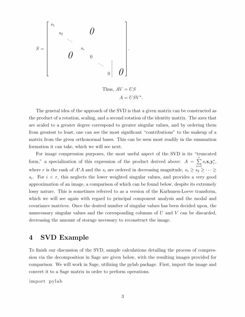
S =

s1

s2 0. . .

sr

0 0. . .

0 0

.

Thus, AV = US

A = USV ∗.

The general idea of the approach of the SVD is that a given matrix can be constructed as

the product of a rotation, scaling, and a second rotation of the identity matrix. The axes that

are scaled to a greater degree correspond to greater singular values, and by ordering them

from greatest to least, one can see the most significant “contributions” to the makeup of a

matrix from the given orthonormal bases. This can be seen most readily in the summation

formation it can take, which we will see next.

For image compression purposes, the most useful aspect of the SVD is its “truncated

form,” a specialization of this expression of the product derived above: A =r∑i=1

sixiy∗i ,

where r is the rank of A∗A and the si are ordered in decreasing magnitude, s1 ≥ s2 ≥ · · · ≥sr. For i < r, this neglects the lower weighted singular values, and provides a very good

approximation of an image, a comparison of which can be found below, despite its extremely

lossy nature. This is sometimes referred to as a version of the Karhunen-Loeve transform,

which we will see again with regard to principal component analysis and the modal and

covariance matrices. Once the desired number of singular values has been decided upon, the

unnecessary singular values and the corresponding columns of U and V can be discarded,

decreasing the amount of storage necessary to reconstruct the image.

4 SVD Example

To finish our discussion of the SVD, sample calculations detailing the process of compres-

sion via the decomposition in Sage are given below, with the resulting images provided for

comparison. We will work in Sage, utilizing the pylab package. First, import the image and

convert it to a Sage matrix in order to perform operations.

import pylab

3

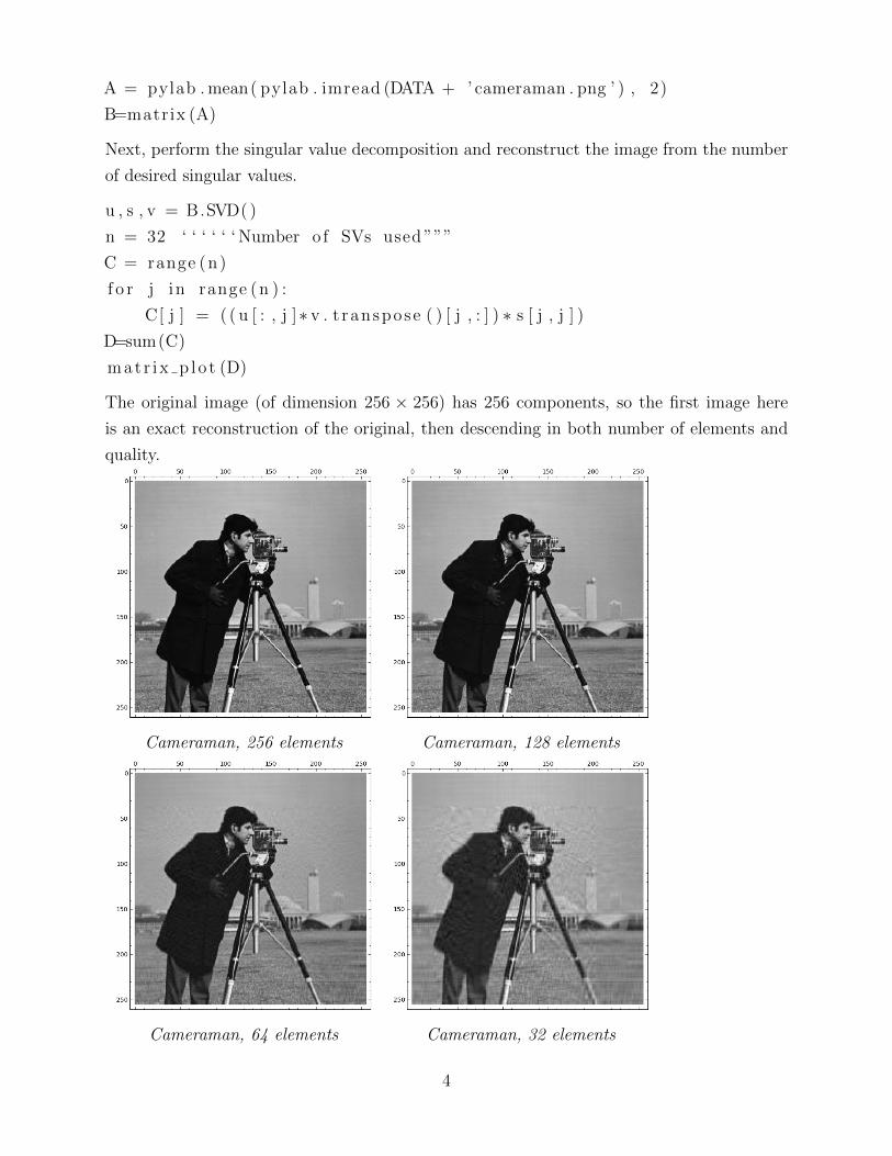
A = pylab . mean( pylab . imread (DATA + ’ cameraman . png ’ ) , 2)

B=matrix (A)

Next, perform the singular value decomposition and reconstruct the image from the number

of desired singular values.

u , s , v = B.SVD( )

n = 32 ‘ ‘ ‘ ‘ ‘ ‘ Number o f SVs used ”””

C = range (n)

f o r j in range (n ) :

C[ j ] = ( ( u [ : , j ]∗ v . t ranspose ( ) [ j , : ] ) ∗ s [ j , j ] )

D=sum(C)

mat r i x p lo t (D)

The original image (of dimension 256 × 256) has 256 components, so the first image here

is an exact reconstruction of the original, then descending in both number of elements and

quality.

Cameraman, 256 elements Cameraman, 128 elements

Cameraman, 64 elements Cameraman, 32 elements

4

Cameraman, 16 elements Cameraman, 8 elements

5 Principal Component Analysis

Principal Component Analysis can be seen as a method similar to SVD compression in the

sense that it selects the “most important” components, however, the method for doing so is

different. PCA can be seen as a statistical process for finding the best representation for a

set of data. Principal components have a wide variety of applications in many fields, such as

finding the principal moments and axes of inertia in physics. Generally, however, the process

of finding the principal components of a set of data encompasses the same basic idea, and

typically involves the solution of an eigenvalue problem.

Typically, the goal of PCA is to find an orthonormal basis for a space which orders

variables in decreasing order of their variance. In terms of information theory, the idea of a

variable’s entropy (conceptually introduced by Claude Shannon in 1948) is the basis for PCA,

wherein variables that have greater variance (or, higher entropy) carry more information,

and therefore, maximizing the variance of a particular variable will maximize the density

of information it can carry. By ordering variables in order of decreasing variance, we can

compress data via an approximation by leaving off the components that contribute the least

information, which are exactly those with low variance. In this manner, PCA is “just like”

the SVD, which places precedence on singular values of higher weights.

One method for finding the aforementioned components is through the modal matrix,

which will follow as a result from a short foray into some statistics. Since we are primarily

working with matrices m×n with discrete values, we will use the discrete case. The expected

value of a random variable, E(X) =∑xip(xi) = µ. This value can be viewed as a mean of

sorts, predicting an average outcome for a given probabilistic scenario. Variance, V (X), is

E[(X − µ)2], and can be viewed as the expected deviation from the mean, µ. The positive

square root is the familiar standard deviation. Next, the covariance or correlation of two

5

variables is Cov(X, Y ) = E[(X−µx)(Y −µy)], and if this is zero, X and Y are independent.

If X = Y then we recover our earlier definition of variance.

The covariance matrix of X is Cov(X) or∑

= E[(X − µ)T (X − µ)] where µ is the

vector of expected values µi = E(Xi). This matrix is positive semi-definite, which means its

eigenvalues will also be positive, and similar to the SVD, these are what we will order. This

is where the SVD comes into the calculations for PCA and why the K-L transform can be

seen as both SVD and PCA compression. Additionally, Cov(X) is symmetric, and therefore,

diagonalizable. The eigenvectors of the covariance matrix of X must be orthogonal, and

by scaling can be made into an orthonormal set. Setting these scaled eigenvectors as the

rows of a matrix creates the modal matrix M , whose rows are the principal axes for X, and

diagonalize the covariance matrix Cov(X).

Theorem 1. PCA Finds Principal Axes (After Hoggar [1])

Let the orthonormal eigenvectors of Cov(X), where X = X1, . . . , Xd, be R1, . . . , Rd.

Let X have components (in the sense of projection) {Yi}, where Y = Yi.

Then {Ri} is a set of principal axes for X.

Proof.

Yi = X ·Ri = XRTi

Y = XMT ,M = Rows(Ri).

Because M diagonalizes Cov(X), we can write:

Cov(Y ) = Cov(XMT ) = MCov(X)MT ,

which is a diagonal matrix of eigenvalues. Additionally, this shows that V (Yi) = λi.

If the Ri are the principal axes for X, then the Yi will be the principal components, and we

can expect them to be uncorrelated, meaning the variance of X ·Ri is maximal. This is only

true when, for an arbitrary R, R = Ri, meaning that they are the principal axes for X.

Additionally, if E(X) 6= 0, one can subtract E(X) from X, perform these calculations,

and add E(X) back. If we have d vectors X, we can transform them into k vectors Y , k < d

by discarding the Yk+1 to Yd vectors with a minimal loss of data. This is similar to SVD

compression, but instead of using the eigenvectors of a matrix itself as a basis (in combination

with singular values), we eliminate the singular values for the statistically chosen basis of

eigenvectors. Essentially, this process, which we can now formally call the K-L transform,

in the words of Hoggar, “minimizes the mean squared error for mapping d-vectors in a given

class into a space of dimension k” [1, 297].

6

Often in image compression, blocks of 8 × 8 pixels are selected and turned into vectors

of length 82 = 64. These N vectors are stacked as rows into a “class matrix” HN×64 after

subtracting the mean, then the modal matrix M is calculated, either by the method described

before or through the SVD. (If the dimension of these vectors is greater than N , performing

the same calculations with HH∗ is a quicker computation.) Once we have acquired the

principal components, we can project our data using as few or as many principal components

as we like via matrix multiplication. Similar to the discarding of unnecessary components

in SVD compression, the reduction of vector space dimension allows the image to be stored

much smaller than the original before being reconstituted.

Due to the similarity to SVD compression, we will not examine a method to perform the

Karhunen-Loeve transform in detail here, however, many authors have provided algorithms

to do so, including S. Hoggar [1] and Mark Richardson [7], including illustrations of compa-

rable quality to the SVD. One caveat, as pointed out by Hoggar, is that performing the K-L

transform utilizing SVD rather than diagonalization is numerically stabler, at the cost of a

lengthier initial computation, than other methods, such as the Discrete Cosine Transform,

which we will detail next.

6 Discrete Cosine Transform

The final method of image compression we will examine is perhaps the most popular in

practical usage as it is utilized by the JPEG file format. The discrete cosine transform is of

the family of fast Fourier transforms, and like the other transformations we have examined,

behaves linearly, allowing us to write a matrix form that is quick to compute. The one-

dimensional DCT can be written as follows, where φk is a vector with components n, written

as a variable to avoid confusion with matrix notation.

φk(n) =

√

2Ncos (2n+1)kπ

2N, for n = 1, 2, . . . , N − 1,√

1N, for n = 0.

From this definition, a set of k vectors (each of dimension n) is orthonormal and spans

the space of N -vectors. Because of this, we can easily invert the matrix of columns M =

[φ0|φ1| . . . |φN−1] by its transpose. The matrix M is applied via the matrix-vector product,

transforming input vectors which can easily be reverted through a matrix-vector product

with the inverse of M . This allows us to extend the DCT to a 2D case, where a matrix of

values can be transformed via the calculation B = MAMT .

Since the 2D case of DCT is simply a composition of the same function along each

dimension, the product is separable, and is therefore comparable to applying the 1D case

7

twice. In the case of an image, we are essentially performing the same operation on the

rows, then columns, but through matrix multiplication instead of repeated matrix-vector

products. One method for image compression utilizes a similar formulation by partitioning

an image into vectors of length 8, first by rows, then columns, and applying an 8× 8 DCT

matrix to each vector. By the end, each 8× 8 submatrix of the image has been transformed,

accomplishing the same ends as the matrix version we will explore here.

The JPEG file format utilizes the aforementioned method for the compression of images.

The primary transformation applying the DCT achieves is in moving information to the

earliest indices of a vector or matrix, leaving many of the latter entries close to zero. The

lossy part of JPEG compression happens when many of these “close to zero” entries are set

to zero, depending on the level of compression desired, a step called quantization. In the

case of the twice-applied 1D version, a particular compression setting would force the last n

indices of a vector to zero, meaning out of every 8× 8 submatrix, only (8− n)2 coefficients

out of 64 would be nonzero.

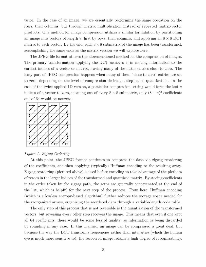
Figure 1. Zigzag Ordering

At this point, the JPEG format continues to compress the data via zigzag reordering

of the coefficients, and then applying (typically) Huffman encoding to the resulting array.

Zigzag reordering (pictured above) is used before encoding to take advantage of the plethora

of zeroes in the larger indices of the transformed and quantized matrix. By storing coefficients

in the order taken by the zigzag path, the zeros are generally concatenated at the end of

the list, which is helpful for the next step of the process. From here, Huffman encoding

(which is a lossless entropy-based algorithm) further reduces the storage space needed for

the reorganized arrays, organizing the reordered data through a variable-length code table.

The only step of this process that is not reversible is the quantization of the transformed

vectors, but reversing every other step recovers the image. This means that even if one kept

all 64 coefficients, there would be some loss of quality, as information is being discarded

by rounding in any case. In this manner, an image can be compressed a great deal, but

because the way the DCT transforms frequencies rather than intensities (which the human

eye is much more sensitive to), the recovered image retains a high degree of recognizability.

8

The most noticeable downside of JPEG compression are the “blockiness” of the 8× 8 pixel

arrays. If the compression level is sufficiently high, the blocks begin to look averaged across

the entirety of their values, losing a degree of smoothness in areas of little change and leading

to characteristically blocky looking artifacts. For natural images with a high information

density, this is not especially apparent, but for a manufactured image (such as text) that has

a high degree of contrast, the block algorithm JPEG uses is not well suited for high-quality

image recovery.

7 DCT Example

To finish, we will apply the DCT as an example, with some code provided. As before, we

utilize pylab to import the image.

import pylab

A = pylab . mean( pylab . imread (DATA + ‘ k l e i n r e s i z e d . png ’ ) , 2)

B = matrix (A)

Next, create the 8× 8 DCT matrix, M .

M=matrix (RR, 8 )

from sage . symbol ic . cons tant s import p i

PI = pi

f o r i in range ( 1 , 8 ) :

f o r j in range ( 8 ) :

M[ i , j ] = ( s q r t (1/4)∗ cos ( (2∗ j +1)∗ i ∗PI / (2∗8 ) ) )

f o r j in range ( 8 ) :

M[ 0 , j ] = 1/ s q r t (8 )

Now we will partition our image into 8×8 blocks. Since our image has dimension 200×160,

there will be 20 blocks along the horizontal and 25 along the vertical for a total of 500 blocks.

It will then be multiplied with the DCT matrix, the product of which is shown here.

y = range (500)

f o r j in range ( 2 0 ) :

f o r i in range ( 2 5 ) :

y [ j +20∗ i ]=B[ ( i ∗ 8 ) : ( i ∗8+8) ,( j ∗ 8 ) : ( j ∗8+8)]

x = range (500)

f o r i in range ( 5 0 0 ) :

x [ i ]=M∗y [ i ]∗M. transpose ( )

DCT = block matr ix (25 ,20 , x )

9

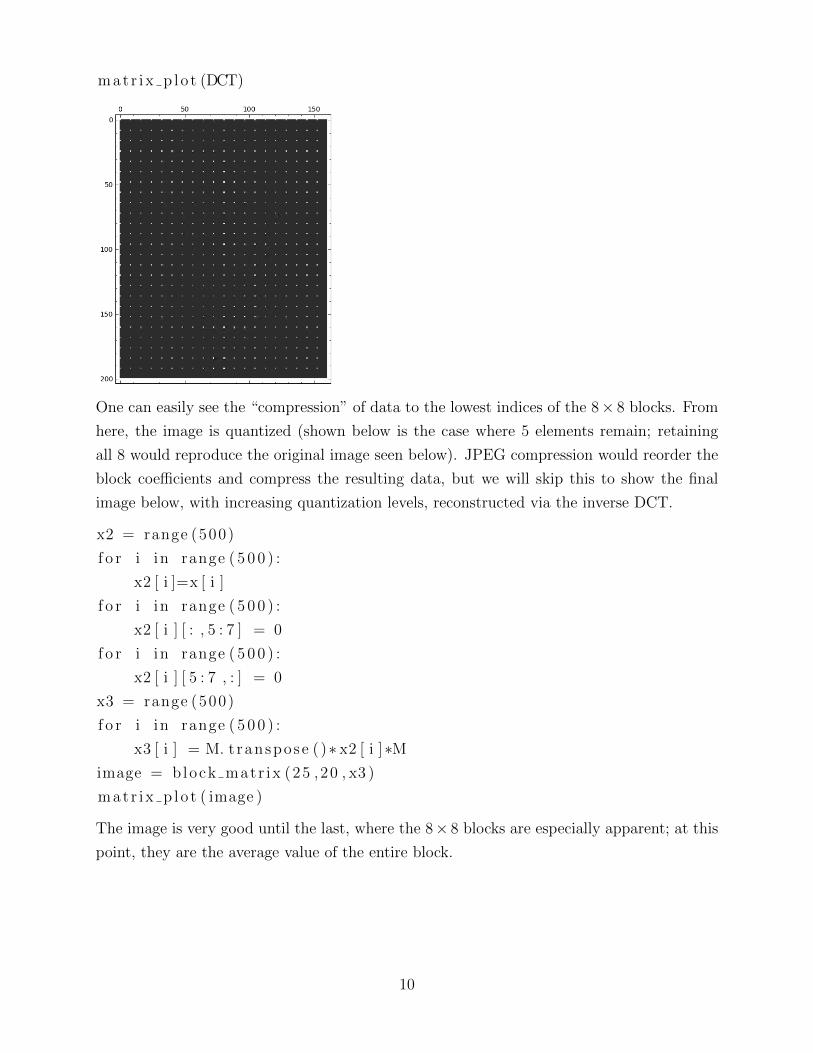
matr ix p lo t (DCT)

One can easily see the “compression” of data to the lowest indices of the 8× 8 blocks. From

here, the image is quantized (shown below is the case where 5 elements remain; retaining

all 8 would reproduce the original image seen below). JPEG compression would reorder the

block coefficients and compress the resulting data, but we will skip this to show the final

image below, with increasing quantization levels, reconstructed via the inverse DCT.

x2 = range (500)

f o r i in range ( 5 0 0 ) :

x2 [ i ]=x [ i ]

f o r i in range ( 5 0 0 ) :

x2 [ i ] [ : , 5 : 7 ] = 0

f o r i in range ( 5 0 0 ) :

x2 [ i ] [ 5 : 7 , : ] = 0

x3 = range (500)

f o r i in range ( 5 0 0 ) :

x3 [ i ] = M. t ranspose ( )∗ x2 [ i ]∗Mimage = block matr ix (25 ,20 , x3 )

mat r i x p lo t ( image )

The image is very good until the last, where the 8× 8 blocks are especially apparent; at this

point, they are the average value of the entire block.

10

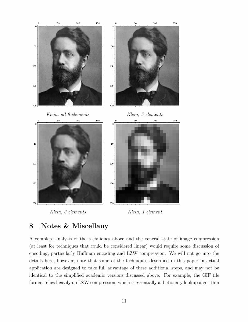
Klein, all 8 elements Klein, 5 elements

Klein, 3 elements Klein, 1 element

8 Notes & Miscellany

A complete analysis of the techniques above and the general state of image compression

(at least for techniques that could be considered linear) would require some discussion of

encoding, particularly Huffman encoding and LZW compression. We will not go into the

details here, however, note that some of the techniques described in this paper in actual

application are designed to take full advantage of these additional steps, and may not be

identical to the simplified academic versions discussed above. For example, the GIF file

format relies heavily on LZW compression, which is essentially a dictionary lookup algorithm

11

that works surprisingly well for natural images. The images used for the example calculations

in this paper are in the PNG format, a spiritual successor to the GIF file format.

9 Conclusion

Through our discussion of two similarly styled compression methods (SVD and PCA) that

make use of matrices’ natural characteristics (eigenvalues), as well as an industry standard

transform (DCT for JPEG), we have seen a variety of approaches to the multifaceted subject

of compression, at least for natural images. As is apparent from the nature of the calculations

being performed, linear algebra is particularly well-suited to the task, and the methods

developed take full advantage of the speed and accuracy afforded by linear operations. A

logical next step in a fuller understanding of compression could focus on wavelets and fractals,

as well as entropy compression and information theory. However, for a basic understanding of

the principles and methods of image compression, the three methods discussed here represent

a useful and straightforward introduction to the art.

10 References

[1] Hoggar, S. G. Mathematics of digital images: creation, compression, restoration, recog-

nition. Cambridge: Cambridge University Press, 2006.

[2] N. Ahmed, T. Natarajan and K.R. Rao. “Discrete Cosine Transform.” IEEE Trans.

Computers, 90-93, Jan. 1974.

[3] Lay, David. Linear Algebra and its Applications. New York: Addison-Wesley, 2000.

[4] Trefethen, Lloyd N., and David Bau. Numerical linear algebra. Philadelphia: Society

for Industrial and Applied Mathematics, 1999.

Additional web resources:

[5] http://introcs.cs.princeton.edu/java/95linear/

[6] http://www.uwlax.edu/faculty/will/svd/

[7] http://people.maths.ox.ac.uk/richardsonm/SignalProcPCA.pdf

11 License

This work is licensed under the Creative Commons Attribution-ShareAlike 4.0 International

License. To view a copy of this license, visit http://creativecommons.org/licenses/

by-sa/4.0/ or send a letter to Creative Commons, 444 Castro Street, Suite 900, Mountain

View, California, 94041, USA.

12