math 3340: fixed income mathematics or the theory of

Math 3340: Fixed Income Mathematics orThe Theory of Interest Fall 2020

Instructor: Dr Giles Auchmuty

* * *

email: auchmuty at uh.eduURL: https://www.math.uh.edu/∼giles/

Office: PGH 696 Tel: 713-743-3475.

A prerequisites and course description are available on myweb site. A syllabus with lots of official information is nowavailable on the Access UH website

This course will not follow any current text very closely.The theory of interest has been studied since biblical times

in many different parts of the world. It is essential for all trade andbusiness as merchants ( people who buy and sell goods ) are inthe situation where they pay for the goods at one time and thenreceive payment from someone else later.

Bankers, pawnbrokers, mortgage companies, factors andmany different types of lenders make their living by arrangingtransactions that include interest charges. Interest is the cost ofborrowing, or lending, money. The mathematical theory ofinterest is the study of the formulae involved.

Will and Ariel Durant in ”The Lessons of History” said

... those who manage money manage all.

For a long time this was a topic where there were few laws.The Truth in Lending Act was only passed in 1968 and providedsome legal definitions that will be used here - including APR

This course is about the formulae used for managing money- assuming that everyone is honest and pays. In practice therealways is a possibility of default or someone not paying what theowe. This means that you must add probability theory to thecalculations. So one of the first required actuarial exams is onprobability theory + interest theory.

The essential results that you should learn from this courseinclude

I the formulae for loans and mortgages.

I How to evaluate the present value of a string of payments -such as pensions and annuities.

I How to price treasury bills and government bonds. Theevaluation of current yield, duration, convexity.

I How leverage affects returns on bonds and otherinvestments.

I Formulae for the evaluation of portfolios.

Probability theory is not a prerequisite for this course andwill not be used, or needed, here. But to apply the ideas to realworld situations, you do need to include probabilistic ideas.

Unfortunately there is no text that describes the simplemathematics behind each of these topics. Hence no required textfor the course. When I first taught this course I used the bookThe theory of Interest, 3rd ed, Stephen G. Kellison, McGraw Hill

More recently An Introduction to the Mathematics ofMoney, Lovelock, Mendel and Wright, Springer, has been usedas a text.

There are hundreds of thousands (sometimes millions) ofpostings on the Web about each of these topics. Wikipedia haslots of articles on various aspects. In general I’ll try to use actuarialnotation (as in Kellison’s text) but some of that notation is rarelyused now and everybody now uses spreadsheets for most of theircalculations.

Neither of the above texts uses spreadsheets, or personalcomputers. They are outdated for teaching - but the theory hasn’tchanged. It is also hard to use more than 1 source for this materialas everyone seems to have a different notation.

You will need to use spreadsheets for doing the homework. Ifyou don’t already have one that you know how to use; I suggestApache OpenOffice which is free and can be downloaded inversions for most operating systems and languages.

A lot of the theory here uses the same mathematical ideas asis used in biology for describing growth and population dynamics.Plants and critters breed rather than earn interest - but theformulae for their population and size are similar and have similarproofs.

Growth Factors and Interest rates

Throughout this course we will be using the symbol Am foran amount at time tm and Am is usually measured in units of USdollars, (sometimes thousands or millions of US dollars.)

At increasing times {t0 < t1 < t2 < . . . < tm < . . .} supposethe value of an account is {0 < A0,A1,A2, . . . ,Am, . . .}. Then theratio

fm :=Am

Am−1is called the m-th growth factor

of the account and measures the change between times tm−1, tm.Equivalently the value of the account satisfies the equation

Am = fm Am−1 for m = 1, 2, 3, . . . .

The interest rate in the m-th time interval is rm wherefm := 1 + rm. Note rm := fm − 1 usually is a small number - andhopefully positive.

Example 1. A person puts $1,000 in a bank account that paysinterest of 1% a month for 12 months. How much does she haveafter each month and at the end of a year?

At each time tm, an interest payment of $Am−1/100 for theperiod (tm−1, tm) is added to the account so

Am = 1.01 Am−1 with A0 = 1000.

That is she receives $10 after 1 month, $10.10 (or 1% of $1010 )for interest in the 2nd month etc.

The growth factor for this account is f = 1.01 and theinterest rate is r = .01 = 1% and do not depend on m.

Note that both growth factors and interest rates are simplenumbers. A percentage x% is just the number x/100. For example5% is the number .05 = 5/100.

If an account has a uniform interest rate f = 1 + r for Mtime periods, then the value of an account at time tm when itstarted with initial amount A0 has

A1 = f A0, A2 = f 2 A0, A3 = f 3 A0, A4 = f 4 A0, . . .

That isAm = f m A0 = (1 + r)m A0 (1)

This is the Compound Interest Formula.

In finance we usually just determine amounts at discretetimes, such as daily, weekly, monthly, every quarter, half-year oryear.

Then the growth factors and interest rates are per day, perweek, per month, ... You may think that an interest rate of 1% permonth, would be the same as 3% per quarter, 6% per half-year or12% per year - but they are NOT.

As an exercise evaluate the value after 1 year of the accountthat had an initial amount $1,000 and had each of thesecompounding rates.

A calculator yields that(1.01)12 = 1.126825, (1.03)4 = 1.12551, (1.06)2 = 1.1236so after 1 year she would have respectively

$1126.82, $1125.51, $1, 123.60 and $1120.00

In finance we usually just determine amounts at discretetimes, such as daily, weekly, monthly, every quarter, half-year oryear.

Then the growth factors and interest rates are per day, perweek, per month, ... You may think that an interest rate of 1% permonth, would be the same as 3% per quarter, 6% per half-year or12% per year - but they are NOT.

As an exercise evaluate the value after 1 year of the accountthat had an initial amount $1,000 and had each of thesecompounding rates. A calculator yields that(1.01)12 = 1.126825, (1.03)4 = 1.12551, (1.06)2 = 1.1236so after 1 year she would have respectively

$1126.82, $1125.51, $1, 123.60 and $1120.00

The difference here could be up to $7 or so depending onhow often the interest is compounded. The more often a givennominal annual rate of interest ra is compounded, the larger theinterest amount.

When you earn interest at an annual rate of ra compoundedk times a year, then the amount is given by

Am =(

1 +rak

)Am−1 so Am =

(1 +

rak

)mA0

is the value after m time periods (or m payments).

This is why banks and brokerages usually charge dailyinterest rates on loans, mortgages usually have monthly interestpayments while bonds usually pay interest only every 6 months.

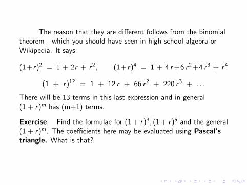
The reason that they are different follows from the binomialtheorem - which you should have seen in high school algebra orWikipedia. It says

(1+r)2 = 1 + 2r + r2, (1+r)4 = 1 + 4 r +6 r2+4 r3 + r4

(1 + r)12 = 1 + 12 r + 66 r2 + 220 r3 + . . .

There will be 13 terms in this last expression and in general(1 + r)m has (m+1) terms.

Exercise Find the formulae for (1 + r)3, (1 + r)5 and the general(1 + r)m. The coefficients here may be evaluated using Pascal’striangle. What is that?

Since the actual growth depends on how often interest iscompounded, the federal law now requires that whenever aninterest rate is given, and in additon to what ever nominalformula is described, the annual percentage rate APR mustbe given. The APR of an account is r := f − 1 where f is thegrowth rate on the account over 1 year or

f := A1year/A0

This enables a person to compare the cost of different interestformulae. Two sets of compounding formulae are said to beequivalent if they yield the same APR and annual growth rate.

Inthe preceding example the APRs are, respectively,

0.1268 = 12.68%, 0.1255 = 12.55%, 12.36% and 12%

depending on whether they are compounded monthly, quarterly,half-yeraly or annually.

Since the actual growth depends on how often interest iscompounded, the federal law now requires that whenever aninterest rate is given, and in additon to what ever nominalformula is described, the annual percentage rate APR mustbe given. The APR of an account is r := f − 1 where f is thegrowth rate on the account over 1 year or

f := A1year/A0

This enables a person to compare the cost of different interestformulae. Two sets of compounding formulae are said to beequivalent if they yield the same APR and annual growth rate. Inthe preceding example the APRs are, respectively,

0.1268 = 12.68%, 0.1255 = 12.55%, 12.36% and 12%

depending on whether they are compounded monthly, quarterly,half-yeraly or annually.

Exercise. What is the APR of a nominal interest rate of 0.12 =12% compounded daily? Find the various interest rates of anyloans or credit cards that you, or your family, maintain. See whatdifferent rates they describe and see if you can verify theirequivalence.

The Compound Interest Formula is the basic formula fordoing any calculation in interest theory.

Am = f m A0 = (1 + r)m A0 (2)

Note that it involves 4 variables A0,Am, r and m. It is anequation, so whenever three of these numbers are given, there areways to find the possible value, or values, of the fourth.

Problem 1. The simplest calculation is given A0,m, r , to findAm. This problem was solved earlier.

Problem 2. A variation on Problem 1 is to ask how much youneed to invest in this account if you want to have an amount$1,000 after 1 year? That is, given m = 12,A12 = 1000, r = 0.01to find A0.

In this case the equation becomes

1000 = 1.126825 A0 since 1.0112 = 1.126825.

so A0 = $887.45

The general solution is A0 = (1 + r)−m Am

This is the expression for the initial amount as a function ofthe final amount, the nominal rate and the number of payments.

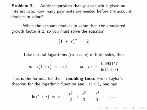
Problem 3. Another question that you can ask is given aninterest rate, how many payments are needed before the accountdoubles in value?

When the account doubles in value then the associatedgrowth factor is 2, so you must solve the equation

(1 + r)m = 2

Take natural logarithms (to base e) of both sides, then

m ln (1 + r) = ln 2 or m =0.693147

ln (1 + r)

This is the formula for the doubling time. From Taylor’stheorem for the logathmic function and |r | < 1, one has

ln (1 + r) = r − r2

2+

r3

3− r4

4+ . . . .

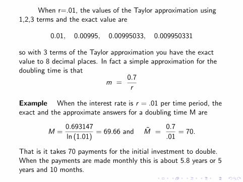
When r=.01, the values of the Taylor approximation using1,2,3 terms and the exact value are

0.01, 0.00995, 0.00995033, 0.009950331

so with 3 terms of the Taylor approximation you have the exactvalue to 8 decimal places. In fact a simple approximation for thedoubling time is that

m =0.7

r

Example When the interest rate is r = .01 per time period, theexact and the approximate answers for a doubling time M are

M =0.693147

ln (1.01)= 69.66 and M =

0.7

.01= 70.

That is it takes 70 payments for the initial investment to double.When the payments are made monthly this is about 5.8 years or 5years and 10 months.

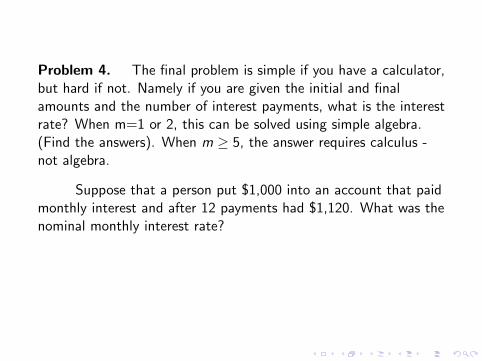
Problem 4. The final problem is simple if you have a calculator,but hard if not. Namely if you are given the initial and finalamounts and the number of interest payments, what is the interestrate? When m=1 or 2, this can be solved using simple algebra.(Find the answers). When m ≥ 5, the answer requires calculus -not algebra.

Suppose that a person put $1,000 into an account that paidmonthly interest and after 12 payments had $1,120. What was thenominal monthly interest rate?

In this case m=12, and(1 + r)12 = 1.12. Then r = 1.12(1/12) − 1 = .0094888 orabout 0.95% per month.

Problem 4. The final problem is simple if you have a calculator,but hard if not. Namely if you are given the initial and finalamounts and the number of interest payments, what is the interestrate? When m=1 or 2, this can be solved using simple algebra.(Find the answers). When m ≥ 5, the answer requires calculus -not algebra.

Suppose that a person put $1,000 into an account that paidmonthly interest and after 12 payments had $1,120. What was thenominal monthly interest rate? In this case m=12, and(1 + r)12 = 1.12. Then r = 1.12(1/12) − 1 = .0094888 orabout 0.95% per month.

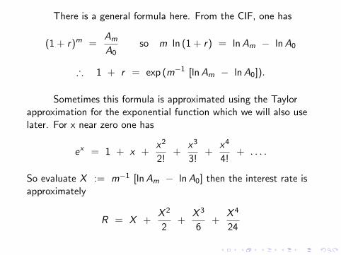
There is a general formula here. From the CIF, one has

(1 + r)m =Am

A0so m ln (1 + r) = ln Am − ln A0

∴ 1 + r = exp (m−1 [ln Am − ln A0]).

Sometimes this formula is approximated using the Taylorapproximation for the exponential function which we will also uselater. For x near zero one has

ex = 1 + x +x2

2!+

x3

3!+

x4

4!+ . . . .

So evaluate X := m−1 [ln Am − ln A0] then the interest rate isapproximately

R = X +X 2

2+

X 3

6+

X 4

24

Account Equations

Most accounts involve the payment of interest each periodtogether with either deposits or withdrawals for an account duringthe period. For such accounts, the balance in each time period is

Am = fm Am−1 + cm for m = 1, 2, 3, . . . .

Here fm = 1 + rm is the m-th growth factor and cm is thecontribution in the m-th time interval. When cm < 0, then there isa withdrawal from the account.

In the following please find, and write up for your ownbenefit, any algebra and calculus term or theorem that isused. They will be needed repeatedly

For mathematical analysis we will just treat the case wherthe interest rate and the contributions are constant. This holds ifit is a savings account based on payroll deduction or a retirementaccount where there are equal contributions every time period.

Then the equation becomes

Am = (1 + r) Am−1 + c for m ≥ 1

By repeated substitiution one sees that the solution of theisequation is

Am = (1 + r)m A0 + c [1 + f + f 2 + . . .+ f m−1]

(Verify this for m=1,2,3 please.)

This may be simplified by using the formula for geometricalsums - which you should have seen in high school. it says that

1 + f + f 2 + . . .+ f m−1 =f m − 1

f − 1when f 6= 1

Question Find this sum when f=1 and then obtain the formulafor Am when r=0. Does your answer make sense?

For r 6= 0, the solution of a uniform account equation is

Am = (1 + r)m A0 +c

r[(1 + r)m − 1]] for m ≥ 1. (3)

For any value of r, the expression (1 + r)m is apolynomial of degree m in r, that has the form

(1+r)m = 1 + m r +m(m − 1)

2r2 +

m(m − 1)(m − 2)

6r3 + . . .

from the binomial theorem. The . . . indicates powers of r4, r5

and higher order powers when m is larger.

The linear approximation of a solution is

Am = (1 + r)m A0 + c m

[1 +

(m − 1)

2r

](4)

The quadratic approximation of a solution includes the r2

term and is

Am = (1 + r)m A0 + c m

[1 +

(m − 1)

2r +

(m − 1)

6(m − 2) r2

](5)

Example Suppose a person has an account that pays 1% permonth. She makes and initial deposit of $1,000 and then adds $50each month. What is the balance in the account after one year?

Comments: Any time you have a problem like this I suggest thatyou start by guessing an approximate answer. In this case, if noextra contributions were made, you know from the compoundinterest formula, that the $1,000 will become more than $1,126.Then she added $600 in contributions. So the answer is probablylarger than $1,730 - thanks to the interest on her contributions.This is just a guess - and you may want to guess another number.

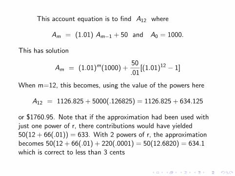
This account equation is to find A12 where

Am = (1.01) Am−1 + 50 and A0 = 1000.

This has solution

Am = (1.01)m(1000) +50

.01[(1.01)12 − 1]

When m=12, this becomes, using the value of the powers here

A12 = 1126.825 + 5000(.126825) = 1126.825 + 634.125

or $1760.95.

Note that if the approximation had been used withjust one power of r, there contributions would have yielded50(12 + 66(.01)) = 633. With 2 powers of r, the approximationbecomes 50(12 + 66(.01) + 220(.0001) = 50(12.6820) = 634.1which is correct to less than 3 cents

This account equation is to find A12 where

Am = (1.01) Am−1 + 50 and A0 = 1000.

This has solution

Am = (1.01)m(1000) +50

.01[(1.01)12 − 1]

When m=12, this becomes, using the value of the powers here

A12 = 1126.825 + 5000(.126825) = 1126.825 + 634.125

or $1760.95. Note that if the approximation had been used withjust one power of r, there contributions would have yielded50(12 + 66(.01)) = 633. With 2 powers of r, the approximationbecomes 50(12 + 66(.01) + 220(.0001) = 50(12.6820) = 634.1which is correct to less than 3 cents

Note that our guess and all the approximations are belowthe exact answer. Also notice that these formulae require the useof the binomial theorem from algebra and Taylor’s theorem forapproximating functions in calculus 1. These theorems will be usedrepeatedly in this class - and in financial calculations - so makesure that you know them.

The solution of an account equation gives Am as a functionof the 4 quantities, A0, c ,m, r . Thus it is an equation in 5variables. If you know 4 of these quantities then you chould be ableto find the fifth. I will give some homework problems of this type.

Another example is a simple college savings plan or othergift plan. Suppose your parents, grandparents or favorite auntdecides to save on a regular savings plan so they can give you a biggift on your 21st birthday, for your college expenses or whatever.

They invest in a program, or possibly buy an insurancepolicy, that will pay you $10,000 at a certain time in the futureprovided you pay a certain amount $A0 now and contribute $c permonth. These savings accumulate at a certain interest rate, say0.5% a month payable monthly.

Usually the questions are either(i) How much do they need to pay iniitialy if they can afford tocontribute $100 a month and it will be 60 months in the future? or(ii) If they can put $5,000 now into such an account whatmonthly payments do they have to make?

Answer (i) The problem is to find $A0 given that

m = 60, A60 = 10, 000, c = 100 and r = 0.005.

The solution of the account equation (3) becomes

10000 = (1.005)60 (A0 + 20000) − 20000

as c/r = 20000. Thus

A0 + 20000 = 30000/1.34885 = 22241.17

or A0 = 2241.17 is the exact answer for this problem. It maybe rounded to $2250 initially plus $6,000 in total contributions +interest payments of about 6% per year for 5 years.

The linear approximation here leads to the equation

10000 = (1.005)60 A0 + 6000 (1 + 29.5(0.005))

10000 = (1.005)60 A0 + 6000 (1 + 29.5(0.005))

1.34885A0 = 10000 − 6885 = 3115

This yieds that A0 = 2309.37 - which is a larger amount thanthe exact answer as we have undercounted the interest earned.

Similarly you can determine the value of A0 from thequadratic approximation and this will be less than 2309 and morethan 2242.

Examples such as these show that even the simplest interesttheory problems are completely changed by the advent ofcomputers and programs that guarantee the correct solutions usinggood mathematics for solving equations.

Moreover if you decide to change the interest rate or thenumber of years in these solutions, and you have a spread sheet - itis quite straightforward. The second homework will ask you todevelop a spreadsheet that does these caculations for a problemlike this. The important thing is to have the spread sheet - thenyou can plug in whatever are the relevant numbers and see whatthe answer is.

Answer (ii) The problem is to find $C given that

m = 60, A0 = 5000, A60 = 10000, and r = 0.005.

The solution of the account equation (3) becomes

10000 = (1.005)60 5000 + 200C (0.34885)

as 1/r = 200. Thus

69.77C = 3255.75 or C = 46.66

To check this note that 60 payments of $47 is $2820 andtogether with the initial $5000 they contribute $7820 towards the10K value at the end. This earns much more interest as it starts at5K instead of less than 2.3K in the previous calculation.

Similarly for this problem one can ask about finding r or mwhen the other 4 variables are known. It is high school math toshow how the equations can be ”rearranged” so that there is theunknown on one side of the equation and numbers on the otherside, so you just have to do a direct calculation.

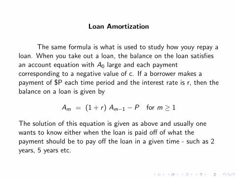
Loan Amortization

The same formula is what is used to study how youy repay aloan. When you take out a loan, the balance on the loan satisfiesan account equation with A0 large and each paymentcorresponding to a negative value of c. If a borrower makes apayment of $P each time period and the interest rate is r, then thebalance on a loan is given by

Am = (1 + r) Am−1 − P for m ≥ 1

The solution of this equation is given as above and usually onewants to know either when the loan is paid off of what thepayment should be to pay off the loan in a given time - such as 2years, 5 years etc.

The loan repayment formula says that if you have a loan of$L at an interest rate of r per time period, and make regularpayments of $P, then after m time period the outstanding balanceon the loan is, from the solution of the account equation

Am = (1 + r)m L − P

r[(1 + r)m − 1]] for m ≥ 1. (6)

Usually the questions about this loan is what should P be topay the loan off in M payments, or what is the value of M suchthat this loan is paid off with regular payments of $P.

Note that this formula doesn’t involve the actual timeperiod. The answers are the same whether we take the time periodto be days, weeks, months or years!

If the loan is paid off in M time periods, then AM = 0 so onehas

P

r

[(1 + r)M − 1]

]= (1 + r)M L (7)

That is

P = p(r ,M)L with p(r ,M) =r (1 + r)M

[(1 + r)M − 1](8)

This says that the payment is linear in the loan amount L -which makes sense but it is a complicated function of r and M.This function is an increasing function of r for fixed M and adecreasing function of M for fixed r.

This is proved by evaluating the partial derivative ofp(r ,M) with respect to r,M respectively. Suggest that you trythis, we’ll look at this later.

The next few slides are to remind you of some calculusresults that will be used a lot. Suggest that you review the reasonswhy they hold and perhaps try to see which apply to variousformulae described so far.

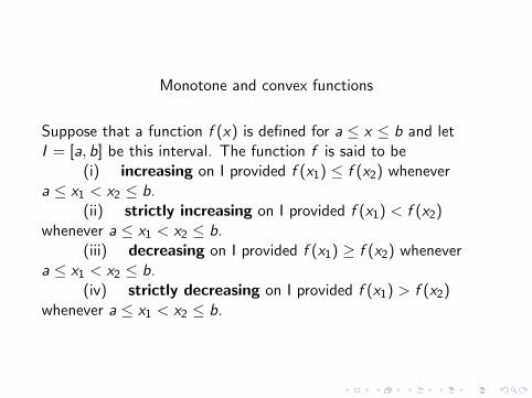
Monotone and convex functions

Suppose that a function f (x) is defined for a ≤ x ≤ b and letI = [a, b] be this interval. The function f is said to be

(i) increasing on I provided f (x1) ≤ f (x2) whenevera ≤ x1 < x2 ≤ b.

(ii) strictly increasing on I provided f (x1) < f (x2)whenever a ≤ x1 < x2 ≤ b.

(iii) decreasing on I provided f (x1) ≥ f (x2) whenevera ≤ x1 < x2 ≤ b.

(iv) strictly decreasing on I provided f (x1) > f (x2)whenever a ≤ x1 < x2 ≤ b.

In calculus I you should have learnt that when f isdifferentiable on the open interval (a,b), then

(a) the function f is increasing (decreasing) on I wheneverf ′(x) ≥ (≤)0 for x ∈ (a, b).

(b) the function f is strictly increasing (strictly decreasing)on I whenever f ′(x) > (<)0 for x ∈ (a, b).

The function is (strictly) monotone on I if it is either(strictly) increasing or decreasing on I.

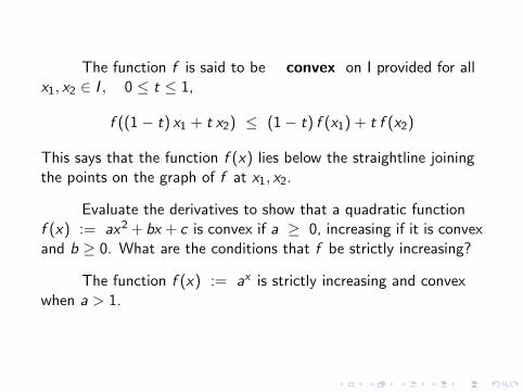
The function f is said to be convex on I provided for allx1, x2 ∈ I , 0 ≤ t ≤ 1,

f ((1− t) x1 + t x2) ≤ (1− t) f (x1) + t f (x2)

This says that the function f (x) lies below the straightline joiningthe points on the graph of f at x1, x2.

Evaluate the derivatives to show that a quadratic functionf (x) := ax2 + bx + c is convex if a ≥ 0, increasing if it is convexand b ≥ 0. What are the conditions that f be strictly increasing?

The function f (x) := ax is strictly increasing and convexwhen a > 1.

In general when f is continuously differentiable and thederivative f ′(x) is increasing on (a, b), then f is convex.

When f is twice continuously differentiable and f ”(x) ≥ 0on a < x < b, then f is convex on I.

The function f is concave on I when each ≤ is replacedby ≥ above. Alternatively f is concave when −f is convex.

The function l(x) := loga x is strictly increasing andconcave when a > 1, x > 0. For many of the formulae in financeand the theory, it is important to prove inequalities for the valuesof functions and their derivatives - as you will see. You just needto know how to calculate the derivatives.

Example. Show that the doubling time for a simple savingsaccount with interest rate r is strictly decreasing and convex.Proof. The doubling time is given by the functiong(r) := ln 2/ ln (1 + r) with r > 0. Evaluate the derivative

g ′(r) =dg

dr(r) = . . .

Observe that this derivative is always negative and you can verifythat g ′(r) is an increasing function of r. Since the functionln (1 + r) is strictly increasing, g is strictly decreasing.

If you are an ace at calculus, you might get the right answerfor the second derivative of g(r). Suggest that you use aspreadsheet or a program to graph this function - and its firstderivative to show that the function is convex.

Very often with compound interest the interest rate changeseach time period, and is given by

Am = (1 + rm) Am−1 = fm Am−1 for m ≥ 1.

Then the first few values are

A1 = f1A0, A2 = f2 f1 A0, A3 = f3 f2 f1 A0, ...

In generalAm = fm fm−1 . . . , f2 f1 A0

Often we replace all these different growth factors by asingle average growth factor to do calculations. This growth factorwill be the solution of

f m = fm fm−1 . . . , f2 f1

This number is called the geometric mean of the positive valuesf1, . . . , fm and is given by

fg := [f1 f2 . . . , fm−1 fm ]1/m

It is easy to prove that for 2 positive numbers x1, x2

√x1 x2 ≤ (x1 + x2)/2

or the geometric mean of two numbers is less that the usual meanvalue.

This geometric mean is an equivalent growth factor forwhich we can use the formulae for constant (or uniform) growth.When each fm = 1 + rm, the equivalent uniform interest rate isrg where

fg = 1 + rg

The solutions of the uniform interest payments case with theequivalent uniform rate and the variable interest rate cases usuallyare very close. So when there are variable interest rates, peopleoften just evaluate the equivalent uiform rate and use the formulaewe’ve obtained earlier.

How good this is, requires a lot more calculus which is whymathematicians are useful for some calculations in finance.

The arithmetic-geometric mean inequality (AGM) isthe fact that for any M positive numbers a1, . . . , aM , this stillholds. That is, the geoemetric mean of M positive numbers is lessthan the arithmetic mean unless they all are equal.

ag := [a1 a2 . . . , aM−1 aM ]1/M ≤ 1

M[a1 + a2 . . .+ aM−1 + aM ]

The arithmetic mean will usually be denoted

a :=1

M[a1 + a2 . . .+ aM−1 + aM ]

so the AGM inequality is that ag ≤ a. Sometimes one alsouse the obvious fact that

ag ≥ a with a = min {a1, . . . , aM}.

when you want to check a calculation.

Example. Suppose that a dealer lends you $10,000 to help payfor a car. You have good credit, so he charges a nominal interestrate 0.06 = 6% per year payable monthly for 2 years. How muchwill each payment be? What is the total payment and how muchinterest will you pay?

First note that the paperwork should tell you this loan hasAPR 0.0617 = 6.17%. Why this rate? Use the formula withM = 24, r = 0.005 then (1.005)24 = 1.12716 so

p(r ,M) =0.0056358

0.12716= 0.0443205

This each payment is P = 443.21Your total payment is 24P = 10636.93 and the total

interest payment is $636.93.

Earlier we used the fact that

(1 + r)M = 1 + Mr[1 + br + cr2 + . . .

]with b = (M − 1)/2, c = (M − 1)(M − 2)/6 and said thatusually in calculations we only need these terms in mostevaluations. The formula for the M uniform payments P on a loanof L dollars with interest rate r per time period becomes, whenbr , cr2 can be neglected

P = p0(r ,M) L with p0(r ,M) = r +1

M

In the previous example this is 0.0466.67 for payments of 466.67per month.

The linear approximation, which neglects cr2 is

P = p1(r ,M) L with p1(r ,M) = r +1

M(1 + br)

The quadratic approximation is

P = p2(r ,M) L with p2(r ,M) = r +1

M(1 + br + cr2)

Since b, c > 0 when M ≥ 3 these factors decrease as more termsare included.

You can do the calculations for the auto loan above. Foreach of these approximations, you may check to see if they areincreasing functions of r and decreasing fuctions of M

In view of these formulae, you can also look at questionssuch as, if you can only afford to make payments of about $360 amonth on the car, then how many payments will you have to make?

You can write an algorithm to solve this exactly. Howevercould also. just take the simplest approximation and see that atthis interest rate you want

(.005 + 1/M) 10000 ≤ 360

This yields M = 62.5 so it seems that a 5-year loan with 60payments should work. Suggest that you evaluate the exact cost ofsuch a loan.

Similarly, if the dealer says that they will lend you the fundswith repayments of $450 per month for 24 months, then you knowthat they are charging you a slightly higher APR than 0.0617 =6.17% .

If you want to find the interest rate that is being chargedthen you would have to solve the equation

r (1 + r)M

(1 + r)M − 1=

P

L= : ρ

Here ρ is the proportion of the regular payment to the original loanamount. Note that you must have MP > L when the interest ratesare positive, so ρ > 1/M and the interest rate is a positive solutionof the equation

(1 + r)M(r − ρ) + ρ = 0

Let x := 1 + r , then this equation becomes

f (x) := xM+1 − (1 + ρ) xM + ρ = 0 (9)

This is the interest rate equation for a loan. To find the interestrate, solve this equation for a solution x near 1 and then theinterest rate will be r := x − 1.

There are algebraic formulae for the solutions of theseequations when M=1,2 and 3 but not in general for M ≥ 4.However, x = 1 is a solution with f ′(1) < 0 when ρ > 1/M.Thus f (x) is below 0 for x > 1 and close to 1. It is easy to showthat there is no solution of this equation larger than 1 + ρ. Somemore calculus shows that there is a unique solution with

xM :=M(1 + ρ)

M + 1< x < 1 + ρ.

as f (x) is strictly increasing for x > xM .

Computing Zeros of Equations.

The simplest algorithm for solving the equation f (x) = 0,when one knows values x1, x2 with f (x1) < 0 < f (x2) is thebisection method. It is guaranteed to yield a solution when f iscontinuous on I := [x1, x2] and it will be the unique solution iff ′(x) > 0 on I. This is the intermediate value theorem fromcalculus I.

Usually one just seeks to find a value x with |f (x)| < εwhereε > 0 is a small number. If one want f (x) to be zero to 3 decimalplaces, take ε = 0.0005. Sometimes we just want the answer tosome accuracy δ.

The Bisection Algorithm.

The bisection algorithm is given I1; = [x1, x2], f and δ, ε as above,Step 1. For j ≥ 1, Ij := [x1, x2], evaluate |Ij | = x2 − x1,ξ = (x1 + x2)/2, and f (ξ).Step 2. If |Ij | < δ, or |f (ξ)| < ε take ξ to be the solution andstop.Step 3. Otherwise when f (ξ) ≥ ε, replace x2 by ξ so thatIj+1 = [x1, ξ]. If f (ξ) ≤ −ε, take Ij+1 = [ξ, x2] and go to step 1.

With this algorithm, one sees that |Ij+1| = |Ij |/2 so theinterval containing a zero decreases in size by a factor of 2 at eachstep. It guarantees that in a finite number of steps either |Ij | < δ,or |f (ξ)| < ε, so we have found an approximate zero of thefunction f (x).

It is quite easy to implement a spreadsheet program to usethe bisection method for solving an equations such as the interestrate equation. Note you only have to evaluate the function f (x) -no derivatives or any other functions are required. Please write youown spread sheet program to solve equations of the form(1 + x)m = 2 with m=2 -10. These provide formulae for doublingtimes for a simple compound interest problem. The first step is tomake good choices for x1, x2. Choose sime good guesses.

if you have that when x1 < x2 one has f (x1) > 0 > f (x2)so there still is a zero in the interval, then use g(x) := −f (x) andthe function g will have the properties required for the bisectionalgorithm to work.

Present Value of a future Payment

People value a payment of $P more highly today than thepromise of a payment of the. same amount at some time in thefuture. Also it is worth more if it will be1 week in the futurecompared to 1 month in the future, 1 year in the future or 5 yearsin the future. That is the longer you have to wait the lower thepresent value PV.

Suppose it costs $ PV today to buy a contract for anamount of $ A in T years time, then the discount rate d(T)of this contract is

d(T ) :=PV

Aor PV = d(T ) A

Here PV is the present value of the payment $ A in T years timeand d(T) is usually between 0 and 1.

The annual discount rate of this contract is

da := d(T )1/T

Discount rates measure the time value of money and may berelated to interest rates. An annual discount rate corresponds toan APR of ra where

da =1

1 + raor ra =

1− da

da

Discount rates may also are quoted in terms of weeks, months orother time periods.

See Wikipedia, or other internet sites, for descriptons ofthese ideas with many different notations and conventions. Theimportant aspect is that in these contracts, the amount to bereturned at time T is the fixed amount $A and the “price” is theimmediate cost of this promise - that is, the present value.

Example. Four grandparents want to make a gift of $10,000cash to a grandchild on her 21st birthday in 3 years time. Someare in ill-health and are not sure that they will be around, or havethe money then, so they pay $9,700 for a certificate of deposit inher name that will be worth $10,000 when it matures 3 years later.

Here the 3-year discount rate is d(3) = 0.97 so the annualdiscount rate is 0.98990 which corresponds to earning an APR of0.0111 =1.11%. Suggest that you check this, and all similarevaluations so you know what formulae are used.

Example. A company has just made a big sale and realizes thatit will have to pay the governent at least a million dollars in taxesin 6 months time. The cost of a 6-month T-bill is $990 so it buys1000 such bills to ensure that it can pay this amount. What is theannual discount rate, and APR, of these bills?

The discount rate of these bills is d(1/2) = 0.99, theannual discount rate is da = 0.992 = 0.9801 and ra is 2.03%..

These contracts are also called a single premium annuity andmay be arranged with banks, various brokers and some governmentagencies as well as with individuals and companies. The federalgovernment sells T-bills in multiples of a thousand dollars and fordifferent time lengths via auctions.

If you search Wikipedia, or the internet for annuities,certificates of deposit, zero-coupon bonds or similar keywords youwill find many different businesses that will be pleased to take yourmoney now in exchange for some promise to pay you back in thefuture.

Your primary concern should be whether they will actuallydo so - or whether they will “default”. Government issuedcontracts (T-bills, bonds, notes) are regarded as “riskless” or“safe” - since the government also ”prints the money” or ”controlsthe currency”. However even governments occasionally default ontheir promises; particularly after wars.

Annuities

An annuity is a series of payments at specified times in thefuture. Examples include

the payout of lottery prizes as amounts of $P each year for20 or 30 years,

Divorce, injury or other legal payments of $P a month for aspecified number of months.

Many people buy retirement annuities that pay $P eachmonth, or quarter or ... for a fixed number of years starting at age70 or some other age.

Many annuities are “ life annuities” that make payments forthe rest of a person’s life (such as social security payments andmany retirement programs). The mathematics of those depend onthe probability that a person will lives to various ages - so theyshould use life tables and need probability theory for thecalculations. This is a big business for insurance companies.

If you search for annuity on the internet there are lots ofprovider advertising and also of people who will advise you (for afee) on possible annuities to buy.

There also are many annuity calculators which essentiallyjust are small programs that do the calculations that I’ll describehere. A good example is the Present Value of Annuity Calculatorat financialmentor .com who say they provide “Financial freedomfor Smart Prople”.

The following slides will describe the models and formulaebehind the simpler examples. Often people want to add extraconditions and requirements to a ”boilerplate” policy.

Suppose an annuity consists of M payments of $ A startingnow and paid N times a year. An insurance company prices theannuity at a uniform discount rate of da per year. Then the m-thpayment is due at time tm := m/N years from now and haspresent value

PVm = (da)m/N A = dm A

where d = (da)1/N is the discount rate per payment.

Then the present value of the annuity is the sum of eachindividual annuity so if it starts after 1/N years, then

PV = PV1 + PV2 + . . .+ PVM

PV =[d + d2 + . . .+ dM

]A =

d (1 − dM)

1− dA

using the formula for geometric sums.

More generally if the payment starts after K time periodsfrom now, then

PV =M−1∑m=0

dK+m A

and this sum is

PV =dK (1 − dM)

1− dA

Here K could be any positive number or even zero and measuresthe “waiting time” to the first payment. These are the AnnuityEquations that say how much an annuity should cost at a givendiscount rate.

The annuity equation may be written

PV = vMK (d)A with vMK (d) :=dK (1 − dM)

1− d

Here vKM(d) is called the annuity factor. It is a decreasingfunction of K, M and an increasing function of d for 0 < d < 1.When M is very large, the distant (m large) payments have verysmall present value. If M = ∞ these are called perpetuities,that have an infinte payout but finite present value!

The present value of a perpetuity of $A per payment,starting K time periods from now at a discount rate d is

PVP :=dK

1− dA

These are promises to pay “forever” and are not legal inmost states and countries but are often used for pricing annuitieswith M very very large such as for 100-year leases for property.

Note that a lease with uniform fixed payments at fixed times(weekly, monthly, quarterly, etc) is a simple annuity. Usually toevaluate the present value of a lease, you need to treat depositsseparately.

Example. What is the cost of an annuity that pays $1000 everyfour weeks for 52 weeks starting in a year’s time if it is bought atan annual discount rate of 0.96? The cost uses the precedingformulae evaluated with 4 week periods. The discount rate eachfour weeks is d = 0.961/13 = 0.996865. Then

PV = 9600.04

.003135. = 960(12.75917) = 12248.80.

That is, an insurance company offering this annuity should quote aprice of $12,248.80 to the buyer. They will then pay out a total of$13,000 to the recipient of the annuity

Often this is the way “trust fund babies” are paid or patientsin a nursing home. The trust fund buys such an annuity, then theinsurance company makes this arranged payout to the designatedbeneficiary.

Continuous Interest rates

We have seen that a nominal interest rate of r per yearcharged daily leads to a daily interest rate of (r/365) so the APRis given by

1 + ra =(

1 +r

365

)365since the daily growth factor is fd = (1 + r

365).

Example A nominal interest rate of r = 0.1825 compoundeddaily has an APR of ra = .20016 or 20.016%.

One of the definitions of the exponential function is that

ex := limm→∞

(1 + x/m)m

Thus a nominal annual interest rate of r compounded continuously(that is every second of every day) will yield an annual percentagerate of ra := er or a growth factor of r(T ) = erT over T years.

Example. The nominal interest rate of 18.25% per yearcompounded continuously has an APR of ra = .20021 which isonly very slightly higher than daily compounding.

We say that an account earns an annual continuousinterest rate rc provided its growth factor after time T is

f (T ) := ercT or A(T ) = A(0) ercT

Thus an account that earns interest with an APR of ra peryear has continuous interest rate rc := ln (1 + ra) as theannual growth rates are f = 1 + ra = erc

This says that an annual rate of ra paid once a year isequivalent to an interest rate of rc every second during the year (tomany decimal places) as they have the same 1-year growth factors.

Example. What is the continuous interest rate corresponding toan APR of 0.1 = 10%?

Ans: rc = ln 1.1 = 0.095310

When interest is compounded more often than weekly, mostpeople use continuous compounding since it simplifies many of themathematical formulae.

The continuous rate always obeys rc < ra as ln (1 + x) < xfor x > 0. From the Taylor series for the exponential function onesees that

ra = rc +1

2rc

2 +1

6rc

3 + ...

so rc will be close to (and below) the solution of

x2 + 2 x − 2 ra = 0.

This is the equation you get from just using 2 terms in the Taylorseries. A better approximation is the solution that uses 3 termsand is a cubic equation for an approximation of rc .

Just as there is an APR associated with any discrete interestrate so also there is a continuous interest rate associated with anydiscrete interest rate. Suppose r2 is an interest rate per 1/2 year,r4 is an interest rate per quarter, r12 is an interest rate per ordinarymonth and r52 is a weekly interest rate. Then the continuousinterest rate rc associated with these rates satisfies

erc = (1 + r2)2 = (1 + r4)4 = (1 + r12)12 = (1 + r52)52

Each of these is the 1-year growth factor at the indicated rate.

Exercise What is the similar formulae for the 4-week interestrate r13 and the daily interest rate r365? Complete the followingformulae for r13, r52, r365.

rc = 2 ln (1 + r2) = 4 ln (1 + r4) = 12 ln (1 + r12) = ...

When a continuous interest rate r is known, then the growthfactor of an investment of $A for time T is

f (T ) := erT so A(T ) = A erT

The present value of a payment of $A to be made at time T in thefuture is

PV = d(T ) A with d(T ) = e−rT =1

f (T )

US Treasury Bills or T-bills

See Wikipedia entry for United States Treasury security.

These are issued by the US government who promise to payyou $1,000 per bill in 4, 8, 13, 26 or 52 weeks time from the dateof purchase. An M week bond has a term or time to maturity ofM weeks.

Buyers pays $10 P per bill with P < 100 being determinedby an auction. Since these are government bonds they areconsidered to be “riskless” and have the lowest interest rates ofany bonds available in the US for this time period. So T-bill ratesare used for comparison purposes to all other interest rates.

Suppose that an M week T -bills is sold for a price of $10P,then we say that the M-week treasury (continuous) interest rate isrk per year where

P = 100e−(k rk ) and k = 52/M.

Thus the 52-week T-bill rate is the annual continuousinterest rate associated with this purchase. The 26-week T-bill rateis the semi-annual continuous interest rate per year The 13-weekT-bill rate is the quarterly continuous interest rate and the 4-weekT-bill rate is the (lunar) monthly interest rate per year.

A plot of interest rate against time to maturity, or term, iscalled a yield curve.

Example 1. If a 12-month T-bill costs $980, then we say its priceis P = $98.00. The 52-week T-bill continuous rate is ra where

era = 100/98 = 1.0204082. Thus

ra = ln 1.0204082 = 0.02020271

This is a continuous rate of 2.02% per year.

Example 2. A 6-month T-bill costs $991.00 so its price is said tobe P= $99.10. The 26-week T-bill continuous rate is r2 where

er2 = 100/99.1 = 1.0090817 Thus

r2 = 2 ln 1.0090817 = 0.0180815

This is a continuous rate of 1.808% per year.

Zero Coupon Bonds

T- bills are special examples of what are called zero couponbonds (ZCB). These are bonds that do not make any interestpayments but which will pay a given amount $A at time T fromnow. A is called the face value of this bond and T is the term orthe time to maturity. The present value of a bond with face value$A, at the continuous interest rate r is

PV = A e−rT

We say the price of such a bond is P = 100 e−rT < 100 andassume that r > 0, T > 0. So the price is the cost of such a bondwith face value $100 at maturity.

Example. What is the price of a ZCB that pays a continuousinterest rate of 3% and has 3 years to maturity?Answer. P = 100 e−0.09 = $91.3931. Thus each $1,000 bondwill cost $913.93.

Problem A 4-year ZCB is bought for $900. What is thecontinuous interest rate for this bond?

This time want to find r, when 900 = 1000 e−4r . .Thus e4r = 1.111111111 so 4r = .1053605 andr = 0.02634 or the interest rate is 2.634%.

In this problem, the solution for r is often called the internalrate of return (IRR) or the yield on this bond. This IRR is thendenoted by y (for yield).

Usually one has that the interest rate on shorter term bondfrom a company or government to be less than that of a longerterm bond so one expects the yield curve to be an increasingfunction of the time-to maturity (or term). If there is a range of“terms” where the yield decreases as the term increases then onehas an “ inverted” yield curve and a trader could make a profitusing riskless “arbitrage” . This could happens when there is likelyto be a big change between the maturity dates such as adeclaration of war or a difficult election.

Banks usually pay interest rates on savings and CDs that arebelow the annual interest rates on T-bills - as they often purchaseT-bills with the funds. On Wikipedia, and in older texts theydescribe the “discount yield” of a T-bill. This is a number that isvery, very close to this continuous yield per year.

math 3340: fixed income mathematics or the theory of

Documents