math 249 notes - university of waterloo 249 notes ian goulden april 4, 2008 1 lecture of january 9...
TRANSCRIPT
MATH 249 NOTES
Ian Goulden
April 4, 2008
1 Lecture of January 9
The first six weeks of the course will be concerned with Enumerative Combinatorics, alsoreferred to as Enumeration, Combinatorial Analysis or, simply, Counting. This subject con-cerns the basic question of determining the number of elements in a finite set of mathematicalobjects.
Let [n] = {1, . . ., n}, for each n ≥ 1, and [0] denote the empty set. A permutation of [n] isan ordered list of the elements of [n], each element appearing once in the list. For example,there are 6 permutations of [3], namely 123, 132, 213, 231, 312, 321. When n = 0, wesay that there is a single permutation, which happens to be an empty list. We begin byanswering a basic counting question: how many permutations are there of [n] ? The answer,given below, can be compactly expressed using factorial notation. For each nonnegativeinteger n, define n!, by 0! = 1, and
n! =
n∏
i=1
i, for n = 1, 2, . . ..
We say “n factorial” for n!.
Example 1.1 The number of permutations of [n] is n!, for n = 0, 1, . . ..
Proof. For n = 0, the result is true by the conventions above. For n ≥ 0, each permutationof [n] is of the form a1a2. . .an, where a1, a2, . . ., an are distinct elements of [n]. There aretherefore n choices for a1. No matter what choice is made for a1, there are then n−1 choicesfor a2, since a2 cannot equal a1. In fact, iteratively choosing aj+1, since a1, . . ., aj are alldifferent, then aj+1 must be chosen from the remaining n−j elements, for j = 0, 1, . . ., n−1,and so the number of choices for the permutation a1a2. . .an is
∏n−1j=0 (n− j) = n!, giving the
result.
A k-subset of [n] is a subset of [n] of size k, for k = 0, 1, . . ., n (when k = 0, the emptyset is such a subset, for any n ≥ 0). For example, there are 6 2-subsets of [4], namely {1, 2},{1, 3}, {1, 4}, {2, 3}, {2, 4}, {3, 4}. We now consider another basic counting question: howmany k-subsets are there of [n] ? The answer, given below, can be compactly expressed
1
using binomial coefficient notation. For nonnegative integers n and k = 0, 1, . . ., n, define(n
k
)by (
n
k
)=
n!
k!(n− k)!
We say “n choose k” for(
n
k
). Note that we immediately have the symmetry result
(n
k
)=
(n
n− k
).
Example 1.2 The number of k-subsets of [n] is(
n
k
), for n = 0, 1, . . ., and k = 0, 1, . . ., n.
Proof. Let x be the number of k-subsets of [n]. We determine x indirectly, by counting thepermutations of [n]. For any permutation a1. . .an and any fixed k = 0, . . ., n, the elementsin a1, . . ., ak form a k-subset of [n], call it α. Then the elements in ak+1, . . ., an form thecomplement, α, of α with respect to [n]. For example, with n = 7 and k = 3, for thepermutation 5247316 we have α = {2, 4, 5} and α = {1, 3, 6, 7}. For each fixed α, there arek! choices of a1. . .ak, since it is a permutation of α, and (n− k)! choices of ak+1. . .an, sinceit is a permutation of α. Since there are x choices of α, we conclude that the number ofpermutations of [n] is equal to
k! (n− k)! x
But this is also equal to n!, and we have proved that x =(
n
k
).
The binomial coefficients provide the answer to many counting questions. One method ofproof is to find a 1:1 correspondence between the objects being counted and an appropriateset of subsets. We give two examples of this.
Example 1.3 Prove that the number of k-subsets of [n] with no consecutive pairs of elementsis(
n−k+1k
).
Proof. Let A be the set of k-subsets of [n] with no consecutive pairs of elements, and letB be the set of k-subsets of [n − k + 1]. For example, with n = 7 and k = 3, we have
A = {135, 136, 137, 146, 147, 157, 246, 247, 257, 357},
B = {123, 124, 125, 134, 135, 145, 234, 235, 245, 345},where we have written each of the subsets as an increasing list of its elements, with nobrace brackets. We know that |B| =
(n−k+1
k
), so we establish the result by giving a 1:1
correspondence between A and B, since then we know that |A| = |B|. We claim thatf : B → A defined by
f(α) = 0 1. . .k − 1 + α,
is a 1:1 correspondence, where the addition above means that 0 is added to the first elementof α, 1 is added to the second element, and so on, until k − 1 is added to the last (andbiggest) element of α. We leave the proof that f is 1 : 1 as an exercise.
In the second example, we consider lattice paths, which are paths on the integer latticein two dimensions, with steps either North by one unit (“N”) or East by one unit (“E”).
2
Example 1.4 Prove that the number of lattice paths from (0, 0) to (m,n) is equal to(
m+n
n
),
or(
m+n
m
).
Proof. Each lattice path from (0, 0) to (m,n) contains exactly m+n steps, with n up andm right. Therefore we can represent them uniquely as an ordered list s1. . .sm+n, in whichsi = N for n choices of i, and si = E for the remaining m choices of i. Let α denote the setof all i for which si = N . Then α is an n-subset of [n + m], and this is a 1:1 correspondence.The result follows, since there are
(m+n
n
)choices of α.
For example, there are(52
)paths from (0, 0) to (3, 2), given by NNEEE,NENEE,
NEENE,NEEEN,ENNEE,ENENE, ENEEN,EENNE,EENEN,EEENN .
When m = n = 0, we say that there is exactly one path, with no steps, which agrees inthis case with the value of the binomial coefficient in Example 1.4.
From Example 1.4 with m = n, we know that there are(2n
n
)lattice paths from (0, 0)
to (n, n). We are now going to consider the number cn, n = 0, 1, . . . of these paths thatnever go below the line y = x. These paths are called Catalan paths. For example, wehave c3 = 5, since the Catalan paths with n = 3 are given by NNNEEE,NNENEE,NNEENE,NENNEE,NENENE.
We are going to prove that
cn =1
n + 1
(2n
n
), n = 0, 1, . . ..
These numbers are called Catalan numbers.
2 Lecture of January 11
Let Pn, n ≥ 0, be the set of lattice paths from (0, 0) to (n, n), represented as a string ofN ’s and E’s (which are the steps of the path) Let P ′
n, n ≥ 0, be the set of lattice pathsfrom (0,−1) to (n, n), starting with N . Then each path in P ′
n has n+ 1 N ’s and n E’s, and|Pn| = |P ′
n|.The length of a path π = π1. . .πm is |π| = m, equal to the number of steps in π. We let
∆0(π) = −1, and ∆i(π) equal the number of N ’s in the first i steps of π minus the numberof E’s in the first i steps of π, minus 1, for i = 1, . . ., m. For π ∈ P ′
n, we have ∆2n+1(π) = 0.The following result is easy to verify.
Proposition 2.1 Suppose π = αβ ∈ P ′n, where |α| = k, |β| = j, where k, j ≥ 0 (and of
course |π| = k + j = 2n + 1). Let ω = βα (called a cyclic rearrangement of π), where∆k(π) = m. Then ∆i(ω) = ∆i+k(π)−m− 1, for i = 0, . . ., j, and ∆i(ω) = ∆i−j(π)−m, fori = j + 1, . . ., 2n+ 1.
Now let Cn be the set of paths in Pn which never go below the line y = x. Considerπ ∈ P ′
n, and let M be the minimum value of ∆i(π), for i = 0, . . ., 2n + 1. Let L be themaximum value of i such that ∆i(π) = M . Then clearly M ≤ −1, and 0 ≤ L ≤ 2n,since ∆0(π) = −1, and ∆2n+1(π) = 0. Let π = αβ, where |α| = L, and ω = βα. ThenProposition 2.1 proves immediately that ∆0(ω) = −1, and ∆i(ω) ≥ 0, for i = 1, . . ., 2n+ 1.
3
But this means that ω = Nψ, where ψ ∈ Cn. For π ∈ P ′n, this proves that ω is the unique
path among the n + 1 cyclic rearrangements of π starting with N , with ω = Nψ, ψ ∈ Cn.But there are n+ 1 distinct cyclic rearrangements of any path in P ′
n, so we conclude that
|Cn| =1
n + 1
(2n
n
), n = 0, 1, . . ..
3 Lecture of January 14
The proof that we’ll consider carefully here involves a recurrence for the sequence {cn}n≥0,and the generating series
C(x) =∑
n≥0
cnxn
for this sequence, where cn = |Cn|, n ≥ 0.
Example 3.1 The sequence {cn}n≥0 satisfies the recurrence
cn =
n−1∑
k=0
ck cn−k−1, n = 1, 2, . . ., (1)
with initial condition c0 = 1.
Proof. For n ≥ 1, let π be a Catalan path from (0, 0) to (n, n). Then the first step in πmust be up. Now, π must end on the line y = x, and consider the first time after the initialup-step that π returns to the line y = x, which must be with a right-step. Then we canwrite π = Nπ1Eπ2, where π1 and π2 are Catalan paths with a total of 2n − 2 steps, takentogether. Thus if π1 has 2k steps, then there are ck choices for π1, and cn−k−1 choices for π2.The result follows by summing over k = 0, . . ., n− 1.
Note that the recurrence in Example 3.1, together with the initial condition, uniquelygenerates the sequence {cn}n≥0. For example, we have c0 = 1 from the initial condition, thensuccessively compute from the recurrence:
c1 = c20 = 1,
c2 = c0 c1 + c1 c0 = 2,
c3 = c0 c2 + c21 + c2 c0 = 5.
We now solve the recurrence (1). The first step is to show that the generating series C(x)satisfies a simple equation.
Example 3.2 The generating series C(x) satisfies the quadratic equation
xC(x)2 − C(x) + 1 = 0.
4
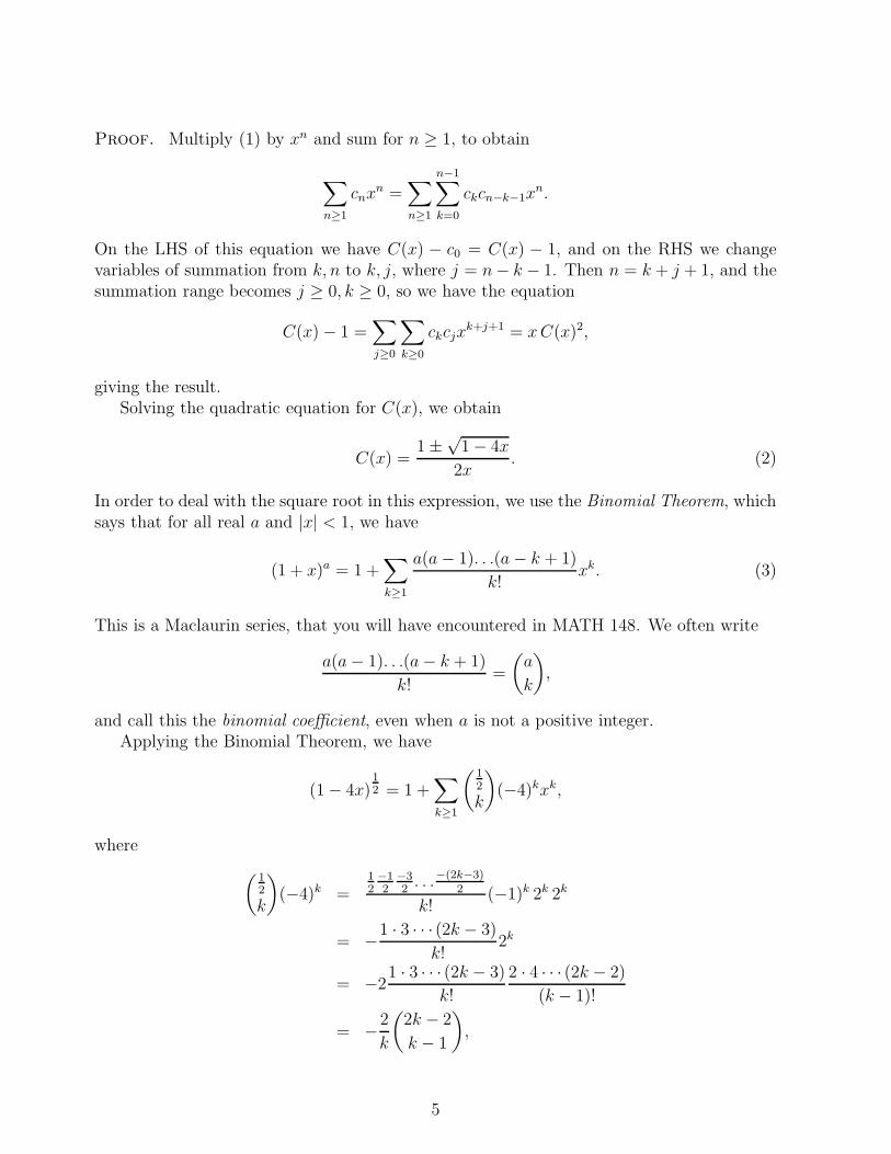
Proof. Multiply (1) by xn and sum for n ≥ 1, to obtain
∑
n≥1
cnxn =
∑
n≥1
n−1∑
k=0
ckcn−k−1xn.
On the LHS of this equation we have C(x) − c0 = C(x) − 1, and on the RHS we changevariables of summation from k, n to k, j, where j = n− k − 1. Then n = k + j + 1, and thesummation range becomes j ≥ 0, k ≥ 0, so we have the equation
C(x) − 1 =∑
j≥0
∑
k≥0
ckcjxk+j+1 = xC(x)2,
giving the result.Solving the quadratic equation for C(x), we obtain
C(x) =1 ±
√1 − 4x
2x. (2)
In order to deal with the square root in this expression, we use the Binomial Theorem, whichsays that for all real a and |x| < 1, we have
(1 + x)a = 1 +∑
k≥1
a(a− 1). . .(a− k + 1)
k!xk. (3)
This is a Maclaurin series, that you will have encountered in MATH 148. We often write
a(a− 1). . .(a− k + 1)
k!=
(a
k
),
and call this the binomial coefficient, even when a is not a positive integer.Applying the Binomial Theorem, we have
(1 − 4x)12 = 1 +
∑
k≥1
( 12
k
)(−4)kxk,
where
(12
k
)(−4)k =
12−12
−32. . .−(2k−3)
2
k!(−1)k 2k 2k
= −1 · 3 · · · (2k − 3)
k!2k
= −21 · 3 · · · (2k − 3)
k!
2 · 4 · · · (2k − 2)
(k − 1)!
= −2
k
(2k − 2
k − 1
),
5
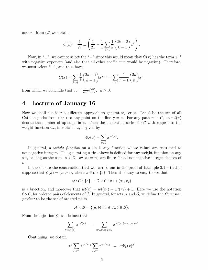
and so, from (2) we obtain
C(x) =1
2x±(
1
2x− 1
x
∑
k≥1
1
k
(2k − 2
k − 1
)xk
).
Now, in “±”, we cannot select the “+” since this would mean that C(x) has the term x−1
with negative exponent (and also that all other coefficients would be negative). Therefore,we must select “−”, and thus have
C(x) =∑
k≥1
1
k
(2k − 2
k − 1
)xk−1 =
∑
n≥0
1
n+ 1
(2n
n
)xn,
from which we conclude that cn = 1n+1
(2n
n
), n ≥ 0.
4 Lecture of January 16
Now we shall consider a different approach to generating series. Let C be the set of allCatalan paths from (0, 0) to any point on the line y = x. For any path π in C, let wt(π)denote the number of up-steps in π. Then the generating series for C with respect to theweight function wt, in variable x, is given by
ΦC(x) =∑
π∈C
xwt(π).
In general, a weight function on a set is any function whose values are restricted tononnegative integers. The generating series above is defined for any weight function on anyset, as long as the sets {π ∈ C : wt(π) = n} are finite for all nonnegative integer choices ofn.
Let ψ denote the construction that we carried out in the proof of Example 3.1 – that issuppose that ψ(π) = (π1, π2), where π ∈ C \ {ε}. Then it is easy to easy to see that
ψ : C \ {ε} → C × C : π 7→ (π1, π2)
is a bijection, and moreover that wt(π) = wt(π1) + wt(π2) + 1. Here we use the notationC×C, for ordered pairs of elements of C. In general, for sets A and B, we define the Cartesianproduct to be the set of ordered pairs
A×B = {(a, b) : a ∈ A, b ∈ B}.
From the bijection ψ, we deduce that∑
π∈C\{ε}
xwt(π) =∑
(π1,π2)∈C×C
xwt(π1)+wt(π2)+1
Continuing, we obtain
x1∑
π1∈C
xwt(π1)∑
π2∈C
xwt(π2) = xΦC(x)2.
6
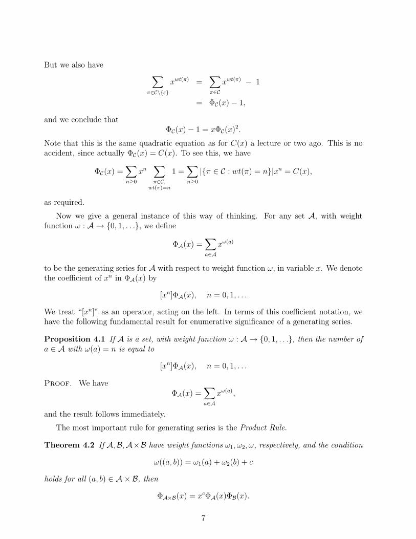
But we also have∑
π∈C\{ε}
xwt(π) =∑
π∈C
xwt(π) − 1
= ΦC(x) − 1,
and we conclude thatΦC(x) − 1 = xΦC(x)
2.
Note that this is the same quadratic equation as for C(x) a lecture or two ago. This is noaccident, since actually ΦC(x) = C(x). To see this, we have
ΦC(x) =∑
n≥0
xn∑
π∈C,wt(π)=n
1 =∑
n≥0
|{π ∈ C : wt(π) = n}|xn = C(x),
as required.
Now we give a general instance of this way of thinking. For any set A, with weightfunction ω : A → {0, 1, . . .}, we define
ΦA(x) =∑
a∈A
xω(a)
to be the generating series for A with respect to weight function ω, in variable x. We denotethe coefficient of xn in ΦA(x) by
[xn]ΦA(x), n = 0, 1, . . .
We treat “[xn]” as an operator, acting on the left. In terms of this coefficient notation, wehave the following fundamental result for enumerative significance of a generating series.
Proposition 4.1 If A is a set, with weight function ω : A → {0, 1, . . .}, then the number ofa ∈ A with ω(a) = n is equal to
[xn]ΦA(x), n = 0, 1, . . .
Proof. We haveΦA(x) =
∑
a∈A
xω(a),
and the result follows immediately.
The most important rule for generating series is the Product Rule.
Theorem 4.2 If A,B,A×B have weight functions ω1, ω2, ω, respectively, and the condition
ω((a, b)) = ω1(a) + ω2(b) + c
holds for all (a, b) ∈ A× B, then
ΦA×B(x) = xcΦA(x)ΦB(x).
7

Proof. We have
ΦA×B(x) =∑
(a,b)∈A×B
xω((a,b))
=∑
a∈A
∑
b∈B
xω1(a)+ω2(b)+c
= xc∑
a∈A
xω1(a)∑
b∈B
xω2(b),
and the result follows.
For sets A1, . . .,Ak, and fixed positive integer k, the product rule extends easily to setsof k-tuples
A1 × . . .×Ak = {(a1, . . ., ak) : a1 ∈ A1, . . ., ak ∈ Ak}.
Theorem 4.3 (Product Rule for k-tuples) If A1, . . .,Ak,A1× . . .×Ak have weight functionsω1, . . ., ωk, ω, respectively, and the condition
ω((a1, . . ., ak)) = ω1(a1) + . . .+ ωk(ak) + c
holds for all (a1, . . ., ak) ∈ A1 × . . .×Ak, then
ΦA1×...×Ak(x) = xcΦA1
(x). . .ΦAk(x).
Example 4.4 Find the number of solutions to t1 + . . . + tk = n, where t1, . . ., tk are non-negative integers.
SOLUTION. Let S = A1 × . . . × Ak, where Ai = {0, 1, 2, . . .}, for i = 1, . . ., k. For(a1, . . ., ak) ∈ S, let ω((a1, . . ., ak)) = a1 + . . . + ak. Then the answer to this problem isprecisely the number of elements in S with weight function value equal to n, which is equalto
[xn]ΦS(x).
Now note that ω((a1, . . ., ak)) = τ(a1) + . . .+ τ(ak), where τ is the identity function, so theproduct rule for k-tuples gives
ΦS(x) = ΦA1(x). . .ΦAk
(x) = Φ{0,1,2,...}(x)k,
whereΦ{0,1,2,...}(x) =
∑
i∈{0,1,2,...}
xi = 1 + x1 + x2 + . . .,
since the weight function is the identity. Thus the answer is given by
[xn](1 + x1 + x2 + . . .)k = [xn]((1 − x)−1
)k= [xn](1 − x)−k,
by summing the geometric series.
8
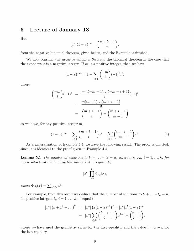
5 Lecture of January 18
But
[xn](1 − x)−k =
(n+ k − 1
n
),
from the negative binomial theorem, given below, and the Example is finished.
We now consider the negative binomial theorem, the binomial theorem in the case thatthe exponent a is a negative integer. If m is a positive integer, then we have
(1 − x)−m = 1 +∑
i≥1
(−mi
)(−1)ixi,
where(−m
i
)(−1)i =
−m(−m − 1). . .(−m− i+ 1)
i!(−1)i
=m(m+ 1). . .(m+ i− 1)
i!
=
(m+ i− 1
i
)=
(m+ i− 1
m− 1
),
so we have, for any positive integer m,
(1 − x)−m =∑
i≥0
(m+ i− 1
i
)xi =
∑
i≥0
(m+ i− 1
m− 1
)xi. (4)
As a generalization of Example 4.4, we have the following result. The proof is omitted,since it is identical to the proof given in Example 4.4.
Lemma 5.1 The number of solutions to t1 + . . . + tk = n, where ti ∈ Ai, i = 1, . . ., k, forgiven subsets of the nonnegative integers Ai, is given by
[xn]
k∏
i=1
ΦAi(x),
where ΦAi(x) =
∑j∈Ai
xj.
For example, from this result we deduce that the number of solutions to t1 + . . .+ tk = n,for positive integers ti, i = 1, . . ., k, is equal to
[xn](x+ x2 + . . .
)k= [xn]
(x(1 − x)−1
)k= [xn]xk(1 − x)−k
= [xn]∑
i≥0
(k + i− 1
k − 1
)xk+i =
(n− 1
k − 1
),
where we have used the geometric series for the first equality, and the value i = n − k forthe last equality.
9
Of course, this problem can be solved without generating series, using various moreelementary methods, such as set bijections. For example, we can note that if t1+ . . .+tk = n,where t1, . . ., tk are positive integers, then {t1, t1 + t2, . . ., t1 + . . .+ tk−1} is a (k − 1)-subsetof {1, . . ., n − 1}. Moreover, if {α1, . . ., αk−1}, with 1 ≤ α1 < . . . < αk−1 ≤ n − 1, is a(k− 1)-subset of {1, . . ., n− 1}, then (α1, α2 −α1, . . ., αk−1 −αk−2, n− αk−1) is a solution tothe equation t1 + . . .+ tk = n. It is straightforward then to check that we have a bijection,which proves that the number of solutions in this case is
(n−1k−1
).
However, when we modify such problems even in a simple way, they can become verycomplicated to deal with by elementary means, yet the generating series methodology handlesthem straightforwardly, using perhaps more binomial expansions. Consider the followingexample.
Example 5.2 Find the number of solutions to t1 + . . .+ tk = n, where t1, . . ., tk are positiveintegers not equal to 3.
SOLUTION. From Lemma 5.1, with Ai = {1, 2, 4, 5, . . .}, for i = 1, . . ., k, the answer is givenby
[xn]
(x
1 − x− x3
)k
= [xn]
k∑
i=0
(k
i
)(x
1 − x
)k−i
(−x3)i
= [xn]k∑
i=0
(k
i
)(−1)ixk+2i(1 − x)−(k−i)
Continuing with our solution, from the negative binomial theorem we obtain
[xn]
k∑
i=0
∑
j≥0
(k
i
)(−1)i
(k − i+ j − 1
j
)xk+2i+j =
∑
i
∑
j
(k
i
)(−1)i
(k − i+ j − 1
j
),
where the double sum on the righthandside is over all j ≥ 0, 0 ≤ i ≤ k, subject to therestriction that k + 2i + j = n. Thus we can replace j by n − k − 2i, and write this as asingle sum
∑
i
(k
i
)(−1)i
(n− 3i− 1
k − i− 1
),
where this sum ranges from 0 to min{k, ⌊n−k2⌋}. We have used the floor function ⌊x⌋, for
the real number x, whose value is the greatest integer not greater than x. The inequalityi ≤ ⌊n−k
2⌋ arises because j ≥ 0, which implies that n−k−2i ≥ 0. The lower index k−i−1 in
the last binomial coefficient arises from the identity(
a+b
a
)=(
a+b
b
), for nonnegative integers
a, b.
6 Lecture of January 21
Let’s write the summation above explicitly, to obtain(n− 1
k − 1
)−(k
1
)(n− 4
k − 2
)+
(k
2
)(n− 7
k − 3
)− . . ..
10
An elementary way of deriving this is to note that the first term,(
n−1k−1
), is the total number
of solutions in positive integers. Then, for the second term, we have(
n−4k−2
)as the number of
solutions for which tj = 3 for any fixed j (since, with j = k, we have t1 + . . .+ tk−1 + 3 = n,so t1 + . . .+ tk−1 = n− 3). But there are
(k
1
)= k choices for j. For the third term, we have(
n−7k−3
)as the number of solutions for which tj = tm = 3 for any fixed j < m (since, with
j = k − 1, m = k, we have t1 + . . .+ tk−2 + 3 + 3 = n, so t1 + . . .+ tk−2 = n− 6). But thereare
(k
2
)choices for j,m. All terms arise in this way, giving the answer required.
Example 6.1 Find the number of solutions to t1 + . . .+ tk = n, where t1, . . ., tk are positiveintegers less than or equal to 6 (this arises as the number of ways of getting n as the sum ofk rolls of a die).
SOLUTION. From Lemma 5.1, with Ai = {1, 2, . . ., 6}, for i = 1, . . ., k, the answer is givenby
[xn](x+ x2 + . . .+ x6
)k= [xn]
(x− x7
1 − x
)k
= [xn]xk(1 − x6)k(1 − x)−k
= [xn]
k∑
i=0
∑
j≥0
(k
i
)(−1)i
(k + j − 1
j
)xk+6i+j
=∑
i
∑
j
(k
i
)(−1)i
(k + j − 1
j
),
where the double sum on the righthandside is over all j ≥ 0, 0 ≤ i ≤ k, subject to therestriction that k + 6i + j = n. For the first equality above, we have evaluated a finitegeometric sum. The general formula is
a + ax+ . . .+ axn−1 =a− axn
1 − x,
where it is often convenient to notice that axn is equal to axn−1 · x, which can be regardedas the “next ” term in the geometric sum if it were to extend to infinity.
Another general formula that has been used in the last two examples is the Binomialtheorem for nonnegative integer exponent, which gives
(A +B)k =k∑
i=0
(k
i
)AiBk−i =
k∑
i=0
(k
i
)Ak−iBi.
We now consider compositions of a integer. For positive integers n, k, a composition of nwith k parts is a k-tuple (c1, . . ., ck) of positive integers such that c1 + . . .+ ck = n. We callc1, . . ., ck the parts of the composition. In addition, by convention, we also say that there issingle (empty) composition of 0, with 0 parts, and denote this composition by ε.
Now note that a composition of n with k parts is precisely a solution to the equationt1 + . . . + tk = n in the positive integers, and that this is bijective, so the number ofcompositions of n with k parts is given by
(n−1k−1
), from the first example following Lemma 5.1
11
above. Then, summing over all choices of k, for n ≥ 1, we obtain that the number ofcompositions of n is given by
n∑
k=1
(n− 1
k − 1
)=
n−1∑
i=0
(n− 1
i
)1i = (1 + 1)n−1 = 2n−1,
from the Binomial Theorem (or, combinatorially, by counting the subsets of an (n− 1)-set).We now take a direct generating series approach, by considering the set of all compositions
(i.e., any k, any n) in which the parts are restricted to a subset A of the positive integersN . Then this set of compositions is given by
S = {ε} ∪ A ∪ A2 ∪ . . ..
Note that the sets on the RHS above are pairwise disjoint (i.e., every element of S is containedin exactly one of the sets on the RHS). To emphasize that all sets in the union are disjoint,we write
S = {ε} ·∪ A ·∪ A2·∪ . . .,
and refer to “·∪ ” as “disjoint union”. Now define a weight function for S, by
wt((c1, . . ., ck)) = c1 + . . .+ ck,
for any k ≥ 0 (when k = 0, the element of S is ε, consistent with the convention that theempty sum above is 0). Then the compositions of n with parts in A are precisely the elementsof S of weight n, so our basic enumerative result for generating series implies immediatelythat the number of compositions of n is
[xn]ΦS(x).
To deal with the disjoint union in S, we use the following result, the Sum Rule.
Theorem 6.2 For any weight function defined on A ·∪ B, we have
ΦA
·∪ B
(x) = ΦA(x) + ΦB(x),
(where, on the RHS above, the weight function is simply the restriction of the weight functionto the subsets A, B, respectively.)
Proof.
LHS =∑
c∈A·∪ B
xwt(c) =∑
a∈A
xwt(a) +∑
b∈B
xwt(b) = RHS.
Applying the Sum Rule to S, we obtain
ΦS(x) =∑
k≥0
ΦAk(x). (5)
12
Note that, in order to extend the Sum Rule to the infinite disjoint union in S, we need toensure that the elements of any fixed weight in S will only appear in a finite number of setsin the disjoint union. But this is immediate, since elements of weight n can only appear inthe sets Ak with k ≤ n. Now note that, for (c1, . . ., ck) ∈ S, we have
wt((c1, . . ., ck)) = τ(c1) + . . .+ τ(ck),
where τ is the identity function, so we can apply the Product Rule to (5), to obtain, usingthe geometric series,
ΦS(x) =∑
k≥0
(ΦA(x))k =1
1 − ΦA(x). (6)
7 Lecture of January 23
As a first example of (6), consider the total number of compositions of n. Here we haveA = N , and ΦN (x) =
∑n≥1 x
n = x1−x
, so the total number of compositions of n is given by
[xn]1
1 − x1−x
= [xn]1 − x
1 − 2x= [xn]
(1 +
x
1 − 2x
)= [xn]
(1 +
∑
i≥0
2ixi+1
),
and this gives 2n−1 for n ≥ 1 (since we choose i+ 1 = n), and 1 for n = 0 (which checks ourfirst solution above).
For a second example of (6), for n ≥ 0 let an be the number of compositions of n in whichno part is equal to 3. In this case, we have A = {1, 2, 4, 5, . . .} = N\{3}, so ΦA(x) = x
1−x−x3,
and we obtain ∑
n≥0
anxn =
1
1 −(
x1−x
− x3) =
1 − x
1 − 2x+ x3 − x4.
This could be expanded in powers of x to get an explicit formula for an. For example, thefirst step in obtaining such an expansion is to use a geometric series, giving
∑
n≥0
anxn = (1 − x)
∑
k≥0
(2x− x3 + x4)k.
However, instead of giving an explicit formula for an, we are going to obtain a recurrenceequation. Multiplying on both sides by the denominator 1 − 2x+ x3 − x4, we obtain
(1 − 2x+ x3 − x4
)∑
n≥0
anxn = 1 − x+ 0 x2 + . . .,
an equality of two power series in x. But this means that the coefficient of each power of xon the LHS must equal the coefficient of the corresponding power of x on the RHS, and thisgives us a system of equations for {an}n≥0, as follows:
[x0] : a0 = 1,
[x1] : a1 − 2a0 = −1, which gives a1 = 1,
13
[x2] : a2 − 2a1 = 0, which gives a2 = 2,
[x3] : a3 − 2a2 + a0 = 0, which gives a3 = 3,
[xm] : am − 2am−1 + am−3 − am−4 = 0, for m ≥ 4.
This gives us the recurrence equation
am = 2am−1 − am−3 + am−4, m ≥ 4, (7)
with initial conditions a0 = a1 = 1, a2 = 2, a3 = 3. This is called a linear recurrence withconstant coefficients, because am is determined by a linear function of am−1, am−2, . . ., andthe coefficients in this linear function are constants (i.e., not functions of m).
Note that the initial conditions could also be obtained by elementary counting: we haveai = the number of compositions of i in which 3 is never a part, so a0 = a1 = 1, a2 = 2(equal to the total number of compositions of i in each case, since no part can be equal to3 in a composition of i when i < 3). Also a3 = 3, since the compositions in this case are(1, 1, 1), (1, 2), (2, 1).
We are now going to give an alternative proof of recurrence equation (7), by giving adirect bijection between appropriate sets of compositions.
We begin with something easier, by considering the recurrence
cm = 2cm−1, m ≥ 1, (8)
where cm is equal to the number of compositions ofm. Define Cm to be the set of compositionsof m, for m ≥ 0. Also, define Cm,i to be the set of compositions of m in which the last part
is equal to i, for m, i ≥ 1, and let C′m =
·∪ i≥2Cm,i, m ≥ 1. Then we clearly have
Cm = Cm,1
·∪ C′m, m ≥ 1. (9)
Now we give two combinatorial bijections. The first is
Cm,1∼= Cm−1, m ≥ 1,
which simply says that if the last part (which equals 1) is removed from a composition inCm,1, then we obtain a composition in Cm−1, and that this is bijective. The second bijectionis
C′m∼= Cm−1, m ≥ 1,
which says that if we subtract one from the last part (which equals 2 or more) of a compositionin C′
m, then we obtain a composition in Cm−1, and that this is bijective. But |Cm| = cm, m ≥ 0,so the first bijection above gives |Cm,1| = cm−1, m ≥ 1, and the second bijection above gives|C′
m| = cm−1, m ≥ 1, and now (8) follows immediately from (9).For (7), define Am, for m ≥ 0, to be the set of compositions of m in which no part is
equal to 3, and let Am,i, for m, i ≥ 1, be the set of compositions in Am in which the last part
is equal to i. Also, let A′m = Am,2
·∪ Am,4
·∪ Am,5
·∪ . . ., m ≥ 1. Then we immediately have
Am = Am,1
·∪ A′m, m ≥ 1, (10)
14
Again we give two combinatorial bijections. The first is identical as for all compositions;it is
Am,i∼= Am−i, m ≥ i,
which simply says that if the last part (equal to i) is removed from a composition in Am,i,then we obtain a composition in Am−i, and that this is bijective. The second bijection ismore complicated than for all compositions; it is
A′m \ Am,4
∼= Am−1 \ Am−1,2, m ≥ 2,
which says that if we subtract one from the last part of a composition on the LHS, then weobtain a composition on the RHS, and that this is bijective. But |Am| = am, m ≥ 0, so (10)gives
am = |Am,1| + |A′m|, m ≥ 1,
and (7) follows immediately from the two bijections.
Before moving on to our next topic, we record the general result that gives a linearrecurrence equation with constant coefficients for the sequence of coefficients in any rationalfunction (ratio of polynomials).
Lemma 7.1 Suppose that∑
i≥0
cixi =
P (x)
1 +∑k
j=1 qjxj,
where P (x) is a polynomial of degree less than k. Then
cm +
k∑
j=1
qjcm−j = 0, m ≥ k,
with initial conditions determined by the coefficients of P (x).
8 Lecture of January 25
As is often done in mathematics, we will now introduce some notation that allows compactexpression for sets of combinatorial objects. We represent compositions in string notation,as strings (ordered lists) of the parts (simply by removing parentheses and commas). Wethen use the notation
D∗ = {ε} ∪ D ∪ D2 ∪ D3 ∪ . . .,for any set of strings D. Thus, the set of all compositions corresponds to the case D = N ,and the set of compositions with no parts equal to 3 corresponds to the case B = (N \{3})∗.Here we use the notation
AB = {ab : a ∈ A, b ∈ B},for sets of strings A, B. For strings a, b, we call ab the concatenation product; this product hasan identity element, the empty string ε, and it is associative. However, it is not commutative,and in general and the only string with a multiplicative inverse is ε.
15
We now consider partitions of an integer. For positive integers n, k, a partition of n withk parts is a string a1. . .ak of positive integers, weakly ordered with a1 ≤ . . . ≤ ak, and suchthat a1 + . . .+ ak = n. We call a1, . . ., ak the parts of the partition, and we also have a singleempty partition of 0, with 0 parts, denoted by ε. Let pn be the number of partitions of n.Then we have p0 = 1, p1 = 1 (partition 1), p2 = 2 (partitions 11 and 2), p3 = 3 (partitions3, 12 and 111). Let P be the set of all partitions (i.e., any n, any k). Now define a weightfunction for P, by
wt(a1. . .ak) = a1 + . . .+ ak,
for any k ≥ 0. The the partitions of n are precisely the elements of P of weight n, soour basic enumerative result for generating series implies immediately that the number ofpartitions of n is
pn = [xn]ΦP(x).
But, using string notation, we have
P = {1}∗{2}∗{3}∗. . .,
and using the product and sum rules, we obtain
ΦP(x) =∏
m≥1
Φ{m}∗(x) =∏
m≥1
1
1 − xm.
In general, it is not easy to obtain a compact formula for the coefficients in this infiniteproduct, and indeed, there is no nice formula for pn, the number of partitions of n. However,we can still obtain difficult facts about various sets of partitions from their generating series.
Consider the set D, consisting of partitions with distinct parts, and the set O, consistingof partitions with odd parts. Let dn be the number of partitions of n in D, and on be thenumber of partitions of n in O, n ≥ 0. Then, using string notation, we have
D = {ε, 1}{ε, 2}{ε, 3}. . ., O = {1}∗{3}∗{5}∗. . .,
so we have, from the product and sum rules,
∑
n≥0
dnxn = ΦD(x) =
∏
m≥1
(1 + xm),
and ∑
n≥0
onxn = ΦO(x) =
∏
j≥1
1
1 − x2j−1.
But, we then obtain
ΦD(x) =∏
m≥1
1 − x2m
1 − xm=
∏i≥1(1 − x2i)
∏m≥1(1 − xm)
= ΦO(x),
and we conclude that dn = on, for each n ≥ 0. Since our derivation of this result relieson cancellations in infinite products forms of generating series, we shall now describe acompletely elementary bijection that gives an alternative proof of this result (to help give
16
some confidence in the generating series methods). First, to illustrate the result itself,consider the case n = 6. Then, in D, the partitions of 6 are given by 6, 15, 24, 123, and, inO, the partitions of 6 are given by 15, 33, 1113, 111111, so here we have d6 = 4 = o6. Asanother example, consider n = 11, where, in D, the partitions of 11 are given by
11, 1 10, 2 9, 3 8, 4 7, 5 6, 1 2 8, 1 3 7, 1 4 6, 2 3 6, 2 4 5, 1 2 3 5,
and, in O, the partitions of 11 are given by
11, 1 1 9, 1 1 1 1 7, 1 3 7, 1 5 5, 3 3 5, 1 1 1 3 5, 1 1 1 1 1 1 5,
1 1 3 3 3, 1 1 1 1 1 3 3, 1 1 1 1 1 1 1 1 3, 1 1 1 1 1 1 1 1 1 1 1,
so here we have d11 = 12 = o11. Now, for the bijection: we describe a mapping ψ : D → Othat is weight-preserving. For a partition δ ∈ D, consider each part d in δ. Write d = 2a b,where a is a nonnegative integer, and b is an odd positive integer. Then create 2a parts inψ(δ), each equal to b, and repeat this for all parts d in δ. This mapping is weight-preserving,since if δ is a partition of n, then ψ(δ) is also a partition of n. For example, we have
ψ(2 3 8 12 14 21) = 1 1 1 1 1 1 1 1 1 1 3 3 3 3 3 7 7 21,
where both are partitions of 60.Now, ψ is actually a bijection, since it is easy to describe its inverse: consider an arbitrary
partition θ ∈ O. For each odd part b that appears in θ, let Nb ≥ 1 be the number of timesthat b appears as a part. Now write Nb as a sum of distinct nonnegative powers of 2 (this isunique, since binary representations of positive integers are unique), say as
Nb =
mb∑
i=1
2ab,i
Then the parts that appear in ψ−1(θ) are 2ab,ib, for i = 1, . . ., mb. For example,
ψ−1(3 3 3 3 3 3 7 7 7) = 6 7 12 14,
since N3 = 6 = 21 + 22, and N7 = 3 = 20 + 21.The above bijective proof relies on the uniqueness of binary representations, a well known
fact that we now prove using generating series and partitions. Let B be the set of partitionswith distinct parts, that are all nonnegative powers of 2, and let bn be the number of partitionsof n in B. Now,
B = {ε, 1}{ε, 2}{ε, 4}{ε, 8}. . .,and bn is exactly the number of binary representations of n, so we have
∑
n≥0
bnxn = ΦB(x) =
∏
m≥0
(1 + x2m
)
=∏
m≥0
1 − x2m+1
1 − x2m
=1
1 − x=∑
n≥0
xn,
so we conclude that bn = 1 for each n ≥ 0, and we have completed a generating series proofof the uniqueness of binary representations.
17
9 Lecture of January 28
We now consider the set A of k-subsets {α1, . . ., αk} of {1, . . ., n}, with the convention thatα1 < . . . < αk. Now define d1 = α1, d2 = α2 − α1, . . ., dk = αk − αk−1, dk+1 = n − αk.Note that d1 ≥ 1, . . ., dk ≥ 1, dk+1 ≥ 0, and that d1 + . . . + dk+1 = n. In fact, let Bbe the set of (k + 1)-tuples (d1, . . ., dk+1), such that d1 ≥ 1, . . ., dk ≥ 1, dk+1 ≥ 0, andd1 + . . . + dk+1 = n. Then the above mapping from A to B is a bijection, since we caninvert it by αi = d1 + . . .+ di, i = 1, . . ., k. We call this the difference-partial sum bijection.Now, clearly we have |A| =
(n
k
), and as an exercise, we also determine |B|, to check that
these are equal. First note that B consists of the elements of N kN0 of weight n, where N0
consists of the nonnegative integers, and the weight of a (k + 1)-tuple (d1, . . ., dk+1) is equalto d1 + . . .+ dk+1. Then, as in our earlier work on the number of solutions to equations, weuse the product rule to obtain
|B| = [xn]ΦN kN0(x)
= [xn](x1 + x2 + . . .)k(1 + x1 + x2 + . . .)
= [xn]
(x
1 − x
)k1
1 − x
= [xn−k](1 − x)−k−1
=
(n− k + k + 1 − 1
n− k
)=
(n
n− k
)=
(n
k
),
as we expect. How can this be useful ? Consider a modification of this problem.
Example 9.1 Determine the number of k-subsets {α1, . . ., αk} of {1, . . ., n}, such that αi ≡i( mod 3), i = 1, . . ., k (where we have α1 < . . . < αk).
SOLUTION. Let N1,3 denote the set {1, 4, 7, . . .} of positive integers congruent to 1( mod 3).Then, applying the difference-partial sum bijection, the required number is equal to thenumber of (k + 1)-tuples in N k
1,3N0 of weight n, and by the product rule this equals
[xn](x1+x4+x7+ . . .)k(1+x1+x2+ . . .) = [xn]
(x
1 − x3
)k1
1 − x= [xn−k](1−x3)−k(1−x)−1.
If we write (1 − x)−1 as (1 + x+ x2)(1 − x3)−1, then the answer becomes
[xn−k](1 + x+ x2)(1 − x3)−k−1 =
(k + 1 + ⌊n−k
3⌋ − 1
⌊n−k3⌋
)=
(k + ⌊n−k
3⌋
k
).
Now consider a further modification, in which the subset does not have fixed size.
Example 9.2 Determine the number of subsets {α1, . . ., αk} of {1, . . ., n}, such that αi ≡ i(mod 3), i = 1, . . ., k (where we have α1 < . . . < αk), where k is not fixed, and can be anynonegative integer.
18
SOLUTION. Here, applying the difference-partial sum bijection, the required number isequal to the number of elements of N ∗
1,3N0 of weight n, and by the sum and product rulesthis equals
[xn]ΦN ∗1,3N0
(x) = [xn]ΦN0
(x)
1 − ΦN1,3(x)
= [xn]1
1−x
1 − x1−x3
= [xn]1 + x+ x2
1 − x− x3,
for n ≥ 0.
10 Lecture of January 30
We are now going to consider strings more formally. Initially, the alphabet will be {0, 1}. A{0, 1}-string is a finite, ordered list of 0’s and 1’s, for example a = 10011 and b = 0001. Wehave the concatenation product, for example ab = 100110001 and ba = 000110011, and theempty string ε is the identity element for this multiplication, so εa = a = aε for all stringsa. (This multiplication is closed and associative, with identity, but it is not commutative,and in general there is no inverse. Such an algebraic system is called a monoid.) The lengthof a string is the number of symbols in it, so length(0010)=4, and length(ε)=0, for example.If A and B are sets of strings, then we define
AB = {ab : a ∈ A, b ∈ B}, A∗ = {ε} ∪ A ∪ AA ∪AAA∪ . . .,
and we usually write powers with exponent notation, e.g., AAA = A3. Note the use ofset notation above. Consider A = {0, 00}, B = {1, 11}, C = {ε, 0}. Then we have AB ={01, 011, 001, 0011}, but we have AC = {0, 00, 000}, since in AC, the same string 00 is formedin two ways. We say that the elements of AB are uniquely created, and that the elements ofAC are not uniquely created.
For an arbitrary set of {0, 1}-strings A, consider the generating series
ΦA(x) =∑
a∈A
xlength(a).
Then we have the following results.
Theorem 10.1 (a) If the elements of AB are uniquely created, then ΦAB(x) = ΦA(x)ΦB(x).(b) If the elements of A∗ are uniquely created, then ΦA∗(x) = (1 − ΦA(x))−1.
The proofs are omitted, since they are simply the translation of the sum and product rulesfor the weight function “length”, and using the fact that length(ab)= length(a)+ length(b)for all strings a and b. Note in (b) that since elements of A∗ are uniquely created, then theunions in A∗ are all disjoint, so we can use the sum rule.
As a first example, we determine the number of {0, 1}-strings of length n, for each n ≥ 0.Clearly this number is 2n, since there are 2 choices in each of the n positions. Using thegenerating series method, we have that this number is the number of elements in {0, 1}∗ ofweight n, and that the elements of {0, 1}∗ are uniquely created, so it is equal to
[xn]Φ{0,1}∗(x) = [xn](1 − Φ{0,1}(x)
)−1= [xn](1 − 2x)−1 = 2n, n ≥ 0,
19
from Theorem 10.1, agreeing with our answer above.As a second example, let S be the set of {0, 1}-strings in which there is no substring
“111”, and find the number of elements of S of length n, n ≥ 0.Now, by considering the 0’s, we have
S = {0, 10, 110}⋆{ε, 1, 11},
and the elements of S are uniquely created in this decomposition, so we conclude that thenumber of strings in S of length n is equal to
[xn]Φ{ε,1,11}(x)
1 − Φ{0,10,110}(x)= [xn]
1 + x+ x2
1 − x− x2 − x3, n ≥ 0,
from Theorem 10.1.The decomposition of S above is a special case of the 0-decomposition for the set of all
{0, 1}-strings, given by
{0, 1}∗ = ({1}∗{0})∗ {1}∗ = {1}∗ ({0}{1}∗)∗ ,
where the strings in {0, 1}∗ are uniquely created in this decomposition. To prove this, simplynote that every string in {0, 1}∗ has k 0’s for some unique nonnegative integer k, and thatthese separate k + 1 possibly empty strings consisting entirely of 1’s, ordered from left toright.
Of course, by interchanging 0’s and 1’s, we obtain the 1-decomposition for the set of all{0, 1}-strings, given by
{0, 1}∗ = ({0}∗{1})∗ {0}∗ = {0}∗ ({1}{0}∗)∗ ,
where the strings in {0, 1}∗ are uniquely created in this decomposition.
As a third example, let T be the set of {0, 1}-strings in which there is no substring “000”or “111”, and find the number of elements of T of length n, n ≥ 0.
In this case, we have
T = {ε, 1, 11} ({0, 00}{1, 11})∗ {ε, 0, 00},
and the elements of T are uniquely created in this decomposition, so we conclude that thenumber of strings in T of length n is equal to
[xn](1 + x+ x2)2
1 − (x+ x2)= [xn]
1 + x+ x2
1 − x− x2, n ≥ 0,
from Theorem 10.1.Some useful terminology for dealing with strings is block. A block in a {0, 1}-string is a
maximal nonempty substring consisting entirely of 0’s or of 1’s. For example, the blocks of0011101100 are 00, 111, 0, 11, 00.
20
11 Lecture of February 4
The second decomposition for S above is a special case of the block decomposition, which forall strings in {0, 1}∗ gives
{0, 1}∗ = {1}∗ ({0}{0}∗{1}{1}∗)∗ {0}∗ = {1}∗ (({0}∗ \ {ε}) ({1}∗ \ {ε}))∗ {0}∗.Again, the elements of {0, 1}∗ are uniquely created, and the proof of this is straightforward.Of course, we can interchange the 0’s and 1’s in such decompositions, as required.
Now we introduce additional complexity, by using more than one weight function, andgenerating series in more than one variable. Suppose that we have m weight functionsω1, . . ., ωm, defined on a set A (we’ll assume that m is finite for now, but m need not befinite, as we shall see later). Then we define the generating series in m variables x1, . . ., xm,for A with respect to these weight functions by
ΦA(x1, . . ., xm) =∑
a∈A
xω1(a)1 . . .xωm(a)
m .
The Sum Rule for generating series in m variables says that for any weight functions defined
on A ·∪ B, we have
ΦA
·∪ B
(x1, . . ., xm) = ΦA(x1, . . ., xm) + ΦB(x1, . . ., xm),
and the proof is exactly the same as for the case m = 1, since it simply uses the fact that∑
b∈A·∪ B
=∑
b∈A
+∑
b∈B
,
independently of the summand. For the product rule for pairwise Cartesian Products, wesuppose that there are m weight functions defined for each of A, B and A × B; for A letthese weight functions be ω1i, i = 1, . . ., m, for B they are ω2i, i = 1, . . ., m, and for A× Bthey are ω3i, i = 1, . . ., m. If the condition
ω3i((a, b)) = ω1i(a) + ω2i(b)
holds for all i = 1, . . ., m and all (a, b) ∈ A× B, then
ΦA×B(x1, . . ., xm) = ΦA(x1, . . ., xm)ΦB(x1, . . ., xm).
The proof of this follows the proof for the case m = 1, as given below:
ΦA×B(x1, . . ., xm) =∑
(a,b)∈A×B
m∏
i=1
xω3i((a,b))i
=∑
a∈A
∑
b∈B
m∏
i=1
xω1i(a)+ω2i(b)i
=∑
a∈A
(m∏
i=1
xω1i(a)i
)∑
b∈B
(m∏
i=1
xω2i(b)i
)
= ΦA(x1, . . ., xm)ΦB(x1, . . ., xm),
21
as required. The extension of the product rule to k-tuples for an arbitrary k ≥ 2 is straight-forward.
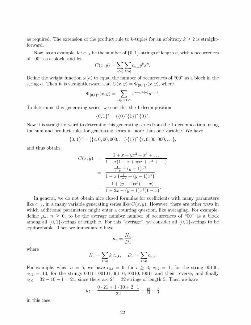
Now, as an example, let cn,k be the number of {0, 1}-strings of length n, with k occurrencesof “00” as a block, and let
C(x, y) =∑
n≥0
∑
k≥0
cn,kykxn.
Define the weight function ω(a) to equal the number of occurrences of “00” as a block in thestring a. Then it is straightforward that C(x, y) = Φ{0,1}∗(x, y), where
Φ{0,1}∗(x, y) =∑
a∈{0,1}∗
xlength(a)yω(a).
To determine this generating series, we consider the 1-decomposition
{0, 1}∗ = ({0}∗{1})∗ {0}∗.Now it is straightforward to determine this generating series from the 1-decomposition, usingthe sum and product rules for generating series in more than one variable. We have
{0, 1}∗ = ({ε, 0, 00, 000, . . .}{1})∗ {ε, 0, 00, 000, . . .},and thus obtain
C(x, y) =1 + x+ yx2 + x3 + . . .
1 − x(1 + x+ yx2 + x3 + . . .)
=1
1−x+ (y − 1)x2
1 − x(
11−x
+ (y − 1)x2)
=1 + (y − 1)x2(1 − x)
1 − 2x− (y − 1)x3(1 − x).
In general, we do not obtain nice closed formulas for coefficients with many parameterslike cn,k, in a many variable generating series like C(x, y). However, there are other ways inwhich additional parameters might enter a counting question, like averaging. For example,define µn, n ≥ 0, to be the average number number of occurrences of “00” as a blockamong all {0, 1}-strings of length n. For this “average”, we consider all {0, 1}-strings to beequiprobable. Then we immediately have
µn =Nn
Dn
,
whereNn =
∑
k≥0
k cn,k, Dn =∑
k≥0
cn,k.
For example, when n = 5, we have c5,i = 0, for i ≥ 3; c5,2 = 1, for the string 00100;c5,1 = 10, for the strings 00111, 00101, 00110, 10010, 10011 and their reverse; and finallyc5,0 = 32 − 10 − 1 = 21, since there are 25 = 32 strings of length 5. Then we have
µ5 =0 · 21 + 1 · 10 + 2 · 1
32= 12
32= 3
8
in this case.
22
12 Lecture of February 8
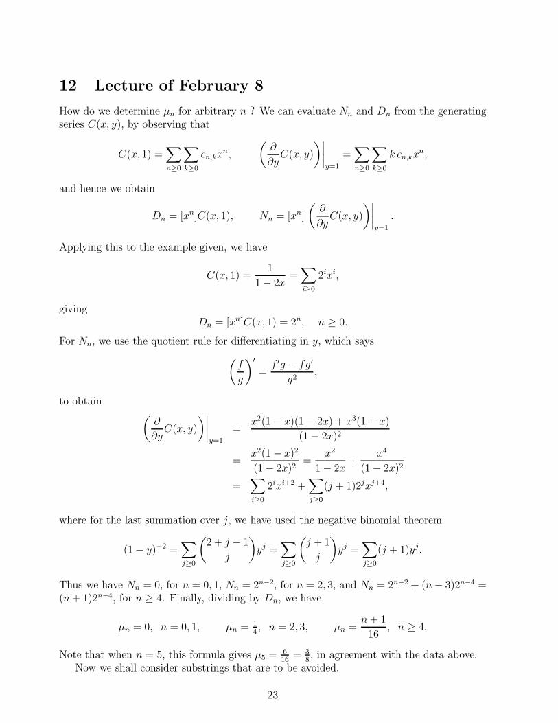
How do we determine µn for arbitrary n ? We can evaluate Nn and Dn from the generatingseries C(x, y), by observing that
C(x, 1) =∑
n≥0
∑
k≥0
cn,kxn,
(∂
∂yC(x, y)
)∣∣∣∣y=1
=∑
n≥0
∑
k≥0
k cn,kxn,
and hence we obtain
Dn = [xn]C(x, 1), Nn = [xn]
(∂
∂yC(x, y)
)∣∣∣∣y=1
.
Applying this to the example given, we have
C(x, 1) =1
1 − 2x=∑
i≥0
2ixi,
givingDn = [xn]C(x, 1) = 2n, n ≥ 0.
For Nn, we use the quotient rule for differentiating in y, which says
(f
g
)′
=f ′g − fg′
g2,
to obtain(∂
∂yC(x, y)
)∣∣∣∣y=1
=x2(1 − x)(1 − 2x) + x3(1 − x)
(1 − 2x)2
=x2(1 − x)2
(1 − 2x)2=
x2
1 − 2x+
x4
(1 − 2x)2
=∑
i≥0
2ixi+2 +∑
j≥0
(j + 1)2jxj+4,
where for the last summation over j, we have used the negative binomial theorem
(1 − y)−2 =∑
j≥0
(2 + j − 1
j
)yj =
∑
j≥0
(j + 1
j
)yj =
∑
j≥0
(j + 1)yj.
Thus we have Nn = 0, for n = 0, 1, Nn = 2n−2, for n = 2, 3, and Nn = 2n−2 + (n− 3)2n−4 =(n+ 1)2n−4, for n ≥ 4. Finally, dividing by Dn, we have
µn = 0, n = 0, 1, µn = 14, n = 2, 3, µn =
n+ 1
16, n ≥ 4.
Note that when n = 5, this formula gives µ5 = 616
= 38, in agreement with the data above.
Now we shall consider substrings that are to be avoided.
23
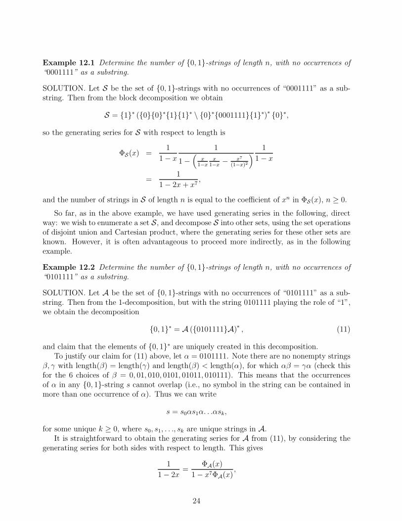
Example 12.1 Determine the number of {0, 1}-strings of length n, with no occurrences of“0001111” as a substring.
SOLUTION. Let S be the set of {0, 1}-strings with no occurrences of “0001111” as a sub-string. Then from the block decomposition we obtain
S = {1}∗ ({0}{0}∗{1}{1}∗ \ {0}∗{0001111}{1}∗)∗ {0}∗,
so the generating series for S with respect to length is
ΦS(x) =1
1 − x
1
1 −(
x1−x
x1−x
− x7
(1−x)2
) 1
1 − x
=1
1 − 2x+ x7,
and the number of strings in S of length n is equal to the coefficient of xn in ΦS(x), n ≥ 0.
So far, as in the above example, we have used generating series in the following, directway: we wish to enumerate a set S, and decompose S into other sets, using the set operationsof disjoint union and Cartesian product, where the generating series for these other sets areknown. However, it is often advantageous to proceed more indirectly, as in the followingexample.
Example 12.2 Determine the number of {0, 1}-strings of length n, with no occurrences of“0101111” as a substring.
SOLUTION. Let A be the set of {0, 1}-strings with no occurrences of “0101111” as a sub-string. Then from the 1-decomposition, but with the string 0101111 playing the role of “1”,we obtain the decomposition
{0, 1}∗ = A ({0101111}A)∗ , (11)
and claim that the elements of {0, 1}∗ are uniquely created in this decomposition.To justify our claim for (11) above, let α = 0101111. Note there are no nonempty strings
β, γ with length(β) = length(γ) and length(β) < length(α), for which αβ = γα (check thisfor the 6 choices of β = 0, 01, 010, 0101, 01011, 010111). This means that the occurrencesof α in any {0, 1}-string s cannot overlap (i.e., no symbol in the string can be contained inmore than one occurrence of α). Thus we can write
s = s0αs1α. . .αsk,
for some unique k ≥ 0, where s0, s1, . . ., sk are unique strings in A.It is straightforward to obtain the generating series for A from (11), by considering the
generating series for both sides with respect to length. This gives
1
1 − 2x=
ΦA(x)
1 − x7ΦA(x),
24
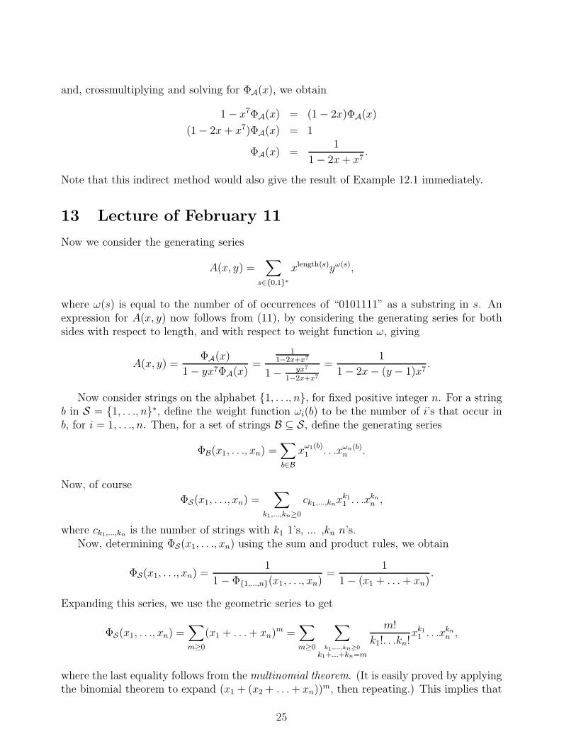
and, crossmultiplying and solving for ΦA(x), we obtain
1 − x7ΦA(x) = (1 − 2x)ΦA(x)
(1 − 2x+ x7)ΦA(x) = 1
ΦA(x) =1
1 − 2x+ x7.
Note that this indirect method would also give the result of Example 12.1 immediately.
13 Lecture of February 11
Now we consider the generating series
A(x, y) =∑
s∈{0,1}∗
xlength(s)yω(s),
where ω(s) is equal to the number of of occurrences of “0101111” as a substring in s. Anexpression for A(x, y) now follows from (11), by considering the generating series for bothsides with respect to length, and with respect to weight function ω, giving
A(x, y) =ΦA(x)
1 − yx7ΦA(x)=
11−2x+x7
1 − yx7
1−2x+x7
=1
1 − 2x− (y − 1)x7.
Now consider strings on the alphabet {1, . . ., n}, for fixed positive integer n. For a stringb in S = {1, . . ., n}∗, define the weight function ωi(b) to be the number of i’s that occur inb, for i = 1, . . ., n. Then, for a set of strings B ⊆ S, define the generating series
ΦB(x1, . . ., xn) =∑
b∈B
xω1(b)1 . . .xωn(b)
n .
Now, of course
ΦS(x1, . . ., xn) =∑
k1,...,kn≥0
ck1,...,knxk1
1 . . .xkn
n ,
where ck1,...,knis the number of strings with k1 1’s, ... ,kn n’s.
Now, determining ΦS(x1, . . ., xn) using the sum and product rules, we obtain
ΦS(x1, . . ., xn) =1
1 − Φ{1,...,n}(x1, . . ., xn)=
1
1 − (x1 + . . .+ xn).
Expanding this series, we use the geometric series to get
ΦS(x1, . . ., xn) =∑
m≥0
(x1 + . . .+ xn)m =∑
m≥0
∑
k1,...,kn≥0
k1+...+kn=m
m!
k1!. . .kn!xk1
1 . . .xkn
n ,
where the last equality follows from the multinomial theorem. (It is easily proved by applyingthe binomial theorem to expand (x1 + (x2 + . . .+ xn))m, then repeating.) This implies that
25
the number of strings in {1, . . ., n} with ki i’s, for i = 1, . . ., n, where k1, . . ., kn ≥ 0 andk1 + . . .+ kn = m, is given by
m!
k1!. . .kn!, (12)
which is usually referred to as the multinomial coefficient. Of course, it is easy to checkthat (12) is the correct cardinality for this set of strings, as follows: there are m positionsin the string (say they’re called 1, . . ., m). There are
(m
k1
)ways to choose positions for the
1’s. Then, for i = 2, . . ., n, suppose that positions have been chosen for the 1’s, ... , i− 1’s;independently of which set of k1 + · · · + ki−1 positions has been chosen for these, there are(
m−k1−···−ki−1
ki
)ways to choose positions for the i’s. Thus the total number of ways of choosing
positions for all symbols is (with convention that k0 = 0)
n∏
i=1
(m− k1 − · · · − ki−1
ki
)=
n∏
i=1
(m− k1 − · · · − ki−1)!
ki!(m− k1 − · · · − ki)!=
m!
k1!. . .kn!,
in agreement with (12).
Now let D be the set of strings (called “Smirnov” strings) on the alphabet {1, . . ., n} inwhich adjacent elements are always distinct (for example, 1342532413253435251 is in D, but134255324132 is not, because of the substring “55”). Consider an arbitrary string s ∈ S.Suppose that, for all i = 1, . . ., n, we replace each block of i’s in s by a single i. Then clearlywe obtain a unique string d ∈ D by this operation. Moreover, if we reverse this construction,then we uniquely create the strings in S if we replace each element i, i = 1, . . . , n, by a blockof i’s of any positive length, in all possible ways.
The block replacement construction above gives
ΦS(x1, . . ., xn) = ΦD(x1 + x21 + . . ., . . ., xn + x2
n + . . .) = ΦD(x1
1 − x1, . . .,
xn
1 − xn
).
Now let yi = xi/(1 − xi), for i = 1, . . ., n. Then crossmultiplying by 1 − xi and solving forxi, we obtain xi = yi/(1 + yi), for i = 1, . . ., n. This then gives
ΦD(y1, . . ., yn) = ΦS(y1
1 + y1, . . .,
yn
1 + yn
) =1
1 − y1
1+y1− . . .− yn
1+yn
,
which is the required generating series. For a consistency check on this series, note that ify1 = . . . = yn = z, then we obtain
ΦD(z, . . ., z) =1
1 − nz1+z
=1 + z
1 + z − nz
= 1 +nz
1 − (n− 1)z= 1 +
∑
k≥1
n(n− 1)k−1zk,
which simply states the obvious fact that the number of strings in D of length k is n(n−1)k−1,for k ≥ 1.
26
Another feature of the above series ΦD(y1, . . ., yn) is that it works non-commutatively.For example, expanding, we have
1
1 − y1
1+y1− . . .− yn
1+yn
= 1 +∑
k≥1
(y1
1 + y1+ . . .+
yn
1 + yn
)k
= 1 +∑
k≥1
(y1 − y2
1 + y31 − . . .+ yn − y2
n + y3n − . . .
)k.
Now the terms of total degree 1 in the yi’s are
y1 + . . .+ yn,
which checks with the fact that the strings of length 1 in D are 1, . . ., n. The terms of totaldegree 2 in the yi’s are
(y1 + . . .+ yn)(y1 + . . .+ yn) − y21 − . . .− y2
n =∑
1≤i,j≤n
i6=j
yiyj,
which correctly produces the strings of length 2 in D.
For more direct decompositions for strings on the alphabet {1, . . ., n}, for n an arbitrarypositive integer, note that the 1-decomposition extends easily, to
{1, . . ., n}∗ = {2, . . ., n}∗ ({1}{2, . . ., n}∗)∗ ,
and the block decomposition also extends easily, to
{1, . . ., n}∗ = {2, . . ., n}∗ ({1}{1}∗ ({2, . . ., n}∗ \ {ε}))∗ {1}∗.
14 Lecture of February 13
There are many examples of non-commutative results in combinatorics. For example, sup-pose that in products involving x and y we use the rule yx = qxy, where q commutes withboth x and y. Then the binomial theorem becomes
(x+ y)n =n∑
k=0
(n
k
)
q
xkyn−k, (13)
where (n
k
)
q
=
∏n
j=1(1 − qj)∏k
j=1(1 − qj)∏n−k
j=1 (1 − qj).
The polynomial(
n
k
)q
is often called the q-binomial coefficient, or Gaussian coefficient. An-
other interpretation of the expansion (13) is that(n
k
)
q
=∑
π∈Pk,n−k
qarea(π),
27
where Pk,n−k is the set of lattice paths from (0, 0) to (k, n−k), and area(π) is the area underthe path π. From a completely different point of view, in which q is a power of a prime,
(n
k
)q
is equal to the number of k-dimensional subspaces of an n-dimensional vector space overGF(q) (the finite field with q elements).
The series that we have been using are formal power series, not the power series of realvariables that have been studied in calculus courses. A formal power series is given byA(x) =
∑i≥0 aix
i, where ai = [xi]A(x), the coefficient of xi, is a complex number, for i ≥ 0.The basic rule for A(x) is that ai is determined finitely for each finite i. Let B(x) =
∑i≥0 bix
i.Then A(x) = B(x) if and only if ai = bi for all i ≥ 0, and we define sum and product by
A(x) +B(x) =∑
i≥0
(ai + bi)xi, A(x)B(x) =
∑
i≥0
(i∑
j=0
ajbi−j
)xi,
and a special case of product is the scalar product cA(x) =∑
i≥0(c ai)xi, for a complex
number c. We write A(0) = a0, and unless A is a polynomial, this is the only “evaluation”we allow. If b0 = 0, then we define the composition
A(B(x)) =∑
i≥0
aiB(x)i =∑
n≥0
∑
i≥0,j1,...,ji≥1
j1+...+ji=n
aibj1 . . .bjixn,
and note that the summations above are finite.Now suppose A(0) = 1. Then if B(x) is a multiplicative inverse of A(x), we have (since
multiplication of complex numbers is commutative, so is multiplication of A(x) with B(x),so there is no difference between a left-inverse and a right-inverse)
∑i≥0 aix
i∑
j≥0 bjxj = 1,
and equating coefficients of xn on both sides, for n ≥ 0, we obtain
b0 = 1
a1b0 + b1 = 0
a2b0 + a1b1 + b2 = 0,
where the nth equation is anb0+an−1b1+. . .+b0 = 0, n ≥ 1. But this gives b0 = 1, and allowsus to determine bn uniquely in terms of b0, . . ., bn−1, for each n ≥ 1, so, by induction on n,B(x) is unique. Applying this process to obtain the multiplicative inverse of A(x) = 1 − x,we obtain bn = 1, n ≥ 0, by induction on n, or (1 − x)−1 =
∑i≥0 x
i. But substitution intothis, for an arbitrary A(x) with A(0) = 1, gives
A(x)−1 = (1 − (1 −A(x)))−1 = 1 +∑
i≥1
(1 −A(x))i ,
which is therefore the unique multiplicative inverse of A(x).
We define differentiation and integration operators by
d
dxA(x) =
∑
i≥1
iaixi−1, IxA(x) =
∑
i≥0
ai
i+ 1xi+1.
Now note that we have uniqueness for solution of differential equations: if ddxA(x) = d
dxB(x)
and A(0) = B(0), then A(x) = B(x).
28
15 Lecture of February 15
Now
d
dx(A(x) +B(x)) =
∑
i≥1
i(ai + bi)xi−1 =
∑
i≥1
iaixi−1 +
∑
i≥1
ibixi−1 =
d
dxA(x) +
d
dxB(x),
so this differentiation operator satisfies the sum rule, and
d
dx(A(x)B(x)) =
∑
i≥1
i∑
j=0
iajbi−jxi−1
=∑
i≥1
i∑
j=0
(j + i− j)ajbi−jxi−1
=
(d
dxA(x)
)B(x) + A(x)
(d
dxB(x)
),
and differentiation satisfies the product rule. Induction on n then gives ddxB(x)n = nB(x)n−1 d
dxB(x)
for positive integers n, which allows us to prove the chain rule:
d
dxA(B(x)) = A′(B(x))
d
dxB(x).
We now define three special series
ε(x) =∑
n≥0
1
n!xn, λ(x) =
∑
n≥1
1
nxn, Ba(x) =
∑
n≥0
a(a− 1). . .(a− n+ 1)
n!xn,
where a is a complex number parameter in Ba(x). Our object is to show that ε(x), λ(x), Ba(x)have the properties of the familiar functions ex, ln(1 − x)−1, (1 + x)a, respectively. (Exceptthat we will NOT be able to consider, for example, ε(ε(x)), since it uses composition witha series with constant term 1.) First, note that d
dxε(x) = ε(x). Then, for example, we can
prove that ε(x)ε(−x) = 1, since ε(x)ε(−x) has constant term ε(0)ε(−0) = 1, and
d
dx(ε(x)ε(−x)) = ε(x)ε(−x) − ε(x)ε(−x) = 0,
where we have used the product rule and chain rule. The result follows by the uniqueness ofsolution of differential equations ( since 1 also has constant term 1 and derivative 0). Also,we have d
dxλ(x) =
∑n≥0 x
n = (1 − x)−1, so
d
dx(λ(1 − ε(−x))) = (ε(−x))−1 ε(−x) = 1,
by the chain rule, and λ(1 − ε(−0)) = 0, and we conclude that λ(1 − ε(−x)) = x, byuniqueness of solution of differential equations. (The series 1 − ε(−x) has constant term 0,
29
so the composition λ(1 − ε(−x)) is valid.) Similarly, we prove that ε(λ(x)) = (1 − x)−1,using ε(λ(0)) = 1, and
d
dx((1 − x)ε(λ(x))) = −ε(λ(x)) + (1 − x)ε(λ(x))(1 − x)−1 = 0,
using the product rule and chain rule. For the series Ba(x), we have ddxBa(x) = aBa−1(x),
and we omit further details of these computations.Now, it is easy to verify that there are no zero divisors for formal power series, and this
fact allows us to establish that nth roots are unique, at least with given constant term, asfollows. Suppose A(0) = B(0) = 1, and A(x)n = B(x)n, for some positive integer n. Thenwe have
0 = A(x)n −B(x)n = (A(x) −B(x))(A(x)n−1 + A(x)n−2B(x) + . . .+B(x)n−1).
Now the constant term in the second factor is A(0)n−1 + A(0)n−2B(0) + . . . + B(0)n−1 =n 6= 0, so we conclude that A(x) − B(x) = 0, since there are no zero divisors, which givesA(x) = B(x), as required. But we can determine the nth root of A(x) with A(0) = 1 bysubstitution in the binomial series Ba(x), to obtain
A(x)1n = (1 + (A(x) − 1))
1n = 1 +
∑
i≥1
1n( 1
n− 1). . .( 1
n− i+ 1)
i!(A(x) − 1)i ,
which is therefore the unique nth root with constant term 1.
We introduce trigonometric series by defining
sin(x) = x− x3
3!+x5
5!− . . ., cos(x) = 1 − x2
2!+x4
4!− . . .,
and then proving the properties of these series from properties of the series ε(x) = ex, by
sin(x) =eix − e−ix
2i, cos(x) =
eix + e−ix
2,
so, for example, we have
sin(x)2 + cos(x)2 =
(eix − e−ix
2i
)2
+
(eix + e−ix
2
)2
= 14
(−(e2ix − 2 + e−2ix) + (e2ix + 2 + e−2ix)
)= 1.
Then, noting that cos(x) has constant term 1, so it is invertible, we define
tan(x) =sin(x)
cos(x)= x+
x3
3+
2x5
15+ . . . = x+
2x3
3!+
16x5
5!+ . . .,
sec(x) =1
cos(x)= 1 +
x2
2+
5x4
24+ . . . = 1 +
x2
2!+
5x4
4!+ . . ..
30
Finally, we are going to show that the sequences 1, 2, 16, . . . and 1, 1, 5, . . ., which are thecoefficients in tan(x) and sec(x), scaled by the factorial, count some interesting combinatorialobjects.
Let a2k+1, for k ≥ 0, denote the number of permutations σ1. . .σ2k+1 of {1, . . ., 2k + 1},for which σ1 < σ2 > σ3 < . . . < σ2k > σ2k+1. Similarly, let b2k, for k ≥ 0, denote the numberof permutations σ1. . .σ2k of {1, . . ., 2k}, for which σ1 < σ2 > σ3 < . . . > σ2k−1 < σ2k. Thesepermutations are called alternating permutations. For example, a1 = 1 (the permutationhere is 1), a3 = 2 (the permutations are 132, 231), b0 = 1 (the empty permutation ε), b2 = 1(the permutation 12), and b4 = 5 (the permutations 1423, 2413, 3412, 1324, 2314). Toobtain a recurrence equation for these numbers, first consider an alternating permutation on{1, . . ., 2k + 1}, where k ≥ 1. Then we have σ2i+2 = 2k + 1 for some unique i = 0, . . ., k − 1.In this case, σ1. . .σ2i+1 is an alternating permutation on some (2i+1)-subset α of {1, . . ., 2k},and σ2i+3. . .σ2k+1 is an alternating permutation on {1, . . ., 2k} \ α. Then there are
(2k
2i+1
)
choices for α, and for each such α, a2i+1 choices for σ1. . .σ2i+1, and a2k−2i−1 choices forσ2i+3. . .σ2k+1. Moreover, this is bijective, and we conclude that
a2k+1 =k−1∑
i=0
(2k
2i+ 1
)a2i+1a2k−2i−1, k ≥ 1, (14)
with initial condition a1 = 1. Similarly, we obtain
b2k =k−1∑
i=0
(2k
2i+ 1
)a2i+1b2k−2i−2 k ≥ 1, (15)
with initial condition b0 = 1. Now let
A(x) =∑
k≥0
a2k+1x2k+1
(2k + 1)!, B(x) =
∑
k≥0
b2k
x2k
(2k)!,
which are called the exponential generating series for the sequences {a2k+1}k≥0, {b2k}k≥0,
respectively. Now, multiply both sides of (14) by x2k
(2k)!, and sum for k ≥ 1, to obtain
∑
k≥1
a2k+1x2k
(2k)!=∑
k≥1
k−1∑
i=0
a2i+1
(2i+ 1)!
a2k−2i−1
(2k − 2i− 1)!x2k.
Then change indices in the double summation from i, k to i, j, where j = k − 1 − i. Thisgives ranges of summation i ≥ 0 and j ≥ 0, and we have 2k = 2(i+ j + 1) = 2i+ 1 + 2j+ 1,so the above equation becomes
∑
k≥1
a2k+1x2k
(2k)!=∑
i≥0
a2i+1
(2i+ 1)!x2i+1
∑
j≥0
a2j+1
(2j + 1)!x2j+1.
Translating this in terms of A(x), we obtain
d
dx(A(x) − a1x) = A(x)2,
31
sod
dxA(x) = 1 + A(x)2.
(In CO 330, exponential generating series are considered in greater detail. There we givea product rule that allows us to write down the above differential equation immediately,avoiding all the details of summation indices, etc.) To solve this differential equation, divideboth sides by 1 + A(x)2 (this has constant term 1, so it is invertible), and integrate withrespect to x, to obtain
arctan(A(x)) = x+ c,
where we determine from the initial condition A(0) = 0 that c = 0, and conclude thatA(x) = tan(x).
Similarly, from (15), multiplying by x2k
(2k)!, and summing for k ≥ 1, we obtain
d
dxB(x) = A(x)B(x).
To solve this differential equation, divide both sides by B(x) (this has constant term 1, so itis invertible), and integrate with respect to x, to obtain
ln(B(x)) = ln(sec(x)) + c,
where we determine from the initial condition B(0) = 1 that c = 0, and conclude thatB(x) = sec(x).
There are many other types of generating series used for various types of applications.For this reason, the generating series
∑n≥0 anx
n that we have used in MATH 249 is oftenreferred to as the ordinary generating series for the sequence {an}n≥0. For example, innumber theoretic applications, the Dirichlet generating series
∑n≥1 an n
−s is often used(here s is the variable). The significance of each choice of generating series is usually to befound in their product. For example, we have
∑
i≥0
aixi∑
j≥0
bjxj =
∑
n≥0
∑
i,j≥0i+j=n
aibj
xn,
∑
i≥0
ai
xi
i!
∑
j≥0
bjxj
j!=∑
n≥0
∑
i,j≥0i+j=n
(n
i
)aibj
xn
n!,
∑
i≥1
ai i−s∑
j≥1
bj j−s =
∑
n≥1
∑
i,j≥1i·j=n
aibj
n−s.
As an extra, the following example gives the general solution technique for the enumer-ation of strings excluding arbitrary substrings (that may overlap with themselves).
32
Example Find the number of {0, 1}-strings of length n, with no occurrences of 01101 as asubstring.
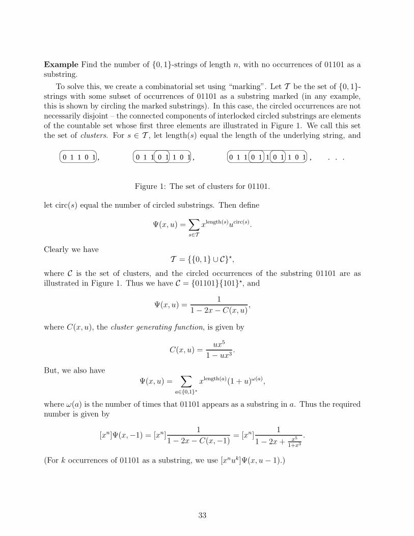
To solve this, we create a combinatorial set using “marking”. Let T be the set of {0, 1}-strings with some subset of occurrences of 01101 as a substring marked (in any example,this is shown by circling the marked substrings). In this case, the circled occurrences are notnecessarily disjoint – the connected components of interlocked circled substrings are elementsof the countable set whose first three elements are illustrated in Figure 1. We call this setthe set of clusters. For s ∈ T , let length(s) equal the length of the underlying string, and
0 1 1 0 1 , 0 1 1 0 1 1 0 1 , 0 1 1 0 1 1 0 1 1 0 1 , . . .
Figure 1: The set of clusters for 01101.
let circ(s) equal the number of circled substrings. Then define
Ψ(x, u) =∑
s∈T
xlength(s)ucirc(s).
Clearly we haveT = {{0, 1} ∪ C}⋆,
where C is the set of clusters, and the circled occurrences of the substring 01101 are asillustrated in Figure 1. Thus we have C = {01101}{101}⋆, and
Ψ(x, u) =1
1 − 2x− C(x, u),
where C(x, u), the cluster generating function, is given by
C(x, u) =ux5
1 − ux3.
But, we also have
Ψ(x, u) =∑
a∈{0,1}∗
xlength(a)(1 + u)ω(a),
where ω(a) is the number of times that 01101 appears as a substring in a. Thus the requirednumber is given by
[xn]Ψ(x,−1) = [xn]1
1 − 2x− C(x,−1)= [xn]
1
1 − 2x+ x5
1+x3
.
(For k occurrences of 01101 as a substring, we use [xnuk]Ψ(x, u− 1).)
33
16 Lecture of February 25
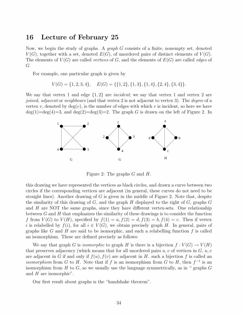
Now, we begin the study of graphs. A graph G consists of a finite, nonempty set, denotedV (G), together with a set, denoted E(G), of unordered pairs of distinct elements of V (G).The elements of V (G) are called vertices of G, and the elements of E(G) are called edges ofG.
For example, one particular graph is given by
V (G) = {1, 2, 3, 4}, E(G) = {{1, 2}, {1, 3}, {1, 4}, {2, 4}, {3, 4}}.
We say that vertex 1 and edge {1, 2} are incident; we say that vertex 1 and vertex 2 arejoined, adjacent or neighbours (and that vertex 2 is not adjacent to vertex 3). The degree of avertex v, denoted by deg(v), is the number of edges with which v is incident, so here we havedeg(1)=deg(4)=3, and deg(2)=deg(3)=2. The graph G is drawn on the left of Figure 2. In
G G H
1 2
34
1
4
2 3
a
b
c
d
Figure 2: The graphs G and H .
this drawing we have represented the vertices as black circles, and drawn a curve between twocircles if the corresponding vertices are adjacent (in general, these curves do not need to bestraight lines). Another drawing of G is given in the middle of Figure 2. Note that, despitethe similarity of this drawing of G, and the graph H displayed to the right of G, graphs Gand H are NOT the same graphs, since they have different vertex-sets. One relationshipbetween G and H that emphasizes the similarity of these drawings is to consider the functionf from V (G) to V (H), specified by f(1) = a, f(2) = d, f(3) = b, f(4) = c. Then if vertexi is relabelled by f(i), for all i ∈ V (G), we obtain precisely graph H . In general, pairs ofgraphs like G and H are said to be isomorphic, and such a relabelling function f is calledan isomorphism. These are defined precisely as follows:
We say that graph G is isomorphic to graph H is there is a bijection f : V (G) → V (H)that preserves adjacency (which means that for all unordered pairs u, v of vertices in G, u, vare adjacent in G if and only if f(u), f(v) are adjacent in H . such a bijection f is called anisomorphism from G to H . Note that if f is an isomorphism from G to H , then f−1 is anisomorphism from H to G, so we usually use the language symmetrically, as in “ graphs Gand H are isomorphic”.
Our first result about graphs is the “handshake theorem”.
34
Theorem 16.1 ∑
v∈V (G)
deg(v) = 2 |E(G)|
PROOF. Count the (vertex, edge) pairs that are incident. There are deg(v) such pairs foreach vertex v, giving the lefthandside, and there are two such pairs for each edge, giving therighthandside.
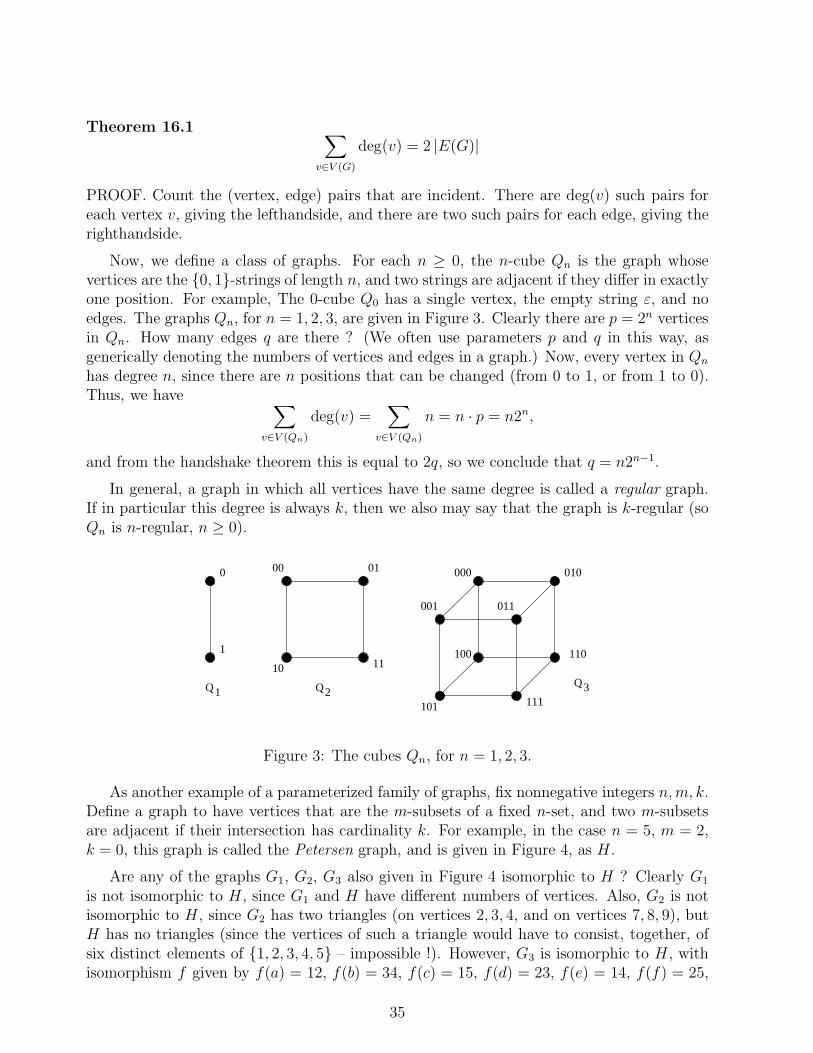
Now, we define a class of graphs. For each n ≥ 0, the n-cube Qn is the graph whosevertices are the {0, 1}-strings of length n, and two strings are adjacent if they differ in exactlyone position. For example, The 0-cube Q0 has a single vertex, the empty string ε, and noedges. The graphs Qn, for n = 1, 2, 3, are given in Figure 3. Clearly there are p = 2n verticesin Qn. How many edges q are there ? (We often use parameters p and q in this way, asgenerically denoting the numbers of vertices and edges in a graph.) Now, every vertex in Qn
has degree n, since there are n positions that can be changed (from 0 to 1, or from 1 to 0).Thus, we have ∑
v∈V (Qn)
deg(v) =∑
v∈V (Qn)
n = n · p = n2n,
and from the handshake theorem this is equal to 2q, so we conclude that q = n2n−1.
In general, a graph in which all vertices have the same degree is called a regular graph.If in particular this degree is always k, then we also may say that the graph is k-regular (soQn is n-regular, n ≥ 0).
Q Q Q321
0
1
00 01
10 11
000 010
110100
001 011
101 111
Figure 3: The cubes Qn, for n = 1, 2, 3.
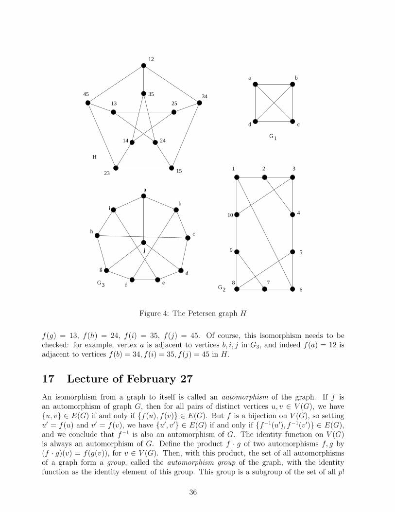
As another example of a parameterized family of graphs, fix nonnegative integers n,m, k.Define a graph to have vertices that are the m-subsets of a fixed n-set, and two m-subsetsare adjacent if their intersection has cardinality k. For example, in the case n = 5, m = 2,k = 0, this graph is called the Petersen graph, and is given in Figure 4, as H .
Are any of the graphs G1, G2, G3 also given in Figure 4 isomorphic to H ? Clearly G1
is not isomorphic to H , since G1 and H have different numbers of vertices. Also, G2 is notisomorphic to H , since G2 has two triangles (on vertices 2, 3, 4, and on vertices 7, 8, 9), butH has no triangles (since the vertices of such a triangle would have to consist, together, ofsix distinct elements of {1, 2, 3, 4, 5} – impossible !). However, G3 is isomorphic to H , withisomorphism f given by f(a) = 12, f(b) = 34, f(c) = 15, f(d) = 23, f(e) = 14, f(f) = 25,
35
12
34
1523
45 35
24
13 25
14
H
G1
G3 G2
a b
cd
1 2 3
4
5
678
9
10
a
b
c
d
ef
g
h
i
j
Figure 4: The Petersen graph H
f(g) = 13, f(h) = 24, f(i) = 35, f(j) = 45. Of course, this isomorphism needs to bechecked: for example, vertex a is adjacent to vertices b, i, j in G3, and indeed f(a) = 12 isadjacent to vertices f(b) = 34, f(i) = 35, f(j) = 45 in H .
17 Lecture of February 27
An isomorphism from a graph to itself is called an automorphism of the graph. If f isan automorphism of graph G, then for all pairs of distinct vertices u, v ∈ V (G), we have{u, v} ∈ E(G) if and only if {f(u), f(v)} ∈ E(G). But f is a bijection on V (G), so settingu′ = f(u) and v′ = f(v), we have {u′, v′} ∈ E(G) if and only if {f−1(u′), f−1(v′)} ∈ E(G),and we conclude that f−1 is also an automorphism of G. The identity function on V (G)is always an automorphism of G. Define the product f · g of two automorphisms f, g by(f · g)(v) = f(g(v)), for v ∈ V (G). Then, with this product, the set of all automorphismsof a graph form a group, called the automorphism group of the graph, with the identityfunction as the identity element of this group. This group is a subgroup of the set of all p!
36

bijections on V (G) (where |V (G)| = p). Among other consequences, this implies that thenumber of automorphisms of a graph divides p!. For example, how many automorphismsdoes the graph G in Figure 5 have ? The answer is 2, with the identity function giving one
G
1
2
3
45
Figure 5: The graph G.
automorphism, and the function f(1) = 3, f(2) = 2, f(3) = 1, f(4) = 5, f(5) = 4 giving theother. (It is straightforward to check that f is an automorphism. To prove that there areno other automorphisms, note that vertices 1 and 3 have degree 3, but vertices 2, 4, 5 havedegree 2, so every automorphism must map 1, 3 to 1, 3 only, in either order; once this orderis given, then 2, 4, 5 are mapped to 2, 4, 5 in one way only.)
What is the largest number of automorphisms that a graph on p vertices can have ? Theanswer is p!, for either the complete graph Kp on p vertices, in which every pair of verticesis adjacent, or the empty graph Z, with no edges. For p = 5, these are given in Figure 6.
K5 Z
Figure 6: Graphs on 5 vertices with 5! automorphisms.
The relationship between K5 and Z above is generalized by defining the complement ofa graph. The complement G of a graph G is the graph with vertex set V (G), and whoseedges are the unordered pairs of vertices that are NOT in E(G). For example, in Figure 6,
K5 = Z, and Z = K5. Now, in general, G and G have exactly the same automorphisms (thisis easy to prove, since a pair of vertices is adjacent in G if and only if it is not adjacent inG). One use of this result is to count automorphisms for a graph whose complement is mucheasier to handle. For example, consider the graph G given in Figure 7. The complement ofG is H , given beside G in Figure 7. But it is easy to see that H has exactly 6 · 4 · 2 = 48automorphisms, since 1 can be mapped to any of the 6 vertices, but then 3 must be mappedto the vertex that is adjacent to the image of 1; then 2 can be mapped to any of the 4remaining vertices, but then 5 must be mapped to the vertex that is adjacent to the image
37
GH
1
2
3
4
5
6
1
2
3
4
5
6
Figure 7: A graph G, and its complement H .
of 2; finally 4 can be mapped to any of the 2 remaining vertices, but then 6 must be mappedto the vertex that is adjacent to the image of 4.
A graph G is vertex transitive if, for every pair u, v of vertices in G, there exists anautomorphism f such that f(u) = v. (Note: In general, the choice of f will depend onu, v.) A graph G is edge transitive if, for every pair {u, v}, {x, y} of edges in G, there existsan automorphism f such that either f(u) = x, f(v) = y or f(u) = y, f(v) = x. It followsimmediately that a vertex transitive graph must be regular. Does vertex transitivity implyedge transitivity or vice-versa ? Consider the graphs in Figure 8. Note that graphs G1 and
G1
G2
G3G4
Figure 8: The graphs Gi, i = 1, . . ., 4.
G2 are both regular, but neither are vertex transitive. For G1, no automorphism can map
38
any vertex on the triangle to any vertex on the square. For G2, there are precisely twotriangles, at the top and bottom, so no automorphism can map any of the 6 vertices onthese triangles to any of the two remaining vertices.
Now, graph G3 is edge transitive, but not vertex transitive (also, G3 is not regular). Wewrite G3 as K4,3, since it has a complete set of edges between the 4-set of vertices at the topand the 3-set of vertices at the bottom.
Finally, graph G4 is vertex transitive, but it is not edge transitive, since the three hori-zontal edges are not contained in any triangle.
18 Lecture of February 29
A subgraph H of a graph G is a graph whose vertex set is a nonempty subset of V (G), andedge set is a subset of the edges of G joining two vertices in V (H). A spanning subgraph Hof G has V (H) = V (G). An induced subgraph of G has vertex set that is a nonempty subsetof V (G), and edge set consisting of all the edges of G joining two vertices in V (H).
A walk in a graph G is a sequence v0e1v1. . .envn, n ≥ 0, in which v0, v1, . . ., vn are verticesof G, and e1, . . ., en are edges of G, with ei = {vi−1, vi} for i = 1, . . ., n. This walk is fromv0 to vn, and has length n. Note that we can reverse a walk, so that vnen. . .v1e1v0 is then awalk from vn to v0, and we therefore often speak of a walk between a pair of vertices. A pathis a walk in which the vertices are distinct.
Note that if there is a walk from vertex u to vertex v in a graph G, then there is a pathfrom u to v in G, by the following argument: let the vertices on the walk be v0v1. . .vn, wherev0 = u, vn = v. Then if no vertex appears more than once, it is a path, and we are done.Otherwise, there exists i < j with vi = vj , and in this case, v0v1. . .vivj+1. . .vn is a shorterwalk from u to v. Continue until we have a path (n is finite, and G has a finite number ofvertices, edges, so this is a finite procedure.)
Now, given a graph G, define the relation PG on V (G) by uPGv if there is a path in Gfrom u to v.
Theorem 18.1 For any graph G, PG is an equivalence relation.
PROOF. The relation is reflexive, since v is a path of length 0 from v to v, for all v ∈ V (G)(so we have vPGv). The relation is symmetric, since if v0v1. . .vn is a path from u = v0 tov = vn, then vn. . .v1v0 is a path from v = vn to u = v0, for all u, v ∈ V (G) (so we have uPGvimplies vPGu). The relation is transitive, since if there is a path x0. . .xn from u to v in G(with u = x0, v = xn), and there is a path y0. . .ym from v to w in G (with v = y0, w = ym),then x0. . .xny1. . .ym is a walk from u to w in G, but the result above then implies that thereis a path from u to w ( so we have uPGv and vPGw implies uPGw).
Of course, an equivalence relation partitions the set on which it is defined into equivalenceclasses (which means that uPGv if and only if u and v are in the same equivalence class).We define a graph G to be connected if PG has a single equivalence class. In general, theinduced subgraph whose vertex set is an equivalence class is called a (connected) component
39
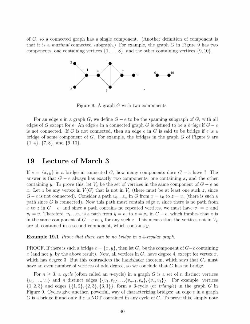
of G, so a connected graph has a single component. (Another definition of component isthat it is a maximal connected subgraph.) For example, the graph G in Figure 9 has twocomponents, one containing vertices {1, . . ., 8}, and the other containing vertices {9, 10}.
1
2
3
4
5
6
78 9 10
G
Figure 9: A graph G with two components.
For an edge e in a graph G, we define G− e to be the spanning subgraph of G, with alledges of G except for e. An edge e in a connected graph G is defined to be a bridge if G− eis not connected. If G is not connected, then an edge e in G is said to be bridge if e is abridge of some component of G. For example, the bridges in the graph G of Figure 9 are{1, 4}, {7, 8}, and {9, 10}.
19 Lecture of March 3
If e = {x, y} is a bridge in connected G, how many components does G − e have ? Theanswer is that G − e always has exactly two components, one containing x, and the othercontaining y. To prove this, let Vx be the set of vertices in the same component of G− e asx. Let z be any vertex in V (G) that is not in Vx (there must be at least one such z, sinceG− e is not connected). Consider a path v0. . .vn in G from x = v0 to z = vn (there is such apath since G is connected). Now this path must contain edge e, since there is no path fromx to z in G − e, and since a path contains no repeated vertices, we must have v0 = x andv1 = y. Therefore, v1. . .vn is a path from y = v1 to z = vn in G− e, which implies that z isin the same component of G− e as y for any such z. This means that the vertices not in Vx
are all contained in a second component, which contains y.
Example 19.1 Prove that there can be no bridge in a 4-regular graph.
PROOF. If there is such a bridge e = {x, y}, then letGx be the component ofG−e containingx (and not y, by the above result). Now, all vertices in Gx have degree 4, except for vertex x,which has degree 3. But this contradicts the handshake theorem, which says that Gx musthave an even number of vertices of odd degree, so we conclude that G has no bridge.
For n ≥ 3, a cycle (often called an n-cycle) in a graph G is a set of n distinct vertices{v1, . . ., vn} and n distinct edges {{v1, v2}, . . .{vn−1, vn}, {vn, v1}}. For example, vertices{1, 2, 3} and edges {{1, 2}, {2, 3}, {3, 1}}, form a 3-cycle (or triangle) in the graph G inFigure 9. Cycles give another, powerful, way of characterizing bridges: an edge e in a graphG is a bridge if and only if e is NOT contained in any cycle of G. To prove this, simply note
40
that a cycle containing edge e = {x, y} consists of edge {x, y}, together with a path fromx to y in G − e, in which case e is not a bridge. For example, this characterization can bechecked for the three bridges in the graph G in Figure 9.
We begin with another lemma about cycles. Suppose that there are two different pathsbetween some pair of distinct vertices in a graph G. Then G must contain a cycle. To provethis suppose the paths are P1 = u0. . .um, and P2 = v0. . .vn, where u0 = v0, and um = vn. Leti ≥ 0 be the smallest value for which ui+1 6= vi+1 (so u0 = v0, . . ., ui = vi). There must besuch an i, since the paths are different. Let j be the smallest value, with j > i, for which uj
is contained in P2, and suppose that uj = vk. There must be such a j, since um is containedin P2. Then uiui+1. . .ujvk−1. . .vi+1 is a cycle in G, proving the result.
A tree is a connected graph with no cycles. Since it is connected, a tree must contain atleast one path between every pair of vertices, but the above result implies that there cannotbe more than one path between any pair of vertices (otherwise, we would have a cycle). Thuswe conclude that there is a unique path between every pair of vertices in a tree. Also, sinceno edge in a tree is contained in a cycle, our cycle characterization of bridges implies thatin a tree, every edge is a bridge.
Every tree on p vertices has q = p − 1 edges, for p ≥ 1. We prove this by (strong)induction on p. For the base case, there is only one tree for p = 1, which has 0 edges (thisis connected, with no cycles), so the result is true for p = 1. For the induction hypothesis,with p > 1, assume that the result holds for values smaller than p, and consider an arbitrarytree T on p vertices. Now T has at least one edge (otherwise, it is not connected, since itwould have p > 1 components). Remove an arbitrary edge e = {x, y} from T . We haveproved above that e is a bridge, so T − e has two components, with one containing vertex x,and the other containing vertex y. There can be no cycles in T − e, since T has no cycles,so both components of T − e are trees. Let T1 be the component of T − e containing x, andT2 be the component containing y. Let pi be the number of vertices in Ti, for i = 1, 2. Thenwe have p1, p2 ≥ 1, and p1 + p2 = p, so p1, p2 ≤ p− 1, and we can thus apply the inductionhypothesis to determine that the number of edges in Ti is pi − 1, for i = 1, 2. Then thenumber of edges in T is given by
(p1 − 1) + (p2 − 1) + 1 = p1 + p2 − 1 = p− 1,
and we have proved that the result is true for T . The result has now been established for allp ≥ 1, by mathematical induction.
A spanning tree of a graph is a spanning subgraph that is a tree.
Theorem 19.2 A graph G is connected if and only if it has a spanning tree T .
PROOF. If G has a spanning tree T , then T contains a unique path between every pair ofvertices, and all such paths are contained in G, implying that G is connected.
For the converse, suppose that G is connected. If G has no cycle, then G is itself a tree,and so has a spanning tree. Otherwise, if G has a cycle, remove an arbitrary edge e on anycycle of G. Now, from the cycle characterization of bridges, e is not a bridge, so G − e isa spanning subgraph of G that is connected, and has one fewer edge than G. Repeat thisfinite process, until there is no cycle, to obtain a spanning tree of G.
41
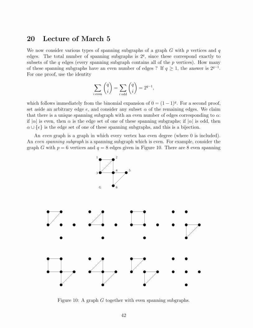
20 Lecture of March 5
We now consider various types of spanning subgraphs of a graph G with p vertices and qedges. The total number of spanning subgraphs is 2q, since these correspond exactly tosubsets of the q edges (every spanning subgraph contains all of the p vertices). How manyof these spanning subgraphs have an even number of edges ? If q ≥ 1, the answer is 2q−1.For one proof, use the identity
∑
i even
(q
i
)=∑
i odd
(q
i
)= 2q−1,
which follows immediately from the binomial expansion of 0 = (1− 1)q. For a second proof,set aside an arbitrary edge e, and consider any subset α of the remaining edges. We claimthat there is a unique spanning subgraph with an even number of edges corresponding to α:if |α| is even, then α is the edge set of one of these spanning subgraphs; if |α| is odd, thenα ∪ {e} is the edge set of one of these spanning subgraphs, and this is a bijection.
An even graph is a graph in which every vertex has even degree (where 0 is included).An even spanning subgraph is a spanning subgraph which is even. For example, consider thegraph G with p = 6 vertices and q = 8 edges given in Figure 10. There are 8 even spanning
1 2
34 5
6G
Figure 10: A graph G together with even spanning subgraphs.
42
subgraphs of G, also given in Figure 10, below G itself.For any field F and positive integer q, the set Fq, consisting of q-tuples of elements of F, is a
vector space of dimension q. This vector space is also given by span{(1, 0, . . ., 0), (0, 1, 0, . . ., 0),. . ., (0, . . ., 0, 1)}, where 0 and 1 are the additive identity and multiplicative identity in thefield, respectively. In this course, we consider the field Z2 = {0, 1} of integers modulo 2.
Consider a graph G with q edges, where we index the edges e1, . . ., eq in an arbitrary,but fixed, way. The incidence vector of a spanning subgraph of G is a {0, 1} q-tuple, with1 in entry i if ei is contained in the subgraph, and 0 otherwise, for each i = 1, . . ., q. Usingincidence vectors, we associate a unique element of Zq
2 with each spanning subgraph of G.The 0-vector (0, . . ., 0) is the incidence vector of the spanning subgraph with no edges, and wedenote this graph by Z. Now, to understand what the vector space operations on incidencevectors mean for the underlying spanning subgraphs themselves: for scalar multiples of aspanning subgraph H , we have 1H = H , since scalar multiplication of the incidence vectorby 1 doesn’t change any of the entries; we also have 0H = Z, since scalar multiplication ofthe incidence vector by 0 makes all of the entries 0. For spanning subgraphs H1, H2, thesum H1 + H2 is the spanning subgraph whose edge set is the symmetric difference of theedge sets of H1 and H2 – i.e., it has all the edges that are contained in exactly one of H1 andH2, which exactly mimics the sums in Z2 that are carried out in each entry. Thus we referto the set of spanning subgraphs of a graph as the edge space of the graph.
We now consider two subspaces of the edge space.
Theorem 20.1 For any graph G with q edges, the set of spanning subgraphs with an evennumber of edges is a (q − 1)-dimensional subspace of the edge space of G (the vector spaceof spanning subgraphs).
SOLUTION. The set of incidence vectors vt = (v1, . . ., vq)t (regarding them as column
vectors) for these spanning subgraphs is exactly the null space of the 1 × q matrix A =(1 1 . . .1). We recall from linear algebra, that this is always a vector space over the samefield as the entries of A. (PROOF: If A is m × n, then its null space consists of all n × 1vectors x such that Ax = 0, where 0 is m×1. Thus the null space contains 0n×1, and is thusnonempty. It is closed under scalar multiplication by the field element c, since for x in thenull space we have
Acx = cAx = c 0 = 0.
The null space is also closed under vector addition, since for x, y in the null space, we have
A(x+ y) = Ax+ Ay = 0 + 0 = 0.
Thus the null space of A is a subspace of Fn (as column vectors), and is thus a vector spaceover F.)
Since the matrix A has rank 1, then the null space has dimension q−1 (rank plus nullityequals number of columns). As in our linear algebra courses, we determine the null space byconsidering the linear equation
v1 + v2 + . . .+ vq = 0,
43
and setting v2, . . ., vq as arbitrary parameters in Z2. Thus we have v1 = −v2 − . . . − vq =v2 + . . .+ vq, so the null space is given by
{(v2 + . . .+ vq, v2, . . ., vq)t : v2, . . ., vq ∈ Z2}
= span{(1, 1, 0, . . ., 0)t, (1, 0, 1, 0, . . ., 0)t, . . .(1, 0, . . ., 0, 1)t},where, of course, these q − 1 vectors are linearly independent. Note that the first entry inthese vectors acts as a parity check.
We could also establish the above result more directly, instead of recognizing the set asthe null space of a particular matrix A, by proving that the set is a nonempty subset of theedge space that is closed under scalar multiplication and vector addition. Indeed, we use thismethod of proof for the following result, concerning the second subspace of the edge space.
Theorem 20.2 For any graph G with q edges, the set C(G) of even spanning subgraphs isa subspace of the edge space of G.
SOLUTION. The set C(G) contains the subgraph Z, with no edges, since this subgraph hasdegree 0 at every vertex. Then for H ∈ C(G), we have 0H = Z ∈ C(G), and 1H = H ∈C(G), so C(G) is closed under scalar multiplication. Now, for H1, H2 ∈ C(G), we considerH1 +H2: for an arbitrary vertex v ∈ G, suppose that v has degree 2k in H1, and degree 2min H2, and that exactly n of the edges incident with v in H1 are also contained in H2; thenthe degree of vertex v in H1 +H2 is given by 2k + 2m− 2n, which is even, and we concludethat H1 + H2 ∈ C(G), so C(G) is closed under addition. Thus C(G) is a subspace, givingthe result.
To determine the dimension of the subspace C(G), we consider first the case in which Gis connected. Since G is connected, it must have a spanning tree, so let T be an arbitrary,but fixed spanning tree of G. We refer to the edges of G that are contained in T as treeedges, and the edges of G that are not contained in T as nontree edges.
For H1, H2 ∈ C(G), suppose that H1, H2 have exactly the same sets of nontree edges.Then all edges of H1 +H2 are tree edges, so all components of H1 +H2 are trees (containedin T ).
21 Lecture of March 7
In a tree on p ≥ 2 vertices, there must be at least two vertices of degree 1. To prove this,consider a longest path u0. . .um in the tree. Since p ≥ 2, we must have m ≥ 1, since everyedge would give a path of length 1, and a graph on p vertices and 0 edges has p components(and thus is not connected for p ≥ 2). Now, u0 is adjacent to u1. If u0 is adjacent to uj forany j ≥ 2, then u0. . .uj is a cycle in the tree, which is impossible. If u0 is adjacent to v forany vertex v in the tree that is not contained in the longest path, then vu0. . .um is a path inthe tree that is longer than the longest path, which is impossible. Therefore, u0 is adjacentonly to vertex u1 in the tree, and so has degree 1. The same argument proves that um hasdegree 1, so we have constructed two vertices of degree 1, proving the result.
44
Thus, returning to the argument at the end of the previous class, if any of the componentsof H1+H2 has two or more vertices, then it must have at least two vertices of degree 1, whichwould contradict the fact that H1 +H2 ∈ C(G). Thus we conclude that every component ofH1 +H2 is a single vertex, so H1 +H2 = Z, or equivalently, H1 = H2. Thus we have provedthat no two elements of C(G) have exactly the same set of nontree edges.
Suppose that G has p vertices. Then T has p − 1 edges, so there are exactly q − p + 1nontree edges, and we conclude that
|C(G)| ≤ 2q−p+1,
or, equivalently, that dimension of C(G) is less than or equal to q − p+ 1.Now suppose that e = {u, v} is a nontree edge of G. Then T contains a unique path
between vertices u and v, so T +e (which is the tree T , with edge e added) contains a uniquecycle, formed by the path between u and v in T , together with edge e. We call this thefundamental cycle of e, and denote it by Ce. Index the edges of G so that the nontree edgesare given by e1, . . ., eq−p+1.
Theorem 21.1 The fundamental cycles {Ce1, . . ., Ceq−p+1
} form a linearly independent setin C(G).
PROOF. The 0 vector or additive identity in C(G) is Z. Now consider which scalarsa1, . . ., aq−p+1 in Z2 satisfy the equation
a1Ce1+ . . .+ aq−p+1Ceq−p+1
= Z.
For each i = 1, . . ., q − p + 1, if ai = 1, then the spanning subgraph on the lefthandsidecontains edge ei, since ei is contained in Cei
, but ei is not contained in Cejfor any j 6= i.
Since ei is not contained in Z, we conclude that ai = 0, for i = 1, . . ., q − p + 1. This givesthe result.
Now, if dimC(G) = k, then we have a basis {H1, . . ., Hk} for C(G), and the elements ofC(G) are then created uniquely in span{H1, . . ., Hk}. This implies that |C(G)| = 2k. In theabove result, we have constructed a linearly independent set in C(G) of size q− p+1, whichimplies that dimC(G) ≥ q − p+ 1, and so we conclude that
|C(G)| ≥ 2q−p+1.
From the two inequalities, we then get |C(G)| = 2q−p+1, so dimC(G) = q − p + 1, and thelinearly independent set {Ce1
, . . ., Ceq−p+1} of fundamental cycles is a basis for C(G).
For H ∈ C(G), with H 6= Z, what is the minimum number of edges in H ? The answeris 3, since H must contain a cycle (otherwise, if H has no cycles, then all components ofH are trees, and if any such component has an edge, it must have at least two vertices ofdegree 1, which is odd; but H 6= Z must have at least one edge, so it contains a cycle).In terms of incidence vectors, this means that the incidence vector for H differs from theincidence vector for Z in at least 3 positions. Now consider H1, H2 ∈ C(G), H1 6= H2.Then, from arithmetic in Z2 (1 + 1 = 0 + 0 = 0, 1 + 0 = 0 + 1 = 1), we know that theincidence vectors for H1 and H2 differ in a position exactly when the incidence vector for
45
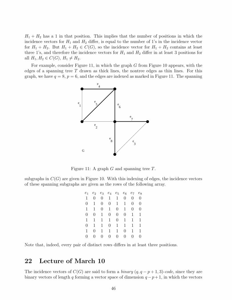
H1 + H2 has a 1 in that position. This implies that the number of positions in which theincidence vectors for H1 and H2 differ, is equal to the number of 1’s in the incidence vectorfor H1 + H2. But H1 + H2 ∈ C(G), so the incidence vector for H1 + H2 contains at leastthree 1’s, and therefore the incidence vectors for H1 and H2 differ in at least 3 positions forall H1, H2 ∈ C(G), H1 6= H2.
For example, consider Figure 11, in which the graph G from Figure 10 appears, with theedges of a spanning tree T drawn as thick lines, the nontree edges as thin lines. For thisgraph, we have q = 8, p = 6, and the edges are indexed as marked in Figure 11. The spanning
G
e
e2
1
e3
e4
e5 e
6
e7
e8
Figure 11: A graph G and spanning tree T .
subgraphs in C(G) are given in Figure 10. With this indexing of edges, the incidence vectorsof these spanning subgraphs are given as the rows of the following array.
e1 e2 e3 e4 e5 e6 e7 e81 0 0 1 1 0 0 00 1 0 0 1 1 0 01 1 0 1 0 1 0 00 0 1 0 0 0 1 11 1 1 1 0 1 1 10 1 1 0 1 1 1 11 0 1 1 1 0 1 10 0 0 0 0 0 0 0
Note that, indeed, every pair of distinct rows differs in at least three positions.
22 Lecture of March 10
The incidence vectors of C(G) are said to form a binary (q, q− p+ 1, 3)-code, since they arebinary vectors of length q forming a vector space of dimension q−p+1, in which the vectors
46

differ pairwise in at least 3 positions. If every cycle in G has length at least equal to t, thenwe get a (q, q− p+ 1, t)-code, since the vectors differ in at least t positions in this case. Theimportance of the pairwise difference in positions is that if information is encoded in termsof the vectors in the code, then errors in transmission/reception can be detected (if thereare fewer than t errors), and even corrected (if there are at most (t − 1)/2 errors). Codingtheory is studied in CO 331.
Let Nm,n, n ≥ m, denote the number of m× n {0, 1}-matrices of rank m. Then we haveN1,n = 2n−1, since a row consisting entirely of 0’s is the only way to avoid rank 1. Similarly,Nm,n = (2n − 2m−1)Nm−1,n, since the first m− 1 rows must be linearly independent (to giverank m − 1), and then row m cannot be any of the 2m−1 linear combinations of the firstm− 1 rows. We conclude that
Nm,n =m−1∏
k=0
(2n − 2k).
For example, this allows us to determine the probability that an n × n {0, 1}-matrix isnonsingular (over Z2), given by
∏n−1k=0(2
n − 2k)
2(n2)=
n∏
j=1
(1 − 2−j).
It is straightforward to determine the number of m-dimensional subspaces of a vector spaceof dimension n over Z2, since it is given by the ratio
Nm,n
Nm,m
=(2n − 1)(2n−1 − 1) · · · (2n−m+1 − 1)
(2n − 1)(2m−1 − 1) · · · (21 − 1)=
(n
m
)
2
,
where(
n
k
)q
is the Gaussian coefficient, defined near the beginning of the Lecture of February
13 (following (13)).
We now consider a spanning tree algorithm that, among other consequences, will allowus to find the shortest cycle in a graph.
Algorithm: Input a graph G, on p vertices. Initially, let subgraph D of G consist of anarbitrary vertex, denoted r, of G, with pr(r) = ∅. At every stage, find an edge {u, v} of G,with u ∈ D, and v /∈ D; add vertex v and edge {u, v} to D, with pr(v) = u. Stop whenthere is no such edge.
Claim: At termination, if D has p vertices, then it is a spanning tree of G. Otherwise, if Dhas fewer than p vertices, then G is not connected (so it has no spanning tree).
PROOF. Initially, D has no edge and a single vertex, and at every stage we add one edge andone vertex, so at stage k, D has k − 1 edges and k vertices. Also, initially D is connected,and at every stage we add an edge from a new vertex, v, to an existing vertex, u. Thus, byinduction on the number of stages, D is always connected. But a connected graph with kvertices and k − 1 edges must have a spanning tree (from Theorem 19.2), which must haveall k − 1 edges, and thus D is a tree at every stage. The first part of the claim, that D is aspanning tree of G if it has p vertices, follows immediately.
47
For the second part of the claim, suppose that D has fewer than p vertices at termination,but that G is connected. Then we have a vertex x of G, not in D. Consider a path v0. . .vn
in G, from r = v0 (where r is the initial vertex of D), to x = vn. (Such a path exists, sinceG is connected.) Now, we have v0 ∈ D, vn /∈ D, so there exists vi ∈ D, vi+1 /∈ D, for somei = 0, . . ., n − 1. But the algorithm stopped because there is no edge such as {vi, vi+1}, sowe have a contradiction, and conclude that G cannot be connected. This proves the secondpart of the claim.
23 Lecture of March 12
We call D a search tree, since the “pr” (for pointer, parent, predecessor) function allows usto find paths in D (and therefore in G): apply pr repeatedly to a vertex until we get r, toobtain a path from that vertex to the root vertex of D. If we apply pr exactly k times to dothis, then we say that the vertex is at level k in D.
For breadth first search, we apply the algorithm above, but choose an edge {u, v}, withu ∈ D, v /∈ D, for which u joined D first among all such edges. For depth first search, weapply the algorithm above, but choose an edge {u, v}, with u ∈ D, v /∈ D, for which u joinedD last among all such edges. We begin by proving the primary property of Breadth FirstSearch.
Theorem 23.1 In a Breadth First Search tree, the nontree edges join vertices that are atmost one level apart in the tree.
PROOF. We first prove that the vertices join the tree in weakly increasing order by level,using induction on the number of vertices in the tree. As base cases, the result is true ifthere are one or two vertices in the tree, since the first two vertices have levels 0 and 1,respectively. For the induction hypothesis, assume that the result holds for k vertices in thetree, for some k ≥ 2, and denote these vertices, in order of joining the tree, as v1, . . ., vk
(so the induction hypothesis is that level(v1) ≤ . . . ≤ level(vk)). Now consider the k + 1stvertex to join the tree, vk+1. Suppose pr(vk+1) = vi and pr(vk) = vj . Then we must havej ≤ i, and the induction hypothesis gives level(vj) ≤ level(vi), so we obtain
level(vk) = level(vj) + 1 ≤ level(vi) + 1 = level(vk+1),
and we have proved that the result holds for k + 1 vertices in the tree. Therefore the resultis true by mathematical induction.
Now suppose that the vertices in the Breadth First Search tree, in order of joining thetree, are v1, . . ., vm. Suppose that there is a nontree edge joining vi to vj , where i < j. Thenwe have pr(vj) = vk, where k < i, since otherwise, if k > i, we would have had pr(vj) = vi.This gives
level(vj) = level(vk) + 1 ≤ level(vi) + 1,
from the result above, and so we have proved that the nontree edge {vi, vj} joins vertices atmost one level apart.
48
One consequence of the primary property of Breadth First Search is for length of shortestpaths: The length of the shortest path between vertices u and v in a connected graph G isequal to level(v) in any Breadth First Search tree of G rooted at u. (Or, equivalently, tolevel(u) in any Breadth First Search tree of G rooted at v.) The proof is immediate, sincethere is a path of the given length, using tree edges only, and there can be no shorter path,since it would require an edge that joins vertices two or more levels apart.
Another consequence is for parity of cycles. Note that if a nontree edge joins two verticesat the same level in a Breadth First Search tree, then the fundamental cycle for that edgemust have odd length (if the vertices are at the same level, k, and the paths from thesevertices to the root first meet at a vertex at level m, then the path between these verticesin the tree has length 2(k −m), and together with the nontree edge, the fundamental cyclethus has length 2(k − m) + 1). If a nontree edge joins vertices one level apart, then thefundamental cycle for that edge must have even length (if the vertices are at levels k andk + 1, and the paths from these vertices to the root first meet at a vertex at level m, thenthe path between these vertices in the tree has length (k −m) + (k + 1 −m), and togetherwith the nontree edge, the fundamental cycle thus has length 2(k + 1 −m)).
A graph G is said to be bipartite if V (G) can be partitioned into two nonempty subsetsA,B, so that every edge of G joins a vertex of A to a vertex of B.
Theorem 23.2 A graph is bipartite if and only if it has no odd cycles.
PROOF. Consider a cycle v1, v2, . . ., vk in a bipartite graph. Then, without loss of generality,suppose v1 ∈ A (otherwise, we can interchange the sets A and B). This forces v2 ∈ B(because of edge {v1, v2}), and then we have v3 ∈ A. Continuing, we can prove by inductionthat vm ∈ A for m odd, and vm ∈ B for m even. But we also have vk ∈ B, because of edge{vk, v1}, and thus conclude that k must be even. Thus we have proved that if G is bipartite,then it has no odd cycles.
For the converse, suppose that G has no odd cycles. Then if we carry out Breadth FirstSearch on every component of G, we will never find a nontree edge joining vertices at thesame level (otherwise, we would have an odd cycle, from the discussion above, which isimpossible, from the first part of this result). But this means that the graph is bipartite,with bipartition given by A, the vertices at even levels in these trees, and B, the vertices atodd levels.
24 Lecture of March 14
Define the girth of a graph to be the length of the shortest cycle in the graph. If the graphhas no cycles, then we define its girth to be ∞. By considering Breadth First Search, we areable to prove the following result.
Theorem 24.1 For k ≥ 2, a k-regular graph of girth 5 has at least k2 + 1 vertices.
PROOF. Carry out Breadth First Search on the graph, with root vertex an arbitrary vertexv. Then the k vertices adjacent to v, call them u1, . . ., uk, all join the tree at level 1, in
49
that order. There can be no edges between ui and uj for any i 6= j, since otherwise uiujvwould be a 3-cycle in the graph, which is impossible since the girth is 5. Thus the k − 1vertices other than v that are adjacent to u1, call them w11, . . ., w1 k−1, all join the tree atlevel 2, with a pointer to u1. But u2 cannot be adjacent to any w1j , since otherwise u2w1ju1vwould be a 4-cycle, which is impossible since the girth is 5. By a similar argument, for everyi = 1, . . ., k, we establish that the k − 1 vertices other than v that are adjacent to ui, callthem wi1, . . ., wi k−1, all join the tree at level 2, with a pointer to ui. But this means thatthe tree already has 1 + k + k(k − 1) = k2 + 1 vertices, all of which are in the graph, andthe result follows.
For which values of k ≥ 2 is there a k-regular graph of girth 5 that exactly achieves thisbound of k2 + 1 vertices ? The answer is only k = 2, 3, 7 and (possibly) 57. I say “possibly”because it is still an open research problem as to whether such a graph exists – such a graphis referred to as the “Moore graph”. The proof of the impossibility of other values for k isgiven below:
Let A be the adjacency matrix for such a graph. That is, call the vertices v1, . . . , vn, insome arbitrary way, and then A is n × n, where n = k2 + 1, with (i, j)-entry equal to 1 ifvertex vi is adjacent to vertex vj . Clearly A is a symmetric 0, 1 matrix with diagonal entriesequal to 0.
Theorem 24.2 Let In be the n × n identity matrix, and Jn be the n × n matrix with allentries equal to 1. Then for n = k2 + 1 and A given above, we have
A2 = (k − 1)In + Jn −A.
PROOF. The (i, j)-entry of A2 is given by
(A2)
i,j=
n∑
m=1
Ai,mAm,j,
where Ai,j is the (i, j)-entry of A. Then, for i = j, we have
(A2)
i,i=
n∑
m=1
Ai,m = k,
for all i = 1, . . . , n, since every vertex vi has degree k. For vi adjacent to vj, we have(A2)i,j = 0, since if Ai,m = Am,j = 1 for any m, then vivjvm would be a 3-cycle in thegraph, which is a contradiction. Finally, we treat the remaining case, that i 6= j and vi isnot adjacent to vj . In this case, consider a Breadth First Search tree rooted at vi. Then vj
appears at level 2 in the tree, and pr(vj) = vℓ for some unique vℓ at level 1 in the tree, whichmeans that Ai,ℓAℓ,j = 1. But there is no other vm with Ai,mAm,j = 1, since this would implythat vivℓvjvm would be a 4-cycle in the graph, which is a contradiction. Thus, in this casewe have (A2)i,j = 1. The result follows, since the matrix on the right hand side has entriesk, 0, 1 in precisely the correct positions.
Now, let 1n be the n× 1 vector of 1’s. Then the fact that
A1n = k1n
50

follows immediately from the fact that the graph is k-regular. Thus A has 1n as an eigen-vector, with k as the corresponding eigenvalue. Now consider another eigenvector x, withcorresponding eigenvalue λ. Then the fact that A is real and symmetric implies that x and1n are orthogonal (they correspond to distinct eigenvalues). But this implies that Jnx = 0n,the n× 1 vector of 0’s. Thus from Theorem 24.2, we have
λ2x = A2x = ((k − 1)In + Jn − A)x = (k − 1)x + 0n − λx,
which implies that (λ2 + λ+ 1 − k)x = 0n, and thus that
λ2 + λ+ 1 − k = 0,
since x 6= 0n. The roots of this quadratic are −12± D
2, where D =
√4k − 3. Thus A has
eigenvalues λ0 = k, λ1 = −12+ D
2, λ2 = −1
2− D
2, and we let m0, m1, m2 be the corresponding
algebraic multiplicities. Of course, we have m0 +m1 +m2 = n. To obtain two other linearequations for m0, m1, m2, use the fact that A is real symmetric, so it is diagonalizable.Thus we have A = PΛP−1, where Λ is a diagonal matrix with diagonal entries λ0, λ1, λ2,with multiplicities m0, m1, m2, respectively. Thus we obtain Aℓ = PΛℓP−1 for any positiveinteger ℓ (prove this, say, by induction on ℓ). Now for the trace of a square matrix (thesum of diagonal entries) we have traceBC = traceCB, where B is s × t and C is t × s(for a proof, consider
∑s
i=1
∑t
j=1Bi,jCj,i =∑t
j=1
∑s
i=1Cj,iBi,j.) This gives traceAℓ = trace
ΛℓP−1P = traceΛℓ, so ℓ = 1, 2 give us the equations m0λ0 + m1λ1 + m2λ2 = trace A, andm0λ
20 + m1λ
21 + m2λ
22 = trace A2. Now, A has all diagonal entries equal to 0, so trace
A = 0, and from the proof of Theorem 24.2 above, A2 has diagonal entries all equal to k, sotraceA2 = kn. Putting these together, we have the linear system
m0 +m1 +m2 = n
λ0m0 + λ1m1 + λ2m2 = 0
λ20m0 + λ2
1m1 + λ22m2 = nk
for m0, m1, m2. But this system has determinant (λ2 − λ1)(λ2 − λ0)(λ1 − λ0) 6= 0 (called theVandermonde determinant), and so has a unique solution, given by
m0 = 1, m1 = 12k
(k +
k − 2
D
), m2 = 1
2k
(k − k − 2
D
).
(To check this, you will need the facts that λ0 = k, n = k2 + 1, λ1λ2 = 1− k, λ1 + λ2 = −1,and λ2
i = −λi + k − 1, for i = 1, 2.)The proof concludes by using the fact that m1, m2 are nonnegative integers. There are
two cases. Case 1: If 4k− 3 is not a perfect square, then D is irrational, which implies thatm1 (and m2) are irrational unless k(k − 2) = 0. But k ≥ 2, so in this case we have k = 2only. Case 2: If 4k − 3 is a perfect square, then we have k = 1
4(D2 + 3), which gives
m1 = 18(D2 + 3)
(14(D2 + 3) +
14(D2 − 5)
D
),
and when we multiply this equation by 32D and rearrange slightly, we obtain
32Dm1 −D(D2 + 3)2 −D4 + 2D2 = −15.
51
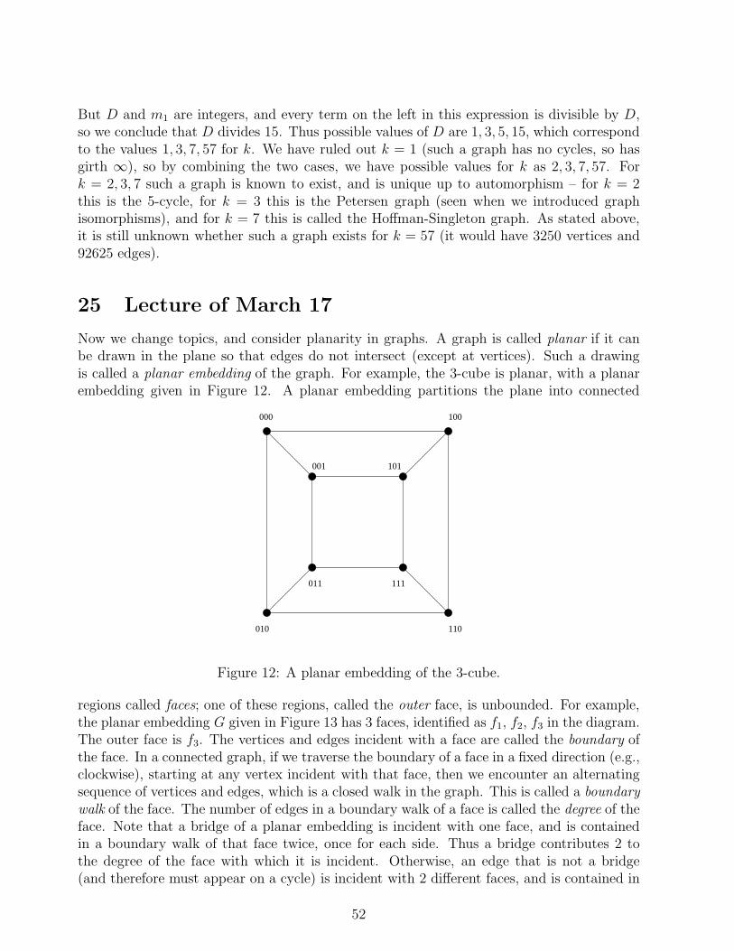
But D and m1 are integers, and every term on the left in this expression is divisible by D,so we conclude that D divides 15. Thus possible values of D are 1, 3, 5, 15, which correspondto the values 1, 3, 7, 57 for k. We have ruled out k = 1 (such a graph has no cycles, so hasgirth ∞), so by combining the two cases, we have possible values for k as 2, 3, 7, 57. Fork = 2, 3, 7 such a graph is known to exist, and is unique up to automorphism – for k = 2this is the 5-cycle, for k = 3 this is the Petersen graph (seen when we introduced graphisomorphisms), and for k = 7 this is called the Hoffman-Singleton graph. As stated above,it is still unknown whether such a graph exists for k = 57 (it would have 3250 vertices and92625 edges).
25 Lecture of March 17
Now we change topics, and consider planarity in graphs. A graph is called planar if it canbe drawn in the plane so that edges do not intersect (except at vertices). Such a drawingis called a planar embedding of the graph. For example, the 3-cube is planar, with a planarembedding given in Figure 12. A planar embedding partitions the plane into connected
000
010 110
100
001 101
011 111
Figure 12: A planar embedding of the 3-cube.
regions called faces; one of these regions, called the outer face, is unbounded. For example,the planar embedding G given in Figure 13 has 3 faces, identified as f1, f2, f3 in the diagram.The outer face is f3. The vertices and edges incident with a face are called the boundary ofthe face. In a connected graph, if we traverse the boundary of a face in a fixed direction (e.g.,clockwise), starting at any vertex incident with that face, then we encounter an alternatingsequence of vertices and edges, which is a closed walk in the graph. This is called a boundarywalk of the face. The number of edges in a boundary walk of a face is called the degree of theface. Note that a bridge of a planar embedding is incident with one face, and is containedin a boundary walk of that face twice, once for each side. Thus a bridge contributes 2 tothe degree of the face with which it is incident. Otherwise, an edge that is not a bridge(and therefore must appear on a cycle) is incident with 2 different faces, and is contained in
52
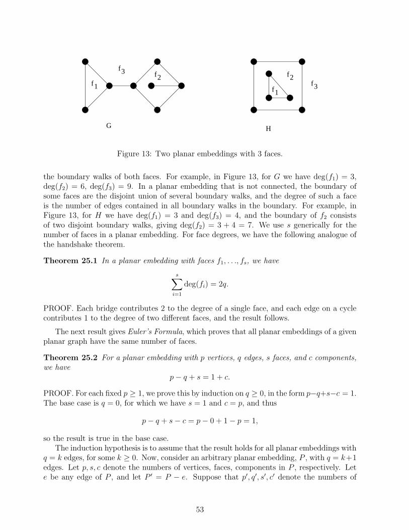
G H
f1
f2f3 f2
f1f3
Figure 13: Two planar embeddings with 3 faces.
the boundary walks of both faces. For example, in Figure 13, for G we have deg(f1) = 3,deg(f2) = 6, deg(f3) = 9. In a planar embedding that is not connected, the boundary ofsome faces are the disjoint union of several boundary walks, and the degree of such a faceis the number of edges contained in all boundary walks in the boundary. For example, inFigure 13, for H we have deg(f1) = 3 and deg(f3) = 4, and the boundary of f2 consistsof two disjoint boundary walks, giving deg(f2) = 3 + 4 = 7. We use s generically for thenumber of faces in a planar embedding. For face degrees, we have the following analogue ofthe handshake theorem.
Theorem 25.1 In a planar embedding with faces f1, . . ., fs, we have
s∑
i=1
deg(fi) = 2q.
PROOF. Each bridge contributes 2 to the degree of a single face, and each edge on a cyclecontributes 1 to the degree of two different faces, and the result follows.
The next result gives Euler’s Formula, which proves that all planar embeddings of a givenplanar graph have the same number of faces.
Theorem 25.2 For a planar embedding with p vertices, q edges, s faces, and c components,we have
p− q + s = 1 + c.
PROOF. For each fixed p ≥ 1, we prove this by induction on q ≥ 0, in the form p−q+s−c = 1.The base case is q = 0, for which we have s = 1 and c = p, and thus
p− q + s− c = p− 0 + 1 − p = 1,
so the result is true in the base case.The induction hypothesis is to assume that the result holds for all planar embeddings with
q = k edges, for some k ≥ 0. Now, consider an arbitrary planar embedding, P , with q = k+1edges. Let p, s, c denote the numbers of vertices, faces, components in P , respectively. Lete be any edge of P , and let P ′ = P − e. Suppose that p′, q′, s′, c′ denote the numbers of
53
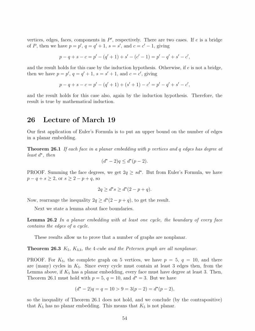
vertices, edges, faces, components in P ′, respectively. There are two cases. If e is a bridgeof P , then we have p = p′, q = q′ + 1, s = s′, and c = c′ − 1, giving
p− q + s− c = p′ − (q′ + 1) + s′ − (c′ − 1) = p′ − q′ + s′ − c′,
and the result holds for this case by the induction hypothesis. Otherwise, if e is not a bridge,then we have p = p′, q = q′ + 1, s = s′ + 1, and c = c′, giving
p− q + s− c = p′ − (q′ + 1) + (s′ + 1) − c′ = p′ − q′ + s′ − c′,
and the result holds for this case also, again by the induction hypothesis. Therefore, theresult is true by mathematical induction.
26 Lecture of March 19
Our first application of Euler’s Formula is to put an upper bound on the number of edgesin a planar embedding.
Theorem 26.1 If each face in a planar embedding with p vertices and q edges has degree atleast d⋆, then
(d⋆ − 2)q ≤ d⋆(p− 2).
PROOF. Summing the face degrees, we get 2q ≥ sd⋆. But from Euler’s Formula, we havep− q + s ≥ 2, or s ≥ 2 − p + q, so
2q ≥ d⋆s ≥ d⋆(2 − p + q).
Now, rearrange the inequality 2q ≥ d⋆(2 − p+ q), to get the result.
Next we state a lemma about face boundaries.
Lemma 26.2 In a planar embedding with at least one cycle, the boundary of every facecontains the edges of a cycle.
These results allow us to prove that a number of graphs are nonplanar.
Theorem 26.3 K5, K3,3, the 4-cube and the Petersen graph are all nonplanar.
PROOF. For K5, the complete graph on 5 vertices, we have p = 5, q = 10, and thereare (many) cycles in K5. Since every cycle must contain at least 3 edges then, from theLemma above, if K5 has a planar embedding, every face must have degree at least 3. Then,Theorem 26.1 must hold with p = 5, q = 10, and d⋆ = 3. But we have
(d⋆ − 2)q = q = 10 > 9 = 3(p− 2) = d⋆(p− 2),
so the inequality of Theorem 26.1 does not hold, and we conclude (by the contrapositive)that K5 has no planar embedding. This means that K5 is not planar.
54
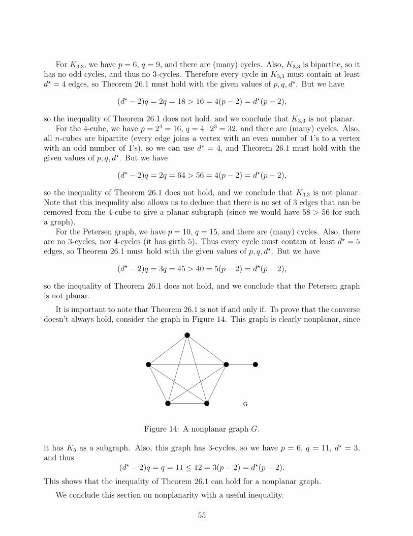
For K3,3, we have p = 6, q = 9, and there are (many) cycles. Also, K3,3 is bipartite, so ithas no odd cycles, and thus no 3-cycles. Therefore every cycle in K3,3 must contain at leastd⋆ = 4 edges, so Theorem 26.1 must hold with the given values of p, q, d⋆. But we have
(d⋆ − 2)q = 2q = 18 > 16 = 4(p− 2) = d⋆(p− 2),
so the inequality of Theorem 26.1 does not hold, and we conclude that K3,3 is not planar.For the 4-cube, we have p = 24 = 16, q = 4 · 23 = 32, and there are (many) cycles. Also,
all n-cubes are bipartite (every edge joins a vertex with an even number of 1’s to a vertexwith an odd number of 1’s), so we can use d∗ = 4, and Theorem 26.1 must hold with thegiven values of p, q, d⋆. But we have
(d⋆ − 2)q = 2q = 64 > 56 = 4(p− 2) = d⋆(p− 2),
so the inequality of Theorem 26.1 does not hold, and we conclude that K3,3 is not planar.Note that this inequality also allows us to deduce that there is no set of 3 edges that can beremoved from the 4-cube to give a planar subgraph (since we would have 58 > 56 for sucha graph).
For the Petersen graph, we have p = 10, q = 15, and there are (many) cycles. Also, thereare no 3-cycles, nor 4-cycles (it has girth 5). Thus every cycle must contain at least d⋆ = 5edges, so Theorem 26.1 must hold with the given values of p, q, d⋆. But we have
(d⋆ − 2)q = 3q = 45 > 40 = 5(p− 2) = d⋆(p− 2),
so the inequality of Theorem 26.1 does not hold, and we conclude that the Petersen graphis not planar.
It is important to note that Theorem 26.1 is not if and only if. To prove that the conversedoesn’t always hold, consider the graph in Figure 14. This graph is clearly nonplanar, since
G
Figure 14: A nonplanar graph G.
it has K5 as a subgraph. Also, this graph has 3-cycles, so we have p = 6, q = 11, d⋆ = 3,and thus
(d⋆ − 2)q = q = 11 ≤ 12 = 3(p− 2) = d⋆(p− 2).
This shows that the inequality of Theorem 26.1 can hold for a nonplanar graph.
We conclude this section on nonplanarity with a useful inequality.
55
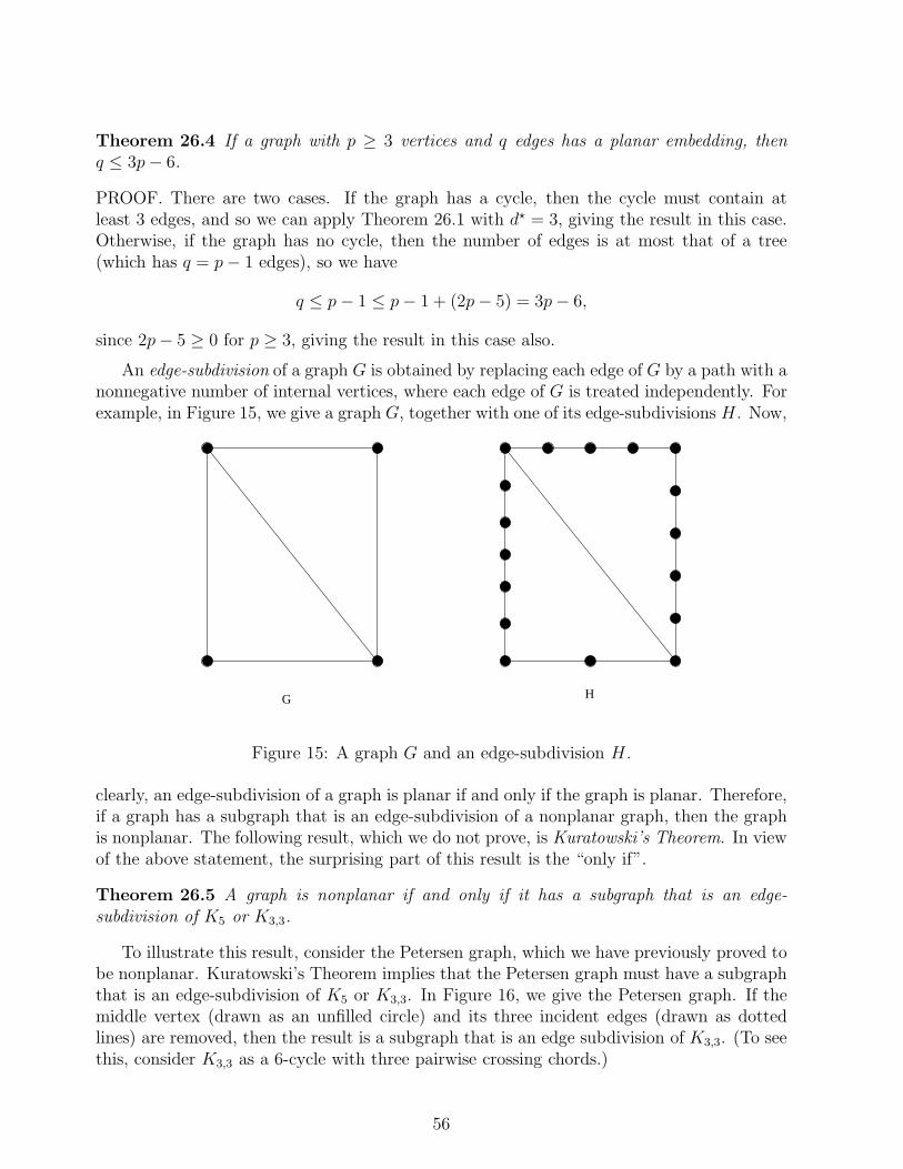
Theorem 26.4 If a graph with p ≥ 3 vertices and q edges has a planar embedding, thenq ≤ 3p− 6.
PROOF. There are two cases. If the graph has a cycle, then the cycle must contain atleast 3 edges, and so we can apply Theorem 26.1 with d⋆ = 3, giving the result in this case.Otherwise, if the graph has no cycle, then the number of edges is at most that of a tree(which has q = p− 1 edges), so we have
q ≤ p− 1 ≤ p− 1 + (2p− 5) = 3p− 6,
since 2p− 5 ≥ 0 for p ≥ 3, giving the result in this case also.
An edge-subdivision of a graph G is obtained by replacing each edge of G by a path with anonnegative number of internal vertices, where each edge of G is treated independently. Forexample, in Figure 15, we give a graph G, together with one of its edge-subdivisions H . Now,
G H
Figure 15: A graph G and an edge-subdivision H .
clearly, an edge-subdivision of a graph is planar if and only if the graph is planar. Therefore,if a graph has a subgraph that is an edge-subdivision of a nonplanar graph, then the graphis nonplanar. The following result, which we do not prove, is Kuratowski’s Theorem. In viewof the above statement, the surprising part of this result is the “only if”.
Theorem 26.5 A graph is nonplanar if and only if it has a subgraph that is an edge-subdivision of K5 or K3,3.
To illustrate this result, consider the Petersen graph, which we have previously proved tobe nonplanar. Kuratowski’s Theorem implies that the Petersen graph must have a subgraphthat is an edge-subdivision of K5 or K3,3. In Figure 16, we give the Petersen graph. If themiddle vertex (drawn as an unfilled circle) and its three incident edges (drawn as dottedlines) are removed, then the result is a subgraph that is an edge subdivision of K3,3. (To seethis, consider K3,3 as a 6-cycle with three pairwise crossing chords.)
56
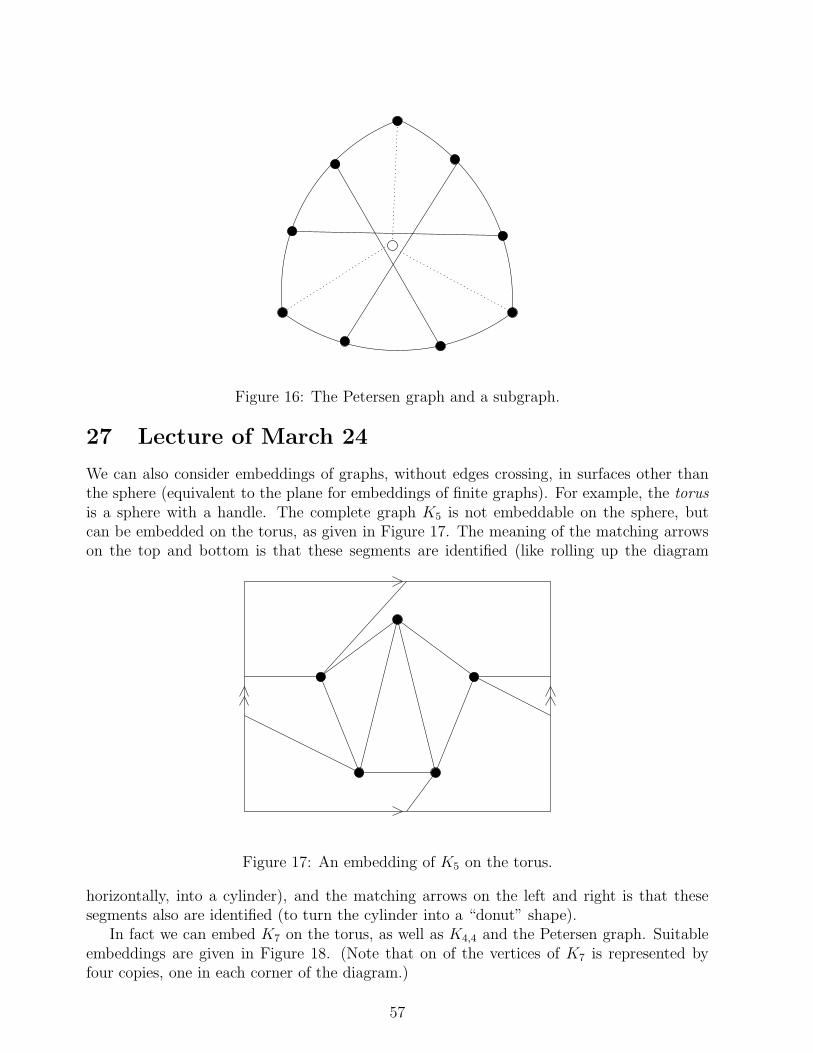
Figure 16: The Petersen graph and a subgraph.
27 Lecture of March 24
We can also consider embeddings of graphs, without edges crossing, in surfaces other thanthe sphere (equivalent to the plane for embeddings of finite graphs). For example, the torusis a sphere with a handle. The complete graph K5 is not embeddable on the sphere, butcan be embedded on the torus, as given in Figure 17. The meaning of the matching arrowson the top and bottom is that these segments are identified (like rolling up the diagram
Figure 17: An embedding of K5 on the torus.
horizontally, into a cylinder), and the matching arrows on the left and right is that thesesegments also are identified (to turn the cylinder into a “donut” shape).
In fact we can embed K7 on the torus, as well as K4,4 and the Petersen graph. Suitableembeddings are given in Figure 18. (Note that on of the vertices of K7 is represented byfour copies, one in each corner of the diagram.)
57
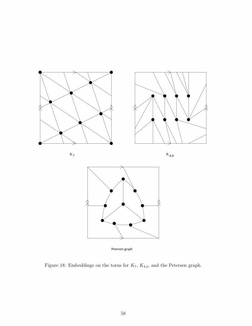
K7 K4,4
Petersen graph
Figure 18: Embeddings on the torus for K7, K4,4, and the Petersen graph.
58
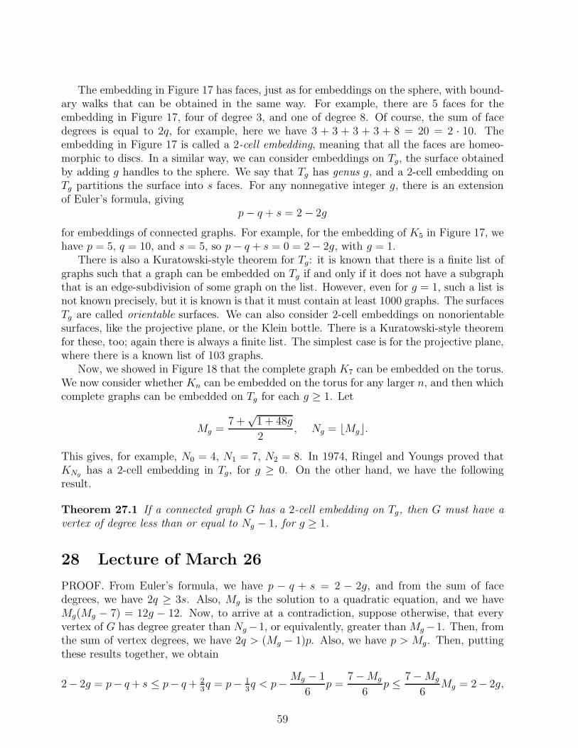
The embedding in Figure 17 has faces, just as for embeddings on the sphere, with bound-ary walks that can be obtained in the same way. For example, there are 5 faces for theembedding in Figure 17, four of degree 3, and one of degree 8. Of course, the sum of facedegrees is equal to 2q, for example, here we have 3 + 3 + 3 + 3 + 8 = 20 = 2 · 10. Theembedding in Figure 17 is called a 2-cell embedding, meaning that all the faces are homeo-morphic to discs. In a similar way, we can consider embeddings on Tg, the surface obtainedby adding g handles to the sphere. We say that Tg has genus g, and a 2-cell embedding onTg partitions the surface into s faces. For any nonnegative integer g, there is an extensionof Euler’s formula, giving
p− q + s = 2 − 2g
for embeddings of connected graphs. For example, for the embedding of K5 in Figure 17, wehave p = 5, q = 10, and s = 5, so p− q + s = 0 = 2 − 2g, with g = 1.
There is also a Kuratowski-style theorem for Tg: it is known that there is a finite list ofgraphs such that a graph can be embedded on Tg if and only if it does not have a subgraphthat is an edge-subdivision of some graph on the list. However, even for g = 1, such a list isnot known precisely, but it is known is that it must contain at least 1000 graphs. The surfacesTg are called orientable surfaces. We can also consider 2-cell embeddings on nonorientablesurfaces, like the projective plane, or the Klein bottle. There is a Kuratowski-style theoremfor these, too; again there is always a finite list. The simplest case is for the projective plane,where there is a known list of 103 graphs.
Now, we showed in Figure 18 that the complete graph K7 can be embedded on the torus.We now consider whether Kn can be embedded on the torus for any larger n, and then whichcomplete graphs can be embedded on Tg for each g ≥ 1. Let
Mg =7 +
√1 + 48g
2, Ng = ⌊Mg⌋.
This gives, for example, N0 = 4, N1 = 7, N2 = 8. In 1974, Ringel and Youngs proved thatKNg
has a 2-cell embedding in Tg, for g ≥ 0. On the other hand, we have the followingresult.
Theorem 27.1 If a connected graph G has a 2-cell embedding on Tg, then G must have avertex of degree less than or equal to Ng − 1, for g ≥ 1.
28 Lecture of March 26
PROOF. From Euler’s formula, we have p − q + s = 2 − 2g, and from the sum of facedegrees, we have 2q ≥ 3s. Also, Mg is the solution to a quadratic equation, and we haveMg(Mg − 7) = 12g − 12. Now, to arrive at a contradiction, suppose otherwise, that everyvertex of G has degree greater than Ng −1, or equivalently, greater than Mg −1. Then, fromthe sum of vertex degrees, we have 2q > (Mg − 1)p. Also, we have p > Mg. Then, puttingthese results together, we obtain
2− 2g = p− q+ s ≤ p− q+ 23q = p− 1
3q < p−Mg − 1
6p =
7 −Mg
6p ≤ 7 −Mg
6Mg = 2− 2g,
59
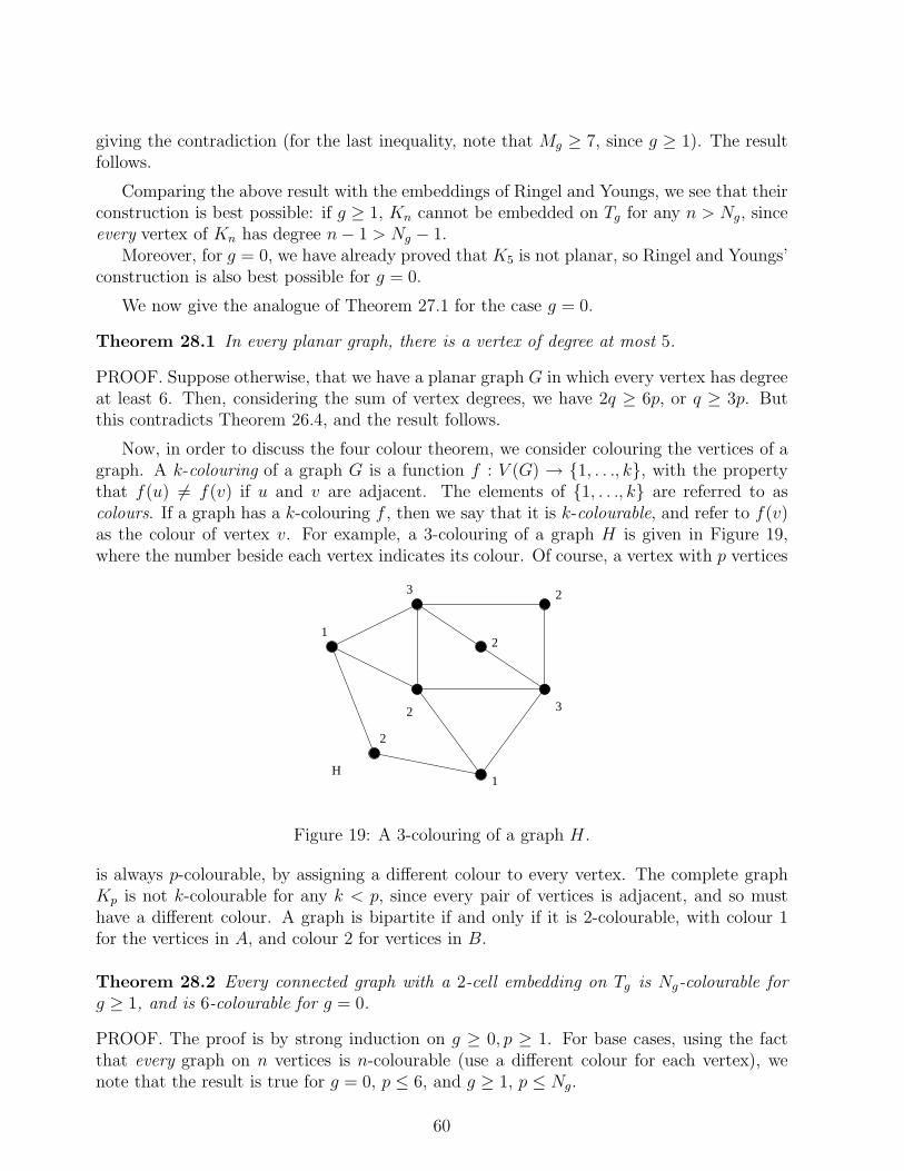
giving the contradiction (for the last inequality, note that Mg ≥ 7, since g ≥ 1). The resultfollows.
Comparing the above result with the embeddings of Ringel and Youngs, we see that theirconstruction is best possible: if g ≥ 1, Kn cannot be embedded on Tg for any n > Ng, sinceevery vertex of Kn has degree n− 1 > Ng − 1.
Moreover, for g = 0, we have already proved that K5 is not planar, so Ringel and Youngs’construction is also best possible for g = 0.
We now give the analogue of Theorem 27.1 for the case g = 0.
Theorem 28.1 In every planar graph, there is a vertex of degree at most 5.
PROOF. Suppose otherwise, that we have a planar graph G in which every vertex has degreeat least 6. Then, considering the sum of vertex degrees, we have 2q ≥ 6p, or q ≥ 3p. Butthis contradicts Theorem 26.4, and the result follows.
Now, in order to discuss the four colour theorem, we consider colouring the vertices of agraph. A k-colouring of a graph G is a function f : V (G) → {1, . . ., k}, with the propertythat f(u) 6= f(v) if u and v are adjacent. The elements of {1, . . ., k} are referred to ascolours. If a graph has a k-colouring f , then we say that it is k-colourable, and refer to f(v)as the colour of vertex v. For example, a 3-colouring of a graph H is given in Figure 19,where the number beside each vertex indicates its colour. Of course, a vertex with p vertices
H
1
3
2
2
1
3
2
2
Figure 19: A 3-colouring of a graph H .
is always p-colourable, by assigning a different colour to every vertex. The complete graphKp is not k-colourable for any k < p, since every pair of vertices is adjacent, and so musthave a different colour. A graph is bipartite if and only if it is 2-colourable, with colour 1for the vertices in A, and colour 2 for vertices in B.
Theorem 28.2 Every connected graph with a 2-cell embedding on Tg is Ng-colourable forg ≥ 1, and is 6-colourable for g = 0.
PROOF. The proof is by strong induction on g ≥ 0, p ≥ 1. For base cases, using the factthat every graph on n vertices is n-colourable (use a different colour for each vertex), wenote that the result is true for g = 0, p ≤ 6, and g ≥ 1, p ≤ Ng.
60
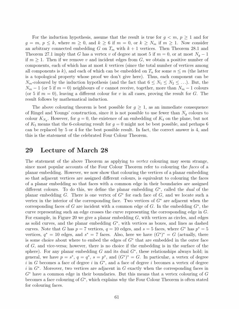
For the induction hypothesis, assume that the result is true for g < m, p ≥ 1 and forg = m, p ≤ k, where m ≥ 0, and k ≥ 6 if m = 0, or k ≥ Nm if m ≥ 1. Now consideran arbitrary connected embedding G on Tm with k + 1 vertices. Then Theorem 28.1 andTheorem 27.1 imply that G has a vertex v of degree at most 5 if m = 0, or at most Ng − 1if m ≥ 1. Then if we remove v and incident edges from G, we obtain a positive number ofcomponents, each of which has at most k vertices (since the total number of vertices amongall components is k), and each of which can be embedded on Tn for some n ≤ m (the latteris a topological property whose proof we don’t give here). Thus, each component can beNm-coloured by the induction hypothesis (and the fact that 6 ≤ N1 ≤ N2 ≤ . . .). But, theNm − 1 (or 5 if m = 0) neighbours of v cannot receive, together, more than Nm − 1 colours(or 5 if m = 0), leaving a different colour for v in all cases, proving the result for G. Theresult follows by mathematical induction.
The above colouring theorem is best possible for g ≥ 1, as an immediate consequenceof Ringel and Youngs’ construction, since it is not possible to use fewer than Ng colours tocolour KNg
. However, for g = 0, the existence of an embedding of K4 on the plane, but notof K5 means that the 6-colouring result for g = 0 might not be best possible, and perhaps 6can be replaced by 5 or 4 for the best possible result. In fact, the correct answer is 4, andthis is the statement of the celebrated Four Colour Theorem.
29 Lecture of March 28
The statement of the above Theorem as applying to vertex colouring may seem strange,since most popular accounts of the Four Colour Theorem refer to colouring the faces of aplanar embedding. However, we now show that colouring the vertices of a planar embeddingso that adjacent vertices are assigned different colours, is equivalent to colouring the facesof a planar embedding so that faces with a common edge in their boundaries are assigneddifferent colours. To do this, we define the planar embedding G∗, called the dual of theplanar embedding G. There is one vertex of G∗ for each face of G, and we locate such avertex in the interior of the corresponding face. Two vertices of G∗ are adjacent when thecorresponding faces of G are incident with a common edge of G. In the embedding G∗, thecurve representing such an edge crosses the curve representing the corresponding edge in G.For example, in Figure 20 we give a planar embedding G, with vertices as circles, and edgesas solid curves, and the planar embedding G∗, with vertices as boxes, and lines as dashedcurves. Note that G has p = 7 vertices, q = 10 edges, and s = 5 faces, where G∗ has p∗ = 5vertices, q∗ = 10 edges, and s∗ = 7 faces. Also, here we have (G∗)∗ = G (actually, thereis some choice about where to embed the edges of G∗ that are embedded in the outer faceof G, and vice-versa; however, there is no choice if the embedding is in the surface of thesphere). For any planar embedding G and its dual G∗, these relationships always hold; ingeneral, we have p = s∗, q = q∗, s = p∗, and (G∗)∗ = G. In particular, a vertex of degreei in G becomes a face of degree i in G∗, and a face of degree i becomes a vertex of degreei in G∗. Moreover, two vertices are adjacent in G exactly when the corresponding faces inG∗ have a common edge in their boundaries. But this means that a vertex colouring of Gbecomes a face colouring of G∗, which explains why the Four Colour Theorem is often statedfor colouring faces.
61
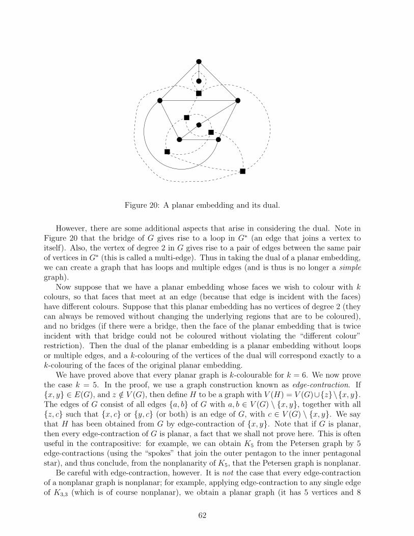
Figure 20: A planar embedding and its dual.
However, there are some additional aspects that arise in considering the dual. Note inFigure 20 that the bridge of G gives rise to a loop in G∗ (an edge that joins a vertex toitself). Also, the vertex of degree 2 in G gives rise to a pair of edges between the same pairof vertices in G∗ (this is called a multi-edge). Thus in taking the dual of a planar embedding,we can create a graph that has loops and multiple edges (and is thus is no longer a simplegraph).
Now suppose that we have a planar embedding whose faces we wish to colour with kcolours, so that faces that meet at an edge (because that edge is incident with the faces)have different colours. Suppose that this planar embedding has no vertices of degree 2 (theycan always be removed without changing the underlying regions that are to be coloured),and no bridges (if there were a bridge, then the face of the planar embedding that is twiceincident with that bridge could not be coloured without violating the “different colour”restriction). Then the dual of the planar embedding is a planar embedding without loopsor multiple edges, and a k-colouring of the vertices of the dual will correspond exactly to ak-colouring of the faces of the original planar embedding.
We have proved above that every planar graph is k-colourable for k = 6. We now provethe case k = 5. In the proof, we use a graph construction known as edge-contraction. If{x, y} ∈ E(G), and z /∈ V (G), then define H to be a graph with V (H) = V (G)∪{z}\{x, y}.The edges of G consist of all edges {a, b} of G with a, b ∈ V (G) \ {x, y}, together with all{z, c} such that {x, c} or {y, c} (or both) is an edge of G, with c ∈ V (G) \ {x, y}. We saythat H has been obtained from G by edge-contraction of {x, y}. Note that if G is planar,then every edge-contraction of G is planar, a fact that we shall not prove here. This is oftenuseful in the contrapositive: for example, we can obtain K5 from the Petersen graph by 5edge-contractions (using the “spokes” that join the outer pentagon to the inner pentagonalstar), and thus conclude, from the nonplanarity of K5, that the Petersen graph is nonplanar.
Be careful with edge-contraction, however. It is not the case that every edge-contractionof a nonplanar graph is nonplanar; for example, applying edge-contraction to any single edgeof K3,3 (which is of course nonplanar), we obtain a planar graph (it has 5 vertices and 8
62
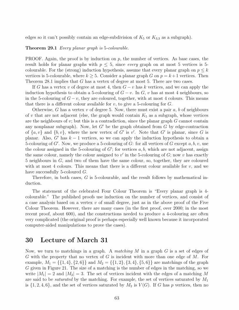
edges so it can’t possibly contain an edge-subdivision of K5 or K3,3 as a subgraph).
Theorem 29.1 Every planar graph is 5-colourable.
PROOF. Again, the proof is by induction on p, the number of vertices. As base cases, theresult holds for planar graphs with p ≤ 5, since every graph on at most 5 vertices is 5-colourable. For the (strong) induction hypothesis, assume that every planar graph on p ≤ kvertices is 5-colourable, where k ≥ 5. Consider a planar graph G on p = k+1 vertices. ThenTheorem 28.1 implies that G has a vertex of degree at most 5. There are two cases.
If G has a vertex v of degree at most 4, then G− v has k vertices, and we can apply theinduction hypothesis to obtain a 5-colouring of G− v. In G, v has at most 4 neighbours, soin the 5-colouring of G− v, they are coloured, together, with at most 4 colours. This meansthat there is a different colour available for v, to give a 5-colouring for G.
Otherwise, G has a vertex v of degree 5. Now, there must exist a pair a, b of neighboursof v that are not adjacent (else, the graph would contain K5 as a subgraph, whose verticesare the neighbours of v; but this is a contradiction, since the planar graph G cannot containany nonplanar subgraph). Now, let G′ be the graph obtained from G by edge-contractionof {a, v} and {b, v}, where the new vertex of G′ is v′. Note that G′ is planar, since G isplanar. Also, G′ has k − 1 vertices, so we can apply the induction hypothesis to obtain a5-colouring of G′. Now, we produce a 5-colouring of G: for all vertices of G except a, b, v, usethe colour assigned in the 5-colouring of G′; for vertices a, b, which are not adjacent, assignthe same colour, namely the colour assigned to v′ in the 5-colouring of G; now v has exactly5 neighbours in G, and two of them have the same colour, so, together, they are colouredwith at most 4 colours. This means that there is a different colour available for v, and wehave successfully 5-coloured G.
Therefore, in both cases, G is 5-colourable, and the result follows by mathematical in-duction.
The statement of the celebrated Four Colour Theorem is “Every planar graph is 4-colourable.” The published proofs use induction on the number of vertices, and consist ofa case analysis based on a vertex v of small degree, just as in the above proof of the FiveColour Theorem. However, there are many cases (in the first proof, over 2000; in the mostrecent proof, about 600), and the constructions needed to produce a 4-colouring are oftenvery complicated (the original proof is perhaps especially well known because it incorporatedcomputer-aided manipulations to prove the cases).
30 Lecture of March 31
Now, we turn to matchings in a graph. A matching M in a graph G is a set of edges ofG with the property that no vertex of G is incident with more than one edge of M . Forexample, M1 = {{1, 4}, {2, 6}} and M2 = {{1, 2}, {3, 4}, {5, 6}} are matchings of the graphG given in Figure 21. The size of a matching is the number of edges in the matching, so wewrite |M1| = 2 and |M2| = 3. The set of vertices incident with the edges of a matching Mare said to be saturated by the matching. For example, the set of vertices saturated by M1
is {1, 2, 4, 6}, and the set of vertices saturated by M2 is V (G). If G has p vertices, then no
63
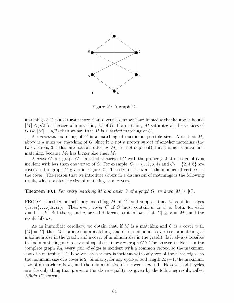
1
2
3
4
5
6
G
Figure 21: A graph G.
matching of G can saturate more than p vertices, so we have immediately the upper bound|M | ≤ p/2 for the size of a matching M of G. If a matching M saturates all the vertices ofG (so |M | = p/2) then we say that M is a perfect matching of G.
A maximum matching of G is a matching of maximum possible size. Note that M1
above is a maximal matching of G, since it is not a proper subset of another matching (thetwo vertices, 3, 5 that are not saturated by M1 are not adjacent), but it is not a maximummatching, because M2 has bigger size than M1.
A cover C in a graph G is a set of vertices of G with the property that no edge of G isincident with less than one vertex of C. For example, C1 = {1, 2, 3, 4} and C2 = {2, 4, 6} arecovers of the graph G given in Figure 21. The size of a cover is the number of vertices inthe cover. The reason that we introduce covers in a discussion of matchings is the followingresult, which relates the size of matchings and covers.
Theorem 30.1 For every matching M and cover C of a graph G, we have |M | ≤ |C|.
PROOF. Consider an arbitrary matching M of G, and suppose that M contains edges{u1, v1}, . . .{uk, vk}. Then every cover C of G must contain ui or vi or both, for eachi = 1, . . ., k. But the ui and vi are all different, so it follows that |C| ≥ k = |M |, and theresult follows.
As an immediate corollary, we obtain that, if M is a matching and C is a cover with|M | = |C|, then M is a maximum matching, and C is a minimum cover (i.e., a matching ofmaximum size in the graph, and a cover of minimum size in the graph). Is it always possibleto find a matching and a cover of equal size in every graph G ? The answer is “No” – in thecomplete graph K3, every pair of edges is incident with a common vertex, so the maximumsize of a matching is 1; however, each vertex is incident with only two of the three edges, sothe minimum size of a cover is 2. Similarly, for any cycle of odd length 2m+1, the maximumsize of a matching is m, and the minimum size of a cover is m + 1. However, odd cyclesare the only thing that prevents the above equality, as given by the following result, calledKonig’s Theorem.
64
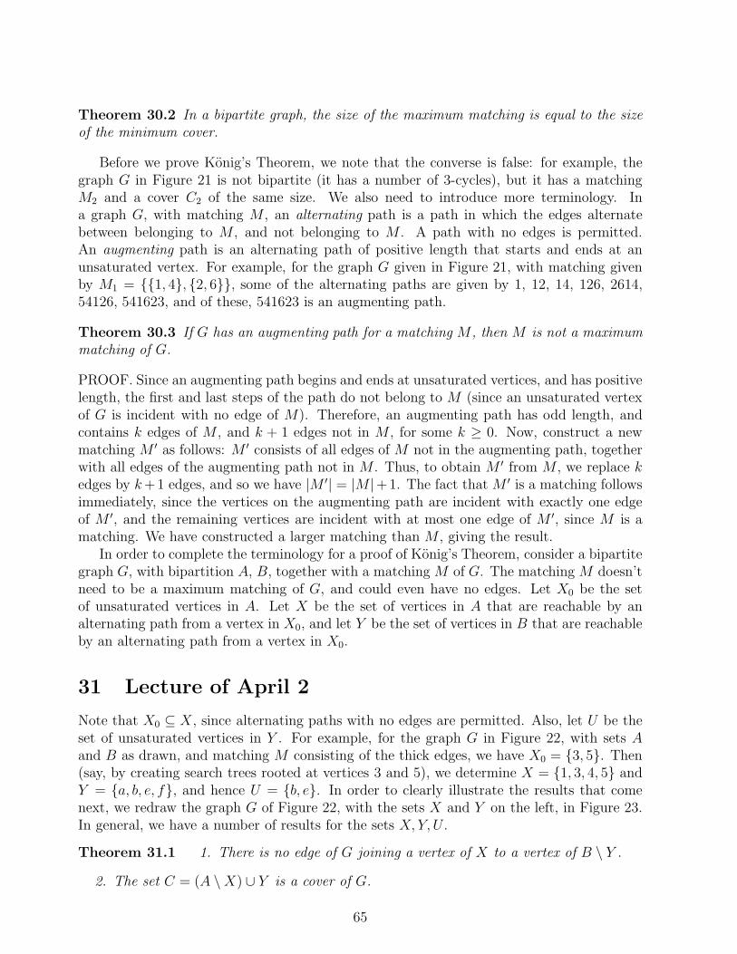
Theorem 30.2 In a bipartite graph, the size of the maximum matching is equal to the sizeof the minimum cover.
Before we prove Konig’s Theorem, we note that the converse is false: for example, thegraph G in Figure 21 is not bipartite (it has a number of 3-cycles), but it has a matchingM2 and a cover C2 of the same size. We also need to introduce more terminology. Ina graph G, with matching M , an alternating path is a path in which the edges alternatebetween belonging to M , and not belonging to M . A path with no edges is permitted.An augmenting path is an alternating path of positive length that starts and ends at anunsaturated vertex. For example, for the graph G given in Figure 21, with matching givenby M1 = {{1, 4}, {2, 6}}, some of the alternating paths are given by 1, 12, 14, 126, 2614,54126, 541623, and of these, 541623 is an augmenting path.
Theorem 30.3 If G has an augmenting path for a matching M , then M is not a maximummatching of G.
PROOF. Since an augmenting path begins and ends at unsaturated vertices, and has positivelength, the first and last steps of the path do not belong to M (since an unsaturated vertexof G is incident with no edge of M). Therefore, an augmenting path has odd length, andcontains k edges of M , and k + 1 edges not in M , for some k ≥ 0. Now, construct a newmatching M ′ as follows: M ′ consists of all edges of M not in the augmenting path, togetherwith all edges of the augmenting path not in M . Thus, to obtain M ′ from M , we replace kedges by k+1 edges, and so we have |M ′| = |M |+1. The fact that M ′ is a matching followsimmediately, since the vertices on the augmenting path are incident with exactly one edgeof M ′, and the remaining vertices are incident with at most one edge of M ′, since M is amatching. We have constructed a larger matching than M , giving the result.
In order to complete the terminology for a proof of Konig’s Theorem, consider a bipartitegraph G, with bipartition A, B, together with a matching M of G. The matching M doesn’tneed to be a maximum matching of G, and could even have no edges. Let X0 be the setof unsaturated vertices in A. Let X be the set of vertices in A that are reachable by analternating path from a vertex in X0, and let Y be the set of vertices in B that are reachableby an alternating path from a vertex in X0.
31 Lecture of April 2
Note that X0 ⊆ X, since alternating paths with no edges are permitted. Also, let U be theset of unsaturated vertices in Y . For example, for the graph G in Figure 22, with sets Aand B as drawn, and matching M consisting of the thick edges, we have X0 = {3, 5}. Then(say, by creating search trees rooted at vertices 3 and 5), we determine X = {1, 3, 4, 5} andY = {a, b, e, f}, and hence U = {b, e}. In order to clearly illustrate the results that comenext, we redraw the graph G of Figure 22, with the sets X and Y on the left, in Figure 23.In general, we have a number of results for the sets X, Y, U .
Theorem 31.1 1. There is no edge of G joining a vertex of X to a vertex of B \ Y .
2. The set C = (A \X) ∪ Y is a cover of G.
65
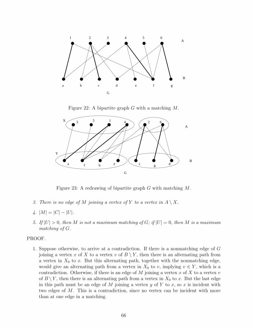
1 2 3 4 5 6
a b c d e f g
A
B
G
Figure 22: A bipartite graph G with a matching M .
5 1 4 2 6
f b e
G
3
a c dg
X
Y
A
B
Figure 23: A redrawing of bipartite graph G with matching M .
3. There is no edge of M joining a vertex of Y to a vertex in A \X.
4. |M | = |C| − |U |.
5. If |U | > 0, then M is not a maximum matching of G; if |U | = 0, then M is a maximummatching of G.
PROOF.
1. Suppose otherwise, to arrive at a contradiction. If there is a nonmatching edge of Gjoining a vertex x of X to a vertex v of B \ Y , then there is an alternating path froma vertex in X0 to x. But this alternating path, together with the nonmatching edge,would give an alternating path from a vertex in X0 to v, implying v ∈ Y , which is acontradiction. Otherwise, if there is an edge of M joining a vertex x of X to a vertex vof B \ Y , then there is an alternating path from a vertex in X0 to x. But the last edgein this path must be an edge of M joining a vertex y of Y to x, so x is incident withtwo edges of M . This is a contradiction, since no vertex can be incident with morethan at one edge in a matching.
66
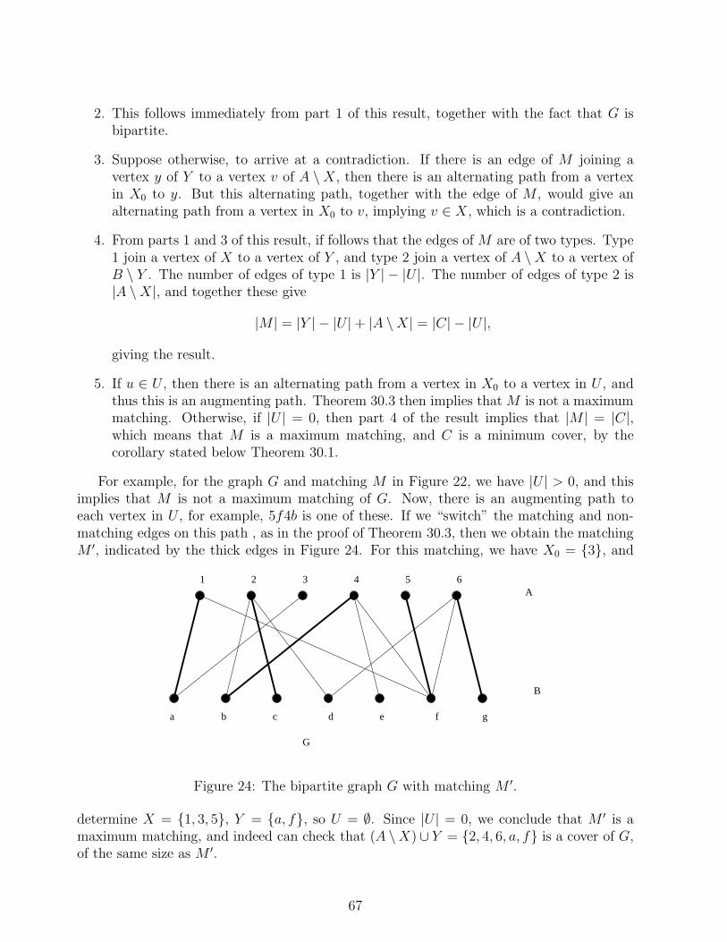
2. This follows immediately from part 1 of this result, together with the fact that G isbipartite.
3. Suppose otherwise, to arrive at a contradiction. If there is an edge of M joining avertex y of Y to a vertex v of A \X, then there is an alternating path from a vertexin X0 to y. But this alternating path, together with the edge of M , would give analternating path from a vertex in X0 to v, implying v ∈ X, which is a contradiction.
4. From parts 1 and 3 of this result, if follows that the edges of M are of two types. Type1 join a vertex of X to a vertex of Y , and type 2 join a vertex of A \X to a vertex ofB \ Y . The number of edges of type 1 is |Y | − |U |. The number of edges of type 2 is|A \X|, and together these give
|M | = |Y | − |U | + |A \X| = |C| − |U |,
giving the result.
5. If u ∈ U , then there is an alternating path from a vertex in X0 to a vertex in U , andthus this is an augmenting path. Theorem 30.3 then implies that M is not a maximummatching. Otherwise, if |U | = 0, then part 4 of the result implies that |M | = |C|,which means that M is a maximum matching, and C is a minimum cover, by thecorollary stated below Theorem 30.1.
For example, for the graph G and matching M in Figure 22, we have |U | > 0, and thisimplies that M is not a maximum matching of G. Now, there is an augmenting path toeach vertex in U , for example, 5f4b is one of these. If we “switch” the matching and non-matching edges on this path , as in the proof of Theorem 30.3, then we obtain the matchingM ′, indicated by the thick edges in Figure 24. For this matching, we have X0 = {3}, and
1 2 3 4 5 6
a b c d e f g
G
A
B
Figure 24: The bipartite graph G with matching M ′.
determine X = {1, 3, 5}, Y = {a, f}, so U = ∅. Since |U | = 0, we conclude that M ′ is amaximum matching, and indeed can check that (A \X) ∪ Y = {2, 4, 6, a, f} is a cover of G,of the same size as M ′.
67
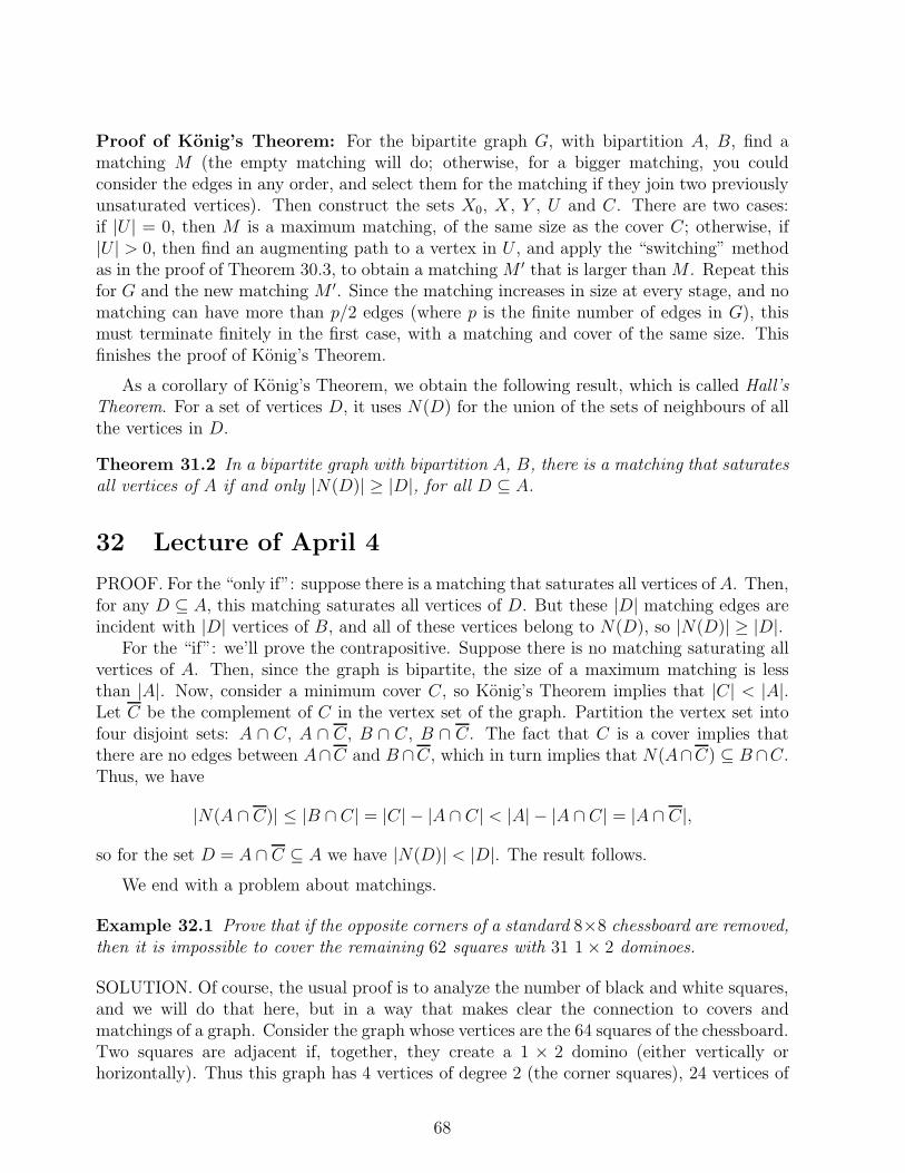
Proof of Konig’s Theorem: For the bipartite graph G, with bipartition A, B, find amatching M (the empty matching will do; otherwise, for a bigger matching, you couldconsider the edges in any order, and select them for the matching if they join two previouslyunsaturated vertices). Then construct the sets X0, X, Y , U and C. There are two cases:if |U | = 0, then M is a maximum matching, of the same size as the cover C; otherwise, if|U | > 0, then find an augmenting path to a vertex in U , and apply the “switching” methodas in the proof of Theorem 30.3, to obtain a matching M ′ that is larger than M . Repeat thisfor G and the new matching M ′. Since the matching increases in size at every stage, and nomatching can have more than p/2 edges (where p is the finite number of edges in G), thismust terminate finitely in the first case, with a matching and cover of the same size. Thisfinishes the proof of Konig’s Theorem.
As a corollary of Konig’s Theorem, we obtain the following result, which is called Hall’sTheorem. For a set of vertices D, it uses N(D) for the union of the sets of neighbours of allthe vertices in D.
Theorem 31.2 In a bipartite graph with bipartition A, B, there is a matching that saturatesall vertices of A if and only |N(D)| ≥ |D|, for all D ⊆ A.
32 Lecture of April 4
PROOF. For the “only if”: suppose there is a matching that saturates all vertices of A. Then,for any D ⊆ A, this matching saturates all vertices of D. But these |D| matching edges areincident with |D| vertices of B, and all of these vertices belong to N(D), so |N(D)| ≥ |D|.
For the “if”: we’ll prove the contrapositive. Suppose there is no matching saturating allvertices of A. Then, since the graph is bipartite, the size of a maximum matching is lessthan |A|. Now, consider a minimum cover C, so Konig’s Theorem implies that |C| < |A|.Let C be the complement of C in the vertex set of the graph. Partition the vertex set intofour disjoint sets: A ∩ C, A ∩ C, B ∩ C, B ∩ C. The fact that C is a cover implies thatthere are no edges between A∩C and B ∩C, which in turn implies that N(A∩C) ⊆ B∩C.Thus, we have
|N(A ∩ C)| ≤ |B ∩ C| = |C| − |A ∩ C| < |A| − |A ∩ C| = |A ∩ C|,
so for the set D = A ∩ C ⊆ A we have |N(D)| < |D|. The result follows.
We end with a problem about matchings.
Example 32.1 Prove that if the opposite corners of a standard 8×8 chessboard are removed,then it is impossible to cover the remaining 62 squares with 31 1 × 2 dominoes.
SOLUTION. Of course, the usual proof is to analyze the number of black and white squares,and we will do that here, but in a way that makes clear the connection to covers andmatchings of a graph. Consider the graph whose vertices are the 64 squares of the chessboard.Two squares are adjacent if, together, they create a 1 × 2 domino (either vertically orhorizontally). Thus this graph has 4 vertices of degree 2 (the corner squares), 24 vertices of
68

degree 3 (the squares on the outside, not on the corners), and 36 squares of degree 4 (thesquares on the inside of the board). A covering of the chessboard with 1 × 2 dominoes isa perfect matching of the graph. Note that the graph is bipartite (with the sets A and Bgiven by the 32 black and 32 white squares, respectively).
When the opposite corners are removed, this problem asks us to find a perfect matchingof the graph with two vertices in the same class removed, so we must find a perfect matchingof a bipartite graph whose bipartite classes have 30 and 32 vertices. But the 30 vertices inone class give a cover of the graph of size 30, and so Theorem 30.1 implies that no matchinghas size greater than 30. Thus it is impossible to find a perfect matching (of size 62/2 = 31).
69