enumerative combinatorics related to partition shapes - diva portal

Enumerative combinatorics related to partition shapes

JONAS SJOSTRAND

Doctoral ThesisStockholm, Sweden 2007

TRITA-MAT-07-MA-01ISSN 1401-2278ISRN KTH/MAT/DA 07/01-SEISBN 978-91-7178-588-6

Kungl. Tekniska HogskolanInstitutionen for matematik

SE-100 44 StockholmSWEDEN

Akademisk avhandling som med tillstand av Kungl. Tekniska Hogskolan framlaggstill offentlig granskning for avlaggande av teknologie doktorsexamen i matematikfredagen den 23 mars kl. 13.15 i sal F3, KTH, Lindstedtsvagen 26, Stockholm.

c© Jonas Sjostrand, februari 2007

Tryck: Universitetsservice US-AB

Abstract

This thesis deals with enumerative combinatorics applied to three different objects relatedto partition shapes, namely tableaux, restricted words, and Bruhat intervals. The mainscientific contributions are the following.

Paper I: Let the sign of a standard Young tableau be the sign of the permutation youget by reading it row by row from left to right, like a book. A conjecture by RichardStanley says that the sum of the signs of all SYTs with n squares is 2⌊n/2⌋. We provea generalisation of this conjecture using the Robinson-Schensted correspondence anda new concept called chess tableaux. The proof is built on a remarkably simplerelation between the sign of a permutation π and the signs of its RS-correspondingtableaux P and Q, namely sgn π = (−1)v sgn P sgn Q, where v is the number ofdisjoint vertical dominoes that fit in the partition shape of P and Q.

The sign-imbalance of a partition shape is defined as the sum of the signs of all stand-ard Young tableaux of that shape. As a further application of the sign-transferringformula above, we also prove a sharpening of another conjecture by Stanley concern-ing weighted sums of squares of sign-imbalances.

Paper II: We generalise some of the results in paper I to skew tableaux. More precisely,we examine how the sign property is transferred by the skew Robinson-Schenstedcorrespondence invented by Sagan and Stanley. The result is a surprisingly simplegeneralisation of the ordinary non-skew formula above.

As an application, we find vanishing weighted sums of squares of sign-imbalances,thereby generalising a variant of Stanley’s second conjecture.

Paper III: The following special case of a conjecture by Loehr and Warrington wasproved by Ekhad, Vatter, and Zeilberger:

There are 10n zero-sum words of length 5n in the alphabet {+3,−2} such that noconsecutive subword begins with +3, ends with −2, and sums to −2.

We give a simple bijective proof of the conjecture in its original and more generalsetting where 3 and 2 are replaced by any relatively prime positive integers a and b,10n is replaced by

`

a+ba

´n, and 5n is replaced by (a + b)n. To do this we reformulate

the problem in terms of cylindrical lattice walks which can be interpreted as thesouth-east border of certain partition shapes.

Paper IV: We characterise the permutations π such that the elements in the closedlower Bruhat interval [id, π] of the symmetric group correspond to non-capturingrook configurations on a skew Ferrers board. These intervals turn out to be exactlythose whose flag manifolds are defined by inclusions, as defined by Gasharov andReiner.

The characterisation connects Poincare polynomials (rank-generating functions) ofBruhat intervals with q-rook polynomials, and we are able to compute the Poincarepolynomial of some particularly interesting intervals in the finite Weyl groups An

and Bn. The expressions involve q-Stirling numbers of the second kind, and for thegroup An putting q = 1 yields the poly-Bernoulli numbers defined by Kaneko.

Keywords: partition shape, sign-imbalance, Robinson-Schensted correspondence, chesstableau; restricted word, cylindrical lattice walk; Poincare polynomial, Bruhat interval,rook polynomial, pattern avoidance.

Sammanfattning

Amnet for denna avhandling ar enumerativ kombinatorik tillampad pa tre olika objekt medanknytning till partitionsformer, namligen tablaer, begransade ord och bruhatintervall.Dom viktigaste vetenskapliga bidragen ar foljande.

Artikel I: Lat tecknet av en standardtabla vara tecknet hos permutationen man farom man laser tablan rad for rad fran vanster till hoger, som en bok. En for-modan av Richard Stanley sajer att teckensumman av alla standardtablaer medn rutor ar 2⌊n/2⌋. Vi visar en generalisering av denna formodan med hjalp avRobinson-Schensted-korrespondensen och ett nytt begrepp som vi kallar schack-tablaer. Beviset bygger pa ett anmarkningsvart enkelt samband mellan tecknet hosen permutation π och tecknen hos dess RS-motsvarande tablaer P och Q, namligensgn π = (−1)v sgn P sgn Q, dar v ar antalet disjunkta vertikala dominobrickor somfar plats i partitionsformen hos P och Q.

Teckenobalansen hos en partitionsform definieras som teckensumman av alla stan-dardtablaer av den formen. Som en ytterligare tillampning av formeln for teckenover-foring ovan bevisar vi ocksa en starkare variant av en annan formodan av Stanleysom handlar om viktade summor av kvadrerade teckenobalanser.

Artikel II: Vi generaliserar nagra av resultaten i artikel I till skeva tablaer. Narmarebestamt undersoker vi hur teckenegenskapen overfors av Sagan och Stanleys skevaRobinson-Schensted-korrespondens. Resultatet ar en forvanansvart enkel genera-lisering av den vanliga ickeskeva formeln ovan. Som en tillampning visar vi attvissa viktade summor av kvadrerade teckenobalanser blir noll, vilket leder till engeneralisering av en variant av Stanleys andra formodan.

Artikel III: Foljande specialfall av en formodan av Loehr och Warrington bevisades avEkhad, Vatter och Zeilberger:

Det finns 10n ord med summan noll av langd 5n i alfabetet {+3,−2} sadana attinget sammanhangande delord borjar med +3, slutar med −2 och har summan −2.

Vi ger ett enkelt bevis for denna formodan i dess ursprungliga allmannare utforandedar 3 och 2 byts ut mot vilka som helst relativt prima positiva heltal a och b, 10n

byts ut mot`

a+ba

´noch 5n mot (a+ b)n. For att gora detta formulerar vi problemet

i termer av cylindriska latticestigar som kan tolkas som den sydostra granslinjen forvissa partitionsformer.

Artikel IV: Vi karakteriserar dom permutationer π sadana att elementen i det slutnabruhatintervallet [id, π] i symmetriska gruppen motsvarar ickeslaende tornplaceringarpa ett skevt ferrersbrade. Dessa intervall visar sej vara precis dom vars flaggmang-falder ar definierade av inklusioner, ett begrepp introducerat av Gasharov och Reiner.

Karakteriseringen skapar en lank mellan poincarepolynom (ranggenererande funk-tioner) for bruhatintervall och q-tornpolynom, och vi kan berakna poincarepolyno-met for nagra sarskilt intressanta intervall i dom andliga weylgrupperna An och Bn.Uttrycken innehaller q-stirlingtal av andra sorten, och satter man q = 1 for gruppAn sa far man Kanekos poly-bernoullital.

Nyckelord: partitionsform, teckenobalans, Robinson-Schensted-korrespondens, schack-tabla; begransade ord, cylindriska latticestigar; poincarepolynom, bruhatintervall, torn-polynom, monsterundvikande permutation.

The papers included in this thesis have also appeared, or are about to appear, inthe following journals:

Paper I On the sign-imbalance of partition shapes,J. Combin. Theory Ser. A 111, 2 (2005) 190–203.

Paper II On the sign-imbalance of skew partition shapes,European J. Combin. In press. Available online 4 October 2006.

Paper III Cylindrical lattice walks and the Loehr-Warrington 10n conjecture,European J. Combin. 28, 3 (2007) 774–780.

Paper IV Bruhat intervals as rooks on skew Ferrers boards,accepted by J. Combin. Theory Ser. A 2007.

Contents

Preface 1

I Background, results, and recent progress 3

Introduction 5

Enumerative combinatorics . . . . . . . . . . . . . . . . . . . . . . . . . . 5Partition shapes . . . . . . . . . . . . . . . . . . . . . . . . . . . . . . . . 6

1 Preliminaries to papers I and II 7

1.1 Standard Young tableaux — SYTs . . . . . . . . . . . . . . . . . . . 71.2 The hook length formula . . . . . . . . . . . . . . . . . . . . . . . . . 81.3 The Robinson-Schensted correspondence . . . . . . . . . . . . . . . . 91.4 Properties of the RS-correspondence . . . . . . . . . . . . . . . . . . 12

2 About papers I and II — sign-imbalance 13

2.1 Stanley’s conjecture . . . . . . . . . . . . . . . . . . . . . . . . . . . 132.2 Unsuccessful methods . . . . . . . . . . . . . . . . . . . . . . . . . . 142.3 A stronger conjecture . . . . . . . . . . . . . . . . . . . . . . . . . . 162.4 Chess tableaux . . . . . . . . . . . . . . . . . . . . . . . . . . . . . . 172.5 Sign under the Robinson-Schensted correspondence . . . . . . . . . . 182.6 Skew partitions shapes and paper II . . . . . . . . . . . . . . . . . . 182.7 What has happened since the publication of papers I and II? . . . . 19

3 About paper III — skyscraper exercise and monkey bars 23

3.1 The story . . . . . . . . . . . . . . . . . . . . . . . . . . . . . . . . . 233.2 What has happened since the publication of paper III? . . . . . . . . 24

4 Preliminaries to paper IV 29

4.1 Permutations and rook polynomials . . . . . . . . . . . . . . . . . . 294.2 Coxeter groups . . . . . . . . . . . . . . . . . . . . . . . . . . . . . . 354.3 Bruhat order . . . . . . . . . . . . . . . . . . . . . . . . . . . . . . . 364.4 Schubert varieties . . . . . . . . . . . . . . . . . . . . . . . . . . . . . 39

vi

4.5 Parabolic subgroups and quotients . . . . . . . . . . . . . . . . . . . 394.6 Bruhat intervals and Poincare series . . . . . . . . . . . . . . . . . . 40

5 About paper IV — bruhat intervals and rook polynomials 43

5.1 A problem from algebraic geometry and its solution . . . . . . . . . 435.2 Patterns . . . . . . . . . . . . . . . . . . . . . . . . . . . . . . . . . . 465.3 Schubert varieties defined by inclusions . . . . . . . . . . . . . . . . . 475.4 What has happened since the publication of paper IV? . . . . . . . . 47

Bibliography 49

Index 52

II Papers 55

vii

Preface

It all started on a train from Stockholm to Mellerud, a small town in the west ofSweden. I was doing my Master’s project and after the summer holidays I wouldhave to report to my supervisor Anders Bjorner, professor in combinatorics atKTH, what I had accomplished so far. When I boarded the train in Stockholmmy accomplishments were virtually non-existent, when I arrived at Mellerud I hadproved a conjecture by the famous combinatorialist Richard Stanley. I would like tothank SJ, the Swedish railway company, for this unforgettable trip. This happenedin 2003 and after that summer I started my graduate studies for Anders.

Being a graduate student can be absolutely wonderful and absolutely awful. Onthe one hand, you can choose your working hours freely and you get paid for lyingin bed thinking about your favourite problem. On the other hand, sometimes yourfavourite problem is a very hard one, and months, even years, may pass without anyresult whatsoever. The trick is to have many problems in your head at the sametime so that you always can switch to another problem when you get stuck. To thisend you need other people to inspire you and feed you with interesting problemsand ideas.

My excellent supervisor Anders Bjorner certainly understands the importance ofinspiration. After a mathematical discussion with Anders I always get the feelingthat math is both fun and important. I have many times made use of his largeknowledge and broad network of contacts.

In parallel with my somewhat lonesome work on enumerative combinatorics, Ihave been active in the field of game theory together with Kimmo Eriksson andPontus Strimling. They are wonderful people to work with.

Kimmo and his father Henrik Eriksson are the mathematical heroes of my child-hood, and if it weren’t for them I had probably not been a mathematician today.

My roommate at KTH, Rikard Olofsson, has experienced my interpretation of“free working hours” by not seeing me. However, on the rare occasions when wehave been at work together, some interesting discussions on research and homeworkexercises have taken place.

Finally, the one who has had the most impact on me during these years is myfavourite person and fiancee, Elin (who thinks it is called the Robinson-Karlssoncorrespondence). She also solved all my LATEXproblems.

Of course, there are many more people that embellish my life (mainly in anon-mathematical way) and ought to be gratified. Thanks, all of you!

My position, called “excellenstjanst”, was financed by KTH.

1

During my time as a graduate student I have worked in different areas of com-binatorics: graph theory, game theory, enumerative combinatorics, and topologicalcombinatorics. From a total of thirteen papers I have chosen four to be included inthis thesis. All these articles belong to the domain of enumerative combinatorics,and they all have something to do with partition shapes.

Readers who are longing for technical details and hard proofs should go directlyto the original research papers in part II of the thesis. Others would probablygain more from reading the more popular description in the first part. There Inot only present my results but also provide the background information requiredto understand them. Occasionally, I have included material which is not directlyrelevant to the applications, just to let the reader get a feeling for the subject and togain some general knowledge. My hope is that even interested non-mathematicianswill get something out of these pages, especially the introduction and the firstthree chapters. Professional mathematicians will probably find the most interestinginformation in the sections called “What has happened since the publication ofpaper i?”, for i = I, II, III, IV. There are also some open problems which may serveas a source of inspiration for further research.

2

Part I

Background, results, and recent

progress

3

Introduction

Let me begin with a short introduction to enumerative combinatorics in generaland partition shapes in particular.

Enumerative combinatorics

— What are you doing for a living?— I am a graduate student in mathematics.— Oh, that must be hard. What kind of mathematics?— Combinatorics.— Combinatorics? What’s that?— Well, if you are going to buy a triple-scoop ice cream and there

are ten different flavours to choose from, how many combinations arethere?

— So that’s combinatorics! But that doesn’t seem very hard to me.— It isn’t. But that was just one basic example. Here is another:

How many colours do you need to draw a map so that neighbouringcountries get different colours?

— I can’t say I know the answer but it can’t be that difficult. Don’tyou have any problem involving integrals or differential equations andstuff?

My friend was wrong. The map colouring problem is one of the most difficultquestions that mathematics has been able to answer!1 The intriguing beauty ofcombinatorics is that many of the greatest combinatorial problems are easy tounderstand, even for a non-mathematician, but they are often diabolically hard tosolve. Among the easiest problems to understand are the enumerative ones, whereyou ask for the number of objects of a certain kind. How many ways can you ordera deck of 52 cards? How many ways can you fold a strip of 52 stamps? The firstquestion has a simple answer (52!), the second has not been solved yet.

When one works in this field, one must remember that even if enumerativequestions might be of limited value by themselves, they can be excellent guiding-stars for a combinatorialist searching for the underlying structure. Perhaps paper III

1The answer is four (Appel and Haken, 1976).

5

Introduction

may serve as an example of this phenomenon — a somewhat peculiar enumerativequestion with some interesting structure hiding behind it.

Partition shapes

A positive integer, like 17, can be partitioned into (weakly) smaller positive integers,for example 17 = 8 + 4 + 4 + 1. Such a 17-partition can be represented graphicallylike this:

We have taken the parts 8, 4, 4, 1 of the partition in weakly decreasing order and letthe first row have 8 squares, the second row 4 squares, and so on, with a left-alignedmargin. The result is called a partition shape or a Young diagram or a Ferrers board(or a Ferrers diagram or Ferrers shape or Ferrers graph or partition diagram, etc.).If we want to emphasise the number of squares in the shape, we may call it ann-shape; our example is a 17-shape.

These seemingly innocent diagrams constitute the foundation for a whole worldof interesting mathematics, going back to Euler (as interesting mathematics oftendoes). For instance, Euler discovered that for any integer n, there are as manyn-partitions with odd parts as with distinct parts. As an example, the 5-partitionswith odd parts are 5, 3 + 1 + 1, and 1 + 1 + 1 + 1 + 1, and the 5-partitions withdistinct parts are 5, 4 + 1, and 3 + 2.

A good introduction to the subject is the book“Integer Partitions”[2] by GeorgeAndrews and Kimmo Eriksson.

In papers II and IV, I will need a more general type of shape called skew partitionshape (or skew Ferrers board, etc.). Such a shape consists of a partition shape λwith a smaller shape µ removed from it, and is denoted by λ/µ. For instance, theskew partition shape (8 + 4 + 4 + 1)/(3 + 1) looks like this:

6

Chapter 1

Preliminaries to papers I and II

1.1 Standard Young tableaux — SYTs

If it is possible to create the partition shape λ by adding one square to the shapeµ, then we say that λ covers µ and we draw an edge from µ to λ. Doing this forall shapes results in (the Hasse diagram for) a lattice called Young’s lattice. Thefirst four levels of Young’s lattice are shown in Figure 1.1(a) and on the cover ofthis thesis. A finite path starting at the one-square shape at the bottom of thelattice and following edges upwards can be decoded by filling the squares of thetarget shape with the integers 1, 2, 3, . . . indicating the order in which the squares

4

2

1 3

(a)

(b)

Figure 1.1: (a) The first four levels of Young’s lattice. (b) The 4-SYT that correspondsto the path indicated by fat edges.

7

1. Preliminaries to papers I and II

1 2 3

4 5

1 2 4

3 5

1 2 5

3 4

1 3 4

2 5

1 3 5

2 4

Figure 1.2: The five standard Young tableaux on the shape .

4 3 1

2 1

Figure 1.3: The hook lengths of the shape .

were added. The result is called a standard Young tableau or SYT for short. If wewant to emphasise the number of squares in the SYT, we may call it an n-SYT.As an example, the path indicated in Figure 1.1(a) corresponds to the SYT inFigure 1.1(b).

Standard Young tableaux have the characteristic property that every row andcolumn is increasing — you can only add a square to a shape if all squares aboveit in its column and to the left in its row are already present; otherwise the resultis not a valid partition shape.

Shapes and SYTs are extremely useful objects in various mathematical fields.They play a prominent role in the representation theory of the symmetric groupand the theory of symmetric functions. But they have astonishing properties on amore elementary level too, which also let non-mathematicians enjoy their beauty(the SYTs’ beauty, not their own!). I will present two such properties: the hooklength formula and the Robinson-Schensted correspondence.

1.2 The hook length formula

Once introduced to partition shapes and SYTs, the enumerative combinatorialistimmediately asks herself: How many SYTs are there on a given shape?

As an example, there are five SYTs on the 5-shape as can be seen inFigure 1.2. Is there any way we could have told this number just by looking at theshape and not writing down all SYTs?

Yes, there is! For every square in the shape, we count the number of squaresbelow it in the same column — its leg — and to the right in the same row — itsarm. The arm and the leg together with the square itself form the hook of thesquare, and the number of squares in the hook is the hook length. In Figure 1.3we have computed the hook length for every square in the shape. Now we simplymultiply the hook lengths to obtain 4 · 3 · 1 · 2 · 1 = 24. Then we take the factorialof the number of squares in the shape and finally we divide this by the hook length

8

The Robinson-Schensted correspondence

product to get 5!/24 = 5 · 4 · 3 · 2 · 1/24 = 5. We have just made use of the amazinghook length formula which is a nontrivial fact, surprisingly hard to prove.

Theorem 1.1. The number of standard Young tableaux on a fixed n-shape is

n!

the product of all hook lengths.

I omit the proof here and refer to Greene, Nijenhuis, and Wilf [16].

1.3 The Robinson-Schensted correspondence

As was mentioned earlier, standard Young tableaux are essential to the repres-entation theory of the symmetric group. The key to this is a remarkably simpleconnection between SYTs and permutations called the Robinson-Schensted cor-respondence, or RS-correspondence for short. Since this elegant bijection is animportant ingredient in papers I and II of this thesis, I will describe it here andpresent some of its properties (without proofs).

An n-permutation is a bijective function from {1, 2, . . . , n} to itself, but it maybe thought of in at least three alternative ways:

(a) as a sequence of the integers 1, 2, . . . , n in any order,

(b) as an element of the Coxeter group An−1, or

(c) as a rook diagram.

In paper IV, we will adopt the (b) and (c) interpretations, but in this sectionalternative (a) will do. We will write a permutation π in one-row notation π =π(1)π(2) · · ·π(n).

The RS-correspondence is a method that transforms any n-permutation into apair of standard Young tableaux of the same n-shape, and in a reversible mannerso that the permutation can be recovered from the SYTs!

The correspondence is built on an operation called insertion, where an integeris inserted into a tableau, resulting in a larger tableau. Here, by tableau we meana partition shape filled by any distinct positive integers (not necessarily 1, 2, . . . , n)so that rows and columns are increasing. As is often the case in combinatorics, theinsertion operation is best described by an example: Let us insert the integer 13into the tableau below.

2 5 8 14 16 18

3 7 15 19

4 12

9

←− 13

9


We find the smallest entry in the first row that is greater than 13; in this case thatis 14. Now 13 bumps 14 out from its square and 14 gets ready to be inserted intothe next row.

2 5 8 13 16 18

3 7 15 19

4 12

9

←− 14

The smallest entry in the second row that is greater than 14 is 15, so 14 bumps 15out from its square and 15 gets ready to be inserted into the third row.

2 5 8 13 16 18

3 7 14 19

4 12

9

←− 15

Now we have come to a situation where there is no entry greater than 15 in therow where 15 is to be inserted. Then we make a new square in this row and put 15in it. The insertion is completed!

2 5 8 13 16 18

3 7 14 19

4 12

9

15

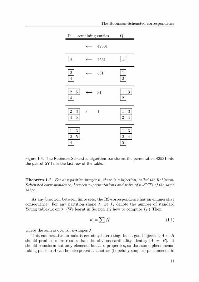
Now we are ready to describe the Robinson-Schensted correspondence. Let ustake any permutation, for example 42531. Our goal is to create two 5-SYTs of thesame shape: the P-tableau and the Q-tableau.

From the beginning we let the P- and Q-tableaux both be empty. Then weinsert the permutation entries into the P-tableau one by one from left to right.After each insertion we update the Q-tableau to record which square was added tothe P-tableau. More precisely, the Q-tableau is always the SYT corresponding tothe path in Young’s lattice followed by the growing shape of the P-tableau so far.After inserting all permutation entries, we have completed the Robinson-Schenstedalgorithm and obtained the P- and Q-tableaux corresponding to the permutation.

Our example permutation 42531 results in the development of the P- and Q-tableaux depicted in Figure 1.4. It is not hard to see that it is possible to runthe whole process backwards and thereby recover the permutation from the P- andQ-tableaux.

Let us write down the results of our efforts as a theorem:

10

The Robinson-Schensted correspondence

P ← remaining entries Q

← 42531

4 ← 2531 1

2

4← 531 1

2

2 5

4← 31 1 3

2

2 3

4 5← 1 1 3

2 4

1 3

2 5

4

1 3

2 4

5

Figure 1.4: The Robinson-Schensted algorithm transforms the permutation 42531 intothe pair of SYTs in the last row of the table.

Theorem 1.2. For any positive integer n, there is a bijection, called the Robinson-Schensted correspondence, between n-permutations and pairs of n-SYTs of the sameshape.

As any bijection between finite sets, the RS-correspondence has an enumerativeconsequence. For any partition shape λ, let fλ denote the number of standardYoung tableaux on λ. (We learnt in Section 1.2 how to compute fλ.) Then

n! =∑

f2λ (1.1)

where the sum is over all n-shapes λ.

This enumerative formula is certainly interesting, but a good bijection A ↔ Bshould produce more results than the obvious cardinality identity |A| = |B|. Itshould transform not only elements but also properties, so that some phenomenontaking place in A can be interpreted as another (hopefully simpler) phenomenon in

11


B. Does Robinson-Schensted live up to these expectations? As we will see in thenext section, the answer is: Yes, by far!

1.4 Properties of the RS-correspondence

Let us take some operations on permutations and see how these affect the corres-ponding P- and Q-tableaux. We will omit the proofs.

Maybe the simplest thing we can do to a permutation is reversing it, i.e. writingit backwards. On the tableau side this corresponds to transposing the P -tableau,i.e. exchanging rows and columns. (For example, the transpose of 1 2 4

3 5 is1 32 54

.) TheQ-tableau is also affected, but in a more complex way which I will not describehere.

Another simple operation on permutations is inverting, and now prepare forthe most astonishing proposition: Inverting the permutation means exchanging theP- and Q-tableaux! This magical correspondence is not at all obvious from theconstruction of the tableaux, and it has an intriguing consequence.

A permutation that is its own inverse is called an involution. Since such apermutation corresponds to P- and Q-tableaux which are equal, we get the followingtheorem.

Theorem 1.3. For any positive integer n, the Robinson-Schensted correspondencegives a bijection between n-involutions and n-SYTs.

Together with equation (1.1), the theorem above has a beautiful corollary. (Re-call that fλ is the number of SYTs on the shape λ.)

Corollary 1.1. For any positive integer n, we have

∑

f0λ = the number of n-partitions, (1.2)

∑

f1λ = the number of n-involutions = the number of n-SYTs, (1.3)

∑

f2λ = the number of n-permutations = n!, (1.4)

where the sums are over all n-shapes λ.

One may wonder whether there exists an identity of the form “∑

fkλ = some-

thing interesting” for some k other than 0,1,2. I do not know of any such result.

12

Chapter 2

About papers I and II —

sign-imbalance

2.1 Stanley’s conjecture

In October 2002 I received an e-mail from Anders Bjorner with an interesting math-ematical problem. He had just visited MIT where he had picked up a conjecture byRichard Stanley. Recall that the sign of a permutation is +1 if the number of inver-sions (wrong-order pairs) is even, and −1 if this number is odd. (The permutation3142 has three inversions — 31, 32, 42 — so it has negative sign.)

Let the sign of a standard Young tableau be the sign of the permuta-tion you get by reading it row by row from left to right, like a book.Conjecture: The sum of the signs of all n-SYTs is 2⌊n/2⌋.

I was intrigued and wrote a program that computed the contribution of each shape,and I found that the power of 2 came from the SYTs on pure hooks, i.e. shapes ofthe form k + 1 + 1 + · · ·+ 1. Then I let the problem rest for five months.

In March 2003 I began my Master’s project for Anders and I suggested Stanley’sconjecture as my subject. Anders thought it was a good idea but he warned methat it could be hard. That proved to be correct; I examined many interesting ideasbut it was not until July that I had some success. Here I will briefly describe themain methods used to attack the problem. The most interesting ones resulted inpaper I in this thesis.

In fact, in a preprint [35], Stanley had made a substantial refinement of theabove conjecture and he also presented another related conjecture about sums ofsquares of sign-imbalances. I will describe these conjectures in a moment.

First we need some definitions.

13

2. About papers I and II — sign-imbalance

Figure 2.1: The 13-shape 5 + 3 + 2 + 2 + 1 has d(λ) = 2 and v(λ) = h(λ) = 5. Theshaded squares form the fourling body.

Definition 2.1. The sign-imbalance Iλ of a partition shape λ is the sum of thesigns of all SYTs on λ. If the sign-imbalance vanishes we say that the shape issign-balanced.

Note that the sign-imbalance of a shape is essentially independent of the readingorder in the definition of the sign of a tableau. Changing the reading order (e.g. toJapanese column-wise book reading order) may alter the sign of a SYT, but thenthe sign of every SYT on the same shape is altered. Thus, for any shape, theparticular reading order only affects the sign of its sign-imbalance.

A 2× 2-square is called a fourling and the maximal number of disjoint fourlingsthat fit in the shape λ is denoted by d(λ). The maximal number of disjoint hori-zontal dominoes that fit inside λ is denoted by h(λ) and the maximal number ofvertical dominoes is denoted by v(λ). Figure 2.1 shows an example.

Now Stanley’s conjectures can be formulated as identities of generating func-tions. (We let λ ⊢ n denote that λ is an n-shape.)

Conjecture 2.1 (Stanley, 2002).

(a) For every n ≥ 0,

∑

λ⊢n

qv(λ)td(λ)xh(λ)Iλ = (q + x)⌊n/2⌋.

(b) If n 6≡ 1 (mod 4),∑

λ⊢n

(−1)v(λ)td(λ)I2λ = 0.

2.2 Unsuccessful methods

There were plenty of conceivable methods to prove the conjectures, most of whichled nowhere. I will discuss them here in about the same chronological order as Iexamined them in when I worked on the problem in 2003.

14

Unsuccessful methods

Transposition of the shape

My first idea was to figure out what happens to the sign of a tableau during trans-position. What if transposition was sign-alternating for non-hook tableaux! Thenthe 2⌊n/2⌋-conjecture would follow. Unfortunately the situation is more complexand whether the sign will change depends on d(λ), the number of fourlings that fitin the shape.

Proposition 6.6 in paper I says that, for any shape λ, the sign-imbalance of thetransposed shape λ′ is Iλ′ = (−1)d(λ)Iλ. If λ′ = λ and d(λ) is odd, we concludethat λ is sign-balanced. For instance, this is the case when λ is an m ×m-squarewith m congruent to 2 or 3 modulo 4.

The domino approach

A promising observation that most people will make is the reduction to dominotableaux: the sign-imbalance of a shape equals the sum of the signs of all dominotableaux of that shape. A domino tableau is a standard Young tableau where, forall odd i, the entries i and i + 1 are in adjacent squares, forming a horizontal orvertical domino.

I intentionally avoided following this track because of the great amount of re-search that had been put into this approach without solving the problem.

But then it happened: In May 2003, Anders told me that one of Stanley’sstudents, Thomas Lam, had proved part (a) of the conjecture! Lam hadn’t hadthe time to write down his proof yet, but according to the rumour it made useof a theory of symmetric functions involving domino tableaux. Later on, whenLam’s preprint [20] was made available in August 2003, it turned out that he usescombinatorial methods rather similar to the ones in paper I, but based on dominotableaux.

Pocketing my disappointment, I decided to continue looking for a proof of part(b) of the conjecture and possibly a simpler proof of part (a).

The RS-bijection between SYTs and involutions

Another promising method I tried was the classical bijection between SYTs andinvolutions, Theorem 1.3. Maybe the sign property in tableau space would have anice representation in involution space. I managed to establish the connection forhook tableaux but in spite of several computer analyses I failed to find a generalpattern.

Later, as is shown in paper I, it turned out that the sign of the involution doesnot say anything about the sign of the tableau, it merely keeps track of the parityof the number of vertical dominoes that fit in the shape. More precisely, the signof the involution equals (−1)v(λ), where λ is the shape of the corresponding SYT.(This is also a simple consequence of a theorem by Schutzenberger stating that the

15


number of fixpoints of the involution equals the number of columns of λ of oddlength.)

Lattice paths

A SYT on a shape λ = λ1 + λ2 + · · · can be viewed as a lattice path in Z∞ from(0, 0, . . .) to (λ1, λ2, . . .) without crossing any of the planes xi+1 = xi. I put in a lotof effort to solve the problem in the space of lattice paths, but without success.

2.3 A stronger conjecture

A little imagination and heavy computational analysis lead to a sharpening of bothparts of Stanley’s conjecture. Finally I had a result! Chess tableaux instead ofdomino tableaux and general RS-insertion instead of the involution-tableau bijec-tion put the pieces together.

The statistic d(λ) counts the fourlings that fit inside λ, but it does not careabout how these fourlings fit. A shape consisting of disjoint fourlings is called afourling shape. If we pack d(λ) disjoint fourlings inside λ as close to the north-westcorner as possible, these fourlings form a subshape of λ called its fourling body. Inother words, the fourling body of a shape is its largest fourling subshape. Lookagain at Figure 2.1 for an example.

In paper I, I show the following theorem which implies part (a) of Conjecture 2.1once one knows that the right-hand side (q + x)⌊n/2⌋ comes from the hook shapes(the shapes with empty fourling body); this is proved twice by Stanley in [35] andonce by me in paper I.

Theorem 2.1. Given a non-empty fourling shape D and nonnegative integers h,v and n, we have

∑

Iλ = 0

where the sum is taken over all n-shapes λ with fourling body D, h(λ) = h, andv(λ) = v.

Figure 2.2 shows an example.

In the same spirit, in paper I we have the following theorem which is a sharpeningof part (b) of Conjecture 2.1 for even n. (The odd case is also settled in paper I,but we omit the details here.)

Theorem 2.2. Given a fourling shape D and an even positive integer n, we have

∑

(−1)v(λ)I2λ = 0

where the sum is taken over all n-shapes λ with fourling body D.

16

Chess tableaux

5 5 2 2

−5 −2 −7

Figure 2.2: The sign-imbalances of the 12-shapes λ with fourling body andv(λ) = h(λ) = 5. You can check that their sum vanishes.

Figure 2.3: A chess colouring of the shape 5 + 3 + 2 + 2 + 1.

2.4 Chess tableaux

Each of Theorem 2.1 and 2.2 implies that non-empty fourling shapes are sign-balanced. This fact is surprisingly hard to prove, and the usual reduction to dominotableaux does not simplify matters. Stanley [35, Cor. 2.2] gives a proof using thepromotion and evacuation operators (jeu de taquin) originally defined by Schutzen-berger.

In paper I, I introduce a concept called chess tableaux which makes sign-balanceof fourling shapes almost transparent. Given any shape, colour its squares blackand white as a chessboard, with the north-west corner being black; see Figure 2.3.A chess tableau is a SYT with odd entries in black squares and even in white.

It is easy to find a sign-reversing involution on non-chess tableaux, showing thatthe sign-imbalance of a shape equals the sum of the signs of all chess tableaux onthat shape. Clearly, the shape of a chess tableau has equally many black as whitesquares, or one more black square. Suddenly we are able to identify a large classof sign-balanced shapes, namely those with a skew distribution of white and blacksquares. Unfortunately, the fourling shapes do not belong to this class — they have

17


indeed equally many black as white squares. But in a SYT on a non-empty fourlingshape, the largest entry is even, so if the SYT is a chess tableau this entry shouldbe in a white square. But all south-east corners of a fourling shape are black! Thus,there are no chess tableaux on a non-empty fourling shape and we conclude that itis sign-balanced.

2.5 Sign under the Robinson-Schensted correspondence

With all due deference to chess tableaux and fourling shapes, Stanley’s conjecturewould not have been settled without the Robinson-Schensted correspondence. Thefollowing charming formula for the transformation of sign under the RS-bijectionappears in paper I (and was found independently by Reifegerste [28]).

Proposition 2.1. Under the RS-correspondence π ↔ (P, Q) we have

sgn π = (−1)v(λ) sgnP sgnQ

where λ is the shape of P and Q.

Recall our example from Figure 1.4:

42531↔ (1 32 54

,1 32 45

)

Here, sgn 42531 = −1, sgnP = sgn13254 = +1, and sgnQ = sgn13245 = −1. Theshape of P and Q has room for two vertical dominoes, so (−1)v(λ) = +1.

As a simple consequence of Proposition 2.1, we obtain the following theorem,which is simultaneously a specialisation and a generalisation of Conjecture 2.1(b).

Theorem 2.3. For all n ≥ 2,

∑

λ⊢n

(−1)v(λ)I2λ = 0.

2.6 Skew partitions shapes and paper II

In 1990 Sagan and Stanley [29] introduced analogues of the Robinson-Schenstedalgorithm for skew tableaux. In paper II, I investigate how the sign property istransferred by the skew RS-correspondence, resulting in a remarkably simple gen-eralisation of the ordinary non-skew formula. From this I am able to deduce thefollowing skew analogue to Theorem 2.3 above.

Theorem 2.4. Let α be a fixed partition shape and let n be a positive even integer.Then

∑

λ/α⊢n

(−1)v(λ)I2λ/α =

∑

α/µ⊢n

(−1)v(µ)I2α/µ.

For odd n there is a similar formula in paper II.

18

What has happened since the publication of papers I and II?

2.7 What has happened since the publication of papers I

and II?

Another conjecture

In 2001 Dennis White [39] computed the sign-imbalance of rectangular shapes. Tostate his result and a related conjecture we need a couple of definitions.

Let µ = µ1 + µ2 + · · ·+ µℓ be a partition shape with µ1 > µ2 > · · · > µℓ ≥ 0. Iffor each i = 1, 2, . . . , ℓ the ith row of µ is shifted i− 1 steps to the right, the resultis called a shifted shape and is denoted by µ = (µ1, µ2, . . . , µℓ). A shifted tableauon µ is just what you would guess: a filling of the squares with integers 1, 2, . . . , N(where N is the number of squares) such that every row and column is increasing.Let gµ denote the number of shifted tableaux on µ.

Now White’s result can be stated: If m ≥ n ≥ 2, the m × n rectangle is sign-balanced unless m+n is odd in which case the sign-imbalance is ±gµ for the shiftedshape µ = (k, k − 1, . . . , k − n + 1), where k = (m + n− 1)/2.

It is natural to ask if there is a generalisation of White’s result to non-rectangularshapes. Soon after the completion of paper I, Stanley updated his preprint [35] onthe ArXiv and added a conjecture due to A. Eremenko and A. Gabrielov whichis still open. Define the sum of two shifted shapes µ = (µ1, . . . , µℓ) and ν =(ν1, . . . , νℓ) by µ + ν = (µ1 + ν1, . . . , µℓ + νℓ), and define multiplication by a scalart by tµ = (tµ1, . . . , tµℓ) if this is a shifted shape.

Conjecture 2.2 (Eremenko and Gabrielov, 2003). If we fix the number ℓ of parts(i.e. rows) and parity of each part of a partition shape λ, then there are integersc1, . . . , ck and integer vectors γ1, . . . , γk ∈ Zℓ such that

Iλ =

k∑

i=1

cig12(λ+γi).

For instance, it can be verified that I(2a+1,2b,2c) = g(a,b,c) + g(a+1,b−1,c).

Counting chess tableaux

When using chess tableaux to compute sign-imbalance, some tableaux contributeto the sum by +1 and others by −1. But what happens if we forget about sign-imbalance for a moment and let all chess tableaux contribute positively to the sum?

Open question 2.1. How many chess tableaux are there on a given shape?

In 2005 Timothy Y. Chow, Henrik Eriksson and C. Kenneth Fan [8] answered thequestion for shapes with at most three rows. For instance, the number of chesstableaux on a 3× n rectangle is

2

(n− 1)n2

n−2∑

k=0

(

n

k

)(

n

k + 1

)(

n

k + 2

)

.

19


Chow, Eriksson and Fan also apply chess tableaux as a tool for solving a certaintype of chess problems!

Sign-imbalance as a lower bound for the number of real solutions

to polynomial equations

In 2005 Evgenia Soprunova and Frank Sottile [31] found a truly unexpected ap-plication of sign-imbalance. To any partition shape they associate a system ofpolynomial equations quite naturally. Then they show that the absolute value ofthe sign-imbalance of the shape is a lower bound for the number of real solutionsto the equation system! (To be fair, their results are much more general and workfor any poset, but for simplicity we restrict ourselves to partition shapes in thispresentation.)

I will illustrate the findings of Soprunova and Sottile by an example. Let λ bethe 5-shape 3 + 1 + 1 and put 5 indeterminates, say x, y1, y2, z1, z2, in the squaresof λ, like this:

x y1 y2

z1

z2

Now, for every subshape µ of λ we multiply the indeterminates contained in µto obtain a square-free monomial. In our example there are 10 such subshapemonomials, including the empty subshape monomial 1 and the maximal subshapemonomial xy1y2z1z2. We arrange the 10 monomials according to degree, and writedown equations of the form

c0 + c1x + c2(xy1 + xz1) + c3(xy1y2 + xy1z1 + xz1z2)

+ c4(xy1y2z1 + xy1z1z2) + c5xy1y2z1z2 = 0.

where c0, . . . , c5 are real numbers. Any system of 5 such equations (corresponding to5 different choices of c0, . . . , c5) has at most fλ isolated solutions in (C\{0})5, wherefλ is the number of SYTs on λ. (This follows from Kushnirenko’s Theorem [19]together with [32, Cor. 4.2].) Soprunova and Sottile show that there are at least|Iλ| = 2 real solutions.

To gain as much as possible from this result, I would like to pose the followingnatural question:

Open question 2.2. Which n-shape has the largest sign-imbalance?

(Of course, to maximise the sign-imbalance among n-element posets would be evenbetter, but let us stick to partition shapes.) There seems to be nothing on thisproblem in the literature, not even partial results. The related problem of findingthe n-shape with the greatest number of SYTs on it was solved (at least asymp-totically) already in 1977 independently by B. F. Logan and L. A. Shepp [25], and

20

What has happened since the publication of papers I and II?

by A. M. Vershik and S. V. Kerov [38]; see also [34, Exerc. 7.109.e, p. 488]. Theirmethod can be described like this: Take the logarithm of the hook length formula toget a sum instead of a hook length product. When n tends to infinity the sum is wellapproximated by an integral. Now, solve the corresponding variational problem!

Unfortunately, there is no known equivalent of the hook length formula for sign-imbalance, so an entirely different approach is required in this case.

New proofs of sign-imbalance theorems

In July 2006, one year after the preprint publication of paper II, Thomas Lamwrote the note [21], “On Sjostrand’s skew sign-imbalance identity”, where he givesan alternative proof of Theorem 2.4. He uses domino tableaux and a generating-function identity called the skew domino Cauchy identity.

More recently, in November 2006, Lam put the preprint [22], “Signed differen-tial posets and sign-imbalance”, on the ArXiv. There he defines signed differentialposets, a signed version of differential posets introduced by Stanley [33] and inde-pendently by Fomin [12] back in 1988. Lam shows that Young’s lattice (with propersigns) is a signed differential poset, and that Stanley’s original 2⌊n/2⌋-conjecture(i.e. Conjecture 2.1(a) with q = t = x = 1) and our Theorem 2.3 result from thesigned differential poset structure. In this framework he also gives a third proof ofTheorem 2.4.

21

Chapter 3

About paper III — skyscraper

exercise and monkey bars

3.1 The story

You live in a skyscraper Z. In the morning you get your exercise by climbing outthrough the window, following 5n one-way ladders, and climbing into your apart-ment again. At each level there is one ladder going 3 levels up and another laddergoing 2 levels down. Once you have climbed up from a level you are committed,for the rest of that morning, to always choose the climb-up option should you visitthat level again. In how many ways can you perform your exercise?

In the summer 2005, Nick Loehr and Greg Warrington studied the problemabove and conjectured that the answer is 10n. Kimmo Eriksson once claimed thatsimple statements of this kind must be either (1) false, (2) already proved by Euler,or (3) both. But as it turned out, the Loehr-Warrington 10n conjecture does notbelong to any of these categories, and it is certainly not trivial to prove. It is atruly amazing conjecture!

Or was. Well, it is definitely still amazing, but it is not a conjecture anymore.In September 2005 Shalosh B. Ekhad, Vince Vatter and Doron Zeilberger put thepaper “A proof of the Loehr-Warrington amazing TEN to the power n conjecture”[11] on the ArXiv. Vatter and Zeilberger taught Zeilberger’s computer ShaloshB. Ekhad a few tricks and then Ekhad worked for 30 seconds and automaticallyconstructed a formal proof of the conjecture.

So was that the end of the story? No, not at all, that was just the beginning.The real story is that the Loehr-Warrington 10n conjecture was delivered in asignificantly more general package already from the start: Let a and b be anyrelatively prime positive integers and replace 5n by (a+ b)n and 3 and 2 by a and bin the skyscraper setting above. Then the conjectured number of exercise climbingpaths is

(

a+ba

)n. Ekhad showed only the special case a = 3, b = 2, so the general

problem was still wide open, and even for Ekhad’s 3,2-case the task of finding a

23

3. About paper III — skyscraper exercise and monkey bars

human proof remained. Not that human proofs are better than computer generatedin principle, but this particular problem deserves a simple and beautiful solution.

In October 2005, Loehr and Warrington wrote a paper together with BruceE. Sagan called “A human proof for a generalization of Shalosh B. Ekhad’s 10n

Lattice Paths Theorem” [23]. There they proved the conjecture when b = 2 and ais any odd positive integer. (In fact they show a slightly stronger proposition, butI am trying to keep things simple in this overview.)

Inspired by both the electronic and the human achievements above, I am proudto present a combinatorial proof of the full Loehr-Warrington 10n conjecture inpaper III of this thesis.

3.2 What has happened since the publication of paper III?

After Doron Zeilberger had read my proof he wrote to Martin Aigner and GunterZiegler and nominated it to be included in the next edition of Proofs from THEBOOK [1]. The famous Hungarian mathematician Paul Erdos imagined a semi-divine book called THE BOOK, in which only the most appealing and profoundmathematical proofs are included. In Proofs from THE BOOK, now released innine languages, Aigner and Ziegler have compiled a collection of beautiful proofsfrom Euclid to modern times, all of which use only basic higher mathematics. It isdoubtful that my proof would qualify for a position in this prestigious volume (andof course there is also the possibility that there will be no further editions) but inall cases I am glad my work is being appreciated.

Zeilberger has written a paper about my paper which he calls “Another Proofthat Euler Missed: Jonas Sjostrand’s Amazingly Simple (and Lovely!) Proof ofthe No-Longer-So-Amazing Loehr-Warrington Lattice Paths Conjecture” [40]. Itcontains a very nice popular description of the bijections in paper III. With Doron’spermission I include it here in an unabridged version.

24

What has happened since the publication of paper III?Another Proof that Euler Missed: Jonas Sj�ostrand's Amazingly Simple (and Lovely!) Proofof the No-Longer-So-Amazing Loehr-Warrington Latti e Paths Conje tureDoron ZEILBERGER1A few months ago Ni k Loehr and Greg Warrington made a seemingly amazing onje ture. Leta and b be relatively prime positive integers and let n be a positive integer. There are exa tly�a+bb �n latti e paths from (0; 0) to (nab; nab), with fundamental steps (a; 0) and (0; b), that obeythe following ondition:Whenever you have made a horizontal step (x; y) ! (x + a; y) you are ommitted, for ever after,to always hoose the horizontal-step option should you visit a site of the form (x+ jab; y+ jab) forsome j > 0.Being a wordy kind of guy, I immediately translated this to a problem on words, in the alphabetfa;�bg, avoiding fa tors of the form a[�a℄(�b) where [�a℄ denotes a word that sums to �a. Thisbrings to mind Goulden-Ja kson, alas, with in�nitely many `mistakes'. Even though the languageis no longer regular, its onje tured rational generating fun tion suggested that it has a lineargrammar, and being a dis iple of Mar o S h�utzenberger, I tried to look for a linear grammar.Helped by my brilliant human dis iple Vin e Vatter, and my ele troni dis iple Shalosh B. Ekhad,we found su h a grammar for the ase a = 3 and b = 2. The same method should, in prin iple,yield a proof for every spe i� a and b, but Shalosh's memory only suÆ ed for this ase. This waswritten up in [EVZ℄. A human, latti e-path, proof of the more general b = 2 ase appeared shortlyafter [LSW℄. But neither the linguisti approa h of the former nor the latti e-path approa h of thelatter were the right way. It was the mathemati al epsilon (Ph.D. student) Jonas Sj�ostrand whogave the oup de gra e to the general onje ture [S℄ by realizing that the natural habitat of thisproblem is Graph Theory 101, in fa t a variant of its inaugural theorem, Euler's K�onigsbergBridge Theorem.Imagine a monkey limbing up and down, but always ounter- lo kwise, ylindri al monkey-barsof perimeter (a+ b) with one of the verti al olumns painted red and designated the 0- olumn. Atany point, the monkey an go either a units up or b units down to its immediate ounter- lo kwise-neighboring olumn. It starts and ends at the same spot (let's all it the origin). The awkwardLoehr-Warrington ondition now translates to the natural ondition that whenever it leaves a pointin the upwards dire tion, all subsequent exits from that point (if they exist) must be upwards aswell.If the monkey travels with a string, and tapes it to ea h visited site (and draws arrows in the1 Department of Mathemati s, Rutgers University (New Brunswi k), Hill Center-Bus h Campus, 110 FrelinghuysenRd., Pis ataway, NJ 08854-8019, USA. zeilberg at math dot rutgers dot edu ,http://www.math.rutgers.edu/~zeilberg . Ex lusively published in the Personal Journal of Ekhad and Zeil-berger http://www.math.rutgers.edu/~zeilberg/pj.html . First version: O t. 23, 2005. A ompanied by Maplepa kage JONAS downloadable from Zeilberger's website. Supported in part by the NSF.125

3. About paper III — skyscraper exercise and monkey barsappropriate dire tions), he would naturally tra e a dire ted graph with multiple edges. It is easyto see that it an never visit higher points than the starting point on the red olumn. By onstru tion, the monkey has travelled a Eulerian y le in the graph that he has just made, andhen e it is a Eulerian dire ted graph, with the obvious ne essary ondition that it is balan ed:ea h vertex has as many in oming edges as outgoing edges. This brings to mind the `easy part' of(the dire ted version of) Euler's Seven Bridges of K�onigsberg Theorem. But the `hard' part (whi his almost as easy) that if a dire ted graph is balan ed, then it has a Eulerian y le, goes almostverbatim. Re all that Fleury's algorithm �nds a Eulerian y le by avoiding bridges if it an. If yourepla e `don't go over a bridge unless you have no other hoi e' by `don't go up unless you have noother hoi e' you would get the unique Eulerian y le that Ni k and Greg would approve of. Sothere is a natural bije tion between su h legal downwards-greedy monkey iteneraries and su h onne ted Eulerian graphs, for whi h the origin is the highest visited site on the red olumn.That's very ni e, but how do we get �a+ba �n? Easy! On e the �rst monkey formed the Euleriangraph, let another monkey also tra e a downwards-greedy y le but now starting, not at the origin,but at the lowest visited site on the red olumn. Sin e this is the lowest point, it will return toit after exa tly (a+ b) steps, forming a lap i.e. a minimal good y le of length a+ b, the number ofwhi h are �a+ba �. Removing the edges of this lap will not ruin Eulerianity and the other ondition,and we get a legal su h graph with (n� 1)(a+ b) edges, and we an ontinue re ursively. It is also lear how to go ba k. Given su h a Sj�ostrand Eulerian graph, and a lap- y le, �nd the lowest pointin the red olumn su h that if we insert that lap there it will be onne ted to our graph.If you don't believe Jonas, he k out my Maple pa kage JONAS available from my website. Inparti ular try out pro edures J12,J21,J23,J32.Remarks. 1. The proof is all Jonas's but the analogy to Fleury's algorithm and the monkeyrendition are mine. 2. Jonas's proof only slightly detra ts from the interest of the Ekhad-Vatter-Zeilberger original spe ial ase, sin e, �rst and foremost, it is a ase-study of ompletely automati yet rigorous experimental mathemati s, but also be ause the method an be applied to dis overand prove linear grammars for many other languages for whi h we are not so lu ky to have a graph-theoreti al formulation. 3. Jonas Sj�ostrand's brilliant tri k may be summarized as follows:If you are stumped proving that A � B �nd a set C su h that both A � C and C � B are natural.Referen es[EVZ℄ S.B. Ekhad, V. Vatter and D. Zeilberger, A Proof of the Loehr-Warrington Amazing TENto the power n Conje ture, preprint, available from the authors' websites.[LSW℄ N. Loehr, B. Sagan, and G. Warrington, A Human Proof for a Generalization of Shalosh B.Ekhad's 10n Latti e Paths Theorem, preprint, available from arXiv.org .[S℄ J. Sj�ostrand, Cylindri al Latti e Paths and The Loehr-Warrington Ten to the Power N Conje -ture, preprint, available from arXiv.org . 226

What has happened since the publication of paper III?

Cylindrical lattice walks and partition shapes

Paper III has an obvious enumerative flavour, but to match the title of this thesis,it had better have something to do with partition shapes as well. As the paper iswritten it is far from obvious that such a connection exists. Fortunately, Loehr andWarrington have taken care of this. In a recent paper [24], they use the Euleriancycle construction from paper III to give the first combinatorial proof of an attract-ive partition identity originally due to Mark Haiman. Essentially, what they do isto interpret a cylindrical monkey itinerary as a lattice walk in the plane which inturn constitutes the south-east border of a partition shape. I will not discuss theirmethod further here, but merely state Haiman’s identity.

There is a well-known generating function that enumerates partition shapes λby area, |λ|, and number of rows, ℓ(λ):

∑

all shapes λ

q|λ|tℓ(λ) =

∞∏

i=1

1

1− tqi. (3.1)

If we transpose a shape λ 7→ λ′, its original number of rows ℓ(λ) becomes the lengthof the first row, λ′

1. Thus the following “transposed”variant of Equation (3.1) holdstoo:

∑

all shapes λ

q|λ|tλ1 =∞∏

i=1

1

1− tqi. (3.2)

As we will see, Haiman showed that there is a continuous spectrum of statisticsh+

x (λ) that varies from ℓ(λ) to λ1 when the real number x goes from 0 to ∞. Thevery same generating function enumerates partitions by any of those statistics!

Recall that, for a square s in a shape, the leg length l(s) is the number of squaresbelow s in the same column and the arm length a(s) is the number of squares tothe right in the same row. Now, for any shape λ and any real x ≥ 0, let h+

x (λ)denote the number of squares s in λ such that

a(s)

l(s) + 1≤ x <

a(s) + 1

l(s).

Also, let h−x (λ) denote the number of squares s in λ such that

a(s)

l(s) + 1< x ≤

a(s) + 1

l(s).

In these formulas, a fraction with a zero denominator is interpreted as +∞. Nowwe can state Haiman’s result which Loehr and Warrington prove combinatorially.

Theorem 3.1 (Haiman). For all real x ∈ [0,∞),

∑

all shapes λ

q|λ|th+x (λ) =

∞∏

i=1

1

1− tqi.

27

3. About paper III — skyscraper exercise and monkey bars

For all x ∈ (0,∞],∑

all shapes λ

q|λ|th−

x (λ) =

∞∏

i=1

1

1− tqi.

The classical equations (3.1) and (3.2) follows from Theorem 3.1 by puttingx = 0 and x =∞.

28

Chapter 4

Preliminaries to paper IV

4.1 Permutations and rook polynomials

In chess there is a chessman called rook which can capture other chessmen in thesame rank or file (i.e. row or column). A classical popular puzzle asks in how manyways eight rooks can be placed on a chessboard so that no two of them can captureeach other. The answer is of course 8! = 40320.

A configuration of n rooks on an n by n board with exactly one rook in everyrow and column decodes an n-permutation π such that π(i) = j if and only ifthere is a rook in row i and column j. As in the preceding chapters, we willwrite permutations in one-row notation π = π(1)π(2) · · · π(n). Figure 4.1 shows anexample.

The rook diagram is a very concrete interpretation of a permutation, and themost common operations can easily be described in terms of rook diagrams. Invert-ing the permutation (as a function) simply means transposing the rook diagram,i.e. exchanging rows and columns, or reflecting in the main diagonal. Reversingthe permutation (writing it backwards) means reflecting the rook diagram upsidedown.

On an n by n board there are n! configurations of n rooks, and it is easy to

Figure 4.1: The rook diagram of the permutation 35124.

29

4. Preliminaries to paper IV

see that there are(

n(n − 1) · · · (n − k + 1))2

/k! configurations of k rooks. Thingsbecome more complicated if we allow for more peculiar boards, possibly containingholes or even separate components.

In the following exposition, a board A is a zero-one matrix, with ones corres-ponding to squares and zeroes corresponding to holes. (So the full n by n squareboard is represented by the n by n matrix with ones everywhere.) A rook configur-ation on A is a placement of rooks on the one-entries of A, no two in the same rowor column. We define the kth rook number of A, denoted by RA

k , as the number ofrook configurations on A with k rooks.

Now, it is tempting to define the rook polynomial as∑n

k=0 RAk xk and hope for

some magical factorization of this expression. However, this polynomial does notfactorize nicely, not even for a square board! The falling factorial n(n− 1) · · · (n−k+1) that occurred above turns out to be highly relevant for the computation of RA

k

in general, and this is incorporated in the “right”definition of the rook polynomial:

Definition 4.1 (Goldman et al. [15]). For any nonnegative integer n and any boardA, the nth rook polynomial of A is defined by

RAn (x) =

n∑

k=0

RAn−kx(x− 1) · · · (x− k + 1).

As we will see, in this form the rook polynomial is computable in many cases, andthe main reason for success is the following interpretation of the rook polynomial:If A has n rows and x is a large integer (no less than n), the rook polynomial RA

n (x)evaluates to the number of configurations of n rooks on the rectangular board (AJ),where J is an n by x matrix with ones everywhere. From this observation, it followseasily that the nth rook polynomial of the full n by n square board is

Rn × n all-ones matrix

n (x) = (x + 1)(x + 2) · · · (x + n).

An interesting feature of Definition 4.1 is the parameter n that determines thematching of “basis functions”x(x−1) · · · (x−k+1) and“coordinates”RA

n−k. Some-times it is necessary to lower or raise the value of n, and for this purpose there isa simple equation relating the nth and (n + 1)st rook polynomial:

RAn+1(x) = RA

n+1 + xRAn (x− 1). (4.1)

It is also of interest to convert between the basis of falling factorials and the basisof power functions. Namely, we have

xj =

j∑

i=0

Sj,ix(x− 1) · · · (x− i + 1),

x(x − 1) · · · (x− j + 1) =

j∑

i=0

sj,ixi,

(4.2)

where sj,i and Sj,i are Stirling numbers of the first and second kind, respectively.

30

Permutations and rook polynomials

Figure 4.2: To the left is the Aztec diamond of order 4. After suitable permutations ofrows and columns, its complementary shape becomes an Aztec diamond of order 3 asshown in the right picture.

The rook reciprocity theorem

One of the most elegant result on rook polynomials is the following formula, whichrelates the rook polynomials of a board and its complementary board.

Theorem 4.1 (The rook reciprocity theorem). For any n by n board A, we have

RAn (x) = (−1)nRA

n (−x− 1),

where A is the complementary board to A, obtained by substituting ones for zeroesand zeroes for ones.

For an elegant proof, I refer to Timothy Chow [7].

As an example of an application of the rook reciprocity theorem, let us computethe 2mth rook polynomial of an Aztec diamond Azm of order m; see Figure 4.2.Observe that the rook polynomial is invariant under permutations of rows andcolumns of the board. It is not hard to see that the complementary board tothe Aztec diamond of order m is an Aztec diamond of order m − 1 after properpermutations of rows and columns. Hence, by the rook reciprocity theorem we get

RAzm

2m (x) = RAzm−1

2m (−x− 1).

Now, we would like to iterate the procedure to obtain smaller and smaller Aztecdiamonds until we reach a trivial one. The problem is that the complementaryAztec diamond Azm−1 is embedded in a matrix of dimensions 2m × 2m, so if wetake the complement of it we would just get a larger Aztec diamond Azm back again.This is easily fixed by just shrinking the matrix to dimensions 2(m− 1)× 2(m− 1),but to be able to use the rook reciprocity theorem again, we now have to rewritethe rook polynomial R

Azm−1

2m (−x − 1) in terms of the 2(m − 1)th rook polynomial

31


Figure 4.3: Diagrams of the left-aligned Ferrers matrix λ =(

1 1 1 01 1 0 00 0 0 0

)

and the right-

aligned Ferrers matrix µ =(

1 1 11 1 10 0 1

)

.

RAzm−1

2(m−1)(−x− 1). By applying Equation (4.1) twice (and observing that RAzm−1

2m−1 =

RAzm−1

2m = 0), we obtain

RAzm−1

2m (−x− 1) = (x + 1)(x + 2)RAzm−1

2(m−1)(−x− 3).

Finally, iteration of the above procedure yields the 2mth rook polynomial of theAztec diamond of order m,

RAzm

2m (x) = (x + 1)m(x + 2)m.

Rook polynomials of Ferrers boards

A zero-one matrix λ is a left-aligned resp. right-aligned Ferrers matrix (or Ferrersboard) if every one-entry has one-entries directly to the left (resp. to the right) andabove it (provided these entries exist). Figure 4.3 shows an example.

For Ferrers matrices, the rook polynomial can be computed by the followingtheorem.

Theorem 4.2 (Goldman et al. [15]). For a left-aligned m by n Ferrers matrix λ,

Rλn(x) =

n∏

j=1

(x + cj(λ) + j − n),

where cj(λ) is the number of ones in column j of λ.

As an example of an application of this theorem, we consider the Aztec diamondagain. By permuting the rows and columns of the Aztec diamond of order m, itis indeed possible to obtain a left-aligned Ferrers matrix. It has the cj-values2m, 2m, 2m − 2, 2m − 2, . . . , 4, 4, 2, 2 so Theorem 4.2 yields the rook polynomialRAzm

2m (x) = (x + 1)m(x + 2)m, just as expected.

q-analogues

A q-analogue is a mathematical object parameterised by a quantity q, that general-ises a known object and reduces to that object when q → 1. The “object” is usually

32

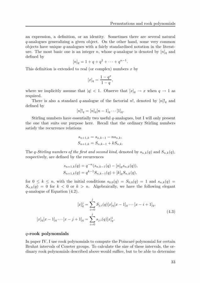
Permutations and rook polynomials

an expression, a definition, or an identity. Sometimes there are several naturalq-analogues generalizing a given object. On the other hand, some very commonobjects have unique q-analogues with a fairly standardised notation in the literat-ure. The most basic one is an integer n, whose q-analogue is denoted by [n]q anddefined by

[n]q = 1 + q + q2 + · · ·+ qn−1.

This definition is extended to real (or complex) numbers x by

[x]q =1− qx

1− q,

where we implicitly assume that |q| < 1. Observe that [x]q → x when q → 1 asrequired.

There is also a standard q-analogue of the factorial n!, denoted by [n]!q anddefined by

[n]!q = [n]q[n− 1]q · · · [1]q.

Stirling numbers have essentially two useful q-analogues, but I will only presentthe one that suits our purpose here. Recall that the ordinary Stirling numberssatisfy the recurrence relations

sn+1,k = sn,k−1 − nsn,k,

Sn+1,k = Sn,k−1 + kSn,k.

The q-Stirling numbers of the first and second kind, denoted by sn,k(q) and Sn,k(q),respectively, are defined by the recurrences

sn+1,k(q) = q−n(sn,k−1(q)− [n]qsn,k(q)),

Sn+1,k(q) = qk−1Sn,k−1(q) + [k]qSn,k(q),

for 0 ≤ k ≤ n, with the initial conditions s0,0(q) = S0,0(q) = 1 and sn,k(q) =Sn,k(q) = 0 for k < 0 or k > n. Algebraically, we have the following elegantq-analogue of Equation (4.2).

[x]jq =

j∑

i=0

Sj,i(q)[x]q [x− 1]q · · · [x− i + 1]q,

[x]q[x− 1]q · · · [x− j + 1]q =

j∑

i=0

sj,i(q)[x]iq .

(4.3)

q-rook polynomials

In paper IV, I use rook polynomials to compute the Poincare polynomial for certainBruhat intervals of Coxeter groups. To calculate the size of these intervals, the or-dinary rook polynomials described above would suffice, but to be able to determine

33


the complete Poincare polynomial we need to keep track of the number of inversionssomehow. An inversion in a permutation is an unordered pair of rooks in the rookdiagram such that one rook is north-east of the other.

For a rook configuration A on a board A, let invA A denote the number of (notnecessarily positive) entries of A with no rook weakly to the right in the same rowor below in the same column. If A is an n by n matrix and π is an n-permutation,it is easy to see that invA π equals the number of inversions in π.

Now, we can define q-analogues to the ordinary rook numbers and rook polyno-mials, (almost) following Garsia and Remmel [13].

Definition 4.2. Given a board A and an integer k ≥ 0, the kth q-rook number isdefined by

RAk (q) =

∑

A

qinvA A,

where the sum is over all rook configurations A on A with k rooks. Given a boardA and an integer n ≥ 0, the nth q-rook polynomial of A is defined by

RAn (x; q) =

n∑

k=0

RAn−k(q)[x]q [x− 1]q · · · [x− k + 1]q.

For the full n by n square board, the nth q-rook number equals [n]q! just aswe want. But it gets much better than that: Theorem 4.2, which is astonishingalready by itself, is still valid if we q-ify it properly!

Theorem 4.3 (Garsia and Remmel). For a left-aligned m by n Ferrers matrix λ,

Rλn(x; q) = qz

n∏

j=1

[x + cj(λ) + j − n]q,

where cj(λ) is the number of one-entries in column j of λ, and z is the total numberof zero-entries of λ.

Observe, however, that while the ordinary rook polynomial is invariant underpermutation of rows and columns, this is not the case for q-rook polynomials. In thissense, Theorem 4.3 is more limited than its q = 1 specialisation, Theorem 4.2. Forexample, the Aztec diamond whose rook polynomial was computed by Theorem 4.2,cannot be handled by Theorem 4.3.

Unfortunately, the rook reciprocity theorem (Theorem 4.1) has no known q-analogue, so we cannot find the q-rook polynomial of an Aztec diamond by takingcomplements either. It is easy to show that the 2mth q-rook number of the Aztecdiamond of order m is qm(m−1)(1+q)m, but the full q-rook polynomial is not known.

Open question 4.1. What is the q-rook polynomial of the Aztec diamond of orderm?

34

Coxeter groups

6

?

�

-�R

I ?180◦

?90◦

?90◦

id x y yxy xyx xyxy xy yx

Figure 4.4: The automorphism group G� of a square is generated by x and y.

4.2 Coxeter groups

Consider a square-shaped card. We will investigate its automorphism group, i.e. thegroup of all operations we can apply to the card without changing its shape andalignment. There are four possible reflections: horizontal, vertical, and two diag-onal; and three rotations: 90 degrees clockwise, 90 degrees counterclockwise, and180 degrees. Finally, there is the identity operation id which does nothing to thecard.

Let x and y denote reflection in a horizontal axis and in the main diagonal,respectively. If we first perform x and then y, the net result xy is a 90 degreeclockwise rotation. In fact, it turns out that all other operations can be performedusing only x and y, as shown in Figure 4.4. We say that the group is generated by xand y. Now, let us examine which relations these generators satisfy. As reflectionsthey obviously have order two, i.e. x2 = y2 = id. Since xy is a 90 degree rotationwhich must be performed four times before the result is id, we get (xy)4 = id. Itcan be proved that all other relations in the group follow from the ones we alreadyhave discovered. Thus, a presentation of the automorphism group of a square is

G� = 〈x, y |x2 = y2 = (xy)4 = id〉.

What we have found is in fact a simple example of a Coxeter group, and thisparticular one is called B2 or I2(4) in the standard classification.

Here is the general definition.

Definition 4.3. A Coxeter group is a group with the following presentation:

• Generators: A finite set s1, s2, . . . , sn.

• Relations: s2i = id for all i, and (sisj)

Mi,j = id for all i 6= j, where Mis a symmetric n by n matrix with entries in {2, 3, . . .} ∪ {∞}. The case(sisj)

∞ = id is interpreted as no relation at all.

In most cases one is interested in a Coxeter group W together with a particular setS of generators. The pair (W, S) is called a Coxeter system.

A Coxeter group with generators s1, s2, . . . , sn is often represented by its Coxetergraph. This is a simple graph with vertices s1, s2, . . . , sn and an edge between si

35


and sj if Mi,j ≥ 3. If Mi,j ≥ 4 the edge is labelled by that number. For example,the group G� above has the Coxeter graph 4 .

For a thorough combinatorial exposition of Coxeter groups, I recommend thebook [3] by Anders Bjorner and Francesco Brenti.

4.3 Bruhat order

There are three natural poset structures on the elements of a Coxeter group: theright weak order, the left weak order, and the Bruhat order. To describe them weneed two more definitions.

The group elements that are conjugate to some generator are called reflections.In our running example G�, the reflections are {x, y, xyx, yxy}, just as expected.Each group element w can be written as a product of generators w = si1si2 · · · sik

.If k is minimal among all such expressions for w, then k is called the length (orrank) of w, denoted by ℓ(w).

Now we are ready to define the poset relations.

Definition 4.4. The Bruhat graph of a Coxeter system (W, S) is a directed graphwith vertex set S and a directed edge from u to w if ℓ(w) > ℓ(u) and w = ut forsome reflection t. In the Bruhat order, u ≤ w if there is a directed path from u tow in the Bruhat graph.

The apparent asymmetry in the condition w = ut is illusory, for it is equivalentto w = t′u for some reflection t′ (in fact, t′ = utu−1). If we sharpen the conditionon t in the definition to be a generator instead of any reflection, we obtain the“weak graph” and the right weak order, which is now not the same as the left weakorder defined by w = su. Figure 4.5 shows the Bruhat order and weak order ofour running example G�. Obviously, the identity element id is the unique minimalelement in W . What is not so obvious is that, if W is finite, there is also a uniquemaximal element in W , denoted by w0. Furthermore, the maps w 7→ ww0 andw 7→ w0w are antiautomorphisms of the poset W , and the map w 7→ w0ww0 is anautomorphism.

In this thesis, we will only be interested in the Bruhat order on two familiesof Coxeter groups, the symmetric groups An and the hyperoctahedral groups Bn,whose Coxeter graphs are depicted in Figure 4.6. For these groups, and for manyother Coxeter groups, there exist natural permutation representations which arevery powerful combinatorial tools.

The Coxeter system An−1 is isomorphic to the symmetric group Sn of all n-permutations with the adjacent transpositions

si = 1 · · · (i − 1)(i + 1)i(i + 2) · · ·n

as generators. The reflections correspond to general transpositions. Figure 4.7shows the Bruhat order on S3. The group multiplication is the usual compositionof functions with the permutations acting from the left.

36

Bruhat order

Bruhat graph Bruhat order

I �

O �

6

�

> 6

O

}

6 > 6}

� I

id

x y

xy yx

xyx yxy

xyxy = yxyx

id

x y

xy yx

xyx yxy

xyxy = yxyx

Left weak order Right weak order

id

x y

xy yx

xyx yxy

xyxy = yxyx

id

x y

xy yx

xyx yxy

xyxy = yxyx

Figure 4.5: The Bruhat graph and the Hasse diagrams for the Bruhat order and leftand right weak order on G�.

37


An

s1 s2 s3 sn−1 sn

Bn

s0

4

s1 s2 sn−2 sn−1

Figure 4.6: The Coxeter graphs of An and Bn.

123

213 132

231 312

321

Figure 4.7: The Hasse diagram of the Bruhat order on the symmetric group S3∼= A2.

The hyperoctahedral group Bn is represented by the rotationally symmetric 2n-permutations, i.e. permutations whose rook diagrams are unaffected by a 180 degreerotation. The generators in this representation are the adjacent transposition pairs

si = 1 · · · (i− 1)(i + 1)i(i + 2) · · · (2n− i− 1)(2n− i + 1)(2n− i)(2n− i + 2) · · · (2n)

for 1 ≤ i ≤ n − 1, together with the adjacent transposition in the center s0 =1 · · · (n− 1)(n + 1)n(n +2) · · · (2n). (For most applications it is more convenient torepresent the group Bn by signed permutations, but for our purpose the rotationallysymmetric permutations are better suited.)

There is a simple interpretation of the Bruhat order on the symmetric groupSn. For an n-permutation π ∈ Sn and i, j ∈ {1, 2, . . . , n}, let

π[i, j]def= |{a ∈ {1, 2, . . . , i} : π(a) ≥ j}|.

In other words π[i, j] is the number of rooks weakly north-east of the square (i, j)in the rook diagram for π. Now we can state a criterion for comparing two per-mutations with respect to the Bruhat order. (For a proof, see e.g. [3, Th. 2.1.5].)

Lemma 4.1. Let π and ρ be n-permutations. Then π ≤ ρ in Bruhat order if andonly if π[i, j] ≤ ρ[i, j] for all 1 ≤ i, j ≤ n.

38

Schubert varieties

4.4 Schubert varieties

Historically, the Bruhat order comes from algebraic geometry, namely as describingthe containment of Schubert varieties in flag manifolds, Grassmannians, and otherhomogeneous spaces. In this section we will get a taste of Schubert varieties bystudying the symmetric group from the geometric perspective.

Fix a positive integer n, and a basis e1, e2, . . . , en in the complex vector spaceCn. For k ≤ n, let Ck denote the linear subspace of Cn spanned by e1, e2, . . . , ek.A flag is a growing sequence

0 ⊂ V1 ⊂ V2 ⊂ · · · ⊂ Vn = Cn

of linear subspaces Vi of Cn, where Vi has dimension i for all i. The special flagC1 ⊂ C2 ⊂ · · · ⊂ Cn is called the standard flag.

Now, we let the general linear group G = GLn(C) (of nonsingular complex n byn matrices) act on the set of flags (from the left). The subgroup B which stabilisesthe standard flag is clearly the group of upper triangular nonsingular matrices. SinceG acts transitively, we may identify the (left) coset space G/B = {gB : g ∈ G}with the set of flags.

We will think of n-permutations π in the symmetric group Sn as permutationmatrices in G. The orbit Bπ of a permutation π is a subset of G, and the image ofthis subset under the natural projection G → G/B is a subset XO

π of G/B called aSchubert cell. It can be proved that G/B is a disjoint union of all n! Schubert cells.

Since G/B is identified with the set of flags, we may ask which sets of flagscorrespond to Schubert cells. It turns out that the Schubert cell XO

π correspondsto the set of flags V1 ⊂ · · · ⊂ Vn such that

dimVi ∩ Cj = |{k ≤ i : π(k) ≤ j}| (4.4)

for 1 ≤ i, j ≤ n.The space G/B has the quotient topology inherited from the natural topology

of G. The closure of a Schubert cell XOπ in the this topology is called a Schubert

variety and is denoted by Xπ. In terms of flags, the Schubert varieties are definedby the same condition (4.4) as Schubert cells, but with the “=” replaced by “≥”.Informally, a Schubert variety consists of those flags which “overlap sufficiently”with the standard flag.

Now, it is an intriguing fact that π ≤ ρ in the Bruhat order if and only ifXπ ⊆ Xρ. Indeed, historically this is where the Bruhat order came from in the firstplace.

4.5 Parabolic subgroups and quotients

Let (W, S) be a Coxeter system. The subgroup of W generated by a subset J ⊆ Sof the generators is called a parabolic subgroup and is denoted by WJ . It can be

39


id

x y

xy yx

xyx yxy

xyxy = yxyx

Figure 4.8: The left cosets of G� modulo the parabolic subgroup (G�){x}. We see

that the minimal coset representatives are (G�){x} = {id, y, xy, yxy}.

shown that each left coset wWJ ∈ W/WJ has a unique minimal element in theBruhat order. The set

W J = {w ∈ W : ws > w for all s ∈ J}

of these minimal coset representatives thus deserves to be called a quotient. Wehave the following fundamental theorem.

Theorem 4.4. Let (W, S) be a Coxeter system and let J ⊆ S. Then, every w ∈ Whas a unique factorization w = wJwJ such that wJ ∈ W J and wJ ∈ WJ . For thisfactorization, ℓ(w) = ℓ(wJ ) + ℓ(wJ).

As an example, consider the group G� and its parabolic subgroup (G�){x}

generated by x. As we can see in Figure 4.8, (G�){x} = {id, x} and (G�){x} ={id, y, xy, yxy}.

Much of the structure found in Bruhat order on all of W is inherited whenrestricting to the subposet W J of minimal coset representatives. For instance, ifW J is finite, then it has a unique maximal element, denoted by wJ

0 .

4.6 Bruhat intervals and Poincare series

For u, w ∈ W , let [u, w] denote the closed Bruhat interval

[u, w]def= {v ∈ W : u ≤ v ≤ w}

40

Bruhat intervals and Poincare series

and let (u, w) = [u, w] \ {u, w} denote the open interval.Bruhat intervals have nice topological properties, as shown by Anders Bjorner

and Michelle Wachs [5] in 1982: The order complex of (u, w) is shellable andhomeomorphic to the sphere Sℓ(u,w)−2. From this we automatically determine theMobius function as µ(u, w) = (−1)ℓ(u,w), but that was proved already by Daya-Nand Verma [37] in 1971.

One might think that before struggling with topology and Mobius functionsmathematicians would have settled the more basic problem of finding the length-generating function, or Poincare polynomial,

Poin[u,w](q) =∑

v∈[u,w]

qℓ(v).

But this turns out to be a hard nut to crack, and little is known for general intervals.However, there is a simple recurrence relation for the Poincare series PoinW (q) ofa full Coxeter group W in terms of the Poincare series of the proper parabolicsubgroups WJ . (For infinite intervals Poincare series is a more adequate term.)

Theorem 4.5. For any Coxeter system (W, S) we have the following:

(a) If W is finite, then

1

PoinW (q)=

1

qℓ(w0) − (−1)|S|

∑

J(S

(−1)|J|

PoinWJ(q)

,

where w0 is the maximal element of W .

(b) If W is infinite, then

1

PoinW (q)= −(−1)|S|

∑

J(S

(−1)|J|

PoinWJ(q)

.

For finite irreducible Coxeter groups W , the Poincare polynomial PoinW (q) hasa nice factorization. (Irreducible means that the Coxeter graph is connected.)

Theorem 4.6. Let (W, S) be a finite irreducible Coxeter system. Then there existpositive integers e1, . . . , e|S| such that

PoinW (q) = [e1 + 1]q[e2 + 1]q · · · [e|S| + 1]q.

The integers ei are called exponents, and these are known for all finite irreducibleCoxeter systems. For instance, the group An has the exponents 1, 2, . . . , n, and thegroup Bn has the exponents 1, 3, . . . , 2n− 1.

The results above on the whole poset W are due to Steinberg [36], Chevalley [6],and Solomon [30] already in the 1950s and 60s. All significant research on thePoincare series of smaller intervals is fairly recent.

41


Really small intervals were completely classified by Axel Hultman [17] and Fe-derico Incitti [18], namely those of length ≤ 7 in An and ≤ 5 in Bn and Dn, andthose of length ≤ 4 in all finite Weyl groups. Lower intervals of 312-avoiding per-mutations in An were classified by Develin [9] (though he did not compute theirPoincare polynomials), and for a general lower interval [id, w] in a crystallographicCoxeter group, Bjorner and Ekedahl [4] showed that the coefficients of Poin[id,w](q)are partly increasing. Reading [27] studied the cd-index and obtained a recurrencerelation for the Poincare polynomials of the intervals in any Coxeter group [26];however, he did not compute these for any particular intervals. Apart from this,virtually nothing seems to be known.

In paper IV, I compute the Poincare polynomial for a family of lower intervalsin An and Bn. To this end I use q-rook polynomials, and I also completely classifythe lower intervals to which my method can be applied.

42

Chapter 5

About paper IV — bruhat

intervals and rook polynomials

5.1 A problem from algebraic geometry and its solution

In December 2003 I received an e-mail from Anders Bjorner with an enumerativequestion raised by Torsten Ekedahl:

What is the number of elements in the closed Bruhat interval in theCoxeter group Bn below the maximal element in the quotient modulothe parabolic subgroup of type An−1?

The question may seem obscure, but it arises quite naturally in its original context,which is algebraic geometry. In their paper “Cycle classes of the E-O stratificationon the moduli of Abelian varieties” [10, p. 14, Remark 2.15], Torsten Ekedahl andGerard van der Geer even provide a conjecture stating that the size of the Bruhatinterval defined in the frame above equals

(

xd

dx

)n1

1 − x

∣

∣

∣

∣

x=1/2

which is the number Neckn+1 of necklaces of sets of n + 1 labelled beads. Moreprecisely, such a necklace is a partition of the set {1, 2, . . . , n + 1} together witha circular permutation of the set of parts in the partition; see Figure 5.1 for anexample. The sequence (Neckn+1)

∞n=0 has number A000529 in Sloane’s On-Line

Encyclopedia of Integer Sequences, and it begins

1, 2, 6, 26, 150, 1082, 9366, . . .

43

5. About paper IV — bruhat intervals and rook polynomials

{1, 4}

{3, 7, 8}

{6}{2, 9}

{5}

Figure 5.1: A necklace with 9 labelled beads. The sets must be nonempty.

There are many different formulas for these numbers:

Neckn+1 =

∞∑

i=1

in

2i(5.1)

=n

∑

i=0

i! Sn+1,i+1 (5.2)

=

n∑

i=0

(−1)n−i 2ii! Sn,i (5.3)

We also have the exponential generating function

∞∑

n=0

Neckn+1xn

n!=

ex

2 − ex. (5.4)

In paper IV, not only do I prove Ekedahl and van der Geer’s conjecture on the sizeof the Bruhat interval; I show that the Poincare polynomial of the interval is givenby a q-analogue to expression (5.2) involving the q-Stirling numbers as defined inSection 4.1.

Theorem 5.1. Let πB0 be the maximal element of B

S\{s0}n . Then the Poincare

polynomial of the closed Bruhat interval [id, πB0 ] is

Poin[id,πB0

](q) = q(n+1

2 )n

∑

i=0

Sn+1,i+1(1/q) [i]!q

But let us start again from the beginning and digest the problem. As noted inSection 4.3, the Coxeter group Bn is isomorphic to the group S

Bn of rotationally

symmetric 2n-permutations. The parabolic subgroup of type An−1 consists of thepermutations π ∈ S

Bn that map the set {1, . . . , n} to itself. Thus, the minimal coset

representatives are permutations π ∈ SBn such that π(1) < π(2) < · · · < π(n), and

the maximal such permutation is clearly

πB0

def= (n + 1) (n + 2) · · · (2n) 1 2 · · · n.

44

A problem from algebraic geometry and its solution

Figure 5.2: The rook configuration π0 for n = 9 and k = 4. The shaded area is theright hull of π0.

Now the problem has become rather concrete: Count the rotationally symmetric2n-permutations that are smaller than πB

0 in the Bruhat order!When an algebraic geometer sets out to study some phenomenon on Weyl

groups, she probably will not start by looking at the group An. This is often themost difficult group to deal with geometrically. Ironically, for a combinatorialistthe situation is exactly the opposite. For new ideas concerning Coxeter groups, it isstandard procedure to test them on the symmetric group An before doing anythingelse.

Thus, as combinatorialists, we leave the group Bn for now, and consider insteadthe symmetric group Sn of all n-permutations, with the adjacent transpositions asgenerators. Removal of the kth generator (the adjacent transposition switching kand k+1) yields a maximal parabolic subgroup of Sn, consisting of the permutationsπ that map the set {1, 2, . . . , k} to itself. The quotient modulo this subgroupconsists of permutations π such that π(1) < π(2) < · · · < π(k) and π(k + 1) <π(k + 2) < · · · < π(n). Among these so called Grassmannian permutations, themaximal one in the Bruhat order is

π0def= (n − k + 1) · · ·n 1 · · · (n − k).

What is the number of elements of the closed Bruhat interval [id, π0]?Figure 5.2 shows the rook diagram of π0 with a shaded area representing the

smallest right-aligned skew Ferrers matrix that covers all rooks. (A skew Ferrersmatrix is a Ferrers matrix minus a componentwise smaller Ferrers matrix whichis equally aligned.) This shaded board is called the right hull of π0. Using thecombinatorial criterion, Lemma 4.1, for comparing permutations with respect tothe Bruhat order, it is not hard to see that every permutation in [id, π0] is coveredby the right hull of π0. What is not obvious at all is that the converse is also true:A configuration of n rooks on the right hull of π0 must necessarily be smaller thanπ0 in Bruhat order. Suddenly we can use the theory of rook polynomials to settle

45


Figure 5.3: The dots show the rook configuration π in the four cases 4231, 35142,42513, and 351624. The shaded squares show the right hull of π, and the circles showa permutation that is covered by the right hull but is not in [id, π].

the matter! The size of the interval [id, π0] equals the nth rook number of the righthull of π0, and that number is the constant term in the nth rook polynomial.

Unfortunately, the right hull of π0 is not a Ferrers matrix but a skew Ferrersmatrix, and there is no known formula for the rook polynomial of such boards.In paper IV, I present an algorithm for computing the rook polynomials of certainskew Ferrers matrices, namely the right hulls of Grassmannian permutations. Thesepermutations are the minimal coset representatives in the quotient of the symmetricgroup modulo a maximal parabolic subgroup. For the right hull of the maximalquotient element π0, I am even able to determine the nth q-rook number and hencethe Poincare polynomial.

Theorem 5.2. Let π0 be the maximal element of AS\{sk}n−1 . Then the Poincare

polynomial of the Bruhat interval [id, π0] is

Poin[id,π0](q) = q(n−k)kk

∑

i=0

Sk+1,i+1(1/q)Sn−k+1,i+1(1/q) [i]!2q qi.

For type Bn we have to deal with the clumsier length function ℓ(w) in theinterpretation of rotationally symmetric 2n-permutations, but otherwise the proofsof Theorem 5.1 and Theorem 5.2 are completely analogous.

5.2 Patterns

In our computation of the Poincare polynomial of [id, π0], the crucial point wasthat the right hull of π0 covers exactly the smaller permutations in Bruhat order.Thus, it is natural to ask which permutations π have the property that ρ ≤ π ifand only if ρ is covered by the right hull of π. At first one may think that allpermutations have this property, but Figure 5.3 shows four permutations that donot have it, namely 4231, 35142, 42513, and 351624. In paper IV, I show that thesefour patterns are essentially the only counterexamples.

Given a k-permutation ρ, an n-permutation π is said to avoid the pattern ρ ifthere do not exist indices 1 ≤ i1 < i2 < · · · < ik ≤ n such that π(ir) < π(is) if andonly if ρ(r) < ρ(s).

46

Schubert varieties defined by inclusions

Theorem 5.3. Let π be an n-permutation. Then, the set of configurations of nrooks on the right hull of π equals the lower Bruhat interval [id, π] if and only if πavoids the patterns 4231, 35142, 42513, and 351624.

5.3 Schubert varieties defined by inclusions

Upon discovering the above pattern avoidance condition, I searched Bridget Ten-ner’s Database of Permutation Pattern Avoidance at

www-math.mit.edu/~bridget/patterns.html

for possible matches. It turned out that the permutations π in Theorem 5.3 areexactly the ones such that the Schubert variety corresponding to the interval [id, π]is defined by inclusions in the sense of Gasharov and Reiner [14] according to theirTheorem 4.2. For the algebraically inclined, I will now explain what this means.

We learnt in Section 4.4 that a Schubert variety consists of flags 0 ⊂ V1 ⊂ · · · ⊂Vn = Cn which satisfy certain conditions of the form

dimVi ∩ Cj ≥ d.

If we only allow d = i or d = j, the inequalities can be written as inclusions,

Vi ⊆ Cj or C

j ⊆ Vi,

and the Schubert variety is said to be defined by inclusions. Gasharov and Reinergive a simple presentation for the integral cohomology ring of smooth Schubertvarieties, generalising Borel’s presentation for the cohomology of the partial flagmanifold itself. In their paper, it turns out that this presentation holds for alarger class of subvarieties of the partial flag manifolds, namely the ones defined byinclusion.

They also characterise the Schubert varieties defined by inclusions combinator-ially by the same pattern avoidance condition as we have in Theorem 5.3. Afterlearning this, I was able to write the proof of Theorem 5.3 so that it converges withtheirs at the end, but as is explained in paper IV, a simple connection between ourresult probably does not exist.

5.4 What has happened since the publication of paper IV?

Since paper IV is currently in press, one might think this section would be empty.However, in January 2007 when I was attending a workshop on geometric andtopological combinatorics at Oberwolfach, Alexander Postnikov presented an openproblem which is very strongly related to my results in paper IV. We need somedefinitions in order to state the conjecture.

47


Let π ∈ Sn be any n-permutation. For each pair of indices i < j which is aninversion (i.e. π(i) > π(j)) we define a hyperplane Hxi=xj

in Rn by

Hxi=xj

def= {(x1, . . . , xn) ∈ R

n : xi = xj}.

Together, these hyperplanes form a hyperplane arrangement which divides Rn intoregions, i.e. connected components of Rn \

⋃

Hxi=xj. Let r(π) be the number of

regions. Also, let b(π) = Poin[id,π](1) be the number of elements in the closed lowerBruhat interval [id, π].

Conjecture 5.1 (Postnikov, 2007). For any n-permutation π ∈ Sn we have

b(π) ≥ r(π)

with equality if and only if π avoids the patterns 4231, 35142, 42513, and 351624.

Postnikov has shown that the conjecture holds for Grassmannian permutations(i.e. permutations with at most one descent), but otherwise it is still open at thetime of printing this thesis.

The fact that the very same class of permutations turns up in not only two, butthree different situations makes it considerably more interesting, especially whenthere seems to be no simple direct connection which explains the coincidence.

48

Bibliography

[1] Aigner, M., and Ziegler, G. M. Proofs from THE BOOK, third ed.Springer, 2004.

[2] Andrews, G. E., and Eriksson, K. Integer Partitions. Cambridge Univer-sity Press, 2004.

[3] Bjorner, A., and Brenti, F. Combinatorics of Coxeter Groups. Springer,2005.

[4] Bjorner, A., and Ekedahl, T. On the shape of Bruhat intervals, 2005,arXiv:math.CO/0508022.

[5] Bjorner, A., and Wachs, M. Bruhat order of Coxeter groups and shellab-ility. Adv. in Math. 43 (1982), 87–100.

[6] Chevalley, C. Sur certain groupes simples. Tohoku Math. J. 7 (1955),14–66.

[7] Chow, T. Y. A short proof of the rook reciprocity theorem. Electron. J.Combin. 3, 1 (1996), #R10.

[8] Chow, T. Y., Eriksson, H., and Fan, C. K. Chess tableaux. Electron. J.Combin. 11, 2 (2005), #A3.

[9] Develin, M. Rook poset equivalence of Ferrers boards. Order 23 (2006),179–195.

[10] Ekedahl, T., and van der Geer, G. Cycle classes of the E-O stratificationon the moduli of abelian varieties, 2004, arXiv:math.AG/0412272 (ver. 2).

[11] Ekhad, S. B., Vatter, V., and Zeilberger, D. A proof of the Loehr-Warrington Amazing TEN to the Power n Conjecture, 2005, preprint atarXiv:math.CO/0509347 (ver. 1).

[12] Fomin, S. Generalized Robinson-Schensted-Knuth correspondence. J. SovietMath. 41, 2 (1988), 979–991.

49

Bibliography

[13] Garsia, A. M., and Remmel, J. B. Q-counting rook configurations and aformula of Frobenius. J. Combin. Theory Ser. A 41 (1986), 246–275.

[14] Gasharov, V., and Reiner, V. Cohomology of smooth Schubert varietiesin partial flag manifolds. J. London Math. Soc. 66, 2 (2002), 550–562.

[15] Goldman, J., Joichi, J. T., and White, D. Rook theory I. Rook equival-ence of Ferrers boards. Proc. Amer. Math. Soc. 52, 1 (1975), 485–492.

[16] Greene, C., Nijenhuis, A., and Wilf, H. S. A probabilistic proof of aformula for the number of Young tableaux of a given shape. Adv. in Math. 31,1 (1979), 104–109.

[17] Hultman, A. Bruhat intervals of length 4 in Weyl groups. J. Combin. TheorySer. A 102 (2003), 163–178.

[18] Incitti, F. New results on the combinatorial invariance of Kazhdan-Lusztigpolynomials. J. Algebra 309 (2007), 139–167.

[19] Kushnirenko, A. G. Newton polytopes and the Bezout theorem. Funct.Anal. Appl. 10, 3 (1976), 233–235.

[20] Lam, T. Growth diagrams, domino insertion and sign-imbalance. J. Combin.Theory Ser. A 107, 1 (2004), 87–115, arXiv:math.CO/0308265 (ver. 1).

[21] Lam, T. On Sjostrand’s skew sign-imbalance identity, 2006, preprint atarXiv:math.CO/0607516 (ver. 1).

[22] Lam, T. Signed differential posets and sign-imbalance, 2006, preprint atarXiv:math.CO/0611296 (ver. 1).

[23] Loehr, N. A., Sagan, B. E., and Warrington, G. S. A human prooffor a generalization of Shalosh B. Ekhad’s 10n Lattice Paths Theorem, 2005,arXiv:math.CO/0510079.

[24] Loehr, N. A., and Warrington, G. S. A continuous family of partitionstatistics equidistributed with length. Preprint, 2006.

[25] Logan, B. F., and Shepp, L. A. A variational problem for random Youngtableaux. Adv. in Math. 26, 2 (1977), 206–222.

[26] Reading, N. On the structure of Bruhat order, 2002, available online athttp://www4.ncsu.edu/~nreadin/papers/thesis.pdf.

[27] Reading, N. The cd-index of Bruhat intervals. Electron. J. Combin. 11(2004), #R74.

[28] Reifegerste, A. Permutation sign under the Robinson-Schensted-Knuthcorrespondence. Ann. Comb. 8, 1 (2004), 103–112, arXiv:math.CO/0309266(ver. 1).

50

[29] Sagan, B. E., and Stanley, R. P. Robinson-Schensted algorithms for skewtableaux. J. Combin. Theory Ser. A 55, 2 (1990), 161–193.

[30] Solomon, L. The orders of the finite Chevalley groups. J. Algebra 3 (1966),376–393.

[31] Soprunova, E., and Sottile, F. Lower bounds for real solutionsto sparse polynomial systems. Adv. in Math. 204, 1 (2006), 116–151,arXiv:math.AG/0409504.

[32] Stanley, R. P. Two poset polytopes. Discrete Comput. Geom. 1 (1986),9–23.

[33] Stanley, R. P. Differential posets. J. Amer. Math. Soc. 1, 4 (1988), 919–961.

[34] Stanley, R. P. Enumerative Combinatorics, vol. 2. Cambridge UniversityPress, 1999.

[35] Stanley, R. P. Some remarks on sign-balanced and maj-balanced posets.Adv. in Appl. Math. 34, 4 (2005), 880–902, arXiv:math.CO/0211113 (ver. 6).

[36] Steinberg, R. Endomorphisms of linear algebraic groups. Mem. Amer. Math.Soc. 80 (1968), 1–108.

[37] Verma, D.-N. Mobius inversion for the Bruhat order on a Weyl group. Ann.

Sci. Ecole Norm. Sup. 4 (1971), 393–398.

[38] Vershik, A. M., and Kerov, S. V. Asymptotics of the Plancherel measureof the symmetric group and the limiting form of Young tables. Soviet Math.Dokl. 18 (1977), 527–531.

[39] White, D. E. Sign-balanced posets. J. Combin. Theory Ser. A 95, 1 (2001),1–38.

[40] Zeilberger, D. Another proof that Euler missed: Jonas Sjostrand’samazingly simple (and lovely!) proof of the No-Longer-So-Amazing Loehr-Warrington Lattice Paths Conjecture. Personal Journal of S. B. Ekhad andD. Zeilberger (2005), http://www.math.rutgers.edu/~zeilberg/pj.html.

51

Index

An, 36Aztec diamond, 31

q-rook polynomial of, 34rook polynomial of, 32

Bn, 36board, 30Bruhat graph, 36Bruhat interval, 40Bruhat order, 36

chess tableaux, 17number of, 19

complementary board, 31Coxeter graph, 35Coxeter group

definition of, 35exponents of, 41of type A, 36of type B, 36parabolic subgroup of, 39quotient in, 40reflection in, 36

Coxeter system, see Coxeter group

d(λ), 14domino tableau, 15

exponents of Coxeter group, 41

Ferrers board, 6, see also Ferrers matrixFerrers matrix, 32

q-rook number of, 34rook polynomial of, 32

skew, 45flag, 39fourling, 14

Grassmannian permutation, 45

h(λ), 14hook length formula, 9hyperoctahedral group, 36

insertion, 9invA A, 34inverting a permutation, 12involution, 12

left weak order, 36

n-permutation, 9n-SYT, 8necklace of sets, 44n-shape, 6

P-tableau, 10parabolic subgroup, 39partition, 6partition shape, 6

shifted, 19skew, 6

pattern avoidance, 46permutation, 9

Grassmannian, 45pattern-avoiding, 46reversed, 12sign of, 13

52

Poincare polynomial, 41

q-analogue, 32q-rook number, 34

of Ferrers board, 34q-rook polynomial, 34

of Aztec diamond, 34q-Stirling numbers, 33Q-tableau, 10quotient, 40

reflection, 36reversed permutation, 12right hull, 45right weak order, 36Robinson-Schensted correspondence, 9

sign under the, 18rook configuration, 30

right hull of, 45rook diagram, 29rook number, 30

q-analogue of, 34rook polynomial, 30

of Aztec diamond, 32of Ferrers board, 32q-analogue of, 34

rook reciprocity theorem, 31RS-correspondence, 9

sign under the, 18

Schubert cell, 39Schubert variety, 39

defined by inclusions, 47shape, 6

shifted, 19skew, 6

shifted shape, 19shifted tableau, 19sign of permutation, 13sign of tableau, 13sign under the RS-correspondence, 18sign-balanced, 14sign-imbalance, 14

largest, 20

of rectangle, 19of transposed shape, 15

skew Ferrers matrix, 45skew partition shape, 6standard Young tableau, 8

sign of, 13Stirling numbers, 30symmetric group, 36SYT, 8

sign of, 13

tableau, 8shifted, 19sign of, 13

THE BOOK, 24transposed shape

sign-imbalance of, 15transposing a tableau, 12

v(λ), 14

weak orderleft, 36right, 36

Young diagram, 6Young tableau, 8

sign of, 13Young’s lattice, 7

53

Part II

Papers

55

Paper I

Journal of Combinatorial Theory, Series A 111 (2005) 190–203

www.elsevier.com/locate/jcta

On the sign-imbalance of partition shapes

Jonas SjöstrandDepartment of Mathematics, Royal Institute of Technology, SE-100 44 Stockholm, Sweden

Received 12 September 2003Available online 1 February 2005

Abstract

Let thesignof a standardYoung tableau be the sign of the permutation you get by reading it row byrow from left to right, like a book. A conjecture by Richard Stanley says that the sum of the signs ofall SYTs withn squares is 2⌊n/2⌋. We present a stronger theorem with a purely combinatorial proofusing the Robinson–Schensted correspondence and a new concept called chess tableaux.

We also prove a sharpening of another conjecture by Stanley concerning weighted sums of squares ofsign-imbalances. The proof is built on a remarkably simple relation between the sign of a permutationand the signs of its RS-corresponding tableaux.© 2005 Elsevier Inc. All rights reserved.

MSC:primary: 06A07; secondary: 05E10

Keywords:Inversion; Tableau; Shape; Domino; Fourling; Sign-balanced; Sign-imbalance; Robinson–Schenstedcorrespondence; Row insertion; Chess tableau

1. Introduction

Young tableaux are simple combinatorial objects with complex properties. They play acentral role in the theory of symmetric functions (see[1]) so they have been studied a lot,but the subject is still very much alive. Recently, Richard Stanley came up with a very niceconjecture on Young tableaux:Let the sign of a standardYoung tableau be the sign of the permutation you get by reading

it row by row from left to right, like a book. The sum of the signs of all SYTs withn squaresis 2⌊n/2⌋.

E-mail address:[email protected].

0097-3165/$ - see front matter © 2005 Elsevier Inc. All rights reserved.doi:10.1016/j.jcta.2004.12.001

http://www.elsevier.com/locate/jcta

mailto:[email protected]

J. Sjöstrand / Journal of Combinatorial Theory, Series A 111 (2005) 190–203 191

If we taken = 3 for example, there are four SYTs:

+1

1 2 3

+1

1 2

3

-1

1 3

2

+1

1

2

3

Their signs sum up to 2= 2⌊3/2⌋.The above conjecture is just a special case of another one which Stanley gave in[9]

(our Conjecture3.1(a)). That conjecture was proved by Lam[2] but we will prove an evenstronger theorem (our Theorem3.3). Part (b) of the same conjecture is also proved in astronger version (our Theorems3.4and3.5).

To settle the conjectures we use two tools: the Robinson–Schensted correspondence, anda new concept called chess tableaux. Some of our results in developing these tools have theflavour of an ad hoc lemma, but Proposition5.3, which is a link between signs of tableauxand signs of permutations, may be of interest in its own right.

2. Preliminaries

An n-shape� = (�1, �2, . . .) is a graphical representation (a Ferrers diagram) of aninteger partition ofn =

∑

i �i . We write� � n and we will not distinguish the partition itselffrom its shape. Thecoordinatesof a square is the pair(r, c) wherer andc are the row andcolumn indices. Example:

(5, 3, 2, 2, 1) =(3,2)

Theconjugate�′ of a shape� is the reflection of� in the main diagonal, i.e. exchangingrows and columns.

A shape� is asubshapeof a shape� if �i ��i for all i. For any subshape� ⊆ � theskewshape�/� is � with � deleted. Example:

(5, 3, 2, 2, 1)/(3, 2, 2) =

A dominois a rectangle consisting of two squares. Byv(�) we will denote the maximalnumber of disjoint vertical dominoes that fit in the shape�. We leth(�) = v(�′).

192 J. Sjöstrand / Journal of Combinatorial Theory, Series A 111 (2005) 190–203

Fig. 1. The shaded squares form the fourling body and the white squares are the strip. Hered(�) = 2 andvs(�) = hs(�) = 1.

A fourling is a 2× 2-square. The maximal number of disjoint fourlings that fit in a shape� is denoted byd(�). A fourling shapeis a (possibly empty) shape consisting of fourlings.Thefourling bodyfb(�) of a shape� is its largest fourling subshape. The remaining squaresform thestripof the shape. By vs(�) we will denote the maximal number of disjoint verticaldominoes that fit in the strip of�. We let hs(�) = vs(�′). See Fig.1.

A tableauon ann-shape� is a labelling of the squares of� with n different integers suchthat every integer is greater than its neighbours above and to the left. Astandard Youngtableau(SYT) on ann-shape is a tableau with the numbers[n] = {1,2, . . . , n}. We letSYT(�) denote the set of SYTs on the shape�. Here is an example:

10

3 11

8 13

12

7641

2 5 9

The shape of a tableauT is denoted by sh(T ).By a k-word we will mean a sequence ofk integers, all different. Asorted wordis

a strictly increasing sequence of integers. Thesign of a word w = w1w2 · · ·wk is(−1)|{(i,j) : i<j,wi>wj }|, so it is+1 for an even number of inversions,−1 otherwise.

Thesign sgn(T ) of a tableauT is the sign of the word you get by reading the integersrow by row, from left to right and from top to bottom, like a book. Our exale tableau has 18inversions, so sgn(T ) = +1. Thesign-imbalanceI� of a shape� is the sum of the signs ofall SYTs on that shape.

Definition 2.1.

I� =∑

T ∈SYT(�)

sgn(T ).

3. Stanley’s conjecture and our results

Richard Stanley gave the following conjecture in[9].


Conjecture 3.1.

(a) For everyn�0∑

��n

qv(�)td(�)xh(�)I� = (q + x)⌊n/2⌋.

(b) If n /≡ 1 (mod 4)∑

��n

(−1)v(�)td(�)I2� = 0.

The special caset = 0 of (a) goes like this:

Proposition 3.2. For all n�0we have∑

�=(n−i,1i )

qv(�)xh(�)I� = (q + x)⌊n/2⌋,

where� ranges over all hooks(n − i,1i), 0� i�n − 1.

It tells us that the right-hand side(q+x)⌊n/2⌋ comes from thehooks, i.e. the fourling-freeshapes, and was proved twice by Stanley in[9, Proposition 3.4]. We give a third proof inSection6.

The rest of (a) says that, for fixedd�1, h andv, the sum of the sign-imbalances of alln-shapes� with v(�) = v, h(�) = h andd(�) = d vanishes.

Part (a) of the conjecture has been proved by Lam[2]. We will prove a stronger versionof part (a) which lets us fix not only the number of fourlings but the whole fourling shape:

Theorem 3.3.Given a non-empty fourling shapeD and non-negative integersh, v ands,∑

I� = 0

where the sum is taken over all shapes� with fourling bodyD, s squares in the strip,hs(�) = h, andvs(�) = v.

The proof will be found in Section6and is purely combinatorial. Fig.2shows an example.In the same spirit, we have the following theorem which is a sharpening of (b) whenn is

even.

Theorem 3.4.Given a fourling shapeD and an even integern�0,∑

(−1)v(�)I2� = 0,

where the sum is taken over alln-shapes� with fb(�) = D.

We will prove it in Section5.The next theorem, which we prove in Section4, covers the rest of (b).


5 5 2 2

-5 -2 -7

Fig. 2. The imbalances of the 12-shapes� with fourling body and vs(�) = hs(�) = 1. You can check thattheir sum vanishes.

Theorem 3.5. If n ≡ 2 or n ≡ 3 (mod 4)∑

��n

(−1)v(�)F(�) = 0

for any functionF : {n-shapes} → C such thatF(�) = F(�′) andI� = 0 ⇒ F(�) = 0for all n-shapes�.

ChoosingF(�) = td(�)I2�

proves (b) forn ≡ 2 andn ≡ 3 (mod 4) since|I�| = |I ′�|

(see e.g. Stanley[9] or our Proposition6.6). Thus we have proved all parts of Stanley’sconjecture.

Finally, the special caset = 1 of (b) will be proved also without the assumptionn �≡

1 (mod 4):

Theorem 3.6. For all n�2∑

��n

(−1)v(�)I2� = 0.

This was proved independent of us by Reifegerste[3, Theorem 5.1]. Stanley proved itfor evenn [9, Theorem 3.2(b)].

The rest of this paper is composed as follows. In Section4 we introduce the concept of achess tableau and prove Theorem3.5. In Section5 we show how the signs of tableaux andpermutations are related by the Robinson–Schensted correspondence. The most importantresult is Proposition5.3which we use to prove Theorems3.6and3.4. Finally, in Section6we prove Theorem3.3using chess tableaux and the RS-correspondence.

4. Chess tableaux and Theorem 3.5

When working on sums of tableau signs one is naturally led to use domino tableaux (see[9,6]). In this paper we choose a similar approach which turns out to be more successful insettling the conjectures.


Fig. 3. The white strip squares count the strip dominoes, vs(�) + hs(�) = 2.

A chess colouringof a shape is a colouring of the squares such that a square(r, c) is blackif r + c is even and white ifr + c is odd. From now on we will frequently refer to whiteand black squares of a shape, implicitly meaning the chess colouring. Achess tableauis anSYT with odd integers in black squares and even in white.

Lemma 4.1. Given a shape�,∑

T ∈SCT(�) sgn(T ) = I�, whereSCT(�) is the set of chesstableaux on�.

Proof. There is a sign-alternating involution on the non-chess SYTs: Given a non-chessSYT there are at least two consecutive integers of the same colour. Choose the least such pairand switch the integers. This is allowed unless they are horizontal or vertical neighbours,which they are not since neighbours have different colours.�

Proposition 4.2. If � is a shape withs strip squares, I� �= 0 only if it has equally manywhite and black squares or onemore black square.This implies thaths(�)+vs(�) = ⌊s/2⌋.

Proof. Let B andW be the number of black, respectively, white squares in the strip of�.By Lemma4.1 we must haveB = W or W + 1 if I� �= 0 (otherwise there are no chesstableaux). Every white strip square belongs to a certain strip domino, namely the one withthe black square above or to the left, soW = hs(�) + vs(�), see Fig.3. Thus, for a� withI� �= 0 we have hs(�) + vs(�) = ⌊s/2⌋. �

Proof of Theorem 3.5. We show that if� is ann-shape withn ≡ 2 orn ≡ 3 (mod 4), eitherI� = 0 or v(�) /≡ h(�) (mod 2). This implies that the non-vanishing terms(−1)v(�)F(�)

come in cancelling pairs(−1)v(�)F(�) + (−1)v(�′)F(�′).

SupposeI� �= 0 and lets be the number of strip squares in�. Since the fourling bodyconsists of fourlings we haves ≡ 2 or s ≡ 3 (mod 4). By Proposition4.2we can assumethat hs(�) + vs(�) = ⌊s/2⌋ which is odd. The fourling body has equally many horizontaland vertical dominoes sov(�) /≡ h(�) (mod 2). �

5. Robinson–Schensted correspondence and Theorems 3.6 and 3.4

Given a tableauT and a numbera different from all numbers inT, by (row) insertionof a into Twe mean the usual Robinson–Schensted insertion (see for example[8, p. 316])resulting in a tableau(T ← a) with one more squarex thanT. By (row) extractionof x


Fig. 4. Insertion of a number. The shaded squares are counted by∑k

i=2 (�i−1 − ci−1 + ci − 1) in the proof.

we mean the reverse process resulting inT anda. Insertion of a word into a tableau meansinsertion of the integers in the word one by one from left to right.

We will use the following lemma later on.

Lemma 5.1. Givena tableauT and integersa �= b different fromall entries inT , the squaresh(T ← ab)/sh(T ← a) appears in a column somewhere to the right ofsh(T ← a)/sh(T )if and only ifa < b.

Proof. Suppose thata < b. We can insert the two numbers in parallel row by row. Ifa is greater than every number in the first row, the squaresx = sh(T ← a)/sh(T ) andy = sh(T ← ab)/sh(T ← a) will be placed rightmost in that row withy to the right ofx.If a pops a numbera2 in the first row,bwill either terminate leavingy rightmost in the firstrow or pop a numberb2 > a2. The if part of the lemma follows by induction. The converseis proved similarly. �

The next lemma tells us what insertion does to the sign of the tableau.

Lemma 5.2. If T is a tableau anda is a number different from all entries inT ,

sgn(T ← a) = (−1)l+w+u sgn(T ),

wherel is the number of entries inT less thana, w is 0 if sh(T ← a)/sh(T ) is black and1 if it is white, andu is the number of squares in rows abovesh(T ← a)/sh(T ).

Proof. Let � = sh(T ) and look at Fig.4. During the insertiona1 = a pops a numbera2at (1, c1) which pops a numbera3 at (2, c2) and so on. Finally the numberak fills a newsquare(k, ck) = sh(T ← a)/sh(T ). For 2� i�k, the move ofai multiplies the sign of thetableau by(−1)�i−1−ci−1+ci−1. Summation yields

k∑

i=2

(�i−1 − ci−1 + ci − 1) = ck − c1 +

k−1∑

i=1

(�i − 1) = u − k + 1 + ck − c1.


The placing ofa = a1 in the first row multiplies the sign of the tableau by(−1)l−c1+1, sothe total factor is(−1)u−k+1+ck−c1+l−c1+1 = (−1)u+l+ck+k = (−1)u+l+w. �

Now the following natural question arises: How is the sign property transferred by theRS-correspondence? The answer is quite beautiful:

Proposition 5.3. In the RS-correspondence� ↔ (P,Q) we have

sgn(�) = (−1)v(�) sgn(P ) sgn(Q),

where� is the shape ofP andQ.

Proof. Suppose we have inserted the firstknumbers in� yielding tableauxP k andQk on the

shape�k, and sgn(�1 · · ·�k) = (−1)v(�k) sgn(P k) sgn(Qk). This is certainly true fork = 0.

Now we argue by induction overk.We insert the next number�k+1 and look at what happensaccording to Lemma5.2. We get sgn(P k+1) = (−1)l+w+u sgn(P k), and if�k+1/�k has co-ordinates(r, c) we get sgn(Qk+1) = (−1)k−u−c+1 sgn(Qk) = (−1)k−u−w+r+1 sgn(Qk)

sincew is congruent tor + c modulo 2. Whether a new vertical domino will fit in�k+1

is only dependent onr, so(−1)v(�k+1) = (−1)r+1(−1)v(�

k). Finally, sgn(�1 · · ·�k+1) =

(−1)k−l sgn(�1 · · ·�k).Putting it all together yields at last

sgn(�1 · · ·�k+1)= (−1)k−l sgn(�1 · · ·�k) = (−1)k−l(−1)v(�k) sgn(P k) sgn(Qk)

= (−1)r+1(−1)v(�k)(−1)l+w+u sgn(P k)(−1)k−u−w+r+1 sgn(Qk)

= (−1)v(�k+1) sgn(P k+1) sgn(Qk+1). �

The above result was also found by Reifegerste[3, Theorem 4.3]independent of us.

Remark. If we specialise to the RS-bijection� ↔ (P, P ) between involutions� ∈ Snandn-SYTsP, Proposition5.3 gives that sgn(�) = (−1)v(sh(P )). This is also a simpleconsequence of a theorem by Schützenberger[5, p. 127] (see also[8, Exercise 7.28 a])stating that the number of fix points in� equals the number of columns ofP of odd length.

As a simple consequence of Proposition5.3we get Theorem3.6.

Proof of Theorem 3.6. By Proposition5.3we have

∑

��n

(−1)v(�)I2� =

∑

��n

(−1)v(�)

∑

P∈SYT(�)

sgn(P )

2

=∑

��n

∑

P,Q∈SYT(�)

(−1)v(�) sgn(P ) sgn(Q)=∑

�∈Sn

sgn(�)= 0. �

To prove Theorem3.4we will need the following much stronger theorem which is provedin a manner similar to what we did above.


Theorem 5.4.Given a setB of black squares and an even integern�0,∑

(−1)v(�)I2� = 0,

where the sum is taken over alln-shapes� whose black squares are exactly the ones inB.

Proof. Let A be the set of shapes whose black squares are exactly the ones inB. For ann-SYTQ, letQ \ n denote the(n − 1)-SYT we get by deleting the numbern fromQ. If Qis a chess tableau, sh(Q) ∈ A ⇔ sh(Q \n) ∈ A since sh(Q) and sh(Q \n) contain exactlythe same set of black squares (remember thatn is even). Then, by Lemma4.1,

∑

��n�∈A

(−1)v(�)I2� =

∑

��n

(−1)v(�)I�∑

Q∈SCT(�)sh(Q\n)∈A

sgn(Q).

Now we take anyn-shape� and compute its contribution to the sum. If� does not haveequally many white and black squares,I� = 0 by Proposition4.2 and the contribution iszero. If� has equally many white and black squares, then, forQ ∈ SYT(�), Q is a chesstableau if and only ifQ\n is a chess tableau. Thus, we can write our expression in a slightlydifferent way:

∑

��n

(−1)v(�)I�∑

Q∈SYT(�)

Q\n is a chess tableau

sh(Q\n)∈A

sgn(Q).

By Proposition5.3this equals∑

��n

∑

P,Q∈SYT(�)

Q\n is a chess tableau

sh(Q\n)∈A

(−1)v(�) sgn(P ) sgn(Q) =∑

�∈S

sgn(�),

whereS ⊆ Sn is the set of permutations corresponding ton-tableauxP andQ such thatQ \ n is a chess tableau whose shape is inA. (Note that we do not require thatQ is a chesstableau.)

For ann-permutation�, let �′ be the(n − 1)-permutation defined by

�′i =

{

�i if �i < �n,

�i − 1 if �i > �n.

We can consider the setSn of n-permutations as a disjoint unionSn =⋃

�∈Sn−1S

�n , where

S�n = {� ∈ Sn : �′ = �}. In the RS-correspondence� → (P,Q) the locations of the first

n − 1 numbers inQ are only dependent on�′. Thus we can writeS as a disjoint unionS =

⋃

�∈S′ S�n , whereS′ is the set of(n − 1)-permutations corresponding to a chessQ-

tableau whose shape is inA. But∑

�∈S�n

sgn(�) = 0 since we can choose the last element�n in an even number of ways.�


Finally we show that Theorem3.4 is a simple consequence of the above theorem.

Proof of Theorem 3.4. Note that it is impossible to change the fourling body of a shapeby adding or removing only white squares.

LetB� denote the set of black squares in a shape� and letB = {B� : ��n, fb(�) = D}.Then

∑

��nfb(�)=D

(−1)v(�)I2� =

∑

B∈B

∑

��nB�=B

(−1)v(�)I2� = 0

by Theorem5.4. �

6. The proofs of Proposition 3.2 and Theorem 3.3

First some definitions:

Definition 6.1. Given ann-shape� and an integerk�0, letT�,k be the set of tableaux on� with numbers in[n + k].

GivenT ∈ T�,k, let the complementaryk-wordwT ,k of T be the sortedk-word of theelements of[n + k] not inT.

Let SWi,j denote the set of sortedj-words with letters in[i].Given ak-wordw, let �(w) = (−1)L, whereL =

∑ki=1(wi − 1).

Given a skew shape�/�, let�(�/�) = (−1)W+U , whereWis the number of white squaresin �/� andU is the number of square pairs(x, y) ∈ � × �/� with x in a row somewhereabovey.

Lemma 6.2. Let� be ann-shape. Insertion ofwT ,k into T gives a bijection betweenT�,k

and the set of SYTs on(n + k)-shapes� ⊇ � with v(�/�) = 0.We have

sgn(T ← wT ,k) = �(wT ,k)�(sh(T ← wT ,k)/�) sgn(T ). (1)

Fig. 5 shows an example.

Proof. Let T ∈ T�,k and let� = sh(T ← wT ,k). By Lemma5.1 the extra squares�/�will appear from left to right, without any vertical dominoes. The inverse of the insertionis extraction of the squares�/� from right to left. Clearly it is a bijection. Eq. (1) followsfrom iteration of Lemma5.2, whereL stems froml,W fromw, andU from u. �

Lemma 6.3.

∑

w∈SWi,j

�(w) =

{

0 if i is even and j is odd,(−1)⌊j/2⌋

(

⌊i/2⌋⌊j/2⌋

)

otherwise.

Proof. By definition, we have�(w) = (−1)L, whereL = (w1 − 1) + · · · + (wj − 1).Since�(w1w2 · · ·wj ) �= �((w1 + 1)w2 · · ·wj ) we only have to consider words in which


Fig. 5. Example of Lemma6.2.

w1 + 1 = w2 and this value is even. By iteration of this argument we see that we only haveto consider words in whichw2k−1 + 1 = w2k for 1�k�⌊j/2⌋ and these values are even.Every such pair gives an odd contribution toL.

If j is odd, the last letterwj may be anywhere in the interval(wj−1, i]. Since we have�(w1 · · ·wn) �= �(w1 · · · (wn + 1)) only words withwn = i odd remain. Thenwn gives aneven contribution toL so we can ignore it.

Thus, if i is even andj is odd the sum vanishes, otherwise we can place the⌊j/2⌋ pairsin ⌊i/2⌋ positions, and we get(−1)⌊j/2⌋

(

⌊i/2⌋⌊j/2⌋

)

. �

Remark. A referee has pointed out that, usingq-binomial coefficients, the sum in Lemma6.3can be written as

(−1)(j2)

[

i

j

]

q=−1.

This follows from the bijection between sorted wordsw1w2 · · ·wj ∈ SWi,j and weaklyincreasing sequences 0�w1 − 1�w2 − 2� · · · �wj − j� i − j , and from the fact thatq-binomial coefficients enumerate lattice paths by area.

Proposition 6.4. Given ann-shape� whose strip consists of vertical dominoes, and anon-negative integerk, let H� be the set of(n + k)-shapes� ⊇ � with fb(�) = fb(�),vs(�) = vs(�), andhs(�) = ⌊k/2⌋. Then

∑

�∈H�

I� =

(

n/2 + ⌊k/2⌋

⌊k/2⌋

)

I�.


Proof. Putm = n + k and letH ∗�

⊇ H� be the set ofm-shapes� ⊇ � with fb(�) = fb(�)and vs(�) = vs(�), i.e. the set ofm-shapes� ⊇ � with v(�/�) = 0. By Proposition4.2all� ∈ H ∗

�\ H� haveI� = 0. Now we apply Lemma6.2to T�,k and get

∑

�∈H�

I� =∑

T ∈T�,ksh(T←wT,k)∈H�

�(wT ,k)�(sh(T ← wT ,k)/�) sgn(T ). (2)

If sh(T ← wT ,k) ∈ H� we haveW = ⌊k/2⌋ (by the proof of Proposition4.2) andU is evenin Definition6.1, which means that�(sh(T ← wT ,k)/�) = (−1)⌊k/2⌋. By first consideringa summation of�(wT ,k) sgn(T ) over the whole setH ∗

�and then removing the contribution

fromH ∗�

\ H�, we can write (2) as

(−1)⌊k/2⌋

∑

w∈SWm,k

�(w)∑

T ∈T�,kwT ,k=w

sgn(T ) −∑

�∈H ∗�\H�

∑

T ∈T�,ksh(T←wT,k)=�

�(wT ,k) sgn(T )

which equals

(−1)⌊k/2⌋

∑

w∈SWm,k

�(w)I� −∑

�∈H ∗�\H�

I�

�(�/�)

= (−1)⌊k/2⌋I�

∑

w∈SWm,k

�(w)

sinceI� = 0 for � ∈ H ∗�

\ H�. By Lemma6.3,∑

w∈SWm,k�(w) = (−1)⌊k/2⌋

(

n/2+⌊k/2⌋⌊k/2⌋

)

which gives the desired result.�

Proposition3.2 is now proved “for free”:

Proof of Proposition 3.2. If h + v = ⌊n/2⌋, applying Proposition6.4 to (12v) andk =

n − 2v yields the coefficient ofqvxh:

∑

�∈H(12v)

I� =

(

v + h

h

)

I(12v) =

(

v + h

h

)

.

By Proposition4.2, the coefficient ofqvxh vanishes ifh + v �= ⌊n/2⌋. �

For the proof of Theorem3.3we will need the following observation.

Lemma 6.5. A non-empty fourling shapeD has zero sign-imbalance, ID = 0.

Proof. By Lemma4.1 we only have to consider chess tableaux. But there are no chesstableaux on a non-empty fourling shape since all outer corners (squares without neighboursbelow or to the right) are black and the last number is even.�

We will also need the following fundamental proposition.


Proposition 6.6. For all shapes� we have

I�′ = (−1)d(�)I�.

Proof. Let x = (rx, cx) andy = (ry, cy) be two squares in� sorted so thatrx �ry . Aftertranspositionx becomes(cx, rx) andy becomes(cy, ry) in �′. The book permutation orderbetweenx andy is changed if and only ifrx < ry andcx > cy . ThusI�′ = (−1)pI�, wherep is the number of pairs(x, y) of squares in� with x north-east ofy.

Let n be the number of squares in�. By Proposition4.2we can assume that� has⌊n/2⌋

white squares. Take anyn-SYTTon�. For each numberi inT, letpi be the number of north-east pairs containingi and a smaller number. It is easy to see that ifi is in the square(r, c)wehavepi = i−rc = (i+1)−(r+c+(r−1)(c−1)), wherer+c is odd if the square is white andeven if it is black, while(r−1)(c−1) is odd if and only if the square is the south-east cornerof a fourling in the fourling body. Thus,p =

∑ni=1pi ≡

n(n+3)2 + ⌊n/2⌋ + d(�) (mod 2),

since there are⌊n/2⌋ white squares in�. But n(n+3)2 + ⌊n/2⌋ = ⌊n(n + 4)/2⌋ is always

even, sop ≡ d(�) (mod 2). �

Finally we have all the tools we need.

Proof of Theorem 3.3. By Proposition4.2, we can assume thath + v = ⌊s/2⌋. Let Vbe the set of shapes with fourling bodyD, 2v squares in the strip, andv vertical stripdominoes. First we will show that

∑

�∈V I� = 0. LetV ′ = {�′ : � ∈ V }. By Proposition6.6,

∑

�∈V I� = (−1)d(D)∑

�∈V ′ I�, so it suffices to show that the latter sum vanishes.Applying Proposition6.4toD′ andk = 2v yields

∑

�∈V ′

I� =∑

�∈HD′

I� =

(

2d(D) + v

v

)

ID′ = 0

by Lemma6.5. Finally, we apply Proposition6.4to every� ∈ V andk = s − 2v, and get

∑

�∈V

∑

�∈H�

I� =

(

2d(D) + v + h

h

)

∑

�∈V

I� = 0. �

7. Possible generalizations

The concept of sign-imbalance generalizes naturally to general finite posets. Note that anSYT is a linear extension of the partial order on the squares implied by coordinate pairs.

Let P be ann-element poset and let� : P → [n] = {1,2, . . . , n} be a bijection calledthe labellingof P. A linear extensionof P is an order preserving bijectionf : P → [n]. Ifwe regardf as a permutation�f of [n] given by�f (i) = �(f−1(i)) we can talk about thesign of f. Thesign-imbalanceof P is the sum of the signs of all linear extensions ofP. Ifthe sign-imbalance ofP is zero we say thatP is sign-balanced.

Note that the sign of a linear extension depends on the labelling�. However, this de-pendence is not essential since changing the labelling ofP simply multiplies�f by a fixed


permutation. For instance, the sign-imbalance ofP is defined up to a sign without specifying�, and the notion of sign-balance is completely independent of the labelling.

There has been some work (see[9]) considering sign-imbalances of general posets andidentifying the sign-balanced ones. Unfortunately, the approach taken in this paper does notseem applicable to this more general question.

If we specialise to partition shapes, however, we hope that our Robinson–Schenstedtechnique will be useful in future research. Some things to do:

• Characterise the sign-balanced partition shapes. There are some theorems on sign-balanced posets (see[9]); a complete characterisation in the special case of partitionshapes may shed some light on this more general question.

• Find the “best” version of Theorem3.3, i.e. find the smallest classes ofn-shapes whoseimbalance sum vanishes. This is a generalization of the above and, as Fig.2 shows, thereis still work to do.

• Find a nice formula forI�, maybe in the same spirit as the hook length formula. This mayvery well be impossible, as Stanley points out[9, p. 14].

• Study the imbalance of skew partitions. This is an interesting issue since most structuralproperties of partitions generalize to skew partitions, including the RS-correspondence(see e.g.[4]).

Acknowledgments

I would like to thank Anders Björner and Richard Stanley for introducing me to the“2⌊n/2⌋-conjecture”. Many thanks also to an anonymous referee who has been more thanhelpful to make this paper readable.

References

[1] W. Fulton,YoungTableaux: withApplications to RepresentationTheory and Geometry, Cambridge UniversityPress, Cambridge, 1997.

[2] T. Lam, Growth diagrams, Domino insertion and sign-imbalance, J. Combin. Theory Ser. A 107 (2004)87–115.

[3] A. Reifegerste, Permutation sign under the Robinson–Schensted–Knuth correspondence, Ann. Combin. 8(2004) 103–112.

[4] B. Sagan, R. Stanley, Robinson–Schensted algorithms for skew tableaux, J. Combin. Theory Ser. A 55 (1990)161–193.

[5] M.-P. Schützenberger, Quelques remarques sur une construction de Schensted, Math. Scand. 12 (1963)117–128.

[6] M. Shimozono, D. White, A color-to-spin Domino Schensted algorithm, T Electron. J. Combin. 8 (2001)R21.

[8] R. Stanley, Enumerative Combinatorics, vol. 2, Cambridge University Press, New York/Cambridge, 1999.[9] R. Stanley, Some remarks on sign-balanced and maj-balanced posets, arXiv:math.CO/0211113 (2003).

Errata to paper I

• p. 192, 3 lines before Def. 2.1: “Our exale tableau” −→ “Our exampletableau”.

• p. 193, Th. 3.4: “an even integer n ≥ 0” −→ “an even integer n ≥ 2”.

• p. 198, Th. 5.4: “an even integer n ≥ 0” −→ “an even integer n ≥ 2”.

Paper II

ARTICLE IN PRESS

European Journal of Combinatorics( ) –www.elsevier.com/locate/ejc

On the sign-imbalance of skew partition shapes

Jonas Sjostrand

Department of Mathematics,Royal Institute of Technology,SE�10044Stockholm,SwedenReceived 8 March 2006; accepted 14 August 2006

Abstract

Let thesign of a skew standard Young tableau be the sign of the permutation you get by reading itrow by row from left to right, like a book. We examine how the sign property is transferred by theskewRobinson–Schensted correspondence invented by Sagan and Stanley. The result is a remarkably simplegeneralization of the ordinary non-skew formula.

The sumof the signs of all standard tableaux on a given skew shape is thesign�imbalanceof that shape.Wegeneralize previous results on the sign-imbalance of ordinary partition shapes to skew ones.c© 2006 Elsevier Ltd. All rights reserved.

1. Introduction

A labelledposet(P, ω) is ann-element posetP with a bijectionω : P → [n] = {1, 2, . . . ,n}called thelabellingof P. A linear extensionof P is an order-preserving bijectionf : P → [n].It is natural to define thesignof f as−1 to thepower of the number of inversions with respect tothe labelling, i.e., pairsx, y ∈ P suchthatω(x) < ω(y) and f (x) > f (y). ThesignimbalanceIP,ω of (P, ω) is the sum of the signs of all linear extensions ofP. Note that IP,ω is independentof the labellingω up to sign. In this paper we will mainly discuss the square of sign-imbalances,and then we may drop theω and writeI 2

P = I 2P,ω.

If I 2P = 0 theposet issignbalanced. Such posets have been studied since 1989 by Ruskey [4,

5], Stanley [12], and White [13]. It is a vast subject however, and most of the work has beendevoted to a certain class of posets: the partition shapes (or Young diagrams). Though no oneso far has been able to completely characterize the sign-balanced partition shapes, this researchdirection has offered a lot of interesting results. Many people have studied the more generalnotion of sign-imbalance of partition shapes, among them Lam [2], Reifegerste [3], Sjostrand [9],Shimozono and White [8], Stanley [12], and White [13].E�mail address:[email protected].

0195-6698/$ - see front matterc© 2006 Elsevier Ltd. All rights reserved.doi:10.1016/j.ejc.2006.08.013

Please cite this article as: Jonas Sj¨ostrand, On the sign-imbalance of skew partition shapes, European Journal ofCombinatorics (2006), doi:10.1016/j.ejc.2006.08.013

http://www.elsevier.com/locate/ejc


http://dx.doi.org/10.1016/j.ejc.2006.08.013

ARTICLE IN PRESS2 J. Sjostrand / European Journal of Combinatorics( ) –

Young tableaux play a central role in the theory of symmetric functions (see [1]) and thereare lots of useful tools for working with them that are not applicable to general posets. Oneoutstanding tool is the Robinson–Schensted correspondence which has produced nice resultsalso in the field of sign-imbalance; see [9,3,8].

As suggested in [9] a natural step from partition shapes towards more general posets wouldbe to studyskewpartition shapes. Theyhave the advantage of being surrounded by a well-knownalgebraic and combinatorial machinery just like the ordinary shapes, and possibly they mightshed some light on the sign-imbalance of the latter ones as well. We will use a generalizationofthe Robinson–Schensted algorithm for skew tableaux by Sagan and Stanley [6].

In a recent paper [10, Theorem 4.3 and 5.7] Soprunova and Sottile show that|I P,ω| is alowerbound for the number of real solutions to certain polynomial systems. Theorem 6.4 in [10]says that|I P,ω| is the characteristic of the Wronski projection on certain projective varietiesassociated withP. WhenP is a skew partition shape this is applicable to skew Schubert varietiesin Grassmannians (Richardson varieties).

An outline of this paper:

• After some basic definitions in Section2, in Section 3 we briefly recall Sagan and Stanley’sskew RS-correspondence from [6].

• In Section 4 we state our main results without proofs and examine their connection to oldresults.

• In Sections5 and 6 we prove our main theorems through a straightforward but technicalanalysis.

• In Section 7 we examine a couple of interesting corollaries to our main results. One corollaryis a surprising formula for the square of the sign-imbalance of any ordinary shape.

• Finally, in Section8 we suggest some future research directions.

2. Preliminaries

An (ordinary)n-shapeλ = (λ1, λ2, . . .) is a graphical representation (a Ferrers diagram) ofan integer partition ofn =

∑

i λi . We write λ ⊢ n or |λ| = n. Thecoordinatesof a cell are thepair (r, c) wherer andc are the row and column indices. Example:

(6, 4, 2, 2, 1) =(3, 2)�

��

A shapeµ is asubshapeof a shapeλ if µi ≤ λi for all i . For any subshapeµ ⊆ λ theskewshapeλ/µ is λ with µ deleted. Askewn-shapeλ/µ is a skew shape withn cells, and we writeλ/µ ⊢ n or |λ/µ| = n. Here is an exampleof a skew 6-shape:

(6, 4, 2, 2, 1)/(4, 3, 2) =


ARTICLE IN PRESSJ. Sjostrand / European Journal of Combinatorics( ) – 3

A dominois a rectangle consisting of twocells. For an ordinary shapeλ, let v(λ) denote themaximal number of disjoint vertical dominoes that fit in the shapeλ.

A (partial) tableau Ton a skewn-shapeλ/µ is a labelling of the cells ofλ/µ with n distinctreal numbers such that every number is greater than its neighbours above and to the left. We let♯T = n denote the number of entries inT , and PT(λ/µ) denote the set of partial tableaux onλ/µ.

A standard tableauon a skewn-shape is a tableau with the numbers[n] = {1, 2, . . . , n}. Welet ST(λ/µ) denote the set of standard tableaux on the shapeλ/µ. Here is an example:

1 4

3

2 6

5

The (skew) shape of a tableauT is denoted by shT . Note that it is not sufficient to look atthe cells ofT in order to determine its shape; we mustthink of the tableau as rememberingits underlying skew shape. (For instance,(6, 4, 2, 2, 1)/(4, 3, 2) and(6, 4, 3, 2, 1)/(4, 3, 3) aredistinct skew shapes that have the same set of cells.)

Thesignof a number sequencew1w2 · · · wk is (−1)♯{(i, j ):i< j , wi >w j }, so it is+1 for anevennumber of inversions,−1 otherwise. Theinverse signis defined to be(−1)♯{(i, j ):i< j , wi <w j }.

Thesign sgnT and theinverse signinvsgnT of a tableauT are the sign and the inverse sign,respectively, of the sequence you get by reading the entries row by row, from left to right andfrom top to bottom, like a book. Our example tableau has 4 inversions and 11 non-inversions, sosgnT = +1 and invsgnT = −1.

Definition 2.1.The sign-imbalanceIλ/µ of a skew shapeλ/µ is the sum of the signs of allstandard tableaux on that shape:

Iλ/µ =∑

T∈ST(λ/µ)

sgnT.

An empty tableau haspositive sign andIλ/λ = I∅ = 1.

A biword π is a sequence of vertical pairs of positive integersπ =i1i2 · · · ikj1 j2 · · · jk

with i1 ≤ i2 ≤

· · · ≤ ik. We define the top andbottom lines ofπ by π = i1i2 · · · ik and π = j1 j2 · · · jk. Apartial n-permutationis a biword where in each line the elements are distinct and of size at mostn. Let PSn denote the set of partialn-permutations.

With eachπ ∈ PSn we associate an ordinaryn-permutation π ∈ Sn constructed as follows:First take thenumbers among 1, 2, . . . , n that donot belong toπ and sort them in increasingordera1 < a2 < · · · < aℓ. Then sort the numbers among 1, 2, . . . , n that donot belong toπ inincreasing orderb1 < b2 < · · · < bℓ. Now insertthe vertical pairsar

br, 1 ≤ r ≤ ℓ, into π so

that the top line remains increasingly ordered (and hence must be 12· · ·n). Thebottom line is apermutation (in single-row notation) which we denote asπ . Example: Ifn = 5 andπ =

124423

thenπ = 42135.In the following we let ⊎ denote disjoint union interpreted liberally. For instance, we will

write π ⊎ T = [n] meaning that the set of numbers appearing inπ and the set of entries of thetableauT are disjoint and their union is[n].



3. The skew RS-correspondence

In [6] Bruce Sagan and Richard Stanley introduced several analogues of theRobinson–Schensted algorithm for skew Young tableaux. Their main result is the followingtheorem.

Theorem 3.1 (Sagan and Stanley; 1990). Let n be a fixed positive integer andα a fixed partition(not necessarily of n). Then there is bijection

(π, T,U) ↔ (P, Q)

betweenπ ∈ PSn with T,U ∈ PT(α/µ) such that π ⊎ T = π ⊎ U = [n], on the one hand, andP, Q ∈ ST(λ/α) such thatλ/α ⊢ n, on the other.

Though we will assume detailed familiarity with it, we do not define the bijection here, but referthe reader to [6] for the original presentation.

4. Our results

In [9,3] the author and Astrid Reifegerste independently discovered the formula for signtransfer under the RS-correspondence:

Theorem 4.1 (Reifegerste; Sjostrand; 2003). Under the (ordinary) RS-correspondenceπ ↔

(P, Q) wehave

sgnπ = (−1)v(λ) sgnP sgnQ

whereλ is the shape of P and Q.

Our main theorem is a generalization of this to Sagan and Stanley’s skew RS-correspondence:

Theorem 4.2.Under the skew RS-correspondence(π, T,U) ↔ (P, Q) wehave

(−1)v(λ) sgnP sgnQ = (−1)|α|(−1)v(µ)+|µ| sgnT sgnU sgnπ

whereshP = shQ = λ/α and shT = shU = α/µ.

Note that ifα = ∅ the theorem reduces toTheorem 4.1.

Remark. If we specialize to the skew RS-correspondence(π, T) ↔ P of involutions (seeCorollary 3.4 in [6]), Theorem 4.2gives that

(−1)v(λ) = sgnπ(−1)v(µ)+|µ|+|α|,

where shP = λ/α and shT = α/µ. This is also a simple consequence of Corollary 3.6in [6] which is a generalization of a theorem by Sch¨utzenberger [7, page 127] (see also [11,exercise 7.28a]).

A fundamental application ofTheorem 4.1appearing in both [9] and [3] is the followingtheorem.

Theorem 4.3 (Reifegerste; Sjostrand; 2003). For all n ≥ 2∑

λ⊢n

(−1)v(λ) I 2λ = 0.



Fig. 1. Example ofTheorem 4.4.

We give a natural generalization of this usingTheorem 4.2. It may becalled a “sign-imbalanceanalogue” to Corollary 2.2 in [6].

Theorem 4.4.Letα bea fixed partition and let n be a positive integer. Then∑

λ/α ⊢ n

(−1)v(λ) I 2λ/α =

∑

α/µ ⊢ n

(−1)v(µ) I 2α/µ

if n is even, and∑

λ/α ⊢ n

(−1)v(λ) I 2λ/α =

∑

α/µ ⊢ n−1

(−1)v(µ) I 2α/µ −

∑

α/µ ⊢ n

(−1)v(µ) I 2α/µ

if n isodd.

Fig. 1gives an example. Observe that ifα = ∅ andn ≥ 2 the theorem reduces toTheorem 4.3.

5. The proof of the main theorem

For a skewshapeλ/µ, let

rsgnλ/µ := (−1)

∑

(r,c)∈λ/µ

(r−1)

.



Fig. 2. Externalinsertion ofa1. The shaded cells are counted by the sum∑r

i=2(βi−1 − ci−1 + ci − 1− γi ) in the proof.

For convenience, let rsgnT := rsgn shT for a skew tableauT . Observe that for an ordinaryshapeλ we haversgnλ = (−1)v(λ).

For the sake of bookkeeping we will make two minor adjustments to the skew insertionalgorithm that do not affect the resulting tableaux:

• Instead of starting with an emptyQ-tableau, we start with the tableauU after multiplying allentries byε. Hereε is a very smallpositive number.

• During an internal insertion a new cell with an integerb is added to theQ-tableau accordingto the usual rules. New additional rule: At the same time we remove the entrybε from theQ-tableau.

Consider the (adjusted) skew insertion algorithm starting withP-tableauP0 = T andQ-tableauQ0 = Uε. After ℓ insertions (external or internal) we have obtained the tableauxPℓ andQℓ. Thefollowing two lemmas state what happens when we make the next insertion.

Lemma 5.1. Let (Pℓ+1, Qℓ+1) bethe resulting tableaux after external insertion of the numbera1 into (Pℓ, Qℓ). Then

sgnPℓ+1

sgnPℓ

=sgnQℓ+1

sgnQℓ

rsgnQℓ+1

rsgnQℓ

(−1)♯Qℓ(−1)m,

where m is thenumber of entries in Pℓ that are less than a1.

Proof. We insert the numbera1 which pops a numbera2 at (1, c1) which pops a numbera3 at(2, c2) and so on. Finally the numberar fills a new cell(r, cr ); seeFig. 2.

For 2 ≤ i ≤ r , the relocation of ai multiplies the sign of the P-tableau by(−1)βi−1−ci−1+ci −1−γi , where shPℓ = shQℓ = β/γ . Summation yields

r∑

i=2

(βi−1 − ci−1 + ci − 1 − γi ) = −(c1 − γ1 + r − 2) +

r∑

i=1

(βi − γi )

sinceβr = cr − 1. The placing ofa1 in the first row multiplies the sign of theP-tableau by(−1)m−(c1−1−γ1) wherem is the number of entries inPℓ that are less thana1. We get

sgnPℓ+1

sgnPℓ

= (−1)m+1−r+

r∑

i=1(βi −γi )

.

Obviously

invsgnQℓ+1

invsgnQℓ

= (−1)

r∑

i=1(βi −γi )



Fig. 3. Internal insertion starting witha1. The shaded cells are counted by∑k

i=1(βr+i−1 − ci−1 + ci − 1 − γr+i ) inthe proof.

and

rsgnQℓ+1

rsgnQℓ

= (−1)r−1.

Since sgnR invsgnR = (−1)

(

♯R2

)

for any tableauR, we have

invsgnQℓ+1

invsgnQℓ

=sgnQℓ+1

sgnQℓ

(−1)♯Qℓ .

Combining the equations above proves the lemma.�

Lemma 5.2. Let (Pℓ+1, Qℓ+1) bethe resulting tableaux after internal insertion of the entry a1at (r, c0) into (Pℓ, Qℓ). Then

sgnPℓ+1

sgnPℓ

=sgnQℓ+1

sgnQℓ

rsgnQℓ+1

rsgnQℓ

(−1)♯Qℓ.

Proof. During an internal insertion the entrya1 at (r, c0) pops a numbera2 at (r + 1, c1) whichpops a numbera3 at (r + 2, c2) and so on. Finally the numberak fills a new cell(r + k, ck); seeFig. 3.

For 1 ≤ i ≤ k, the relocation of ai multiplies the sign of the P-tableau by(−1)βr+i−1−ci−1+ci −1−γr+i , where shPℓ = shQℓ = β/γ . Summation yields

k∑

i=1

(βr+i−1 − ci−1 + ci − 1 − γr+i ) = −k +

r+k∑

j =r

(β j − γ j )

sinceβr+k = ck − 1 andγr = c0 − 1.What happens to theQ-tableau? According to our adjustments of the algorithm the entrybε

at (r, c0) is removed and the entryb is added at the new cell at(r + k, ck). Observe thatbε is thesmallest element inQℓ; this is the very reason why we are makingan internal insertion from itscell (r, c0). Also note thatb is the largest entry inQℓ+1. The transformation fromQℓ to Qℓ+1can be thought of as consisting of two steps: First we replace the entrybε by b, thereby changingthe sign of the tableau by a factor(−1)♯Qℓ−1. Then we move theb to the new cell at(r + k, ck),thereby changing the sign of the tableau by a factor

(−1)−1+

r+k∑

j =r(β j −γ j )

.



Now, afterobserving that

rsgnQℓ+1

rsgnQℓ

=(−1)r+k

(−1)r= (−1)k,

the lemma follows. �

Now we are ready to prove our main theorem.

Proof of Theorem 4.2.FromLemmas 5.1and5.2wededuce by induction that

sgnP

sgnT=

sgnQ

sgnU

rsgnQ

rsgnU(−1)

n−1∑

ℓ=0♯Qℓ

(−1)∑

m (1)

wheren = ♯P and the last sum∑

m is taken over all external insertions.Let t1 < t2 < · · · < tg andu1 < u2 < · · · < ug be the entries ofT andU , andwrite

π =i1i2 · · · ihj1 j2 · · · jh

. Let π ′ be the permutation you get (in single-row notation) by precedingπ with

the elements ofT decreasingly ordered, i.e.,π ′ = tgtg−1 · · · t1 j1 j2 · · · jh. It is easy to see thatthe sum

∑

m equals the number of non-inversions ofπ ′, i.e. pairsi < j suchthatπ ′(i ) < π ′( j ).This means that(−1)

∑

m = invsgnπ ′.What is the relationship between invsgnπ ′ and sgnπ?Let us go fromπ ′ to π by a sequence of moves. Start with

π ′ = tgtg−1 · · · t1 j1 j2 · · · jh.

Move the first entrytg to positionug:

tg−1tg−2 · · · t1 j∗ · · · j∗ tg︸︷︷︸

ug entries

j∗ · · · j∗.

(Here the symbolic indices∗ should be replaced by the sequence 1, 2, . . . , h.) Next, move theentrytg−1 to positionug−1:

tg−2tg−3 · · · t1 j∗ · · · j∗ tg−1︸︷︷︸

ug−1 entries

j∗ · · · j∗ tg j∗ · · · j∗.

Continue until all elements ofT are moved. The resulting permutation isπ . After analysing whatthe moves do to the sign of the permutation, we obtain

sgnπ = (−1)K sgnπ ′

where

K =

g∑

i=1

(ui − 1).

Note also that

invsgnπ ′ = (−1)(n2) sgnπ ′.

Now look atn−1∑

ℓ=0

♯Qℓ.



If we defineKℓ := ♯{b ∈ U : ℓ < b} we can write♯Qℓ = ℓ + Kℓ. Summation yields

n−1∑

ℓ=0

♯Qℓ =

n−1∑

ℓ=0

(ℓ + Kℓ) =

(n

2

)

+ K + ♯U.

Now we are ready to update(1):

sgnP

sgnT=

sgnQ

sgnU

rsgnQ

rsgnUsgnπ(−1)♯U .

There remains only some cleaning up. Observe that

rsgnQ

rsgnU=

rsgnλ/α

rsgnα/µ= rsgnλ rsgnµ = (−1)v(λ)(−1)v(µ)

and♯U = |α| − |µ|. This yields the result

(−1)v(λ) sgnP sgnQ = (−1)|α|(−1)v(µ)+|µ| sgnT sgnU sgnπ . �

6. The proof of Theorem 4.4

In Theorem 3.1we have adopted the original notation from Sagan and Stanley [6]. However,for some applications (and among them the forthcoming proof ofTheorem 4.4) it is inconvenientto work with partial tableaux. For that matter we now present a simple bijection that will allowus to work with standardtableauxonly.

Lemma 6.1. Let n be a fixed positive integer andα and µ fixed partitions. Then there is abijection (π, T,U) ↔ (π, I , T , U) between

• triples (π, T,U) such thatπ ∈ PSn, T,U ∈ PT(α/µ) and π ⊎ T = π ⊎ U = [n], and

• quadruples(π, I , T , U ) such that π ∈ Sn, T, U ∈ ST(α/µ) and I ⊆ [n] is the index set ofan increasing subsequence ofπ of length|α/µ|.

This bijection has the following properties:

π = π ,

sgnT = sgnT,

sgnU = sgnU.

Proof. Given a quadruple(π , I , T , U ), let the triple (π, T,U) be given by the followingprocedure: Writeπ in biword notation and remove the vertical pairs corresponding to theincreasing subsequenceI . The resulting partial permutation isπ . Order the elements in Iincreasingly:i1 < i2 < · · · < ik. Now, for 1 ≤ j ≤ k, replace the entryj in U by i j andreplace the entryj in T by π(i j ). This results in U andT respectively. It is easy to see that thisis indeed a bijection with the claimed properties.�

Now we are ready to proveTheorem 4.4.



Proof of Theorem 4.4.Sum the equation ofTheorem 4.2over the whole domain of the skewRS-correspondence according toTheorem 3.1in view ofLemma 6.1:

∑

λ/α ⊢ n

∑

P,Q ∈ ST(λ/α)

(−1)v(λ) sgnP sgnQ

=

n∑

k=0

∑

α/µ ⊢ k

∑

T,U∈ST(α/µ)

∑

1≤i1<···<ik≤n∑

π∈Snπ(i1)<···<π(ik)

(−1)|α|+v(µ)+|µ| sgnT sgnU sgnπ.

Let LHS and RHS denote the left-hand side and the right-hand side of the equation above. Theleft-hand side trivially equals

LHS =∑

λ/α ⊢ n

(−1)v(λ) I 2λ/α.

The right-hand side is trickier. Fix 1≤ i1 < i2 < · · · < ik ≤ n and consider the sum

S :=∑


sgnπ.

• If k = n clearlyS= 1.• If k ≤ n − 2 there are at least two integers 1≤ a < b ≤ n not contained in the sequence

i1 < i2 < · · · < ik. The sign-reversing involutionπ → π · (a, b) (here (a, b) is thepermutation that switchesa andb) shows thatS = 0.

• Supposek = n − 1 and leta be the only integer in[n] not contained in the sequencei1 < i2 < · · · < ik. We are free to chooseπ(a) from [n], but as soon asπ(a) is chosen,the rest ofπ must be the unique increasing sequence consisting of[n] \ π(a) if π shouldcontribute toS. The sign ofπ then becomes(−1)π(a)−a so

S=

n∑

i=1

(−1)i−a =

{

0 if n is even,(−1)a−1 if n is odd.

In the case wheren is odd andk = n − 1, the double sum

∑

1≤i1<···<ik≤n

∑


sgnπ =

n∑

a=1

(−1)a−1 = 1.

In summary we have shown

∑

1≤i1<···<ik≤n

∑


sgnπ =

1 if k = n,

1 if k = n − 1 andn is odd,0 if k = n − 1 andn is even,0 if k ≤ n − 2.

If n is even we finally obtain

RHS= (−1)|α|∑

α/µ ⊢ n

(−1)v(µ)+|µ|∑

T,U∈ST(α/µ)

sgnT sgnU =∑

α/µ ⊢ n

(−1)v(µ) I 2α/µ

since(−1)|α|+|µ| = (−1)|α|−|µ| = (−1)n = 1.



Analogously, ifn is odd we get

RHS = (−1)|α|∑

α/µ ⊢ n

(−1)v(µ)+(|α|−n)∑

T,U∈ST(α/µ)

sgnT sgnU

+ (−1)|α|∑

α/µ ⊢ n−1

(−1)v(µ)+(|α|−(n−1))∑

T,U∈ST(α/µ)

sgnT sgnU

=∑

α/µ ⊢ n−1

(−1)v(µ) I 2α/µ −

∑

α/µ ⊢ n

(−1)v(µ) I 2α/µ. �

7. Specializations ofTheorem 4.4

Apart from the special caseα = ∅, Theorem 4.4offers a couple of other nice specializationsif wechoose the parametersα andn properly. First we obtain a surprising formula for the squareof the sign-imbalance of any ordinary shape:

Corollary 7.1. Letα be a fixed n-shape. Then

I 2α =

∑

λ/α ⊢ n

(−1)v(λ) I 2λ/α =

∑

λ/α ⊢ n+1

(−1)v(λ) I 2λ/α

if n is even, and

I 2α =

∑

λ/α ⊢ n−1

(−1)v(λ) I 2λ/α

if n isodd.

Proof. First supposen is even.Theorem 4.4yields∑

λ/α ⊢ n

(−1)v(λ) I 2λ/α =

∑

α/µ ⊢ n

(−1)v(µ) I 2α/µ.

The right-hand side consists of only one term, namely(−1)v(∅) I 2α/∅

= I 2α . FromTheorem 4.4we

also get∑

λ/α ⊢ n+1

(−1)v(λ) I 2λ/α =

∑

α/µ ⊢ n

(−1)v(µ) I 2α/µ −

∑

α/µ ⊢ n+1

(−1)v(µ) I 2α/µ.

The second term of the right-hand side vanishes and the first term isI 2α as before.

Now supposen is odd. ThenTheorem 4.4yields∑

λ/α ⊢ n−1

(−1)v(λ) I 2λ/α =

∑

α/µ ⊢ n−1

(−1)v(µ) I 2α/µ.

The right-hand side consists of only one term, namely(−1)v((1))I 2α/(1)

which equalsI 2α since in

an ordinary tableau the 1 is always located at (1, 1).�

Next we present another generalization ofTheorem 4.3.

Corollary 7.2. Letα be a fixed n-shape. Then∑

λ/α ⊢ m

(−1)v(λ) I 2λ/α = 0

for any integer m≥ n + 2 if n is even, and for any integer m≥ n if n is odd.



Proof. If m is evenTheorem 4.4yields∑

λ/α ⊢ m

(−1)v(λ) I 2λ/α =

∑

α/µ ⊢ m

(−1)v(µ) I 2α/µ.

The right-hand side vanishes sincem > |α|.If m is oddTheorem 4.4yields

∑

λ/α ⊢ m

(−1)v(λ) I 2λ/α =

∑

α/µ ⊢ m−1

(−1)v(µ) I 2α/µ −

∑

α/µ ⊢ m

(−1)v(µ) I 2α/µ.

If m ≥ n + 2 the right-hand side vanishes simply becausem − 1 > |α|. Otherwisen is odd andthe only remaining case ism = n. But thenthe right-hand side becomesI 2

α/(1)− I 2

α = 0. �

8. Future research

For an ordinary shapeλ, let h(λ) be the number of disjoint horizontal dominoes that fit inλ

and letd(λ) be the number of disjoint 2 × 2 squares (fourlings) that fit inλ.In [9] the following theorem, conjectured by Stanley [12], was proved (part (a) was

independently proved by Lam [2]):

Theorem 8.1 (Stanley; Lam; Sjostrand; 2003).

(a) For every n≥ 0∑

λ⊢n

qv(λ)td(λ)xh(λ) Iλ = (q + x)⌊n/2⌋.

(b) If n �≡ 1 (mod 4)∑

λ⊢n

(−1)v(λ)td(λ) I 2λ = 0.

Part(b) is a strengthening ofTheorem 4.3and one might wonder whether there is a similarstrengthening ofTheorem 4.4for skew shapes.

Part (a) is about signed sums of sign-imbalances without taking the square. From an RS-correspondence perspective it is unnatural not to take the square of the sign-imbalance since theP- and Q-tableaux come in pairs. In fact it might be argued that non-squared sign-imbalancesare unnatural in all cases, because their sign is dependent on the actual labelling of the poset,i.e., it is important that we read the tableauas a book. However, part (a) in the theorem is stilltrue (and there are even stronger theorems; see [9]) and it can be proved by means of the RS-correspondence as was done in [9]. This suggests that the skew RS-algorithm could be a usefultool for studying signed sums of non-squared sign-imbalances too.

As a tool for provingTheorem 8.1the concept ofchess tableauxwas introduced in [9]. Achess tableau is a standard Young tableau where odd entries are located at an even Manhattandistance from the upper left cell of the shape, while even entries are located at odd distances.This notion of course generalizes to skew tableaux (in fact it generalizes to many other posets)and since it proved so useful in the study of sign-imbalance of ordinary shapes we think it willshed some lighton the skew shapes as well.

Another direction of research is finding analogues toTheorem 4.2for other variants of the RS-algorithm. For instance, in [6, Theorem 5.1] Sagan and Stanley present a generalization of their



skew RS-correspondence where the condition that shU = shT and shP = shQ is relaxed.From that they are able to infer identities like

∑

λ/β ⊢ nλ/α ⊢ m

fλ/β fλ/α =∑

k≥0

(n

k

) (m

k

)

k!∑

α/µ⊢ n−kβ/µ⊢ m−k

fα/µ fβ/µ

where fλ/µ = ♯ST(λ/µ). This correspondence may give interesting formulas for sums ofproducts of sign-imbalances as well.

Acknowledgement

I want to thank Richard Stanley and Frank Sottile for personal communications.

References

[1] W. Fulton, Young Tableaux: With Applications to Representation Theory and Geometry, Cambridge UniversityPress, Cambridge, 1997.

[2] T. Lam, Growth diagrams, Domino insertion and sign-imbalance, J. Combin. Theory Ser. A 107 (2004) 87–115.Also available atarXiv:math.CO/0308265.

[3] A. Reifegerste, Permutation sign under the Robinson–Schensted–Knuth correspondence, Ann. Comb. 8 (2004)103–112. Also available atarXiv:math.CO/0309266.

[4] F. Ruskey, Generating linear extensions of posets by transpositions, J. Combin. Theory Ser. B 54 (1992) 77–101.[5] F. Ruskey, Research problem 90, Discrete Math. 70 (1989) 111–112.[6] B. Sagan, R. Stanley, Robinson–Schensted algorithms for skew tableaux, J. Combin. Theory Ser. A 55 (1990)

161–193.[7] M.-P. Schutzenberger, Quelques remarques sur une construction de Schensted, Math. Scand. 12 (1963) 117–128.[8] M. Shimozono, D. White, A color-to-spin Domino Schensted algorithm, T. Electron. J. Combin. 8 (2001) R21.[9] J. Sjostrand, On the sign-imbalance of partition shapes, J. Combin Theory Ser. A 111 (2005) 190–203. Also

available atarXiv:math.CO/0309231.[10] E. Soprunova, F. Sottile, Lower bounds for real solutions to sparse polynomial systems, 2005.ArXiv:math.AG/

0409504.[11] R. Stanley, Enumerative Combinatorics, vol. 2, Cambridge University Press, New York, Cambridge, 1999.[12] R. Stanley, Some remarks on sign-balanced and maj-balanced posets, 2003.ArXiv:math.CO/0211113.[13] D. White, Sign-balanced posets, J. Combin. Theory Ser. A 95 (2001) 1–38.


http://arxiv.org//arxiv:math.CO/0308265



ArXiv:math.AG/0409504




ArXiv:math.CO/0211113




Paper III

European Journal of Combinatorics 28 (2007) 774–780

www.elsevier.com/locate/ejc

Cylindrical lattice walks and the Loehr–Warrington 10n

conjecture

Jonas Sjostrand

Department of Mathematics, Royal Institute of Technology, SE-100 44 Stockholm, Sweden

Received 9 October 2005; accepted 6 December 2005

Available online 10 January 2006

Abstract

The following special case of a conjecture by Loehr and Warrington was proved recently by Ekhad,

Vatter, and Zeilberger:

There are 10n zero-sum words of length 5n in the alphabet {+3, −2} such that no zero-sum consecutive

subword that starts with +3 may be followed immediately by −2.

We give a simple bijective proof of the conjecture in its original and more general setting. To do this we

reformulate the problem in terms of cylindrical lattice walks.

c© 2005 Elsevier Ltd. All rights reserved.

1. Introduction

Let a and b be positive integers. Given a word w in the alphabet {+a,−b}, a zero-sum

consecutive subword of w is said to be illegal if it starts with +a, and −b comes immediately

after the subword in w. Example where a = 3 and b = 2:

w = −2 + 3 + 3 − 2 − 2 − 2 + 3︸︷︷︸

illegal subword

−2 − 2 + 3.

We will prove the following:

Theorem 1. If a and b are relatively prime, there are(

a+ba

)nzero-sum words of length (a + b)n

in the alphabet {+a,−b} without illegal subwords.

E-mail address: [email protected].

0195-6698/$ - see front matter c© 2005 Elsevier Ltd. All rights reserved.doi:10.1016/j.ejc.2005.12.004

http://www.elsevier.com/locate/ejc


http://dx.doi.org/10.1016/j.ejc.2005.12.004

J. Sjostrand / European Journal of Combinatorics 28 (2007) 774–780 775

Example. If a = 2, b = 1 and n = 2, the( 2+1

2

)2= 9 words counted in the theorem are

+2 − 1 − 1 + 2 − 1 − 1

−1 + 2 − 1 + 2 − 1 − 1

−1 − 1 + 2 + 2 − 1 − 1

−1 − 1 − 1 + 2 + 2 − 1

−1 + 2 − 1 − 1 + 2 − 1

−1 − 1 + 2 − 1 + 2 − 1

−1 − 1 − 1 + 2 − 1 + 2

−1 − 1 − 1 − 1 + 2 + 2

−1 − 1 + 2 − 1 − 1 + 2

The theorem was conjectured by Nick Loehr and Greg Warrington. (In fact they conjectured

a slightly stronger statement equivalent to our Proposition 2.) In a recent paper [1] Ekhad et al.

proved the special case a = 3, b = 2, using a computer. Inspired by their proof, Loehr and

Warrington, together with Sagan [4], found a computer-free proof of the more general case when

b = 2 and a is any odd positive integer. (In fact they proved our Proposition 2 for b = 2 and

any positive a.) We greatly admire the automatic approach of Ekhad, but we feel that a beautiful

problem like this ought to have a beautiful solution. And indeed it has!

First we will present a geometrical construction where the words in the alphabet {+a,−b}

are interpreted as walks on a cylinder graph. Then we will give bijections between these walks,

certain weight functions on the edges of the graph, and ordered sequences of closed laps. The

latter ones are easy to count. Finally, in the last section we discuss some generalizations; in

particular we examine what happens if a and b have a common factor.

On the basis of a preprint of the present paper, Zeilberger [5] has written a popular presentation

of our algorithms and even implemented them in Maple.

2. The geometrical construction

In the following we let a and b be any positive integers.

After thinking about the Loehr–Warrington conjecture for a while, most people will probably

discover the following natural reformulation:

You live in a skyscraper Z. In the morning you get your exercises by climbing out through the

window, following (a + b)n one-way ladders, and climbing into your apartment again. At each

level there is one ladder going a levels up and another ladder going b levels down. Once you

have climbed up from a level you never climb down from that level again that morning. In how

many ways can you perform your exercises?

Now here is the key observation: Since a ≡ −b (mod a + b), after x ladders we are at a level

y such that y ≡ ax (mod a + b). We define a directed graph Ga,b whose vertex set is the subset

of the infinite cylinder Za+b × Z consisting of all points (x, y) such that y ≡ ax (mod a + b).

From every vertex point (x, y) there is an up-edge (x, y) → (x + 1, y + a) and a down-edge

(x, y) → (x + 1, y − b). If a and b are relatively prime, no two points in Ga,b have the same

y-coordinate.1 We have mapped the ladders to the cylinder such that no ladders intersect!

1 This is the only time we use the assumption in Theorem 1 that a and b are relatively prime.

776 J. Sjostrand / European Journal of Combinatorics 28 (2007) 774–780

Fig. 1. The graph G3,2 represented as a vertical strip to the left. (We have stretched the x-axis by a factor√

ab to make

the lattice rectangular, but this is merely cosmetic.) When the borders are welded together the result is the cylinder to the

right.

Fig. 1 shows a graphical representation of G3,2. It is an infinite vertical strip whose borders

are welded together. The points with x = 0 constitute the weld and are called weld points.

As far as we know, no one has studied this graph before. The closest related research we could

find is two papers about nonintersecting lattice walks on the cylinder, one by Forrester [2] and

one by Fulmek [3]. Curiously, their walks essentially go along the axis of the cylinder while ours

essentially go around it.

Let us fix the following graph terminology: A walk is an ordered sequence of vertices

v0v1, . . . , vm such that there is an edge from vi−1 to vi for i = 1, 2, . . . , m. (Repeated vertices

and edges are allowed.) The integer m is the length of the walk. If v0 = vm the walk is closed.

A walk on Ga,b may leave a certain vertex several times, sometimes going down, sometimes

going up. If for each vertex all downs come before all ups, the walk is said to be downs-first.

Now Theorem 1 can be reformulated:

Proposition 2. There are(

a+ba

)nclosed downs-first walks on Ga,b of length (a + b)n starting at

the origin.

We will prove this proposition for any positive integers a and b. (Note that this does not imply

that Theorem 1 is true if a and b have a common factor; see footnote 1.)

A walk of length a + b that starts and ends on the weld is called a lap. Obviously, there are(

a+ba

)

different closed laps starting at the origin. Our proof will be a bijection that maps closed

downs-first walks to a sequence of closed laps. The following lemma is crucial.

Lemma 3. A closed downs-first walk beginning at a weld point never visits higher weld points.

Proof. Suppose the closed downs-first walk C , starting at a weld point p, visits a weld point q

higher than p. Let pq be the walk along C from its starting point p to q (if C visits q several

times, choose any visit), and let qp be the remaining walk along C from q to the finish point p.

The walk pq must make at least one lap starting at p or below and ending at a weld point above

p. Similarly, qp must make at least one lap starting at a weld point above p and ending at p or

below. Clearly these laps must intersect at a point where pq goes up and qp goes down. But this

contradicts the assumption that C is downs-first. �

We conclude that the weld points above the origin, and hence the points above the highest

closed lap from the origin, can never be reached by the closed downs-first walks counted in


Fig. 2. The semi-infinite cylinder graph H3,2.

Proposition 2. Let Ha,b be the resulting graph when these points are removed from Ga,b. Fig. 2

shows an example.

Now Proposition 2 can be slightly reformulated:

Proposition 4. For any positive integers a, b, there are(

a+ba

)nclosed downs-first walks on Ha,b

of length (a + b)n starting at the origin.

Before proving this proposition, and hence our main theorem, we need some more definitions.

A weight function on Ha,b is an assignment of a nonnegative integer to every edge in Ha,b.

The in-weight (resp. the out-weight) of a vertex in Ha,b is the sum of the weights of the edges

going into (resp. out of) the vertex. A weight function is said to be balanced if at each vertex the

in-weight and out-weight are equal. A walk in Ha,b is said to be covered by the weight function

if every edge is used by the walk at most as many times as its weight. The weight function is

origin-connected if for every vertex with positive out-weight there is a covered walk from the

origin to the vertex.

For an example of a balanced origin-connected weight function, see Fig. 3.

3. The bijections

Please keep the cylinder graph Ha,b in your mind throughout the paper.

Since the number of closed laps beginning at the origin is(

a+ba

)

, Proposition 4 follows from

the result in this section:

Theorem 5. There are bijections between the following three sets:

1. closed downs-first walks of length (a + b)n beginning at the origin,

2. balanced origin-connected weight functions with total weight sum (a + b)n,

3. ordered sequences of n closed laps beginning at the origin.

Proof. We will define four functions, f1,2 : 1 → 2, f2,1 : 2 → 1, f3,2 : 3 → 2, and

f2,3 : 2 → 3. It should be apparent from the presentation below that f1,2 ◦ f2,1, f2,1 ◦ f1,2,

f3,2 ◦ f2,3, and f2,3 ◦ f3,2 are all identity functions. Fig. 3 gives an example of the bijections.

1 → 2: Given a closed downs-first walk beginning at the origin, to every edge of Ha,b we assign a

weight that is the number of times the edge is used by the walk. This weight function is obviously

balanced and origin-connected. Furthermore, it is the only such function with total sum (a + b)n

that covers the walk.


2 → 1: Given a balanced and origin-connected weight function we construct a closed downs-

first walk as follows: Start at the origin. At each point, go down if that edge has positive weight,

otherwise go up. Decrease the weight of the followed edge by one. Continue until you come to

a point with zero out-weight. This must be the origin so we have created a closed downs-first

walk C .

We must show that the length of C is (a + b)n. Suppose not. Then there remain some positive

weights. Since the original weight function was origin-connected there exists a point p on C with

positive out-weight. Since the remaining weight function is still balanced it covers some closed

walk C ′ that contains p. Now start at p and follow C and C ′ in parallel until C reaches the origin.

Since the origin has no remaining in- or out-weight, C ′ must have reached a point on the weld

below the origin (the other weld points were removed when we constructed Ha,b). This implies

that C and C ′ intersect at a point where C goes up and C ′ goes down. But that is impossible by

the construction of C .

Thus C has length (a + b)n, and it is easy to see that among all closed downs-first walks of

that length starting at the origin, C is the only one that is covered by the given weight function.

3 → 2: Given a sequence of closed laps C1, C2, . . . , Cn starting at the origin, translate

C1, C2, . . . , Cn−1 downwards so that, for 1 ≤ i ≤ n − 1, Ci intersects Ci+1 in at least one

point but otherwise goes below it. Observe that there is a unique way of “packing” the closed

laps like that. Now let the weight of each edge in Ha,b be the number of times the edge is used

by the laps. The result is obviously a balanced origin-connected weight function.

2 → 3: Given a balanced origin-connected weight function, by iteration of the following

procedure we construct n closed laps. At the beginning of each iteration the weight function

is always balanced.

Start at the lowest weld point p with a positive out-weight and create a closed downs-first

walk from there like this: In each step, go down if that edge has positive weight; otherwise go

up. Decrease the weight of the followed edge by one. Stop as soon as you reach p again. By

Lemma 3 this closed downs-first walk never visits weld points other than p, which implies that

it is a lap. (Remember that a walk must visit the weld every (a + b)-th step.)

After n iterations we have consumed all weights and produced a packed sequence of closed

laps C1, C2, . . . , Cn . Simply translate the laps so that they all start at the origin. �

4. Generalizations

The condition that a and b should be relatively prime is not an essential restriction, as the

following corollary to Theorem 1 shows.

Corollary 6. Let a and b be any positive integers, and put c = gcd(a, b). The number of zero-

sum words in the alphabet {+a,−b} of length (a + b)n without illegal subwords is(

(a + b)/c

a/c

)cn

.

Proof. Let A = a/c and B = b/c. Clearly the words counted in the corollary are in one-to-one

correspondence with the zero-sum words in the alphabet {+A,−B} of length (A+ B)cn without

illegal subwords. According to Theorem 1 there are(

A+BA

)cnsuch words. �

However, Theorem 1 can be generalized in a less trivial way:


Fig. 3. An example of the bijections in Theorem 5 with a = 3, b = 2, and n = 5. At the top is a closed downs-first walk;

below is the corresponding weight function to the left and its packed sequence of closed laps to the right.

Theorem 7. Let a and b be any positive integers. There are(

a+ba

)nzero-sum words in the

alphabet {+a,−b} of length (a + b)n without illegal subwords whose length is a multiple of

a + b.

Proof. In the proof of Theorem 1 the only time we make use of the fact that a and b are relatively

prime is when we conclude that no two points in Ga,b have the same y-coordinate. We need this

in order to show that the vertices in Ga,b are in one-to-one correspondence with the levels in the

skyscraper.

However, even if a and b have a common factor, the condition that the word should have no

illegal subword whose length is a multiple of a + b is equivalent to the downs-first condition on

the corresponding walk on Ga,b. (It just happens that the phrase “whose length is a multiple of

a + b” is unnecessary if a and b are relatively prime.) Thus we can simply bypass the skyscraper

nonsense and go directly to Proposition 2. �

Finally, we would like to comment on the topological ingredient in the proofs of Lemma 3

and the 2 → 1 part of Theorem 5. These proofs are both based on an argument which could

be called a discrete version of Jordan’s curve theorem. Perhaps, if the topological content were

elucidated more explicitly, it could lead to a generalization of the results.


References

[1] S.B. Ekhad, V. Vatter, D. Zeilberger, A proof of the Loehr–Warrington amazing TEN to the power n conjecture,

arXiv:math.CO/0509347, ver. 1, 2005.

[2] P.J. Forrester, Exact solution of the lock step model of vicious walkers, J. Phys. A 23 (1990) 1259–1273.

[3] M. Fulmek, Nonintersecting lattice paths on the cylinder, Sem. Lothar. Combin. 52 (2004) 16. Article B52b.

[4] N. Loehr, B. Sagan, G. Warrington, A human proof for a generalization of Shalosh B. Ekhad’s 10n lattice paths

Theorem, arXiv:math.CO/0510079, ver. 1, 2005.

[5] D. Zeilberger, Another proof that Euler Missed: Jonas Sjostrand’s amazingly simple (and lovely!) proof of the no-

longer-so-amazing Loehr–Warrington lattice paths conjecture, The Personal Journal of Shalosh B. Ekhad and Doron

Zeilberger. Available at http://www.math.rutgers.edu/˜zeilberg/pj.html, 2005.



http://www.math.rutgers.edu/~zeilberg/pj.html

Paper IV

Bruhat intervals as rooks on skew Ferrers

boards

Jonas Sjostrand

Department of Mathematics, Royal Institute of TechnologySE-100 44 Stockholm, Sweden

Abstract

We characterise the permutations π such that the elements in the closed lowerBruhat interval [id, π] of the symmetric group correspond to non-taking rook con-figurations on a skew Ferrers board. It turns out that these are exactly the per-mutations π such that [id, π] corresponds to a flag manifold defined by inclusions,studied by Gasharov and Reiner.

Our characterisation connects the Poincare polynomials (rank-generating func-tion) of Bruhat intervals with q-rook polynomials, and we are able to compute thePoincare polynomial of some particularly interesting intervals in the finite Weylgroups An and Bn. The expressions involve q-Stirling numbers of the second kind,and for the group An putting q = 1 yields the poly-Bernoulli numbers defined byKaneko.

Key words: Coxeter group, Weyl group, Bruhat order, Poincare polynomial, rookpolynomial, partition variety1991 MSC: 05A15, 06A07, 14M15

Email address: [email protected] (Jonas Sjostrand).

Preprint submitted to Elsevier Science 19 February 2007

1 Introduction

Since its introduction in the 1930s the Bruhat order on Coxeter groups hasattracted mathematicians from many areas. Geometrically it describes thecontainment ordering of Schubert varieties in flag manifolds and other ho-mogeneous spaces. Algebraically it is intimately related to the representationtheory of Lie groups. Combinatorially the Bruhat order is essentially the sub-word order on reduced words in the alphabet of generators of a Coxeter group.

The interval structure of the Bruhat order is geometrically very important andhas been studied a lot in the literature. From a combinatorial point of view,as soon as there is a (graded) poset, the following three questions naturallyarise about its intervals [u, w] (and they will probably arise in the followingorder):

(1) What is the rank-generating function (or Poincare polynomial)

Poin[u,w](q) =∑

v∈[u,w]

qℓ(v) ?

(2) What is the Mobius function µ(u, w)?(3) What can be said about the topology of the order complex of (u, w)?

The third question (and thus automatically the second question) was answeredby Bjorner and Wachs [4] in 1982: The order complex of an open interval (u, w)is homeomorphic to the sphere Sℓ(u,w)−2. The second question was answeredalready by Verma [23] in 1971: µ(u, w) = (−1)ℓ(u,w). However, the first questionis still a very open problem!

For the whole poset Poin(q) was computed by Steinberg [22], Chevalley [6], andSolomon [21]. Really small intervals (of length ≤ 7 in An and ≤ 5 in Bn andDn) were completely classified by Hultman [13] and Incitti [14]. Lower intervalsof 312-avoiding permutations in An were classified by Develin [7] (though hedid not compute their Poincare polynomials), and for a general lower interval[id, w] in a crystallographic Coxeter group, Bjorner and Ekedahl [3] showedthat the coefficients of Poin[id,w](q) are partly increasing. Reading [20] studiedthe cd-index and obtained a recurrence relation for the Poincare polynomialsof the intervals in any Coxeter group [19]; however he did not compute thesefor any particular intervals. Apart from this, virtually nothing seems to beknown.

The aim of this paper is to start filling the hole and at least gain some un-derstanding of the rank-generating function of a family of intervals in finiteWeyl groups. To this end we present a connection between the Poincare poly-nomial Poin(q) and rook polynomials, making it possible to compute Poin(q)

2

for various interesting intervals. Our approach is partly a generalisation of thenotion of partition varieties introduced by Ding [8] to what may be called skewpartition varieties.

We characterise the permutations π such that the elements in the closed lowerBruhat interval [id, π] of the symmetric group correspond to non-taking rookconfigurations on a skew Ferrers board. It turns out that these are exactlythe permutations π such that [id, π] corresponds to a flag manifold defined byinclusions, studied by Gasharov and Reiner [11]. We will elaborate over thisinteresting connection later on.

The paper is composed as follows. In Section 2 we give a short introduction torook polynomials before presenting our results in Section 3. In Section 4 wepresent the connection between rook polynomials and Poincare polynomialsand prove our main theorem. In sections 5 and 6 we apply our main theoremto intervals in the symmetric group An. As a by-product a Stirling numberidentity pops up at the end of Section 6. (This identity was found by Arakawaand Kaneko [1] in 1999 and its connection to Bruhat intervals was foundby Launois [16] in 2005.) In Section 7 we apply our main theorem to thehyperoctahedral group Bn. Finally, in Section 8 we discuss further researchdirections and suggest some open problems.

2 Rook polynomials

Let A be a zero-one matrix and put rooks on some of the one-entries of A.If no two rooks are in the same row or column we have a (non-taking) rookconfiguration on A, and we say that A covers the rook configuration. In theliterature, A is sometimes called a board and is often depicted by squarediagrams like those in Figure 1. For convenience we will simultaneously thinkof A as the set of its one-entries, and write for instance (i, j) ∈ A if Ai,j = 1and use notation like A ∩ B. Sometimes we will refer to the entries of A ascells.

Let Al and A denote reflecting the matrix upside down respectively rotatingit 180 degrees, i.e. A

li,j = Am−i+1,j and A

i,j = Am−i+1,n−j+1 if A is an m × n

matrix. Define πl and π similarly for rook configurations π.

The number of rook configurations on A with k rooks is called the kth rooknumber of A and is denoted by RA

k . Given a nonnegative integer n, followingGoldman et al. [12] we define the nth rook polynomial of A as

RAn (x)

def=

n∑

k=0

RAn−kx(x − 1) · · · (x − k + 1).

3

i ri(λ) ci(λ) ri(µ) ci(µ)1 3 2 3 22 2 2 3 23 0 1 1 34 0

Fig. 1. Square diagrams of the left-aligned Ferrers matrix λ =(

1 1 1 01 1 0 00 0 0 0

)

and the

right-aligned Ferrers matrix µ =(

1 1 11 1 10 0 1

)

. The row and column lengths are given by

the table to the right.

Note that RAn (0) = RA

n .

A zero-one matrix λ is a left-aligned (resp. right-aligned) Ferrers matrix if everyone-entry has one-entries directly to the left (resp. to the right) and above it(provided these entries exist). The number of ones in the ith row (resp. column)of λ is denoted by ri(λ) (resp. ci(λ)). Figure 1 shows an example.

From [12] we have the following theorem.

Theorem 1 (Goldman et al.) Let λ be a right-aligned Ferrers matrix ofsize m × n. Then

Rλn(x) =

n∏

j=1

(x + cj(λ) − j + 1).

Given a rook configuration A on A, define the statistics invA(A) to be thenumber of (not necessarily positive) cells of A with no rook weakly to theright in the same row or below in the same column. In the special case whereA is an n × n matrix and A has n rooks, invA(A) becomes the number ofinversions of the permutation π given by π(i) = j ⇔ (i, j) ∈ A, where i isthe row index and j is the column index.

Next, (almost) following Garsia and Remmel [10], we define the kth q-rooknumber of A as

RAk (q) =

∑

A

qinvA A

where the sum is over all rook configurations on A with k rooks. Given anonnegative integer n, the nth q-rook polynomial of A is defined as

RAn (x; q)

def=

n∑

k=0

RAn−k(q)[x]q[x − 1]q · · · [x − k + 1]q.

Here [x]qdef= 1 + q + q2 + · · ·+ qx−1 = (1 − qx)/(1 − q) is the q-analogue of x.

Observe that putting q = 1 yields the ordinary rook numbers and polynomials.

Garsia and Remmel showed that Theorem 1 has a beautiful q-analogue:

Theorem 2 (Garsia, Remmel) Let A be a left-aligned Ferrers matrix of

4

size m × n. Then

RAn (x; q) = qz

n∏

j=1

[x + cj(A) + j − n]q

where z is the number of zero-entries in A.

Let [n]!qdef= [1]q[2]q · · · [n]q.

Corollary 3 For the n× n square matrix Jn,n with ones everywhere, the nthq-rook number is

RJn,n

n (q) = [n]!q.

(This is the Poincare polynomial of the whole Bruhat order on the symmetricgroup.)

Let Tn denote the n×n zero-one matrix with ones on and above the secondarydiagonal, i.e. (Tn)i,j = 1 ⇔ i ≤ n − j + 1. In [10, p. 248] it is proved that

RTnk (q) = q(

n2)Sn+1,n+1−k(q) (1)

where Sn,k(q) is the q-Stirling number defined by the recurrence

Sn+1,k(q) = qk−1Sn,k−1(q) + [k]qSn,k(q), for 0 ≤ k ≤ n

with the initial conditions S0,0(q) = 1 and Sn,k(q) = 0 for k < 0 or k > n.

3 Results

A skew Ferrers matrix λ/µ is the difference λ − µ between a Ferrers matrixλ and an equally aligned componentwise smaller Ferrers matrix µ. If λ andµ are left-aligned, then λ/µ is also said to be left-aligned, and if λ and µ areright-aligned, so is λ/µ.

Let Sn denote the symmetric group. We will often write permutations π ∈ Sn

in one-row notation: π = π1π2 · · ·πn where πi = π(i). For π ∈ Sn and ρ ∈ Sk

we say that π contains the pattern ρ if there exist indices 1 ≤ i1 < i2 < · · · <ik ≤ n such that π(ir) < π(is) if and only if ρ(r) < ρ(s). Otherwise π is saidto avoid the pattern.

For any zero-one n×n matrix A, let S(A) be the set of rook configurations onA with n rooks. We will identify such a rook configuration with a permutationπ ∈ Sn so that π(i) = j if and only if there is a rook at the square (i, j),where i is the row index and j is the column index.

5

Fig. 2. The shaded regions show the left respectively right hull of the permutation35124.

For a permutation π ∈ Sn, let the right (resp. left) hull HR(π) (resp. HL(π))of π be the smallest right-aligned (resp. left-aligned) skew Ferrers matrix thatcovers π. Figure 2 shows an example.

For the definition of Bruhat order and a general treatment of Coxeter groupsfrom a combinatorialist’s viewpoint, we refer to Bjorner and Brenti [2].

Our main result is the following theorem and its corollary.

Theorem 4 S(HR(π)) equals the lower Bruhat interval [id, π] in Sn if andonly if π avoids the patterns 4231, 35142, 42513, and 351624.

Upon discovering the above pattern avoidance condition, we searched the“Database of Permutation Pattern Avoidance” at

www-math.mit.edu/~bridget/patterns.html

for possible matches. It turned out that the permutations π in Theorem 4 areexactly the ones such that the Schubert variety corresponding to the interval[id, π] is defined by inclusions in the sense of Gasharov and Reiner [11] ac-cording to their Theorem 4.2. We will try to explain very briefly what thismeans.

A subset of the partial flag manifold (the set of flags of linear subspaces ofCn)

{0 ( V1 ( V2 ( · · · ( Vs ( Cn}

is called a Schubert variety if it is defined by inequalities of the form

dim Vi ∩ Ce ≥ r.

If we only allow r = dim Vi or r = e, the inequalities can be written asinclusions,

Vi ⊆ Ce

Ce′ ⊆ Vj,

and the Schubert variety is said to be defined by inclusions. Gasharov andReiner give a simple presentation for the integral cohomology ring of smoothSchubert varieties, generalising Borel’s presentation for the cohomology of thepartial flag manifold itself. In their paper, it turns out that this presentation

6

holds for a larger class of subvarieties of the partial flag manifolds, namely theones defined by inclusions.

They also characterise the Schubert varieties defined by inclusions combina-torially by the same pattern avoidance condition as we have in Theorem 4.After learning this, we were able to write our proof of Theorem 4 (in Section 4)so that it converges with theirs at the end, and we will discuss later whetherthere is a more direct connection between our results.

Theorem 4 has the following useful corollary.

Corollary 5 Let u, w ∈ Sn and suppose w and ul both avoid the patterns4231, 35142, 42513, and 351624. Then the following holds.

(1) S(HR(w) ∩ HL(u)) equals the Bruhat interval [u, w].(2) The Poincare polynomial Poin[u,w](q) of [u, w] equals the q-rook number

RHR(w)∩HL(u)n (q).

(3) In particular, the number of elements in [u, w] equals the ordinary rooknumber RHR(w)∩HL(u)

n .

PROOF. Once we observe that HL(u) = HR(ul)l and recall that flippingthe rook configurations upside down is an antiautomorphism on the Bruhatorder on Sn, the corollary follows directly from Theorem 4. 2

Remark 6 Since applying the upside down arrow ul simply means reversingthe entries of the permutation u in one-row notation, the condition on u inthe theorem can be alternately stated by requiring u to avoid the patterns 1324,24153, 31524, and 426153.

Remark 7 If π is 231-avoiding, then [id, π] = S(B) where B is the smallestright-aligned Ferrers matrix that covers π. In this case Ding [8] coined thename partition variety for the Schubert variety corresponding to the Bruhatinterval [id, π] in Sn. Thus it would be logical to coin the name skew partitionvariety for a Schubert variety corresponding to an interval [id, π] such that[id, π] = S(HR(π)).

Figure 3 shows two examples of the corollary.

Nontrivial application of the above result yields the Poincare polynomial ofsome particularly interesting intervals in finite Weyl groups.

For a Coxeter system (W, S) and a subset J ⊆ S of the generators, let WJ

denote the parabolic subgroup generated by J . Each left coset wWJ ∈ W/WJ

has a unique representative of minimal length, see [2, Cor. 2.4.5]. The system

7

Fig. 3. Left: The permutations u = 562314978 (dots) and w = 687594123 (circles)in S9 satisfy the pattern condition in Corollary 5, so the interval [u,w] consists ofprecisely the permutations that fit inside the shaded region HR(w)∩HL(u). Right:HR(56781234) ∩ HL(43218765) is the Aztec diamond of order 4. (In fact it followsfrom part (3) of Corollary 5 that there are 2n elements in the interval [wl, w] in

A2n−1, where w = maxAS\{sn}2n−1 .)

Ans1 s2 s3 sn−1 sn

Bns0

4

s1 s2 sn−2 sn−1

Fig. 4. The Coxeter graphs of An and Bn.

of such minimal coset representatives is denoted by W J , and the Bruhat orderon W restricts to an order on W J .

We will deal with two infinite families of finite Coxeter systems, namely thesymmetric groups An and the hyperoctahedral groups Bn. Their Coxetergraphs are depicted in Figure 4.

For type A we have the following result.

Theorem 8 Let w be the maximal element of AS\{sk}n−1 . Then the Poincare

polynomial of the Bruhat interval [id, w] is

Poin[id,w](q) = q(n−k)kk

∑

i=0

Sk+1,i+1(1/q) Sn−k+1,i+1(1/q) [i]!2q qi.

The special case where n is even, k = n/2, and q = 1 follows from Exercise 4.36in Lovasz [17] once one knows that the set of permutations he describes is aBruhat interval (which is Exercise 2.6 in [2]). See also Theorem 3 in Veszter-gombi [24].

For type B the corresponding result looks like this:

Theorem 9 Let w be the maximal element of BS\{s0}n . Then the Poincare

8

polynomial of the Bruhat interval [id, w] is

Poin[id,w](q) = q(n+1

2 )n

∑

i=0

Sn+1,i+1(1/q) [i]!q.

We also present a recurrence relation for computing the number of elementsin the Bruhat interval [id, w] of An−1 where w is any element in A

S\{sk}n−1 . As

a by-product we obtain a new proof of the following Stirling number identitydue to Arakawa and Kaneko [1].

Theorem 10 Let w be the maximal element of AS\{sk}n−1 . Then the number of

elements in the Bruhat interval [id, w] is

Poin[id,w](1) =k

∑

i=0

Sk+1,i+1 Sn−k+1,i+1 i!2

= (−1)kk

∑

i=0

(−1)i(i + 1)n−ki!Sk,i

= Bk−nn

where Sn,k are the Stirling numbers of the second kind, and Bkn are the poly-

Bernoulli numbers defined by Kaneko [15].

Remark 11 Arakawa and Kaneko did not make the connection to Bruhatintervals but that part of Theorem 10 was proved by Launois [16] in 2005.

From Kaneko’s work [15, p. 223] we can compute the exponential bivariate

generating function for Poin[id,w](1) where w is the maximal element of AS\{sk}n−1 .

∞∑

n=0

∞∑

k=0

Poin[id,w](1)xn

n!

yn−k

(n − k)!=

ex+y

ex + ey − ex+y.

The poly-Bernoulli numbers have the sequence number A099594 in Sloane’sOn-Line Encyclopedia of Integer Sequences.

4 Skew Ferrers matrices and Poincare polynomials

In this section we make a connection between Poincare polynomials and rookpolynomials, and prove Theorem 4. To understand why one might even con-template a theorem like this, recall that the rank or the length of a permutationis given by its inversion number, so q-rook numbers and Poincare polynomialsin Sn count by the same statistics.

9

Fig. 5. The permutation 35124 to the left becomes 32154 to the right after exchang-ing rows 2 and 4. We do not leave the shaded region λ/µ by this operation.

Proposition 12 If λ/µ is a right-aligned skew Ferrers matrix of size n × n,then S(λ/µ) is an order ideal in the Bruhat order of Sn.

PROOF. The Bruhat order is the transitive closure of the directed Bruhatgraph whose edges correspond to length-increasing transpositions (see e.g. [2,Sec. 2.1]). Thus it suffices to show that we cannot leave λ/µ by a transpositiongoing down in the Bruhat order. In other words, if π is a rook configurationon λ/µ with n rooks, and πi > πi′ with i < i′, then exchanging rows i and i′

yields a rook configuration which is covered by λ/µ. This is obviously true, aswe can see in Figure 5. 2

For π ∈ Sn and i, j ∈ [n] = {1, 2, . . . , n}, let

π[i, j]def= |{a ∈ [i] : π(a) ≥ j}|.

In other words π[i, j] is the number of rooks weakly north-east of the square(i, j). The following criterion for comparing two permutations with respect tothe Bruhat order is well-known (see e.g. [2, Th. 2.1.5]).

Lemma 13 Let π, ρ ∈ Sn. Then π ≤ ρ if and only if π[i, j] ≤ ρ[i, j] for alli, j ∈ [n].

Theorem 4 completely characterises the interesting cases where S(λ/µ) is alower Bruhat interval [id, π]. Now we are ready for the proof.

Proof of Theorem 4 We begin with the “only if” direction which is theeasier one. For each of the four forbidden patterns we will do the following:First we suppose π contains the pattern. Then we move some of the rooks thatconstitute the pattern to new positions, and call the resulting rook configura-tion ρ. This ρ is seen to be covered by HR(π) while ρ 6≤ π in Bruhat order,and we conclude that π is not uniquely maximal in HR(π).

Suppose π contains the pattern 4231 so that there are rooks (i1, j4), (i2, j2),(i3, j3), and (i4, j1) with i1 < i2 < i3 < i4 and j1 < j2 < j3 < j4. Movethe rooks (i2, j2) and (i3, j3) to the positions (i2, j3) and (i3, j2) and call the

10

Fig. 6. The dots show the rook configuration π in the four cases 4231, 35142, 42513,and 351624. The shaded squares show the right hull HR(π), and the circles show ρ.

resulting rook configuration ρ. Then ρ is covered by HR(π) and ρ > π inBruhat order so π is not maximal in HR(π).

Note that the rooks outside the pattern turned out to be irrelevant for thediscussion. In fact we could have supposed π was equal to the pattern 4231and then simply defined ρ = 4321. This observation applies to the remainingthree patterns as well, and thus the “only if” part of the proof can be writtenas a table that associates a ρ to each pattern π:

π ρ

4231 4321

35142 15432

42513 43215

351624 154326

Figure 6 illustrates the table and makes it evident that ρ is covered by HR(π) ineach case. That ρ 6≤ π in Bruhat order can be checked easily using Lemma 13.

Now it is time to prove the difficult “if” direction. Suppose S(HR(π)) 6= [id, π]so that there is a ρ ∈ S(HR(π)) with ρ 6≤ π. Our goal is to show that π containssome of the four forbidden patterns.

Let the rooks of π and ρ be black and white, respectively. (Observe that somesquares may contain both a black and a white rook.) Order the squares [n]2

partially so that (i, j) ≤ (i′, j′) if i ≤ i′ and j ≥ j′, i.e. the north-east corner(1, n) is the minimal square of [n]2.

Let L be the set of squares (i, j) with ρ[i, j] > π[i, j] and no black rook weaklyto the right of (i, j) in row i or above (i, j) in column j. First we show that Lis not empty.

Since ρ 6≤ π, by Lemma 13 there is a square (i, j) ∈ [n]2 such that ρ[i, j] >π[i, j]. Let (imin, jmin) be a minimal square with this property. Then there is noblack rook weakly to the right of (imin, jmin) in row imin, for if that were the casethe smaller square (imin − 1, jmin) would have the property ρ[imin − 1, jmin] >

11

imax-

jmax

?

Fig. 7. The shaded region contains no black rook.

π[imin − 1, jmin] as well. Analogously, there is no black rook weakly above(imin, jmin) in column jmin. Thus (imin, jmin) belongs to L.

Now we can let (imax, jmax) be a maximal square in L. Since ρ[imax, jmax] >π[imax, jmax] we have imax < n and jmax > 1. There must be a black rookweakly to the right of (imax + 1, jmax) in row imax + 1 because otherwise thegreater square (imax + 1, jmax) would belong to L. By an analogous argument,there is a black rook weakly above (imax, jmax−1) in column jmax−1. We havethe situation depicted in Figure 7.

Since there are more white than black rooks inside the rectangle R = [1, imax]×[jmax, n] there must also be more white than black rooks inside the diagonallyopposite rectangle R′ = [imax + 1, n] × [1, jmax − 1]. In particular there is atleast one white rook inside R and at least one white rook inside R′. Since ρ iscovered by HR(π) it follows that there is a black rook (i, j) inside R and a blackrook (i′, j′) inside R′; choose (i′, j′) minimal in R′. Call (i, j) and (i′, j′) thewitnesses. Now the situation is exactly as in the proof of Theorem 4.2 in [11]by Gasharov and Reiner. The remaining part of the proof will essentially bea copy of their arguments.

We show that at least one of the four forbidden patterns will appear, dependingon whether the rectangle [i, i′]× [j′, j] contains a black rook strictly to the leftof column jmax, and a black rook strictly below row imax. If one can find

(1) both, then combining these with the two witnesses produces the pattern4231 in π. (Look at Figure 8 for illustrations.)

(2) the former but not the latter, then combining the two witnesses withthe former and with the black rooks in column jmax and in row imax + 1produces the pattern 42513.

(3) the latter but not the former, then combining the two witnesses withthe latter and with the black rooks in column jmax − 1 and in row imax

produces the pattern 35142.(4) neither, then combining the two witnesses with the black rooks in column

jmax−1 and jmax and in row imax and imax+1 produces the pattern 351624.

2

12

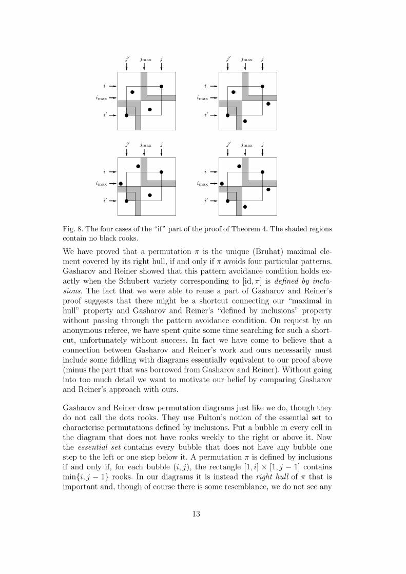
imax-

jmax

?

i -

j

?

i′ -

j′

?

imax-

jmax

?

i -

j

?

i′ -

j′

?

imax-

jmax

?

i -

j

?

i′ -

j′

?

imax-

jmax

?

i -

j

?

i′ -

j′

?

Fig. 8. The four cases of the “if” part of the proof of Theorem 4. The shaded regionscontain no black rooks.

We have proved that a permutation π is the unique (Bruhat) maximal ele-ment covered by its right hull, if and only if π avoids four particular patterns.Gasharov and Reiner showed that this pattern avoidance condition holds ex-actly when the Schubert variety corresponding to [id, π] is defined by inclu-sions. The fact that we were able to reuse a part of Gasharov and Reiner’sproof suggests that there might be a shortcut connecting our “maximal inhull” property and Gasharov and Reiner’s “defined by inclusions” propertywithout passing through the pattern avoidance condition. On request by ananonymous referee, we have spent quite some time searching for such a short-cut, unfortunately without success. In fact we have come to believe that aconnection between Gasharov and Reiner’s work and ours necessarily mustinclude some fiddling with diagrams essentially equivalent to our proof above(minus the part that was borrowed from Gasharov and Reiner). Without goinginto too much detail we want to motivate our belief by comparing Gasharovand Reiner’s approach with ours.

Gasharov and Reiner draw permutation diagrams just like we do, though theydo not call the dots rooks. They use Fulton’s notion of the essential set tocharacterise permutations defined by inclusions. Put a bubble in every cell inthe diagram that does not have rooks weekly to the right or above it. Nowthe essential set contains every bubble that does not have any bubble onestep to the left or one step below it. A permutation π is defined by inclusionsif and only if, for each bubble (i, j), the rectangle [1, i] × [1, j − 1] containsmin{i, j − 1} rooks. In our diagrams it is instead the right hull of π that isimportant and, though of course there is some resemblance, we do not see any

13

obvious connection between Gasharov and Reiner’s rectangle condition for theessential set and the right hull of the permutation.

5 Poincare polynomials of An

In this section we apply Theorem 4 to the lower Bruhat interval [id, w] of thesymmetric group An where w is the maximal minimal coset representativew = maxAS\{sk}

n . In the end we obtain the simple formula of Theorem 8.

Let Jm,n denote the m×n matrix with all entries equal to one. The followingis a q-analogue of the corollary to Theorem 1 in [5].

Proposition 14 Let A and B be zero-one matrices of sizes m×m and n×n,respectively. The block matrix

B#Adef=

B Jn,m

Jm,n A

has the (m + n)th q-rook number

RB#Am+n (q) =

min(m,n)∑

i=0

RAm−i(q) RB

n−i(q) [i]!2q q−i2 .

PROOF. It is easy to see that each configuration π of m + n rooks on B#Ais chosen uniquely by the following procedure:

• First, choose a nonnegative integer i.• Then choose a configuration A of m − i rooks on A and a configuration B

of n − i rooks on B. Together A and B form a configuration of m + n − 2irooks on

(

B 00 A

)

.• Let X be the i× i submatrix consisting of the remaining free one-entries of

(

0 Jn,m

0 0

)

, i.e. the one-entries whose row and column have no rook in A orB. Similarly, let Y be the i × i submatrix consisting of the remaining freeone-entries of

(

0 0Jm,n 0

)

. Now choose a configuration X of i rooks on X anda configuration Y of i rooks on Y .

Let Inv(π) be the set of inversions of π, i.e. pairs (r, r′) of rooks such that r isstrictly north-east of r′. The number invA(A) counts the cells in A which haveno rooks to the right or below. This equals the number of inversions (r, r′)such that r belongs to A or Jn,m and r′ belongs to A or Jm,n:

invA(A) = |{(r, r′) ∈ Inv(π) : r ∈(

0 Jn,m

0 A

)

, r′ ∈(

0 0Jm,n A

)

}|.

14

Similarly, invB (B) counts the cells in B which have no rooks to the left orabove, so

invB (B) = |{(r, r′) ∈ Inv(π) : r ∈(

B Jn,m

0 0

)

, r′ ∈(

B 0Jm,n 0

)

}|.

We also have

invX(X ) = |{(r, r′) ∈ Inv(π) : r, r′ ∈(

0 0Jm,n 0

)

}|.

and

invY (Y) = |{(r, r′) ∈ Inv(π) : r, r′ ∈(

0 Jn,m

0 0

)

}|.

Putting the above equations together yields

invA(A) + invB (B) + invX(X ) + invY (Y)

= inv(π) + |{(r, r′) ∈ Inv(π) : r ∈(

0 Jn,m

0 0

)

, r′ ∈(

0 0Jm,n 0

)

}| (2)

= inv(π) + i2

where inv(π) = |Inv(π)|. Now we exponentiate and sum over all permutationsπ which can be constructed by the procedure above:

∑

π

qinv(π) =min(m,n)

∑

i=0

q−i2RAm−i(q)R

B

n−i(q)RXi (q)RY

i (q).

By Corollary 3, RXi (q) = RY

i (q) = [i]!q. 2

Proof of Theorem 8 The Coxeter system (An−1, S = {s1, s2, . . . , sn−1})(see Figure 4) is isomorphic to the symmetric group Sn with the adjacenttranspositions si = (i ↔ i + 1) as generators. A permutation w ∈ Sn can berepresented by a rook configuration on Jn,n with n rooks, so that w(i) = jprecisely if there is a rook in the cell (i, j).

Let w be the maximal element in AS\{sk}n−1 , i.e.

(

w(1), w(2), . . . , w(n))

=(

n −

k + 1, n − k + 2, . . . , n, 1, 2, . . . , n − k)

. Using the triangle matrix Tn defined

in the end of Section 2, we can write HR(w) = (T

n−k#Tk)l and hence

Poin[id,w](q) = R(T

n−k#Tk)l

n (q) = q(n2)R

T

n−k#Tk

n (1/q)

which by Proposition 14 equals

q(n2)

min(k,n−k)∑

i=0

RTn−k

n−k−i(1/q)RTkk−i(1/q)[i]!

21/qq

i2.

15

Using Eq. (1) we obtain

P (q) = q(n2)

min(k,n−k)∑

i=0

q−(n−k2 )Sn−k+1,i+1(1/q)q

−(k2)Sk+1,i+1(1/q)[i]!

21/qq

i2 .

Since [i]!1/q = [i]!q · q−(i

2) we are done. 2

6 The number of elements in some lower intervals of An

For a general minimal coset representative w ∈ AS\{sk}n−1 , it seems very hard

to compute the complete Poincare polynomial. In this section we will solvethe easier problem to determine Poin[id,w](1), i.e. the number of elements of[id, w]. We obtain a recurrence relation that allows us to count the elements in

polynomial time. In the special case when w is the maximal element in AS\{sk}n−1

this method results in a formula different from what we get if we put q = 1in Theorem 8. From this, rather unexpectedly, we obtain a new proof of anidentity of Stirling numbers due to Arakawa and Kaneko [1].

The set of minimal coset representatives AS\{sk}n−1 consists of the permutations

w ∈ Sn with w(1) < w(2) < · · · < w(k) and w(k+1) < w(k+2) < · · · < w(n).Such a permutation clearly avoids the patterns in Corollary 5 so the numberof elements in the Bruhat interval [id, w] is given by the nth rook numberRHR(w)

n . Fortunately HR(w) has a simple structure. If w(k) < n then, as canbe seen in Figure 9,

(

w(w(k) + 1), w(w(k) + 2), . . . , w(n))

=(

n − w(k) + 1, n − w(k) + 2, . . . , n)

,

so the interval [id, w] is isomorphic (as a poset) to the interval [id, w′] inAw(k)−1, where w′(i) = w(i) for i = 1, 2, . . . , w(k). Thus we may assumethat w(k) = n. Then HR(w) = λ/µ, where λ and µ are right-aligned Ferrersmatrices with row lengths

ri(λ) =

n if 1 ≤ i ≤ k,

n − w(i) + 1 if k + 1 ≤ i ≤ n,

ri(µ) =

n − w(i) if 1 ≤ i ≤ k,

0 if k + 1 ≤ i ≤ n.

For 1 ≤ i ≤ k, let Pi be the n × n zero-one matrix with ones in the cells(i, 1), (i, 2), . . . , (i, w(i)). It is easy to see that a rook configuration with nrooks is covered by λ/µ if and only if it is covered by λ and not by any λ−Pi.

16

Fig. 9. If w(k) < n as in the left example, we may instead study the smaller exampleto the right. They have isomorphic lower intervals.

Thus, by the principle of inclusion-exclusion we get

Rλ/µn =

∑

I⊆[k]

(−1)|I|Rλ−∪i∈IPin .

By a suitable permutation of the rows, the matrix λ − ∪i∈IPi can be trans-formed to a Ferrers matrix ν with column lengths

cj(ν) = cj(λ) − |{i ∈ I : w(i) ≥ j}| = cj(λ) − |w(I) ∩ [j, n]|,

where w(I) = {w(i) : i ∈ I} denotes the image of I under w. Theorem 1with x = 0 gives

Rλ/µn = Rλ/µ

n (0) =∑

J⊆w([k])

(−1)|J |n

∏

j=1

(cj(λ) − |J ∩ [j, n]| − j + 1).

As we will see in a moment, this expression can be computed efficiently bydynamic programming.

For 1 ≤ a ≤ n and 0 ≤ b ≤ n, let

f(a, b) =∑

J∈(w([k])∩[a,n]

b )

n∏

j=a

(cj(λ) − |J ∩ [j, n]| − j + 1)

where(

w([k])∩[a,n]b

)

denotes the set of subsets of w([k]) ∩ [a, n] of size b. Also

put f(a, b) = 0 if b < 0. It is straightforward to verify the following recurrencerelation:

f(a, b) =(

ca(λ)−a−b+1)

f(a+1, b) if n > a 6∈ w([k]),

f(a, b) =(

ca(λ)−a−b+1)(

f(a+1, b) + f(a+1, b−1))

if n > a ∈ w([k]),

f(n, b) = δb,0.

(3)

17

Here δb,0 is Dirac’s δ-function which is 1 if b = 0 and 0 otherwise. Since

Rλ/µn =

k∑

b=0

(−1)bf(1, b) (4)

the number of elements in [id, w] is computable in polynomial time.

A special application of the method above admits us to prove our by-productTheorem 10.

Proof of Theorem 10 Consider the case when w is the maximal element inA

S\{sk}n−1 , i.e.

(

w(1), w(2), . . . , w(n))

=(

n−k+1, n−k+2, . . . , n, 1, 2, . . . , n−k)

.

Then ca(λ) = k + a if a ≤ n − k and ca(λ) = n if a ≥ n − k + 1, so therecurrence (3) becomes

f(a, b) = (k − b + 1)f(a + 1, b) if a ≤ n − k,

f(a, b) = (n−a−b+1)(

f(a+1, b) + f(a+1, b−1))

if n−k+1 ≤ a ≤ n−1.

f(n, b) = δb,0

Iteration of the first line of the recurrence yields

f(1, b) = (k − b + 1)n−kf(n − k + 1, b). (5)

Putting g(α, β) = f(n−α+1, α−β) for 1 ≤ α ≤ k, our recurrence transformsto

g(α, β) = β ·(

g(α − 1, β) + g(α − 1, β − 1))

if 2 ≤ α ≤ k.

g(1, β) = δβ,1

We recognise this as the recurrence for β!Sα,β where Sα,β are Stirling numbersof the second kind; thus f(a, b) = (n−a−b+1)!Sn−a+1,n−a−b+1 for n−k+1 ≤a ≤ n. Combining this with Eq. (5) and plugging the result into Eq. (4), weobtain

Rλ/µn =

k∑

b=0

(−1)b(k − b + 1)n−k(k − b)!Sk,k−b

which also can be written as

(−1)kk

∑

i=0

(−1)i(i + 1)n−ki!Sk,i.

This happens to be the formula for the poly-Bernoulli number Bk−nn defined

by Kaneko [15]. 2

18

7 Type B

In this section we compute the Poincare polynomial of the lower Bruhat inter-val [id, w] in the hyperoctahedral group Bn, where w is the maximal minimalcoset representative, w = maxBS\{s0}

n .

We will represent Bn combinatorially by the set SBn

def= {π ∈ S2n : π = π}

of rotationally symmetric maximal rook configurations on J2n,2n, see [2, Ch. 8].In this representation π ≤ ρ in Bruhat order on Bn if and only if π ≤ ρ aselements of S2n ([2, Cor. 8.1.9]). The rank of π is

ℓ(π) =(

inv(π) + neg(π))

/2 (6)

where inv(π) is the usual inversion number of π as an element of S2n, and

neg(π)def= |{i ∈ [n + 1, 2n] : π(i) ≤ n}|, see [2, Ch. 8, Exercise 2].

For a zero-one matrix A of size 2n × 2n, let

RBA(q, t)def=

∑

π∈SBn ∩S(A)

qinv(π)tneg(π).

Proposition 15 Let A be a zero-one matrix of size n × n. Then

RBA#A(q, t) =n

∑

i=0

RAn−i(q

2) [i]!q2 q−i2ti.

PROOF. The proof is almost identical to the proof of Proposition 14.

When m = n, it is easy to see that the permutation π constructed by theprocedure in the proof of Proposition 14 is rotationally symmetric if and onlyif B = A and Y = X. Thus, putting m := n, B := A, Y := X = X,B := A, and Y := X into Eq. (2) and using the identity (A) = A, weobtain

2 (invA(A) + invX(X )) = inv(π) + i2.

Obviously, neg(π) = i. Exponentiation and summation over all rotationallysymmetric permutations π on A#A yields

∑

π

qinv(π)tneg(π) =n

∑

i=0

q−i2RAn−i(q

2)RXi (q2)ti.

By Corollary 3, RXi (q2) = [i]!q2 . 2

Now we are ready for the proof of Theorem 9.

19

Proof of Theorem 9 From Theorem 4 and Eq. (6) we obtain

Poin[id,w](q) =∑

u∈[id,w]

qℓ(u) = RBHR(w)(q1/2, q1/2).

It is easy to see that HR(w) = (T n #Tn)l. Hence

Poin[id,w](q) = RB(T n #Tn)l(q1/2, q1/2) = qn2

RB(T n #Tn)(q−1/2, q−1/2)

where we have used the fact that

RBAl

(q, t) = q(2n2 )tnRBA(q−1, t−1)

for any 2n × 2n zero-one matrix A. By Proposition 15 we can now compute

Poin[id,w](q) = qn2n

∑

i=0

RTnn−i(1/q)[i]!1/qq

(i2).

Using Eq. (1) and the identity [i]!1/qq(i2) = [i]!q, we finally obtain

Poin[id,w](q) = q(n+1

2 )n

∑

i=0

Sn+1,i+1(1/q)[i]!q. 2

8 Open problems

Perhaps the reason we still do not know much about the Poincare polynomialsof Bruhat intervals after several decades of research in the area is the lack ofnatural methods to attack it. We hope the framework and the tools presentedhere will make the problem more accessible, and we would like to suggest anumber of interesting open questions.

• What is the Poincare polynomial Poin[id,w](q) in the even-signed permuta-tion group Dn if w = maxDS\{s0}

n is the maximal minimal representative inthe quotient modulo a maximal parabolic subgroup isomorphic to An−1?

• What is Poin[id,w](q) in the affine group An?• Are there formulas for the generalised Eulerian polynomial

∑

v∈[id,w] td(v) or

even for the bivariate generating function∑

v∈[id,w] td(v)qℓ(v), where d(v) =

|{s ∈ S : ℓ(vs) < ℓ(v)}| is the descent number of v?• In a recent paper by Bjorner and Ekedahl [3] it is shown (for any crystallo-

graphic Coxeter group) that 0 ≤ i < j ≤ ℓ(w) − i implies fwi ≤ fw

j , wherefw

i is the qi-coefficient of Poin[id,w](q). Perhaps one can say more about theparticular Poincare polynomials discussed in the present paper. Computerexperiments support the following conjecture:

20

Conjecture 16 The Poincare polynomials of Theorem 8 and 9 are uni-modal.

• As noted by Gasharov and Reiner [11, p. 559], Ding’s partition varieties [8]correspond not only to certain Bruhat intervals of the whole group An butalso to some intervals of the quotient An/(An)J for certain parabolic sub-groups (An)J . Can something similar be done in the more general settingof skew partition varieties?

• Given a polynomial, what board (i.e. zero-one matrix), if any, has it as itsrook polynomial? In 1970 Foata and Schutzenberger [9] showed that distinctincreasing Ferrers boards have distinct rook polynomials, and in a recentpaper [18] Mitchell characterised these polynomials in terms of roots anddivisibility. What is true for skew Ferrers boards?

• Develin [7] classified the isomorphism types of lower Bruhat intervals of 312-avoiding permutations by using the connection to rook posets discoveredby Ding [8]. What are the isomorphism types of lower Bruhat intervals ofpermutations that avoid the patterns 4231, 35142, 42513, and 351624?

9 Acknowledgement

I would like to thank Torsten Ekedahl for asking a question that made mewrite this paper. Many thanks also to Anders Bjorner, Richard Stanley, AxelHultman, Stephane Launois, and an anonymous referee for valuable comments.

References

[1] T. Arakawa and M. Kaneko, On poly-Bernoulli numbers, Comment. Math.Univ. St. Pauli 48:2 (1999) 159–167.

[2] A. Bjorner and F. Brenti, Combinatorics of Coxeter Groups, Springer, 2005.

[3] A. Bjorner and T. Ekedahl, On the shape of Bruhat intervals,arXiv:math.CO/0508022.

[4] A. Bjorner and M. Wachs, Bruhat order of Coxeter groups and shellability,Adv. in Math. 43 (1982) 87–100.

[5] G.-S. Cheon, S.-G. Hwang, and S.-Z. Song, Rook polynomials to and frompermanents, Discrete Math. 264 (2003) 25–36.

[6] C. Chevalley, Sur certain groupes simples, Tohoku Math. J. 7 (1955) 14–66.

[7] M. Develin, Rook poset equivalence of Ferrers boards, Order 23 (2006) 179–195.

[8] K. Ding, Rook placements and cellular decomposition of partition varieties,Discrete Math. 170 (1997) 107–151.

21

[9] D. Foata and M.-P. Schutzenberger, On the rook polynomials of Ferrersrelations, Colloquia Math. Soc. Janos Bolyai 2:4 (1970) .

[10] A. M. Garsia and J. B. Remmel, Q-counting rook configurations and a formulaof Frobenius, J. Combin. Theory Ser. A 41 (1986) 246–275.

[11] V. Gasharov and V. Reiner, Cohomology of smooth Schubert varieties in partialflag manifolds, J. London Math. Soc. 66:2 (2002) 550–562.

[12] J. Goldman, J. T. Joichi, and D. White, Rook theory I. Rook equivalence ofFerrers boards, Proc. Amer. Math. Soc. 52 (1975) 485–492.

[13] A. Hultman, Bruhat intervals of length 4 in Weyl groups, J. Combin. TheorySer. A 102 (2003) 163–178.

[14] F. Incitti, New results on the combinatorial invariance of Kazhdan-Lusztigpolynomials, J. Algebra 309 (2007) 139–167.

[15] M. Kaneko, Poly-Bernoulli numbers, J. Theor. Nombres Bordeaux 9 (1997)221–228.

[16] S. Launois, Combinatorics of H-primes in quantum matrices, J. Combin. TheorySer. A (2006) , doi:10.1016/j.jcta.2006.06.009.

[17] L. Lovasz, Combinatorial Problems and Exercises, Elsevier Science Publishersand Akademiai Kiado, 2nd edition, 1993.

[18] A. G. Mitchell, The inverse rook problem on Ferrers boards, 2004,arXiv:math.CO/0407007.

[19] N. Reading, On the structure of Bruhat order, 2002, available online athttp://www4.ncsu.edu/~nreadin/papers/thesis.pdf.

[20] N. Reading, The cd-index of Bruhat intervals, Electron. J. Combin. 11 (2004)#R74.

[21] L. Solomon, The orders of the finite Chevalley groups, J. Algebra 3 (1966)376–393.

[22] R. Steinberg, Endomorphisms of linear algebraic groups, Mem. Amer. Math.Soc. 80 (1968) 1–108.

[23] D.-N. Verma, Mobius inversion for the Bruhat order on a Weyl group, Ann.Sci. Ecole Norm. Sup. 4 (1971) 393–398.

[24] K. Vesztergombi, Permutations with restriction of middle strength, Studia Sci.Math. Hungar 9 (1974) 181–185.

22

enumerative combinatorics related to partition shapes - diva portal

Documents