materials, methods & technologies journal of …...materials, methods & technologies issn...

Materials, Methods & Technologies

ISSN 1314-7269, Volume 10, 2016

Journal of International Scientific Publications

www.scientific-publications.net

Page 25

ELECTROMAGNETIC INDUCTION SIMULATION FOR DEFECTS DETECTION:

INVOLVED VARIABLES AND ITS EFFECTS

Fernandez-Perez Nora, Gamallo-Ponte Pablo

Inspiralia Tecnologias Avanzadas SL, Calle Estrada 10-B, 28034 Madrid, Spain

Abstract

This paper describes the study carried out to identify the involved parameters and its effects, in

surface defect detection of metallic pieces through electromagnetic induction. The technique is known

by Induction Thermography, and the detection under the produced electrical field occurs due to the

induced current concentration on the edges of the defects that can be finally detected by a

thermographic camera. To aid in the analysis of the problem, involved physics as well as the related

parameters, a simulation method was developed. A coupled electromagnetic and thermal finite

element model was created with the software ANSYS. Through this method the influence of the

different variables involved, such as geometry or configuration (dimensions, shape, location,

orientation, etc.) and the electrical or input parameters, as well as the time dependency was assessed

in the obtained simulation results. In fact the evidence about the detection process effectiveness and

efficiency was studied, based on data such as induced current density concentration, heating

uniformity, electrical power required, cycle time, etc. Thus the goal of this paper is to find out the

influence of the different configurations and variables involved, to finally provide a system with the

best result in terms of reduced energy and time consumption. This model is the result of a previously

validated work (ref), and thus it is a consistent and reliable tool for induction heating analyses and for

the optimization of surface crack detection processes based on Induction thermography. It will highly

reduce time and economic investments, prior to the physical construction and tests of the system.

Key words: electromagnetic induction, induction thermography, electro-thermal modeling, numerical

simulation

Introduction

Computational methods are widely used for simulations in different engineering fields: mechanical,

thermal, electrical, etc. However, the use of simulation tools for the analysis and design of systems

involving electromagnetics (alone or coupled with other physics) is still reduced in industrial

applications, mainly due to the following reasons: the complexity of simulating coupled non-linear and

three-dimensional problems and the need of high performance computers. However in the last years

much effort has being concentrated on the study and development of simulation methods for solving

electromagnetic problems (1) (2). The reason might lie in the increasingly use of electromagnetic

systems in the industry, in particular for induction heating applications. In fact, induction heating

provides many advantages compared to traditional heating processes (for instance gas furnaces),

mainly: a fast heating rate, well-defined heating locations, good reproducibility and low energy

consumption, reduction of start-up and shutdown timing, low equipment and labour cost and low

carbon footprint (3).

Electromagnetic Induction heating is based on the phenomenon by which an alternative current

flowing through a coil induces a magnetic field and the subsequent eddy currents on an electrically

conductive target part (workpiece). These eddy currents heat up the target workpiece due to the Joule

effect. Thus, the heating pattern will be very closely related to the geometry of the target and the path

of the coil, but also to other issues such as the skin effect (penetration of the currents below the piece

surface), proximity and slot effects intrinsically related to the induction electromagnetic phenomena

(4). In fact, these effects are those typically causing the non-uniform heating of magnetic pieces

induced through conventional conductors. Thus, no uniform currents are induced through the

workpiece and the heat generation is concentrated on the surface.


ISSN 1314-7269, Volume 10, 2016



6

This paper explores the heating and temperature distribution caused by an induction system through

the Finite Element Method (FEM), the different parameters involved and its influence. The goal is to

optimize the surface defect inspection of the Induction Thermography system and thus to find the

optimum parameters for which the induced current concentration will be the highest, avoiding at the

same time, an excessive heating of the piece (the defined temperature limit is 60°C). The final goal

will be to assure a proper defect detection at the minimum process time as possible and through the

most efficient way.

This work consists of two parts. In the first part, a sensibility analysis was carried out comprising the

study of the influence of the electrical and associated generator parameters (power, frequency, etc.). In

the second part of this work, the geometrical parameters and its effects on defects detection are

studied: the coil-piece disposition, coil geometry (path, dimensions and location), as well as the

influence of the defect shape on the detection.

For this purpose a numerical method for the simulation of induction heating systems was implemented

in the FEM software ANSYS® APDL. The reliability and accuracy of the simulation method, which

couples electromagnetism and heat transfer, was proven through previous experimental test (5). Due to

the proven reliability of this tool, it was used to analyse the different variables that will influence on

the resulting induced current pattern and its efficiency.

A parametric model was developed to study the behaviour of the different cases in a more automatic

way. The obtained temperature distributions provided information about the suitability and

performance of the different variables involved and thus about the most proper system configurations,

by considering: first the maximum temperature each component can stand for security purposes, the

defect detection capability and finally the efficiency or cycle times achieved.

Mathematical model and simulation method

In this section the equations for modelling the heat induction process are introduced; on the one hand,

the electromagnetic and on the other the heat transfer equations are presented. The simulation method

implemented is based on the numerical solution of these mathematical equations by means of the finite

element method.

Electromagnetic model

The electromagnetic fields in matter obey the so-called macroscopic Maxwell’s equations. These

equations relate the electromagnetic fields: electric field , the displacement field , the magnetic

flux density , the magnetic field intensity , the free current density , and the free electric charge

density . The free charge and current refer to those not associated with matter (dielectric and/or

magnetic materials).

For general time-varying electromagnetic fields, the Maxwell equations in differential form can be

written as (6):

Ampere’s law (with Maxwell addition)

Faraday’s law

Gauss’s law for magnetism

Gauss’s law

These equations have to be complemented with the continuity equation (charge conservation)

and the corresponding constitutive equations of each material:


ISSN 1314-7269, Volume 10, 2016



Page 27

( ) ( )

The materials analysed in this work can be considered as linear, isotropic and homogeneous

where is the vacuum permittivity and the vacuum permeability and and the corresponding

material relative permittivity and permeability.

For the electrical conductive materials holds

, Ohm’s law

where σ is the material electric conductivity.

Since alternating (harmonic) input currents (voltages) are considered, under the previous assumptions,

the steady-state harmonic fields will have the following form in complex notation:

( ) [ ( )]

where represents time, is the position, is the angular frequency of the input current, the

imaginary unit number and ( )is the complex amplitude of the field.

The induction systems used in industry for heating process work in the so-called low-frequency

regime. For low-frequency, the term in Ampere’s law including the electric displacement can be

neglected and the Maxwell’s equations reduce to the so-called harmonic eddy current model:

The current set to flow along the inductor coil is related to the current density through the equation

∫

where is the coil cross section.

Finite Element Model. Mesh and skin effect

This set of equations can be discretized with the Finite Element Model, as implemented in the

ANSYS® Emag software (7) (8), to solve them numerically. The outputs of these electromagnetic

simulations are the generated electromagnetic fields and the induced eddy currents.

In order to ensure a good accuracy of the FEM simulations, it is crucial that the finite element mesh is

characterized by a refined element size on the surface of the workpiece to represent properly the

aforementioned skin effect. This is a very significant effect to take into account to achieve a reliable

model, since the eddy currents will be concentrated on the surface of the part and thus, the FEM

should include more than one element within the skin depth . Fortunately, the thickness of the skin

depth can be estimated accurately from the following relation:

√

On the other hand, in order to represent in the FEM model the ‘unbounded’ air surrounding the

system, a finite size air box enclosing the workpiece and the inductor with suitable boundary

conditions (magnetic flux tangential to its faces) was considered.


ISSN 1314-7269, Volume 10, 2016



Page 28

With regard to the coil, it is treated as a source conductor with a given current (provided by the

generator) and hence a current intensity is introduced from one end of the coil and a ground (zero)

voltage is set on the other end.

Since the electromagnetic transient period, previous to the steady-state harmonic regime, is very short

in time and it can be neglected. Thus the initial conditions have no influence and therefore are not

required in the numerical model.

Heat transfer model

The electromagnetic model must be coupled with the heat transfer problem, to study the thermal

effects of the induction phenomena. The following equations will guide the thermal behaviour, which

varies depending on the element location: inside de model (conduction effects) or in the exterior

surface (which accounts for conduction, radiation and convection effects).

, condition inside

(

) ( ), condition on the

surface

The heat generated in the materials by the electric currents due to the Joule effect is included as a heat

source in the heat conductive equation:

( )

| |

where is the temperature and and the material density, specific heat and thermal conductivity,

respectively.

The boundary conditions of the heat transfer problem consider the Newton’s law of cooling with an

effective heat transfer coefficient in the exterior surfaces of the pieces, to account for heat

losses/gains from convection and radiation (linearized) with the surrounding media (air in our

study).

( )

The numerical solution of the thermal problem is performed by means of the Finite Element

discretization (9) of the above heat transfer equation as implemented in ANSYS® Mechanical APDL.

Assuming that the variation of the electromagnetic properties ( T , T , ) with temperature is

negligible, the coupling between the electromagnetic and thermal models reduces to a one-way, that is,

the harmonic EM problem is solved first to compute the heat source produced by the Joule effect and

this heat will be the input in the transient heat transfer problem.

Simulation Model

In this section the developed simulation model is described, including the geometry, materials

employed and boundary conditions. The geometry is described for the model that will be used as a

reference case.

Geometry

The geometry of the analysis comprises a copper coil and a steel plate (Figure 1), as well as the

surrounding air. A crack was also represented on the plate transversely located to the coil. The air

body containing the coil and plate was included to account for the magnetic field enclosure.


ISSN 1314-7269, Volume 10, 2016



Page 29

Figure 1. Simulation model (left) and dimensions of the reference model (right)

As previously mentioned a current will be set on the coil entrance, which simulates a system

connected to a power-supply and carrying an alternating electric current. This current will produce a

rapidly oscillating magnetic field which will generate the corresponding eddy currents (depending on

the input values) in the plate. Finally in the thermal transient simulations temperature patterns

generated due to the Joule effect will be observed.

Materials

The material properties required for the simulation are presented here, the electromagnetic properties

on the one hand and thermal properties on the other.

Electromagnetic properties

Magnetic permeability

Several parameters may be used to describe the magnetic properties of solids. One of those is the ratio

of permeability in a material to the permeability in vacuum:

where µr is called the relative permeability, unitless. The permeability or relative permeability of a

material is a measure of the degree to which the material can be magnetized, or the ability by which a

B field can be induced in the presence of an external H field. This is one of the most important

material properties that may influence on the electromagnetic simulation, mainly that corresponding to

the plate. In fact the relative permeability will be closely related to the skin depth of the system (as

shown in the skin effect equation mentioned above). The magnetic permeability is also highly

dependent on the hysteresis curve. For this study it was considered that the permeability will not

achieve the saturation environment that may be given at high magnetic field values (A/m).

Electrical conductivity

The electrical conductivity of the material will be as well an important input for the electromagnetic

simulation. The electrical conductivity will provide the ability of the material to conduct the electrical

current. The SI units are S/m (siemens/m). The inverse is the electric resistivity which units are Ω·m.

Thermal properties

The physical properties of the materials implied on the heat transfer problem are density (kg/m3), heat

capacity (J/KgK) and thermal conductivity (W/mK). Those will be defined for each material on the

following section.


ISSN 1314-7269, Volume 10, 2016



Page 30

Table 1. Material properties

ρ

(kg/m3)

Cp

(J/kg K)

K

(W/m K)

Elec.Res

(ohm m)

µrel

AIR 1.2 1004 0.0257 - 1

STEEL 7850 486 51.9 1.17e-7

2000-5000

COPPER 8300 385 401 1.7e-8

1

Meshing

Electromagnetic studies require a fine mesh, especially on the target surface where the eddy current

will mostly take place, i.e. the skin depth. Thus a very fine mesh is required on the plate surface to

account for the eddy current and the heat source generated by those. At least two elements have to be

introduced within the skin depth (3.8µm-5.07µm). So finally a very fine mesh with seven layers

inflation was used to account for these effects (Figure 2), which dimension will also depend on the

frequency value introduced.

Figure 2. Coil and plate mesh (left) and detail of the surface refined mesh in the crack (right)

Boundary conditions

The Electromagnetic problem was solved with a harmonic study, with the different settings for each

case. The conditions that were imposed over the electromagnetic model are:

- A magnetic flux boundary condition to constraint the direction of the magnetic flux. By default,

this feature constraints the flux to be tangential to all exterior faces. This flux parallel condition

was applied to exterior faces of the air solid, to contain the magnetic flux inside the simulation

domain.

- The coil is the conductor source and thus the current was set on the inlet side of the coil. A zero

ground voltage was set on the other end.

In a first run of the model, the impedance Z of the coil can be determined. Once Z was computed, the

current was set again to obtain the desired power on the system. In the heat transient problem the

boundary and initial conditions are the following:

- Initial ambient temperature was set to 20°C

- Adiabatic conditions were set for the coil and plate (No convection either radiation was considered

due to the reduced time pulse at which it will run).

- The heat source obtained from the electromagnetic model was applied to the coil and plate.


ISSN 1314-7269, Volume 10, 2016



Page 31

Case studies

In order to study the effects of the different variables various analyses were performed based on the

different case studies with the defined range of values (Table 2). Within the electrical parameters the

frequency, power and material properties such as magnetic permeability of steel were studied.

Regarding the geometry and its configuration, the relative position between the coil and crack, the

orientation, distance and displacement between those was observed. The crack dimension and type

were also studied to check the detection capability of the system. The results were analyzed to see how

those input values affect on the current density and the final map of temperatures on the plate’s surface

and the crack. The different time steps at which those temperatures were obtained are also shown. The

most significant values for the case studies comprise the following value range, which are also based

also on the selected generator capability (ref).

Table 2. Studied parameters

Parameter Value

Frequency 100 – 400 KHz

Power 1 – 5 Kw

Distance coil - plate 5 – 7 mm

Position coil – crack Aligned, 90º

Crack dimensions 1x1x1 - 25x1x2 mm

Magnetic permeability 2000-5000

Sensibility analysis. Electrical parameters effects

In this section the sensibility analysis regarding the effect of the different electrical parameters:

frequency, power and material permeability is presented. First the electromagnetic induced current and

the thermal transfer on the piece was studied for the reference case (Case1), in order to have a further

comprehension of the physic and its effects. Then the comparison of the following case studies with

the reference case is presented. Thus the goal of this sensibility analysis is based on the following

cases and study:

- CASE 1: Reference case

- CASE 2: Power increase (current)

- CASE 3: Frequency increase

- CASE 4: Magnetic permeability of steel increase

Electromagnetic Induction current study and thermal transfer

Inputs

In this study the coil is centered on the plate, with a distance from the plate of 5 mm, and the crack

perpendicular to the coil. The input parameter values and crack characteristics are presented here:


ISSN 1314-7269, Volume 10, 2016



Page 32

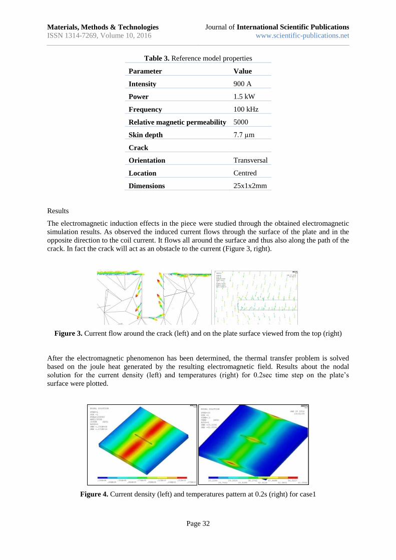
Table 3. Reference model properties

Parameter Value

Intensity 900 A

Power 1.5 kW

Frequency 100 kHz

Relative magnetic permeability 5000

Skin depth 7.7 µm

Crack

Orientation Transversal

Location Centred

Dimensions 25x1x2mm

Results

The electromagnetic induction effects in the piece were studied through the obtained electromagnetic

simulation results. As observed the induced current flows through the surface of the plate and in the

opposite direction to the coil current. It flows all around the surface and thus also along the path of the

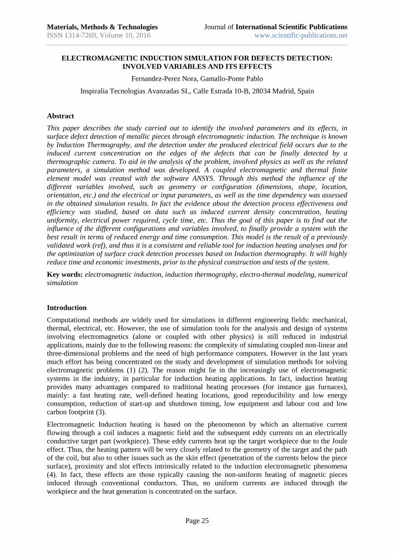
crack. In fact the crack will act as an obstacle to the current (Figure 3, right).

Figure 3. Current flow around the crack (left) and on the plate surface viewed from the top (right)

After the electromagnetic phenomenon has been determined, the thermal transfer problem is solved

based on the joule heat generated by the resulting electromagnetic field. Results about the nodal

solution for the current density (left) and temperatures (right) for 0.2sec time step on the plate’s

surface were plotted.

Figure 4. Current density (left) and temperatures pattern at 0.2s (right) for case1


ISSN 1314-7269, Volume 10, 2016



Page 33

As mentioned current densities (Figure 4, left) are higher on the corners of the cracks. When these

values are translated to temperatures (Figure 4, right) more visible results can be observed. Maximum

temperatures are found on the crack and plate border as expected (due to the border effect mentioned),

with maximum values of 61°C.

Figure 5. Zoom of the temperature pattern on crack

From these temperature pattern results, the need to plot the thermal gradient values are observed.

These high temperature changes on the borders compared to the surroundings can be given by the

thermal change per unit length of the plate.

Figure 6. Thermal gradient at 0.2s of case1

In these spatial thermal gradients the crack is highly emphasized with higher values than those

obtained on the plate border. Maximum values of 16 K/mm were obtained in the crack. This will be in

fact one of the most important results obtained from the simulation, i.e. the fact that the thermal

gradient values will highlight the existing crack.

The goal of the following study is therefore to verify this assumption on every kind of crack geometry,

orientation, etc. and define the range of electrical parameters for which this statement is present.

Case studies. characteristics and results

In this section the results of the performed case studies are shown. First the input parameters of each

case are presented.

Inputs


ISSN 1314-7269, Volume 10, 2016



Page 34

Table 4. Case 2: Intensity increase

Parameter Value

Intensity 1800 A

Power 6 kW

Frequency 100 kHz

Relative magnetic perm. 5000

Skin depth 7.7 µm

Distance Coil-Plate 5 mm

Crack:


Location Centered

Dimensions 25x1x2mm

Table 5. Case 3: Frequency increase

Parameter Value

Intensity 900 A

Power 4.6 kW

Frequency 400 kHz


Skin depth 3.8 µm


Crack:


Location Centered

Dimensions 25x1x2mm

Table 6. Case 4: Magnetic permeability

Parameter Value

Intensity 900 A

Power 1.5 kW

Frequency 100 kHz


Skin depth 7.7 µm


Crack:



ISSN 1314-7269, Volume 10, 2016



Page 35

Location Centered

Dimensions 25x1x2mm

In case 3 the increased frequency caused the increase on the power consumed by the system, from

1.5kW to 4.6kW. At the same time the skin depth was also decreased due to the increased frequency.

Results

In the following pictures the current density and temperature patterns at 0.2s are presented.

Table 7. Current density (left) and temperatures pattern at 0.2s (right)

CASE

Nº

Current density Temperatures Max.

Temp

1

61°C

2

184°C

3

155°C


ISSN 1314-7269, Volume 10, 2016



Page 36

4

51°C

Table 7, The temperature pattern (right) show that the maximum temperature occurs on the crack and

the plate border. As it could be anticipated, much higher temperatures are found high intensities and

input power (case 2 and 3), compared to the reference case (case 1).

In the following picture the thermal gradient plot at 0.2s is shown for all the cases.

Table 8. Thermal gradient results of the case studies

CASE Nº Thermal Gradient Max. Thermal gradient

1

16 K/mm

2

105K/mm

3

82 K/mm


ISSN 1314-7269, Volume 10, 2016



Page 37

4

18 K/mm

Maximum values of thermal gradients are always visible on the crack. In fact an important conclusion

from the thermal gradient results is that the maximum values are always found on the crack and not on

the borders.

In addition the electrical parameter study shows that the best performance in terms of detection

reliability is the case with the increased frequency. It provides more obvious crack recognition, due to

the higher thermal gradient encountered and at the same time not as high temperatures as when current

was increased to the maximum, which in fact is out of the scope of the induction thermography.

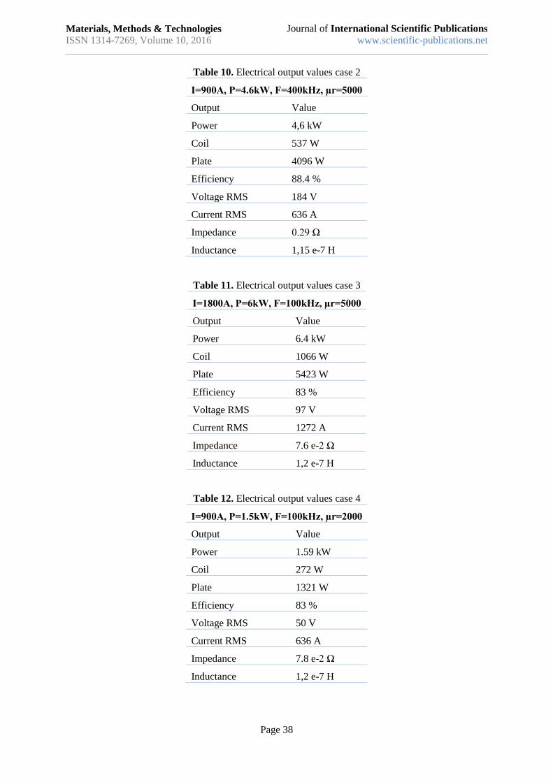
The electrical outputs are also shown in the following section. The main value that is important to see

from these results is the efficiency obtained in each case. This value corresponds to the ratio of heat

gained by the plate to the power introduced. This will be meaningful once the crack has been detected

and thus when the optimum electrical parameters have to be selected the first condition will be a clear

detection of the crack and then that which provides an improved efficiency of the system.

Within the presented case studies the highest efficiency was found on that in which the frequency was

increased to the maximum (Table 10), obtaining and efficiency of 88.4%. This is higher than the case

in which the current was increased (Table 11), 83%. This goes related to the fact that increasing the

frequency will generate a smaller skin depth and thus the current will be forced to flow through a

smaller depth, which will be translated into a higher current concentration and thus higher

temperatures.

In the case4 in which the permeability was decreased, similar results are obtained compared to the

reference model.

Table 9. Electrical output values case 1

I=900A, P=1.5kW, F=100kHz, µr=5000

Output Value

Power 1,56 kW

Coil 267 W

Plate 1293 W

Efficiency 83 %

Voltage RMS 49 V

Current RMS 636 A

Impedance 7,7e-2 Ω

Inductance 1,2e-7 H


ISSN 1314-7269, Volume 10, 2016



Page 38


I=900A, P=4.6kW, F=400kHz, µr=5000

Output Value

Power 4,6 kW

Coil 537 W

Plate 4096 W

Efficiency 88.4 %

Voltage RMS 184 V

Current RMS 636 A

Impedance 0.29 Ω

Inductance 1,15 e-7 H


I=1800A, P=6kW, F=100kHz, µr=5000

Output Value

Power 6.4 kW

Coil 1066 W

Plate 5423 W

Efficiency 83 %

Voltage RMS 97 V

Current RMS 1272 A

Impedance 7.6 e-2 Ω



I=900A, P=1.5kW, F=100kHz, µr=2000

Output Value

Power 1.59 kW

Coil 272 W

Plate 1321 W

Efficiency 83 %

Voltage RMS 50 V

Current RMS 636 A

Impedance 7.8 e-2 Ω



ISSN 1314-7269, Volume 10, 2016



Page 39

Geometric analysis

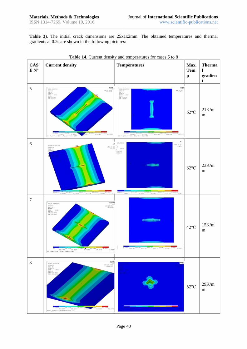
The influence of the geometry in the detection process is presented in this section, which includes the

shift of the coil from the plate surface, the orientation, the displacement from the centre, crack

dimensions and shape.

Figure 7. Case studies related to the position and orientation of the crack-current

The case studies comprise the following analysis:

- CASE 5: Orientation of the coil with respect to the crack. Aligned

- CASE 6: Displaced from the plate’s centre 5mm

- CASE 7: Distance coil-plate increased to 7mm

- CASE 8: Crack size changed to the minimum dimension of 1x1x1mm (min. accepted critical size)

Table 13. Case studies of the different geometries

Case 5 Case 6

Case 7 Case 8

In these case studies the same electrical inputs as for the reference case were introduced (


ISSN 1314-7269, Volume 10, 2016



Page 40

Table 3). The initial crack dimensions are 25x1x2mm. The obtained temperatures and thermal

gradients at 0.2s are shown in the following pictures:

Table 14. Current density and temperatures for cases 5 to 8

CAS

E Nº

Current density Temperatures Max.

Tem

p

Therma

l

gradien

t

5

62°C 21K/m

m

6

62°C 23K/m

m

7

42°C 15K/m

m

8

62°C 29K/m

m


ISSN 1314-7269, Volume 10, 2016



Page 41

Again the maximum thermal gradient values are found on the tips. These values are very similar to

those obtained in the reference case (Case 1). In case 7, due to the shift of the coil from the plate,

obtained values are lower (patterns are identical). In case 8 the lower dimensions of the crack provide

a higher concentration on the crack.

Time influence of detection results

In this section the heat diffusion along time is shown. Temperature and gradient maps for the reference

case (case 1) and the most significant case ( case 3, with 400 Hz) are shown. The following sequence

of images comprises the nodal solution temperature at 0.05, 0.1 and 0.2 seconds, for the reference

case.

Figure 8. Temperature and thermal gradient at 0.05 sec (Tmax=35°C)

Figure 9. Temperature and thermal gradient at 0.1s (Tmax=42°C)

Figure 10. Temperature and thermal gradient at 0.2s. (Tmax=61°C)


ISSN 1314-7269, Volume 10, 2016



Page 42

In these time steps the temperature increases as the time increase and the maximum thermal gradient

(16 k/mm) is equal for the three of them. The difference stays on the fact that the heat diffusion starts

and thus the thermal concentration may be spread as the time goes by. In the following sequence of

images the nodal solution of the thermal gradient at 0.05, 0.1 and 0.2 seconds, for the case in which a

current with a frequency of 400kHz was introduced (case 3).

Figure 11. Time: 0.05 seconds. Tmax=80°



The maximum thermal gradient in all those cases was 82K/mm. Again the difference is that the heat

diffusion starts and thus the thermal gradient may be spread as the time goes by. From this study a

very important result is concluded in which it can be seen that high frequency could be used for small

time steps, due to the fact that it does not achieve very high temperatures, as desired.


ISSN 1314-7269, Volume 10, 2016



Page 43

Conclusions

Important conclusions were obtained from the herein presented study. In general terms temperature

maps show the maximum heat on the tips and colder flanks. However and this is one of the most

important conclusions obtained from simulation; the crack will show up more clearly on thermal

gradient solutions than in thermal maps images. Moreover, the border effect is eliminated on the

thermal gradient results, showing its maximum on the crack tips. The thermal gradient plot will

highlight the crack onto the surface at every time step. However small time step will be preferable,

before the heat diffusion starts.

In the cases in which permeability (2000 – 5000) was changed not significant changes are observed,

very similar values were obtained. However an additional study should be required to see how the fact

of being on the non linear area of the Hysteresis curve will affect to the obtained results.

When intensity or frequency was increased significant changes were found (Table 10 and Table 11).

Higher current density concentration and higher temperatures are found, which are higher than those

expected by the allowd temperatures (70C). However lower temperature can be found at smaller time

step and in addition, higher evidence of the crack will be found on the thermal gradient pattern.

When the frequency was increased to its maximum (400kHz for the selected generator) the most

evident crack detection results were obtained and moreover the use of power was found to be the most

efficient. This goes related to the fact that the frequency increase will generate a smaller skin depth

and thus the current will be forced to flow through a smaller depth, which will be translated into a

higher current concentration and thus higher thermal gradient. However very high temperatures were

obtained at 0.2s, but lower can be found at smaller time step (around 80C at 0.05s).

Form the time influence study study it was observed that temperature changes very quickly along very

small time steps and that the heat diffuses very rapidly.

Acknowledgments

This work was carried out in the scope of the EU FP7 TRAINWHEELS project (grant agreement no:

ID 603410).

References

1. Bermudez de Castro, Alfredo, Gomez, Dolores and Salgado, Pilar. Mathematical models and

numerical simulation in electromagnetism. s.l. : Springer, 2014.

2. Large-Scale Electromagnetic Computation for Modeling and Applications. Qing Huo Liu, Lijun

Jiang, Weng Cho Chiew. 2, s.l. : IEEE, 2013, IEEE, Vol. 101.

3. Davies, E.J. Conduction and Induction Heating. London : Peregrinus, 1990.

4. Rudney, Valery, et al., et al. Hand book of Induction Heating (Manufacturing Engineering and

Materialas processing). 2003.

5. Perez, Nora Fernandez. Validation of an electromagnetic induction simulation for defects

detection: A quasi-static model for an automated inspection system. 2015.

6. Cessenat, M. Mathematical methods in Electromagnetism. s.l. : World Scientific, 1996.

7. ANSYS Inc. Low Frequency Electromagnetic Analysis. 2009.

8. —. Coupled field analysis guide. 2009.

9. Zienkiewicz, O.C. and Taylor, R. L. The Finite Element Method. s.l. : Butterworth-Heinemann,

2000.

10. A. Bossavit. Computational Electromagnetism. San Diego CA : Academis Press, 1998.


ISSN 1314-7269, Volume 10, 2016



Page 44

11. D1.1, Inspiralia. Deliverable 1.1. Report on the geometrical and physical characterization of

wheel-axles systems and the surface cracks to be detected. Madrid : s.n., 2014.

12. D2.1, Inspiralia. Deliverable 2.1. Computation of thermal maps for different configurations if

induction system and cracks. 2014.

13. Thermal and magnetic field analysis of induction heating problems. Hiroki Kawaguchi, Masato

Enokizono, Takashi Todaka. 193–198, Oita, Japan : s.n., (2005), Vol. Journal of Materials

Processing Technology 161 .

14. Defect characterisation based on heat diffusion using induction thermography testing. Yunze He,

Mengchun Pan and Feilu Luo. 104702, Newcastle, United Kingdom : American Institute of

Physics., 2012, Vol. REVIEW OF SCIENTIFIC INSTRUMENTS 83.

15. Numerical analysis and thermographic investigation of induction heating. Matej Kranjc, Anze

Zupanic, Damijan Miklavcic, Tomaz Jarm. 3585–3591, Ljubljana, Slovenia : Elsevier, 2010, Vol.

International Journal of Heat and Mass Transfer 53.

16. 2D finite element method study of the stimulation induction heating in synchronic thermography

NDT. Madani Louaayou, Nasreddine Naït-Saïd, Fatima Zohra Louai. 577–581, Saint-Nazaire,

France : Elsevier, 2008, Vol. NDT&E International 41.

17. Derivation of simplified formulas to predict deformations of plate in steel. Kang-Yul Bae, Young-

Soo Yang, Chung-Min Hyun, Si-Hun Cho. International Journal of Machine Tools & Manufacture

48 1646–1652, s.l. : Elsevier Ltd., 2008.

18. A computer aided finite element/experimental analysis of induction heating process of steel. K.

Sadeghipour, J.A. Dopkin, K. Li. 195-205, Philadelphia : Elsevier, 1993, Vol. 28.

19. Numerical and experimental thermal analysis for a metallic hollow cylinder subjected to step-wise

electro-magnetic induction heating. Jiin-Yuh Jang, Yu-Wei Chiu. 1883–1894, Tainan, Taiwan :

Elsevier, 2006, Vol. Applied Thermal Engineering 27.

20. MECHANISMS AND MODELS FOR CRACK DETECTION WITH INDUCTION

THERMOGRAPHY. J. Vrana, M. Goldammer, J. Baumann, M. Rothenfusser, and W. Arnold.

CP975, s.l. : Review of Quantitative Nondestructive Evaluation. Ed. D. O. Thompson and D. E.

Chimenti., 2008, Vol. 27.

21. CEN. UNE-EN_13262=2005+A2. Aplicaciones Ferroviarias Ejes montados y boggies Ruedas.

Requisitos del Producto. s.l. : AENOR, 2011.

22. BS 5892-3. Railway rolling stock materials — Part 3 Specification for monobloc wheels for

traction and trailing stock. s.l. : British Standard , 2006.

materials, methods & technologies journal of …...materials, methods & technologies issn...

Documents