Master Thesis

Scalable Video for Peer-to-Peer Streaming

Jakob Rieckhe0225766@student.tuwien.ac.at

Institute of Communications and Radio-Frequency EngineeringTechnical University of Vienna

Summer, 2008

Prof. Dr. Markus RuppMobile Communications Group

Advisors: Luca Superiori MSc.

2

Abstract

Pulsar is a peer-to-peer streaming software that allows the distribution of live andon-demand video files. Pulsar clients are typically comprised of a very diverse group ofpeers with varying local computing resources or network conditions. Thereby, scalablevideo coding provides an efficient solution to serve the different requirements as it allowsto trade between bit rate and subjective quality.

This report concentrates on the topic of scalable video with respect to its applicationin peer-to-peer networks. In a first step various aspects of scalable video are discussed byan introduction on the existing Scalable Video Coding (SVC) standard of the Joint VideoTeam (JVT). Building on those explanations the implementation of scalable video inPulsar is presented. Different parts of the software are discussed that had to be modifiedin order to allow Pulsar to cope with scalable video streams. The report is concludedby results from evaluation test runs regarding SVC alone as well as its application inPulsar.

2

Contents

1 Introduction 5

2 Related Work 72.1 Scalable Video . . . . . . . . . . . . . . . . . . . . . . . . . . . . . . . . 72.2 Peer-to-Peer Networks . . . . . . . . . . . . . . . . . . . . . . . . . . . . 82.3 Scalable Video and Peer-to-Peer . . . . . . . . . . . . . . . . . . . . . . 92.4 Commercial Peer-to-Peer Video Streaming . . . . . . . . . . . . . . . . . 10

3 Scalable Video 113.1 Benefits of Scalable Video . . . . . . . . . . . . . . . . . . . . . . . . . . 113.2 Scalable Video Coding Extension . . . . . . . . . . . . . . . . . . . . . . 13

3.2.1 Temporal Scalability . . . . . . . . . . . . . . . . . . . . . . . . . 133.2.2 Spatial Scalability . . . . . . . . . . . . . . . . . . . . . . . . . . 143.2.3 Quality Scalability . . . . . . . . . . . . . . . . . . . . . . . . . . 163.2.4 Combination of the Scalability Dimensions . . . . . . . . . . . . 18

4 Pulsar 194.1 Pushing . . . . . . . . . . . . . . . . . . . . . . . . . . . . . . . . . . . . 194.2 Pulling . . . . . . . . . . . . . . . . . . . . . . . . . . . . . . . . . . . . . 20

5 SVC and Pulsar 215.1 Modifications concerning Pulsar . . . . . . . . . . . . . . . . . . . . . . . 21

5.1.1 Protocol . . . . . . . . . . . . . . . . . . . . . . . . . . . . . . . . 215.1.2 Layered Video Stream . . . . . . . . . . . . . . . . . . . . . . . . 24

5.2 Modifications concerning JSVM . . . . . . . . . . . . . . . . . . . . . . . 285.2.1 Quality Scalability . . . . . . . . . . . . . . . . . . . . . . . . . . 285.2.2 Temporal Scalability . . . . . . . . . . . . . . . . . . . . . . . . . 295.2.3 Decoding or Rewriting . . . . . . . . . . . . . . . . . . . . . . . . 295.2.4 Rewriter . . . . . . . . . . . . . . . . . . . . . . . . . . . . . . . . 305.2.5 JNI Interfaces . . . . . . . . . . . . . . . . . . . . . . . . . . . . . 30

6 Evaluation 336.1 SVC Evaluation . . . . . . . . . . . . . . . . . . . . . . . . . . . . . . . . 33

6.1.1 Single Layer vs. Multiple Layers . . . . . . . . . . . . . . . . . . 346.1.2 Quality Parameters . . . . . . . . . . . . . . . . . . . . . . . . . . 356.1.3 Varying Parameters . . . . . . . . . . . . . . . . . . . . . . . . . 366.1.4 PSNR . . . . . . . . . . . . . . . . . . . . . . . . . . . . . . . . . 37

6.2 Pulsar Evaluation . . . . . . . . . . . . . . . . . . . . . . . . . . . . . . . 406.2.1 Number of decoded bytes . . . . . . . . . . . . . . . . . . . . . . 40

7 Conclusion 437.1 Discussion . . . . . . . . . . . . . . . . . . . . . . . . . . . . . . . . . . . 437.2 Outlook . . . . . . . . . . . . . . . . . . . . . . . . . . . . . . . . . . . . 44

3

4

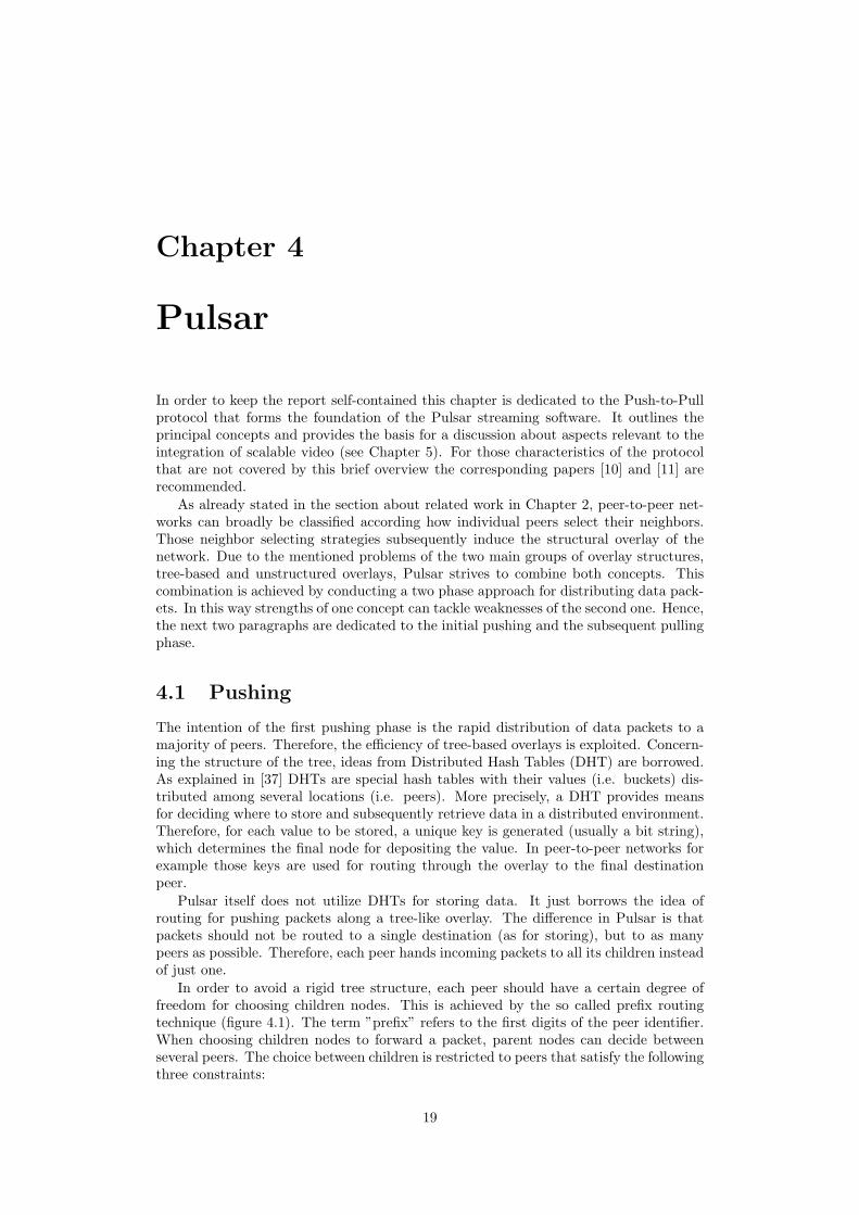
Chapter 1

Introduction

Networks with an underlying peer-to-peer structure (e.g. BitTorrent [1], Gnutella [2],eDonkey [3], Skype [4]) have evolved over the past few years to a point where theyform the basis for broadly used and established systems (e.g. Kazaa [5], LimeWire [6],Morpheus [7], eMule [8]). Thus, they are no longer solely of interest to the researchcommunity, but found their way to a wide range of mainstream applications. As peer-to-peer networks are gaining strength with a growing number of participants, theirpopularity will presumably not only sustain, but further rise.

The crucial feature of peer-to-peer networks that distinguishes them from conven-tional server-client architectures lies in their decentralized approach. Not a single serveris responsible for distributing the content, but every interconnected peer acts as clientand server at the same time. Therefore, a growing number of participants do not pro-duce a heavier burden on the network, as it is the case with central servers. The oppositeis true for peer-to-peer networks. Every new peer contributes more resources to the net-work, supporting the overall bandwidth and availability of content within the network.

The most widespread use of peer-to-peer networks can be found in the field of file-sharing systems ([5], [6], [7], [8]). They connect a vast amount of users for the purpose ofsharing (i.e. interchanging) files. While the idea of peer-to-peer enjoys great popularitywith file sharing systems the same cannot be confirmed when dealing with streamingcontent. Although the idea of peer-to-peer could equally well be expanded to streamingcontent, by now it is not yet a popular way of consuming audio or video sequencesdirectly (without downloading it first) over the Internet.

One of the main reasons behind this slower adaption of the peer-to-peer conceptin the field of streaming media lies in the inherent time-constrained nature of audioand video. In the case of only downloading a file, variations of bandwidth, only altersthe point in time when the file is completely available. Whereas the same fluctuationscan yield severe impacts on the perceptual quality of continuous audio or video streams.Thus, particular attention is required that the transfer of streaming content obeys certainrestrictions regarding a constant bit rate over time.

The peer-to-peer streaming software Pulsar [9] takes care of exactly those constraints.It connects the peers within the network through a special routing protocol ([10], [11])that strives to supply all members with a continuous stream of data. But managingand assuring a certain quality of service for all consumers within the network becomesa more challenging task as the requirements differ extensively between peers. They canvary among other points in regard to their local resources (e.g. computing power orscreen size) and in available network bandwidth (e.g. up or down link bit rate). Such avariety of needs can turn out a challenging task for a network protocol to serve.

This is where scalable video comes into play. One possible solution to the challengeof a diverse group of peers could be to provide several different versions of the samevideo stream, each tailored to specific end user capacities - so called simulcast. Besidesthe increasing complexity in managing all those versions, simulcast also causes the peer-

5

to-peer network to break apart. Since the various versions of the stream are conveyedcompletely independently from each other, peers requesting two different versions can nolonger support each other. Hence, the group breaks apart into several smaller groups -each for one version of the media stream in question. This fact makes switching betweendifferent bit rates of a video stream a complex task. It not only requires the refresh of allpacket buffers, it also induces the replacement of all neighbors. Therefore, adjusting thebit rate of a simulcasted video stream requires a complete reconstruction of the neighborstructure.

Scalable video strives to overcome this problem by avoiding the partition of peersaccording to their capabilities. With scalable video the different versions of a media file(in this case video) are consecutively build upon each other and therefore provide meansfor serving a variety of bit rates with a single stream. This increasing flexibility preventsthe network from breaking apart and therefore simplifies the adjustment to the right bitrate.

This master thesis studies the characteristics of scalable video and what advantagesit brings to applications in peer-to-peer environments. Furthermore a prototype imple-mentation of a scalable video decoder in connection with Pulsar and comparing resultsfrom various test runs are presented. In addition the necessary modifications to thepeer-to-peer protocol of Pulsar which enable the use of scalable video are discussed.

The remaining report is structured as follows: the following Chapter 2 provides anoverview of already published work on the topic of scalable video in relationship withpeer-to-peer networks. Chapter 3 introduces basic ideas of scalable video with specificfocus on the Scalable Video Coding (SVC) extention of the H.264/AVC standard. Inorder to provide the necessary basis for further discussions, Chapter 4 gives a briefoverview over the concepts behind the peer-to-peer streaming software Pulsar. Buildingon these explanations, Chapter 5 reviews those parts of Pulsar that were affected bythe integration of scalable video. Chapters 6 and 7 finish the report by, respectively,presenting results from evaluation test runs and by giving a conclusion on the conductedwork.

6

Chapter 2

Related Work

Papers related to the application of scalable video in peer-to-peer networks can broadlybe categorized into three groups. The first one is comprised by publications out of thescalable video domain. Whereas the second group concentrates on the topic of peer-to-peer networks. Bringing both fields together forms a third group, which covers thedeployment of scalable video standards in peer-to-peer networks.

2.1 Scalable Video

Probably the most important representative out of the first group would be the ScalableVideo Coding (SVC) standard from the Joint Video Team (JVT). It originated froma proposal ([12], [13]) of the Heinrich-Hertz-Institute, which is part of the FraunhoferInstitute in Berlin. In its latest version the SVC standard is integrated as an amendmentinto the H.264/AVC specification [14]. A brief overview of the standard is provided inthe subsequent paragraph of this report, while a more detailed outline is given by thepaper of H. Schwarz, D. Marpe and T.Wiegand from the Heinrich-Hertz-Institute [15].The reference software for the SVC standard (called Joint Scalable Video Model) canbe found on the Internet [16]. Several related papers with different focuses on SVC canbe found as well (Streaming: [17], Performance: [18], RTP: [19] and Mobile: [20]).

Another concept besides scalable video that is in some way related to it is MultiDescription Coding [21]. MDC has similar intensions like SVC - altering the bit rate ofa video - while using a completely different approach. The idea of MDC is to divide thecoded video into several sub streams (i.e. descriptions). Each description alone can bedecoded to a valid (but low quality) video stream. The final quality of the video improveswith the number of available descriptions, until all descriptions decoded together finallyform the original video stream.

The crucial difference of MDC to SVC lies in the prioritization of different parts ofthe video. While in SVC the layers bear a clear hierarchy (from the base layer to thelast enhancement layer) the opposite is true for different MDC descriptions. Therefore,all parts within a MDC coded bit stream are equally important and contribute thesame amount to the final quality. This property of MDC descriptions can be both: anadvantage or disadvantage. Beneficial is the fact that two distinct descriptions neverdepend on each other. That means no matter which descriptions are available; they canalways be assembled to form a valid video stream. The same is not possible with SVClayers, if one layer underneath is missing. On the other hand SVC utilized the fact thatnot all parts of a video are equally important to the final quality. Thus, it is possible toconvey the essential parts in the base layer with enhancement layers only adding detailsto the final video. Furthermore, data portioning of MDC demands a substantial amountof coding overhead and increases the complexity of the decoder. That is why MDC isnot yet considered by any of the traditional video coding standards.

7

2.2 Peer-to-Peer Networks

In the field of peer-to-peer networks the variety of scientific publications is even wider.Most peer-to-peer streaming networks of today use a neighbor selecting strategy thatcan be described as either tree-based or unstructured. Hence, first those two principalgroups of networks and their prominent representatives are introduced. Followed byprojects that - like Pulsar - apply Distributed Hash Tables (DHT) as a combination ofthose groups. Comprehensive overview papers discussing various types of peer-to-peerarchitectures are given by [22], [23] and [24].

Tree Based Overlays

Protocols based on a tree structure connect all peers via a rigid overlay. Each peer isobligated to forward incoming data packets to all of its children peers. Since the depthof such a tree stays rather small (logarithmic to the number of peers), information canbe transmitted rapidly to all members of the network. Generally, transmission of datapackets to other peers without having them explicitly requesting those packets is calleda push operation.

Two main disadvantages hinder the application of basic tree based protocols: onthe one hand maintenance overhead is large. Since the construction of a tree can be acomplex and time consuming task, they form rather static structures that react inflexibleif peers are constantly joining and leaving the network (called churn). The seconddrawback of trees is also related to their rigid nature: in their basic form each peer inthe tree is only connected to one single parent peer. This not only puts a heavy uploadburden on the parent node, it also makes the child node directly depended from theparent’s capacities. Hence, all peers following further down in the tree as well sufferfrom a weak predecessor peer. Besides, peers functioning as leafs of the tree have nochildren and can therefore receive packets without contributing to other peers.

Narada [25], Overcast [26], PeerCast [27] or FreeCast [28] can be considered typicalexamples of the first group, the tree based peer-to-peer streaming networks. To overcomethe problems imposed by a single tree structure, CoopNet [29] for example relies onmultiple trees. In addition CoopNet provides a certain degree of video scalability anderror resilience by coding the data in multiple descriptions (see section 2.3 on MultipleDescription Coding ). The same approach with MDC is also followed by the systemcalled Split Stream [30]. The overlay of CoolStreaming [31] does use a structured overlay,but it resembles more a mesh [32] than a conventional tree.

Unstructured Overlays

Due to the mentioned disadvantages of tree based peer-to-peer networks, some systemsavoid a rigid structure between the peers. Instead, each peer keeps just a list of its directneighbors while there exists no global overlay on top of all peers. As a result peers areonly aware of their direct neighbors. This leads to an improved flexibility in case ofchurn and avoids the time consuming task of setting up a tree structure. Moreover,peers joining or leave the network only cause very local modifications of the network.

Like tree-based overlays, also unstructured networks suffer from two downsides - bothrelated to a missing global structure for coordinating the distribution of data packets.First, in contrast to pushing, peers in an unstructured overlay must explicitly requestneeded packets (called pulling). Such notify-and-request communication between twopeers leads to an increased overhead and delays the delivery of packets. Second, due tothe lack of a global overlay special attention is needed that the network stays connectedas a whole. For example if peers strive to connect to neighbors that are physicallyclosely located, a worldwide network can very easily break apart into local sub-groups.Nevertheless, unstructured overlays are in most cases favored over tree based ones, dueto their better robustness against churn.

8

Two examples that follow the approach of an unstructured neighbor selection strat-egy are: Chainsaw [33] and GridMedia [34]. They differ primarily in the number ofneighbor nodes that each peer has to keep. Also file sharing protocols like BitTor-rent [1], Gnutella [2] and Napster [35] use similar concepts.

Distributed Hash Tables

Due to the mentioned disadvantages of tree-based and unstructured peer-to-peer net-works, Pulsar relies a combination of both concepts (see Section 4). The employedprefix routing algorithm is comprehensively explained in [11]. The idea of prefix rout-ing itself is based on the concept of Distributed Hash Tables (DHT). DHTs originatedfrom the routing algorithm of Plaxton [36], which was originally devised for managingof web queries. For an introduction to DHT or the latest developments in this field thereader is referred to [37] and [38] respectively. The first four systems that started to useDHT about the same time were: CAN [39], Chord [40], Pastry [41], and Tapestry [42].Especially the last two rely on routing algorithms simliar to the one used in Pulsar.

2.3 Scalable Video and Peer-to-Peer

Although both fields - scalable video as well as peer-to-peer networks - have attractedmuch attention from the research community, the amount of scientific papers focusingon their interaction is rather small. A very recent publication [43] employs SVC toguarantee smooth delivery of video content among the peers within the network. Theirperformance tests were carried out with a quality scalable video stream delivered over aGnutella like (i.e. unstructured) peer-to-peer network. The evaluation indeed shows animproved video throughput rate to the peers (measured in kBits/sec) and an enhancedquality of the received video (measured in Peak Signal To Noise Ratio - PSNR). Still,it should be pointed out, that like with Gnutella the topology among the peers is builtup arbitrarily (i.e. without a structured overlay).

The system described in [44] as well uses SVC in a peer-to-peer environment. Theirtheoretical analysis concentrates on quantifying the advantage of SVC with respect tosingle layer video coding. The quality gains are measured in PSNR and are calculateddepended on the bandwidth capacities of the peers. Especially in networks with aheterogeneous bandwidth distribution the strength of SVC becomes obvious. Theirpractical tests were conducted on the real time streaming protocol called Stanford Peer-to-Peer Multicast (SPPM) [45]. The results prove that especially in cases of a congestednetwork SVC outperforms single layer coding. That is due to fact that prioritizationof the layers allows to play at least the most important layers, even if the video is notcompletely received. Whereas, if bandwidth is not the bottle neck, single layer codingbenefits from its better coding efficiency.

Besides SVC, some interesting papers about MDC have been published in the contextof peer-to-peer. An older but still comprehensive overview of MDC video streaming inpeer-to-peer networks is given by [46]. The paper also compares MDC to the scalabilityfunctionality of MPEG-2 and MPEG-4 - the predecessor of the SVC standard today. Theapproach presented in [47] employs a method called flexible Multi Descriptions Coding(F-MDC) which is based on wavelet compression. F-MDC simplifies the partitioningof an encoded video stream into a specific number of descriptions. This video codec issubsequently deployed in a receiver centric (many to one) peer-to-peer network. A paperconcentrating more on the incentives aspect of MDC can be found in [48]. It is basedon the principal that peers contributing more to other peers also get a larger number ofdifferent descriptions and consequently enjoy a better video quality.

9

2.4 Commercial Peer-to-Peer Video Streaming

Currently many peer-to-peer clients are available on the web that offer free video stream-ing (but without the functionality for scalable video). Among the most prominent onesare systems like Zattoo [49], Tribler [50] or Joost [51]. All of them rely on similarconcepts: offering professional TV shows alongside private content and making moneythrough advertisement. The advantage for TV stations is that they can make theirprogram worldwide available, while shifting the costs for broadcasting to the individualusers. Also in Asia P2PTV applications like TVUPlayer [52], PPLive [53] or Cool-Streaming [31] are becoming more and more popular.

10

Chapter 3

Scalable Video

The term ”scalable” in the context of video stands for the general concept of coding animage sequence in a progressive (i.e. scalable) manner. Meaning, the internal structureof the coded video allows for a trade-off between bit rate and subjective quality. Theadditional flexibility is provided if parts of the video bit stream can be discarded withthe result still representing a valid video sequence. This requires a layered structurewithin the coded video that distinguishes basic information from parts that representonly details. In this way, a video can be adjusted in a fast and easy way to changingnetwork conditions or the specific capabilities of the end users. With this concept inmind, scalable video can also be compared to progressive JPEG [54] in the still imagedomain. Progressive JPEG offers the possibility to transmit the low frequency parts ofthe image first, giving a preliminary impression of what the final image would look like.All following higher frequency information builds upon the first version and accumulatesfiner details.

3.1 Benefits of Scalable Video

Previous to any further discussion about relevant aspects of encoding a video in a scalablemanner, the motivation behind this idea should be outlined. Broadly speaking, scalablein comparison to non-scalable videos provides the following advantages.

• In case of simulcasting, several different versions of the same video must be avail-able in order to serve diverse user requirements. Obviously those different versionsbear a high degree of redundancy. Although encoded for different bit rates, theyall represent the same content. Scalable video strives to reduce this redundancyand can therefore produce a video stream that requires significantly less storagespace than the sum over all versions of a simulcast video stream.

• In addition, scalable video streams can be encoded in a way to offer more than alimited number of different bit rate points (see Section 3.2.3 on Quality Scalability).With this fine graduation the choice among bit rates is expanded to a whole rangeof possible values.

• The management of different bit rate versions for the same video is avoided. Withscalable video just one bit stream can serve a diversity of client needs. As aconsequence the adjustment of the bit rate is simplified. It no longer involvesswitching between two separate bit streams, but can be carried out within thesame video stream. This convenience improves the flexibility of the video streamand increases the resilience against variations or failures of the transmission link.

• In representing the encoded video in a layered structure, scalable video assignsdifferent importance to each layer. The base layer of a scalable video stream

11

comprises information that is fundamental for the playback of the video. Thus,it represents the most important parts of the video stream. As the order of theenhancement layers on top increases their importance decreases.

The advantage of this layered structure is that specific parts of the encoded videostream can be prioritized. In a network environment with limited band widthcapacity this prioritization enables to prefer those data packets that are essentialfor the playback of the video. Hence, in cases were not enough band width isavailable to receive the whole video, scalable video offers at least a low qualityversion of that video.

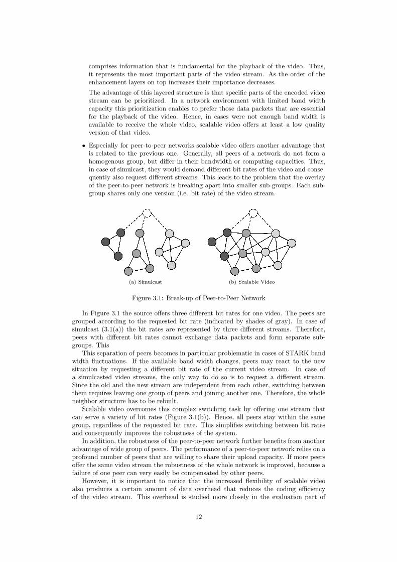
• Especially for peer-to-peer networks scalable video offers another advantage thatis related to the previous one. Generally, all peers of a network do not form ahomogenous group, but differ in their bandwidth or computing capacities. Thus,in case of simulcast, they would demand different bit rates of the video and conse-quently also request different streams. This leads to the problem that the overlayof the peer-to-peer network is breaking apart into smaller sub-groups. Each sub-group shares only one version (i.e. bit rate) of the video stream.

(a) Simulcast (b) Scalable Video

Figure 3.1: Break-up of Peer-to-Peer Network

In Figure 3.1 the source offers three different bit rates for one video. The peers aregrouped according to the requested bit rate (indicated by shades of gray). In case ofsimulcast (3.1(a)) the bit rates are represented by three different streams. Therefore,peers with different bit rates cannot exchange data packets and form separate sub-groups. This

This separation of peers becomes in particular problematic in cases of STARK bandwidth fluctuations. If the available band width changes, peers may react to the newsituation by requesting a different bit rate of the current video stream. In case ofa simulcasted video streams, the only way to do so is to request a different stream.Since the old and the new stream are independent from each other, switching betweenthem requires leaving one group of peers and joining another one. Therefore, the wholeneighbor structure has to be rebuilt.

Scalable video overcomes this complex switching task by offering one stream thatcan serve a variety of bit rates (Figure 3.1(b)). Hence, all peers stay within the samegroup, regardless of the requested bit rate. This simplifies switching between bit ratesand consequently improves the robustness of the system.

In addition, the robustness of the peer-to-peer network further benefits from anotheradvantage of wide group of peers. The performance of a peer-to-peer network relies on aprofound number of peers that are willing to share their upload capacity. If more peersoffer the same video stream the robustness of the whole network is improved, because afailure of one peer can very easily be compensated by other peers.

However, it is important to notice that the increased flexibility of scalable videoalso produces a certain amount of data overhead that reduces the coding efficiencyof the video stream. This overhead is studied more closely in the evaluation part of

12

Section 6.1.1. In addition, the complexity of scalable video encoders and decoders isconsiderable higher in comparison to their non-scalable counterparts.

After this brief analysis of the arguments for employing scalable video in peer-to-peernetworks, the remainder of this chapter concentrates on specific aspect of scalable video.

3.2 Scalable Video Coding Extension

Scalable video has been an active research area in the video coding community for morethan a decade (and still continues to do so). The latest standard out of this effortderives from the Joint Video Team (JVT) of the ITU-T Video Coding Group (VCEG)and the ISO/IEC Moving Picture Expert Group (MPEG). In 2007 they published thestandard called Scalable Video Coding (SVC)[14], which as an extension forms part ofthe H.264/AVC standard [55]. Since the SVC standard considers most of the aspects ofscalable video and furthermore plays an important role within the scalable video proto-type of Pulsar, the following paragraphs give a short overview over the basic conceptsfound in this standard.

As an extension SVC depends upon the main design decisions found in the regularH.264/AVC video coding standard. Therefore it reuses concepts like hybrid video cod-ing (i.e. inter-frame prediction in combination with intra-frame prediction), transformcoding or the underlying macro block structure. A detailed description of those princi-pals can be found in [55]. The core design concept of SVC which distinguishes it fromits parent standard is the layered structure of the coded video. Specific parts of thebit stream are grouped according to their importance on the final quality of the video.Within the SVC standard three different possibilities are described to divide the videointo several layers. In accordance with the SVC reference paper [15] this report uses theterm scalability dimensions for those three criteria. They are namely: Temporal Scala-bility, Spatial Scalability and Quality Scalability and will be described more closely inthe next few paragraphs.

3.2.1 Temporal Scalability

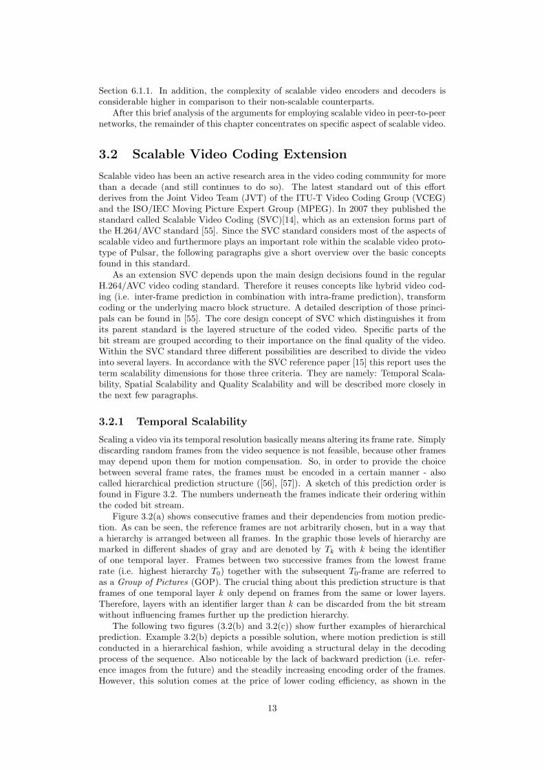
Scaling a video via its temporal resolution basically means altering its frame rate. Simplydiscarding random frames from the video sequence is not feasible, because other framesmay depend upon them for motion compensation. So, in order to provide the choicebetween several frame rates, the frames must be encoded in a certain manner - alsocalled hierarchical prediction structure ([56], [57]). A sketch of this prediction order isfound in Figure 3.2. The numbers underneath the frames indicate their ordering withinthe coded bit stream.

Figure 3.2(a) shows consecutive frames and their dependencies from motion predic-tion. As can be seen, the reference frames are not arbitrarily chosen, but in a way thata hierarchy is arranged between all frames. In the graphic those levels of hierarchy aremarked in different shades of gray and are denoted by Tk with k being the identifierof one temporal layer. Frames between two successive frames from the lowest framerate (i.e. highest hierarchy T0) together with the subsequent T0-frame are referred toas a Group of Pictures (GOP). The crucial thing about this prediction structure is thatframes of one temporal layer k only depend on frames from the same or lower layers.Therefore, layers with an identifier larger than k can be discarded from the bit streamwithout influencing frames further up the prediction hierarchy.

The following two figures (3.2(b) and 3.2(c)) show further examples of hierarchicalprediction. Example 3.2(b) depicts a possible solution, where motion prediction is stillconducted in a hierarchical fashion, while avoiding a structural delay in the decodingprocess of the sequence. Also noticeable by the lack of backward prediction (i.e. refer-ence images from the future) and the steadily increasing encoding order of the frames.However, this solution comes at the price of lower coding efficiency, as shown in the

13

evaluation part (Section 6) further down. In Figure 3.2(c) the frames are arranged in anon-dyadic way. Thus, the frame rate does not increase by a factor of 2 from one layerto the next.

Basically the concept of different temporal resolutions can just as well be achievedthrough pure H.264/AVC. The advanced flexibility of H.264/AVC for choosing and con-trolling reference frames [55] already enables the use of hierarchical motion prediction.SVC just adds methods of signaling and labeling the temporal layers in order to subse-quently extract them without difficulties.

(a) Four Temporal Layers

(b) Non-Delay Motion Predication

(c) Non-Dyadic Temporal Layers

Figure 3.2: Hierachical Motion Predication

3.2.2 Spatial Scalability

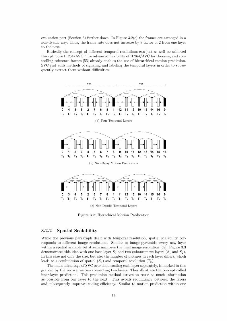
While the previous paragraph dealt with temporal resolution, spatial scalability cor-responds to different image resolutions. Similar to image pyramids, every new layerwithin a spatial scalable bit stream improves the final image resolution [58]. Figure 3.3demonstrates this idea with one base layer S0 and two enhancement layers (S1 and S2).In this case not only the size, but also the number of pictures in each layer differs, whichleads to a combination of spatial (Sk) and temporal resolution (Tk).

The main advantage of SVC over simulcasting each layer separately, is marked in thisgraphic by the vertical arrows connecting two layers. They illustrate the concept calledinter-layer prediction. This prediction method strives to reuse as much informationas possible from one layer to the next. This avoids redundancy between the layersand subsequently improves coding efficiency. Similar to motion prediction within one

14

layer, in the case of inter-layer prediction first the final image is predicted from thecorresponding picture in the reference layer and only the differences to the actual image(also called residuals) are finally encoded.

Figure 3.3: Three Spatial Layers

The most efficient way to perform inter-layer prediction would be to depend on thecompletely reconstructed or decoded picture from the layer underneath. This straightforward method, however, would significantly increase the complexity of the decoder, dueto the requirement of fully decoding all underlying layers. In order to keep the decodingprocess simple and avoid multiple decoding loops, the SVC standard provides inter-layer prediction methods that permit so called single-loop motion compensation. Withsingle-loop compensation, motion estimation at the encoder is conducted in all layers,while the expensive process of motion compensation at the decoder is only required inthe target layer. This is guaranteed if information from the lower layers can be usedin the target layer without decoding. Though single loop motion compensation slightlydecreases coding efficiency, it significantly simplifies the structure of the decoder [59],[60]. Hence, the following three inter-layer prediction techniques recycle informationfrom low level layers without entirely decoding them.

Inter-Layer Motion Prediction

When thinking of conventional motion prediction from H.264/AVC and similar stan-dards, there are two main components that are encoded for each B or P (i.e. motionpredicted) macro block: the motion vector and the corresponding residual information.In accordance with this, the first two inter-layer prediction methods concentrate on thosetwo parts. Since motion vectors are not likely to change too much from one layer tothe next (except for the scaling factor), they offer a good opportunity to reduce redun-dancy. Inter-layer motion prediction makes use of this fact by copying motion vectorsand additional information (macro block partition and reference picture indices) to lay-ers that are further up the hierarchy. After rescaling, the copied motion informationeither functions as prediction for the actual motion vectors or is directly used for motioncompensation.

Inter-Layer Residual Prediction

In addition to motion vectors SVC also provides means for reusing residual information.Therefore only the difference signal to the up scaled residual from the lower layer needsto be encoded. Although inter-layer motion and residual prediction together exploitmost of the information present in the lower layer, it is still not necessary to decode thereference layer. Hence, the concept of single loop motion compensation is still satisfied.

15

Inter-Layer Intra Prediction

This prediction technique goes one step further. Inter-layer intra prediction applies areconstructed version of the corresponding picture in the reference layer as prediction.This does require the decoding of the lower layer and is therefore only allowed for intrapredicted macro blocks. Those kinds of macro blocks are predicted without motionreferences to other frames, which guarantees that they can be decoded without runninga separate motion compensation loop.

3.2.3 Quality Scalability

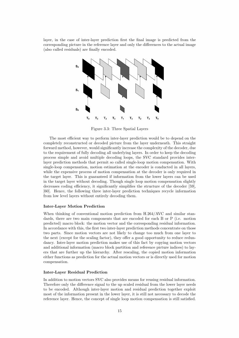
During encoding the textural information for each macro block is transformed to the fre-quency domain. For efficiency reasons those transform coefficients are quantized beforethey are finally encoded. In this way, the coefficients are mapped to a limited number ofquantization levels. What quality scalability (also called fidelity or signal-to-noise scal-ability) basically does is influencing the number of these quantization levels. Thereby,quality scalability achieves refinement in image quality through gradual downsizing ofthe quantization steps. Smaller quantization steps yield more quantization levels andconsequently a finer graduation of the transform coefficients (Figure 3.4). This leadsfinally to an improved image quality with a higher degree of details.

(a) Four Quantization Levels (b) Ten Quantization Levels

Figure 3.4: Quantization of Transform Coefficients

Looking more closely, this method can be considered a special case of spatial scalabil-ity. If the image resolution does not change from one spatial layer to the next, refinementis also solely achieved through smaller quantization steps. This approach of dividing thevideo into several quality layers is called Coarse Grain Scalability (CGS). Therefore,CGS layers can be considered special cases of spatial layers. One disadvantage of CGSis inherent to spatial scalable layers. Motion estimation is conducted in each spatiallayer separately (see Figure 3.5(a)), which makes switching between two spatial layersonly possible at well defined points within the video stream (i.e. at I-frames). Anotherdrawback of CGS is already revealed by its name: the choice among different bit ratesis limited to the number of CGS-layers. Fine graduation in between two CGS layers isnot possible.

Hence, the SVC draft also considers other means for quality scalability besides CGS.All those alternatives take place within one spatial layer and therefore all quality layersrely on the same motion compensation loop. In Figures 3.5(b), 3.5(c) and 3.5(d) thisfact is pointed out by the lack of gaps between the quality layers. Because all qualitylayers within the same spatial layer are based on the same motion prediction loop, thecrucial question then is, which quality level of the reference picture is used for motioncompensation?

16

(a) Coarse Grain Scalability (b) Fine Grain Scalability

(c) Drift (d) Medium Grain

Figure 3.5: Different Quality Scalability Methods

One possible solution called Fine Grain Scalability (FGS) is exemplified in Fig-ure 3.5(b). FGS always performs motion compensation on the lowest quality level of thereference picture. The advantage of FGS is that motion estimation at the encoder andmotion compensation at the decoder always use the same quality level of the referencepicture. This is guaranteed by the fact that at least the base layer is always available atthe receiver. If motion prediction is only conducted in the lowest fine grain quality layer,a loss of refinement packets (e.g. in the third frame of Figure 3.5(b)) does not influencethe motion compensation loop. This fact allows to scale the bit rate of a video streamon a packet based level, by simply discarding specific packets out of the enhancementlayer. Therefore, FGS ensures that the encoder and decoder are synchronized at alltimes. However, the cost of this solution arises in a reduced coding efficiency, becausethe more accurate information from the quality enhancement layers cannot be exploitedfor motion prediction.

The obvious way to reuse as much information from the reference picture as pos-sible would be to perform motion prediction in the highest of the quality layers. Thistechnique together with its major disadvantage can be seen in Figure 3.5(c). While thereference picture is used in a very efficient way, the video stream becomes susceptiblefor a phenomenon called drift. Drift describes a situation when the encoder and decodermotion predictions loops are no longer working on the same reference images (i.e. arerunning out of synch). If some packets of the enhancement layer have been discardedduring transmission, the decoder cannot detect this situation and applies a lower qualityreference picture for motion compensation as the encoder did. In Figure 3.5(c) motionestimation at the encoder is conducted in the enhancement layer, while for the thirdframe only the base layer arrives at the decoder. Hence, the reference picture of thefourth frame is incomplete, which can lead to visual artifacts in the decoded video se-quence. Furthermore, the effects due to drift accumulate over time, leading to a severeloss in video quality over time.

Therefore, SVC introduces a tradeoff between CGS and FGS, in order to fine tunethe video quality, while keeping the drift at an acceptable level. The idea of the so calledMedium Grain Scalability (MGS) concept is depicted in Figure 3.5(d). The improvementin respect to the already mentioned FGS lies in the flexibility to choose, which quality

17

layer is employed for motion prediction. In this way motion prediction can still beconducted in the enhancement layer, but with periodic updates in the base layer. Thoseperiodic updates happen at so called key pictures and synchronize the decoder motioncompensation loop with the one from the encoder. In Figure 3.5(d) at every fourthframe is a key picture where motion prediction is synchronised by updates in the baselayer. Thus, MGS guarantees that the effects of drift are not getting too acute.

3.2.4 Combination of the Scalability Dimensions

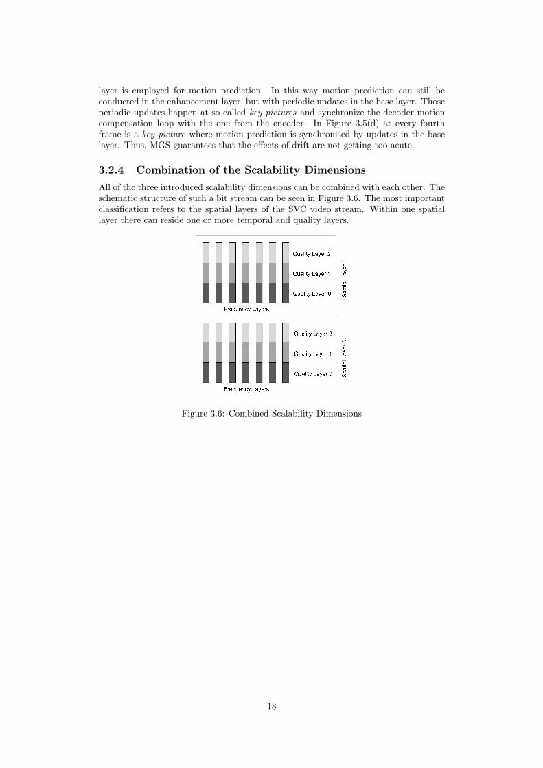
All of the three introduced scalability dimensions can be combined with each other. Theschematic structure of such a bit stream can be seen in Figure 3.6. The most importantclassification refers to the spatial layers of the SVC video stream. Within one spatiallayer there can reside one or more temporal and quality layers.

Figure 3.6: Combined Scalability Dimensions

18

Chapter 4

Pulsar

In order to keep the report self-contained this chapter is dedicated to the Push-to-Pullprotocol that forms the foundation of the Pulsar streaming software. It outlines theprincipal concepts and provides the basis for a discussion about aspects relevant to theintegration of scalable video (see Chapter 5). For those characteristics of the protocolthat are not covered by this brief overview the corresponding papers [10] and [11] arerecommended.

As already stated in the section about related work in Chapter 2, peer-to-peer net-works can broadly be classified according how individual peers select their neighbors.Those neighbor selecting strategies subsequently induce the structural overlay of thenetwork. Due to the mentioned problems of the two main groups of overlay structures,tree-based and unstructured overlays, Pulsar strives to combine both concepts. Thiscombination is achieved by conducting a two phase approach for distributing data pack-ets. In this way strengths of one concept can tackle weaknesses of the second one. Hence,the next two paragraphs are dedicated to the initial pushing and the subsequent pullingphase.

4.1 Pushing

The intention of the first pushing phase is the rapid distribution of data packets to amajority of peers. Therefore, the efficiency of tree-based overlays is exploited. Concern-ing the structure of the tree, ideas from Distributed Hash Tables (DHT) are borrowed.As explained in [37] DHTs are special hash tables with their values (i.e. buckets) dis-tributed among several locations (i.e. peers). More precisely, a DHT provides meansfor deciding where to store and subsequently retrieve data in a distributed environment.Therefore, for each value to be stored, a unique key is generated (usually a bit string),which determines the final node for depositing the value. In peer-to-peer networks forexample those keys are used for routing through the overlay to the final destinationpeer.

Pulsar itself does not utilize DHTs for storing data. It just borrows the idea ofrouting for pushing packets along a tree-like overlay. The difference in Pulsar is thatpackets should not be routed to a single destination (as for storing), but to as manypeers as possible. Therefore, each peer hands incoming packets to all its children insteadof just one.

In order to avoid a rigid tree structure, each peer should have a certain degree offreedom for choosing children nodes. This is achieved by the so called prefix routingtechnique (figure 4.1). The term ”prefix” refers to the first digits of the peer identifier.When choosing children nodes to forward a packet, parent nodes can decide betweenseveral peers. The choice between children is restricted to peers that satisfy the followingthree constraints:

19

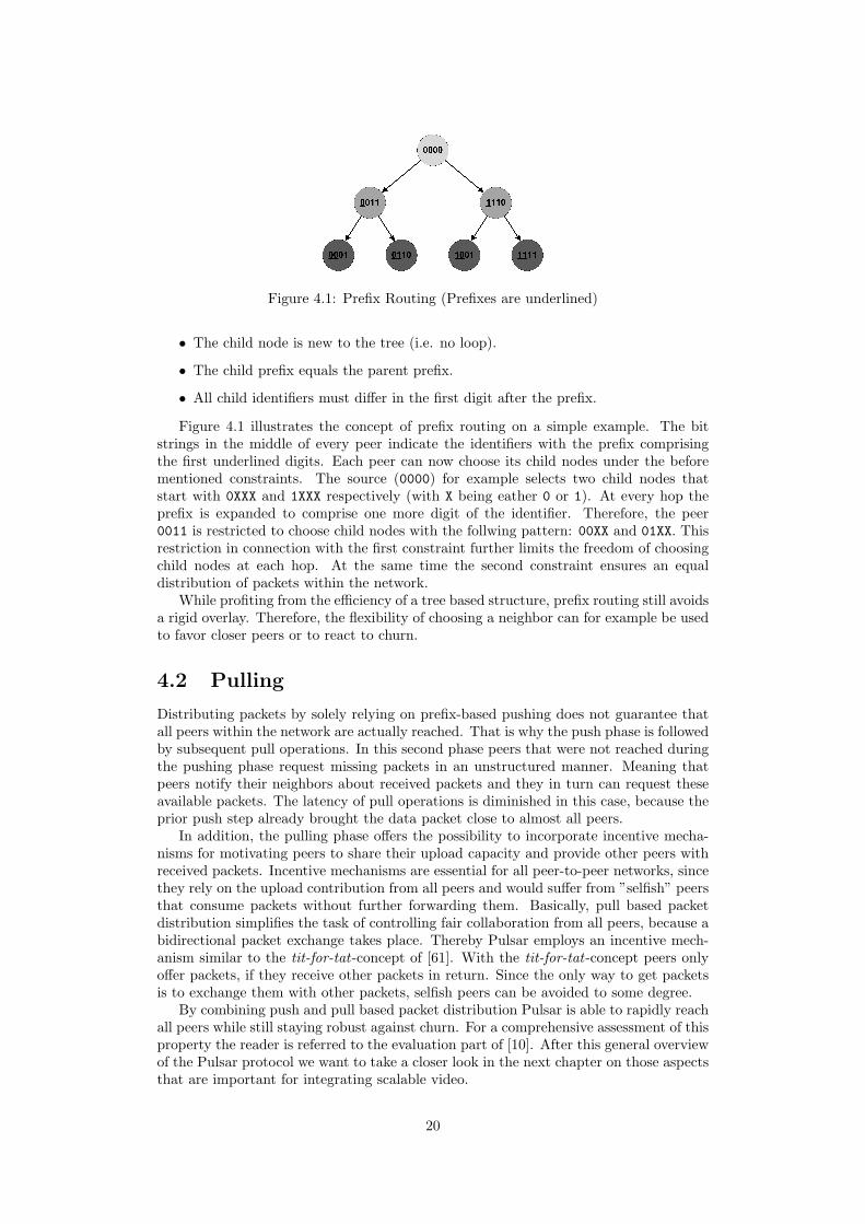
Figure 4.1: Prefix Routing (Prefixes are underlined)

• The child node is new to the tree (i.e. no loop).

• The child prefix equals the parent prefix.

• All child identifiers must differ in the first digit after the prefix.

Figure 4.1 illustrates the concept of prefix routing on a simple example. The bitstrings in the middle of every peer indicate the identifiers with the prefix comprisingthe first underlined digits. Each peer can now choose its child nodes under the beforementioned constraints. The source (0000) for example selects two child nodes thatstart with 0XXX and 1XXX respectively (with X being eather 0 or 1). At every hop theprefix is expanded to comprise one more digit of the identifier. Therefore, the peer0011 is restricted to choose child nodes with the follwing pattern: 00XX and 01XX. Thisrestriction in connection with the first constraint further limits the freedom of choosingchild nodes at each hop. At the same time the second constraint ensures an equaldistribution of packets within the network.

While profiting from the efficiency of a tree based structure, prefix routing still avoidsa rigid overlay. Therefore, the flexibility of choosing a neighbor can for example be usedto favor closer peers or to react to churn.

4.2 Pulling

Distributing packets by solely relying on prefix-based pushing does not guarantee thatall peers within the network are actually reached. That is why the push phase is followedby subsequent pull operations. In this second phase peers that were not reached duringthe pushing phase request missing packets in an unstructured manner. Meaning thatpeers notify their neighbors about received packets and they in turn can request theseavailable packets. The latency of pull operations is diminished in this case, because theprior push step already brought the data packet close to almost all peers.

In addition, the pulling phase offers the possibility to incorporate incentive mecha-nisms for motivating peers to share their upload capacity and provide other peers withreceived packets. Incentive mechanisms are essential for all peer-to-peer networks, sincethey rely on the upload contribution from all peers and would suffer from ”selfish” peersthat consume packets without further forwarding them. Basically, pull based packetdistribution simplifies the task of controlling fair collaboration from all peers, because abidirectional packet exchange takes place. Thereby Pulsar employs an incentive mech-anism similar to the tit-for-tat-concept of [61]. With the tit-for-tat-concept peers onlyoffer packets, if they receive other packets in return. Since the only way to get packetsis to exchange them with other packets, selfish peers can be avoided to some degree.

By combining push and pull based packet distribution Pulsar is able to rapidly reachall peers while still staying robust against churn. For a comprehensive assessment of thisproperty the reader is referred to the evaluation part of [10]. After this general overviewof the Pulsar protocol we want to take a closer look in the next chapter on those aspectsthat are important for integrating scalable video.

20

Chapter 5

SVC and Pulsar

The last two sections concentrated on scalable video and Pulsar separately. In thefollowing paragraphs both fields are brought together by discussing the actual modifi-cations that were necessary in order to integrate scalable video streams into Pulsar. Allnecessary modifications are dealing eather with Pulsar or the JSVM reference software.Thus, the follwing two paragraphs concentrate on those topics respectively.

Although this chapter almost exclusively talks about scalability in the field of video,all concepts were designed to be as generic as possible. This offers the possibility toexpand the idea of scalability to other media content types such as audio. Furthermore,a different scalable video format could be used as well. Only in places where SVC isexplicitly mentioned the discussion is restricted to the scalable video coding standard ofthe same name.

5.1 Modifications concerning Pulsar

The following modifications on the Pulsar protocol presented in Section 4 were necessaryin order to integrate scalable video streams. They can either be classified as concerningthe Push-to-Pull protocol or the layered structure of a video stream. Adaptations to theprotocol of Pulsar consider the modified communication between peers, when distribut-ing a scalable video stream. In addition, the internal layered structure of a scalablevideo stream demands further attention besides the protocol.

5.1.1 Protocol

Theoretically, a scalable video stream could be transmitted via the same overlay struc-ture, which is also used for non-scalable streams. But to fully benefit from the possibleadvantages of scalable video, the protocol has to consider the fact that peers might re-quest different layers of the same video stream. Thus, the following paragraphs describethose parts of the Pulsar protocol that need to be expanded in order to handle peersrequesting different layers.

Neighbor Selection

Each peer within the Pulsar network keeps its own list of neighboring peers (see Sec-tion 5.1.2). This group of peers is not only used to select children nodes for pushingpackets, but also for exchanging packets during the pull phase of packet distribution.Hence, the composition of this group strongly influences the distribution of packets inthe Pulsar network. In order to gradually improve the group of neighbors with respectto the available bandwidth and to adjust to variation within the group, Pulsar providesmeans for periodically updating the members of the group. Therefore, all neighbors are

21

ordered according to a specific criterion and those neighbors that appear at the end ofthe list are replaced by other peers.

Thus, the composition of neighbors is determined by two aspects: the strategy forscoring current neighbors and the strategy for scoring candidates for possible new neigh-bors. In Pulsar both scoring strategies can be implemented separately by the so calledNeighbor Scoring Strategy and the Candidates Scoring Strategy, respectively. Hence,neighbors with a low value according to the Neighbor Scoring Strategy are likely to bereplaced by peers that perform well with respect to the Candidates Scoring Strategy. Forscalable video streams it is important that both strategies also take the number of layersthat each neighbor offers into account. In order to fully benefit from the advantagesthat scalable video offers, two new strategies were devised: Scalable Neighbor ScoringStrategy and Scalable Candidates Scoring Strategy.

The Scalable Neighbor Scoring Strategy has to consider the fact that only neighborsfrom the same or higher layers can provide all packets needed to play a specific layer.Although for example neighbors from the base layer can assist in constructing the baselayer, their contribution is not sufficient to receive any enhancement layer. Since theScalable Neighbor Scoring Strategy determines which neighbors are replaced by newpeers, it is therefore important to ensure that at least one peer from the same or higherlayers remains in the group of neighbors.

In particular, the Scalable Neighbor Scoring Strategy of Pulsar implements this con-straint using a little trick. Usually all peers are scored according to their upload capacity.Only if one neighbor is the last one from the group of neighbors that offers the same ora higher layer, this peer obtains a virtual bandwidth boost. This boost guarantees thatthe Scalable Neighbor Scoring Strategy never chooses this neighbor for replacement.

Candidates Selection

The Candidates Scoring Strategy used by Pulsar for non-scalable video streams, relieson the computation of the packet Round Trip Time (RTT) to neighbor candidates.Thus, locality is taken into account in selection new neighbors by preferring peers witha shorter RTT. The reason behind using RTT is that information about the availablebandwidth is not known prior to any packet exchange over a longer period of time.

In case of the Scalable Candidates Scoring Strategy the number of layers plays aneven more important role. Generally all peers strive to connect to peers, who are in thesame or higher layers. Therefore, initially only peers from the same or higher layers areconsidered as neighbor candidates. Within one layer the candidates are scored accoringthe RTT similar to non-scalable streams. Only if no more peers from the same or higherlayers are available, peers from lower layers are chosen as new neighbors.

Since the source of a scalable video stream determines the maximum number oflayers, this Scalable Candidates Scoring Strategy aims at distributing packets first tothe higher layers and subsequently also supply lower layers. Figure 5.1 illustrates thisconcept on an example with three layers (the source is marked with a white point).

The idea behind this Candidates Scoring Strategy is two-folded.

• First, it can be assumed that peers in the highest layer have a high bandwidthat their disposal. Therefore, distribution among them can be conducted in a fastand efficient way. As soon as all peers in the higher layers are reached, they canfurther support colleagues from layers underneath. In this way the packets arerapidly distributed to as much peers as possible, which helps in reaching everypeer in a short period.

• Second, without a preference for peers in the same (or higher) layers, clustering ofpeers that only request the base layer becomes a threat. This happens due to thefact that only peers from higher layers can entirely serve peers from lower layersand not the other way around. Peers in the lowest layer only receive packets fromthe base layer of the video stream and therefore cannot support any requests for

22

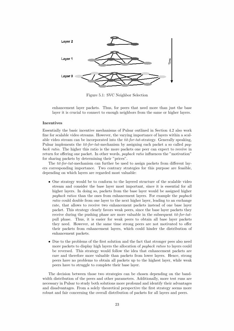
Figure 5.1: SVC Neighbor Selection

enhancement layer packets. Thus, for peers that need more than just the baselayer it is crucial to connect to enough neighbors from the same or higher layers.

Incentives

Essentially the basic incentive mechanisms of Pulsar outlined in Section 4.2 also workfine for scalable video streams. However, the varying importance of layers within a scal-able video stream can be incorporated into the tit-for-tat-strategy. Generally speaking,Pulsar implements the tit-for-tat-mechanism by assigning each packet a so called pay-back ratio. The higher this ratio is the more packets one peer can expect to receive inreturn for offering one packet. In other words, payback ratio influences the ”motivation”for sharing packets by determining their ”prices”.

The tit-for-tat-mechanism can further be used to assign packets from different lay-ers corresponding importance. Two contrary strategies for this purpose are feasible,depending on which layers are regarded most valuable:

• One strategy would be to conform to the layered structure of the scalable videostream and consider the base layer most important, since it is essential for allhigher layers. In doing so, packets from the base layer would be assigned higherpayback ratios than the ones from enhancement layers. For example the paybackratio could double from one layer to the next higher layer, leading to an exchangerate, that allows to receive two enhancement packets instead of one base layerpacket. This strategy clearly favors weak peers, since the base layer packets theyreceive during the pushing phase are more valuable in the subsequent tit-for-tat-pull phase. Thus, it is easier for weak peers to obtain all base layer packetsthey need. However, at the same time strong peers are not motivated to offertheir packets from enhancement layers, which could hinder the distribution ofenhancement packets.

• Due to the problems of the first solution and the fact that stronger pees also needmore packets to display high layers the allocation of payback ratios to layers couldbe reversed. This strategy would follow the idea that enhancement packets arerare and therefore more valuable than packets from lower layers. Hence, strongpeers have no problems to obtain all packets up to the highest layer, while weakpeers have to struggle to complete their base layer.

The decision between those two strategies can be chosen depending on the band-width distribution of the peers and other parameters. Additionally, more test runs arenecessary in Pulsar to study both solutions more profound and identify their advantagesand disadvantages. From a solely theoretical perspective the first strategy seems morerobust and fair concerning the overall distribution of packets for all layers and peers.

23

5.1.2 Layered Video Stream

In addition to the protocol aspcets the internal layered structure of a scalable videostream bears further challenges for Pulsar in comparison to single layer video streams(i.e. H.264/AVC). For the remaining of this report the term ”frame” refers to a set oflayers that together form a complete picture of the final video sequence.

Parts

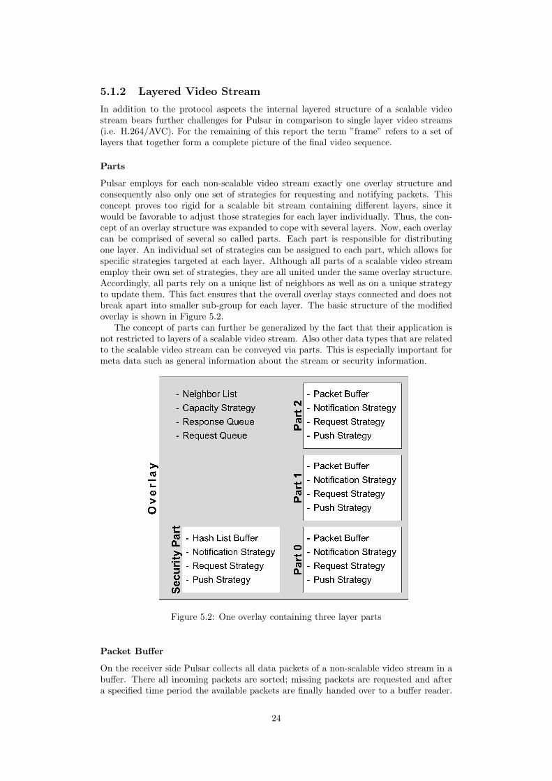
Pulsar employs for each non-scalable video stream exactly one overlay structure andconsequently also only one set of strategies for requesting and notifying packets. Thisconcept proves too rigid for a scalable bit stream containing different layers, since itwould be favorable to adjust those strategies for each layer individually. Thus, the con-cept of an overlay structure was expanded to cope with several layers. Now, each overlaycan be comprised of several so called parts. Each part is responsible for distributingone layer. An individual set of strategies can be assigned to each part, which allows forspecific strategies targeted at each layer. Although all parts of a scalable video streamemploy their own set of strategies, they are all united under the same overlay structure.Accordingly, all parts rely on a unique list of neighbors as well as on a unique strategyto update them. This fact ensures that the overall overlay stays connected and does notbreak apart into smaller sub-group for each layer. The basic structure of the modifiedoverlay is shown in Figure 5.2.

The concept of parts can further be generalized by the fact that their application isnot restricted to layers of a scalable video stream. Also other data types that are relatedto the scalable video stream can be conveyed via parts. This is especially important formeta data such as general information about the stream or security information.

Figure 5.2: One overlay containing three layer parts

Packet Buffer

On the receiver side Pulsar collects all data packets of a non-scalable video stream in abuffer. There all incoming packets are sorted; missing packets are requested and aftera specified time period the available packets are finally handed over to a buffer reader.

24

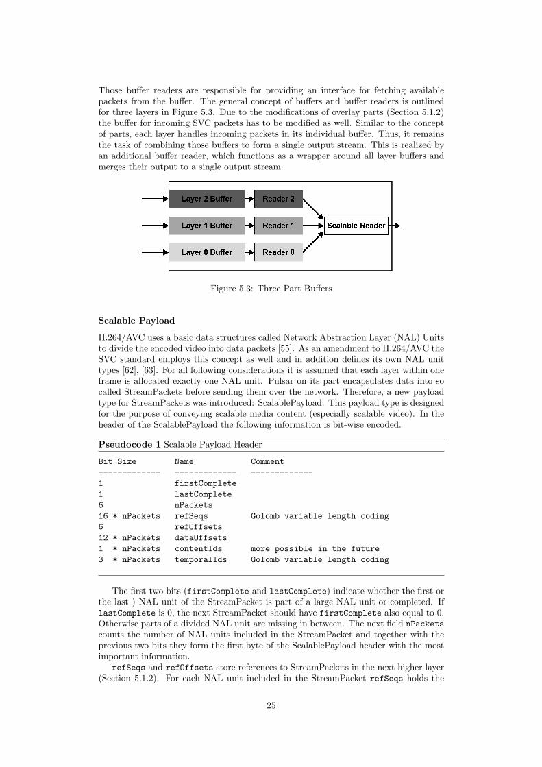
Those buffer readers are responsible for providing an interface for fetching availablepackets from the buffer. The general concept of buffers and buffer readers is outlinedfor three layers in Figure 5.3. Due to the modifications of overlay parts (Section 5.1.2)the buffer for incoming SVC packets has to be modified as well. Similar to the conceptof parts, each layer handles incoming packets in its individual buffer. Thus, it remainsthe task of combining those buffers to form a single output stream. This is realized byan additional buffer reader, which functions as a wrapper around all layer buffers andmerges their output to a single output stream.

Figure 5.3: Three Part Buffers

Scalable Payload

H.264/AVC uses a basic data structures called Network Abstraction Layer (NAL) Unitsto divide the encoded video into data packets [55]. As an amendment to H.264/AVC theSVC standard employs this concept as well and in addition defines its own NAL unittypes [62], [63]. For all following considerations it is assumed that each layer within oneframe is allocated exactly one NAL unit. Pulsar on its part encapsulates data into socalled StreamPackets before sending them over the network. Therefore, a new payloadtype for StreamPackets was introduced: ScalablePayload. This payload type is designedfor the purpose of conveying scalable media content (especially scalable video). In theheader of the ScalablePayload the following information is bit-wise encoded.

Pseudocode 1 Scalable Payload Header

Bit Size Name Comment------------- ------------- -------------1 firstComplete1 lastComplete6 nPackets16 * nPackets refSeqs Golomb variable length coding6 refOffsets12 * nPackets dataOffsets1 * nPackets contentIds more possible in the future3 * nPackets temporalIds Golomb variable length coding

The first two bits (firstComplete and lastComplete) indicate whether the first orthe last ) NAL unit of the StreamPacket is part of a large NAL unit or completed. IflastComplete is 0, the next StreamPacket should have firstComplete also equal to 0.Otherwise parts of a divided NAL unit are missing in between. The next field nPacketscounts the number of NAL units included in the StreamPacket and together with theprevious two bits they form the first byte of the ScalablePayload header with the mostimportant information.

refSeqs and refOffsets store references to StreamPackets in the next higher layer(Section 5.1.2). For each NAL unit included in the StreamPacket refSeqs holds the

25

sequence number of the StreamPacket that contains the next higher NAL unit. Thisinformation is important for the scalable reader (Section 5.1.2) to reconstructe all layersfrom the base up to the last enhancement layer. The references are likely to increaseonly by one or at most a few steps from one NAL unit to the next. That is why onlythe first value is directly encoded and for all subsequent references only the difference tothe prior value is conveyed. Furthermore, Golomb variable length entropy coding [64]is employed to further reduce the necessary bits. In addition to the sequence numberreferences, refOffsets points to the first NAL unit in the next higher StreamPacketthat depends on the current StreamPacket. This information is necessary for recoveryafter packet losses (see next next Section 5.1.2).

In order to safe further bytes ScalablePayload does not separate NAL units using theusual H.264/AVC three bytes delimiter 001. Instead dataOffsets indicates the limitsbetween several NAL units. The following bit contentIds is yet always equal to 0, butin the future it is intended to distinguish between audio and video data. In additioncontentId could be expanded to comprise more than one bit in order to support othercontent types as well (e.g. speech, meta information or subtitles). At the end of theheader, the fields temporalIds signal to which temporal layer each of the followingNAL units belong. This information enables the extraction of a specific temporal layerwithout the need for parsing any of the NAL units. The difference between the valuesfor temporalIds are also likely to differ only by one. Therefore, the same variable lengthcoding schema as for refSeqs is adopted.

Packeting of Scalable Payload

Besides the payload a new method for packing SVC NAL units into StreamPacketshad to be devised. For this propose different techniques tailored to specific needs weredeveloped. In all cases the maximum size of a StreamPacket is assumed to be 1350bytes.

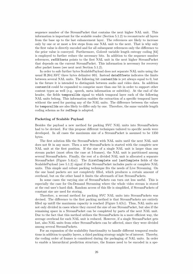
The first solution fills the StreamPackets with NAL units until the next NAL unitdoes not fit in any more. Then a new StreamPackets is started with the complete newNAL unit at the first position. If the size of a single NAL unit is larger than onestream packet (most often the case at I-frames), the NAL unit is partitioned amongseveral StreamPackets. Finally, the rest of a divided NAL unit is allocated a separateStreamPacket (Figure 5.4(a)). The firstComplete and lastComplete fields of theScalablePayload (see 5.1.2) signal if the StreamPacket includes parts or complete NALunits. This simple and robust packing technique fits the needs of Live Streaming. Onthe one hand packets are not completely filled, which produces a certain amount ofoverhead, but on the other hand it limits the aftermath of lost StreamPackets.

In some cases the varying size of StreamPackets can turn out less useful. This isespecially the case for On-Demand Streaming where the whole video stream is storedat the end user’s hard disk. Random access of this file is simplified, if StreamPackets ofconstant size are used for storing.

Therefore, a second method for packing SVC NAL units into StreamPackets wasdevised. The difference to the first packing method is that StreamPackets are entirelyfilled up untill the maximum capacity is reached (Figure 5.4(b)). Thus, NAL units arenot only divided in cases where they exceed the size of one StreamPacket, but also if theremaining space in a StreamPacket can be completed by parts of the next NAL unit.Due to the fact that this method utilizes the StreamPackets in a more efficient way, theaverage overhead for each NAL unit is reduced. However, if a single StreamPacket getslost, also NAL units from other StreamPackets can be affected, since they were dividedamong several StreamPackets.

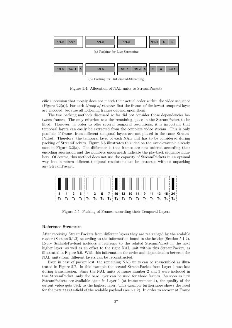
For an expansion of the scalability functionality to handle different temporal resolu-tions in addition to quality layers, a third packing strategy might be of interest. Thereby,the coding order of frames is considered during the packaging of NAL units. In orderto enable a hierarchical prediction structure, the frames need to be encoded in a spe-

26

(a) Packing for Live-Streaming

(b) Packing for OnDemand-Streaming

Figure 5.4: Allocation of NAL units to StreamPackets

cific succession that mostly does not match their actual order within the video sequence(Figure 3.2(a)). For each Group of Pictures first the frames of the lowest temporal layerare encoded, because all following frames depend upon them.

The two packing methods discussed so far did not consider those dependencies be-tween frames. The only criterion was the remaining space in the StreamPacket to befilled. However, in order to offer several temporal resolutions, it is important thattemporal layers can easily be extracted from the complete video stream. This is onlypossible, if frames from different temporal layers are not placed in the same Stream-Packet. Therefore, the temporal layer of each NAL unit has to be considered duringpacking of StreamPackets. Figure 5.5 illustrates this idea on the same example alreadyused in Figure 3.2(a). The difference is that frames are now ordered according theirencoding succession and the numbers underneath indicate the playback sequence num-bers. Of course, this method does not use the capacity of StreamPackets in an optimalway, but in return different temporal resolutions can be extracted without unpackingany StreamPacket.

Figure 5.5: Packing of Frames according their Temporal Layers

Reference Structure

After receiving StreamPackets from different layers they are rearranged by the scalablereader (Section 5.1.2) according to the information found in the header (Section 5.1.2).Every ScalablePayload includes a reference to the related StreamPacket in the nexthigher layer, as well as an offset to the right NAL unit within this StreamPacket, asillustrated in Figure 5.6. With this information the order and dependencies between theNAL units from different layers can be reconstructed.

Even in case of packet lost, the remaining NAL units can be reassembled as illus-trated in Figure 5.7. In this example the second StreamPacket from Layer 1 was lostduring transmission. Since the NAL units of frame number 2 and 3 were included inthis StreamPacket, only the base layer can be used for those frames. As soon as newStreamPackets are available again in Layer 1 (at frame number 4), the quality of theoutput video gets back to the highest layer. This example furthermore shows the needfor the refOffsets-field of the scalable payload (see 5.1.2). In order to recover at Frame

27

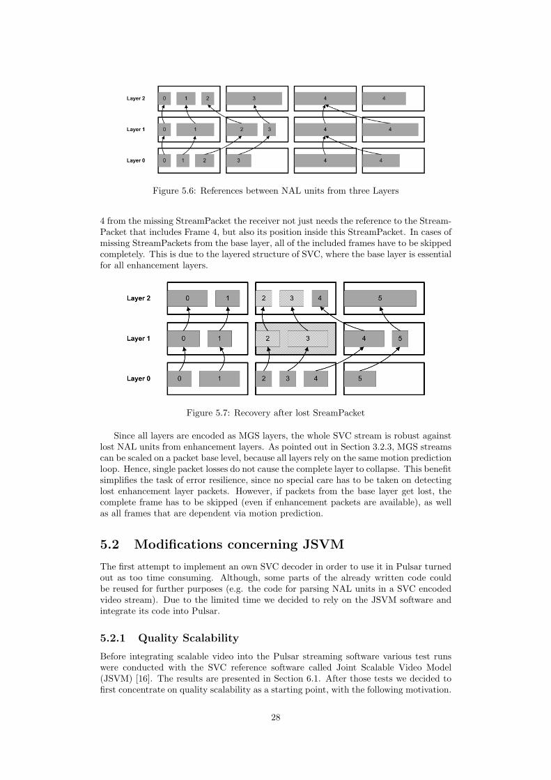
Figure 5.6: References between NAL units from three Layers

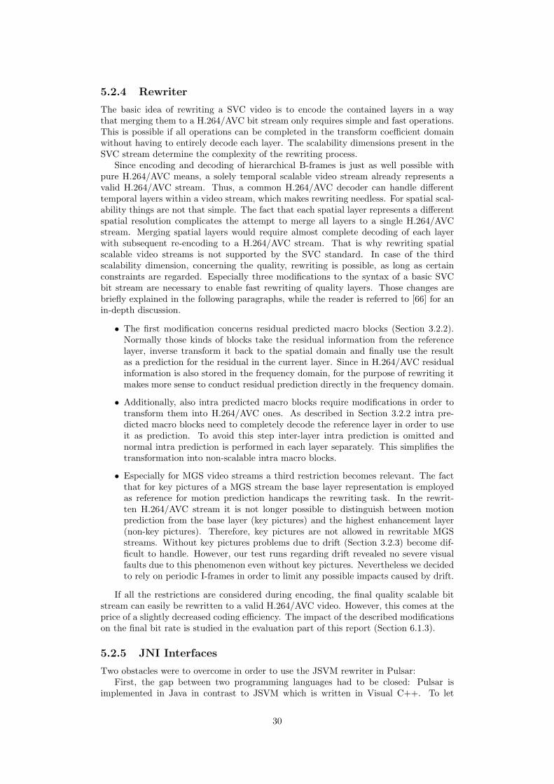
4 from the missing StreamPacket the receiver not just needs the reference to the Stream-Packet that includes Frame 4, but also its position inside this StreamPacket. In cases ofmissing StreamPackets from the base layer, all of the included frames have to be skippedcompletely. This is due to the layered structure of SVC, where the base layer is essentialfor all enhancement layers.

Figure 5.7: Recovery after lost SreamPacket

Since all layers are encoded as MGS layers, the whole SVC stream is robust againstlost NAL units from enhancement layers. As pointed out in Section 3.2.3, MGS streamscan be scaled on a packet base level, because all layers rely on the same motion predictionloop. Hence, single packet losses do not cause the complete layer to collapse. This benefitsimplifies the task of error resilience, since no special care has to be taken on detectinglost enhancement layer packets. However, if packets from the base layer get lost, thecomplete frame has to be skipped (even if enhancement packets are available), as wellas all frames that are dependent via motion prediction.

5.2 Modifications concerning JSVM

The first attempt to implement an own SVC decoder in order to use it in Pulsar turnedout as too time consuming. Although, some parts of the already written code couldbe reused for further purposes (e.g. the code for parsing NAL units in a SVC encodedvideo stream). Due to the limited time we decided to rely on the JSVM software andintegrate its code into Pulsar.

5.2.1 Quality Scalability

Before integrating scalable video into the Pulsar streaming software various test runswere conducted with the SVC reference software called Joint Scalable Video Model(JSVM) [16]. The results are presented in Section 6.1. After those tests we decided tofirst concentrate on quality scalability as a starting point, with the following motivation.

28

When scaling a video on the basis of its quality, the consumer may notice the lower bitrate by block patterns or other visual artifacts. However, the spatial and temporalresolution of the video sequence is kept intact, which guarantees a smooth playback.Furthermore, with medium grain scalability (MGS) the choices of different bit rates is notrestricted to the number of layers and the bit rate can be scaled on a packet based level.This feature essentially improves the flexibility of the scalable video stream and at thesame time makes it to some extent robust against lost packets. Although other scalabilityoptions (namely spatial and temporal scalability) as well offer interesting possibilities,quality scalability seems to best fit the requirements of a peer-to-peer environment.

5.2.2 Temporal Scalability

In contrast to Spatial and Quality Scalability, a standard H.264/AVC video streamcan already include different frame rates. Since hierarchical B-frames (Figure 3.2) canbe encoded by the sole use of H.264/AVC concepts, regular non-scalable decoders arealso capable of handling temporal scalable video streams. Especially for MGS streamstemporal scalability forms an integral part of the primarily quality scalable video stream.This is due to the fact that all frames from the lowest temporal layer are encoded askey frames (see Section 3.2.3). Motion prediction for key pictures is conducted in thebase quality layer in contrast to all other frames, where the highest quality is used forthis purpose. Therefore, every MGS stream offers quality and temporal scalability atthe same time. In order to make use of the temporal layers special methods for packingand signaling those layers are needed.

5.2.3 Decoding or Rewriting

Another interesting question that came up during testing the JSVM software was therelation of SVC and basic H.264/AVC. Since Pulsar is already working with the commonH.264/AVC decoder of FFmpeg [65], it would be nice to expand its functionality to alsocope with scalable video. In this way the redundancy of two parallel decoders - one forsingle layer H.264/AVC and one for SVC - could be avoided. One way to achieve thisgoal would be to directly integrate scalable video functionality into the existing code ofFFmpeg. Our efforts in this direction are still not finished yet, but under continuousprogress.

This report however concentrates on a second solution. Thereby a scalable bit streamis first transformed to a regular H.264/AVC stream and subsequently handed over tothe FFmpeg-decoder of Pulsar (see Figure 5.8). The specification of SVC considers suchrewriting concepts [66], which will be outlined in the following paragraph.

Figure 5.8: SVC-to-H.264 Rewriter

29

5.2.4 Rewriter

The basic idea of rewriting a SVC video is to encode the contained layers in a waythat merging them to a H.264/AVC bit stream only requires simple and fast operations.This is possible if all operations can be completed in the transform coefficient domainwithout having to entirely decode each layer. The scalability dimensions present in theSVC stream determine the complexity of the rewriting process.

Since encoding and decoding of hierarchical B-frames is just as well possible withpure H.264/AVC means, a solely temporal scalable video stream already represents avalid H.264/AVC stream. Thus, a common H.264/AVC decoder can handle differenttemporal layers within a video stream, which makes rewriting needless. For spatial scal-ability things are not that simple. The fact that each spatial layer represents a differentspatial resolution complicates the attempt to merge all layers to a single H.264/AVCstream. Merging spatial layers would require almost complete decoding of each layerwith subsequent re-encoding to a H.264/AVC stream. That is why rewriting spatialscalable video streams is not supported by the SVC standard. In case of the thirdscalability dimension, concerning the quality, rewriting is possible, as long as certainconstraints are regarded. Especially three modifications to the syntax of a basic SVCbit stream are necessary to enable fast rewriting of quality layers. Those changes arebriefly explained in the following paragraphs, while the reader is referred to [66] for anin-depth discussion.

• The first modification concerns residual predicted macro blocks (Section 3.2.2).Normally those kinds of blocks take the residual information from the referencelayer, inverse transform it back to the spatial domain and finally use the resultas a prediction for the residual in the current layer. Since in H.264/AVC residualinformation is also stored in the frequency domain, for the purpose of rewriting itmakes more sense to conduct residual prediction directly in the frequency domain.

• Additionally, also intra predicted macro blocks require modifications in order totransform them into H.264/AVC ones. As described in Section 3.2.2 intra pre-dicted macro blocks need to completely decode the reference layer in order to useit as prediction. To avoid this step inter-layer intra prediction is omitted andnormal intra prediction is performed in each layer separately. This simplifies thetransformation into non-scalable intra macro blocks.

• Especially for MGS video streams a third restriction becomes relevant. The factthat for key pictures of a MGS stream the base layer representation is employedas reference for motion prediction handicaps the rewriting task. In the rewrit-ten H.264/AVC stream it is not longer possible to distinguish between motionprediction from the base layer (key pictures) and the highest enhancement layer(non-key pictures). Therefore, key pictures are not allowed in rewritable MGSstreams. Without key pictures problems due to drift (Section 3.2.3) become dif-ficult to handle. However, our test runs regarding drift revealed no severe visualfaults due to this phenomenon even without key pictures. Nevertheless we decidedto rely on periodic I-frames in order to limit any possible impacts caused by drift.

If all the restrictions are considered during encoding, the final quality scalable bitstream can easily be rewritten to a valid H.264/AVC video. However, this comes at theprice of a slightly decreased coding efficiency. The impact of the described modificationson the final bit rate is studied in the evaluation part of this report (Section 6.1.3).

5.2.5 JNI Interfaces

Two obstacles were to overcome in order to use the JSVM rewriter in Pulsar:First, the gap between two programming languages had to be closed: Pulsar is

implemented in Java in contrast to JSVM which is written in Visual C++. To let

30

both applications collaborate with each other, we made use of the so called Java NativeInterface (JNI) [67]. This library provides interfaces that allow Java code running in thevirtual machine (JVM) to call functions written in a different programming language(i.e. native code like C++, C or other implementations). Also the opposite direction, anative program calling Java code, is possible through the JNI.

As far as it concerns the integration of the JSVM rewriter into Pulsar, we employedboth the writing and reading functionality of the JNI. The first one for sending packetsreceived by a Pulsar peer to the rewriter and the second one for subsequently collect-ing the rewritten H.264/AVC frame. The basic concept is seen in Figure 5.8. DirectByte Buffers are used as data structures for actually exchanging bytes between bothapplications (see Pseudocode 2).

Pseudocode 2 Rewriter Interface for waiting on available NAL units (C++)

// finding method for fetching next packet from PulsarfetchPacketMethod* = GetMethodID("fetchNextNALunit");

// actually waiting till next NAL unit is availablejavaObject* nalUnitByteBuffer = CallMethod(fetchPacketMethod);

// get address of new NAL unitunsigned char* nalUnitAddress = GetByteBufferAddress(nalUnitByteBuffer);

Second, the code of the JSVM rewriter had to be modified in order to work witha consecutive stream of video data. Before, the software assumed that a complete andfinished video file is available. In our solution the rewriter is now running parallel toPulsar waiting to rewrite one frame as soon as it is received. Code snippets for thisfunction are listed below (see Pseudocode 3).

Pseudocode 3 Pulsar Interface for sending available NAL units to Rewriter (Java)

public ByteBuffer fetchNextNALunit(){

ArrayList<ByteBuffer> availableNalUnits;

while(true){if(availableNalUnits.size > 0){availableNalUnits.returnFirstInLine();availableNalUnits.removeFirstInLine();

}}

}

For the actual integration into Pulsar a new FFmpeg-codec was generated, which usesthe rewriter to transform SVC NAL units into H.264/AVC ones. Therefore, FFmpeg canhandle SVC streams by simply utilizing the new rewriter-codec in connection with theregular H.264/AVC decoder. Furthermore, the interface outlined above is not restrictedto the JSVM rewriter. It could equally be expanded for encoding or completely decoding(not just rewrite) SVC bit streams. Nevertheless, the performance issues of the JSVMimplementation outlined in Section 7.1 should be pointed out as well.

31

32

Chapter 6

Evaluation

6.1 SVC Evaluation

All of the following test runs were conducted with the Joint Scalable Video Model(JSVM) - Version 9.12.2 - which serves as the reference software behind the SVC stan-dard. It is maintained by the Joint Video Team (JVT) and freely available over theInternet [16].

After conducting a few test runs with JSVM we recognized that the provided testsequences [68] are not representative enough for our purpose. In some test cases theirshort length of only a few seconds was not sufficient to produce stable results. Therefore,we created our own test sequence on the basis of the open source movie ElephantsDream [69] and the Trailor for the movie Michael Clayton.

Pseudocode 4 Main Configuration File for three MGS Layers

# JSVM Main Configuration File

OutputFile ed/ed_400x224.svc # Bitstream fileFrameRate 25.0 # Frame rateFramesToBeEncoded 1749 # Number of framesGOPSize 16 # GOP SizeIntraPeriod 32 # Intra Period

BaseLayerMode 1 # Base layer modeSearchMode 4 # Search modeSearchRange 32 # Search range

CgsSnrRefinement 1 # 1: MGS; 0: CGSEncodeKeyPictures 1 # 0:none, 1:MGS, 2:allMGSControl 2 # ME/MC for non-key pics

NumLayers 3 # Number of layersLayerCfg layer0.cfg # Layer 0 config fileLayerCfg layer1.cfg # Layer 1 config fileLayerCfg layer2.cfg # Layer 2 config file

33

6.1.1 Single Layer vs. Multiple Layers

The first question studied during the evaluation was concerning the overhead of scal-able video in comparison to non-scalable video streams. Therefore, several SVC testsequences with different numbers of quality layers (MGS) were compared to single layerH.264/AVC. In all test cases a resolution of 400 x 224 pixel was used with similarparameters to the ones presented in Pseudocode 4. All layers were encoded at a con-stant frame rate of 25 frames/sec. Furthermore, SVC-to-H.264/AVC rewriting abilitywas disabled (AvcRewriteFlag 0) and inter-layer prediction was set on to adaptive(InterLayerPred 2).

The most important parameter during encoding a quality scalable bit stream repre-sents the quantization parameter (called QP). This parameter influences the quantiza-tion of transform coefficients by specifying the quantization step size. Thus, a smallerQP value increases the number of quantization levels and consequently sustains moredetails of the original video in the encoded version. In particular, an increment of QPby 1 corresponds to a larger quantization step size of approximately 12% [70] and acorresponding decrease in bit rate of about the same percentage. Hence, a difference of6 QPs should lead to circa a doubling of bit rate (1.126 = 1.97).

Figure 6.1 illustrates the overhead induced by SVC, by comparing different QP valueswith their corresponding bit rates. For both test sequences (Elephants Dream and Lost)the bit rates of the non-scalable bit streams are illustrated as single points. In contrastto SVC streams, they are not connected via a curve in order to clarify that they representseparate streams. Each of these H.264/AVC streams was encoded with a different QPranging from 38 to 26. Thus, for H.264/AVC streams the lowest bit rate (128 kBits/sec)forms roughly 1/4 of the highest one (512 kBits/sec).

(a) Elephants Dream Test Sequence (b) Lost Test Sequence

Figure 6.1: SVC overhead in comparison to H.264/AVC

Taking a look at the SVC video streams (illustrated as solid curves in Figure 6.1),it can be seen, that in all cases the lowest layer (i.e. the base layer) comprises the samebit rate as the base H.264/AVC version does. This is not surprising since the base layerof a SVC video always represents a valid H.264/AVC stream. However, when addingmore layers to the SVC stream, a certain amount of overhead compared to H.264/AVCbecomes apparent.

The most important characteristic of the three SVC streams illustrated in additionto the H.264/AVC stream is their number of MGS layers. The more different bit ratesa SVC stream offers, the higher is its overhead in comparison to the correspondingH.264/AVC version. When concentrating on the highest bit rate (i.e. QP of 26) the fol-lowing overhead (as percentage) can be measured for the Elephants Dream test sequence:

34

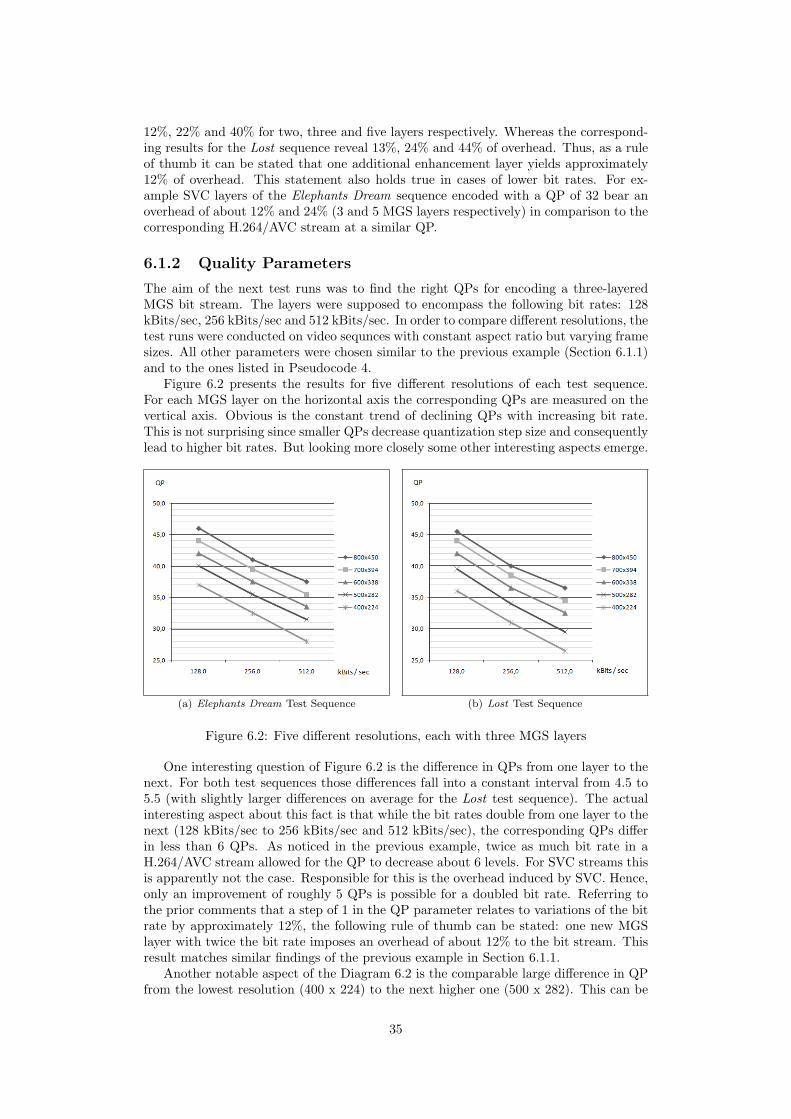
12%, 22% and 40% for two, three and five layers respectively. Whereas the correspond-ing results for the Lost sequence reveal 13%, 24% and 44% of overhead. Thus, as a ruleof thumb it can be stated that one additional enhancement layer yields approximately12% of overhead. This statement also holds true in cases of lower bit rates. For ex-ample SVC layers of the Elephants Dream sequence encoded with a QP of 32 bear anoverhead of about 12% and 24% (3 and 5 MGS layers respectively) in comparison to thecorresponding H.264/AVC stream at a similar QP.

6.1.2 Quality Parameters

The aim of the next test runs was to find the right QPs for encoding a three-layeredMGS bit stream. The layers were supposed to encompass the following bit rates: 128kBits/sec, 256 kBits/sec and 512 kBits/sec. In order to compare different resolutions, thetest runs were conducted on video sequnces with constant aspect ratio but varying framesizes. All other parameters were chosen similar to the previous example (Section 6.1.1)and to the ones listed in Pseudocode 4.

Figure 6.2 presents the results for five different resolutions of each test sequence.For each MGS layer on the horizontal axis the corresponding QPs are measured on thevertical axis. Obvious is the constant trend of declining QPs with increasing bit rate.This is not surprising since smaller QPs decrease quantization step size and consequentlylead to higher bit rates. But looking more closely some other interesting aspects emerge.

(a) Elephants Dream Test Sequence (b) Lost Test Sequence

Figure 6.2: Five different resolutions, each with three MGS layers

One interesting question of Figure 6.2 is the difference in QPs from one layer to thenext. For both test sequences those differences fall into a constant interval from 4.5 to5.5 (with slightly larger differences on average for the Lost test sequence). The actualinteresting aspect about this fact is that while the bit rates double from one layer to thenext (128 kBits/sec to 256 kBits/sec and 512 kBits/sec), the corresponding QPs differin less than 6 QPs. As noticed in the previous example, twice as much bit rate in aH.264/AVC stream allowed for the QP to decrease about 6 levels. For SVC streams thisis apparently not the case. Responsible for this is the overhead induced by SVC. Hence,only an improvement of roughly 5 QPs is possible for a doubled bit rate. Referring tothe prior comments that a step of 1 in the QP parameter relates to variations of the bitrate by approximately 12%, the following rule of thumb can be stated: one new MGSlayer with twice the bit rate imposes an overhead of about 12% to the bit stream. Thisresult matches similar findings of the previous example in Section 6.1.1.

Another notable aspect of the Diagram 6.2 is the comparable large difference in QPfrom the lowest resolution (400 x 224) to the next higher one (500 x 282). This can be

35

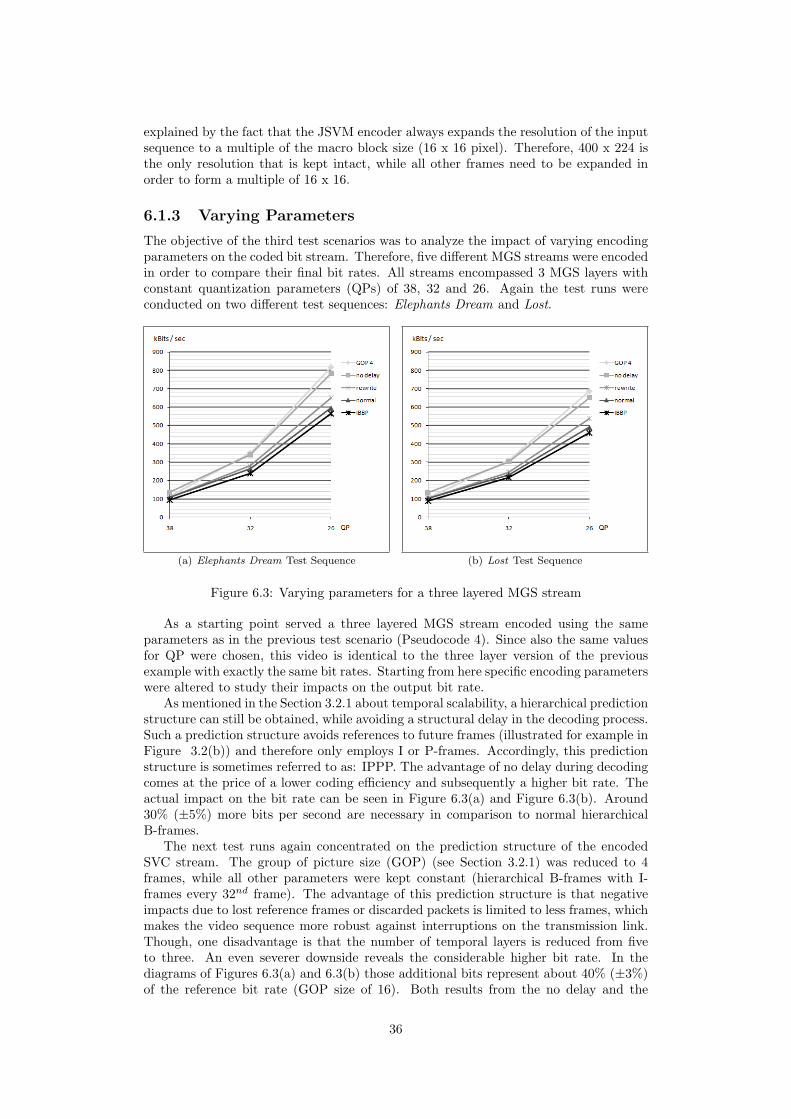
explained by the fact that the JSVM encoder always expands the resolution of the inputsequence to a multiple of the macro block size (16 x 16 pixel). Therefore, 400 x 224 isthe only resolution that is kept intact, while all other frames need to be expanded inorder to form a multiple of 16 x 16.

6.1.3 Varying Parameters

The objective of the third test scenarios was to analyze the impact of varying encodingparameters on the coded bit stream. Therefore, five different MGS streams were encodedin order to compare their final bit rates. All streams encompassed 3 MGS layers withconstant quantization parameters (QPs) of 38, 32 and 26. Again the test runs wereconducted on two different test sequences: Elephants Dream and Lost.

(a) Elephants Dream Test Sequence (b) Lost Test Sequence

Figure 6.3: Varying parameters for a three layered MGS stream

As a starting point served a three layered MGS stream encoded using the sameparameters as in the previous test scenario (Pseudocode 4). Since also the same valuesfor QP were chosen, this video is identical to the three layer version of the previousexample with exactly the same bit rates. Starting from here specific encoding parameterswere altered to study their impacts on the output bit rate.

As mentioned in the Section 3.2.1 about temporal scalability, a hierarchical predictionstructure can still be obtained, while avoiding a structural delay in the decoding process.Such a prediction structure avoids references to future frames (illustrated for example inFigure 3.2(b)) and therefore only employs I or P-frames. Accordingly, this predictionstructure is sometimes referred to as: IPPP. The advantage of no delay during decodingcomes at the price of a lower coding efficiency and subsequently a higher bit rate. Theactual impact on the bit rate can be seen in Figure 6.3(a) and Figure 6.3(b). Around30% (±5%) more bits per second are necessary in comparison to normal hierarchicalB-frames.

The next test runs again concentrated on the prediction structure of the encodedSVC stream. The group of picture size (GOP) (see Section 3.2.1) was reduced to 4frames, while all other parameters were kept constant (hierarchical B-frames with I-frames every 32nd frame). The advantage of this prediction structure is that negativeimpacts due to lost reference frames or discarded packets is limited to less frames, whichmakes the video sequence more robust against interruptions on the transmission link.Though, one disadvantage is that the number of temporal layers is reduced from fiveto three. An even severer downside reveals the considerable higher bit rate. In thediagrams of Figures 6.3(a) and 6.3(b) those additional bits represent about 40% (±3%)of the reference bit rate (GOP size of 16). Both results from the no delay and the

36

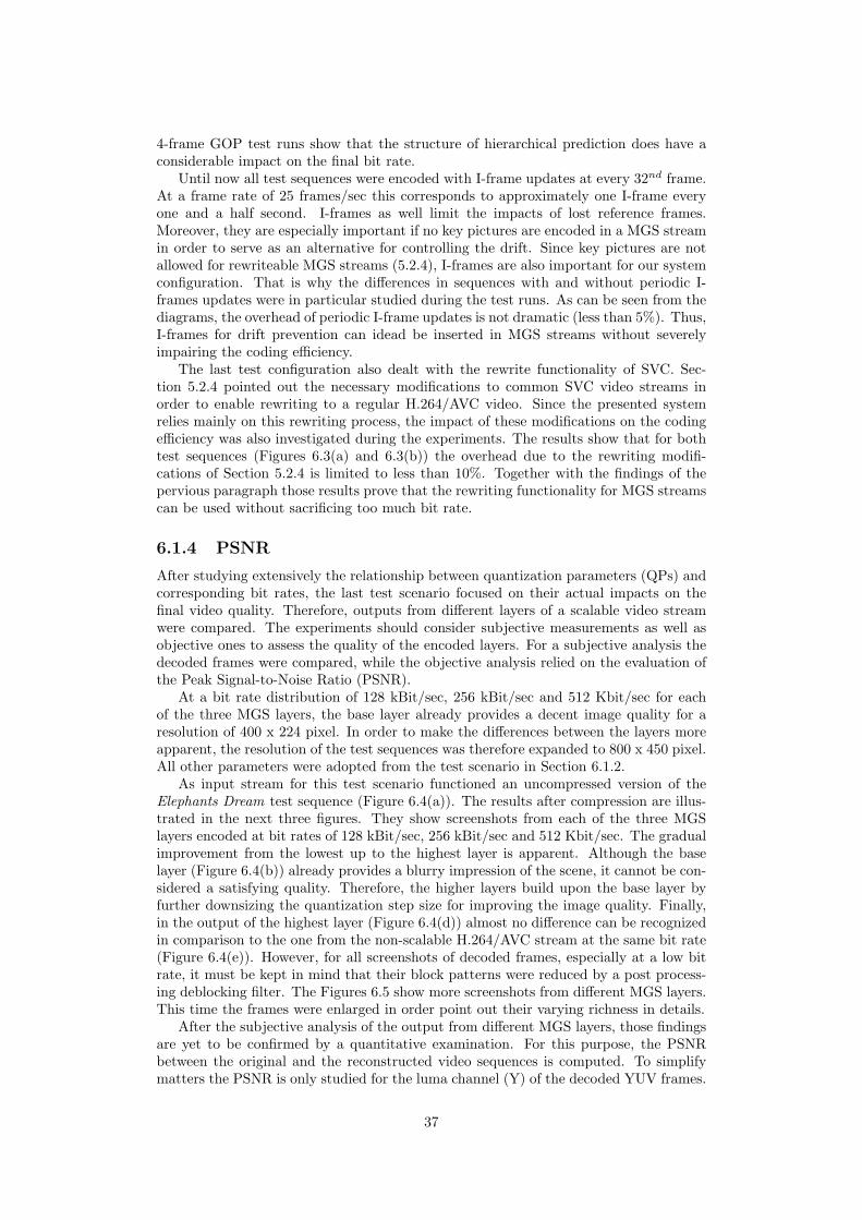
4-frame GOP test runs show that the structure of hierarchical prediction does have aconsiderable impact on the final bit rate.

Until now all test sequences were encoded with I-frame updates at every 32nd frame.At a frame rate of 25 frames/sec this corresponds to approximately one I-frame everyone and a half second. I-frames as well limit the impacts of lost reference frames.Moreover, they are especially important if no key pictures are encoded in a MGS streamin order to serve as an alternative for controlling the drift. Since key pictures are notallowed for rewriteable MGS streams (5.2.4), I-frames are also important for our systemconfiguration. That is why the differences in sequences with and without periodic I-frames updates were in particular studied during the test runs. As can be seen from thediagrams, the overhead of periodic I-frame updates is not dramatic (less than 5%). Thus,I-frames for drift prevention can idead be inserted in MGS streams without severelyimpairing the coding efficiency.

The last test configuration also dealt with the rewrite functionality of SVC. Sec-tion 5.2.4 pointed out the necessary modifications to common SVC video streams inorder to enable rewriting to a regular H.264/AVC video. Since the presented systemrelies mainly on this rewriting process, the impact of these modifications on the codingefficiency was also investigated during the experiments. The results show that for bothtest sequences (Figures 6.3(a) and 6.3(b)) the overhead due to the rewriting modifi-cations of Section 5.2.4 is limited to less than 10%. Together with the findings of thepervious paragraph those results prove that the rewriting functionality for MGS streamscan be used without sacrificing too much bit rate.

6.1.4 PSNR

After studying extensively the relationship between quantization parameters (QPs) andcorresponding bit rates, the last test scenario focused on their actual impacts on thefinal video quality. Therefore, outputs from different layers of a scalable video streamwere compared. The experiments should consider subjective measurements as well asobjective ones to assess the quality of the encoded layers. For a subjective analysis thedecoded frames were compared, while the objective analysis relied on the evaluation ofthe Peak Signal-to-Noise Ratio (PSNR).

At a bit rate distribution of 128 kBit/sec, 256 kBit/sec and 512 Kbit/sec for eachof the three MGS layers, the base layer already provides a decent image quality for aresolution of 400 x 224 pixel. In order to make the differences between the layers moreapparent, the resolution of the test sequences was therefore expanded to 800 x 450 pixel.All other parameters were adopted from the test scenario in Section 6.1.2.

As input stream for this test scenario functioned an uncompressed version of theElephants Dream test sequence (Figure 6.4(a)). The results after compression are illus-trated in the next three figures. They show screenshots from each of the three MGSlayers encoded at bit rates of 128 kBit/sec, 256 kBit/sec and 512 Kbit/sec. The gradualimprovement from the lowest up to the highest layer is apparent. Although the baselayer (Figure 6.4(b)) already provides a blurry impression of the scene, it cannot be con-sidered a satisfying quality. Therefore, the higher layers build upon the base layer byfurther downsizing the quantization step size for improving the image quality. Finally,in the output of the highest layer (Figure 6.4(d)) almost no difference can be recognizedin comparison to the one from the non-scalable H.264/AVC stream at the same bit rate(Figure 6.4(e)). However, for all screenshots of decoded frames, especially at a low bitrate, it must be kept in mind that their block patterns were reduced by a post process-ing deblocking filter. The Figures 6.5 show more screenshots from different MGS layers.This time the frames were enlarged in order point out their varying richness in details.

After the subjective analysis of the output from different MGS layers, those findingsare yet to be confirmed by a quantitative examination. For this purpose, the PSNRbetween the original and the reconstructed video sequences is computed. To simplifymatters the PSNR is only studied for the luma channel (Y) of the decoded YUV frames.

37

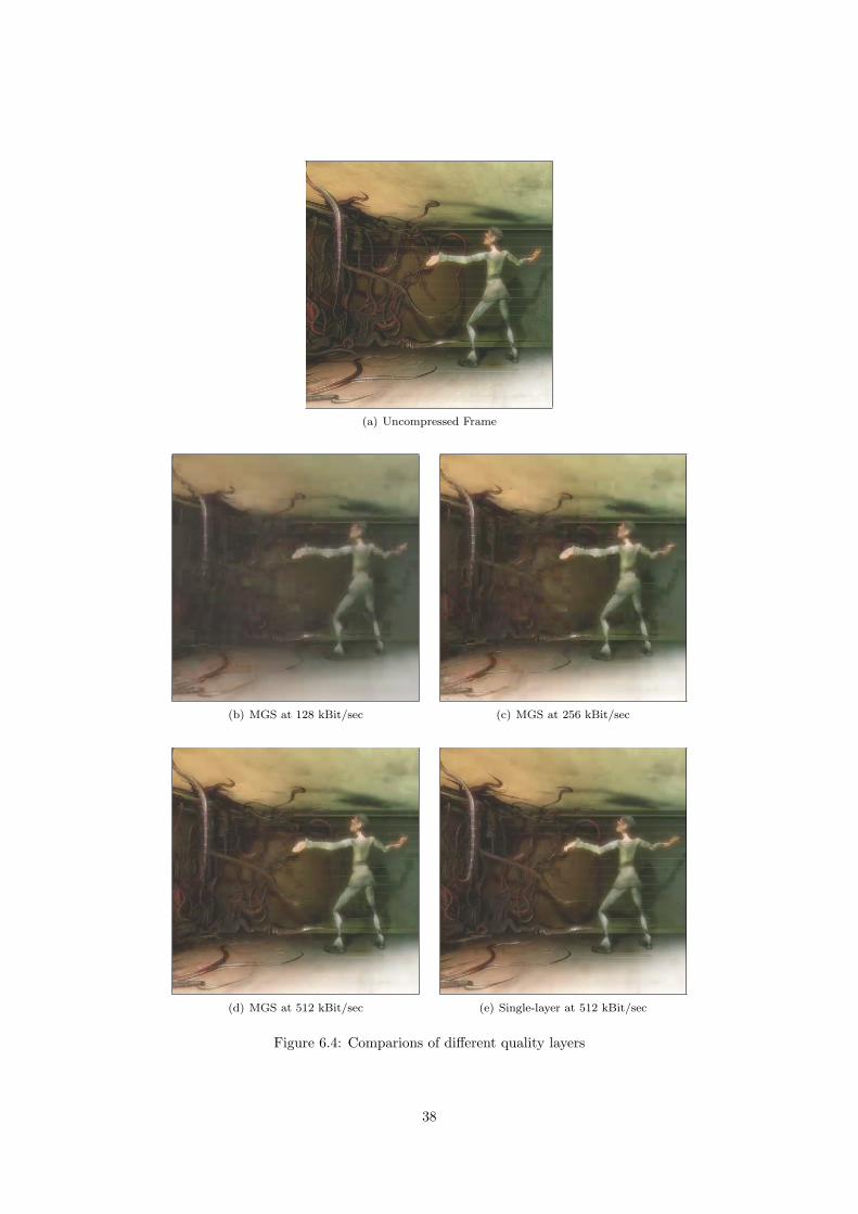
(a) Uncompressed Frame

(b) MGS at 128 kBit/sec (c) MGS at 256 kBit/sec

(d) MGS at 512 kBit/sec (e) Single-layer at 512 kBit/sec

Figure 6.4: Comparions of different quality layers

38

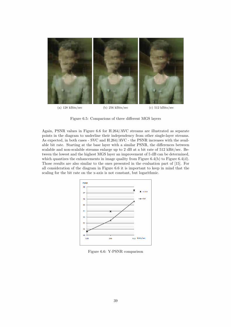
(a) 128 kBits/sec (b) 256 kBits/sec (c) 512 kBits/sec

Figure 6.5: Comparions of three different MGS layers

Again, PSNR values in Figure 6.6 for H.264/AVC streams are illustrated as separatepoints in the diagram to underline their independency from other single-layer streams.As expected, in both cases - SVC and H.264/AVC - the PSNR increases with the avail-able bit rate. Starting at the base layer with a similar PSNR, the differences betweenscalable and non-scalable streams enlarge up to 2 dB at a bit rate of 512 kBit/sec. Be-tween the lowest and the highest MGS layer an improvement of 5 dB can be determined,which quantizes the enhancements in image quality from Figure 6.4(b) to Figure 6.4(d).Those results are also similar to the ones presented in the evaluation part of [15]. Forall consideration of the diagram in Figure 6.6 it is important to keep in mind that thescaling for the bit rate on the x-axis is not constant, but logarithmic.

Figure 6.6: Y-PSNR comparison

39

6.2 Pulsar Evaluation

The foregoing set of test scenarios concentrated on SVC alone and on the impact thatcertain input parameters play on the scalable video stream. For a better understandingof the advantages that SVC brings to peer-to-peer networks and Pulsar in particular,further test runs were conducted. This second set of test scenarios focused on scalablevideo data sent over the Pulsar network. Therefore, test cases for assessing the impactof scalable video as a new feature were devised and verified in the Pulsar test bed. Fora better control of the data sent over the network, simulated data packets were usedinstead of actual video data. In doing so, it is possible to test different distributions ofdata packets to video layers.

6.2.1 Number of decoded bytes

Besides the increase flexibility of scalable video, Section 3.1 also mentioned anotheradvantage of scalable video: prioritization. In representing the encoded video in alayered structure, scalable video offers the possibility to play the video stream at leastat a low quality, if the complete video stream is not available.

In order to assess this benefit the same simulated video stream was distributedtwo times over the same network: the first time as a non-scalable H.264/AVC streamand the second time encoded as a three layered SVC stream. For the H.264/AVCstream a bit rate of 512 kBits/sec (64 kBytes/sec) was assumed, which corresponds toabout 600 kBits/sec (75 kBytes/sec) for the SVC stream due to the overhead. Thesimulated H.264/AVC stream was generated by packets with a constant size of 2560bytes. Whereas, for the SVC stream varying packet sizes were assumed that relate topackets of a regular SVC stream (i.e. larger packets at low temporal layers due to I andP-frames). In both cases the packet sizes sum up to 64 kBytes/sec and 75 kBytes/secrespectively at a frame rate of 25 frames/sec.

Figure 6.7: Numner of downloaded and decoded bytes

The decisive factor of the results presented in Figure 6.7 is the upload capacity of thepeers. This upload speed (measured in kBytes/sec) was assumed to be constant overall of the 50 peers simulated in this experiment. In the diagram the increasing uploadcapacity is compared with two values: the number of downloaded and the number ofdecoded bytes. Both values represent the average over all peers. For the H.264/AVCstream a frame was only considered decodable, if all proceeding frames up to the nextI-frame could be decoded as well. This prediction structure corresponds to a IPPPsuccession of frames. Whereas the underlying prediction structure for the SVC stream

40

were hierarchical B-frames (Section 3.2.1). Therefore, at least the base layer of all framesfrom lower temporal layers had to be available to consider a SVC frame decodable.

Up to the maximum bit rate of the H.264/AVC stream in both cases the same amountof bytes can be downloaded. This value is only restricted by the upload capacity for allpeers. The additional bytes beyond 64 kBytes/sec in case of the SVC stream representthe overhead for the scalable information.

When taking a look at the number of decoded bytes a significant difference betweenthe H.264/AVC and the SVC stream becomes apparent. Especially if the upload speedof the peers is strongly restricted, Figure 6.7 reveals that far more data of the SVCstream can be decoded for playback as it is the case with H.264/AVC. This is due to thefact that with scalable video the restricted bandwidth can be used in a more efficientway. While in a non-scalable video stream all bytes have the same prioritization, SVCcan concentrate the limited amount of bandwidth to those parts of the video that arenecessary to play at least a poor quality or a low frame rate. This is achieved if thelow layers (in respect of quality or temporal resolution) of the scalable video stream aredownloaded first, before any of the enhancement layers is requested.

Figure 6.8 illustrates the percentage of decodable data in respect to the overallamount of data arriving at the peers. In this case the more efficient use of down-loaded bytes is even more apparent. Starting at the lowest upload capacity always morethan half of the downloaded scalable video data can subsequently be decoded. For theH.264/AVC stream those values cannot be achieved until upload capacity of the peersreaches about 60 kBytes/sec.

Figure 6.8: Percentage of decoded data (downloaded data = 100%)

However, as the upload capacity further rises, the differences between the H.264/AVCand the SVC stream diminish. The reason behind this development has two aspects .First, with a growing bandwidth the prioritization of video data within the SVC streambecomes less important. Concentrating on the basic parts of a video stream is mainlybeneficial if only a small portion of the overall data is available. Second, if bandwidthbecomes less of a problem, the overhead of SVC is getting a more important issue. Atthe highest upload capacities more bytes have to be downloaded for a SVC stream inorder to achieve the best quality. This fact can also be seen in Figure 6.7 by the divergingdownload rates at an upload capacity of 70 kBytes/sec.

41

42

Chapter 7

Conclusion

This report discussed the up and downsides of Scalable Video Coding with particularattention to its application in peer-to-peer networks. In addition, the actual integra-tion of scalable video into an existing peer-to-peer streaming software, namely Pulsar,was presented. As a conclusion it can be stated that on the one hand scalable videoindeed has the potential to enhance the video streaming functionality of peer-to-peernetworks. In particular flexibility in bit rate and error resilience can benefit from such asystem. However, on the other hand increased coding complexity and considerable bitrate overhead have to be taken into account as well. Furthermore, due to its very recentapproval the SVC standard has not yet found its way to broad application in publiclyavailable systems. It remains to be seen if SVC can gain the same acceptance in videoapplications as its parent standard H.264/AVC is already enjoying.

7.1 Discussion

Though Pulsar is now able to handle scalable video streams, there is still room forfurther improvement. The most serious weak point of the system presented in theforegoing chapters, is clearly the dependency on the JSVM software. Especially threeissues can be stated that have to be solved before Pulsar can offer scalable video on abroad scale.

First, JSVM is intended as reference software. Hence, its main focus lies on clearlyrepresenting the SVC standard rather than on performance issues. This fact challengedour demand to run the rewriter in real time. We managed to rewrite video sequenceswith a resolution of 400 x 224 in real time. Clearly there should be a high potentialfor significant performance improvements, given that the rewriting process itself is nota complex one.

Second, for the test runs so far a SVC bit stream was assumed to be given. Nev-ertheless, for actual application of SVC in Pulsar this issues needs to be reconsidered.One possible solution would be to keep the encoder out of Pulsar and further rely onexternal encoders like the one from JSVM. Due to the mentioned performance issuesof JSVM this way is unlikely to provide a completely satisfying solution. Furthermore,the user interface of the JSVM encoder turns out to be too complicated for ”main-stream” application. More promising but also obliged with a higher effort would be analternative tailored specifically to Pulsar. As discussed in [71], a similar solution to therewriter could be possible at the encoder side as well. This would include a rewritingprocess from H.264/AVC to SVC. Although special considerations concerning drift haveto be regarded, rewriting to SVC is probably faster than completely encoding from anuncompressed video stream. Furthermore, this solution could be combined with alreadyexisting and established H.264/AVC encoders.

When further pursuing the idea of H.264/AVC to SVC rewriting, the system could

43

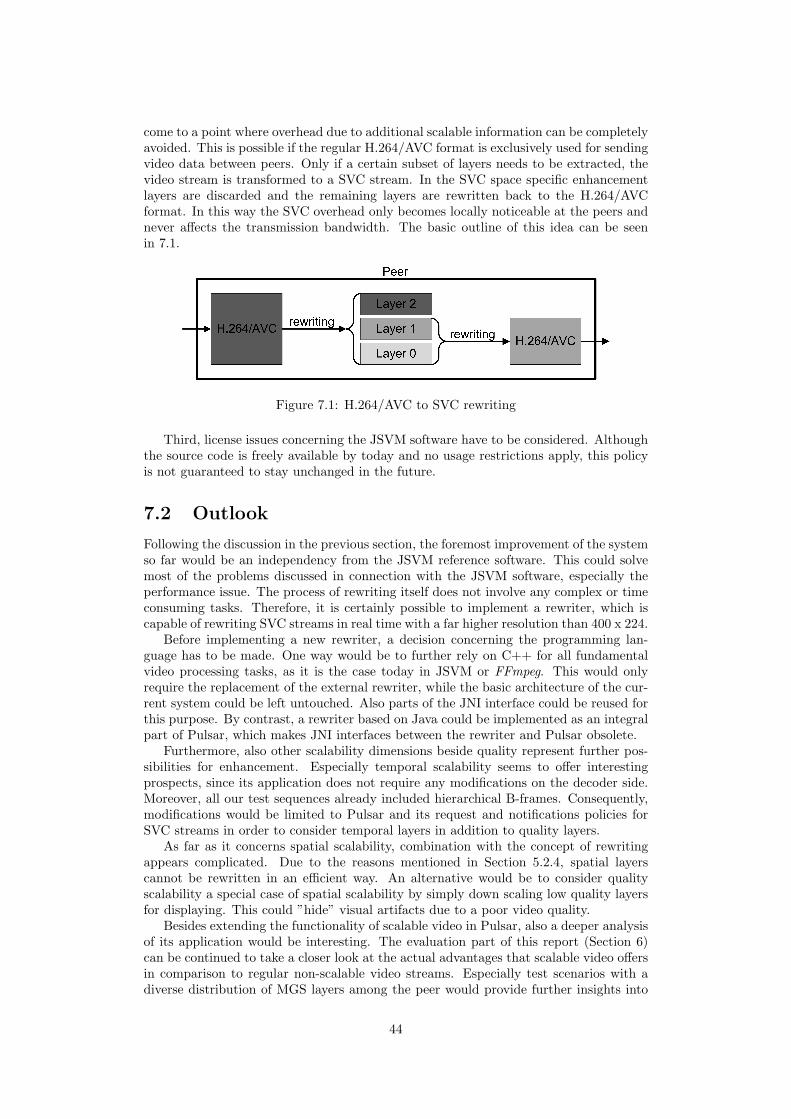
come to a point where overhead due to additional scalable information can be completelyavoided. This is possible if the regular H.264/AVC format is exclusively used for sendingvideo data between peers. Only if a certain subset of layers needs to be extracted, thevideo stream is transformed to a SVC stream. In the SVC space specific enhancementlayers are discarded and the remaining layers are rewritten back to the H.264/AVCformat. In this way the SVC overhead only becomes locally noticeable at the peers andnever affects the transmission bandwidth. The basic outline of this idea can be seenin 7.1.

Figure 7.1: H.264/AVC to SVC rewriting

Third, license issues concerning the JSVM software have to be considered. Althoughthe source code is freely available by today and no usage restrictions apply, this policyis not guaranteed to stay unchanged in the future.

7.2 Outlook

Following the discussion in the previous section, the foremost improvement of the systemso far would be an independency from the JSVM reference software. This could solvemost of the problems discussed in connection with the JSVM software, especially theperformance issue. The process of rewriting itself does not involve any complex or timeconsuming tasks. Therefore, it is certainly possible to implement a rewriter, which iscapable of rewriting SVC streams in real time with a far higher resolution than 400 x 224.

Before implementing a new rewriter, a decision concerning the programming lan-guage has to be made. One way would be to further rely on C++ for all fundamentalvideo processing tasks, as it is the case today in JSVM or FFmpeg. This would onlyrequire the replacement of the external rewriter, while the basic architecture of the cur-rent system could be left untouched. Also parts of the JNI interface could be reused forthis purpose. By contrast, a rewriter based on Java could be implemented as an integralpart of Pulsar, which makes JNI interfaces between the rewriter and Pulsar obsolete.

Furthermore, also other scalability dimensions beside quality represent further pos-sibilities for enhancement. Especially temporal scalability seems to offer interestingprospects, since its application does not require any modifications on the decoder side.Moreover, all our test sequences already included hierarchical B-frames. Consequently,modifications would be limited to Pulsar and its request and notifications policies forSVC streams in order to consider temporal layers in addition to quality layers.

As far as it concerns spatial scalability, combination with the concept of rewritingappears complicated. Due to the reasons mentioned in Section 5.2.4, spatial layerscannot be rewritten in an efficient way. An alternative would be to consider qualityscalability a special case of spatial scalability by simply down scaling low quality layersfor displaying. This could ”hide” visual artifacts due to a poor video quality.

Besides extending the functionality of scalable video in Pulsar, also a deeper analysisof its application would be interesting. The evaluation part of this report (Section 6)can be continued to take a closer look at the actual advantages that scalable video offersin comparison to regular non-scalable video streams. Especially test scenarios with adiverse distribution of MGS layers among the peer would provide further insights into

44

the performance of Pulsar using SVC. Besides the distribution of layers, as well varyingpacket sizes between the layers could influence test results. Furthermore, it would beinteresting to examine the impacts of scalable video on the bandwidth distribution andbandwidth consumption of all peers. As well, issues in the field of incentive strate-gies specifically tailored at the purpose of scalable video offer questions for additionalinvestigation.

On the protocol side of Pulsar new strategies can be tested that are specificallyadapted for the requirements of scalable video. For example various incentive strategiescan be compared in order to find the optimal assignment of payback ratios to scalablevideo layers. Furthermore, special request strategies could take into account the differentimportance of each scalable layer.

Therefore, it can be concluded that the application of scalable video in Pulsar opensup wide possibilities paired with further interesting challenges.

45

46

Bibliography

[1] Bittorrent: Offical protocol specification, Feb 2008.http://www.bittorrent.org/beps/bep_0003.html.

[2] Gnutella: Offical protocol specification, June 2008.http://www.gnutella.com.

[3] eDonkey Network: Offical Protocol Specification, June 2008.http://www.cs.huji.ac.il/labs/danss/presentations/emule.pdf.

[4] Skype: Peer-To-Peer Telephone Software, June 2008.http://www.skype.com.

[5] Kazaa media desktop: Peer-to-peer file sharing client, June 2008.http://www.kazaa.com.

[6] Limewire: Peer-to-peer file sharing client, June 2008.http://www.limewire.com.

[7] Morpheus: Peer-to-peer file sharing client, June 2008.http://www.morpheus.com.

[8] eMule: Peer-To-Peer File Sharing Client, June 2008.http://www.emule-project.net.

[9] Pulsar: Live and On-Demand Streaming Software, June 2008.http://www.getpulsar.com.

[10] Remo Meier. Peer-to-Peer Live Streaming. Master’s thesis, Swiss Federal Instituteof Technology (ETH) Zurich, July 2006.

[11] Thomas Locher, Remo Meier, Stefan Schmid, and Roger Wattenhofer. Push-to-Pull Peer-to-Peer Live Streaming. In 21st International Symposium on DistributedComputing (DISC), Lemesos, Cyprus, September 2007.

[12] H. Schwarz, T. Hinz, H. Kirchhoffer, D. Marpe, and T. Wiegand. TechnicalDescription of the HHI Proposal for SVC CE1, ISO. Technical report, IECJTC1/SC29/WG11, Document M11244, Oct 2004.

[13] H. Schwarz, D. Marpe, and T. Wiegand. Further results for the HHI Proposal oncombined scalability. ISO/IEC JTC 1/SC 29/WG 11, Oct 2004.

[14] T. Wiegand, G. Sullivan, J. Reichel, H. Schwarz, and M. Wien. Joint Draft 11 ofSVC Amendment. Joint Video Team, doc. JVTX201, Geneva, Switzerland, July,2007.

[15] H. Schwarz, D. Marpe, and T. Wiegand. Overview of the Scalable H.264/MPEG4-AVC Extension. Proc. of Int. Conf. on Image Proc.(ICIP 2006), Atlanta, GA,USA, pages 8–11, Oct. 2006.

47

[16] J. Reichel, H. Schwarz, and M. Wien. Joint Scalable Video Model (JSVM) 11, Doc.JVT-X202. Joint Video Team, Video Coding Experts Group, July 2007. http://ip.hhi.de/imagecom_G1/savce/downloads/SVC-Reference-Software.htm.

[17] M. Wien, R. Cazoulat, A. Graffunder, A. Hutter, and P. Amon. Real-Time Systemfor Adaptive Video Streaming based on SVC. Circuits and Systems for VideoTechnology, IEEE Transactions on, 17(9):1227–1237, Sept. 2007.

[18] M. Wien, H. Schwarz, and T. Oelbaum. Performance analysis of SVC. Circuitsand Systems for Video Technology, IEEE Transactions on, 17(9):1194–1203, Sept.2007.

[19] S. Wenger and T. Schierl. RTP payload for SVC. Circuits and Systems for VideoTechnology, IEEE Transactions on, 17(9):1174–1185, Sept. 2007.

[20] T. Schierl, T. Stockhammer, and T. Wiegand. Mobile Video Transmission UsingScalable Video Coding. Circuits and Systems for Video Technology, IEEE Trans-actions on, 17(9):1204–1217, Sept. 2007.

[21] VK Goyal. Multiple Description Coding: Compression meets the Network. SignalProcessing Magazine, IEEE, 18(5):74–93, 2001.

[22] Stephanos Androutsellis-Theotokis and Diomidis Spinellis. A Survey of Peer-to-Peer Content Distribution Technologies. ACM Computing Surveys, 36(4):335–371,2004.

[23] K. Lua, J. Crowcroft, M. Pias, R. Sharma, and S. Lim. A survey and comparisonof peer-to-peer overlay network schemes. Communications Surveys & Tutorials,IEEE, pages 72–93, march 2004.

[24] V.N. Padmanabhan, H.J. Wang, P.A. Chou, and K. Sripanidkulchai. Distributingstreaming media content using cooperative networking. Proceedings of the 12thinternational workshop on Network and operating systems support for digital audioand video, pages 177–186, 2002.

[25] Y. Chu, SG Rao, S. Seshan, and H. Zhang. Narada: A case for end system multicast.Selected Areas in Communications, IEEE Journal on, 20(8):1456–1471, 2002.

[26] J. Jannotti, D.K. Gifford, K.L. Johnson, M.F. Kaashoek, and J.W. O’Toole Jr.Overcast: reliable multicasting with on overlay network. Proceedings of the 4thconference on Symposium on Operating System Design, pages 14–14, 2000.

[27] PeerCast: Peer-To-Peer Broadcasting Software, June 2008.http://www.peercast.org.

[28] FreeCast: Peer-To-Peer Broadcasting Software, June 2008.http://www.freecast.org.

[29] V.N. Padmanabhan and K. Sripanidkulchai. CoopNet: The case for cooperativenetworking. Proceedings of IPTPS02, 2429:178190, 2002.

[30] M. Castro, P. Druschel, A.M. Kermarrec, A. Nandi, A. Rowstron, and A. Singh. :High-bandwidth content distribution in a cooperative environment. Proceedings ofSOSP, 2003.

[31] X. Zhang, J. Liu, B. Li, and T.S.P. Yum. CoolStreaming/DONet: A Data-DrivenOverlay Network for Efficient Live Media Streaming. Proceedings of IEEE INFO-COM, 3:13–17, 2005.

[32] N. Magharei and R. Rejaie. Understanding Mesh-based Peer-to-Peer Streaming.Proceedings of ACM NOSSDAV, 6, 2006.

48

[33] V. Pai, K. Kumar, K. Tamilmani, V. Sambamurthy, and A.E. Mohr. Chainsaw:Eliminating Trees from Overlay Multicast. Proceedings of IPTPS, pages 127–140,2005.

[34] M. Zhang, L. Zhao, J.L.Y. Tang, and S. Yang. GridMedia: A Peer-to-Peer Networkfor Streaming Multicast through the Internet. Proceedings of the ACM Multimedia,2005.

[35] Napster: Peer-to-peer music sharing client, June 2008.http://www.napster.com.

[36] CG Plaxton. Accessing Nearby Copies of Replicated Objects in a DistributedEnvironment. Theory of Computing Systems, 32(3):241–280, 1999.

[37] H. Balakrishnan, M.F. Kaashoek, D. Karger, R. Morris, and I. Stoica. Looking updata in P2P systems. Communications of the ACM, 46(2):43–48, 2003.

[38] Moni Naor and Udi Wieder. Novel architectures for P2P applications: Thecontinuous-discrete approach. ACM Trans. Algorithms, 3:34, 2007.

[39] S. Ratnasamy, P. Francis, M. Handley, R. Karp, and S. Schenker. A scalablecontent-addressable network. Proceedings of the 2001 conference on Applications,technologies, architectures, and protocols for computer communications, pages 161–172, 2001.

[40] I. Stoica, R. Morris, D. Karger, M.F. Kaashoek, and H. Balakrishnan. Chord: Ascalable peer-to-peer lookup service for internet applications. Proceedings of the2001 SIGCOMM conference, 31(4):149–160, 2001.

[41] A.I.T. Rowstron and P. Druschel. Pastry: Scalable, Decentralized Object Location,and Routing for Large-Scale Peer-to-Peer Systems. Lecture Notes In ComputerScience, 2218:329–350, 2001.

[42] B.Y. Zhao, J. Kubiatowicz, and A.D. Joseph. Tapestry: An Infrastructure forFault-Tolerant Wide-Area Location and Routing. Computer, 74, 2001.

[43] M. Mushtaq and T. Ahmed. Smooth Video Delivery for SVC Based Media Stream-ing Over P2P Networks. Consumer Communications and Networking Conference,2008. CCNC 2008. 5th IEEE, pages 447–451, 2008.

[44] P. Baccichet, T. Schierl, T. Wiegand, and B. Girod. Low-delay peer-to-peer stream-ing using scalable video coding. Packet Video 2007, pages 173–181, 2007.

[45] E. Setton, P. Baccichet, and B. Girod. Peer-to-Peer Live Multicast: A VideoPerspective. Proceedings of the IEEE INFOCOM, 96(1):25–38, 2008.

[46] M. Zink and A. Mauthe. P2P streaming using Multiple Description Coded video.Euromicro Conference, 2004. Proceedings. 30th, pages 240–247, Sept. 2004.

[47] E. Akyol, AM Tekalp, and MR Civanlar. A Flexible Multiple Description CodingFramework for Adaptive Peer-to-Peer Video Streaming. Selected Topics in SignalProcessing, IEEE Journal of, 1(2):231–245, 2007.

[48] Z. Liu, Y. Shen, S.S. Panwar, K.W. Ross, and Y. Wang. P2P Video Live Streamingwith MDC: Providing Incentives for Redistribution. Multimedia and Expo, 2007IEEE International Conference on, pages 48–51, 2007.

[49] Zattoo: Tv meets pc, June 2008.http://zattoo.com.

49

[50] J. Pouwelse, P. Garbacki, J. Wang, A. Bakker, J. Yang, and A. Iosup. Tribler:A social-based peer-to-peer system. Concurrency and Computation: Practice andExperience, 19:1–11, 2007.http://www.tribler.org.

[51] N. Zennstrm and J. Friis. Joost: P2PTV, June 2008.http://www.joost.com.

[52] TVUnetworks: P2PTV Application, June 2008.http://tvunetworks.com.

[53] PPLive: P2PTV Application, June 2008.http://www.pplive.com.

[54] M. Rabbani and R. Joshi. An overview of the JPEG 2000 still image compressionstandard. Signal Processing: Image Communication, 17(1):3–48, 2002.

[55] T. Wiegand, GJ Sullivan, G. Bjntegaard, and A. Luthra. Overview of the H.264/AVC video coding standard. Circuits and Systems for Video Technology, IEEETransactions on, 13(7):560–576, 2003.

[56] H. Schwarz, D. Marpe, and T. Wiegand. Hierarchical B-pictures. Joint Video Team,Doc. JVT-P014, Poznan, Poland, July 2005.

[57] H. Schwarz, D. Marpe, and T. Wiegand. Analysis of hierarchical B-pictures andMCTF. Proc. ICME, pages 1929–1932, 2006.

[58] C.A. Segall and G.J. Sullivan. Spatial Scalability within the H.264/AVC ScalableVideo Coding Extension. Circuits and Systems for Video Technology, IEEE Trans-actions on, 17(9):1121–1135, Sept. 2007.

[59] H. Schwarz, T. Hinz, D. Marpe, and T. Wiegand. Constrained Inter-Layer Predic-tion for Single-Loop Decoding in Spatial Scalability. Image Processing, 2005. IEEEInternational Conference on, 2:870–873, Sept. 2005.

[60] H. Schwarz, D. Marpe, and T. Wiegand. Further results on constrained inter-layerprediction. Joint Video Team, doc. JVT-O074, Busan, Korea, April, April 2005.

[61] K. Tamilmani, V. Pai, and A. Mohr. Swift: A system with incentives for trading.Second Workshop on the Economics of Peer-to-Peer Systems, 2004.

[62] S. Pateux, YK Wang, M. Hannuksela, and A. Eleftheriadis. System and Transportinterface of the emerging SVC standard. Circuits and Systems for Video Technology,IEEE Transactions on, 17(9):11491163, Sept. 2007.

[63] D. Singer, T. Rathgen, and P. Amon. File format for SVC. Circuits and Systemsfor Video Technology, IEEE Transactions on, 17(9):11741185, Sept. 2007.

[64] S. Golomb. Run-length encodings. Information Theory, IEEE Transactions on,12(3):399–401, July 1966.

[65] F. Bellard and M. Niedermayer. The FFmpeg Project, June 2008.http://ffmpeg.org.

[66] A. Segall. CE 8: SVC-to-AVC bit-stream rewriting for Coarse Grain Scalability.Joint Video Team, doc. JVT-V035, Jan. 2007.

[67] S. Liang. The Java Native Interface: Programmer’s Guide and Specification, June1999.http://java.sun.com/docs/books/jni.

50

[68] University of Hannover. Original YUV test sequences, July 2007.ftp.tnt.uni-hannover.de/pub/svc/testsequences/.

[69] Bassam Kurdali and Ton Roosendaal. Elephants Dream: Free Animation Movie,July 2007.http://orange.blender.org.

[70] HS Malvar, A. Hallapuro, M. Karczewicz, and L. Kerofsky. Low-complexity trans-form and quantization in H.264/AVC. Circuits and Systems for Video Technology,IEEE Transactions on, 13(7):598–603, 2003.

[71] J. De Cock, S. Notebaert, and R. Van de Walle. Transcoding from H.264/AVC toSVC with CGS Layers. Image Processing, ICIP IEEE International Conference on,4:73–76, Oct. 2007.

51