master in computational and mathematical engineering final...
TRANSCRIPT

!
Master In Computational and Mathematical Engineering
Final Master Project (FMP)
Influence of imbalanced datasets in the induction of Full Bayesian Classifiers
Daniel Morán Jiménez
Dr. Agusti Solanas (supervisor)
15/07/2018
Signature of the director authorizing the final delivery of the FMP:


! This work is subject to a licence of Recognition-NonCommercial- NoDerivs 3.0 Creative Commons

INDEX CARD OF THE FINAL MASTER PROJECT
Title of the FMP: Influence of imbalanced datasets in the induction of Full Bayesian Classifiers
Name of the author: Daniel Morán Jiménez
Name of the TUTOR: Dr. Agusti Solanas
Name of the PRA: Juan Alberto Rodríguez
Date of delivery (mm/aaaa): 07/2018
Degree: Ingeniería Computacional y Matemática
Area of the Final Work: Smart Health
Language of the work: English
Keywords Machine Learning, Bayesian Networks, Imbalance
Summary of the Work (maximum 250 words): With the purpose, context of application, methodology, results and conclusions of the work.
This project consists in three main tasks: first, an analysis of the current state of the art in technologies for dealing with class imbalance problems in machine learning algorithms. Second, the analysis of how this problem actually affects a particular class of statistical models, the Bayesian Classifiers, proposing solutions to the particular problems found. And third, to implement a Bayesian Classifier and develop a series of experiments that would support the assertions of the analysis, and shed more light on how this problem can be dealt with.
Abstract (in English, 250 words or less):
Machine Learning algorithms have received a growing interests in the last years with the increase in computing power and the availability of new data sources coming from digital services and a growing number of connected devices. Concerning the task of classification, one of the problems the field faces is how to deal with datasets where most of the interesting information (examples of the class or classes of interest that have to be classified) is obscured by a greater number of uninteresting examples: this is called the class imbalance problem. Much effort has been put solving this problem, either by fixing the problem modifying the dataset, modifying the particular algorithm used for the learning, or assembling different algorithms to provide imbalance-invariant assemblies.
Bayesian Classifiers are probabilistic graphical models that can be used to efficiently capture the structure of the joint probability distribution that generated a dataset. This work will analyze the impact that imbalanced datasets have in the induction of Bayesian Network models, and try to offer a way to tackle the problem directly in the algorithm, without resorting to modifying the dataset or combining algorithms.
!i

Contents1 Introduction 2
1.1 Context and justification of the Work . . . . . . . . . . . . . . . . . . . . . . . . . . . . . . . 21.2 Aims of the Work . . . . . . . . . . . . . . . . . . . . . . . . . . . . . . . . . . . . . . . . . . . 21.3 Approach and method followed . . . . . . . . . . . . . . . . . . . . . . . . . . . . . . . . . . . 21.4 Planning of the Work . . . . . . . . . . . . . . . . . . . . . . . . . . . . . . . . . . . . . . . . 31.5 Brief summary of products obtained . . . . . . . . . . . . . . . . . . . . . . . . . . . . . . . . 31.6 Brief description of the others chapters of the memory . . . . . . . . . . . . . . . . . . . . . . 4
2 Imbalanced datasets 52.1 Definition of the problem . . . . . . . . . . . . . . . . . . . . . . . . . . . . . . . . . . . . . . 52.2 Metric Selection . . . . . . . . . . . . . . . . . . . . . . . . . . . . . . . . . . . . . . . . . . . . 72.3 Interrelation with other factors . . . . . . . . . . . . . . . . . . . . . . . . . . . . . . . . . . . 8
3 State of the Art 163.1 Overview . . . . . . . . . . . . . . . . . . . . . . . . . . . . . . . . . . . . . . . . . . . . . . . 163.2 Preprocessing methods . . . . . . . . . . . . . . . . . . . . . . . . . . . . . . . . . . . . . . . . 163.3 Ensemble methods . . . . . . . . . . . . . . . . . . . . . . . . . . . . . . . . . . . . . . . . . . 253.4 Methods based on algorithm modifications . . . . . . . . . . . . . . . . . . . . . . . . . . . . . 27
4 Introduction to Bayesian Classifiers 344.1 Overview . . . . . . . . . . . . . . . . . . . . . . . . . . . . . . . . . . . . . . . . . . . . . . . 344.2 Bayesian Networks . . . . . . . . . . . . . . . . . . . . . . . . . . . . . . . . . . . . . . . . . . 344.3 The Näive Bayes Classifier . . . . . . . . . . . . . . . . . . . . . . . . . . . . . . . . . . . . . . 354.4 Structure induction in Bayesian Networks . . . . . . . . . . . . . . . . . . . . . . . . . . . . . 364.5 Parameter induction in Bayesian Networks . . . . . . . . . . . . . . . . . . . . . . . . . . . . . 384.6 Classification with Bayesian Networks . . . . . . . . . . . . . . . . . . . . . . . . . . . . . . . 40
5 Analysis of the e�ect of class imbalance in the induction of FBCs 415.1 Overview . . . . . . . . . . . . . . . . . . . . . . . . . . . . . . . . . . . . . . . . . . . . . . . 415.2 Impact of the imbalance in the structure induction . . . . . . . . . . . . . . . . . . . . . . . . 415.3 Impact of the imbalance in the parameter estimation . . . . . . . . . . . . . . . . . . . . . . . 425.4 Algorithm proposals . . . . . . . . . . . . . . . . . . . . . . . . . . . . . . . . . . . . . . . . . 46
6 Experiments 496.1 Heuristics selection . . . . . . . . . . . . . . . . . . . . . . . . . . . . . . . . . . . . . . . . . . 496.2 Impact of structure complexity in classification accuracy . . . . . . . . . . . . . . . . . . . . . 516.3 Impact of the regularization of Mutual Information in classification . . . . . . . . . . . . . . . 546.4 E�ect of the equivalent sample size and prior balance in parameter estimation . . . . . . . . . 576.5 Use of ensemble methods in imbalanced situations . . . . . . . . . . . . . . . . . . . . . . . . 576.6 Comparison with other algorithms . . . . . . . . . . . . . . . . . . . . . . . . . . . . . . . . . 576.7 Variability and zero-valued F1 metrics . . . . . . . . . . . . . . . . . . . . . . . . . . . . . . . 64
7 Conclusions 67
8 Appendix A. Classifier Implementation 68
9 Appendix B. Datasets 699.1 Real-world datasets . . . . . . . . . . . . . . . . . . . . . . . . . . . . . . . . . . . . . . . . . . 699.2 Synthetic datasets . . . . . . . . . . . . . . . . . . . . . . . . . . . . . . . . . . . . . . . . . . 69
Bibliography 71
1

1 Introduction
1.1 Context and justification of the Work
Inducing e�cient classification models for datasets with imbalanced classes is one of the multiple challenges ofmachine learning implementations. The problem of imbalance arises when the number of instances of one ofthe classes to classify (hereafter the Majority class) is clearly larger than the total number of observations ofthe opposite one (the Minority class). In this situation, the Majority class tends to be overrepresented in thepredictions of the induced clasifier. This situation can also arise in multiclass classification problems whereone or more classes overrepresented in the input data, may lead to an underrepresentation of the minorityclasses.
As a quick overview of the literature on Machine Learning will reveal, imbalanced datasets are ubiquitous inreal-life situations: examples of this can be found in several fields, from biomedical applications to sensor dataanalysis (e. g.: [1] and [2] show Smart Health applications where both fields meet). To make the situationworse, in a wide range of situations, the minority class is the class of interest, e.g.: in automated diagnosis ofan illness, there are usually hundreds of negative cases for each positive case (as most of the population isusually healthy). This makes the task of identifying and solving the class imbalance an important one, thathas been given a lot of e�ort to solve by reasearches in the field.
As we will see in the state of the art, there is no shortage of methods in the literature to deal with classimbalance. But we will also show how the class imbalance problem is more complex than a single parameterbalance, having di�erent complications depending on the particular characteristics of the dataset we areevaluating and the learning algorithm we are using. This will make more di�cult the selection of a particulartechnology, and generate a wide variance in the global results of all the algorithms used to tackle it.
Being a very wide field of study, this project will center its scope in the analysis of the impact of this problemin the induction of a particular kind of probabilistic graphical models: the Bayesian Classifiers. We will seehow this graphical models o�er some advantages over other models, by providing the analyst with a morepowerful tool that could not only be used for classification taks, but also for general inference queries, missingdata treatment, or distribution sampling. We will also see that the induction of this kind of complete modelswill come at a cost of losing some of the performance we could have achieved with other simpler but e�cientclassification-only models (e.g.: SVMs, Decision Trees or Random Forests).
1.2 Aims of the Work
Two are the main objectives of this project: first, to evaluate and validate experimentally to what extentstructure and parameter induction for Bayesian Classifiers is a�ected by the imbalance rates in reallifedatasets; and second, to propose improvements on the basic algorithms for Baysian Classifier induction inorder to overcome those induction problems. To this extent, common algorithms to cope with the imbalancedclasses problems (like preprocessing and ensembles) will be revisited, and some improvements will be proposedto try and improve over the base performance.
1.3 Approach and method followed
The first part of the project consisted in the documentation of the state of the art for both the problem ofimbalanced classes in Machine Learning, and the theory underlying Bayesian Classifiers. The former wasachieved by checking a wide set of papers on the subject, both general analysis of the problems and paperson specific solutions. A deeper understanding of the problem was achieved by implementing some of thealgorithms as part of the state of the art description. Most of the theory about Bayesian Classifiers and otherProbabilistic Graphical Models comes from [3] and [4].
The second part consisted in the implementation of a Bayesian Classifier, and the analysis of the impact ofthe class imbalance in its performance. To this extent, two possibilities where considered: the implementation
2

Figure 1: Gantt of the project showing the number of days from start and total length in days of each task
from scratch of a Bayesian Classifier ad-hoc for the project; or the modification of a stablished implementationof BCs to add the instrumentation and options required for the desired experiments. The chosen path was toimplement the BC from scratch, since the cost of understanding a reference implementation (usually morecomplex than the simple classifier required in this case) was judged to be greater than the cost of creating aprototype implementation for the experiments.
1.4 Planning of the Work
The following tasks were required to complete the work:
• D1: Documentation on the problem of class imbalance in Machine Learning. Includes the implementationof some of the algorithms, and experiments with real datasets.
• D2: Documentation on Probabilistic Graphical Models theory.• I1: Implementation of support libraries (dataset package, näive bayes reference algorithm).• I2: Implementation of the basic Full Bayesian Classifier.• A1: Analysis of the impact of the class imbalance problem in BCs (theory).• E1: Design and execution of experiments.• C1: Documentation and conclusions.
Figure 1 shows the planification of the project with the total final duration in days.
1.5 Brief summary of products obtained
Two are the main products of the project:
3

• An analysis and experiment of the impact of the class imbalance problem in the induction of BayesianClassifiers.
• And the proposal and implementation of new mechanisms to tackle the problem. Those will be addedto a Bayesian Classifier that will also be implemented as part of the project.
1.6 Brief description of the others chapters of the memory
The project is structured in the following way: Section 2 shows a brief introduction to the topic of learningin imbalanced datasets; Section 3 shows the most frequent solutions in the literature for the problem ofimbalanced datasets; Section 4 gives a brief introduction to Bayesian Classifiers and motivates their selectionas the classifiers to study; Section 5 analyzes the expected influence of the class imbalance from a theoreticalperspective; Section 6 describes the experiments that were conducted in order to validate some of theassumptions in section 5, and analyzes their results; finally, Section 7 summarizes the conclusions and futurework. Extra information about the implementation details, statistical analysis and the datasets used alongthe document can be found in the apendices.
4

2 Imbalanced datasets
2.1 Definition of the problem
2.1.1 Definition of Learning
The first step on defining the problem will be to make a brief introduction to the concept of learning, tointroduce terms and notation that will be used across the rest of this document (a more formal introductioncan be found in [3]).
Informally, the task of learning will consist in generating a model that captures the underlying structure of aproblem, given a limited amount of examples; the limited number of examples will make the induced modeljust an approximation, that we will hope to be accurate enough for our purposes.
Formally, the learning task will consist on:
• given a dataset D = {X[1], X[2]..X[M ]} consisting of M examples drawn from an underlying, probablyunknown distribution, P ú(X),
• where each X consists of a set of N variables, X1, X2, ...XM ,
• and where each variable has its own domain Xi œ V al(Xi) (that may be discrete, in which caseV al(Xi) = {r1, ..., rk}),
inferring a model M that captures the structure of the original distribution, so that:
PD(X) ¥ P ú(X)
This adopt this definition based on probability theory, as we will see that it generalizes to types of learningwhere the output may not be a probability.
There are multiple tasks that can be accomplished through learning. This tasks can be divided attending todi�erent criteria. Considering the goal distribution, we can distinguish two kind of tasks:
• generative learning: where the objective of the learning is to discover the full structure of the under-lying distribution, so the target probability distribution is PD(X1, X2, ....XN ) ¥ P ú(X1, X2, ....XN ).
• discriminative learning: where the objective of learning is to discover the conditional dis-tribution over one of the variables, so the target distribution is PD(X1, X2, ..Xi|Xi+1..XN ) ¥P ú(X1, X2, ..Xi|Xi+1..XN ).
Generative learning models, like Bayesian Classifiers, are more general than discriminative ones, in the sensethat, providing a full joint distribution, they also provide a way of getting the conditional one (while theopposite is usually not true).
Learning algorithms can also be divided according to their train objectives in supervised and unsupervised.In the case of supervised learning, the dataset D = {< Xi, yi >}
i=1..Mis a set of example tuples containing
a list of values for the predictor variables and a value for the target class (or classes), that will be used toinferr a model of the conditional probability of the target class on the predictions. The problem can then bespecified as a search for the model that best captures the true distribution P ú(Y |X1, X2, ...XM ).
In unsupervised learning, the objective is, once again, to infer a variable (or set of variables) from thegiven data, but in this case, the dataset contains no information about the target classes. The rest of thepaper we will focus mostly on supervised classification problems.
The learning process can be viewed as an optimization process where a target loss function is minimized forthe dataset instances. A loss function gives an estimate of how well a model fits the data represented by agiven dataset D. Commonly used loss functions include the classification error :
5

Er = E(x,y)≥P̃[I {hP̃(x) ”= y}]
where hP̃
(x) is our estimation function; i.e.: the probability of selecting the wrong label, given the trainingdata. Another commonly used loss function, that takes into account the uncertainty in the prediction is theconditional log-likelihood:
L = E(x,y)≥P ú#log P̃ (y|x)
$
The selection of the loss function to optimize will influence the behavior of our classifier when dealing withimbalanced datasets, as we will show in subsequent sections.
2.1.2 Model selection
The learning process involves the choice of a representation for the induced model. This choice of representationwill determine how rich the hypothesis space will be, and this decision will have an impact in the ability ofthe model to generalize. As the model gets more complex, and the hypothesis space wider, the capacity forthe model to accurately represent the target distribution grows higher. But there is a caveat to this increasedcomplexity. Since the amount of dataset instances is limited, as the hypothesis space grows, the density ofexamples shrinks, and so the posterior probability of unseen examples tend to zero. These low probabilitiesand high number of possible models make the task of selecting the most appropriate one (the one that betterfits to the target unknown distribution) more di�cult. This problem is referred to as the variance. A reachspace of hypothesis can also lead to a phenomenon called overfitting, where the classifier learns to perfectlypredict the training set, while losing its ability to generalize to other unseen data.
On the contrary, when the hypothesis space is so small that the target probability distribution can’t beadequately fit, it’s said that the model has a high bias. There is a necessary tradeo� between bias andvariance in model designing; this tradeo� will usually be dealt with by introducing special regularizationterms in the loss function expression.
Since the objective of the learning task is usually to perform classification or inference over new instances, weneed a way of estimating its generalization ability. This evaluation involves calculating some kind of metricover a set of instances, but drawing them from the training data will not give a good estimation over unseeninstances. In order to get an unbiased estimation of the generaliation ability of a model, a subset of theavailable dataset instances will be hold out, to create a test dataset. The remaining data will be referred toas the training dataset. For those cases that imply model selection (whether it is a hyperparameter searchor a selection among a set of algorithms), this training dataset can be in turn splitted, to form a third split,called validation dataset that will be used to calculate the metrics that will be used in the model selectionprocess.
2.1.3 Data imbalance
The problem of data imbalance is defined as the scenario where, given a dataset D = {< Xi, yi >}i=1..M
,where the target variable has K di�erent classes, y1, ..yk and :
÷i, j s.t. MD[yi] << MD[yj ]
where MD[yi] is the number of times the value yi appears in dataset D. Hereafter, for the binary cases, theunderrepresented class will be called minority or positive class, while the overrepresented one will be calledmajority or negative. This situation usually leads to an understimation of the probability of yi, that maybe harmful for our objectives in two ways:
6

• since the available dataset instances are usually very scarce when compared with the complete featurespace, it may be the case that the empirical distribution of examples in the dataset may not reflectappropriately the underlying distribution.
• most of the times, accurately predicting the positive class is the target of our modelling, so classificationerrors will not be as important for the negative class as it would be for the positive (i.e.: underrepresentingthe positive class is more harmful than doing the same for the negative one).
As we will see in section about interrelation with other factors, the class imbalance problem is usually mixedwith other factors in practice, that may change the extent of its impact on the learning process.
2.2 Metric Selection
The inability of the classical classifiers to cope with imbalance problems is largely due to the loss functionthey are designed to optimize, as pointed out in [5]. Most classifiers are trained to optimze the 0-1 loss, thatcan be understood as 1 minus the Accuracy, a global measure that doesn’t take into account the per-classclassification errors. Both performance metrics have a strong bias towards the majority class, to the pointthat, for highly imbalance cases, the simplest strategy of always predicting the majority class will o�er areally high Accuracy. This is highly problematic in most cases, as it is usually the case that the minorityclass classification accuracy is more important than the majority one (e.g.: in automated diagnosis systemswhere patients with an actual disease represent the minority class).
Classification error is usually defined in terms of the confusion matrix: a K ◊ K matrix, C (where K is thenumber of classes) that indicates, for any element ci,j , the number of elements of the class Ki classified aselements of Kj . Two local performance measures are particularly important in this context:
• The precision measures, out of the total number of ground truth instances of a particular class, howmany of them where correctly classified. It’s defined with the following formula for the multiclass case:
Pi = ciiqK
j=1 cji
• The recall measures the amount of instances classified as being part of a particular class, from thetotal number of instances of that class in the ground truth distribution. It’s defined with the followingformula for the multiclass case:
Ri = ciiqK
j=1 cij
This two local measures serve as building blocks for other global metrics that have di�erent properties whendealing with accuracy. Most of those metrics can be redefined as particular instances of the weighted Höldermeans across class recalls. The following list shows the most common ones in the literature:
• The a-mean is the arithmetic mean among recalls, i.e.:
A =Kÿ
i=1
1K
Ri
• The g-mean is the geometric mean among recalls, i.e.:
A = K
ı̂ıÙKŸ
i=1Ri
7

Another common metric in the literature is the F 1 metric, defined as the harmonic mean of precision andrecall:
F 1i
= 2 Pi · Ri
Pi + Ri
This metric, that gives the same weight to both Precision and Recall, is an instance of the more general classof F — metrics defined as:
F —
i= (1 + —2) Pi · Ri
—2Pi + Ri
It’s important to highlight here that, in most cases, the importance of Precision and Recall for a particularproblem may not be equal, as there may be very di�erent misclassification costs for the positive classes(medical diagnosis is a common example). For those cases, the F — metric o�ers a tool to select the desiredlevel of significance of both components.
The total error classification Accuracy can also be defined in terms of the elements of the confusion matrix, asthe total number of elements correctly classified (the diagonal of the confusion matrix) over the total numberof elements:
Acc =q
K
i=1 ciiqK
j,i=1 cij
For those cases where the classifier gives as output a continous value, that can be interpreted as the certaintyof the classification as the possitive example (in a two-class scenario), another commonly used measure isbased on the Receiver Operating Characteristic curve (ROC curve). This is a curve plotting true positiverate against false positive rate, for each value of the threshold (so that a curve that pass through the upperleft corner corresponds to a perfect classifier and a curve that goes along the lower-left upper-right cornersdiagonal behaves as a random classifier). The total Area Under the Curve (AUC) is a metric in the [0, 1]interval that has been proved to be useful in imbalanced scenarios.
It’s important to highlight that there is no metric that can be selected as the optimal classification metric forall datasets and classifiers. For instance, in its study of the e�ect of several hybrid algorithms, [6] shows thatmetric selection can have an important impact in classifier rankings for the same datasets, making di�cult todecide which classifier is optimal for a given problem. To account for that di�culty, the experimental part ofthis work will show the results for di�erent metrics, trying to capture both their strengths and weaknesses.The set of metrics will usually contain: Accuracy, F1, Precision and Recall. Area Under the Roc Curve(AUC) analysis will also be used in the final algorithm comparisons.
2.3 Interrelation with other factors
The imbalance of datasets alone can’t explain the di�culties in finding a good predictive model for thetarget datasets, and many papers even point out that the fall in performance observed in some imbalanceddatasets may not be due to the imbalance itself, but to other factors that are most commonly found when ahigh degree of imbalance is present. This can be inferred from the fact that datasets with the same level ofimbalance may have very di�erent classification complexities [7]. The following subsections describe severalfactors that influence the di�culties in classification learning with a particular dataset.
2.3.1 Interclass imbalance
Even if the proportion of the two classes is globally balanced, a single class might have most of its observationsgrouped in a single cluster, while other smaller clusters get infrarrepresented, so becoming harder to classify
8

7 8 9
4 5 6
1 2 3
−1 0 1 2 −2 −1 0 1 2 −2 −1 0 1 2
−2 −1 0 1 −2 −1 0 1 2 −2 −1 0 1
−2 −1 0 1 2 −1 0 1 2 −2 −1 0 1 2−2
−1
0
1
2
−2
−1
0
1
−2
−1
0
1
−2
−1
0
1
2
−2
−1
0
1
2
−2
−1
0
1
2
−2
−1
0
1
2
−2
−1
0
1
−2
−1
0
1
2
x
y
classnegative
positive
Figure 2: Dataset with growing interclass imbalance
(a problem usually called of the “small (hidden) disjuncts”, in the literature). The number and relative sizes ofthe di�erent class disjunts can be one of the factors of the classification di�culty [8], [9]. Di�erences in hubnessfor the classes may also a�ect the way imbalance a�ects, even to the point of producing misclassificationof the majority class in favor of the minority, when small disjuncts of the majority class appear in a regionwhere there is a bigger density of minority class examples[10], [11].
Figure 2 shows a set of datasets with two classes, each one composed by eight clusters, with an 0.1 imbalancerate, but with a di�erent value of interclass imbalance for the possitive class. Interclass imbalance is markedwith a number from 1 to 9. Appendix B explains the formula used to calculate the number of examples ineach disjunct based on its disjunct degree.
As we can see, as the interclass imbalance grows, most of the examples concentrate in a small number ofdisjuncts, to the point where really small disjuncts can be disregarded as noise.
Figure 3 shows the e�ect of the interclass imbalance level (with all the other parameters fixed) in the Accuracy,F1, Precision and Recall classification metrics for a C5.0 classification tree. As we can see in the graph, theglobal metrics seem to improve as the global class imbalance grows. This e�ect comes from the increaseddensity of one of the disjuncts with respect to the rest: as the density on the biggest disjunct grows, so dothe classifier performance for that disjunct; and since the positive class examples concentrate in that disjuntas the interclass imbalance grows, the percentage of appropriately classified examples also grows.
Figure 4 shows how the errors committed by the model concentrate in the small disjuncts, making the recallfor those disjuncts a lot higher than the one of the biggest possitive class disjunct, that is perfectly captured
9

0.00
0.25
0.50
0.75
1.00
2.5 5.0 7.5disjuncts
value
metricacc
F1
Precision
Recall
Figure 3: E�ect of the imbalance level in the classification for C5.0 classification trees
by the model.
2.3.2 Complexity of the classification borders
With independence of the balance between classes, the complexity of the function that defines the classificationborder influences the expected learnt accuracy (e.g.: a linear classification border will be very easy to beinduced from examples, without any regard to the balance between classes) [12].
Figure 5 shows a group of datasets generated in growing degree of complexity. As it is described in thedataset appendix, complexity will be represented by a di�erent number of clusters for each class.
Figure 6 shows the e�ect of the growing complexity level (with all the other parameters fixed) in the Accuracy,F1, Precision and Recall metrics for C5.0 classification trees. As we can see, the metrics that depend on theperformance of the positive class or both classes, rapidly decay as the complexity of the dataset increases,while those dependant on the global number of errors remain higher (as most of the examples are still correctlyclassified; the negative ones, mostly).
2.3.3 Size of the training set
Imbalance between classes usually pose a smaller threat on bigger datasets, where even if the Minor classcontains relatively less observations, it contains enough in absolute value to clearly define the classificationborders [12]. Conversely, when the number of instances in the dataset is very low, the induction algorithmhas a lack of information about the boundaries of the problem, so making it more di�cult to generalize [11].This problems may in time be considered as instances of other data intrinsic problems, as the small hiddendisjuncts or the presence of noise.
Figure 7 shows a group of datasets generated with exponentially growing size (all other parameters keptequal).
Figure 8 shows the e�ect of the dataset size with an imbalanced dataset (with all the other parameters fixed)in the Accuracy, F1, Precision and Recall metrics for C5.0 classification trees (size is in log scale). Thegraphic shows how all metrics usually improve as the size of the dataset grows, achieving high recalls in the
10

−2
−1
0
1
2
−2 −1 0 1x
y
classnegative
positive
Figure 4: Errors committed in classification with high interclass imbalance
positive class for big sizes, while mantaining the high imbalance rate. These figures show how the imbalanceproblem is usually confined to the realm of small to medium size datasets.
2.3.4 Level of noise or overlap between classes
Even if the border to be induced has an easy expression, a high level of noise or a clear overlap betweenclasses may make learning the target function a really di�cult task. In fact, some authors point out that, forbig enough datasets, the e�ect of imbalance is negligible with respect to the e�ect of class overlap [13] whenconsidered independently (although the performance loss is higher than the expected combined loss whenboth are present).
Figure 9 shows a group of datasets generated with exponentially growing level of overlap (all other parameterskept equal). As we can see, as the overlap level increases, the borders between disjuncts become more fuzzy,and it gets progresively more di�cult to properly assign a region to each disjunct. This grade of overlapwould force a classifier algorithm to return a highly complex model (to account for all the small di�erences ina very complicated border) or to rely on a statistical approximation (that would give a lower certainty as thelevel of overlap grows).
Figure 10 shows the e�ect of the dataset overlap (with all the other parameters fixed) in the Accuracy, F1,Precision and Recall metrics for C5.0 classification trees.
[13] o�ers one explanation on the concrete mechanism for the classification loss due to the mixture of overlapand imbalance in their study of the complexity of the induced classifier (measured in this case with the numberof support vectors in a SVM trained in the dataset) for di�erent datasets. Their results show that increasinglevels of overlap, or combined imbalance and overlap, forces the classifier to retain more examples as supportvectors, thus increasing the complexity of the classifier. Interestingly enough, this e�ect is not present in thedatasets with high imbalance and low overlap. These results show that an increased complexity may be one
11

7 8 9
4 5 6
1 2 3
−1 0 1 −1 0 1 −1 0 1
−2 −1 0 1 2 −2 −1 0 1 2 −2 −1 0 1 2
−2 0 2 −2 −1 0 1 2 −2 −1 0 1 2−2−1012
−2
−1
0
1
2
−1
0
1
−2
−1
0
1
2
−2
−1
0
1
2
−1
0
1
−2
0
2
−1
0
1
2
−1
0
1
2
x
y
classnegative
positive
Figure 5: Dataset with growing concept complexity
0.25
0.50
0.75
1.00
2 4 6 8complexity
value
metricacc
F1
Precision
Recall
Figure 6: E�ect of the complexity level in the classification for C5.0 classification trees
12

7 8 9
4 5 6
1 2 3
−2 −1 0 1 2 −2 −1 0 1 2 −2 −1 0 1 2
−2 −1 0 1 2 −2 −1 0 1 2 −2 −1 0 1 2
−1 0 1 −1 0 1 −1 0 1 2
−1
0
1
2
−2
−1
0
1
2
−2
−1
0
1
2
−1
0
1
−2
−1
0
1
−2
−1
0
1
2
−2
−1
0
1
−1
0
1
2
−2
−1
0
1
2
x
y
classnegative
positive
Figure 7: Dataset with growing size
0.25
0.50
0.75
1000 10000size
value
metricacc
F1
Precision
Recall
Figure 8: E�ect of the dataset size in the classification for C5.0 classification trees
13

4 5 6
1 2 3
−2 −1 0 1 2 −2 −1 0 1 2 −2 −1 0 1 2 3
−1 0 1 −1 0 1 2 −2 −1 0 1
−2−1012
−2
0
2
−2−1012
−2−1012
−2−101
−2−1012
x
y
classnegative
positive
Figure 9: Dataset with growing level of overlap
0.00
0.25
0.50
0.75
1 2 3 4 5overlap
value
metricacc
F1
Precision
Recall
Figure 10: E�ect of the dataset size in the classification for C5.0 classification trees
14

of the factors that reduces the expected average performance in these kinds of datasets: algorithms that failto generate a complex enough classifier may fail to adequately separate the classes.
15

3 State of the Art
3.1 Overview
A lot of reasearch e�ort has been devoted to diminishing the e�ects of class imbalance in machine learningproblems. Most common methods can be grouped in the following categories:
• Preprocesing methods, sampling methods being the most popular, that expect to solve the accuracyproblem by modifying the datasets, improving the balance between classes (by removing examples ofthe majority class, or replicating or synthesizing new ones of the minority one) or removing examplesthat make learning particularly di�cult (like borderline examples). Here is important to note thatthe optimal class distribution for a given problem may not be the balanced classes (unless perfectlybalanced classes have proven to be usually a good aproximation of the optimal), but a distribution withsome skew, that will depend on the classifier and the dataset characteristics. This fact complicates thetask of selecting the appropriate preprocessing method and level.
• Methods based on new algorithms, designed specifically with the avoidance of the class imbalance inmind. It’s worth mentioning here that di�erent algorithms present di�erent levels of performance inhigh imbalance scenarios (e.g.: SVMs perform far better than decision trees, that are more commonlyfound in the imbalance literature).
• Methods based in Ensembles of algorithms that combine multiple algorithms or preprocesingtechniques for improving the combined accuracy.
• Weighted learning methods, that modify the learning algorithm to take into higher considerationexamples of the minority class than those in the majority class (as they are usually more important,anyway). Weighting methods will usually be part of ensemble algorithms or will require the modificationof existing algorithms to work (and so we will study them as part of those categories).
• In the last years, some Feature selection methods have also appeared, specially for high dimensionaldata, that try to overcome the imbalance problems by selecting a subset of the dataset features overwhich the classifier behaves better (e.g.: [14]).
The next sections o�er an overview of some of the most popular examples provided by the literature for eachcategory, along with a brief description and comparison.
3.2 Preprocessing methods
3.2.1 Evaluation of the preprocessing methods
In order to evaluate the performance of the preprocessing methods in the task of reducing the impact of theimbalance in classification tasks, we will apply them to both real and synthetic datasets first, and then we willapply four di�erent classifiers to the resulting datasets to evaluate the joint performance. We selected fourdi�erent types of classifiers to better address the di�erent e�ciency that particular preprocessing methodscould have on di�erent classifier types. All classifier implementations belong to R’s Caret package [15], thatcompiles di�erent popular machine learning libraries. All examples are trained with a 5-fold Cross Validationto estimate the final metaparameters. The selected classifiers are the following:
• A decission tree algorithm, C5.0 (from the C5.0 caret package).• A Random Forest algorithm (from the ranger caret package).• A Bayesian Generalized Linear Model (from the bayesglm caret package).• A Suppport Vector Machine with Radial Kernel (from the svmRadial caret package).
16
3.2.2 Random sampling methods
The most simple type of preprocessing methods are Random Undersampling (RUS) and Random Oversamp-pling (ROS). RUS consists in removing random elements from the majority class in the dataset, until bothclasses are balanced (or from many classes until a global class balance is achieved in multiclass problems).ROS, on the other hand, consists in replicating random elements of the minority class set, until the totalnumber of elements in both sets are roughly equal.
These simple methods are really easy to implement but o�er a poor performance. Each of them has alsoits particular disadvantages: by replicating existing instances without adding new information, ROS makesthe dataset more prone to overfitting; on the other hand, by removing random instances, RUS wastes theinformation contained in those instances, that may be potentially valuable for classification.
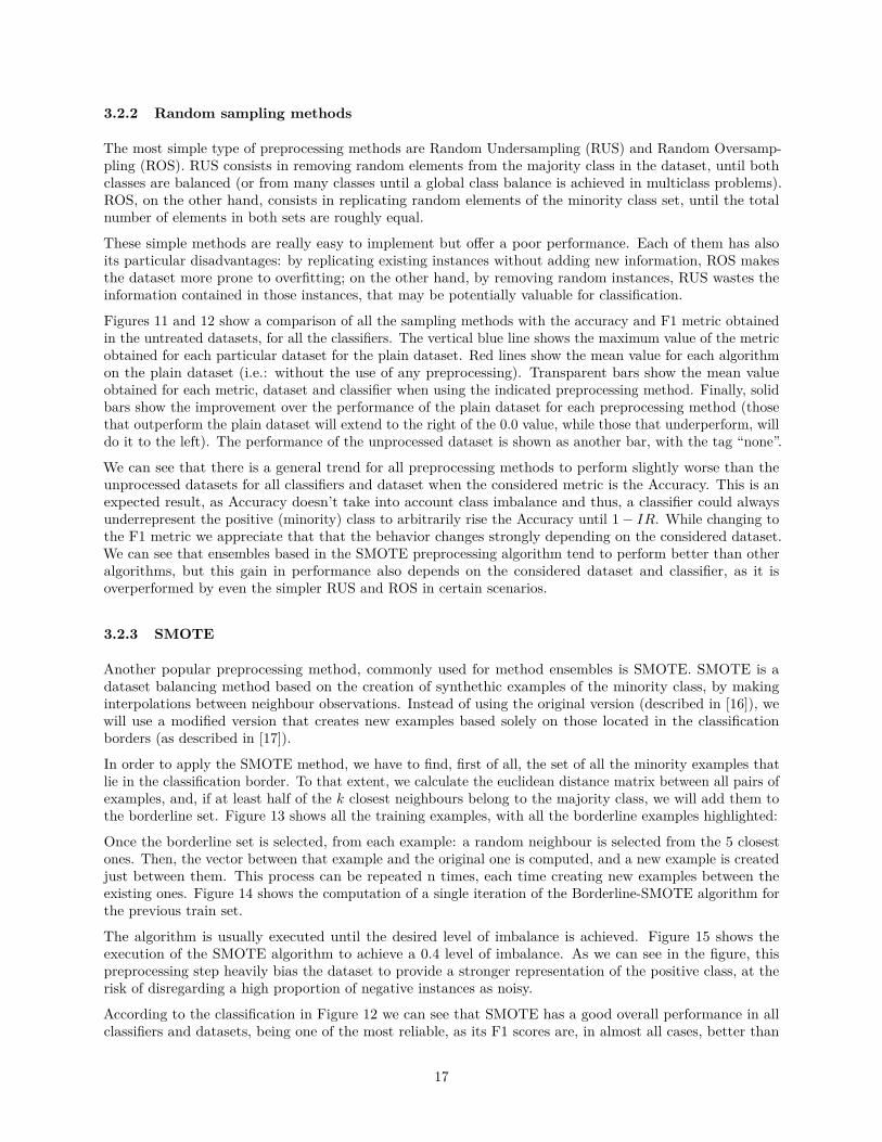
Figures 11 and 12 show a comparison of all the sampling methods with the accuracy and F1 metric obtainedin the untreated datasets, for all the classifiers. The vertical blue line shows the maximum value of the metricobtained for each particular dataset for the plain dataset. Red lines show the mean value for each algorithmon the plain dataset (i.e.: without the use of any preprocessing). Transparent bars show the mean valueobtained for each metric, dataset and classifier when using the indicated preprocessing method. Finally, solidbars show the improvement over the performance of the plain dataset for each preprocessing method (thosethat outperform the plain dataset will extend to the right of the 0.0 value, while those that underperform, willdo it to the left). The performance of the unprocessed dataset is shown as another bar, with the tag “none”.
We can see that there is a general trend for all preprocessing methods to perform slightly worse than theunprocessed datasets for all classifiers and dataset when the considered metric is the Accuracy. This is anexpected result, as Accuracy doesn’t take into account class imbalance and thus, a classifier could alwaysunderrepresent the positive (minority) class to arbitrarily rise the Accuracy until 1 ≠ IR. While changing tothe F1 metric we appreciate that that the behavior changes strongly depending on the considered dataset.We can see that ensembles based in the SMOTE preprocessing algorithm tend to perform better than otheralgorithms, but this gain in performance also depends on the considered dataset and classifier, as it isoverperformed by even the simpler RUS and ROS in certain scenarios.
3.2.3 SMOTE
Another popular preprocessing method, commonly used for method ensembles is SMOTE. SMOTE is adataset balancing method based on the creation of synthethic examples of the minority class, by makinginterpolations between neighbour observations. Instead of using the original version (described in [16]), wewill use a modified version that creates new examples based solely on those located in the classificationborders (as described in [17]).
In order to apply the SMOTE method, we have to find, first of all, the set of all the minority examples thatlie in the classification border. To that extent, we calculate the euclidean distance matrix between all pairs ofexamples, and, if at least half of the k closest neighbours belong to the majority class, we will add them tothe borderline set. Figure 13 shows all the training examples, with all the borderline examples highlighted:
Once the borderline set is selected, from each example: a random neighbour is selected from the 5 closestones. Then, the vector between that example and the original one is computed, and a new example is createdjust between them. This process can be repeated n times, each time creating new examples between theexisting ones. Figure 14 shows the computation of a single iteration of the Borderline-SMOTE algorithm forthe previous train set.
The algorithm is usually executed until the desired level of imbalance is achieved. Figure 15 shows theexecution of the SMOTE algorithm to achieve a 0.4 level of imbalance. As we can see in the figure, thispreprocessing step heavily bias the dataset to provide a stronger representation of the positive class, at therisk of disregarding a high proportion of negative instances as noisy.
According to the classification in Figure 12 we can see that SMOTE has a good overall performance in allclassifiers and datasets, being one of the most reliable, as its F1 scores are, in almost all cases, better than
17

yeast
ecoli sick wdbc
Abalone allhypo allrep
0.0 0.4 0.8
0.0 0.4 0.8 0.0 0.4 0.8
Bayes GLM
C5.0
Radial SVM
Random Forest
Bayes GLM
C5.0
Radial SVM
Random Forest
Bayes GLM
C5.0
Radial SVM
Random Forest
Accuracy
nam
e
preprocessingcnn
none
oss
ros
rus
smote
smote_tomek
tomek
Figure 11: Comparative of random sampling methods using Accuracy metric
18
yeast
ecoli sick wdbc
Abalone allhypo allrep
−0.5 0.0 0.5 1.0
−0.5 0.0 0.5 1.0 −0.5 0.0 0.5 1.0
Bayes GLM
C5.0
Radial SVM
Random Forest
Bayes GLM
C5.0
Radial SVM
Random Forest
Bayes GLM
C5.0
Radial SVM
Random Forest
F1
nam
e
preprocessingcnn
none
oss
ros
rus
smote
smote_tomek
tomek
Figure 12: Comparative of random sampling methods using F1 metric
19

−3
−2
−1
0
1
2
3
−4 −2 0 2x
y
classnegative
positive
Figure 13: Highlighted borderline instances
−3
−2
−1
0
1
2
3
−4 −2 0 2x
y
classnegative
positive
Figure 14: Examples synthesized by the SMOTE Algorithm
20

−3
−2
−1
0
1
2
3
−4 −2 0 2x
y
classnegative
positive
Figure 15: Execution of the SMOTE algorithm for a 0.4 level of imbalance
those of the plain datasets (unlike other methods that exhibit a worse behavior depending on the classifierand dataset).
3.2.4 Tomek Links
Tomek links are pairs of observations each one belonging to a di�erent class such that they are also the nearestneighbours in the complete dataset, i.e.: let d(·, ·) be a metric distance, and P = (xmin, xmaj) a pair ofexamples, one belonging to the minority class (xmin) and the other one belonging to the majority class (xmaj),if there is no other observation xk such that d(xk, xmaj) < d(xmin, xmaj) or d(xk, xmin) < d(xmin, xmaj)then P is a Tomek Link. According to this definition, each member of a Tomek link has to be either part ofthe classification border or classification noise [18].
Figure 16 shows the training examples with the highligted Tomek links, and Figure 17 the resulting datasetonce three iterations of the Tomek Links algorithm have been executed.
Directly removing the negative example of each Tomek Link should improve the classification border by twomeans: removing the noise in the minority class and creating a more defined classification border.
Returning to the classification on Figure 12, we find that, when used in isolation, its e�ect is usually lowcompared to that of other more performant techniques (like RUS or SMOTE). It will appear, though, insome of the ensemble preprocessing methods.
3.2.5 Condensed Nearest Neighbours rule
The Condensed Nearest Neighbours algorithm was born as a mechanism to create a minimum set ofclassification examples for the Nearest Neighbour classification algorithm. It works incrementally, constructing
21

−3
−2
−1
0
1
2
3
−4 −2 0 2x
y
classnegative
positive
Figure 16: Highlighted tomek links
−3
−2
−1
0
1
2
3
−4 −2 0 2x
y
classnegative
positive
Figure 17: Example dataset with Tomek Links removed
22

−3
−2
−1
0
1
2
3
−4 −2 0 2x
y
classnegative
positive
Figure 18: CNN Rule applied to the example dataset
a reference set, Store with the following rule: for each example, use the Nearest Neighbour algorithm over theStore set to classify the example; if it’s correctly classified, the example is put in the discard set, Grabbag,otherwise, it is added to the Store set. The algorithm continues until all the examples are in one of the twostores. Then, it continues adding examples from the Grabbag set, until the later is empty, or a full iterationover the set has been completed without adding any element to the Store set. The Store set is then the targetclean dataset.
Globally, the algorithm will tend to remove redundant examples that are located far from the classificationboundaries, thus theorically decreasing the total size of the dataset to be processed, without hamperingmuch the classification accuracy. This reduction has two benefits: being a reduction in redundant examples,it should make the classification boundaries clearer; and the reduction make the training stage easier incomputational terms. Figure 18 shows the testing dataset once cleaned with the CNN rule (overimposed overthe shaded original dataset).
Figure 12 shows that this method has the worse performance of all the studied methods, usually performingworse than the plain dataset would. It is anyway used in some of the most popular ensemble methods.
3.2.6 Ensemble preprocessing methods
Imbalance literature o�ers examples of multiple preprocessing proposals that consists in a combination ofother baseline preprocessing techniques. The following ones will be used as a representative set:
• One Side Selection [19]: this approach consists in a combined use of Tomek Links to remove borderlineand noisy examples, followed by the CNN rule to remove the redundant ones. Figure 19 shows anexample of application of One Side Selection to the example dataset.
• Smote + Tomek Links (taken from the review in [20]): in this case, both classes are removed from
23

−1
0
1
2
−2 −1 0x
y
classnegative
positive
Figure 19: One side selection example
the Tomek Links, in order to clean noisy minority class examples that may invade the majority classwhile oversampling. Figure 20 shows an example of application of Smote + Tomek to the exampledataset.
3.2.7 Current criticism with resampling methods
Despite its widespread use in the imbalanced learning domain, resampling methods have received somecriticism in the last years (see [21], for instance). Some of the problems inherent to this methods are:
• Concerning the character of the dataset, resampling don’t really add any new information to it, andit can even remove it (as is the case of undersampling methods). Even in the case of the syntheticgeneration of examples, no new information is generated.
• As they generate no new information, resampling methods have to choose between oversampling (withexisting or synthetic data, based in the existing one), that can lead to overfitting; or balancing byremoving, that discard potentially useful information.
• There is usually no theoretically sound reason to select a particular class balance level for a givendataset. Equally balanced classes are usually chosen as they tend to o�er an acceptable performance;other approaches may search for an appropriate imbalance level in an empirical way, through crossvalidation, as another metaparameter.
• In any case, the goal of data balancing is to explicitly deviate from the underlying distribution in orderto favor learning with current classifier induction algorithms. This objective works against one of thepossible objectives of learning, that is the induction of a model of the true underlying distribution fromwhich the dataset has been drawn.
24

−3
−2
−1
0
1
2
3
−4 −2 0 2x
y
classnegative
positive
Figure 20: Smote+Tomek example
Critics of the sampling methods argue that those methods are only useful because they help us in usingwell stablished skew-sensitive algorithms with highly imbalanced data; for those cases, the developmentof skew-insensitive algorithms would render the sampling methods useless, reducing the complexity of theproblem.
3.3 Ensemble methods
In the section about preprocessing methods we’ve already seen preprocessing ensemble methods, that combinedtwo di�erent preprocessing methods to obtain a better one. In the last years, similar approaches have appearedthat combine preprocessing methods with ensemble algorithms. The goal of ensemble algorithms is to o�era way to combine di�erent weak classifiers in order to create a combined algorithm with a performancethat is greater than that of any of its components. This improvement will be possible as long as the basealgorithms that compose the ensemble have better performance than the simple chance, and are diverse, i.e.:that di�erent base algorithms make di�erent kinds of errors, given the same data. In order for the latterrequirement to be accomplished, algorithms are required to be weak, i.e.: algorithms whose performancegreatly vary with di�erences in data (that is, classifiers with high variance). Ensemble algorithms are mostcommonly used with multiple trained instances of the same base classification weak algorithm.
The two most widely used families of algorithms are boosting and bagging. In bagging, multiple datasetsare created from the original one, by sampling with replacement, so each algorithm of the ensemble issimultaneusly trained with slightly di�erent datasets (this di�erence will allow for the diversity of the basealgorithms). Once all algorithms are trained, the class of an example is determined by majority vote amongthem. In the case of boosting the algorithms are trained sequentially, so the results of the first classifiers areused to guide the training of the subsequent ones. This is normally achieved by giving di�erent weights tothe misclassified examples, so later classifiers get specialized in di�cult examples.
25

When it comes to design solutions using ensembles to address the class imbalance problem, multiple approachescan be found in the literature. Following the taxonomy in [22], we will divide them in the following classes:
• Boosting-based: approaches that make use of boosting along with some preprocessing mechanisms.Examples of this category are RUSBoost and SMOTEBoost.
• Bagging-based: approaches that combine bagging with preprocessing are usually simpler than boosting-based, as they don’t have to modify the original algorithm to apply preprocessing. Some examples areOverBagging, UnderBagging or SmoteBagging.
• Cost-sensitive Boosting: some boosting algorithms can be modified so that the weights they use totrain later classifiers are modified based on the class imbalance. Most of the classifiers in this categoryare modifications of the classical Adaboost algorithm. Some examples are RareCost or AdaC2 ([23]).
• Hybrid ensembles: that is, those that combine boosting with bagging. E.g.: EasyEnsemble andBalanceCascade [24]
In the following sections we will present one example of each of this categories. We will select the examplesamong the most performant ones for its category, as exposed in [22].
3.3.1 RUSBoost [6]
As it is common in hybrid boosting ensembles, RUSBoost appears as a modificatión of the original AdaBoostalgorithm ([25]). This metalearning algorithm by itself already improves the behavior of any weak learningwith respect to the imbalance problem, as minority examples tend to be missclassified by earlier classifiers inthe ensemble, so their weight increases for posterior iterations. The modifications usually consist on applyinga preprocessing step before each of the ensemble’s classifiers is trained (thus implicitly changing also theweighting), that makes the transformed dataset more balanced. In the case of RUSBoost, this preprocessingstep consist on undersampling the majority class until the desired imbalance rate is achieved (this imbalancerate may not be 0.5 for all cases, as low imbalances have shown to provide better classification accuracies insome cases).
Even though there are more powerful preprocessing steps than RUS, that provide better results when appliedin isolation (e.g.: SMOTE), RUS have shown a very good performance compared with boosting classifiersusing other preprocessing methods (as boosting algorithms may help overcoming some of RUS’s issues, likethe loss of information). This, coupled with the fact of its implementation simplicity and the improvementin training speed, due to the reduction of the training set size, make the RUSBoot algorithm an appealingchoice to address de class imbalance problem.
Throughout this document, we will use our own implementation of the RUSBoost algorithm, parametrizedfor the desired level of imbalance (as usually the exact balancing won’t lead to the best results).
3.3.2 AdaC2 [23]
In [23], Sun et al propose three new flavours of the Adaboost algorithms, that include a cost item inside theweight update formula. The new weight update formula can be expressed as:
Dt+1(i) = C2iDt(i) ú e≠–tC
1i ht(xi)yi
Zt
where C1i
and C2i
are the cost functions (depending only on the considered instance of the training set). Thethree proposed algorithms di�er in which of these new cost functions apply: C1 applies C1
ialone; C2, applies
C2i
alone; and C3 applies both. In the original paper, the proposed costs where a set of two constants, CP
and CN assigned respectively to the postive and negative cases (and selected via grid search). Among thethree variants, AdaC2 was the one that provided a greater performance in the original experiments.
26

In this document we will use our own implementation of AdaC2, implemented in R as a new Caret method,to allow for its use along the other tested algorithms. Considering the big number of datasets we are goingto test, we decided to stablish the costs directly based on a function of the imbalance rate. The selectedfunction will be:
f(ir) = –1 ≠ tan(—1 ú ir ≠ –2)/—2 ≠ —3 ú ir
where the alphai and —i are functions selected to keep the range and domain of the function near the [0, 1]interval. The shape of the function was selected so that:
• if both classes are almost balanced, the ratio between the costs will be approximately one.• for low imbalances, the weights of the minority class will increase linearly with the imbalance.• for high imbalances, the weights of the minority will increase faster than linearly with the rate of
imbalance.
3.3.3 SMOTEBagging [26]
Instead of building the set of models sequentially, bagging ensembles work by generating all the models inparallel, with di�erent sets of data. In the classical versions of the bagging algorithm, the training set for eachmodel is retrieved by sampling with replacement from the full training data for the whole ensemble. Once allthe classifiers have been trained over their respective datasets, predictions are obtained by majority vote overall the predictions. This way of composing classifiers based on improving the ensemble diversity by usingsampling methods leads naturally to its use with pure resampling strategies for imbalance correction, likeOversamppling or SMOTE. In [26], the authors propose three of this extensions: Underbagging, Overbaggingand SMOTEBagging (using the corresponding resampling strategies). Their proposed extensions wereoriginally intended for multiclass classification problems, but, for simplicity, our implementation will considerjust the binary case.
3.3.4 EasyEnsemble and BalanceCascade [24]
EasyEnsemble combines boosting and bagging in a kind of ensemble of ensembles. The idea behindEasyEnsemble is, given an imbalanced dataset, with |N | >> |P |, to use bootstrappting to create T subsetsNi i œ T (sampling N with replacement), so that |Ni| = |P |. Then, for each Ni, a classifier is trained withthe combination of Ni and P using boosting (Adaboost in the original implementation). The results of eachof the assemblers are then combined using another boosting classifier.
In the same paper, Liu et al propose a variation, BalanceCascade, that introduces three di�erences with theprevious algorithm:
• Instead of creating T sets from the same original negative instance set N , for each generated classifier,the successfully classified examples are removed from the original set, so the subsets are drawn from ashrinking set of examples.
• The threshold of the Adaboot algorithm is changed in each iteration, based on the new imbalancebetween the positive example’s set and the updated negative set.
• A class is predicted positive if and only if all the trained subclassifiers classify it as positive.
3.4 Methods based on algorithm modifications
In this section we will describe some of the methods that have been developed in order to deal with imbalanceddatasets by directly modifiying the learning algorithm, in a way that will make it less skew-sensitive.
27

3.4.1 Cost sensitive methods
When we presented the class imbalance problem in the introduction we remarked that most of the times, theminority classes were also the ones with the highiest misclassification costs. Cost sensitive methods aim toaddress this problem directly, by changing the aim of the classification algorithms from the minimization ofthe number of misclassification to a minimization of the misclassification cost. This strategy has been alreadyreviewed in previous sections regarding the boosting algorithms: they modify the weights of the individualinstances when calculating the distribution for the train sets of the following classifier, rising those of themissclasified instances, against the correctly classified ones. The di�erence with the cost sensitive methodsrelays on the assumption of equal priors of the boosting algorithm, that the cost sensitive methods will break.
In [27], the authors describe a method to modify decision tree induction algorithms in order to introducemisclassification costs in the decision rule. The basic idea is to change the way in which the probability of aclass given the node, p(j|t) is calculated. In traditional trees, this quantity is expressed as:
p(j|t) = Nj(t)qiNi(t)
where Nj(t) is the number of instances of class j in node t of the tree. The proposed modification expressesthe weighted conditional probability as:
pW (j|t) = w(j)Nj(t)qiw(i)Ni(t)
where w(i) are the weights of the instances, calculated based on the misclassification costs for that particularclass. This change in the quantities that will be measured using the splitting criteria changes the optimizationobjective of the algorithm from minimizing the number of misclassifications to minimizing the classificationcosts, without making any change in the rest of the induction process. It’s worth mentioning that this changeof optimization criteria will decrease the misclassification cost at the cost of increasing the total number ofmisclassifications.
Another simple approach for cost-sensitive classification is presented in this same paper: the modificationof the class prediction process in order to classify each instance using the minimum expected cost criteria(leaving the induction process as it is).
The aforementioned approach was not designed with class imbalance explicitly in mind, but cost-sensitivealgorithms may be used to improve performance in imbalanced datasets, by increasing the misclassificationcosts of the minority class [28]. The study shows classes with a lower number of examples in the training set,and thus, a smaller prior, also have a lower cost (as error rate minimization implicitly assumes equal errorcosts); but the situation where the minority class has a higher true misclassification cost is very common. Thisdisagreement between class priors, induced costs and real costs has a huge impact in the learning procedure.
The authors also show that there is a strong relationship between prior distribution of classes, misclassificationcosts and classification thresholds: each of this three can be modified in order to obtain new classifiers,searching for the optimal, and the ROC curves generated for each of the resulting datasets will be quitesimilar.
Proposed in [29], Metacost is based on the idea of relabeling the training examples before training, to reflect abetter estimation of the class the example should be assigned, has it been drawn from a distribution that takethe misclassification costs into account. It proceeds by creating a set of resamples from the original datasets(in the spirit of bagging ensembles), each of which is used to train a model. But instead of using the set ofmodels to generate final predictions, the ensemble’s votes are used to relabel each of the examples (takingcare of ignoring, for each example xi, the votes of the models that were trained with a set that includedthat example). Once all the set has been relabelled, the same classification learning algorithm is used in therelabeled dataset, to generate the final model (that now will be implicitly cost-sensitive).
28

Even if its focus is on multiclass cost-sensitive classification, it also addresses the imbalance problem, bygenerating misclassification costs, C(i, j), based on a prior class cost C(i, i) and the ratio of the priorprobabilities of the two classes, P (i)/P (j).
In their work in [30], a research is conducted on the relation of costs and imbalance from the opposite pointof view. The authors show that, given a classifier that output class probabilities, P (j|x) and assign classesbased on a threshold p0, it can be made cost-sensitive by resampling the negative classes by a factor of:
pú
1 ≠ pú1 ≠ p0
p0
where p0 is the classifier threshold and pú is a threshold calculated based on the misclassification costs.The way in wich the examples are resampled should not impact the overall result (whether it is a type ooversampling or undersampling, or even a formula to assign weights to the examples). In this same work,the authors provide an analysis on how to treat the case were the prior probabilites of the minority classare di�erent in the training and test sets (while the assumption in machine learning literature is usually theopposite). This analysis is used to justify the use of the resampling for the introduction of costs, by showingthat class probabilities can be easilyt adjusted when the prior in the training is di�erent to the prior duringtesting.
3.4.2 Skew insensitive algorithms
In their work in [31], the authors evaluate the influence of some variations of decision tree algorithms in theinference of classifiers over complex or skewed datasets. In particular, they show how the use of prunningleads to oversimplified decision boundaries. This simplification may help the algorithm to generalize overunknown data, but it may also impact the performance of the algorithm for imbalanced datasets. The authorspropose a variant of the common C4.5 decision tree, but without prunning and with a Laplace smooth on theleafs, that is shown to be more skew insensitive than the original version.
On a similar line, [32] examines the split criteria of the most popular decision trees (Information Gain, ‰2,Gini Coe�cient. . . ), proposing a metric to define the bias of the di�erent metrics, opening the work for thestudy of the influence of the impact of the selection of split criteria in the learning process for imbalanceddatasets. The proposed metric, based on isometrics over the space of examples covered by selection rules wasimproved by [33] in order to help in the study of performance metrics, by making use of plots of the 3D ROCSpace. The idea behind the 3D ROC Space is to plot in the same graph the relative values in the confusionmatrix against the class skew (or the imbalance rate). Horizontal slices along the skew axis of this plane yieldplots similar to the ones used in [32], that help comparing metrics for di�erent skew values. Furthermore, byintroducing explicitly the class imbalance term in the metric formulas, skew-dependence is made explicit, afeature that is particularly interesting for the analysys of problems with a high class imbalance.
Plotting metrics in the 3D-ROC Space requires a transformation in the metric formula that make it dependenton the selected axis. The authors select the following axis for their plots:
• Skew ratio, c, defined as:
c = |Negatives||Positives|
• True Positive Rate, tpr, defined as:
tpr = TP
|Positives|• False Positive Rate, fpr, defined as:
29

fpr = FP
|Negatives|
For a given dataset with a known number of examples, this three values are enough to calculate the values ofany performance metric (as the missing confusion matrix values can be calculated from the set of constantvalues and axis values).
As an example, we will show the transformation of the accuracy formula. Accuracy is usually defined as:
Accuracy = TP + TN
TP + TN + FP + FN
Considering the following definitions:
TP = tpr · |Positives|
TN = |Negatives| ≠ FP = (1 ≠ fpr) · |Negatives|
|Negatives| = c · |Positives|
We have the following:
Accuracy = tpr · |Positives| + (1 ≠ fpr) · |Negatives||Positives| + |Negatives| = tpr · |Positives| + (1 ≠ fpr) · c · |Positives|
|Positives| + c · |Positives|
Accuracy == tpr + (1 ≠ fpr) · c
1 + c
As we can see, this formulation depends explicitly from the class skew, as expected for the Accuracy case.The following formulas shows the new formulation for other common metrics:
Precision = tpr
tpr + c · fpr
F1 = 2 · tpr
tpr + c · fpr + 1
WRAcc = 4c
1 + c2 · (tpr ≠ fpr)
Figure 21 shows the ROC Space plot with the isometric lines for three di�erent metrics. The results showhow the three considered metrics are higly skew-dependent, as can be inferred by the presence of c in theircorresponding formulas.
The same analysis can be applied to the tree splitting criteria. Those criteria usually focus on the comparisonof the impurity in the parent node against the impurity in the children. [33] o�ers an impurity formulationthat lets express this criteria using the same variables used in the analysis of the performance metrics:
m = Imp(pos, neg) ≠ (tp + fp)Imp( tp
tp + fp,
fp
tp + fp) ≠ (fn + tn)Imp( fn
fn + tn,
tn
fn + tn)
30

Accuracy F1 Precision
0.00 0.25 0.50 0.75 1.00 0.00 0.25 0.50 0.75 1.00 0.00 0.25 0.50 0.75 1.00
0.00
0.25
0.50
0.75
1.00
fpr
tpr
c0.01
0.5
1
Figure 21: ROC Space for di�erent metrics. Di�erent colors indicate di�erent levels of imbalance.
This equation can be transformed to our two axis, making use of the previous remarks, and the followingequalities:
TP + FP = |Positives| · tpr + |Negatives| · fpr = |Positives| (tpr + c · fpr)
TN + FN = (1 ≠ fpr) |Negatives| + (1 ≠ tpr) |Positives| · fpr = |Positives| (c · (1 ≠ fpr) + 1 ≠ tpr)
Applying this result to the m formula we have:
m = Imp(pos, neg) ≠ |Positives| (tpr + c · fpr)Imp( tpr · |Positives||Positives| (tpr + c · fpr) ,
fpr · c · |Positives||Positives| (tpr + c · fpr) )
≠ |Positives| (c·(1≠fpr)+1≠tpr)·Imp( (1 ≠ tpr) · |Positives||Positives| (c · (1 ≠ fpr) + 1 ≠ tpr) ,
(1 ≠ fpr) · c · |Positives||Positives| (c · (1 ≠ fpr) + 1 ≠ tpr) )
Simplifying, we get the following expression:
m = Imp(pos, neg) ≠ |Positives( (tpr + c · fpr)Imp( tpr
tpr + c · fpr,
c · fpr
tpr + c · fpr)
+(c(1 ≠ fpr) + 1 ≠ tpr) · Imp( 1 ≠ tpr
c(1 ≠ fpr) + 1 ≠ tpr,
c(1 ≠ fpr)c(1 ≠ fpr) + 1 ≠ tpr
))
For a given size of the dataset, this formulation is m(Imp, tpr, fpr, c), as the number of positives and negativesare constant given the size and c. The criteria are then expressed using its formulation as an Imp(p, n)function:
Entropy = ≠p · log(p) ≠ n · log(n)
Gini = 4pn
31

DMK Entropy Gini
0.00 0.25 0.50 0.75 1.00 0.00 0.25 0.50 0.75 1.00 0.00 0.25 0.50 0.75 1.00
0.00
0.25
0.50
0.75
1.00
fpr
tpr
c0.01
0.5
1
Figure 22: ROC Space for di�erent metrics. Di�erent colors indicate di�erent levels of imbalance.
DKM = 2Ôpn
Figure 22 shows the ROC Space for the exposed criteria, and di�erent levels of class skew, overimposed inthe same plots. The plot shows how Entropy and Gini criteria are strongly a�ected by class skew, while theDMK criteria seem to be quite skew-insensitive.
Based on this framework of ROC Spaces and isometrics for comparing splitting criteria, the authors of[34] propose to use the Hellinger Distance, similiar to DMK, as the splitting criteria, as it is shown to becompletely insensitive to skew. In the previous framework, the Hellinger Distance can be defined with thefollowing expression:
DH =Ú1Ô
tpr ≠
fpr22
+1
1 ≠ tpr ≠
1 ≠ fpr22
Figure 23 shows a comparison between the isometrics of both criteria for di�erent skew values. The figureshows that the DMK metric shows some skew-dependance for high skews, while the Hellinger distance isstrictly skew independent (a fact that can be induced from the formula above).
32

DMK Hellinger
0.00 0.25 0.50 0.75 1.00 0.00 0.25 0.50 0.75 1.00
0.00
0.25
0.50
0.75
1.00
fpr
tpr
c0.001
0.01
1
Figure 23: ROC Space comparing Hellinger Distance with DMK. Di�erent colors indicate di�erent levels ofimbalance.
33

4 Introduction to Bayesian Classifiers
4.1 Overview
The motivation behind Bayesian Classifiers slightly di�ers from that of other learning models. While otherlearning models aim only at inducing a classification (or regresion) function from the data, Bayesian modelsaim at fully representing the underlying probability distrubution from which the dataset instances aresupposed to be drawn. The discovery of the real distribution can have multiple applications:
• It servers as a knowledge discovery tool, as it gives us a hint on the causal relationships betweenvariables in the model.
• It may help to treat missing values, as it may provide an accurate description of the conditionalprobability of the missing variables conditioned on the observed ones for each dataset instance.
• It gives us the ability to generate new synthetic instances from the domain, sampling from the model.
• It gives us a more general tool to perform queries from the model than other classification models.Where a simple classification model allows only to make queries of the form P (Y |x1, x2, ...xN ) forcomplete data, a full joint distribution gives us the ability to query information for any of the variablesof the model, conditioned on the rest.
The problem that arises in order to capture the full joint distribution over both the predictor variables andthe target variables is that the number of parameters required to fully specify a full joint distribution isexponential in the number of variables. Just considering binary variables, the number of parameters neededto express the full joint distribution is O(2n). Probabilistic graphical models overcome this problem by usinga factorization of the full joint distribution. For the simple case of a probability distribution with threevariables, using basic probability theory we can write the following:
P (A, B, C) = P (A|B, C) · P (B, C) = P (A|B, C) · P (B|C) · P (C)
If we analyze the number of parameters needed for each of these factors we will find that both expressionsneed the same number of parameters to be defined (7 for the case of binary values). But, if we have knowledgeabout the independencies between variables, some of those parameters could be omitted, and we would endup with a more compact expression for the distribution. As an example, if we had the information that, forthe previous example (B ‹ C) (B is marginally independent of C), then we have:
P (A, B, C) = P (A|B, C) · P (B|C) · P (C) = P (A|B, C) · P (B) · P (C)
So both X2 and X3 can be expressed with a single parameter, and the conditional over X1 will require anotherfour, for a total of five parameters. The expression of the independence relations over the variables will thenhelps us reducing the complexity of the model needed to express the probability distribution underlying ourdata.
Next section introduces Bayesian Networks: a probabilistic graphical model that helps us define the set ofindependences of a distribution, and that will be the base for the description of the Bayesian Classifiers.
4.2 Bayesian Networks
Bayesian Networks can be seen as an abstraction that encodes the independence relation between the randomvariables of a probability distribution. The structure of a Bayesian Network (BN) is a directed acyclic graph,in which every node is a variable, and there exists an arc between two nodes A and B if the probability of Bhas direct dependency on the value of A. Thus, the full network can be seen as a way of decomposing the fullprobability distribution of the variables in terms of conditional dependencies. This can be expressed with thechain rule for Bayesian Networks:
34

A
BC
Figure 24: Basic Bayesian Network
P (X1, X2..Xn) =nŸ
i=0P (Xi|Pa(Xi))
Making use of this property, the full distribution can be expressed as a set of independent ConditionalProbability Distributions (CPD), one for each node of the Bayesian Network. Returning to the previousexample, we can express the example distribution with the network shown in Figure 24.
Each of the two edges of this graph represents a di�erent dependence relation between one of the variables Aand the rest B and C.
In order to use it as a representation of a joint distribution, a Bayesian Network also needs a way to encodethe probability distribution of each node given its parents. This local Conditional Probability Distributions(CPD) can be expressed in multiple ways (e.g.: Table CPDs, Trees, deterministic rules. . . ) without a�ectingthe global characteristics of the BNs. For simplicity of implementation, along this project we will mainly useTable CPDs.
4.3 The Näive Bayes Classifier
The Näive Bayes classifier is a popular simplified approach to the classification with Bayesian Networks,where some assumptions are made to reduce the complexity of the induction problem. In particular, NäiveBayes classifiers assume that:
• all the variables of the problem are conditionally dependent on the class variable,• and all the other variables are conditionally independent.
This gives rise to a Bayesian Network that is just a tree, with the class being the root and all the othervariables the leafs of the tree, as shown in Figure 25. Using the chain rule for BNs, we get the followingsimplified expression:
P (X1, X2..Xn, C) = P (C)nŸ
i=0P (Xi|C)
In order to make a prediction we would like to get the probability of the class conditioned on the observations,so we make use of the Bayes Rule:
P (C|x1, x2, ...xn) = P (x1, x2, ...xn|C)P (C)P (x1, x2, ...xn) = P (C)
rn
i=0 P (Xi|C)P (x1, x2, ...xn)
35

Y
X1
X2
X3
Figure 25: Basic Bayesian Network
Where we have made use of the fact that all of the xi are independent.
Despite its popularity, the Näive Bayes approach has some problems to it as the structure assumptions maybe too strong in multiple scenarios, leading to a poor classification performance. This assumptions may berelaxed without resorting to a fullly unrestricted BN (and several algorithms have been proposed, restrictingthe BN to trees, restricting the number of arcs or parents), but this changes to the set of assumptions comeat the cost of losing the simplicity of the original algorithm. Another important caveat is that the NäiveBayes model loses the knowledge discovery and representation function of other Bayesian models, as it givesus no hint on the dependency structures inside the model.
4.4 Structure induction in Bayesian Networks
For scenarios where the simplification assumptions of the Näive Bayes model are too strong, or where wewant to use the Baysian model as a tool for knowledge discovery or instance sampling, we need a way toinduce the independence structure of the random variables given tha data. Unfortunately, the general case offull unrestricted Bayesian Network structure induction based in a dataset has been proved to be an NP-Hardproblem on the size of the dataset. Thus, a suboptimal algorithm has to be used as a practical way ofstructure inference. Two general approaches can be taken to this problem:
• To add restrictions to the space of Bayesian Networks that can be explored with the algorithm, as itwas done for the case of the Näive Bayes algorithm (e.g.: induce only trees, induce networks with nomore than k parents, etc.).
• Or to use a metaheuristic algorithm to induce an unrestricted Bayesian Network, that will capturean approximate model. This option requires the use of a scoring metric for the di�erent generatednetworks.
Along this project we will use the second approach, studying di�erent metaheuristics in order to optimize theselected metrics, while we maintain the total training time as low as possible.
4.4.1 Metaheuristic search
The metaheuristic algorithms perform a search over the complete space of bayesian networks for the variablesof the problem. The first requirement for this search is a set of operations that, given a Bayesian Network,can produce another valid BN. Being a graph, this set of operations will consist in graph operations with aseries of restrictions to ensure that the result remains a BN. This is the implemented set:
• Adding an arc between two edges that do not share an arc.• Changing the direction of an arc.
36

• Removing one of the arcs of the BN.
All the metaheuristics will share this same set of operations. The following sections describe the di�erentimplemented metaheuristics.
Most of the metaheuristic algorithms require an operation to generate a completely random BN to start thesearch process. These BNs are generated by filling an adjacency matrix with random 1’s and 0’s based on agiven probability (the lower the probability the smaller the average number of arcs in the randomized BNs).We will keep this probability low in order to encourage simpler BNs.
4.4.1.1 Hill Climbing
The most basic metaheuristic that has been implemented is the Hill Climbing algorithm. This algorithmstarts with a random candidate graph, and proceeds in the following way:
• It generates all the possible graph candidates that can be achieved by executing a single operation inthe previous best graph.
• The given score function is executed for every neighbour BN, and the resulting scores are sorted.• The best of the neighbour graphs is selected as the next best graph.• If there is no neighbour with a higher score than the current candidate, or if the limit of iterations have
been achieved, the algorithm stops.
This algorithm performs a simple full local search in the neighbourhood of the initial solution, and will beused as the base solution for the comparisons.
4.4.1.2 ILS with Randomized Bias
The Iterated Local Search pattern is a metaheuristic pattern that follows this template:
1. A random solution is created as the first step and its score calculated. This solution is set as both thecurrent and best candidate.
2. The current candidate is perturbed N times, and the score is calculated for each perturbed solution.3. One of the perturbed solutions is selected.4. An acceptance criteria is applied to the solution. If the criteria is not met, the current solution remains
the same.5. If the termination criteria is met, the algorithm finish. In other case, it returns to step 2.
This template can be applied to di�erent domains by defining three functions:
• A perturbation function, that generates solutions near the current one, to move around the solutionspace. In our case, the perturbation function is just the function that applies the aforementioned graphoperations over the BN, with the given restrictions.
• A selection function. Typically, candidate scores are sorted and the best one is chosen, but adding arandom probability of choosing a di�erent element of the list bellow the first place has been shownto improve the results of this kind of metaheuristic, by providing more ways of exploring the space ofsolutions. In our case, in the spirit of [35], we will use a geometric distribution to select the candidatesfrom the list ordered with the di�erent score functions.
• An acceptance criteria. Also following [35] even in the case in which the selected candidate is not betterthan the previous one, the algorithm may continue with the found candidate, provided the di�erencebetween the current score and the best one is below the last increase in the score.
• A termination criteria. In this case, the algorithm will stop if it iterates more than M times withoutany improvement, or if a maximum number of iterations is reached.
37

4.4.2 Scoring functions
All the metaheuristic algorithms direct their search based on a fitness score for the candidate BNs. Althoughthe literature propose several alternative score functions, most of them are based on measuring the MutualInformation between variables:
I(X, Y ) =ÿ
xœX,yœY
P (x, y)log( P (x, y)P (x) · P (y) )
This is the formula for the Maximum Likelihood Estimation:
MLE(X, Y ) = M ·nÿ
i=1I(Xi, Pa(XG
i)) ≠ M
nÿ
i=1H(Xi)
Where M is the total number of examples in the dataset and H(Xi) is the entropy. In order to ease thecomputation of the formula, the sum over the mutual information can be expressed in terms of the graphadjacency matrix. If V is the set of variables of the problem, A = {ai,j/vi, vj œ V } is the adjacency matrixof the BN’s graph, and IM = {ii,j = I(vi, vj)/vi, vj œ V } is the matrix of all mutual informations betweenvariables of the problem, we can express the MLE formula as:
MLE(X, Y ) = M ·A
nÿ
i=1AT · IM ≠
nÿ
i=1H(Xi)
B
Where we have taken advantage of the fact that the columns of an adjacency matrix determine the parentsfor each node of a graph.
4.5 Parameter induction in Bayesian Networks
Structure induction algorithms provide a way to identify a set of good independence relations between thedi�erent variables of the problem. But, in order to have a complete statistical model of the problem at hand,given the data, a set of CPDs must be induced, one for each variable. The fact that all the CPDs (ConditionalProbability Distributions) are conditionally independent let us face the problem of parameter estimationconsidering just the subgraphs of each node and its parents. Since all the variables we will consider forclassification are categorical (numerical ones are previously discretized), the target of the estimation will beto find the parameters of a multinomial distribution (one di�erent multinomial distribution for each variable),that most likely fit the data.
We will consider in the first place, for simplicity, the case of a variable without any parents. If we defineP (X = xi) = ◊i as the probability of each of the k possible values of the variable, we can define the probabilityof a daset, given the parameters as:
L(X|M) = P (x1, x2, ...xm|◊) =Ÿ
jœD
◊x[j] = CŸ
iœX
◊Mii
That is, the probability of a dataset is equal to the probability of each value of the variable to the power ofthe number of appereances of that variable (times the number of combinations, that is constant with respectto ◊ and will not influence the maximization). In this context, the task of learning the parameters can bethought of as searching the value of ◊ that maximizes the probability of the data given the parameters. Usingstandard optimization methods we get the following expression for the maximum value of ◊i:
◊i = Mi
M’i œ X
38

Where M is the total number of observations in the dataset and Mi the total number of observations forvalue i.
We can adapt this result to the case of a full Bayesian Network by using the chain rule to split the probabilitydistribution into a product of local probability distributions:
L(X|M) = P (m1, m2..mm|◊) =mŸ
i=0P (mi|◊) =
mŸ
i=0
nŸ
j=0P (xj [i]|◊j) =
nŸ
j=0Lloc(Xj |◊j)
For each of the local likelihood functions, and considering that all the ◊i are independent of each other, wecan perform exactly the same analysis we did in the one variable case, but instead of considering the numberof occurrences of each value k of a variable X1, Mk,X1 , considering the number of simultaneus occurrences ofa certain set of parent values uX1 for each value of the variable, Mk,X1|uX1
. This lead to the final formulationfor the MLE for parameters of BN’s:
◊k,Xj |uXj=
Mk,Xj |uXj
M’k œ Xj
Bayesian Estimation improves the MLE approach by considering each of the parameters as a random variablein its own. In this way, if we consider that all the ◊i are conditionally independent, we can rewrite theprobability distribution as:
P (m1, m2..mm, ◊) =mŸ
i=0P (mi|◊i)P (◊i)
And use the Bayes theorem to calculate the posterior probability of the parameters given the data:
P (◊|m1, m2..mm) = P (m1, m2..mm|◊)P (◊)P (m1, m2..mm)
where the first part of the numerator is just the expression for the multinomial MLE we have just seen.This approach has the advantage of introducing an explicit prior over the parameters, that we can use tointroduce external knowledge about the problem into our model. The most common probability distributionfor Bayesian Inference of parameters is the Dirichlet distribution (for reasons that will be clear later on). TheDirichlet distribution is a function of k hyperparameters, that can be expressed as:
P (◊) = 1Z
kŸ
i=1◊–i≠1
i
Where Z is the partition function makes the function a valid probability density distribution (integratingover all values). If we now ignore the partition functions for both the posterior and the prior, we have thefollowing results:
P (◊|m1, m2..mm) Ã P (m1, m2..mm|◊)P (◊)
P (◊) ÃkŸ
i=1◊–i≠1
i
P (m1, m2..mm|◊) ÃkŸ
i=1◊
MXii
From which we can infer that:
39

P (◊|m1, m2..mm) ÃkŸ
i=1◊
MXi +–i≠1i
so the posterior, as well as the prior, follows a dirichlet distribution, but with metaparameters (MX1 +–2, MX2 + –1...MXn + –n). We can then conclude with the following expression for the probability for eachvalue for each variable in the mn+1 example:
P (Xn[mn+1] = xi) = –i + Mi
– + M
Where – =q
i–i is the equivalent sample size and M is the total number of elements in the data set. This
result is consistent with the intuitive value for the probability as the number of instances having the value xi
over the total number of instances, modified to add certain number of virtual instances that reflect our priorknowledge.
4.6 Classification with Bayesian Networks
Once a full Bayesian Network has been inducted (both its parameters and structure), the Bayes Theorem canbe used to calculate the probability of a particular value of the class given the evidence:
P (C|X1, X2, ...Xn, ◊) = P (C) · P (X1, X2, ...Xn|C, ◊)P (X1, X2, ...Xn|◊) = P (C) ·
riP (Xi|Pa(Xi), C, ◊)
P (X1, X2, ...Xn|◊)
The product in the numerator coming from the chain rule for Bayesian Networks. When complete evidencefor all the features is given, each factor in the product can be read from the table CPD; and an estimationof the marginal probability of the class value can be obtained from the training dataset. The probabilityin the denominator is just a proportionality constant, and in the case of binary classification that we areconsidering, we can omit its calculation, and renormalize, i.e.: we will calculate P̃ (ci|X1, X2, ...Xn, ◊) for allclass values ci, and then we will renormalize them to get a valid probability distribution.
One practical problem that is usually encountered when using Table CPDs is that for some combinations ofvalues there is no appareance in the training dataset, and thus the table would assign those a zero probability.In order to avoid zero-valued probabilities (that have been shown to cause practical problems in classificationwith Bayesian Networks; see [3]), a minimum frequency of 1 will be assigned to any combination of values (apractice usually called Laplace Smoothing).
40

5 Analysis of the e�ect of class imbalance in the induction of FBCs
5.1 Overview
A typical approximation to the solution of the imbalance problems in Bayesian models (and most others) is topreprocess the dataset before training the model, usually by using resampling methods. An example of thiskind of solutions applied to Bayesian Networks can be found in [36]. This paper shows that this methods canbe used to greatly improve the classification performance of the induced models. But, as we will show in nextsections, the e�ect of resampling can only impact the performance of the classifier by changing the su�cientstatistics (or the priors if Bayesian Information Criteria is used to estimate the parameters), so there shouldbe ways of tailoring the learning algorithm to account for these changes, without the need for modifying theincoming data. Analysis such as the one performed by [34] also encourages us to try and isolate the ImbalanceRate term in the objective functions, in order to directly reduce its influence in the learning process.
In section 5.4, we will also evaluate the use of ensembles of models, taking advantage of the inherent varianceof heuristic models and on the ability of the BCs to compute the likelyhood of a test case for a given model,given the training data.
5.2 Impact of the imbalance in the structure induction
Bayesian structure induction is usually based on scoring formulas that depend on the concept of mutualinformation between variables, from Information Theory. This concept relates the marginal probabilities ofcertain values of the variables with the joint probability of each of the values, using the following formula:
I(X, Y ) =ÿ
xœX,yœY
P (x, y)log( P (x, y)P (x) · P (y) )
In the special case of the structure induction algorithms, those probabilities are derived from su�cientstatistics Mx, My, Mx,y that involve the count of the number of occurrences of each variable combination inthe training dataset:
P (x, y) = Mx,yqiœX,jœY
Mi,j
= Mx,y
M
P (x) = MxqiœX
Mi
= Mx
M
Substituting in the above formula, we get the following result:
I(X, Y ) =ÿ
xœX,yœY
Mx,y
Mlog(
Mx,y
M
MxM
· My
M
) = 1M
ÿ
xœX,yœY
Mx,ylog( Mx,y
Mx · My
)
In order to analyze the impact of the class distribution in the structure induction, we must now take intoaccount how this mutual information gets a�ected by particular values of one of the variables (the class inthis case). In the following, we will suppose that Y is the class variable without loss of generality (as mutualinformation is simmetric).
In the simple binary case, we would have the following expansion of the mutual information expression:
I(X, Y ) = 1M
Aÿ
xœX
Mx,poslog( Mx,pos
Mx · Mpos
) +ÿ
xœX
Mx,neglog( Mx,neg
Mx · Mneg
)B
=
41

= 1M
Aÿ
xœX
3Mx,poslog(Mx,pos
Mx
) ≠ Mx,poslog(Mpos)4
+ÿ
xœX
3Mx,neglog(Mx,neg
Mx
) ≠ Mx,neglog(Mneg)4B
=
= 1M
Aÿ
xœX
Mx,poslog(Mx,pos
Mx
) +ÿ
xœX
Mx,neglog(Mx,neg
Mx
) ≠ (Mposlog(Mpos) + Mneglog(Mneg))B
The imbalance rate can be expressed as the quotient of both values of the class variable, i.e.:
IR = Mpos
Mneg
= M ≠ Mneg
Mneg
= M
Mneg
≠ 1
Mneg = M
IR + 1
Mpos = M ≠ Mneg = M ≠ M
IR + 1We can now reformulate the expression Mposlog(Mpos) + Mneglog(Mneg as a function of the imbalance rate,IR and the number of cases M :
Mposlog(Mpos) + Mneglog(Mneg) =3
M ≠ M
IR + 1
4log
3M ≠ M
IR + 1
4+ M
IR + 1 log
3M
IR + 1
4
Then, we can express the mutual information as a function of the IR:
I(X, Y ) = 1M
Q
aÿ
xœX,yœY
Mx,ylog(Mx,y
Mx
) ≠ M · IRterm(M, IR)
R
b
IRterm(M, IR) =3
M ≠ M
IR + 1
4log
3M ≠ M
IR + 1
4+ M
IR + 1 log
3M
IR + 1
4
We can graphically analyse the behavior of this term for di�erent levels of M , as depicted in Figure 26.
The graph suggests some of the predictable interactions of the IR with the scoring algorithm:
• The IR term has a minimum at 1.0, where both classes have exactly the same number of examples.• The term grows larger as the class values get more unbalanced, in both directions (it grows to infinity
in both extremes of the domain, 0 and Œ.• The shape of the function is the same with independence of the number of examples, but the e�ect of
the imbalance as a function of M grows bigger with M.
These interactions suggest the use of a rectified Mutual Information function may be used to define a newMLE or BIC scoring function that should be less a�ected by the imbalance in the datasets.
5.3 Impact of the imbalance in the parameter estimation
5.3.1 Previous considerations
We will begin by considering how the probabilities for each value of a certain variable are calculated in thecase of Bayesian Estimation. For the case of a binary valued variable, that depends on a set of parents U wehave the following expression for the probability of a certain value:
42

10000
1000
100
0.0 0.5 1.0 1.5 2.0
0.0 0.5 1.0 1.5 2.0
0.0 0.5 1.0 1.5 2.0
4.0
4.2
4.4
6.2
6.4
6.6
6.8
8.6
8.8
9.0
IR
IR te
rm (M
, IR
)
Figure 26: Value of the IRterm(M, IR) value for di�erents levels of Imbalance Rate and M
43

P (X = x1|u) =–x1|u + Mx1|u
– + M
The existance of an imbalance is defined as the case where the marginal frequencies of class value x1 are a lothigher than those of x2, that is:
Mx1 =ÿ
u
Mx1|u >> Mx2 =ÿ
u
Mx2|u
The appeareance of those conditional frequencies in the expression of the imbalance give raise to some of theproblems we found in the literature regarding imbalance:
• Global class imbalance reveals a general lack of data about a certain class, but doesn’t take into accounthow this lack of data is distributed. This means that, with the same level of class imbalance, it canbe the case that, for a particular sets of values of the parents, ui, the minority class x2 has a highernumber of occurrences than the majority class x1, while keeping the imbalance condition correct, aslong as considering the total set of parent’s values, the sum for x1 is higher than x2.
• An analysis based solely in global class imbalance would miss the interclass imbalance problem, i.e.:di�erent sets of values of the parent’s variables (that will determine di�erent disjuncts), ui, may have amuch lower number of instances than other, so even in the case where the imbalance rate seems low,there may be small disjuncts that would lead to a poor performance.
An interesting advantage of the Bayesian Estimation approach is that it gives us a powerful tool for fine-grained manipulation of the probabilities of the di�erent classes, by manipulating the Dirichlet Priors of theparameters, as well as the equivalent sample size –. It can also provide a tool to make an online examinationof some of the real problems behind the lose of performance caused by the imbalance problems, as the smalldisjuncts problem. It’s worth noting, however, that, given a fixed equivalent sample size, the e�ect of thepriors will vanish as the number of examples in the dataset grows (as the number of examples in each classovergrows the fixed metaparameter –i). Any action over the priors should then make convenient modificationsin the equivalent sample size, to achieve its e�ect.
5.3.2 Theoretical comparison with sampling techniques
Before delving into the analysis of the prior modifications, an analysis of how the sampling techniques a�ectthe parameter estimation is worth making. As we have seen, probability estimation depends basically on aset of priors and a count of the number of appereances of di�erent sets of values in the dataset. The onlydirect e�ect that a modification of the dataset can have in the parameters, in the case of Bayesian Learningalgorithms, is the modification of the count number, Mxi|u.
In this sense, the e�ect of Random Undersampling, where n instances of the majority class are removed fromthe dataset, would be to substract n from the marginal frequencies Mx1 . As it was the case when we analyzedthe e�ect of imbalance, this random action over the marginal frequencies can have very di�erent e�ects,depending on which Mx1|u a�ects, and, being a random algorithm, there is little control over which disjunctit will a�ect. The case of Random Oversampling is very similar, but adding a constant to the marginalfrequencies of the minority class instead, Mx1 . The problem with this solution is similar, as random additionsmay skip the small disjuncts where the problem of imbalanced data is particularly severe, increasing thefrequencies for already well represented disjuncts instead.
There is another set of resampling technics that aim to reduce the e�ects of class imbalance by generatingnew synthetic intances of the minority class, based on the current ones, like the popular SMOTE algorithm.The e�ect of this algorithms is usually based in the continous nature of variables, generating instances thatare near the existing ones with some interpolation mechanism. This action has the e�ect of increasing theexample density in the minority class disjuncts. In the case of the Bayesian classifiers that work only withcategorical data, all the numerical variables get discretized, and so, these oversampling methods will increasethe count selectively for each disjunct.
44

0
1
2
3
0 2 4 6Petal.Length
Petal.W
idth Species
setosa
versicolor
virginica
Figure 27: Discretization of the Iris dataset following the TopDown algorithm
Figure 27 shows a discretization of the Iris algorithm based on the TopDown discretization algorithm (justtwo of the variables are considered to make the representation easier). As we can see, the discretizationalgorithm has already clustered the observations belonging to the di�erent classes. There are three disjunctsthat belong clearly to one particular class:
• Observations in the disjunct roughly centered at (1.8, 0.4) belong to the Setosa species.• Observations in the disjunct roughly centered at (3.6, 1.5) belong to the Versicolor species.• Observations in the disjunct roughly centered at (5.9, 2.2) belong to the Virginica species.
There is another disjunct, roughly centered at (5.9, 1.5) that contains few observations of two species. If weconsider that our minority class was Virginica, we would find two e�ects of the SMOTE algorithm:
• Since the discretized square of the domain that contains most of the virginica instances is adjacent tothe disputed square, some examples would be randomly created in this square, when at least one of therandomly chosen pairs of minority elements belong to it.
• In those cases where both minority elements lie in the rectangle that is already well defined, redundantelements would be created. The corresponding e�ect on the Bayesian Classifier would be that thecorresponding frequency Mxvirginica|u would be increased.
This example ilustrate another important fact of the classification with discrete variable Bayesian Networks:the discretization algorithm will have an important e�ect on the performance of the complete algorithm. Asan example, Figure 28 shows the discretization of the same dataset using the Equal Frequency algorithm. Asit can be seen, the created categories are very di�erent, and some of them are clearly more ambiguous thanthose found by the TopDown algorithm. Even though in this case, considering the two removed variablescould help desambiguating the disjuncts, it should su�ce to show that the discretization algorithms play animportant role in disjunct definition for classification, and thus should be taken into account when lookingfor a classifier that correctly takes into account class imbalance.
45

0
1
2
3
0 2 4 6Petal.Length
Petal.W
idth Species
setosa
versicolor
virginica
Figure 28: Discretization of the Iris dataset following the qual Frequency algorithm
5.4 Algorithm proposals
5.4.1 Rectified structure induction score
As we saw earlier, the imbalance rate has an impact in the induction of the structure of the Bayesian Networks,that can be analytically deduced from its dependence on the Mutual Information. A possible way of removingthis dependence is to express this mutual information directly in its IR version, so the we can use a reductionconstant on that term to account for the imbalance rate damping we would like to apply to our structureinduction algorithm. The new expression for the MI would be the following:
I(X, Y ) = 1M
ÿ
xœX,yœY
Mx,ylog(Mx,y
Mx
) ≠ „ · IRterm(M, IR)
where „ is the dampening metaparameter and IRterm is defined as:
IRterm(M, IR) =3
M ≠ M
IR + 1
4log
3M ≠ M
IR + 1
4+ M
IR + 1 log
3M
IR + 1
4
As we can see, this term doesn’t depend on the particular values of x œ X so it can be calculated just oncefor each variable. This same approach can be applied just for the class variable as the Y variable or to allthe variables, for their particular imbalance rates (that would pose the same kind of problems as the classvariable regarding structure induction). In our case, we will apply the same treatment to all the variables, inorder to try to induce the most appropriate structure for the network.
5.4.2 Parameter estimation priors
5.4.2.1 Acting globally over the imbalance rate
For those cases were the imbalance rate may be the main problem causing a decrease in the classificationperformance, the Bayesian Estimation paradigm o�ers an easy way of rectifying the class balance. Since theprobability of detecting a positive class value is defined as:
46

P (X = x1|u) =–x1|u + Mx1|u
– + M
modifying the Dirichlet priors lets us change the overall class imbalance. For the cases where there is noknowledge of the real priors, these are usually defined as:
–XC |P a(XC) = –rnœP a(XC) kn
where – is the equivalent sample size and kn is the number of possible values of variable Xn and XC is thetarget class variable. In order to rectify the imbalance, a new set of priors is defined so that the equivalentsample size is not changed. For the case of balanced priors for a binary variable:
– = –x1 + –x2 =ÿ
uœP a(XC )
–rnœP a(XC) kn
+ÿ
uœP a(XC)
–rnœP a(XC ) kn
=
ÿ
uœP a(XC )
C1 · –rnœP a(XC) kn
+ÿ
uœP a(XC)
C2 · –rnœP a(XC) kn
= (C1 + C2) ·ÿ
uœP a(XC)
–rnœP a(XC ) kn
Where we have introduced two variables that sum to two in order to maintain the equalities. This constantswill be the ones used to rectify each prior, with the following formula:
–Õx1|P a(XC ) = (1 ≠ IR · “)–r
nœP a(XC ) kn
; –Õx2|P a(XC) = (1 + IR · “)–r
nœP a(XC) kn
C1 = 1 ≠ IR · “ ; C2 = 1 + IR · “
Where “ is a metaparameter that controls the amount of correction based on the IR.
5.4.2.2 Acting locally over small disjuncts
As we saw when discussing the similarities between disjunct frequencies manipulation and resampling based ongeneration of new synthetic samples, these oversampling techniques acted by increasing the count of elementsof one class for particular values of the predictor variables. But even if algorithms like SMOTE generate moreselective examples than ROS, in the root of this algorithms lies an assumption that may itself be problematic:that the lack of performance (measured with an enfasis in the positive class recall, or measures including it,like F1) can be improved by fixing the class imbalance (whether it is global or local to a series of disjuncts).The problem with this approach is that real datasets usually su�er from other problems like overlap betweenclasses or random noise that may increase the di�culty of classifiying ambiguous disjuncts (defined as clustersof observations that contain examples of both classes, but most probably more of the majority class).
This makes the task of defining what a small disjunct is a hard one. In order to have some range of controlover what our algorithm considers a small disjunct, and what it considers random noise, two metaparameterswill be defined:
• ‹0 will be the lower limit for a small disjunct with a high imbalance rate to be considered a pure disjunctwith noise. Noisy cases will be attributed to the class value with the highest frequency in the disjunctduring prediction phase, so no action is required in these cases.
• ‹MAX will be the highest level of imbalance for which the algorithm will make a corrective action. Thislevel is important for if this value is too high, all the disjuncts with any positive examples on themwould be attributed to the positive class, most probably reflecting poorly the underlying distribution.
47

When manipulating these parameters, as it occurs frequently in highly imbalanced scenarios, some analysismust be made about what is the expected result of learning: if the only expected result consists in anidentification of the positive cases, without any regard to how accurate is the resulting probability distribution,the interval [‹0, ‹MAX ] can be broader; if obtaining a plausible probability distribution is important, theinterval could be narrower, allowing to rectify just the cases where we believe, with a certain degree ofconfidence, that the imbalance between classes has been caused by a lack of the positive data, and it isn’t acharacteristic of the distribution in that part of the feature space.
On the practical side, the same mechanism that allows us to act over the global imbalance lets us act over theimbalance for particular disjuncts. That is, the algorithm will define a set of Dirichlet priors, –xi|u, that willseparate from the uniform distribution in a degree proportional to the imbalance rate, just for the u œ Pa(X)for which:
‹0 <Mx2|u
Mx1|u< ‹MAX
This should provide an e�ect resembling the one obtained by the SMOTE resampling algorithms, without theadded noise of modifying the dataset (as the desired e�ect is directly implemented in the algorithm, insteadof indirectly implemented in the resampling strategy).
5.4.3 Bayesian ensemble methods
Using ensembles for imbalance learning has come to be one of the most popular learning methods. In theparticular case of the Bayesian Networks, the heuristic nature and the high dependance on the originaldataset of the structure induction process, gives rise to a set of very high variance weak classifiers. Thesetypes of classifiers are very well suited for its use in Bootstrapping ensembles.
The idea of using combinations of models is not new; for example, it was suggested in [37] while speakingof model averages. In this paper on Bayesian Network induction, the authors give the idea of combiningmultiple models M1, ..Mm in a weighted average, where the weight for each model could be computed asthe likelihood of the training data DT given the model. Thus, when used in the context of test instanceclassification, we could express the conditional probabilities of the class, given the features as:
P (C|X1, X2, ...Xn) =ÿ
m
P (DT |Mm) · P (C|X1, X2, ...Xn, Mm)
This expression, though, was thought for its use with a given training set DT , that would be equal for allmodels. In the bootstrapping scenario, training data for each of the models have a slight variation, as thedata is sampled with repetition from the original training data, so that the previous expression is no longer avalid probability distribution for this case. One solution would be to calculate the weights either way, andthen renormalize.
Another posibility would be to take into account the likelihood of the test data for each di�erent model,during prediction. Since all the models used in the bootstrapping scenario are just approximations of thereal underlying distribution (both because of the heuristic structure induction and because of the datasetbootstrapping process), these models may capture with di�erent accuracy di�erent subsets of the probabilitydistribution space. Considering this, an option would be to weight the importance of each model in predictiontime by the probability of the observed data under each model. That is:
P (C|X1, X2, ...Xn) =ÿ
m
P (X1, X2, ...Xn|Mm) · P (C|X1, X2, ...Xn, Mm)
The experiments will test the bootstrapping ensembles with di�erent weighting criteria, to compare theire�ciencies.
48
BIC MLE
0.00 0.25 0.50 0.75 1.00 0.00 0.25 0.50 0.75 1.00
ecoli
soybean1
iris
wbcd
pima
F1
dataset metaheuristic
HC
RB
Figure 29: F1 scores for di�erent metaheuristics per structure score type
6 Experiments
6.1 Heuristics selection
The first set of experiments aims to select the most appropriate heuristics from those described in thestructure induction section. Along with the heuristics, two more general characteristics should be selectedfor the Bayesian Classifier: the discretization method (with two options: equal frequencies and top downdiscretization) and the structure score.
Figure 29 shows a comparison of the di�erent metaheuristics for di�erent structure score types.
Figure 30 shows the aggregated results for the di�erent structure scoring types, by dataset. Table 1 showsthe results ordered by F1 value.
Figure 31 shows the same results aggregated by discretization type.
Since the heuristics depend on certain number of metaparameters, another experiment was created to evaluatethe influence of each metaparameter in the global result of the classifier. Since the number of metaparametersto evaluate is quite big, a grid search would have been a highly expensive choice. Instead, for each iterationa set of random values for each parameter was drawn from an exponential distribution. The following listshows each of the tested metaparameters and the ranges of values that were tested:
• Maximum number of iterations of the heuristic (maxIters): (40, 3000)• Maximum number of iterations without improvement (maxWithoutImprovement): (3, 30)• Parameter for the geometric distribution for random selection of candidates: (geomParameter) (0, 1)• Number of candidate graphs to consider (candidateNumber): (5, 50)
The maximum time in seconds to execute the heuristic (maxTime) was kept under 30s, to make the experimentsshorter.
49

0.00
0.25
0.50
0.75
1.00
ecoli soybean1 iris wbcd pimadataset
F1
scoreBIC
MLE
Figure 30: Results aggregated for di�erent score types
0.00
0.25
0.50
0.75
1.00
ecoli soybean1 iris wbcd pimadataset
F1
discretizationEF
TD
Figure 31: Results aggregated by discretization type
50

Table 1: Summary of F1 values for diferent metaheuristics and discretization methods
score discretization metaheuristic F1MLE EF RB 0.70BIC EF HC 0.65MLE TD HC 0.63BIC EF RB 0.62BIC TD HC 0.62MLE EF HC 0.60MLE TD RB 0.55BIC TD RB 0.51
Figure 32 shows the results of the experiments for di�erent levels of Imbalance Rate, grouped by metaparameter.The results of the experiments can be seen aggregated in Figure 33. Some conclusions can be extracted fromthe figures:
• First, that the appropriate values for each of the metaparameter heavily depend on the dataset. Thissuggests that, in order to get good results using the BC in an imbalance scenario, a Cross Validationstep to determine the appropriate values for the parameters would be useful.
• Even in a scenario of high variabilty, some of the metaparameters (e.g.: maxWithoutImprovement andcandidateNumber) seem to have distinctive peaks at certain values. Those peaks may be used as sensibledefaults for those parameters, while using Cross Validation to optimize others like the parameter of thegeometric distribution.
6.2 Impact of structure complexity in classification accuracy
The goal of this experiment was to analyze two e�ects:
• How the complexity of the classifier influenced the classification performance of the Bayesian Network.The complexity will be measured by the number of direct dependencies of the class variable (i.e.: thetotal number of edges linked to the class node).
• And whether the score used for structure induction had a correlation with the F1 classification accuracymetric.
The setup of the experiment consisted in the execution of a single Full Bayesian Classifier, with:
• all its metaparameters fixed• the Randomized Bias heuristic for structure induction• and the BIC criteria for parameter estimation
over the complete list of datasets. For all these datasets, apart from the usual metrics, the following oneswere reported:
• the total number of edges conecting to the class variable• the maximum value of the structure score• the mean of the frequencies for the probabilities of the class given its parents
Figure 34 shows the number of class descendants in the induced model versus the classification performanceof the model. The figure suggests that there is an optimal number of class descendants for each dataset,probably reflecting the most appropriate structure for the underlying distribution (i.e.: a simpler structurewould not capture all the distribution details, while a more complex one would add noise to the induceddistribution). On the other hand, Figures 35 and 36 show that the number of class children is not dependant
51

candidateNumber geomParameter maxIters maxWithoutImprovement
ecoliiris
wbcd
pima
10 20 30 40 0.2 0.4 0.6 0 500 1000 1500 2000 2500 5 10 15 20 25
0.25
0.50
0.75
1.00
0.8
0.9
1.0
0.6
0.9
1.2
0.0
0.4
0.8
1.2
Value of the metaparameter
Met
ric v
alue metric
F1
P
R
Figure 32: Metaparameter results for di�erent datasets
52

maxIters maxWithoutImprovement
candidateNumber geomParameter
0 500 1000 1500 2000 2500 5 10 15 20 25
10 20 30 40 0.2 0.4 0.6
0.25
0.50
0.75
1.00
0.5
1.0
1.5
0.0
0.5
1.0
0.0
0.5
1.0
1.5
value
result
metricF1
P
R
Figure 33: Global metaparameter results
53

wbcd pima
ecoli soybean1 iris
1 2 3 4 5 6 7 1 2 3 4 5 6
1 2 3 4 5 1 2 3 4 1 2 3 40.75
0.80
0.85
0.90
0.95
1.00
0.4
0.6
0.8
0.1
0.2
0.3
0.4
0.5
0.4
0.6
0.8
1.0
0.4
0.6
0.8
ClassChildren
F1
Figure 34: F1 metric for di�erent numbers of class descendants grouped by dataset
neither on the MLE value nor on the total complexity on the graph, di�culting the task of designing analgorithm that optimizes this characteristic.
6.3 Impact of the regularization of Mutual Information in classification
One of the suggestions that came up in the analysis was to isolate the impact of the imbalance rate from theinformation metric used in the structure induction algorithm, in a similar way as to the one used to generateskew-insensitive decission trees in [34]. In order to test this assumption, a BC was trained for every datasetswith four configuration:
• MLE score with Mutual Information Rectification• MLE score without Mutual Information Rectification• BIC score with Mutual Information Rectification• BIC score without Mutual Information Rectification
Figure 37 shows a boxplot with the results for all the datasets, divided by score. Only the results with apositive value for F1 have been plotted. As the figure shows, the rectification greatly reduces the variance of
54
wbcd pima
ecoli soybean1 iris
1 2 3 4 5 6 7 1 2 3 4 5 6
1 2 3 4 5 1 2 3 4 1 2 3 4
1500
1600
1700
1800
700000
800000
900000
1000000
1100000
1000
2000
3000
2250
2500
2750
3000
3250
3500
50000
55000
60000
65000
70000
ClassChildren
MLE
Figure 35: MLE against di�erent numbers of class descendants grouped by dataset
55

wbcd pima
ecoli soybean1 iris
1 2 3 4 5 6 7 1 2 3 4 5 6
1 2 3 4 5 1 2 3 4 1 2 3 48.0
8.5
9.0
9.5
10.0
120
140
160
180
200
25
28
30
22
23
24
25
26
27
27
30
33
36
ClassChildren
totalArcs
Figure 36: Total number of arcs against di�erent numbers of class descendants grouped by dataset
56

the results, but its performance shows no clear correlation with the Imbalance Rate: it completely fails tomitigate the imbalance in the ecoli dataset, where there isn’t any non-zero value for the rectified algorithm,while o�ering a better performance in the soybean1 dataset, that is the second most unbalanced dataset.
6.4 E�ect of the equivalent sample size and prior balance in parameter estima-tion
One of the techniques proposed to alleviate the e�ect of the imbalance was the use of the prior distributions toglobally rebalance the frequencies of both classes. This should have a similar e�ect to those produced by thesimple global resampling techniques. On the other hand, the prior distributions have a metaparameter of theirown, the equivalent sample size, whose impact in the classification accuracy we would like to stablish. Theequivalent sample size can be interpreted as the strength of our prior believes, compared with the observeddata. In this sense, a low equivalent sample size should weaken the e�ect of a prior rebalance, while a highone should strengthen it.
In order to test the e�ect of both the equivalent sample size, ‡ and the rebalance constant “, a set ofexperiments were conducted,
Figure 38 shows the values for Accuracy, F1, Precision and Recall for di�erent values of the equivalent samplesize alpha in all the datasets. Figure 39 shows the same graph for the values of the gamma parameter (thatcontrols the balance between prior values). Most of the figures show a maximum value at particular values ofthe equivalent sample size and balance constant. Since this point depends on the dataset, a cross validationprocess should be executed for each of the datasets to optimze the values for both metaparameters, prior tothe final classification.
Figure 40 shows a tiled heatmap of F1 values for di�erent combinations of “ and – values.
6.5 Use of ensemble methods in imbalanced situations
In order to test the performance of the Bootstrapping solutions, two Bayesian Classifier Bootstrap algorithmswhere tested in all the datasets with two di�erent weighting implementations:
• The first one (called plainBootstrap) used equal weights for all the models, using an average of themodel results as the global result of the bootstraping.
• The other weighting algorithm (called weightedBootstrap) weighted each classifier with the probabilityof the test example in that model.
Both flavours were executed for a number of weak classifiers N = 5 and N = 10. The variants with tenclassifiers are reported as a separate classifier in the results.
Figure 41 shows a boxplot diagram of the results for four di�erent metrics of the di�erent bootstrappingversions. Color bands were added as a visual aid for tight boxplots.
Tables 2 and 3 shows the result of a Wilcoxson Signed Rank test of the superiority of the plainBootstrapensemble over the weightedBootstrap ensemble for each dataset. We can see that the former is vaguely superiorto the latter in most of the tests, but with a low p value (probably due to the small number of samples)that give us low confidence in the result. The global value for all the datasets gives an estimate of 0.07 anda p-value of 0.07, showing also a slightly but low-confident superiority of the average of models over theprobabilistic weighting. Increasing rea�rms this result and slightly increases the confidence.
6.6 Comparison with other algorithms
In order to evaluate the performance of the implementations against the true di�culty of the problem, alltests were also executed against two well-known classifiers:
57

BIC MLE
ecolisoybean1
iriswbcd
pima
0.00 0.25 0.50 0.75 1.00 0.25 0.50 0.75 1.00
ecoli
soybean1
iris
wbcd
pima
result
dataset Rectified
O
R
Figure 37: F1 value for each dataset with rectified and unrectified metrics
Table 2: Results for the Wilcoxon Signed Rank tests for bootstrapping versions results (N=5)
dataset estimate pecoli 0.00 0.21soybean1 0.12 0.09iris 0.08 0.10wbcd 0.00 0.50pima -0.03 0.65overall 0.07 0.17
58
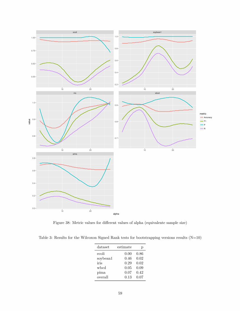
pima
iris wbcd
ecoli soybean1
10 20
10 20 10 20
10 20 10 20
0.2
0.4
0.6
0.8
1.0
0.7
0.8
0.9
0.25
0.50
0.75
1.00
0.8
0.9
1.0
0.0
0.2
0.4
0.6
0.8
alpha
value
metricAccuracy
F1
P
R
Figure 38: Metric values for di�erent values of alpha (equivalente sample size)
Table 3: Results for the Wilcoxon Signed Rank tests for bootstrapping versions results (N=10)
dataset estimate pecoli 0.00 0.86soybean1 0.46 0.02iris 0.29 0.02wbcd 0.05 0.09pima 0.07 0.42overall 0.13 0.07
59

pima
iris wbcd
ecoli soybean1
0.00 0.25 0.50 0.75 1.00
0.00 0.25 0.50 0.75 1.00 0.00 0.25 0.50 0.75 1.00
0.00 0.25 0.50 0.75 1.00 0.00 0.25 0.50 0.75 1.00
0.25
0.50
0.75
1.00
0.6
0.7
0.8
0.9
0.25
0.50
0.75
1.00
0.7
0.8
0.9
1.0
0.25
0.50
0.75
gamma
value
metricAccuracy
F1
P
R
Figure 39: Metric values for di�erent values of gamma (rebalance constant)
60

pima
iris wbcd
ecoli soybean1
2.5 5 7.5 10 12.5 15 17
.5 20 22.5 25
2.5 5 7.5 10 12.5 15 17
.5 20 22.5 25
0
0.1
0.2
0.3
0.4
0.5
0.6
0.7
0.8
0.9
0
0.1
0.2
0.3
0.4
0.5
0.6
0.7
0.8
0.9
0
0.1
0.2
0.3
0.4
0.5
0.6
0.7
0.8
0.9
alpha
gamma
0.00
0.25
0.50
0.75
1.00value
Figure 40: F1 values for di�erent combinations of gamma and alpha
61

P R
Accuracy F1
0.00 0.25 0.50 0.75 1.00 0.00 0.25 0.50 0.75 1.00
ecoli
soybean1
iris
wbcd
pima
ecoli
soybean1
iris
wbcd
pima
value
dataset
classifierplainBootstrap
plainBootstrap_10
weightedBootstrap
weightedBootstrap_10
Figure 41: Comparison between bootstrap mechanisms
62

P R
Accuracy F1
0.00 0.25 0.50 0.75 1.00 0.00 0.25 0.50 0.75 1.00
ecoli
soybean1
iris
wbcd
pima
ecoli
soybean1
iris
wbcd
pima
value
dataset
classifiernaiveBayes
plainBootstrap
plainBootstrap_10
plainFullBayes
randomForests
weightedBootstrap
weightedBootstrap_10
Figure 42: Classifier comparison
• A Näive Bayes classifier, in a version implemented ad-hoc for this project. The inclusion of NäiveBayes will aid in determining to what extent the structural assumptions made by this classifier (theindependence of the features given the class) impact the real classification performance.
• A Random Forests classifier, taken from the implementation in R’s Caret package. Both the algorithmand the implementation are known to have a good general performance, so this value will give us anindication on the expected maximum accuracy for the dataset.
Both classifiers where mainly included to stablish a reference level in the classification di�culty of the datasets.Since the goal of full Bayesian Classifiers is broader than that of other specialized classifiers (as the BC aimsto capture an expression for the joint distribution the underlying distribution that generated the dataset), alower classification accuracy is expected when compared with classification-oriented models.
Figure 42 shows the results for di�erent metrics for all the classifiers tested in the experiments. Color bandswere added as a visual aid for tight boxplots.
Tables 4 and 5 show, respectively, the results of the Wilcoxon Signed Rank test for the one to one comparisonof classifiers. Some remarks are clear from the results:
• First of all, as expected, the Random Forests algorithm clearly outperforms all of the other classifiers in
63

Table 4: Estimates from the Wilcoxon Signed Rank tests for classifier comparison
plainBootstrap weightedBootstrap plainFullBayes naiveBayes randomForestsplainBootstrap 0.00 0.07 0.14 0.14 -0.17weightedBootstrap -0.07 0.00 0.03 0.03 -0.27plainFullBayes -0.14 -0.03 0.00 -0.12 -0.49naiveBayes -0.14 -0.03 0.12 0.00 -0.36randomForests 0.17 0.27 0.49 0.36 0.00
Table 5: P-value from the Wilcoxon Signed Rank tests for classifier comparison
plainBootstrap weightedBootstrap plainFullBayes naiveBayes randomForestsplainBootstrap 0.00 0.17 0.06 0.07 1weightedBootstrap 0.83 0.00 0.19 0.36 1plainFullBayes 0.94 0.81 0.00 0.84 1naiveBayes 0.93 0.65 0.16 0.00 1randomForests 0.00 0.00 0.00 0.00 0
the comparison, with a very high confidence.
• The Plain Bootstrap Bayesian Classifier performs better than the rest of the algorithms, excluding theRandom Forests, but the confidence levels are lower in this case. The addition of more experimentscould enhance the confidence in this superiority.
• The simple Full Bayesian Classifier has the worst performance of the ranking, even outperformed by thesimple Näive Bayes classifier. Looking at Figure 42 we can see that this problem may be caused by theextreme variability in performance it has shown during the tests. As we will analyze in the next section.
6.7 Variability and zero-valued F1 metrics
One of the biggest problems we have encountered during the experiments is the inherently variability in thestructure of the induced classifiers. This variability a�ected the learning process in two distinct ways:
• It makes the performance of the classifier somewhat impredictible compared with other learningalgorithms.
• For hard to learn datasets, it generates some null results, where the classifier have zero recall (and soalso zero F1 measure).
Figure 43 shows the number of null experiments for each of the dataset (taken from the heuristic determinationexperiments). We can see how the easier Iris and WBCD datasets have no null entries, while the harderSoybean1 dataset has more null entries than positive ones. This condition compromises the utility of theclassifier under real data, but this extreme results seem to be due to an error in the structure inductionprocess, that should not be hard to spot.
In order to shed light on the problem, some additional experiments were conducted, using the same settingsas per the heuristic process, in order to measure some characteristics of the null vs. not null solutions.
Figure 44 shows boxplots for the values of the di�erent characteristics for all the datasets.
64

0
5
10
15
20
25
ecoli iris pima soybean1 wbcddataset
count nullValue
null
positive
Figure 43: Number of zero values per dataset
65

totalArcs
H IR MLE
ClassParents frqMean frqMedian
10 100
0.1 1e+04 1e+06
1 10 1 10 100 1 10 100
ecoli
iris
pima
soybean1
wbcd
ecoli
iris
pima
soybean1
wbcd
ecoli
iris
pima
soybean1
wbcd
ecoli
iris
pima
soybean1
wbcd
ecoli
iris
pima
soybean1
wbcd
ecoli
iris
pima
soybean1
wbcd
ecoli
iris
pima
soybean1
wbcd
value
dataset nullValue
null
positive
Figure 44: Characteristics analysis for null cases
66

7 Conclusions
This project aimed to analyze one important problem in the field of Machine Learning Classification: theclass imbalance problem. The problem was described thoroughly, as were the metrics used to diagnose it. Along study of the State of the Art was conducted, showing the most relevant solutions found in the literatureto tackle with the problem. Building on these ideas and on the theory behind Bayesian Classifiers, somealgorithm modifications were proposed to try to improve the performance of the basic algorithms behind theBCs.
Three improvements were proposed and implemented in order to deal with the class imbalance problem: therectification of the Mutual Information term in the structure induction; the rebalance of the parameter priorsbased on the imbalance; and the use of bagging ensembles based on the probability of occurrence of the testexamples. Another proposal was defined in the analysis section (the use of fine-grained prior control), but wasnot implemented due to the lack of time. Experiments were conducted for all the implemented features, andits performance was compared with other well known classifiers, to stablish a reference of the classificationdi�culty.
For the case of the rectification, the results are ambiguous, as it had a positive e�ects in some datasets and anegative e�ects in other. It also made worse the null performance error described in the last section of theexperiments for all datasets. In the case of the parameter priors, some evidence was found that both theequivalent sample size and the rebalance a�ected the performance of the classifiers, depending on the dataset,but due to small size of the experiments, its high variability generated a low confidence in the results. Thelast proposal, the use of a probabilistic-weight Bagging Ensemble, was outperformed by the most simple plainaverage of bootstrapped models (although it succeeded in improving the global performance of the plainBayesian Classifier).
The tight project schedule imposed a reduction in the number of experiment replicas that could be executedas well as in the number of features of the implementation. As Figure 1 in the introduction reflects, alarge part of the project was spent in State of the Art documentation and prototyping, while most of theimplementation and experimentation was delayed until the last months of the project. This restriction forcedto limit the scope of the implementation, and reduced the number of replicas for each experiment and thenumber of datasets originally selected (what led in turn to a reduction in the significance of the results).
A clear future line of development would be to extend the scope of the experiments, both in number of datasetsand in replicas, in order to strengthen the significance of the results (leading to the confident acceptanceor rejection of the proposed implementations). Another assertion that was suggested in the analysis (thetheoretical simmilarity of some of the resampling mechanisms with prior rebalancing) remains untested, andcould shed light on how to more appropriately use those priors to make a skew-insensitive BC.
The implementation of the classifier itself should also be improved. A small percentage of the inducedclassifiers showed abnormal zeroed metrics, a behavior that may be caused by an implementation bug or acharacteristic in the induced model that we hope to be able to statically diagnose from the induced classifier(and so, to solve it in training time). It should also be easy to broaden the classifier scope by acceptingmulticlass problems and missing values (so taking some advantage of the BCs specific capabilities).
As a last line of improvement in the analysis side, it would also be important to perform another set ofexperiments focusing on testing with which degree of accuracy does the implemented classifier induce theappropriate dataset distribution, not only regarding classification, but also regarding the precision with whichthe probability distribution is captured
67

8 Appendix A. Classifier Implementation
In order to execute the designed experiments, and to allow all the desired parameters to be changed, aBayesian Classifier was implemented from scratch, as an R library. To simplify the implementation, theBC was chosen to work only with discrete binary values and complete data (making the implementationmulticlass and able to deal with missing data should be straightforward, due to the nature of the BC).
In order to facilitate the experiments, the implementation was made very configurable, in order to testall the options and metaparameters described in the experiments. Three basic algorithmic variants wereimplemented:
• scoring: score function to use in the training process: “bic” or “mle”.
• discretization: method used for the discretization of numerical data: “equalFreq” or “topDown”. Thefirst discretization method was built into the classifier code: it divides the training data into N bucketsof the same size, taking the top value of each bucket as the breaking point for the discretization. The“topDown” was chosen from the available algorithms in R’s ‘discretization’ package.
• heuristicSearch: metaheuristic algorithm used to search for the optimal structure: ‘rb’ (RandomizedBias), or ‘hc’ (Hill Climbing).
• rectifiedMI: use of the recification of the Mutual Information: true or false.
All this options can be combined together in any way, giving rise to eight possible basic variations of theclassifier. To simplify the experiments, a default value was selected for each options, so only the option beingtested was changed for each experiment. The default values were: “bic”, “equalFreq” and “rb”.
Here is a list of the implemented metaparameters:
• –: equivalent sample size for the Dirichlet prior distributions.
• “: balance level between the values that make up the equivalent sample size. Used in the experimentsto balance the prior distribution against the imbalance rate.
• Ï: this parameter controls the amount of rectification of the Mutual Information in case the rectifiedMIflag were active.
• C: this structure constant multiplies the regularization term in the BIC score function. It can beused to regulate the target complexity of the induced model (the greater the constant, the lower thecomplexity of the model).
Apart from the implementation of the Bayesian Classifier, a Bootstrap Aggragating module was created inorder to create the ensambles to test. All the weak classifiers for the ensemble are instances of the plainBayesian Classifier. Two options of classifier combination were implemented: one with a simple average ofmodels and another one that weighted each classifier based on the normalized probability that it assigned toeach of the test instances.
68

9 Appendix B. Datasets
9.1 Real-world datasets
In order to asess the influence of the imbalance level in the classification error, several reallife datasets willbe used, among those most frequent in the literature. Most of them come from the UCI Machine LearningRepository [38]:
• Pima Indians Diabetes Data Set [39]
• Breast Cancer Wisconsin (Diagnostic) Data Set [40]
• Abalone Data Set [41]: this is not strictly speaking a classification problem, as it consists in guessingthe age of the specimen given the other traits. We follow the approach finding in the literature ofclassifying the specimens as less than 19 years-old (negative class) or equal or greater (positive class).
• Ecoli Data Set [42]: this is a multiclass classificaiton problem. Since in this preliminar experiments weare dealing with binary classification problems, we will consider the problem of deciding whether theprotein is localized in the outer membrane.
• Thyroid Data Set [43]: this dataset is actually broken into other smaller ones. We have selected thefollowing ones: “sick”, “allhypo” and “allrep”
• Yeast Data Set [44]: this is also a multiclass dataset; it will be transformed into a binary classificationproblem by selecting a subset of the classes as positive. Following the approach in [45] just the “POX”and “CYT” classes will be considered as positive classes.
• Iris Data Set [46]: one of the most common datasets in the classification literature, it describes specimensof Iris from three diferent species: Setosa, Versicolor and Virginica.
• Soy Bean Data Set [47]: another classical dataset regarding Soy Bean diseases.
For all the datasets that provided a partition in test and training data, that partition has been honored. Forthose who not, a random partition is created on loading, dividing the dataset in 85% of training data and15% of test data.
Prior to its use in the experiments, all the datasets were cleaned, i.e.: missing values were removed, and typeswere adjusted to avoid format problems in the training step.
All the datasets were collected into an R Package for ease of management.
Due to time restrictions, most of the experiments were restricted to the following list of datasets: ecoli,soybean1, iris, wbcd and pima.
Table 6 shows the summary of the dataset information ordered by Imbalance Rate:
9.2 Synthetic datasets
All examples from the problem description section are generated using synthetic datasets, with the requiredcharacteristics. All the datasets consist of random instances drawn from two distributions, in a space formedby two numeric variables X and Y , and a target binary class that select the distribution. Each distributionis composed of a set of clusters of examples, normally distributed around a center point (with all the centerpoints located in a rectangular grid around the origin).
The following subsections describe how each of the characteristics of the dataset are generated.
69

Table 6: Summary of real-life datasets information
dataset examples features irabalone 4177 9 0.02soybean3 683 36 0.03allrep 3772 28 0.03ecoli 336 8 0.06sick 3772 28 0.06soybean2 683 36 0.06allhypo 3772 28 0.08soybean1 683 36 0.13yeast 1484 10 0.33iris 150 5 0.33wbcd 699 10 0.34pima 768 9 0.35ionosphere 351 34 0.64
9.2.1 Complexity
The complexity level of the dataset is determined by the number of normal distributions that compose eachcluster. The number of generated clusters is 2n with n the complexity number, with all the cluster centerslying in an evenly spaced grid around the origin.
9.2.2 Interclass imbalance
Interclass imbalance is changed by modifying the probability that a new example have of being drawn froma particular disjunct of the minority class. When this factor has the value 1, all the disjuncts have equalprobability, and so, the examples tend to be evenly distributed among disjuncts. Higher values generate moreskewed distributions, using the following expressions:
P̃ (c) = 1.75 ú (d ≠ 1)c
P (ci) = P̃ (ci)qxœC
P̃ (x)
Where C = 1, 2, ...Nc is each of the cluster identifiers.
9.2.3 Overlap between classes
Since all the synthetic datasets are composed of sets of normally distributed clusters, the degree of overlapbetween them will be governed by the standard deviation of those normal distributions. These deviations arecalculated as:
‡ = WG
6 ≠ Lo
Where WG is the width of each square of the grid where the clusters are allocated (a parameter that dependson the complexity level) and Lo the overlap level (that vary from 1 to 5 in the experiments).
70

Bibliography
[1] A. Solanas et al., “Smart health: A context-aware health paradigm within smart cities,” IEEE Communi-cations Magazine, vol. 52, pp. 74–81, IEEE, 2014.
[2] A. Solanas, F. Casino, E. Batista, and R. Rallo, “Trends and challenges in smart healthcare research: Ajourney from data to wisdom,” 2017 IEEE 3rd International Forum on Research and Technologies for Societyand Industry (RTSI), pp. 1–6, IEEE, 2017.
[3] D. Koller and N. Friedman, “Learning,” Probabilistic Graphical Models, pp. 695–1006, MIT Press, 2009.
[4] D. Koller, “Probabilistic graphical models specialization,” 2009. [Online].Available: https://www.coursera.org/specializations/probabilistic-graphical-models .
[5] J. Ortigosa-Hernández, I. Inza, and J. Lozano, “Towards competitive classifiers for unbalanced classificationproblems: A study on the performance scores,” 2016.
[6] C. Sei�ert, T. M. Khoshgoftaar, J. V. Hulse, and A. Napolitano, “RUSBoost: A hybrid approach toalleviating class imbalance,” IEEE Transactions on Systems, Man, and Cybernetics - Part A: Systems andHumans, vol. 40, pp. 185–197, IEEE, 2010.
[7] G. M. Weiss and F. Provost, “Learning when training data are costly: The e�ect of class distribution ontree induction,” Journal of Artificial Intelligence Research 19, pp. 315–354, AAAI Press, 2003.
[8] T. Jo and N. Japkowicz, “Class imbalances versus small disjuncts,” SIGKDD Explorations Newsletter, vol.6, pp. 40–49, ACM, 2004.
[9] N. Japkowicz, “Class imbalance: Are we focusing on the right issue?” Notes from the ICML Workshop onLearning from Imbalanced Data Sets, 2003.
[10] N. Tomaöev and D. MladeniÊ, “Class imbalance and the curse of minority hubs,” Knowledge-BasedSystems, vol. 53, pp. 157–172, Elsevier Science Publishers B. V., 2013.
[11] V. López, A. Fernández, S. García, V. Palade, and F. Herrera, “An insight into classification withimbalanced data: Empirical results and current trends on using data intrinsic characteristics,” InformationSciences, vol. 250, pp. 113–141, Elsevier, 2013.
[12] N. Japkowicz and S. Stephen, “The class imbalance problem: A systematic study,” Intelligent DataAnalysis, vol. 6, pp. 429–449, IOS Press, 2002.
[13] M. Denil and T. Trappenberg, “Overlap versus imbalance,” Advances in Artificial Intelligence, pp.220–231, Springer Berlin Heidelberg, 2010.
[14] M. Wasikowski and X. w. Chen, “Combating the small sample class imbalance problem using featureselection,” IEEE Transactions on Knowledge and Data Engineering, vol. 22, pp. 1388–1400, IEEE, 2010.
[15] M. Khun, “A short introduction to the caret package,” 2016. [Online].Available: https://cran.r-project.org/web/packages/caret/vignettes/caret.html .
[16] N. V. Chawla, K. W. Bowyer, L. O. Hall, and W. P. Kegelmeyer, “SMOTE: Synthetic minority over-sampling technique,” Journal of Artificial Intelligence Research, vol. 16, pp. 321–357, AI Access Foundation,2002.
[17] H. Han, W.-Y. Wang, and B.-H. Mao, “Borderline-smote: A new over-sampling method in imbalanceddata sets learning,” Advances in Intelligent Computing, pp. 878–887, Springer Berlin Heidelberg, 2005.
[18] H. He and E. Garcia, “Learning from imbalanced data,” Knowledge and Data Engineering, IEEETransactions on, vol. 21, pp. 1263–1284, IEEE, 2009.
[19] M. Kubat and S. Matwin, “Addressing the curse of imbalanced training sets: One-sided selection,”In Proceedings of the Fourteenth International Conference on Machine Learning, pp. 179–186, Morgan
71

Kaufmann, 1997.
[20] G. E. A. P. A. Batista, R. C. Prati, and M. C. Monard, “A study of the behavior of several methods forbalancing machine learning training data,” SIGKDD Explorations Newsletter, vol. 6, pp. 20–29, ACM, 2004.
[21] G. Weiss, “Foundations of imbalance learning,” Imbalanced Learning Foundations, Algorithms, andApplications, pp. 13–43, Wiley-IEEE Press, 2013.
[22] M. Galar, A. Fernandez, E. Barrenechea, H. Bustince, and F. Herrera, “A review on ensembles for theclass imbalance problem: Bagging-, boosting-, and hybrid-based approaches,” IEEE Transactions on Systems,Man, and Cybernetics, Part C (Applications and Reviews), vol. 42, pp. 463–484, IEEE, 2012.
[23] Y. Sun, M. S. Kamel, A. K. Wong, and Y. Wang, “Cost-sensitive boosting for classification of imbalanceddata,” Pattern Recognition, vol. 40, pp. 3358–3378, Elsevier, 2007.
[24] X. Y. Liu, J. Wu, and Z. H. Zhou, “Exploratory undersampling for class-imbalance learning,” IEEETransactions on Systems, Man, and Cybernetics, Part B (Cybernetics), vol. 39, pp. 539–550, IEEE, 2009.
[25] Y. Freund and R. E. Schapire, “A decision-theoretic generalization of on-line learning and an applicationto boosting,” Journal of Computer and System Sciences, vol. 55, pp. 119–139, Academic Press, Inc., 1997.
[26] S. Wang and X. Yao, “Diversity analysis on imbalanced data sets by using ensemble models,” 2009 IEEESymposium on Computational Intelligence and Data Mining, pp. 324–331, IEEE, 2009.
[27] K. M. Ting, “An instance-weighting method to induce cost-sensitive trees,” IEEE Transactions onKnowledge and Data Engineering, vol. 14, pp. 659–665, IEEE, 2002.
[28] M. Maloof, “Learning when data sets are imbalanced and when costs are unequal and unknown,” Notesfrom the ICML Workshop on Learning from Imbalanced Data Sets, 2003.
[29] P. Domingos, “MetaCost: A general method for making classifiers cost-sensitive,” Proceedings of theFifth ACM SIGKDD International Conference on Knowledge Discovery and Data Mining, pp. 155–164, ACM,1999.
[30] C. Elkan, “The foundations of cost-sensitive learning,” Proceedings of the 17th International JointConference on Artificial Intelligence - Volume 2, pp. 973–978, Morgan Kaufmann Publishers Inc., 2001.
[31] F. Provost and P. Domingos, “Tree induction for probability-based ranking,” Machine Learning, vol. 52,pp. 199–215, Springer, 2003.
[32] R. Vilalta and D. Oblinger, “A quantification of distance bias between evaluation metrics in classification,”Proceedings of the Seventeenth International Conference on Machine Learning, pp. 1087–1094, MorganKaufmann Publishers Inc., 2000.
[33] P. A. Flach, “The geometry of roc space: Understanding machine learning metrics through roc isometrics,”in Proceedings of the Twentieth International Conference on Machine Learning, pp. 194–201, AAAI Press,2003.
[34] D. A. Cieslak and N. V. Chawla, “Learning decision trees for unbalanced data,” Machine Learning andKnowledge Discovery in Databases, pp. 241–256, Springer Berlin Heidelberg, 2008.
[35] A. A. Juana, I. Pascuala, D. Guimaransb, and B. Barriosa, “Combining biased randomization withiterated local search for solving the multidepot vehicle routing problem,” International Transactions inOperational Research, pp. 647–667, Wiley, 2014.
[36] M. J. Flores and J. A. Gamez, “Impact on bayesian networks classifiers when learning from imbalanceddatasets,” International Conference on Agents and Artificial Intelligence, vol. 2, pp. 382–389, SciTePress,
72

2015.
[37] D. Heckerman, “A tutorial on learning with bayesian networks,” Innovations in Bayesian Networks:Theory and Applications, pp. 33–82, Springer Berlin Heidelberg, 2008.
[38] “UCI machine learning repository.” [Online].Available: https://archive.ics.uci.edu/ml/index.php .
[39] V. Sigillito, “Pima indians diabetes data set,” 1990. [Online].Available: https://archive.ics.uci.edu/ml/datasets/pima+indians+diabetes .
[40] Wolberg, Street, and Mangasarian, “Breast cancer wisconsin (diagnostic) data set,” 1995. [Online].Available: https://archive.ics.uci.edu/ml/datasets/Breast+Cancer+Wisconsin+(Diagnostic) .
[41] Nash, Sellers, and Talbot, “Abalone data set,” 1994. [Online].Available: https://archive.ics.uci.edu/ml/datasets/abalone .
[42] K. Nakai, “Ecoli data set,” 1996. [Online].Available: https://archive.ics.uci.edu/ml/datasets/ecoli .
[43] R. Quinlan, “Thyroid disease data set,” 1986. [Online].Available: http://archive.ics.uci.edu/ml/datasets/thyroid+disease .
[44] K. Nakai, “Yeast data set,” 1996. [Online].Available: https://archive.ics.uci.edu/ml/datasets/Yeast .
[45] L. Nanni, C. Fantozzi, and N. Lazzarini, “Coupling di�erent methods for overcoming the class imbalanceproblem,” Neurocomputing, vol. 158, pp. 48–61, Elsevier, 2015.
[46] R. Fisher, “Iris data set,” 1936. [Online].Available: https://archive.ics.uci.edu/ml/datasets/iris .
[47] Michalski and Chilausky, “Soybean data set,” 1980. [Online].Available: https://archive.ics.uci.edu/ml/datasets/Soybean+(Large) .
73