market connectedness: return vs. volatility...
TRANSCRIPT

Market Connectedness:
Return vs. Volatility Spillovers∗
NAROD ERKOL†
June 8, 2015
1 Introduction
Economic entities are becoming more and more interconnected with each other and the
overall degree of international equity market connectedness has been increasing espe-
cially over the past two decades. Although, there is an evidence that there is a strong
connection among markets, new approaches of measuring and quantifying the connection
and understanding its dynamics are still being developed.
We measure the connectedness using the stock market data because of the advantages
to analyze the economic links between two countries on the basis of stock market data,
rather than aggregate economic data published by national statistical offices, is that
stock market data are readily available, allowing analysis in almost real time.
To measuring the connectedness, I have three different purposes in my PhD thesis.
First, we measure the connectedness of different stock markets using return spillovers
by the methodology of Diebold and Yilmaz [2]. My contribution in this case, will be
not only looking on the return spillovers but also develop a methodology to measure the
connectedness by using volatility-to-volatility spillovers. The details of the method will
be explained in the following sections of this paper. But for now, we need to emphasize
that to compute the volatility spillovers we need the weekly volatility series of each
market. To do this, we develop a methodology to obtain the weekly volatility series
using the German and Klass [14] methodology. Below, we will explain the objective of
this methodology and the intuition behind it.
One of the approach to measure equity market connectedness, which we mentioned
above, is based on forecast error variance decomposition, developed by Diebold and
Yilmaz [2], and extensions of this approach to assess the propagation of information
across markets, developed by Schmidbauer, Rosch and Uluceviz [8].
∗I would like to thank my supervisor Javier Asensio and Harald Schmidbauer for their support and
suggestions during the development of this paper.†Universitat Autonoma de Barcelona, Barcelona, Spain; e-mail: [email protected]
1

One way to quantify market connectedness is to estimate the variance of the error
when forecasting future return or return volatilities on the asset price. Diebold and
Yilmaz [2] [3] use this idea to develop a network view of markets as nodes and weights
determined by variance shares. They decompose the error variances of joint asset return
forecasts, using the vector autoregressive (VAR) models. In terms of their approach, the
decomposed error variances present a network with assets as nodes and the weights of
links between nodes determined by shares of forecast error variance spillovers. Using
this methodology, pairwise spillovers can be discussed, but their goal is to go one step
further and designate the degree of market connectedness. They suggest a measure for
the degree of market connectedness which they call the spillover index.
Schmidbauer, Rosch and Uluceviz [8] extend the spillover index methodology and
quantify dynamically the amount of connectedness of markets with a focus on the flow
of information. They use the concepts of Kullback-Leibler divergence developed by
Demetrius [1] and Tuljapurkar [13] to measure the amount of market connectedness dy-
namically. Schmidbauer, Rosch and Uluceviz [8] discuss the Kullback-Leibler divergence
in the field of market connectedness and define the relative market entropy approach.
First market entropy, measures the amount of information created every period, and the
second one quantifies the speed of information digestion in the system. Building on the
framework developed by Diebold and Yilmaz [2], they construct supplementary measures
of market connectedness using information theory and population dynamics.
The first purpose of the present paper is to use these two methodologies developed
by Diebold and Yilmaz [2] and Schmidbauer, Rosch and Uluceviz [8] with weekly return
and weekly return volatility series and to interpret the different and similar outcomes of
market connectedness in the case of using the expectation and the standard deviation of
assets. The main goal is to analyze the market with respect to different structures, in our
case, using the expectation of the prices and plus using the variations of them as a data.
Using the spillover and entropy approach, we want to compare the results of market
connectedness while return series is used and on the other hand, return volatility series
is used instead of return. Analysing not only the return series but also the variations
of them will give us an information about how do they complement each other. So, the
main goal is to quantify dynamically the amount of connectedness of markets with a
focus on the spillover and the flow of information and apply the methodologies using
weekly return and weekly return volatility data. Therefore, this will give a chance to
analyze different interpretations of market connectedness that comes from either using
the expectation of the prices or using the variations of them. As it will be explained in
Section 3.1.1, to compute the volatility spillovers we need to obtain the weekly volatility
series. We developed a methodology using the Brownian motions idea. We simulate
brownian motions to have an intuition for the estimation of volatility series. There
are still limitations of our study, so the next attempt will be to solve the problems of
this method and use this new method to obtain the volatility series and compute the
volatility-to-volatility spillovers. Rather then the German and Klass approach we have
also calculated the volatility spillover using daily volatility estimated by the GARCH
2

methodology. One of the purpose of this study is to compare the methodologies of
volatility estimation and find the suitable one for our study. In the Empirical part, we
compared the German and Klass and GARCH approach and analyse them in terms of
volatility spillovers.
Second purpose of the present study, will be the investigation about the connected-
ness of Turkish stock market using an extended methodology of spillover index. We try
to answer the question that which countries or organisations is Turkish stock market
affected from. To do this, for now, we only analyse the return-to-volatility spillovers
using the weekly return series of the stock market. We analyse the connectedness from
four groups of countries to the Turkish stock market. For this purpose, we grouped the
stock markets and not using them as a separate stock markets as before, we improved
a new methodology, based on the principal component analysis, to omit the exagger-
ated influence of the large groups, since the groups are unequally large. We leave the
theoretical explanation of this method as a future study of the thesis.
Interpreting the return spillovers will give us a chance to see the connectedness from
the other groups of stock markets to Turkish stock market and the differences of this
connectedness in the past decade. In the present paper, we will explain the results of the
return spillovers and comment on them. We will also examine the from Turkey to Turkey
connectedness to see the effect of itself. From the Section 5.2 we can conclude that the
relation from Turkey to Turkey is increased in the last five years. In my future study, I
will try to examine the reasons of this increase and find a specific economic or political
events which causes this increase in the internal connectedness. The interpretation of the
increase in the connectedness of Turkey and the Islamic countries will be also explained
in the future studies. Then, we will also improve the methodology that we use for the
case of Turkey and apply it using also the volatilities and not only the returns.
Third, as we explain the entropy methodology in Section 2.2 we will also use the
KLIC and KS entropy idea in the case of Turkey and try to compare the method that we
developed. Since, by using the entropy idea we have a feeling about the information that
is produced by the system in every week and also the digestion period of this information
from the system, we can utilise the entropy idea to interpret the reasons of the changes
in the connectedness of the stock markets in the last 15 years.
The data that we used in this study divided into three parts to measure the connect-
edness with respect to two different goals. The first method used in the present paper
is illustrated using data from the stock markets of five countries : Dow Jones Industrial
Average (USA, New York Stock Exchange), FTSE (UK, London Stock Exchange), DAX
(Germany, Frankfurt Stock Exchange), CAC40 (France, Euronext Paris), Nikkei 225
(Japan, Tokyo Stock Exchange). The weekly return and weekly return volatility data
are used to apply spillover and entropy methodologies. R-project is used to apply the
methodologies for both return and return volatility data.
The second one, uses daily closing quotations of the Russian stock index and the
five stock indices representing stock markets in the ”Systemic Five” countries. We will
compute return spillovers using the same methodology with the first data set, but for
3

the volatility spillovers we will use the GARCH methodology instead of the German and
Klass.
The third one, the case of Turkey, uses 36 different stock markets of different countries
where we grouped them into four parts with respect to their region or the organisations
that they involve. The groups are: European union countries (EU), Organisation of the
Islamic Conference countries (OIC), Brazil, Russia, India and China as in the group of
BRIC, USA and Turkey itself.
This paper is organized as follows. Section 2, describes the methodologies of re-
turn spillovers and entropy. It is a review of the spillover methodology developed by
Diebold and Yilmaz [2] and entropy methodology developed by Schmidbauer, Rosch and
Uluceviz [8]. Section 3 is the methodology of volatility spillovers which we develop and
KLIC and KS entropy using volatility series. The method of obtaining volatility is ex-
plained using the idea developed by German and Klass [14]. The intuition of estimating
the volatility series is explained in detail in this section. We have also explained the
GARCH methodology of estimating the volatility series. Section 4 describes some prop-
erties of the three groups of data and explains how to obtain the weekly/daily return and
weekly/daily volatility series for the first group. Empirical results of the two method-
ologies, explained in Section 2 and 3, are presented in Section 5.1 for both spillovers and
entropy and with two estimation methodology of volatility spillovers and the compari-
son of them. The results of market connectedness for the case of Turkey using return
spillovers is explained in Section 5.2. Section 6 concludes and discusses suggestions for
further research.
2 Methodology I: Measuring return spillovers and
shock repercussions
2.1 Return spillovers using forecast error variance decomposi-
tion (fevd)
Given a multivariate N return series, the forecast error variance decomposition obtained
from fitting vector autoregressive (VAR) models to windows of return data. This method-
ology can be briefly summarized as follows:
1. Fit a standard VAR (vector autoregressive) model to the series.
2. Establish an n period ahead forecast.
3. Decompose the error variance of the forecast for each component with respect to
shocks from the same or other components at time t.
4. Following Diebold and Yilmaz [2], for each market, arrange the fevd.
4
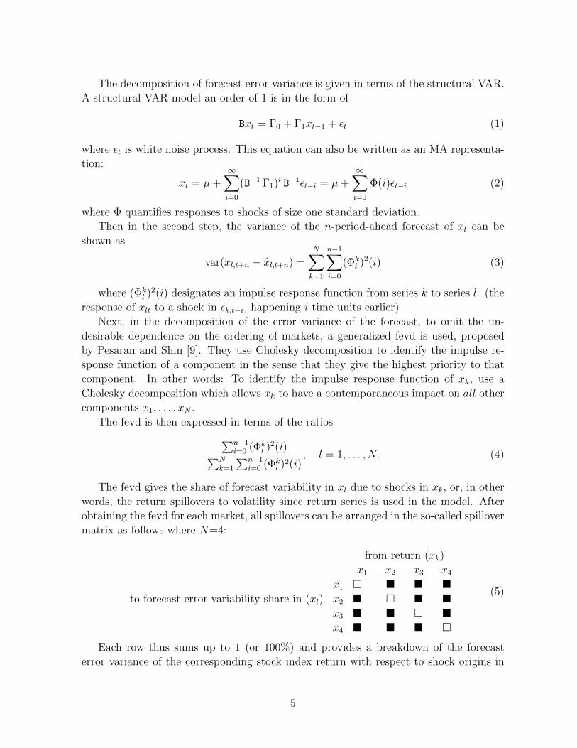
The decomposition of forecast error variance is given in terms of the structural VAR.
A structural VAR model an order of 1 is in the form of
Bxt = Γ0 + Γ1xt−1 + εt (1)
where εt is white noise process. This equation can also be written as an MA representa-
tion:
xt = µ+∞∑i=0
(B−1 Γ1)i B−1εt−i = µ+
∞∑i=0
Φ(i)εt−i (2)
where Φ quantifies responses to shocks of size one standard deviation.
Then in the second step, the variance of the n-period-ahead forecast of xl can be
shown as
var(xl,t+n − xl,t+n) =N∑k=1
n−1∑i=0
(Φkl )
2(i) (3)
where (Φkl )
2(i) designates an impulse response function from series k to series l. (the
response of xlt to a shock in εk,t−i, happening i time units earlier)
Next, in the decomposition of the error variance of the forecast, to omit the un-
desirable dependence on the ordering of markets, a generalized fevd is used, proposed
by Pesaran and Shin [9]. They use Cholesky decomposition to identify the impulse re-
sponse function of a component in the sense that they give the highest priority to that
component. In other words: To identify the impulse response function of xk, use a
Cholesky decomposition which allows xk to have a contemporaneous impact on all other
components x1, . . . , xN .
The fevd is then expressed in terms of the ratios∑n−1i=0 (Φk
l )2(i)∑N
k=1
∑n−1i=0 (Φk
l )2(i)
, l = 1, . . . , N. (4)
The fevd gives the share of forecast variability in xl due to shocks in xk, or, in other
words, the return spillovers to volatility since return series is used in the model. After
obtaining the fevd for each market, all spillovers can be arranged in the so-called spillover
matrix as follows where N=4:
from return (xk)
x1 x2 x3 x4x1 � � � �
to forecast error variability share in (xl) x2 � � � �x3 � � � �x4 � � � �
(5)
Each row thus sums up to 1 (or 100%) and provides a breakdown of the forecast
error variance of the corresponding stock index return with respect to shock origins in
5

terms of percentages. Each entry in the spillover table is called a directional spillover.
Schematically, Diebold and Yilmaz [2] introduced the spillover index,∑�∑
� +∑
�. (6)
The network structure of the spillover matrix with respect to the propagation of
shocks is a broad perspective, using the concepts from population, Markov Chain theory
and information theory. The methodology developed by Diebold and Yilmaz [2] is used
in the paper of Schmidbauer, Rosch and Uluceviz [8] where their goal is to extent the
spillover idea and to find supplementary measures of market connectedness. More in-
formation about the spillover methodology can be found in Diebold and Yilmaz [2] and
Schmidbauer, Rosch and Uluceviz [8].
2.2 Shock repercussions and Entropy
The starting point for shock repercussions is the spillover matrix on a given period. As
it is described in the previous section row entries characterize the markets’ exposition
to shocks while the propagation of the shock needs to be read column-wise. Due to the
network structure of the spillover matrix, the population and Markov chain theory is
used by Schmidbauer, Rosch and Uluceviz [8] to answer the following question: How are
future volatilities across markets affected by a hypothetical shock hitting xk on day t?
How can we measure the strength of market repercussions of a shock?
Let Mt denote the spillover matrix for day t. The propagation of the shock across
the markets within day t can take place in a short time interval of unspecified length.
The shock propagation (repercussion of the shock) can be modeled as
ns+1 = Mt · ns, s = 0, 1, 2, . . . , (7)
where a hypothetical shock “news”) of unit size to market i on day t can be denoted
as n0 = (0, . . . , 0, 1, 0, . . . , 0)′. The index s denotes a hypothetical step in information
flow, ns characterizing what remains of the initial shock n0 across markets after s steps.
To investigate the steady-state properties they discussed the eigenvalue structure of the
matrix Mt. The left eigenvector vt, satisfying
v′t = v′t ·Mt (8)
called the“propagation values” of markets. The propagation value can be interpreted as
the relative value of a shock to market k as seed for future variability in the markets. In
other words it quantifies the strength of repercussions in the system of markets when a
hypothetical shock originates from one of the markets.
The next discussion is about the location of the shock which can be explained using
the transition matrices. The propagation values that is explained above can also be
interpreted as stationary distribution of a Markov chain defined on the basis of a spillover
6

matrix. As given, a spillover matrix is not a suitable transformation matrix, because
its rows sum up to 1 but its columns don’t. So, it can be changed by applying the
transformation
Pt = V−1t ·M′t ·Vt, (9)
where the diagonal matrix Vt contains the left eigenvector vt (corresponding to eigenvalue
1) of Mt, and after re-scaling:
π′s =n′s ·Vt
n′0 · vt,
then the Markov chain equation emerges:
π′s+1 = π′s ·PF , s = 0, 1, 2, . . . , (10)
The details about the transformation can be found in Tuljapurkar [13].
The equation can be interpreted as follows: On day t, the initial location of a shock
in the system is given by π0 (a unit vector). The shock moves through the system
according to the Equation (10). The stationary distribution of shock location is given by
the vector of propagation values, which represents the “information equation” or “news
balance” among markets on that day. Detailed information about the transformation
and relation of them with the market connectedness, can be found in Schmidbauer, Rosch
and Uluceviz [8].
The next questions can be as follows: How much information is produced by the
system of markets from day to day? In other words how much information is gained from
today’s to tomorrow’s (or next week’s in the case of using weekly data) news balance
among markets? The question can be answered by applying the concept of Kullback-
Leibler divergence (Kullback-Leibler information criterion, KLIC), which measures the
entropy of day t with respect to day t−1, of the propagation values belonging to day t and
day t+ 1. So, the KLIC measures the relative variability of one probability distribution
πa with respect to the variability of a second distribution πb:
KLIC =∑i
πa(i) · log2
(πa(i)
πb(i)
); (11)
In the concept of market connectedness, KLIC measures the initial information con-
tent of a shock (news) with respect to the news balance between markets in the long
run. This idea is developed by Schmidbauer, Rosch and Uluceviz [8]. In cases where πbcharacterizes the system of markets, KLIC is called the “relative market entropy”.
As it is explained at the beginning of this section, a hypothetical shock to a market
will change the equilibrium, but then the market will “digest” the shock and reach the
equilibrium again. How fast can the market converge back to the equilibrium after being
hit by a shock? An appropriate measure for the speed of convergence is the Kolmogorov-
Sinai (KS) entropy. Demetrius [1] introduced this entropy measure to population theory
7
as“population entropy”; Tuljapurkar [13] relates it to the rate of convergence of a pop-
ulation. The rate of convergence to equilibrium defined as
KS = −∑i,j
π(i) · log2
(ppijij
). (12)
where pij denotes the entries in the transition matrix of the Markov chain as in the
Equation (10) and π(i) are the stationary probabilities. Schmidbauer, Rosch and Uluce-
viz [8] examine the concept developed by Tuljapurkar [13] and adjust the definition in
terms of market connectedness. More information about the methodology can be found
in Schmidbauer, Rosch and Uluceviz [8].
3 Methodology II: Measuring volatility spillovers and
shock repercussions
3.1 Volatility spillovers
Spillovers are important to understand the financial market interdependence. The spillover
intensity is time-varying and this time-variation is fairly different for returns vs. volatil-
ities.
The same fevd methodology is used, as it is in the Section 2, to obtain the volatility
spillovers. The xt in the Equation (2) that we meant return is now means volatility. So,
we forecast the volatilities instead of returns. As in the return spillovers, where we need
weekly return series, in this case we need weekly return volatility series to apply the
VAR methodology for producing volatility spillovers. The methodology to obtain the
return volatility series using the German and Klass’ formula and the intuition behind it
is explained in Section 3.1.1 and the method of applying the formula to our data will be
explained in Section 4.
3.1.1 Obtaining Daily Return Volatilities
There are different estimation methods to obtain the stock return volatility. We followed
the estimation method of German and Klass [14] and try to understand the intuition
behind it. We try to answer the question that why we can use the estimation method of
German and Klass [14] instead of a GARCH methodology or can we modify the formula
in a different way to estimate the volatility series. As, we can see from the Equation 15,
the major difference of the two methodologies are, the German and Klass methodology
uses only today’s information while GARCH uses also the previous information of the
stock prices. The methodology of German and Klass [14] uses the historical opening,
closing, high and low prices to estimate the volatility series. The model assumes that
security prices are governed by a diffusion process of the form,
P (t) = φ(B(t)) (13)
8

where P is the price, t is time and φ is a monotonic time independent transformation
where we can obtain the maximum and minimum values of B and P . B(t) is a diffusion
process with the differential representation
dB = σdz (14)
where dz is a standard Gauss-Wiener process and σ is an unknown constant to be
estimated.
The methodology of German and Klass covers the usual hypothesis of the geometric
Brownian motion of stock prices to estimate the return volatilities of the series. Although,
the starting point of the estimation method is the Brownian motion, they mention some
limitations of this methodology. They did modifications on the estimation method and
use three different estimation methodology. The first one, uses only the opening and
closing prices and the other two uses high and low prices in addition to the opening and
closing prices. Using also high and low prices in the estimation model gives us more
information about the data, since high and low prices during the trading interval gives
us a continuous information about the prices changes while opening and closing prices
are only ‘snapshots’ of the process. Finally, they found the formula below, which have
the best efficiency factor among the three methodologies.
σ2t = 0.511(Ht − Lt)2 − 0.019[(Ct −Ot)(Ht + Lt − 2Ot)− 2(Ht −Ot)(Lt −Ot)]
− 0.383(Ct −Ot)2,
(15)
where Ot (Ht, Ct, Lt) is the natural logarithm of the opening price in day i (daily high,
Friday closing, daily low) in day t. The methodology of how we implement this formula
to obtain the weekly prices, not the daily ones, is explained in Section 4. For simplicity,
we call the stock return volatility series as “volatility series” throughout the paper.
Explaining the coefficients of the Formula 15 is beyond the scope of this project for
now. Instead of asking; “where does the coefficients come from?”, we want to show the
intuition behind the formula. We develop some intuition to understand the methodology.
We use the same approach like in the German and Klass methodology and simulate a
Brownian bridge to understand the intuition behind this estimation method. Brownian
Bridge is formulated as follows;
Xt = Btµ,σ − tB1
µ,σ (16)
where Bt is a Brownian motion with µ and dispersion σ, and 0 ≤ t ≤ 1.
Obviously, X0 and X1 are 0. So, we know the starting and ending points. In contrast
to the Brownian motion we know the ending point of the process which is the closing
price in our case. The idea behind simulating Brownian Bridges is that, if we can find
a relation between the sigma and the maximum and minimum values of the trading
day then we can estimate the sigma, since we have the information about the high and
low stock prices during the trading day. So, we try to answer the question; Can we
9

Figure 1: Simulations
find a relation among the maximum and minimum values and the σ value? In other
words, is it possible to estimate the σ, using the maximum and minimum value of
the stock price. First, we simulate Brownian Bridge where Bts are normally randomized
numbers. We simulate Brownian Bridges using different normally randomized Bts. Then,
we simulate the Brownian Bridge simulations for different σ values. We have Brownian
Bridge simulations with different normalized random Brownian motions. So, now we can
obtain the maximum and minimum values of the Brownian Bridges for every simulation.
Then, we plot the difference of ‘maximum-minimum’ values for different sigmas to see
that whether there is a relation among them. If we can find a relation, it means, we
can estimate a sigma value by using the difference of ‘maximum-minimum’ values of
a Brownian bridge. The graph of ‘maximum-minimum’ for different values of sigma is
expressed in Figure 1.
As we can see from the Figure 1, there is a linear relationship between the ‘maximum-
minimum’ value and the sigma. So, if we know the maximum and minimum value of the
Brownian Bridge (which in our case it will be the high and low prices of stock in day
i) then using this information we can estimate the sigma value. Since, only the slope
differ in the relation of ‘maximum-minimum’ values and sigma, then we can specify an
“average” slope to decide the relation and we can use this average slope to estimate the
sigma value. The histogram of the slope values is given in Figure 2.
10

Figure 2: Histogram of Slopes
As, we can see from the histogram the average of the slopes lies in the interval of
(6,7). Obviously, this is not the value we can see in the Formula 15, but, at least it gives
us an intuition of the methodology. We want to develop our study in the later versions
of the thesis since now the intuition is missing at some parts. We have not answered
some questions, for example, what if we have a drift together with the diffusion. In our
study we always have a zero mean with different sigma values. So, the results will affect
if we have a drift term with the volatility. Second, we want to find a way to estimate
the sigma when the day is not finished due to an holiday or another reason. Now, to
say something about the sigma our assumptions are made such that the day is complete
and will finish at time 1. So, we will try to answer the questions above and improve our
study to understand the methodology in detail.
3.1.2 Garch Methodology
We will compare the different methodologies of estimating volatility series and try to
find the better estimation methodology for our study. For the first step, we will com-
pare the German and Klass [14] methodology explained in Section 3.1.1 and the Garch
methodology As we mentioned in the previous Section, the Garch methodology uses to-
day’s information as well as the previous day’s information of the stock prices. Since the
methodology also effected by the previous days methodology, as we expected we found
that the volatilities are generally higher than what we have found in the German and
11

Klass methodology. Dow Jones (USA) and Gdaxi (Germany) volatilities computed with
German and Klass, and Garch methodology are in Figure 3. To examine which estima-
tion methodology is better for the sake of our project we will analysis the methodology
with the data in the Empirical part 5 and try to compare the results with respect to the
volatility findings.
3.2 Shock repercussions and entropy for volatility
The market entropy is a tool to measure the amount of information, created from week
to week. Comparing the return KLIC and volatility KLIC is very important to analyze
especially the intervals where the behavior of the two are different. We will see in the
Empirical part (Section 5) in detailed that there are different spikes in different times
for return and volatility market entropies.
For the KS entropy, which is the speed of convergence back to the equilibrium after
a shock, it is shown that return and volatility entropies have different characteristics for
some intervals. Especially in the case of some specific events, the speed of information
digestion varies in the case of return and volatility KS entropies. On the other hand,
the KS entropy has another important characteristic. As it is discussed in Section 5 the
overall pattern of KS entropy and spillovers are similar for both return and volatilities.
The same Markov chain approach is used, as in the Section 2.2, to produce the KLIC
and KS entropy. The same methodology is used, which is developed by Schmidbauer,
Rosch and Uluceviz [8], using the weekly volatilitiy series obtained from Equation (15)
instead of weekly return series.
4 Data
4.1 Data for Return vs. Volatility Spillovers -
German and Klass approach
The two methodologies, spillovers and entropy, are used to see how markets are con-
nected. For both return and volatility spillovers and also for return and volatility en-
tropies, 15-year weekly stock market data of five countries are used. They are obtained
from daily local-currency stock market indexes from 1997-01-06 to 2013-07-08 taken from
Yahoo Finance1 and Datastream. The stock market indexes of five countries that are
used, namely: Dow Jones Industrial Average (USA, New York Stock Exchange; in the fol-
lowing called dji), FTSE (UK, London Stock Exchange; ftse), Nikkei 225 (Japan, Tokyo
Stock Exchange; n225), DAX (Germany, Frankfurt Stock Exchange; gdaxi), CAC40
(France, Euronext Paris; fchi). The level series are shown in Figure 4.
To obtain the weekly returns, we calculate the change in log price of close data,
Friday-to-Friday. If the price data for Friday are not available due to a holiday, we use
1http://finance.yahoo.com/
12

0 200 400 600 800
0.00
0.02
0.04
0.06
0.08
Index
ftse
0 200 400 600 800
0.00
0.02
0.04
0.06
Index
gdax
i
Figure 3: Comparison of Garch and German and Klass volatilities
13

Figure 4: The level series
Thursday. In the case where Thursday is still not available we use Wednesday. We
proceed using this method until we reach an available data in the week. Figure 5 gives
an impression of the dynamics of weekly return series as a percentage.
The formula, developed by Diebold and Yilmaz [2], that is explained in the Section 3
is used to estimate the weekly volatilities. Following Garman and Klass (1980) [14] and
Alizadeh (2002) [15], the underlying daily high/low/open/close data is used to obtain
weekly high, low, opening and closing prices to use the values in formula (15). For the
weekly closing price the same method is used as in return: If available, Friday is used as
weekly closing price, otherwise the previous available day is used. If available Monday
is used as a weekly opening price, otherwise the next available day of the week is used.
The highest value from Monday to Friday is used as weekly high price and the lowest
value from Monday to Friday is used as weekly low price. Figure 6 gives an impression
of the development of weekly volatilities.
4.2 Data for Return vs. Volatility Spillovers -
using GARCH approach
The second empirical part consists of daily closing quotations of the Russian stock in-
dex(rts) and the five stock indices representing stock markets in the ”Systemic Five”
countries which we have used most of them in the Session 4.1: Dow Jones Industrial Av-
14

−20
020 dji
−20
020 ftse
−20
020 gdaxi
−20
020 n225
1997 1999 2001 2003 2005 2007 2009 2011 2013
−20
020 fchi
Figure 5: The series of weekly returns
15

00.
025
dji
00.
02
ftse
00.
02
gdaxi
00.
02
n225
1997 1999 2001 2003 2005 2007 2009 2011 2013
00.
02
fchi
Figure 6: The series of weekly volatilities
16
01
23
45
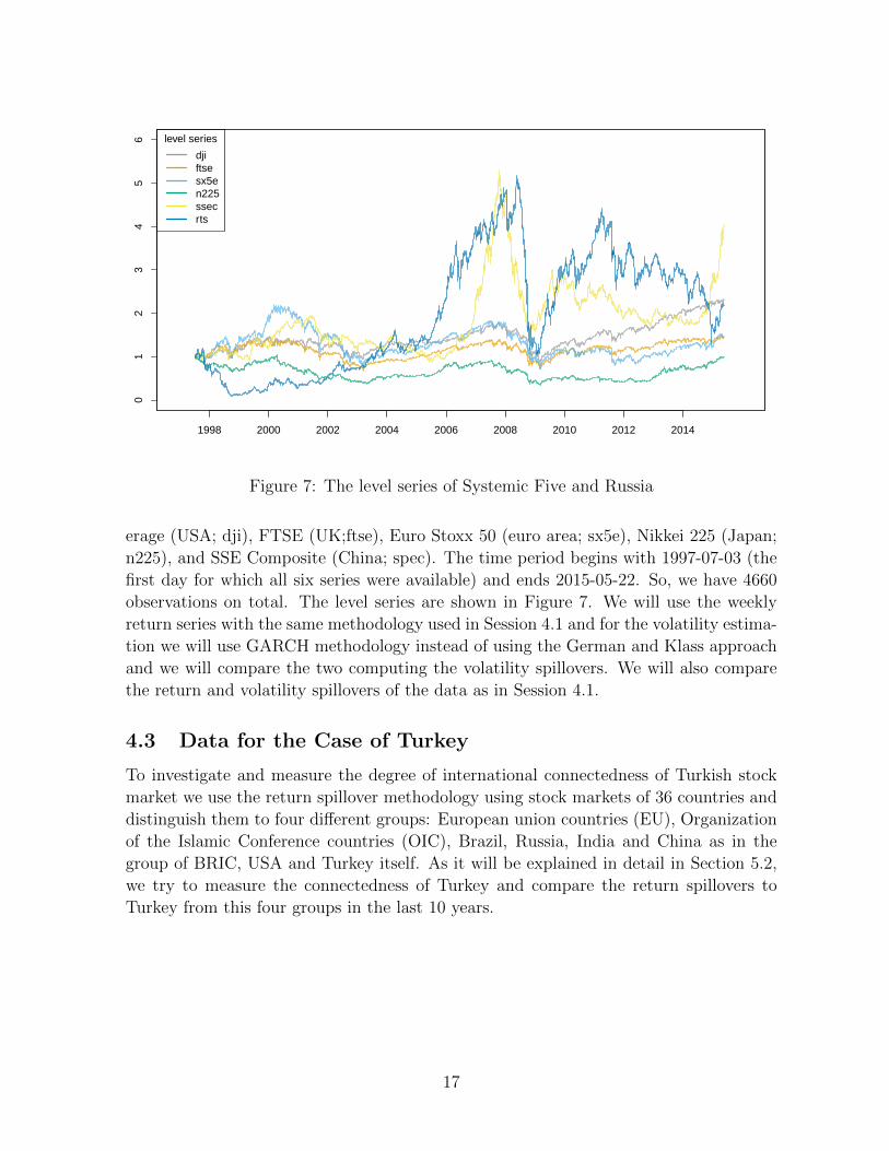
6 level series
djiftsesx5en225ssecrts
1998 2000 2002 2004 2006 2008 2010 2012 2014
Figure 7: The level series of Systemic Five and Russia
erage (USA; dji), FTSE (UK;ftse), Euro Stoxx 50 (euro area; sx5e), Nikkei 225 (Japan;
n225), and SSE Composite (China; spec). The time period begins with 1997-07-03 (the
first day for which all six series were available) and ends 2015-05-22. So, we have 4660
observations on total. The level series are shown in Figure 7. We will use the weekly
return series with the same methodology used in Session 4.1 and for the volatility estima-
tion we will use GARCH methodology instead of using the German and Klass approach
and we will compare the two computing the volatility spillovers. We will also compare
the return and volatility spillovers of the data as in Session 4.1.
4.3 Data for the Case of Turkey
To investigate and measure the degree of international connectedness of Turkish stock
market we use the return spillover methodology using stock markets of 36 countries and
distinguish them to four different groups: European union countries (EU), Organization
of the Islamic Conference countries (OIC), Brazil, Russia, India and China as in the
group of BRIC, USA and Turkey itself. As it will be explained in detail in Section 5.2,
we try to measure the connectedness of Turkey and compare the return spillovers to
Turkey from this four groups in the last 10 years.
17

5 Empirical findings
5.1 Part I: Return Spillovers vs. Volatility Spillovers and En-
tropy
With the stock market data explained in Section 4.1 Section 4.2, market connectedness
can now be obtained by applying methodologies I and II (Section 2 and Section 3) using
weekly returns and weekly volatilities with the German and Klass methodology and daily
return and daily volatility with the GARCH methodology.
5.1.1 Directional and overall spillovers -
Example 1: German and Klass methodology
In this section, we provide an analysis of five countries’ stock market weekly sequences
of return and volatility spillovers (which means, weekly time series of spillover index
values). First, we obtain the spillover matrices which resulted from fitting a sequence of
VAR models along the steps outlined in Section 2 for return spillovers and Section 3 for
volatility spillovers. Moving windows of 100 weeks and 5-week-ahead forecast are used in
the construction of spillover matrices for both return and volatility. The spillover matrix
which is shown in matrix (5) expresses the fraction of the forecast error variance of one
country due to shocks to another country. The ijth entry of the spillover matrix means
estimated contribution to the forecast error variance of country i coming from shocks to
country j.
Each entry in the spillover matrix is called a directional spillover. As an example
of the directional volatility spillover, the US case is shown in Figure 8. As we can see
the early 2000s the spillover that comes from US to the other markets is less than the
spillovers going to US from others. But starting from 2004 until nowadays, on general,
the spillovers that comes from US to the other markets are higher than the spillovers
that come to US from others. It can be said that US is a net sender since mid-2004 in
the sense that during the whole period spillovers coming from US are higher than those
going to US.
Using the moving window of 100 weeks for fitting a sequence of VARs results in a
spillover table for every week. Then using Equation (6) we assess the extent of spillover
variation over time via the corresponding time series of spillover indexes. In other words
the spillover table is an ’input-output’ decomposition of the spillover index.
Overall return and volatility spillovers are displayed in Figure 9 and Figure 10, re-
spectively, together with a smoothed version. Figure 9 is the return spillover from 1997 to
2013. The lowest spillover index is in October 2000 and it started to increase steadily to
about 75% in October 2008 which is the peak date in the whole interval. After October
2008 it was in a decreasing trend and it currently stands at about 67%.
The volatility spillover graph can be seen in Figure 10. The lowest value in this case
is in March 2006 but also in August 2000 the spillover is around 60% which is as low as
18

Figure 8: Directional volatility spillover from/to dji
the minimum value of the spillover series. It started to increase after late 2006 until mid
2010 but unlike the return spillovers it decreased sharply. It currently stands at about
63%.
The comparison between return and volatility spillovers can be more precisely seen in
Figure 11. Generally, volatility spillovers are higher than return spillovers until the end
of 2006 and they only overlap in the period around mid 2006 which is also the time that
volatility is at its lowest value. There are two time intervals that are attracting attention
immediately by looking at the figure. From late 2008 to September 2010, both spillovers
are in their peak values and move together. Similarly, starting from the beginning of 2011
both but especially volatility spillovers decreased sharply until nowadays. Specific events
in these two time intervals have parallel impacts on return and volatility spillovers. On
the other hand, there are other time intervals where one affected more then the other.
Since, if the effect of a shock stays short it can be seen more in the volatility spillovers
rather than in the return and in such a case it is hard to realize the effect of the shock
in the return spillovers. In Figure 12 return spillovers are indicated in the x-axis and
volatility spillovers in the y-axis.
In Figure 12, the comparison of return and volatility spillovers are shown. As it can
be seen directly from the graph the values are positively correlated and the volatility
spillovers are around 10% higher than return spillovers. There are also outlier values
where specific events can explain the reason of this values. For example, the date of
19

terrorist attacks in U.S., September 11, 2001 is an outlier in the graph. The terrorist
attacks launched by the Islamic terrorist group al-Qaeda, in the United States in New
York City and the Washington, D.C. metropolitan area on Tuesday, September 11, 2001.
The subsequent week September 17, 2001 the jump in volatility spillovers can be seen in
the figure as an outlier. On 2001-09-17, the volatility spillover was 72.4% whereas the
return spillover was 53.9%. Since, in the volatility spillover we look intra week high and
low data, the spillover is reflected immediately by the change in the stock market prices
due to a shock. The example of September 11 attacks, supports the idea above, the
volatility spillover value jumped immediately and stayed high for three more weeks then
again entered to the correlated association with return spillover. Unlike in the volatility
spillover, there was no jump in the return spillovers. On 2001-09-10, the return spillover
was 53.5% and after the attack it was still around 53.9%. Since, for the return spillover
the weekly Friday-to-Friday return data is used, the shock might be absorbed by the
return spillovers during the week.
September 15, 2008 is the day of Lehman Brothers bankruptcy, which is one of
the largest bankruptcies in U.S. history2. At the very day of this event, the volatility
spillover was 74.6% and the return spillover was 69%. As it can be seen in Figure 12,
September 15, 2008 is an outlier value and the effect of the event continues until the end
of October. We cannot eliminate the other effects that might cause a jump in volatility
spillover during the month, but at least Lehman Brothers bankruptcy induce a jump in
volatility spillovers even if it might not be the only reason. On 2008-10-06, volatility
spillover jumped and the following three weeks stayed high. On the other hand, until the
end of September, return spillovers did not increase as much as volatility even though
return spillovers are higher than their average value. So, again in the volatility spillover
we observe a higher jump then the return spillover after the Lehman Brothers event.
Therefore, for these two specific financial events from the history, volatility spillovers
are more sensitive to these shocks. The insight is that, many well-known events pro-
duced large volatility spillovers, whereas, with a few exceptions, none produced return
spillovers. In the identified “crisis” events, volatility spillovers display immediate jump
unlike the return spillovers.
5.1.2 Directional and overall spillovers -
Example 2: GARCH methodology
The return spillover methodology is the same with the Section 5.1.1, the only difference
is we have daily return series instead of weekly ones. For the volatility spillovers we have
daily volatility series obtained by GARCH methodology.
The daily series of direct return spillovers from arts to others and from others to
arts are displayed in Figure 13. We can say from the figure that spillovers to rts have
always been higher than spillovers from rts. Return spillovers to rts rose sharply on
2014-12-17 the day after the Bank of Russia announced an increase of its key interest
2http://www.businessinsider.com/largest-bankruptcies-in-american-history-2011-11?op=1
20

Figure 9: Return Spillover
rate, the Russian weekly repo rate, from 10.5 to 17 percent as an emergency move to
halt the collapse of the rule’s value. The big gap in from/to return spillovers lasted for
about four months.
Propagation values quantify the relative importance of a market to act as a shock
propagator. In other words, the propagation value measure the network repercussions
of shocks. We will leave the theoretical part of the propagation value as a future study.
Later versions of the thesis we will analyse the propagation value and more implemen-
tation of it. The propagation values of rts are displayed in Figure 14. The propagation
values of rts were gradually increasing since 1997, peaking in early 2012, and have be-
gun to decrease since then especially after 2014-12-17. When we compare the return
spillovers and the propagation values especially after December 2014, we can conclude
that direct spillovers tended to become more important, while network repercussions of
shocks of arts decreased in importance.
For our second set of stock market examples we calculated the directional spillovers
as we have done for example 1, for both return and volatility spillovers. So, with the
daily volatility series that we obtained from the GARCH methodology we calculated the
directional return and volatility spillovers for stock markets of six countries. Figure 15
displays the directional volatility spillover for the Russia case. The volatility spillover
that comes from Russia to others is less than the spillovers going to Russia from others
until the mid 2008. But stating from 2009 the spillovers to Russia from others increased
21

Figure 10: Volatility Spillover
a bit and the effect from Russia to others became smaller. So, we can say that starting
from the second half of the period, Russia is a net sender in the sense that during
the period spillovers coming from Russia are higher than those going to Russia. But
nowadays the spillovers from others to Russia is started to increase again and the net
sender situation of Russia started to change.
The volatility spillover obtained by the GARCH methodology can be seen in Fig-
ure 16. The volatility spillover is always in an increasing trend but its peak value var at
the beginning of 2007. It is started to decrease starting from 2012 and until today it is
decreasing. It currently stands at about 35%. Generally,volatility and return spillovers
are positively correlated with each other but volatility spillovers are higher than the
return ones around 10%. The reasons for this difference will be examined in the later
versions of this paper.
5.1.3 KLIC and KS entropy
- Relative market entropy (KLIC):
The information that is produced by the system of markets from week to week is
computed by Kullback-Leibler divergence as it is explained in the Section 2.2. KLIC,
shown in Equation (11) where πa denotes any initial distribution of a Markov chain and
πb its stationary (“news balance” in our case) distribution, provides a measure of how
22

Figure 11: Return and Volatility Spillover
distant the initial distribution is from equilibrium. The idea to use the KLIC as a relative
market entropy in the field of market connectedness is developed by Schmidbauer, Rosch
and Uluceviz [8]. From the point of market connectedness, KLIC measures the amount of
information created week to week. Figure 17 shows the relative market entropy (KLIC).
The return KLIC, has an increasing trend until the end if 2004, but then the level
of information created started to decrease. On the other hand, the return KLIC spikes
have become shorter after 2008 except one big spike at the end of 2009.
In the volatility KLIC, always an increasing trend can be seen unlike the return.
Except the big spikes, there are only small jumps in the volatility KLIC. The information
that is created is high compared to an average level, especially for the following two cases:
The volatility KLIC is at its highest value in 2011-03-21 and the second highest one is
at the end of 2007.
Therefore, until the end of 2004 both return and volatility KLICs have an increasing
trend but then unlike the volatility KLIC, return started to decrease. So, the magnitude
of information gain has increased at the beginning for return but then decreased, whereas
the volatility KLIC always increased. Also, in terms of the spikes, the information that
is created week to week is higher in the case of volatility. The return KLIC spikes have
became shorter after late 2008 and the volatility KLIC values had an increasing spike
path, but the last spike was on March, 2011. The magnitude of the information created
is huge for volatility but not for the return.
23

Figure 12: Return vs Volatility Spillovers
24

020
4060
80
1998 2000 2002 2004 2006 2008 2010 2012 2014
from rtsto rts
Figure 13: Return Spillovers from and to Russia
0.00
0.25
0.50
0.75
1.00
1998 2000 2002 2004 2006 2008 2010 2012 2014
rtsssecn225sx5eftsedji
Figure 14: Propagation Value of rts
25

Figure 15: Directional Volatility Spillover from/to rts
26
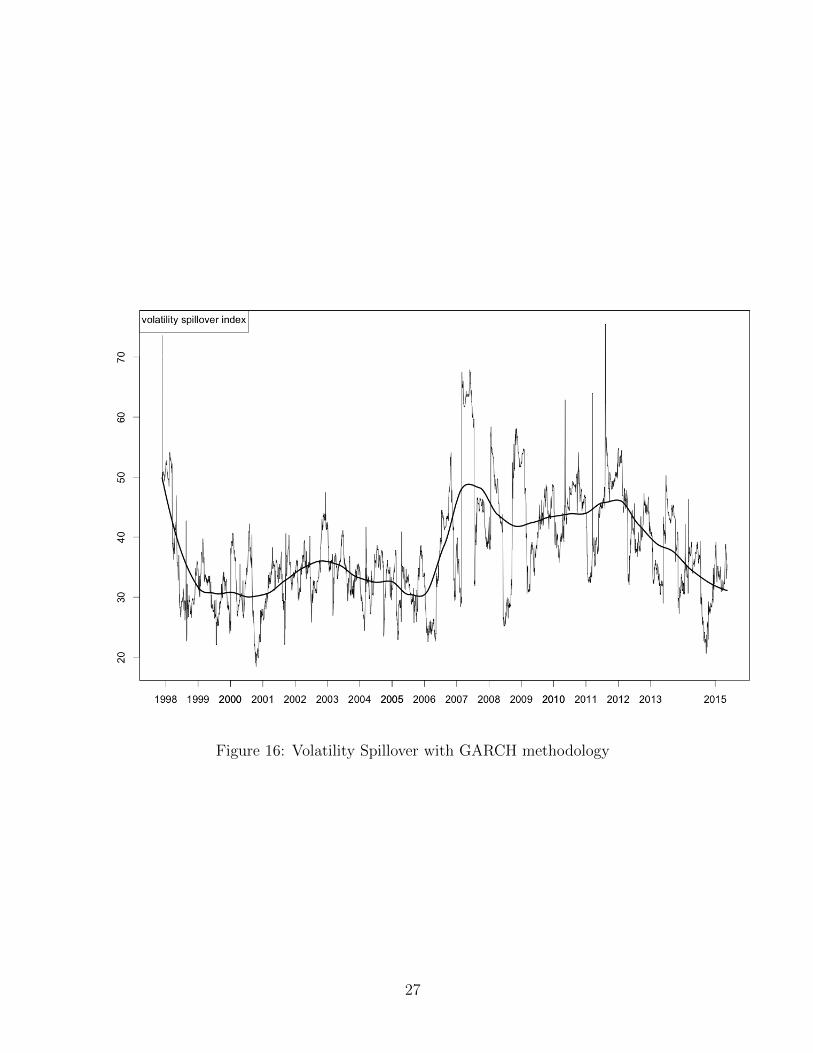
Figure 16: Volatility Spillover with GARCH methodology
27
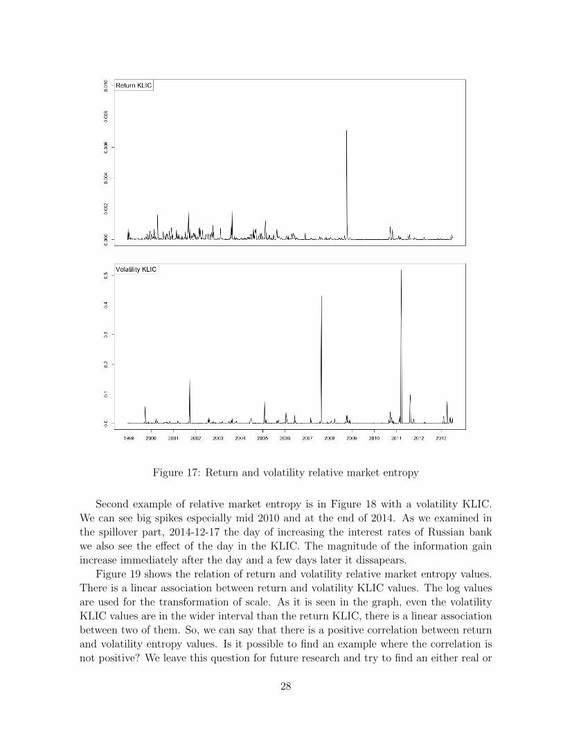
Figure 17: Return and volatility relative market entropy
Second example of relative market entropy is in Figure 18 with a volatility KLIC.
We can see big spikes especially mid 2010 and at the end of 2014. As we examined in
the spillover part, 2014-12-17 the day of increasing the interest rates of Russian bank
we also see the effect of the day in the KLIC. The magnitude of the information gain
increase immediately after the day and a few days later it dissapears.
Figure 19 shows the relation of return and volatility relative market entropy values.
There is a linear association between return and volatility KLIC values. The log values
are used for the transformation of scale. As it is seen in the graph, even the volatility
KLIC values are in the wider interval than the return KLIC, there is a linear association
between two of them. So, we can say that there is a positive correlation between return
and volatility entropy values. Is it possible to find an example where the correlation is
not positive? We leave this question for future research and try to find an either real or
28

Figure 18: Volatility relative market entropy for the case of Example 2 (with Russia)
29

hypothetical example where the correlation is not positive.
- KS entropy:
There is an another type of entropy measure which is explained in Section 2.2 as
a Kolmogorov-Sinai entropy measure. Demetrius [1], introduced this entropy measure
in population theory and Schmidbauer, Rosch and Uluceviz [8] adjust it in the field of
market connectedness. The idea that is developed by Schmidbauer, Rosch and Uluce-
viz [8] is the answer to this question: How the speed of convergence to a news balance
between markets changed across time if the system is distorted by a shock (news)? In
other words, KS entropy measure the speed of information digestion. The KS entropy
for return and volatility is shown in Figure 20.
The overall patterns of KS entropy and spillover index are similar, both for returns
and volatilities. This relation can be seen by comparing the Figure 20 and Figure 11.
The volatility KS entropy is higher then the return KS entropy until 2006, then they
overlap. We have seen a similar behavior in the case of return and volatility spillover
indexes. Both return and volatility KS entropies are in their peak values on October
2008 until September 2010 and then both of them decreased sharply. The similar peak
dates can be seen in the case of return and volatility spillover indexes.
Figure 21 shows the pattern of return and volatility KS entropies. The points show
the return KS entropy in the x-axis and volatility KS entropy in the y-axis. There is a
positive correlation in the return and volatility KS entropy, and volatility KS entropy
value is generally higher then the return KS entropy.
The specific events that we have discussed in Section ?? in terms of the spillover
perspective can also be adopted to the KS entropy for returns and volatilities. There are
similarities between Figure 21 and Figure 12. Some outlier values are in similar dates in
KS entropy and spillover index.
5.2 Part II: Market Connectedness: The Case of Turkey
We show in Section 5.1 how to apply the methodology of return and volatility spillovers
using the five stock market. In this section, our goal is to present an investigation about
the connectedness of Turkish stock market and to measure it using a new methodology
than in Section 2. For now, we only look at the return-to-volatility spillovers using the
weekly return series of the stock market. We leave the volatility spillover in case of
Turkey part as a future work of this thesis.
Here, instead of using the stock markets alone we have grouped the stock market of
36 countries in terms of an organizations as follows: Turkey, European union countries
(EU), Organization of the Islamic Conference countries (OIC), Brazil, Russia, India and
China as in the group of BRIC, and USA. So, we only leave Turkish stock market alone
to measure the connectedness with the other groups.
The aim of doing this is we try to assess the degree of Turkish connectedness with
other groups of markets, in particular with the OIC countries. Although we use the same
return spillovers methodology like in Section 5.1, we decided to develop the methodology,
30

●
●
●
●
●
●
●
● ●
●
●
●●
●●
●●
●
●●
●●
●
●
●●
●
● ●
●●●
●
●
●
●
●
●
●
●
●
●
●
●
●● ●●
●
●
●
●
●
●
●
●
●
●
●
●
●
●
●
●
●
●
●
●
●
●
●
●●●
●
●●
●
●
●
●
●●
●
●
●
●
●
●
●
●
●●
●
●
●
●
●●
●
●●
●
●
●●
●
●
●
●
●
●●
●
●
●
●
●
●
●
●
● ●
●
●
●
●
●
●●
●
●
●●
●
●
●
●
●
●
●
●
●
●
●
●
●●
●
●
●
●
●
●
●
●
●
●
●
●
●
●
●
●
●
●
●
●
●
●
●
●
●●
●●
●
●
●● ●
●
●
●
●
●
●●
●
●
●
●
●
●
●●
●
●
●
●
●
●
●
●
●
●
●
●
●
●
●
●
●
●
●
●
●
●●
●
●
●
●
●
●
●
●
●●
●●
●
●
●
●●
●
●
●
●
●
●
●
●
●
●
●
●
●
●
●
●
● ●
●
●
●
●
● ●
●
●
●
●
●
●
●
●
●●
● ●
●
●
●
●
●
●
●
●
●●
●●
●
●
●●
●
● ●
●
●
●
●
●
●●
●
●
●
●
●
●
●
●●
●
●
● ●
●
●
●
●
●
●●
●
●
●
●
●
●
●●
● ●●
●
●●
●●
●
●
●
●
●
●
●
●
●
●
●
●
●●
●
●
●
●
●●
●
●●
●
●
●
●
●
●
●
●
●
●
●
●●
●
●●
●
●
●
●
●
●●
●
●
●●
●
●
●
●
●
●
●
●
●
●
●
●
●●
●●
●
●
●
●
●
●
●
●
●●
●●
●
●
●
●
●
●
●
●
●
●
●
●
●
●
●
●
●
●
●
●
● ●
●
●
●
●
●
●
●
●
●
●
●
●
●
●●
●
●
●
●
●
●
●
●
●
●
●
●
●
●
● ●●
●
●
●
●
●
●
●
●
●
●
●
●
●
●
●
●
●
●
●
●
●
●
●
●
●
●
●
●
●
●
●
●
●
●
●
●
●
●
●
●
●
●
●
●●
●
●●
●
●
●
●
●
●
●
●
●
●
●
●
●
●
●
●
●
●
●●
●
●
●
●
●
●
●
●
●
●
●
●●
●
●
●
●
●
●
●
●
●
●
●
●
●
●
●
●
●
●
●
●
●
●
●●
●
●
●
●
●
●●●
●●
●
●●
●●
●
●
●
●
●
●
●
●
●
●●
●
●
●
●●●
●
●
●
●
●
●
●
●
●
●
●
●
●
●
●
●
●
●
●
●
●
●
●
●
●
●●
●
●
●
●●
●
●
●
●
●
●
●
●●
●
●●
●
●●
●
●
●
●
●
●
●
●
●
●
●●
●
●●
●
●
●
●
●
●
●
●
●
●
●
●
●
●
●●●
●
●
●
●●
●
●
●
●
● ●
●
●
●
●
●●
●
●
●●
●
●
●
●
●
●
●
●●
●
●●
●
●●
●
●
●
●
●
●
●
●●
●
●
●
●
●
●
●●
●
● ●
●●
●
●
●
●
●
●
●
●
●
●
●
●
●
●
●
●
●
●
●
●
●
−16 −14 −12 −10 −8 −6
−20
−15
−10
−5
0
Return KLIC
Vol
atili
ty K
LIC
log KLIC
Figure 19: Return vs volatility relative market entropy
31

Figure 20: Return and volatility KS entropy
because there are problems while we use different stock market groups instead of taking
every market separately. We again consider a directed network with equity markets as
nodes and return-to-volatility spillovers, obtained via forecast error variance decomposi-
tions (fevd) as the weights of the edges. But, when other markets are grouped together
(such as stock markets within the EU), it is not meaningful to simply add up percent-
ages across markets in each group, because groups are unequally large, the number of
countries is not the same in every group, and so by simply adding up percentages leads
an exaggeration of large groups’ influence. Thus, we developed the methodology and
first summarize the series within each group using principal component analysis and
subsequently decide which series to include by comparison with white noise. We leave
the theoretical detailed explanation of the developed methodology as a next study of the
thesis. In Figure 22 we showed the return spillovers to Turkey from four different groups
that we mentioned above and Turkey itself.
So, we can see that last ten years the return spillovers from Turkey to Turkey itself
increased a lot in the last five years. It means the share of spillovers originating from
outside to the local stock market is decreasing and Turkey is affected more from itself.
We can also conclude that the spillover from OIC to Turkey is also increased which
might be interpret as Turkey started to be more connected to the Islamic countries than
before. As a future study, using the notions related to the network centrality and add
information entropy to this study, we can also identify political and economic events
32

●●●●
●
●● ●● ●●●● ●●●● ●●
●●●●● ●●●● ● ●●● ●●●● ●●●● ●●
● ●●
●
●
●●
●●
● ● ●●●●
●●●●
●●
●
●
●
●
●●●
●
●●
●●●
● ●●●●
●● ●
●
●
●
●●
●
●●
●
●●●
●●
●
●● ●●
●
●●
● ●●
●●●
●
●
●●
● ●
●
● ●
●
●●
●●●●● ●●●●● ●● ●●
●●●
●●●
●
●
●
●
●● ●●●
●●
●● ● ●
● ●
●●●
●●
●● ●
●
● ●●
●●
●●●● ●●●
●●●●●
●
●
●
●
●●●
●
●●
●
●●
●
●
●
●●
●
●●
● ●●●●●●●●
●
●●
●
●
●
●●●●●●●●●●● ●●●
●
●●●●●●●
●●●●● ●
●
●
●●
●●●●●●●●
●●●●●●
●●●●●
●●●●●●●
●●●●●●
●
●
●●
●●
●●
● ●●
●
●●●●● ●
●●
●
●●
●●● ● ●●
●●
●●●
●
●
●
● ●●●●
● ● ●
●●●●●
●●●●● ●
●●●●●●●
●
●●
●
●●
●
●●
●
●●●●●●
●●● ●●
●
●
●
●
●
●●
● ●●
●
●
●
●
●●
●
●
●●
●
●
●
●●
●● ●●● ●● ●●●●
●
●●●●●●●
●●●●●●●●●●●●
●●
●●●
●●●●●●●●●●
●●●●●●●●●●
●
●
●●●●●●●●●●● ●●
●
●●
●●● ● ●
●●
●●●●●●
●
●
●●●●●●●●
●●
●●●●●●●
●●●●●● ●●●
●●
●
●●●●●
●
●●●●●●●●●●●●●●●●●●●●●●●●●●●●●●●●●●●●●●●●●●●●●●●●●●●●●●●
●
●●●●●●●●●●●●●●●●●●●
●●●●●●●●●●●●●●●
●●
●●●
●
●
●
●
●●
●●●●●
●●
●●
●● ●●
●●
●
●
●●
●
●●●●●●●●●●●
●●●●● ●●●
●
●
●●●●
●●●●
●● ●●●●● ●●●●●●●●●●●●●●●●●
●●●●●●●●●●●●●●●●●
●●●●●●●●●●●●●●●●●●●●●●●●●●●●
●●
●●●●●●
●
●●●●●●
●●
●
●●
●
●●
1.9 2.0 2.1 2.2 2.3
1.9
2.0
2.1
2.2
2.3
Return KS
Vol
atili
ty K
S
KS Entropy
Figure 21: Return vs volatility KS entropy
33

Figure 22: The Case of Turkey
having a big impact on the distribution and origin of stock market volatility in Turkey.
6 Conclusion and Further Research
The first goal of the present study was to compare the results of market connectedness
using the spillover and information flow perspective when the return prices and volatili-
ties of them are used. Using both expectation of stock prices and the variations of them,
gave us an information about how these two complement each other. So, we analyzed
the market with respect to different structures.
We applied spillover and entropy methodologies on expectations of prices and vari-
ations of them. Firstly, we compared the return spillovers and volatility spillovers. We
reached the result that even the return and volatility spillovers behave similarly and there
is a positive correlation among them, at some specific time intervals return spillover and
volatility spillover act different. We tried to explain these results in terms of a “crisis”
or an important event from the history.
The results obtained from KLIC and KS entropy showed us the information gain
comes from either using the return or volatility series. In the KLIC results, the amount
of information created week to week had different pattern in the case of return than the
volatility. The spikes from the volatility is higher than the spikes coming from return.
The magnitude of the information created has been increasing for volatility but in the
34

return there are time intervals where information created has been decreasing.
There is a positive correlation between the values of return market entropy and
volatility market entropy. In the further research of this study we will examine the
reason of this correlation and try to find an example where there is no correlation or the
correlation is negative. Since, it is not obvious that we can find a real example for this,
we will construct a hypothetical example where the correlation is negative among the
return KLIC and volatility KLIC. Therefore, we can compare the information created in
these two cases where there is positive and negative correlations.
In the case of KS entropy, the similar situation like in the spillover index have found.
There is a relation in the return and volatility KS entropies, but at some specific time
intervals the volatility KS entropy, which gives us an information about the shock di-
gestion, is higher than the return KS. We tried to explain the reasons as we did in the
spillover index. We will improve the entropy idea in the future study of the thesis and
examine the results in terms of economics events. Also, we will try to find a link among
the spillover methodology and the entropy.
Then, since we have used the weekly return and weekly volatility series, we needed to
obtain the weekly return and volatilities using daily data. We followed the methodology
of German and Klass [14] to construct the weekly volatility series and tried to understand
the intuition behind the method. So, both spillover and information flow perspective
depended on the weekly return and volatility series that we have obtained. We have
also used the GARCH methodology to obtain the volatility series and we compared the
results with German and Klass methodology. We have used a new stock market data
group to examine the different effects and compare the two methodologies calculating
the volatility spillovers. In our further study, we will develop the idea and also try to
find the best methodology of volatility estimation for our study.
The second goal was to measure the connectedness of Turkey using a new methodol-
ogy of return spillovers. We conclude that the spillovers from Turkey to Turkey increased
in the last five years. We will interpret the reasons of this increase in the future studies
and try to find an economic interpretation of them. We will also examine the change
in the relation between Turkey and Islamic countries based on the OIC countries. After
completing the return spillovers part we will apply the new methodology in the case of
Turkey using the volatility spillover method. This will be an important contribution
since due to the different interpretations of return and volatility spillovers we will under-
stand the change in the connectedness in Turkey using the stock market and interpret
the Turkish economy in the last decade. We will also add the entropy methodology in
addition to the spillover one and try to examine the market and understand the effects
of information and the digestion of them in the economy.
We would like to mention that the present paper have been submitted and accepted
for presentation at the Ecomod conference, in Boston, United States, in July 2015.
35

References
[1] Demetrius, L. (1974): Demographic parameters and natural selection, Proc. Natl.
Acad. Sci. USA, 71, 4645–4647.
[2] Diebold, F.X., and K. Yilmaz (2009): Measuring Financial Asset Return and
Volatility Spillovers, with Application to Global Equity Markets, Economic Jour-
nal , 119, 158–171.
[3] Diebold, F.X., and K. Yilmaz (2013): On The Network Topology of Variance
Decompositions: Measuring The Connectedness of Financial Firms, Journal of
Econometrics , forthcoming.
[4] International Monetary Fund, ed. (2012). 2012 Spillover Report — Background
Papers, Washington, DC, U.S.A.: International Monetary Fund.
[5] Kolmogorov, A.N. (1959): Entropy per unit time as a metric invariant of automor-
phism, Doklady of Russian Academy of Sciences , 124, 754–755.
[6] Kullback S., and R.A. Leibler (1951): On Information and Sufficiency, Annals of
Mathematical Statistics , 22, 79–86.
[7] Lutkepohl, H. (2005): New Introduction to Multiple Time Series Analysis . New
York: Springer.
[8] Schmidbauer H., Rouch A., and Uluceviz E., 2012: Understanding market
connectedness: A Markov chain approach, Available online at http://www.hs-
stat.com/projects/papers/schmidbauer roesch uluceviz connectedness mc approach
v2012-09-14.pdf.
[9] Pesaran H.H., and Y. Shin (1998): Generalized Impulse Response Analysis in
Linear Multivariate Models, Economics Letters , 58, 17–29.
[10] Rigobon, R. (2001): Contagion: How to Measure it? In Preventing Currency
Crises in Emerging Markets, ed. by S. Edwards, and J.A. Frankel. Chicago: The
University of Chicago Press.
[11] Rigobon, R. (2002): International Financial Contagion: Theory and Evidence in
Evolution, Charlottesville (VA), U.S.A: The Research Foundation of AIMR.
[12] Stock, J.H., and M. Watson (2003): Has the Business Cycle Changed and Why? In
NBER Macroeconomics Annual 2002, ed. by M. Gertler, and K. Rogoff. Cambridge
(MA), U.S.A.: The MIT Press.
[13] Tuljapurkar, S.D. (1982): Why use population entropy? It determines the rate of
convergence, J. Math. Biology , 13, 325–337.
36

[14] German, M.B. and Klass, M.J. (1980): On the estimation of security price volatil-
ities from historical data, Journal of Business , 53 (1), 67–78.
[15] Alizadeh, S., Brandt, M.W. and Diebold, F.X. (2002): Range-based estimation of
stochastic volatility models, Journal of Finance, 57 (3), 1047-92.
37