market basket analysis for data mining by mehmet aydın
TRANSCRIPT

MARKET BASKET ANALYSIS FOR DATA MINING
by
Mehmet Aydın Ulas
BS. in Computer Engineering, Bogazici University, 1999
Submitted to the Institute for Graduate Studies in
Science and Engineering in partial fulfillment of
the requirements for the degree of
Master of Science
in
Computer Engineering
Bogazici University
2001
ii
MARKET BASKET ANALYSIS FOR DATA MINING
APPROVED BY:
Assoc. Prof. A. I. Ethem Alpaydın . . . . . . . . . . . . . . . . . . .
(Thesis Supervisor)
Assoc. Prof. Taner Bilgic . . . . . . . . . . . . . . . . . . .
Prof. Fikret Gurgen . . . . . . . . . . . . . . . . . . .
DATE OF APPROVAL: 11.06.2001

iii
ACKNOWLEDGEMENTS
I want to thank Ethem Alpaydın for helping me all the time with ideas for my
thesis and for his contribution to my undergraduate and graduate education. I want to
thank Fikret Gurgen and Taner Bilgic for their contribution to my undergraduate and
graduate education and for participating in my thesis jury. I want to thank Dengiz
Pınar, Nasuhi Sonmez and Ataman Kalkan of Gima Turk A.S. for supplying me the
data I used in my thesis. I want to thank my family who always supported me and
never left me alone during the preperation of this thesis.
iv
ABSTRACT
MARKET BASKET ANALYSIS FOR DATA MINING
Most of the established companies have accumulated masses of data from their
customers for decades. With the e-commerce applications growing rapidly, the com-
panies will have a significant amount of data in months not in years. Data Mining,
also known as Knowledge Discovery in Databases (KDD), is to find trends, patterns,
correlations, anomalies in these databases which can help us to make accurate future
decisions.
Mining Association Rules is one of the main application areas of Data Mining.
Given a set of customer transactions on items, the aim is to find correlations between
the sales of items.
We consider Association Mining in large database of customer transactions. We
give an overview of the problem and explain approaches that have been used to attack
this problem. We then give the description of the Apriori Algorithm and show results
that are taken from Gima Turk A.S. a large Turkish supermarket chain. We also
use two statistical methods: Principal Component Analysis and k-means to detect
correlations between sets of items.
v
OZET
VERI MADENCILIGI ICIN SEPET ANALIZI
Bircok gelismis firma yıllar boyunca musterilerinden cok fazla miktarda veri
topladılar. Elektronik ticaret uygulamalarının da cogalmasıyla sirketler artık cok fazla
veriyi yıllar degil aylarla olculebilecek bir zamanda bir araya getirebiliyorlar. Verita-
banlarında Bilgi Kesfi olarak da bilinen Veri Madenciliginin amacı ilerki asamalardaki
kararlara yardımcı olması icin veri icerisinde yonsemeler, oruntuler, ilintiler ve sapak-
lıklar bulmaktır.
Iliski Kuralları Bulma Veri Madenciliginin ana uygulama alanlarından bir tane-
sidir. Sepet analizinin amacı verilen bir satıs raporları uzerinden mallar arasında ilin-
tiler bulmaktır.
Bu tezde genis bir mal satıs veri tabanı uzerinde Iliski Madenciligi calısması
yaptık. Ilk kısımda problemin genel hatlarla tanımını ve bu problemi cozmek icin
kullanılan yaklasımları anlattık. Bu konuda ilk kullanılan algoritmalardan birisi olan
“Apriori Algoritması” nı detaylı olarak inceleyerek bu algoritmanın buyuk bir super-
market zinciri olan Gima Turk A.S.’nin verileri uzerinde uygulanmasıyla ortaya cıkan
sonucları verdik. Ayrıca mal satısları arasında ilintiler bulmak icin iki istatistiksel
method kullandık: Ana Bilesen Analizi ve k-Ortalama Obeklemesi.
vi
TABLE OF CONTENTS
ACKNOWLEDGEMENTS . . . . . . . . . . . . . . . . . . . . . . . . . . . . . iii
ABSTRACT . . . . . . . . . . . . . . . . . . . . . . . . . . . . . . . . . . . . . iv
OZET . . . . . . . . . . . . . . . . . . . . . . . . . . . . . . . . . . . . . . . . . v
LIST OF FIGURES . . . . . . . . . . . . . . . . . . . . . . . . . . . . . . . . . vii
LIST OF TABLES . . . . . . . . . . . . . . . . . . . . . . . . . . . . . . . . . . ix
LIST OF SYMBOLS/ABBREVIATIONS . . . . . . . . . . . . . . . . . . . . . xi
1. INTRODUCTION . . . . . . . . . . . . . . . . . . . . . . . . . . . . . . . . 1
1.1. Formal Description of the Problem . . . . . . . . . . . . . . . . . . . . 2
1.2. Outline of Thesis . . . . . . . . . . . . . . . . . . . . . . . . . . . . . . 7
2. METHODOLOGY . . . . . . . . . . . . . . . . . . . . . . . . . . . . . . . . 13
2.1. Algorithm Apriori . . . . . . . . . . . . . . . . . . . . . . . . . . . . . . 13
2.1.1. Finding Large Itemsets . . . . . . . . . . . . . . . . . . . . . . . 13
2.1.1.1. Itemset Generation . . . . . . . . . . . . . . . . . . . . 13
2.1.1.2. Pruning . . . . . . . . . . . . . . . . . . . . . . . . . . 14
2.1.2. Generating Rules . . . . . . . . . . . . . . . . . . . . . . . . . . 15
2.1.2.1. Rule Generation . . . . . . . . . . . . . . . . . . . . . 15
2.2. Principal Component Analysis . . . . . . . . . . . . . . . . . . . . . . . 16
2.3. k-Means Clustering . . . . . . . . . . . . . . . . . . . . . . . . . . . . . 18
3. RESULTS . . . . . . . . . . . . . . . . . . . . . . . . . . . . . . . . . . . . . 21
3.1. Description of Datasets . . . . . . . . . . . . . . . . . . . . . . . . . . . 21
3.2. Large Items . . . . . . . . . . . . . . . . . . . . . . . . . . . . . . . . . 21
3.3. Rules Generated . . . . . . . . . . . . . . . . . . . . . . . . . . . . . . 22
3.4. Finding Correlations Using PCA . . . . . . . . . . . . . . . . . . . . . 22
3.5. Clustering Customers Using k-Means . . . . . . . . . . . . . . . . . . . 27
4. CONCLUSIONS AND FUTURE WORK . . . . . . . . . . . . . . . . . . . . 33
APPENDIX A: RESULTS OF PRINCIPAL COMPONENT ANALYSIS . . . 35
APPENDIX B: RESULTS OF K-MEANS CLUSTERING . . . . . . . . . . . 53
REFERENCES . . . . . . . . . . . . . . . . . . . . . . . . . . . . . . . . . . . . 61
REFERENCES NOT CITED . . . . . . . . . . . . . . . . . . . . . . . . . . . . 63
vii
LIST OF FIGURES
Figure 1.1. Finding large itemsets . . . . . . . . . . . . . . . . . . . . . . . . . 8
Figure 1.2. Sampling Algorithm . . . . . . . . . . . . . . . . . . . . . . . . . . 9
Figure 1.3. Partition Algorithm . . . . . . . . . . . . . . . . . . . . . . . . . . 9
Figure 1.4. Mining N most interesting itemsets . . . . . . . . . . . . . . . . . 10
Figure 1.5. Adaptive Parallel Mining . . . . . . . . . . . . . . . . . . . . . . . 11
Figure 1.6. Fast Distributed Mining of association rules with local pruning . . 12
Figure 2.1. Algorithm Apriori . . . . . . . . . . . . . . . . . . . . . . . . . . . 14
Figure 2.2. Candidate generation . . . . . . . . . . . . . . . . . . . . . . . . . 16
Figure 2.3. Pruning . . . . . . . . . . . . . . . . . . . . . . . . . . . . . . . . 17
Figure 2.4. Generating rules . . . . . . . . . . . . . . . . . . . . . . . . . . . . 19
Figure 2.5. Random initial start vectors for k = 4 . . . . . . . . . . . . . . . . 20
Figure 2.6. Final means for k = 4 . . . . . . . . . . . . . . . . . . . . . . . . . 20
Figure 3.1. Energy and data reduced to 2 dimensions for 25 items for store
number 102 . . . . . . . . . . . . . . . . . . . . . . . . . . . . . . 32
Figure A.1. Energy and data reduced to 2 dimensions for 25 items for store
number 221 . . . . . . . . . . . . . . . . . . . . . . . . . . . . . . 42
viii
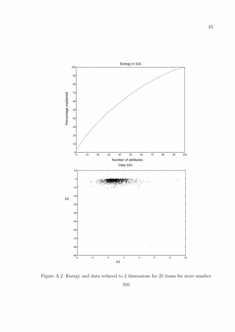
Figure A.2. Energy and data reduced to 2 dimensions for 25 items for store
number 310 . . . . . . . . . . . . . . . . . . . . . . . . . . . . . . 43
Figure A.3. Energy and data reduced to 2 dimensions for 25 items for whole data 44
Figure A.4. Energy and data reduced to 2 dimensions for 46 items for store
number 102 . . . . . . . . . . . . . . . . . . . . . . . . . . . . . . 45
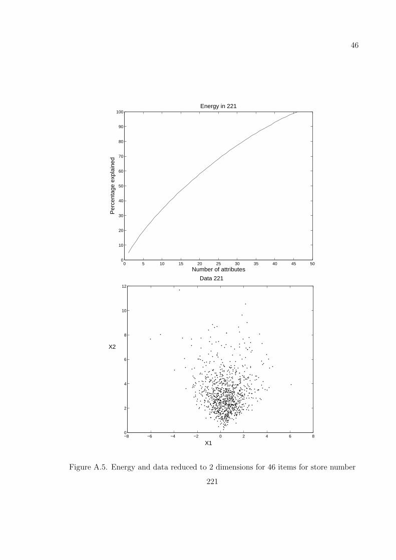
Figure A.5. Energy and data reduced to 2 dimensions for 46 items for store
number 221 . . . . . . . . . . . . . . . . . . . . . . . . . . . . . . 46
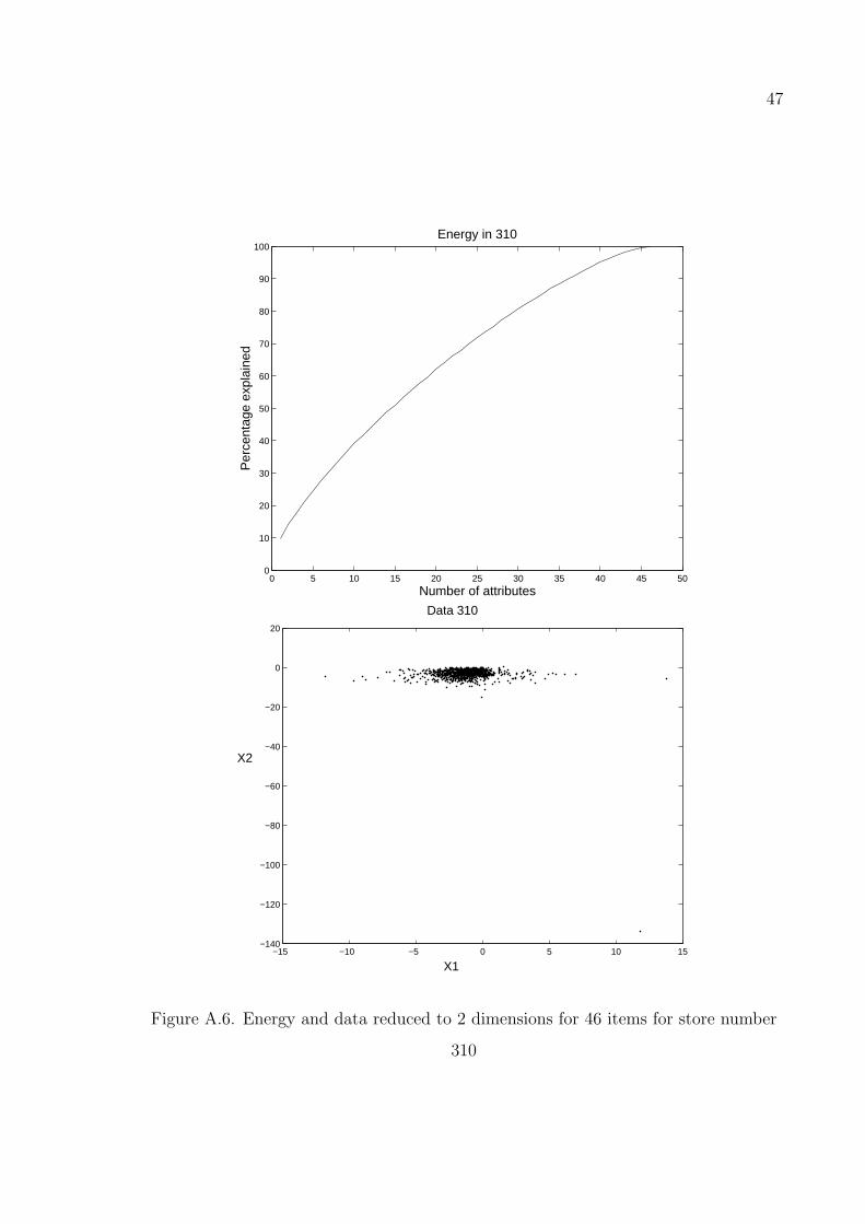
Figure A.6. Energy and data reduced to 2 dimensions for 46 items for store
number 310 . . . . . . . . . . . . . . . . . . . . . . . . . . . . . . 47
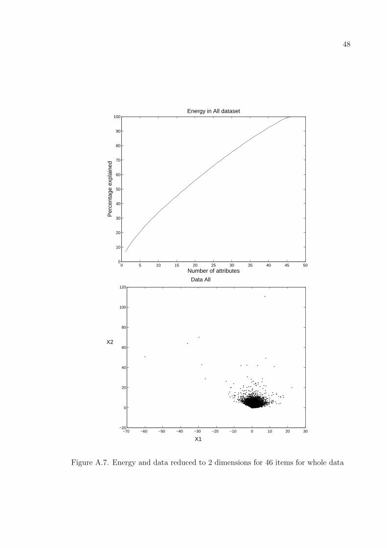
Figure A.7. Energy and data reduced to 2 dimensions for 46 items for whole data 48
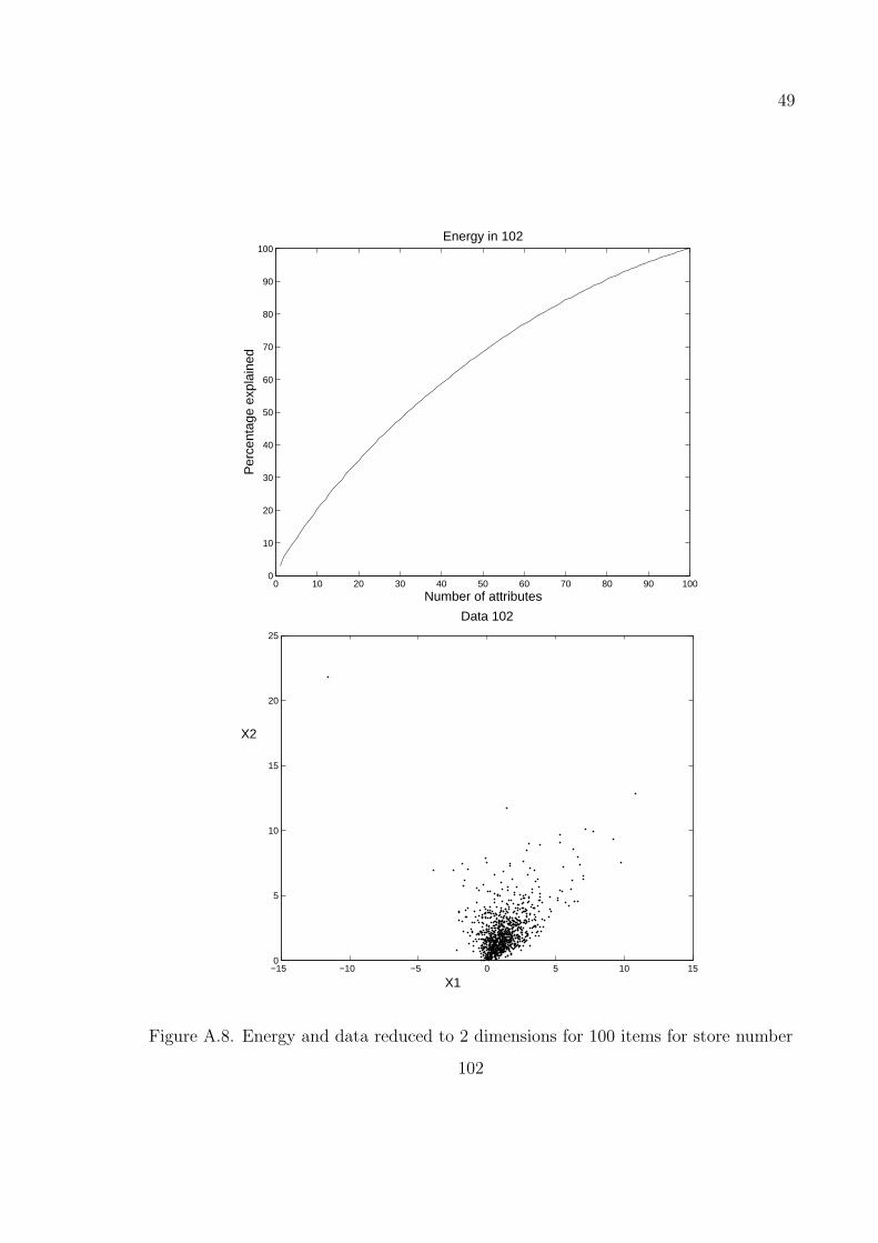
Figure A.8. Energy and data reduced to 2 dimensions for 100 items for store
number 102 . . . . . . . . . . . . . . . . . . . . . . . . . . . . . . 49
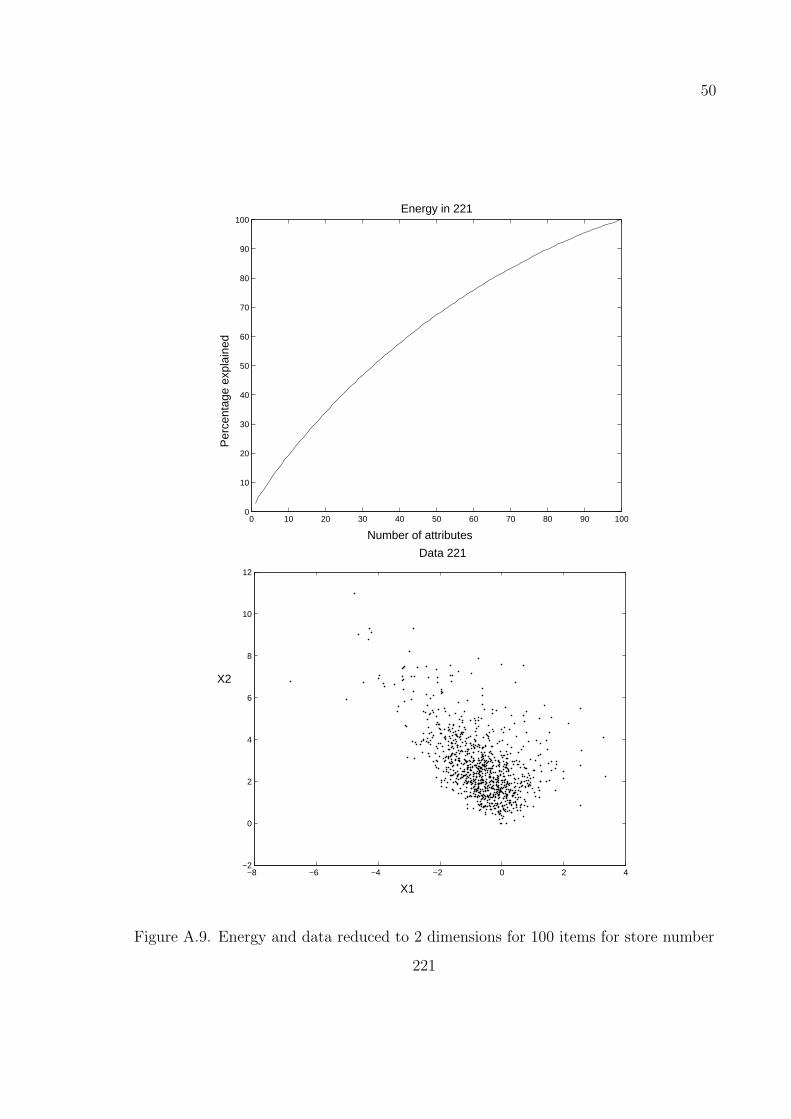
Figure A.9. Energy and data reduced to 2 dimensions for 100 items for store
number 221 . . . . . . . . . . . . . . . . . . . . . . . . . . . . . . 50
Figure A.10. Energy and data reduced to 2 dimensions for 100 items for store
number 310 . . . . . . . . . . . . . . . . . . . . . . . . . . . . . . 51
Figure A.11. Energy and data reduced to 2 dimensions for 100 items for whole
data . . . . . . . . . . . . . . . . . . . . . . . . . . . . . . . . . . 52
ix
LIST OF TABLES
Table 2.1. Example of Apriori . . . . . . . . . . . . . . . . . . . . . . . . . . 15
Table 3.1. Table Fis Baslik used in the datasets . . . . . . . . . . . . . . . . . 21
Table 3.2. Table Fis Detay used in the datasets . . . . . . . . . . . . . . . . . 22
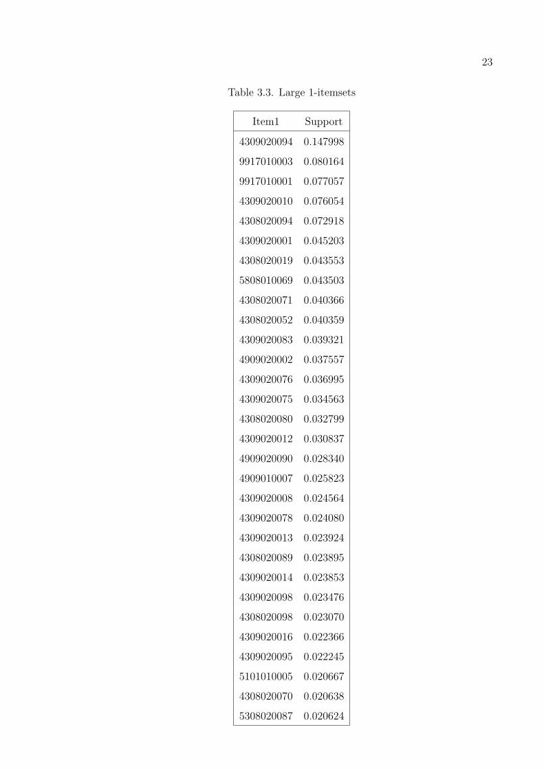
Table 3.3. Large 1-itemsets . . . . . . . . . . . . . . . . . . . . . . . . . . . . 23
Table 3.4. Large 2-itemsets . . . . . . . . . . . . . . . . . . . . . . . . . . . . 24
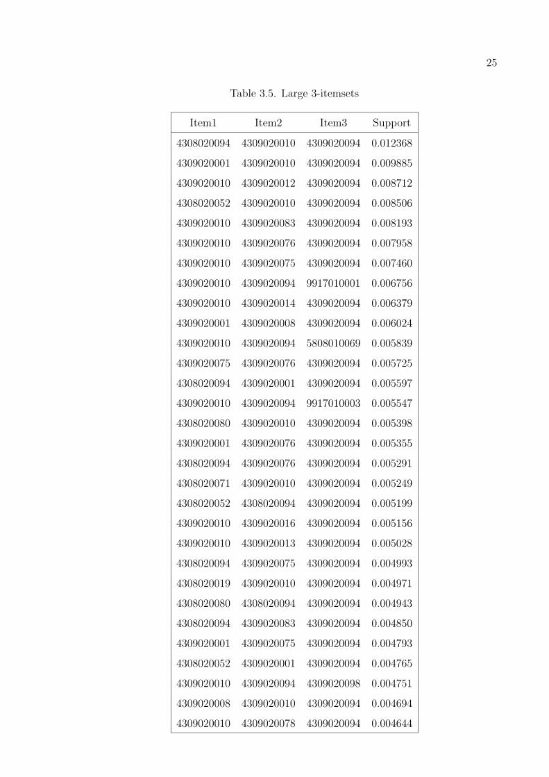
Table 3.5. Large 3-itemsets . . . . . . . . . . . . . . . . . . . . . . . . . . . . 25
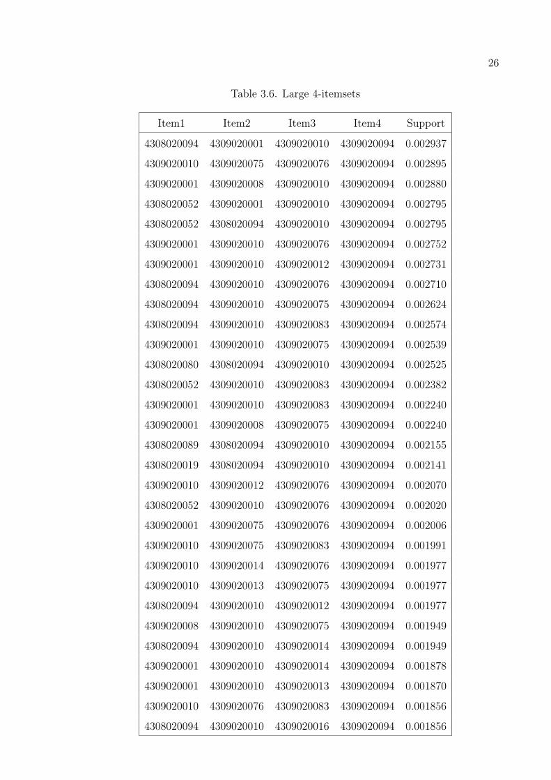
Table 3.6. Large 4-itemsets . . . . . . . . . . . . . . . . . . . . . . . . . . . . 26
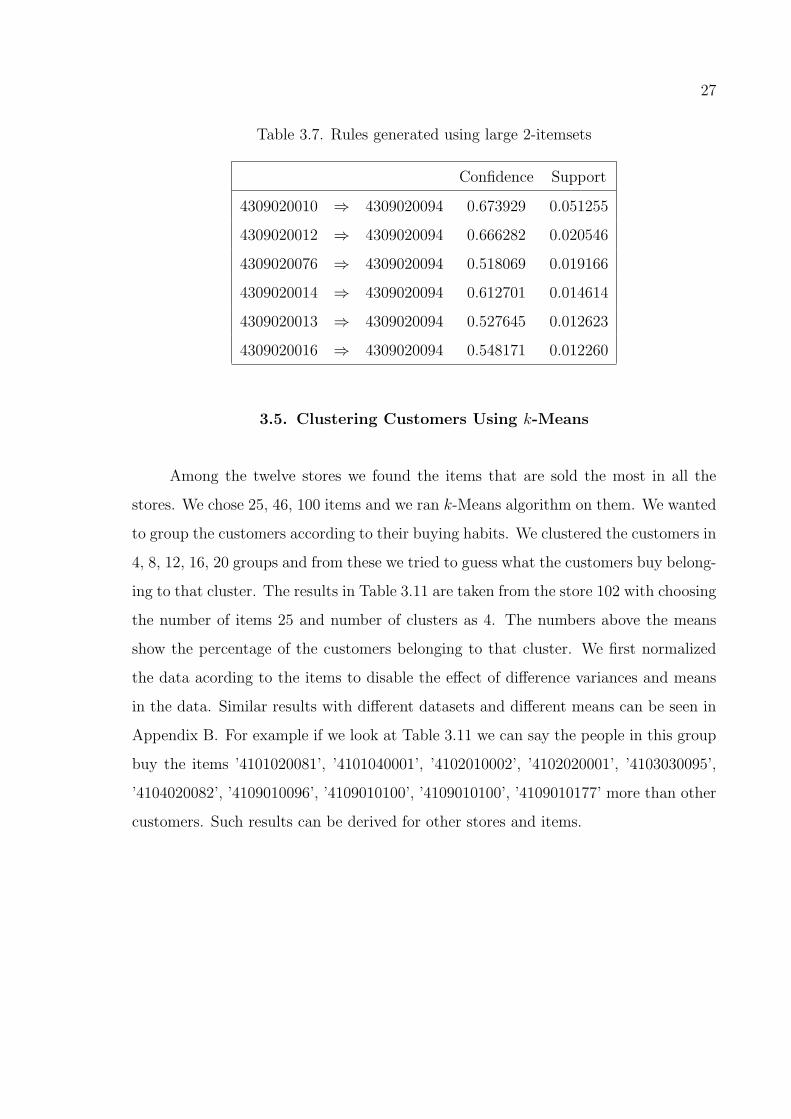
Table 3.7. Rules generated using large 2-itemsets . . . . . . . . . . . . . . . . 27
Table 3.8. Rules generated using large 3-itemsets . . . . . . . . . . . . . . . . 28
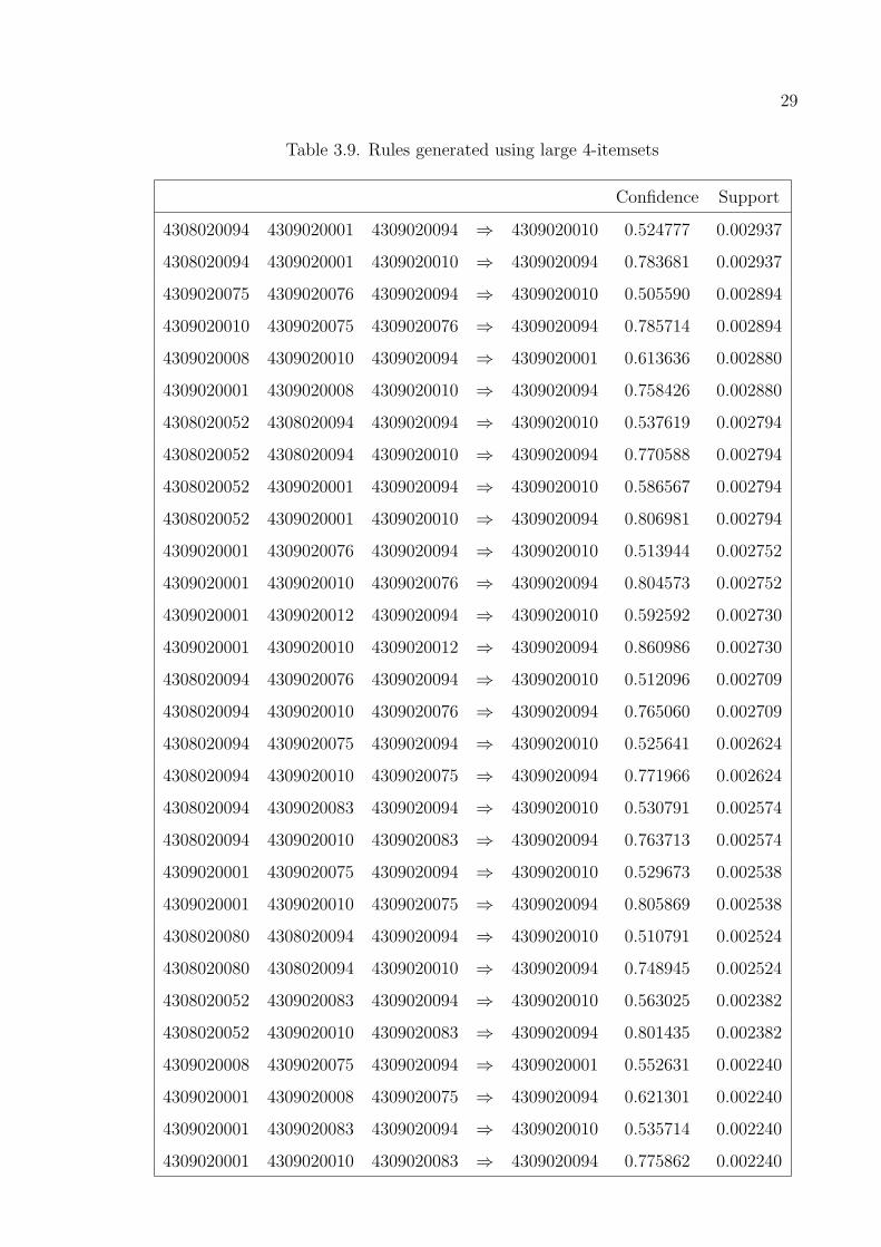
Table 3.9. Rules generated using large 4-itemsets . . . . . . . . . . . . . . . . 29
Table 3.10. Energies in 25 dimensions . . . . . . . . . . . . . . . . . . . . . . . 30
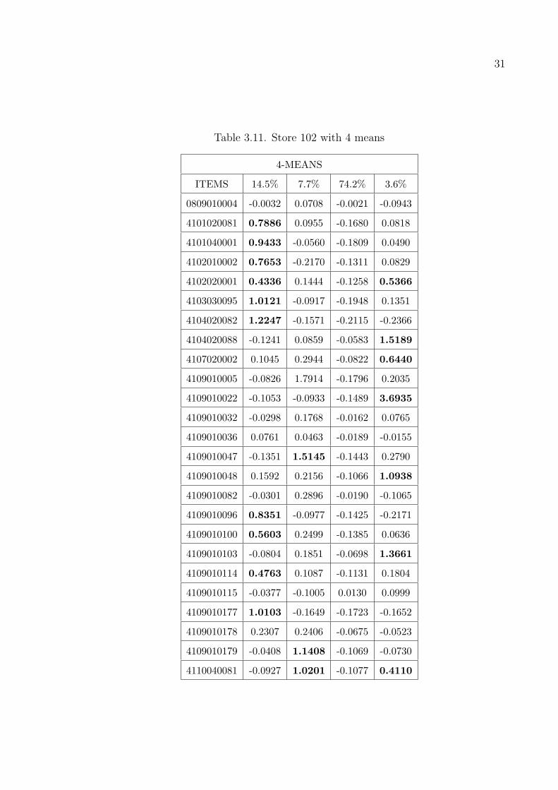
Table 3.11. Store 102 with 4 means . . . . . . . . . . . . . . . . . . . . . . . . 31
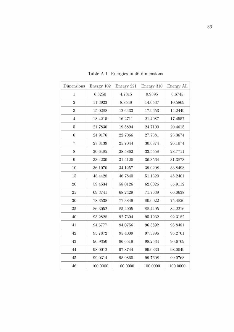
Table A.1. Energies in 46 dimensions . . . . . . . . . . . . . . . . . . . . . . . 36
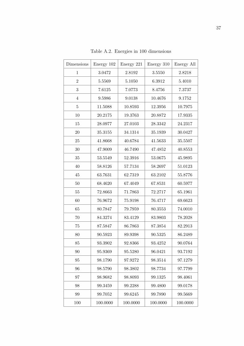
Table A.2. Energies in 100 dimensions . . . . . . . . . . . . . . . . . . . . . . 37
Table A.3. Eigenvectors for 25 dimensions reduced to 6 dimensions for store 102 38

x
Table A.4. Eigenvectors for 25 dimensions reduced to 6 dimensions for store 221 39
Table A.5. Eigenvectors for 25 dimensions reduced to 6 dimensions for store 310 40
Table A.6. Eigenvectors for 25 dimensions reduced to 6 dimensions for all data 41
Table B.1. Store 102 with 8 means . . . . . . . . . . . . . . . . . . . . . . . . 54
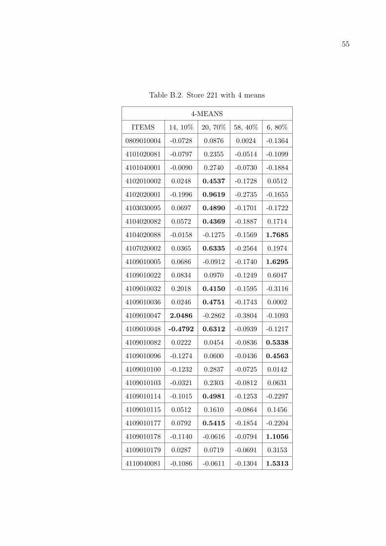
Table B.2. Store 221 with 4 means . . . . . . . . . . . . . . . . . . . . . . . . 55
Table B.3. Store 221 with 8 means . . . . . . . . . . . . . . . . . . . . . . . . 56
Table B.4. Store 310 with 4 means . . . . . . . . . . . . . . . . . . . . . . . . 57
Table B.5. Store 310 with 8 means . . . . . . . . . . . . . . . . . . . . . . . . 58
Table B.6. All stores with 4 means . . . . . . . . . . . . . . . . . . . . . . . . 59
Table B.7. All stores with 8 means . . . . . . . . . . . . . . . . . . . . . . . . 60
xi
LIST OF SYMBOLS/ABBREVIATIONS
btj 1 if xt belongs to cluster j, 0 otherwise
D The whole database
DBi The database at the ith distributed site
|D| Size of the database
E[x] Expected value of x
vj The jth cluster center
xt The tth input vector
η Learning Factor
λi ith eigenvalue
AI Artificial Intelligence
APM Adaptive Parallel Mining
CRM Customer Relationship Management
FDM Fast Distributed Mining of association rules
KDD Knowledge Discovery in Databases
OS Operating System
PCA Principal Component Analysis
1
1. INTRODUCTION
Data Mining, also known as Knowledge Discovery in Databases (KDD), is to
find trends, patterns, correlations, anomalies in these databases which can help us
to make accurate future decisions. However data mining is not magic. No one can
guarantee that the decision will lead to good results. Data Mining only helps experts
to understand the data and lead to good decisions. Data Mining is an intersection of
the fields Databases, Artificial Intelligence and Machine Learning. Some examples of
Data Mining applications are:
• Market Basket Analysis (Association Mining). It is the main focus of this
thesis. Market Basket Analysis is the discovery of relations or correlations among
a set of items.
• Classification. Classification analyzes a training set of objects with known
labels and tries to form a model for each class based on the features in the data.
• Regression. Regression is to predict values of some missing data or to build a
model for some attributes using other attributes of the data.
• Time Series Analysis. Time Series Analysis is to analyze time series data to
find certain regularities and interestingness in data.
• Clustering. Clustering is to identify clusters embedded in the data. The task is
to find clusters for which inter-cluster similarity is low and intra-cluster similarity
is high.
• Outlier Analysis. Outlier analysis is to find outliers in the data, namely detect
data which are very far away from average behaviour of the data.
Recent work focuses mostly on scaling Data Mining algorithms. An algorithm is
said to be scalable if its runtime increases linearly with the number of records in the
input database. In general, a Knowledge Discovery Process consists of the following
steps:
• Data cleaning, which handles noisy, erroneous, missing or irrelevant data
2
• Data integration, where data sources are integrated into one
• Data selection, where relevant is selected from the database
• Data transformation, where data is formed into appropriate format for mining
• Data mining, which is the essential process where intelligent methods are applied
• Pattern evaluation, which identifies patterns using some interestingness measures
• Knowledge presentation, where visualization techniques are used to present the
mined data to the user.
Lately, mining association rules, also called market basket analysis, is one of the
application areas of Data Mining. Mining Association Rules has been first introduced in
[1]. Consider a market with a collection of huge customer transactions. An association
rule is X⇒Y where X is called the antecedent and Y is the consequent. X and Y
are sets of items and the rule means that customers who buy X are likely to buy Y
with probability %c where c is called the confidence. Such a rule may be: “Eighty
percent of people who buy cigarettes also buy matches”. Such rules allows us to
answer questions of the form “What is Coca Cola sold with?” or if we are interested
in checking the dependency between two items A and B we can find rules that have A
in the consequent and B in the antecedent.
The aim is to generate such rules given a customer transaction database. The
algorithms generally try to optimize the speed since the transaction databases are
huge in size. This type of information can be used in catalog design, store layout,
product placement, target marketing, etc. Basket Analysis is related to, but different
from Customer Relationship Management (CRM) systems where the aim is to find the
dependencies between customers’ demographic data, e.g., age, marital status, gender,
and the products.
1.1. Formal Description of the Problem
Let I = (i1, i2, . . . , im) be a set of transactions. Each i is called an item. D is the
set of transactions where each transaction T is a set of items (itemset) such that T⊆I.
Every transaction has a unique identifier called the TID. An itemset having k items is
3
called a k-itemset. Let X and Y be distinct itemsets. The support of an itemset X is
the ratio of the itemsets containing X to the number of all itemsets. Let us define |X|as the number of itemsets containing X and |D| as the number of all items, |X.Y | as
the number of itemsets containing both X and Y . The support of itemset X is defined
as follows:
support(X) =|X||D| (1.1)
The rule X⇒Y has support s if %s of the transactions in D contain X and Y together.
support(X ⇒ Y ) =|X.Y ||D| (1.2)
Support measures how common the itemsets are in the database and confidence mea-
sures the strength of the rule. A rule is said to have confidence c if %c of the transactions
that contains X also contains Y .
confidence(X ⇒ Y ) =support(X.Y )
support(X)(1.3)
Given a set of transactions D the task of Association Rule Mining is to find rules
X ⇒ Y such that the support of the rule is greater than a user specified minimum
support called minsupp and the confidence is greater than a user specified minimum
called minconf. An itemset is called large if its support is greater than minsupp.
The task of Association Rule Mining can be divided into two: In the first phase,
the large itemsets are found using minsupp, and in the second phase, the rules are
generated using minconf.
The algorithms that implement Association Mining make multiple passes over
the data. Most algorithms first find the large itemsets and then generate the rules
accordingly. They find the large itemsets incrementally increasing itemset sizes and
then counting the itemsets to see if they are large or not. Since finding the large
itemsets is the hard part, research mostly focused on this topic.
4
The problem has been approached from different perspectives with several al-
gorithms. In [1], Agrawal, Imielinski and Swami define the concepts of support and
confidence and give an algorithm which has only one item in the consequent. The
algorithm makes multiple passes over the database. The frontier set for a pass consists
of those itemsets that are extended during a pass. At each pass, support for certain
itemsets is measured. These itemsets called candidate itemsets, are derived from the
tuples in the database and the itemsets contained in the frontier set. The frontier sets
are created using the 1-extensions of the candidate itemsets in the current pass. Figure
1.1 shows the pseudocode for the algorithm.
In [2], Agrawal and Srikant define the algorihms Apriori and AprioriTid which
can handle multiple items in the consequent. We will explain Aprori in detail in Section
2.1 and give real life results taken from data obtained from Gima Turk A.S. that are
obtained using this algorithm in Chapter 3.
An efficient way to calculate the queries that are called iceberg queries is given
by Fang et al. [3]. The queries are used in association mining. An iceberg query
performs an aggregate function over an attribute (or set of attributes) for finding
the aggregate values above some threshold. A typical iceberg query is performed on
a relation R(t1, t2, . . . , tk, ID). An example of an iceberg query can be : SELECT
t1, t2, . . . , tk, count(ID) FROM R GROUPBY t1, t2, . . . , tk HAVING count(ID) > T
In our case t1, t2, . . . , tk correspond to the items and ID corresponds to the ID
of the receipt. They are called iceberg queries because the data we are trying to search
is huge like the iceberg but the results we are going to obtain which are above some
specified threshold are usually very small like the tip of the iceberg. The techniques
are applied if the results are very small compared to the whole dataset.
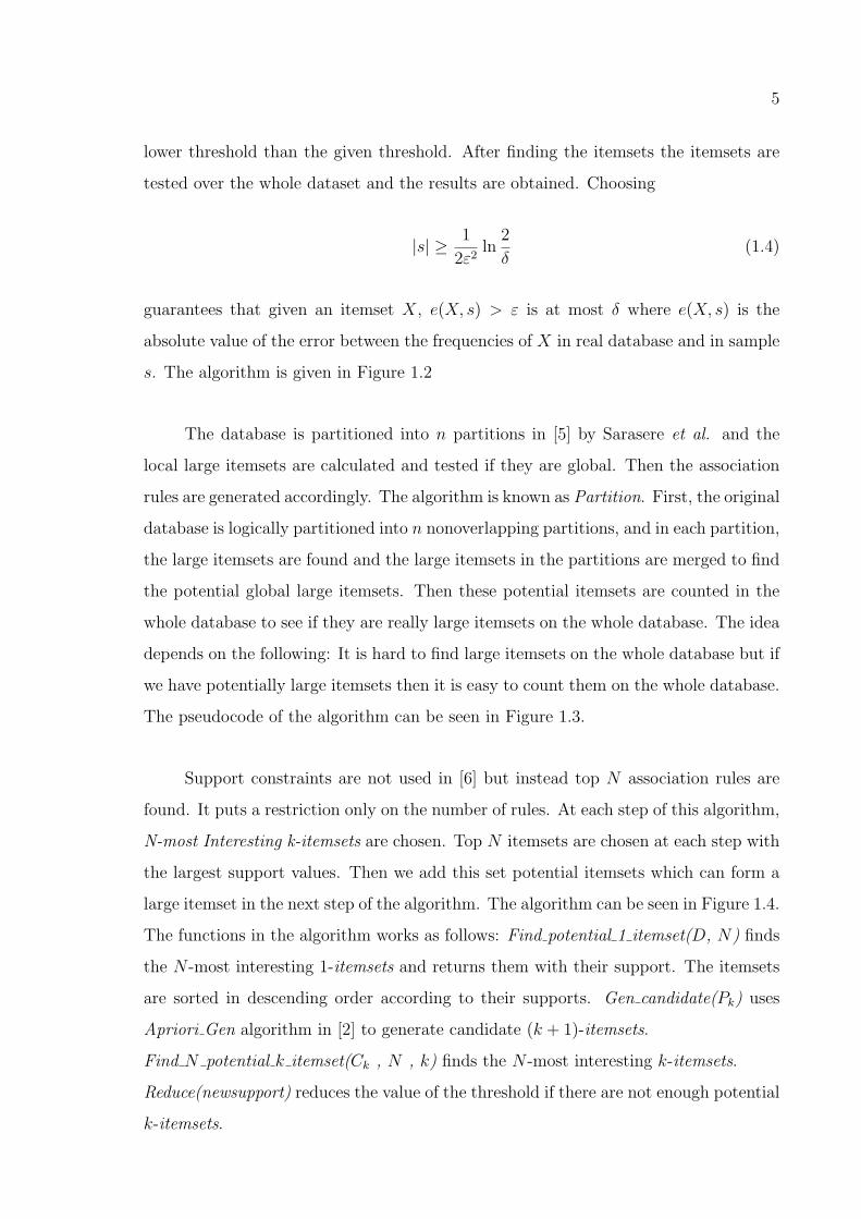
Toivonen [4] chooses a sample from the database which is smaller than the
database itself and calculates the rules in this sample. Then these rules are tested
on the whole database. The algorithm first chooses a random sample from the whole
database. Then the frequent itemsets are generated on this sample but with using
5
lower threshold than the given threshold. After finding the itemsets the itemsets are
tested over the whole dataset and the results are obtained. Choosing
|s| ≥ 1
2ε2ln
2
δ(1.4)
guarantees that given an itemset X, e(X, s) > ε is at most δ where e(X, s) is the
absolute value of the error between the frequencies of X in real database and in sample
s. The algorithm is given in Figure 1.2
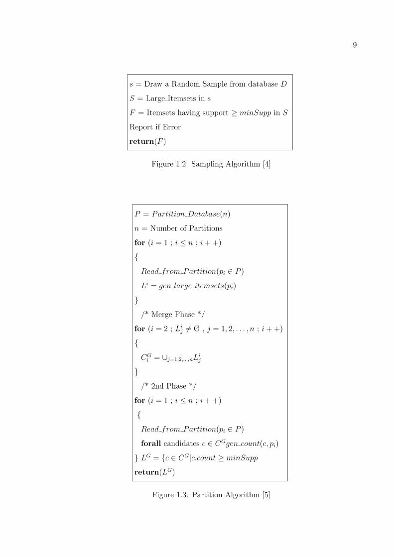
The database is partitioned into n partitions in [5] by Sarasere et al. and the
local large itemsets are calculated and tested if they are global. Then the association
rules are generated accordingly. The algorithm is known as Partition. First, the original
database is logically partitioned into n nonoverlapping partitions, and in each partition,
the large itemsets are found and the large itemsets in the partitions are merged to find
the potential global large itemsets. Then these potential itemsets are counted in the
whole database to see if they are really large itemsets on the whole database. The idea
depends on the following: It is hard to find large itemsets on the whole database but if
we have potentially large itemsets then it is easy to count them on the whole database.
The pseudocode of the algorithm can be seen in Figure 1.3.
Support constraints are not used in [6] but instead top N association rules are
found. It puts a restriction only on the number of rules. At each step of this algorithm,
N-most Interesting k-itemsets are chosen. Top N itemsets are chosen at each step with
the largest support values. Then we add this set potential itemsets which can form a
large itemset in the next step of the algorithm. The algorithm can be seen in Figure 1.4.
The functions in the algorithm works as follows: Find potential 1 itemset(D, N) finds
the N -most interesting 1-itemsets and returns them with their support. The itemsets
are sorted in descending order according to their supports. Gen candidate(Pk) uses
Apriori Gen algorithm in [2] to generate candidate (k + 1)-itemsets.
Find N potential k itemset(Ck , N , k) finds the N -most interesting k-itemsets.
Reduce(newsupport) reduces the value of the threshold if there are not enough potential
k-itemsets.

6
Hu, Chin and Takeichi [7] use functional languages for solving this problem. The
itemsets are stored in a list structure and the set of itemsets is a list of lists. The
threshold is specified not by giving a probability but giving a minimum number of
items that an itemset should contain.
Hipp et al. [8] use lattices and graphs for solving the problem of Association Rule
Mining.
Another way of mining association rules is to use distributed and parallel algo-
rithms. Suppose DB is a database with |D| transactions. Assume there are n sites.
Assume that the database is distributed into n parts DB1, DB2, . . . DBn. Let the size
of the partitions of DBi be Di, X.sup, X.supi be the global and local support counts
of an itemset X. An itemset is said to be globally large if X.sup ≥ s ×D for a given
support s. If X.supi ≥ s × Di then X is called globally large. L denotes the globally
large itemsets in DB. The task is to find L.
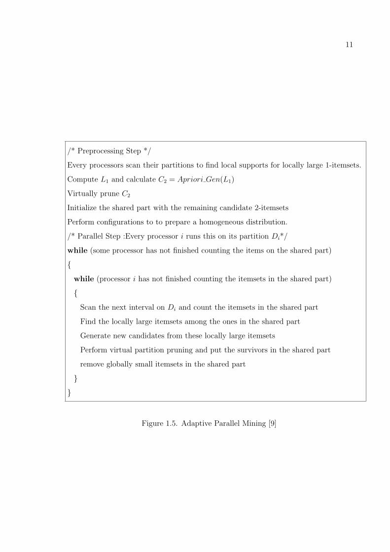
Adaptive Parallel Mining algorithm is implemented on a shared memory parallel
machine in [9] by David Cheung Kan. The algorithm is given in Figure 1.5.
Parallel algorithms for Mining Association Rules are defined in [10].
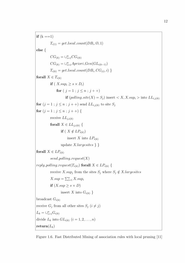
In [11] Cheung et al. implement a distributed algorithm for Mining Association
Rules. The algorithm is called FDM (Fast Distributed Mining of association rules).
The algorithm is given in Figure 1.6. The algorithm is iterated distributively at each
site Si until L(k) = Ø or the set of candidate sets CG(k) = Ø
Zaki [12] makes a survey on parallel and distributed mining of association rules.
Ganti et al. [13] focus on three basic problems of Data Mining. They define
and give references to various algorithms for solving problems of type market basket
analysis, clustering and classification.

7
In [14] Hipp et al. consider several Association Mining algorithms and compares
them.
1.2. Outline of Thesis
The rest of the thesis is organized as follows. In Section 2 we define the algo-
rithms used in the thesis. We give a detailed description of the algorithm Apriori and
we describe two statistical methods, Principal Component Analysis and k-Means Clus-
tering, to find correlations between sales of items. In Section 3 we give results obtained
using these methods and in the last chapter we conclude and discuss future work.

8
procedureLargeItemsets {let Large set L = Ø;
let Frontier set F = {Ø};while (F 6= Ø) {
let Candidate set C = Ø;
forall database tuples t {forall itemsets f in F {
if (t contains f) {let Cf = candidate itemsets that are extensions
of f and contained in t
forall itemsets cf in Cf {if(Cf ∈ C)
cf .count + +
else {cf .count = 0
C = C + cf
}}
}}
}let F = Ø
forall itemsets c in C {if count(c)/|D| > minsupp
L = L + c
if c should be used as a frontier in the next pass
F = F + c
}}
}
Figure 1.1. Finding large itemsets [1]
9
s = Draw a Random Sample from database D
S = Large Itemsets in s
F = Itemsets having support ≥ minSupp in S
Report if Error
return(F )
Figure 1.2. Sampling Algorithm [4]
P = Partition Database(n)
n = Number of Partitions
for (i = 1 ; i ≤ n ; i + +)
{Read from Partition(pi ∈ P )
Li = gen large itemsets(pi)
}/* Merge Phase */
for (i = 2 ; Lij 6= Ø , j = 1, 2, . . . , n ; i + +)
{CG
i = ∪j=1,2,...,nLij
}/* 2nd Phase */
for (i = 1 ; i ≤ n ; i + +)
{Read from Partition(pi ∈ P )
forall candidates c ∈ CGgen count(c, pi)
} LG = {c ∈ CG|c.count ≥ minSupp
return(LG)
Figure 1.3. Partition Algorithm [5]

10
Itemset Loop(supportk, lastsupportk, N, Ck, Pk, D) {(P1, support1, lassupport1) = find potential 1 itemset(D, N)
C2 = gen candidate(P1)
for(k= 2 ; k < m ; k++){(Pk, supportk, lastsupportk) = Find N potential k itemset(Ck, N, k)
if (k < m) Ck+1 = Gen Candidate(Pk) }Ik = N -most Interesting k-itemsets in Pk
I = ∪kIk
return(I)
}Find N potential k itemset(Ck, N, k) {
(Pk, supportk, lassupportk) = find potential k itemset(Ck, N)
newsupport = supportk
for (i = 2 ; i ≤ k ; i + +) updatedi = FALSE
for ( i = 2 ; i < m ; i + +){if (i== 1) {
if ( newsupport ≤ lastsupporti) {(Pi = find potential 1 itemsets with support(D,newsupport))
if (i < k) Ci+1 = gencandidate(Pi)
if (Ci+1 is updated)updatedi+1 = TRUE } }else {
if ((newsupport ≤ lastsupporti) || updatedi = TRUE) {(Pi = find potential k itemsets with support(Ci, newsupport))
if (i < k) Ci+1 = gencandidate(Pi)
if (Ci+1 is updated updatedi+1 = TRUE) } }if ( (number of k-items < N) && (i == k) && (k == m)) {
newsupport = reduce(newsupport)
for (j = 2 ; j ≤ k ; j + + updatedj = FALSE)
i = 1 } }return(Pk, supportk, lastsupportk)
}
Figure 1.4. Mining N most interesting itemsets [6]
11
/* Preprocessing Step */
Every processors scan their partitions to find local supports for locally large 1-itemsets.
Compute L1 and calculate C2 = Apriori Gen(L1)
Virtually prune C2
Initialize the shared part with the remaining candidate 2-itemsets
Perform configurations to to prepare a homogeneous distribution.
/* Parallel Step :Every processor i runs this on its partition Di*/
while (some processor has not finished counting the items on the shared part)
{while (processor i has not finished counting the itemsets in the shared part)
{Scan the next interval on Di and count the itemsets in the shared part
Find the locally large itemsets among the ones in the shared part
Generate new candidates from these locally large itemsets
Perform virtual partition pruning and put the survivors in the shared part
remove globally small itemsets in the shared part
}}
Figure 1.5. Adaptive Parallel Mining [9]
12
if (k ==1)
Ti(1) = get local count(DBi, Ø, 1)
else {CG(k) = ∪n
i=1CGi(k)
CG(k) = ∪ni=1Apriori Gen(GLi(k−1))
Ti(k) = get local count(DBi, CG(i), i) }forall X ∈ Ti(k)
if ( X.supi ≥ s×Di)
for ( j = 1 ; j ≤ n ; j + +)
if (polling site(X) = Sj) insert < X, X.supi > into LLi,j(k)
for (j = 1 ; j ≤ n ; j + +) send LLi,j(k) to site Sj
for (j = 1 ; j ≤ n ; j + +) {receive LLj,i(k)
forall X ∈ LLj,i(k) {if ( X /∈ LPi(k))
insert X into LPi(k)
update X.largesites } }forall X ∈ LPi(k)
send polling request(X)
reply polling request(Ti(k)) forall X ∈ LPi(k) {receive X.supj from the sites Sj where Sj /∈ X.largesites
X.sup =∑n
i=1 X.supi
if (X.sup ≥ s×D)
insert X into Gi(k) }broadcast Gi(k)
receive Gj from all other sites Sj (i 6= j)
Lk = ∪ni=1Gi(k)
divide Lk into GLi(k) (i = 1, 2, . . . , n)
return(Lk)
Figure 1.6. Fast Distributed Mining of association rules with local pruning [11]
13
2. METHODOLOGY
In our tests we used Apriori Algorithm for finding the association rules in the
input sets and we used Principal Component Analysis and k-Means algorithms for
clustering customers according to their buying habits.
2.1. Algorithm Apriori
2.1.1. Finding Large Itemsets
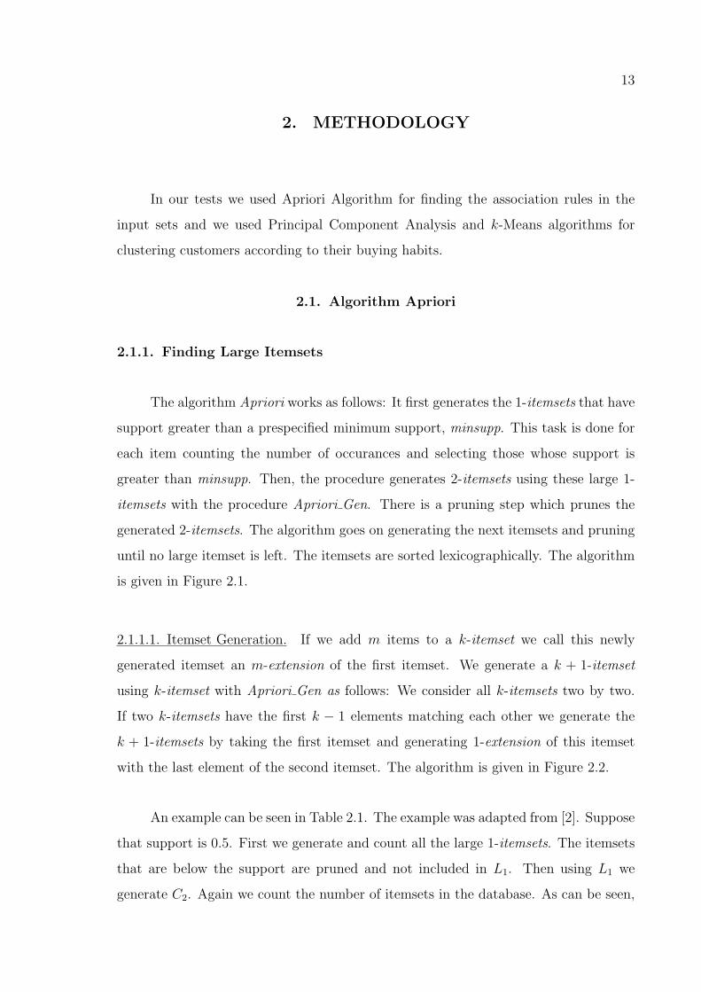
The algorithm Apriori works as follows: It first generates the 1-itemsets that have
support greater than a prespecified minimum support, minsupp. This task is done for
each item counting the number of occurances and selecting those whose support is
greater than minsupp. Then, the procedure generates 2-itemsets using these large 1-
itemsets with the procedure Apriori Gen. There is a pruning step which prunes the
generated 2-itemsets. The algorithm goes on generating the next itemsets and pruning
until no large itemset is left. The itemsets are sorted lexicographically. The algorithm
is given in Figure 2.1.
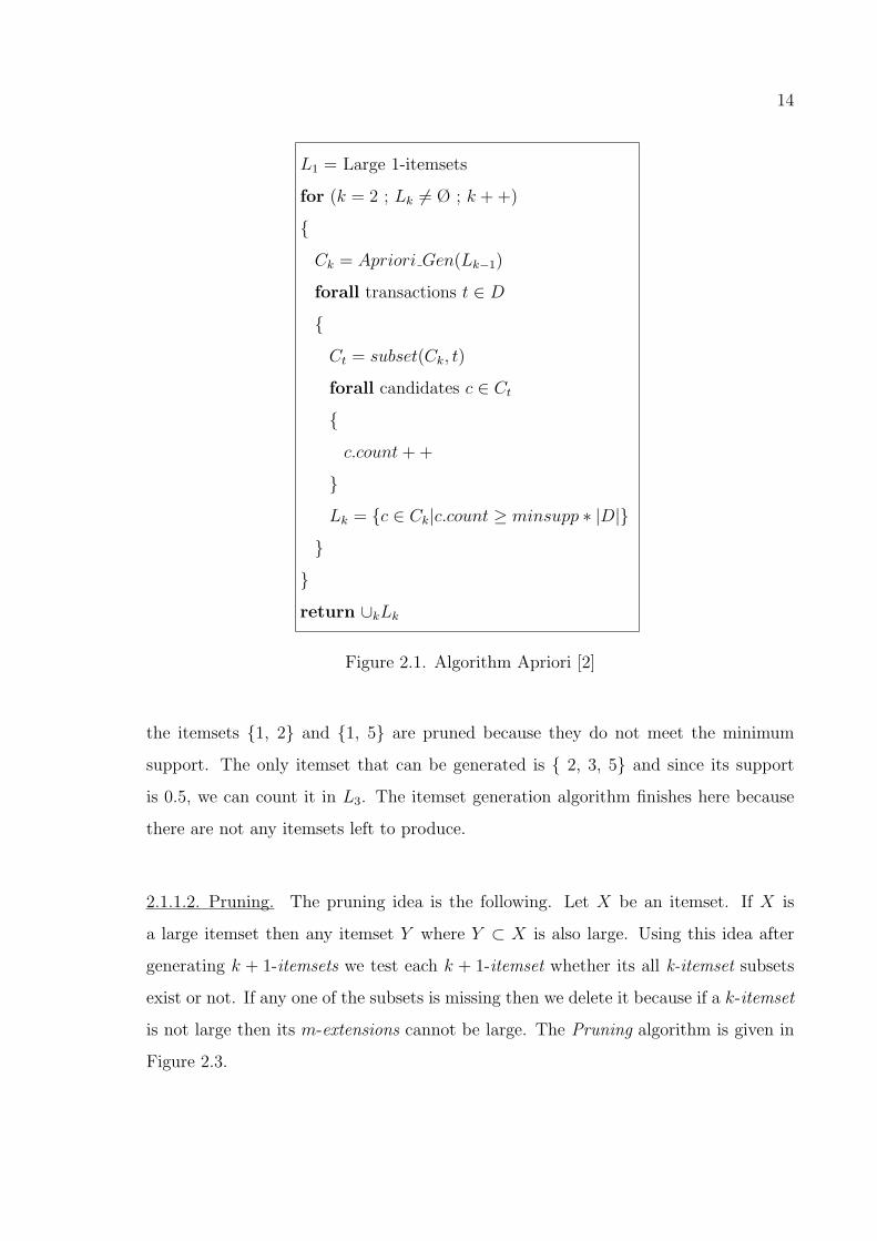
2.1.1.1. Itemset Generation. If we add m items to a k-itemset we call this newly
generated itemset an m-extension of the first itemset. We generate a k + 1-itemset
using k-itemset with Apriori Gen as follows: We consider all k-itemsets two by two.
If two k-itemsets have the first k − 1 elements matching each other we generate the
k + 1-itemsets by taking the first itemset and generating 1-extension of this itemset
with the last element of the second itemset. The algorithm is given in Figure 2.2.
An example can be seen in Table 2.1. The example was adapted from [2]. Suppose
that support is 0.5. First we generate and count all the large 1-itemsets. The itemsets
that are below the support are pruned and not included in L1. Then using L1 we
generate C2. Again we count the number of itemsets in the database. As can be seen,
14
L1 = Large 1-itemsets
for (k = 2 ; Lk 6= Ø ; k + +)
{Ck = Apriori Gen(Lk−1)
forall transactions t ∈ D
{Ct = subset(Ck, t)
forall candidates c ∈ Ct
{c.count + +
}Lk = {c ∈ Ck|c.count ≥ minsupp ∗ |D|}
}}return ∪kLk
Figure 2.1. Algorithm Apriori [2]
the itemsets {1, 2} and {1, 5} are pruned because they do not meet the minimum
support. The only itemset that can be generated is { 2, 3, 5} and since its support
is 0.5, we can count it in L3. The itemset generation algorithm finishes here because
there are not any itemsets left to produce.
2.1.1.2. Pruning. The pruning idea is the following. Let X be an itemset. If X is
a large itemset then any itemset Y where Y ⊂ X is also large. Using this idea after
generating k + 1-itemsets we test each k + 1-itemset whether its all k-itemset subsets
exist or not. If any one of the subsets is missing then we delete it because if a k-itemset
is not large then its m-extensions cannot be large. The Pruning algorithm is given in
Figure 2.3.

15
Table 2.1. Example of Apriori
D C1 L1
TID Items Itemset Support Itemset Support
100 1, 3, 4 1 0.5 1 0.5
200 2, 3, 5 2 0.75 2 0.75
300 1, 2, 3, 5 3 0.75 3 0.75
400 2, 5 4 0.25 5 0.75
5 0.75
C2 L2 C3
Itemset Support Itemset Support Itemset Support
1, 2 0.25 1, 3 0.5 2, 3, 5 0.5
1, 3 0.5 2, 3 0.5
1, 5 0.25 2, 5 0.75 L3
2, 3 0.5 3, 5 0.5 Itemset Support
2, 5 0.75 2, 3, 5 0.5
3, 5 0.5
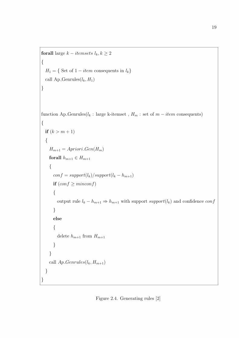
2.1.2. Generating Rules
2.1.2.1. Rule Generation. After all large itemsets have been generated they are used
to generate rules using minconf. In [2] there are two algorithms for this problem. In
our tests we used the following algorithm.
We know that if a ⇒ (l − a) does not hold then a ⇒ (l − a) cannot hold where
a ⊂ a (If a smaller set is not large then its m-extensions cannot be large). Suppose
X = {ABC} and Y = {D}. If the rule {ABC} ⇒ {D} does not hold then the rule
{AB} ⇒ {CD} cannot hold because its confidence is always smaller than the first one.
Rewriting this as for (l − r) ⇒ r to hold all rules of the form (l − r) ⇒ r must hold
where r ⊂ r and r 6= Ø. Returning to the above example for the rule {AB} ⇒ {CD}
16
forall p, q ∈ Lk
{if (p.item1 = q.item1, p.item2 = q.item2 . . . p.itemk−1 = q.itemk−1)
{insert into Ck+1{p.item1, p.item2, . . . , p.itemk, q.itemk}
}}
Figure 2.2. Candidate generation [2]
to hold the two rules {ABC} ⇒ {D} and {ABD} ⇒ {C} must hold. The algorithm in
Figure 2.4 uses this idea [2]. Coming back to our example in Table 2.1, let us generate
the rules for confidence = 1.0. Generation of rules from large 2-itemsets is trivial. For
each itemset we put one of the items in the consequent and we calculate the rules. So
we have 1 ⇒ 3, 2 ⇒ 3, 2 ⇒ 5, 5 ⇒ 2, 5 ⇒ 3. The other rules do not have confidence
equal to 1.0. For generating rules with 3-itemsets we first find the 1-item consequents
in the itemset. For example let us consider the itemset s = {2, 3, 5}. First we generate
all 1-items in s. We have {2}, {3} and {5}. Then we use the Apriori Gen function
to generate 2-itemsets from these three items. Now we have {2, 3} {2, 5} and {3, 5}.Then for each of these we test: support({2, 3, 5})/support({2, 3}) = 1.0 so we generate
the rule 2, 3 ⇒ 5. Then we test support({2, 3, 5})/support({3, 5}) = 1.0 so we generate
the rule 3, 5 ⇒ 2. We then test support({2, 3, 5})/support({2, 5}) < 1.0 so we do not
consider it in the second phase.
2.2. Principal Component Analysis
If we look at the transactions by each customer, then we can represent each
customer with t with a n-dimensional vector xt where xti represents the amount of item
i bought by customer t. The n items are chosen as the n items sold most. By looking at
the correlations between xi over all customers, we find all dependencies between items.
The method we use is called Principal Component Analysis (PCA) [15]. Suppose we
have a dataset which consists of items that have n attributes. We are looking for a set

17
forall itemsets c ∈ Ck
{forall (k − 1) subsets s of c
{if (s /∈ Lk−1)
{delete c from Ck
}}
}
Figure 2.3. Pruning [2]
of d orthogonal directions which best explains the data. Thus what we want is a linear
transformation of the form
zi = A(xi − x) (2.1)
such that E[x] = x and Cov(x) = S. We have E[z] = 0 and Cov(z) = D where D is a
diagonal matrix. This means after the transformation zi are zero mean and correlations
are eliminated. We have if z = Ax then Cov(z) = ASA′ and we require Cov(z) to be a
diagonal matrix. So if we take a1, a2, . . . , an as eigenvectors of S then new dimensions
z1, z2, . . . , zd can be defined as
zi = a′ix (2.2)
having Var(zi) = λi. We can use the largest of the eigenvalues discarding the rest. The
amount of variance explained by the eigenvectors can be found by
λ1 + λ2 + · · ·+ λd
λ1 + λ2 + · · ·+ λn
(2.3)
18
If the first few dimensions can explain the variance upto a percentage threshold that can
be tolerated then we can discard the rest. If we can reduce the number of dimensions
to two we can then plot the data. Because in our application, xi have different units;
grams, pieces, etc, we work with the correlation matrix R rather than the covariance
matrix S.
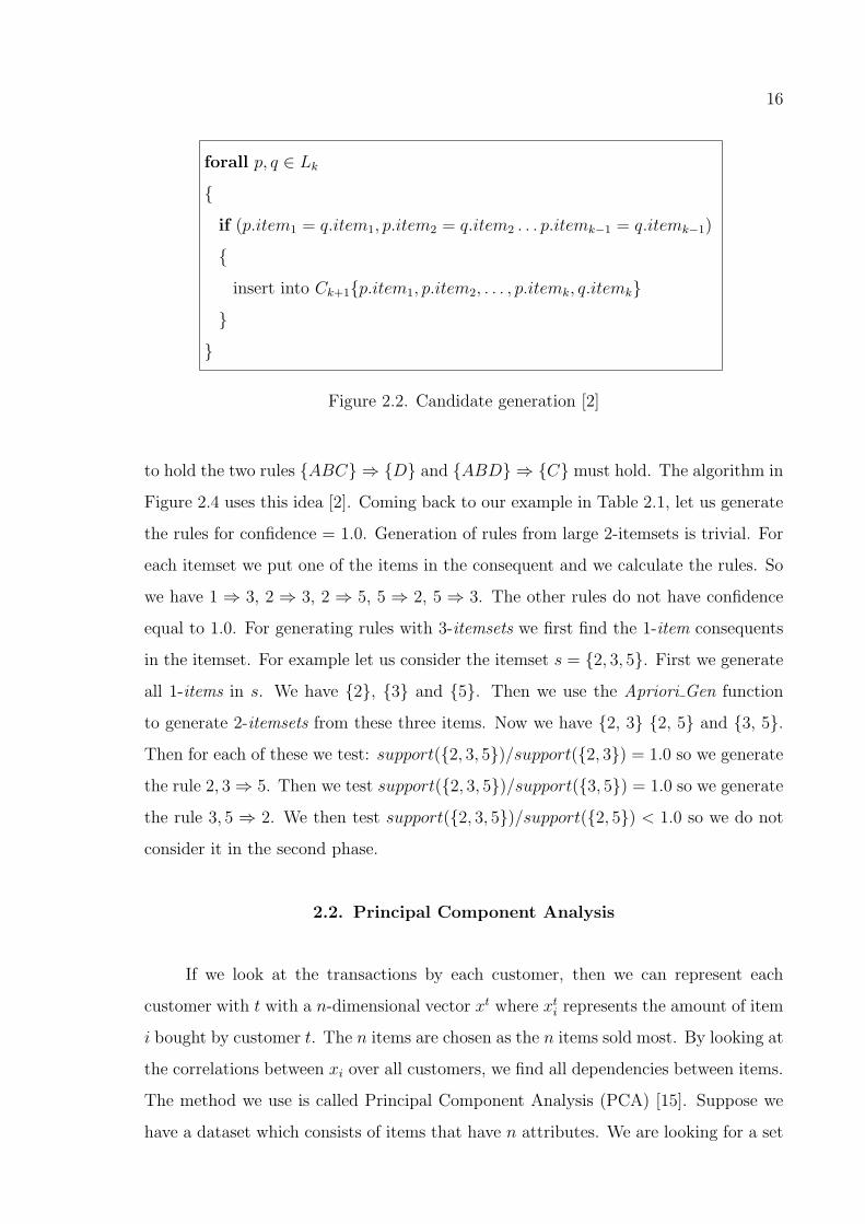
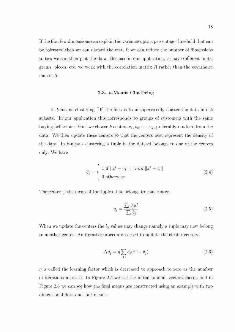
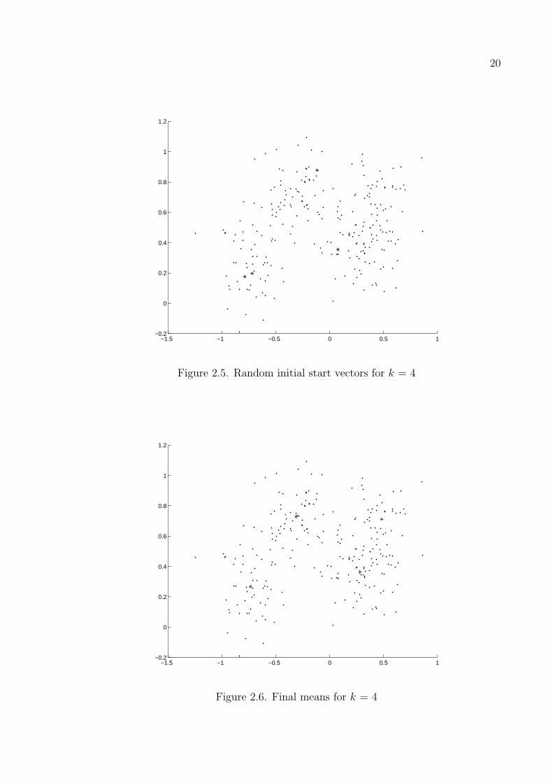
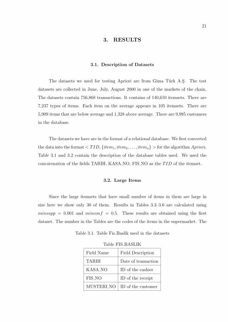
2.3. k-Means Clustering
In k-means clustering [16] the idea is to unsupervisedly cluster the data into k
subsets. In our application this corresponds to groups of customers with the same
buying behaviour. First we choose k centers v1, v2, . . . , vk, preferably random, from the
data. We then update these centers so that the centers best represent the density of
the data. In k-means clustering a tuple in the dataset belongs to one of the centers
only. We have
btj =
1 if ||xt − vj|| = minl||xt − vl||0 otherwise
(2.4)
The center is the mean of the tuples that belongs to that center.
vj =
∑t b
tjx
t
∑t b
tj
(2.5)
When we update the centers the bj values may change namely a tuple may now belong
to another center. An iterative procedure is used to update the cluster centers.
∆vj = η∑
t
btj(x
t − vj) (2.6)
η is called the learning factor which is decreased to approach to zero as the number
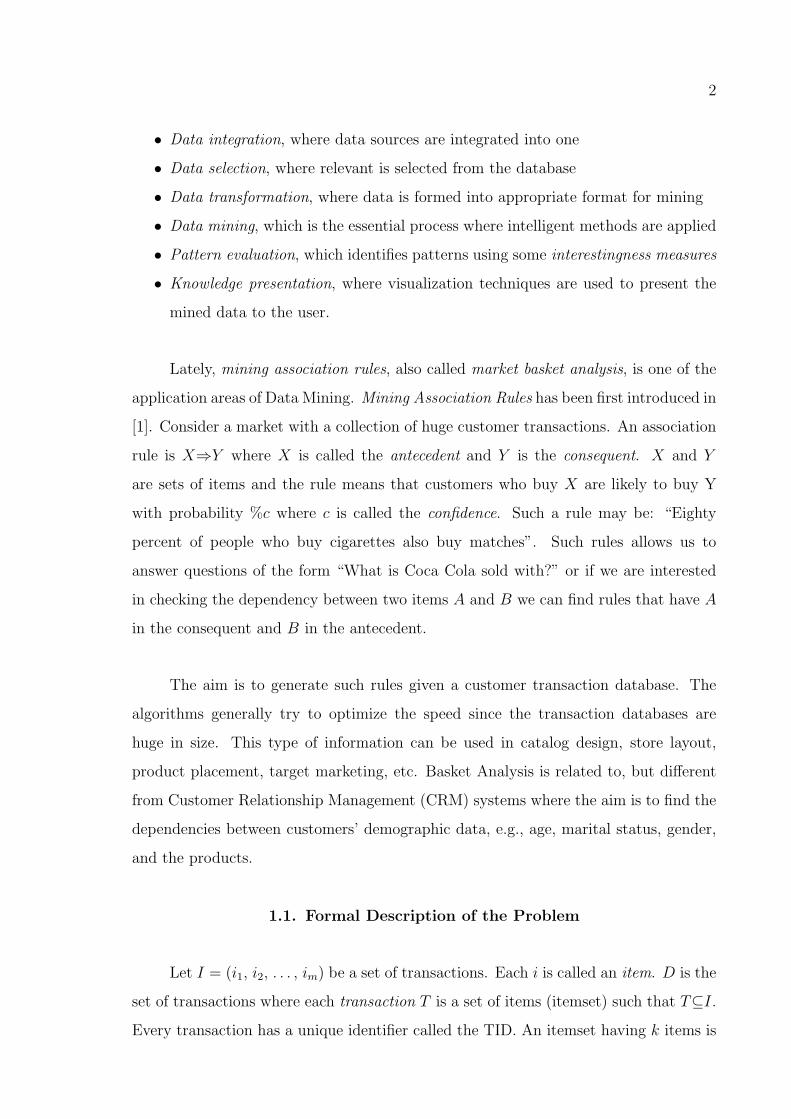
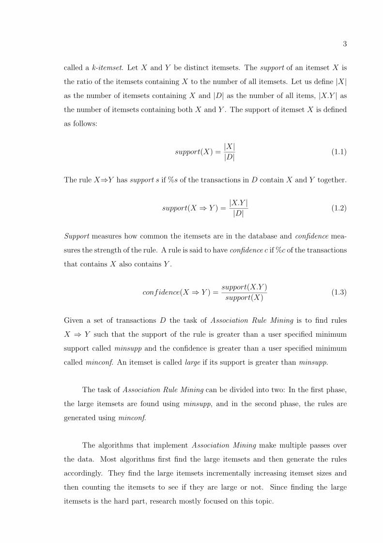
of iterations increase. In Figure 2.5 we see the initial random vectors chosen and in
Figure 2.6 we can see how the final means are constructed using an example with two
dimensional data and four means.
19
forall large k − itemsets lk, k ≥ 2
{H1 = { Set of 1− item consequents in lk}call Ap Genrules(lk, H1)
}
function Ap Genrules(lk : large k-itemset , Hm : set of m− item consequents)
{if (k > m + 1)
{Hm+1 = Apriori Gen(Hm)
forall hm+1 ∈ Hm+1
{conf = support(lk)/support(lk − hm+1)
if (conf ≥ minconf)
{output rule lk − hm+1 ⇒ hm+1 with support support(lk) and confidence conf
}else
{delete hm+1 from Hm+1
}}call Ap Genrules(lk, Hm+1)
}}
Figure 2.4. Generating rules [2]
20
−1.5 −1 −0.5 0 0.5 1−0.2
0
0.2
0.4
0.6
0.8
1
1.2
Figure 2.5. Random initial start vectors for k = 4
−1.5 −1 −0.5 0 0.5 1−0.2
0
0.2
0.4
0.6
0.8
1
1.2
Figure 2.6. Final means for k = 4
21
3. RESULTS
3.1. Description of Datasets
The datasets we used for testing Apriori are from Gima Turk A.S. The test
datasets are collected in June, July, August 2000 in one of the markets of the chain.
The datasets contain 756,868 transactions. It contains of 140,610 itemsets. There are
7,237 types of items. Each item on the average appears in 105 itemsets. There are
5,909 items that are below average and 1,328 above average. There are 9,985 customers
in the database.
The datasets we have are in the format of a relational database. We first converted
the data into the format < TID, {item1, item2, . . . , itemn} > for the algorithm Apriori.
Table 3.1 and 3.2 contain the description of the database tables used. We used the
concatenation of the fields TARIH, KASA NO, FIS NO as the TID of the itemset.
3.2. Large Items
Since the large itemsets that have small number of items in them are large in
size here we show only 30 of them. Results in Tables 3.3–3.6 are calculated using
minsupp = 0.001 and minconf = 0.5. These results are obtained using the first
dataset. The number in the Tables are the codes of the items in the supermarket. The
Table 3.1. Table Fis Baslik used in the datasets
Table FIS BASLIK
Field Name Field Description
TARIH Date of transaction
KASA NO ID of the cashier
FIS NO ID of the receipt
MUSTERI NO ID of the customer

22
Table 3.2. Table Fis Detay used in the datasets
Table FIS DETAY
Field Name Field Description
TARIH Date of transaction
KASA NO ID of the cashier
FIS NO ID of the receipt
FIS SIRANO The place of the item in that receipt
MAL NO ID of the item
MIKTAR The amount of the item
data is confidential so it may not be used without the permission from the owner. We
give some meaningful examples of real life results in the next section.
3.3. Rules Generated
According to the large itemsets in Tables 3.3–3.6, using minconf, the rules in
Tables 3.7–3.9 are generated.
3.4. Finding Correlations Using PCA
There are twelve datasets from twelve stores of the chain. For each of the stores
we found the items that are sold the most and the customers that have bought the
most number of items (We chose 1000 customers from each store). Then we merged the
stores for new items and customers. We wanted to reduce the number of dimensions
on items to see if we could cluster the customers with two dimensions on items. The
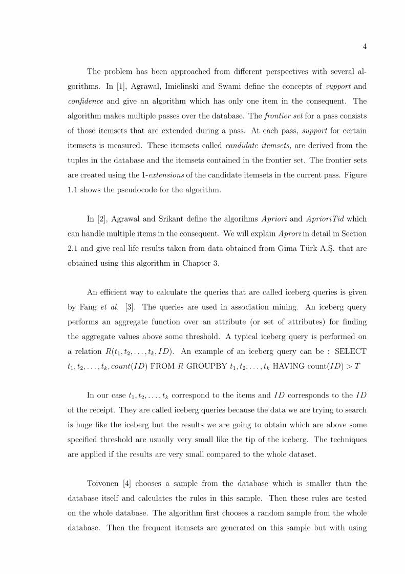
results in Figure 3.1 are obtained by taking the number of items as 25 on store 102. The
Table 3.10 shows how much of the variances are explained using the specified number
of dimensions. Energy denotes the percentage of variance explained of the original
data reducing the number of dimensions to that number. The data in the graphics are
sorted lexicogaphically. Similar results using different datasets and different number of
dimensions can be seen in Appendix A.
23
Table 3.3. Large 1-itemsets
Item1 Support
4309020094 0.147998
9917010003 0.080164
9917010001 0.077057
4309020010 0.076054
4308020094 0.072918
4309020001 0.045203
4308020019 0.043553
5808010069 0.043503
4308020071 0.040366
4308020052 0.040359
4309020083 0.039321
4909020002 0.037557
4309020076 0.036995
4309020075 0.034563
4308020080 0.032799
4309020012 0.030837
4909020090 0.028340
4909010007 0.025823
4309020008 0.024564
4309020078 0.024080
4309020013 0.023924
4308020089 0.023895
4309020014 0.023853
4309020098 0.023476
4308020098 0.023070
4309020016 0.022366
4309020095 0.022245
5101010005 0.020667
4308020070 0.020638
5308020087 0.020624

24
Table 3.4. Large 2-itemsets
Item1 Item2 Support
4309020010 4309020094 0.051255
4308020094 4309020094 0.028952
4309020001 4309020094 0.021599
4309020012 4309020094 0.020546
4309020094 9917010001 0.019913
4309020076 4309020094 0.019166
4309020083 4309020094 0.017723
4308020094 4309020010 0.017559
4308020052 4309020094 0.017396
4309020075 4309020094 0.017040
4309020094 9917010003 0.015419
4309020014 4309020094 0.014615
4309020094 5808010069 0.014501
4309020001 4309020010 0.013029
4309020013 4309020094 0.012624
4308020019 4309020094 0.012417
4308020080 4309020094 0.012396
4309020016 4309020094 0.012261
9917010001 9917010003 0.012140
4309020001 4309020008 0.011678
4308020071 4309020094 0.011550
4308020052 4309020010 0.011436
4309020094 4309020098 0.011329
4309020010 4309020083 0.011329
4308020080 4308020094 0.010924
4309020008 4309020094 0.010774
4309020010 4309020076 0.010760
4309020010 4309020012 0.010689
4309020078 4309020094 0.010412
4308020019 4308020094 0.010149
25
Table 3.5. Large 3-itemsets
Item1 Item2 Item3 Support
4308020094 4309020010 4309020094 0.012368
4309020001 4309020010 4309020094 0.009885
4309020010 4309020012 4309020094 0.008712
4308020052 4309020010 4309020094 0.008506
4309020010 4309020083 4309020094 0.008193
4309020010 4309020076 4309020094 0.007958
4309020010 4309020075 4309020094 0.007460
4309020010 4309020094 9917010001 0.006756
4309020010 4309020014 4309020094 0.006379
4309020001 4309020008 4309020094 0.006024
4309020010 4309020094 5808010069 0.005839
4309020075 4309020076 4309020094 0.005725
4308020094 4309020001 4309020094 0.005597
4309020010 4309020094 9917010003 0.005547
4308020080 4309020010 4309020094 0.005398
4309020001 4309020076 4309020094 0.005355
4308020094 4309020076 4309020094 0.005291
4308020071 4309020010 4309020094 0.005249
4308020052 4308020094 4309020094 0.005199
4309020010 4309020016 4309020094 0.005156
4309020010 4309020013 4309020094 0.005028
4308020094 4309020075 4309020094 0.004993
4308020019 4309020010 4309020094 0.004971
4308020080 4308020094 4309020094 0.004943
4308020094 4309020083 4309020094 0.004850
4309020001 4309020075 4309020094 0.004793
4308020052 4309020001 4309020094 0.004765
4309020010 4309020094 4309020098 0.004751
4309020008 4309020010 4309020094 0.004694
4309020010 4309020078 4309020094 0.004644
26
Table 3.6. Large 4-itemsets
Item1 Item2 Item3 Item4 Support
4308020094 4309020001 4309020010 4309020094 0.002937
4309020010 4309020075 4309020076 4309020094 0.002895
4309020001 4309020008 4309020010 4309020094 0.002880
4308020052 4309020001 4309020010 4309020094 0.002795
4308020052 4308020094 4309020010 4309020094 0.002795
4309020001 4309020010 4309020076 4309020094 0.002752
4309020001 4309020010 4309020012 4309020094 0.002731
4308020094 4309020010 4309020076 4309020094 0.002710
4308020094 4309020010 4309020075 4309020094 0.002624
4308020094 4309020010 4309020083 4309020094 0.002574
4309020001 4309020010 4309020075 4309020094 0.002539
4308020080 4308020094 4309020010 4309020094 0.002525
4308020052 4309020010 4309020083 4309020094 0.002382
4309020001 4309020010 4309020083 4309020094 0.002240
4309020001 4309020008 4309020075 4309020094 0.002240
4308020089 4308020094 4309020010 4309020094 0.002155
4308020019 4308020094 4309020010 4309020094 0.002141
4309020010 4309020012 4309020076 4309020094 0.002070
4308020052 4309020010 4309020076 4309020094 0.002020
4309020001 4309020075 4309020076 4309020094 0.002006
4309020010 4309020075 4309020083 4309020094 0.001991
4309020010 4309020014 4309020076 4309020094 0.001977
4309020010 4309020013 4309020075 4309020094 0.001977
4308020094 4309020010 4309020012 4309020094 0.001977
4309020008 4309020010 4309020075 4309020094 0.001949
4308020094 4309020010 4309020014 4309020094 0.001949
4309020001 4309020010 4309020014 4309020094 0.001878
4309020001 4309020010 4309020013 4309020094 0.001870
4309020010 4309020076 4309020083 4309020094 0.001856
4308020094 4309020010 4309020016 4309020094 0.001856
27
Table 3.7. Rules generated using large 2-itemsets
Confidence Support
4309020010 ⇒ 4309020094 0.673929 0.051255
4309020012 ⇒ 4309020094 0.666282 0.020546
4309020076 ⇒ 4309020094 0.518069 0.019166
4309020014 ⇒ 4309020094 0.612701 0.014614
4309020013 ⇒ 4309020094 0.527645 0.012623
4309020016 ⇒ 4309020094 0.548171 0.012260
3.5. Clustering Customers Using k-Means
Among the twelve stores we found the items that are sold the most in all the
stores. We chose 25, 46, 100 items and we ran k-Means algorithm on them. We wanted
to group the customers according to their buying habits. We clustered the customers in
4, 8, 12, 16, 20 groups and from these we tried to guess what the customers buy belong-
ing to that cluster. The results in Table 3.11 are taken from the store 102 with choosing
the number of items 25 and number of clusters as 4. The numbers above the means
show the percentage of the customers belonging to that cluster. We first normalized
the data acording to the items to disable the effect of difference variances and means
in the data. Similar results with different datasets and different means can be seen in
Appendix B. For example if we look at Table 3.11 we can say the people in this group
buy the items ’4101020081’, ’4101040001’, ’4102010002’, ’4102020001’, ’4103030095’,
’4104020082’, ’4109010096’, ’4109010100’, ’4109010100’, ’4109010177’ more than other
customers. Such results can be derived for other stores and items.

28
Table 3.8. Rules generated using large 3-itemsets
Confidence Support
4308020094 4309020010 ⇒ 4309020094 0.704333 0.012367
4309020001 4309020010 ⇒ 4309020094 0.758733 0.009885
4309020010 4309020012 ⇒ 4309020094 0.815036 0.008712
4308020052 4309020010 ⇒ 4309020094 0.743781 0.008505
4309020010 4309020083 ⇒ 4309020094 0.723163 0.008192
4309020010 4309020076 ⇒ 4309020094 0.739590 0.007958
4309020010 4309020075 ⇒ 4309020094 0.747150 0.007460
4309020010 9917010001 ⇒ 4309020094 0.779967 0.006756
4309020010 4309020014 ⇒ 4309020094 0.770618 0.006379
4309020008 4309020094 ⇒ 4309020001 0.559075 0.006023
4309020001 4309020008 ⇒ 4309020094 0.515834 0.006023
4309020010 5808010069 ⇒ 4309020094 0.740974 0.005838
4309020075 4309020076 ⇒ 4309020094 0.594534 0.005725
4308020094 4309020001 ⇒ 4309020094 0.641401 0.005597
4309020010 9917010003 ⇒ 4309020094 0.737240 0.005547
4308020080 4309020010 ⇒ 4309020094 0.726315 0.005397
4309020001 4309020076 ⇒ 4309020094 0.643040 0.005355
4308020094 4309020076 ⇒ 4309020094 0.619483 0.005291
4308020071 4309020010 ⇒ 4309020094 0.746208 0.005248
4308020052 4308020094 ⇒ 4309020094 0.581081 0.005198
4309020010 4309020016 ⇒ 4309020094 0.782937 0.005156
4309020010 4309020013 ⇒ 4309020094 0.793490 0.005028
4308020094 4309020075 ⇒ 4309020094 0.617957 0.004992
4308020019 4309020010 ⇒ 4309020094 0.680623 0.004971
4308020094 4309020083 ⇒ 4309020094 0.603539 0.004850
4309020001 4309020075 ⇒ 4309020094 0.601785 0.004793
4308020052 4309020001 ⇒ 4309020094 0.638095 0.004764
4309020010 4309020098 ⇒ 4309020094 0.820638 0.004750
4309020008 4309020010 ⇒ 4309020094 0.718954 0.004693
4309020010 4309020078 ⇒ 4309020094 0.702906 0.004644
29
Table 3.9. Rules generated using large 4-itemsets
Confidence Support
4308020094 4309020001 4309020094 ⇒ 4309020010 0.524777 0.002937
4308020094 4309020001 4309020010 ⇒ 4309020094 0.783681 0.002937
4309020075 4309020076 4309020094 ⇒ 4309020010 0.505590 0.002894
4309020010 4309020075 4309020076 ⇒ 4309020094 0.785714 0.002894
4309020008 4309020010 4309020094 ⇒ 4309020001 0.613636 0.002880
4309020001 4309020008 4309020010 ⇒ 4309020094 0.758426 0.002880
4308020052 4308020094 4309020094 ⇒ 4309020010 0.537619 0.002794
4308020052 4308020094 4309020010 ⇒ 4309020094 0.770588 0.002794
4308020052 4309020001 4309020094 ⇒ 4309020010 0.586567 0.002794
4308020052 4309020001 4309020010 ⇒ 4309020094 0.806981 0.002794
4309020001 4309020076 4309020094 ⇒ 4309020010 0.513944 0.002752
4309020001 4309020010 4309020076 ⇒ 4309020094 0.804573 0.002752
4309020001 4309020012 4309020094 ⇒ 4309020010 0.592592 0.002730
4309020001 4309020010 4309020012 ⇒ 4309020094 0.860986 0.002730
4308020094 4309020076 4309020094 ⇒ 4309020010 0.512096 0.002709
4308020094 4309020010 4309020076 ⇒ 4309020094 0.765060 0.002709
4308020094 4309020075 4309020094 ⇒ 4309020010 0.525641 0.002624
4308020094 4309020010 4309020075 ⇒ 4309020094 0.771966 0.002624
4308020094 4309020083 4309020094 ⇒ 4309020010 0.530791 0.002574
4308020094 4309020010 4309020083 ⇒ 4309020094 0.763713 0.002574
4309020001 4309020075 4309020094 ⇒ 4309020010 0.529673 0.002538
4309020001 4309020010 4309020075 ⇒ 4309020094 0.805869 0.002538
4308020080 4308020094 4309020094 ⇒ 4309020010 0.510791 0.002524
4308020080 4308020094 4309020010 ⇒ 4309020094 0.748945 0.002524
4308020052 4309020083 4309020094 ⇒ 4309020010 0.563025 0.002382
4308020052 4309020010 4309020083 ⇒ 4309020094 0.801435 0.002382
4309020008 4309020075 4309020094 ⇒ 4309020001 0.552631 0.002240
4309020001 4309020008 4309020075 ⇒ 4309020094 0.621301 0.002240
4309020001 4309020083 4309020094 ⇒ 4309020010 0.535714 0.002240
4309020001 4309020010 4309020083 ⇒ 4309020094 0.775862 0.002240

30
Table 3.10. Energies in 25 dimensions
Dimensions Energy 102 Energy 221 Energy 310 Energy All
1 8.7208 6.9129 10.1739 8.1142
2 15.6119 12.7856 16.1699 13.7807
3 20.8453 18.5378 21.4567 19.0488
4 25.9380 23.6384 26.5827 23.7955
5 30.6403 28.6230 31.2361 28.2390
6 35.0867 33.5463 35.8104 32.4682
7 39.4677 38.1337 40.2429 36.6690
8 43.8048 42.5995 44.5389 40.7784
9 47.8813 47.0094 48.7484 44.8294
10 51.9463 51.1029 52.8931 48.7786
11 55.9833 55.1006 56.8524 52.6275
12 59.9066 58.8579 60.7106 56.4191
13 63.7028 62.5834 64.5277 60.1386
14 67.3764 66.2440 68.0754 63.8380
15 70.9363 69.7447 71.5919 67.5117
16 74.4453 73.2220 75.0060 71.1116
17 77.8364 76.6103 78.3337 74.6617
18 81.1350 79.8747 81.5901 78.1426
19 84.3484 82.9969 84.7261 81.5400
20 87.2908 86.0823 87.8119 84.8643
21 90.1221 89.0275 90.8644 88.0972
22 92.7572 91.9632 93.8624 91.2881
23 95.3390 94.8034 96.4892 94.4452
24 97.7911 97.4242 98.3662 97.3642
25 100.0000 100.0000 100.0000 100.0000
31
Table 3.11. Store 102 with 4 means
4-MEANS
ITEMS 14.5% 7.7% 74.2% 3.6%
0809010004 -0.0032 0.0708 -0.0021 -0.0943
4101020081 0.7886 0.0955 -0.1680 0.0818
4101040001 0.9433 -0.0560 -0.1809 0.0490
4102010002 0.7653 -0.2170 -0.1311 0.0829
4102020001 0.4336 0.1444 -0.1258 0.5366
4103030095 1.0121 -0.0917 -0.1948 0.1351
4104020082 1.2247 -0.1571 -0.2115 -0.2366
4104020088 -0.1241 0.0859 -0.0583 1.5189
4107020002 0.1045 0.2944 -0.0822 0.6440
4109010005 -0.0826 1.7914 -0.1796 0.2035
4109010022 -0.1053 -0.0933 -0.1489 3.6935
4109010032 -0.0298 0.1768 -0.0162 0.0765
4109010036 0.0761 0.0463 -0.0189 -0.0155
4109010047 -0.1351 1.5145 -0.1443 0.2790
4109010048 0.1592 0.2156 -0.1066 1.0938
4109010082 -0.0301 0.2896 -0.0190 -0.1065
4109010096 0.8351 -0.0977 -0.1425 -0.2171
4109010100 0.5603 0.2499 -0.1385 0.0636
4109010103 -0.0804 0.1851 -0.0698 1.3661
4109010114 0.4763 0.1087 -0.1131 0.1804
4109010115 -0.0377 -0.1005 0.0130 0.0999
4109010177 1.0103 -0.1649 -0.1723 -0.1652
4109010178 0.2307 0.2406 -0.0675 -0.0523
4109010179 -0.0408 1.1408 -0.1069 -0.0730
4110040081 -0.0927 1.0201 -0.1077 0.4110

32
0 10 20 30 40 50 60 70 80 90 1000
10
20
30
40
50
60
70
80
90
100
Number of attributes
Per
cent
age
expl
aine
dEnergy in 102
−15 −10 −5 0 5 10 150
5
10
15
20
25
Data 102
X2
X1
Figure 3.1. Energy and data reduced to 2 dimensions for 25 items for store number
102

33
4. CONCLUSIONS AND FUTURE WORK
Apriori Algorithm [2] is one of the fastest and earliest tools for Association Min-
ing. We used the apriori algorithm for mining Association Rules in the large database
of Gima Turk A.S. The data used in the thesis was confidential so we mined data
blindly i.e. not knowing what we mined. As seen in the results in the previous section
what we knew about the data is the ID’s of the items. We tried to cluster the customers
according to their buying habits according to these items. Our first data set was taken
in summer and we had the following results. The item which is sold the most came out
to be tomato. Tomato was present in 14 per cent of the transactions. The second most
sold item was bread which is not surprising for our country, then came the cucumbers.
The top remaining items also turned out to be items that are mostly used in making
salads and Coke. As a result we can conclude that our people eat salad very much in
summer time. Let me give examples of rules derived from these large itemsets. The
people who bought cucumbers also bought tomato with confidence 67 per cent. By
saying 67 per cent confidence we mean that 67 per cent of people who bought cucum-
bers also bought tomatoes. Note that we do not have a rule saying that 67 per cent
of people who bought tomatoes also bought cucumbers because although the itemset
{tomato, cucumber} is large the confidence of the rule tomato ⇒ cucumber does not
have enough confidence. Another such rule may be 66 per cent of people who bought
green pepper also bought tomatoes. If we give examples of rules with three items we
have 55per cent of people who bought dill and tomato also bought parsley.
We tried to cluster the customers and items using PCA. We wanted to reduce
dimensions to two and to see the plotted data. Since the variances in the data were
near each other reducing the number of dimensions to two did not cluster the data.
We then used k-Means clustering with k = 4, 8, 12, 16, 20 to cluster the data.
Since the data was confidential we did not have the chance to make comments
on the data. We only could blindly mine and find association rules. If we had more
knowledge on the data then we could derive more results. The data consisted of items

34
and the amount of items sold at each transaction. Since we did not know what the
item was the amount did not mean anything to us. Also some of the amounts were in
fractions i.e in kilogram and some of them were in numbers so we did not have a way
of using the amount of the item in the mining of the data. We had to take the data as
binary i.e. it exists in this transaction or not. Also since the data was confidential we
did not have information on the prices of the items to prioritize the items. A future
work could be to use the information in the amount of the items and their prices for
deriving more meaningful rules.
The dataset we used did not contain the hierarchical information about the items.
This means we have wine of brand X, wine of brand Y as different itemsets and the
ID’s of these items do not have a hierarchy saying that these items are Wines. If
the data is supplied with hierarchical information then we can find relations such as
“People who buy Wines also buy Cheese” but now we can only derive rules such as
“People who buy Wine brand X also buy Cheese of brand Z.”
We implemented the apriori algorithm which is one of the first and fastest meth-
ods. Most of the methods for Mining Association Rules depend on this algorithm. We
implemented a sequential algorithm but there are parallel and distributed algorithms
for this problem which can be implemented for speeding up computations as a future
work.
35
APPENDIX A: RESULTS OF PRINCIPAL COMPONENT
ANALYSIS
The results in Figures A.1–A.3 are obtained by taking the number of items as
25 on stores with numbers 221, 310 and the whole dataset respectively. The results
in Figures A.4–A.7 are obtained by taking the number of items as 46 on stores with
numbers 102, 221, 310 and the whole dataset respectively. The results in Figures
A.8–A.11 are obtained by taking the number of items as 100 on stores with numbers
102, 221, 310 and the whole dataset respectively. The Tables A.1–A.2 shows how
much of the variances are explained using the specified number of dimensions. Energy
denotes the percentage of variance explained of the original data reducing the number
of dimensions to that number. The data in the graphics are sorted lexicogaphically.
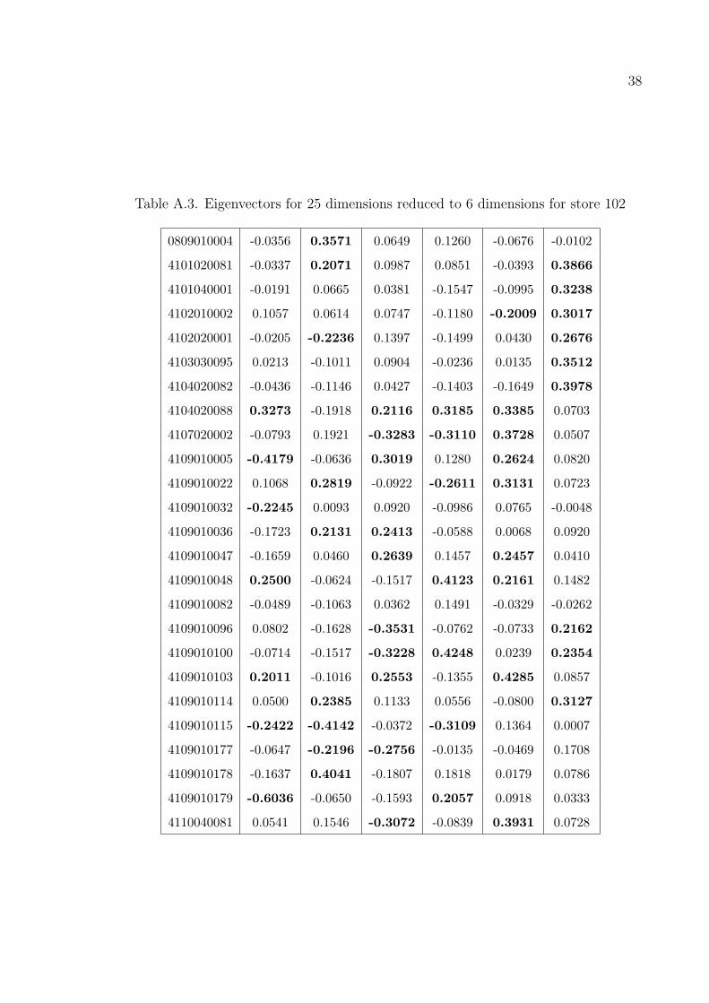
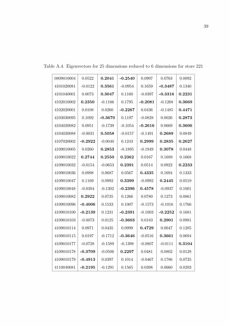
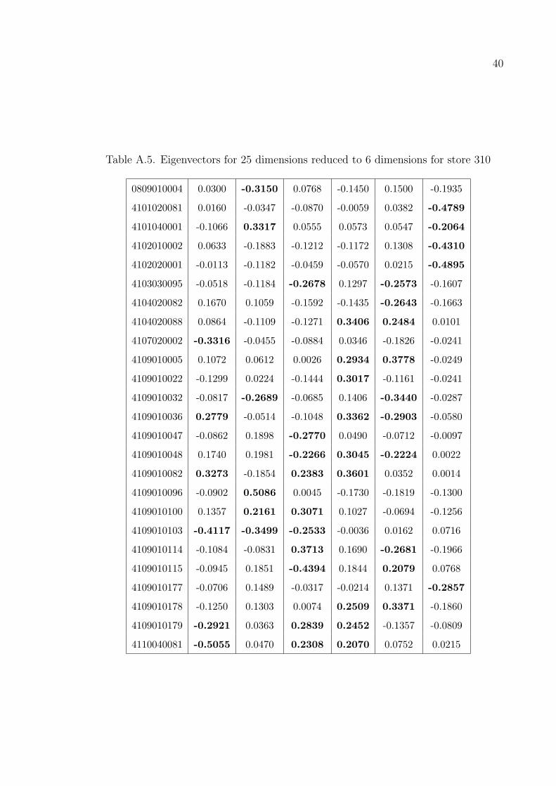
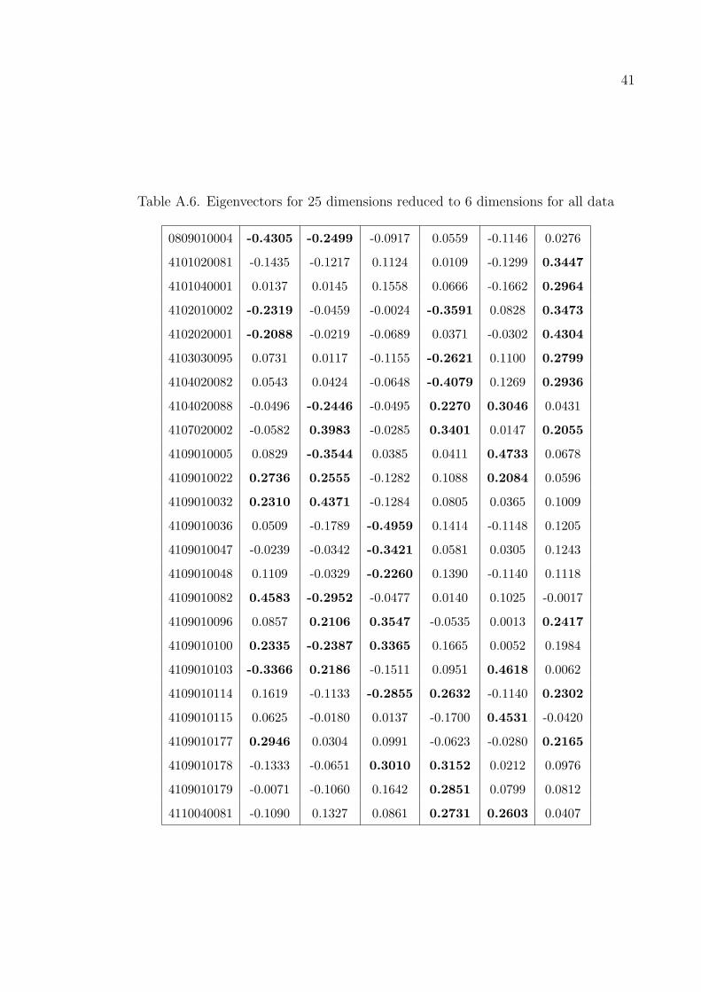
The Tables A.3–A.6 show the most important six eigenvalues on twenty five
dimensional data. The values in the left column are the item codes i.e. ID’s of items.
The numbers in bold are the important values on the vectors.
36
Table A.1. Energies in 46 dimensions
Dimensions Energy 102 Energy 221 Energy 310 Energy All
1 6.8250 4.7815 9.9395 6.6745
2 11.3923 8.8548 14.0537 10.5869
3 15.0288 12.6433 17.9653 14.2449
4 18.4215 16.2711 21.4087 17.4557
5 21.7830 19.5894 24.7100 20.4615
6 24.9176 22.7066 27.7381 23.3674
7 27.8139 25.7044 30.6874 26.1074
8 30.6485 28.5862 33.5558 28.7711
9 33.4230 31.4120 36.3564 31.3873
10 36.1070 34.1257 39.0208 33.8498
15 48.4428 46.7840 51.1320 45.2401
20 59.4534 58.0126 62.0026 55.9112
25 69.3741 68.2429 71.7639 66.0638
30 78.3538 77.3849 80.6022 75.4826
35 86.3052 85.4905 88.4495 84.2216
40 93.2828 92.7304 95.1932 92.3182
41 94.5777 94.0756 96.3892 93.8481
42 95.7872 95.4009 97.3896 95.2761
43 96.9350 96.6519 98.2534 96.6769
44 98.0012 97.8744 99.0330 98.0049
45 99.0314 98.9860 99.7608 99.0768
46 100.0000 100.0000 100.0000 100.0000
37
Table A.2. Energies in 100 dimensions
Dimensions Energy 102 Energy 221 Energy 310 Energy All
1 3.0472 2.8192 3.5550 2.8218
2 5.5569 5.1050 6.3912 5.4010
3 7.6125 7.0773 8.4756 7.3737
4 9.5986 9.0138 10.4676 9.1752
5 11.5088 10.8593 12.3956 10.7975
10 20.2175 19.3763 20.8872 17.9335
15 28.0977 27.0103 28.3342 24.2317
20 35.3155 34.1314 35.1939 30.0427
25 41.8668 40.6784 41.5633 35.5507
30 47.9009 46.7490 47.4852 40.8553
35 53.5549 52.3916 53.0675 45.9895
40 58.8126 57.7134 58.2697 51.0123
45 63.7631 62.7319 63.2102 55.8776
50 68.4620 67.4049 67.8531 60.5977
55 72.8663 71.7863 72.2717 65.1961
60 76.9672 75.9198 76.4717 69.6623
65 80.7847 79.7959 80.3553 74.0010
70 84.3274 83.4129 83.9803 78.2028
75 87.5847 86.7863 87.3854 82.2913
80 90.5923 89.9398 90.5325 86.2489
85 93.3902 92.8366 93.4252 90.0764
90 95.9369 95.5280 96.0421 93.7192
95 98.1790 97.9272 98.3514 97.1279
96 98.5790 98.3802 98.7734 97.7799
97 98.9682 98.8093 99.1325 98.4061
98 99.3459 99.2288 99.4800 99.0178
99 99.7052 99.6245 99.7890 99.5669
100 100.0000 100.0000 100.0000 100.0000
38
Table A.3. Eigenvectors for 25 dimensions reduced to 6 dimensions for store 102
0809010004 -0.0356 0.3571 0.0649 0.1260 -0.0676 -0.0102
4101020081 -0.0337 0.2071 0.0987 0.0851 -0.0393 0.3866
4101040001 -0.0191 0.0665 0.0381 -0.1547 -0.0995 0.3238
4102010002 0.1057 0.0614 0.0747 -0.1180 -0.2009 0.3017
4102020001 -0.0205 -0.2236 0.1397 -0.1499 0.0430 0.2676
4103030095 0.0213 -0.1011 0.0904 -0.0236 0.0135 0.3512
4104020082 -0.0436 -0.1146 0.0427 -0.1403 -0.1649 0.3978
4104020088 0.3273 -0.1918 0.2116 0.3185 0.3385 0.0703
4107020002 -0.0793 0.1921 -0.3283 -0.3110 0.3728 0.0507
4109010005 -0.4179 -0.0636 0.3019 0.1280 0.2624 0.0820
4109010022 0.1068 0.2819 -0.0922 -0.2611 0.3131 0.0723
4109010032 -0.2245 0.0093 0.0920 -0.0986 0.0765 -0.0048
4109010036 -0.1723 0.2131 0.2413 -0.0588 0.0068 0.0920
4109010047 -0.1659 0.0460 0.2639 0.1457 0.2457 0.0410
4109010048 0.2500 -0.0624 -0.1517 0.4123 0.2161 0.1482
4109010082 -0.0489 -0.1063 0.0362 0.1491 -0.0329 -0.0262
4109010096 0.0802 -0.1628 -0.3531 -0.0762 -0.0733 0.2162
4109010100 -0.0714 -0.1517 -0.3228 0.4248 0.0239 0.2354
4109010103 0.2011 -0.1016 0.2553 -0.1355 0.4285 0.0857
4109010114 0.0500 0.2385 0.1133 0.0556 -0.0800 0.3127
4109010115 -0.2422 -0.4142 -0.0372 -0.3109 0.1364 0.0007
4109010177 -0.0647 -0.2196 -0.2756 -0.0135 -0.0469 0.1708
4109010178 -0.1637 0.4041 -0.1807 0.1818 0.0179 0.0786
4109010179 -0.6036 -0.0650 -0.1593 0.2057 0.0918 0.0333
4110040081 0.0541 0.1546 -0.3072 -0.0839 0.3931 0.0728
39
Table A.4. Eigenvectors for 25 dimensions reduced to 6 dimensions for store 221
0809010004 0.0522 0.2041 -0.2540 0.0997 0.0763 0.0092
4101020081 -0.0122 0.3561 -0.0954 0.1659 -0.3487 0.1340
4101040001 0.0073 0.3047 0.1160 -0.0397 -0.3316 0.2231
4102010002 0.2350 -0.1166 0.1795 -0.2081 -0.1268 0.3669
4102020001 0.0108 0.0260 -0.2267 0.0436 -0.1485 0.4471
4103030095 0.1092 -0.3670 0.1197 -0.0828 0.0026 0.2873
4104020082 0.0951 -0.1739 -0.1054 -0.2616 0.0669 0.3606
4104020088 -0.0031 0.5058 -0.0157 -0.1491 0.2689 0.0849
4107020002 -0.2922 -0.0040 0.1243 0.2999 0.2835 0.2627
4109010005 0.0260 0.2853 -0.1895 -0.1949 0.3078 0.0448
4109010022 0.2744 0.2550 0.2362 0.0167 0.1689 0.1668
4109010032 -0.0154 -0.0653 0.2391 0.0514 0.0922 0.2233
4109010036 0.0998 0.0687 0.0567 0.4335 0.1694 0.1333
4109010047 0.1169 0.0992 0.3399 -0.0992 0.2445 0.0519
4109010048 -0.0394 -0.1302 -0.2396 0.4578 -0.0937 0.1001
4109010082 0.2922 0.0735 0.1266 0.0780 0.1273 0.0861
4109010096 -0.4006 0.1533 0.1007 -0.1573 -0.1016 0.1766
4109010100 -0.2139 0.1231 -0.2391 -0.1003 -0.2252 0.1681
4109010103 -0.0073 0.0125 -0.3603 0.0183 0.2901 0.0981
4109010114 0.0971 0.0435 0.0999 0.4729 0.0047 0.1205
4109010115 0.0197 -0.1712 -0.3646 -0.0516 0.3661 0.0694
4109010177 -0.0728 -0.1589 -0.1398 -0.0807 -0.0111 0.3104
4109010178 -0.3709 -0.0506 0.2297 0.0481 0.0802 0.0128
4109010179 -0.4913 0.0397 0.1014 -0.0467 0.1786 0.0735
4110040081 -0.2195 -0.1291 0.1565 0.0398 0.0660 0.0293
40
Table A.5. Eigenvectors for 25 dimensions reduced to 6 dimensions for store 310
0809010004 0.0300 -0.3150 0.0768 -0.1450 0.1500 -0.1935
4101020081 0.0160 -0.0347 -0.0870 -0.0059 0.0382 -0.4789
4101040001 -0.1066 0.3317 0.0555 0.0573 0.0547 -0.2064
4102010002 0.0633 -0.1883 -0.1212 -0.1172 0.1308 -0.4310
4102020001 -0.0113 -0.1182 -0.0459 -0.0570 0.0215 -0.4895
4103030095 -0.0518 -0.1184 -0.2678 0.1297 -0.2573 -0.1607
4104020082 0.1670 0.1059 -0.1592 -0.1435 -0.2643 -0.1663
4104020088 0.0864 -0.1109 -0.1271 0.3406 0.2484 0.0101
4107020002 -0.3316 -0.0455 -0.0884 0.0346 -0.1826 -0.0241
4109010005 0.1072 0.0612 0.0026 0.2934 0.3778 -0.0249
4109010022 -0.1299 0.0224 -0.1444 0.3017 -0.1161 -0.0241
4109010032 -0.0817 -0.2689 -0.0685 0.1406 -0.3440 -0.0287
4109010036 0.2779 -0.0514 -0.1048 0.3362 -0.2903 -0.0580
4109010047 -0.0862 0.1898 -0.2770 0.0490 -0.0712 -0.0097
4109010048 0.1740 0.1981 -0.2266 0.3045 -0.2224 0.0022
4109010082 0.3273 -0.1854 0.2383 0.3601 0.0352 0.0014
4109010096 -0.0902 0.5086 0.0045 -0.1730 -0.1819 -0.1300
4109010100 0.1357 0.2161 0.3071 0.1027 -0.0694 -0.1256
4109010103 -0.4117 -0.3499 -0.2533 -0.0036 0.0162 0.0716
4109010114 -0.1084 -0.0831 0.3713 0.1690 -0.2681 -0.1966
4109010115 -0.0945 0.1851 -0.4394 0.1844 0.2079 0.0768
4109010177 -0.0706 0.1489 -0.0317 -0.0214 0.1371 -0.2857
4109010178 -0.1250 0.1303 0.0074 0.2509 0.3371 -0.1860
4109010179 -0.2921 0.0363 0.2839 0.2452 -0.1357 -0.0809
4110040081 -0.5055 0.0470 0.2308 0.2070 0.0752 0.0215
41
Table A.6. Eigenvectors for 25 dimensions reduced to 6 dimensions for all data
0809010004 -0.4305 -0.2499 -0.0917 0.0559 -0.1146 0.0276
4101020081 -0.1435 -0.1217 0.1124 0.0109 -0.1299 0.3447
4101040001 0.0137 0.0145 0.1558 0.0666 -0.1662 0.2964
4102010002 -0.2319 -0.0459 -0.0024 -0.3591 0.0828 0.3473
4102020001 -0.2088 -0.0219 -0.0689 0.0371 -0.0302 0.4304
4103030095 0.0731 0.0117 -0.1155 -0.2621 0.1100 0.2799
4104020082 0.0543 0.0424 -0.0648 -0.4079 0.1269 0.2936
4104020088 -0.0496 -0.2446 -0.0495 0.2270 0.3046 0.0431
4107020002 -0.0582 0.3983 -0.0285 0.3401 0.0147 0.2055
4109010005 0.0829 -0.3544 0.0385 0.0411 0.4733 0.0678
4109010022 0.2736 0.2555 -0.1282 0.1088 0.2084 0.0596
4109010032 0.2310 0.4371 -0.1284 0.0805 0.0365 0.1009
4109010036 0.0509 -0.1789 -0.4959 0.1414 -0.1148 0.1205
4109010047 -0.0239 -0.0342 -0.3421 0.0581 0.0305 0.1243
4109010048 0.1109 -0.0329 -0.2260 0.1390 -0.1140 0.1118
4109010082 0.4583 -0.2952 -0.0477 0.0140 0.1025 -0.0017
4109010096 0.0857 0.2106 0.3547 -0.0535 0.0013 0.2417
4109010100 0.2335 -0.2387 0.3365 0.1665 0.0052 0.1984
4109010103 -0.3366 0.2186 -0.1511 0.0951 0.4618 0.0062
4109010114 0.1619 -0.1133 -0.2855 0.2632 -0.1140 0.2302
4109010115 0.0625 -0.0180 0.0137 -0.1700 0.4531 -0.0420
4109010177 0.2946 0.0304 0.0991 -0.0623 -0.0280 0.2165
4109010178 -0.1333 -0.0651 0.3010 0.3152 0.0212 0.0976
4109010179 -0.0071 -0.1060 0.1642 0.2851 0.0799 0.0812
4110040081 -0.1090 0.1327 0.0861 0.2731 0.2603 0.0407

42
0 10 20 30 40 50 60 70 80 90 1000
10
20
30
40
50
60
70
80
90
100Energy in 221
Per
cent
age
expl
aine
d
Number of attributes
−8 −6 −4 −2 0 2 4−2
0
2
4
6
8
10
12
Data 221
X2
X1
Figure A.1. Energy and data reduced to 2 dimensions for 25 items for store number
221
43
0 10 20 30 40 50 60 70 80 90 1000
10
20
30
40
50
60
70
80
90
100Energy in 310
Per
cent
age
expl
aine
d
Number of attributes
−4 −2 0 2 4 6 8 10−90
−80
−70
−60
−50
−40
−30
−20
−10
0
10
Data 310
X2
X1
Figure A.2. Energy and data reduced to 2 dimensions for 25 items for store number
310

44
0 10 20 30 40 50 60 70 80 90 1000
10
20
30
40
50
60
70
80
90
100Energy in All dataset
Per
cent
age
expl
aine
d
Number of attributes
−70 −60 −50 −40 −30 −20 −10 0 10−10
−5
0
5
10
15
20
All Data
X2
X1
Figure A.3. Energy and data reduced to 2 dimensions for 25 items for whole data

45
0 5 10 15 20 25 30 35 40 45 500
10
20
30
40
50
60
70
80
90
100
Number of attributes
Per
cent
age
expl
aine
dEnergy in 102
−40 −30 −20 −10 0 10 20 30 40−5
0
5
10
15
20
25
30
Data 102
X2
X1
Figure A.4. Energy and data reduced to 2 dimensions for 46 items for store number
102
46
0 5 10 15 20 25 30 35 40 45 500
10
20
30
40
50
60
70
80
90
100
Number of attributes
Per
cent
age
expl
aine
dEnergy in 221
−8 −6 −4 −2 0 2 4 6 80
2
4
6
8
10
12
Data 221
X2
X1
Figure A.5. Energy and data reduced to 2 dimensions for 46 items for store number
221
47
0 5 10 15 20 25 30 35 40 45 500
10
20
30
40
50
60
70
80
90
100
Number of attributes
Per
cent
age
expl
aine
dEnergy in 310
−15 −10 −5 0 5 10 15−140
−120
−100
−80
−60
−40
−20
0
20
Data 310
X2
X1
Figure A.6. Energy and data reduced to 2 dimensions for 46 items for store number
310
48
0 5 10 15 20 25 30 35 40 45 500
10
20
30
40
50
60
70
80
90
100
Number of attributes
Per
cent
age
expl
aine
dEnergy in All dataset
−70 −60 −50 −40 −30 −20 −10 0 10 20 30−20
0
20
40
60
80
100
120
Data All
X2
X1
Figure A.7. Energy and data reduced to 2 dimensions for 46 items for whole data
49
0 10 20 30 40 50 60 70 80 90 1000
10
20
30
40
50
60
70
80
90
100
Number of attributes
Per
cent
age
expl
aine
dEnergy in 102
−15 −10 −5 0 5 10 150
5
10
15
20
25
Data 102
X2
X1
Figure A.8. Energy and data reduced to 2 dimensions for 100 items for store number
102
50
0 10 20 30 40 50 60 70 80 90 1000
10
20
30
40
50
60
70
80
90
100Energy in 221
Per
cent
age
expl
aine
d
Number of attributes
−8 −6 −4 −2 0 2 4−2
0
2
4
6
8
10
12
Data 221
X2
X1
Figure A.9. Energy and data reduced to 2 dimensions for 100 items for store number
221

51
0 10 20 30 40 50 60 70 80 90 1000
10
20
30
40
50
60
70
80
90
100Energy in 310
Per
cent
age
expl
aine
d
Number of attributes
−4 −2 0 2 4 6 8 10−90
−80
−70
−60
−50
−40
−30
−20
−10
0
10
Data 310
X2
X1
Figure A.10. Energy and data reduced to 2 dimensions for 100 items for store number
310

52
0 10 20 30 40 50 60 70 80 90 1000
10
20
30
40
50
60
70
80
90
100Energy in All dataset
Per
cent
age
expl
aine
d
Number of attributes
−70 −60 −50 −40 −30 −20 −10 0 10−10
−5
0
5
10
15
20
All Data
X2
X1
Figure A.11. Energy and data reduced to 2 dimensions for 100 items for whole data
53
APPENDIX B: RESULTS OF K-MEANS CLUSTERING
The results in Tables B.1–B.7 are taken from the stores numbered 102, 221,
310 and the whole database and with choosing the number of items 25 and number
of clusters as 4 and 8. The numbers above the means show the percentage of the
customers belonging to that cluster. We first normalized the data acording to the
items to disable the effect of difference variances and means in the data.

54
Table B.1. Store 102 with 8 means
8-MEANS
ITEMS 54.5% 15.5% 1.6% 12.1% 1.8% 9.3% 4.2% 1%
0809010004 0.043 -0.189 -0.217 0.039 0.029 -0.026 0.099 0.226
4101020081 -0.185 -0.139 0.178 0.374 0.371 0.022 1.445 0.525
4101040001 -0.188 -0.177 -0.097 -0.083 0.014 -0.156 3.651 0.289
4102010002 -0.148 -0.108 -0.302 0.673 -0.215 -0.048 0.694 0.033
4102020001 -0.267 -0.130 0.007 0.313 0.054 1.252 0.289 -0.139
4103030095 -0.246 -0.093 0.755 0.701 -0.137 -0.083 1.320 0.669
4104020082 -0.263 -0.007 -0.293 0.855 0.090 -0.073 1.155 0.262
4104020088 -0.118 -0.030 5.655 -0.166 0.093 -0.019 -0.075 0.221
4107020002 -0.111 0.093 -0.182 0.064 1.674 0.023 0.098 0.501
4109010005 -0.233 -0.164 0.626 -0.145 0.102 1.643 0.070 0.274
4109010022 -0.054 -0.072 1.764 -0.184 0.770 -0.024 0.414 0.578
4109010032 -0.066 -0.004 -0.121 -0.136 0.099 -0.055 -0.146 6.490
4109010036 -0.045 -0.111 -0.078 0.081 -0.182 0.218 0.235 0.636
4109010047 -0.099 -0.137 0.588 -0.115 0.301 0.654 -0.084 1.723
4109010048 -0.095 -0.139 1.154 0.322 0.821 0.025 -0.001 -0.100
4109010082 -0.034 0.024 0.112 -0.096 -0.177 0.341 -0.048 -0.154
4109010096 -0.212 -0.091 -0.265 1.004 0.772 -0.183 0.349 0.108
4109010100 -0.145 -0.209 0.620 0.686 0.376 0.062 0.201 -0.230
4109010103 -0.127 0.086 0.930 -0.207 0.632 0.482 0.153 0.384
4109010114 -0.088 -0.197 -0.006 0.249 0.101 0.195 0.710 -0.119
4109010115 -0.413 1.706 -0.165 -0.253 -0.150 -0.100 0.038 0.474
4109010177 -0.217 -0.149 -0.223 1.282 -0.049 -0.166 0.150 0.006
4109010178 -0.096 -0.014 -0.072 -0.068 3.532 0.063 -0.086 -0.131
4109010179 -0.107 -0.065 -0.127 -0.065 0.014 0.848 0.027 -0.160
4110040081 -0.097 -0.139 -0.013 -0.086 5.119 -0.001 -0.132 -0.113
55
Table B.2. Store 221 with 4 means
4-MEANS
ITEMS 14, 10% 20, 70% 58, 40% 6, 80%
0809010004 -0.0728 0.0876 0.0024 -0.1364
4101020081 -0.0797 0.2355 -0.0514 -0.1099
4101040001 -0.0090 0.2740 -0.0730 -0.1884
4102010002 0.0248 0.4537 -0.1728 0.0512
4102020001 -0.1996 0.9619 -0.2735 -0.1655
4103030095 0.0697 0.4890 -0.1701 -0.1722
4104020082 0.0572 0.4369 -0.1887 0.1714
4104020088 -0.0158 -0.1275 -0.1569 1.7685
4107020002 0.0365 0.6335 -0.2564 0.1974
4109010005 0.0686 -0.0912 -0.1740 1.6295
4109010022 0.0834 0.0970 -0.1249 0.6047
4109010032 0.2018 0.4150 -0.1595 -0.3116
4109010036 0.0246 0.4751 -0.1743 0.0002
4109010047 2.0486 -0.2862 -0.3804 -0.1093
4109010048 -0.4792 0.6312 -0.0939 -0.1217
4109010082 0.0222 0.0454 -0.0836 0.5338
4109010096 -0.1274 0.0600 -0.0436 0.4563
4109010100 -0.1232 0.2837 -0.0725 0.0142
4109010103 -0.0321 0.2303 -0.0812 0.0631
4109010114 -0.1015 0.4981 -0.1253 -0.2297
4109010115 0.0512 0.1610 -0.0864 0.1456
4109010177 0.0792 0.5415 -0.1854 -0.2204
4109010178 -0.1140 -0.0616 -0.0794 1.1056
4109010179 0.0287 0.0719 -0.0691 0.3153
4110040081 -0.1086 -0.0611 -0.1304 1.5313
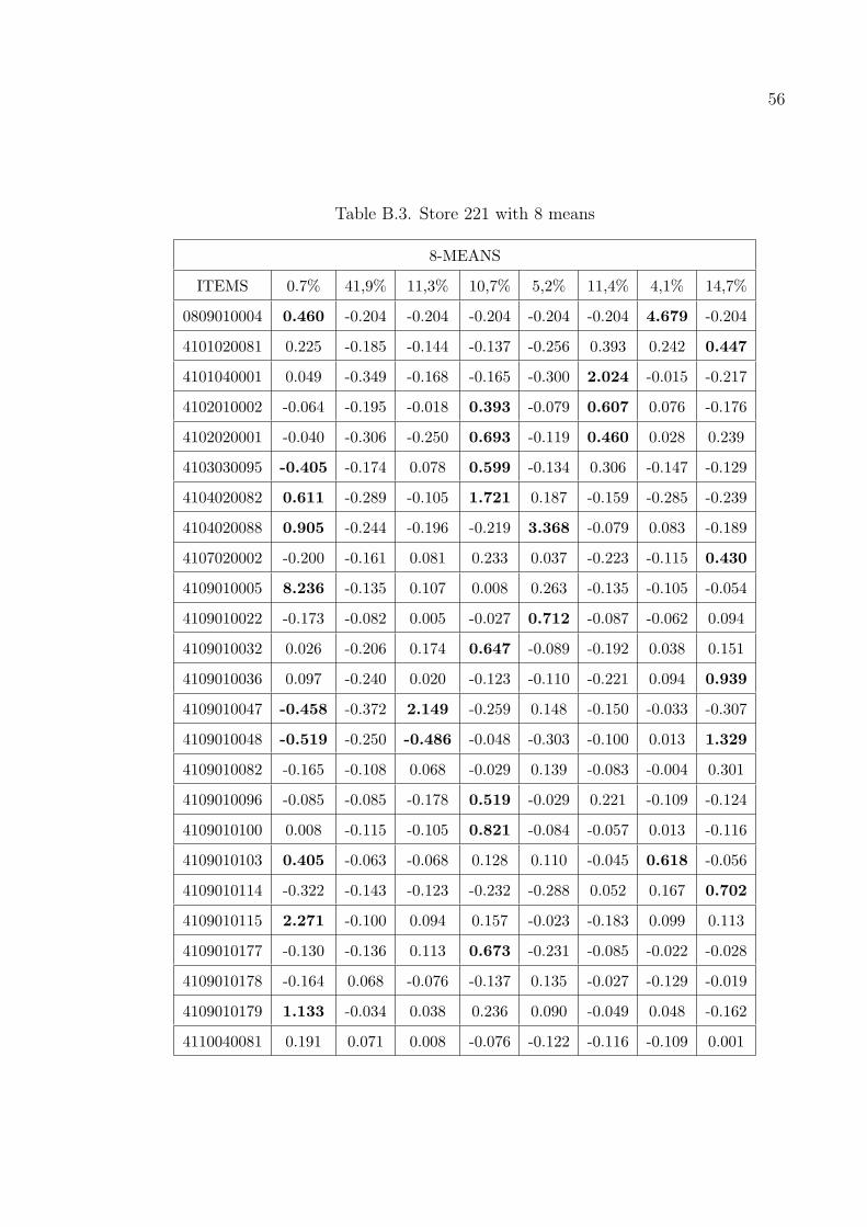
56
Table B.3. Store 221 with 8 means
8-MEANS
ITEMS 0.7% 41,9% 11,3% 10,7% 5,2% 11,4% 4,1% 14,7%
0809010004 0.460 -0.204 -0.204 -0.204 -0.204 -0.204 4.679 -0.204
4101020081 0.225 -0.185 -0.144 -0.137 -0.256 0.393 0.242 0.447
4101040001 0.049 -0.349 -0.168 -0.165 -0.300 2.024 -0.015 -0.217
4102010002 -0.064 -0.195 -0.018 0.393 -0.079 0.607 0.076 -0.176
4102020001 -0.040 -0.306 -0.250 0.693 -0.119 0.460 0.028 0.239
4103030095 -0.405 -0.174 0.078 0.599 -0.134 0.306 -0.147 -0.129
4104020082 0.611 -0.289 -0.105 1.721 0.187 -0.159 -0.285 -0.239
4104020088 0.905 -0.244 -0.196 -0.219 3.368 -0.079 0.083 -0.189
4107020002 -0.200 -0.161 0.081 0.233 0.037 -0.223 -0.115 0.430
4109010005 8.236 -0.135 0.107 0.008 0.263 -0.135 -0.105 -0.054
4109010022 -0.173 -0.082 0.005 -0.027 0.712 -0.087 -0.062 0.094
4109010032 0.026 -0.206 0.174 0.647 -0.089 -0.192 0.038 0.151
4109010036 0.097 -0.240 0.020 -0.123 -0.110 -0.221 0.094 0.939
4109010047 -0.458 -0.372 2.149 -0.259 0.148 -0.150 -0.033 -0.307
4109010048 -0.519 -0.250 -0.486 -0.048 -0.303 -0.100 0.013 1.329
4109010082 -0.165 -0.108 0.068 -0.029 0.139 -0.083 -0.004 0.301
4109010096 -0.085 -0.085 -0.178 0.519 -0.029 0.221 -0.109 -0.124
4109010100 0.008 -0.115 -0.105 0.821 -0.084 -0.057 0.013 -0.116
4109010103 0.405 -0.063 -0.068 0.128 0.110 -0.045 0.618 -0.056
4109010114 -0.322 -0.143 -0.123 -0.232 -0.288 0.052 0.167 0.702
4109010115 2.271 -0.100 0.094 0.157 -0.023 -0.183 0.099 0.113
4109010177 -0.130 -0.136 0.113 0.673 -0.231 -0.085 -0.022 -0.028
4109010178 -0.164 0.068 -0.076 -0.137 0.135 -0.027 -0.129 -0.019
4109010179 1.133 -0.034 0.038 0.236 0.090 -0.049 0.048 -0.162
4110040081 0.191 0.071 0.008 -0.076 -0.122 -0.116 -0.109 0.001
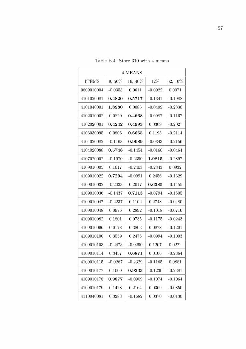
57
Table B.4. Store 310 with 4 means
4-MEANS
ITEMS 9, 50% 16, 40% 12% 62, 10%
0809010004 -0.0355 0.0611 -0.0922 0.0071
4101020081 0.4820 0.5717 -0.1341 -0.1988
4101040001 1.8980 0.0086 -0.0499 -0.2830
4102010002 0.0820 0.4668 -0.0987 -0.1167
4102020001 0.4242 0.4993 0.0309 -0.2027
4103030095 0.0806 0.6665 0.1195 -0.2114
4104020082 -0.1163 0.9089 -0.0343 -0.2156
4104020088 0.5748 -0.1454 -0.0160 -0.0464
4107020002 -0.1970 -0.2390 1.9815 -0.2897
4109010005 0.1017 -0.2403 -0.2343 0.0932
4109010022 0.7294 -0.0991 0.2456 -0.1329
4109010032 -0.2033 0.2017 0.6385 -0.1455
4109010036 -0.1437 0.7113 -0.0794 -0.1505
4109010047 -0.2237 0.1102 0.2748 -0.0480
4109010048 0.0976 0.2892 -0.1018 -0.0716
4109010082 0.1801 0.0735 -0.1175 -0.0243
4109010096 0.0178 0.3803 0.0878 -0.1201
4109010100 0.3539 0.2475 -0.0994 -0.1003
4109010103 -0.2473 -0.0290 0.1207 0.0222
4109010114 0.3457 0.6871 0.0106 -0.2364
4109010115 -0.0267 -0.2329 -0.1165 0.0881
4109010177 0.1009 0.9333 -0.1230 -0.2381
4109010178 0.9877 -0.0909 -0.1074 -0.1064
4109010179 0.1428 0.2164 0.0309 -0.0850
4110040081 0.3288 -0.1682 0.0370 -0.0130

58
Table B.5. Store 310 with 8 means
8-MEANS
ITEMS 2,4% 5,7% 2,7% 12,3% 9,9% 2,9% 55,3% 8,8%
0809010004 -0.129 -0.129 -0.129 -0.093 0.141 0.024 0.023 -0.028
4101020081 -0.253 -0.287 0.152 0.345 0.221 0.233 -0.186 0.570
4101040001 -0.470 -0.105 0.080 1.897 -0.156 0.461 -0.364 -0.167
4102010002 -0.055 -0.025 -0.247 0.000 -0.137 -0.002 -0.166 1.308
4102020001 -0.149 -0.154 0.263 0.275 0.109 0.160 -0.179 0.627
4103030095 -0.174 -0.246 -0.169 0.039 0.781 0.239 -0.195 0.476
4104020082 -0.377 -0.266 -0.025 0.189 0.102 -0.368 -0.214 1.374
4104020088 5.031 -0.087 -0.019 -0.117 -0.051 -0.035 -0.144 -0.171
4107020002 -0.235 0.044 0.144 -0.067 0.782 -0.240 -0.088 -0.156
4109010005 0.319 0.074 0.250 -0.156 -0.179 0.016 0.053 -0.133
4109010022 0.108 0.074 -0.040 -0.110 0.520 0.793 -0.110 -0.061
4109010032 -0.030 -0.082 0.005 -0.208 1.212 -0.349 -0.168 0.159
4109010036 -0.217 -0.174 0.160 -0.070 1.162 -0.245 -0.173 0.084
4109010047 -0.060 -0.064 0.125 -0.029 0.461 0.081 -0.079 0.017
4109010048 0.004 -0.141 -0.080 -0.198 1.330 -0.095 -0.142 -0.178
4109010082 0.060 -0.033 0.186 -0.169 0.166 0.106 0.000 -0.037
4109010096 -0.369 -0.120 0.043 0.292 0.013 -0.055 -0.091 0.332
4109010100 -0.052 -0.184 5.134 -0.034 -0.187 -0.210 -0.157 -0.122
4109010103 0.157 2.012 -0.311 -0.150 0.059 -0.288 -0.155 -0.036
4109010114 -0.013 0.034 0.578 0.236 0.331 0.294 -0.159 0.006
4109010115 0.166 0.174 -0.335 -0.118 0.194 -0.004 0.012 -0.187
4109010177 -0.234 -0.151 0.345 0.036 -0.268 0.876 -0.229 1.461
4109010178 0.043 -0.034 0.076 -0.100 -0.135 3.803 -0.138 -0.102
4109010179 -0.199 0.056 0.333 -0.139 0.171 2.051 -0.102 -0.111
4110040081 -0.116 2.719 -0.190 -0.095 -0.167 -0.038 -0.181 -0.197
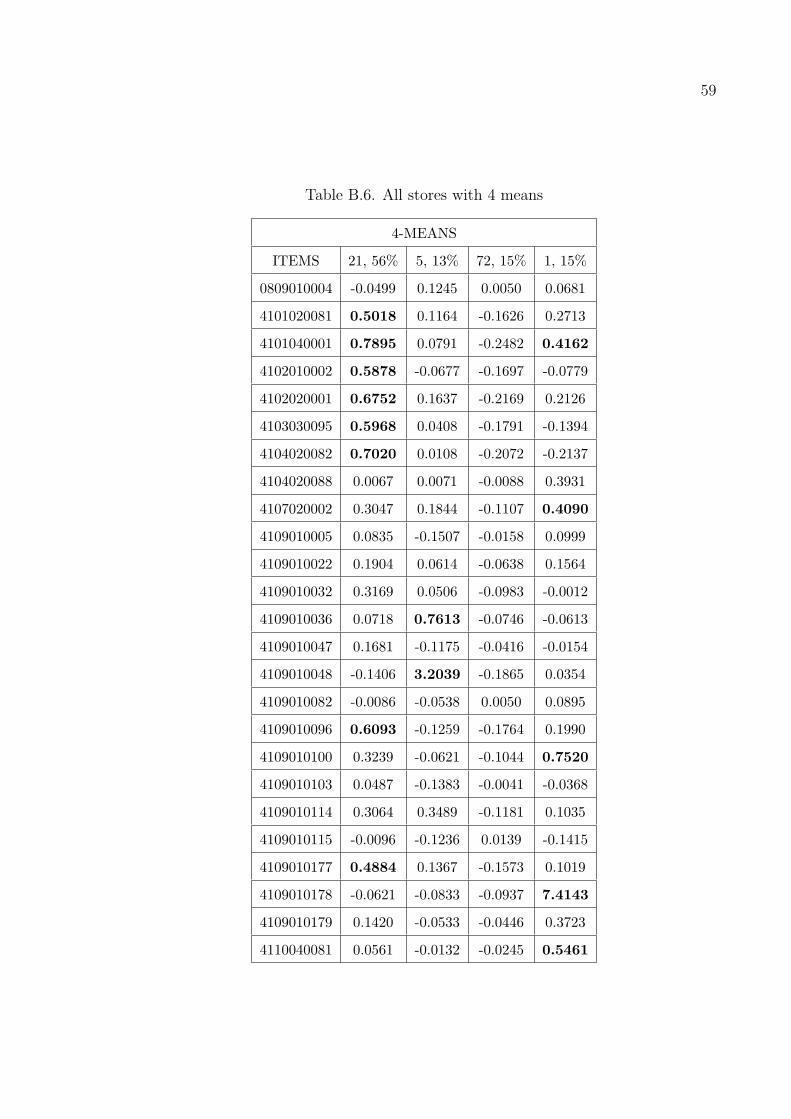
59
Table B.6. All stores with 4 means
4-MEANS
ITEMS 21, 56% 5, 13% 72, 15% 1, 15%
0809010004 -0.0499 0.1245 0.0050 0.0681
4101020081 0.5018 0.1164 -0.1626 0.2713
4101040001 0.7895 0.0791 -0.2482 0.4162
4102010002 0.5878 -0.0677 -0.1697 -0.0779
4102020001 0.6752 0.1637 -0.2169 0.2126
4103030095 0.5968 0.0408 -0.1791 -0.1394
4104020082 0.7020 0.0108 -0.2072 -0.2137
4104020088 0.0067 0.0071 -0.0088 0.3931
4107020002 0.3047 0.1844 -0.1107 0.4090
4109010005 0.0835 -0.1507 -0.0158 0.0999
4109010022 0.1904 0.0614 -0.0638 0.1564
4109010032 0.3169 0.0506 -0.0983 -0.0012
4109010036 0.0718 0.7613 -0.0746 -0.0613
4109010047 0.1681 -0.1175 -0.0416 -0.0154
4109010048 -0.1406 3.2039 -0.1865 0.0354
4109010082 -0.0086 -0.0538 0.0050 0.0895
4109010096 0.6093 -0.1259 -0.1764 0.1990
4109010100 0.3239 -0.0621 -0.1044 0.7520
4109010103 0.0487 -0.1383 -0.0041 -0.0368
4109010114 0.3064 0.3489 -0.1181 0.1035
4109010115 -0.0096 -0.1236 0.0139 -0.1415
4109010177 0.4884 0.1367 -0.1573 0.1019
4109010178 -0.0621 -0.0833 -0.0937 7.4143
4109010179 0.1420 -0.0533 -0.0446 0.3723
4110040081 0.0561 -0.0132 -0.0245 0.5461
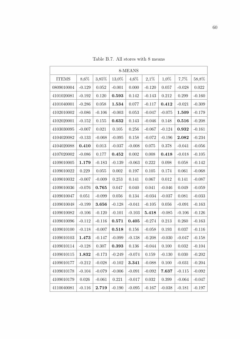
60
Table B.7. All stores with 8 means
8-MEANS
ITEMS 8,6% 3,85% 13,0% 4,6% 2,1% 1,0% 7,7% 58,8%
0809010004 -0.129 0.052 -0.001 0.000 -0.120 0.057 -0.028 0.022
4101020081 -0.192 0.120 0.593 0.142 -0.143 0.212 0.299 -0.160
4101040001 -0.286 0.058 1.534 0.077 -0.117 0.412 -0.021 -0.309
4102010002 -0.086 -0.106 -0.003 0.053 -0.047 -0.075 1.509 -0.179
4102020001 -0.152 0.155 0.632 0.143 -0.046 0.148 0.516 -0.208
4103030095 -0.007 0.021 0.105 0.256 -0.067 -0.124 0.932 -0.161
4104020082 -0.133 -0.068 -0.095 0.158 -0.072 -0.196 2.082 -0.234
4104020088 0.410 0.013 -0.037 -0.008 0.075 0.378 -0.041 -0.056
4107020002 -0.086 0.177 0.452 0.002 0.008 0.418 -0.018 -0.105
4109010005 1.179 -0.183 -0.139 -0.063 0.222 0.098 0.058 -0.142
4109010022 0.229 0.055 0.002 0.197 0.105 0.174 0.061 -0.068
4109010032 -0.007 -0.009 0.253 0.141 0.067 0.012 0.141 -0.087
4109010036 -0.076 0.765 0.047 0.040 0.041 -0.046 0.049 -0.059
4109010047 0.051 -0.099 0.056 0.134 -0.034 -0.037 0.081 -0.033
4109010048 -0.199 3.656 -0.128 -0.041 -0.105 0.056 -0.091 -0.163
4109010082 -0.106 -0.120 -0.101 -0.103 5.418 -0.085 -0.106 -0.126
4109010096 -0.112 -0.116 0.571 0.405 -0.274 0.213 0.260 -0.163
4109010100 -0.118 -0.007 0.518 0.156 -0.058 0.193 0.037 -0.116
4109010103 1.473 -0.147 -0.099 -0.138 -0.208 -0.030 -0.047 -0.158
4109010114 -0.128 0.307 0.393 0.136 -0.044 0.100 0.032 -0.104
4109010115 1.832 -0.173 -0.249 -0.074 0.159 -0.130 0.030 -0.202
4109010177 -0.212 -0.028 -0.102 3.341 -0.088 0.100 -0.031 -0.204
4109010178 -0.104 -0.079 -0.006 -0.091 -0.092 7.637 -0.115 -0.092
4109010179 0.026 -0.061 0.221 -0.017 0.032 0.399 -0.064 -0.047
4110040081 -0.116 2.719 -0.190 -0.095 -0.167 -0.038 -0.181 -0.197
61
REFERENCES
1. Agrawal, R., T. Imielinski and A. N. Swami, “Mining Association Rules between
Sets of Items in Large Databases”, Proceedings of the 1993 ACM SIGMOD In-
ternational Conference on Management of Data, pp. 207–216, Washington, D.C.,
May 1993.
2. Agrawal, R. and R. Srikant, “Fast Algorithms for Mining Association Rules in
Large Databases”, Proceedings of the 20th International Conference on Very Large
Data Bases (VLDB), Santiago, Chile, September 1994.
3. Fang, M., N. Shivakumar, H. Garcia-Molina, R. Motwani and J. Ullman, “Comput-
ing Iceberg Queries Efficiently”, Proceedings of the 24th International Conference
on Very Large Data Bases (VLDB), pp. 299–310, August 1998.
4. Toivonen H., “Sampling Large Databases for Association Rules”, Proceedings of
the 22nd International Conference on Very Large Data Bases (VLDB), 1996.
5. Sarasere, A., E. Omiecinsky and S. Navathe, “An Efficient Algorithm for Min-
ing Association Rules in Large Databases”, Proceedings of the 21st International
Conference on Very Large Data Bases (VLDB), Zurich, Switzerland, September
1995.
6. Fu, A., R. Kwong and J. Tang, “Mining N-most Interesting Itemsets”, Proceed-
ings of the 12th International Symposium on Methodologies for Intelligent Systems
(ISMIS), Springer-Verlag, LNCS, Charlotte, North Carolina, USA, October 2000.
7. Hu, Z., W. Chin and M. Takeichi, “Calculating a new data mining algorithm
for market basket analysis”, Proceedings of the Second International Workshop
on Practical Aspects of Declarative Languages (PADL’00), Springer Verlag, LNCS
1753, Boston, Massachusetts, pp. 169–184, January 2000.
62
8. Hipp, J., A. Myka, R. Wirth and U. Guntzer, “A New Algorithm for Faster Mining
of Generalized Association Rules”, Proceedings of the 2nd European Symposium on
Principles of Data Mining and Knowledge Discovery (PKDD ’98), Nantes, France,
pp. 74–82, September 1998.
9. Kan, D. C., “An Adaptive Algorithm for Mining Association Rules on Shared
Memory Parallel Machines”, Distributed and Parallel Databases, Vol. 9, pp. 99–
132, 2001.
10. Agrawal, R. and J. Shafer, “Parallel Mining of Association Rules”, IEEE Trans-
actions On Knowledge And Data Engineering, Vol. 8, 1996.
11. Cheung, D., J. Han, V. Ng, A. Fu and Y. Fu, “A Fast Distributed Algorithm
for Mining Association Rules”, Proceedings of the 1996 International Conference
on Parallel and Distributed Information Systems, Miami Beach, Florida, USA,
December 1996.
12. Zaki, M., “Parallel and distributed association mining: A survey”, IEEE Concur-
rency, special issue on Parallel Mechanisms for Data Mining, Vol. 7, No. 4, pp.
14–25, December 1999.
13. Ganti, V., J. Gehrke and R. Ramakrishnan, “Mining Very Large Databases”, IEEE
Computer, Vol. 32, No. 8, pp. 6875, August 1999.
14. Hipp, J., U. Guntzer and G. Nakhaeizadeh, “Algorithms for Association Rule
Mining – A General Survey and Comparison”, SIGKDD Explorations, Vol. 2,
2000.
15. A. C. Rancher, Methods of Multivariate Analysis, John Wiley and Sons, New York,
1995.
16. Duda, R., O. and P. E. Hart, Pattern Classification and Scene Analysis, John
Wiley and Sons, 1973.
63
REFERENCES NOT CITED
Brin, S., R. Motwani and J. D. Ullman and S. Tsur, “Dynamic itemset counting and
implication rules for market basket data”, Proceedings of the ACM SIGMOD In-
ternational Conference on Management of Data, Vol. 26, No. 2, pp. 255–264,
New York, May 1997.
Han, E., G. Karypis and V. Kumar, “Scalable parallel data mining for association
rules”, IEEE Transactions on Knowledge and Data Engineering, 1999.
Han, J. and Y. Fu, “Mining Multiple-Level Association Rules in Large Databases”,
IEEE Transactions on Knowledge and Data Engineering, Vol. 11, pp. 798–804,
1999.
Hipp, J., U. Guntzer and G. Nakhaeizadeh, “Mining Association Rules: Deriving a
Superior Algorithm by Analysing Today’s Approaches”, Proceedings of the 4th
European Conference on Principles and Practice of Knowledge Discovery, Lyon,
France, September 2000.
Holsheimer, M., M. L. Kersten, H. Mannila and H. Toivonen, “A perspective on
databases and data mining”, Proceedings of the First International Conference
on Knowledge Discovery and Data Mining (KDD’95), pp. 150 – 155. Montreal,
Canada: AAAI Press.
Kwon, Y., R. Nakanishi, M. Ito and M. Nakanishi, “Computational Complexity of
Finding Meaningful Association Rules”, IEICE Transaction Fundamentals, Vol.
E82-A, No.9, pp. 1945–1952, September 1999.
Lamport, L., LaTeX: A Document Preperation System, Addison-Wesley, Reading, Mas-
sachusetts, 1986.
64
Mannila, H., H. Toivonen and A. Verkamo, “Improved Methods for Finding Associ-
ation Rules”, AAAI Workshop on Knowledge Discovery, pp. 181–192, Seattle,
Washington, July 1994.
Ramaswamy, S., S. Mahajan and A. Silberschatz, “On the Discovery of Interesting
Patterns in Association Rules”, Proceedings of the 24th International Conference
on Very Large Databases, pp. 368–379, August 1998.
Srikant, R. and R. Agrawal, “Mining Quantitative Association Rules in Large Rela-
tional Tables”, Proceedings of ACM SIGMOD International Conference on Man-
agement of Data, pp. 1–12, Montreal, Canada, 1996.
Tsur, D., J. D. Ullman, S. Abiteboul, C. Clifton, R. Motwani, S. Nestorov and A.
Rosenthal, “Query flocks: A generalization of association-rule mining”, Proceed-
ings of ACM SIGMOD International Conference on Management of Data, pp.
1–12, Seattle, Washington, June 1998.
Zhu, H., On-Line Analytical Mining of Association Rules, MS thesis, School of Com-
puting Science, Simon Fraser University, December 1998.