marineresearch - university of virginiafaculty.virginia.edu/berg/journals/modeling/berg et al 2007...
TRANSCRIPT

Journal ofMARINE RESEARCHVolume 65 Number 3
A fast numerical solution to the general mass-conservationequation for solutes and solids in aquatic sediments
by Peter Berg1 Dennis Swaney2 Soslashren Rysgaard3 Bo Thamdrup4 andHenrik Fossing5
ABSTRACTMathematical modeling of species transformations in aquatic sediments is usually based on
numerical solutions to the same general one-dimensional mass-conservation equation and is likely torequire substantial computation time In this paper we present a fast numerical solution to thisequation The solution is suited for both single and multi-component models and it is based on animplicit control volume discretization of the general mass-conservation equation The solutionconsists of two algorithms one that decomposes the discretization matrix once and one thatsubsequently produces multiple solutions with minimal computational effort A unique feature ofthese algorithms is that values of boundary conditions can vary as a simulation progresses withoutrequiring new decompositions of the discretization matrix This feature can reduce computation timesignificantly relative to commonly used procedures for modeling dynamic systems Finally wepresent four examples in which the numerical solution is applied to specific problems From theseexamples guidelines are derived for the discretization in space and time required to obtain precisesolutions of the general mass-conservation equation
1 Introduction
The numerical mathematical models that are being used extensively to study biogeochemi-cal transformations in aquatic sediments typically rely on a one-dimensional mass-
1 Department of Environmental Sciences University of Virginia Charlottesville Virginia 22903 USAemail pb8nvirginiaedu
2 Department of Ecology and Evolutional Biology Cornell University Ithaca New York 14853 USA3 Greenland Institute of Natural Resources Kiviog 2 Box 570 3900 Nuuk Greenland4 Danish Center for Earth System Science Institute of Biology University of Southern Denmark Campusvej
55 DK-5230 Odense M Denmark5 National Environmental Research Institute Aarhus University Department of Marine Ecology Vejlsoslashvej
25 DK 8600 Silkeborg Denmark
Journal of Marine Research 65 317ndash343 2007
317
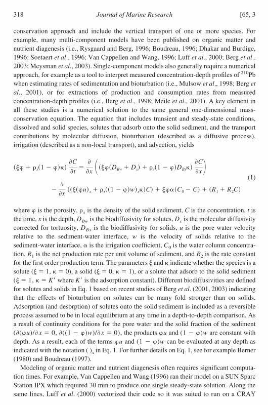
conservation approach and include the vertical transport of one or more species Forexample many multi-component models have been published on organic matter andnutrient diagenesis (ie Rysgaard and Berg 1996 Boudreau 1996 Dhakar and Burdige1996 Soetaert et al 1996 Van Cappellen and Wang 1996 Luff et al 2000 Berg et al2003 Meysman et al 2003) Single-component models also generally require a numericalapproach for example as a tool to interpret measured concentration-depth profiles of 210Pbwhen estimating rates of sedimentation and bioturbation (ie Mulsow et al 1998 Berg etal 2001) or for extractions of production and consumption rates from measuredconcentration-depth profiles (ie Berg et al 1998 Meile et al 2001) A key element inall these studies is a numerical solution to the same general one-dimensional mass-conservation equation The equation that includes transient and steady-state conditionsdissolved and solid species solutes that adsorb onto the solid sediment and the transportcontributions by molecular diffusion bioturbation (described as a diffusive process)irrigation (described as a non-local transport) and advection yields
s1 C
t
x DBw Ds s1 DBsC
x
xux s1 wxC C0 C R1 R2C
(1)
where is the porosity s is the density of the solid sediment C is the concentration t isthe time x is the depth DBw is the biodiffusivity for solutes Ds is the molecular diffusivitycorrected for tortuosity DBs is the biodiffusivity for solids u is the pore water velocityrelative to the sediment-water interface w is the velocity of solids relative to thesediment-water interface is the irrigation coefficient C0 is the water column concentra-tion R1 is the net production rate per unit volume of sediment and R2 is the rate constantfor the first order production term The parameters and indicate whether the species is asolute ( 1 0) a solid ( 0 1) or a solute that adsorb to the solid sediment( 1 K where K is the adsorption constant) Different biodiffusivities are definedfor solutes and solids in Eq 1 based on recent studies of Berg et al (2001 2003) indicatingthat the effects of bioturbation on solutes can be many fold stronger than on solidsAdsorption (and desorption) of solutes onto the solid sediment is included as a reversibleprocess assumed to be in local equilibrium at any time in a depth-to-depth comparison Asa result of continuity conditions for the pore water and the solid fraction of the sediment((u) x 0 ((1 )w) x 0) the products u and (1 )w are constant withdepth As a result each of the terms u and (1 )w can be evaluated at any depth asindicated with the notation ( )x in Eq 1 For further details on Eq 1 see for example Berner(1980) and Boudreau (1997)
Modeling of organic matter and nutrient diagenesis often requires significant computa-tion times For example Van Cappellen and Wang (1996) ran their model on a SUN SparcStation IPX which required 30 min to produce one single steady-state solution Along thesame lines Luff et al (2000) vectorized their code so it was suited to run on a CRAY
318 [65 3Journal of Marine Research
vector processor in order to reduce computation time The fact that such models usually arerun numerous times when applied to specific sediments or when used in analysisunderscores the importance of choosing the numerical solution algorithm carefullyModels used as interpretation tools can also require substantial computational effort Forexample the procedure PROFILE (Berg et al 1998) often simulates 106-107 independentsteady-state profiles in the interpretation of a single measured concentration-depth profile
This paper presents a numerical solution to Eq 1 that is developed specifically tominimize computation time The algorithm is suited to both single and multi-componentmodels and when utilized it can reduce computation time significantly relative to that ofcommonly used procedures For that reason it allows models as outlined above to beimplemented on standard microcomputers (desktop and laptop computers) without result-ing in prohibitive computation times
2 Numerical solution
The numerical solution to Eq 1 is based on a control volume approach (Patankar 1980)and relies on a separation of the calculation domain into N control volumes each containinga grid point at its center (Fig 1) It is assumed that the variation in space and time ofconcentration C is described by piecewise continuous profiles which are uniquelydetermined when the grid point values of C are known A discretization equation is derivedusing these profiles in an integration of Eq 1 over a time step and a control volume Oneclear advantage of this control volume approach is that mass-conservation is fulfilledexactly in the discretization equation
a Discretization equation
The user-defined control volumes comprising the calculation domain can vary withdepth allowing a fine resolution to be used near the sediment-water interface where themost pronounced gradients and second derivatives of concentrations are expected Thethickness of control volumes 1 and N are zero by definition (Fig 1) If a diffusive boundarylayer is included in the calculation domain a control volume indexed M with a thickness ofzero marks the sediment-water interface If this control volume separation is used formulti-component models involving both dissolved and solid species solute concentrationsare described for control volume 1 to N while concentrations of solids are found for controlvolume M to N
The integration of Eq 1 over a time step from time t to t 13t and over control volumej from xj12 to xj12 yields
xj12
xj12 t
t13t
H1
C
tdt dx
xj12
xj12 t
t13t
x H2
C
x H3C
H4C0 C R1 R2Cdt dx
(2)
2007] 319Berg et al Fast solution to mass-conservation equation
where
H1 s1
H2 DBw Ds s1 DBs
H3 ux s1 wx(3)
H4
The variables H1 H2 and H4 can vary with depth while H3 as a result of continuity alwayswill be constant with depth
In order to perform the integration in Eq 2 it is now assumed that H1 H2 H3 H4 R1and R2 are constant throughout the time step and that the grid point values of H1 H4 R1and R2 prevail throughout the control volume as representative mean values The latterassumption is not needed for H2 and H3 because these variables are not integrated over thecontrol volume With these assumptions Eq 2 gives
Figure 1 Separation of the water-sediment column into control volumes for a situation when thediffusive boundary layer D is included in the calculations Note that size of control volume 1 Mand N are zero
320 [65 3Journal of Marine Research
H1 jCjn1 Cj
n13xj t
t13t H2
C
x H3C
j12
H2
C
x H3C
j12
H4jC0 Cj R1 j R2 jCj13xjdt
(4)
where Cjn is the old (known) grid point value of C at time t and Cj
n1 is the new (unknown)grid point value of C at time t 13t
The second term on the right side of Eq 4 (H2C x H3C)j1 2 represents thecombined diffusive-advective flux Jj1 2 over the boundary between control volume j-1and j (Fig 1) It has long been known that a straightforward central difference approxima-tion of Jj1 2 inevitably leads to numerical instability when modeling advection-dominated systems (Courant et al 1952) For that reason researchers have suggestedapproximations of Jj1 2 that ensure unconditionally stable schemes (ie Courant et al1952 Spalding 1972 Fiadeiro and Veronis 1977 Patankar 1980 1981 Berg 1985)Some of the most successful schemes were derived as approximations to the analyticalsolution to the one-dimensional steady state mass-conservation equation accounting fortransport by diffusion and advection These schemes were defined through the 1970s andearly 1980s and their success was evaluated not only in terms of how well theyapproximated this analytical solution but also how fast they could be evaluated numeri-cally Because computer processors have changed radically since then the relative utility ofthese evaluation schemes have changed as well For this reason we compare theperformance of a selection of the most popular schemes on a modern microcomputer inAppendix A
Common to all these schemes is the expression of flux Jj1 2 as
Jj12 F1 jCj F2 jCj1 (5)
and the individual schemes are defined through their definition of F1 j and F2 j which arederived in details for these schemes in Appendix A Combining Eqs 4 and 5 gives
H1 jCjn1 Cj
n13xj t
t13t
F1 j1Cj1 F2 j1Cj F1 jCj F2 jCj1
H4jC0 Cj R1 j R2 jCj13xjdt
(6)
When approximating the time integral in Eq 6 it is necessary to assume how all thetime-dependent terms vary from time t to t 13t The time integral of Cj can be expressedas ((1 )Cj
n Cjn1)13t where is a weighting factor and different schemes will
result depending on the value of With 0 an explicit scheme is obtained while 1leads to an implicit scheme With 1frasl2 the Crank-Nicolson scheme a well-knownhybrid of the explicit and the implicit scheme is obtained The implicit scheme is chosenhere for the following reasons Firstly it leads to a versatile numerical solution allowing
2007] 321Berg et al Fast solution to mass-conservation equation
transient solutions to be found using appropriately sized time steps and at the same timeallowing steady-state solutions to linear problems to be produced with minimal computa-tional effort in one large time step Secondly the implicit scheme is especially attractive inone-dimensional formulations when computation time is of concern While the number ofnumeric operations per time step in the explicit Crank-Nicolson and implicit scheme issimilar a restrictive upper limit exists for the time steps in the explicit scheme Whenviolated numerical instability occurs For example in diffusion-dominated systems thiscritical time step equals 1
213x2H1H2 where H1 and H2 are given by Eq 3 In models of
organic matter and nutrient diagenesis where oxygen usually is a key component thattypically penetrates only a few mm into the sediments a 13x of 001 cm is required toaccurately describe the oxygen profile With typical values of H1 and H2 of 08 and105 cm2 s1 the critical time step is 4 s for the explicit scheme Such small time steps willlead to prohibitive computation times when multiple-year simulations are required Upperlimits to the time step obviously also exist for the implicit scheme in such simulations butthey are of a different nature and are generally markedly less restrictive For example inmulti-component models fast non-linear reactions between species can restrict the size ofthe time steps that can be used However in such modeling exercises performed withrealistic reaction rate constants time steps on the order of 1 h are usually sufficient toensure an accurate numerical solution as we demonstrate in an example below As theresult of the explicit element in the Crank-Nicolson scheme it can depending on theapplication also suffer from restrictive demands on the time step As a simple example ofthis it is not possible to produce steady-state solutions to linear problems in one large timestep as is the case with the implicit scheme
The implicit time integration in Eq 6 gives
H1 jCjn1 Cj
n13xj
13t F1 j1C j1
n1 F2 j1C jn1 F1 jC j
n1 F2 j C j1n1
H4jC0 C jn113xj R1 j R2 jC j
n113xj
(7)
which gives the following tri-diagonal system of equations
AAjCj1n1 BBjCj
n1 CCjCj1n1 DDj (8)
where the coefficients are defined as
AAj F2 j
BBj F1 j F2 j1 H4j13xj R2 j13xj H1 j
13xj
13t
CCj F1 j1
DDj H1 j
13xj
13tCj
n H4jC013xj R1 j13xj
(9)
322 [65 3Journal of Marine Research
The control volume spanning 13xj is included deliberately as a factor in Eq 9 rather than adenominator allowing 13xj to equal zero
b Boundary conditions
The boundary conditions that bring closure to the tri-diagonal system of equations(Eq 7) are imposed implicitly through control volume L and N where L equals either 1 orM depending on how the calculation domain is separated into control volumes (Fig 1) Forcontrol volume L and N Eq 8 simplifies to
BBLCLn1 CCLCL1
n1 DDL (10)
and
AANCN1n1 BBNCN
n1 DDN (11)
The coefficients BBL CCL DDL AAN BBN and DDN are given values depending on thekind of boundary conditions imposed Three types of boundary conditions are possible aknown concentration a known flux and a known concentration gradient The assignmentof values to BBL CCL DDL AAN BBN and DDN depending on the type and value of theboundary conditions are outlined in Table 1 The unique set of boundary concentrationsCL
n1 and CNn1 which ensures that the desired boundary conditions are imposed is
obtained when the tri-diagonal system of equations (Eqs 8 10 11) is solved
c Solution of tri-diagonal system of equations
Several models of biogeochemical transformations in aquatic sediments rely on implicitschemes In these models the tri-diagonal system of equations is typically solved byGaussian elimination numerous times in a single simulation (ie Dhakar and Burdige1996 Van Cappellen and Wang 1996) using for example the Thomas algorithm (iePatankar 1980 Huyakorn and Pinder 1983) Rather than performing this straightforward
Table 1 Definition of coefficients BBL CCL DDL AAN BBN and DDN in Eq 10 and 11 dependingon the imposed type and value of boundary condition
Upper boundary condition BBL CCL DDL
Known concentration 1 0 The known concentrationKnown flux F2L1 F1L1 The known fluxKnown gradient 213xL1 213xL1 The known gradient
Lower boundary condition AAN BBN DDN
Known concentration 0 1 The known concentrationKnown flux F2N F1N The known fluxKnown gradient 213xN1 213xN1 The known gradient
2007] 323Berg et al Fast solution to mass-conservation equation
Gaussian elimination in every time step a significant reduction in computation time can beobtained as follows
The coefficient DDj in the tri-diagonal system of equations (Eq 9 Table 1) willtypically vary from time step to time step in most applications simply because DDj
contains the concentration Cjn at the old time level t In contrast the coefficients AAj BBj
and CCj are likely to be constant throughout the simulation (Eq 9 Table 1) or at least varyat such a slow rate that it is appropriate to treat them as constants through manyconsecutive time steps An example of this is dynamic simulations based on time steps onthe order of minutes and where much slower seasonal temperature variations will affectvariables such as molecular diffusivities and thus AAj BBj and CCj In such simulationsit is clearly a good approximation only to update or recalculate the coefficients AAj BBj
and CCj on a weekly or monthly basis This characteristic can be taken advantage of toreduce the computational effort significantly in successive solutions of the tri-diagonalsystem of equations by decomposing the discretization matrix only once or only with timeintervals where AAj BBj and CCj vary markedly This is done by reformulating theThomas algorithm
The forward substitution in the Thomas algorithm where Eqs 8 10 and 11 are solved inthe interval L j N yields (ie Patankar 1980 Huyakorn and Pinder 1983)
PPL CCL
BBL QQL
DDL
BBL
PPj CCj
BBj AAjPPj1
QQj DDj AAjQQj1
BBj AAjPPj1
j L 1 3 N 1 (12)
QQN DDN AANQQN1
BBN AANPPN1
where PPj and QQj are decomposition variables and AAj BBj CCj and DDj are definedeither by Eq 9 or in Table 1 The following back substitution that gives the values of Cj
n1
yields
CNn1 QQN
(13)Cj
n1 PPjCj1n1 QQj j N 1 3 L
The significant gain in computational efficiency is now achieved by rewriting Eq 12 sothat DDj is kept out of the forward substitution by defining an additional decompositionvariable NNj as follows
324 [65 3Journal of Marine Research
NNL 1
BBL PPL CCLNNL
NNj 1
BBj AAjPPj1
PPj CCjNNj
j L 1 3 N 1 (14)
NNN 1
BBN AANPPN1
With this modification the back substitution that gives the values of Cjn1 then yields
QQL DDLNNL
QQj DDj AAjQQj1NNj j L 1 3 N(15)
CNn1 QQN
Cjn1 PPjCj1
n1 QQj j N 1 3 L
There are 5(N L) 1 numeric operations in Eq 15 approximately half the numberused in the original Thomas algorithm (10(N L) 1) Because multiplications arecomputationally less costly to perform than divisions the overall result is that Eq 15 are25 times faster to execute than those of the original Thomas algorithm on a 20 GHzPentium M PC
Another important and unique feature of this numerical solution is that the type ofboundary condition is introduced through BBL CCL AAN and BBN (Table 1) while thevalues of the boundary condition are imposed through DDL and DDN This characteristicallows the values of boundary conditions to vary as a simulation progresses withoutrequiring new decompositions of the discretization matrix
The coefficient DDj (Eq 9) must be calculated in every time step This is done mosteffectively as
DDj EEjCjn FFjC0 R1 j13xj (16)
where EEj and FFj are defined as
EEj H1 j
13xj
13tand FFj H4 j13xj (17)
which with the definitions of H1 j and H4 j (Eq 3) typically need only be evaluated onceIn summary it is convenient to calculate the coefficients given by Eqs 3 9 and 17 and
perform the new forward substitution given by Eq 14 in one algorithm We have namedthis algorithm CONSTANTS and its content is summarized in Appendix B The algorithmincludes five optional expressions for the molecular sediment diffusivity (Ds) as a functionof porosity and diffusivity in water The two first were originally defined by Ullman andAller (1982) the third and fourth were given by Iversen and Joslashrgensen (1993) and the fifth
2007] 325Berg et al Fast solution to mass-conservation equation
was defined by Boudreau (1997) The output from CONSTANTS are input to the secondalgorithm CNEW which performs the back substitution (Eq 15) leading to the newconcentrations every time it is utilized The content of CNEW is summarized in Appendix C
3 Applications and examples
The numerical solution separated into the two algorithms CONSTANTS and CNEW israther versatile and can be used to simulate steady state dynamic linear and nonlinearproblems that further can involve one or more dissolved or solid species The outlinedfeatures of the solution are particularly beneficial in applications where long computationtimes are of concern
Four example applications of the algorithm are presented below representing computa-tional gains achieved in diverse problems The first three focus on rather simple cases forwhich analytical solutions exist They also serve as a test of the numerical solution and asan illustration of the discretization in depth (and in time for transient problems) required toobtain accurate solutions In the last example the solution is implemented in a dynamicmulti-component and nonlinear model of organic matter and nutrient diagenesis in aspecific sediment This example illustrates clearly the significant advantages that can beachieved in terms of short computation times when applying the numerical solution tomodels where components with very different time constants require relatively small timesteps combined with long simulation times to produce quasi-stationary solution on a yearto year basis All examples are coded in FORTRAN 90 and the simulations are performedin double precision
a Example 1
Four types of solute transport molecular diffusion bioturbation irrigation and advec-tion are represented in Eq 1 An analytical solution to the equation is possible understeady-state conditions if advection and first-order production terms are neglected and if Ds DBw and R1 are assumed to be constant with depth Under these conditions Eq 1simplifies to
DBw Dsd2C
dx2 C0 C R1 0 (18)
which has the solution
C A exp
DBw Dsx B exp
DBw Dsx
C0 R1
(19)
where A and B are arbitrary constants (Boudreau 1997)Berg et al (1998) calculated a hypothetical O2 profile in the depth interval from 005
to 10 cm assuming constant consumption rates (R1) of 0004 and 0012 nmol cm3 s1 forthe depth intervals of 0 to 075 and 075 to 10 cm and then applying Eq 19 to each of these
326 [65 3Journal of Marine Research
intervals In the diffusive boundary layer (D) from 005 to 0 cm the solution simplifiesto a straight line It was further assumed that the O2 concentration equals 0 at 1 cm depthsand below Finally values of DBw Ds and of 075 3 106 cm2 s1 9 106 cm2
s1 and 5 106 s1 were assumed by Berg et al (1998) Here (Fig 2A) we extended thesolution to also include the depth interval of 1 to 125 cm for which Eq 18 simplifies to R1
C0The O2 profile was simulated repeatedly utilizing the algorithms CONSTANTS and
CNEW while the number of equally spaced control volumes (N) was increased incremen-tally The error of the numerical solution was determined as the maximum deviation in the005 to 125 cm depth interval from the analytical solution in percent of the water columnconcentration (Fig 2B) Since the numerical solution is fully implicit each simulatedsteady-state profile was determined in one single use of both CONSTANTS and CNEW inwhich an ldquoinfinitely largerdquo time step (1 1030 s) was specified The error of the numericalsolution declines rapidly with increasing N (Fig 2B) and errors 1 01 and 001 wasfound for N equal to 10 25 and 80 The local periodic variation of the error was caused byoffsets between the abrupt changes in the imposed O2 consumptions (Fig 2A) and theboundaries between control volumes
b Example 2
Two types of solid transport bioturbation and advection are included in Eq 1 Ananalytical solution to the equation is possible under steady-state conditions if zero order
Figure 2 (A) Hypothetical steady state O2 depth-profile defined analytically (dots) and simulatednumerically by utilizing the algorithms CONSTANTS and CNEW (line) The imposed O2
consumption varies with depth (step function) (B) The error of the numerical solution for differentnumbers of equally spaced control volumes separating the -005 to 125 cm depth interval
2007] 327Berg et al Fast solution to mass-conservation equation
production terms are neglected and if is assumed to be constant with depth Under theseconditions Eq 1 simplifies to
d
dx DBs
dC
dx wdC
dx
R2
s1 C 0 (20)
This equation describes for example a radioactive tracer such as 210Pb that is supplied to asediment surface at a constant rate is transported to deeper sediment layers and isdisappearing through a first order decay In this case the decay constant equalsR2s(1 ) Swaney (1999) showed that if DBs exhibits a parabolic decrease withdepth as DBs DBs0 (1 xL)2 the analytical solution to Eq 20 in the 0 to L depth intervalis
C C0 L
L xexp1
2Pe
x
L xK1
2Pe
L
L xK
12
Pe(21)
where C0 is the concentration at the sediment surface Pe is Peclet number equal towLDBs0 and K is the modified Bessel function of the order and of the second kind
where L2DBs0 14 With values of L DBs0 w and of 10 cm 005 cm2
year1 005 cm year1 and 00315 year1 a hypothetical 210Pb profile was calculatedfrom Eq 21 (Fig 3A) As in Example 1 the 210Pb profile was simulated repeatedly for
Figure 3 (A) Hypothetical steady state 210Pb depth-profile defined analytically (dots) and simulatednumerically by utilizing the algorithms CONSTANTS and CNEW (line) (B) The error of thenumerical solution for different numbers of equally spaced control volumes separating the 0 to 10cm depth interval
328 [65 3Journal of Marine Research
increasing N and the error of the numerical solution was determined as the maximumdeviation in the 0 to 10 cm depth interval from the analytical solution in percent of thesediment surface concentration (Fig 3B) Also in this example each numerical solutionwas found in one ldquoinfinitely largerdquo time step (1 1030 s) The error of the numericalsolution decreases with increasing N (Fig 3B) but not as pronounced as in Example 1Errors of 1 and 01 were found for N equal to 31 and 105
c Example 3
As an example of nonsteady-state conditions a conservative dissolved tracer that issupplied to a sediment from the overlying water is considered An analytical solution toEq 1 is possible if irrigation is neglected and it is assumed that Ds and DBw are constantwith depth Under these conditions Eq 1 simplifies to
C
t DBw Ds
2C
dx2 udC
dx(22)
If the diffusive boundary layer is neglected and the tracer is absent in the sediment at timezero after which the tracer concentration is increased momentarily to a constant value at thesediment surface the analytical solution to Eq 22 is
C 12
C0erfc x ut
2DBw Dst exp xu
DBw Ds erfc x ut
2DBw Dst (23)
where C0 is the tracer concentration at the sediment surface (Bear and Verruijt 1987)From Eq 23 two hypothetical profiles were calculated one where advection was neglectedand one where advection was included with a downward directed velocity of 5 cm day-1
(Fig 4A) Both profiles are valid for a time of 1 day after the water column concentrationwas increased and based on identical values of Ds and DBw of 5 106 cm2 s1 Each ofthe profiles were simulated repeatedly over a range of N and time steps (13t) The error ofthe numerical solution was determined as the maximum deviation in the 0 to 10 cm depthinterval from the analytical solution is a percent of the concentration on the sedimentsurface (Figs 4B and 4C) The error of the numerical solution decreases as expected withincreasing N and 13t As a result of numerical diffusion (ie Patankar 1980) the error isapproximately 10-fold larger for the profile influenced by advection This example showsthat transient simulations of advection-dominated systems demands relatively high num-bers of control volumes to obtain an accurate numerical solution
d Example 4
As a more realistic example from a modeling point of view the numerical solution wasimplemented in a simplified version of the dynamic diagenetic model put forward bySoetaert et al (1996) The simplification consists of neglecting the nitrogen cycling Thisleaves three reactions to be simulated (Table 2) oxic mineralization anoxic mineraliza-tion and oxidation of so-called reduced compounds such as NH4
Mn2 Fe2 and H2S
2007] 329Berg et al Fast solution to mass-conservation equation
which was modeled as one component and referred to as ODU (Oxygen DemandingUnits) In addition to ODU the model included O2 plus a rapidly and a slowly decompos-ing pool of organic matter (OM) Furthermore the active transport processes accounted forwere molecular diffusion bioturbation and burial as in the original model (Soetaert et al1996) The regulation of all reactions was adopted from Berg et al (2003) (Table 2) Themodel was applied to the Arctic sediment of one of the sites in Young Sound Greenlandmonitored intensively by Rysgaard and Berg (1996) and Rysgaard et al (1998) through afull annual cycle The site is located at 36 m depth has a constant temperature year roundand a supply of OM that follows a dynamic pattern strongly affected by a short ice-freeperiod in mid-summer
As a realistic test example of the numerical solution the model contains several ratherchallenging elements For example the reaction regulations are all clearly nonlinear andresult in nonlinear production terms (Table 2) These production terms couple the massconservation equations for the four simulated components making all four equationsnonlinear In addition both the depth and temporal scales of these components aremarkedly different Specifically O2 penetrates only a few mm into the sediment andadjusts to dynamic changes on a time scale of 10 to 100 min while decomposing OMreaches much larger sediment depths and adjusts to changes on a time scale of 10 to 100years
The numerical solution was implemented as follows As an initial step coefficients inthe systems of equations one system for each simulated component were evaluated andthe systems of equations were decomposed by the algorithm CONSTANTS utilized only
Figure 4 (A) Hypothetical transient depth-profiles after a one-day intrusion of a conservativedissolved tracer defined analytically (dots) and simulated numerically by utilizing the algorithmsCONSTANTS and CNEW (lines) The upper profile is influenced by diffusion only while thelower profile is the combined result of both diffusion and advection (B) Iso-plot of errors for thenumerically predicted diffusion controlled profile for different numbers of equally spaced controlvolumes separating the 0 to 10 cm depth interval and different time steps (C) Iso-plot of errors forthe numerically predicted diffusion and advection controlled profile for different numbers ofequally spaced control volumes separating the 0 to 10 cm depth interval and different time stepsNote that errors are approximately 10 times larger for the profile under influence of both diffusionand advection
330 [65 3Journal of Marine Research
once for each component In each of the following time steps first the reaction rates (V1f V1s V2f V2s V3) and then the production terms (ROMf ROMs RO2 RODU) were determinedfrom known concentrations at time t (Table 2) Based on these production terms newconcentrations for time t 13t were determined by the algorithm CNEW utilized once foreach component in every time step
This scheme relies on an explicit coupling between the mass balances through theproduction terms (ROMf ROMs RO2 RODU) In order to avoid instabilities arising fromthis explicit coupling especially in the initial phase of a simulation none of thereaction rates were allowed to be negative This was achieved by applying the intrinsicfunction MAX(a b) which returns the maximum value of arguments a and b
Site-specific quantities measured by Rysgaard and Berg (1996) Rysgaard et al (1998)
Table 2 Simplified diagenetic reactions their regulations and the constituents included in Example4 Simulated constituents are written in bold in the reactions The symbols OM and ODU are usedfor organic matter and oxygen demanding units A rapidly and a slowly decaying pool are utilizedfor OM
Reaction 1 OMf O2OiexclV1f
CO2 1
C NNH4
OMs O2OiexclV1s
CO2 1
C NNH4
Reaction 2 OMf an oxidantOiexclV2f
CO2 1
C NNH4
ODU
OMs an oxidantOiexclV2s
CO2 1
C NNH4
ODU
Reaction 3 ODU O2OiexclV3
an oxidant
RegulationsVf KOMf(1 )s[OMf] and Vs KOMs(1 )s[OMs]
O2 [O2lim] V1f Vf and V2f 0V1s Vs and V2s 0
O2 O2lim V1f Vf O2O2lim and V2f Vf V1f
V1s VsO2O2lim and V2s Vs V1s
V3 K3[ODU][O2]Production terms
ROMf V1f V2f and ROMs V1s V2s
RO2 V1f V1s V3
RODU V2f V2s V3
2007] 331Berg et al Fast solution to mass-conservation equation
and Berg et al (2001) were used for many input parameters to the model (1 2 3 6 7 8 910 11 Table 3) The limiting O2 concentration (12 Table 3) used in the regulation of thereactions was taken from Van Cappellen and Wang (1996) and Berg et al (2003) as wasthe rate constant for Reaction 3 (15 Table 3) This rate constant was used in these studiesfor the reaction of Fe2 with O2 and by adopting this constant here it was implicitlyassumed that the ODU pool consists mostly of Fe2 in accordance with the findings ofBerg et al (2003) at this site The distribution of the OM supply between the rapidly andthe slowly decomposing OM pools (16 Table 3) was taken from Soetaert et al (1996) Allthese parameters were kept constant in all simulations
The last three input parameters to be assigned the rate constants for the two OM poolsand the time dependant OM flux supplied to the sediment were given values by comparingsimulated and measured results repetitively and adjusting the three input parameters Basedon the measured pattern of O2 fluxes (Fig 5B) and also two OM sedimentation rates(Fig 5A) reported by Rysgaard et al (1998) it was assumed that the variation of the OMflux over the year consists of a base contribution plus a short peak summer contributionwith a duration of 1 month (Fig 5A) With a known annual supply of OM to the sediment(9 Table 3) also reported by Rysgaard et al (1998) the dynamic OM flux was uniquelydefined by the ratio between the peak summer contribution and the base contribution (17Table 3)
Despite the simplicity of the model a good agreement was achieved for the O2 uptake
Table 3 Input parameters in Example 4 and their origin
Parameter Value Source
1 Sedimentation rate w 012 cm year1 1 22 Biodiffusivity for solutes x 4 cm DBw 46 106 cm2 s1 3 (2)
x 4 cm DBw 46 106 e035(x4) cm2 s1
3 Biodiffusivity for solids DBs DBw12 3 (2)4 Molecular diffusivity at 0 degC DO2 117 106 cm2 s1 45 Molecular diffusivity at 0 degC DODU 34 106 cm2 s1 56 Porosity 0631 0207 e102x 6 (2)7 Density of solid sediment s 241 g cm3 68 Diffusive boundary layer D 003 cm 6 (2)9 Boundary condition FOM 2300 mmol m2 year1 6
10 Boundary condition [O2]x003 389 M 611 Boundary condition [ODU]x003 0 M 212 Limiting concentration [O2]lim 20 M 7 (2)13 Rate constant KOMf 20 106 s1 14 Rate constant KOMs 30 109 s1 15 Rate constant K3 11 106 M1 s1 7 (2)16 Ratio FOMf FOMs 05 817 Ratio FOM peakFOM base 6
1) Rysgaard et al (1996) 2) Berg et al (2003) 3) Berg et al (2001) 4) Broecker and Peng (1974) 5)Li and Gregory (1974) 6) Rysgaard et al (1998) 7) Van Cappellen and Wang (1996) 8) Soetaert etal (1996) This study
332 [65 3Journal of Marine Research
throughout the year (Fig 5B) A similarly good agreement was obtained with the measuredO2 concentration profile determined by Rysgaard et al (1998) in mid August (Fig 5C)
All simulations were based on a time step of 1 hour and a separation of the diffusiveboundary layer and the upper 20 cm of the sediment into 100 control volumes This depthwas required to diminish the slow pool of OM to close to zero concentrations (Fig 5D)The upper 1 cm of the sediment was separated into equally sized control volumes of 003cm after which the control volume size was gradually increased with depth Thisdiscretization in time and space was found to be adequate to obtain precise numericalsolutions in an additional simulation performed with a time step of 15 min and 200 controlvolumes which gave the same annual O2 uptake within 004
From initial conditions of zero OM O2 and ODU in the sediment 75 years of simulated
Figure 5 Application of a dynamic multi-component and nonlinear model of organic matter andnutrient diagenesis to an Arctic sediment (Table 2 and 3) by utilizing the algorithms CONSTANTSand CNEW (A) Supply of organic matter to the sediment over the year found in the modelparameterization (line) and two measured organic matter fluxes (dots) (B) Simulated (line) andmeasured (bars errors represent 1 SE n 6) O2 uptake over the year (C) Simulated (line) andmeasured (dots) O2 depth-profile in mid August (D) Simulated depth-profile of decomposingorganic matter (E) Simulated depth-integrated organic matter content through 75 years ofsimulated time Initial condition in the simulation was a sediment absent of organic matter (F)Computation time required per simulated year using the standard Thomas algorithm as equationsolver and the algorithm presented in this study The results were produced on a 20 GHz PentiumM PC
2007] 333Berg et al Fast solution to mass-conservation equation
time were required to build up the OM pools to quasi-stationary conditions on a year toyear basis (Fig 5E) Even though some 50 simulations were performed in this modelparameterization the 75 years of simulated time did not lead to prohibitive computationtimes as the model was running at the speed of 013 s per simulated year on a 20 GHzPentium M PC (Fig 5F) This good performance was the combined result of three factorsFirstly the implicit formulation in the numerical solution allowed a relatively large timestep to be used Specifically the time step was 100 times larger than the maximum allowedcritical time step of explicit formulations (see above) Secondly the separation of theforward and the back substitution in the numerical solution allowed the system of 100equations per simulated component to be decomposed only once after which newconcentrations were found with little computational effort in every time step Thirdly thenovel implementation of boundary conditions allowed the values of boundary conditions tovary as simulations progressed without requiring new decompositions of the systems ofequations This characteristic was clearly taken advantage of here with respect to theimposed OM flux (Fig 5A) An additional simulation performed with the standardThomas algorithm as equation solver (Eqs 12 and 13) instead of our algorithms (Eqs 14and 15) required the double amount of computation time (Fig 5F) It should beemphasized that this simulation with the standard Thomas algorithm also was optimizedwith respect to computation time by only calculating the constants AAj BBj and CCj (Eq9) once Because the number of numeric operations in multi-component diagenetic modelstypically varies linearly with the number of species accounted for this factor of twoconservatively represents the computational efficiency to be gained over the Thomasalgorithm by using the algorithms proposed in this study
The explicit coupling used between the mass balances for each component represents thesimplest possible way to overcome the inherent nonlinearities in multi-component diage-netic models A more advanced implicit coupling that would allow markedly larger timesteps than used here is also possible Although this would require iterations to beperformed in every time step to overcome these nonlinearities it would lead to even fasteroverall computation times In such formulations the algorithms CONSTANTS and CNEWcan also be used equally as effectively Details on how to formulate such iterative schemesmost effectively are for example given by Patankar (1980) and Berg (1999)
4 Summary and conclusion
Many researchers modeling species transformations in aquatic sediments have foundthat computation times of numerical solutions can become prohibitively long In manycases this is either due to inefficient algorithms or to algorithms being misapplied toproblems inappropriate to them The numerical solution presented here is suited to bothsingle and multi-component models and aims to minimize this problem taking advantageof three factors
1 The numerical solution is based on an implicit formulation of the discretizationequation which provides a versatile approach for solving transient problems using
334 [65 3Journal of Marine Research
relatively large time steps and at the same time allowing steady-state solutions tolinear problems to be produced in one single ldquoinfinitely largerdquo time step
2 Care has been taken to re-calculate model variables only when necessary ie as asimulation progresses when or if they change For example in transient solutions allnon-essential numerical operations are eliminated from the repetitive time loopConsequently the numerical solution consists of two algorithms CONSTANTS andCNEW one that decomposes the discretization matrix once and one that subse-quently can be utilized numerous times with minimal computational effort Intransient solutions this will be in every time step
3 The algorithms are uniquely formulated to allow the values of boundary conditions tovary as a simulation progresses without requiring new decompositions of thediscretization matrix
The combined effect of these features can reduce computation times significantlyrelative to procedures commonly used for modeling species transformations in aquaticsediments Although the last example presented above focuses on a relatively simplediagenetic model it illustrates clearly the potential benefits in terms of computation timesthat can be achieved with this numerical solution
Available Software
Copies of the algorithms CONSTANTS and CNEW coded in FORTRAN 90 can beobtained free of charge from the corresponding author For optimal performance thealgorithms should be applied in double precision
Acknowledgments We thank D Burdige and one anonymous reviewer for their constructivereviews of this paper This study was supported by grants from the University of Virginia and theDanish National Science Research Councils (contract nos 9501025 and 9700224)
APPENDIX A
Approximation of fluxes
As illustrated by Patankar (1980) a first evaluation of flux-approximating schemes canbe achieved by comparison with the analytical solution of the one-dimensional steady statemass-conservation equation that accounts for diffusion and advection This approach isadapted here and complemented with computation times for evaluation of the schemes onmodern computer processors The one-dimensional steady state mass-conservation equa-tion including diffusive and advective transport contributions can be written in the form
dJ
dx 0
(A1)
J H2
dC
dx H3C
2007] 335Berg et al Fast solution to mass-conservation equation
If H2 and H3 are constant with depth Eq A1 have the analytical solution (ie Patankar1980 or Boudreau 1997)
x 0 C C0
x L C CL f J H3C0
C0 CL
expH3
H2L 1 (A2)
Assuming for now that 13xj is constant with depth and referred to as 13x and using thissolution to express the intermediate combined diffusive-advective flux Jj1 2 at theboundary between control volume j-1 and j gives
Jj12 H3Cj1 FPCj1 Cj
P (A3)
where the function F(P) is given by
FP P
expP 1(A4)
and where P is the Peclet number defined as
P H3
H213x (A5)
Numerical solutions of Eq 1 can be produced by expressing the fluxes between controlvolumes according to Eq A3 The expression of Jj1 2 in combination with Eq A4 isoften referred to as the exponential scheme based on the expression for F(P) and was firstput forward by Spalding (1972) and later by Fiadeiro and Veronis (1977) At the time whenthe exponential scheme was defined the exponential function was time consuming toevaluate on computers of the day In addition F(P) needs special attention in its evaluationas it contains a singularity for P 0 For those reasons researchers derived new schemesrelying on approximations of F(P) that were markedly faster to evaluate (ie Spalding1972 Patankar 1981 Berg 1985) The most popular schemes including the classiccentral difference and upwind schemes (Courant et al 1952) are shown in Table A1 alongwith the normalized computation time for their evaluation on a 20 GHz Pentium M PC Asan example of derivation the central difference approximation of F(P) can be derived byapproximating the intermediate flux as Jj1 2 H2(Cj Cj1)13x H3(Cj Cj1) 2 which is equivalent to Eq A3 if F(P) 1 05P (Table A1) The exactfunction F(P) and its approximations are illustrated in Figure A1
The central difference scheme provides a good approximation of F(P) only for smallvalues of P and is the only scheme in which the divergence from F(P) 3 as P 3 (Fig 1A) This characteristic explains why instabilities occur when using central differ-ence approximation for advection-dominated systems (P 0) The normalizedcomputation times (Table A1) show that the power law scheme which was used exten-sively in the 1980s and 1990s is outdated today as its evaluation is more time consuming
336 [65 3Journal of Marine Research
than the exact scheme Both the hyperbolic and the hybrid scheme appear to be goodchoices based on their good approximation of F(P) (Fig A1) in combination with theirrelatively short evaluation times However it should be noted that the evaluation time
Table A1 Formulations of the function F(P) in different schemes The formulations are given on aform that ensures minimal use of computation time in their evaluations The normalized evaluationtimes are valid for a 20 GHz Pentium M PC The two intrinsic functions SIGN and MAX eachhave two arguments and are standard functions in FORTRAN Function SIGN performs a signtransfer by returning the absolute value of the first argument multiplied by the sign of the secondargument Function MAX returns the maximum value of the arguments
Scheme Approximations of F(P) P(exp(P) 1)Normalized time
for one evaluation Reference
Exact Phelp SIGN(MAX(105 P) P)F(P) Phelp(exp(Phelp) 1) 10 1) 2)
Power law F(P) MAX(0 (1 01P)5) MAX(0 P) 12 3)Hyperbolic F(P) MAX(0 8(4 P) 1) MAX(0 P) 0093 4)Hybrid F(P) MAX(0 P 1 05P) 0062 1)Upwind F(P) MAX(1 1 P) 0047 5)Central F(P) 1 05P 0037
1) Spalding 1972 2) Fiadeiro and Veronis 1977 3) Patankar 1981 4) Berg 1985 5) Courant et al1952
Figure A1 The exact function F(P) and its approximation in alternate schemes
2007] 337Berg et al Fast solution to mass-conservation equation
should affect the choice of scheme only in model formulations where numerous evalua-tions of F(P) are expected
In this brief comparison it was assumed that 13x H2 and H3 are constant with depthThis is only true for H3 in Eq 3 and an expression similar to Eq A3 where variations in 13xand H2 are accounted for is derived from Eq A2 as follows Assuming that the grid pointvalues of H2 prevail throughout control volumes as representative mean values the fluxJj1 2 can be expressed for control volume j-1 by the variables Cj1 Cj1 2 13xj1H2 j1 and H3 as
Jj12 H3Cj1 Cj1 Cj12
exp H3
H2 j1
1
213xj1 1 (A6)
The same flux can similarly be expressed for control volume j by the variables Cj1 2 Cj13xj H2 j and H3 as
Jj12 H3Cj12 Cj12 Cj
expH3
H2 j
1
213xj 1 (A7)
Eliminating Cj1 2 by combining these two expressions leads to (equivalent to Eq A3)
Jj12 H3Cj1 FPj12Cj1 Cj
Pj12 (A8)
where the function F(Pj1 2) is given by (equivalent to Eq A4)
FPj12 Pj12
expPj12 1(A9)
and the Peclet number Pj1 2 is defined as the simple average of Pj1 and Pj (equivalent toEq A5)
Pj12 1
2 H313xj1
H2 j1
H313xj
H2 j (A10)
or alternatively as
Pj12 H3
H2 j12
12
13xj1 13xj (A11)
where H2 j1 2 is given by the weighted harmonic mean of H2 j1 and H2 j as
H2 j12 H2 j1H2 j13xj1 13xj
13xj1H2 j 13xjH2 j1(A12)
338 [65 3Journal of Marine Research
The general expression of the flux Jj1 2 over the boundary between control volume j-1and j is defined by the two variables F1 j and F2 j (Eq 5) These variables can now bederived from Eq A8 as
F1 j FPj12H2 j12
1213xj1 13xj (A13)
F2 j F1 j H3
where the function F(Pj1 2) is taken from Table A1
APPENDIX B
The algorithm ldquoCONSTANTSrdquo
Below is listed the input to and the output from the algorithm CONSTANTS followedby a summary of the algorithm Units of input and output variables are included as anexample Other units can be used as long as they are mutually consistent
Input
L [-] Number of first control volume (1 or M see Fig 1)M [-] Number of control volume at the sediment surface (see Fig 1)N [-] Number of last control volume (see Fig 1)13t [s] Time step13xj [cm] Size of control volumesj [-] PorosityD [cm2 s1] Diffusivity in waterDBw j [cm2 s1] Biodiffusivity for solutesDBs j [cm2 s1] Biodiffusivity for solidss [g cm3] Density of sedimentj [s1] Irrigation coefficientR2 j [s1] Production rates(u)x [m s1] Porosity times porewater velocity (constant with depth)((1 )w)x [m s1] One minus porosity times burial velocity (constant with depth) [-] Equal to 1 for solutes and equal to 0 for solids [cm3 g1] Coefficient (0 1 or K where K is the adsorption constant)FL0 [-] Flag for choosing the expression for Ds (1 2 3 4 or 5)FL1 [-] Flag for choosing the upper boundary condition (1 2 or 3)FL2 [-] Flag for choosing the lower boundary condition (1 2 or 3)
Output
AAj [cm s1] Input to CNEWEEj [cm s1] Input to CNEWFFj [cm s1] Input to CNEWNNj [s cm1] Input to CNEWPPj [-] Input to CNEWF1 j [cm s1] Constants for calculation of flux (Eq 5)F2 j [cm s1] Constants for calculation of flux (Eq 5)
Calculation of Dsj depending of the flag FL0
2007] 339Berg et al Fast solution to mass-conservation equation
FL0 1 Ds j jD
FL0 2 Ds j j2D
FL0 3 Ds j D
1 21 j
FL0 4 Ds j D
1 31 j
FL0 5 Ds j D
1 lnj2
j L 3 N (B1)
Calculation of H1j H2j H3 and H4j
H3 ux s1 wx
(B2)H1 j j s1 jH2 j jDBw j Ds j s1 jDBs jH4 j jj
j L 3 N
Calculation of F1 j and F2 j Note that special precautions are taken to avoid division byzero The function MAX(a b) is a standard function in FORTRAN and returns themaximum value in the argument list The number 1036 is close to the smallest value thatcan be represented in single precision in FORTRAN
H2 j12 H2 j1H2 j13xj1 13xj
MAX1036 13xj1H2 j 13xjH2 j1
Pj12 H3
MAX1036 H2 j121213xj1 13xj
FPj12 MAX0 84 Pj12 1 MAX0 Pj12
F1 j FPj12H2 j12
1213xj1 13xj
F2 j F1 j H3
j L 1 3 N (B3)
Calculation of the coefficients AAj BBj and CCj in the tri-diagonal system of equations
AAj F2 j
BBj F1 j F2 j1 H4 j13xj R2 j13xj H1 j
13xj
13t
CCj F1 j1
j L 1 3 N 1 (B4)
Calculation of the coefficients BBL and CCL for the upper boundary condition The type ofboundary condition is specified by the flag FL1
340 [65 3Journal of Marine Research
FL1 1 BBL 1 CCL 0
FL1 2 BBL F2 L1 CCL F1 L1 (B5)
FL1 3 BBL 2
13xL1 CCL BBL
Calculation of the coefficients AAN and BBN for the lower boundary condition The type ofboundary condition is specified by the flag FL2
FL2 1 AAN 0 BBN 1
FL2 2 AAN F2 N BBN F1 N (B6)
FL2 3 AAN 2
13xN1 BBN AAN
Calculation of the coefficients NNj and PPj in the forward substitution
NNL 1
BBL PPL CCLNNL
NNj 1
BBj AAjPPj1
PPj CCjNNj j L 1 3 N 1 (B7)
NNN 1
BBN AANPPN1
Calculation of the coefficients EEj and FFj used to calculate the right hand side in thetri-diagonal system of equations
EEj H1 j
13xj
13t
FFj H4 j13xj j L 1 3 N 1 (B8)
APPENDIX C
The algorithm ldquoCNEWrdquo
Below is listed the input to and the output from the algorithm CNEW followed by asummary of the algorithm Units of input and output variables are included as an exampleOther units can be used as long as they are mutually consistent
Input
L [-] Number of first control volume (1 or M see Fig 1)N [-] Number of last control volume (see Fig 1)13xj [cm] Size of control volumesAAj [cm s1] Input from CONSTANTSEEj [cm s1] Input from CONSTANTSFFj [cm s1] Input from CONSTANTS
2007] 341Berg et al Fast solution to mass-conservation equation
Input (continued)
NNj [s cm1] Input from CONSTANTSPPj [-] Input from CONSTANTSC0 [nmol cm3] Known water column concentrationCj
n Solute [nmol cm3] Known concentrations at the old time levelSolid [nmol g1]
R1 j [nmol cm3 s1] Production ratesBCL FL1 1 [nmol cm3] or
[nmol g1]Known boundary condition at top
FL1 2 [nmol cm2 s1]FL1 3 [nmol cm4] or
[nmol g1 cm1]BCN FL2 1 [nmol cm3] or
[nmol g1]Known boundary condition at bottom
FL2 2 [nmol cm2 s1]FL2 3 [nmol cm4] or
[nmol g1 cm1]Output
Cjn1 Solute [nmol cm3] New concentrations at the new time level
Solid [nmol g1]
Calculation of the coefficients QQj
QQL BCLNNL
QQj EEjCjn FFjC0 R1 j13xj AAjQQj1NNj j L 1 3 N 1
(C1)
Calculation of the new concentrations Cjn1
CNn1 BCN AANQQN1NNN
Cjn1 PPjCj1
n1 QQj j N 1 3 L(C2)
REFERENCESBear J and A Verruijt 1987 Modeling Groundwater Flow and Pollution Theory and applications
of Transport in Porous Media Kluwer Academic Publisher Group 414 ppBerg P 1985 Discretization of the general transport equation presented in cylindrical coordinates in
Proceedings of the first Danish-Polish workshop on modeling heat flow and fluid flow problemsM Dytczak and P N Hansen eds Thermal Insulation Laboratory Technical University ofDenmark 95ndash105
mdashmdash 1999 Long-term simulation of water movement in soils using mass-conserving proceduresAdv Water Resources 22 419ndash430
Berg P N Risgaard-Petersen and S Rysgaard 1998 Interpretation of measured concentrationprofiles in sediment pore water Limnol Oceanogr 43 1500ndash1510
Berg P S Rysgaard P Funch and M K Sejr 2001 Effects of bioturbation on solutes and solids inmarine sediments Aq Micro Ecol 26 81ndash94
Berg P S Rysgaard and B Thamdrup 2003 Dynamic modeling of early diagenesis and nutrientcycling A case study in an Arctic marine sediment Amer J Sci 303 905ndash955
342 [65 3Journal of Marine Research
Berner R A 1980 Early Diagenesis A Theoretical approach Princeton University Press 241 ppBoudreau B P 1996 A method-of-lines code for carbon and nutrient diagenesis in aquatic
sediments CompGeosci 22 479ndash496mdashmdash 1997 Diagenetic Models and Their Implementation Springer-Verlag 414 ppBroecker W S and T-H Peng 1974 Gas exchange rates between air and sea Tellus 26 21ndash 35Courant R E Isaacson and M Rees 1952 On the solution of non-linear hyperbolic differential
equations by finite differences Comm Pure Appl Math 5 243ndash255Dhakar S P and D J Burdige 1996 A coupled non-linear steady state model for early diagenetic
processes in pelagic sediments Amer J Sci 296 296ndash330Fiadeiro M E and G Veronis 1977 On weighted-mean schemes for finite-difference approxima-
tion to the advection-diffusion equation Tellus 29 512ndash522Huyakorn P S and C F Pinder 1983 Computational Methods of Subsurface Flow Princeton
University Press 473 ppIversen N and B B Joslashrgensen 1993 Measurements of the diffusion coefficients in marine
sediments influence of porosity Geochim Cosmochim Acta 57 571ndash578Li Y-H and S Gregory 1974 Diffusion of ions in sea water and deep-sea sediments Geochim
Cosmochim Acta 38 703ndash714Luff R K Wallmann S Grandel and M Schluter 2000 Numerical modeling of benthic processes
in the deep Arabian Sea Deep-Sea Res II 47 3039ndash3072Meysman F J R J J Middelburg P M J Herman and C H R Heip 2003 Reactive transport in
surface sediments II Media an object-oriented problem-solving environment for early diagen-esis CompGeosci 29 301ndash318
Meile C C M Koretsky and P Van Cappellen 2001 Quantifying bioirrigation in aquaticsediments An inverse modeling approach Limnol Oceanogr 46 164ndash177
Mulsow S B P Boudreau and J N Smith 1998 Bioturbation and porosity gradients LimnolOceanogr 43 1ndash9
Patankar S V 1980 Numerical Heat Transfer and Fluid Flow McGraw Hill 197 ppmdashmdash 1981 Calculation procedure for two-dimensional elliptic situations Num Heat Transfer 4
409ndash425Rysgaard S and P Berg 1996 Mineralization in a northeastern Greenland sediment mathematical
modelling measured sediment pore water profiles and actual activities Aq Micro Ecol 11297ndash305
Rysgaard S B Thamdrup N Risgaard-Petersen H Fossing P Berg P B Christensen and TDalsgaard 1998 Seasonal carbon and nitrogen mineralization in a high-Arctic coastal marinesediment Young Sound Northeast Greenland Mar Ecol Prog Ser 175 261ndash276
Soetaert K P M J Herman and J J Middelburg 1996 A model of early diagenetic processes fromthe shelf to abyssal depths Geochim Cosmochim Acta 60 1019ndash1040
Spalding D B 1972 A novel finite-difference formulation for differential expression involving bothfirst and second derivatives Inter J Num Methods England 4 551ndash559
Swaney D P 1999 Analytical solution of Boudreaursquos equation for a tracer subject to food-feedbackbioturbation Limnol Oceanogr 44 697ndash698
Ullman W J and R C Aller 1982 Diffusion coefficients in nearshore marine sediments LimnolOceanogr 27 552ndash556
Van Cappellen P and Y Wang 1996 Cycling of iron and manganese in surface sediments Ageneral theory for the coupled transport and reaction of carbon oxygen nitrogen sulfur iron andmanganese Amer J Sci 296 197ndash243
Received 12 December 2006 revised 27 February 2007
2007] 343Berg et al Fast solution to mass-conservation equation
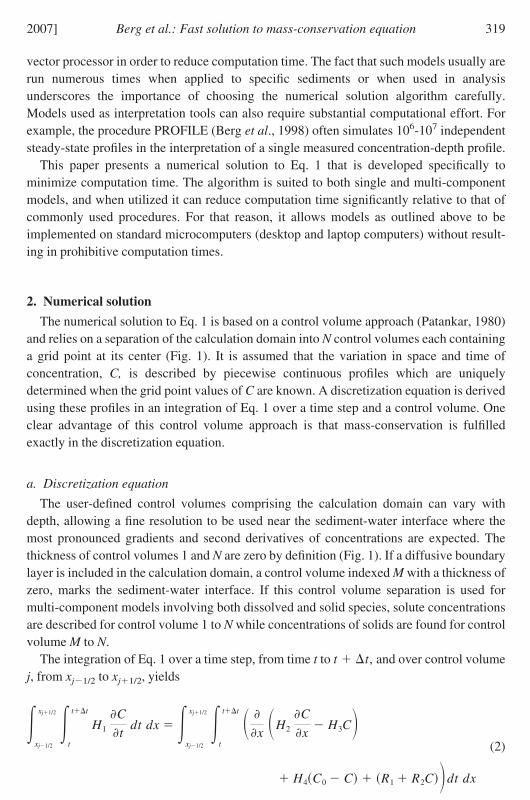

H1 jCjn1 Cj
n13xj t
t13t H2
C
x H3C
j12
H2
C
x H3C
j12
H4jC0 Cj R1 j R2 jCj13xjdt
(4)
where Cjn is the old (known) grid point value of C at time t and Cj
n1 is the new (unknown)grid point value of C at time t 13t
The second term on the right side of Eq 4 (H2C x H3C)j1 2 represents thecombined diffusive-advective flux Jj1 2 over the boundary between control volume j-1and j (Fig 1) It has long been known that a straightforward central difference approxima-tion of Jj1 2 inevitably leads to numerical instability when modeling advection-dominated systems (Courant et al 1952) For that reason researchers have suggestedapproximations of Jj1 2 that ensure unconditionally stable schemes (ie Courant et al1952 Spalding 1972 Fiadeiro and Veronis 1977 Patankar 1980 1981 Berg 1985)Some of the most successful schemes were derived as approximations to the analyticalsolution to the one-dimensional steady state mass-conservation equation accounting fortransport by diffusion and advection These schemes were defined through the 1970s andearly 1980s and their success was evaluated not only in terms of how well theyapproximated this analytical solution but also how fast they could be evaluated numeri-cally Because computer processors have changed radically since then the relative utility ofthese evaluation schemes have changed as well For this reason we compare theperformance of a selection of the most popular schemes on a modern microcomputer inAppendix A
Common to all these schemes is the expression of flux Jj1 2 as
Jj12 F1 jCj F2 jCj1 (5)
and the individual schemes are defined through their definition of F1 j and F2 j which arederived in details for these schemes in Appendix A Combining Eqs 4 and 5 gives
H1 jCjn1 Cj
n13xj t
t13t
F1 j1Cj1 F2 j1Cj F1 jCj F2 jCj1
H4jC0 Cj R1 j R2 jCj13xjdt
(6)
When approximating the time integral in Eq 6 it is necessary to assume how all thetime-dependent terms vary from time t to t 13t The time integral of Cj can be expressedas ((1 )Cj
n Cjn1)13t where is a weighting factor and different schemes will
result depending on the value of With 0 an explicit scheme is obtained while 1leads to an implicit scheme With 1frasl2 the Crank-Nicolson scheme a well-knownhybrid of the explicit and the implicit scheme is obtained The implicit scheme is chosenhere for the following reasons Firstly it leads to a versatile numerical solution allowing
2007] 321Berg et al Fast solution to mass-conservation equation
transient solutions to be found using appropriately sized time steps and at the same timeallowing steady-state solutions to linear problems to be produced with minimal computa-tional effort in one large time step Secondly the implicit scheme is especially attractive inone-dimensional formulations when computation time is of concern While the number ofnumeric operations per time step in the explicit Crank-Nicolson and implicit scheme issimilar a restrictive upper limit exists for the time steps in the explicit scheme Whenviolated numerical instability occurs For example in diffusion-dominated systems thiscritical time step equals 1
213x2H1H2 where H1 and H2 are given by Eq 3 In models of
organic matter and nutrient diagenesis where oxygen usually is a key component thattypically penetrates only a few mm into the sediments a 13x of 001 cm is required toaccurately describe the oxygen profile With typical values of H1 and H2 of 08 and105 cm2 s1 the critical time step is 4 s for the explicit scheme Such small time steps willlead to prohibitive computation times when multiple-year simulations are required Upperlimits to the time step obviously also exist for the implicit scheme in such simulations butthey are of a different nature and are generally markedly less restrictive For example inmulti-component models fast non-linear reactions between species can restrict the size ofthe time steps that can be used However in such modeling exercises performed withrealistic reaction rate constants time steps on the order of 1 h are usually sufficient toensure an accurate numerical solution as we demonstrate in an example below As theresult of the explicit element in the Crank-Nicolson scheme it can depending on theapplication also suffer from restrictive demands on the time step As a simple example ofthis it is not possible to produce steady-state solutions to linear problems in one large timestep as is the case with the implicit scheme
The implicit time integration in Eq 6 gives
H1 jCjn1 Cj
n13xj
13t F1 j1C j1
n1 F2 j1C jn1 F1 jC j
n1 F2 j C j1n1
H4jC0 C jn113xj R1 j R2 jC j
n113xj
(7)
which gives the following tri-diagonal system of equations
AAjCj1n1 BBjCj
n1 CCjCj1n1 DDj (8)
where the coefficients are defined as
AAj F2 j
BBj F1 j F2 j1 H4j13xj R2 j13xj H1 j
13xj
13t
CCj F1 j1
DDj H1 j
13xj
13tCj
n H4jC013xj R1 j13xj
(9)
322 [65 3Journal of Marine Research
The control volume spanning 13xj is included deliberately as a factor in Eq 9 rather than adenominator allowing 13xj to equal zero
b Boundary conditions
The boundary conditions that bring closure to the tri-diagonal system of equations(Eq 7) are imposed implicitly through control volume L and N where L equals either 1 orM depending on how the calculation domain is separated into control volumes (Fig 1) Forcontrol volume L and N Eq 8 simplifies to
BBLCLn1 CCLCL1
n1 DDL (10)
and
AANCN1n1 BBNCN
n1 DDN (11)
The coefficients BBL CCL DDL AAN BBN and DDN are given values depending on thekind of boundary conditions imposed Three types of boundary conditions are possible aknown concentration a known flux and a known concentration gradient The assignmentof values to BBL CCL DDL AAN BBN and DDN depending on the type and value of theboundary conditions are outlined in Table 1 The unique set of boundary concentrationsCL
n1 and CNn1 which ensures that the desired boundary conditions are imposed is
obtained when the tri-diagonal system of equations (Eqs 8 10 11) is solved
c Solution of tri-diagonal system of equations
Several models of biogeochemical transformations in aquatic sediments rely on implicitschemes In these models the tri-diagonal system of equations is typically solved byGaussian elimination numerous times in a single simulation (ie Dhakar and Burdige1996 Van Cappellen and Wang 1996) using for example the Thomas algorithm (iePatankar 1980 Huyakorn and Pinder 1983) Rather than performing this straightforward
Table 1 Definition of coefficients BBL CCL DDL AAN BBN and DDN in Eq 10 and 11 dependingon the imposed type and value of boundary condition
Upper boundary condition BBL CCL DDL
Known concentration 1 0 The known concentrationKnown flux F2L1 F1L1 The known fluxKnown gradient 213xL1 213xL1 The known gradient
Lower boundary condition AAN BBN DDN
Known concentration 0 1 The known concentrationKnown flux F2N F1N The known fluxKnown gradient 213xN1 213xN1 The known gradient
2007] 323Berg et al Fast solution to mass-conservation equation
Gaussian elimination in every time step a significant reduction in computation time can beobtained as follows
The coefficient DDj in the tri-diagonal system of equations (Eq 9 Table 1) willtypically vary from time step to time step in most applications simply because DDj
contains the concentration Cjn at the old time level t In contrast the coefficients AAj BBj
and CCj are likely to be constant throughout the simulation (Eq 9 Table 1) or at least varyat such a slow rate that it is appropriate to treat them as constants through manyconsecutive time steps An example of this is dynamic simulations based on time steps onthe order of minutes and where much slower seasonal temperature variations will affectvariables such as molecular diffusivities and thus AAj BBj and CCj In such simulationsit is clearly a good approximation only to update or recalculate the coefficients AAj BBj
and CCj on a weekly or monthly basis This characteristic can be taken advantage of toreduce the computational effort significantly in successive solutions of the tri-diagonalsystem of equations by decomposing the discretization matrix only once or only with timeintervals where AAj BBj and CCj vary markedly This is done by reformulating theThomas algorithm
The forward substitution in the Thomas algorithm where Eqs 8 10 and 11 are solved inthe interval L j N yields (ie Patankar 1980 Huyakorn and Pinder 1983)
PPL CCL
BBL QQL
DDL
BBL
PPj CCj
BBj AAjPPj1
QQj DDj AAjQQj1
BBj AAjPPj1
j L 1 3 N 1 (12)
QQN DDN AANQQN1
BBN AANPPN1
where PPj and QQj are decomposition variables and AAj BBj CCj and DDj are definedeither by Eq 9 or in Table 1 The following back substitution that gives the values of Cj
n1
yields
CNn1 QQN
(13)Cj
n1 PPjCj1n1 QQj j N 1 3 L
The significant gain in computational efficiency is now achieved by rewriting Eq 12 sothat DDj is kept out of the forward substitution by defining an additional decompositionvariable NNj as follows
324 [65 3Journal of Marine Research
NNL 1
BBL PPL CCLNNL
NNj 1
BBj AAjPPj1
PPj CCjNNj
j L 1 3 N 1 (14)
NNN 1
BBN AANPPN1
With this modification the back substitution that gives the values of Cjn1 then yields
QQL DDLNNL
QQj DDj AAjQQj1NNj j L 1 3 N(15)
CNn1 QQN
Cjn1 PPjCj1
n1 QQj j N 1 3 L
There are 5(N L) 1 numeric operations in Eq 15 approximately half the numberused in the original Thomas algorithm (10(N L) 1) Because multiplications arecomputationally less costly to perform than divisions the overall result is that Eq 15 are25 times faster to execute than those of the original Thomas algorithm on a 20 GHzPentium M PC
Another important and unique feature of this numerical solution is that the type ofboundary condition is introduced through BBL CCL AAN and BBN (Table 1) while thevalues of the boundary condition are imposed through DDL and DDN This characteristicallows the values of boundary conditions to vary as a simulation progresses withoutrequiring new decompositions of the discretization matrix
The coefficient DDj (Eq 9) must be calculated in every time step This is done mosteffectively as
DDj EEjCjn FFjC0 R1 j13xj (16)
where EEj and FFj are defined as
EEj H1 j
13xj
13tand FFj H4 j13xj (17)
which with the definitions of H1 j and H4 j (Eq 3) typically need only be evaluated onceIn summary it is convenient to calculate the coefficients given by Eqs 3 9 and 17 and
perform the new forward substitution given by Eq 14 in one algorithm We have namedthis algorithm CONSTANTS and its content is summarized in Appendix B The algorithmincludes five optional expressions for the molecular sediment diffusivity (Ds) as a functionof porosity and diffusivity in water The two first were originally defined by Ullman andAller (1982) the third and fourth were given by Iversen and Joslashrgensen (1993) and the fifth
2007] 325Berg et al Fast solution to mass-conservation equation
was defined by Boudreau (1997) The output from CONSTANTS are input to the secondalgorithm CNEW which performs the back substitution (Eq 15) leading to the newconcentrations every time it is utilized The content of CNEW is summarized in Appendix C
3 Applications and examples
The numerical solution separated into the two algorithms CONSTANTS and CNEW israther versatile and can be used to simulate steady state dynamic linear and nonlinearproblems that further can involve one or more dissolved or solid species The outlinedfeatures of the solution are particularly beneficial in applications where long computationtimes are of concern
Four example applications of the algorithm are presented below representing computa-tional gains achieved in diverse problems The first three focus on rather simple cases forwhich analytical solutions exist They also serve as a test of the numerical solution and asan illustration of the discretization in depth (and in time for transient problems) required toobtain accurate solutions In the last example the solution is implemented in a dynamicmulti-component and nonlinear model of organic matter and nutrient diagenesis in aspecific sediment This example illustrates clearly the significant advantages that can beachieved in terms of short computation times when applying the numerical solution tomodels where components with very different time constants require relatively small timesteps combined with long simulation times to produce quasi-stationary solution on a yearto year basis All examples are coded in FORTRAN 90 and the simulations are performedin double precision
a Example 1
Four types of solute transport molecular diffusion bioturbation irrigation and advec-tion are represented in Eq 1 An analytical solution to the equation is possible understeady-state conditions if advection and first-order production terms are neglected and if Ds DBw and R1 are assumed to be constant with depth Under these conditions Eq 1simplifies to
DBw Dsd2C
dx2 C0 C R1 0 (18)
which has the solution
C A exp
DBw Dsx B exp
DBw Dsx
C0 R1
(19)
where A and B are arbitrary constants (Boudreau 1997)Berg et al (1998) calculated a hypothetical O2 profile in the depth interval from 005
to 10 cm assuming constant consumption rates (R1) of 0004 and 0012 nmol cm3 s1 forthe depth intervals of 0 to 075 and 075 to 10 cm and then applying Eq 19 to each of these
326 [65 3Journal of Marine Research
intervals In the diffusive boundary layer (D) from 005 to 0 cm the solution simplifiesto a straight line It was further assumed that the O2 concentration equals 0 at 1 cm depthsand below Finally values of DBw Ds and of 075 3 106 cm2 s1 9 106 cm2
s1 and 5 106 s1 were assumed by Berg et al (1998) Here (Fig 2A) we extended thesolution to also include the depth interval of 1 to 125 cm for which Eq 18 simplifies to R1
C0The O2 profile was simulated repeatedly utilizing the algorithms CONSTANTS and
CNEW while the number of equally spaced control volumes (N) was increased incremen-tally The error of the numerical solution was determined as the maximum deviation in the005 to 125 cm depth interval from the analytical solution in percent of the water columnconcentration (Fig 2B) Since the numerical solution is fully implicit each simulatedsteady-state profile was determined in one single use of both CONSTANTS and CNEW inwhich an ldquoinfinitely largerdquo time step (1 1030 s) was specified The error of the numericalsolution declines rapidly with increasing N (Fig 2B) and errors 1 01 and 001 wasfound for N equal to 10 25 and 80 The local periodic variation of the error was caused byoffsets between the abrupt changes in the imposed O2 consumptions (Fig 2A) and theboundaries between control volumes
b Example 2
Two types of solid transport bioturbation and advection are included in Eq 1 Ananalytical solution to the equation is possible under steady-state conditions if zero order
Figure 2 (A) Hypothetical steady state O2 depth-profile defined analytically (dots) and simulatednumerically by utilizing the algorithms CONSTANTS and CNEW (line) The imposed O2
consumption varies with depth (step function) (B) The error of the numerical solution for differentnumbers of equally spaced control volumes separating the -005 to 125 cm depth interval
2007] 327Berg et al Fast solution to mass-conservation equation
production terms are neglected and if is assumed to be constant with depth Under theseconditions Eq 1 simplifies to
d
dx DBs
dC
dx wdC
dx
R2
s1 C 0 (20)
This equation describes for example a radioactive tracer such as 210Pb that is supplied to asediment surface at a constant rate is transported to deeper sediment layers and isdisappearing through a first order decay In this case the decay constant equalsR2s(1 ) Swaney (1999) showed that if DBs exhibits a parabolic decrease withdepth as DBs DBs0 (1 xL)2 the analytical solution to Eq 20 in the 0 to L depth intervalis
C C0 L
L xexp1
2Pe
x
L xK1
2Pe
L
L xK
12
Pe(21)
where C0 is the concentration at the sediment surface Pe is Peclet number equal towLDBs0 and K is the modified Bessel function of the order and of the second kind
where L2DBs0 14 With values of L DBs0 w and of 10 cm 005 cm2
year1 005 cm year1 and 00315 year1 a hypothetical 210Pb profile was calculatedfrom Eq 21 (Fig 3A) As in Example 1 the 210Pb profile was simulated repeatedly for
Figure 3 (A) Hypothetical steady state 210Pb depth-profile defined analytically (dots) and simulatednumerically by utilizing the algorithms CONSTANTS and CNEW (line) (B) The error of thenumerical solution for different numbers of equally spaced control volumes separating the 0 to 10cm depth interval
328 [65 3Journal of Marine Research
increasing N and the error of the numerical solution was determined as the maximumdeviation in the 0 to 10 cm depth interval from the analytical solution in percent of thesediment surface concentration (Fig 3B) Also in this example each numerical solutionwas found in one ldquoinfinitely largerdquo time step (1 1030 s) The error of the numericalsolution decreases with increasing N (Fig 3B) but not as pronounced as in Example 1Errors of 1 and 01 were found for N equal to 31 and 105
c Example 3
As an example of nonsteady-state conditions a conservative dissolved tracer that issupplied to a sediment from the overlying water is considered An analytical solution toEq 1 is possible if irrigation is neglected and it is assumed that Ds and DBw are constantwith depth Under these conditions Eq 1 simplifies to
C
t DBw Ds
2C
dx2 udC
dx(22)
If the diffusive boundary layer is neglected and the tracer is absent in the sediment at timezero after which the tracer concentration is increased momentarily to a constant value at thesediment surface the analytical solution to Eq 22 is
C 12
C0erfc x ut
2DBw Dst exp xu
DBw Ds erfc x ut
2DBw Dst (23)
where C0 is the tracer concentration at the sediment surface (Bear and Verruijt 1987)From Eq 23 two hypothetical profiles were calculated one where advection was neglectedand one where advection was included with a downward directed velocity of 5 cm day-1
(Fig 4A) Both profiles are valid for a time of 1 day after the water column concentrationwas increased and based on identical values of Ds and DBw of 5 106 cm2 s1 Each ofthe profiles were simulated repeatedly over a range of N and time steps (13t) The error ofthe numerical solution was determined as the maximum deviation in the 0 to 10 cm depthinterval from the analytical solution is a percent of the concentration on the sedimentsurface (Figs 4B and 4C) The error of the numerical solution decreases as expected withincreasing N and 13t As a result of numerical diffusion (ie Patankar 1980) the error isapproximately 10-fold larger for the profile influenced by advection This example showsthat transient simulations of advection-dominated systems demands relatively high num-bers of control volumes to obtain an accurate numerical solution
d Example 4
As a more realistic example from a modeling point of view the numerical solution wasimplemented in a simplified version of the dynamic diagenetic model put forward bySoetaert et al (1996) The simplification consists of neglecting the nitrogen cycling Thisleaves three reactions to be simulated (Table 2) oxic mineralization anoxic mineraliza-tion and oxidation of so-called reduced compounds such as NH4
Mn2 Fe2 and H2S
2007] 329Berg et al Fast solution to mass-conservation equation
which was modeled as one component and referred to as ODU (Oxygen DemandingUnits) In addition to ODU the model included O2 plus a rapidly and a slowly decompos-ing pool of organic matter (OM) Furthermore the active transport processes accounted forwere molecular diffusion bioturbation and burial as in the original model (Soetaert et al1996) The regulation of all reactions was adopted from Berg et al (2003) (Table 2) Themodel was applied to the Arctic sediment of one of the sites in Young Sound Greenlandmonitored intensively by Rysgaard and Berg (1996) and Rysgaard et al (1998) through afull annual cycle The site is located at 36 m depth has a constant temperature year roundand a supply of OM that follows a dynamic pattern strongly affected by a short ice-freeperiod in mid-summer
As a realistic test example of the numerical solution the model contains several ratherchallenging elements For example the reaction regulations are all clearly nonlinear andresult in nonlinear production terms (Table 2) These production terms couple the massconservation equations for the four simulated components making all four equationsnonlinear In addition both the depth and temporal scales of these components aremarkedly different Specifically O2 penetrates only a few mm into the sediment andadjusts to dynamic changes on a time scale of 10 to 100 min while decomposing OMreaches much larger sediment depths and adjusts to changes on a time scale of 10 to 100years
The numerical solution was implemented as follows As an initial step coefficients inthe systems of equations one system for each simulated component were evaluated andthe systems of equations were decomposed by the algorithm CONSTANTS utilized only
Figure 4 (A) Hypothetical transient depth-profiles after a one-day intrusion of a conservativedissolved tracer defined analytically (dots) and simulated numerically by utilizing the algorithmsCONSTANTS and CNEW (lines) The upper profile is influenced by diffusion only while thelower profile is the combined result of both diffusion and advection (B) Iso-plot of errors for thenumerically predicted diffusion controlled profile for different numbers of equally spaced controlvolumes separating the 0 to 10 cm depth interval and different time steps (C) Iso-plot of errors forthe numerically predicted diffusion and advection controlled profile for different numbers ofequally spaced control volumes separating the 0 to 10 cm depth interval and different time stepsNote that errors are approximately 10 times larger for the profile under influence of both diffusionand advection
330 [65 3Journal of Marine Research
once for each component In each of the following time steps first the reaction rates (V1f V1s V2f V2s V3) and then the production terms (ROMf ROMs RO2 RODU) were determinedfrom known concentrations at time t (Table 2) Based on these production terms newconcentrations for time t 13t were determined by the algorithm CNEW utilized once foreach component in every time step
This scheme relies on an explicit coupling between the mass balances through theproduction terms (ROMf ROMs RO2 RODU) In order to avoid instabilities arising fromthis explicit coupling especially in the initial phase of a simulation none of thereaction rates were allowed to be negative This was achieved by applying the intrinsicfunction MAX(a b) which returns the maximum value of arguments a and b
Site-specific quantities measured by Rysgaard and Berg (1996) Rysgaard et al (1998)
Table 2 Simplified diagenetic reactions their regulations and the constituents included in Example4 Simulated constituents are written in bold in the reactions The symbols OM and ODU are usedfor organic matter and oxygen demanding units A rapidly and a slowly decaying pool are utilizedfor OM
Reaction 1 OMf O2OiexclV1f
CO2 1
C NNH4
OMs O2OiexclV1s
CO2 1
C NNH4
Reaction 2 OMf an oxidantOiexclV2f
CO2 1
C NNH4
ODU
OMs an oxidantOiexclV2s
CO2 1
C NNH4
ODU
Reaction 3 ODU O2OiexclV3
an oxidant
RegulationsVf KOMf(1 )s[OMf] and Vs KOMs(1 )s[OMs]
O2 [O2lim] V1f Vf and V2f 0V1s Vs and V2s 0
O2 O2lim V1f Vf O2O2lim and V2f Vf V1f
V1s VsO2O2lim and V2s Vs V1s
V3 K3[ODU][O2]Production terms
ROMf V1f V2f and ROMs V1s V2s
RO2 V1f V1s V3
RODU V2f V2s V3
2007] 331Berg et al Fast solution to mass-conservation equation
and Berg et al (2001) were used for many input parameters to the model (1 2 3 6 7 8 910 11 Table 3) The limiting O2 concentration (12 Table 3) used in the regulation of thereactions was taken from Van Cappellen and Wang (1996) and Berg et al (2003) as wasthe rate constant for Reaction 3 (15 Table 3) This rate constant was used in these studiesfor the reaction of Fe2 with O2 and by adopting this constant here it was implicitlyassumed that the ODU pool consists mostly of Fe2 in accordance with the findings ofBerg et al (2003) at this site The distribution of the OM supply between the rapidly andthe slowly decomposing OM pools (16 Table 3) was taken from Soetaert et al (1996) Allthese parameters were kept constant in all simulations
The last three input parameters to be assigned the rate constants for the two OM poolsand the time dependant OM flux supplied to the sediment were given values by comparingsimulated and measured results repetitively and adjusting the three input parameters Basedon the measured pattern of O2 fluxes (Fig 5B) and also two OM sedimentation rates(Fig 5A) reported by Rysgaard et al (1998) it was assumed that the variation of the OMflux over the year consists of a base contribution plus a short peak summer contributionwith a duration of 1 month (Fig 5A) With a known annual supply of OM to the sediment(9 Table 3) also reported by Rysgaard et al (1998) the dynamic OM flux was uniquelydefined by the ratio between the peak summer contribution and the base contribution (17Table 3)
Despite the simplicity of the model a good agreement was achieved for the O2 uptake
Table 3 Input parameters in Example 4 and their origin
Parameter Value Source
1 Sedimentation rate w 012 cm year1 1 22 Biodiffusivity for solutes x 4 cm DBw 46 106 cm2 s1 3 (2)
x 4 cm DBw 46 106 e035(x4) cm2 s1
3 Biodiffusivity for solids DBs DBw12 3 (2)4 Molecular diffusivity at 0 degC DO2 117 106 cm2 s1 45 Molecular diffusivity at 0 degC DODU 34 106 cm2 s1 56 Porosity 0631 0207 e102x 6 (2)7 Density of solid sediment s 241 g cm3 68 Diffusive boundary layer D 003 cm 6 (2)9 Boundary condition FOM 2300 mmol m2 year1 6
10 Boundary condition [O2]x003 389 M 611 Boundary condition [ODU]x003 0 M 212 Limiting concentration [O2]lim 20 M 7 (2)13 Rate constant KOMf 20 106 s1 14 Rate constant KOMs 30 109 s1 15 Rate constant K3 11 106 M1 s1 7 (2)16 Ratio FOMf FOMs 05 817 Ratio FOM peakFOM base 6
1) Rysgaard et al (1996) 2) Berg et al (2003) 3) Berg et al (2001) 4) Broecker and Peng (1974) 5)Li and Gregory (1974) 6) Rysgaard et al (1998) 7) Van Cappellen and Wang (1996) 8) Soetaert etal (1996) This study
332 [65 3Journal of Marine Research
throughout the year (Fig 5B) A similarly good agreement was obtained with the measuredO2 concentration profile determined by Rysgaard et al (1998) in mid August (Fig 5C)
All simulations were based on a time step of 1 hour and a separation of the diffusiveboundary layer and the upper 20 cm of the sediment into 100 control volumes This depthwas required to diminish the slow pool of OM to close to zero concentrations (Fig 5D)The upper 1 cm of the sediment was separated into equally sized control volumes of 003cm after which the control volume size was gradually increased with depth Thisdiscretization in time and space was found to be adequate to obtain precise numericalsolutions in an additional simulation performed with a time step of 15 min and 200 controlvolumes which gave the same annual O2 uptake within 004
From initial conditions of zero OM O2 and ODU in the sediment 75 years of simulated
Figure 5 Application of a dynamic multi-component and nonlinear model of organic matter andnutrient diagenesis to an Arctic sediment (Table 2 and 3) by utilizing the algorithms CONSTANTSand CNEW (A) Supply of organic matter to the sediment over the year found in the modelparameterization (line) and two measured organic matter fluxes (dots) (B) Simulated (line) andmeasured (bars errors represent 1 SE n 6) O2 uptake over the year (C) Simulated (line) andmeasured (dots) O2 depth-profile in mid August (D) Simulated depth-profile of decomposingorganic matter (E) Simulated depth-integrated organic matter content through 75 years ofsimulated time Initial condition in the simulation was a sediment absent of organic matter (F)Computation time required per simulated year using the standard Thomas algorithm as equationsolver and the algorithm presented in this study The results were produced on a 20 GHz PentiumM PC
2007] 333Berg et al Fast solution to mass-conservation equation
time were required to build up the OM pools to quasi-stationary conditions on a year toyear basis (Fig 5E) Even though some 50 simulations were performed in this modelparameterization the 75 years of simulated time did not lead to prohibitive computationtimes as the model was running at the speed of 013 s per simulated year on a 20 GHzPentium M PC (Fig 5F) This good performance was the combined result of three factorsFirstly the implicit formulation in the numerical solution allowed a relatively large timestep to be used Specifically the time step was 100 times larger than the maximum allowedcritical time step of explicit formulations (see above) Secondly the separation of theforward and the back substitution in the numerical solution allowed the system of 100equations per simulated component to be decomposed only once after which newconcentrations were found with little computational effort in every time step Thirdly thenovel implementation of boundary conditions allowed the values of boundary conditions tovary as simulations progressed without requiring new decompositions of the systems ofequations This characteristic was clearly taken advantage of here with respect to theimposed OM flux (Fig 5A) An additional simulation performed with the standardThomas algorithm as equation solver (Eqs 12 and 13) instead of our algorithms (Eqs 14and 15) required the double amount of computation time (Fig 5F) It should beemphasized that this simulation with the standard Thomas algorithm also was optimizedwith respect to computation time by only calculating the constants AAj BBj and CCj (Eq9) once Because the number of numeric operations in multi-component diagenetic modelstypically varies linearly with the number of species accounted for this factor of twoconservatively represents the computational efficiency to be gained over the Thomasalgorithm by using the algorithms proposed in this study
The explicit coupling used between the mass balances for each component represents thesimplest possible way to overcome the inherent nonlinearities in multi-component diage-netic models A more advanced implicit coupling that would allow markedly larger timesteps than used here is also possible Although this would require iterations to beperformed in every time step to overcome these nonlinearities it would lead to even fasteroverall computation times In such formulations the algorithms CONSTANTS and CNEWcan also be used equally as effectively Details on how to formulate such iterative schemesmost effectively are for example given by Patankar (1980) and Berg (1999)
4 Summary and conclusion
Many researchers modeling species transformations in aquatic sediments have foundthat computation times of numerical solutions can become prohibitively long In manycases this is either due to inefficient algorithms or to algorithms being misapplied toproblems inappropriate to them The numerical solution presented here is suited to bothsingle and multi-component models and aims to minimize this problem taking advantageof three factors
1 The numerical solution is based on an implicit formulation of the discretizationequation which provides a versatile approach for solving transient problems using
334 [65 3Journal of Marine Research
relatively large time steps and at the same time allowing steady-state solutions tolinear problems to be produced in one single ldquoinfinitely largerdquo time step
2 Care has been taken to re-calculate model variables only when necessary ie as asimulation progresses when or if they change For example in transient solutions allnon-essential numerical operations are eliminated from the repetitive time loopConsequently the numerical solution consists of two algorithms CONSTANTS andCNEW one that decomposes the discretization matrix once and one that subse-quently can be utilized numerous times with minimal computational effort Intransient solutions this will be in every time step
3 The algorithms are uniquely formulated to allow the values of boundary conditions tovary as a simulation progresses without requiring new decompositions of thediscretization matrix
The combined effect of these features can reduce computation times significantlyrelative to procedures commonly used for modeling species transformations in aquaticsediments Although the last example presented above focuses on a relatively simplediagenetic model it illustrates clearly the potential benefits in terms of computation timesthat can be achieved with this numerical solution
Available Software
Copies of the algorithms CONSTANTS and CNEW coded in FORTRAN 90 can beobtained free of charge from the corresponding author For optimal performance thealgorithms should be applied in double precision
Acknowledgments We thank D Burdige and one anonymous reviewer for their constructivereviews of this paper This study was supported by grants from the University of Virginia and theDanish National Science Research Councils (contract nos 9501025 and 9700224)
APPENDIX A
Approximation of fluxes
As illustrated by Patankar (1980) a first evaluation of flux-approximating schemes canbe achieved by comparison with the analytical solution of the one-dimensional steady statemass-conservation equation that accounts for diffusion and advection This approach isadapted here and complemented with computation times for evaluation of the schemes onmodern computer processors The one-dimensional steady state mass-conservation equa-tion including diffusive and advective transport contributions can be written in the form
dJ
dx 0
(A1)
J H2
dC
dx H3C
2007] 335Berg et al Fast solution to mass-conservation equation
If H2 and H3 are constant with depth Eq A1 have the analytical solution (ie Patankar1980 or Boudreau 1997)
x 0 C C0
x L C CL f J H3C0
C0 CL
expH3
H2L 1 (A2)
Assuming for now that 13xj is constant with depth and referred to as 13x and using thissolution to express the intermediate combined diffusive-advective flux Jj1 2 at theboundary between control volume j-1 and j gives
Jj12 H3Cj1 FPCj1 Cj
P (A3)
where the function F(P) is given by
FP P
expP 1(A4)
and where P is the Peclet number defined as
P H3
H213x (A5)
Numerical solutions of Eq 1 can be produced by expressing the fluxes between controlvolumes according to Eq A3 The expression of Jj1 2 in combination with Eq A4 isoften referred to as the exponential scheme based on the expression for F(P) and was firstput forward by Spalding (1972) and later by Fiadeiro and Veronis (1977) At the time whenthe exponential scheme was defined the exponential function was time consuming toevaluate on computers of the day In addition F(P) needs special attention in its evaluationas it contains a singularity for P 0 For those reasons researchers derived new schemesrelying on approximations of F(P) that were markedly faster to evaluate (ie Spalding1972 Patankar 1981 Berg 1985) The most popular schemes including the classiccentral difference and upwind schemes (Courant et al 1952) are shown in Table A1 alongwith the normalized computation time for their evaluation on a 20 GHz Pentium M PC Asan example of derivation the central difference approximation of F(P) can be derived byapproximating the intermediate flux as Jj1 2 H2(Cj Cj1)13x H3(Cj Cj1) 2 which is equivalent to Eq A3 if F(P) 1 05P (Table A1) The exactfunction F(P) and its approximations are illustrated in Figure A1
The central difference scheme provides a good approximation of F(P) only for smallvalues of P and is the only scheme in which the divergence from F(P) 3 as P 3 (Fig 1A) This characteristic explains why instabilities occur when using central differ-ence approximation for advection-dominated systems (P 0) The normalizedcomputation times (Table A1) show that the power law scheme which was used exten-sively in the 1980s and 1990s is outdated today as its evaluation is more time consuming
336 [65 3Journal of Marine Research
than the exact scheme Both the hyperbolic and the hybrid scheme appear to be goodchoices based on their good approximation of F(P) (Fig A1) in combination with theirrelatively short evaluation times However it should be noted that the evaluation time
Table A1 Formulations of the function F(P) in different schemes The formulations are given on aform that ensures minimal use of computation time in their evaluations The normalized evaluationtimes are valid for a 20 GHz Pentium M PC The two intrinsic functions SIGN and MAX eachhave two arguments and are standard functions in FORTRAN Function SIGN performs a signtransfer by returning the absolute value of the first argument multiplied by the sign of the secondargument Function MAX returns the maximum value of the arguments
Scheme Approximations of F(P) P(exp(P) 1)Normalized time
for one evaluation Reference
Exact Phelp SIGN(MAX(105 P) P)F(P) Phelp(exp(Phelp) 1) 10 1) 2)
Power law F(P) MAX(0 (1 01P)5) MAX(0 P) 12 3)Hyperbolic F(P) MAX(0 8(4 P) 1) MAX(0 P) 0093 4)Hybrid F(P) MAX(0 P 1 05P) 0062 1)Upwind F(P) MAX(1 1 P) 0047 5)Central F(P) 1 05P 0037
1) Spalding 1972 2) Fiadeiro and Veronis 1977 3) Patankar 1981 4) Berg 1985 5) Courant et al1952
Figure A1 The exact function F(P) and its approximation in alternate schemes
2007] 337Berg et al Fast solution to mass-conservation equation
should affect the choice of scheme only in model formulations where numerous evalua-tions of F(P) are expected
In this brief comparison it was assumed that 13x H2 and H3 are constant with depthThis is only true for H3 in Eq 3 and an expression similar to Eq A3 where variations in 13xand H2 are accounted for is derived from Eq A2 as follows Assuming that the grid pointvalues of H2 prevail throughout control volumes as representative mean values the fluxJj1 2 can be expressed for control volume j-1 by the variables Cj1 Cj1 2 13xj1H2 j1 and H3 as
Jj12 H3Cj1 Cj1 Cj12
exp H3
H2 j1
1
213xj1 1 (A6)
The same flux can similarly be expressed for control volume j by the variables Cj1 2 Cj13xj H2 j and H3 as
Jj12 H3Cj12 Cj12 Cj
expH3
H2 j
1
213xj 1 (A7)
Eliminating Cj1 2 by combining these two expressions leads to (equivalent to Eq A3)
Jj12 H3Cj1 FPj12Cj1 Cj
Pj12 (A8)
where the function F(Pj1 2) is given by (equivalent to Eq A4)
FPj12 Pj12
expPj12 1(A9)
and the Peclet number Pj1 2 is defined as the simple average of Pj1 and Pj (equivalent toEq A5)
Pj12 1
2 H313xj1
H2 j1
H313xj
H2 j (A10)
or alternatively as
Pj12 H3
H2 j12
12
13xj1 13xj (A11)
where H2 j1 2 is given by the weighted harmonic mean of H2 j1 and H2 j as
H2 j12 H2 j1H2 j13xj1 13xj
13xj1H2 j 13xjH2 j1(A12)
338 [65 3Journal of Marine Research
The general expression of the flux Jj1 2 over the boundary between control volume j-1and j is defined by the two variables F1 j and F2 j (Eq 5) These variables can now bederived from Eq A8 as
F1 j FPj12H2 j12
1213xj1 13xj (A13)
F2 j F1 j H3
where the function F(Pj1 2) is taken from Table A1
APPENDIX B
The algorithm ldquoCONSTANTSrdquo
Below is listed the input to and the output from the algorithm CONSTANTS followedby a summary of the algorithm Units of input and output variables are included as anexample Other units can be used as long as they are mutually consistent
Input
L [-] Number of first control volume (1 or M see Fig 1)M [-] Number of control volume at the sediment surface (see Fig 1)N [-] Number of last control volume (see Fig 1)13t [s] Time step13xj [cm] Size of control volumesj [-] PorosityD [cm2 s1] Diffusivity in waterDBw j [cm2 s1] Biodiffusivity for solutesDBs j [cm2 s1] Biodiffusivity for solidss [g cm3] Density of sedimentj [s1] Irrigation coefficientR2 j [s1] Production rates(u)x [m s1] Porosity times porewater velocity (constant with depth)((1 )w)x [m s1] One minus porosity times burial velocity (constant with depth) [-] Equal to 1 for solutes and equal to 0 for solids [cm3 g1] Coefficient (0 1 or K where K is the adsorption constant)FL0 [-] Flag for choosing the expression for Ds (1 2 3 4 or 5)FL1 [-] Flag for choosing the upper boundary condition (1 2 or 3)FL2 [-] Flag for choosing the lower boundary condition (1 2 or 3)
Output
AAj [cm s1] Input to CNEWEEj [cm s1] Input to CNEWFFj [cm s1] Input to CNEWNNj [s cm1] Input to CNEWPPj [-] Input to CNEWF1 j [cm s1] Constants for calculation of flux (Eq 5)F2 j [cm s1] Constants for calculation of flux (Eq 5)
Calculation of Dsj depending of the flag FL0
2007] 339Berg et al Fast solution to mass-conservation equation
FL0 1 Ds j jD
FL0 2 Ds j j2D
FL0 3 Ds j D
1 21 j
FL0 4 Ds j D
1 31 j
FL0 5 Ds j D
1 lnj2
j L 3 N (B1)
Calculation of H1j H2j H3 and H4j
H3 ux s1 wx
(B2)H1 j j s1 jH2 j jDBw j Ds j s1 jDBs jH4 j jj
j L 3 N
Calculation of F1 j and F2 j Note that special precautions are taken to avoid division byzero The function MAX(a b) is a standard function in FORTRAN and returns themaximum value in the argument list The number 1036 is close to the smallest value thatcan be represented in single precision in FORTRAN
H2 j12 H2 j1H2 j13xj1 13xj
MAX1036 13xj1H2 j 13xjH2 j1
Pj12 H3
MAX1036 H2 j121213xj1 13xj
FPj12 MAX0 84 Pj12 1 MAX0 Pj12
F1 j FPj12H2 j12
1213xj1 13xj
F2 j F1 j H3
j L 1 3 N (B3)
Calculation of the coefficients AAj BBj and CCj in the tri-diagonal system of equations
AAj F2 j
BBj F1 j F2 j1 H4 j13xj R2 j13xj H1 j
13xj
13t
CCj F1 j1
j L 1 3 N 1 (B4)
Calculation of the coefficients BBL and CCL for the upper boundary condition The type ofboundary condition is specified by the flag FL1
340 [65 3Journal of Marine Research
FL1 1 BBL 1 CCL 0
FL1 2 BBL F2 L1 CCL F1 L1 (B5)
FL1 3 BBL 2
13xL1 CCL BBL
Calculation of the coefficients AAN and BBN for the lower boundary condition The type ofboundary condition is specified by the flag FL2
FL2 1 AAN 0 BBN 1
FL2 2 AAN F2 N BBN F1 N (B6)
FL2 3 AAN 2
13xN1 BBN AAN
Calculation of the coefficients NNj and PPj in the forward substitution
NNL 1
BBL PPL CCLNNL
NNj 1
BBj AAjPPj1
PPj CCjNNj j L 1 3 N 1 (B7)
NNN 1
BBN AANPPN1
Calculation of the coefficients EEj and FFj used to calculate the right hand side in thetri-diagonal system of equations
EEj H1 j
13xj
13t
FFj H4 j13xj j L 1 3 N 1 (B8)
APPENDIX C
The algorithm ldquoCNEWrdquo
Below is listed the input to and the output from the algorithm CNEW followed by asummary of the algorithm Units of input and output variables are included as an exampleOther units can be used as long as they are mutually consistent
Input
L [-] Number of first control volume (1 or M see Fig 1)N [-] Number of last control volume (see Fig 1)13xj [cm] Size of control volumesAAj [cm s1] Input from CONSTANTSEEj [cm s1] Input from CONSTANTSFFj [cm s1] Input from CONSTANTS
2007] 341Berg et al Fast solution to mass-conservation equation
Input (continued)
NNj [s cm1] Input from CONSTANTSPPj [-] Input from CONSTANTSC0 [nmol cm3] Known water column concentrationCj
n Solute [nmol cm3] Known concentrations at the old time levelSolid [nmol g1]
R1 j [nmol cm3 s1] Production ratesBCL FL1 1 [nmol cm3] or
[nmol g1]Known boundary condition at top
FL1 2 [nmol cm2 s1]FL1 3 [nmol cm4] or
[nmol g1 cm1]BCN FL2 1 [nmol cm3] or
[nmol g1]Known boundary condition at bottom
FL2 2 [nmol cm2 s1]FL2 3 [nmol cm4] or
[nmol g1 cm1]Output
Cjn1 Solute [nmol cm3] New concentrations at the new time level
Solid [nmol g1]
Calculation of the coefficients QQj
QQL BCLNNL
QQj EEjCjn FFjC0 R1 j13xj AAjQQj1NNj j L 1 3 N 1
(C1)
Calculation of the new concentrations Cjn1
CNn1 BCN AANQQN1NNN
Cjn1 PPjCj1
n1 QQj j N 1 3 L(C2)
REFERENCESBear J and A Verruijt 1987 Modeling Groundwater Flow and Pollution Theory and applications
of Transport in Porous Media Kluwer Academic Publisher Group 414 ppBerg P 1985 Discretization of the general transport equation presented in cylindrical coordinates in
Proceedings of the first Danish-Polish workshop on modeling heat flow and fluid flow problemsM Dytczak and P N Hansen eds Thermal Insulation Laboratory Technical University ofDenmark 95ndash105
mdashmdash 1999 Long-term simulation of water movement in soils using mass-conserving proceduresAdv Water Resources 22 419ndash430
Berg P N Risgaard-Petersen and S Rysgaard 1998 Interpretation of measured concentrationprofiles in sediment pore water Limnol Oceanogr 43 1500ndash1510
Berg P S Rysgaard P Funch and M K Sejr 2001 Effects of bioturbation on solutes and solids inmarine sediments Aq Micro Ecol 26 81ndash94
Berg P S Rysgaard and B Thamdrup 2003 Dynamic modeling of early diagenesis and nutrientcycling A case study in an Arctic marine sediment Amer J Sci 303 905ndash955
342 [65 3Journal of Marine Research
Berner R A 1980 Early Diagenesis A Theoretical approach Princeton University Press 241 ppBoudreau B P 1996 A method-of-lines code for carbon and nutrient diagenesis in aquatic
sediments CompGeosci 22 479ndash496mdashmdash 1997 Diagenetic Models and Their Implementation Springer-Verlag 414 ppBroecker W S and T-H Peng 1974 Gas exchange rates between air and sea Tellus 26 21ndash 35Courant R E Isaacson and M Rees 1952 On the solution of non-linear hyperbolic differential
equations by finite differences Comm Pure Appl Math 5 243ndash255Dhakar S P and D J Burdige 1996 A coupled non-linear steady state model for early diagenetic
processes in pelagic sediments Amer J Sci 296 296ndash330Fiadeiro M E and G Veronis 1977 On weighted-mean schemes for finite-difference approxima-
tion to the advection-diffusion equation Tellus 29 512ndash522Huyakorn P S and C F Pinder 1983 Computational Methods of Subsurface Flow Princeton
University Press 473 ppIversen N and B B Joslashrgensen 1993 Measurements of the diffusion coefficients in marine
sediments influence of porosity Geochim Cosmochim Acta 57 571ndash578Li Y-H and S Gregory 1974 Diffusion of ions in sea water and deep-sea sediments Geochim
Cosmochim Acta 38 703ndash714Luff R K Wallmann S Grandel and M Schluter 2000 Numerical modeling of benthic processes
in the deep Arabian Sea Deep-Sea Res II 47 3039ndash3072Meysman F J R J J Middelburg P M J Herman and C H R Heip 2003 Reactive transport in
surface sediments II Media an object-oriented problem-solving environment for early diagen-esis CompGeosci 29 301ndash318
Meile C C M Koretsky and P Van Cappellen 2001 Quantifying bioirrigation in aquaticsediments An inverse modeling approach Limnol Oceanogr 46 164ndash177
Mulsow S B P Boudreau and J N Smith 1998 Bioturbation and porosity gradients LimnolOceanogr 43 1ndash9
Patankar S V 1980 Numerical Heat Transfer and Fluid Flow McGraw Hill 197 ppmdashmdash 1981 Calculation procedure for two-dimensional elliptic situations Num Heat Transfer 4
409ndash425Rysgaard S and P Berg 1996 Mineralization in a northeastern Greenland sediment mathematical
modelling measured sediment pore water profiles and actual activities Aq Micro Ecol 11297ndash305
Rysgaard S B Thamdrup N Risgaard-Petersen H Fossing P Berg P B Christensen and TDalsgaard 1998 Seasonal carbon and nitrogen mineralization in a high-Arctic coastal marinesediment Young Sound Northeast Greenland Mar Ecol Prog Ser 175 261ndash276
Soetaert K P M J Herman and J J Middelburg 1996 A model of early diagenetic processes fromthe shelf to abyssal depths Geochim Cosmochim Acta 60 1019ndash1040
Spalding D B 1972 A novel finite-difference formulation for differential expression involving bothfirst and second derivatives Inter J Num Methods England 4 551ndash559
Swaney D P 1999 Analytical solution of Boudreaursquos equation for a tracer subject to food-feedbackbioturbation Limnol Oceanogr 44 697ndash698
Ullman W J and R C Aller 1982 Diffusion coefficients in nearshore marine sediments LimnolOceanogr 27 552ndash556
Van Cappellen P and Y Wang 1996 Cycling of iron and manganese in surface sediments Ageneral theory for the coupled transport and reaction of carbon oxygen nitrogen sulfur iron andmanganese Amer J Sci 296 197ndash243
Received 12 December 2006 revised 27 February 2007
2007] 343Berg et al Fast solution to mass-conservation equation

NNL 1
BBL PPL CCLNNL
NNj 1
BBj AAjPPj1
PPj CCjNNj
j L 1 3 N 1 (14)
NNN 1
BBN AANPPN1
With this modification the back substitution that gives the values of Cjn1 then yields
QQL DDLNNL
QQj DDj AAjQQj1NNj j L 1 3 N(15)
CNn1 QQN
Cjn1 PPjCj1
n1 QQj j N 1 3 L
There are 5(N L) 1 numeric operations in Eq 15 approximately half the numberused in the original Thomas algorithm (10(N L) 1) Because multiplications arecomputationally less costly to perform than divisions the overall result is that Eq 15 are25 times faster to execute than those of the original Thomas algorithm on a 20 GHzPentium M PC
Another important and unique feature of this numerical solution is that the type ofboundary condition is introduced through BBL CCL AAN and BBN (Table 1) while thevalues of the boundary condition are imposed through DDL and DDN This characteristicallows the values of boundary conditions to vary as a simulation progresses withoutrequiring new decompositions of the discretization matrix
The coefficient DDj (Eq 9) must be calculated in every time step This is done mosteffectively as
DDj EEjCjn FFjC0 R1 j13xj (16)
where EEj and FFj are defined as
EEj H1 j
13xj
13tand FFj H4 j13xj (17)
which with the definitions of H1 j and H4 j (Eq 3) typically need only be evaluated onceIn summary it is convenient to calculate the coefficients given by Eqs 3 9 and 17 and
perform the new forward substitution given by Eq 14 in one algorithm We have namedthis algorithm CONSTANTS and its content is summarized in Appendix B The algorithmincludes five optional expressions for the molecular sediment diffusivity (Ds) as a functionof porosity and diffusivity in water The two first were originally defined by Ullman andAller (1982) the third and fourth were given by Iversen and Joslashrgensen (1993) and the fifth
2007] 325Berg et al Fast solution to mass-conservation equation
was defined by Boudreau (1997) The output from CONSTANTS are input to the secondalgorithm CNEW which performs the back substitution (Eq 15) leading to the newconcentrations every time it is utilized The content of CNEW is summarized in Appendix C
3 Applications and examples
The numerical solution separated into the two algorithms CONSTANTS and CNEW israther versatile and can be used to simulate steady state dynamic linear and nonlinearproblems that further can involve one or more dissolved or solid species The outlinedfeatures of the solution are particularly beneficial in applications where long computationtimes are of concern
Four example applications of the algorithm are presented below representing computa-tional gains achieved in diverse problems The first three focus on rather simple cases forwhich analytical solutions exist They also serve as a test of the numerical solution and asan illustration of the discretization in depth (and in time for transient problems) required toobtain accurate solutions In the last example the solution is implemented in a dynamicmulti-component and nonlinear model of organic matter and nutrient diagenesis in aspecific sediment This example illustrates clearly the significant advantages that can beachieved in terms of short computation times when applying the numerical solution tomodels where components with very different time constants require relatively small timesteps combined with long simulation times to produce quasi-stationary solution on a yearto year basis All examples are coded in FORTRAN 90 and the simulations are performedin double precision
a Example 1
Four types of solute transport molecular diffusion bioturbation irrigation and advec-tion are represented in Eq 1 An analytical solution to the equation is possible understeady-state conditions if advection and first-order production terms are neglected and if Ds DBw and R1 are assumed to be constant with depth Under these conditions Eq 1simplifies to
DBw Dsd2C
dx2 C0 C R1 0 (18)
which has the solution
C A exp
DBw Dsx B exp
DBw Dsx
C0 R1
(19)
where A and B are arbitrary constants (Boudreau 1997)Berg et al (1998) calculated a hypothetical O2 profile in the depth interval from 005
to 10 cm assuming constant consumption rates (R1) of 0004 and 0012 nmol cm3 s1 forthe depth intervals of 0 to 075 and 075 to 10 cm and then applying Eq 19 to each of these
326 [65 3Journal of Marine Research
intervals In the diffusive boundary layer (D) from 005 to 0 cm the solution simplifiesto a straight line It was further assumed that the O2 concentration equals 0 at 1 cm depthsand below Finally values of DBw Ds and of 075 3 106 cm2 s1 9 106 cm2
s1 and 5 106 s1 were assumed by Berg et al (1998) Here (Fig 2A) we extended thesolution to also include the depth interval of 1 to 125 cm for which Eq 18 simplifies to R1
C0The O2 profile was simulated repeatedly utilizing the algorithms CONSTANTS and
CNEW while the number of equally spaced control volumes (N) was increased incremen-tally The error of the numerical solution was determined as the maximum deviation in the005 to 125 cm depth interval from the analytical solution in percent of the water columnconcentration (Fig 2B) Since the numerical solution is fully implicit each simulatedsteady-state profile was determined in one single use of both CONSTANTS and CNEW inwhich an ldquoinfinitely largerdquo time step (1 1030 s) was specified The error of the numericalsolution declines rapidly with increasing N (Fig 2B) and errors 1 01 and 001 wasfound for N equal to 10 25 and 80 The local periodic variation of the error was caused byoffsets between the abrupt changes in the imposed O2 consumptions (Fig 2A) and theboundaries between control volumes
b Example 2
Two types of solid transport bioturbation and advection are included in Eq 1 Ananalytical solution to the equation is possible under steady-state conditions if zero order
Figure 2 (A) Hypothetical steady state O2 depth-profile defined analytically (dots) and simulatednumerically by utilizing the algorithms CONSTANTS and CNEW (line) The imposed O2
consumption varies with depth (step function) (B) The error of the numerical solution for differentnumbers of equally spaced control volumes separating the -005 to 125 cm depth interval
2007] 327Berg et al Fast solution to mass-conservation equation
production terms are neglected and if is assumed to be constant with depth Under theseconditions Eq 1 simplifies to
d
dx DBs
dC
dx wdC
dx
R2
s1 C 0 (20)
This equation describes for example a radioactive tracer such as 210Pb that is supplied to asediment surface at a constant rate is transported to deeper sediment layers and isdisappearing through a first order decay In this case the decay constant equalsR2s(1 ) Swaney (1999) showed that if DBs exhibits a parabolic decrease withdepth as DBs DBs0 (1 xL)2 the analytical solution to Eq 20 in the 0 to L depth intervalis
C C0 L
L xexp1
2Pe
x
L xK1
2Pe
L
L xK
12
Pe(21)
where C0 is the concentration at the sediment surface Pe is Peclet number equal towLDBs0 and K is the modified Bessel function of the order and of the second kind
where L2DBs0 14 With values of L DBs0 w and of 10 cm 005 cm2
year1 005 cm year1 and 00315 year1 a hypothetical 210Pb profile was calculatedfrom Eq 21 (Fig 3A) As in Example 1 the 210Pb profile was simulated repeatedly for
Figure 3 (A) Hypothetical steady state 210Pb depth-profile defined analytically (dots) and simulatednumerically by utilizing the algorithms CONSTANTS and CNEW (line) (B) The error of thenumerical solution for different numbers of equally spaced control volumes separating the 0 to 10cm depth interval
328 [65 3Journal of Marine Research
increasing N and the error of the numerical solution was determined as the maximumdeviation in the 0 to 10 cm depth interval from the analytical solution in percent of thesediment surface concentration (Fig 3B) Also in this example each numerical solutionwas found in one ldquoinfinitely largerdquo time step (1 1030 s) The error of the numericalsolution decreases with increasing N (Fig 3B) but not as pronounced as in Example 1Errors of 1 and 01 were found for N equal to 31 and 105
c Example 3
As an example of nonsteady-state conditions a conservative dissolved tracer that issupplied to a sediment from the overlying water is considered An analytical solution toEq 1 is possible if irrigation is neglected and it is assumed that Ds and DBw are constantwith depth Under these conditions Eq 1 simplifies to
C
t DBw Ds
2C
dx2 udC
dx(22)
If the diffusive boundary layer is neglected and the tracer is absent in the sediment at timezero after which the tracer concentration is increased momentarily to a constant value at thesediment surface the analytical solution to Eq 22 is
C 12
C0erfc x ut
2DBw Dst exp xu
DBw Ds erfc x ut
2DBw Dst (23)
where C0 is the tracer concentration at the sediment surface (Bear and Verruijt 1987)From Eq 23 two hypothetical profiles were calculated one where advection was neglectedand one where advection was included with a downward directed velocity of 5 cm day-1
(Fig 4A) Both profiles are valid for a time of 1 day after the water column concentrationwas increased and based on identical values of Ds and DBw of 5 106 cm2 s1 Each ofthe profiles were simulated repeatedly over a range of N and time steps (13t) The error ofthe numerical solution was determined as the maximum deviation in the 0 to 10 cm depthinterval from the analytical solution is a percent of the concentration on the sedimentsurface (Figs 4B and 4C) The error of the numerical solution decreases as expected withincreasing N and 13t As a result of numerical diffusion (ie Patankar 1980) the error isapproximately 10-fold larger for the profile influenced by advection This example showsthat transient simulations of advection-dominated systems demands relatively high num-bers of control volumes to obtain an accurate numerical solution
d Example 4
As a more realistic example from a modeling point of view the numerical solution wasimplemented in a simplified version of the dynamic diagenetic model put forward bySoetaert et al (1996) The simplification consists of neglecting the nitrogen cycling Thisleaves three reactions to be simulated (Table 2) oxic mineralization anoxic mineraliza-tion and oxidation of so-called reduced compounds such as NH4
Mn2 Fe2 and H2S
2007] 329Berg et al Fast solution to mass-conservation equation
which was modeled as one component and referred to as ODU (Oxygen DemandingUnits) In addition to ODU the model included O2 plus a rapidly and a slowly decompos-ing pool of organic matter (OM) Furthermore the active transport processes accounted forwere molecular diffusion bioturbation and burial as in the original model (Soetaert et al1996) The regulation of all reactions was adopted from Berg et al (2003) (Table 2) Themodel was applied to the Arctic sediment of one of the sites in Young Sound Greenlandmonitored intensively by Rysgaard and Berg (1996) and Rysgaard et al (1998) through afull annual cycle The site is located at 36 m depth has a constant temperature year roundand a supply of OM that follows a dynamic pattern strongly affected by a short ice-freeperiod in mid-summer
As a realistic test example of the numerical solution the model contains several ratherchallenging elements For example the reaction regulations are all clearly nonlinear andresult in nonlinear production terms (Table 2) These production terms couple the massconservation equations for the four simulated components making all four equationsnonlinear In addition both the depth and temporal scales of these components aremarkedly different Specifically O2 penetrates only a few mm into the sediment andadjusts to dynamic changes on a time scale of 10 to 100 min while decomposing OMreaches much larger sediment depths and adjusts to changes on a time scale of 10 to 100years
The numerical solution was implemented as follows As an initial step coefficients inthe systems of equations one system for each simulated component were evaluated andthe systems of equations were decomposed by the algorithm CONSTANTS utilized only
Figure 4 (A) Hypothetical transient depth-profiles after a one-day intrusion of a conservativedissolved tracer defined analytically (dots) and simulated numerically by utilizing the algorithmsCONSTANTS and CNEW (lines) The upper profile is influenced by diffusion only while thelower profile is the combined result of both diffusion and advection (B) Iso-plot of errors for thenumerically predicted diffusion controlled profile for different numbers of equally spaced controlvolumes separating the 0 to 10 cm depth interval and different time steps (C) Iso-plot of errors forthe numerically predicted diffusion and advection controlled profile for different numbers ofequally spaced control volumes separating the 0 to 10 cm depth interval and different time stepsNote that errors are approximately 10 times larger for the profile under influence of both diffusionand advection
330 [65 3Journal of Marine Research
once for each component In each of the following time steps first the reaction rates (V1f V1s V2f V2s V3) and then the production terms (ROMf ROMs RO2 RODU) were determinedfrom known concentrations at time t (Table 2) Based on these production terms newconcentrations for time t 13t were determined by the algorithm CNEW utilized once foreach component in every time step
This scheme relies on an explicit coupling between the mass balances through theproduction terms (ROMf ROMs RO2 RODU) In order to avoid instabilities arising fromthis explicit coupling especially in the initial phase of a simulation none of thereaction rates were allowed to be negative This was achieved by applying the intrinsicfunction MAX(a b) which returns the maximum value of arguments a and b
Site-specific quantities measured by Rysgaard and Berg (1996) Rysgaard et al (1998)
Table 2 Simplified diagenetic reactions their regulations and the constituents included in Example4 Simulated constituents are written in bold in the reactions The symbols OM and ODU are usedfor organic matter and oxygen demanding units A rapidly and a slowly decaying pool are utilizedfor OM
Reaction 1 OMf O2OiexclV1f
CO2 1
C NNH4
OMs O2OiexclV1s
CO2 1
C NNH4
Reaction 2 OMf an oxidantOiexclV2f
CO2 1
C NNH4
ODU
OMs an oxidantOiexclV2s
CO2 1
C NNH4
ODU
Reaction 3 ODU O2OiexclV3
an oxidant
RegulationsVf KOMf(1 )s[OMf] and Vs KOMs(1 )s[OMs]
O2 [O2lim] V1f Vf and V2f 0V1s Vs and V2s 0
O2 O2lim V1f Vf O2O2lim and V2f Vf V1f
V1s VsO2O2lim and V2s Vs V1s
V3 K3[ODU][O2]Production terms
ROMf V1f V2f and ROMs V1s V2s
RO2 V1f V1s V3
RODU V2f V2s V3
2007] 331Berg et al Fast solution to mass-conservation equation
and Berg et al (2001) were used for many input parameters to the model (1 2 3 6 7 8 910 11 Table 3) The limiting O2 concentration (12 Table 3) used in the regulation of thereactions was taken from Van Cappellen and Wang (1996) and Berg et al (2003) as wasthe rate constant for Reaction 3 (15 Table 3) This rate constant was used in these studiesfor the reaction of Fe2 with O2 and by adopting this constant here it was implicitlyassumed that the ODU pool consists mostly of Fe2 in accordance with the findings ofBerg et al (2003) at this site The distribution of the OM supply between the rapidly andthe slowly decomposing OM pools (16 Table 3) was taken from Soetaert et al (1996) Allthese parameters were kept constant in all simulations
The last three input parameters to be assigned the rate constants for the two OM poolsand the time dependant OM flux supplied to the sediment were given values by comparingsimulated and measured results repetitively and adjusting the three input parameters Basedon the measured pattern of O2 fluxes (Fig 5B) and also two OM sedimentation rates(Fig 5A) reported by Rysgaard et al (1998) it was assumed that the variation of the OMflux over the year consists of a base contribution plus a short peak summer contributionwith a duration of 1 month (Fig 5A) With a known annual supply of OM to the sediment(9 Table 3) also reported by Rysgaard et al (1998) the dynamic OM flux was uniquelydefined by the ratio between the peak summer contribution and the base contribution (17Table 3)
Despite the simplicity of the model a good agreement was achieved for the O2 uptake
Table 3 Input parameters in Example 4 and their origin
Parameter Value Source
1 Sedimentation rate w 012 cm year1 1 22 Biodiffusivity for solutes x 4 cm DBw 46 106 cm2 s1 3 (2)
x 4 cm DBw 46 106 e035(x4) cm2 s1
3 Biodiffusivity for solids DBs DBw12 3 (2)4 Molecular diffusivity at 0 degC DO2 117 106 cm2 s1 45 Molecular diffusivity at 0 degC DODU 34 106 cm2 s1 56 Porosity 0631 0207 e102x 6 (2)7 Density of solid sediment s 241 g cm3 68 Diffusive boundary layer D 003 cm 6 (2)9 Boundary condition FOM 2300 mmol m2 year1 6
10 Boundary condition [O2]x003 389 M 611 Boundary condition [ODU]x003 0 M 212 Limiting concentration [O2]lim 20 M 7 (2)13 Rate constant KOMf 20 106 s1 14 Rate constant KOMs 30 109 s1 15 Rate constant K3 11 106 M1 s1 7 (2)16 Ratio FOMf FOMs 05 817 Ratio FOM peakFOM base 6
1) Rysgaard et al (1996) 2) Berg et al (2003) 3) Berg et al (2001) 4) Broecker and Peng (1974) 5)Li and Gregory (1974) 6) Rysgaard et al (1998) 7) Van Cappellen and Wang (1996) 8) Soetaert etal (1996) This study
332 [65 3Journal of Marine Research
throughout the year (Fig 5B) A similarly good agreement was obtained with the measuredO2 concentration profile determined by Rysgaard et al (1998) in mid August (Fig 5C)
All simulations were based on a time step of 1 hour and a separation of the diffusiveboundary layer and the upper 20 cm of the sediment into 100 control volumes This depthwas required to diminish the slow pool of OM to close to zero concentrations (Fig 5D)The upper 1 cm of the sediment was separated into equally sized control volumes of 003cm after which the control volume size was gradually increased with depth Thisdiscretization in time and space was found to be adequate to obtain precise numericalsolutions in an additional simulation performed with a time step of 15 min and 200 controlvolumes which gave the same annual O2 uptake within 004
From initial conditions of zero OM O2 and ODU in the sediment 75 years of simulated
Figure 5 Application of a dynamic multi-component and nonlinear model of organic matter andnutrient diagenesis to an Arctic sediment (Table 2 and 3) by utilizing the algorithms CONSTANTSand CNEW (A) Supply of organic matter to the sediment over the year found in the modelparameterization (line) and two measured organic matter fluxes (dots) (B) Simulated (line) andmeasured (bars errors represent 1 SE n 6) O2 uptake over the year (C) Simulated (line) andmeasured (dots) O2 depth-profile in mid August (D) Simulated depth-profile of decomposingorganic matter (E) Simulated depth-integrated organic matter content through 75 years ofsimulated time Initial condition in the simulation was a sediment absent of organic matter (F)Computation time required per simulated year using the standard Thomas algorithm as equationsolver and the algorithm presented in this study The results were produced on a 20 GHz PentiumM PC
2007] 333Berg et al Fast solution to mass-conservation equation
time were required to build up the OM pools to quasi-stationary conditions on a year toyear basis (Fig 5E) Even though some 50 simulations were performed in this modelparameterization the 75 years of simulated time did not lead to prohibitive computationtimes as the model was running at the speed of 013 s per simulated year on a 20 GHzPentium M PC (Fig 5F) This good performance was the combined result of three factorsFirstly the implicit formulation in the numerical solution allowed a relatively large timestep to be used Specifically the time step was 100 times larger than the maximum allowedcritical time step of explicit formulations (see above) Secondly the separation of theforward and the back substitution in the numerical solution allowed the system of 100equations per simulated component to be decomposed only once after which newconcentrations were found with little computational effort in every time step Thirdly thenovel implementation of boundary conditions allowed the values of boundary conditions tovary as simulations progressed without requiring new decompositions of the systems ofequations This characteristic was clearly taken advantage of here with respect to theimposed OM flux (Fig 5A) An additional simulation performed with the standardThomas algorithm as equation solver (Eqs 12 and 13) instead of our algorithms (Eqs 14and 15) required the double amount of computation time (Fig 5F) It should beemphasized that this simulation with the standard Thomas algorithm also was optimizedwith respect to computation time by only calculating the constants AAj BBj and CCj (Eq9) once Because the number of numeric operations in multi-component diagenetic modelstypically varies linearly with the number of species accounted for this factor of twoconservatively represents the computational efficiency to be gained over the Thomasalgorithm by using the algorithms proposed in this study
The explicit coupling used between the mass balances for each component represents thesimplest possible way to overcome the inherent nonlinearities in multi-component diage-netic models A more advanced implicit coupling that would allow markedly larger timesteps than used here is also possible Although this would require iterations to beperformed in every time step to overcome these nonlinearities it would lead to even fasteroverall computation times In such formulations the algorithms CONSTANTS and CNEWcan also be used equally as effectively Details on how to formulate such iterative schemesmost effectively are for example given by Patankar (1980) and Berg (1999)
4 Summary and conclusion
Many researchers modeling species transformations in aquatic sediments have foundthat computation times of numerical solutions can become prohibitively long In manycases this is either due to inefficient algorithms or to algorithms being misapplied toproblems inappropriate to them The numerical solution presented here is suited to bothsingle and multi-component models and aims to minimize this problem taking advantageof three factors
1 The numerical solution is based on an implicit formulation of the discretizationequation which provides a versatile approach for solving transient problems using
334 [65 3Journal of Marine Research
relatively large time steps and at the same time allowing steady-state solutions tolinear problems to be produced in one single ldquoinfinitely largerdquo time step
2 Care has been taken to re-calculate model variables only when necessary ie as asimulation progresses when or if they change For example in transient solutions allnon-essential numerical operations are eliminated from the repetitive time loopConsequently the numerical solution consists of two algorithms CONSTANTS andCNEW one that decomposes the discretization matrix once and one that subse-quently can be utilized numerous times with minimal computational effort Intransient solutions this will be in every time step
3 The algorithms are uniquely formulated to allow the values of boundary conditions tovary as a simulation progresses without requiring new decompositions of thediscretization matrix
The combined effect of these features can reduce computation times significantlyrelative to procedures commonly used for modeling species transformations in aquaticsediments Although the last example presented above focuses on a relatively simplediagenetic model it illustrates clearly the potential benefits in terms of computation timesthat can be achieved with this numerical solution
Available Software
Copies of the algorithms CONSTANTS and CNEW coded in FORTRAN 90 can beobtained free of charge from the corresponding author For optimal performance thealgorithms should be applied in double precision
Acknowledgments We thank D Burdige and one anonymous reviewer for their constructivereviews of this paper This study was supported by grants from the University of Virginia and theDanish National Science Research Councils (contract nos 9501025 and 9700224)
APPENDIX A
Approximation of fluxes
As illustrated by Patankar (1980) a first evaluation of flux-approximating schemes canbe achieved by comparison with the analytical solution of the one-dimensional steady statemass-conservation equation that accounts for diffusion and advection This approach isadapted here and complemented with computation times for evaluation of the schemes onmodern computer processors The one-dimensional steady state mass-conservation equa-tion including diffusive and advective transport contributions can be written in the form
dJ
dx 0
(A1)
J H2
dC
dx H3C
2007] 335Berg et al Fast solution to mass-conservation equation
If H2 and H3 are constant with depth Eq A1 have the analytical solution (ie Patankar1980 or Boudreau 1997)
x 0 C C0
x L C CL f J H3C0
C0 CL
expH3
H2L 1 (A2)
Assuming for now that 13xj is constant with depth and referred to as 13x and using thissolution to express the intermediate combined diffusive-advective flux Jj1 2 at theboundary between control volume j-1 and j gives
Jj12 H3Cj1 FPCj1 Cj
P (A3)
where the function F(P) is given by
FP P
expP 1(A4)
and where P is the Peclet number defined as
P H3
H213x (A5)
Numerical solutions of Eq 1 can be produced by expressing the fluxes between controlvolumes according to Eq A3 The expression of Jj1 2 in combination with Eq A4 isoften referred to as the exponential scheme based on the expression for F(P) and was firstput forward by Spalding (1972) and later by Fiadeiro and Veronis (1977) At the time whenthe exponential scheme was defined the exponential function was time consuming toevaluate on computers of the day In addition F(P) needs special attention in its evaluationas it contains a singularity for P 0 For those reasons researchers derived new schemesrelying on approximations of F(P) that were markedly faster to evaluate (ie Spalding1972 Patankar 1981 Berg 1985) The most popular schemes including the classiccentral difference and upwind schemes (Courant et al 1952) are shown in Table A1 alongwith the normalized computation time for their evaluation on a 20 GHz Pentium M PC Asan example of derivation the central difference approximation of F(P) can be derived byapproximating the intermediate flux as Jj1 2 H2(Cj Cj1)13x H3(Cj Cj1) 2 which is equivalent to Eq A3 if F(P) 1 05P (Table A1) The exactfunction F(P) and its approximations are illustrated in Figure A1
The central difference scheme provides a good approximation of F(P) only for smallvalues of P and is the only scheme in which the divergence from F(P) 3 as P 3 (Fig 1A) This characteristic explains why instabilities occur when using central differ-ence approximation for advection-dominated systems (P 0) The normalizedcomputation times (Table A1) show that the power law scheme which was used exten-sively in the 1980s and 1990s is outdated today as its evaluation is more time consuming
336 [65 3Journal of Marine Research
than the exact scheme Both the hyperbolic and the hybrid scheme appear to be goodchoices based on their good approximation of F(P) (Fig A1) in combination with theirrelatively short evaluation times However it should be noted that the evaluation time
Table A1 Formulations of the function F(P) in different schemes The formulations are given on aform that ensures minimal use of computation time in their evaluations The normalized evaluationtimes are valid for a 20 GHz Pentium M PC The two intrinsic functions SIGN and MAX eachhave two arguments and are standard functions in FORTRAN Function SIGN performs a signtransfer by returning the absolute value of the first argument multiplied by the sign of the secondargument Function MAX returns the maximum value of the arguments
Scheme Approximations of F(P) P(exp(P) 1)Normalized time
for one evaluation Reference
Exact Phelp SIGN(MAX(105 P) P)F(P) Phelp(exp(Phelp) 1) 10 1) 2)
Power law F(P) MAX(0 (1 01P)5) MAX(0 P) 12 3)Hyperbolic F(P) MAX(0 8(4 P) 1) MAX(0 P) 0093 4)Hybrid F(P) MAX(0 P 1 05P) 0062 1)Upwind F(P) MAX(1 1 P) 0047 5)Central F(P) 1 05P 0037
1) Spalding 1972 2) Fiadeiro and Veronis 1977 3) Patankar 1981 4) Berg 1985 5) Courant et al1952
Figure A1 The exact function F(P) and its approximation in alternate schemes
2007] 337Berg et al Fast solution to mass-conservation equation
should affect the choice of scheme only in model formulations where numerous evalua-tions of F(P) are expected
In this brief comparison it was assumed that 13x H2 and H3 are constant with depthThis is only true for H3 in Eq 3 and an expression similar to Eq A3 where variations in 13xand H2 are accounted for is derived from Eq A2 as follows Assuming that the grid pointvalues of H2 prevail throughout control volumes as representative mean values the fluxJj1 2 can be expressed for control volume j-1 by the variables Cj1 Cj1 2 13xj1H2 j1 and H3 as
Jj12 H3Cj1 Cj1 Cj12
exp H3
H2 j1
1
213xj1 1 (A6)
The same flux can similarly be expressed for control volume j by the variables Cj1 2 Cj13xj H2 j and H3 as
Jj12 H3Cj12 Cj12 Cj
expH3
H2 j
1
213xj 1 (A7)
Eliminating Cj1 2 by combining these two expressions leads to (equivalent to Eq A3)
Jj12 H3Cj1 FPj12Cj1 Cj
Pj12 (A8)
where the function F(Pj1 2) is given by (equivalent to Eq A4)
FPj12 Pj12
expPj12 1(A9)
and the Peclet number Pj1 2 is defined as the simple average of Pj1 and Pj (equivalent toEq A5)
Pj12 1
2 H313xj1
H2 j1
H313xj
H2 j (A10)
or alternatively as
Pj12 H3
H2 j12
12
13xj1 13xj (A11)
where H2 j1 2 is given by the weighted harmonic mean of H2 j1 and H2 j as
H2 j12 H2 j1H2 j13xj1 13xj
13xj1H2 j 13xjH2 j1(A12)
338 [65 3Journal of Marine Research
The general expression of the flux Jj1 2 over the boundary between control volume j-1and j is defined by the two variables F1 j and F2 j (Eq 5) These variables can now bederived from Eq A8 as
F1 j FPj12H2 j12
1213xj1 13xj (A13)
F2 j F1 j H3
where the function F(Pj1 2) is taken from Table A1
APPENDIX B
The algorithm ldquoCONSTANTSrdquo
Below is listed the input to and the output from the algorithm CONSTANTS followedby a summary of the algorithm Units of input and output variables are included as anexample Other units can be used as long as they are mutually consistent
Input
L [-] Number of first control volume (1 or M see Fig 1)M [-] Number of control volume at the sediment surface (see Fig 1)N [-] Number of last control volume (see Fig 1)13t [s] Time step13xj [cm] Size of control volumesj [-] PorosityD [cm2 s1] Diffusivity in waterDBw j [cm2 s1] Biodiffusivity for solutesDBs j [cm2 s1] Biodiffusivity for solidss [g cm3] Density of sedimentj [s1] Irrigation coefficientR2 j [s1] Production rates(u)x [m s1] Porosity times porewater velocity (constant with depth)((1 )w)x [m s1] One minus porosity times burial velocity (constant with depth) [-] Equal to 1 for solutes and equal to 0 for solids [cm3 g1] Coefficient (0 1 or K where K is the adsorption constant)FL0 [-] Flag for choosing the expression for Ds (1 2 3 4 or 5)FL1 [-] Flag for choosing the upper boundary condition (1 2 or 3)FL2 [-] Flag for choosing the lower boundary condition (1 2 or 3)
Output
AAj [cm s1] Input to CNEWEEj [cm s1] Input to CNEWFFj [cm s1] Input to CNEWNNj [s cm1] Input to CNEWPPj [-] Input to CNEWF1 j [cm s1] Constants for calculation of flux (Eq 5)F2 j [cm s1] Constants for calculation of flux (Eq 5)
Calculation of Dsj depending of the flag FL0
2007] 339Berg et al Fast solution to mass-conservation equation
FL0 1 Ds j jD
FL0 2 Ds j j2D
FL0 3 Ds j D
1 21 j
FL0 4 Ds j D
1 31 j
FL0 5 Ds j D
1 lnj2
j L 3 N (B1)
Calculation of H1j H2j H3 and H4j
H3 ux s1 wx
(B2)H1 j j s1 jH2 j jDBw j Ds j s1 jDBs jH4 j jj
j L 3 N
Calculation of F1 j and F2 j Note that special precautions are taken to avoid division byzero The function MAX(a b) is a standard function in FORTRAN and returns themaximum value in the argument list The number 1036 is close to the smallest value thatcan be represented in single precision in FORTRAN
H2 j12 H2 j1H2 j13xj1 13xj
MAX1036 13xj1H2 j 13xjH2 j1
Pj12 H3
MAX1036 H2 j121213xj1 13xj
FPj12 MAX0 84 Pj12 1 MAX0 Pj12
F1 j FPj12H2 j12
1213xj1 13xj
F2 j F1 j H3
j L 1 3 N (B3)
Calculation of the coefficients AAj BBj and CCj in the tri-diagonal system of equations
AAj F2 j
BBj F1 j F2 j1 H4 j13xj R2 j13xj H1 j
13xj
13t
CCj F1 j1
j L 1 3 N 1 (B4)
Calculation of the coefficients BBL and CCL for the upper boundary condition The type ofboundary condition is specified by the flag FL1
340 [65 3Journal of Marine Research
FL1 1 BBL 1 CCL 0
FL1 2 BBL F2 L1 CCL F1 L1 (B5)
FL1 3 BBL 2
13xL1 CCL BBL
Calculation of the coefficients AAN and BBN for the lower boundary condition The type ofboundary condition is specified by the flag FL2
FL2 1 AAN 0 BBN 1
FL2 2 AAN F2 N BBN F1 N (B6)
FL2 3 AAN 2
13xN1 BBN AAN
Calculation of the coefficients NNj and PPj in the forward substitution
NNL 1
BBL PPL CCLNNL
NNj 1
BBj AAjPPj1
PPj CCjNNj j L 1 3 N 1 (B7)
NNN 1
BBN AANPPN1
Calculation of the coefficients EEj and FFj used to calculate the right hand side in thetri-diagonal system of equations
EEj H1 j
13xj
13t
FFj H4 j13xj j L 1 3 N 1 (B8)
APPENDIX C
The algorithm ldquoCNEWrdquo
Below is listed the input to and the output from the algorithm CNEW followed by asummary of the algorithm Units of input and output variables are included as an exampleOther units can be used as long as they are mutually consistent
Input
L [-] Number of first control volume (1 or M see Fig 1)N [-] Number of last control volume (see Fig 1)13xj [cm] Size of control volumesAAj [cm s1] Input from CONSTANTSEEj [cm s1] Input from CONSTANTSFFj [cm s1] Input from CONSTANTS
2007] 341Berg et al Fast solution to mass-conservation equation
Input (continued)
NNj [s cm1] Input from CONSTANTSPPj [-] Input from CONSTANTSC0 [nmol cm3] Known water column concentrationCj
n Solute [nmol cm3] Known concentrations at the old time levelSolid [nmol g1]
R1 j [nmol cm3 s1] Production ratesBCL FL1 1 [nmol cm3] or
[nmol g1]Known boundary condition at top
FL1 2 [nmol cm2 s1]FL1 3 [nmol cm4] or
[nmol g1 cm1]BCN FL2 1 [nmol cm3] or
[nmol g1]Known boundary condition at bottom
FL2 2 [nmol cm2 s1]FL2 3 [nmol cm4] or
[nmol g1 cm1]Output
Cjn1 Solute [nmol cm3] New concentrations at the new time level
Solid [nmol g1]
Calculation of the coefficients QQj
QQL BCLNNL
QQj EEjCjn FFjC0 R1 j13xj AAjQQj1NNj j L 1 3 N 1
(C1)
Calculation of the new concentrations Cjn1
CNn1 BCN AANQQN1NNN
Cjn1 PPjCj1
n1 QQj j N 1 3 L(C2)
REFERENCESBear J and A Verruijt 1987 Modeling Groundwater Flow and Pollution Theory and applications
of Transport in Porous Media Kluwer Academic Publisher Group 414 ppBerg P 1985 Discretization of the general transport equation presented in cylindrical coordinates in
Proceedings of the first Danish-Polish workshop on modeling heat flow and fluid flow problemsM Dytczak and P N Hansen eds Thermal Insulation Laboratory Technical University ofDenmark 95ndash105
mdashmdash 1999 Long-term simulation of water movement in soils using mass-conserving proceduresAdv Water Resources 22 419ndash430
Berg P N Risgaard-Petersen and S Rysgaard 1998 Interpretation of measured concentrationprofiles in sediment pore water Limnol Oceanogr 43 1500ndash1510
Berg P S Rysgaard P Funch and M K Sejr 2001 Effects of bioturbation on solutes and solids inmarine sediments Aq Micro Ecol 26 81ndash94
Berg P S Rysgaard and B Thamdrup 2003 Dynamic modeling of early diagenesis and nutrientcycling A case study in an Arctic marine sediment Amer J Sci 303 905ndash955
342 [65 3Journal of Marine Research
Berner R A 1980 Early Diagenesis A Theoretical approach Princeton University Press 241 ppBoudreau B P 1996 A method-of-lines code for carbon and nutrient diagenesis in aquatic
sediments CompGeosci 22 479ndash496mdashmdash 1997 Diagenetic Models and Their Implementation Springer-Verlag 414 ppBroecker W S and T-H Peng 1974 Gas exchange rates between air and sea Tellus 26 21ndash 35Courant R E Isaacson and M Rees 1952 On the solution of non-linear hyperbolic differential
equations by finite differences Comm Pure Appl Math 5 243ndash255Dhakar S P and D J Burdige 1996 A coupled non-linear steady state model for early diagenetic
processes in pelagic sediments Amer J Sci 296 296ndash330Fiadeiro M E and G Veronis 1977 On weighted-mean schemes for finite-difference approxima-
tion to the advection-diffusion equation Tellus 29 512ndash522Huyakorn P S and C F Pinder 1983 Computational Methods of Subsurface Flow Princeton
University Press 473 ppIversen N and B B Joslashrgensen 1993 Measurements of the diffusion coefficients in marine
sediments influence of porosity Geochim Cosmochim Acta 57 571ndash578Li Y-H and S Gregory 1974 Diffusion of ions in sea water and deep-sea sediments Geochim
Cosmochim Acta 38 703ndash714Luff R K Wallmann S Grandel and M Schluter 2000 Numerical modeling of benthic processes
in the deep Arabian Sea Deep-Sea Res II 47 3039ndash3072Meysman F J R J J Middelburg P M J Herman and C H R Heip 2003 Reactive transport in
surface sediments II Media an object-oriented problem-solving environment for early diagen-esis CompGeosci 29 301ndash318
Meile C C M Koretsky and P Van Cappellen 2001 Quantifying bioirrigation in aquaticsediments An inverse modeling approach Limnol Oceanogr 46 164ndash177
Mulsow S B P Boudreau and J N Smith 1998 Bioturbation and porosity gradients LimnolOceanogr 43 1ndash9
Patankar S V 1980 Numerical Heat Transfer and Fluid Flow McGraw Hill 197 ppmdashmdash 1981 Calculation procedure for two-dimensional elliptic situations Num Heat Transfer 4
409ndash425Rysgaard S and P Berg 1996 Mineralization in a northeastern Greenland sediment mathematical
modelling measured sediment pore water profiles and actual activities Aq Micro Ecol 11297ndash305
Rysgaard S B Thamdrup N Risgaard-Petersen H Fossing P Berg P B Christensen and TDalsgaard 1998 Seasonal carbon and nitrogen mineralization in a high-Arctic coastal marinesediment Young Sound Northeast Greenland Mar Ecol Prog Ser 175 261ndash276
Soetaert K P M J Herman and J J Middelburg 1996 A model of early diagenetic processes fromthe shelf to abyssal depths Geochim Cosmochim Acta 60 1019ndash1040
Spalding D B 1972 A novel finite-difference formulation for differential expression involving bothfirst and second derivatives Inter J Num Methods England 4 551ndash559
Swaney D P 1999 Analytical solution of Boudreaursquos equation for a tracer subject to food-feedbackbioturbation Limnol Oceanogr 44 697ndash698
Ullman W J and R C Aller 1982 Diffusion coefficients in nearshore marine sediments LimnolOceanogr 27 552ndash556
Van Cappellen P and Y Wang 1996 Cycling of iron and manganese in surface sediments Ageneral theory for the coupled transport and reaction of carbon oxygen nitrogen sulfur iron andmanganese Amer J Sci 296 197ndash243
Received 12 December 2006 revised 27 February 2007
2007] 343Berg et al Fast solution to mass-conservation equation