mapping urban growth and development as …

Mapping urban growth and development as continuous fields in space and time Christopher Small

Revista do Departamento de Geografia – USP, Volume Especial Cartogeo (2014), p. 155-179.

155

MAPPING URBAN GROWTH AND DEVELOPMENT AS CONTINUOUS FIELDS IN SPACE AND TIME

Christopher Small1

INTRODUCTION

Cities are often depicted as discrete entities – both on maps and in analysis. While the

individual components of cities may be discrete (e.g. people, buildings, firms), the

functional entity of a city can be difficult to define as a discrete object. Administrative

boundaries of cities are discrete but in many ways they are functionally irrelevant to

the processes that occur within the city and with its surrounding communities.

Attempts to classify cities as discrete spatial objects generally fail to produce useful

depictions because the definitions on which the classifications are based are often

arbitrary. Two persistent obstacles to discrete classification of urban extent are the

lack of a consistent definition and the scale dependence of the most easily measurable

quantities (e.g land cover) on which the definitions are based.

As an alternative to discrete definition, cities can be depicted as parts of a continuum.

Depiction of a city as part of a continuum can accommodate both form and function.

In terms of form, a city might be considered a local maximum of density of some

component, or combination of components (e.g. population density, building density,

or road density) that varies continuously in space and time. In terms of function, a city

might be considered a local maximum of activity, or combination of activities (e.g.

economic output, innovation or information exchange).

Depicting cities as entities within continuous fields offers at least two advantages over

discrete classification; flexibility and information content. Discrete classifications

trade information for simplicity. The two modes of viewing geography in Google Earth

(map & satellite) provide an example of this trade-off. The map view is generally

simpler to interpret but it contains far less information than the satellite view.

However, continuous fields can still provide a basis for discrete classification when

1 Lamont Doherty Earth Observatory, Columbia University, Palisades, NY 10964 USA.



156

simplicity of depiction is needed. Continuous fields may be segmented into discrete

components by imposing thresholds. For example, a city might be defined as the area

with population density above some threshold. The ability to impose different

thresholds on a single continuous field offers the flexibility to accommodate different

definitions in situations where there is no consensus on a single definition. For

example, a city might be considered alternately as a place with population density

greater than 100 persons/km2, 1000 persons/km2 or 10,000 persons/km2. One

important asymmetry between discrete and continuous depictions is the ability of

continuous fields to represent abrupt changes and boundaries and the inability of

discrete depictions to represent gradual changes and gradients.

The objective of this paper is to illustrate some benefits of continuous fields for

depiction of urban growth and development. In this context, urban growth refers to

expansion in space, either vertical or horizontal. Development refers to progressive

changes in form or function that lead to improved living standards. Continuous field

depictions are illustrated using remotely sensed imagery – but the underlying concepts

are generally applicable to other measurable quantities like population density or

economic activity. Continuous field depictions can be extended to represent change by

mapping differences in time. Examples are provided for multiple quantities (land

cover type and night light brightness), measured by multiple sensors (Landsat, DMSP-

OLS and VIIRS) at multiple times (1990, 2010, 2012). Some characteristics of urban

growth and development are illustrated with continuous field depictions of large cities

and their surrounding regions from the rapidly developing BRIC countries; Brazil,

Russia, India and China. In addition to multi-scale, multi-sensor, multi-temporal

depictions of urban areas as continuous fields, the utility of discretization with

multiple thresholds is illustrated by comparing city size distributions obtained from

night lights.



157

The Land Cover Continuum

Land cover can be represented as continuous fields of constituent components at some

spatial scale. This is analogous to common measures of density (population, road,

building). Continuous fields of land cover components are especially convenient

because they accommodate the fixed spatial scale imposed by the Instantaneous Field

Of View (IFOV) of sensors commonly used to map land cover. Areal abundance of land

cover components (e.g. trees, water, soil) at the scale of individual pixels provides a

convenient, and easily measurable, basis for representing a variety of land cover types

(e.g. forest, agriculture, wetland) from which land use may be inferred. Continuous

fields of land cover can be derived from multispectral measurements of land surface

reflectance by optical sensors because the mixed radiance field within the sensor’s

IFOV can often be “unmixed” to provide accurate estimates of the areal abundance of

the spectral endmembers of different land cover components (Adams and Gillespie

2006; Adams et al. 1986). In this study, a standardized spectral mixture model (Small

and Milesi 2013) is used to estimate the areal abundance of Substrates (rock, soil,

impervious), Vegetation and Dark components (water, shadow, absorptive materials)

from Landsat imagery. An important benefit of the Substrate Vegetation Dark (SVD)

model of land cover is its linearity of scaling in a wide range of environments. The SVD

spectral endmembers have been shown to scale linearly in area from 2 m up to 30 m

scales (Small and Milesi 2013). Because endmember fractions represent the fractional

area of a pixel occupied by each endmember, the continuous fields of endmember

abundance can represent both abrupt changes and gradients over a range of scales.

Applying the linear spectral mixture model to reflectance imagery collected by

intercalibrated sensors on board the Landsat satellites provides self-consistent

observations of cities and their surroundings and how they have changed since the

early 1980s. This provides a baseline for quantifying changes at spatial scales and

resolutions that can inform our understanding of the processes driving the changes.

Although cities are often easily recognized in Landsat imagery, discrete classifications

of urban land cover are notoriously inaccurate (Yu et al. 2014). This is a simple result

of the fact that urban land cover heterogeneity violates the cardinal assumption of



158

spectral homogeneity on which all discrete classifiers rely. The root of the problem is

the spectral non-uniqueness of urban land cover, in which many of the materials found

in the urban environment are spectrally indistinguishable from materials found in non-

urban environments. The most common source of error in classifications of urban

land cover is the spectral ambiguity between pervious and impervious substrates.

However, we find a partial solution to this problem in considering the temporal

variability of pervious and impervious substrates. The most common impervious

substrate, soil, differs from impervious substrates primarily in its retention of

moisture. Soils absorb moisture but, by definition, impervious surfaces do not. All but

the most hydrophobic soils absorb water rapidly and dehydrate relatively slowly. The

commonly observed phenomenon of moisture darkening causes soil reflectance to

change continuously with moisture content. In contrast, impervious surfaces tend to

dry quickly therefore maintaining a more consistent reflectance when imaged by

satellite based sensors.

Urban land cover can be distinguished more effectively when temporal variability (or

consistency) of reflectance is considered. Pervious and impervious substrates can be

distinguished more easily because the reflectance of impervious surfaces does not vary

with moisture content or vegetation abundance as pervious soils do. In addition, the

presence of persistent building shadow in urban environments can distinguish stable

mixtures of impervious surface (Substrate) and shadow (Dark) from time-varying

reflectance of soils of different moisture content. To exploit this difference we use

Landsat imagery acquired in different seasons of the same year and compute the

temporal mean and standard deviation of each SVD component. Each mean fraction

provides information about the subpixel components of land cover while the standard

deviation provides information on the seasonal variability of the land cover. Both the

mean and standard deviation vary continuously – as do the endmember fractions. In

this paper, land cover is depicted as Red, Green, Blue (RGB) composites of mean

Substrate, Vegetation and Dark fractions (Fig. 1).

Changes in land cover (urban or otherwise) can be represented continuously as

changes in endmember fractions with time. This allows us to avoid (or at least

postpone) the loss of information inherent in discrete classification. Changes in land



159

cover can be depicted at least as accurately, and more informatively, as continuous

changes in SVD components at subpixel scales. These changes can be visualized as

direct comparisons of SVD composites for different time periods, or as tri-temporal

changes of each component separately (Fig. 1). By combining continuous fields of the

same quantity at different times as an RGB color composite, unchanged pixels with

equal RGB components through time appear shades of gray while any change appears

as a color.

The Continuum of Development

Development is not a discrete process. By any measure, there are varying levels of

development spanning a wide range for different places at different times. Night light

brightness, also measured by sensors aboard satellites, provides a complementary

global proxy for development. The Defense Meteorological Satellite Program

Operational Line Scanner (DMSP OLS) has been imaging night lights since the early

1970s (Croft 1973). The more recent digital data have been used to produce annual

global composites of temporally stable nighttime lights from 1992 to 2008 (Elvidge et

al. 2001). The Earth Observation Group at NOAA NGDC has developed procedures to

make cloud-free annual composites of the nighttime visible band DMSP-OLS data

(Elvidge et al. 2001). The result is a set of composite images in which each 30 arc

second (~1 km at the equator) pixel gives the annual average brightness level in units

of 6 bit digital numbers (DN) spanning the range 0 to 63. Additional procedures are

used to remove ephemeral lights (mostly fires) and background noise to produce

gridded stable lights products. The data are available for download from:

http://www.ngdc.noaa.gov/dmsp/downloadV4composites.html (access 29 June,

2014).

Night lights are known to overestimate the spatial extent of development at the

periphery of settlements (Elvidge et al. 1997). In a comparison of Landsat and night

lights for 16 cities worldwide, (Small et al. 2005) showed that differences in urban

form and intensity of lighting preclude the use of a single threshold for all cities and

that thresholding at the high levels results in the complete attenuation of large

http://www.ngdc.noaa.gov/dmsp/downloadV4composites.html



160

numbers of smaller settlements. Comparisons of stable light with 30 m resolution

Landsat imagery on a wide variety of population density gradients indicates that

average brightness increases with increasing spatial density of impervious substrate

reflectance and shadow associated with constructed surfaces (Small et al, 2005) as

well as actual maps of impervious surfaces (Elvidge et al, 2007). Comparisons with

land cover maps illustrate the spatial correspondence of dim lights (DN < ~12) with

agricultural and low population density land use while average brightness increases

with both settlement size and intensity of development along urban-rural gradients.

The spatial extent of the overglow is usually greater than the extent of high density

impervious surface but it does not generally extend into areas that are completely

undeveloped – except for short distances along coastlines. Comparisons with higher

resolution images (see: www.LDEO.columbia.edu/~small/LandCoverLight) indicate

that the dimly lit areas with DN < ~12 almost always contain some indication of

anthropogenic land cover (e.g. agriculture), even when not coincident with high spatial

densities of impervious surface typically associated with urban development.

To the extent that brightness of night light is indicative of the level of development

(economic or infrastructural) of an area, changes in urban development can be

inferred from changes in night light brightness. Combining annual mean night light

brightness for different years in the RGB channels of a color image depicts change as

color. Unchanged pixels will have approximately equal brightness values at each time

to yield shades of gray as equal fractions of red, green and blue (Figure 1). Any change

of pixel brightness between the years of the composite appears as a color. The implicit

assumption is that the processes responsible for the overglow do not change in time so

that changes in brightness (direct or overglow) are in response to actual changes in the

number or brightness of light sources with time. In a multitemporal comparison of

changes in night light from OLS and changes in land cover from Landsat, (Small and

Elvidge 2013) found consistent agreement between increases in substrate-shadow

mixtures related to built environments and increases in night light brightness within

and around large cities in Asia.

We find a partial solution to the problem of night light overglow by combining tri-

temporal RGB composites of OLS night lights with a higher spatial resolution night

http://www.ldeo.columbia.edu/~small/LandCoverLight)



161

light measurements collected by the day night band (dnb) of the VIIRS sensor on board

the NASA/NOAA Suomi satellite. Because the hue of the tri-temporal composite

represents the change and the lightness represents the mean brightness, we can

separate these two components using a cylindrical color transform like Hue Saturation

Value (HSV) or Hue Lightness Saturation (HLS). Once the brightness component is

separated from the change component, the OLS brightness (including overglow) can be

replaced with the more detailed VIIRS brightness and the inverse color transform can

be applied to return to RGB color space. The resulting composite is much more

spatially detailed (comparable to VIIRS) but depicts decadal changes in brightness as

color. This image fusion process, and the results, are illustrated in Figure 2.

Comparisons of Urban Form and Evolution

The complementarity of continuous field depictions of urban land cover and night light

brightness are illustrated in four comparisons of urban systems and their surrounding

communities and environments. São Paulo, Moscow, New Delhi and Beijing represent

the apex of the urban systems for the large and rapidly developing economies of Brasil,

Russia, India and China. The multi-scale, multi-sensor, multi-temporal comparisons in

Figures 3, 4, 5 and 6 illustrate several important similarities and differences among

these systems that would be difficult or impossible to represent accurately with

discrete depictions.

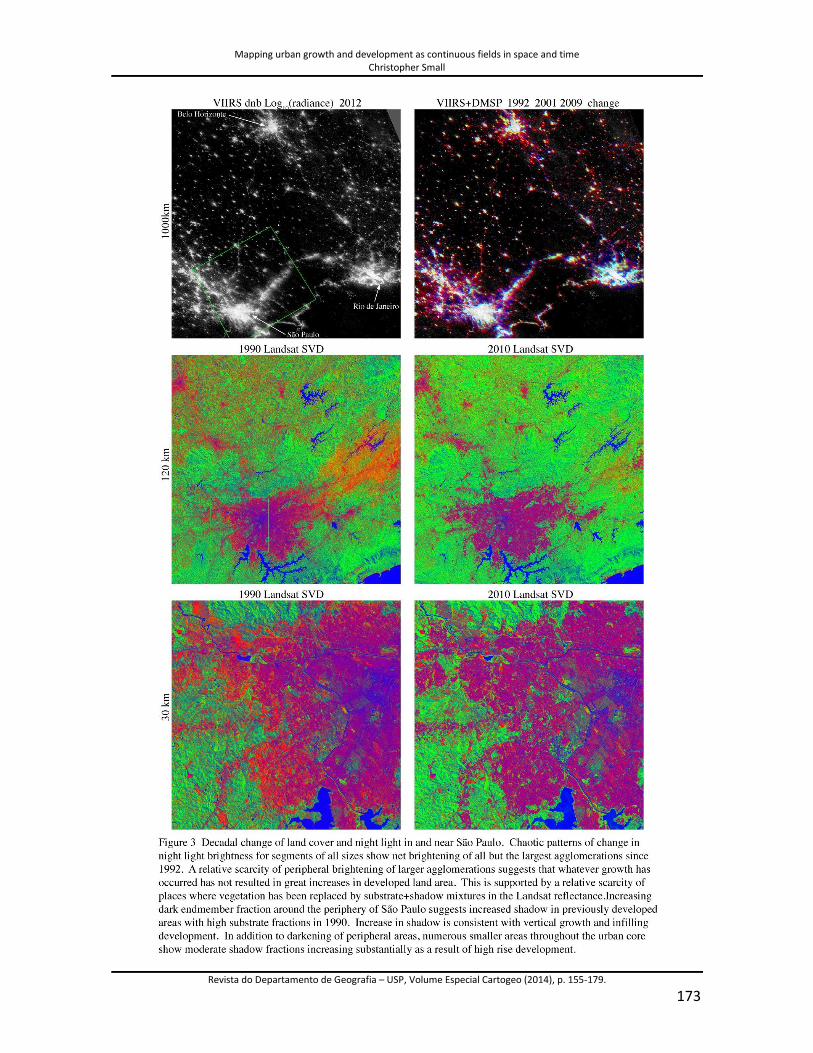
The process of spectral darkening observed in built and lighted areas around the

periphery of São Paulo is an inherently continuous process resulting from increases in

dark fraction below the scale of the pixel. This can be explained physically as an

increase in the area in shadow as building heights increase and infill development

increases shadow fraction in previously illuminated areas. This process occurs in

more recently built up areas around the periphery of São Paulo but also within the

older parts of the city where high rise development has occurred over the past two

decades.

Darkening from low rise development also occurs on the periphery of New Delhi – but

is not observed in the more rapid growth of Beijing or the more stable land cover



162

around Moscow. This kind of information on the changing composition of urban land

cover would be lost in a discrete classification.

Quantifying the Structure of Continuous Fields

Continuous fields and discrete classifications are not mutually exclusive. In fact,

discrete classifications are often derived from continuous fields. The most common

examples are supervised land cover classifications of multispectral imagery. In the

case of supervised classification, training samples are selected for each class and the

moments of the statistical distributions of the samples are used to derive decision

boundaries upon which the classifications are based. However, this approach assumes

that each class has unique, non-intersecting distributions. This assumption is violated

in the case of different land cover classes with similar or indistinguishable spectral

properties. To make matters worse, even accurate classifications are often non-

repeatable without knowledge of the specific training samples used. Since the general

spectral properties of land cover classes are rarely reported in studies using

supervised classification, and sensitivity to selection of training samples is rarely

discussed, the uniqueness of the classification cannot be determined. Fortunately, the

process of discretizing a continuous field need not suffer from these shortcomings.

Simpler approaches are often possible.

The spatial structure and characteristics of continuous fields can be quantified by the

process of segmentation. Applying a threshold to a continuous field produces discrete

segments of the areas where the value of the field exceeds the threshold. Different

thresholds produce different distributions of segments. A simple example is given by

successive thresholding of night light brightness. Given the presence of overglow and

varying definitions of urban extent, it is not clear what level of brightness best

represents an appropriate measure of development for a specific application. Rather

than choosing a single brightness threshold based on arbitrary or ad hoc criteria, a set

of successive thresholds can be applied to the night light brightness field to determine

the sensitivity of the resulting discrete maps to the threshold chosen. This is

illustrated in Figure 7. The results of the segmentation process can be represented by



163

the size distribution of the areas of the discrete segments that result from each

threshold. The effect of different thresholds is reflected in changes in the resulting

segment size distributions.

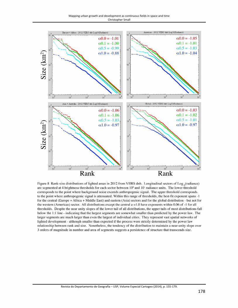
The approach of successive thresholding is applied to the 2012 VIIRS dnb night light

imagery. The imagery is divided into three non-overlapping longitudinal sectors

referred to as western (North and South America), central (Europe, Africa, Middle

East) and eastern (Asia). The dividing longitudes are chosen to avoid breaking any

spatially contiguous lighted areas. For each sector, four different brightness

thresholds are applied to the Log10 of brightness and the size distribution of spatially

continuous lighted areas are calculated. The lower threshold of 1 radiance unit is

selected at the noise floor where background luminance is comparable to the dimmest

anthropogenic lights. The upper threshold of 10 radiance units is chosen at the level

where the smallest anthropogenic lights begin to be completely attenuated. The rank-

size distributions of the segments resulting from these thresholds are shown in Figure

8.

For each threshold the size distribution of segments spans several orders of magnitude

in area. These types of “heavy tailed” Pareto distributions are often represented with

power laws of the form

N = Ax−α

where the number of objects, N, larger than some size, X, follows is determined by the

exponent α and a constant A. The exponent represents the slope of the distribution

when the Log10 of the size of each object is plotted against the Log10 of its ordinal

rank (largest to smallest). The physical meaning of the exponent, or slope of the

distribution, is related to total area of objects of different sizes. Larger negative

exponents correspond to distributions in which large objects account for more total

area than small objects.

Smaller negative exponents correspond to the opposite case where small objects

account for more total area than large objects. A distribution with an exponent of -1

corresponds to the transitional case of a uniform size distribution in which objects of

each size range account for the same total area. In the case of segment areas, the slope



164

of the rank-size distribution, given by the exponent of the best fit power law, indicates

whether larger segments account for more or less total area than smaller segments.

In the case of the size distribution of night lights, different brightness thresholds

produce very similar segment size distributions. For each rank-size distribution of

segment sizes, a power law was fit using the method of (Clauset et al. 2009). The rank-

size distributions and the best fit exponents of the corresponding power laws are

shown in Figure 8. Despite the order of magnitude difference in brightness thresholds,

the shapes of the resulting rank-size distributions are very similar with nearly

identical exponents for the best fit power law of each. The most obvious effect of

increasing the brightness threshold is to reduce both the size and number of segments.

However, the slope is not sensitive to the brightness threshold. This result holds for

each of the three longitudinal sectors and for the global distributions. This implies that

the brightness thresholds produce very similar distributions with nearly equal total

areas of segments of all sizes. However, the largest segments are much larger than

individual cities. They represent vast spatial networks of interconnected

development.

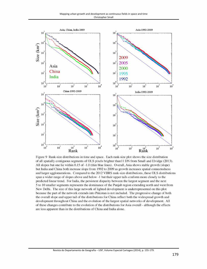
The same approach of discrete segmentation of night light brightness fields can inform

our understanding of how urban systems evolve with time. Figure 9 shows the rank-

size distributions obtained by (Small and Elvidge 2013) for China, India and all of Asia

between 1992 and 2009. Although all of the rank size distributions are well fit by

power laws with exponents very close to -1, the shapes of the upper tails of the

distributions are different for China and India. This reflects real differences in the

spatial structure and size distributions of the urban systems in these two countries.

The process of segmenting night lights at increasing brightness thresholds provides

information on the spatial structure of the brightness field and, by inference, the

spatial structure of the light sources responsible for it. As the threshold is increased

the dimmer peripheral lights connecting the brighter urban cores are attenuated -

causing the larger networks to fragment into smaller subnets. Increasing the

threshold also attenuates the dimmer pixels at the periphery of smaller isolated light

sources causing them to shrink in area. Both fragmentation and shrinkage result in

movement of lighted segments downward through the rank-size distribution. Despite



165

the continuous reordering of the distribution as segments shrink and migrate

downward, the slope of the distribution remains close to -1. The reverse of this

process, decreasing the threshold, is analogous to the urban growth process.

Peripheral growth of small settlements causes them to move up through the

distribution discontinuously at different rates. Spatial coalescence of settlements of all

sizes causes newly joined settlement networks to move upward through the

distribution at varying rates determined by the spatial distribution of light sources of

different sizes. Even though the brightness field is continuous, the process of

successive segmentation can produce discontinuous results with abrupt changes

occurring when two or more segments become connected into a single larger segment.

As a result, the size distribution of segments produced by one threshold can be very

different from the size distribution of segments from a slightly different threshold.

The segment size distribution of lighted areas has a direct relevance to fundamental

questions of urban growth and development. Imposing a threshold on a continuous

field of night light brightness produces a binary map of lighted areas against an

unlighted background. This is analogous to, but different from, city size distributions

based on population residing within administrative units. If areas with night light

brightness above a certain threshold are considered to be urban, segmentation of a

brightness map with a single threshold produces one possible depiction of urban

extent. In the absence of a single such threshold, it is possible to choose multiple

thresholds to see how the resulting distributions change.

Urban Growth and Spatial Networks of Development

City size distributions, defined on the basis of population, are often described as power

laws. Auerbach (Auerbach 1913) made the initial observation that the product of city

population and ordinal rank was approximately constant for Germany. Lotka (Lotka

1941) subsequently reported a hyperbolic rank-size relationship for U.S. city

populations, noting that the slope of the Log10 rank-size plot was not exactly -1 but -

0.93 with some of the larger cities being smaller than predicted. Zipf later estimated



166

that the exponent of the power law is also close to -1 for U.S. cities (Zipf 1942), a

finding that holds for the frequency of usage of words, sizes of firms, and several other

socioeconomic variables (Zipf 1949). He postulated a universal principal of least effort

from which the power law emerges as an optimal distribution for a variety of

processes. The special case of a power law distribution with an exponent of -1 is often

referred to as Zipf's Law; it has been tested repeatedly for cities, yielding mixed but

generally consistent results (Gabaix et al. 2004; Nitsch 2005; Pumain 2004; Soo 2005).

The consistency of Zipf’s Law has attracted sustained interest for several decades, and

been the basis for a multitude of models (Berry and Garrison 1958; Gabaix 1999; Lotka

1941; Pumain 2006) , but the varying degree and extent of agreement with

observation seem to preclude consensus on either the universality of the law (Gan et

al. 2006; Soo 2005) or its underlying causes (Batty 2006a, b; Lotka 1941; Pumain

2004, 2006). On empirical grounds alone, the assertion of a universal power law for

city size remains controversial because the estimates of linearity and slope of the

power law rank-size distribution often vary over time and among countries (Gabaix et

al. 2004; Nitsch 2005; Pumain and Moriconi-Ebrard 1997; Soo 2005). However, these

irregularities may be the result of the way population is measured. Census

enumerations are tied to administrative units. These administrative units may be

appropriate for smaller isolated cities but they impose artificial boundaries on cities

embedded within larger metropolitan areas. The administrative fragmentation of

large agglomerations limits the size of population that can be represented and

precludes the consideration of larger agglomerations in the analysis. Using a more

accurate and consistent spatial depiction of urban areas could avoid some of these

shortcomings and potentially resolve the controversy over Zipf’s Law.

The rank-size distributions of spatially contiguous lighted segments are consistent

with power law distributions with exponents of -1, regardless which brightness

threshold is applied within an order of magnitude of range. This observation

complements previous analyses of city size distribution based on population – but

extends it into the spatial dimension. The fact that the largest contiguous lighted

segments correspond to spatial networks much larger than individual cities suggests

that the regularity of these distributions may be fundamentally related to their spatial



167

structure and the process of urban growth and spatial coalescence of individual

settlements into network structures.

A detailed discussion is beyond the scope of this paper but the result illustrates the

power of the continuous field representation of urban environments and land cover.

Treating night light brightness as a proxy for urban development allows for self-

consistent mapping at global scales – as well as direct comparison to continuous fields

of land cover abundance derived from Landsat observations. Together, these two

continuous field depictions of urban environments allow for retrospective analyses of

urban extent – without relying on ad hoc or arbitrary definitions of what defines

urban.

Depiction of urban areas with continuous fields can be extended to the concept of a

continuum of urban form and function. Taking land cover, and by implication land use,

as a relatively simple example, the continuum of urban form could extend from

completely constructed anthropogenic environments composed only of buildings and

streets to a completely natural environment with no anthropogenic modifications. At

present, discrete land cover maps attempt to represent this structure – but are limited

by the scale dependence and accuracy of the classification procedure. A continuous

field of land cover could provide a viable alternative to the discrete representation for

many applications. Taking population density as a relatively simple example, the

continuum of urban function could extend from very densely populated areas with

large numbers of people engaged in a common activity (e.g. a sports arena filled with

spectators) to very sparsely populated areas where little or no human activity occurs.

At present, discrete census enumerations attempt to represent this structure – but are

limited by the spatial resolution of the census administrative units and the fact that

census enumerations measure where people sleep, not where they work. A

continuous field of ambient population density, derived from a disaggregation of

census data with continuous fields of night light brightness and land cover fractions,

could provide a probability density distribution that accounts for the mobility of

population and the uncertainty in its measurement. As illustrated here, a single

continuous field representation can be segmented as necessary to suit the specific

needs of different applications.



168

ACKNOWLEDGEMENTS

This research was funded most recently by the NASA Land Cover and Land Use Change

Program (grant LCLUC09-1-0023) and Interdisciplinary Science Program (grants

NNX12AM89G & NNN13D876T). The idea of continuous fields of urban land cover and

development evolved from years of discussions with Deborah Balk, Ligia Barrozo, Uwe

Deichmann, Chris Elvidge, Valentina Mara, Cristina Milesi, Mark Montgomery, Reinaldo

Peréz-Machado, Francesca Pozzi and Greg Yetman.

REFERENCES

Adams, J.B., & Gillespie, A.R. (2006). Remote Sensing of Landscapes with Spectral

Images. Cambridge, UK: Cambridge University Press Adams, J.B., Smith, M.O., &

Johnson, P.E. (1986). Spectral mixture modeling; A new analysis of rock and soil types

at the Viking Lander 1 site. Journal of Geophysical Research, 91, 8098-8122

Auerbach, F. (1913). Das Gesetz der Bevolkerungskonzentration. Petermanns

Geographische Mitteilungen, 59, 74-76 Batty, M. (2006a). Heirarchy in cities and city

systems. In D. Pumain (Ed.), Hierarchy in natural and social sciences (pp. 143-168).

Dordrecht Germany: Kluwer Batty, M. (2006b). Hierarchy in cities and city systems. In

D. Pumain (Ed.), Hierarchy in Natural and Social Sciences (pp. 143-168): Springer

Berry, B.J.L., & Garrison, W.L. (1958). Alternate explanations of urban rank-size

relationships. Annals of the Association of American Geographers, 1, 83-91

Clauset, A., Shalizi, C.R., & Newman, M.E.J. (2009). Power-law distributions in empirical

data. SIAM Review, 51, 661-703

Croft, T.A. (1973). Night-time Images of the Earth From Space. Scientific American, 239,

68-79



169

Elvidge, C.D., Baugh, K.E., Kihn, E.A., Kroehl, H.W., & Davis, E.R. (1997). Mapping city

lights with nighttime data from the DMSP operational linescan system.

Photogrammetric Engineering and Remote Sensing, 63, 727-734

Elvidge, C.D., Imhoff, M.L., Baugh, K.E., Hobson, V.R., Nelson, I., Safran, J., Dietz, J.B., &

Tuttle, B.T. (2001). Night-time lights of the world: 1994-1995. Isprs Journal of

Photogrammetry and Remote Sensing, 56, 81-99

Gabaix, X. (1999). Zipf’s law for cities: an explanation. Quarterly Journal of Economics

114, 739–767

Gabaix, X., Ioannides, Y.M., Henderson, J.V., & Jacques-FranÁois, T. (2004). Chapter 53

The evolution of city size distributions. Handbook of Regional and Urban Economics

(pp. 2341-2378): Elsevier Gan, L., Li, D., & Song, S. (2006). Is the Zipf law spurious in

explaining city-size distributions? Economics Letters, 92, 256-262

Lotka, A. (1941). The law of urban concentration. Science, 94, 164

Nitsch, V. (2005). Zipf zipped. Journal of Urban Economics, 57, 86-100

Pumain, D. (2004). Scaling laws and urban systems. In (p. 26). Santa Fe NM: Santa Fe

Institute Pumain, D. (2006). Alternative explanations of heirarchical differentiation in

urban systems. In D. Pumain (Ed.), Hierarchy in natural and social sciences (pp. 169-

222). Dordrecht Germany: Kluwer Pumain, D., & Moriconi-Ebrard, F. (1997). City Size

distributions and metropolisation. Geojournal, 43, 307-314

Small, C., & Elvidge, C.D. (2013). Night on Earth: Mapping decadal changes of

anthropogenic night light in Asia. International Journal of Applied Earth Observation

and Geoinformation, 22, 40-52

Small, C., & Milesi, C. (2013). Multi-scale Standardized Spectral Mixture Models. Remote

Sensing of Environment, 136, 442-454



170

Small, C., Pozzi, F., & Elvidge, C.D. (2005). Spatial Analysis of Global Urban Extent from

DMSP-OLS Night Lights. Remote Sensing of Environment, 96, 277-291

Soo, K.T. (2005). Zipf's Law for cities: a cross-country investigation. Regional Science

and Urban Economics, 35, 239-263

Yu, L., Liang, L., Wang, J., Zhao, Y., Cheng, Q., Hu, L., Liu, S., Yu, L., Wang, X., Zhu, P., Li, X.,

Xu, Y., Li, C., Fu, W., Li, X., Li, W., Liu, C., Cong, N., Zhang, H., Sun, F., Bi, X., Xin, Q., Li, D.,

Yan, D., Zhu, Z., Goodchild, M.F., & Gong, P. (2014). Meta- discoveries from a synthesis

of satellite-based land-cover mapping research. International Journal of Remote

Sensing, 4573-4588

Zipf, G.K. (1942). The Unity of Nature, Least-Action, and Natural Social Science.

Sociometry, 5, 48-62

Zipf, G.K. (1949). Human Behavior and the Principle of Least-Effort: Addison Wesley



171



172



173



174



175



176



177



178



179

mapping urban growth and development as …

Documents