t 107 (2007) 484–495www.elsevier.com/locate/rse

Remote Sensing of Environmen

Mapping sediment-laden sea ice in the Arctic using AVHRR remote-sensingdata: Atmospheric correction and determination of reflectances as a

function of ice type and sediment load

Petra Huck a,b,⁎, Bonnie Light c,1, Hajo Eicken b, Michael Haller a,b,2

a Institut für Meteorologie und Klimaforschung, Universität Karlsruhe (TH), 76131 Karlsruhe, Germanyb Geophysical Institute, University of Alaska Fairbanks, Fairbanks, AK 99775-7320, USAc Department of Atmospheric Sciences, University of Washington, Seattle, WA 98195, USA

Received 18 May 2004; received in revised form 8 September 2006; accepted 1 October 2006

Abstract

Exploiting the fact that the spectral characteristics of light backscattered from sediment-laden ice differ substantially from those of clean iceand that sediment tends to accumulate at the ice surface during the first melt season, remote-sensing techniques provide a valuable tool formapping the extent of particle-laden ice in the Arctic basin and assessing its particulate loading. This study considers two fundamental problemsthat still need to be addressed in order to make full use of satellite observations for this type of assessment: (i) the effects of the atmosphere onsurface reflectances derived from radiances measured by the satellite sensor need to be quantified and ultimately corrected for, and (ii) the spectralreflectance of the ice surface as a function of particle loading and sub-pixel distribution needs to be determined in order to derive quantitativeestimates from the at-sensor satellite signal. Here, spectral albedos have been computed for different ice surfaces of variable sediment load with aradiative transfer model for sea ice coupled with an optical model for particulates included in sea ice. In a second step, the role of the atmospherein modulating the surface reflectance signal is assessed with the aid of an atmospheric radiative transfer model applied to a “standard” Arcticatmosphere and surface boundary conditions as prescribed by the sea ice radiative transfer model. A series of sensitivity studies helps assessdifferences between top-of-the-atmosphere and true surface reflectance and has been utilized to derive a look-up table for atmospheric correctionof Advanced Very High Resolution Radiometer (AVHRR) data over sediment-laden sea ice surfaces. In particular, the effects of solar elevation,viewing geometry, and atmospheric properties are considered. The atmospheric corrections are necessary for certain geometries and surface types.Large discrepancies between raw and corrected data are particularly evident in the derived coverage of clean ice and ice with small sedimentloading.© 2006 Elsevier Inc. All rights reserved.

Keywords: Sea ice; Atmospheric correction; Remote sensing

1. Introduction

Relative to its areal coverage, the Arctic Ocean's sea icecover is of disproportionate importance to the Earth's climateand radiation budget (Curry et al., 1995; Untersteiner et al.,

⁎ Corresponding author. Now at Department of Physics and Astronomy,University of Canterbury, Christchurch, New Zealand.

E-mail address: peh26@student.canterbury.ac.nz (P. Huck).1 Now at Applied Physics Laboratory, Polar Science Center, University of

Washington, Seattle, WA 98105, USA.2 Now at Meteorologisches Institut Hamburg, Universität Hamburg, 20146

Hamburg, Germany.

0034-4257/$ - see front matter © 2006 Elsevier Inc. All rights reserved.doi:10.1016/j.rse.2006.10.002

1990). This critical role is in large part dependent on the large-scale albedo of the summer ice pack (Perovich et al., 2002).Despite its importance, the data base of observations on thealbedo evolution of the ice cover during melt season is not aslarge as required for purposes of effective validation andconstraint of model simulations (Curry et al., 2001; Perovich,1998; Robinson et al., 1992). This is particularly acute for large-scale estimates based on remotely-sensed data. While some ofthe key processes governing albedo evolution of summer seaice, such as melting of the snow cover, establishment of asurface scattering layer in bare ice and the growth and shrinkageof low-albedo melt ponds are reasonably well understood

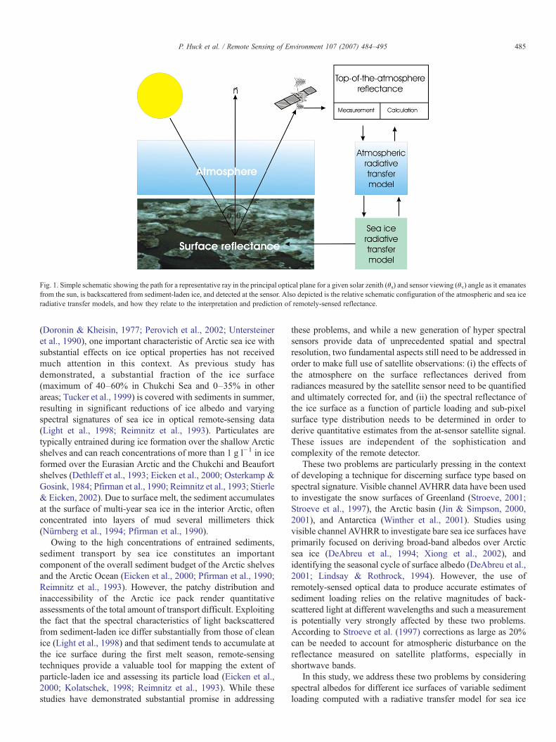
Fig. 1. Simple schematic showing the path for a representative ray in the principal optical plane for a given solar zenith (θs) and sensor viewing (θv) angle as it emanatesfrom the sun, is backscattered from sediment-laden ice, and detected at the sensor. Also depicted is the relative schematic configuration of the atmospheric and sea iceradiative transfer models, and how they relate to the interpretation and prediction of remotely-sensed reflectance.

485P. Huck et al. / Remote Sensing of Environment 107 (2007) 484–495

(Doronin & Kheisin, 1977; Perovich et al., 2002; Untersteineret al., 1990), one important characteristic of Arctic sea ice withsubstantial effects on ice optical properties has not receivedmuch attention in this context. As previous study hasdemonstrated, a substantial fraction of the ice surface(maximum of 40–60% in Chukchi Sea and 0–35% in otherareas; Tucker et al., 1999) is covered with sediments in summer,resulting in significant reductions of ice albedo and varyingspectral signatures of sea ice in optical remote-sensing data(Light et al., 1998; Reimnitz et al., 1993). Particulates aretypically entrained during ice formation over the shallow Arcticshelves and can reach concentrations of more than 1 g l−1 in iceformed over the Eurasian Arctic and the Chukchi and Beaufortshelves (Dethleff et al., 1993; Eicken et al., 2000; Osterkamp &Gosink, 1984; Pfirman et al., 1990; Reimnitz et al., 1993; Stierle& Eicken, 2002). Due to surface melt, the sediment accumulatesat the surface of multi-year sea ice in the interior Arctic, oftenconcentrated into layers of mud several millimeters thick(Nürnberg et al., 1994; Pfirman et al., 1990).

Owing to the high concentrations of entrained sediments,sediment transport by sea ice constitutes an importantcomponent of the overall sediment budget of the Arctic shelvesand the Arctic Ocean (Eicken et al., 2000; Pfirman et al., 1990;Reimnitz et al., 1993). However, the patchy distribution andinaccessibility of the Arctic ice pack render quantitativeassessments of the total amount of transport difficult. Exploitingthe fact that the spectral characteristics of light backscatteredfrom sediment-laden ice differ substantially from those of cleanice (Light et al., 1998) and that sediment tends to accumulate atthe ice surface during the first melt season, remote-sensingtechniques provide a valuable tool for mapping the extent ofparticle-laden ice and assessing its particle load (Eicken et al.,2000; Kolatschek, 1998; Reimnitz et al., 1993). While thesestudies have demonstrated substantial promise in addressing

these problems, and while a new generation of hyper spectralsensors provide data of unprecedented spatial and spectralresolution, two fundamental aspects still need to be addressed inorder to make full use of satellite observations: (i) the effects ofthe atmosphere on the surface reflectances derived fromradiances measured by the satellite sensor need to be quantifiedand ultimately corrected for, and (ii) the spectral reflectance ofthe ice surface as a function of particle loading and sub-pixelsurface type distribution needs to be determined in order toderive quantitative estimates from the at-sensor satellite signal.These issues are independent of the sophistication andcomplexity of the remote detector.

These two problems are particularly pressing in the contextof developing a technique for discerning surface type based onspectral signature. Visible channel AVHRR data have been usedto investigate the snow surfaces of Greenland (Stroeve, 2001;Stroeve et al., 1997), the Arctic basin (Jin & Simpson, 2000,2001), and Antarctica (Winther et al., 2001). Studies usingvisible channel AVHRR to investigate bare sea ice surfaces haveprimarily focused on deriving broad-band albedos over Arcticsea ice (DeAbreu et al., 1994; Xiong et al., 2002), andidentifying the seasonal cycle of surface albedo (DeAbreu et al.,2001; Lindsay & Rothrock, 1994). However, the use ofremotely-sensed optical data to produce accurate estimates ofsediment loading relies on the relative magnitudes of back-scattered light at different wavelengths and such a measurementis potentially very strongly affected by these two problems.According to Stroeve et al. (1997) corrections as large as 20%can be needed to account for atmospheric disturbance on thereflectance measured on satellite platforms, especially inshortwave bands.

In this study, we address these two problems by consideringspectral albedos for different ice surfaces of variable sedimentloading computed with a radiative transfer model for sea ice

Table 1Vertical structure used in sea ice radiative transfer model for calculating surfacealbedo of clean and contaminated snow free sea ice during the melt season

Layer # Thickness (cm) σ (cm−1) g n

1 1 3.3 0.89 1.02 4 3.9 0.89 1.03 20 7.3 0.90 1.34 260 4.8 0.92 1.3

Scattering coefficients (σ), asymmetry parameters (g), and refractive indices (n)are for wavelength 500 nm.

486 P. Huck et al. / Remote Sensing of Environment 107 (2007) 484–495

(Grenfell, 1983, 1991) coupled with an optical model forparticulates included in sea ice (Light et al., 1998). The role ofthe atmosphere in modulating the surface reflectance signal isassessed with the aid of an atmospheric radiative transfer model(6S, Vermote et al., 1997). In particular, effects of solarelevation, viewing geometry, and atmospheric conditions weretaken into account. Fig. 1 shows a simple schematic represent-ing the idealized propagation of sunlight backscattered from theice surface to a satellite receiver and how the two radiativetransfer models were used to carry out this work.

A series of sensitivity studies was used to assess differencesbetween top-of-the-atmosphere (TOA) and true surface reflec-tance and then derive a look-up table for atmospheric correctionof Advanced Very High Resolution Radiometer (AVHRR) dataover sediment-laden sea ice surfaces. While the scope of thiswork was necessarily limited to the consideration of a selectnumber of key cases, these nevertheless help identify thosevariables that most significantly affect the derived reflectancesand point the way towards further, more detailed research.

2. Background

Light et al. (1998) developed a model for the verticaldistribution of particulate loading based on physical data andspectral albedo observations taken in sediment-laden sea ice inthe Eurasian Arctic. This model specifies the sedimentconcentration as a function of depth and the inherent opticalproperties of these particulates. Sediment particulates areassumed to be spherical and to have power law sizedistributions that, for optical purposes, are well represented byan effective radius of 9 μm (Light et al., 1998). This informationis used to calculate vertical profiles of spectral absorption andscattering coefficients. Kolatschek (1998) found that bycomparing the albedo of a variety of ice types at short andlong wavelengths, the ice type can be classified based onsurface type and sediment load. These results were used as thebasis for this work.

Although the strongly wavelength-dependent volume ab-sorption is the same for bulk ice and ice grains constitutingsnow, volume scattering by bare sea ice is generally smaller thanthe volume scattering generated by a snow pack. This results insubstantial differences between the reflectance patterns, or bi-directional reflectance distribution functions (BRDF), for baresea ice and snow surfaces. Because anisotropic reflectance is anintrinsic property of snow and sea ice, their albedos cannot beobtained simply by assuming the albedo is proportional to thereflectance value at a single angular position. Rather, theanisotropic reflectance factor (ARF) specifies the angulardependence of this proportionality.

Perovich (1994) made direct measurements of the ARF forsnow covered, bare, and ponded sea ice. His observations weremade at zenith angles of 0°, 30°, and 60°, azimuth angles from−180° to +180° at 30° intervals, and solar zenith anglesbetween 50° and 60°, and they indicate ARF values for bare icefor AVHRR channels 1 (0.540 to 0.820 μm) and 2 (0.600 to1.120 μm) in the nadir viewing direction of approximately 0.82and 0.73, respectively. Jin and Simpson (1999) used radiative

transfer calculations to predict ARFs of approximately unity forbare sea ice at nadir viewing angles, and they predictconsiderable departure from unity as the viewing angleincreases. However, these calculations contain considerableuncertainty, as the small-scale surface roughness parameters forbare sea ice are highly uncertain, yet are key to this modelcalculation. Resolving these uncertainties and minimizingerrors in assessing the impact of the atmosphere on satellite-measured radiances requires sophisticated studies of thelinkages between BRDFs and surface roughness for differentice types. To our knowledge this data is currently not inexistence. However, given that sea ice in summer has beenshown to be rough on all relevant length scales, we haveconfined our sensitivity studies to nadir viewing geometries andassumed reflectance to be proportional to albedo. This may limitextrapolation of our results to higher sensor viewing angles, butis not easily resolved in the absence of required data orconclusive model studies. This approach was also used forsummer ice by Xiong et al. (2002) where isotropic reflectanceand strictly nadir viewing was assumed for the analysis ofreflectance data from bare and ponded ice. As outlined in moredetail in Section 4 of this study, this limitation has significantimpacts on derived reflectances, however, it is not asconsequential for the classification approach adopted here(with estimates of maximum errors evaluated below).

3. Approach and methods

Our overall approach was to first model the spectral albedofor a variety of surface conditions. These modeled albedos werethen used to help classify the sediment loading associated withAVHRR radiance data. An atmospheric radiative transfer modelwas then used to test the sensitivity of these data to uncertaintiesin sensor viewing geometry, solar angle, and atmosphericconditions.

3.1. Modeling surface albedo

We used a four-stream multilayer radiative transfer model(Grenfell, 1991) to calculate surface spectral albedo for cleanand sediment-laden bare and ponded ice. An optical model forthe vertical profiles of ice structure and inherent opticalproperties was derived from spectral albedo observations inthe Eurasian Arctic (Light et al., 1998). Table 1 summarizes theproperties for bare ice. This profile of optical properties applies

Fig. 2. Modeled surface spectral albedos for bare and ponded ice types underdirect incident illumination with solar zenith angle 50°. Total sediment loading isindicated for each curve.

487P. Huck et al. / Remote Sensing of Environment 107 (2007) 484–495

to the ice for both clean and contaminated cases, as the additionof suspended particulate material (SPM) is expected to have theeffect of increasing the absorption while leaving the scatteringunchanged. For each bare ice case, a four-layer model was usedwith a 1 m thick uppermost layer. Layer thicknesses, scatteringcoefficients (σ) and asymmetry factors (g) are indicated for theice constituting each layer. These profiles were derived fromdata taken when the melt had progressed sufficiently that theuppermost five centimeter layer of the ice where the SPM wereentrained were thoroughly deteriorated and quite porous,scattering less light than the higher scattering 20 cm thicklayer beneath. Note that the air/ice refractive index boundary ismodeled to occur below the uppermost 5 cm.

Ponded ice was also represented in this study. Observationsfrom the Surface Heat Balance of the Arctic Experiment(SHEBA) indicate that the reflectivity of summer melt pondsvaries widely. The range of albedos for clean ponds is dueprimarily to variations in the scattering in the ice underneath thestanding water, not necessarily the pond depth. During thecourse of the SHEBA summer, broad-band pond albedosdropped from the bare ice albedo value to values as low as 0.1.In particular, from 400 nm to 600 nm light pond albedos wereobserved to be 0.2 to 0.25 larger than dark pond values(Perovich et al., 2002). We chose to model observations made atSHEBA of a light pond and a dark pond. Both ponds werespecified to be 0.25 m deep, and to overlie ice with verticallyuniform optical properties. The light pond was modeled withunderlying ice 1 m thick with σ=0.4 cm−1 and g=0.92. Thedark pond was modeled with underlying ice 0.50 m thick withσ=0.32 cm−1 and g=0.92. These scattering coefficients andasymmetry parameters were chosen for use in the modelsimulations to produce agreement with specific cases ofobserved spectral albedo, and result in considerably lessbackscattering than for bare ice.

For bare, snow free ice, a clean case and a series of cases withparticulate concentrations of 25, 50, 75, 100, 200, 300, 400, 500and 1000 g m−3 were specified. Spectral absorption coefficientsfor the particulate material were taken from Light et al. (1998).For simplicity, particulates were specified to remain evenlydistributed in the uppermost 25 cm of the bare ice. For pondedice, total particulate loadings were concentrated within theuppermost 1 cm of the ice beneath the pond water. Thisidealized distribution of particulates is clearly an oversimplifi-cation, but it permits this study to be carried out such that resultsare independent of variations in the vertical distribution of SPM.Furthermore, field observations indicate that SPM are spreadover a wider vertical range as a result of increases in the porosityof the uppermost decimeters of the ice during solar heating andmelting. All albedos were calculated using direct illumination atzenith angle 50°. The results do not vary significantly fromalbedos calculated for diffuse incident irradiance (as used byLight et al., 1998), but we selected the more appropriate clearsky case for this visible channel remote-sensing application.

The model calculated spectral albedos for bare and pondedice types are shown in Fig. 2. At wavelengths above 1000 nm,the curves fall on top one another due to a lack of data on theinherent optical properties of SPM at these wavelengths. Values

of σ, g, and n given in Table 1 were used for the bare ice cases.The albedo for the clean ice case has maximum value at 475 nm,and shows substantial backscattering at wavelengths longerthan 600 nm. Clean pond albedos also show peak values at475 nm, but show considerably less backscatter at λN600 nm.Pond albedos for λN950 nm are reduced to Fresnel reflection atthe surface as strong absorption within the pond eliminates thepossibility of light backscattering from the ice beneath thewater. The contrast between albedos for ice and ponds atλN600 nm results from the strong wavelength dependence ofthe absorption of both pure ice and liquid water, and the lack ofscattering within the pond itself. This feature makes it possibleto discriminate between ice and standing surface water in theretrieval algorithm.

3.2. Remotely-sensed data

Apparent reflectances were derived from AVHRR local areacoverage (LAC) data with a 1.1 km ground-projected instanta-neous field-of-view for each detector element. For the detectionof sediment-laden sea ice, channels 1 (0.540 to 0.820 μm) and 2(0.600 to 1.120 μm) contain information relevant to thediscrimination of sediment-laden ice and were considered inthis study. After applying calibration data, radiances werederived from Level 1b data sets and converted to reflectancesbased on top-of-atmosphere radiative fluxes in the corre-sponding spectral bands. Potential calibration problems, in par-ticular with respect to AVHRR channel 2, which may vary withtime, are difficult to account for in an approach such as this.However, results presented below indicate that the classificationhinges mostly on the channel 1 signal and is much less affectedby errors in channel 2, except for very high pond fractions, whichare only of limited importance in most cases analyzed.

Fig. 3. Ratio of reflectances in channel 1 to channel 2 (ρCh1/ρCh2) as a function ofreflectance in channel 1 (ρCh1) for different snow, ice and water surfaces ascalculated from the 6S radiative transfer model for the “base case”. Simulationswere completed for a wide range of SPM loadings as well as dark and light meltponds, specified in the legend.

488 P. Huck et al. / Remote Sensing of Environment 107 (2007) 484–495

3.3. Atmospheric radiative transfer modeling

The 6S (Second Simulation of the Satellite Signal in theSolar Spectrum) radiative transfer model as coded by Vermoteet al. (1997) was employed in this study to simulate the impactof the atmosphere on the sun–target–sensor path as relevant forremote sensing in the visible and near-infrared part of theelectromagnetic spectrum (see Fig. 1). The model accounts forabsorption as well as multiple Rayleigh scattering by relevantatmospheric constituent gases. Principal absorbing gasesinclude O2, O3, H2O, CO2, CH4, and N2O. Except for O3 andH2O, the rest of the gases are assumed to be uniformly mixed inthe atmosphere. The boundary condition at the lower interface isspecified by the BRDF for a given surface. The version of themodel employed here has been kindly provided by J. Stroeve(National Snow and Ice Data Center, Boulder, Colorado) andintegrates BRDFs relevant for different polar snow and icesurfaces (Stroeve et al., 1997). In this study, we only considerLambertian surfaces, such that the reflectance is proportional tothe albedo. This assumption is necessitated by the unknownBRDF of ice surfaces with entrained SPM. Other relevantboundary conditions, such as atmospheric water vapor profiles,are discussed in more detail in the following section. For eachradiative transfer calculation, the solar zenith (θs) and sensorviewing (θv) angles were specified.

4. Results

4.1. Detection of sediment-laden ice

A set of specified surface and atmospheric conditions alongwith viewing geometry and solar elevation was established as a“base case” and was used for detailed study. This base case wasnot strongly affected by uncertainties in the surface BRDF andhad atmospheric conditions similar to those for the bulk ofuseful remotely-sensed data. The base case had a nadir viewingsensor, a solar zenith angle of 50° (corresponding to 73.5°latitude at summer solstice), Arctic summertime atmosphericconditions with water vapor and temperature profiles from theSHEBA data set (www.joss.ucar.edu/cgi-bin/codiac/projs?SHEBA), maritime aerosol concentrations as specified byVermote et al. (1997), and visibility 50 km (Meyer et al., 1991).Reflectances in the spectral bands corresponding to AVHRRchannels 1 (ρCh1) and 2 (ρCh2) of the NOAA-11 satellite wereanalyzed.

Seventeen different ice, snow, and water surfaces wereconsidered as part of this study. Fig. 3 shows the ratio ofreflectances in channel 1 relative to channel 2 (ρCh1/ρCh2) as afunction of ρCh1 for these 17 cases. These cases include clear,ice-free open water, new snow, melting snow, and ten cases ofsnow free sea ice with particulate loads ranging from 0 to1000 g m− 3. The largest loadings that were tested arerepresentative of maximum SPM concentrations found infirst-year ice (Stierle & Eicken, 2002) and typical for surfaceaccumulations in multi-year ice (Nürnberg et al., 1994). Fourdifferent types of ponded ice were also considered and areindicated in Fig. 3, including melt ponds underlain by sediment-

laden ice with SPM concentrations of 100 and 1000 g m−3. Thespectral albedos for these different surface types were takenfrom Fig. 2.

As is evident from the spread of points in Fig. 3, there is aclear dependence of ρCh1 on the SPM concentration in theuppermost portions of the ice. Due to decreased backscatteringby liquid water relative to sea ice, significant absorption oflonger wavelength light, (i.e., ρCh2), by both pure water andpure ice cause the presence of open water, either completely ice-free or occurring in deeper melt ponds at the surface of sea ice,to shift ρCh1/ρCh2 to values considerably larger than thosecharacteristic of bare ice. In part, the strong sensitivity of ρCh1/ρCh2 may be due to what appears to be an overestimation of thisratio by the 6S code. Based on our sensitivity studies (see moredetailed discussion below), this is believed to be the result of acombination of factors, including unrealistically high openwater albedos (which include wind-roughened open oceancases) assumed by the 6S model, along with overestimation ofthe impacts of water vapor and other atmospheric parameters.The surface albedo simulations summarized in Fig. 2 indicatethat a value of ρCh1/ρCh2 below 2 is more realistic and this isborne out by our more detailed analysis in Section 4.2 below.Nevertheless, due to the potential presence of melt water at theice surface in the form of ponds, varying amounts of sedimentloading can be best discriminated by comparing ρCh1 with theratio ρCh1/ρCh2. Here, we extend the approach of Kolatschek(1998) to include a quantitative assessment of the impact ofsediment load on ice surface reflectance in spectral intervalsrelevant for remote-sensing applications as well as a moredetailed assessment of the impact of the atmosphere onradiances measured at the satellite sensor.

While a number of factors and sources of error preclude adetailed assessment of sediment load based on a simpleregressive relationship, following Kolatschek (1998), we definefour different classes of sediment-laden ice: (i) clean or slightlysediment-laden ice, (ii) light, (iii) medium, and (iv) heavysediment loads. These four classes and two different classes for

Fig. 5. Dependence of surface reflectance for AVHRR channel 1 (ρCh1) and thereflectance ratio of channel 1 to channel 2 (ρCh1/ρCh2) on variations in solarzenith angle θs as determined from atmospheric radiative transfer modelsimulations. θs was varied in 5° intervals with “L” and “H” annotations in thefigure indicating the sequence of simulations from lowest (at 35°) to highest (at75°) solar zenith angle for the spread of data points. Sensor viewing angle washeld constant at nadir.

489P. Huck et al. / Remote Sensing of Environment 107 (2007) 484–495

ponded ice and one for open water, with their classificationboundaries, are designated in Fig. 4. Since this study isconcerned with determining sediment loading from AVHRRdata in a conservative fashion, the boundaries between differentclasses aim to minimize the misclassification for sediment-ladenice, while allowing for potentially larger classification errors fornon-sediment-laden ice types and open water. Hence, thepresent classification will likely overestimate the fractions ofopen water and clean, ponded ice, but this is not deemedproblematic within the confined aims of this study.

Errors in AVHRR channel 2 reflectances suggest that thereshould be significant uncertainties on the classification linesdrawn in this figure. In particular, such errors would suggest thathorizontal lines in the classification should have significantuncertainty. This will cause errors in the discrimination betweenbare (both clean and dirty) and ponded (both clean and dirty) ice,but has less effect on the estimation of actual sediment loading.This is particularly true for potential overestimates in ρCh1/ρCh2as we are excluding heavily ponded ice and open water fromfurther analysis (see also Section 4.2 below).

4.2. Sensitivity studies

Based on the geometry of the AVHRR viewing platform, θsfor a single AVHRR scene can vary by as much as 5°and θv by asmuch as 7°. We wish to test the sensitivity of our classificationtechnique to appropriate variations in θs and θv.

For strictly nadir viewing, we varied θs in 5-degree steps from35 to 75° for different surface types in the base case. The resultsof these simulations are shown in Fig. 5 and show a strongdependence of ρCh1 on θs for clean and sediment-laden icecases. This dependence is most pronounced for low sedimentloadings, where ρCh1 varies by as much as 0.1. The reverse holdstrue for open water surfaces and ponded ice, where ρCh1/ρCh2shows strong dependence on θs.

Fig. 6 shows calculations where θs is held constant at 50°and θv varied at 5° intervals between 0° and 70°. Under theseconditions, the sensitivity of ρCh1 and ρCh1/ρCh2 behave

Fig. 4. Classification of four types of sediment loaded ice, two types of pondedice (clean ponds I and sediment-laden ponds II) and open water.

similarly to the sensitivities exhibited in response to changesin θs. Increases in θv produce large changes in ρCh1/ρCh2 foropen water and large changes in ρCh1 for snow and clean anddirty ice.

The sensitivity studies underscore the fact that both thepresence of open water (including in the form of deep meltponds) and new snow can introduce significant classificationerrors. New snow is thought to be less of a problem as it is clearlydistinguished from clean ice and furthermore during the monthsof June and July, in particular under clear sky conditionssnowfall is not expected to be a significant problem. While the

Fig. 6. Dependence of surface reflectance for AVHRR channel 1 ρCh1 and thereflectance ratio of channel 1 to channel 2 ρCh1/ρCh2 on variations in sensorviewing angle θv as determined from radiative transfer model simulations. θvwas varied in 5° intervals with “L” and “H” annotations in the figure indicatingthe sequence of simulations from lowest (at 0°) to highest (at 70°) sensorviewing angle. Solar zenith angle is constant at 50°.

Table 3Correction coefficients a and b for channel 2

490 P. Huck et al. / Remote Sensing of Environment 107 (2007) 484–495

classification scheme effectively eliminates open water andheavily ponded ice from the analysis, this approach requires thatno mixed-pixels containing two different surface types areanalyzed. In the landfast ice case study discussed in Section 4.4below, we know this to be the case with respect to openwater anddeeply ponded ice. However, in cases where it is not possible toexclude contamination by open water, such as in the marginal icezone where floe sizes are generally small, it may be necessary todetermine the fraction of open water and deep ponds using otherremote-sensing observations and then correcting for thepresence of open water through application of a linear mixingmodel that accounts for the areal fraction of open water. In theabsence of such independent data, it may be possible in theory toseparate out the fractions of open water and sediment-laden icebased on their different ρCh1 and ρCh1/ρCh2 signatures. However,uncertainties and errors in determination of the endmember tiepoints may render such an approach impractical.

The sensitivity of derived reflectances to other variables,including variations in the atmospheric temperature and watervapour profile (several profiles over the Arctic summermeasured during the SHEBA experiment have been tested),visibility, and slight differences in band width and center-frequency for different AVHRR sensor types, was assessed.

Table 2Correction coefficients a and b for channel 1

Xiong et al. (2002) found that in particular for AVHRR channel 2uncertainties in the water vapor profile can account for as muchas 15–25% uncertainty in derivation of broadband albedo, withan uncertainty below 5% for channel 1. Here, we observed thatwithin the range of temporal and spatial variations characteristicof the Arctic, none of the aforementioned parameters (whenexamined in conjunction) affected the classification of bare andsediment-laden ice to a significant degree and they have hencenot been considered further.

A rather surprising factor is that Arctic haze does not have anysignificant impact on the sensitivity of the reflectances. In the 6Scode, users specify either the assumed visibility in km or theaerosol optical depth at 550 nm.We chose to specify the visibilityand looked at different values from 10 to 100 km in 10 km steps. Itshowed that the ρCh1 versus ρCh1/ρCh2 relationship was affectedby the change in visibility only for the open water cases. Meyeret al. (1991) state that a visibility of 45 km is often observedduring Arctic spring. It can go down to 12 km during Arctic hazebut that still did not affect the classification of snow and icesurfaces in the sensitivity studies. Furthermore, we note thatArctic haze is mostly confined to the months of Decemberthrough April, with maximum impact in March and early April(Barrie, 1986; Shaw, 1995).With changes in atmospheric stability

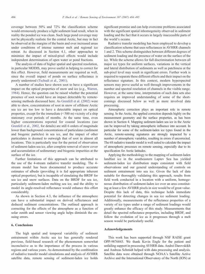
Fig. 7. Example scene (30 June 2000) before and after atmospheric correction, along with corresponding scatter diagrams as applied to sediment-laden ice classification(blue— openwater, yellow/orchid— ponded ice I/II (clean/sediment-laden pond, see Fig. 4), maroon— clean ice/traces of sediments, cyan/green/red— light/medium/high sediment load). (For interpretation of the references to colour in this figure legend, the reader is referred to the web version of this article.)

491P. Huck et al. / Remote Sensing of Environment 107 (2007) 484–495

and warming, Arctic haze abates to background aerosol levelsfrom May onwards (Barrie, 1986; Shaw, 1995).

4.3. Atmospheric correction of AVHRR data

As demonstrated by the model simulations and sensitivitystudies in the preceding sections, estimating the proportion of

sediment-laden ice over polar sea-ice surfaces requires atmo-spheric correction of reflectance data. Given the general lack ofrelevant atmospheric data for specific locations and overflights,and considering the moderate sensitivity and limited variationin the critical atmospheric variables for clear-sky, early to mid-summer conditions which are of relevance in the study ofsediment-laden ice, we propose a generalized approach to

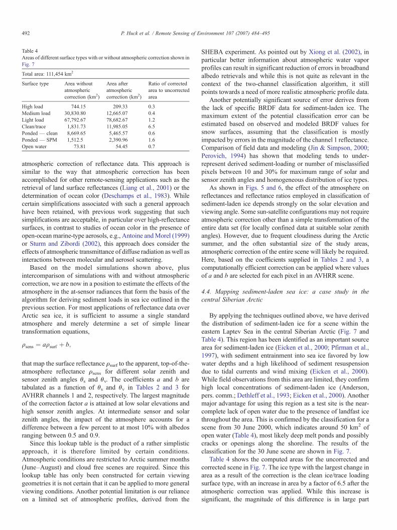
Table 4Areas of different surface types with or without atmospheric correction shown inFig. 7

Total area: 111,454 km2

Surface type Area withoutatmosphericcorrection (km2)

Area afteratmosphericcorrection (km2)

Ratio of correctedarea to uncorrectedarea

High load 744.15 209.33 0.3Medium load 30,830.80 12,665.07 0.4Light load 67,792.67 78,682.67 1.2Clean/trace 1,831.73 11,985.05 6.5Ponded — clean 8,669.65 5,465.57 0.6Ponded — SPM 1,512.5 2,390.96 1.6Open water 73.81 54.45 0.7

492 P. Huck et al. / Remote Sensing of Environment 107 (2007) 484–495

atmospheric correction of reflectance data. This approach issimilar to the way that atmospheric correction has beenaccomplished for other remote-sensing applications such as theretrieval of land surface reflectances (Liang et al., 2001) or thedetermination of ocean color (Deschamps et al., 1983). Whilecertain simplifications associated with such a general approachhave been retained, with previous work suggesting that suchsimplifications are acceptable, in particular over high-reflectancesurfaces, in contrast to studies of ocean color in the presence ofopen-ocean marine-type aerosols, e.g., Antoine andMorel (1999)or Sturm and Zibordi (2002), this approach does consider theeffects of atmospheric transmittance of diffuse radiation as well asinteractions between molecular and aerosol scattering.

Based on the model simulations shown above, plusintercomparison of simulations with and without atmosphericcorrection, we are now in a position to estimate the effects of theatmosphere in the at-sensor radiances that form the basis of thealgorithm for deriving sediment loads in sea ice outlined in theprevious section. For most applications of reflectance data overArctic sea ice, it is sufficient to assume a single standardatmosphere and merely determine a set of simple lineartransformation equations,

qsens ¼ aqsurf þ b;

that map the surface reflectance ρsurf to the apparent, top-of-the-atmosphere reflectance ρsens for different solar zenith andsensor zenith angles θs and θv. The coefficients a and b aretabulated as a function of θs and θv in Tables 2 and 3 forAVHRR channels 1 and 2, respectively. The largest magnitudeof the correction factor a is attained at low solar elevations andhigh sensor zenith angles. At intermediate sensor and solarzenith angles, the impact of the atmosphere accounts for adifference between a few percent to at most 10% with albedosranging between 0.5 and 0.9.

Since this lookup table is the product of a rather simplisticapproach, it is therefore limited by certain conditions.Atmospheric conditions are restricted to Arctic summer months(June–August) and cloud free scenes are required. Since thislookup table has only been constructed for certain viewinggeometries it is not certain that it can be applied to more generalviewing conditions. Another potential limitation is our relianceon a limited set of atmospheric profiles, derived from the

SHEBA experiment. As pointed out by Xiong et al. (2002), inparticular better information about atmospheric water vaporprofiles can result in significant reduction of errors in broadbandalbedo retrievals and while this is not quite as relevant in thecontext of the two-channel classification algorithm, it stillpoints towards a need of more realistic atmospheric profile data.

Another potentially significant source of error derives fromthe lack of specific BRDF data for sediment-laden ice. Themaximum extent of the potential classification error can beestimated based on observed and modeled BRDF values forsnow surfaces, assuming that the classification is mostlyimpacted by errors in the magnitude of the channel 1 reflectance.Comparison of field data and modeling (Jin & Simpson, 2000;Perovich, 1994) has shown that modeling tends to under-represent derived sediment-loading or number of misclassifiedpixels between 10 and 30% for maximum range of solar andsensor zenith angles and homogeneous distribution of ice types.

As shown in Figs. 5 and 6, the effect of the atmosphere onreflectances and reflectance ratios employed in classification ofsediment-laden ice depends strongly on the solar elevation andviewing angle. Some sun-satellite configurations may not requireatmospheric correction other than a simple transformation of theentire data set (for locally confined data at suitable solar zenithangles). However, due to frequent cloudiness during the Arcticsummer, and the often substantial size of the study areas,atmospheric correction of the entire scene will likely be required.Here, based on the coefficients supplied in Tables 2 and 3, acomputationally efficient correction can be applied where valuesof a and b are selected for each pixel in an AVHRR scene.

4.4. Mapping sediment-laden sea ice: a case study in thecentral Siberian Arctic

By applying the techniques outlined above, we have derivedthe distribution of sediment-laden ice for a scene within theeastern Laptev Sea in the central Siberian Arctic (Fig. 7 andTable 4). This region has been identified as an important sourcearea for sediment-laden ice (Eicken et al., 2000; Pfirman et al.,1997), with sediment entrainment into sea ice favored by lowwater depths and a high likelihood of sediment resuspensiondue to tidal currents and wind mixing (Eicken et al., 2000).While field observations from this area are limited, they confirmhigh local concentrations of sediment-laden ice (Anderson,pers. comm.; Dethleff et al., 1993; Eicken et al., 2000). Anothermajor advantage for using this region as a test site is the near-complete lack of open water due to the presence of landfast icethroughout the area. This is confirmed by the classification for ascene from 30 June 2000, which indicates around 50 km2 ofopen water (Table 4), most likely deep melt ponds and possiblycracks or openings along the shoreline. The results of theclassification for the 30 June scene are shown in Fig. 7.

Table 4 shows the computed areas for the uncorrected andcorrected scene in Fig. 7. The ice type with the largest change inarea as a result of the correction is the clean ice/trace loadingsurface type, with an increase in area by a factor of 6.5 after theatmospheric correction was applied. While this increase issignificant, the magnitude of this difference is in large part

493P. Huck et al. / Remote Sensing of Environment 107 (2007) 484–495

explained by the fact that in the raw scene very little unpondedclean ice has been identified. With the location of the classboundary chosen so as to minimize classification errors forsediment-laden ice, even a small shift of channel 2 radiancesresults in a significant relative increase in clean ice area.However, overall these numbers are still small compared toponded or sediment-laden ice. The estimated area of heavilysediment loaded ice changed the least as a result of thecorrection. In discussing the areas of different ice types, it needsto be kept in mind that potential calibration errors of AVHRRchannel 2 may add to the classification error. However, asoutlined in more detail above, the sensitivity studies clearlydemonstrate that classification results are much more sensitiveto changes in channel 1 radiances, which are associated with amuch smaller calibration error.

In mapping sediment-laden ice, scenes should be obtainedfor which the snow cover has completely melted away withsome melt of surface ice layers resulting in concentration ofsediments in the surface layers. This is typically the case fromearly to mid-June onwards well into the month of July. Laterseason images are less desirable because of substantial thinningof the ice and the corresponding decrease in albedo. With such acomparatively narrow window in time and persistent cloudcover, typically only a few suitable scenes can be obtained forany given year in the study area, with substantial portions of theregion having to be masked out for cloud cover (as in Fig. 7).The distribution of sediments shown in Fig. 7 is in line with thelimited field observations available for this region, showingsediment-laden ice prevalent in the coastal, near-shore areas (inparticular off the major river deltas, such as the Lena Delta) andthe northeastern regions of the study area, where strong tidalcurrents and low water depths exist towards the New SiberianIslands (Eicken et al., 2000).

Overall the impact of the atmospheric correction scheme is toreduce the area of high and medium sediment-load ice whileincreasing that of light sediment-load and clean ice (Table 4).This is evident from the scatter plots of band ratios for ρCh1/ρCh2 plotted vs. ρCh1 where there is a general shift in the icereflectances towards higher values of ρCh1.

One of the few data sets available for validation of theapproach is that of Dethleff et al. (1993), who sampled sea ice ata few selected locations in the southeastern Laptev Sea in springof 1992. They reported overall low sediment loading (mostlybetween b10 and 100 mg l−1) in the landfast ice which agreeswell with satellite-derived maps for that year indicating nohighly sediment-laden ice, b0.3% medium sediment load, 65%light sediment load, and 33% clean ice.

5. Discussion

We have described an approach (following Kolatschek,1998) to map the distribution of sediment-laden Arctic sea icebased on the impact of particulate inclusions at variousconcentrations on optical properties of the ice and hencesurface reflectance. Simple assessments of this, both in thisstudy and in Kolatschek (1998) and Eicken et al. (2000),indicate that this method holds considerable promise and

reliably distinguishes between different forms of sediment-laden and clean sea ice. For homogeneous, pure endmember icesurfaces present within a given pixel, modeling and a sensitivitystudy indicate a complete separation between the differentprevailing ice surfaces (Fig. 3). What is not clear at present, ishow variations in the vertical distribution and types ofsediments impact the bulk optical properties of the ice. Basedon earlier modeling studies (Light et al., 1998) and what isknown about the composition and distribution of sediment-laden ice in the Arctic (Nürnberg et al., 1994) it appears that thegreatest source of error is the vertical SPM profile in the ice.Thus, in the later stages of melt, sediments tend to accumulate inoptically opaque surface layers (Nürnberg et al., 1994), whichmay preclude a more detailed distinction between differentsediment loadings. While model simulations (Light et al., 1998)suggest that these changes in vertical distribution result inchanges in surface reflectance, frequent and dense cloud covercause difficulties in monitoring these time-dependent late-summer changes from satellite based sensors. However, a fieldstudy of changes in optical properties of sediment-laden sea iceundergoing melt may be quite useful in estimating the relativeimportance of this process. This would be particularly useful forconsidering spatial and temporal changes in the inherent opticalproperties of SPM. These quantities have been held fixedin this study, as we are not aware of information about theirevolution.

The other major uncertainty with respect to the distribution ofsediments is the horizontal inhomogeneity of sediment con-centration. Typically, sediment-laden ice has a patchy occurrenceat the spatial scales relevant for satellite remote-sensing (Stierle &Eicken, 2002). However, the near-linear dependence of reflectanceon sediment loading up to SPM concentrations of several hundredmg l−1 suggests that sub-pixel scale mixing effects may not be ascritical as vertical variability. Of greater importance is thedistribution of melt ponds on the ice surface. Due to the higherabsorption in the near-IR (AVHRR channel 2), the presence of aliquid water layer has the tendency to shift values towards higherratios of ρCh1/ρCh2 while at the same time lowering the overallmagnitude of ρCh1 (Fig. 3). Here, this impact on the reflectancesignal has been taken into account by only considering data pointswith low ρCh1/ρCh2 values for the mapping of sediment-laden ice.However, as suggested by the area fractions of ponded ice (Table 4)which in many cases are lower by as much as a factor of 2–4 thanthose expected on level landfast ice, the presence of ponds at the sub-pixel scale may still impact measurements to some extent. The errordue to this effect will be small in the early melt season when pondalbedos are comparatively high (0.5–0.6) and area fractions stillmodest (0.1–0.2), but may result in more substantial misclassifica-tions later in the season as ponds deepen, drop in albedo (0.1–0.2),and increase in area fractional coverage (N0.2) (Perovich et al.,2002).

While we did not explicitly calculate the effects of sub-pixelponding and open water on this classification scheme, we usedthe points in Fig. 3 to estimate some of these effects and theirassociated errors. An obvious misclassification of sedimentloading would result from the case where a pixel contains cleanice and melt ponds, but no sediment. For melt pond fractional

494 P. Huck et al. / Remote Sensing of Environment 107 (2007) 484–495

coverage between 50% and 72% the classification schemewould erroneously produce a light sediment load result, when inreality the ponded ice was clean. Such large pond coverage maynot be physically realistic for the central Arctic, but may in factbe observed at the margins of the basin and over increased areasunder conditions of intense summer melt and regional iceretreat. As discussed in Section 4.1, other approaches tominimize the impact of mixed-pixel effects would includeindependent determination of open water or pond fractions.

The analysis of data of higher spatial and spectral resolution,in particular MODIS, may prove useful in helping to correct forthis effect. However, field measurements are required as well,since the overall impact of ponds on surface reflectance ispoorly understood (Tschudi et al., 2001).

A number of studies have shown soot to have a significantimpact on the optical properties of snow and ice (e.g., Warren,1984). Hence, the question can be raised whether the potentialpresence of soot would have an impact detectable by remote-sensing methods discussed here. As Grenfell et al. (2002) wereable to show, concentrations of soot in snow of offshore Arcticsea ice are too low to have a detectable impact on opticalproperties, except for the immediate (b500 m) vicinity of a shipstationary over periods of months. At the same time, evenhigher concentrations reported for coastal locations (seeGrenfell et al., 2002, for details) are still 6 orders of magnitudelower than background concentrations of particulates (sedimentand biogenic particles) in sea ice, and the impact of otherparticulates is deemed to outweigh that of soot in almost alllocations. This is particularly true for the period of observationof sediment-laden sea ice, after complete removal of snow coverand accumulation of sedimentary and biogenic impurities at thesurface of the ice.

Further limitations of this approach can be attributed tothe use of the 4-stream radiative transfer modeling. The 4-stream model has been documented to produce accurateestimates of albedo (providing it is fed appropriate inherentoptical properties), but is incapable of simulating the BRDF forsea ice and snow surfaces. Data on the BRDF for sea ice,particularly sediment-laden melting sea ice, and the ability tomodel its angle-resolved reflectance would enhance this effortconsiderably.

As shown in Section 4.3, the influence of the atmospherecan have a substantial impact on derived reflectances anddeduced sediment concentrations. The outlined approach incorrecting for the effects of the atmosphere as a function ofsolar zenith and sensor viewing angle helps diminish the en-suing errors.

6. Conclusions

The high spatial and temporal variability of sedimententrainment within Arctic sea ice has generally renderedprevious, field-based research of the phenomenon somewhatinconclusive as to the importance of the process in variousregions and various years. As demonstrated by the combinationof radiative transfer model simulations and analysis of AVHRRsatellite data, remote sensing of sediment-laden ice holds

significant promise and can help overcome problems associatedwith the significant spatial inhomogeneity observed in sedimentloading and the fact that it occurs in largely inaccessible parts ofthe world's oceans.

Radiative transfer modeling has been employed to develop aclassification scheme that uses reflectances in AVHRR channels1 and 2. This scheme distinguishes between different degrees ofsediment loading and the presence of water on the surface of theice. While the scheme allows for full discrimination between allmajor ice types for uniform surfaces, variations in the verticaland lateral distribution of sediments as well as patchiness at thesub-pixel level may result in significant errors. Further work isrequired to separate these different effects and their impact on thereflectance signature. In this context, modern hyperspectralsensors may prove useful as well through improvements in thenumber and spectral resolution of channels in the visible range.However, at the same time, interpretation of such data sets alsorequires an improved understanding of some of the short-comings discussed below as well as more involved dataprocessing.

Atmospheric correction plays an important role in remotesensing. In the Arctic, the applied correction depends highly on themeasurement geometry and the surface properties, as has beenshown in Section 4. Mapping sediment-laden sea ice in the Arcticcan be improved by taking atmospheric influence into account. Inparticular for some of the sediment-laden ice types found in theArctic, remote-sensing signatures are strongly impacted by anumber of atmospheric variables, resulting in errors if uncorrected.The 6S radiative transfer model is well suited to calculate the impactof atmospheric processes on remote sensing, especially due to itsspecification for Arctic latitudes.

Applying the methodology to the mapping of sediment-ladenlandfast ice in the southeastern Laptev Sea has yieldedsediment-laden ice distribution maps consistent with fieldobservations and our general understanding of controls onsediment entrainment into sea ice. Given the lack of datasuitable for thoroughly validating this approach, results fromfield work conducted in a location with a uniform, homoge-neous distribution of sediment-laden ice over an area constitut-ing at least a few AVHRR pixels in size would be of great value.Despite this lack of data, this technique holds immediatepotential for detecting changes in sea ice sediment loading.Additionally, measurements of the reflectance properties of avariety of ice types under a range of sediment loadings wouldgreatly enhance the efficacy of this study. Measurements thatdetail the spectral reflectance properties, including BRDF, andfollow the evolution of ice as it progresses through a meltseason would be particularly useful.

Acknowledgements

This work has been supported through NSF RAISE grantOPP-9876843. We thank Kevin Engle for the patient andunfailing support in processing AVHRR data. Andrei Darovskikhand Andreas Schmidt helped with data processing and analysis.Satellite data were obtained through NOAA's Satellite ActiveArchive and the International Observatory of the North (ION) at

495P. Huck et al. / Remote Sensing of Environment 107 (2007) 484–495

the University of Alaska Fairbanks. B. Light gratefully acknowl-edges support from the Office of Naval Research, Arctic Programunder Grants N00014-97-1-0765 and N00014-03-1-0120.

References

Antoine, D., &Morel, A. (1999). Amultiple scattering algorithm for atmosphericcorrection of remotely sensed ocean colour (MERIS instrument): Principleand implementation for atmospheres carrying various aerosols includingabsorbing ones. International Journal of Remote Sensing, 20, 1875−1916.

Barrie, L. (1986). Arctic air-pollution — An overview of current knowledge.Atmospheric Environment, 20, 643−663.

Curry, J. A., Schramm, J. L., & Ebert, E. E. (1995). Sea ice-albedo climatefeedback mechanism. Journal of Climate, 8, 240−247.

Curry, J. A., Schramm, J. L., Perovich, D. K., & Pinto, J. O. (2001). Applicationsof SHEBA/FIRE data to evaluation of snow/ice albedo parameterizations.Journal of Geophysical Research, 106, 15,345−315,355.

DeAbreu, R. A., Key, J., Maslanik, J. A., Serreze, M. C., & LeDrew, E. F.(1994). Comparison of in-situ and AVHRR-derived broad-band albedo overArctic sea ice. Arctic, 47, 288−297.

DeAbreu, R. A., Yackel, J., Marber, D., & Arkett, M. (2001). Operationalsatellite sensing of Arctic first-year sea ice melt. Canadian Journal ofRemote Sensing, 27, 487−501.

Deschamps, P. Y., Herman, M., & Tanré, D. (1983). Modeling of theatmospheric effects and its application to the remote sensing of oceancolor. Applied Optics, 22(23), 3,751−3,758.

Dethleff, D., Nürnberg, D., Reimnitz, E., Saarso, M., & Savchenko, Y. P. (1993).East Siberian Arctic Region Expedition '92: The Laptev Sea — Itssignificance for Arctic sea ice formation and transpolar sediment flux.Berichte zur Polarforschung, 120, 3−37.

Doronin, Y. P., & Kheisin, D. E. (1977). Sea ice. New Delhi: Amerind Publ. Co.Eicken, H., Kolatschek, J., Freitag, J., Lindemann, F., Kassens, H., &

Dmitrenko, I. (2000). Identifying a major source area and constraints onentrainment for basin-scale sediment transport by Arctic sea ice. Geophy-sical Research Letters, 27(13), 1,919−1,922.

Grenfell, T. C. (1983). A theoretical mode of the optical properties of sea ice inthe visible and near infrared. Journal of Geophysical Research, 88,9,723−9,735.

Grenfell, T. C. (1991). A radiative transfer model for sea ice with verticalstructure variations. Journal of Geophysical Research, 96, 16,991−17,001.

Grenfell, T. C., Light, B., & Sturm, M. (2002). Spatial distribution and radiativeeffects of soot in the snow and sea ice during the SHEBA experiment.Journal of Geophysical Research, 107(C10), doi:10.1029/2000JC000414.

Jin, Z. H., & Simpson, J. J. (1999). Bidirectional anisotropic reflectance of snow andsea ice in AVHRR channel 1 and 2 spectral regions— Part I: Theoretical analysis.IEEE Transactions on Geoscience and Remote Sensing, 37, 543−554.

Jin, Z. H., & Simpson, J. J. (2000). Bidirectional anisotropic reflectance of snowand sea ice in AVHRR channel 1 and 2 spectral regions — Part II:Corrections applied to imagery of snow on sea ice. IEEE Transactions onGeoscience and Remote Sensing, 38, 999-1,015.

Jin, Z. H., & Simpson, J. J. (2001). Anisotropic reflectance of snow observedfrom space over the Arctic and its effect on solar energy balance. RemoteSensing of Environment, 75, 63−75.

Kolatschek, J. S. (1998). Sea-ice dynamics and sediment transport in the Arctic:Results from field measurements, remote sensing and modeling (in German).Unpublished PhD, University of Bremen, Bremen.

Liang, S., Fang, H., & Chen, M. (2001). Atmospheric correction of LandsatETM+Land Surface Imagery — Part I: Methods. IEEE Transactions onGeoscience and Remote Sensing, 39(11), 2490−2498.

Light, B., Eicken, H., Maykut, G. A., & Grenfell, T. C. (1998). The effect ofincluded particulates in the optical properties of sea ice. Journal ofGeophysical Research, 103, 27,739−27,752.

Lindsay, R. W., & Rothrock, D. A. (1994). Arctic sea-ice albedo from AVHRR.Journal of Climate, 7, 1,737−1,749.

Meyer, F. G., Curry, J. A., Brock, A., & Radke, L. F. (1991). Springtimevisibility in the Arctic. Journal of Applied Meteorology, 30, 342−357.

Nürnberg,D.,Wollenburg, I., Dethleff, D., Eicken,H.,Kassens, H., Letzig, T., et al.(1994). Sediments in Arctic sea ice— implications for entrainment, transportand release.Marine Geology, 119, 185−214.

Osterkamp, T. E., & Gosink, J. P. (1984). Observations and analyses ofsediment-laden sea ice. Orlando: Academic Press.

Perovich, D. K. (1994). Light reflection from sea ice during the onset of melt.Journal of Geophysical Research, 99, 3,351−3,359.

Perovich, D. K. (1998). Optical properties of sea ice. In M. Leppäranta (Ed.),Physics of ice-covered seas (pp. 195−230). Helsinki: University of Helsinki.

Perovich, D. K., Grenfell, T. C., Light, B., & Hobbs, P. V. (2002). Seasonalevolution of the albedo of multiyear Arctic sea ice. Journal of GeophysicalResearch, 107(C10), 8044.

Pfirman, S., Colony, R., Nürnberg, D., Eicken, H., & Rigor, I. (1997).Reconstructing the origin and trajectory of drifting Arctic sea ice. Journal ofGeophysical Research, 102, 12,575−12,586.

Pfirman, S., Lange, M. A., Wollenburg, I., Schlosser, P., Bleil, U., & Thiede, J.(1990). Sea ice characteristics and the role of sediment inclusions in deep-seadeposition: Arctic–Antarctic comparisons (pp. 187−211). Kluwer AcademicPublishers.

Reimnitz, E.,McCormick,M.,McDougall, K., & Brouwers, E. (1993). Sedimentexport by ice rafting from a coastal Polynya, Arctic Alaska, U.S.A. Arcticand Alpine Research, 25, 83−98.

Robinson, D. A., Serreze, M. C., Barry, R. G., Scharfen, G. R., & Kukla, G.(1992). Large-scale patterns and variability of snowmelt and parameterizedsurface albedo in the Arctic Basin. Journal of Climate, 5, 1,109−1,119.

Shaw, G. E. (1995). The Arctic Haze phenomenon. Bulletin of the AmericanMeteorological Society, 76, 2403−2413.

Stierle, A. P., & Eicken, H. (2002). Sedimentary inclusions in Alaskan coastalsea ice: Small-scale distribution, interannual variability and entrainmentrequirements. Arctic, Antarctic, and Alpine Research, 34, 103−114.

Stroeve, J. (2001). Assessment of Greenland albedo variability from theadvanced very high resolution radiometer Polar Pathfinder data set. Journalof Geophysical Research, 106, 33,989−34,006.

Stroeve, J., Nolin, A., & Steffen, K. (1997). Comparison of AVHRR-derived andin situ surface albedo over the Greenland ice sheet. Remote Sensing ofEnvironment, 62, 262−276.

Sturm, B., & Zibordi, G. (2002). SeaWiFS atmospheric correction by anapproximate model and vicarious calibration. International Journal ofRemote Sensing, 23, 489−501.

Tschudi, M. A., Curry, J. A., & Maslanik, J. A. (2001). Airborne observations ofsummertime surface features and their effect on surface albedo during FIRE/SHEBA. Journal of Geophysical Research, 106, 15,335−15,344.

Tucker III, W. B., Gow, A. J., Meese, D. A., & Bosworth, H. W. (1999). Physicalcharacteristics of summer sea ice across the Arctic Ocean. Journal ofGeophysical Research, 104, 1489−1504.

Untersteiner, N., Grantz, A., Johnson, L., & Sweeney, J. F. (1990). Structure anddynamics of the Arctic Ocean ice cover. Geological Society of America,37−51.

Vermote, E. F., Tanré, D., Deuzé, J. L., Herman, M., & Morcrette, J. J. (1997).Second simulation of the satellite signal in the solar spectrum, 6S: Anoverview. IEEE Transactions on Geoscience and Remote Sensing, 35(3),675−685.

Warren, S. G. (1984). Impurities in snow: Effects on albedo and snowmelt.Annals of Glaciology, 5, 177−179.

Winther, J. G., Jespersen, M. N., & Liston, G. E. (2001). Blue-ice areas inAntarctica derived from NOAA AVHRR satellite data. Journal ofGlaciology, 47, 325−334.

Xiong, X. Z., Stamnes, K., & Lubin, D. (2002). Surface albedo over the ArcticOcean derived from AVHRR and its validation with SHEBA data. Journalof Applied Meteorology, 41, 413−425.