mapping regional inundation with spaceborne l-band sar
TRANSCRIPT

City University of New York (CUNY) City University of New York (CUNY)
CUNY Academic Works CUNY Academic Works
Publications and Research City College of New York
2015
Mapping Regional Inundation with Spaceborne L-Band SAR Mapping Regional Inundation with Spaceborne L-Band SAR
Bruce Chapman California Institute of Technology
Kyle MacDonald CUNY City College
Masanobu Shimada Japan Aerospace and Exploration Agency
Ake Rosenqvist SoloEO
Ronny Schroeder California Institute of Technology
See next page for additional authors
How does access to this work benefit you? Let us know!
More information about this work at: https://academicworks.cuny.edu/cc_pubs/488
Discover additional works at: https://academicworks.cuny.edu
This work is made publicly available by the City University of New York (CUNY). Contact: [email protected]

Authors Authors Bruce Chapman, Kyle MacDonald, Masanobu Shimada, Ake Rosenqvist, Ronny Schroeder, and Laura Hess
This article is available at CUNY Academic Works: https://academicworks.cuny.edu/cc_pubs/488

Remote Sens. 2015, 7, 5440-5470; doi:10.3390/rs70505440
remote sensing ISSN 2072-4292
www.mdpi.com/journal/remotesensing
Article
Mapping Regional Inundation with Spaceborne L-Band SAR
Bruce Chapman 1,*, Kyle McDonald 1,2, Masanobu Shimada 3, Ake Rosenqvist 4,
Ronny Schroeder 1,5 and Laura Hess 6
1 Jet Propulsion Laboratory, California Institute of Technology, Pasadena, CA 91109, USA 2 CUNY Environmental Crossroads Initiative and CREST Institute, The City College of New York,
City University of New York, New York, NY 10031, USA; E-Mail: [email protected] 3 Earth Observation Research Center, Japan Aerospace and Exploration Agency, Tsukuba 305-8505,
Japan; E-Mail: [email protected] 4 SoloEO, Tokyo 305-8505, Japan; E-Mail: [email protected] 5 Institute of Botany, University of Hohenheim, D-70593 Stuttgart, Germany;
E-Mail: [email protected] 6 Earth Research Institute, University of California, Santa Barbara, CA 93106, USA;
E-Mail: [email protected]
* Author to whom correspondence should be addressed; E-Mail: [email protected];
Tel.: +1-818-354-3603; Fax: +1-818-393-3077.
Academic Editors: Alisa L. Gallant and Prasad S. Thenkabail
Received: 6 November 2014 / Accepted: 13 April 2015 / Published: 30 April 2015
Abstract: Shortly after the launch of ALOS PALSAR L-band SAR by the Japan Space
Exploration Agency (JAXA), a program to develop an Earth Science Data Record (ESDR)
for inundated wetlands was funded by NASA. Using established methodologies, extensive
multi-temporal L-band ALOS ScanSAR data acquired bi-monthly by the PALSAR instrument
onboard ALOS were used to classify the inundation state for South America for delivery as
a component of this Inundated Wetlands ESDR (IW-ESDR) and in collaboration with JAXA’s
ALOS Kyoto and Carbon Initiative science programme. We describe these methodologies and
the final classification of the inundation state, then compared this with results derived from
dual-season data acquired by the JERS-1 L-band SAR mission in 1995 and 1996, as well as
with estimates of surface water extent measured globally every 10 days by coarser resolution
sensors. Good correspondence was found when comparing open water extent classified from
multi-temporal ALOS ScanSAR data with surface water fraction identified from coarse
resolution sensors, except in those regions where there may be differences in sensitivity to
OPEN ACCESS

Remote Sens. 2015, 7 5441
widespread and shallow seasonal flooding event, or in areas that could be excluded through
use of a continental-scale inundatable mask. It was found that the ALOS ScanSAR
classification of inundated vegetation was relatively insensitive to inundated herbaceous
vegetation. Inundation dynamics were examined using the multi-temporal ALOS ScanSAR
acquisitions over the Pacaya-Samiria and surrounding areas in the Peruvian Amazon.
Keywords: SAR; wetlands; ALOS; inundation; double-bounce
1. Introduction
The lakes, rivers, and wetlands of the lowland Amazon Basin span at least 800,000 square
kilometers [1,4]. Each year the runoff from heavy seasonal rains causes extensive and prolonged
flooding of vegetated environments. These seasonally, semi-permanently or permanently inundated
areas, in addition to forming biologically diverse habitats, also regulate biogeochemical processes such
as the generation of methane and the outgassing of CO2 [2–5]. The flooding dynamics will also be
impacted by any future changes in rainfall and evapotranspiration; some global circulation models
predict that annual rainfall rates in the Amazon Basin could decrease substantially in the next several
decades (e.g., [6,7]). The ability to accurately monitor changes in inundation extent, including
uncertainties and possible biases, would support the study of possible climatological tipping points in
regions where extensive inundation is prevalent [8].
Earth’s globally distributed wetlands are the largest natural sources of methane. However, extensive
disagreements exist between wetland maps and available remotely sensed inundation data sets, in
particular those that specifically target the extent of vegetated wetlands. Of particular note for global
methane modeling, saturated non-inundated wetlands are also important, given that many wetlands will
continue producing methane at depth even if there is no standing water [5].
The flooding dynamics of the wetland areas be can difficult to study by traditional optical
remote sensing techniques due to frequent cloud cover and the difficulty of detecting sub-canopy
inundation [9,10]. One alternative approach is to use a suite of complementary satellite measurements
to estimate factional extent of inundation at a coarse scale [11]; however, these data sets necessitate the
masking of non-wetland areas and could have difficulty detecting inundated areas under the dense forest
canopies in tropical regions [5]. One recent technique consists of using very coarse resolution gravity
data from the National Aeronautics and Space Administration (NASA) Gravity Recovery and Climate
Experiment (GRACE) mission in combination with satellite altimetry data and other sources of data to
estimate the volume of water filling and draining from large wetlands [12,13]. Perhaps, the best results
for the detection of inundated vegetation and open water at fine resolution scales and on large regional
scales (though not yet global) have been obtained through the use of Synthetic Aperture Radar (SAR)
polarimetric backscatter data (e.g., [2,9,14–18]). An important feature of SAR is that cloud cover is
irrelevant to the detection of inundation, and SAR technology therefore allows for a detailed examination
of the seasonal dynamics of the flooding extent at resolutions better than 100 m.
We will describe the development of regional-scale moderate-resolution inundation products based
on space-borne L-band Synthetic Aperture Radar (SAR) data from the Japan Aerospace Exploration

Remote Sens. 2015, 7 5442
Agency’s (JAXA) ALOS PALSAR instrument. ALOS PALSAR data were provided to this task through
an international science program led by JAXA called the Kyoto and Carbon (K&C) initiative. The
objective of the K&C Initiative is to support data and information needs of international environmental
conventions, carbon cycle science, and conservation of the environment. The initiative established a
global systematic observation strategy for ALOS PALSAR that includes repetitive and consistent
mapping of the world’s major wetland regions [19]. For several years, the K&C Initiative was based on
three coordinated themes relating to global biomes (Forests, Wetlands, Deserts and Semi-Arid Regions),
and a fourth theme dealing with the generation of regional ALOS PALSAR mosaics. One of the
motivations of the mosaicking theme lies in the historical context of the Global Rain Forest Mapping
project (GRFM) [19] in which JERS-1 SAR imagery from selected forest areas around the globe
(Southeast Asia, Amazon Basin, Africa, Boreal North America) were calibrated and mosaicked for
further use by the scientific user community.
Since the GRFM project, there have been several technology enhancements that made mosaic
generation more straightforward: path processing of the image strips, reductions in cost of resources,
improved position accuracy for the ALOS satellite, and the existence of a near global high resolution
Digital Elevation Model (DEM) from the Shuttle Radar Topography Mission (SRTM) for
ortho-rectification and calibration [20].
The results of this work, funded by the NASA Making Earth System Data Records for Use in
Research Environments (MEaSUREs) program office, are to become part of an Earth Science Data
Record (ESDR) documenting inundated wetlands.
2. Methodology
The production of regional scale inundation products required the following processing steps:
accurate orthorectification of the data, radiometric terrain correction, relative and absolute calibration
corrections, image mosaicking, and image classification. Many of the described processing steps are
CPU intensive. To facilitate the processing of these data, in particular the ortho-rectification of the data,
some processing was conducted at the NASA Advanced Supercomputing Division located at the NASA
Ames Research Center (NASA Ames, 2014) [21].
2.1. Description of Satellite Data
ALOS PALSAR, an orbiting L-band SAR launched by the JAXA in 2006, pursued a global
observation strategy through the mission’s end of life in April 2011. By restricting both the mode and
the look angle for many of the observations, a time sequence of regionally consistent imagery was
produced [22]. Here, results will be shown from using ALOS PALSAR while it was operating in
ScanSAR mode. When in ScanSAR mode, ALOS PALSAR had a swath width up to a 350 km, a
resolution of 100 m with three looks, and a noise equivalent σ° better than −23 dB [23].
During orthorectification and radiometric calibration of the ALOS ScanSAR data, the DEM generated
by the SRTM mission was utilized. There are several processing versions available for the SRTM DEM,
but this study used SRTM processing version 2.1 [24]. In South America, the pixel spacing was
3 arcseconds, which corresponds to about 90 m at the equator. Vertical height accuracy of this DEM was
found to be better than 7 m in South America [25].

Remote Sens. 2015, 7 5443
JERS-1 SAR was an L-band SAR launched by Japan Aerospace Exploration Agency (then known as
“NASDA”) in 1992 and discontinued operations in 1998. The HH polarization SAR imaged the Earth
at an incidence angle centered at 35 degrees, and at its full resolution of 18 m the data had three looks.
Its noise equivalent σ° was −18 dB [26].
AMSR-E was a dual-polarized total-power passive microwave radiometer provided by JAXA with
12 channels and six frequencies ranging from 6.9 to 89.0 GHz. It was launched onboard the Aqua
satellite and discontinued operations in October 2011. The instrument was designed to measure
precipitation, oceanic water vapor, cloud water, near-surface wind speed, sea surface temperature, soil
moisture, snow cover, and sea ice parameters [27,28].
2.2. Orthorectification and Radiometric Terrain Calibration
Orthorectification of the data consisted of resampling the geocoded slant range data into a well-known
projection and file format. SAR image radiometry is impacted by topographic slope. This terrain-induced
change in backscatter can mimic the signature of inundated wetlands in areas where there should be no
inundated wetlands (i.e., hilly terrain). It is well known how to correct the radiometry of the image for
this effect, but it requires that the imagery be well registered to the topographic data (e.g., [29]). In
addition, the elevation of the ground impacts the geometric translation of the slant range imagery when
projected onto the topographic model of the Earth.
The JAXA Earth Observation Research Centre (EORC) provided ScanSAR mode slant range image
strips for use by the science team of the ALOS K&C Initiative. These ScanSAR image strips were
typically thousands of kilometers in length, but have reduced resolution compared to that obtained during
standard processing. JAXA refers to these image products as “path” image products [30].
First, topographic data were constructed from the publicly available SRTM DEM. Since the image
strips extend across continental-scale regions, we created SRTM—like “tiles” of topography information
corresponding to Universal Transverse Mercator (UTM) zone definitions, each tile therefore being
approximately 6° × 8° in size. The tiles are reconstructed from the SRTM data to be slightly larger than
the strict UTM zone definition to accommodate edge effects. These tiles remained in the standard SRTM
projection, a rectangular latitude/longitude grid with a pixel spacing of 3 arcseconds. Since the ScanSAR
path image products have a spatial resolution of approximately 100 m, the resolutions of the DEM and
ScanSAR imagery are roughly comparable.
For orthorectification and radiometric terrain correction, a software package from Gamma Remote
Sensing [31] was employed. Each processed path image was projected onto the DEM of each UTM zone
that it passed through. To correct residual geolocation errors, the Gamma Remote Sensing package
includes software for well-known techniques for estimating and correcting offsets between images [32].
This software is designed to assist in co-registering pairs of SAR images prior to interfering them, but
also can be used to correct the image geocoding parameters.
Wetland areas in our study regions are challenging, as they are highly dynamic. The rivers and
wetland areas frequently change in appearance and sometimes slightly in location. However, we found
that cross-correlating the imagery against a SAR image based on the SRTM DEM (i.e., as described
in [33]) can be effectively used to determine geocoding errors.
Remote Sens. 2015, 7 5444
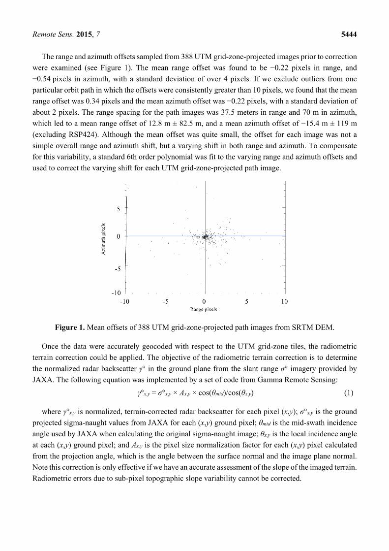
The range and azimuth offsets sampled from 388 UTM grid-zone-projected images prior to correction
were examined (see Figure 1). The mean range offset was found to be −0.22 pixels in range, and
−0.54 pixels in azimuth, with a standard deviation of over 4 pixels. If we exclude outliers from one
particular orbit path in which the offsets were consistently greater than 10 pixels, we found that the mean
range offset was 0.34 pixels and the mean azimuth offset was −0.22 pixels, with a standard deviation of
about 2 pixels. The range spacing for the path images was 37.5 meters in range and 70 m in azimuth,
which led to a mean range offset of 12.8 m ± 82.5 m, and a mean azimuth offset of −15.4 m ± 119 m
(excluding RSP424). Although the mean offset was quite small, the offset for each image was not a
simple overall range and azimuth shift, but a varying shift in both range and azimuth. To compensate
for this variability, a standard 6th order polynomial was fit to the varying range and azimuth offsets and
used to correct the varying shift for each UTM grid-zone-projected path image.
Figure 1. Mean offsets of 388 UTM grid-zone-projected path images from SRTM DEM.
Once the data were accurately geocoded with respect to the UTM grid-zone tiles, the radiometric
terrain correction could be applied. The objective of the radiometric terrain correction is to determine
the normalized radar backscatter γ° in the ground plane from the slant range σ° imagery provided by
JAXA. The following equation was implemented by a set of code from Gamma Remote Sensing:
γ°x,y = σ°x,y × Ax,y × cos(θmid)/cos(θx,y) (1)
where γ°x,y is normalized, terrain-corrected radar backscatter for each pixel (x,y); σ°x,y is the ground
projected sigma-naught values from JAXA for each (x,y) ground pixel; θmid is the mid-swath incidence
angle used by JAXA when calculating the original sigma-naught image; θx,y is the local incidence angle
at each (x,y) ground pixel; and Ax,y is the pixel size normalization factor for each (x,y) pixel calculated
from the projection angle, which is the angle between the surface normal and the image plane normal.
Note this correction is only effective if we have an accurate assessment of the slope of the imaged terrain.
Radiometric errors due to sub-pixel topographic slope variability cannot be corrected.

Remote Sens. 2015, 7 5445
2.3. Relative and Absolute Calibration
Although the data have been generally corrected for radiometric error due to measured slope, errors
in relative and absolute calibration remain in the imagery. Relative calibration errors are generally visible
as brightness trends in the along-track or cross-track directions. Absolute calibration errors are absolute
offsets that are noticeable when examining a temporal sequence of images from the same orbit geometry
and observation mode.
There were several empirical approaches taken to correct for these remaining radiometric errors.
When we use an empirical approach during calibration refinement, we must make some assumptions
that may on occasion be violated. Some environmental conditions will result in changes in
radar-backscattered brightness, and these changes in brightness may be incorrectly interpreted as
calibration errors. When these “calibration errors” are “corrected”, the resultant imagery will actually be
obscuring a real physical change in radar brightness. However, we chose to enforce consistent
radiometry across the multi-temporal sequence of SAR images to more robustly enable the detection of
inundation. Fortunately, the signatures of inundation, open water and inundated vegetation, are generally
quite distinct from second order radiometric changes caused by physical changes in the environment
such as changes in moisture content.
When calibrating the long path image strips from the JAXA EORC path image product, we also must
assume that the relative calibration accuracy may vary in both the along-track and cross-track direction.
We must therefore take care to insure that the average calibration correction applied to any given image
is 0 dB, so as not to introduce absolute calibration errors when calibrating relative calibration errors. The
most common relative calibration error that required correction was visibly apparent as “banding” in the
radiometry, typically aligned in the cross-track direction. Absolute calibration errors were evaluated by
comparing individual images with the average image brightness of the multi-temporal stack of images
Ia, then comparing with the radar image brightness in adjacent UTM grid zones; sometimes several
iterations of calibration were required before the imagery converged to a stable value.
Two simple methods were used to identify and evaluate absolute calibration errors. First,
the ortho-rectified image segments can be stitched into a single image to form a mosaic. There are several
available options for deciding which pixel from multiple images is preserved in the mosaic when a
location on the ground is imaged in more than one pass. The option we chose was to have the far-range
portion of the imagery take precedence over the near range-imagery. We chose this option because the
backscatter from open water can be more variable in the near range due to wind roughening of the water
surface. We ignored zero-fill areas. Second, after a mosaic is constructed, it sometimes is visibly
apparent that adjacent images have a significant difference in brightness. This manifests as a banding
effect within the mosaic and may make it problematic to correctly classify the status of inundation in
wetland areas. We therefore compared individual orthorectified image strips with the average image
brightness of all the images within the UTM grid-zone, then performed the adjustments described below.
The image brightness can vary for a variety of reasons. In addition to environmental factors, the
instrument calibration may be in error, or there may be processing errors introduced at some stage. Given
that the radar backscatter of targets varies with incidence angle and with target type, and given that
ScanSAR data have a wide range of incidence angles within a swath (from 20°+ to 40°+), some banding
may be due to the varying nature of the scattering of whatever is on the ground. Recent changes in

Remote Sens. 2015, 7 5446
moisture content of vegetation and/or ground soils can result in significant changes in backscatter as
well [34]. In the context of making it easier to identify locations of inundated wetlands, this change in
brightness, whatever its cause, can be compared with adjacent images or an image average, and an
empirical adjustment performed. This may, however, obscure physical signatures in the data. Changes
in backscatter texture and contrast due to some of these effects, in particular those due to varying
incidence angles within an image, cannot be easily corrected.
To examine this phenomenon more fully, 70 ScanSAR image strips were analyzed from UTM
grid-zone tile 19 M in South America. For each pixel in the tile, the mean and standard deviation of the
radiometrically corrected backscatter values were calculated, as well as the ratio of the standard
deviation to the mean. If this ratio was less than 0.3 (which we found by observation typically indicated
that the pixel was not predominately open water or occasionally inundated vegetation), the mean
difference between the mean value and the individual value was determined. For these 70 ScanSAR
image strips within tile 19 M, millions of pixels satisfied this criterion. The average mean-difference for
each ScanSAR image strip was then calculated and plotted as a function of acquisition date (Figure 2).
Figure 2. Average mean-difference between average image brightness and each of
70 ScanSAR image strips in UTM grid-zone tile 19M.
As can be seen from Figure 2, the mean difference typically varied less than 0.5 dB, with occasional
divergence of almost 2 dB. For each UTM grid zone, the temporal sequence of imagery was examined
for each path, and when necessary, an empirical correction to the absolute calibration was applied.
Images from adjacent UTM grid zones were then visually compared to insure that systematic bias was
not introduced.
We expected that these radiometric and geometric terrain correction as well as other calibration
adjustments when applied to the ALOS PALSAR data provide a more robust calibrated product for
classification of inundation.

Remote Sens. 2015, 7 5447
2.4. Mosaicking
Mosaicking involves combining together orthorectified and calibrated image products into a single
calibrated image product. Evaluation of the image mosaic products is helpful for determining processing
and acquisition gaps, identifying residual calibration errors, visualization of the data, and inundation
product development. For this work, we produced a multi-temporal image mosaic for the entire study
region of South America, where each pixel on the ground represented the average of all SAR image
pixels for that location on the ground. The advantage of this type of mosaic is that it represents
a time-averaged history of each image pixel. Even if the temporal sampling interval is erratic, if the time
sequence is long enough, the average brightness will be representative of the typical state of
that pixel. The impacts of random calibration errors in the individual image segments are reduced
through the averaging process. The disadvantage of this type of mosaic is that the actual temporal
uniqueness of each SAR image is lost, as well as variation due to incidence angle. However, if the
individual image segments are preserved as well, it is still possible to temporally track environmentally
distinguishable changes. One advantage of all mosaicked products is that mosaicking eliminates
overlapping coverage, simplifying the interpretation of the imagery.
A Basic Observatory Strategy (BOS) for ALOS PALSAR was implemented by JAXA to facilitate
temporally consistent acquisitions of data by PALSAR [22]. The BOS allocates the ALOS observations
within its 46-day orbit cycle such that certain combinations of regions and modes were given high
priority for scheduled observations. However, the success rate for this strategy varied slightly by region,
mode and time period.
To quantify the typical success rate, we examined intervals between successive ScanSAR
acquisitions, where the intent was to image each pixel at least once every 46 days for a randomly selected
1° by 1° area in South America (coordinates 7°S, 65°W) over an 18-month time period. The average
interval between acquisitions somewhere in this region was 33 days. However, due to scheduling and
other conflicts, there was one gap of 128 days and another gap of 90 days. A total of 18 ScanSAR
acquisitions crossed this zone during this time period. The temporal sampling for each ground location
was uneven, despite the use of an observing strategy designed to increase the likelihood of temporally
consistent observations.
Once the mosaic was constructed and calibrated from the slant range path images, a simple stitching
algorithm for aggregating the UTM grid-zone tiles into a single image file could be used to obtain wider
scale image mosaics. We generated multi-temporal ScanSAR mosaic of South America from 323
ScanSAR path images acquired between late-2006 and mid-2010 (Figure 3). This mosaic is
a time-averaged image and, therefore, not necessarily straightforward to interpret. However, it clearly
delineates areas of interest for studying wetland dynamics using the individually ortho-rectified and
calibrated path images. Martinez and Le Toan [35] showed that temporal filtering plus some spatial
filtering increased the equivalent number of looks for improved classification of the imagery.
Figure 4 shows the detailed appearance of the multi-temporal ScanSAR image mosaics at full
resolution (3 arc seconds, or approximately 100 m). Due to the higher number of looks at each pixel, the
image contrast is high compared to individual ScanSAR image swaths, and often makes it possible to
clearly distinguish open water from sparsely vegetated areas and low-stature vegetated areas (which we
will henceforth call “low vegetated areas”), and different gradations of vegetation density and height,

Remote Sens. 2015, 7 5448
as well as clearly signifying those areas that experience inundation during some of the ALOS
PALSAR acquisitions.
Figure 3. Orthorectified ScanSAR mosaic of most of South America, late-2006 to mid-2010.
Colored letters correspond to details shown in subsequent figures. © JAXA,METI.
Figure 4. Cont.

Remote Sens. 2015, 7 5449
Figure 4. Yellow scale bar corresponds to 50 km, and the location of each sub-figure is
shown in Figure 3. Generally, we may associate the brighter areas as caused by double-bounce
reflections in inundated vegetation areas or urban regions. Water and bare soil appear dark
and forest areas are medium-grey shades. Locations are indicated in Figure 3. (a) Noel Kempff
National Park, Bolivia; (b) Deforestation near the city of Rio Branco, Brazil (bright area at
center) and inundated Iquiri River floodplain; (c) Pacaya-Samiria Reserve, Peru; (d) middle Rio
Negro; and (e) Orinoco Delta. © JAXA, METI.
2.5. Image Classification
The mechanisms responsible for the detection of inundation by L-band SAR are well known
(e.g., [2,9,14,17,18,35]). Microwave energy scatters off open water, generally specularly reflecting off
of the smooth water surface away from the radar. The resulting radar backscatter is low. Wind
roughening can cause the backscatter from inland waters to increase, brightening the radar image. Where
it is possible to choose from a catalogue of images, giving preference to those that imaged the target
from larger incidence angles can often minimize this problem. Radar parameters such as the Signal to
Noise Ratio (SNR) can affect the ability to distinguish open water from other dark targets such as bare
ground. However, in general it has been found possible to identify open water in L-band radar imagery
(e.g., [36]) due to the specular scattering mechanism. More interesting is the ability to distinguish
inundation beneath a vegetation canopy. The microwaves transmitted by the radar, especially
horizontally polarized radiation, scatter off both the flat open water surface and the vertically emerging
vegetation (i.e., a “double-bounce” reflection). The latter results in a large fraction of the transmitted
power being reflected directly back to the radar. The penetration by the microwaves through the
overlying vegetation canopy can be quite effective and, despite volume scattering by the vegetation
canopy and attenuation of the radar signal by the vegetation canopy, there is a strong return back to the
radar. However, inundated vegetation is not the only landscape feature that results in double-bounce
reflections. For instance, urban areas often exhibit double-bounce reflections off streets and vertically

Remote Sens. 2015, 7 5450
oriented building structures (when the street is oriented parallel to the flight track of the radar system).
Additionally, double-bounce is not the only mechanism resulting in bright image returns in an HH image;
an extremely rough surface such as that often found in lava flows, also may produce very bright returns.
The most common method by which scientists have been using L-band SAR data to detect inundated
vegetation is through examination and classification of HH polarized imagery. One technique is to
determine image brightness thresholds that are indicative of inundation (e.g., [1,18]). Other approaches
employ image segmentation to classify the inundation characteristics based on characteristics of the
spatially segmented region, though still dominantly based on the HH backscattered brightness [1]. Due
to the extensive collection of multi-temporal ALOS ScanSAR data, we can also include the
multi-temporal observations as factors in the classification of the imagery.
Our objective was to use established algorithms for identifying inundation extent. Previous work has
shown that (1) certain L-band brightness thresholds identify inundation and (2) dramatic temporal changes
in L-band brightness can often indicate a change in inundation state. We describe here a classification
approach used to identify inundation classes in South America from ALOS PALSAR acquired between
late-2006 and mid-2010 while in ScanSAR mode. Because of uneven temporal sampling, a consistent time
sequence showing periodic change in inundation for the entire Amazon basin was problematic. However,
we assumed that after four years of numerous, yet sporadic, ScanSAR acquisitions, each pixel area on the
ground would have been imaged in all inundation states that it might experience: not inundated, inundated
vegetation, and/or open water. This was similar to the approach of Martinez and le Toan [35], where multi-
temporal JERS-1 data were classified into several different inundation classes.
We did not attempt to explicitly identify aquatic macrophytes, as the range of L-band backscatter values
that characterize floating macrophytes overlaps with other more distinct conditions. Aquatic macrophytes
are believed to occupy between 5% and 8% of the wetland areas of the central Amazon Basin [1].
We first produce a multi-temporal radar backscatter image Ia, averaging the data from each acquisition,
as described previously. When the terrain land cover does not change, the speckle from the individual
ScanSAR images is reduced. For those areas experiencing environmental changes, the average will reflect
the varying backscatter at the various time periods represented by the imagery. However, since open water
and inundated vegetation are at opposite ends of the range of radar backscatter values, the average will
tend to show evidence of these inundation events, especially if they are persistent.
The first step was to examine Ia, and use threshold image brightness values to determine an initial
class. The threshold backscatter values were obtained from Arenson et al. [18]. Examining ALOS
ScanSAR data over the Curuai Lake floodplain, Arneson et al. obtained GPS-located photographs at
one-degree incidence angle intervals across a ScanSAR image swath acquired at similar water level
stage as the ScanSAR data. Using Landsat-5 TM data, Arneson et al. determined land cover type. They
then used image segmentation techniques, to determine the range of backscatter values corresponding
with various land cover types including non-flooded forest, flooded forest, open water, bare soil, and
water bodies with emergent macrophytes. These backscatter values form the basis for the threshold
image brightness values that we used in determining an initial class.
We used the ESA GlobCover 2009 land cover classification product [37] sampled every 300 m to
establish the location of urban areas that are difficult to distinguish from flooded vegetation based on
radar backscatter values alone. See Table 1 for the criteria for each of eight classes. These initial classes
may represent a typical land cover/inundation state for the period in question, but in areas where the

Remote Sens. 2015, 7 5451
inundation state is variable, this initial class can only represent one of the possible inundation states that
those areas may experience. In addition, an area that experiences both open water and inundated
vegetation conditions on average may indicate non-inundated forest or low vegetation from the averaged
radar backscatter. Individual ScanSAR acquisitions must be examined to clarify the variability, where
the ratio of each ScanSAR image to Ia was used to indicate the likelihood that the inundation state found
in the initial classification was variable.
Table 1. Initial class identification from multi-temporal average radar backscatter and ESA
GlobCover land cover classification product.
Initial Class Radar Backscatter (dB) GlobCover Class
Urban Ia > −5.9 190 1
Flooded vegetation Ia > −5.9 Any
Forest −5.9 > Ia > −9 Any
Low vegetation −9.0 > Ia > −13.7 Any
Open water/low veg or bare −13.7 > Ia > −19.0 Any
Open water 1 Ia < −19 210 2
Open water 2 Ia < −19 Any
Topographic slope mask
(if SRTM height difference to adjacent pixels exceeds 18 m) Any Any
1 Artificial surfaces and associated areas; 2 Water bodies.
For identifying change in inundation state from the typical (initial) classification, we needed to
identify those pixels where the individual ScanSAR images indicate a change in scattering signature
from that given by the initial class. As single ScanSAR images are speckled due to the small number of
looks at the posted spacing, we applied a 3 × 3 moving average filter to these data. We refer to the ratio
of these multi-looked ScanSAR image pixel values to Ia as Δb.
If the initial class for a set of pixels was forest, the typical state of those pixels as revealed by Ia
corresponded with what we would expect in radar backscatter values for non-inundated forest. However,
if one or more of the ScanSAR images was significantly brighter than Ia in these areas it indicated there
had been an increase in double-bounce scattering for those ScanSAR image dates, which we therefore
identified as being associated with inundation. If the initial class was open water, and we observed a
large positive Δb, we assumed it was due to an increase in volume scattering and associated with
vegetation rather than open water. In some cases, the incidence angle may have influenced the
interpretation of changes in relative brightness. An important case was variations in brightness with
incidence angle due to inundated vegetation. A variable threshold for inundated vegetation applied to
the individual image strips was found to improve the classification consistency between near and
far-range results, and could be used to incrementally improve the multi-temporal image classification.
A variable threshold for inundated vegetation as a function of incidence angle was determined by
examining image strips in the near-range/far-range overlap in the ScanSAR imagery acquired just five
days apart (see Figure 5). Using this simple empirically derived threshold versus incidence angle,
Figure 6 shows a comparison of the inundation classification of two pairs of images acquired five days
apart. Figure 6a,b shows a comparison of the ScanSAR mid-swath classification with that derived from

Remote Sens. 2015, 7 5452
data acquired five days earlier in the near-swath range, and Figure 6c,d shows a comparison of the
ScanSAR mid-swath classification to that acquired five days later.
Figure 5. HH backscatter threshold versus incidence angle for the detection of inundation,
derived empirically such that similar classifications were obtained in the near and far range
of overlapping images acquired five days apart.
Figure 6. Black bar indicates 10 km scale. (a) Mid-swath classification from 27 June 2007
(coordinate: −5.98°, −64.83° shown by “x” in Figure 3); (b) near-swath classification from
22 June 2007; (c) mid-swath classification from June 27, 2007 (coordinate −4.13°, −63.42°
shown by “y” in Figure 3); (d) far-swath classification from 22 June 2007. Yellow indicates
inundated vegetation and dark blue indicates open water. All other areas are unclassified.
We also refined the open water classification based on the SRTM slope; if the class was bare ground
or low vegetation, but the slope was zero, the class was changed to “SRTM open water”. This association
may be made because the only exactly zero-gradient areas in the DEM in bare ground/low vegetation

Remote Sens. 2015, 7 5453
areas are those pixels manually edited by the National Geospatial-Intelligence Agency (NGA) to level
the elevation of water bodies in version 2.1 of the SRTM DEM [38]. This mainly impacted narrow river
areas that were not captured as open water by the ALOS ScanSAR inundation classification. To address
ambiguities in radar brightness between open water and some low vegetated and bare ground areas, we
used the ESA GlobCover 2009 land cover classification product to establish a secondary category for
croplands, as the time sequence of L-band backscatter for harvesting and growth of croplands can mimic
those due to inundation events.
The objective for the refinement in the classification described above was to change the initial
classification results, when indicated, from a non-inundated class to an inundated class, or from an
inundated class to an occasionally inundated class. A maximum and minimum inundation classification
may now be derived. Table 2 shows the criteria for the revised classification based on Δb for each
available date, SRTM slope, and GlobCover class. There were other cases examined, such as inundated
vegetation to open water transitions, but these other cases represented a very small percentage of the
area classified.
Table 2. Criteria for classification refinement.
Initial Class Condition Final Class
Forest Δb > 3 dB Occasionally inundated vegetation
Inundated vegetation Δb < −3 dB Occasionally inundated vegetation
Inundated vegetation Variable with incidence angle Occasionally inundated vegetationLow vegetation Δb < −3 dB Occasionally open water
Open water Δb > 6 dB Occasionally open waterInundated vegetation Δb < −12 dB Variable inundation state
Low vegetation Δb > 10 dB Occasionally inundated vegetationForest Δb < −10 dB Variable inundation state
Any except topographic slope Ia +Δb > −5.9 dB Occasionally inundated vegetationAny open water or inundated Maximum SRTM slope = 0 SRTM open water vegetation classAny except topographic slope 11 ≤ GlobCover2009 class ≤ 201 1 Crops
1 These GlobCover classes correspond to croplands.
Figure 7 shows the resulting maximum and minimum inundation classification for those areas for
which we had ALOS ScanSAR multi-temporal image coverage. Given we used a 3 × 3 spatial averaging
filter to remove speckle noise from the individual ScanSAR image values, we estimate our classification
of minimum inundation (Figure 7b) was sensitive to inundation occurring at 1–10 hectare scales.
There are two areas in South America where the ALOS classification results are likely
over-estimating the area of open water: south and east of the Amazon River Basin where many
agricultural areas were not classified as such by GlobCover; and west of the Andes, where some desert
areas, due to their dark radar signature, were classified as open water.

Remote Sens. 2015, 7 5454
Figure 7. Inundation classification late-2006 to mid-2010; same location as shown in Figure 3.
(a) maximum inundation, (b) minimum inundation. Black-topographically excluded; dark blue:
open water; light blue: open water maximum; green: not inundated; yellow: inundated
vegetation; light yellow: inundated vegetation maximum; brown: croplands from GlobCover
2009; grey: unclassified.
3. Results and Discussion
3.1. Comparison with JERS Results
During portions of 1995 and 1996, the NASDA JERS-1 L-band SAR regularly imaged the Amazon
River Basin [39]. The satellite orbit was well suited to monitoring inundation dynamics, as it progressed
westward one image swath per day, as opposed to ALOS PALSAR in ScanSAR mode, in which adjacent
swaths are between five and 46 days apart. The disadvantage of the JERS-1 SAR was that the image
noise level was higher, which resulted in increased ambiguity when attempting to distinguish open water
from low vegetation and bare ground [40].
Individual JERS-1 SAR images were averaged down to approximately 100-meter pixels and
mosaicked. A “high” flood mosaic and a “low” flood mosaic were produced. These GRFM mosaics
represent average high-water conditions, and lower than average low-water conditions, for the central
mainstem floodplain [1]. These image mosaics composed a part of the GRFM project led by
NASDA/JAXA and were freely distributed to the scientific community [41]. A “wetland mask” was
produced from this imagery, which delineated non-inundated areas from inundated area including both
open water and inundated vegetation [4]. Figure 8 shows a comparison of the high flood mosaic, the low
flood mosaic, and the wetland mask for the Amazon Basin. The JERS SAR mosaics were created prior
to the existence of a high quality DEM for South America; therefore, the mosaics were not
radiometrically corrected for terrain slope effects.
While the JERS-1 SAR-derived wetland mask is based on the JERS-1 SAR image mosaics, there is not
a direct relation between pixel values of the image mosaics and the wetland mask. The wetland mask was

Remote Sens. 2015, 7 5455
constructed though several steps: region-growing segmentation of the image mosaics, unsupervised
classification and merging of classes, an editing process to eliminate false positives, manual refinement to
include areas adjacent to or surrounded by inundation, and classification of the inundation state. The results
for the Central Amazon portion of the mask were carefully validated at strategic locations using airborne
videography data [4]. This wetland mask represented the maximum inundatable area, not necessarily the
area actually inundated on the dates of the JERS-1 SAR image acquisitions.
Figure 8. Location shown in Figure 3 by yellow box where horizontal extent is 3500 km.
(a) JERS-1 SAR-based wetland mask (white is inundatable; black is not) [4]; (b) JERS-1
SAR image mosaic—Amazon River low flood (late–1995); (c) JERS-1 SAR image
mosaic—Amazon River high flood (mid-1996). ©NASDA.
In addition, Melack and Hess (MH; [4]) describe the results of classifying the above JERS imagery
into wetlands types within this coverage area. The MH inundation classes are shown in Table 3. Figure 9
shows the MH classification in comparison with four aggregated inundation classes (maximum open
water extent, minimum open water extent, maximum inundated vegetation extent, and minimum
inundated vegetation extent) and a class representing steep slopes unlikely to be inundated, extracted
from the ALOS classification in Figure 7. We note that there are some geographically distinct differences

Remote Sens. 2015, 7 5456
in the inundation classifications; in particular, outside the JERS-1 mask on the eastern coast north and
south of the Amazon River, and in the Bolivian wetlands on the southern border of the JERS-1 mask.
Figure 9. Location shown in Figure 3 by yellow box where horizontal extent is 3500 km.
(a) Melack and Hess inundation classification (mid-90s); (b) ALOS inundation classification
(2007–2009). Yellow—always inundated vegetation; off-yellow—occasionally inundated
vegetation; dark blue—always open water; medium blue—occasionally open water; brown
(ALOS only)—high topographic slopes.
Table 3. Inundation categories from Melack and Hess [4].
Inundation Category
Open water (one date)
Open water (both dates)
Flooded herbaceous vegetation (one date)
Flooded herbaceous vegetation (both dates)
Flooded shrub vegetation (one date)
Flooded shrub vegetation (both dates)
Flooded woodlands (less than 60% canopy cover) (both dates)
Flooded forest (one date)
Flooded forest (both dates)
Although standard methods and brightness thresholds have been utilized to generate an inundation
classification from the ALOS imagery as shown in Figure 7, it is not possible to do a rigorous validation

Remote Sens. 2015, 7 5457
because widespread validation data for inundation extent are not available for the time period of the data
acquisition. However, a quantitative comparison between the validated mid-90s JERS-1 based
inundation classification by MH and the classification of the multi-temporal 2007–2009 era data from
ALOS may be made. There are three caveats: (1) the JERS-1 classification results and mask sometimes
exhibit non-uniformly distributed geolocation differences when compared with the ALOS classification
results of 400 m or more, due to geolocation errors present in the JERS-1 mosaics [42]; (2) inundation
patterns captured by the dual season mid-90s JERS-1 based classification may be different than those
captured by the 2007–2010 ALOS-based classification; (3) the temporal sampling of both the dual
season JERS-1 and the multi-temporal ALOS ScanSAR imagery are insufficient to insure that maximum
or minimum inundation extent were present during at least one image acquisition.
Table 4. Comparison of ALOS classification results from Figure 7 and Melack and Hess
(MH) classification results (from [4])) for two cases: for those locations where both
classifications indicated an inundation class and for those locations where the JERS-1
classification alone indicated an inundation class.
Within JERS Mask
% of All Pixel Locations Where ALOS and
MH Classifications Both Show Inundation
(Refer to Table 3)
% of All Pixel Locations Where
MH Classification Shows
Inundation (Refer to Table 3)
Maximum Inundation
Flooded forest extent 86% 58%
Flooded woodland extent 7% 8%
Flooded herbaceous extent 2% 22%
Flooded shrubs extent 3% 13%
Minimum Inundation
Flooded forest extent 99% 73%
Flooded woodlands extent 0% 13%
Flooded herbaceous extent 1% 15%
We examined the relative sensitivity of the ALOS classification with respect to the four wetland
vegetation types of the MH classification (Table 4). First, at both maximum and minimum inundation, we
summed the total pixel area where inundated vegetation was indicated in both classifications and calculated
the percentage distribution between the MH inundated vegetation classes. Second, we found the percentage
distribution between the MH inundation classes for a subset of the JERS-1 mask. Assuming in the first
case that the sampling was random and only limited by either change in the inundation state between the
two sets of observations or change in inundation patterns rather than vegetation differences, we found
when compared to the entire classification within the JERS-1 mask that the ALOS inundated vegetation
class was sensitive to only a small portion of the flooded herbaceous regions (and to a lesser degree,
flooded shrubs). In the case of flooded herbaceous vegetation, Figure 10 illustrates an example where these
areas were classified by the ALOS classification as occasionally open water, as the L-band backscatter
signature in these areas was dominated by the open water surface scatter rather than the herbaceous
vegetation. In the case of flooded shrubs, Figure 11 shows an example where these areas were classified
as not inundated, as the L-band backscatter signatures for these flooded environments were not easily
discernable from other non-flooded environments. Given the lack of sensitivity to these vegetation types,

Remote Sens. 2015, 7 5458
we found that the best correspondence of the ALOS inundated vegetation class was with the MH flooded
forest class and flooded woodland class; however, the MH flooded woodlands class was not observed
within the ALOS inundated vegetation class at minimum inundation.
Figure 10. (a) Melack and Hess classification, where yellow and off-yellow indicate
maximum extent of flooded herbaceous vegetation; (b) ALOS classification, where dark
blue and medium blue indicate maximum extent of open water and yellow and off-yellow
indicate always or occasionally flooded vegetation, respectively. The flooded herbaceous
classes tend to be classified as open water (and sometimes as not inundated) in the ALOS
classification. (center coordinates: −1.978°, −53.708°, shown by letter “w” in Figure 3. The
black bar indicates 50 km scale).
Figure 11. (a) Melack and Hess classification, where off-yellow indicate maximum extent
of flooded shrubs; (b) ALOS classification, where dark blue and medium blue indicate
maximum extent of open water and brown represents areas of steep slope not likely to be
inundated. The flooded shrub classes tend to be classified as not inundated in the ALOS
classification. (center coordinates: −8.487°, −61.788° shown by letter “z” in Figure 3, black
bar indicates 50 km scale).
Table 5 indicates the total area of inundated vegetation and open water at maximum and minimum
inundation within the JERS-1 mask for both the MH classification and the ALOS classification shown

Remote Sens. 2015, 7 5459
in Figure 7. The most striking difference was the area of inundated vegetation at minimum inundation.
The ALOS classification indicated a much smaller minimum inundated vegetation area, possibly due to
the improved temporal sampling of the ALOS ScanSAR imagery during minimum inundation. It is also
possible the larger number of looks present in the JERS-1 SAR imagery provide a more robust
assessment. The area of inundated vegetation as shown in Figure 7 from ALOS at maximum inundation
was less than that indicated by the MH classification. The ALOS classification had a much larger
increase in open water at maximum inundation, predominantly due to the large wetland area in Bolivia,
classified in the ALOS classification as mostly open water at maximum inundation, but as flooded
herbaceous and flooded woodlands in the MH classification.
Table 5. Maximum and minimum area of inundation within the JERS-1 mask from both the
Melack and Hess classification and the ALOS classification shown in Figure 7.
Within
JERS Mask
ALOS Inundated
Vegetation (Mha)
MH Flooded
Forest (Mha)
MH, Flooded
Woodland (Mha)
ALOS Open
Water (Mha)
MH, Open
Water (Mha)
MH, Flooded
Herbaceous (Mha)
Maximum
inundation 20.7 23.8 5.2 8.8 8.4 9.3
Minimum
inundation 4.8 9.3 5.2 4.7 5.9 3.7
3.2. Monitoring Inundation Dynamics
To examine inundation dynamics, we needed to analyze individual ScanSAR imagery from specific
dates. As the ALOS ScanSAR path images had only three looks, the inundation state classification of
individual image strips could be much noisier in quality than that developed using all of the ScanSAR
imagery. Therefore, our approach was to incrementally add to inundation extent from the minimum
ALOS ScanSAR estimated inundation state if Δb within occasionally inundated areas clearly indicated
an identifiable change in inundation state. Table 6 tabulates the conditions that determine the estimated
inundation state for each ScanSAR path image.
Table 6. Criteria for assessing inundation state for each ALOS ScanSAR acquisition.
ALOS Maximum Inundation Class Criteria Temporal Class
Occasionally inundated vegetation or forest Δb >3 dB Inundated vegetation
Occasionally inundated vegetation or forest Δb < −10 dB and θx,y > 29° Open water
Low vegetation, forest, or occasionally open water Δb < −3 dB and θx,y > 29° Open water
Low vegetation or occasionally open water Δb < 10 dB Inundated vegetation
Low vegetation or occasionally open water Δb > 10dB Inundated vegetation
Always inundated vegetation Open water
Always inundated vegetation Inundated vegetation
These Δb values were chosen to increase the likelihood that inundation (or lack thereof) would be
detected as well as be robust in the presence of calibration errors or more subtle environmental changes
separate from inundation. However, there are other environmental changes that result in changes in
backscatter of this magnitude, such as deforestation or growth and harvesting of crops. This is why crop
areas were masked out using ESA’s GLOBCOVER land cover classification product (see Table 1).

Remote Sens. 2015, 7 5460
There is evidence, however, that GLOBCOVER underestimates crop area, which together with its
coarser scale, could affect the accuracy of this classification in cropland areas [43].
To assess the fidelity of these single date inundation products, the inundation dynamics of the large swamp
forests in the western Amazon lowlands were examined. The inundated vegetation in this region is
categorized, in order of degree of water logging, as herbaceous marshes, shrub swamps, palm swamps, and
forest swamps [44]. Shrub swamps often surround the herbaceous marshes. Palm swamps are found
throughout the region, inundated by rains or ground water, or less frequently near rivers. Forest swamps are
often transitional zones around other types of swamps and also are found along small streams and interfluvial
sites with poor drainage. Forest patches with dead or dying trees are not uncommon and often are surrounded
by open water. Some areas are characterized by a mosaic of herbaceous and forested swamps occurring in
depressions, with forests on the ridges [44]. We expect the shrub swamps and herbaceous marshes to be
difficult to detect. Each of these wetland types will vary slightly in the ALOS ScanSAR HH radar backscatter
signature, where the herbaceous marshes will have the most ambiguity of detection.
Table 7 shows the inundation classes within the MH inundatable mask of 100,000 km2 surrounding the
Pacaya-Samiria Reserve, shown in Figure 12a. Our results are similar to the 24,900 km2 of swamp
vegetation estimated by Kalliola et al. [44] in this area using Landsat TM, in situ data, aerial surveys and
side-looking airborne radar data. We found that open water at minimum inundation decreased by 28%
from maximum inundation, but flooded vegetation decreased by a substantially larger fraction, 73%.
Table 7. Results from within the inundatable mask for Pacaya-Samiria, Peru and
surrounding areas.
Area from ALOS ScanSAR Classification (km2)
Maximum
Open water 1504
Flooded vegetation 26,074
Combined 27,578
Minimum
Open water 1085
Flooded vegetation 6939
Combined 8024
Melack and Hess [4] mask inundatable area: 103,673 km2
We also examined the fractional area of inundation for a large site (2000 km2) within the
Pacaya-Samiria Reserve for six dates in 2007 (Figure 12b). The inundation duration was broad for this
area, with maximum inundation occurring late April or early May 2007. The dry season occurred roughly
between June and September, where its lowest water levels were 10 m or more below those of the peak
water levels. The inundation fraction within the indicated box in Figure 12 ranged from 0.6 (late April)
to 0.1 (end of September) during this time period. Figure 13 shows the progression of inundation for this
for the six observation dates.
We examined relative inundation duration from the results shown in Figure 13, along with classification
results from a seventh SCANSAR image from 3 August 2008, all obtained from orbit path 445. We
categorized each image pixel according to how many times inundated vegetation was identified during
the seven observation dates. (Figure 14, Table 8). Areas that were inundated in every acquisition accounted

Remote Sens. 2015, 7 5461
for over 25% of the inundated area, whereas over 30% of the inundated area was inundated in only a
single acquisition. Examining the pattern of inundation, we found that areas to the north of the Marañon
River and south of the Ucayali River were more likely to be permanently inundated than those areas
between the two rivers.
Figure 12. (a) Inundation classification for Pacaya_Samiria, Peru, and surrounding
locations, overlaid on JERS-1 based wetland mask, centered on letter “c” in Figure 3. The
black box is 45 km by 45 km. The colors of the inundation classification are overlaid on the
JERS-1 based wetland mask, (light grey indicates inundatable and dark grey indicates outside
the inundatable area; (b) ALOS ScanSAR estimated inundation dynamics for box shown in (a)
depicting fractional total inundation versus time. yellow: always inundated vegetation;
off-yellow: occasionally inundated vegetation; dark blue: always open water;
medium blue: occasionally open water; brown (ALOS only): high topographic slopes.
Figure 13. Cont.
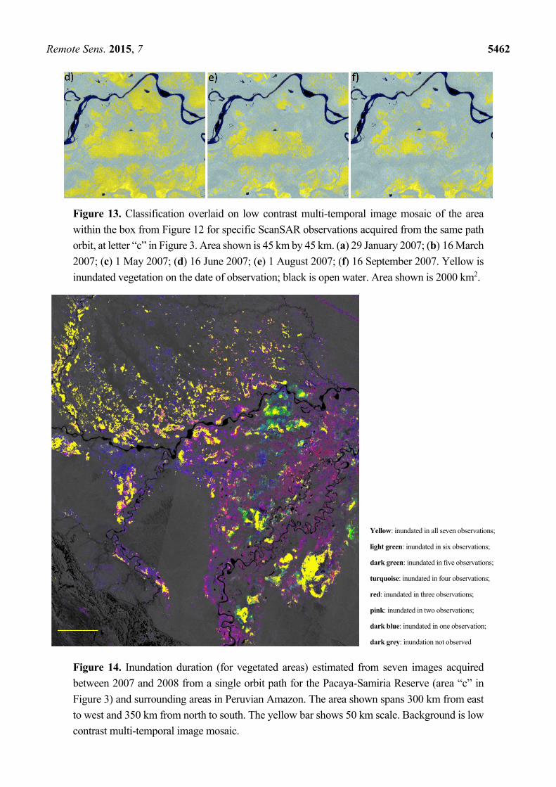
Remote Sens. 2015, 7 5462
Figure 13. Classification overlaid on low contrast multi-temporal image mosaic of the area
within the box from Figure 12 for specific ScanSAR observations acquired from the same path
orbit, at letter “c” in Figure 3. Area shown is 45 km by 45 km. (a) 29 January 2007; (b) 16 March
2007; (c) 1 May 2007; (d) 16 June 2007; (e) 1 August 2007; (f) 16 September 2007. Yellow is
inundated vegetation on the date of observation; black is open water. Area shown is 2000 km2.
Yellow: inundated in all seven observations;
light green: inundated in six observations;
dark green: inundated in five observations;
turquoise: inundated in four observations;
red: inundated in three observations;
pink: inundated in two observations;
dark blue: inundated in one observation;
dark grey: inundation not observed
Figure 14. Inundation duration (for vegetated areas) estimated from seven images acquired
between 2007 and 2008 from a single orbit path for the Pacaya-Samiria Reserve (area “c” in
Figure 3) and surrounding areas in Peruvian Amazon. The area shown spans 300 km from east
to west and 350 km from north to south. The yellow bar shows 50 km scale. Background is low
contrast multi-temporal image mosaic.

Remote Sens. 2015, 7 5463
Table 8. Area of each category of relative inundation duration (i.e., number of dates
inundated). Colors correspond with those shown in Figure 14.
Relative Inundation Duration Area
7 (Yellow) 6939 km2
6 (Light Green) 540 km2
5 (Dark Green) 911 km2
4 (Turquoise) 1715 km2
3 (Red) 2952 km2
2 (Pink) 4778 km2
1 (Dark Blue) 8237 km2
3.3. Comparison with Coarse Resolution Surface Water Fraction Estimates
Finally, we compared wetland classifications generated from high resolution ALOS PALSAR data
with that generated from much lower resolution (but much shorter orbit repeat intervals of three days or
less) spaceborne sensors such as AMSR-E, which is a passive microwave radiometer. The coarse
resolution surface water fraction product from these sensors was generated globally and aggregated to
10-day intervals. Each 25 × 25 km grid cell represented fractional surface water area. The AMSR-E
inundation product used herein was that of Schroeder et al. [45], extended to all snow-free days from
July 2002 through July 2009 [46].
To facilitate this comparison, we generated a 25 km pixel-spacing fractional open water map and a
25 km pixel-spacing fractional inundated vegetation map from our maximum and minimum inundation
classifications derived from ALOS ScanSAR data (refer to Figure 7). Likewise, we examined
the 10-day coarse resolution surface water fraction product for the time span roughly corresponding to
the ALOS acquisitions (November 2006 to July 2009) and produced a maximum and minimum surface
water fraction product. As can be seen from Figure 15, the coarse resolution surface water fraction most
closely agreed with the fraction of open water estimated from ALOS ScanSAR, rather than the fraction
of inundated vegetation, perhaps because the coarse resolution sensors are less sensitive to water beneath
a vegetation canopy. We found qualitative agreement between the coarse resolution surface water
fraction and the ALOS derived open-water fraction at both maximum and minimum inundation.
In general, we found that the maximum coarse resolution surface water fraction was slightly less than
or similar to the ALOS maximum open water fraction, except in the northwestern and southeastern
quadrants of the mapped area and along major rivers, where the maximum ALOS open water fraction
was substantially greater. These open water areas are regions where seasonal flooding can occur and are
either being overestimated by the ALOS ScanSAR classification or underestimated by the coarse
resolution surface water fraction product. Since it is likely water depth is quite shallow in these areas, it
could be a matter of the definition of what constitutes “open water;” the ScanSAR data are sensitive to
shallow but widespread flooding, but the coarse resolution product requires a noticeable change in
measured emissivity by AMSR-E. It also may be that bare soil or low vegetation associated with
agriculture or ranching in these areas has backscatter values as low as open water. The ALOS ScanSAR
classification results over agricultural areas and ranchlands present in some of these areas, and not masked
by ESA’s GlobCover land cover classification product, may account for part of the discrepancy, as well
as desert areas to the west of the Andes where the dark radar returns are similar to those for open water.

Remote Sens. 2015, 7 5464
Figure 15. Comparison of inundation and coarse-resolution surface water fraction products
for the same area shown in Figure 3. (a) Minimum fraction of open water from ALOS
ScanSAR classification; (b) minimum fractional surface water area from coarse resolution
sensors; (c) minimum fraction of inundated vegetation from ALOS ScanSAR classification;
(d) maximum fraction of open water from ALOS ScanSAR classification; (e) maximum
fractional surface water area from coarse resolution sensors; (f) maximum fraction of
inundated vegetation from ALOS ScanSAR classification. Blue indicates masked pixels;
grey scale indicates relative fractional inundation with white indicating maximum surface
water fraction and black indicating no inundation.
We examined the relationship of these coarse resolution surface water fraction data sets to each other
quantitatively. Figure 16 shows, within the JERS-1 image mosaic region area, plots of the maximum ALOS
open water fraction, the maximum ALOS inundated vegetation fraction, and the JERS-1 based wetland
fractional mask versus the maximum coarse resolution surface water fraction, aggregated for every 1°
by 1° in latitude and longitude. We found that, in general, there was close to a one-to-one relation between
ALOS open water fraction and the coarse resolution surface water fraction (slope = 0.89), but the maximum
inundated vegetation fraction and JERS-1 based wetland mask showed a significant divergence from a
one-to-one slope. Note that by choosing the JERS-1 image mosaic area, we excluded the areas where the
values diverge. This not only demonstrates the correspondence of SAR classification of open water extent
to coarse resolution inundation fraction products such as that derived by AMSR-E, but also the need for
L-band products for monitoring inundation beneath forest canopies.

Remote Sens. 2015, 7 5465
Figure 16. Comparison of ALOS and JERS-1 products with coarse-resolution surface water
fraction. (a) ALOS open water fraction; (b) ALOS inundated vegetation fraction;
(c) JERS-1-based mask (where there is overlap) versus the coarse resolution surface water
fraction. Note that the scale of (c) is much larger. Only the ALOS open water fraction has
a significant relation to the coarse resolution surface water fraction estimates.
(a)
(b)
(c)

Remote Sens. 2015, 7 5466
4. Conclusions
The objectives of this work were to assemble and mosaic JAXA L-band ALOS PALSAR ScanSAR
imagery for analysis of wetland dynamics at continental scales, then use existing algorithms for
identifying inundation, both open water extent and inundated vegetation extent. The ALOS PALSAR
ScanSAR data obtained through JAXA’s ALOS Kyoto and Carbon Initiative, in coordination with a
NASA MEASURES task to produce an Earth Science Data Record (ESDR), have been used to classify
inundation state for all of South America north of 24°S latitude.
With properly orthorectified and calibrated data, we found, as expected, that the radar signatures for
inundated vegetation and open water were easily identified. Classification parameters were assigned
from published criteria derived from extensive field measurements, together with a multi-temporal
analysis of backscatter change.
We compared the ALOS ScanSAR classification results at maximum and minimum inundation state
with a JERS-1 based wetland classification. We also compared results against a JERS-1 based wetland
mask that identified inundatable area. Our results showed that the ALOS ScanSAR classification of
inundated vegetation was relatively insensitive to inundated herbaceous vegetation. Polarimetric L-band
SAR observations, or additional observations at a shorter wavelength, may improve the capability of
future spaceborne SAR missions to detect these marshes.
The existence of an inundatable mask significantly improved the likelihood of a correct classification,
as it eliminated areas unlikely to be inundated; some of the areas eliminated may have radar signatures
similar to those from inundation events. An inland inundatable mask, based on data sources such as
SRTM (for examining slope) and products like GlobCover, could be constructed to include all known
inland floodplains, rivers, and lakes, but exclude urban areas, most desert areas, most agricultural areas,
volcanic lava flows, ocean boundaries, and areas of large slopes. Using such a mask, even if
it overrepresented the inundatable area, would significantly improve the classification accuracy by
excluding those areas that are unlikely to be inundated.
Inundation dynamics were examined using the multi-temporal ALOS ScanSAR acquisitions over
the Pacaya-Samiria and surrounding areas in the Western Amazon lowlands of Peru. Relative
inundation duration was estimated, revealing distinct local variations likely associated with differing
swamp characteristics.
Lastly, we compared inundation results from the ALOS multi-temporal ScanSAR classification with
independent results from the coarse resolution sensor AMSR-E, acquired during the same time period.
Good correspondence was found when comparing open water extent with surface water fraction, except
in regions where there may be differences in sensitivity to widespread and shallow seasonal flooding
events, or in areas that would be masked out from analysis if a continental scale inundatable mask was
available, one conceptually similar to the JERS-1 based wetland mask for the lowland Amazon.
These results compose a portion of an Inundated Wetlands Earth Science Data Record (IW-ESDR)
funded by NASA’s MEaSUREs program. Through this program, these data products are made available
through the ASF wetlands portal at the Alaska Satellite Facility Data Active Archive Center (ASF
DAAC) [47].
Further study is required to fully understand the uncertainties in these results; in particular, polarimetric
and interferometric L-band SAR data such as will be collected on a wide scale by the JAXA ALOS-2

Remote Sens. 2015, 7 5467
L-band SAR mission and the forthcoming NASA/ISRO L-band SAR mission, will be capable of
enhanced monitoring of large-scale wetland dynamics. Validation using HH and HV over a broad range
of incidence angles and incorporating zero-baseline interferometric results to identify inundation state
have not yet been conducted over globally representative regions.
Acknowledgments
We thank the NASA MEaSUREs program and Martha Maiden for funding this work, the
NASDA/JAXA GRFM project for the JERS-1 imagery, the Alaska Satellite Facility ALOS Data node
for ancillary ALOS data, the global classification from ESA’s GlobClover land cover classification
product, and the NASA SRTM project for its near global DEM. This research was undertaken within
the framework of the ALOS Kyoto & Carbon Initiative. The ALOS data were provided by JAXA EORC.
Resources supporting this work were provided by the NASA High-End Computing (HEC) Program
through the NASA Advanced Supercomputing (NAS) Division at Ames Research Center. We also thank
the editor and the reviewers for their advice and suggestions for the improvement of this paper.
This work was partially performed at the Jet Propulsion Laboratory, California Institute of Technology,
under contract with the National Aeronautics and Space Administration. U.S. Government
sponsorship acknowledged.
Author Contributions
B.C. wrote the paper, created the figures, produced the SAR image products and inundation products,
and analyzed statistics for the products and product comparisons. K.M. led the development of the
concept for the inundated wetlands earth science data record, was actively involved in acquisition
planning for the SAR data, and oversaw the development of the inundation fraction product. R.S.
developed the inundation fraction and assisted in the interpretation of this data relative to this work. A.R.
developed the observation scenario for the data acquisition and the conception of the wetlands theme for
the ALOS Kyoto and Carbon Initiative. M.S. developed the path image products that were used to
produce the image products used here. He was also actively involved in the acquisition strategy to obtain the data. L.H. contributed to the development of the concept for the inundated wetlands earth science
data record, was actively involved in acquisition planning for the SAR data, and contributed validation
maps and their interpretation relative to this work.
Conflicts of Interest
The authors declare no conflict of interest.
References
1. Hess, L.L.; Melack, J.M.; Novo, E.M.L.M.; Barbosa, C.C.F.; Gastil, M. Dual-season mapping of
wetland inundation and vegetation for the central Amazon region. Remote Sens. Environ. 2003,
87, 404–428.

Remote Sens. 2015, 7 5468
2. Hess, L.L.; Melack, J.M.; Filoso, S.; Wang, Y. Delineation of inundated area and vegetation along
the Amazon floodplain with the SIR-C synthetic aperture radar. IEEE Trans. Geosci. Remote Sens.
1995, 33, 896–904.
3. Richey, J.E.; Melack, J.M.; Aufdenkampe, A.K.; Ballester, V.M.; Hess, L.L. Outgassing from
Amazonian rivers and wetlands as a large tropical source of atmospheric CO2. Nature 2002,
416, 617–620.
4. Melack, J.M.; Hess, L.L. Remote sensing of the distribution and extent of wetlands in the Amazon
basin. In Amazonian Floodplain Forests: Ecophysiology, Ecology, Biodiversity and Sustainable
Management; Junk, W.J., Piedade, M., Wittmann, F., Schöngart, J., Parolin, P., Eds.; Springer: New
York, NY, USA, 2011; pp. 43–59.
5. Melton, J.R.; Wania, R.; Hodson, E.L.; Poulter, B.; Ringeval, B.; Spahni, R.; Bohn, T.; Avis, C.A.;
Beerling, D.J.; Chen, G.; et al. Present state of global wetland extent and wetland methane
modeling: conclusions from a model inter-comparison project. Biogeosciences 2013, 10, 753–788.
6. Cox, P.M.; Betts1, R.A.; Collins, M.; Harris, P.P.; Huntingford, C.; Jon, C.D. Amazonian forest
dieback under climate-carbon cycle projections for the 21st century. Theor. Appl. Climatol. 2004,
78, 137–156.
7. Huntingford, C.; Fisher, R.A.; Mercado, L.; Booth, B.; Sitch, S.; Harris, P.P.; Cox, P.M.;
Jones, C.D.; Betts, R.A.; Malhi, Y.; et al. Towards quantifying uncertainty in predictions of
Amazon “dieback”. Phil. Trans. R. Soc. B 2008, doi:10.1098/rstb.2007.0028.
8. Lenton, T.M.; Held, H.; Kriegler, E.; Hall, J.W.; Lucht, W.; Rahmstorf, S.; Schellnhuber, H.J.
Tipping elements in the Earth’s climate system. Proc. Natl. Acad. Sci. USA 2008, 105, 1786–1793.
9. Smith, L.C. Satellite remote sensing of river inundation area, stage, and discharge: A review.
Hydrol. Process. 1997, 11, 1427–1439.
10. Vanderbilt, V.C.; Perry, G.L.; Livingston, G.P.; Ustin, S.L.; Barrios, M.C.D.; Bréon, F.-M.;
Leroy, M.M.; Balois, J.-Y.; Morrissey, L.A.; Shewchuk, S.R.; et al. Inundation discriminated using
sun glint. IEEE Trans. Geosci. Remote Sens. 2002, 40, 1279–1287.
11. Prigent, C.; Papa, F.; Aires, F.; Rossow, W.B.; Matthews, E. Global inundation dynamics inferred
from multiple satellite observations, 1993–2000. J. Geophys. Res. 2007, 112, D12107.
12. Alsdorf, D.; Han, S.-C.; Bates, P.; Melack, J. Seasonal water storage on the Amazon floodplain
measured from satellites. Remote Sens. Environ. 2010, 114, 2448–2456.
13. Lee, H.R.; Beighley, E.; Alsdorf, D.; Jung, H.C.; Shum, C.K.; Duan, J.; Guo, J.; Yamazak, D.;
Andreadis, K. Characterization of terrestrial water dynamics in the Congo Basin using GRACE and
satellite radar altimetry. Remote Sens. Environ. 2011, 115, 3530–3538.
14. Hess, L.L.; Melack, J.M.; Simonett, D.S. Radar detection of flooding beneath the forest canopy:
A review. Int. J. Remote Sens. 1990, 11, 1313–1325.
15. Kasischke, E.S.; Bourgeau-Chavez, L.L. Monitoring South Florida wetlands using ERS-1 SAR
imagery. Photogramm. Eng. Remote Sens. 1997, 33, 281–291.
16. Kasischke, E.S.; Smith, K.B.; Bourgeau-Chavez, L.L.; Romanowicz, E.A.; Brunzell, S.;
Richardson, C.J. Effects of seasonal hydrologic patterns in South Florida wetlands on radar
backscatter measured from ERS-2 SAR imagery. Remote Sens. Environ. 2003, 88, 423–441.

Remote Sens. 2015, 7 5469
17. Frappart, F.; Seyler, F.; Martinez, J.-M.; Leon, J.G.; Cazenave, A. Floodplain water storage in the
Negro River basin estimated from microwave remote sensing of inundation area and water levels.
Remote Sens. Environ. 2005, 99, 387–399.
18. Arnesen, A.S.; Silva, T.S.F.; Hess, L.L.; Novo, E.M.L.M.; Rudorff, C.M.; Chapman, B.D.;
McDonald, K.C. Monitoring flood extent in the lower Amazon River floodplain using
ALOS/PALSAR ScanSAR images. Remote Sens. Environ. 2013, 130, 51–61.
19. Rosenqvist, A.; Shimada, M.; Chapman, B.; Freeman, A.; De Grandi, G.; Saatchi, S.; Rauste, Y.
The Global Rain Forest Mapping project—A review. Int. J. Remote Sens. 2000, 21, 1375–1387.
20. Farr, T.G.; Rosen, P.A.; Caro, E.; Crippen, R.; Duren, R.; Hensley, S.; Kobrick, M.; Paller, M.;
Rodriguez, E.; Roth, L.; et al. The Shuttle Radar Topography Mission. Rev. Geophys. 2007, 45,
doi:10.1029/2005RG000183.
21. NASA Ames Advanced Supercomputing Division. Available online: http://www.nas.nasa.gov
(accessed on 15 April 2014).
22. Rosenqvist, A.; Shimada, M.; Ito, N.; Watanabe, M. ALOS PALSAR: A pathfinder mission for
global-scale monitoring of the environment. IEEE Trans. Geosci. Remote Sens. 2007, 45, 3307–3316.
23. Rosenqvist, A.; Shimada, M.; Watanabe, M. ALOS PALSAR: Technical outline and mission
concepts. In Proceedings of the 4th International Symposium on Retrieval of Bio- and Geophysical
Parameters from SAR Data for Land Applications, Innsbruck, Austria, 16–19 November 2004.
24. Shuttle Radar Topography Mission. Available online: http://www2.jpl.nasa.gov/srtm (accessed on
22 January 2015).
25. Rodriguez, E.; Morris, C.S.; Belz, J.E.; Chapin, E.C.; Martin, J.M.; Daffer, W.; Hensley, S.
An Assessment of the SRTM Topographic Products; Technical Report JPL D-31639; Jet Propulsion
Laboratory: Pasadena, CA, USA, 2005; p. 143.
26. Rosenqvist, A.; Shimada, M.; Chapman, B.; McDonald, K.; De Grandi, G.; Jonsson, H.; Williams, C.;
Rauste, Y.; Nilsson, M.; Sango, D.; et al. An overview of the JERS-1 SAR Global Boreal Forest
Mapping (GBFM) project. In Proceedings of the 2004 IEEE International Symposium on Geoscience
and Remote Sensing (IGARSS’04), Anchorage, AK, USA, 20–24 September 2004.
27. Kawanishi, T.; Sezai, T.; Ito, Y.; Imaoka, K.; Takeshima, T.; Ishido, Y.; Shibata, A.; Miura, M.;
Inahata, H.; Spencer, R.W. The Advanced Microwave Scanning Radiometer for the Earth
Observing System (AMSR-E), NASDA’s contribution to the EOS for global energy and water cycle
studies. IEEE Trans. Geosci. Remote Sens. 2003, 41, 184–194.
28. NOAA Office of Satellite and Product Operations. Available online: http://www.ospo.noaa.gov/
Products/land/smops/sensors_AMSRE.html (accessed on 22 January 2015).
29. Ulander, L.M.H. Radiometric slope correction of synthetic-aperture radar images. IEEE Trans.
Geosci. Remote Sens. 1996, 34, 1115–1122.
30. Shimada, M.; Isoguchi, O. JERS-1 SAR mosaics of Southeast Asia using calibrated path images.
Int. J. Remote Sens. 2002, 23, 1507–1526.
31. Werner, C.; Wegmüller, U.; Strozzi, T.; Wiesmann, A. Gamma SAR and interferometric processing
software. In Proceedings of the ERS-ENVISAT Symposium, Gothenburg, Sweden, 16–20 October
2000.
32. Gabriel, A.K.; Goldstein, R.M. Crossed orbit interferometry: Theory and experimental results from
SIR-B. Int. J. Remote Sens. 1988, 9, 857–872.

Remote Sens. 2015, 7 5470
33. Shimada, M. Ortho-rectification and slope correction of SAR data using DEM and its accuracy
evaluation. IEEE J. Sel. Top. Appl. Earth Obs. Remote Sens. 2010, 3, 657–671.
34. Lucas, R.; Armston, J.; Fairfax, R.; Fensham, R.; Accad, A.; Carreiras, J.; Kelley, J.; Bunting, P.;
Clewley, D.; Bray, S.; et al. An evaluation of the ALOS PALSAR L-band backscatter—Aboveground
biomass relationship Queensland, Australia: Impacts of surface moisture condition and vegetation
structure. IEEE J. Sel. Top. Appl. Earth Obs. Remote Sens. 2010, 3, 576–593.
35. Martinez, J.-M.; Thuy Le, T. Mapping of flood dynamics and spatial distribution of vegetation in
the Amazon floodplain using multitemporal SAR data. Remote Sens. Environ. 2007, 108, 209–223.
36. Telmer, K.H.; Costa, M.P.F. SAR-based estimates of the size distribution of lakes in Brazil and
Canada: A tool for investigating carbon in lakes. Aquat. Conserv. Mar. Freshw. Ecosyst. 2007, 17,
289–304.
37. ESA GlobCover. Available online: http://due.esrin.esa.int/globcover (accessed on 15 April 2014).
38. LPDAAC. NASA Shuttle Radar Topography Mission Water Body Data Shapefiles & Raster Files.
Available online: https://lpdaac.usgs.gov/products/measures_products_table/srtmswbd (accessed
on 22 January 2015).
39. Chapman, B.; Siqueira, P.; Freeman, A. The JERS Amazon Multi-Season Mapping Study (JAMMS):
Observation strategies and data characteristics. Int. J. Remote Sens. 2002, 23, 1427–1446.
40. Siqueira, P.; Chapman, B.; McGarragh, G. The creation and interpretation of the multiseason
JERS-1 SAR mosaic over South America. Remote Sens. Environ. 2003, 87, 389–403.
41. Chapman, B.; Taylor, V.; Rosenqvist, A. Rain Forest Mapping Project to release CD-ROMs.
EOS Trans. Am. Geophys. Union 1998, 79, 417.
42. Yongwei, S.; Alsdorf, D.E. Automated georeferencing and orthorectification of Amazon basin-wide
SAR mosaics using SRTM DEM data. IEEE Trans. Geosci. Remote Sens. 2005, 43, 1929–1940.
43. Zhang, L.; Wu, W.; Zhou, Q.; Chen, Z.; Li, Z. Assess the accuracy of the Globcover cultivated land
data in Northeast China. In Proceedings of the 2012 First International Conference on
Agro-Geoinformatics (Agro-Geoinformatics), Shanghai, China, 2–4 August 2012.
44. Kalliola, R.; Puhakka, M.; Salo, J.; Tuomisto, H.; Ruokolainen, K. The dynamics, distribution and
classification of swamp vegetation in Peruvian Amazonia. Ann. Bot. Fenn. 1991, 28, 225–239.
45. Schroeder, R.; Rawlins, M.; McDonald, K.C.; Podest, E.; Zimmermann, R.; Kueppers, M. Satellite
microwave remote sensing of North Eurasian inundation dynamics: Development of
coarse-resolution products and comparison with high-resolution synthetic aperture radar data.
Environ. Res. Lett. 2010, 5, 015003.
46. JPL Wetlands Website. Available online: http://wetlands.jpl.nasa.gov (accessed on 8 May 2014).
47. ASF Wetlands Portal. Available online: https://portal.asf.alaska.edu/wetlands (accessed on 8
May 2014).
© 2015 by the authors; licensee MDPI, Basel, Switzerland. This article is an open access article
distributed under the terms and conditions of the Creative Commons Attribution license
(http://creativecommons.org/licenses/by/3.0/).