spaceborne synthetic aperture radar (sar) applications in marine meteorology xiaofeng li noaa/nesdis...
TRANSCRIPT

Spaceborne synthetic aperture radar (SAR) applications in marine meteorology
Xiaofeng Li
NOAA/NESDIS
AcknowledgmentZheng Weizhong and William Pichel, NOAA/NESDISXiaofeng Yang, Institute of Remote Sensing Application, CAS
NOAA Gilmore Creek Ground Station, Alaska

Outline
Motivation
SAR Observation and WRF model simulation of Marine Atmospheric Boundary Layer (MABL) phenomena
1) Atmospheric Gravity Waves
2) Atmospheric Vortex Streets
3) Katabatic Winds
4) Storm pattern
Summary

Motivation
SAR Provides high resolution (tens to hundreds m) all day/night synoptic observation of ocean surface.
Community weather model now provides time series of sub-km actual atmospheric circulation fields.
Synergy of the two to understand the actual atmospheric conditions that leadTo the generation and evolution of these phenomena in the MABL.
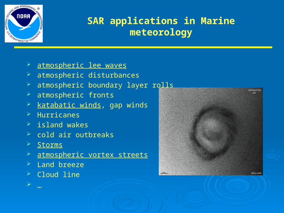
SAR applications in Marine meteorology
atmospheric lee waves atmospheric disturbances atmospheric boundary layer rolls atmospheric fronts katabatic winds, gap winds Hurricanes island wakes cold air outbreaks Storms atmospheric vortex streets Land breeze Cloud line …

1. Atmospheric Gravity Wave Observations
Upstream Waves: Waves propagates against the mean flow
Lee wave has two types of wave patterns:
1. the transverse wave type where the wave crests are nearly perpendicular to the wind direction
2. (2) the diverging wave type where the wave crests are orientated outwards from the center of the wake.

Upstream waves
1. Atmospheric Gravity Wave Observations

Upstream waves (2)
Wind variations are between 8 (wave trough)and 16 m/s (wave crest).
1. Atmospheric Gravity Wave Observations

Upstream waves 3
06/06/2001@COPYRIGHT CSA
1. Atmospheric Gravity Wave Observations
The number of wave crests increases from 3 to 8 in 4.5 hrs.

Upstream AGW can be understood by solving the FeKdV Model with Froude number f=1.1 Li, et al. 2004, JGR
1. Atmospheric Gravity Wave Observations

A RADARSAT ScanSAR wide B SAR Western AlaskaImage center (60N, 145W) 03:10:05 GMT, June 12, 2001.
(© Canadian Space Agency, 2001)
Win
d Dire
ction
Lee Wave (transverse waves)
1. Atmospheric Gravity Wave Observations

RADARSAT ScanSAR wide image shows the island lee wave pattern in the Gulf of Alaska.
• Image center: (55N, 154W) • Time16:29:42 UTC, June 27,
1997. (© CSA, 1997)
Wind Direction
Lee Wave (Diverging waves)
1. Atmospheric Gravity Wave Observations

Lee Wave (diverging waves, Example 2)W
ind
Dire
ctio
n
Constant lee wave phase linesChunchuzov, Vachon, and Li, Remote Sensing of Environment, 74, 343-361, 2000.
1. Atmospheric Gravity Wave Observations

1. Atmospheric Gravity Wave Observations
Lee Wave 3

Lee wave simulation with WRFWeather Research and ForecastingNCAR Community modelTwo-way nested domains:D1: 9km 280 x 251D2: 3km 310 x 301D3: 1km 271 x 262Vertical levels: 27
Model parameterization: • Rapid Radiative Transfer Model (RRTM) longwave
radiation • Dudhia shortwave radiation• Yonsei University (YSU) planetary boundary layer
scheme• WRF Single Moment 3‐Class (WSM)
cloudmicrophysics, • Kain‐Fritsch (new Eta) convective
parameterization employed only in coarse and medium domains,
• Monin‐Obukhov surface‐layer scheme• Noah land‐surface model.
Boundary conditions are specified by linearly interpolating the NCEP 6 hourly final analyses (FNL) at a resolution of 1° × 1° degree.
The digital elevation of 30 s USGS topography data.
1. Atmospheric Gravity Wave Observations

1. Atmospheric Gravity Wave Observations
WRF Simulation results at the imaging time
Vertical velocity
Horizontal velocity

1. Atmospheric Gravity Wave Observations
Standing WavesMODIS true color image acquired about 8.5 h prior to the Envisat ASAR pass in Google Earth.
Lee Wave 3

1. Atmospheric Gravity Wave Observations
Lee Wave 4
Not trapped in the MABL

1. Atmospheric Gravity Wave Observations
Lee Wave 4
Comparison of WRF simulated surface wind speed with the independent SAR measurements

AGW Summary
AGM patterns can be identified on SAR image.
Most of the waves generated by flow over bump observed by SAR are on the lee side of the bump, and has two types of wave patterns.
The terrain-forced stmospheric lee waves can be simulated using the WRF model. Model reveals evolution of the AGW.
Upstream waves happen when Froude number is close to 1. They are elevation waves. They are explained well with FeKDV model.
1. Atmospheric Gravity Wave Observations

2. Atmospheric Vortex Streets (AVS)
Atmospheric vortex-street patterns on the lee side of a flow obstacle double row of counter rotating vortex pairs shedding alternately near the
edge of the obstacle No observation in the atmosphere prior to the satellite age due to AVS
scale (100-400 km): too small to be delineated by a synoptic observation network and too large to be observed by a single station
h/a is the basic property of an atmospheric vortex streets Uo is the wind speed, Ue is the vortex shedding velocity

NASA space shuttle picture cloud pattern (1)
NASA space shuttle picture cloud pattern (2)
2. Atmospheric Vortex Streets (AVS)

Landsat-7 (Defelice et al. Vol. 81,No.5, 1047-1048, BAMS, 2000)-cloud
pattern
Aircraft photo (Ferrier et al. Vol. 17,
No. 1, 1-8, International J. of Remote
Sensing, 1996)- sediment pattern
SAR Wind Pattern. IEEE/TGARSSFeb. 2004
2. Atmospheric Vortex Streets (AVS)

ATMOSPHERIC VORTEX STREETS OBSERVED ON
REMOTE SENSING IMAGES (3)
RADARSAT synthetic aperture radar (SAR) image (© CSA, 1999)
RADARSAT synthetic aperture radar (SAR) image (© CSA, 1999)
Li, et al. 2002, GRL

SAR observation of AVS
Li, et al. 2008, Sensors
2. Atmospheric Vortex Streets (AVS)

WRF Simulation of AVS
Li, et al. 2008, Sensors
2. Atmospheric Vortex Streets (AVS)

WRF Simulation of AVS
• Vortex shedding rate and propagation velocity
•Reynolds Number (50-250)
•Frude Number (0.15-0.4)
•Vorticity and energy dissipation
2. Atmospheric Vortex Streets (AVS)

3. Katabatic Wind
katabatic wind is a gravitational air flow that descends from a high-elevation mountain down slope to lower elevation.
Happens night and early morning hours in the winter season when the air mass over the mountain top becomes colder and heavier due to fast radiation cooling and when the land-sea temperature gradient is large.

3. Katabatic Wind
hourly coastal horizontal wind speed

3. Katabatic Wind
The black solid line is the topography; the red dash line represents the horizontal wind speed simulated by the model, the blue line represents the sea surface wind derived from SAR measurements, and the green dash line represents the near surface descending wind speed

3. Katabatic Wind
• Summary:
• The wind associated with the katabatic wind varies between 5 and 8 m/s
• The katabatic wind finger extends up to 20 km offshore.
• The 3-layer nested weather model simulation captures the finger-like katabatic wind pattern
observed in the SAR image.
• Katabatic wind is the strongest at 14:00 UTC when the land-sea temperature gradient is the
largest.
• The low-level model wind speed is very close to that derived from the SAR image.
• The SAR image shows a more detailed finger-like katabatic wind structure than that shown in the
• model simulation.

4 Storm and Precipitation

4 Storm and Precipitation

4 Storm and Precipitation

4 Storm and Precipitation
Storm Summary:
WRF can capture wind and rain pattern in the storm
Heavy rain in the hurricanes damps NRCS.
Moderate rain has less effect in C-band NRCS than wind does in the regular storm case

5 Summary
We have set up WRF model to simulate SAR observed MABL phenomena
WRF model captures the basic characteristics AGV, AVS, Katabatic and Storm
The 1-km resolution WRF model gives detailed structures of the phenomena
This leads to the understanding of generation and evolution of these phenomena
Synergy of SAR and WFR provides great opportunity for detailed study of MABLPhenomena