mapping north african landforms using continental scale ... · mapping north african landforms...
TRANSCRIPT
www.elsevier.com/locate/rse
Remote Sensing of Environm
Mapping North African landforms using continental scale unmixing
of MODIS imagery
John-Andrew C. Ballantine a,*, Gregory S. Okin b, Dylan E. Prentiss a, Dar A. Roberts a
aDepartment of Geography, University of California Santa Barbara, EH3611, Santa Barbara, CA 93106, USAbDepartment of Environmental Sciences, University of Virginia, Charlottesville, VA 22904-4123, USA
Received 14 December 2004; received in revised form 25 April 2005; accepted 29 April 2005
Abstract
We describe the production of a landform map of North Africa utilizing moderate resolution satellite imagery and a methodology that
is applicable for sub-continental to global scale landform mapping. A mosaic of Moderate Resolution Imaging Spectroradiometer
(MODIS) apparent surface reflectance imagery was compiled for Africa north of 10- N. Landform image endmembers were chosen to
characterize ten different types of vegetated and unvegetated desert surfaces: alluvial complexes, dunes, dry and ephemeral lakes, open
water, basaltic volcanoes and flows, mountains, regs, stripped, low-angle bedrock surfaces, sand sheets, and Sahelian vegetation. Multiple
Endmember Spectral Mixture Analysis (MESMA) was applied to the MODIS mosaic to estimate landform and vegetation endmember
fractions. The major landform in each MODIS pixel was identified based on the majority endmember fraction in two- or three-endmember
models. Accuracy assessment was conducted using two data sources: the historic Landform Map of North Africa [Raisz, E. (1952).
Landform Map of North Africa. Environmental Protection Branch, Office of the Quartermaster General.] and Landsat Thematic Mapper
(TM) data. Comparison with the Raisz landform map gave an overall classification accuracy of 54% with significant confusion between
alluvial surfaces and regs, and between sandy and clayey surfaces and dunes. A second validation using 20 Landsat images in a stratified
sampling scheme gave a classification accuracy of 70%, with confusion between dunes and sand sheets. Both accuracy assessment
schemes indicated difficulty in vegetation classification at the margin of the Sahel. A comparison with minimum distance and maximum
likelihood supervised classifications found that the MESMA approach produced significantly higher classification accuracies. This digital
landform map is of sufficiently high quality to form the basis for geomorphic studies, including parameterization of the surface in global
and regional dust models.
D 2005 Elsevier Inc. All rights reserved.
Keywords: Sahel; Sahara; Landform; Desert; Dust source; MESMA; Landform endmembers; Wind erosion
1. Introduction
The Sahara Desert is the largest in the world and
arguably the most diverse in terms of the range of landforms
found within it. Tucker and Nicholson (1999) found the
mean size of the Sahara Desert, between 1980 and 1997,
was 9,149,000 km2. The size of this region makes the
traditional mapping methods of aerial photography and field
surveying of limited use. Moderate resolution multispectral
0034-4257/$ - see front matter D 2005 Elsevier Inc. All rights reserved.
doi:10.1016/j.rse.2005.04.023
* Corresponding author. Tel.: +1 207 299 3703.
E-mail address: [email protected] (J.-A.C. Ballantine).
data allows continental- to global-scale mapping of the
Earth’s surface while retaining sufficient resolution for
geomorphic and ecological studies.
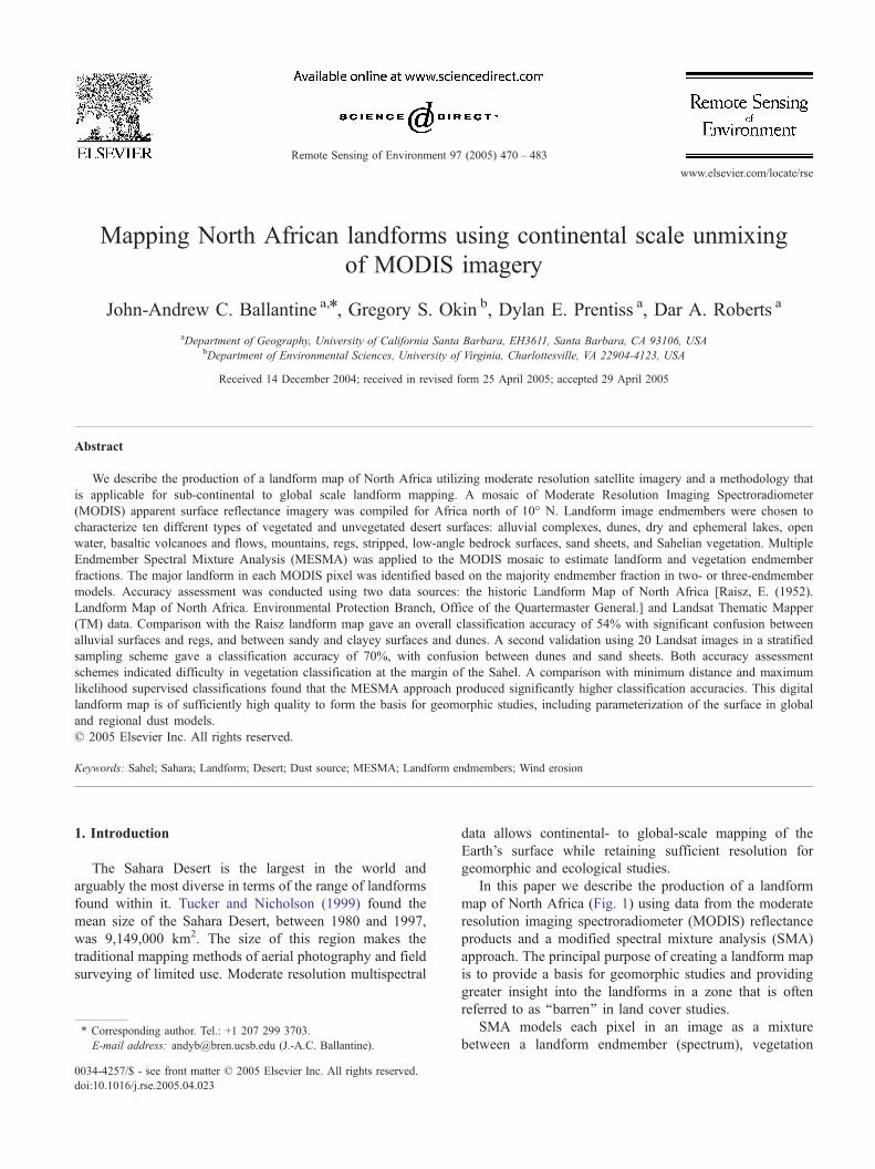
In this paper we describe the production of a landform
map of North Africa (Fig. 1) using data from the moderate
resolution imaging spectroradiometer (MODIS) reflectance
products and a modified spectral mixture analysis (SMA)
approach. The principal purpose of creating a landform map
is to provide a basis for geomorphic studies and providing
greater insight into the landforms in a zone that is often
referred to as ‘‘barren’’ in land cover studies.
SMA models each pixel in an image as a mixture
between a landform endmember (spectrum), vegetation
ent 97 (2005) 470 – 483
10oW
30oN
20oN
30oN
20oN
0oE 10oE 20oE 30oE 40oE
10oW 0oE 10oE 20oE 30oE 40oE
Lake
Study Area
Country
River
0 337.5 675 1,350 2,025 2,700Kilometers
Legend
Morocco
WesternSahara
Mauritania
Senegal
Mali
Algeria
Niger
Libya
Chad Sudan
Egypt
Tunisia
Niger River
Lake Chad
Lake Nasser
Nile River
N
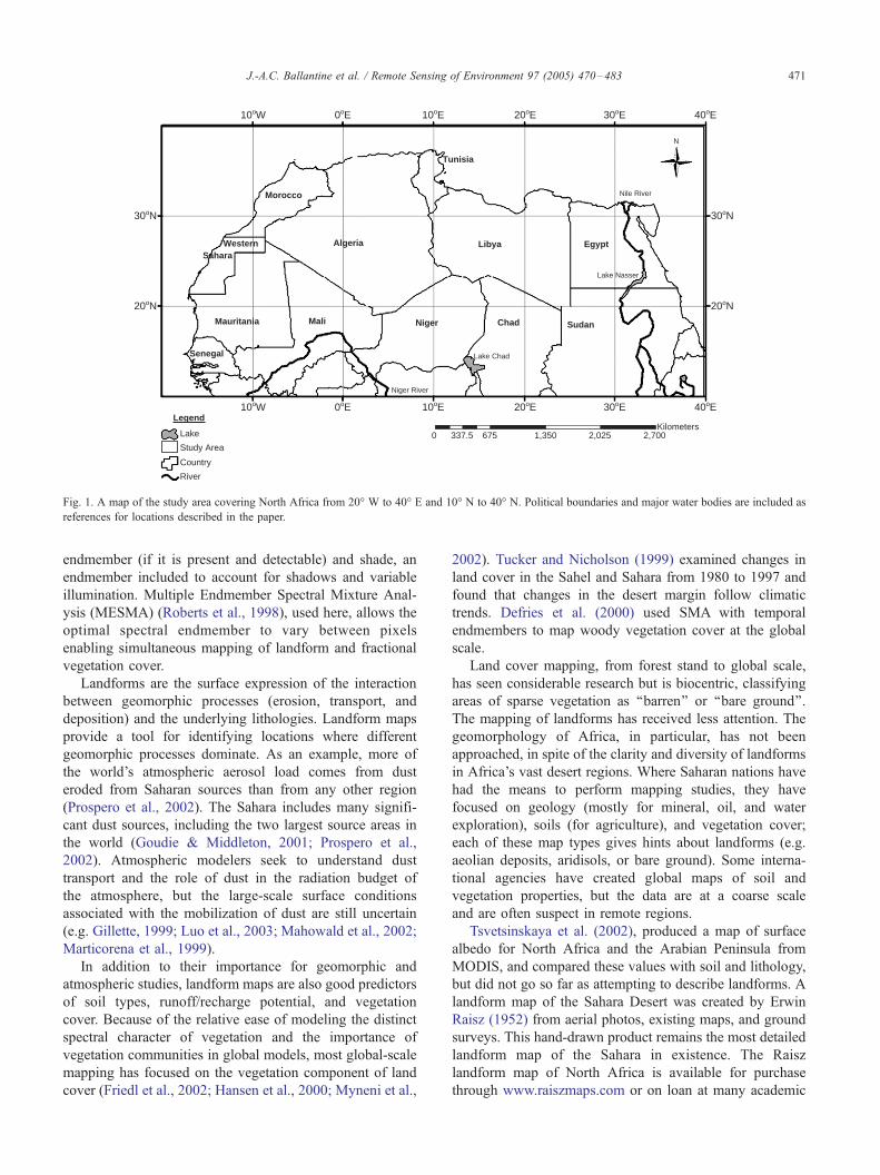
Fig. 1. A map of the study area covering North Africa from 20- W to 40- E and 10- N to 40- N. Political boundaries and major water bodies are included as
references for locations described in the paper.
J.-A.C. Ballantine et al. / Remote Sensing of Environment 97 (2005) 470–483 471
endmember (if it is present and detectable) and shade, an
endmember included to account for shadows and variable
illumination. Multiple Endmember Spectral Mixture Anal-
ysis (MESMA) (Roberts et al., 1998), used here, allows the
optimal spectral endmember to vary between pixels
enabling simultaneous mapping of landform and fractional
vegetation cover.
Landforms are the surface expression of the interaction
between geomorphic processes (erosion, transport, and
deposition) and the underlying lithologies. Landform maps
provide a tool for identifying locations where different
geomorphic processes dominate. As an example, more of
the world’s atmospheric aerosol load comes from dust
eroded from Saharan sources than from any other region
(Prospero et al., 2002). The Sahara includes many signifi-
cant dust sources, including the two largest source areas in
the world (Goudie & Middleton, 2001; Prospero et al.,
2002). Atmospheric modelers seek to understand dust
transport and the role of dust in the radiation budget of
the atmosphere, but the large-scale surface conditions
associated with the mobilization of dust are still uncertain
(e.g. Gillette, 1999; Luo et al., 2003; Mahowald et al., 2002;
Marticorena et al., 1999).
In addition to their importance for geomorphic and
atmospheric studies, landform maps are also good predictors
of soil types, runoff/recharge potential, and vegetation
cover. Because of the relative ease of modeling the distinct
spectral character of vegetation and the importance of
vegetation communities in global models, most global-scale
mapping has focused on the vegetation component of land
cover (Friedl et al., 2002; Hansen et al., 2000; Myneni et al.,
2002). Tucker and Nicholson (1999) examined changes in
land cover in the Sahel and Sahara from 1980 to 1997 and
found that changes in the desert margin follow climatic
trends. Defries et al. (2000) used SMA with temporal
endmembers to map woody vegetation cover at the global
scale.
Land cover mapping, from forest stand to global scale,
has seen considerable research but is biocentric, classifying
areas of sparse vegetation as ‘‘barren’’ or ‘‘bare ground’’.
The mapping of landforms has received less attention. The
geomorphology of Africa, in particular, has not been
approached, in spite of the clarity and diversity of landforms
in Africa’s vast desert regions. Where Saharan nations have
had the means to perform mapping studies, they have
focused on geology (mostly for mineral, oil, and water
exploration), soils (for agriculture), and vegetation cover;
each of these map types gives hints about landforms (e.g.
aeolian deposits, aridisols, or bare ground). Some interna-
tional agencies have created global maps of soil and
vegetation properties, but the data are at a coarse scale
and are often suspect in remote regions.
Tsvetsinskaya et al. (2002), produced a map of surface
albedo for North Africa and the Arabian Peninsula from
MODIS, and compared these values with soil and lithology,
but did not go so far as attempting to describe landforms. A
landform map of the Sahara Desert was created by Erwin
Raisz (1952) from aerial photos, existing maps, and ground
surveys. This hand-drawn product remains the most detailed
landform map of the Sahara in existence. The Raisz
landform map of North Africa is available for purchase
through www.raiszmaps.com or on loan at many academic

J.-A.C. Ballantine et al. / Remote Sensing of Environment 97 (2005) 470–483472
map libraries. In spite of its many qualities, the Raisz map is
an analog product of indeterminate resolution (minimum
mapping unit on the order of kilometers), and therefore
better for use as a reference than as a basis for the analysis
of landform properties. The map we produced improves on
the Raisz map in that it is reproducible, digital, and based on
a single data source. The approach used here also enables
simultaneous analysis of fractional vegetation coverage, and
thus supplements existing vegetation monitoring method-
ologies and more traditional land cover classifications.
2. Methods
2.1. Desert landforms
The Soil Science Society of America (www.soils.org)
defines a landform as ‘‘any physical, recognizable form or
feature on the earth’s surface, having a characteristic shape,
and produced by natural causes’’. One of the challenges of
creating a landform map from satellite imagery was trans-
lating from this form-based definition of landforms to a
spectral definition wherein all of the sub-pixel scale elements
of a given landform created a signature in spectral space that
could define that landform. For the purposes of this work, a
landform was considered to be a landscape element that was
spatially and spectrally distinct using 500-m resolution and
seven wavelength bands of MODIS reflectance imagery. In
cases where landforms might be spectrally confused (e.g.
dune fields and sand sheets), we attempted to distinguish
them spectrally, but also noted that many landforms with
similar spectra are also functionally similar. Ultimately,
classes where there is confusion may need to be combined or
further defined using other data sources.
Clements et al. (1957) described 10 major landforms for
the deserts of the world, including alluvial fans, sand seas,
playas, river plains, dry watercourses, mountains, recent
volcanic deposits, low-angle bedrock surfaces, desert flats,
and badlands. A similar set appears in the landform map of
Raisz (1952). Drawing on the landform classes of Raisz
and refining them to the set of landforms that may be
identified spectrally at the scale of MODIS, we identified
nine classes of landforms. These were alluvial fan systems,
dune fields, dry lakebeds, open water bodies, basaltic
volcanoes and flows, sedimentary mountain ranges, regs,
stripped bedrock surfaces, and sandsheets. Vegetated
surfaces were added as a class for areas where vegetative
cover was significant enough to obscure the underlying
landform.
The alluvial fan class includes both complexes of
alluvial fans that flank mountains and some incised plateaus.
The fan complexes are composed of unsorted sediments and
are frequently incised by ephemeral or paleo-channels.
Some alluvial systems may also have vegetation cover
because of runoff and recharge from adjacent mountains or
proximity to desert margins. The fan complexes of the
southern flank of the Atlas Mountains in Tunisia, Algeria,
and Morocco (e.g. 33.5- N, 2.5- E) are good examples of
this landform.
Ergs and dunefields are regions where sand piles into
systems of dunes or sandy plains. In the great ergs of the
central Sahara, sand dunes hundreds of meters high are
common. In relatively sediment-starved situations linear
dunes and barchan dunes with bedrock, gravel flats (regs),
or packed clayey surfaces between dunes predominate (e.g.
Thomas, 1997). In general, ergs appear bright in the MODIS
imagery. A classic dunefield example is the Erg Occidental
of Algeria (31- N, 2.5- E).Ephemeral and paleo-lakes are characterized by fine
sediments laid down by floods in recent times and/or during
previous pluvial episodes. Lake sediments have the charac-
teristic brightness of fine sediments, especially in the short-
wave infrared (SWIR) wavelengths (Okin & Painter, 2004).
The lakebed associated with paleo-lake mega-Chad in the
Bodele Basin of Chad (17- N, 18- E) is a good example of
this landform.
Open water occurs in the Sahara, associated with the
Niger and Nile Rivers, Lake Chad, Lake Nasser, and coastal
zones. Open water bodies are the darkest features in the
Sahara. As an example, Lake Nasser is located in southern
Egypt at 23.2- N, 32.8- E.Basaltic volcanoes and flows are spectrally almost as
dark as open water. Basaltic features can be found as
extensive formations in various parts of the central Sahara
such as the Black Haruj flows of Libya (27.5- N, 17.5- E).Mountain ranges in the Sahara are characterized by
uplifted sedimentary and metamorphic rocks (e.g. the
Ahaggar Mountains of Algeria, 23.2- N, 6- E). Sedimentary
and metamorphic mountain ranges appear dark in the
MODIS imagery, but not as dark as basaltic features.
Because of orographic rainfall, some vegetation can be
found in mountainous areas, even in the core of the desert.
As a result, there is a component of vegetation spectra in the
mountain landform class.
Regs or serirs may either represent deflationary land-
scapes, where aeolian activity has removed fine particles
leaving lag gravels, or accretionary landscapes, where
gravels protect underlying fine sediments from wind erosion
(e.g. McFadden et al., 1987). Whether deflationary or
accretionary, these surfaces appear darker than surfaces of
sandy or finer texture, due to the darker coloring of larger
clasts, coarser particles casting shadows, and possibly due to
the development of varnish on these particles. The Serir of
Kalansho in Libya (27.5- N, 21.5- E) typifies this landform.
Stripped bedrock includes low-angle bedrock surfaces
where erosive processes have removed the majority of the
surface regolith. These landforms may be cut by drainages or
marked by hummocky features and sinkholes in limestone
landscapes, with some sand collecting in hollows (Taylor &
Howard, 1999). Stripped bedrock surfaces are more common
in the western part of the Sahara Desert in countries such as
Mauritania and Western Sahara (23- N,13.5- W).

J.-A.C. Ballantine et al. / Remote Sensing of Environment 97 (2005) 470–483 473
Sandsheets are sedimentary plains covered in fine
sediments from loose sand to packed silt or clay. In systems
of large linear dunes, this may include the troughs between
dunes. This class is widespread with an example in Sudan at
17- N, 25- E.Vegetation is the dominant land cover in some mountain-
ous areas and in the Sahel (e.g. 17.5- N, 12.5- E). A variety
of vegetation exists in North Africa from sparse shrubs in
the arid core of the Sahara to the more densely vegetated
surfaces of the northern Sahara (e.g. Atlas plateaus, subaltic
alluvial complexes, and the Fezzan region of Libya). In the
central Sahara, more vigorous vegetation may be found in
mountainous areas (where orographic effects are strong
enough to generate rainfall), near phreatic oases, and along
the riparian zones of rivers. Vegetation has a characteristic
spectral signature and vegetation cover can be separated
from the land surface using the MESMA technique.
Although vegetation was treated as static in this study,
vegetation is a dynamic quantity, and varies in its cover
extent depending on the time of year and the amount of
rainfall during the year in question (e.g. Weiss et al., 2004).
2.2. Data collection
A mosaic of MODIS 500-meter resolution, land-surface
reflectance product (MOD09GHK) covering North Africa
from 10- N to 40- N and 20- W to 40- E was created (Fig.
2). Cloud-free imagery was chosen from the period between
November 1 and December 26, 2000. For one MODIS tile
covering Tunisia and Algeria, two images from this period
were combined to avoid clouds. These dates represent the
dry season on the southern edge of the Sahara and come
before most winter rains in the North.
2.3. MESMA
The digital landform map was created using MESMA
(Roberts et al., 1998), applied to theMODISmosaic for North
Fig. 2. A false color mosaic of MODIS MOD09GHK imagery for North Africa (R
The coverage of Landsat scenes used for validation is shown in translucent red. (Fo
referred to the web version of this article.)
Africa shown in Fig. 2. SMA typically assumes that the
reflectance of a given pixel (qVk) is composed of a linear
combination of a few ‘‘pure’’ endmember spectra (e.g. Smith et
al., 1990). Endmember spectra can be chosen from represen-
tative, homogeneous areas in the image (image endmembers)
or an existing library of reference spectra for materials
common to the image in question (reference endmembers).
qVk ¼XNi¼1
fi4qik þ ek ð1Þ
Where qik is the reflectance of endmember i in band k and fi is
the fraction of thatendmember. N is the number of endmem-
bers and ek; the residual error. Thefractions are constrained by:
XNi¼1
fi ¼ 1 ð2Þ
The fit of the endmember models can be assessed using the
root mean squarederror (RMSE) of ek:
RMSE ¼
ffiffiffiffiffiffiffiffiffiffiffiffiffiffiffiffiffiffiffiXMk¼1
ekð Þ2
M
vuuuutð3Þ
where M is the number of bands (7 for this MODIS product)
(Dennison & Roberts, 2003).
The MESMA approach differs from SMA in that the
spectrum for each pixel in the image is allowed to be
unmixed by a different set of endmembers from an overall
endmember library for the image (Roberts et al., 1998). In
our study, the MESMA technique allowed a greater
number of endmembers, representing a greater number
of surface materials, to be used. As a result, MODIS
images of widely varying surface covers were able to be
modeled based on the spectra of these surface covers. The
SMA and MESMA techniques have been described in
greater detail in Dennison and Roberts (2003) and Roberts
et al. (1998).
ed=2130 nm, Green=859 nm, Blue=555 nm). The projection is sinusoidal.
r interpretation of the references to colour in this figure legend, the reader is
J.-A.C. Ballantine et al. / Remote Sensing of Environment 97 (2005) 470–483474
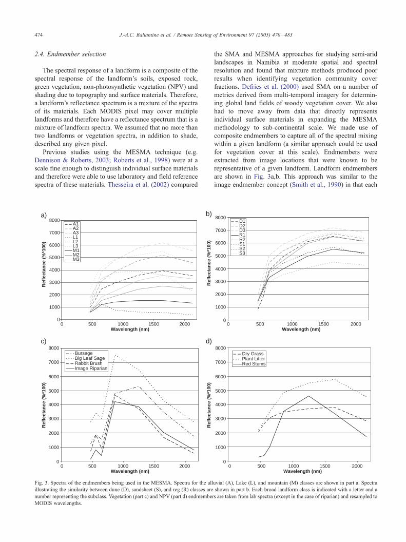
2.4. Endmember selection
The spectral response of a landform is a composite of the
spectral response of the landform’s soils, exposed rock,
green vegetation, non-photosynthetic vegetation (NPV) and
shading due to topography and surface materials. Therefore,
a landform’s reflectance spectrum is a mixture of the spectra
of its materials. Each MODIS pixel may cover multiple
landforms and therefore have a reflectance spectrum that is a
mixture of landform spectra. We assumed that no more than
two landforms or vegetation spectra, in addition to shade,
described any given pixel.
Previous studies using the MESMA technique (e.g.
Dennison & Roberts, 2003; Roberts et al., 1998) were at a
scale fine enough to distinguish individual surface materials
and therefore were able to use laboratory and field reference
spectra of these materials. Thesseira et al. (2002) compared
a)
0
1000
2000
3000
4000
5000
6000
7000
8000
0 500 1000 1500 2000Wavelength (nm)
0 500 1000 1500 2000Wavelength (nm)
Ref
lect
ance
(%
*100
)
c)
0
1000
2000
3000
4000
5000
6000
7000
8000
Ref
lect
ance
(%
*100
)
d)
Ref
lect
ance
(%
*100
)b)
Ref
lect
ance
(%
*100
)
A1A2A3L1L2L3M1M2M3
BursageBig Leaf Sage Rabbit BrushImage Riparian
Fig. 3. Spectra of the endmembers being used in the MESMA. Spectra for the all
illustrating the similarity between dune (D), sandsheet (S), and reg (R) classes are
number representing the subclass. Vegetation (part c) and NPV (part d) endmember
MODIS wavelengths.
the SMA and MESMA approaches for studying semi-arid
landscapes in Namibia at moderate spatial and spectral
resolution and found that mixture methods produced poor
results when identifying vegetation community cover
fractions. Defries et al. (2000) used SMA on a number of
metrics derived from multi-temporal imagery for determin-
ing global land fields of woody vegetation cover. We also
had to move away from data that directly represents
individual surface materials in expanding the MESMA
methodology to sub-continental scale. We made use of
composite endmembers to capture all of the spectral mixing
within a given landform (a similar approach could be used
for vegetation cover at this scale). Endmembers were
extracted from image locations that were known to be
representative of a given landform. Landform endmembers
are shown in Fig. 3a,b. This approach was similar to the
image endmember concept (Smith et al., 1990) in that each
0 500 1000 1500 2000Wavelength (nm)
0 500 1000 1500 2000Wavelength (nm)
0
1000
2000
3000
4000
5000
6000
7000
8000
0
1000
2000
3000
4000
5000
6000
7000
8000D1D2D3R1R2S1S2S3
Dry GrassPlant LitterRed Stems
uvial (A), Lake (L), and mountain (M) classes are shown in part a. Spectra
shown in part b. Each broad landform class is indicated with a letter and a
s are taken from lab spectra (except in the case of riparian) and resampled to
J.-A.C. Ballantine et al. / Remote Sensing of Environment 97 (2005) 470–483 475
landform endmember was considered to represent a pure
landform drawn from the MODIS imagery. Landform
endmembers were chosen from desert areas where vegeta-
tion cover would be minimal so as to avoid components that
would vary in time.
Because vegetation cover changes on interseasonal and
interannual time scales, while landform type is typically
stable on the order of 100s to 1000s of years, separate
endmembers for vegetation were used. Three reference NPV
(plant litter, dry grass, and red stems), three reference
vegetation (big leaf sage, rabbit brush, and bursage), and
one image vegetation endmember representing riparian
vegetation were used for vegetated regions in the image.
The vegetation and NPV spectra are shown in Fig. 3c and d,
respectively. The reference endmembers come from the
library described in Roberts et al. (1993) which is largely
composed of North American vegetation. No significant
library of Saharan and sub-Saharan vegetation was available
for this study. Although the spectra were collected from
North American sites, these spectra are broadly representa-
tive of the range of semiarid to arid NPV and vegetation
spectra. The spectral library was convolved to MODIS
wavelengths using the MODIS filter functions. Reference
endmembers were used in the case of vegetation because
vegetation was rarely the dominant endmember in a pixel
for our study area. Leafy irrigated or riparian vegetation
dominated where vegetation was the major endmember in
the pixel. Desert vegetation tends to be more sparse and
woody or grassy. It was therefore difficult to locate a ‘‘pure’’
vegetation pixel that would also represent sparse desert
vegetation. For pixels modeled by one of the vegetation
endmembers, the vegetation fraction gave an indication of
percent vegetation cover within that pixel. Using several
vegetation endmembers allowed for a range of semiarid,
riparian, and non-photosynthetic vegetation types to be
accounted for, but for the purpose of the landform map, all
of the vegetation endmembers were lumped into one
vegetation class.
One-hundred and nine endmember sites were chosen
from the MODIS mosaic using the map of Raisz (1952) as a
guide for landform type. Spectra from each of these sites
were compiled to form a spectral library of landform
endmembers for North Africa. These sites fell into six
broad landform classes (alluvial, dunes, lakes, mountains,
regs, and sandsheets) based on the classes identified in the
Raisz map. The spectra from each broad class were
statistically divided into two to three subclasses using a k-
means unsupervised cluster analysis (Funk et al., 2001). As
an example, the broad mountain class had three statistically
separate subclasses, two of which were identified as
representing mountains, and the other identified as repre-
senting basaltic volcanoes and flows.
Tompkins et al. (1997) emphasized the importance of the
selection of good spectral endmembers for any SMA.
Because of the diversity of classes in this study, we chose
the endmember average RMS (EAR) method of Dennison
and Roberts (2003) as the principal method for selecting
landform endmembers. The EAR technique selects the
endmember that is most representative of a class of
endmembers to represent that class. EAR worked well for
the broadly defined classes of this study where finding
extreme endmembers might not have represented the full
diversity of each landform class.
In order to identify the landform spectrum that was most
distinct, the spectral library of 109 landform endmembers
was unmixed by two endmember models of shade and each
of the other endmembers in the library to calculate EAR
values as described by Dennison and Roberts (2003). The
model constraints described by Dennison and Roberts were
found to work well for these data. Endmember fractions
were constrained to less than 106% with best-fit models
greater than this value being set to 106% and the RMSE
calculated from this value.
The EAR method selected an endmember representative
for a subclass by finding the endmember with the lowest
RMSE when modeling other endmembers in its subclass:
EARAi;A ¼
Xnj¼1
RMSEAi;Aj
n� 1ð4Þ
where A was the subclass, Ai was the landform endmember
in question, n was the number of spectra in subclass A, and
Aj was the spectrum being modeled by Ai. Thus, the
endmember representing basaltic flows in the Ahaggar
Mountains of Algeria was used to model the other basalt
endmembers (basalt is subclass M1 in Fig. 3a). The average
of the RMSE values from each model was the EAR value
for the Ahaggar basaltic endmember. Because the Ahaggar
basaltic endmember’s EAR value was lower than that of the
Tibesti Mountains and the other basalt endmembers, the
Ahaggar basaltic endmember was picked as the representa-
tive endmember for subclass M1. The landform spectra thus
picked are shown in Fig. 3a.
3. Modeling with MESMA
The modeling of the image with MESMA followed the
methodology of Dennison and Roberts (2003). Two-
endmember models (an endmember and shade) were run
with the constraint that non-shade fractions had to be
between �6% and 106% of the pixel. Cases where
residuals exceeded 2.5% of reflectance for more than 7
contiguous bands or RMSE exceeded 2.5% of reflectance
were left unmodeled. Similar constraints were used for
three endmember models (two endmember spectra and
shade). All possible models were considered such that
there were 24 possible two-endmember models (17 land-
form subclasses and 7 vegetation endmembers) and 276
three-endmember models. For each pixel, the lowest
RMSE two-endmember model was chosen unless the
RMSE of the three-endmember improved upon that of

Fig. 4. The shade endmember fraction image derived from the MODIS mosaic in Fig. 2. The shading bar shows % shade from �6% to 100% with values of
�100 representing bright desert surfaces with effectively no shade. Bright areas near the coast indicate deep water that has not been masked out. Note that the
shade fraction is greater on the east-side of each MODIS tile, expressing the BRDF of vegetation.
J.-A.C. Ballantine et al. / Remote Sensing of Environment 97 (2005) 470–483476
the two endmember model by more than 0.8% of
reflectance (Roberts et al., 2003).
4. Results
MESMA produced fraction images of the dominant and
secondary (in three endmember cases) endmembers, along
with the fraction of shade present. Each pixel was coded
with the classes that describe it and the fraction of each
class.
4.1. Shade fraction
In Fig. 2, it is apparent that the east side of each MODIS
tile in the mosaic is darker than the west, particularly in
vegetated regions. This occurs because the bi-directional
reflectance distribution function (BRDF) of surface materi-
als is asymmetrical with more light being back-scattered
than forward-scattered in the case of vegetation. The
variation in brightness across the tile is a function of the
amount of shadowing imaged by the sensor. An advantage
Fig. 5. The vegetation endmember fraction derived from the MODIS mosaic in Fig
of the transects shown in Fig. 6 are indicated.
of using a spectral unmixing approach is that the shade
fraction contains most of this BRDF effect. As a result, the
landform and/or vegetation endmember(s) used to determine
the landform class did not exhibit any variation due to
BRDF effects. The expression of the anisotropic BRDF of
vegetation is apparent in the shade fraction image (Fig. 4).
4.2. Vegetation fraction
The modeled vegetation endmember fraction represents
the fractional ground cover of vegetation (Fig. 5). Fig. 5
expresses the vegetation cover increase from the Sahara
south into the Sahel. Vegetation along the northern margin
of the continent is also apparent. Scattered vegetation in the
core of the Sahara is usually associated with mountain
ranges where orographic rainfall and springs make signifi-
cant vegetation viable. If multi-temporal imagery had been
used, the vegetation fraction could tracked be to show
changes in vegetation cover and its response to rainfall
variation.
The red stems vegetation endmember dominated the
scene because it best modeled Sahel vegetation (Table 1). In
. 2. The shading bar shows percent vegetation cover. Approximate locations

Table 1
Areal coverage and proportion of vegetation fractions in the Fig. 5
Class # Name Area (km2) % Vegetation
18 Dry grass 92,886.75 4.89
19 Plant litter 28,845.25 1.52
20 Red stems 1,568,183.8 82.48
21 Bursage 180.75 0.01
22 Big leaf sage 1226 0.06
23 Rabbit brush 27,119 1.43
24 Image riparian 182,950 9.62
Class # is relative to all endmembers used in this study. Class name
corresponds to those used in Fig. 3b. The ‘‘% Vegetation’’ column describes
the percentage of all vegetated pixels covered by the class in question.
J.-A.C. Ballantine et al. / Remote Sensing of Environment 97 (2005) 470–483 477
terms of areal coverage, the image riparian vegetation
endmember was the next most common endmember
because of its occurrence in a few dense areas including
the Niger Delta, Lake Chad, and along the Nile River and
into the Nile Delta. The elevated vegetation in southern
Libya (Fig. 5) classified as dry grass and was mixed with the
reg class.
Variation in vegetation cover across the Sahara is further
illustrated by the three transects shown in Fig. 6. All three
transects clearly show the steady rise in vegetation from
north to south in the Sahel (towards the right in the shaded
zone at the right of Fig. 6). At longitude 4.5- W, there is a
zone of higher vegetation cover along the northern margin
of the Sahel because of the vigorous vegetation of the Niger
Delta in southern Mali. North of that, there is very little
vegetation across the Sahara until one reaches the Atlas
Fig. 6. Transects of vegetation fraction oriented north–south across the vegetation
north edge of the image to the south, and show locations of high and low vegetat
shaded squares (16- E), and black triangles (30- E). The Sahel and Nile River and D
arrows.
Mountains in Morocco. The high vegetation fraction at
about 3000 km south in the 16- E transect indicates the
location of Lake Chad. This transect shows an elevated
vegetation fraction in the heart of the Sahara where it
crosses the western side of the Tibesti Mountain range. At
the northern end of the transect, there is a notable vegetated
zone extending from southern Libya to the coast, possibly
representing the Fezzan region which has historically been a
fertile pastoral zone (Bovill, 1968). This agrees with the
selection of dry grass as the endmember for this region.
Traversing the 30- E transect northward from the Sahel, one
finds little vegetation until reaching the Nile River and its
floodplain in the center of Fig. 6. The 30- E transect follows
the northward course of the Nile into the Nile Delta from
this point, showing elevated vegetation cover.
4.3. Classification
In many cases, a two endmember model was adequate to
describe the spectral response of the pixel, in which case the
pixel was labeled as the dominant class. In cases where
shade was the majority class, the pixel was labeled as
unclassified. These high-shade unclassified pixels occurred
in mountainous or basaltic regions, in heavily vegetated
regions of the Sahel, and over open water. Should any these
classes be important to a given user, the class could be
assigned manually.
Some very bright areas were also unclassified because
the brightness of the pixels exceeded 106% of the brightest
fraction image shown in Fig. 5. Samples are taken every 2500 m from the
ion cover. Points on each transect are symbolized by open circles (4.5- W),
elta are shaded and other zones of elevated vegetation fraction are noted by

Table 2
Distribution of landform classes in classified image
Class Cover fraction Color
Alluvial 0.14 Olive
Dunes 0.22 Yellow
Open water 0.01 Blue
Lakebed 0.01 Cyan
Basalt 0.01 Purple
Mountain 0.09 Brown
Reg 0.21 Red
Bedrock 0.03 Magenta
Sandsheet 0.15 Orange
Vegetation 0.13 Green
J.-A.C. Ballantine et al. / Remote Sensing of Environment 97 (2005) 470–483478
endmember (D1 in Fig. 3b). Some pixels were brighter
than the brightest endmember because the EAR endmem-
ber selection technique picked endmembers that were
representative of classes, as opposed to the most extreme
in the image. The most prominent case was in the Tenere
Desert of Niger where active dunes had a very high
albedo. This unclassified area was small and encompassed
by the dune class and therefore could easily be corrected
by hand.
In cases where the three endmember model was chosen,
the class with the greatest fraction was considered the
landform class but the relative fractional abundances were
retained. This was particularly useful in the case where
vegetation was the secondary class because a percentage
vegetation cover value could be determined (Elmore et al.,
2000).
4.4. Landform map
The results of the landform classification are shown in
Table 2 and Fig. 7. Dunes and regs were the dominant
landform classes (22% and 21% cover respectively). Dunes
are areas of high sediment availability, limited by transport
capacity, whereas regs are areas of potentially high sediment
storage that have low sediment availability due to the
armoring of the surface (Kocurek & Lancaster, 1999). The
Fig. 7. The landform map of North Africa produced through MESMA applie
(For interpretation of the references to colour in this figure legend, the reader is
sandsheet class is in an intermediate position on this
sediment availability continuum. Although lakebeds and
alluvial complexes are affected by wind erosion and
deposition, they are also heavily influenced by fluvial
activity. Other classes are less affected by the wind transport
system. All of the mosaic, except for very dark and very
bright regions, was classified.
All of the vegetation classes, including NPV, were
lumped into a single vegetation class for the map. The
dominant component of the vegetation class was red stems,
with approximately an order of magnitude more coverage
than any other vegetation type. The dominance of the
vegetation class by an NPV endmember was an indication
both of the dominance of woody vegetation in the Sahel,
and the fact that these images were taken during the
Sahelian dry season.
Some classes appeared in particular regions. The alluvial
class largely occurred in the north in Algeria and from the
coast to the Fezzan region of Libya. This may have been a
result of distinct lithologies in this region (e.g. limestone
bedrock), the more frequent occurrence of alluvial fans
along the flanks of the Atlas Mountains, or the possibility
that the alluvial endmember contained some fraction of
vegetation which was stronger in the north during Novem-
ber and December (the beginning of the Mediterranean wet
season). Both the alluvial and mountain classes appeared in
the transition zone between the Sahel and the Sahara. There
is no mountain range in this zone and this effect will be
discussed in the next section.
With the exception of the band of the mountain class in
the northern Sahel, most occurrences of the mountain and
basalt classes coincided with well known mountain ranges
and basaltic formations. Dry lakebeds were largely confined
to zones in the Bodele Depression of Chad, the coastal
sabkhas of Mauritania, and the ephemeral chotts of Tunisia
and northern Algeria.
Another notable regional tendency was that the stripped
bedrock surfaces occurred in the plateaus of the western
Sahara and along the coast of the Red Sea in the east. The
d to the MODIS mosaic in Fig. 2. Unclassified areas appear in black.
referred to the web version of this article.)

Table 3
Error matrix showing reference classes from the Raisz landform map on the
x-axis and modeled classes from the MODIS-derived landform map on the
y-axis
Model Raisz
A D L B M R T S User’s Sum
Alluvial 84 11 2 0 8 3 1 19 0.66 128
Dune 17 131 0 2 3 25 4 63 0.53 245
Lakebed 0 2 4 0 0 1 0 2 0.44 9
Basalt 0 0 0 6 0 0 0 0 1.00 6
Mountain 12 3 0 0 34 2 1 6 0.59 58
Reg 44 10 1 1 5 48 2 40 0.32 151
Bedrock 5 0 0 0 4 0 27 0 0.75 36
Sandsheet 19 24 0 0 6 15 0 100 0.61 164
Producer’s 0.46 0.72 0.57 0.67 0.57 0.51 0.77 0.43 0.54 797
User’s accuracies are in the right column and producer’s accuracies in the
bottom row, with overall accuracy in the lower right. The class columns are
labeled according to the first letter of the class as spelled out in the model
column with the exception of T which represents the Stripped Bedrock
class. User’s accuracy shows the error of commission and producer’s
accuracy shows the error of omission. The sum column shows the total
number of reference samples in the class. Kappa=0.53.
J.-A.C. Ballantine et al. / Remote Sensing of Environment 97 (2005) 470–483 479
Raisz landform map confirmed that these areas are
composed of low-angle bedrock surfaces.
4.5. Validation
The lack of existing data sources covering landforms in
the Sahara posed a particular challenge for assessing the
accuracy of a map such as this one. Although coarse in scale
and interpretive by nature, the landform map of Raisz
(1952) was the best source of landform data for the whole of
the Sahara. Trusting that the combination of aerial photo
interpretation and ground surveys applied in the making of
Raisz’ map provided an accurate product, we used this as
our first validation dataset. Landsat images from the Global
Landcover Facility at the University of Maryland (http://
glcf.umiacs.umd.edu/index.shtml) were also used as a
source of validation. Finally, we compared the accuracy of
our landform map to the results of minimum distance and
maximum likelihood classifications of the MODIS mosaic.
4.6. Raisz map
Because the Raisz map was the basis for choosing the
landform classes in this study, the classes from each
dataset were comparable. Although 24 landform and
vegetation endmembers were identified and used in the
making of our landform map, it was found that several of
these landform endmembers were not distinguishable from
one another in the context of the Raisz landform map, in
spite of being statistically separable based on spectral
properties. The 7 vegetation and NPV classes were
collapsed into one vegetation class and the 17 landform
subclasses were condensed to 9 landform classes, making a
total of 10 classes for the purposes of mapping and accuracy
assessment.
To minimize the problems of circularity in using Raisz
for both endmember selection and validation, a regular grid
of locations at latitude–longitude crossings was chosen and
the landform at each crossing was identified independently
in both the Raisz map and the MODIS landform map
produced here. The regular grid sampled the landforms on
the map while retaining the convenience of being able to use
the tic marks provided on the Raisz map. The Raisz map
only described landforms (not vegetation) and only
extended as far south as 16- N so validation sites were
taken every degree from 17- N to the Mediterranean Sea and
from the Atlantic Ocean to the Red Sea. This grid amounted
to 797 validation sites. The error matrix of classes is shown
in Table 3.
Accuracy statistics were calculated as described in
Congalton (1991) and kappa for the Raisz error matrix
was 0.53. The overall accuracy was considered to be the
number of sites where the class was correctly modeled,
divided by the total number of sites and was 54% in this
case. Although lower than desirable, some of this poor fit
may have been due to using a secondary-source, analog map
product for validation. The sources of data and methodology
used in making the map are vaguely defined, but Raisz’
work is well regarded and it is the only landform map
available. It was hard to define the minimum size element of
such a map, but it was considerably larger than the pixels of
the MODIS imagery and therefore fine-scale features may
not have been captured in the reference data.
Open water was not a part of the validation dataset
because of the lack of large water bodies on the continent —
Lake Chad is south of 16 degrees and Lake Nasser had not
yet been flooded in 1952 when the Raisz map was made.
Vegetation was not a part of this validation dataset because
the Raisz map only described landforms with a few
annotations about shrubs or cultivation, and its southern
border was north of the Sahel.
In addition to the potential errors due to the reference
map, there were systematic errors of commission and
omission, as shown by the user’s and producer’s accuracies
(Congalton, 1991), respectively, that illuminated problems
with the creation of the map itself. Producer’s accuracies
ranged from 43% for the sandsheet class to 77% for stripped
bedrock surfaces. The numbers for the basalt and lakebed
classes are deceiving because of the few samples in these
classes. A stratified random sampling approach (Congalton,
1991) would help to clarify the accuracy in classification of
these endmembers and was pursued for the second
validation using Landsat imagery. The low producer’s
accuracy of the alluvial class highlights the confusion with
the reg class and, to a lesser degree, the dune and sandsheet
classes. Low producer’s accuracies also occurred for regs
which were modeled as dunes and sandsheets, and
sandsheets which were modeled as dunes.
The confusions between regs, sandsheets, and dunes are
indicative of the sediment availability continuum with regs
at the availability-limited end, sandsheets in an intermediate
J.-A.C. Ballantine et al. / Remote Sensing of Environment 97 (2005) 470–483480
position, and dunes at the transport-limited end of the
continuum. Because some validation sites were at inter-
mediate positions along this continuum, the model had
difficulty picking a class. In some cases, even identifying
the class on the Landsat imagery was difficult. In mixed
cases in the arid core of the Sahara, the three-endmember
model picked two of these landforms and indicated the
relative proportion of each, allowing for a more exact
placement of the landform on the sediment supply
continuum.
User’s accuracies showed a pattern of confusion where
modeled regs were actually alluvial or sandsheet surfaces
almost as often as they correctly modeled regs. Modeled
dunes frequently represented sandsheets as well. The
lakebed class had poor accuracies that were partly a function
of the low number of model and reference samples for this
class. This allowed misclassifications or misinterpretations
of the validation dataset to have a greater effect on the
accuracy metrics for this class.
4.7. Landsat imagery
Twenty cloud-free Landsat images from within the
MODIS mosaic study area were randomly selected for
validation with the further constraint that they be from the
same time period as the MODIS imagery (November 1 to
December 26, 2000). The geographic coverage of these
scenes is shown in Fig. 2. The higher spatial resolution of
these images made it possible to identify distinguishing
features for validating surface landforms. For example,
specific duneforms identifiable in the Landsat imagery aided
the distinction between dunefields and sandsheets. The tell-
tale barchan dunes that move across many dry lakebeds
were also apparent in the Landsat imagery.
A stratified random sampling program was developed to
pick 30 sampling sites from each of the 10 classes of the
MODIS landform map in the areas covered by the Landsat
imagery. The Landsat imagery was independently examined
at each sample location and the landform for that location
Table 4
Error matrix of classes from Landsat imagery and modeled classes in the landfor
Model Landsat
A D L W B M
Alluvial 18 3 0 0 0 0
Dune 3 17 0 0 0 0
Lakebed 0 0 23 0 0 1
Water 0 0 0 21 0 0
Basalt 1 0 0 0 20 2
Mountain 4 2 0 0 2 18
Reg 1 1 0 0 0 2
Bedrock 1 1 0 0 1 1
Sandsheet 1 10 1 0 0 1
Vegetation 4 0 0 1 0 1
Producer’s 0.55 0.50 0.96 0.95 0.87 0
Landsat samples were chosen from a stratified random sampling scheme using 30 s
errors. The format of the table is the same as for Table 3. Kappa=0.69.
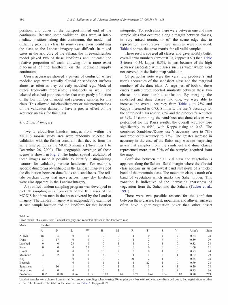
interpreted. For each class there were between one and nine
sample sites that occurred along a margin between classes,
in very mixed terrain, or off the scene edge due to
reprojection inaccuracies; these samples were discarded.
Table 4 shows the error matrix for all valid samples.
These results covered all classes and gave notably better
overall error numbers (error=0.70, kappa=0.69) than Table
3 (error=0.54, kappa=0.53), in part because of the high
accuracy associated with classes such as water which were
not covered in the Raisz map validation.
Of particular note were the very low producer’s and
user’s accuracies of the sandsheet class and the marginal
numbers of the dune class. A large part of both of these
errors resulted from spectral similarity between these two
classes and considerable confusion. By merging the
sandsheet and dune classes into one, we were able to
increase the overall accuracy from Table 4 to 75% and
Kappa increased to 0.75. Similarly, the user’s accuracy for
the combined class rose to 72% and the producer’s accuracy
to 69%. If combining the sandsheet and dune classes was
performed for the Raisz results, the overall accuracy rose
significantly to 65%, with Kappa rising to 0.63. The
combined Sandsheet/Dunes user’s accuracy rose to 78%
and producer’s accuracy to 77%. The greater increase in
accuracy in the case of the Raisz map was not surprising
given that samples from the sandsheet and dune classes
represented more than 50% of the samples acquired from
the map.
Confusion between the alluvial class and vegetation is
apparent along the Sahara–Sahel margin where the alluvial
class appears in an east–west band just north of a thicker
band of the mountain class. The mountain class is north of a
band of vegetation which marks the Sahel proper. This
zonation is indicative of the increasing sparseness of
vegetation from the Sahel into the Sahara (Tucker et al.,
1991).
There were two possible reasons for the confusion
between these classes. First, mountains and alluvial surfaces
often have higher vegetation cover than other desert
m map
R T S V User’s Sum
1 0 4 2 0.64 28
1 2 6 0 0.59 29
1 2 1 0 0.82 28
0 0 0 0 1.00 21
0 0 1 0 0.83 24
1 1 0 1 0.62 29
21 2 1 0 0.75 28
1 22 1 0 0.79 28
3 3 8 1 0.29 28
0 1 0 19 0.73 26
.69 0.72 0.67 0.36 0.83 0.70 269
amples per class with some images discarded due to bad registration or other

J.-A.C. Ballantine et al. / Remote Sensing of Environment 97 (2005) 470–483 481
landforms. Many of the training sites for the alluvial class
came from hamadas where springs and watercourses, and
therefore vegetation, may occur, and plateaus where
seasonal grasslands may be found. Orographic rainfall
effects in mountains, even in the Sahara, allows for some
vegetation cover.
A second reason for confusion is spectral. The existence
of vegetation on alluvial and mountain surfaces effectively
makes this an impure endmember because the reflectance
spectrum of these sites is some combination of a plant or
NPV spectrum and a mineral soil spectrum. In addition,
both plant and mountain spectra are dark, with the
mountain spectra bearing some resemblance to NPV,
especially dry grass (Fig. 3a,c,d). As vegetation thins from
the Sahel into the Sahara, the mountain and alluvial classes
act as transitional classes from vegetation to unvegetated
landforms where a three-endmember class combination
with vegetation does not represent these areas as well. This
results in the east–west banding in Fig. 7 from the Sahel
to the Sahara with the mountain class just north of
vegetation, probably representing dry grasses. North of
the ‘‘mountain’’ band is a band of reg where three-
endmember models between vegetation and reg are
required with the reg class having a greater cover fraction.
As is typical of the Sahel, the red stems endmember is
most frequently paired with reg, but the rabbitbrush and
dry grass endmembers are also common. Finally, the
alluvial class represents the edge of the vegetated zone
south of the arid heart of the desert.
Although these confusions require further investigation
of the three-endmember cases and how the classes overlap,
the accuracy of the landform map produced by the MESMA
is good, considering the spatial resolution of the imagery.
4.8. Maximum likelihood classification
To test the efficacy of the MESMA methodology, we
compared our results to those of a standard supervised
Table 5
Error matrix of classes from Landsat imagery and modeled classes from the max
Model Landsat
A D L W B M
Alluvial 15 1 2 0 4 3
Dune 1 20 3 0 0 0
Lakebed 0 1 16 0 0 0
Water 0 0 0 17 0 0
Basalt 1 0 0 0 13 9
Mountain 0 2 0 1 5 12
Reg 4 6 0 0 0 0
Bedrock 3 1 3 2 1 1
Sandsheet 1 3 0 2 0 1
Vegetation 8 0 0 0 0 0
Producer’s 0.45 0.59 0.67 0.77 0.57 0
Landsat samples were chosen from a stratified random sampling scheme using 30 s
errors. The format of the table is the same as for Table 3. Kappa=0.55.
classification of the MODIS imagery in Fig. 2. We chose a
maximum likelihood classifier so as to be able to express the
statistical distribution of training spectra for each class.
The classifier was trained using the Landsat imagery,
which was deemed to be the highest quality dataset
available. Each of the 20 scenes used for the error analysis
shown in Table 4 was examined for areas that were
interpretable as being indisputably of a given class. These
areas were transferred to the MODIS imagery to create the
training polygons. Each class had from 4 to 18 training
polygons, with the more common classes having more
polygons. The mountain class was the only class with
greater than 10% aerial coverage in Fig. 7 that had fewer
than 10 training sites. The basalt and vegetation classes were
supplemented with training sites from outside of the Landsat
coverage that were still clearly from those classes in the
MODIS imagery (e.g. the Black Haruj basalt flows of Libya
and Sahelian vegetation).
The results of this classification were compared with the
same Landsat validation sites used to create the error matrix,
Table 4. Although the same training set was used for the
error analysis, we feel this was justified because the training
sites and error analysis sites were chosen independently. The
Landsat data represented the best available dataset for both
of these tasks. The error matrix comparing the maximum
likelihood classifier to the Landsat reference is shown in
Table 5.
The maximum likelihood classification’s error results
were significantly worse than those of the MESMA derived
landform map when compared with the Landsat reference
data (overall accuracy of 56% and kappa of 0.55 as
compared with 70% overall accuracy and a kappa of 0.69
for the MESMA derived map). In the case of the maximum
likelihood classification, the alluvial, mountain, reg, and
sandsheet classes were poorly classified with user’s and
producer’s accuracies below 50%.
It is probable that the maximum likelihood classifier did
not perform well in this case because of the broad spectral
imum likelihood classification
R E S V User’s Sum
5 4 2 2 0.39 38
0 0 4 0 0.71 28
0 1 3 0 0.76 21
0 0 0 0 1.00 17
0 0 0 0 0.57 23
3 7 0 0 0.40 30
13 1 4 1 0.45 29
3 17 1 0 0.53 32
5 3 8 1 0.33 24
0 0 0 19 0.70 27
.46 0.45 0.52 0.36 0.83 0.56 269
amples per class with some images discarded due to bad registration or other

J.-A.C. Ballantine et al. / Remote Sensing of Environment 97 (2005) 470–483482
definition of each landform class which produces a high
variance at each wavelength. At this resolution, many of the
landforms truly are mixtures which MESMA was able to
account for. The supervised classification, which tried to
force each pixel’s spectrum to fit a mean spectrum with a
large variance, had a more difficult time with these mixed
pixels. Furthermore, MESMA accounts for the variance that
is added to each class as a result of surface roughness and
shadowing because these are modeled by the shade
endmember. Variability in brightness around the mean can
be a problem for supervised classifiers.
We also performed a minimum distance to the mean
supervised classification using the endmember spectra shown
in Fig. 3a–d. The results of this classification were
considerably worse than both the MESMA-based, and the
maximum likelihood classifications (overall accuracy=47%,
Kappa=0.45).
Given the poor classification performance of the super-
vised classifications, there is a clear accuracy benefit in the
MESMA approach. Furthermore, the MESMA approach
provides additional information about the fractional cover-
age of landforms and vegetation that is not available in other
classification methods.
As a final assessment of the quality of the landform map
product, we compared our accuracy results with those of
Hansen et al. (2000). This was the closest study in
methodology and scale that we could find, but it is worth
noting that they used decision trees to estimate fractional
cover and were studying land cover at the global scale. Our
overall accuracy result of 70% is marginally better than their
overall accuracy of 65%, showing that this range of
accuracy is acceptable for a product at the sub-continental
scale.
5. Conclusions
Moderate resolution satellite imagery is an effective tool
for mapping desert landforms. This paper demonstrates the
use of MESMA at the subcontinental scale where previous
studies using SMA techniques have largely focused on
smaller regions. Endmembers representing pure landforms
were used to model the imagery with the addition of a set of
mostly reference vegetation spectra to provide a separate
vegetation endmember where applicable. A landform map
of Africa north of 10- was produced with 10 landform
classes based on majority endmember fractions.
The landform map improved on the existing Raisz (1952)
landform map by creating a digital product, at moderate
resolution, to which properties could be assigned for
analytical or modeling purposes. Furthermore, the use of
vegetation spectra allowed the creation of a map of
fractional vegetation cover for the Sahara.
The modeled landform map identified dunes and regs as
the dominant landform classes in North Africa at 22% and
21% coverage, respectively. Sandsheets comprised 15% of
the surface area, alluvial fans 14%, mountains 9%, and
etched bedrock 3%. Areas where vegetation was the
majority cover fraction were 13% of the study area, but
because the majority of the vegetation is in the Sahel, this
figure is dependent on the arbitrary southern cutoff of 10- Nlatitude. Minor classes with 1% or less areal coverage were
basalt, lakebeds, and open water.
The total accuracy of the landform classification was
54% when the image classification results were compared to
the Landform Map of North Africa of Raisz (1952), used in
the original image endmember determination. These results
showed some confusion between regs and alluvial surfaces
as well as between sandsheets and dunes. A stratified
random sampling approach using Landsat data for valida-
tion produced a higher accuracy of 70% and eliminated the
confusion between the alluvial and reg classes. However,
there was considerable spectral confusion between dunes
and sandsheets. Combining these classes increased overall
accuracy to 73% for the Raisz map and 75% for the Landsat
validation. The gradation of vegetation from the Sahel
northward into the Sahara also posed classification problems
with mountain and alluvial classes mimicking dark, semi-
vegetated surfaces.
When compared with a maximum likelihood supervised
classification, the MESMA approach improved the classi-
fication accuracy considerably from 56% to 70%. The
maximum likelihood classifier had particular difficulty
classifying the alluvial, mountain, reg, and sandsheet
classes.
In this paper, we established an accurate sub-continental
scale landform classification. These landforms could be
used as the basis for an erodibility map for continental-
scale wind erosion studies, or for other purposes where
geomorphic properties are significant. The creation of a
spectrally based map of the permanent background land-
forms of the Sahara also allows for the use of a partial
unmixing (Boardman et al., 1995) of vegetation to monitor
changing vegetation cover over time. In this way seasonal
and interannual variations in vegetation vigor could be
assessed where vegetation is present in the marginal lands
at the fringes of the Sahara. Furthermore, the MODIS
imagery is at a fine enough resolution that changes in land
use could be assessed with these methods, thereby
providing another tool for trying to understand the
influence of human activities and how the natural environ-
ment might respond to those activities based on the
underlying landforms. The methodology presented here is
also transportable to other arid and semi-arid parts of the
world where an understanding of landforms would be
desirable.
Acknowledgements
The authors gratefully acknowledge the financial support
of NASA through an Inter-disciplinary Science Grant

J.-A.C. Ballantine et al. / Remote Sensing of Environment 97 (2005) 470–483 483
(NAG5-9671) and an Earth System Science 33 Graduate
Fellowship (NGT5-30332). We also thank Thomas Dunne,
Natalie Mahowald, and Oliver Chadwick for their helpful
comments.
References
Boardman, J. W., Kruse, F. A., & Green, R. O. (1995). Mapping target
signatures via partial unmixing of AVIRIS data in summaries of the 5th
JPL airborne earth science workshop. JPL Publication 95-1, 1, 23–26.
Bovill, E. W. (1968). The golden trade of the moors. Oxford, U.K.’ OxfordUniversity Press.
Clements, T., et al. (1957). A study of desert surface conditions.
Headquarters Quartermaster General Research and Development Com-
mand, Environmental Protection Research Division
Congalton, R. G. (1991). A review of assessing the accuracy of
classifications of remotely sensed data. Remote Sensing of Environment,
37, 35–46.
Defries, R. S., Hansen, M. C., & Townshend, J. R. G. (2000). Global
continuous fields of vegetation characteristics: A linear mixture model
applied to multi-year 8 km AVHRR data. International Journal of
Remote Sensing, 21, 1389–1414.
Dennison, P. E., & Roberts, D. A. (2003). Endmember selection for
multiple endmember spectral mixture analysis using endmember
average RMSE. Remote Sensing of Environment, 87, 123–135.
Elmore, A. J., Mustard, J. F., Manning, S. J., & Lobell, D. B. (2000).
Quantifying vegetation change in semiarid environments: Precision and
accuracy of spectral mixture analysis and the normalized difference
vegetation index. Remote Sensing of Environment, 73, 87–102.
Friedl, M. A., McIver, D. K., Hodges, J. C. F., Zhang, X. Y., Muchoney, D.,
& Strahler, A. H., et al. (2002). Global land cover mapping from
MODIS: Algorithms and early results. Remote Sensing of Environment,
83, 287–302.
Funk, C. C., Theiler, J., Roberts, D. A., & Borel, C. C. (2001). Clustering to
improve matched filter detection of weak gas plumes in hyperspectral
thermal imagery. IEEE Transactions on Geoscience and Remote
Sensing, 39, 1410–1420.
Gillette, D. A. (1999). A qualitative geophysical explanation for ‘‘hot spot’’
dust emission source regions. Contributions to Atmospheric Physics,
72, 67–77.
Goudie, A. S., & Middleton, N. J. (2001). Saharan dust storms: Nature and
consequences. Earth-Science Reviews, 56, 179–204.
Hansen, M. C., Defries, R. S., Townshend, J. R. G., & Sohl berg, R. (2000).
Global land cover classification at 1 km spatial resolution using a
classification tree approach. International Journal of Remote Sensing,
21, 1331–1364.
Kocurek, G., & Lancaster, N. (1999). Aeolian system sediment state:
Theory and mojave desert kelso dune field example. Sedimentology, 46,
505–515.
Luo, C., Mahowald, N. M., & del Corral, J. (2003). Sensitivity study
of meteorological parameters on mineral aerosol mobilization,
transport, and distribution. Journal of Geophysical Research, 108
(D15), 4447.
Mahowald, N. M., Zender, C., Luo, C., Savoie, D., Torres, O., & del Corral,
J. (2002). Understanding the 30-year Barbados desert dust record.
Journal of Geophysical Research, 107(D21), 4561.
Marticorena, B., Bergametti, G., & Legrand, M. (1999). Comparison of
emission models used for large scale simulation of the mineral dust
cycle. Contributions in Atmospheric Physics, 72, 151–160.
McFadden, L. D., Wells, S. G., & Jercinovich, M. J. (1987). Influences of
eolian and pedogenic processes on the origin and evolution of desert
pavements. Geology, 15, 504–508.
Myneni, R. B., Hoffman, S., Knyazikhin, Y., Privette, J. L., Glassy, J., &
Tian, Y., et al. (2002). Global products of vegetation leaf area and
fraction absorbed PAR from year one of MODIS data. Remote Sensing
of Environment, 83, 214–231.
Okin, G. S., & Painter, T. (2004). Effect of grain size on remotely sensed
spectral reflectance of sandy desert surfaces. Remote Sensing of
Environment, 89, 272–280.
Prospero, J. M., Ginoux, P., Torres, O., & Nicholson, S. E. (2002).
Environmental characterization of global sources of atmospheric soil
dust derived from the NIMBUS-7 TOMS absorbing aerosol product.
Reviews of Geophysics, 40.
Raisz, E. (1952). Landform Map of North Africa. Environmental Protection
Branch, Office of the Quartermaster General.
Roberts, D. A., Smith, M. O., & Adams, J. B. (1993). Green vegetation,
nonphotosynthetic vegetation, and soils in AVIRIS data. Remote
Sensing of Environment, 44, 255–269.
Roberts, D. A., Gardner, M., Church, R., Ustin, S., Scheer, G., & Green, R.
O. (1998). Mapping chaparral in the Santa Monica mountains using
multiple endmember spectral mixture models. Remote Sensing of
Environment, 65, 267–279.
Roberts, D. A., Dennison, P. E., Gardner, M. E., Hetzel, Y., Ustin, S. L., &
Lee, C. T. (2003). Evaluation of the potential of Hyperion for fire
danger assessment by comparison to the airborne visible/infrared
imaging spectrometer. IEEE Transactions on Geoscience and Remote
Sensing, 41, 1297–1310.
Smith, M. O., Ustin, S. L., Adams, J. B., & Gillespie, A. R. (1990).
Vegetation in deserts I. A regional measure of abundance from
multispectral images. Remote Sensing of Environment, 48, 70–76.
Taylor, R. G., & Howard, K. W. F. (1999). Lithological evidence for the
evolution of weathered mantles in Uganda by tectonically controlled
cycles of deep weathering and stripping. Catena, 35, 65–94.
Theseira, M. A., Thomas, G., & Sannier, C. A. D. (2002). An evaluation of
spectral mixture modelling applied to a semi-arid environment. Interna-
tional Journal of Remote Sensing, 23, 687–700.
Thomas, D. S. G. (1997). Sand seas and aeolian bedforms in arid zone
geomorphology. In D. S. G. Thomas (Ed.), Process form and change in
drylands (2nd edition). New York’ John Wiley and Sons, Ltd.
Tompkins, S., Mustard, J. F., Pieters, C. M., & Forsyth, D. W. (1997).
Optimization of endmembers for spectral mixture analysis. Remote
Sensing of Environment, 59, 472–489.
Tsvetsinskaya, E. A., Schaaf, C. B., Gao, F., Strahler, A. H., Dickinson, R.
E., Zeng, X., et al. (2002). Relating MODIS-derived surface albedo to
soils and rock types over Northern Africa and the Arabian peninsula.
Geophysical Research Letters, 29, 1–4.
Tucker, C. J., Dregne, H. E., & Newcomb, W. W. (1991). Expansion
and contraction of the Sahara Desert from 1980 to 1990. Science, 253,
299–301.
Tucker, C. J., & Nicholson, S. E. (1999). Variations in the size of the Sahara
Desert from 1980 to 1997. Ambio, 28, 587–591.
Weiss, J. L., Gutzler, D. S., Allred Coonrod, J. E., & Dahm, C. N. (2004).
Long-term vegetation monitoring with NDVI in a diverse semi-arid
setting, central New Mexico, USA. Journal of Arid Environments, 58,
249–272.