mapping greater sage-grouse preliminary priority habitat...
TRANSCRIPT
Mapping Greater Sage-Grouse Preliminary Priority Habitat in the
Bi-State DPS
Technical Advisory Committee

Purpose Develop a scientifically defensible decision support tool (models and maps) for management of sage-grouse populations FOCUS MANAGEMENT EFFORTS ON THE AREAS MOST MEANINGFUL FOR SAGE-GROUSE POPULATIONS

Hierarchical Approach
Decision support tool to map areas
important to sage-grouse populations
Microhabitat objectives – factors that influence sage-grouse
populations

Hierarchical Approach
Decision support tool to map areas
important to sage-grouse populations
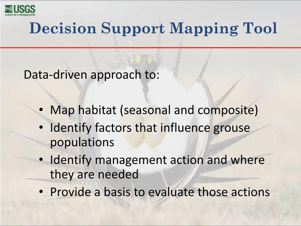
Data-driven approach to:
• Map habitat (seasonal and composite)
• Identify factors that influence grouse populations
• Identify management action and where they are needed
• Provide a basis to evaluate those actions
Decision Support Mapping Tool
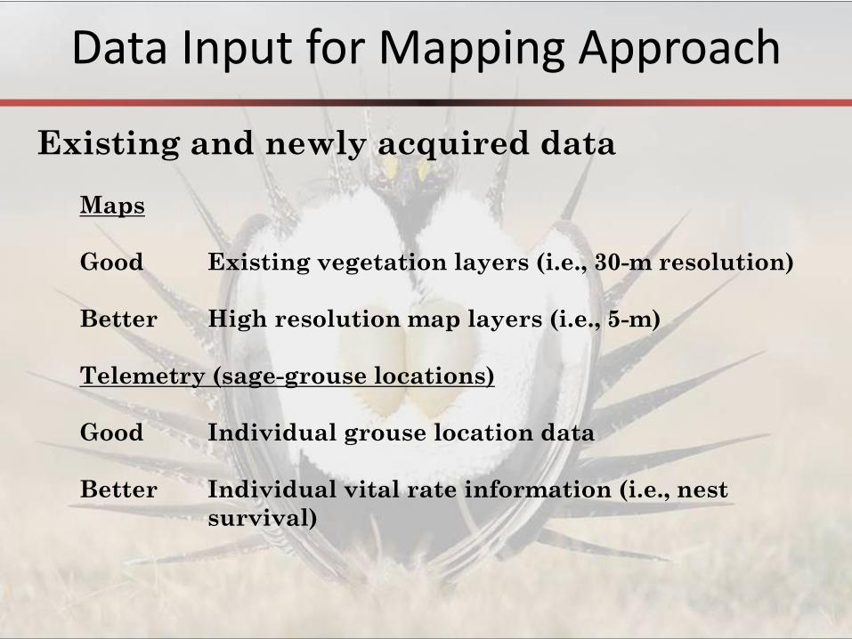
Existing and newly acquired data
Maps
Good Existing vegetation layers (i.e., 30-m resolution)
Better High resolution map layers (i.e., 5-m)
Telemetry (sage-grouse locations)
Good Individual grouse location data
Better Individual vital rate information (i.e., nest
survival)
Data Input for Mapping Approach

Bi-State Distinct Population Segment
Bi-State DPS

Composite Land Cover Map of Bi-State DPS
15 Model Variables at 2 spatial scales Pinyon-juniper phases Three sagebrush communities Upland and lowland non-sagebrush shrubland communities Annual and Perennial Grasslands Agricultural areas Two topographic variables Roads Urbanization Index
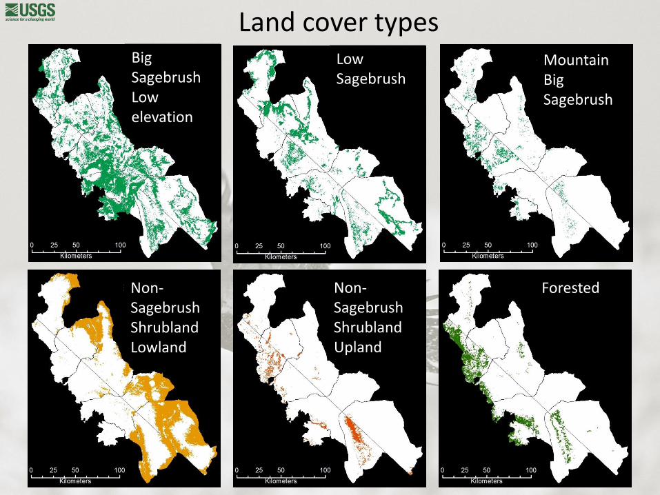
Land cover types Big Sagebrush Low elevation
Low Sagebrush
Mountain Big Sagebrush
Non-Sagebrush Shrubland Lowland
Non-Sagebrush Shrubland Upland
Forested
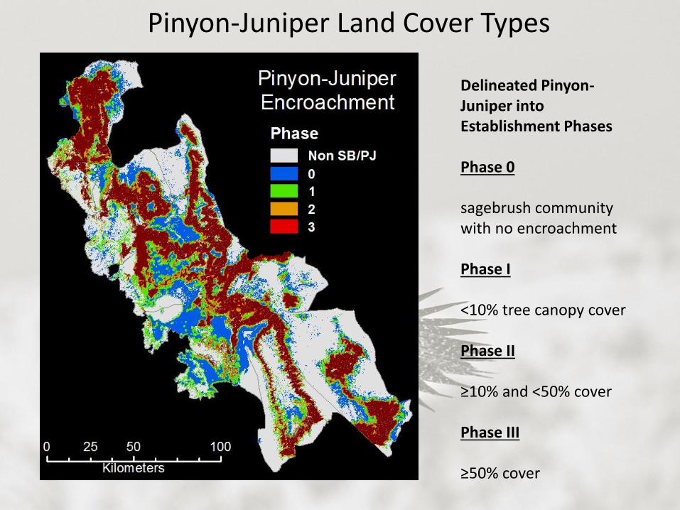
Pinyon-Juniper Land Cover Types
Delineated Pinyon-Juniper into Establishment Phases Phase 0 sagebrush community with no encroachment Phase I <10% tree canopy cover Phase II ≥10% and <50% cover Phase III ≥50% cover
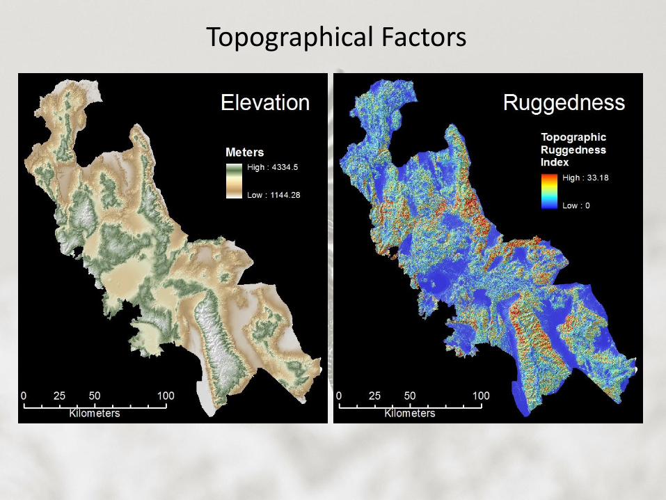
Topographical Factors

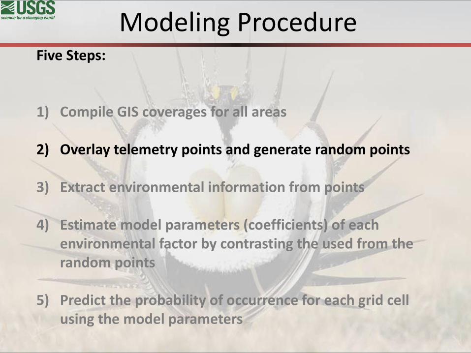
Five Steps:
1) Compile GIS coverages for all areas
2) Overlay telemetry points and generate random points
3) Extract environmental information from points
4) Estimate model parameters (coefficients) of each
environmental factor by contrasting the used from the random points
5) Predict the probability of occurrence for each grid cell using the model parameters
Modeling Procedure
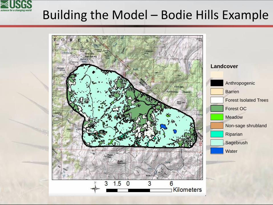
Building the Model – Bodie Hills Example
Legend
VegVectorclipped
<all other values>
Landcover
Anthropogenic
Barren
Forest Isolated Trees
Forest OC
Meadow
Non-sage shrubland
Riparian
Sagebrush
Water
Five Steps:
1) Compile GIS coverages for all areas
2) Overlay telemetry points and generate random points
3) Extract environmental information from points
4) Estimate model parameters (coefficients) of each
environmental factor by contrasting the used from the random points
5) Predict the probability of occurrence for each grid cell using the model parameters
Modeling Procedure

Overlay Grouse Telemetry Locations

Generate Random Points

Five Steps:
1) Compile GIS coverages for all areas
2) Overlay telemetry points and generate random points
3) Extract environmental information from points
4) Estimate model parameters (coefficients) of each
environmental factor by contrasting the used from the random points
5) Predict the probability of occurrence for each grid cell using the model parameters
Modeling Procedure
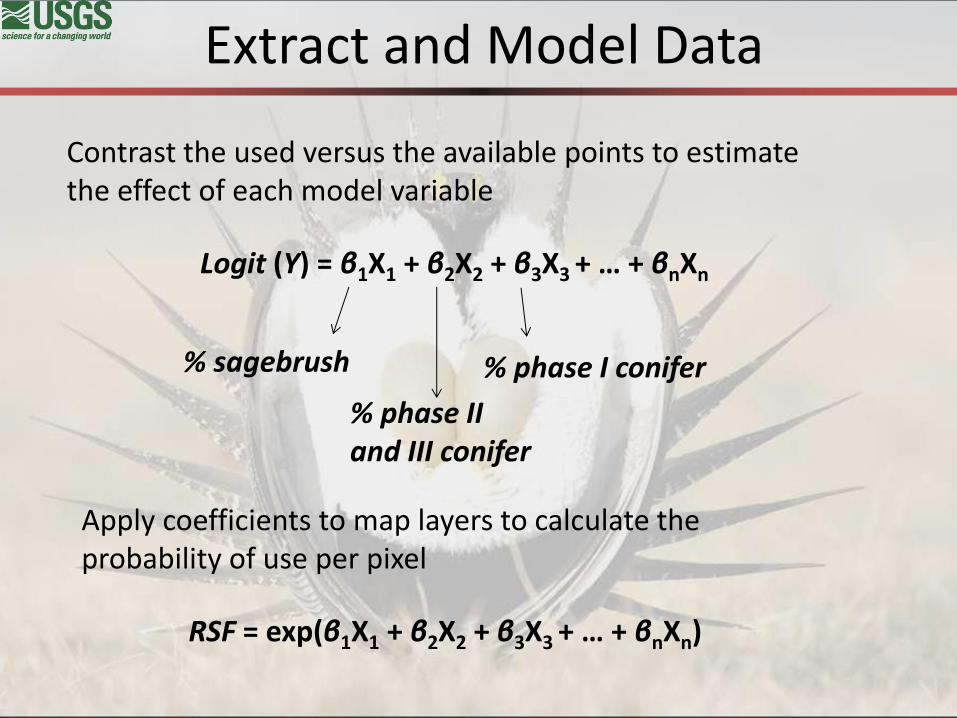
Contrast the used versus the available points to estimate the effect of each model variable
Logit (Y) = β1X1 + β2X2 + β3X3 + … + βnXn
% sagebrush
% phase II and III conifer
% phase I conifer
RSF = exp(β1X1 + β2X2 + β3X3 + … + βnXn)
Apply coefficients to map layers to calculate the probability of use per pixel
Extract and Model Data

Five Steps:
1) Compile GIS coverages for all areas
2) Overlay telemetry points and generate random points
3) Extract environmental information from points
4) Estimate model parameters (coefficients) of each
environmental factor by contrasting the used from the random points
5) Predict the probability of occurrence for each grid cell using the model parameters
Modeling Procedure
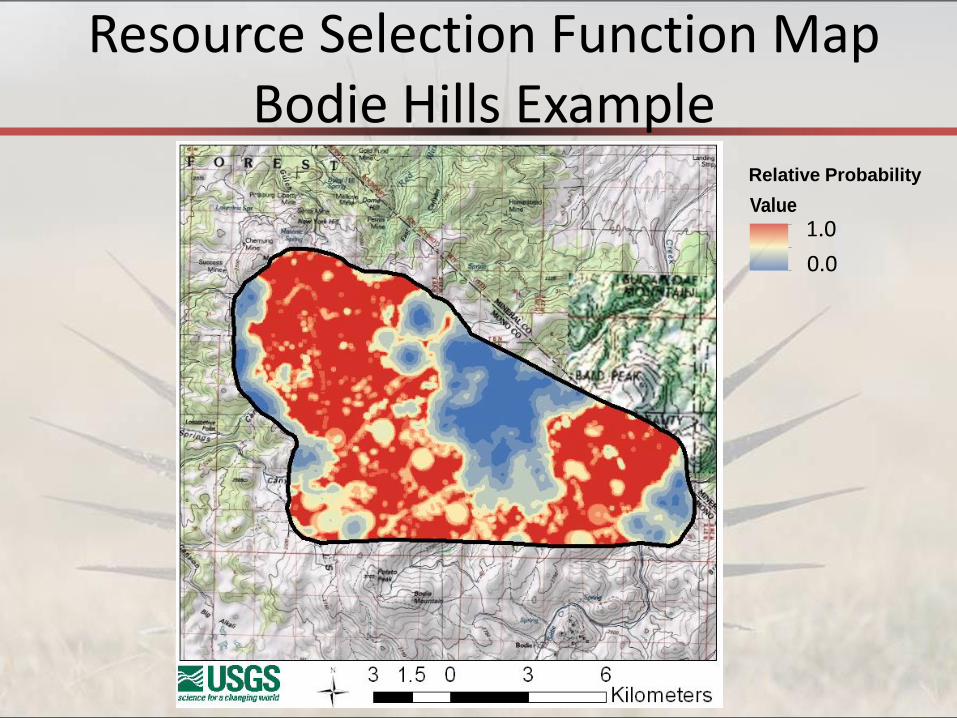
Resource Selection Function Map Bodie Hills Example
Legend
bistatersf2prb
ValueHigh : 0.550473
Low : 0.323284
1.0
0.0
Relative Probability
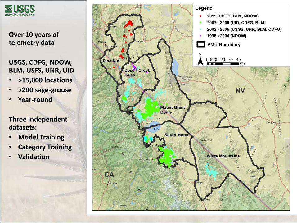
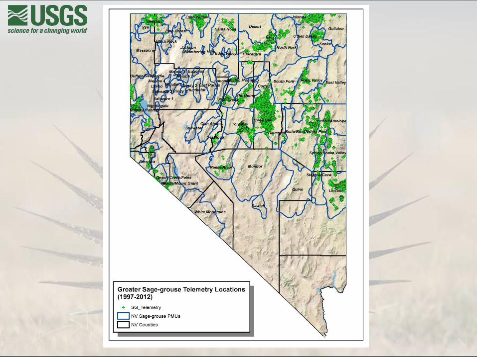
Over 10 years of telemetry data
USGS, CDFG, NDOW, BLM, USFS, UNR, UID
• >15,000 locations
• >200 sage-grouse
• Year-round
Three independent datasets:
• Model Training
• Category Training
• Validation
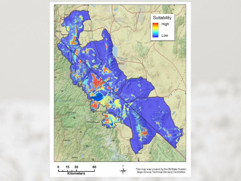

TAC Habitat Model NDOW Habitat Categorization
Comparison between Maps
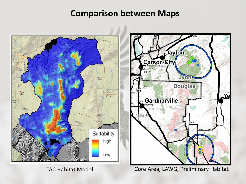
TAC Habitat Model Core Area, LAWG, Preliminary Habitat
Comparison between Maps
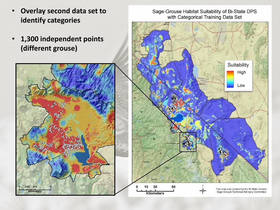
• Overlay second data set to identify categories
• 1,300 independent points (different grouse)

EXAMPLE Leks (traditional breeding grounds) on the near the edge of priority habitat Potential effects of nearby disturbance
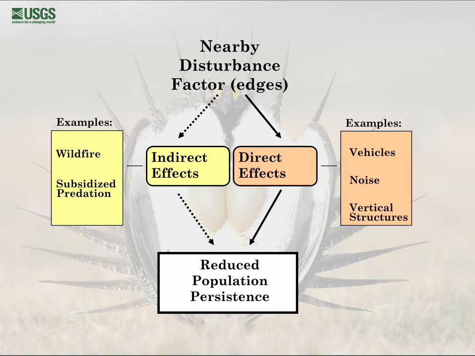
Direct
Effects
Indirect
Effects
Reduced
Population
Persistence
Vertical Structures
Vehicles
Noise Subsidized Predation
Wildfire
Examples: Examples:
Nearby
Disturbance
Factor (edges)

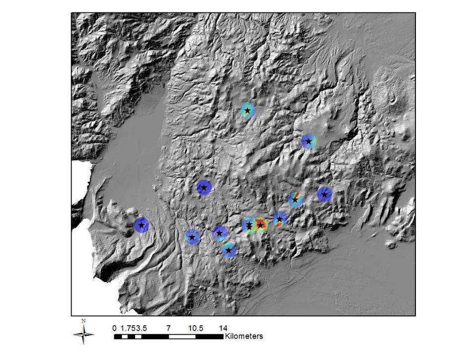
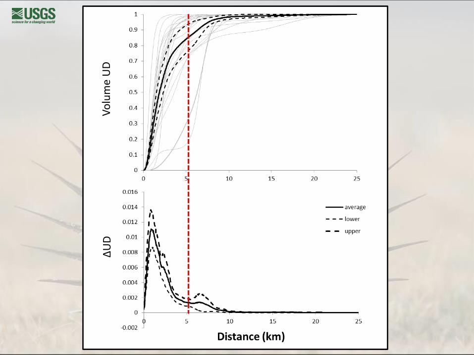
Edge Effects - Utilization Distribution Analysis
1) Calculated seasonal use areas (utilization distribution; UD) for each grouse by season
2) Calculated volume of UD within each 30-m increase distance from lek
3) Diminishing returns in UD analysis with increasing buffer distance


Vo
lum
e U
D
∆U
D
Vo
lum
e U
D
∆U
D

Diminishing Returns
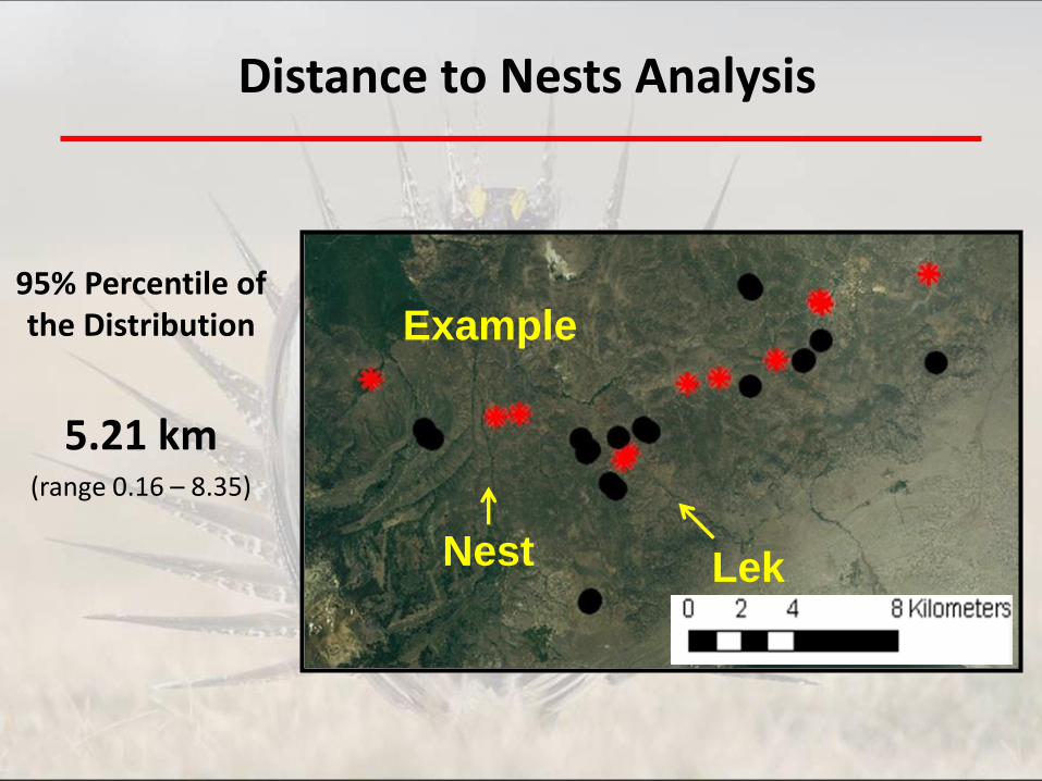
Lek Nest
Distance to Nests Analysis
Example
95% Percentile of the Distribution
5.21 km (range 0.16 – 8.35)
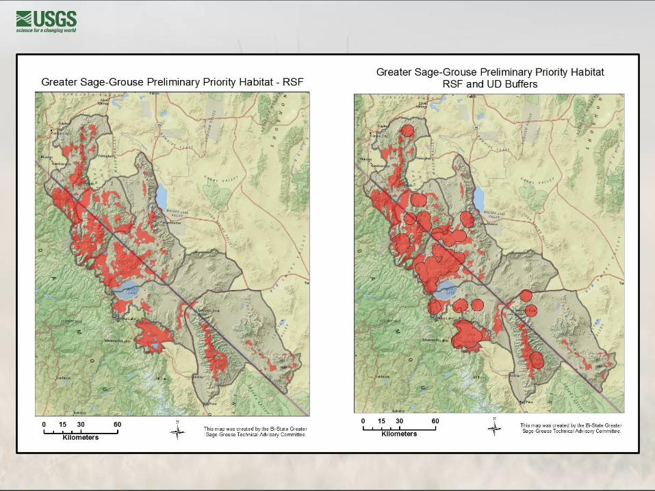

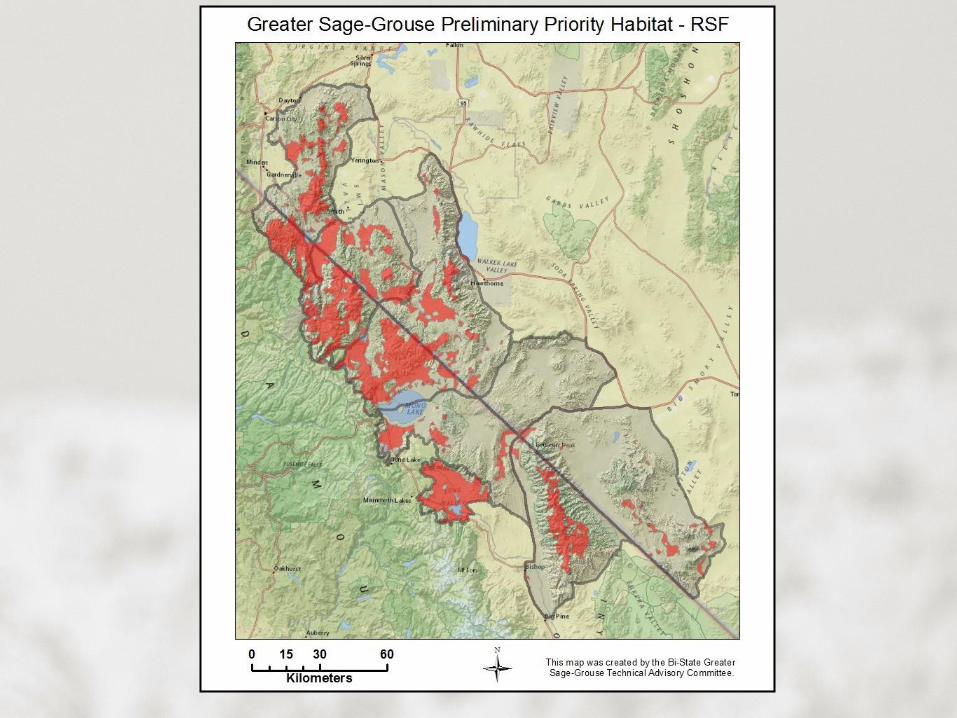
Area with buffers 1,371,760 acres (30%) Areas without buffers 1,047,020 acres (23%)
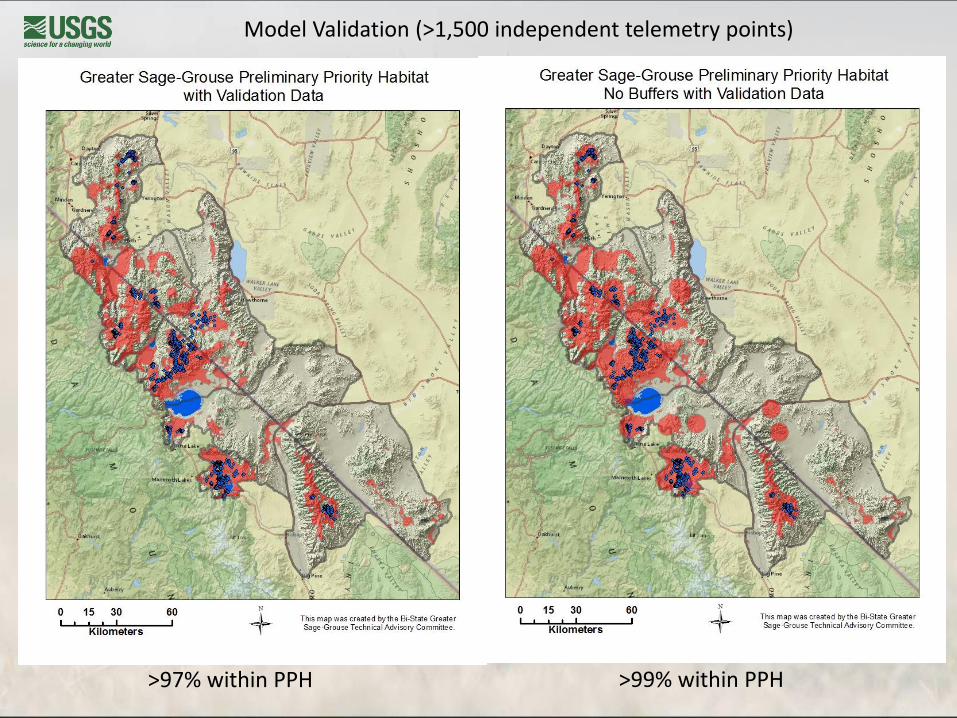
Model Validation (>1,500 independent telemetry points)
>97% within PPH >99% within PPH

GPS Technology

EARTH GRAPHIC

Acknowledgments Nevada Department Of Wildlife
California Department of Fish and Game University of Nevada Reno
Idaho State University University of Idaho
Bureau of Land Management (CA) Bureau of Land Management (NV)
US Fish and Wildlife Service USDA Forest Service
