HABITAT RESOURCE SELECTION BY GREATER SAGE GROUSE WITHIN OIL

AND GAS DEVELOPMENT AREAS IN NORTH DAKOTA AND MONTANA

BY

KRISTIN A. FRITZ

A thesis submitted in partial fulfillment of the requirements for the

Master of Science

Major in Wildlife and Fisheries Sciences

South Dakota State University

2011

iii

Acknowledgments

This research would not have been possible without the funding. Funding for this

project was provided by U.S. Forest Service, Rocky Mountain Research Station, North

Dakota Game and Fish Department, Bureau of Land Management, and through matching

funds from South Dakota State University.

I can’t thank my major advisor K.C. Jensen enough for this absolutely fantastic

opportunity to gain knowledge and broaden my outlook on life. You have one of the

biggest hearts of anyone I have ever met and I’m so glad you gave me the opportunity to

work under you on this project. I am indebted to Dr. Robert W. Klaver for his constant

support and assistance with statistical analysis and for serving on my graduate committee.

I would also like to thank Dr. Kenneth F. Higgins for taking time out of his schedule to

review this manuscript, serve on my graduate committee, and provide suggestions. I must

also include the Wildlife and Fisheries Department secretaries Carol Jacobson, Terri

Symens, and Diane Drake. Their tireless work in taking care of all my office paperwork

and the countless emails helping me track down whatever and whomever that I needed

during this study was greatly appreciated.

I need to give thanks to my wonderful technician (Rebecca Rosenbaum) that was

willing to go above and beyond. We put in incredibly long days and nights, if it wasn’t

for the can-do attitude this project would not have gotten off the ground! Thanks for all

the understanding and wiliness to sick the long field season out! In addition, sincere

thank you is extended to all fellow graduate students that were there for me when I need a

shoulder to lean on and a brain to bounce ideas off of!

iv

This project would not have been possible without the cooperation of several

landowners within my study area. I need to send a special sincere thank you to Don and

Pam Hestiken for being my home away from home; not only did you let me use your

running water for taking showers and washing clothes but you were there to help wrangle

snakes out of my kitchen and help with four-wheeler issues with just a phone call! I will

be forever indebted to both of you for all you did for me! Also huge thank you to Kelly

and Susie Stearns for making me feel like family and inviting me to all the events in the

area, I just can’t thank you enough.

To my Fish and Wildlife Service family - These people I need to thank from the

bottom of my heart. I consider them more than just friends I consider them part of my

family. Their conditional support and words of wisdom were the glue that held me

together on the days that I needed it the most. A heartfelt thank you to Maggie Anderson,

Gregg Knutsen, Ashley Hitt, and Maria Fosado for all going above and beyond when I

needed it the most!

Most importantly, I extend my love and gratitude to my family for their never-

ending support and understanding these past two years. Without their love and never

ending support I don’t know where I would be today, they were truly my foundation.

This experience has made me realize how incredible they are and how much I cherish

every moment that I get to spend with them. I am truly blessed to be a part of an amazing

strong family. Thank to everyone who made this chapter of my life enjoyable and

achievable. I will never be able to thank you all enough!!

v

Abstract

HABITAT RESOURCE SELECTION BY GREATER SAGE GROUSE WITHIN OIL

AND GAS DEVELOPMENT AREAS IN NORTH DAKOTA AND MONTANA

Kristin A. Fritz

July 2011

Populations of greater sage-grouse (Centrocercus urophasianus; hereafter sage

grouse) have declined substantially throughout a majority of their range (Connelly and

Braun 1997, Schroeder et al. 1999, 2004). There has also been a corresponding decline

in sage (Artemisia spp.) habitat quantity and quality. Consequently, sage grouse

populations have declined in response to a pattern of land-use changes that have reduced

and degraded sagebrush ecosystems (Hemstrom et al. 2002). Sage grouse are native to

the sagebrush steppe ecosystem, and their distribution closely follows that of sagebrush.

Important mineral resources (i.e., gas, oil) are coincident with sage grouse habitats across

much of the western United States. Sagebrush steppe habitats along the Cedar Creek

Anticline of southeastern Montana and southwestern North Dakota exemplify important

sage grouse habitats that overlay mineral resources which are currently being extracted,

or have been targeted for development. There are many concerns involving the responses

of sage grouse and their use of habitats that have been, or potentially will be impacted by

mineral development and associated infrastructure (i.e., roads, power lines, buildings,

generators, water outflows). The primary objectives of this study were to: (1) determine

the habitat suitability within the oil and gas developed regions of Bowman County, North

vi

Dakota and Fallon County, Montana and (2) determine what factors may cause

avoidance.

Vegetation measurements were taken at 67 nest sites and 166 random sites

between 2005 and 2009 and analyzed using an Information Theoretic approach with

logistic regression. The top model that predicted sage grouse use included total percent

vegetation cover, the visual obstruction at the nest bowl, the visual obstruction at one

meter away from the nest bowl, 0-m VOR, 1-m VOR grass height, and year affect (AICc

weight = 0.54). When I compared the area of intense use to areas of relative non-use, I

found that there were four competing models; the top model included total percent

vegetation cover and grass height (AICc weight = 0.25). When I compared density of

roads I found that the area of avoidance contained 120.9 km (0.0317 km/ha) of roads

whereas the area of use had 44 km (0.014 km/ha) of roads. Hence, the density of roads

within the area of avoidance was about 2.6 times greater than the density within the area

of use.

vii

Table of Contents

Acknowledgments.............................................................................................................. iii

Abstract ............................................................................................................................... v

Table of Contents .............................................................................................................. vii

List of Tables ................................................................................................................... viii

List of Figures .................................................................................................................... ix

Introduction ......................................................................................................................... 1

Study Area .......................................................................................................................... 7

Methods............................................................................................................................... 9

Results ............................................................................................................................... 15

Discussion ......................................................................................................................... 19

Management Implications and Future Resource Needs.................................................... 23

Literature Cited. ................................................................................................................ 38

viii

List of Tables

Table Page

1. Results from logistic regression models predicting greater sage grouse nest

sites (n=67) versus random sites (n=166) in southwestern North Dakota

and northeastern Montana, USA, 2005, 2006, 2007, and 2009 .............................25

2. Mean vegetation characteristics of nest sites and random sites over years

2005, 2006, 2007, and 2009 for greater sage grouse used in logistic

regression models in southwestern North Dakota and northeastern

Montana, USA. ......................................................................................................26

3. Mean vegetation characteristics of random points inside area of use and

random sites in area of avoidance over years 2005, 2006, 2007, and 2009 for

greater sage grouse used in logistic regression models in southwestern North

Dakota and northeastern Montana, USA. ..............................................................27

4. Results from logistic regression models predicting greater sage grouse

area of use (n=69) versus area of avoidance (n=41) in southwestern

North Dakota and northeastern Montana, USA, 2005, 2006, 2007, and 2009 .....28

5. Results from logistic regression models predicting greater sage grouse

nest sites with road density in km as a variable (n=67) versus random sites

(n=166) in southwestern North Dakota and northeastern Montana,

USA, 2005, 2006, 2007, and 2009 .........................................................................29

6. Results from logistic regression models predicting greater sage grouse

nest sites with road density in km as a variable (n=41) versus random sites

(n=69) in southwestern North Dakota and northeastern Montana,

USA, 2005, 2006, 2007, and 2009 .........................................................................30

ix

List of Figures

Figure Page

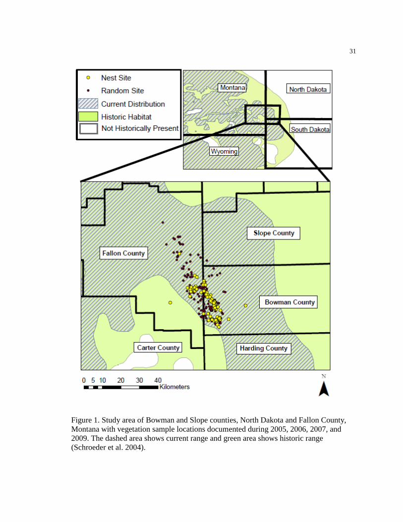
1. Study area of Bowman and Slope counties, North Dakota and Fallon County,

Montana with vegetation sample locations documented during 2005, 2006,

2007, and 2009. The dashed area shows current range and green area shows

historic range (Schroeder et al. 2004) ....................................................................31

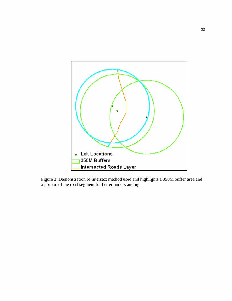
2. Demonstration of intersect method used and highlights a 350M buffer area

and a portion of the road segment for better understanding ..................................32

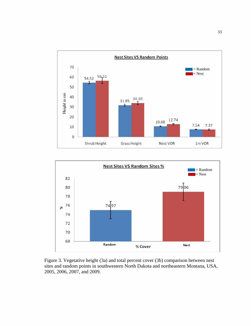
3. Vegetation comparison between nest sites and random points in

southwestern North Dakota and northeastern Montana, USA, 2005, 2006,

2007, and 2009 .......................................................................................................33

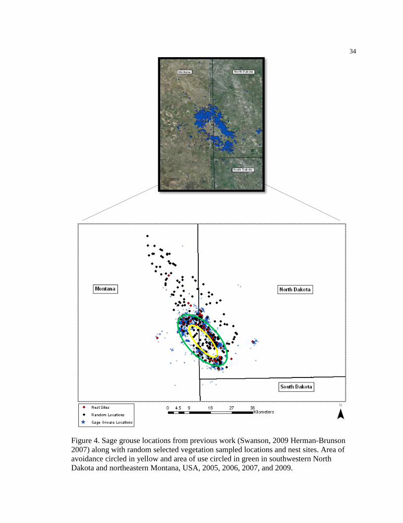
4. Sage grouse locations from previous work (Swanson, 2009

Herman-Brunson, 2007) along with random selected vegetation sampled

locations and nest sites. Area of avoidance circled in yellow and area of use

circled in green in southwestern North Dakota and northeastern Montana,

USA, 2005, 2006, 2007, and 2009 .........................................................................34

5. Vegetation comparison between random locations within area of use

compared to random locations that fall within area of avoidance in

southwestern North Dakota and northeastern Montana, USA, 2005,

2006, 2007, and 2009 .............................................................................................35

6. High density road areas (area of avoidance-top) from areas with lower road

densities (area of use-bottom) within the study area in southwestern

North Dakota and northeastern Montana, USA, 2005, 2006, 2007, and 2009 ......36

7. Distance interpolation for road density in southwestern North Dakota and

northeastern Montana, USA, 2005, 2006, 2007, and 2009 ....................................37

1

Introduction

The historical range of greater sage-grouse (Centrocercus urophasianus; hereafter

sage grouse) has been dramatically reduced since European settlement (Connelly and

Braun 1997, Schroeder et al. 2004). The range of sage grouse has been reduced by 45%

across North America (Schroeder et al. 2004) with an estimated range-wide population

decline of 45-80% and local declines of 17-92% (Connelly et al. 2004). Historically,

sage grouse were found throughout the western U.S. where sagebrush and associated

plant communities existed (Patterson 1952). In addition, Schroeder et al. (2004)

determined that the distribution of sage grouse is clearly associated with the distribution

of sagebrush (Artemisia spp.). Thus, sage grouse are sagebrush obligates because of their

year-round dependence on sagebrush communities (Paige and Ritter 1999).

Sagebrush is required for food, shelter, and as a water source for sage grouse

(Swenson 1987, Fischer et al. 1996, Schroeder et al. 1999). During the winter months,

sagebrush is the only source of food (Hupp and Braun 1989, Welch et al. 1991) with the

sage grouse’s diet consisting of leaves and buds (Welch et al. 1991, Homer et al. 1993,

Connelly et al. 2000). Sagebrush microhabitat is also important during the reproductive

season of the sage grouse; sagebrush coexists with understory forbs that are important for

female sage grouse during nesting and brood-rearing (Drut et al. 1994, Crawford 1997,

Connelly et al. 2000). Sage grouse nest beneath sagebrush (Patterson 1952, Gill 1966,

Connelly et al. 1991, Musil et al. 1994, Sveum et al. 1998), where females may show

nest-site fidelity from year to year (Fischer et al. 1993). Klebenow (1969) and Wallestad

(1975) found that sagebrush provided female sage grouse with nesting cover and early

2

brood-rearing habitat. In the core of the sage grouse range, females typically chose nest

sites with horizontal cover of greater than 73% (Musil et al. 1994, Connelly et al. 2000),

tall residual grasses of greater than 18 cm, and medium shrubs from 40-80 cm of height

(Gregg et al. 1994, Sveum et al. 1998, Connelly et al. 2000). Recent research on the

eastern and northern edges of the range of sage grouse found that sage grouse utilized

taller grass cover as a substitute for the lack of height in sagebrush (Aldredge et al. 2008,

Kaczor et al. 2011).

The decline of sage grouse populations is intimately linked to widespread

sagebrush habitat degradation. The direct and indirect causes of this habitat degradation

are associated with altered fire regimes (Wrobleski and Kauffman 2003), grazing and

agriculture, urbanization, and the development of oil and gas extraction (Connelly et al.

2004). Of the causes, both direct and indirect, oil and gas development is one the most

recent yet the least understood impacts on sage grouse and their habitat. With the

discovery of oil and gas throughout the western U.S. beginning in the 1930s and 1940s,

wildlife habitats have been directly impacted (Braun 1987). Because the production of oil

and gas is predicted to continue for another 20-100 years (Connelly et al. 2004), it is

important to understand the impacts of such development. Increasing energy demands of

an expanding human population pose varied conservation challenges related to North

American wildlife populations (Sawyer et al. 2006, Walker et al. 2007). Once these gas

and oil impacts are better understood, it may be possible to plan future resource

development in ways that minimize impacts to sage grouse populations.

3

There are several factors related to oil and gas development that could negatively

affect sage grouse populations. Oil and gas developments require a certain level of

infrastructure, including construction and usage of roads, erection of well pads, drilling

and extraction of natural resources, establishment of both permanent and non-permanent

facilities and structures, all of which contributes to sagebrush habitat fragmentation.

Consequently, substantial sage grouse population declines have occurred throughout their

range (Connelly and Braun 1997). Braun (1987) suggested that the decline in

Colorado’s sage grouse population is related to the loss of habitat caused by site

preparation, road development, noise from pumping stations, power line development,

and associated human activities. Energy development is known to impact wildlife

directly by altering habitat use (Doherty et al. 2008) and population dynamics (Sorensen

et al. 2008), and indirectly by facilitating the spread of invasive plants (Bergquist et al.

2007) and exotic diseases (Zou et al. 2006, Doherty 2007).

The construction of roads results in direct removal of substantial contiguous

habitat. Roads related to oil and gas development have been associated with reduced

nesting success and increased disturbance during the lekking and brood-rearing periods

(Braun 1998, Braun et al. 2002, Holloran 2005). In Wyoming, nesting success increased

as distance to nearest road increased (Lyon and Anderson 2003, Holloran 2005).

Likewise, when considering habitat fragmentation the construction of a typical well pad

requires 0.8-1.9 hectares and compressor stations along pipelines require 5-7 hectares

(Connelly et al. 2004, Holloran 2005). The long-term effects of pumping stations, and

other permanent facilities are unknown. Direct impacts of oil and gas development on

4

factors such as nesting and lek sites are largely unknown. The placement of these

physical structures has varying impacts on wildlife, and opportunities may exist to

minimize their effects on wildlife. For example, if structures can be placed close

together, rather than farther apart, fewer roads and other related structures may be

necessary. Other effects include soil disturbance along roads and near wells, the spread

of exotic plants species (e.g. cheatgrass (Bromus tectorum) and Canada thistle (Crisium

arvense)) and structures that provide nest and perch sites for raptors (Connelly et al.

2004). Several studies have reported raptors hunting various prey, including sage grouse,

from overhead utility towers and other manmade elevated perches (Wakeley 1978; Graul

1980; Ellis 1984, 1987; Plumpton and Andersen 1997).

Oil and gas development will continue to be to significant threat to sage grouse

because of improved extraction technology and a continued high demand for resources

(Connelly et al. 2004). The U.S. government has already leased more than 7 million

hectares of the federal mineral estate, and the number of producing wells has tripled from

11,000 in the 1980’s to more than 33,000 in 2007 (Naugle et al. 2011). The impacts of

all factors related to oil and gas development need to be understood so that accurate

management recommendations can be made. Although data from Colorado (Braun 1987)

suggest that gas/oil development can cause a decline in sage grouse populations, the

actual reasons for these declines are unknown. As with most wildlife, profound and

permanent changes created within important habitats as a result of altering land use and

ecological patterns can effect the perpetuation of sage grouse (Patterson 1952). Because

of the lack of information concerning the potential impacts of natural gas and oil

5

development within the area, an investigation was prompted concerning the potential

impacts of natural gas and oil development on sage grouse populations within the Cedar

Creek Anticline in North Dakota and Montana. The primary objectives of this study were

to: (1) determine the habitat suitability within the oil and gas developed regions of

Bowman County, North Dakota and Fallon County, Montana and (2) determine what

factors may cause avoidance.

Herman-Brunson (2007,Herman-Brunson et al. 2009) studied nesting and brood-

rearing habitat and associated hen survival of sage grouse in Bowman County, ND and

Fallon County, MT during 2005 and 2006. Herman-Brunson’s (2007, Herman-Brunson

et al. 2009) and Swanson’s (2009) studies provided baseline telemetry data that indicates

a large area where few, if any, sage grouse occurred. The area not used by sage grouse

closely aligns with an area of highly developed oil and gas industry in Bowman County,

ND and Fallon County, MT. However, it is unknown whether the areas not used by sage

grouse were comprised of suitable or unsuitable habitat. Managers need to know the

amount and distribution of suitable sage grouse habitat within the oil and gas

development region of southwestern North Dakota and adjacent areas of Montana.

Based on past studies (Herman-Brunson 2007, Herman-Brunson et al. 2009, and

Swanson 2009) we know there is an area of avoidance not being utilized by female sage

grouse. To better understand the reason of avoidance we need to look at the microhabitat

that falls within and around the avoidance area. Once the resources in that particular area

are assessed, we can have a better understanding of the observed pattern of avoidance

noted by Swanson (2009). Determination of the causes for avoidance of the resources in

6

the development areas will enable us to implement best management practices to obtain

optimum sage grouse use and selection.

7

Study Area

The study area encompassed approximately 30,351 hectares, based on data

provided by Herman (2007and Herman-Brunson et al. 2009). The study area was located

in Bowman and Slope counties, North Dakota and Fallon County, Montana (Figure 1).

Generally, the study area was situated from the junction of the Little Missouri River and

the southern North Dakota border to approximately 10 km northwest of Little Beaver

Creek in Montana.

This region was considered a semi-arid sagebrush rangeland characterized by

gentle slopes to steep buttes and ridges, with elevations that range from 640 to 1225 m

above mean sea level (Opdahl et al. 1975, Johnson 1976). Soil orders consisted of

Entisols, Alfisols, Mollisols, Inceptisols, Mollisols, and Aridisols (Johnson 1976, Kalvels

1982, Johnson 1988, Smith 2003). Annual precipitation ranged from 35.6 cm to 40.6 cm,

with the majority occurring between April and September. Annual summer and winter

temperatures ranged from 9.9°C to27.5°C and from -15.6°C to 0.2°C, respectively

(Opdahl et al. 1975, Thompson 1978, Smith 2003).

Vegetation was a mixture of grassland and shrubland, with an understory of

perennial and annual forbs and graminoids (Johnson and Larson 1999). Dominant shrub

species included silver sagebrush (A. cana), big sagebrush (A. tridentata), western

snowberry (Symphoricarpos occidentalis), rubber rabbitbrush (Chrysothamnus

nauseosus), and greasewood (Sarcobatus vermiculatus) (Johnson and Larson 1999).

Dominant grasses in the area consisted of Kentucky bluegrass (Poa pratensis), western

wheatgrass (Agropyron smithii), Japanese brome (Bromus japonicus), needle and thread

8

(Stipa comata), and junegrass (Koeleria macrantha). Dominant forbs were common

yarrow (Achillea millefodium), common dandelion (Taraxacum officinale), and textile

onion (Allim textile) (Johnson and Larson 1999).

9

Methods

Radio-marking and Monitoring

Female sage grouse were captured using night spotlighting methods between mid-

March and late April. All radio-marked sage grouse were captured in Bowman County,

North Dakota. Hand-held spotlights were used to locate the birds while approaching sage

grouse, observers used the spotlight to shine at them. This enabled observers to get close

enough to capture hen sage grouse with a long handled net (Giesen et al. 1982). The

captured female sage grouse were aged, sexed, weighed, and fitted with an aluminum leg

band and a necklace-type 20 g VHF transmitter (Advanced Telemetry Systems, Isanti,

Minnesota). Transmitters were less than 2% of the bird’s body weight and were

equipped with mortality motion switches. Each bird was released at its capture location.

Previous telemetry data provided by Herman-Brunson (2007) indicated that sage

grouse captured in Bowman County, North Dakota used habitat extending into Fallon

County, Montana. Field crews relocated sage grouse immediately following capture in

early spring through 31 August of each year of the study. Sage grouse were located

biweekly, primarily through ground telemetry by using a hand-held three-element yagi

antenna, but occasionally by using aerial telemetry methods. Sage grouse locations were

recorded using a handheld global positioning system (GPS; UTM NAD 1927; Zone 13)

device and then mapped in a geographical information system (GIS) ESRI, Inc. ArcGIS

9.1. Resulting data provided estimates of survival, incubation period, nesting success,

and habitat use of brood and broodless hens were obtained.

10

Habitat Measurements

Vegetation data were collected at 17 nest sites in 2005 and 17 nest sites in 2006

(Herman–Brunson 2007), in 2007 there was vegetation data collected at 27 nest sites, and

in 2009 there was vegetation data collected at 9 nest sites. In addition to the nest sites

there were vegetation data collected from 17 random sites in 2005 and 33 random sites in

2006 (Herman-Brunson 2007), 47 random sites in 2007, and 69 random sites in 2009. In

summary, vegetation measurements were taken at 67 nest sites and 166 random sites

between 2005 and 2009 within the oil and gas developed region to determine the

proportion of suitable habitat being utilized by sage grouse. Coordinates of nests and

random sites were entered into a GPS to facilitate point location in the field. The

accuracy of GPS units was usually less than ± 10 m (Garmin-Etrex model).

At each nest and random site, I established four 50-m transects, which were

centered over the nest or random point; the transects ran in the four Cardinal directions

(N, E, S, and W). I measured sagebrush species height (cm) at each nest and random

point. At each 10-m interval (n =20) along each transect I recorded the distance to the

nearest sagebrush plant using the pointcentered-quarter method (Cottam and Curtis

1956). For every sagebrush plant that was encountered, I also recorded the height (cm)

of the sagebrush. A Robel pole was used to measure horizontal shrub density and

maximum grass height (Robel et al. 1970). I estimated visual obstruction recording

(VOR) and height of grass using a modified Robel pole delineated in 2.54 cm increments

(Robel et al. 1970, Benkobi et al. 2000). Maximum grass heights and VORs were

summarized for each of the intervals and the averages were calculated for 0 to 5 m, 1 to 5

11

m, 10 to 50 m, and the site level (0 to 50 m). In order to avoid trampling on the

vegetation, I viewed the pole from three directions for the 1 to 5 m measurement

intervals. Daubenmire cover class estimates were used to estimate percent canopy cover

of total vegetation cover, grass cover, shrub cover, and to determine the most common

shrub species (Daubenmire 1959). Herbaceous canopy cover was estimated at the nest or

random point. Vertical cover estimates were systematically collected at 1 m intervals for

the first 5 m and at 2 m intervals thereafter along the 50-m transects within 0.10-m2

quadrates (Daubenmire 1959). I recorded total percent canopy cover, total sagebrush,

total grass, total forb, litter, bareground, and dominant shrub species in each quadrate.

Acronym Definition

Total_Co Percent total vegetative canopy cover

Shrub_H Percent total shrub cover

Grass_H Percent total grass cover

Nest_VOR/0-m VOR Visual obstruction reading for the site

1-m VOR Average visual obstruction reading for 1-m around site

Litter Percent total litter cover (ie. residual grasses, rocks, feces)

Bareground Percent bareground

Effective Grass Hgt Grass height beneath sagebrush from Robel pole (cm)

Max Grass Hgt Tallest reading of grass species surrounding Robel pole (cm)

Sagebrush Hgt Sagebrush height (cm)

Sagebrush density Sagebrush density/hectare, plants/ha

Selection of Random Sites

The location of the oil and gas developed region was determined using oil and gas

structure location data provided by the Bureau of Land Management and displayed using

ArcGIS (ESRI, Inc. ArcGIS 9.1). Random points were generated using Arc GISfrom

within an area of substantial sage grouse activity, as determined by Herman-Brunson and

12

Swanson (Herman-Brunson 2007, Swanson 2009). In total there were 167 randomly-

generated points; 120 of which were generated in 2009, and 47 of which were generated

in 2007. Sampling took place during the months of May through August of 2005 through

2009.

Analytical Methods

Data collected from the random points were analyzed to establish selection of

suitable habitat characteristics. Shapefiles were created to isolate area of avoidance from

areas of use within the study area (Figure 4). Habitat selection was characterized by

comparing vegetation at randomly selected sites within the area of use (n=69) and

randomly selected sites within the area of avoidance (n=41). Kilometers of roads were

then calculated within each area of interest (area of use/area of avoidance separately) and

the calculation of the number of sage grouse locations was completed by using the select

by location tool in ArcMap and setting the parameters to select from the layer “Sage

Grouse Locations” that are completely within specific layers.

All statistical analyses were conducted using SPSS version 11.5 for Windows

(SPSS Inc., Chicago, IL). The large number of variables measured was reduced by

running each through binary logistic regression and examining the likelihood ratio test

statistics to identify the important predictors between use and non-use sites (Hosmer and

Lemeshow 2000). I ran the models using logistic regression and used the Information

Theoretic Approach (Burnham and Anderson 2002) to rank all candidate models. Due to

sample size relative to the number of parameters to be estimated, I used Akaike’s

Information Criterion corrected for small sample sizes (AICc) to select the most

13

parsimonious models. I considered models within 2 ∆AICc units to be equally supported.

I calculated Akaike weights (wi) as an indication of model support (Burnham and

Anderson 2002) and used the Hosmer-Lemeshow goodness-of-fit test to assess model fit

(Hosmer and Lemeshow 2000), with p >0.05 indicative of appropriate fit. I developed 28

a priori models including variables from the previous literature (Herman-Brunson 2007)

to predict nest-sites. All of the candidate models included vegetative variables of percent

vegetative cover, sagebrush height, 0m VOR, 1m VOR, and grass height from the Robel

pole. Year was included in all candidate models.

GIS Component

Use Area vs. Area of Avoidance

An oval-shaped area (Figure 6) of 8,609.20 m2 was delineated around the area of

avoidance. A second buffer oval, with the same area, was generated to the outside of

Area1(area of avoidance) using the buffer tool in ArcToolbox. The end result were two

ovals, both the same size, one highlighting the use area selected by sage grouse and a

second oval highlighting the non-use area. In order to try and determine whether or not

road density had an effect on sage grouse locations the “select by location” tool was used

in ArcMap to determine how many sage grouse locations fell within each oval.

To obtain road density near sage grouse locations, 350 m buffers were created in

ArcMap 9.3.1 using the buffer tool from ArcToolbox. I selected a 350 m buffer because

Naugle et al. (2006) used a 350 meter buffer around wells, roads, power line and other

infrastructure; and he found it to be an accurate predictor of direct and indirect impacts of

development. Naugle selected a 350-m buffer around roads, power lines, and CBNG

14

wells for 2 reasons. First, quantitative estimates of the distance at which infrastructure

affects habitat use or vital rates of sage grouse were not available, and 350-m is a

reasonable distance over which to expect impacts to occur, such as increased risk of

predation near power lines or increased risk of vehicle collisions near roads. Second, we

also wished to maintain a consistent relationship between well, road, and power line

variables and the amount of area affected by each feature (Naugle et al. 2006).

After the 350 m buffers were created the roadlayers for Montana and North

Dakota were then merged into one layer. The intersect tool (from ArcToolbox) was then

utilized to compute the length of the road segments that fell within each buffered area.

This tool recognizes the buffer boundaries and therefore clipped any road segments

spanning through two or more buffered areas (Figure 2). The intersect process writes all

features which overlap in all layers (in this case the merged roads and the buffered areas)

to the output feature class. This made it possible to identify which road segments

corresponded to which buffered area. The last step taken to make computation of road

density/buffered area possible was to convert road segment length into kilometers. Once

the road segments were obtain and computed into kilometers I then found the

density/hectare by taking road kilometers divided by hectare.

15

Results

Resource Selection

Nest Points versus Random Points

Vegetation measurements were taken at 67 nest sites and 166 random sites

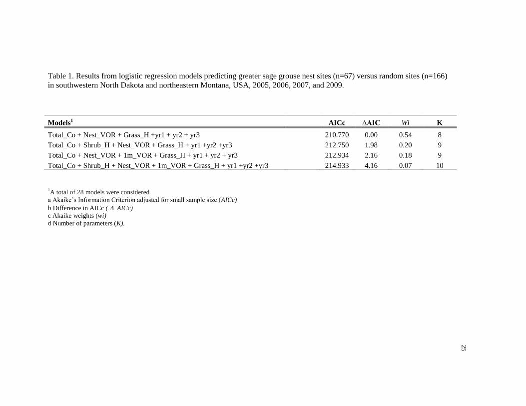
between 2005 and 2009. When I compared the 67 nest sites to the 166 random sites I

found that there were four competing models (Table 1). The best-approximating model

(AICc weight = 0.54) included total percent vegetation canopy cover, 0-m VOR, grass

height, and year affect. The top models indicated that the variables positively affected

resource selection for female sage grouse when choosing for a nest site. A second,

competing model included total percent vegetation canopy cover, average sagebrush

height and visual obstruction at 0-m. (AICc weight = 0.20).

Distributions of total percent vegetation canopy cover, sagebrush height, grass

height, visual obstruction 0-m, and visual obstruction at 1m differed (P <0.05) between

nest sites in 2005, 2006, 2007, and 2009 (Table 2). Visual obstruction at 0- m was

significant, thus having a positive affect on resource selection, all other variables were

not significantly different. Year effect was evident in data for random sites, therefore all

logistic models included the design variable year (Table 1). When I compared nest sites

to randomly generated sites I found the average vegetation measurements for nest sites

were larger than for random points (Figure 3). This indicates that nest sites were selected

because they had more suitable resources available compared to the randomly selected

sites.

16

Area of use versus area of avoidance

Once I identified the top models for predicting nest selection, I re-ran all 28 a-

priori models to develop the top models to predict vegetative resource selection within

the study area (Figure 4). When I compared the area of use sites to the area of avoidance

sites I found that there were four competing models; the best- approximating model

included total percent vegetation canopy cover and grass height (AICc weight = 0.25)

(Table 4). The variables in the top models indicated that the variables positively affected

resource selection for use and non-use areas, it indicates that total percent canopy cover

and grass height were two top factors in determining whether or not an area may be used

or avoided. A second competing model included total percent canopy cover, grass height

and visual obstruction at the 0- m mark(AICc weight = 0.19) both as positive correlates

of use.

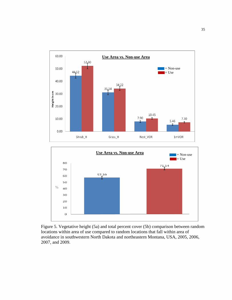
When comparing area of use to area of non-use, I found that in all comparisons

the average vegetation measurements within the area of use were larger (Figure 5). Thus

indicating that resource selection from female sage grouse favored taller vegetation and

higher percent canopy cover. Distributions of percent vegetation canopy cover, shrub

height, grass height, 0 m VOR, and 1 m VOR differed (P <0.05) between area of use

sites and area of avoidance sites in 2005, 2006, 2007, and 2009 (Table 3). Of the five

variables that were measured four ended up being significantly different, showing that

even though marginal resources were available in both areas (area of use vs. area of

avoidance) the resources that had more suitable resources (higher percent canopy cover

and taller vegetation) present were the areas chosen by sage grouse.

17

Road Density

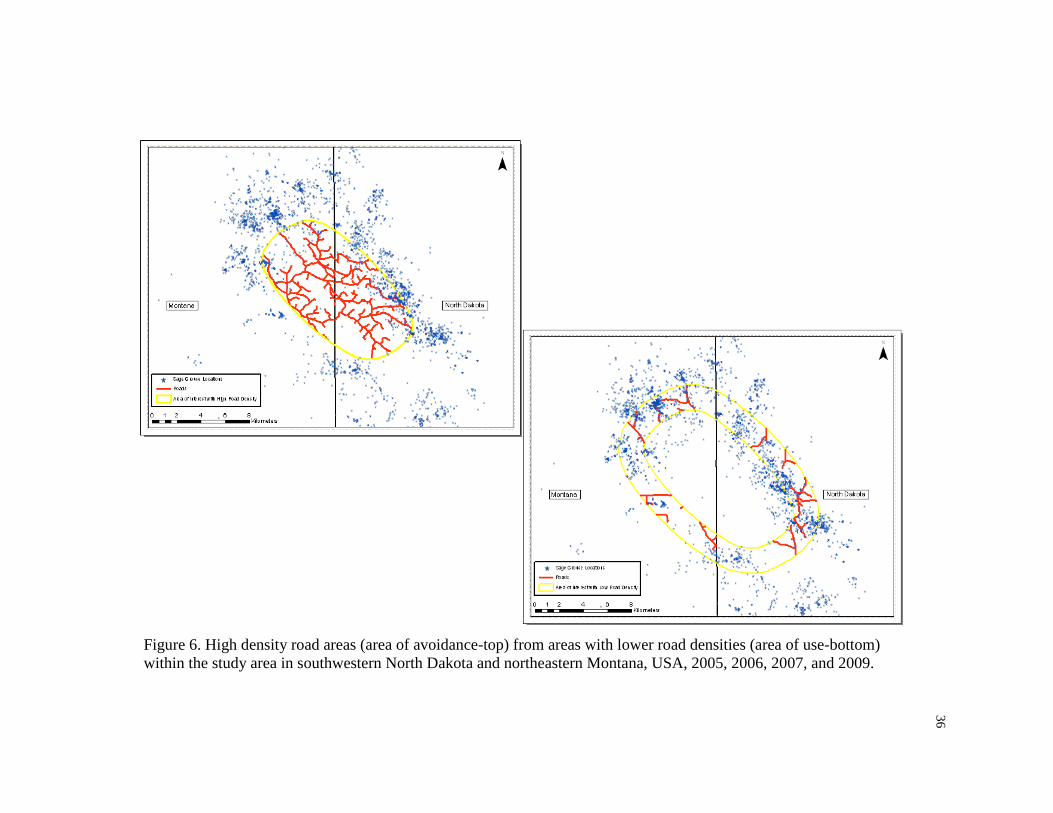
When I compared the area of avoidance (8,609.20 ha) to the area of use (8,609.20

ha; Figure 6), I found that the area of avoidance had 432 sage grouse locations compared

to 1,388 sage grouse locations within the area of use. When I compared density of roads I

found that the area of avoidance contained 120.9 km (0.0317 km/ha) of roads whereas the

area of use had 44 km (0.014 km/ha) of roads. Hence, the density of roads within the area

of avoidance was about 2.6 times greater than the density within the area of use (Figure

7).

Once I identified the top models for predicting nest site resource selection and

best models for determining vegetation differences between avoidance area and use area,

I re-ran the models to include a combination of all 56 a-priori models for comparison of

both nest site resource selection and for the area of avoidance and the area of use. The 56

a-priori models included 28 a-priori models without road density and 28 a-priori models

with road density. This was done to assess whether roads were a factor in resource

selection by sage grouse. Two different comparisons were made, the first comparison was

nest sites vs. random sites and the second comparison was made between use area vs.

non-use area. Road density was included with vegetative variables at randomly selected

sites (n=166) and compared to actual nest sites (n=67) this was the nest site vs. random

comparison. In addition, road density was also included with vegetative variables for the

comparison of area of use vs. area of non-use in this comparison random sites within the

area of use were compared to the area of non-use (use sites, n=69 and non-use sites

18

n=41); this was the second comparison indicating the differences between use area vs.

non-use areas.

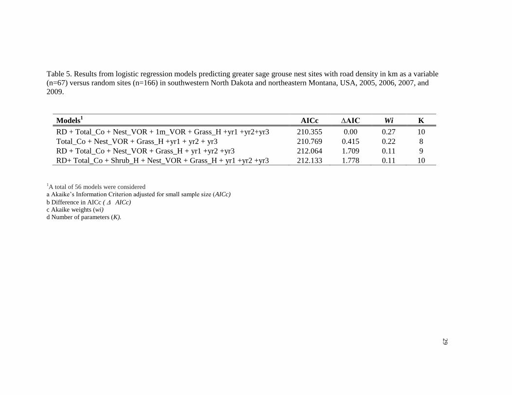
When looking at the nest site resource selection, the resulting models indicated

that there were four competing models. The best-approximating model (AICc weight =

0.27) included density of roads (km/ha), percent total canopy cover at the site level, VOR

at the 0-m mark, VOR at the 1-m mark, grass height, and year affect (Table 5). A second

model included percent total canopy cover at the site level, VOR at the 0-m mark, grass

height, and year affect (AICc weight = 0.22). Both top models revealed that each variable

within the model are important when it comes to the selection of resources; however, the

top model shows that road density plays a larger role in whether or not a sage grouse will

chose an area for nesting. When running these models the road density variable shifted to

the top of the models indicating that it is an important factor when sage grouse select a

nest area.

When looking at the area of use and the non-use area, the resulting models

indicated that there were four competing models. The best-approximating model (AICc

weight = 0.24) included density of roads (km/ha), percent total canopy cover at the site

level, and grass height (Table 6). A second model included density of roads (km/ha),

percent total canopy cover at the site level, VOR at the 0-m mark, and grass height (AICc

weight = 0.16). These models also indicate that road density play a major role in selection

of resources. These models illustrate that road density may be a major factor influencing

why an area may be avoided even when marginal resources are present.

19

Discussion

Resource Selection

Female sage grouse in North Dakota and Montana selected nest sites with higher

sagebrush cover and placed their nests beneath sagebrush plants which afforded greater

visual obstruction. Several studies have established the importance of sagebrush canopy

cover (Patterson 1952, Wallestad and Pyrah 1974, Wakkinen 1990, Fischer 1994, Sveum

et al. 1998) and herbaceous canopy cover (Wakkinen 1990, Connelly et al. 1991, Sveum

et al. 1998). In a previous study that took place in the same area, it was noted that sage

grouse nesting habitat, shrub density, and nest site VOR were also important predictors of

sage grouse nests (Herman-Brunson 2009). Connelly et al. (2000) recommended 15-25%

sagebrush canopy coverage for nesting sage grouse. I found that shrub height, grass

height, and nest site VOR also played an important and crucial role in resource selection.

In western North Dakota and eastern Montana, female sage grouse selected the best

available resources; however, in most cases these resources were marginal compared to

the recommendations from the core of the sage grouse range and sagebrush distribution.

In contrast to sagebrush, grass structure in North Dakota exceeded both management

recommendations (Connelly et al. 2000) and range-wide averages (Hagen et al. 2007).

Western North Dakota and eastern Montana forms a transition zone between the northern

wheatgrass-needlegrass prairie that dominates most of the Dakotas and the big sagebrush

plains of Wyoming (Johnson and Larson 1999). Thus, while North Dakota and Montana

appeared to have less than optimal sagebrush cover for sage grouse, the favorable grass

structure may have compensated for the sagebrush component. Both Herman-Brunson

20

(2007) in North Dakota,and Kaczor (2008) in a South Dakota study suggested that

despite low sagebrush density and canopy cover, the amount of grass cover around nests

suggests that grass was also an important cover component of sage grouse nests. Kaczor

(2008) also found grass structure was highly correlated with annual precipitation and in

periods of drought it may not provide adequate protection for sage grouse nests. Taller

live and residual grass surrounding nests also increased nest success in Alberta (Aldridge

and Brigham 2002), and was found to provide ample nest concealment in both sagebrush

and non-sagebrush over stories in Washington (Sveum et al. 1998). Sage grouse were

able to utilize grass cover for nest concealment in areas where sagebrush density and

height were suboptimal. However, there was still a requirement to maintain sagebrush on

the landscape because of its importance as a food source.

Across their range, female sage grouse usually select sagebrush patches with

percent shrub canopy cover of 15- 25% for nests. They generally avoid sparse or

excessively dense patches (Connelly et al. 2000). In southwestern North Dakota and

southeastern Montana, hens selected habitats with characteristics that offer marginal but

adequate cover, however they avoided high density road areas; this could be due to

habitat fragmentation or vehicle disturbance or a combination of both. Resources within

used areas had better overall vegetation structural quality when compared to avoided

areas with high road densities. Previous studies noted that hens selected nest sites with

the tallest available brush and which had the greatest stem diameter (Gray 1967,

Klebenow 1969, Wallestand and Pyrah 1974, Autenreith 1981). Herman-Brunson (2007)

found that hens did not select for taller sagebrush at nests. Herman-Brunson (2007) also

21

stated that sage grouse can inhabit areas of lower sagebrush height and density than

reported in existing literature, if additional cover in the form of graminoids are available.

Previous studies have also documented the importance of cover from grasses within

shrub stands (Wakkinen 1990, Connelly et al. 1991, and Kaczor et al. 2011) which are

associated with higher nest success rates (Gregg et al. 1994), and can offer additional nest

protection. When directing our attention to the area of avoidance verses the area of use I

found nine nest locations that fell within the area of avoidance and 26 nest locations that

fell within the area of use.

When I compared the area of avoidance and area of use there was a noticeable

difference in vegetation means, differences between vegetation showed to be significant

in most cases when comparing the area of use to the area of avoidance. The area of use

had taller vegetation and had higher percent cover then that of the non-use area making

the area of use more appealing for the utilization of resources. However, the area of

avoidance vegetation means still fell within marginal habitat requirements within the

published literature (Connelly et al. 2000, Hagen et al. 2007). Because of this, I examined

other influencing factors, and chose road density because it was a logical indicator of the

intensity of oil and gas development within the area. When I included road density into

the vegetative models of resource selection, the road density variable became a variable

that was present in all of the top-rated models. This suggested that road density was a key

factor in resource selection.

To date no studies have specifically investigated road density effects on sage

grouse populations. Studies do suggest that some sage grouse population declines are

22

related to the loss or fragmentation of habitat caused by oil and gas site preparation, road

development, noise from pumping stations, power line development, and associated

human activities (Braun 1987). Within the Cedar Creek Anticline, male abundance at

leks decreased by 52 percent at sixteen leks with more than one well pad per 2.6 square

kilometers within 3.2 kilometers, and no males were counted in 2009 at four of the

sixteen impacted leks that had multiple displaying males in 2008 (Tack 2009). Energy

development is also known to impact wildlife directly by altering habitat use (Doherty et

al. 2008). Because the area avoided by radio-marked sage grouse had a higher density of

roads than the area of more intense use; hence the density of roads may be contributing to

the avoidance in this area. Additionally, higher road densities lead to greater

fragmentation of the landscape, thereby reducing its value as habitat for sage grouse.

23

Management Implications and Future Research Needs

Sage grouse in the United States are listed as a candidate for listing under the

Endangered Species Act. In 2010, after a second review, the Department of the Interior

assigned the sage grouse status as "warranted but precluded”. If sage grouse populations

continue to decline and shrink in distribution, sagebrush steppe conservation and

enhancement could be top a priority for land management agencies. Particularly, efforts

to conserve the limited range of sagebrush within southwestern North Dakota and

southeastern Montana will be vital to maintaining sage grouse populations.

Management for greater grass cover and height, reduced conversion to tillage

agricultural, and minimizing habitat fragmentation from activities such as energy

development could be a goal for resource managers. In addition, annual grazing

utilization should not exceed 35% in order to improve rangeland conditions, particularly

to maintain sagebrush cover (Holechek et al. 1999). I suggest that managers develop

strategies to preserve the integrity of sagebrush steppe in southwestern North Dakota and

southeastern Montana. Range management practices that could increase sagebrush and

grass cover and height might include: rest-rotation grazing, where the pasture is not

grazed until early July to allow for undisturbed nesting, or reduced grazing intensities

and/or season of use to reduce impact on sagebrush and grass growth (Adams et al.

2004). I would also recommend against using prescribed fire in areas with sagebrush, it is

documented that Wyoming big sagebrush typically takes 50-120 years to recover from a

fire (Baker 2006).

24

Oil and gas development creates a complex network of roads, well pads,

pipelines, pumping stations, and other infrastructure features across a landscape. Roads

are widely recognized by the scientific community as having a variety of direct, indirect,

and cumulative effects on wildlife and their habitats (Trombulak and Frissell 2000,

Gucinski et al. 2001, Gaines et al. 2003, Wisdom et al. 2004a, Wisdom et al. 2004b, New

Mexico Department of Game and Fish 2005). Increasingly, studies have demonstrated

many of the negative effects of oil and gas developments specific to wildlife populations

(Colorado Department of Wildlife et al. 2008, Wyoming Game and Fish Department

2004, Confluence Consulting 2005, Holloran 2005, Sawyer et al. 2006, Berger et al.

2006). This study illustrates that road density could be a key factor influencing sage

grouse avoidance of potentially useable habitats, particularly when the vegetative

characteristics within those habitats may be marginal at the onset. However, additional

research is needed to understand the specific boundaries and standards that must be set to

maintain the integrity of sagebrush steppe resources.

Because sage grouse have not been listed on the Endangered Species Act it is

imperative to have long-term (>30 yrs) partnerships and quality incentives for local land

owners. This will require cooperation from state wildlife agencies, federal land

management agencies, local natural resource conservation districts, and committed

landowners. Private landowners should be encouraged to participate in programs that are

directed at maintaining and improving sage grouse habitats on private lands. Good

working relationships and good education about sage grouse and their resource

requirements is a key component for their success.

25

Table 1. Results from logistic regression models predicting greater sage grouse nest sites (n=67) versus random sites (n=166)

in southwestern North Dakota and northeastern Montana, USA, 2005, 2006, 2007, and 2009.

1A total of 28 models were considered

a Akaike’s Information Criterion adjusted for small sample size (AICc)

b Difference in AICc ( AICc)

c Akaike weights (wi)

d Number of parameters (K).

Models1 AICc ∆AIC Wi K

Total_Co + Nest_VOR + Grass_H +yr1 + yr2 + yr3 210.770 0.00 0.54 8

Total_Co + Shrub_H + Nest_VOR + Grass_H + yr1 +yr2 +yr3 212.750 1.98 0.20 9

Total_Co + Nest_VOR + 1m_VOR + Grass_H + yr1 + yr2 + yr3 212.934 2.16 0.18 9

Total_Co + Shrub_H + Nest_VOR + 1m_VOR + Grass_H + yr1 +yr2 +yr3 214.933 4.16 0.07 10

25

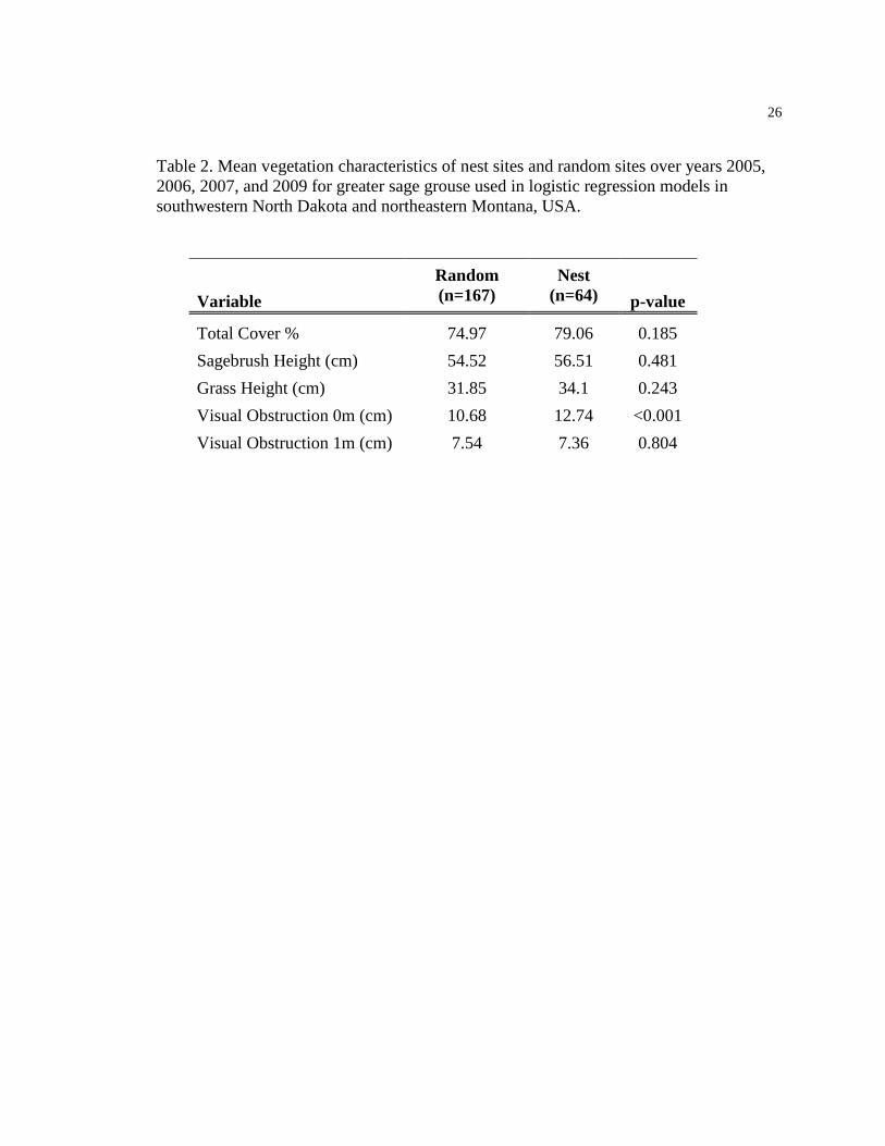
26

Table 2. Mean vegetation characteristics of nest sites and random sites over years 2005,

2006, 2007, and 2009 for greater sage grouse used in logistic regression models in

southwestern North Dakota and northeastern Montana, USA.

Variable

Random

(n=167)

Nest

(n=64) p-value

Total Cover % 74.97 79.06 0.185

Sagebrush Height (cm) 54.52 56.51 0.481

Grass Height (cm) 31.85 34.1 0.243

Visual Obstruction 0m (cm) 10.68 12.74 <0.001

Visual Obstruction 1m (cm) 7.54 7.36 0.804

27

Table 3. Mean vegetation characteristics of random points inside area of use and random

sites in area of avoidance over years 2005, 2006, 2007, and 2009 for greater sage grouse

used in logistic regression models in southwestern North Dakota and northeastern

Montana, USA.

Area Inside (n=41) Area Outside (n=69)

Variable Mean SE Mean SE p-vale

Total_Co 57.39 3.42 71.54 2.46 <0.001

Shrub_Height 44.52 2.08 52.30 2.26 0.02

Grass_Height 31.14 1.94 34.22 1.48 0.21

0m_VOR 7.90 0.69 10.45 0.60 0.01

1m_VOR 5.46 0.65 7.30 0.52 0.03

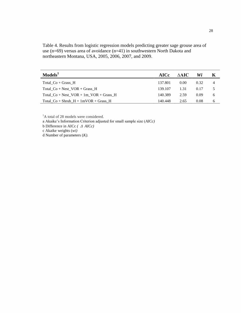
28

Table 4. Results from logistic regression models predicting greater sage grouse area of

use (n=69) versus area of avoidance (n=41) in southwestern North Dakota and

northeastern Montana, USA, 2005, 2006, 2007, and 2009.

Models1

AICc ∆AIC Wi K

Total_Co + Grass_H 137.801 0.00 0.32 4

Total_Co + Nest_VOR + Grass_H 139.107 1.31 0.17 5

Total_Co + Nest_VOR + 1m_VOR + Grass_H 140.389 2.59 0.09 6

Total_Co + Shrub_H + 1mVOR + Grass_H 140.448 2.65 0.08 6

1A total of 28 models were considered.

a Akaike’s Information Criterion adjusted for small sample size (AICc)

b Difference in AICc ( AICc)

c Akaike weights (wi)

d Number of parameters (K).

29

Table 5. Results from logistic regression models predicting greater sage grouse nest sites with road density in km as a variable

(n=67) versus random sites (n=166) in southwestern North Dakota and northeastern Montana, USA, 2005, 2006, 2007, and

2009.

Models1

AICc ∆AIC Wi K

RD + Total_Co + Nest_VOR + 1m_VOR + Grass_H +yr1 +yr2+yr3 210.355 0.00 0.27 10

Total_Co + Nest_VOR + Grass_H +yr1 + yr2 + yr3 210.769 0.415 0.22 8

RD + Total_Co + Nest_VOR + Grass_H + yr1 +yr2 +yr3 212.064 1.709 0.11 9

RD+ Total_Co + Shrub_H + Nest_VOR + Grass_H + yr1 +yr2 +yr3 212.133 1.778 0.11 10

1A total of 56 models were considered

a Akaike’s Information Criterion adjusted for small sample size (AICc)

b Difference in AICc ( AICc)

c Akaike weights (wi)

d Number of parameters (K).

29

30

Table 6. Results from logistic regression models predicting greater sage grouse nest sites

with road density in km as a variable (n=41) versus random sites (n=69) in southwestern

North Dakota and northeastern Montana, USA, 2005, 2006, 2007, and 2009.

Models AICc ∆AIC Wi K

RD + Total_Co + Grass_H 132.181 0.00 0.24 5

RD+ Total_Co + Nest_VOR + Grass_H 132.968 0.79 0.16 6

RD +Total_Co + Nest_VOR + 1m_VOR + Grass_H 133.438 1.26 0.13 7

RD+ Total_Co + Shrub_H + 1mVOR + Grass_H 133.518 1.34 0.12 7

1A total of 56 models were considered

a Akaike’s Information Criterion adjusted for small sample size (AICc)

b Difference in AICc ( AICc)

c Akaike weights (wi)

d Number of parameters (K).

31

Figure 1. Study area of Bowman and Slope counties, North Dakota and Fallon County,

Montana with vegetation sample locations documented during 2005, 2006, 2007, and

2009. The dashed area shows current range and green area shows historic range

(Schroeder et al. 2004).

32

Figure 2. Demonstration of intersect method used and highlights a 350M buffer area and

a portion of the road segment for better understanding.

33

Figure 3. Vegetative height (3a) and total percent cover (3b) comparison between nest

sites and random points in southwestern North Dakota and northeastern Montana, USA,

2005, 2006, 2007, and 2009.

= Random

= Nest

= Random

= Nest

34

Figure 4. Sage grouse locations from previous work (Swanson, 2009 Herman-Brunson

2007) along with random selected vegetation sampled locations and nest sites. Area of

avoidance circled in yellow and area of use circled in green in southwestern North

Dakota and northeastern Montana, USA, 2005, 2006, 2007, and 2009.

35

Figure 5. Vegetative height (5a) and total percent cover (5b) comparison between random

locations within area of use compared to random locations that fall within area of

avoidance in southwestern North Dakota and northeastern Montana, USA, 2005, 2006,

2007, and 2009.

%

Use Area vs. Non-use Area

Use Area vs. Non-use Area

= Non-use

= Use

= Non-use

= Use

35

Figure 6. High density road areas (area of avoidance-top) from areas with lower road densities (area of use-bottom)

within the study area in southwestern North Dakota and northeastern Montana, USA, 2005, 2006, 2007, and 2009.

36

37

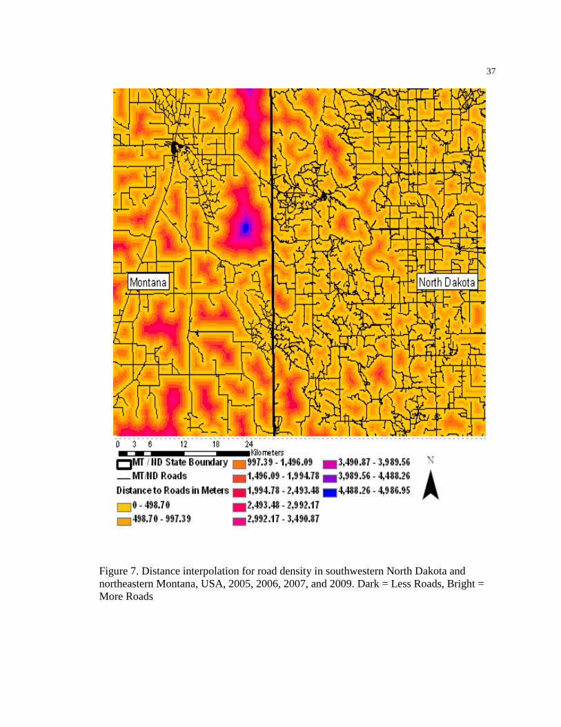
Figure 7. Distance interpolation for road density in southwestern North Dakota and

northeastern Montana, USA, 2005, 2006, 2007, and 2009. Dark = Less Roads, Bright =

More Roads

38

Literature Cited

Adams, B. W., J. Carlson, D. Milner, T. Hood, B. Cairns, and P. Herzog. 2004.

Beneficial grazing management practices for sage-grouse (Centrocercus

urophasianus) and ecology of silver sagebrush (Artemisia cana) in southeastern

Alberta.

Aldridge CL, SE Nielsen, HL Beyer, MS Boyce, JW Connelly, ST Knick, and MA

Schroeder. 2008. Range-wide patterns of greater sage-grouse persistence.

Diversity and Distributions 14(6):983–994.

Autenrieth, R. E. 1981. Sage Grouse management in Idaho. ID Dept. Fish Game, Boise.

Wildlife Bulletin.

Baker, W. L. 2006. Fire and restoration of sagebrush ecosystems. Wildlife Society

Bulletin 34:177-185.

Benkobi, L., D. W. Uresk, G. Schenbeck, and R. M. King. 2000. Protocol for monitoring

standing crop in grasslands using visual obstruction. Journal of Range

Management 53:627-633.

Berger, J., K.M. Berger, and J.P. Beckmann. 2006. Wildlife and energy development:

Pronghorn of the Upper Green River Basin – Year 1 Summary. Wildlife

Conservation Society, Bronx, NY. Available at:

http://www.wcs.org/media/file/Shell%20Year%201%20Progress%20III.pdf.

Bergquist, E., P. Evangelista, T. J. Stohlgren, and N. Alley. 2007. Invasive species and

coal bed methane development in the Powder River Basin, Wyoming.

Environmental Monitoring & Assessment 128:381-394.

39

Braun, C. E. 1987. Current issues in sage grouse management. Western Association of

Fish and Wildlife Agencies: Proceedings 67:134-144.

Braun, C. E. 1998. Sage grouse declines in western North America: What are the

problems? Western Association of Fish and Wildlife Agencies: Proceedings

78:139-156.

Braun, C. E., O. O. Oedekoven, and C. L. Aldridge. 2002. Oil and gas development in

western North America: Effects on sagebrush steppe avifauna with particular

emphasis on Sage grouse. North American Wildlife and Natural Resources

Conference Transactions 67:337-349.

Burnham, K. P., and D.R. Anderson. 2002. Model selection and multimodel inference: a

practical information-theoretic approach. Second edition. Springer-Verlag, New

York, New York, USA.

Colorado Department of Wildlife,Wildlife and Parks, North Dakota Game and Fish, Utah

Division of Wildlife Resources, and Wyoming Game and Fish Department. 2008.

Using the Best Available Science to Coordinate Conservation Actions that Benefit

Greater Sage-Grouse Across States Affected by Oil & Gas Development in

Management Zones I-II (Colorado, Montana, North Dakota, South Dakota, Utah,

and Wyoming). (Unpublished report, available at

http://www.ourpubliclands.org/files/upload/BestScience_2008_sagegrouse_energ

y.pdf.).

Connelly, J. W., and C. E. Braun. 1997. Long-term changes in Sage Grouse populations

in western North America. Wildlife Biology 3:229-234

40

Connelly, J.W. S.T. Knick, M.A. Schroeder, and S.J. Stiver. 2004. Conservation

assessment of greater sage-grouse and sagebrush habitats. Western Association

of Fish and Wildlife Agencies. Unpublished Report. Cheyenne, Wyoming.

Connelly, J.W., M.A. Schroeder, A.R. Sands, and C.E. Braun. 2000. Guidelines

to manage sage grouse populations and their habitats. Wildlife Society Bulletin

28:1-19.

Connelly, J. W., W. L. Wakkinen, A. D. Apa, and K. P. Reese. 1991. Sage grouse use of

nest sites in southeastern Idaho. Journal of Wildlife Management 55:521-524.

Consulting, Inc. 2005. Annotated Bibliography of potential impacts of gas and oil

exploration and development on coldwater fisheries. Prepared by Confluence

Consulting, Inc., for Trout Unlimited, Bozeman, MT.

Cottam, G., and J. T. Curtis. 1956. The use of distance measures in phytosociological

sampling. Ecology 37:451-460.

Crawford, J. A. 1997. Importance of herbaceous vegetation to female sage grouse

Centrocercus urophasianus during the reproductive period: A synthesis of

research from Oregon, USA. Wildlife Biology.

Daubenmire, R. 1959. A canopy-coverage method of vegetational analysis. Northwest

Science 33:43-62.

Doherty, K. E., D. E. Naugle, B. L. Walker, and J. M. Graham. 2008. Greater sage-

grouse winter habitat selection and energy development. Journal of Wildlife

Management 72:187-195.

43

Doherty, M. K. 2007. Mosquito populations in the Powder River Basin, Wyoming: a

comparison of natural, agricultural and effluent coal-bed natural gas aquatic

habitats. M. S. Thesis., Montana State University Bozeman, Montana, USA.

Drut, M. S., A. C. John, and A. G. Michael. 1994. Brood habitat use by sage grouse in

Oregon. Great Basin Naturalist 54:170-176.

Ellis, K. L. 1984. Behavior of a lekking sage grouse in response to a perched golden

eagle. Western Birds 15:37-38.

Ellis, K. L. 1987. Effects of a new transmission line on breeding male greater sage-grouse

at a lek in northwestern. Western Association of Fish and Game Agencies,

Midway, Utah, USA.

Fischer, R. A. 1994. The effects of prescribed fire on the ecology of migratory sage

grouse in southeastern Idaho. PhD Dissertation. Univ. ID.

Fischer, R. A., J. W. Connelly, K. P. Reese, W. L. Wakkinen, and A. D. Apa. 1993.

Nesting-area fidelity of sage grouse in southeastern Idaho The Condor 95:1038-

1041.

Fischer, R. A., K. P. Reese, and J. W. Connelly. 1996. Influence of vegetal moisture

content and nest fate on timing of female sage grouse migration. Condor 98:868-

872.

Gaines, W. L., P. H. Singleton, and R. C. Ross. 2003. Assessing the cumulative

effects of linear recreation routes on wildlife habitats on the Okanogan and

Wenatchee National Forests., U.S. Department of Agriculture, Forest Service,

General Technical Report PNW-GTR-586. Portland, Oregon USA.

41

42

43

Giesen, K.M., T.J. Schoenberg, and C.E. Braun. 1982. Methods for trapping Sage Grouse

in Colorado. Wildlife Society Bulletin 10:224-231.

Gill, R.B. 1966. A literature review on sage grouse. Colorado Game, Fish, and Parks,

Research Division and Cooperative Wildlife Research Unit, Denver, Colorado,

USA.

Graul, W. D. 1980. Grassland management practices and bird communities.

Gray, G.M. 1967. An ecological study of Sage Grouse broods with reference to nesting,

movements, food habits, and sagebrush strip-spraying in the Medicine Lodge

Drainage, Clark County, Idaho. M.S. Thesis. Univ. ID, Moscow. 200pp.

Gregg, M. A., and J. A. Crawford. 1994. Vegetational cover and predation of sage grouse

nest in Oregon. Journal of Wildlife Management 58:162-166.

Gucinski, H., M. H. Brookes, M. J. Furniss, R. R. Ziemer, and M. Brookes. 2001. Forest

roads: a synthesis of scientific information.

Hagen, C. A., J. W. Connelly, and M. A. Schroeder. 2007. A meta-analysis of greater

sagegrouse Centrocercus urophasianus nesting and brood-rearing habitats.

Wildlife Biology:13: 42-50.

Hemstrom, M. A., M. J. Wisdom, W. J. Hann, M. M. Rowland, B. C. Wales, and R. A.

Gravenmier. 2002. Sagebrush-Steppe vegetation dynamics and restoration

potential in the Interior Columbia Basin, U.S.A. Conservation Biology 16:1243-

1255.

Herman-Brunson, K. M. 2007. Nesting and brood-rearing habitat selection of Greater

Sage Grouse and associated survival of hens and broods at the ddge of their

43

historic distribution. M.S. Thesis, South Dakota State University, Brookings, SD,

USA.

Herman-Brunson, K.M., Jensen, K.C., Kaczor, N.W., Swanson, C.C., Rumble, R.A.,

Klaver, R.W. 2009. Nesting ecology of greater sage-grouse Centrocercus

urophasianus at the eastern edge of their historic distribution. Wildlife Biology.

Holechek, J. L., G. Hilton, F. Molinar, and D. Galt. 1999. Grazing Studies: What We've

Learned. Rangelands 21:12-16.

Holloran, M. J. 2005. Greater sage-grouse (Centrocercus urophasianus) population

response to natural gas field development in western Wyoming. PhD Dissertation,

University of Wyoming, Laramie, USA.

Homer, C. G., and T. C. Edwards Jr. 1993. Use of remote sensing methods in modelling

sage grouse winter habitat. Journal of Wildlife Management 57:78-84.

Hosmer, D. W., S. Lemeshow. 2000. Applied logistic regression, 2nd Edition. John

Wiley & Sons Incorporated Publication, New York, New York USA.

Hupp, J. W., and E. B. Clait. 1989. Topographic distribution of Sage Grouse foraging in

winter. Journal of Wildlife Management 53:823-829

Johnson, J. R., and G. E. Larson. 1999. Grassland plants of South Dakota and the

northern Great Plains. South Dakota State University, Brookings, South Dakota,

USA.

Johnson, P. R. 1976. Soil Survey of Butte County, South Dakota. U.S. Department

Agriculture Soil Conservation Service. Soil Survey.

43

Kaczor, N. W. 2008. Nesting and brood-rearing success and resource selection of greater

sage-grouse in northwestern South Dakota. M.S. Thesis, South Dakota State

University, Brookings, SD, USA.

Kaczor, N.W, Jensen, K.C., Klaver, R.W., Rumble M.A., Herman-Brunson K.M.,

Swanson C.C. 2011.Nesting success and resource selection of greater sage-

grouse. Ecology, Conservation, and Management of Grouse. In press.

Klebenow, D. A. 1969. Sage grouse nesting and brood habitat in Idaho. The Journal of

Wildlife Management 33:649-662.

Lyon, A. G., and S. H. Anderson. 2003. Potential gas development impacts on sage

grouse nest initiation and movement. Wildlife Society Bulletin 31:486-491.

Musil, D. D., P. R. Kerry, and W. C. John. 1994. Nesting and summer habitat use by

translocated sage grouse (Centrocercus Urophasianus) in Central Idaho. Great

Basin Naturalist 54:228-233.

Naugle, D. E., B. L. Walker, and K. E. Doherty. 2006. Sage-grouse population response

to coal-bed natural gas development in the Powder River Basin: interim progress

report on region-wide lek-count analyses. Unpublished Report, University of

Montana, Missoula, USA.

Naugle, D. E., K.E. Doherty, B. L. Walker, M. J. Holloran, and H. E. Copeland. 2011.

Energy development and sage-grouse. Number 21 in S.T. Knick and J.W.

New Mexico Department of Game and Fish. 2005. Habitat fragmentation and the effects

of roads on wildlife and habitats. Available at:

43

http://www.wildlife.state.nm.us/conservation/habitathandbook/documents/2004Ef

fectsofRoadsonWildlifeandHabitats.pdf.

Opdahl, D. D. 1975. Soil survey of Bowman County, North Dakota. U.S. Department

Agriculture Soil Conservation Service Soil Survey.

Patterson, R. L. 1952. The sage grouse in Wyoming. Denver, CO, USA.

Plumpton, D. L., and D. E. Andersen. 1997. Habitat use and time budgeting by wintering

ferruginous hawks. Condor 99:888-905.

Paige, C., and S.A. Ritter. 1999. Birds in a sagebrush sea: managing sagebrush habitats

for bird communities. Partners in Western Flight working Group, Boise, ID.

Robel, R. J., J. N. Briggs, A. D. Dayton, and L. C. Hulbert. 1970. Relationships between

visual obstruction measurements and weight of grassland vegetation. Journal of

Range Management 23:295-297.

Sargeant, A. B., M. A. Sovada, and R. J. Greenwood. 1998. Interpreting evidence of

depredation of duck nests in the prairie pothole region.

Sawyer, H., R. M. Nielson, F. Lindzey, and L. L. McDonald. 2006. Winter habitat

selection of mule deer before and during development of a natural gas field.

Journal of Wildlife Management 70:396-403.

Schroeder, M. A., L. A. Cameron, A. D. Apa, J. R. Bohne, C. E. Braun, S. D. Bunnell, J.

W. Connelly, P. A. Deibert, S. C. Gardner, M. A. Hilliard, G. D. Kobriger, S. M.

McAdam, W. M. Clinton, J. J. McCarthy, L. Mitchell, E. V. Rickerson, and S. J.

Stiver. 2004. Distribution of Sage-Grouse in North America. The Condor

106:363-376.

46

Schroeder, M.A., J.R. Young, and C.E. Bruan. 1999. Sage grouse (Centrocercus

urophasianus). Pages 1-28 in A. Poole and F. Gill, editors. The birds of North

America, No. 425. The Birds of North America, Inc., Philadelphia, Pennsylvania,

USA.

Scott, J. W. 1942. Mating behavior of the sage grouse. The Auk 59:477-498.

Smith, J. 2003. Greater sage-grouse on the edge of their range: leks and surrounding

landscapes in the Dakotas. M.S. Thesis, South Dakota State University,

Brookings, South Dakota, USA.

Sorensen, T., P. D. McLoughlin, D. Hervieux, E. Dzus, J. Nolan, B. O. B. Wynes, and S.

Boutin. 2008. Determining sustainable levels of cumulative effects for boreal

caribou. Journal of Wildlife Management 72:900-905.

Sveum, C. M., W. D. Edge, and J. A. Crawford. 1998. Nesting habitat selection by sage

grouse in south-central Washington. Journal of Range Management 51:265-269.

Swanson, C. 2009. Ecology of greater sage-grouse in the Dakotas. PhD. Dissertation,

South Dakota State University, Brookings, SD, USA.

Swenson, J. E., A. S. Claire, and D. E. Charles. 1987. Decrease of Sage Grouse

(Centrocercus Urophasianus) after ploughing of sagebrush steppe. Biological

Conservation 41.

Tack, J. E. 2009. Sage-grouse and the human footprint: Implications for conservation of

small and declining populations. M.S. thesis, University of Montana, Missoula.

43

Thompson, K. W. 1978. Soil Survey of Slope County, North Dakota. U.S. Department of

Agriculture, Soil Conservation Service and Forest Service, North Dakota

Agricultural Experiment Station, Fargo, North Dakota, USA.

Trombulak, S. C., and C. A. Frissell. 2000. Review of ecological effects of roads on

terrestrial and aquatic communities. Conservation Biology 14:18-30.

Wakeley, J. S. 1978. Hunting methods and factors affecting their use by ferruginous

hawks. Condor 80:327-333.

Wakkinen, W. L. 1990. Nest site characteristics and spring-summer movements of

migratory sage grouse in southeastern Idaho. M. S. Thesis, University of Idaho,

Moscow, USA.

Walker, B. L., D. E. Naugle, and K. E. Doherty. 2007. Greater sage-grouse population

response to energy development and habitat loss. Journal of Wildlife Management

71:2644-2654.

Wallestad, R. 1975. Life history and habitat requirements of sage grouse in central

Montana. Montana Department of Fish and Game.

Wallestad, R., and D. Pyrah. 1974. Movement and nesting of sage grouse hens in central

Montana. The Journal of Wildlife Management 38:630-633.

Welch, B. L., J. W. Fred, and A. R. Jay. 1991. Preference of wintering sage grouse for

big sagebrush. Journal of Range Management 44:462-465.

47

Wisdom, M. J., A. A. Ager, H. K. Preisler, N. J. Cimon, and B. K. Johnson. 2004a.

Effects of off-road recreation on mule deer and elk. Transactions of the North

American Wildlife and Natural Resources Conference 69:531-550.

Wisdom, M. J., N. J. Cimon, B. K. Johnson, E. O. Garton, and J. W. Thomas. 2004b.

Spatial partitioning by mule deer and elk in relation to traffic. Transactions of the

North American Wildlife and Natural Resources Conference 69:509-530.

Wrobleski, D. W., and J. B. Kauffman. 2003. Initial effects of prescribed fire on

morphology, abundance, and phenology of forbs in big sagebrush communities in

southeastern Oregon. Restoration Ecology 11:82–90.

Wyoming Game and Fish Department., 2004. Recommendations for development of oil

and gas resources within crucial and important wildlife habitat: A strategy for

managing energy development consistently with the FLPMA Principles of

multiple use and sustained yield. Available at

http://gf.state.wy.us/downloads/pdf/og.pdf.

Zou, L., S. N. Miller, and E. T. Schmidtmann. 2006. Mosquito larval habitat mapping

using remote sensing and GIS: implications of coalbed methane development and

West Nile virus. Journal of Medical Entomology 43:1034-1041.

Zou, L., S. N. Miller, and E. T. Schmidtmann. 2007. A GIS tool to estimate West Nile

virus risk based on a degree-day model. Environmental Monitoring & Assessment

129:413-420.