mantle plume tomography - richard...

(2007) 248–263www.elsevier.com/locate/chemgeo

Chemical Geology 241

Mantle plume tomography

Guust Nolet a, Richard Allen b, Dapeng Zhao c,⁎

a Department of Geosciences, Princeton University, Princeton, NJ 08544, United Statesb Department of Earth and Planetary Science, University of California, Berkeley, CA 94720, United States

c Geodynamics Research Center, Ehime University, Matsuyama 790–8577, Japan

Accepted 22 January 2007

Abstract

We review the resolution currently available with seismic tomography, in particular the ability of seismic waves to image mantleplumes, and discuss frequently asked questions about artifacts, interpretation and possible systematic errors. These aspects arediscussed in more detail for two case histories offering different problems in the tomographic interpretation: Iceland and Hawaii.Regional and global models resolve a vertical low velocity anomaly beneath Iceland, interpreted as an upwelling, from thetransition zone up to the base of the lithosphere. Beneath the transition zone any continuation of the low-velocity anomaly is weakat best. This may be due to the absence of such an anomaly, poor seismic resolution in the lower mantle, or the weak sensitivity ofvelocity to buoyancy at these depths. While we are confident of the presence of a plume in the upper mantle, its origins remain tobe resolved. Because of its large distance to most seismic sources and stations, the mantle structure under Hawaii is among the mostdifficult to image tomographically, but several recent global tomography studies agree on a whole-mantle plume under theHawaiian hotspot. The plume exhibits a tilting geometry, which is likely due to the mantle flow. Theoretical advances, as well asdeployments of large seismic networks across hotspot regions, are expected to bring significant improvements to the imaging ofnarrow mantle upwellings in the near future.© 2007 Elsevier B.V. All rights reserved.

Keywords: Seismic tomography; Mantle plumes; Upper mantle; Lower mantle

1. Introduction

Seismologists have known for a long time how tointerpret the arrival times of seismic waves to determinethe time and location of earthquakes as well as thevariation of seismic wavespeed with depth. In the 20thcentury, such layered Earth models were subject to everincreasing refinements until it became evident that a

⁎ Corresponding author. Present address: Department of Geophysics,Tohoku University, Sendai, Japan.

E-mail addresses: [email protected] (G. Nolet),[email protected] (D. Zhao).

0009-2541/$ - see front matter © 2007 Elsevier B.V. All rights reserved.doi:10.1016/j.chemgeo.2007.01.022

simple depth-dependence of seismic velocities wasinsufficient to explain the remaining discrepanciesbetween observed and predicted arrival times. In thefootsteps of medical tomography, where radiologistsbegan to use computers to obtain X ray scans that focuson a plane of interest, two pioneering groups at MIT andHarvard obtained the first seismological tomograms ofthe Earth's interior by mapping anomalies in thecompressional seismic velocity Vp (Aki and Lee,1976; Dziewonski et al., 1977).

Whereas a medical CAT-scan is obtained by illumi-nating the body from all angles, the seismological scanis much more primitive: it is constructed from a finite

mailto:[email protected]


http://dx.doi.org/10.1016/j.chemgeo.2007.01.022

249G. Nolet et al. / Chemical Geology 241 (2007) 248–263

number of sources (earthquakes and occasionallynuclear test explosions) and an even more limitednumber of receivers. Worse, most of the receivers arelocated on land, leaving the oceanic areas largelyuncovered. The fact that the seismic waves followpaths that are not straight, and that the wavelengths ofseismic waves are of the same order as the scale lengthof the heterogeneities we wish to image adds anotherlevel of complexity. Notwithstanding these difficulties,the method of seismic tomography has blossomed nearthe end of the twentieth century: improvements in thetheory of interpretation, expanding networks of high-quality stations with broadband response, and a highdegree of cooperation through international data centers(IRIS in the US and ORFEUS in the Netherlands) led toever increasing detail of global tomographic models.

Since plate boundaries dominate the global seismic-ity, it comes as no surprise that subduction zones areeasier to image than anomalies elsewhere; in particular,their counterpart in the mantle flow – plumes – aresupposedly narrow, away from seismically active areas,therefore difficult to image. A breakthrough in slabtomography was the discovery that many oceanic platesare able to penetrate the 670 km discontinuity (van derHilst et al., 1991). This finding has been widelyinterpreted as evidence for ‘whole mantle convection’,though that may turn out to be somewhat of an over-interpretation, and the exact nature of the return flowremains elusive. Yet mass flux through the 670discontinuity must be balanced either by a return flow,or by a change in the depth of the 670 discontinuity. Inthe latter case, the changed T–P conditions at the phaseboundary will eventually return the discontinuity to thedepth dictated by the phase equilibrium, thus providing ahidden return flow that has little to do with the concept ofwhole-mantle convection. In the case where the returnflow is explicit, its character remains to be determined.Davies (1998) favors a distributed flow, with indepen-dent return flows for plumes and slabs. This view is inagreement with the very low contribution of the plumeheat flux to the total heat flux of the Earth as inferredfrom dynamic topography (Sleep, 1990; Davies, 1990).However, Bunge (2005) argues that the geotherm issubadiabatic, leading to an underestimate for deep heatflux from surface buoyancy, and advocates a larger rolefor plumes in heat transport. Nolet et al. (2006) reach asimilar conclusion from early tomographic images ofmantle plumes. Clearly, it has become important not justto obtain images of plumes but also to get reliableinformation on their size, shape and temperatureanomaly. In this paper we take stock of the presentstate of affairs of plume imagery.

2. Plume images in recent tomography

Until recently, seismic tomography provided littledirect evidence for lower mantle plumes. The existenceof the African and Pacific ‘superplumes’ – vast piles ofmaterial with lowered seismic velocity and probably ahigher density – was uncontested (e.g. Romanowicz andGung, 2002), but as recently as 2003 Ritsema and Allenconcluded: “Whole-mantle plumes are well establishedthrough both numerical and analog experiments, butconclusive evidence for their existence remains elusive onEarth” (Ritsema andAllen 2003). At that time the first, stilltentative, images of plumeswere appearing in the literature(Bijwaard and Spakman, 1999; Goes et al., 1999; Zhao,2001; Rhodes and Davies, 2001), but agreement betweendifferent models was poor. One of the major hurdles is the(presumed) narrow conduit of plumes, which makes iteasy for seismic waves to diffract around them, thusmasking any delay acquired by the wave energy thatactually travels through the plume by earlier arrivals thathave found a way around the low velocities.

More recently, a new approach to seismic inversionthat compensates for the effects of wave diffraction(Dahlen et al., 2000) has led to the imaging of morethan a dozen lower mantle plumes by Montelli et al.(2004), who used the delays of seismic P-waves in twofrequency bands, thus exploiting the different sensitiv-ities to diffraction as a function of seismic wavelength.The new method, officially named ‘finite-frequency’tomography, but sometimes referred to as ‘banana-doughnut’ inversion because of the peculiar shape ofthe integral kernels involved, is not uncontested (deHoop and van der Hilst, 2005a,b; Dahlen and Nolet,2005; van der Hilst and de Hoop, 2005; Montelli et al.,2006a). However, ample testing on synthetic seismo-grams has demonstrated its mathematical correctness(Hung et al., 2000). Montelli et al. (2004) showed theeffect of the new theory on a data set of one lowfrequency band only, whereas the addition of higherfrequencies led to the imaging of more than a dozenwell-resolved lower mantle plumes by Montelli et al.(2004), and recently Montelli et al. (2006b) haveconfirmed these P-wave images with a study of anindependent data set comprised of long-period S-waves. At the same time, whole-mantle tomographyusing the traditional ray theory and a large number ofdifferent ray trajectories for (reflected and transmitted)waves in the mantle and outer core has also revealedmany lower-mantle plumes under major hotspots(Zhao, 2004; Lei and Zhao, 2006).

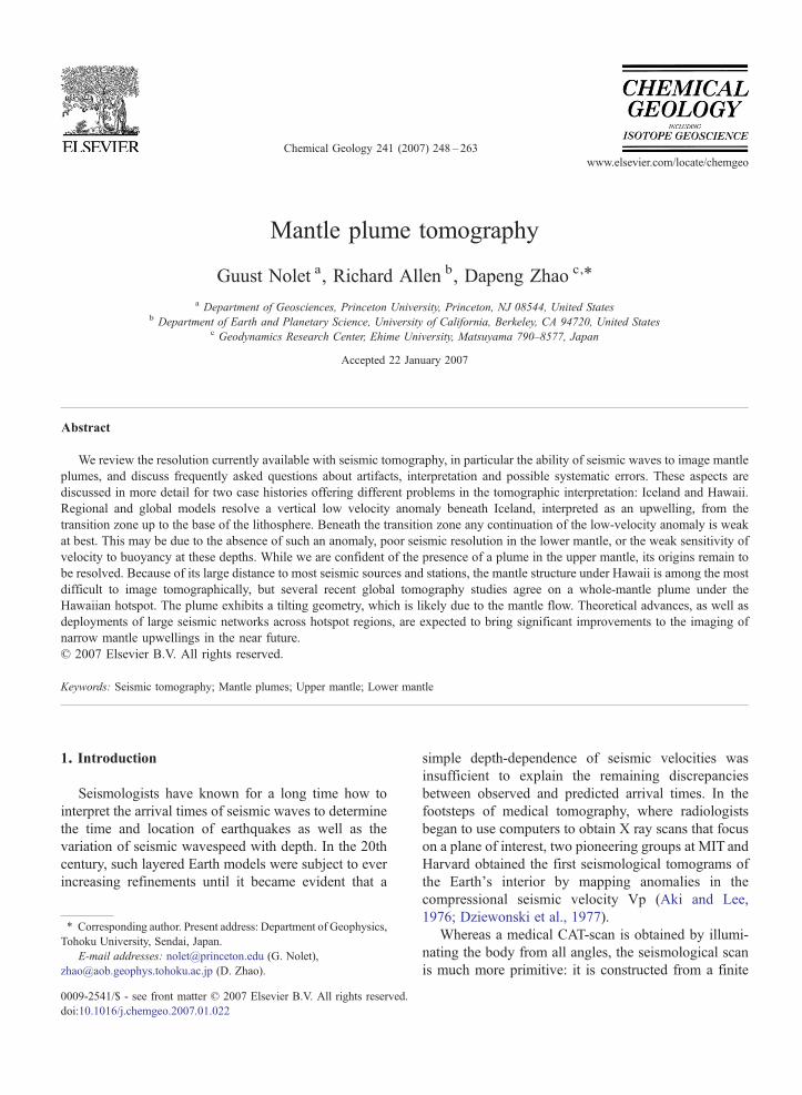
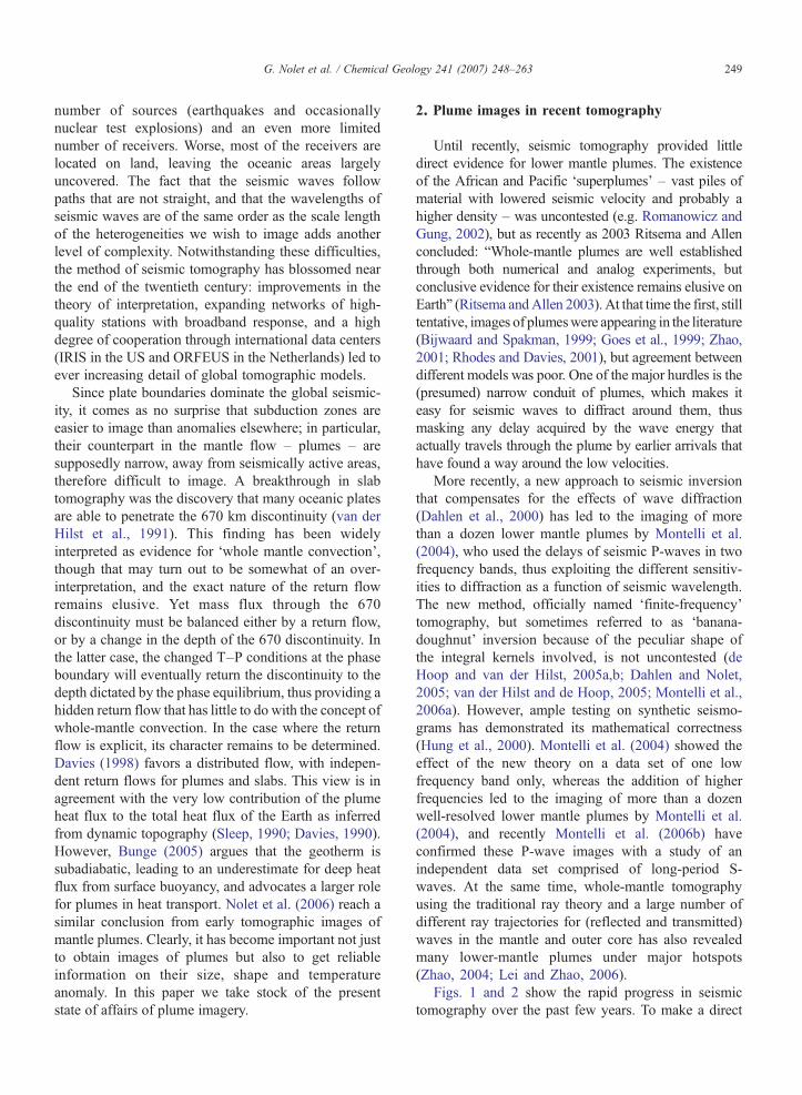
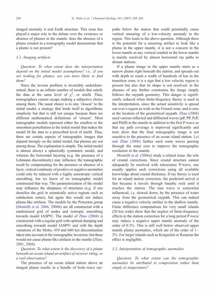
Figs. 1 and 2 show the rapid progress in seismictomography over the past few years. To make a direct


250 G. Nolet et al. / Chemical Geology 241 (2007) 248–263

comparison between anomalies in P and S velocitypossible (Fig. 1A, B and C, D respectively) the seismicvelocity has been translated into temperature using

Fig. 1. Four different tomographic images of the Tahiti plume, after translatin(C) PRI-S05 (Montelli et al., 2006b. (B) a P-wave model by Zhao (2004) and (temperature anomaly contours are in Kelvin.

estimates of the velocity-temperature derivative (Noletet al., 2006). Of the four models, PRI-P05 in Fig. 1A isthe best constrained image, using P, pP and PP delay time

g seismic velocity anomalies into temperature: (A) model PRI-P05 andD) model S20RTS from Ritsema et al., 1999). Depth is indicated in km,


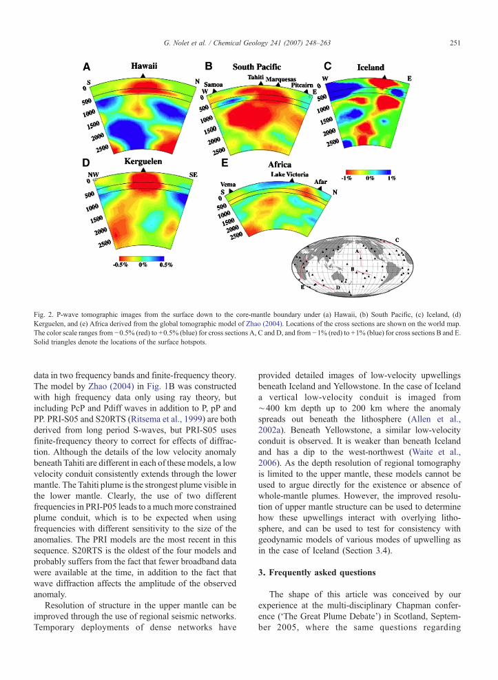
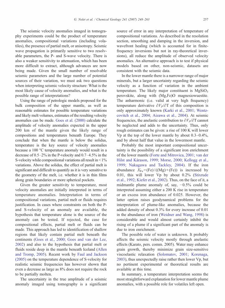
Fig. 2. P-wave tomographic images from the surface down to the core-mantle boundary under (a) Hawaii, (b) South Pacific, (c) Iceland, (d)Kerguelen, and (e) Africa derived from the global tomographic model of Zhao (2004). Locations of the cross sections are shown on the world map.The color scale ranges from −0.5% (red) to +0.5% (blue) for cross sections A, C and D, and from −1% (red) to +1% (blue) for cross sections B and E.Solid triangles denote the locations of the surface hotspots.


data in two frequency bands and finite-frequency theory.The model by Zhao (2004) in Fig. 1B was constructedwith high frequency data only using ray theory, butincluding PcP and Pdiff waves in addition to P, pP andPP. PRI-S05 and S20RTS (Ritsema et al., 1999) are bothderived from long period S-waves, but PRI-S05 usesfinite-frequency theory to correct for effects of diffrac-tion. Although the details of the low velocity anomalybeneath Tahiti are different in each of these models, a lowvelocity conduit consistently extends through the lowermantle. The Tahiti plume is the strongest plume visible inthe lower mantle. Clearly, the use of two differentfrequencies in PRI-P05 leads to amuchmore constrainedplume conduit, which is to be expected when usingfrequencies with different sensitivity to the size of theanomalies. The PRI models are the most recent in thissequence. S20RTS is the oldest of the four models andprobably suffers from the fact that fewer broadband datawere available at the time, in addition to the fact thatwave diffraction affects the amplitude of the observedanomaly.

Resolution of structure in the upper mantle can beimproved through the use of regional seismic networks.Temporary deployments of dense networks have

provided detailed images of low-velocity upwellingsbeneath Iceland and Yellowstone. In the case of Icelanda vertical low-velocity conduit is imaged from∼400 km depth up to 200 km where the anomalyspreads out beneath the lithosphere (Allen et al.,2002a). Beneath Yellowstone, a similar low-velocityconduit is observed. It is weaker than beneath Icelandand has a dip to the west-northwest (Waite et al.,2006). As the depth resolution of regional tomographyis limited to the upper mantle, these models cannot beused to argue directly for the existence or absence ofwhole-mantle plumes. However, the improved resolu-tion of upper mantle structure can be used to determinehow these upwellings interact with overlying litho-sphere, and can be used to test for consistency withgeodynamic models of various modes of upwelling asin the case of Iceland (Section 3.4).

3. Frequently asked questions

The shape of this article was conceived by ourexperience at the multi-disciplinary Chapman confer-ence (‘The Great Plume Debate’) in Scotland, Septem-ber 2005, where the same questions regarding


tomographic images of elusive objects such as plumeskept being asked. We followed up by inviting theconference participants to submit their lists of questionsby electronic mail. In this section we have grouped themost frequently asked questions into subsections.

3.1. Resolution of seismic tomography

Question: What is the spatial resolution of tomo-graphic images in the upper mantle?

The resolution of any specific tomographic image isdependent on the dataset and tomographic techniqueused, and can be determined using resolution tests,which are discussed later. However, some general rulesof thumb for resolution of different types of study areperhaps useful as a guide.

3.1.1. Surface wavesMany tomographic studies of the upper mantle use

surface waves. The horizontal travel paths of surfacewaves allow resolution of primarily S-velocity structurebeneath regions where there are no or few earthquakesand seismometers, e.g. beneath the oceans. Away fromdense seismic networks the horizontal resolution isusually determined by the density of crossing ray pathsand is therefore dependent on the specific geometry ofthe dataset. In this situation resolution tests – asdescribed later – can provide information on the sizeand geometry of structures that can be resolved for aparticular ray-path coverage. Even when a denseseismic network is available, typically on the con-tinents, the horizontal resolution is theoretically limitedby the width of the Fresnel Zone, wF, which isapproximately equal to

ffiffiffiffiffiffi

kLp

at its widest point halfway between the source and receiver. L is the pathlength and λ is the wavelength, equal to the product ofwave velocity and the period of the wave. Continent-scale models typically use periods of ∼100 s and pathlengths of ∼3000 km (e.g. van der Lee and Nolet, 1997;Debayle and Kennett, 2000; Simons et al., 2002) whichcorrespond to a wF of ∼1200 km. Regional scale ex-periments typically use higher frequencies and shorterpaths. In the recent Iceland HOTSPOT experimentsurface waves at periods of 30 to 10 s were used withpath lengths of 100–300 km (Allen et al., 2002a,b),reducing wF to 50–150 km.

While the higher frequencies improve the horizontalresolution, they also reduce the maximum depth that canbe resolved. Only the crust and uppermost mantle can beresolved with 30 to 10 s period waves. Surface waves ata given frequency are sensitive to a wide depth range,but the peak sensitivity of the dominant fundamental

mode is at a depth of approximately λ/3 for Rayleighwaves and λ/4 for Love waves. They have reasonablesensitivity to a depth of about twice the peak depth.When using 100 s surface waves, the peak sensitivity forRayleigh and Love waves is at depths of ∼150 and∼110 km and they can resolve structure to depths of∼300 and ∼220 km respectively. Resolution can beextended to greater depths using higher-mode surfacewaves, which requires more complex analysis but can bedone, e.g. by fitting the seismic waveforms in the timewindow following the arrival of the SS wave using asummation of either surface wave modes (Nolet, 1990),or coupled normal modes (Li and Romanowicz, 1995).Using higher mode surface waves, sensitivity can beextended to the transition zone but is still limited to theupper mantle. The depth resolution for surface waves isconsiderably better than the lateral resolution. Whensurface waves with a range of different frequencies areused, the depth resolution is typically tens of kilometers,meaning that a velocity anomaly at 50 km depth can bedistinguished from one at 100 km.

In summary, continent-scale surface wave studies canresolve lithospheric and asthenospheric structure to300–400 km depth with vertical resolution at the scaleof tens of kilometers and lateral resolution at the scale of∼1000 km. Resolution can be improved using denseregional networks and higher frequencies, but thishigher resolution is only obtainable for shallowerdepths.

3.1.2. Body wavesWhile surface waves have horizontal paths, body

waves through the upper mantle have predominantlyvertical paths. This means that body-wave constraintsare the natural complement to surface-wave datasets asthey can significantly enhance the lateral resolution(Ritsema et al., 1999; Allen et al., 2002a,b). Body-wavestudies also provide constraints on both P- and S-velocity structure but require stations above the studyregion. The Fresnel zone narrows down towards thereceiver, and high frequency body waves can, inprinciple, resolve horizontal variations adequately withresolution comparable to that of the station spacing oreven higher when both direct and reflected waves areused (e.g., Zhao et al., 2005). The vertical resolution ofall tomographic studies is dependent on the extent towhich the travel paths of the seismic energy (i.e. raypaths) cross each other. When using body-waves alone,the number of crossing paths is increased by threefactors: having a range of epicentral distances, a range ofback azimuths, and as large a number of stations over aswide an area as possible. The angle of the ray path to the


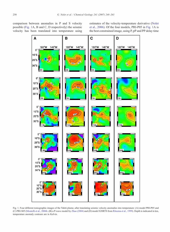
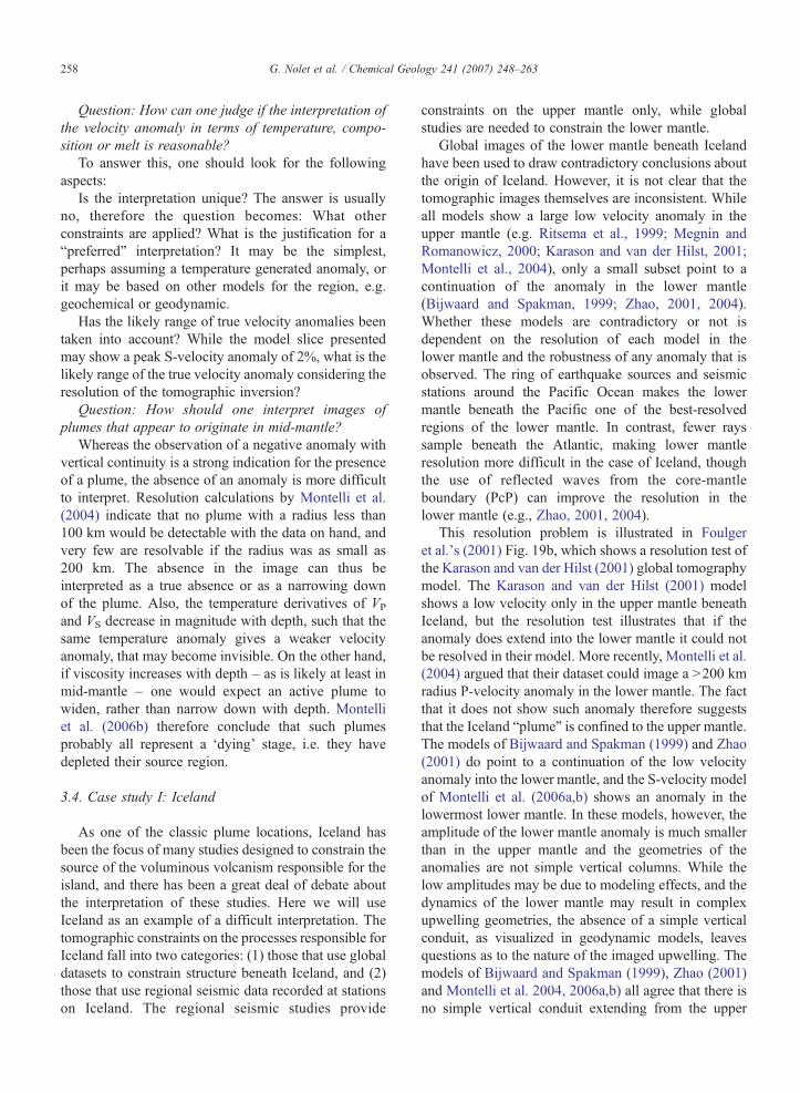
vertical is a function of the epicentral distance. Typicalteleseismic studies use P- and S-wave arrivals atepicentral distances of 30° to 90° as well as phasesthat travel through the Earth's core (i.e. PKP, PKIKPand SKS). In the upper mantle, P- and S-wave travel atangles between ∼25° and ∼45° to the vertical, whereasthe core phases are all within ∼20° of vertical. Themaximum depth that can be resolved is determined bythe aperture of the network being used. If straight, raypaths at 45° to the vertical from both ends of an arraywill cross at a depth of a/2 beneath the center of thearray where a is the network aperture. In the real earth,the bending of rays cause a slightly more complicateddepth dependence; for example, P-wave arriving at anepicentral distance of 36° cross at a depth equal to thearray span a. In practice, this is the maximum depth thatcan be adequately resolved. The use of finite frequencykernels (a.k.a. banana-doughnut kernels) does extendthe depth resolution due to the finite width of the kernels(e.g. Hung et al., 2004), but the larger volume of thekernels at these greater depths may also reduce thespatial resolution. Fig. 3 shows two resolution tests thatillustrate how the depth extent of resolution varies withthe network aperture.

Question: And what can we resolve in the lowermantle?

Surface waves do not reach into the lower mantle, butthe discrete normal modes of the Earth do, at the expenseof a further lengthening of horizontal wavelength(1000 km or more) and the resulting loss of horizontalresolution. The seismic wavelength poses a theoreticallimit to the resolution, in the sense that objects muchsmaller than the width of the Fresnel zone cannot berecovered even with finite-frequency tomography. Usefulresolution – certainly if we wish to image narrow objectslike mantle plumes or slab fragments – can thus only beobtained using bodywaves, possibly in addition to normalmode frequencies. It would thus pay to go to ever and everhigher frequency but teleseismic frequencies are limitedby anelastic attenuation. As a rule of thumb, the shortestwavelength, λ, for both P-wave and S-wave studies of thelower mantle is about 10 km. Teleseismic rays typi-cally have lengths between 5000 and 10,000 km, leadingto wF ≈200–300 km for the highest frequencies. Themajor limitation to body-wave resolution in the lowermantle is therefore the path coverage, which is still poor inmany regions of the lower mantle.

Question: What are the realistic limitations of thetechnique? Or, put another way, what can we expect inthe future?

Finite-frequency tomography has no difficulty cor-recting for the diffraction effects of objects about half

the Fresnel width (Hung et al., 2000), and so it seemsthe shortest wavelengths available could in principle beused to give details even of plume conduits. However,using short wavelengths in order to resolve narrowanomalies is not only a blessing, but also a curse: if theraypath ‘misses’ the plume it will not sense the anomaly.Especially in the Southern hemisphere, path coverage issparse and the larger width of a low-frequencywavepath pays off by providing sensitivity in regionsnot covered by the raypath as computed by Snell's law.Efforts are currently under way to re-measure traveltime delays in a range of frequency bands, thus fullyexploiting finite-frequency effects (Sigloch and Nolet,2006). Waveform inversions of the kind proposedtheoretically by Tromp et al. (2005) are a generalizationof the finite-frequency ideas, and should lead to evenbetter exploitation of the information in a seismogram.Such methods however are nonlinear, require massivecompute power, and have yet to show their practicalfeasibility.

In summary, therefore, the theoretically obtainableresolution is high (even better than 100 km) where theFresnel zone is narrow, i.e. in the upper mantle, or atdepth if raypath coverage is dense and finite-frequencytheory is used in the interpretation. If the geophysicalcommunity is able to launch a major effort to cover theoceans with seismic sensors, a resolution of about200 km should be feasible for the entire lower mantle.This, however, would involve investments comparableto those spent for the first human explorations at thesurface of the Moon. More realistically, a limitedincrease in coverage, coupled with advanced interpre-tation methods for waveforms or delays in differentfrequency bands, may eventually lead to a resolution ofthe order of 400 km in selected regions of the lowermantle. A theoretical limit is imposed by the minimumwavelength of seismic waves which leads to irrecover-able loss of signal for anomalies much smaller than theFresnel zone; in practice this means that anomaliesmuch smaller than about 200 km in the lowermostmantle – of the order of 100 km if finite-frequencytheory is used – can never be resolved with seismictomography.

Question: How does one estimate the actualresolution in a tomographic image?

Not all the fast and slow anomalies visible in atomographic image are reliable features, and theamplitude of an anomaly is usually less well constrainedthan its shape. Even a well-resolved tomographic imagecan be affected by the type of model parameterization(grid nodes, blocks, spherical harmonics), and thelimitations imposed by it, as well as by damping and

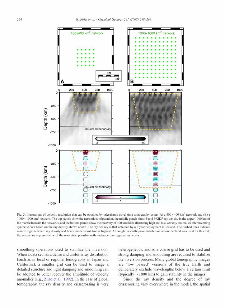
Fig. 3. Illustrations of velocity resolution that can be obtained by teleseismic travel time tomography using (A) a 400×400 km2 network and (B) a1000×1000 km2 network. The top panels show the network configuration, the middle panels show P and PKIKP ray density in the upper 1000 km ofthe mantle beneath the networks, and the bottom panels show the recovery of 100 km thick alternating high and low velocity anomalies after invertingsynthetic data based on the ray density shown above. The ray density is that obtained by a 2 year deployment in Iceland. The dashed lines indicatemantle regions where ray density and hence model resolution is highest. Although the earthquake distribution around Iceland was used for this test,the results are representative of the resolution possible with wide-aperture regional networks.


smoothing operations used to stabilize the inversion.When a data set has a dense and uniform ray distribution(such as in local or regional tomography in Japan andCalifornia), a smaller grid can be used to image adetailed structure and light damping and smoothing canbe adopted to better recover the amplitude of velocityanomalies (e.g., Zhao et al., 1992). In the case of globaltomography, the ray density and crisscrossing is very

heterogeneous, and so a coarse grid has to be used andstrong damping and smoothing are required to stabilizethe inversion process. Many global tomographic imagesare ‘low passed’ versions of the true Earth anddeliberately exclude wavelengths below a certain limit(typically ∼1000 km) to gain stability in the images.

Since the ray density and the degree of raycrisscrossing vary everywhere in the model, the spatial


resolution and reliability of the tomographic imagechange from place to place. To evaluate whether afeature is reliable or not, it is necessary to perform aspecific resolution analysis for that feature. Tomogra-phers use “sensitivity tests” to evaluate the reliability ofa feature of interest. This is done as follows: first, asynthetic input model is constructed that includes thefeature to be examined (either a slab or a plume) withits geometry similar to that appearing in a realtomographic image. Secondly, synthetic data (e.g.travel times) are calculated for the synthetic inputmodel. The numbers of stations, earthquakes and raysare the same as those in the real data set, and the samecomputational algorithms are used. To simulate theobservation errors in the real data, (random) noise isalso added to the calculated synthetic data. Thirdly, thesynthetic data are inverted using the same inversionalgorithm as that for the real data. Finally, the inversionresult is compared with the input synthetic model to seewhether and how well the assumed feature is recovered.If the general geometry of the feature is reconstructed,then it is considered to be “reliable”, though theamplitude of the velocity anomaly is generally not fullyrecovered because of the damping and smoothing. Ifthis is repeated using different realizations of therandom noise, we also obtain an impression of theinfluence of data errors. Examples of such synthetictests can be found in Zhao (2001, 2004) and Montelliet al. (2004, 2006b).

Tomographers also use so-called “checkerboardresolution tests” (CRT) to evaluate the resolution of atomographic image. The CRT is a generalized form ofthe resolution test. The input model resembles acheckerboard with alternating positive and negativeanomalies. One conducts the checkerboard tests withdifferent grid spacings (or block sizes). The CRT isuseful to view the reliability of the entire modelingspace, but it is not sufficient to judge whether a specialfeature (like plume or slab) is resolved or not. Generally,tomographers conduct both types of synthetic tests toexamine the overall resolution scale of the entire modelas well as the reliability of some specific features such asa slab or a plume.

Question: How does one judge if an observedtomographic anomaly is resolved?

This is often the most difficult question for the non-seismologist to answer if one is using results from apublished tomographic paper. Here are some aspects towatch out for:

What type of data is being used in the inversion? Ifsurface waves are used, the maximum depth ofresolution is about 2λ/3 for Rayleigh waves, 2λ/4 for

Love waves, deeper if higher modes are used. If body-waves are being used, to what extent are the ray-pathscrossing in the region of the anomaly? Both azimuthalvariation and epicentral distance variations result incrossing paths along with the use of different phases, i.e.mantle and core phases. Beware of anomalies at theedge of the resolved region as they may be structuressmeared into the model.

Is smearing a problem? Does the velocity anomalyhave a structure similar in geometry to the sensitivity ofthe dataset being used? Examples include elongatedanomalies along body-wave ray paths or horizontalstripes along surface wave paths.

Are there resolution tests? Do they support theassertion that the observed anomaly is real? Resolutiontests, using synthetic velocity anomalies that are bothsimilar and different in geometry to the observedanomaly, are important. Spike, blob or checkerboardtests indicate the scale of anomaly that can be resolvedand also illustrate the extent of smearing. Tests using ananomaly of similar geometry to the observed anomalycan indicate the effects of smoothing and damping.Beware of resolution tests that only use a syntheticmodel with the same geometry as the observed. If anobserved anomaly is the result of smearing true Earthstructure along ray paths, the reconstructed anomaly willhave extra smearing in the resolution test but this is notalways clearly recognizable.

Question: Does the absence of an anomaly in atomographic model imply that there is no such velocitystructure in the Earth?

Again, we feel this is best answered by providing achecklist:

What is the model resolution? To argue that a struc-ture is absent requires demonstration that it would beresolved if it existed. A resolution test demonstratingthe resolvability of the allegedly absent anomaly isnecessary.

Is the seismic wavefield observed at the surfacesensitive to the allegedly absent structure? The rules ofthumb regarding the wavelengths and Fresnel zones thatwe discussed earlier may give a useful first orderanswer. More exact answers require a test that goesbeyond the computational algorithm being used (e.g.shortcomings of ray theory will not be visible in aresolution test using ray theory). A test using fullwaveform propagation, such as the spectral elementmethod (SEM) is the best way to answer this question.

Unfortunately, there is no simple test to answer thequestion. Accordingly, it is much more difficult to arguethat an absent anomaly means there is no velocitystructure in the mantle, than to demonstrate that an


imaged anomaly is real Earth structure. This issue hasplayed a major role in the debate over the existence orabsence of plumes in the mantle: does the absence of aplume conduit in a tomography model demonstrate thata plume is not present?

3.2. Imaging artifacts

Question: To what extent does the interpretationdepend on the initial model assumptions? i.e., if youare looking for plumes, are you more likely to findthem?

Since the inverse problem is invariably underdeter-mined, there is an infinite number of models that satisfythe data at the same level of χ2, or misfit. Thus,tomographers cannot escape making a subjective choiceamong them. The usual choice is to stay ‘closest’ to theinitial model, a strategy that lends itself to algorithmicsimplicity but that is still not unique because there aredifferent mathematical definitions of ‘closest’. Mosttomographic models represent either the smallest or thesmoothest perturbation to the initial model that makes themodel fit the data to a prescribed level of misfit. Thus,there are certain aspects of tomographic images thatdepend strongly on the initial model, but plumes are notamong those. The explanation is simple. The initial modelis almost always a spherically symmetric model, andwhereas the horizontal layering (e.g. the presence of aLehmann discontinuity) may influence the tomographicresult by compensating for the presence or absence of alayer, vertical continuity of positive or negative anomaliescould only be induced with a highly anisotropic verticalsmoothing, but we know of no tomographic modelconstructed that way. The parameterization of the modelmay influence the sharpness of structures (e.g. if onedensifies the grid in seismically active regions such assubduction zones), but again this would not induceplume-like artifacts. The models by the Princeton group(Montelli et al. 2004, 2006b) are all constructed with arandomized grid of nodes and isotropic smoothingtowards model IASP91. The model of Zhao (2004) isconstructed with a regular grid with optimal damping andsmoothing towards model IASP91 and with the depthvariations of the Moho, 410 and 660 km discontinuitiestaken into account in the tomographic inversion, but thesewould not cause plume-like artifacts in the mantle (Zhao,2001, 2004).

Question: To what extent is the discovery of a plumebeneath an ocean island an artifact of receiver siting, ora real observation?

The presence of an ocean island station above animaged plume results in a bundle of body-wave ray-

paths below the station that could potentially causevertical smearing of a low-velocity anomaly in theregion. This leads to the above question. Although thereis the potential for a smearing artifact to look like aplume in the upper mantle, it is not a concern in thelower mantle as any vertical conduit in the lower mantleis mainly resolved by almost horizontal ray paths todistant stations.

If a plume image in the upper mantle starts as anarrow plume right beneath the station, and spreads outwith depth to reach a width of hundreds of km in thetransition zone, it is a sign that a low velocity region ispresent but also that its shape is not resolved: in theabsence of any further constraints the image simplyfollows the raypath geometry. This danger is signifi-cantly reduced when finite-frequency theory is used inthe interpretation, since the actual sensitivity is spreadout over a region as wide as the Fresnel zone, and is zeroat the location of the geometrical raypath. Zhao (2004)used various reflected and diffracted waves (pP, PP, PcP,and Pdiff) in the mantle in addition to the first P-wave sothat ray path coverage is improved significantly andtests show that the final tomographic image is notsensitive to the presence of an ocean island station. Leiand Zhao (2006) further used some waves passingthrough the outer core to improve the tomographicresolution in the mantle.

Montelli et al. (2006a) study a related issue: the roleof crustal corrections. Since crustal structure cannotadequately be resolved with teleseismic P-wave, oneusually applies such corrections using all availableknowledge about crustal thickness. If ray theory is usedfor an island station correction, the predicted arrival isfast because it travels through basaltic rock until itreaches the station. The true wave is somewhatinfluenced, i.e. slowed down, by the presence of wateraway from the geometrical raypath. This can indeedcause a negative velocity artifact in the shallow mantle.Finite difference computations for very small islands(20 km wide) show that the neglect of finite-frequencyeffects in the station correction for a long period P-wavemay induce a negative upper mantle anomaly of theorder of 0.3%. This is still well below observed uppermantle plume anomalies, which are of the order of 1–2%. For larger islands such as Kerguelen or Reunion theeffect is negligible.

3.3. Interpretation of tomographic anomalies

Question: To what extent can the tomographicanomalies be attributed to composition rather thansimply to temperature?


The seismic velocity anomalies imaged in tomogra-phy experiments could be the product of temperatureanomalies, compositional variations (including vola-tiles), the presence of partial melt, or anisotropy. Seismicwave propagation is primarily sensitive to two resolv-able parameters, the P- and S-wave velocity. There isalso a weaker sensitivity to attenuation, which has beenmore difficult to extract, although advances are nowbeing made. Given the small number of resolvableseismic parameters and the large number of potentialsources of their variation, we must ask two questionswhen interpreting seismic velocity structure: What is themost likely cause of velocity anomalies, and what is thepossible range of interpretations?

Using the range of petrologic models proposed for thebulk composition of the upper mantle, as well asreasonable estimates for possible temperature variationsand likelymelt volumes, estimates of the resulting velocityanomalies can be made. Goes et al. (2000) calculate theamplitude of velocity anomalies expected in the upper200 km of the mantle given the likely range ofcompositions and temperatures beneath Europe. Theyconclude that when the mantle is below the solidus,temperature is the key source of velocity anomaliesbecause a 100 °C temperature anomaly would result in adecrease of 0.5–2% in the P-velocity and 0.7–4.5% in theS-velocitywhile compositional variations all result inb1%variations. Above the solidus, the effect of partial melt issignificant and difficult to quantify as it is very sensitive tothe geometry of the melt, i.e. whether it is in thin filmsalong grain boundaries or more spherical pockets.

Given the greater sensitivity to temperature, mostvelocity anomalies are initially interpreted in terms oftemperature anomalies. Interpretation in terms ofcompositional variations, partial melt or fluids requiresjustification. In cases where constraints on both the P-and S-velocity of an anomaly are available, thehypothesis that temperature alone is the source of theanomaly can be tested. If rejected, the case forcompositional effects, partial melt or fluids can bemade. This approach has led to identification of shallowregions that likely contain partial melt beneath thecontinents (Goes et al., 2000; Goes and van der Lee,2002) and also to the hypothesis that partial melt orfluids reside deep in the mantle beneath Iceland (Allenand Tromp, 2005). Recent work by Faul and Jackson(2005) on the temperature dependence of S-velocity forrealistic seismic frequencies has however shown thateven a decrease as large as 8% does not require the rockto be partially molten.

The uncertainty in the true amplitude of a seismicanomaly imaged using tomography is a significant

source of error in any interpretation of temperature ofcompositional variations. As described in the resolutionsection, smoothing and damping in the inversion, andwavefront healing (which is accounted for in finite-frequency inversions but not in ray-theoretical inver-sions), all reduce the amplitude of observed velocityanomalies. An alternative approach is to test if physicalmodels based on other, non-seismic, datasets areconsistent with the seismic data.

In the lower mantle there is a narrower range of majorminerals, but a larger uncertainty regarding the seismicvelocity as a function of variation in the ambienttemperature. The likely major constituent is MgSiO3

perovskite, along with (Mg,Fe)O magnesiowuestite.The anharmonic (i.e. valid at very high frequency)temperature derivative ∂VP/∂T of this composition isonly approximately known (Karki et al., 2001; Wentz-covitch et al., 2004; Aizawa et al., 2004). At seismicfrequencies, the anelastic contribution to ∂VP/∂T cannotbe neglected and adds to the uncertainty. Thus, onlyrough estimates can be given: a rise of 100 K will lowerVp at the top of the lower mantle by about 0.3–0.4%,and by about half that value in the lowermost mantle.

Probably the most important compositional uncer-tainty is the possibility of a significant iron enrichmentof the lower mantle (Forte and Mitrovica, 2001; van derHilst and Kárason, 1999; Morse, 2000; Kellogg et al.,1999; Nakagawa and Tackley, 2004). If the ironabundance XFe= (Fe) / ((Mg)+ (Fe)) is increased by0.01, this will lower Vp by about 0.2% (Stixrudeet al., 1992; Kiefer et al., 2002). Thus, on the face of it, amidmantle plume anomaly of, say, −0.5% could beinterpreted assuming either a 200 K rise in temperatureor an excess iron abundance of 0.025. However, thelatter option raises geodynamical problems for theinterpretation of plume-like anomalies, because theadded density of about 0.3% for every increase of 0.01in the abundance of iron (Weidner and Wang, 1998) isconsiderable and would almost certainly inhibit therising of a plume if a significant part of the anomaly isdue to iron enrichment.

The possible role of water is unknown. It probablyaffects the seismic velocity mostly through anelasticeffects (Karato, pers. comm. 2005). Water may enhancegrain growth, thereby minimize grain size-sensitiveviscoelastic relaxation (Solomatov, 2001; Korenaga,2003), thus unexpectedly raise rather then lower Vp, butno pertinent experimental or theoretical results areavailable at this time.

In summary, a temperature interpretation seems themost straightforward explanation for lowermantle plumeanomalies, with a possible role for volatiles left open.


Question: How can one judge if the interpretation ofthe velocity anomaly in terms of temperature, compo-sition or melt is reasonable?

To answer this, one should look for the followingaspects:

Is the interpretation unique? The answer is usuallyno, therefore the question becomes: What otherconstraints are applied? What is the justification for a“preferred” interpretation? It may be the simplest,perhaps assuming a temperature generated anomaly, orit may be based on other models for the region, e.g.geochemical or geodynamic.

Has the likely range of true velocity anomalies beentaken into account? While the model slice presentedmay show a peak S-velocity anomaly of 2%, what is thelikely range of the true velocity anomaly considering theresolution of the tomographic inversion?

Question: How should one interpret images ofplumes that appear to originate in mid-mantle?

Whereas the observation of a negative anomaly withvertical continuity is a strong indication for the presenceof a plume, the absence of an anomaly is more difficultto interpret. Resolution calculations by Montelli et al.(2004) indicate that no plume with a radius less than100 km would be detectable with the data on hand, andvery few are resolvable if the radius was as small as200 km. The absence in the image can thus beinterpreted as a true absence or as a narrowing downof the plume. Also, the temperature derivatives of VP

and VS decrease in magnitude with depth, such that thesame temperature anomaly gives a weaker velocityanomaly, that may become invisible. On the other hand,if viscosity increases with depth – as is likely at least inmid-mantle – one would expect an active plume towiden, rather than narrow down with depth. Montelliet al. (2006b) therefore conclude that such plumesprobably all represent a ‘dying’ stage, i.e. they havedepleted their source region.

3.4. Case study I: Iceland

As one of the classic plume locations, Iceland hasbeen the focus of many studies designed to constrain thesource of the voluminous volcanism responsible for theisland, and there has been a great deal of debate aboutthe interpretation of these studies. Here we will useIceland as an example of a difficult interpretation. Thetomographic constraints on the processes responsible forIceland fall into two categories: (1) those that use globaldatasets to constrain structure beneath Iceland, and (2)those that use regional seismic data recorded at stationson Iceland. The regional seismic studies provide

constraints on the upper mantle only, while globalstudies are needed to constrain the lower mantle.

Global images of the lower mantle beneath Icelandhave been used to draw contradictory conclusions aboutthe origin of Iceland. However, it is not clear that thetomographic images themselves are inconsistent. Whileall models show a large low velocity anomaly in theupper mantle (e.g. Ritsema et al., 1999; Megnin andRomanowicz, 2000; Karason and van der Hilst, 2001;Montelli et al., 2004), only a small subset point to acontinuation of the anomaly in the lower mantle(Bijwaard and Spakman, 1999; Zhao, 2001, 2004).Whether these models are contradictory or not isdependent on the resolution of each model in thelower mantle and the robustness of any anomaly that isobserved. The ring of earthquake sources and seismicstations around the Pacific Ocean makes the lowermantle beneath the Pacific one of the best-resolvedregions of the lower mantle. In contrast, fewer rayssample beneath the Atlantic, making lower mantleresolution more difficult in the case of Iceland, thoughthe use of reflected waves from the core-mantleboundary (PcP) can improve the resolution in thelower mantle (e.g., Zhao, 2001, 2004).

This resolution problem is illustrated in Foulgeret al.'s (2001) Fig. 19b, which shows a resolution test ofthe Karason and van der Hilst (2001) global tomographymodel. The Karason and van der Hilst (2001) modelshows a low velocity only in the upper mantle beneathIceland, but the resolution test illustrates that if theanomaly does extend into the lower mantle it could notbe resolved in their model. More recently, Montelli et al.(2004) argued that their dataset could image a N200 kmradius P-velocity anomaly in the lower mantle. The factthat it does not show such anomaly therefore suggeststhat the Iceland “plume” is confined to the upper mantle.The models of Bijwaard and Spakman (1999) and Zhao(2001) do point to a continuation of the low velocityanomaly into the lower mantle, and the S-velocity modelof Montelli et al. (2006a,b) shows an anomaly in thelowermost lower mantle. In these models, however, theamplitude of the lower mantle anomaly is much smallerthan in the upper mantle and the geometries of theanomalies are not simple vertical columns. While thelow amplitudes may be due to modeling effects, and thedynamics of the lower mantle may result in complexupwelling geometries, the absence of a simple verticalconduit, as visualized in geodynamic models, leavesquestions as to the nature of the imaged upwelling. Themodels of Bijwaard and Spakman (1999), Zhao (2001)and Montelli et al. 2004, 2006a,b) all agree that there isno simple vertical conduit extending from the upper




mantle down through the lower mantle beneath Iceland.Therefore, the nature of any lower mantle upwellingbeneath Iceland, should it exist, remains elusive.

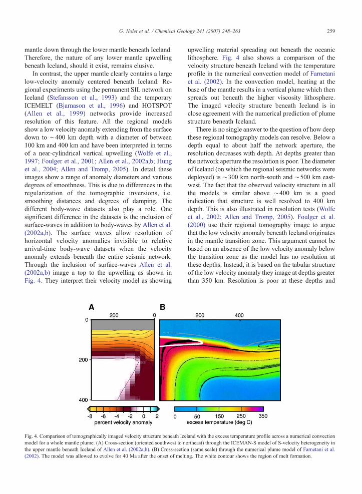
In contrast, the upper mantle clearly contains a largelow-velocity anomaly centered beneath Iceland. Re-gional experiments using the permanent SIL network onIceland (Stefansson et al., 1993) and the temporaryICEMELT (Bjarnason et al., 1996) and HOTSPOT(Allen et al., 1999) networks provide increasedresolution of this feature. All the regional modelsshow a low velocity anomaly extending from the surfacedown to ∼400 km depth with a diameter of between100 km and 400 km and have been interpreted in termsof a near-cylindrical vertical upwelling (Wolfe et al.,1997; Foulger et al., 2001; Allen et al., 2002a,b; Hunget al., 2004; Allen and Tromp, 2005). In detail theseimages show a range of anomaly diameters and variousdegrees of smoothness. This is due to differences in theregularization of the tomographic inversions, i.e.smoothing distances and degrees of damping. Thedifferent body-wave datasets also play a role. Onesignificant difference in the datasets is the inclusion ofsurface-waves in addition to body-waves by Allen et al.(2002a,b). The surface waves allow resolution ofhorizontal velocity anomalies invisible to relativearrival-time body-wave datasets when the velocityanomaly extends beneath the entire seismic network.Through the inclusion of surface-waves Allen et al.(2002a,b) image a top to the upwelling as shown inFig. 4. They interpret their velocity model as showing

Fig. 4. Comparison of tomographically imaged velocity structure beneath Icemodel for a whole mantle plume. (A) Cross-section (oriented southwest to nothe upper mantle beneath Iceland of Allen et al. (2002a,b). (B) Cross-sectio(2002). The model was allowed to evolve for 40 Ma after the onset of melti

upwelling material spreading out beneath the oceaniclithosphere. Fig. 4 also shows a comparison of thevelocity structure beneath Iceland with the temperatureprofile in the numerical convection model of Farnetaniet al. (2002). In the convection model, heating at thebase of the mantle results in a vertical plume which thenspreads out beneath the higher viscosity lithosphere.The imaged velocity structure beneath Iceland is inclose agreement with the numerical prediction of plumestructure beneath Iceland.

There is no single answer to the question of how deepthese regional tomography models can resolve. Below adepth equal to about half the network aperture, theresolution decreases with depth. At depths greater thanthe network aperture the resolution is poor. The diameterof Iceland (on which the regional seismic networks weredeployed) is ∼300 km north-south and ∼500 km east-west. The fact that the observed velocity structure in allthe models is similar above ∼400 km is a goodindication that structure is well resolved to 400 kmdepth. This is also illustrated in resolution tests (Wolfeet al., 2002; Allen and Tromp, 2005). Foulger et al.(2000) use their regional tomography image to arguethat the low velocity anomaly beneath Iceland originatesin the mantle transition zone. This argument cannot bebased on an absence of the low velocity anomaly belowthe transition zone as the model has no resolution atthese depths. Instead, it is based on the tabular structureof the low velocity anomaly they image at depths greaterthan 350 km. Resolution is poor at these depths and

land with the excess temperature profile across a numerical convectionrtheast) through the ICEMAN-S model of S-velocity heterogeneity inn (same scale) through the numerical plume model of Farnetani et al.ng. The white contour shows the region of melt formation.


other regional models using larger datasets have failedto image a similar structure so the observation remainsunconfirmed.

The maximum depth resolution of the regionalIceland datasets has recently been extended to the baseof the transition zone through improvement in thetomographic technique to account for finite-frequencyeffects. Application of the broad banana-doughnutkernels more accurately represents the width of theregion to which a traveltime measurement is sensitive.This improved representation of the sensitivity ofseismic arrivals allows information about deeperstructure to be extracted in the tomographic inversion.Using this approach Hung et al. (2004) show that thelow velocity extends to the base of the transition zone.Even with these improved techniques, however, it is stillnot possible to use the regional datasets to determine ifthe conduit extends through into the lower mantle.

Massive computers and advances in numericaltechniques now make it possible to propagate seismicwavefields through three dimensional velocity struc-tures to forward calculate synthetic waveforms whichcan be compared to observed data. These forwardcalculations, such as the Spectral Element Method(SEM) (Komatitsch and Tromp, 2002a,b), do not makethe simplifying assumptions used in tomographictechniques and therefore provide an opportunity to testtomographic models to see if they reproduce theobservations from which they were generated. TheICEMAN models for the Icelandic upper mantle (Allenet al., 2002a,b), generated using ray theory, were testedusing the SEM (Allen and Tromp, 2005). The tests showthat the ICEMAN models represent an end-member in arange of velocity structures that satisfy the seismicobservations. As expected, the tomographic techniquebroadened the vertical conduit and reduced the ampli-tude of the seismic anomaly. By testing differentdiameter upwellings the allowable range was deter-mined to be from ∼150 km up to 200 km in diameter.The upper limit is equal to that observed in the raytheoretical models, but the true amplitude of the seismicvelocity is likely twice the ray-theoretical value. Theminimum diameter of the conduit is constrained by thefact that a narrower conduit would not be observable atthe surface. Wavefront healing effects would erodedelays in the seismic wavefront as it approached thesurface, making the traveltime delays significantly lessthan those observed. Note that finite frequency inver-sions are less sensitive to image broadening, at least ifthey use a range of frequencies to exploit the sensitivityof wavefront healing to the size of the anomaly withrespect to the seismic wavelength.

To summarize, while tomographic images of themantle beneath Iceland have led to extensive debate, thevarious images are mostly consistent. There is a lowvelocity anomaly that extends through the upper mantle,which is widely interpreted as a buoyant upwelling thatspreads out beneath the oceanic lithosphere. Thestructure of this imaged upper mantle plume isconsistent with geodynamic models for whole mantleplumes. Whether this anomaly extends into the lowermantle is a continuing focus of research. In order tofinally answer this question we need improved datacoverage which is only obtainable using ocean bottomseismographs around Iceland.

3.5. Case study II: Hawaii

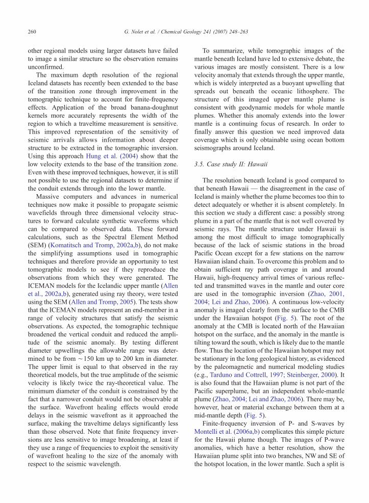
The resolution beneath Iceland is good compared tothat beneath Hawaii — the disagreement in the case ofIceland is mainly whether the plume becomes too thin todetect adequately or whether it is absent completely. Inthis section we study a different case: a possibly strongplume in a part of the mantle that is not well covered byseismic rays. The mantle structure under Hawaii isamong the most difficult to image tomographicallybecause of the lack of seismic stations in the broadPacific Ocean except for a few stations on the narrowHawaiian island chain. To overcome this problem and toobtain sufficient ray path coverage in and aroundHawaii, high-frequency arrival times of various reflec-ted and transmitted waves in the mantle and outer coreare used in the tomographic inversion (Zhao, 2001,2004; Lei and Zhao, 2006). A continuous low-velocityanomaly is imaged clearly from the surface to the CMBunder the Hawaiian hotspot (Fig. 5). The root of theanomaly at the CMB is located north of the Hawaiianhotspot on the surface, and the anomaly in the mantle istilting toward the south, which is likely due to the mantleflow. Thus the location of the Hawaiian hotspot may notbe stationary in the long geological history, as evidencedby the paleomagnetic and numerical modeling studies(e.g., Tarduno and Cottrell, 1997; Steinberger, 2000). Itis also found that the Hawaiian plume is not part of thePacific superplume, but an independent whole-mantleplume (Zhao, 2004; Lei and Zhao, 2006). There may be,however, heat or material exchange between them at amid-mantle depth (Fig. 5).

Finite-frequency inversion of P- and S-waves byMontelli et al. (2006a,b) complicates this simple picturefor the Hawaii plume though. The images of P-waveanomalies, which have a better resolution, show theHawaiian plume split into two branches, NW and SE ofthe hotspot location, in the lower mantle. Such a split is

Fig. 5. A north-south vertical cross section of P-wave tomography passing through Hawaii and South Pacific (Lei and Zhao, 2006). Location of thecross section is shown on the insert map. The color scale ranges from −1% (red) to +1% (blue). Solid triangles denote the locations of the surfacehotspots.


confirmed in the S-wave anomalies near 1000 km depth,but the S wave image disappears below 2000 km depth.

4. Conclusions

Every geophysical inverse problem is underdeter-mined, and requires a certain amount of subjectivejudgement from the interpreter to choose the preferredimage among many options. Progress is measured bythe ever increasing detail that shows up consistentlyamong those options. Very recently, plumes haveentered that realm. Though the images are still blurredand details are not the same among different efforts,there is no doubt that plumes exist in the lower mantle.

This article was written at a time that the technique oftomographic imaging is undergoing important changes.The GSN, a global network of digital, broadbandseismic stations, has only recently been completed tofull strength and the number of similar stations in othernetworks is still increasing. The broadband character ofthese data allows tomographers to mine the frequencydependence of seismic delays, which is a direct functionof the size of anomalies with respect to the width of theFresnel zone. The first plume images constructed withthe theory of finite-frequency tomography used only ahaphazard combination of two frequency bands, and islikely to be improved upon in the years to come.Increasing data coverage is also to be expected fromtemporary deployments both on land and in the oceans.For example, the USArray project is expected to bring ina wealth of data on the deep structure of the mantle

beneath Yellowstone. By all signs, seismic tomographyis entering a Golden Age.

Acknowledgements

We thank Geoffrey Davies, Ian Jackson and IanCarmichael for their constructive reviews of this paper.GN acknowledges support for tomographic researchfrom the NSF (EAR 0309298). NSF also providedsupport for RA's contribution (EAR 0539987). DZ issupported by grants (B-11440134, A-17204037) fromthe Japanese Ministry of Education and Science.

References

Aizawa, Y., Yoneda, A., Katsura, T., Ito, E., Saito, T., Suzuki, I., 2004.Temperature derivatives of elastic moduli of MgSiO3 perovskite.Geophys. Res. Lett. 31, L01602.

Aki, K., Lee, H., 1976. Determination of three-dimensional anomaliesunder a seismic array using first p arrival times from localearthquakes: 1. a homogeneous initial model. J. Geophys. Res. 81,4381–4399.

Allen, R.M., Tromp, J., 2005. Resolution of regional seismicmodels: squeezing the Iceland anomaly. Geophys. J. Int. 161,373–386.

Allen, R.M., Nolet, G., Morgan, W.J., Vogfjord, K., Bergsson, B.H.,Erlendsson, P., Foulger, G.R., Jakobsdottir, S., Julian, B.R.,Pritchard, M., Ragnarsson, S., Stefansson, R., 1999. The thin hotplume beneath Iceland. Geophys. J. Int. 137, 51–63.

Allen, R.M., Nolet, G., Morgan, W.J., Vogfjord, K., Bergsson, B.H.,Erlendsson, P., Foulger, G.R., Jakobsdottir, S., Julian, B.R.,Pritchard, M., Ragnarsson, S., Stefansson, R., 2002a. Imaging themantle beneath Iceland using integrated seismological techniques.J. Geophys. Res. 107, 2325. doi:10.1019/2001JB000595.



Allen, R.M., Nolet, G.,Morgan,W.J., Vogfjord, K.,Nettles,M., Ekstrom,G., Bergsson, B.H., Erlendsson, P., Foulger, G.R., Jakobsdottir, S.,Julian, B.R., Pritchard, M., Ragnarsson, S., Stefansson, R., 2002b.Plume driven plumbing and crustal formation in Iceland. J. Geophys.Res. 107, 2163. doi:10.1029/2001JB000584.

Bijwaard, H., Spakman, W., 1999. Tomographic evidence for a narrowwhole mantle plume below Iceland. Earth Planet. Sci. Lett. 166,121–126.

Bjarnason, I.-T., Wolfe, C.-J., Solomon, S.-C., Gudmundson, G., 1996.Initial results from the ICEMELT experiment: Body-wave delaytimes and shear-wave splitting across Iceland. Geophys. Res. Lett.23, 459–462.

Bunge, H., 2005. Low plume excess temperature and high core heatflux inferred from non-adiabatic geotherms in internally heatedmantle circulation models. Phys. Earth Planet. Inter. 153, 3–10.

Dahlen, F.A., Nolet, G., 2005. Comment on the paper on sensitivitykernels for wave equation transmission tomography by de Hoopand van der Hilst. Geophys. J. Int. 163, 949–951.

Dahlen, F.A., Hung, S.-H., Nolet, G., 2000. Frechet kernels for finite-frequency traveltimes— I. Theory. Geophys. J. Int. 141, 157–174.

Davies, G., 1990. Ocean bathymetry and mantle convection,1, large-scale flow and hotspots. J. Geophys. Res. 93, 10467–10480.

Davies, G., 1998. Topography: a robust constraint on mantle fluxes.Chem. Geol. 145, 479–489.

de Hoop, M., van der Hilst, R., 2005a. On sensitivity kernels for waveequation transmission tomography. Geophys. J. Int. 160, 621–633.

de Hoop, M., van der Hilst, R., 2005b. Reply to a comment by F.A.Dahlen and G. Nolet on: On sensitivity kernels for wave equationtomography. Geophys. J. Int. 163, 952–955.

Debayle, E., Kennett, B.L.N., 2000. Anisotropy in the Australasianupper mantle from Love and Rayleigh waveform inversion. EarthPlanet. Sci. Lett. 184, 339–351.

Dziewonski, A., Hager, B., O'Connell, R., 1977. Large-scaleheterogeneities in the lower mantle. J. Geophys. Res. 82, 239–255.

Farnetani, C.G., Lagras, B., Tackley, P.J., 2002. Mixing anddeformations in mantle plumes. Earth Planet. Sci. Lett. 196, 1–15.

Faul, U.H., Jackson, I., 2005. The seismological signature oftemperature and grain size variations in the upper mantle. EarthPlanet. Sci. Lett. 234, 119–134.

Forte, A., Mitrovica, J., 2001. Deep mantle high-viscosity flow andthermochemical structure inferred from seismic and geodynamicdata. Nature 410, 1049–1056.

Foulger, G.R., Pritchard, M.J., Julian, B.R., Evans, J.R., Allen, R.M.,Nolet, G., Morgan, W.J., Bergsson, B.H., Erlendsson, P.,Jakobsdottir, S., Ragnarsson, S., Stefansson, R., Vogfjord, K.,2000. The seismic anomaly beneath Iceland extends down to themantle transition zone and no deeper. Geophys. J. Int. 142, F1–F5.

Foulger, G.R., Pritchard, M.J., Julian, B.R., Evans, J.R., Allen, R.M.,Nolet, G., Morgan, W.J., Bergsson, B.H., Erlendsson, P.,Jakobsdottir, S., Ragnarsson, S., Stefansson, R., Vogfjord, K.,2001. Seismic tomography shows that upwelling beneath Icelandis confined to the upper mantle. Geophys. J. Int. 146, 504–530.

Goes, S., van der Lee, S., 2002. Thermal structure of the northAmerican uppermost mantle inferred from seismic tomography.J. Geophys. Res. 107. doi:10.1029/2000JB000049.

Goes, S., Spakman, W., Bijwaard, H., 1999. A lower mantle source forcentral European volcanism. Science 286, 1928–1931.

Goes, S., Govers, R., Vacher, P., 2000. Shallow mantle temperaturesunder Europe from P and S wave tomography. J. Geophys. Res.105, 11153–11169.

Hung, S.-H., Dahlen, F., Nolet, G., 2000. Frechet kernels for finite-frequency travel times— II. Examples. Geophys. J. Int. 141, 175–203.

Hung, S.H., Shen, Y., Chiao, L.Y., 2004. Imaging seismic velocitystructure beneath the Iceland hot spot: a finite frequency approach.J. Geophys. Res. 109, B08305. doi:10.1029/02003JB002889.

Kárason, H., van der Hilst, R.D., 2001. Tomographic imaging of thelowermost mantle with differential times of refracted and diffractedcore phases (PKP, P-diff. J. Geophys. Res. 106, 6569–6587.

Karki, B., Wentzcovitch, R., de Gironcoli, S., Baroni, S., 2001. Firstprinciples thermoelasticity of MgSiO3-perovskite: consequencesfor the inferred properties of the lower mantle. Geophys. Res. Lett.28, 2699–2702.

Kellogg, L., Hager, B., van der Hilst, R., 1999. Compositionalstratification of the deep mantle. Science 283, 1881–1884.

Kiefer, B., Stixrude, L., Wentzcovitch, R., 2002. Elasticity of (Mg,Fe)SiO3-perovskite at high pressures. Geophys. Res. Lett. 29, 1539.

Komatitsch, D., Tromp, J., 2002a. Spectral-element simulations ofglobal seismic wave propagation — i. Validation. Geophys. J. Int.149, 390–412.

Komatitsch, D., Tromp, J., 2002b. Spectral-element simulations of globalseismic wave propagation— ii. Three-dimensional models, oceans,rotation and self- gravitation. Geophys. J. Int. 150, 303–318.

Korenaga, J., 2003. Energetics of mantle convection and the fate offossil heat. Geophys. Res. Lett. 30. doi:10.1029/2003GL01692.

Lei, J., Zhao, D., 2006. A new insight into the Hawaiian plume. EarthPlanet. Sci. Lett. 241, 438–453.

Li, X.D., Romanowicz, B., 1995. Comparison of global waveforminversions with and without considering cross branch coupling.Geophys. J. Int. 121, 695–709.

Megnin, C., Romanowicz, B., 2000. The three-dimensional shearvelocity structure of the mantle from the inversion of body, surfaceand higher-mode waveforms. Geophys. J. Int. 143, 709–728.

Montelli, R., Nolet, G., Dahlen, F.A., Masters, G., Engdahl, E.R.,Hung, S.H., 2004. Finite-frequency tomography reveals a varietyof plumes in the mantle. Science 303, 338–343.

Montelli, R., Nolet, G., Dahlen, F., 2006a. Comment on ‘banana-doughnut kernels and mantle tomography’ by van der Hilst and deHoop. Geophys. J. Int. 167, 1204–1210.

Montelli, R., Nolet, G., Dahlen, F., Masters, G., 2006b. A catalogue ofdeep mantle plumes: new results from finite-frequency tomogra-phy. Geochem. Geophys. Geosyst. (G3). doi:10.1016/j.chemgeo.2007.01.022.

Morse, S., 2000. A double magmatic heat pump at the core-mantleboundary. Am. Mineral. 85, 1589–1594.

Nakagawa, T., Tackley, P., 2004. Effect of the thermochemicalconvection on the thermal evolution of the earth's core. EarthPlanet. Sci. Lett. 220, 107–119.

Nolet, G., 1990. Partitioned wave-form inversion and 2D structureunder the NARS array. J. Geophys. Res. 95, 8513–8526.

Nolet, G., Karato, S.-i., Montelli, R., 2006. Plume fluxes from seismictomography, Earth Planet. Sci. Lett. 248, 685–699.

Rhodes, M., Davies, J., 2001. Tomographic imaging of multiplemantle plumes in the uppermost lower mantle. Geophys. J. Int.147, 88–92.

Ritsema, J., Allen, R., 2003. The elusive mantle plume. Earth Planet.Sci. Lett. 207, 1–12.

Ritsema, J., van Heijst, H.J., Woodhouse, J.H., 1999. Complex shearwave velocity structure imaged beneath Africa and Iceland.Science 286, 1925–1928.

Romanowicz, B., Gung, Y., 2002. Superplumes from the core-mantleboundary to the lithosphere: implications for heat flux. Science296, 513–516.

Sigloch, K., Nolet, G., 2006. Measuring finite-frequency body waveamplitudes and travel times. Geophys. J. Int. 167, 271–287.

http://dx.doi.org/10.1029/2001JB000584

http://dx.doi.org/10.1029/2000JB000049

http://dx.doi.org/10.1029/02003JB002889

http://dx.doi.org/10.1029/2003GL01692


Simons, F.J., van der Hilst, R.D., Montagner, J.P., Zielhuis, A., 2002.Multimode Rayleigh wave inversion for heterogeneity andazimuthal anisotropy of the Australian upper mantle. Geophys. J.Int. 151, 738–754.

Sleep, N., 1990. Hotspots and mantle plumes: some phenomenology.J. Geophys. Res. 95, 6715–6736.

Solomatov, V.S., 2001. Grain size-dependent viscosity convection andthe thermal evolution of the Earth. Earth Planet. Sci. Lett. 191,203–212.

Stefansson, R., Bodvarsson, R., Slunga, R., Einarsson, P., Jakobsdottir,S., Bungum, H., Gregersen, S., Havskov, J., Hjelme, J., Korhonen,H., 1993. Earthquake prediction research in the south Iceland seismiczone and the SIL project,. Bull. Seismol. Soc. Am. 83, 696–716.

Steinberger, B., 2000. Plumes in a convective mantle: models andobservations for individual hotspots. J. Geophys. Res. 105,11127–11152.

Stixrude, L., Hemley, R., Fei, Y., Mao, H., 1992. Thermoelasticity ofsilicate perovskite and magesiowuestite and stratification of theearths mantle. Science 257, 1099–1101.

Tarduno, J., Cottrell, R., 1997. Paleomagnetic evidence for motion ofthe Hawaiian hospot during formation of the Emperor seamounts.Earth Planet. Sci. Lett. 153, 171–180.

Tromp, J., Tape, C., Liu, Q., 2005. Seismic tomography, adjointmethods, time reversal and banana-doughnut kernels. Geophys. J.Int. 160, 195–216.

van der Hilst, R., de Hoop, M., 2005. Banana-doughnut kernels andmantle tomography. Geophys. J. Int. 163, 956–961.

van der Hilst, R., K'arason, H., 1999. Compositional hetyerogeneity inthe bottom 1000 km of the earth's mantle: toward a hybridconvection model. Science 283, 1885–1888.

van der Hilst, R., Engdahl, R., Spakman, W., Nolet, G., 1991.

Tomographic imaging of subducted lithosphere below northwestpacific island arcs. Nature 353, 37–43.

van der Lee, S., Nolet, G., 1997. Upper mantle s velocity structure ofnorth america. J. Geophys. Res. 102, 22815–22838.

Waite, G.P., Smith, R.B., Allen, R.M., 2006. Vp and Vs structure of theYellowstone Hotspot upper mantle from teleseismic tomography:evidence for an upper-mantle plume. J. Geophys. Res. 111.doi:10.1029/2005JB003867.

Weidner, D., Wang, Y., 1998. Chemical-and Clapeyron-inducedbuoyancy at the 660 km discontinuity. J. Geophys. Res. 103,7431–7441.

Wentzcovitch, R., Karki, B., Cococcioni, M., de Gironcoli, S.,2004. Thermoelastic properties of MgSiO3-perovskite: insightson the nature of the earth's lower mantle. Phys. Rev. Lett. 92,1–4.

Wolfe, C., Bjarnason, I., VanDecar, J., Solomon, S., 1997. Seismicstructure of the Iceland mantle plume. Nature 385, 245–247.

Wolfe, C., Bjarnason, I., VanDecar, J., Solomon, S., 2002. Assessingthe depth resolution of tomographic models of upper mantlestructure beneath Iceland. Geophys. Res. Lett. 29, 1–4.

Zhao, D., 2001. Seismic structure and origin of hotspots and mantleplumes. Earth Planet. Sci. Lett. 192, 251–265.

Zhao, D., 2004. Global tomographic images of mantle plumes andsubducting slabs: insight into deep Earth dynamics. Phys. EarthPlanet. Inter. 146, 3–34.

Zhao, D., Hasegawa, A., Horiuchi, S., 1992. Tomographic imagingof P and S wave velocity structure beneath northeastern Japan.J. Geophys. Res. 97, 19909–19928.

Zhao, D., Todo, S., Lei, J., 2005. Local earthquake reflectiontomography of the Landers aftershock area. Earth Planet. Sci.Lett. 235, 623–631.

http://dx.doi.org/10.1029/2005JB003867

mantle plume tomography - richard...

Documents