managing algorithmic skeleton nesting requirements in

HAL Id: hal-00784484https://hal.inria.fr/hal-00784484

Submitted on 4 Feb 2013

HAL is a multi-disciplinary open accessarchive for the deposit and dissemination of sci-entific research documents, whether they are pub-lished or not. The documents may come fromteaching and research institutions in France orabroad, or from public or private research centers.

L’archive ouverte pluridisciplinaire HAL, estdestinée au dépôt et à la diffusion de documentsscientifiques de niveau recherche, publiés ou non,émanant des établissements d’enseignement et derecherche français ou étrangers, des laboratoirespublics ou privés.

Managing Algorithmic Skeleton Nesting Requirementsin Realistic Image Processing Applications: The Case ofthe SKiPPER-II Parallel Programming Environment’s

Operating ModelRémi Coudarcher, Florent Duculty, Jocelyn Serot, Frédéric Jurie, Jean-Pierre

Derutin, Michel Dhome

To cite this version:Rémi Coudarcher, Florent Duculty, Jocelyn Serot, Frédéric Jurie, Jean-Pierre Derutin, et al.. Man-aging Algorithmic Skeleton Nesting Requirements in Realistic Image Processing Applications: TheCase of the SKiPPER-II Parallel Programming Environment’s Operating Model. EURASIP Journalon Advances in Signal Processing, SpringerOpen, 2005, 2005 (7), pp.218656. �hal-00784484�

https://hal.inria.fr/hal-00784484

https://hal.archives-ouvertes.fr

EURASIP Journal on Applied Signal Processing 2005:7, 1005–1023

c© 2005 Hindawi Publishing Corporation

Managing Algorithmic Skeleton Nesting Requirementsin Realistic Image Processing Applications: The Case ofthe SKiPPER-II Parallel Programming Environment’sOperating Model

Remi Coudarcher,1 Florent Duculty,2 Jocelyn Serot,2 Frederic Jurie,2 Jean-Pierre Derutin,2 andMichel Dhome2

1 Projet OASIS, INRIA Sophia-Antipolis, 2004 route des Lucioles, BP 93, 06902 Sophia-Antipolis Cedex, FranceEmail: [email protected]

2 LASMEA (UMR 6602 UBP/CNRS), Universite Blaise-Pascal-(Clermont II), Campus Universitaire des Cezeaux,24 avenue des Landais, 63177 Aubiere Cedex, FranceEmails: [email protected], [email protected], [email protected],[email protected], [email protected]

Received 5 September 2003; Revised 17 August 2004

SKiPPER is a Skeleton-based Parallel Programming EnviRonment being developed since 1996 and running at LASMEA Labo-ratory, the Blaise-Pascal University, France. The main goal of the project was to demonstrate the applicability of skeleton-basedparallel programming techniques to the fast prototyping of reactive vision applications. This paper deals with the special fea-tures embedded in the latest version of the project: algorithmic skeleton nesting capabilities and a fully dynamic operating model.Throughout the case study of a complete and realistic image processing application, in which we have pointed out the requirementfor skeleton nesting, we are presenting the operating model of this feature. The work described here is one of the few reportedexperiments showing the application of skeleton nesting facilities for the parallelisation of a realistic application, especially in thearea of image processing. The image processing application we have chosen is a 3D face-tracking algorithm from appearance.

Keywords and phrases: parallel programming, image processing, algorithmic skeleton, nesting, 3D face tracking.

1. INTRODUCTION

At Laboratoire des Sciences et Materiaux pour l’Electroni-que, et d’Automatique (LASMEA), the Blaise-Pascal Univer-sity’s laboratory of electrical engineering, France, we havebeen developing since 1996 a parallel programming envi-ronment, called SKiPPER (SKeleton-based Parallel Program-ming EnviRonment), based on the use of algorithmic skele-tons to provide application programmers with a mostly au-tomatic procedure for designing and implementing paral-lel applications. The SKiPPER project was originally envi-soned to build realistic vision applications for embeddedplatforms.

Due to the features in the latest developed version ofSKiPPER, called SKiPPER-II, it has now turned into a moreusable parallel programming environment addressing PCcluster architectures and different kinds of applications aswell.

The reason to develop such an environment is that, re-lying on parallel machines, programmers are facing several

difficulties. Indeed, in the absence of high-level parallel pro-gramming models and environments, they have to explicitlytake into account every aspect of parallelism such as taskpartitioning and mapping, data distribution, communica-tion scheduling, or load balancing. Having to deal with theselow-level details results in long, tedious, and error-prone de-velopment cycles,1 thus hindering a true experimental ap-proach. Parallel programming at a low level of abstractionalso limits code reusability and portability. Our environmentfinally tries to “capture” the expertise gained by program-mers when implementing vision applications using low-levelparallel constructs, in order to make it readily available to al-gorithmists and image processing specialists. That is the rea-son why SKiPPER takes into account low-level implementa-tion details such as task partitioning and mapping, commu-nication scheduling, or load balancing.

1Especially when the persons in charge of developing the algorithms areimage processing, and not parallel programming, specialists.

mailto:[email protected]






1006 EURASIP Journal on Applied Signal Processing

(a) (b) (c) (d)

Figure 1: The four skeletons of SKiPPER are, from left to right, split-compute-merge skeleton, data farming skeleton, task farming skeleton,and iteration with memory skeleton.

The SKiPPER-I suite of tools, described in [1, 2, 3, 4], wasthe first realization of this methodology. It was, however, lim-ited in terms of skeleton composition. In particular, it couldnot accommodate arbitrary skeleton nesting, that is to say,the possibility for one skeleton to take another skeleton asan argument. The SKiPPER-II implementation [5] was de-veloped to solve this problem. Its main innovative feature isits ability to handle arbitrary skeleton nesting.

Skeleton nesting has always been perceived as a chal-lenge by skeleton implementers and only a few projects haveproduced working implementations supporting it (see, e.g.,[6, 7, 8]). But most of the applications used in these caseswere “toy” programs in which skeleton nesting is a rather“artificial” construct needed for benchmarking purposes. Bycontrast, we think that showing a realistic application whichneeds such a facility in order to be parallelised has a greatimportance in validating the concept.

For these reasons, this paper focuses on the parallelisa-tion, using a set of algorithmic skeletons specifically designedfor image processing, of a complete and realistic image pro-cessing application in which we have pointed out require-ments of skeleton nesting. The realistic application we havechosen is a 3D face-tracking algorithm which had been pre-viously developed in our laboratory [9].

The paper is organised as follows. Section 2 briefly recallsthe skeleton-based parallel programming concepts used inSKiPPER and describes the suite of tools that has been de-veloped. Section 3 presents the 3D face-tracking algorithmwe used as a realistic case study to be parallelised using theSKiPPER-II environment. Only the main features of the al-gorithm are described here in a way that our design choices(in terms of parallelisation) could be understood. These de-sign choices are described in Section 4. Result analysis can befound in Section 5. Finally Section 6 concludes the paper.

2. THE SKiPPER PROJECT

2.1. Skeleton-based parallel programmingand SKiPPER-I

Skeleton-based parallel programming methodologies (see[10, 11]) provide a way for conciliating fast prototyping andefficiency. They aim at providing user guidance and a mostlyautomatic procedure for designing and implementing paral-lel applications. For that purpose, they provide a set of algo-

rithmic skeletons, which are higher-order program constructsencapsulating common and recurrent forms of parallelism tomake them readily available for the application programmer.The latter does not have to take into account low-level im-plementation details such as task partitioning and mapping,data distribution, communication scheduling, and load bal-ancing.

The application programmer provides a skeletal struc-tured description of the parallel program, the set ofapplication-specific sequential functions used to instantiatethe skeletons, and a description of the target architecture.The overall result is a significant reduction in the design-implement-validate cycle time.

Due to our primary interest in image processing, we havedesigned and implemented a skeleton-based parallel pro-gramming environment, called SKiPPER, based on a set ofskeletons specifically designed for parallel vision applications[1, 2, 3, 4, 12]. This library of skeletons was designed froma retrospective analysis of existing parallel code. It includesfour skeletons (as shown in Figure 1):

(i) split-compute-merge (SCM) skeleton;

(ii) data farming (DF);

(iii) task farming (TF) (a recursive version of the DF skele-ton);

(iv) iteration with memory (ITERMEM).

The SCM skeleton is devoted to regular “geometric” process-ing of iconic data, in which the input set of data is split into afixed number of subsets, each of them is processed indepen-dently and the final result is obtained by merging the resultscomputed on subsets of the input data (they may overlap).This skeleton is applicable whenever the number of subsetsis fixed and the amount of work on each subset is the same,resulting in an even workload. Typical examples include con-volutions, median filtering, and histogram computation.

The DF skeleton is a generic harness for process farms. Aprocess farm is a widely used construct for data parallelismin which a farmer process has access to a pool of workerprocesses, each of them computing the same function. Thefarmer distributes items from an input list to workers andcollects results back. The effect is to apply the function toevery data item. The DF skeleton shows its utility when theapplication requires the processing of irregular data, for in-stance, an arbitrary list of windows of different sizes.

Algorithmic Skeleton Nesting: The Case of SKiPPER-II 1007

let scm split comp merge x =

merge (map comp (split x))let df comp acc xs =

foldll acc (map comp xs)let rec tf triv solve divide comb xs =

let f x =

if (triv x) then solve xelse tf triv solve divide comb (divide x)

in foldll comb (map f xs)

Algorithm 1: Declarative semantics of SKiPPER skeletons in Caml.

The TF skeleton may be viewed as a generalisation of theDF one, in which the processing of one data item by a workermay recursively generate new items to be processed. Thesedata items are then returned to the farmer to be added to aqueue from which tasks are doled out (hence the name taskfarming). A typical application of the TF skeleton is imagesegmentation using classical recursive divide-and-conqueralgorithms.

The ITERMEM skeleton does not actually encapsulateparallel behaviour, but is used whenever the iterative natureof the real-time vision algorithms (i.e., the fact that they donot process single images but continuous streams of images)has to be made explicit. A typical situation is when compu-tations on the nth image depend on results computed on then− 1th (or n− kth).

Each skeleton comes with two semantics: a declarative se-mantics, which gives its “meaning” to the application pro-grammer in an implicitly parallel manner, that is, withoutany reference to an underlying execution model, and an op-erational semantics which provides an explicitly parallel de-scription of the skeleton.

The declarative semantics of each skeleton is shared by allSKiPPER versions. It is conveyed using the Caml language,using higher-order polymorphic functions. The correspond-ing definitions are given in Algorithm 1. Potential (implicit)parallelism arises from the use of the “map” and “foldl1”higher-order functions.

The operational semantics of a skeleton varies accordingto the nature of the intermediate representation used by theCTS.

Using SKiPPER, the application designer

(i) provides the source code of the sequential application-specific functions;

(ii) describes the parallel structure of his application interms of composition of skeletons chosen in the li-brary.

This description is made by using a subset of the Camlfunctional language, as shown in Algorithm 2, where a SCMskeleton is used to express the parallel computation of a his-togram using a geometric partitioning of the input image. Inthis Algorithm, “row partition,” “seq histo,” “merge histo,”and “display histo” are the application-specific sequentialfunctions (written in C) and “scm” is the above-mentionedskeleton. This Caml program is the skeletal program specifica-tion. In SKiPPER-I, it is turned into executable code by first

let img = read img 512 512 ;;

let histo = scm row partition

seq histo

merge histo

img ;;

let main = display histo img histo ;;

Algorithm 2: A “skeletal” program in Caml.

translating it into a graph of parametric process templatesand then mapping this graph onto the target architecture.The SKiPPER suite of tools turn these descriptions into exe-cutable parallel code. The main software components are a li-brary of skeletons, a compile-time system (CTS) for generat-ing the parallel C code, and a run-time system (RTS) provid-ing support for executing this parallel code on the target plat-form. The CTS can be further decomposed into a front end,whose goal is to generate a target-independent intermediaterepresentation of the parallel program, and a back-end sys-tem, in charge of mapping this intermediate representationonto the target architecture (see Figure 2). The role of theback-end in the CTS is to map the intermediate representa-tion of the parallel program onto the target architecture. Foran MIMD target with distributed memory, for example, thisinvolves finding a distribution of the operations/processes onthe processors and a scheduling of the communications onthe provided medium (bus, point-to-point links, etc.). Thedistribution and the scheduling can be static, that is, doneat compile time, or dynamic, that is, postponed until runtime. Both approaches require some kind of RTS. For staticapproaches, the RTS can take the form of a reduced set ofprimitives, providing mechanisms for synchronizing threadsof computations and exchanging messages between proces-sors. For dynamic approaches, it must include more sophis-ticated mechanisms for scheduling threads and/or processesand dynamically managing communication buffers for in-stance. For this reason, static approaches generally lead tobetter (and more predictable) performances. But they maylack expressivity. Dynamic approaches, on the other hand, donot suffer from this limitation but this is generally obtainedat the expense of reduced performances and predictability.Depending on the distribution and scheduling techniqueused in the back-end, the parallel code takes the form of aset of either MPMD (one distinct program per processor)or SPMD (the same program for all processors) programs.These programs are linked with the code of the RTS and thedefinition of the application-specific sequential functions toproduce the executable parallel code.

Completely designed by the end of 1998, SKiPPER-I hasalready been used for implementing several realistic parallelvision applications, such as connected component labelling[1], vehicle tracking [3], and road tracking/reconstruction[4].

But SKiPPER-I did not support skeleton nesting, thatis, the ability for a skeleton to take another skeleton as


SKL1

SKL2

Skeletonlibrary

Parallel program

description

Application-specific

sequential functions

PGM=SKL1(SKL2(f1),SKL3(f2))

Void f2(· · · );

Void f1(· · · );· · ·

Front end

Intermediaterepresentation

Back-end(mapping)

Main () {· · ·

} P1.cPn.c

C compiler

P0 P1

P2 P3

Run-time support

.c

Target architecture

description

CTS

Parallel code

.h.c

Executable parallel codes (SPMD/MPMD)

Figure 2: SKiPPER global software architecture.

argument. Arbitrary skeleton nesting raises challenging im-plementation issues as reported in [6, 8, 13] or [7]. For thisreason, SKiPPER-II was designed to support arbitrary nest-ing of skeletons. This implementation is based on a com-pletely revised execution model for skeletons. Its three mainfeatures are

(i) the reformulation of all skeletons as instances of a verygeneral one: a new version of the task farming skeleton(called TF/II),

(ii) a fully dynamic scheduling mechanism (schedulingwas mainly static in SKiPPER-I),

(iii) a portable implementation of skeletons based on anMPI communication layer (see Section 2.5).

2.2. SKiPPER-II

SKiPPER-I relied on a mostly static execution model forskeletons: most of the decisions regarding distribution ofcomputations and scheduling of communications were madeat compile time by a third-party CAD software called Syn-DEx [14]. This implementation path, while resulting invery efficient distributed executives for “static”—by static wemean that the distribution and scheduling of all communi-cations do not depend on input data and can be predictedat compile-time—did not directly support “dynamic” skele-tons, in particular those based on data or task farming (DFand TF). The intermediate representation of DF and TF wastherefore rather awkward in SKiPPER-I, relying on ad hocauxiliary processes and synchronisation barriers to hide dy-namically scheduled communications from the static sched-uler [2].

Another point about the design of SKiPPER-I is that thetarget executable code was MPMD: the final parallel C codetook the form of a set of distinct main functions (one perprocessor), each containing direct calls to the application-specific sequential functions interleaved with communica-tions.

By contrast, execution of skeleton-based applications inSKiPPER-II is carried out by a single program (the “kernel”in the sequel)—written in C—running in SPMD mode onall processors and ensuring a fully dynamic distribution andscheduling of processes and communications. The kernel’swork is to

(i) run the application by interpreting an intermediate de-scription of the application obtained from the Camlprogram source,

(ii) emulate any skeleton of the previous version of SKiP-PER,

(iii) manage resources (processors) for load balancingwhen multiple skeletons must run simultaneously.

In SKiPPER-II, the target executable code is therefore builtfrom the kernel and the application-specific sequential func-tions. Indeed, the kernel acts as a small (distributed) operat-ing system that provides all routines the application needs torun on a processor network.

The overall software architecture of the SKiPPER-II pro-gramming environment is given in Figure 3. The skeletalspecification in Caml is analysed to produce the intermedi-ate description which is interpreted at run time by the kernel;the sequential functions and the kernel code are compiled to-gether to make the target executable code. These points willbe detailed in the next sections.

2.3. Intermediate description

Clearly, the validity of the “kernel-based” approach pre-sented above depends on the definition of an adequate in-termediate description. It is the interpretation (at run time)of this description by the kernel that will trigger the execu-tion of the application-specific sequential functions on theprocessors, according to the data dependencies encoded bythe skeletons.

A key point about SKiPPER-II is that, at this intermedi-ate level of description, all skeletons have been turned intoinstances of a more general one called TF/II. The operationalsemantics of the TF/II skeleton is similar to the one of DFand TF: a master (farmer) process still doles out tasks to apool of worker (slave) processes, but the tasks can now bedifferent (i.e., each worker can compute a different func-tion).

Compared to the intermediate representation used in theprevious version of SKiPPER, using a homogeneous interme-diate representation of parallel programs is a design choicemade in order to overcome the difficulties raised by hybridrepresentations and to solve the problem of skeleton nest-ing in a systematic way. More precisely the rationale for this“uniformisation” step is threefold.


SKiPPER-II’s files(independent of

the application ) User’s files (dependent on the application)

SKiPPER-II’s files(independent of

the application )

Operational semantics

of SKiPPER’ skeletonsParallel semanticsof the application

Application-specific

sequential user’s functionsKemel

of SKiPPER-II (K/II)

Let scm= · · ·Let df= · · ·

Let tf= · · ·

Let itermem= · · ·

Caml .ml

Let x= · · ·Let y=scm· · ·

· · ·

Caml .ml C .h .c

int F1(int x,· · · ){· · · }

int F2(char y,· · · ){· · · }

int F3(int∗ z,· · · ){· · · }· · ·

{· · ·

MPI Send()

MPI Recv()

· · · }

Front-end (Camlflow)

Intermediaterepresentation

(TF/II tree)+

stub code

C .h .c

C compiler+MPI library

Target computer’s

run time

C MPI .h .c

Figure 3: SKiPPER-II environment.

(i) First, it makes skeleton composition easier, becausethe number of possible combinations now reduces tothree (TF/II followed by TF/II, TF/II nested in TF/II,or TF/II in parallel with TF/II).

(ii) Second, it greatly simplifies the structure of the run-time kernel, which only has to know how to run a TF/IIskeleton.

(iii) Third, there is only one skeleton code to design andmaintain, since all other skeletons will be defined interms of this generic skeleton.

The above-mentioned transformation is illustrated inFigure 4 with a SCM skeleton. In this figure, white boxesrepresent pure sequential functions and grey boxes repre-sent “support” processes (parameterised by sequential func-tions). Note that at the Caml level, the programmer still usesdistinct skeletons (SCM, DF, TF, ITERMEM) when writing

the skeletal description of his application.2 The transforma-tion is done by simply providing alternative definitions of theSCM, DF, TF, and so forth higher-order functions in terms ofthe TF/II one. Skeleton composition is expressed by normalfunctional composition. The program description appearingin Figure 5, for example, can be written as in Algorithm 3 inCaml.

The intermediate description itself—as interpreted bythe kernel—is a tree of TF/II descriptors, where each nodecontains informations to identify the next skeleton and to re-trieve the C function run by a worker process. Figure 5 showsan example of the corresponding data structure in the case oftwo nested SCM skeletons.

2Typically, the programmer continues to write his architecture/co-ordination-level program as the following Caml program: let mainx = scm s f m x;;.


I S

F F F

M O

I S/M O

F F F

SCM TF/II

I: Input function

O: Output function

S: Split function

M: Merge function

F: Compute function

TF/II

Figure 4: SCM→ TF/II transformation.

2.4. Operating model

Within our fully dynamic operating/execution model, skele-tons are viewed as concurrent processes competing for re-sources on the processor network.

When a skeleton needs to be run, and because any skele-ton is now viewed as a TF/II instance, a kernel copy acts asthe master process of the TF/II. This copy manages all datatransfers between the master and the worker (slave) processesof the TF/II. Slave processes are located on resources allo-cated dynamically by the master. In this way, kernel copiesinteract to emulate skeleton behaviour. In this model, ker-nel copies (and then processes) can switch from master toworker behaviour depending only on the intermediate repre-sentation requirement. There is no “fixed” mapping for dy-namic skeletons as in SKiPPER-I. As soon as a kernel copy isreleased after being involved in the emulation of a skeleton, itcan be immediately reused in the emulation of another one.This strongly contributes towards easily managing the load-balancing and then efficiently using the available resources.

This is illustrated in Figure 6 with a small program show-ing two nested SCM skeletons. This figure shows the role ofeach kernel copy (two per processor in this case) in the execu-tion of the intermediate description resulting from the trans-formation of the SCM skeletons into TF/II ones.

Because any kernel copy knows when and where to starta new skeleton without requiring information from copies,the scheduling of skeletons can be distributed. Each copy ofthe kernel has its own copy of the intermediate descriptionof the application. This means that each processor can startthe necessary skeleton when it is needed because it knowswhich skeleton has stopped. A new skeleton is started when-ever the previous one (in the intermediate description) ends.The next skeleton is always started on the processor whichhas run the previous skeleton (because this resource is sup-posed to be free and closer than the others!).

Since we want to target dedicated and/or embedded plat-forms, the kernel was designed to work even if the computingnodes are not able to run more than one process at a time (noneed for multitasking).

Finally, in the case of a lack of resources, the kernel is ableto run some of the skeletons in a sequential manner, includ-ing the whole application, thus providing a straightforwardsequential emulation facility for parallel programs.

2.5. Management of communications

The communication layer is based on a reduced set ofthe MPI [15] library functions (typically MPI SSend orMPI Recv), thus increasing the portability of skeleton-basedapplications across different parallel platforms [16]. This fea-ture has been taken into account from the very beginning ofthe kernel’s design of SKiPPER-II. We use only synchronouscommunication functions; however, asynchronous functionsmay perform much better in some cases (especially when theplatform has a specialised coprocessor for communicationsand when communications and processing can overlap).

This restriction is a consequence of our original experi-mental platform which did not support asynchronous com-munications. This set of communication functions is themost elementary functions of the MPI toolset which can beimplemented onto any kind of parallel computer. In such away, the portability of SKiPPER-II is increased. Moreover, theusability is also higher due to writing a minimum MPI layerto support the execution of SKiPPER is a straightforward andnot time-consuming task.

Multithreads were avoided too. Using multithreads in ourfirst context of development, that is to say, with our first ex-perimental platform was not suitable. This platform did notsupport multithreads,3 giving us the minimal design require-ment for a full platform compatibility.

2.6. Comparative assessment

Comparatively to the first version of SKiPPER, SKiPPER-II uses a fully dynamic implementation mechanism forskeleton-based programs.

This has several advantages. In terms of expressivity,since arbitrary nesting of skeletons is naturally and fullysupported. The introduction of new skeletons is also facili-tated, since it only requires giving their translation in termsof TF/II. Portability of parallel applications across differentplatforms is extremely high: running an application on a newplatform only requires a C compiler and a very small subsetof the MPI library (easily written for any kind of parallel plat-form). The approach used also provides automatic load bal-ancing, since all mapping and scheduling decisions are takenat run time, depending on the available physical resources. Ina same way, sequential emulation is straight obtained in justrunning the parallel application on a single processor. This isthe harder case of a lack of resources in which the SKiPPER-II’s kernel automatically manages to run application as par-allel as possible, running some part of it in sequential on asingle processor in order to avoid to stopping the whole ap-plication.

The counterpart is essentially in terms of efficiency insome cases and mostly predictability. As regards to efficiency,

3SKiPPER-II was running onto several platforms as Beowulf machinesand such clusters. But it was initially designed for a prototype parallel com-puter, built in our laboratory, dedicated to real-time image processing. Thisparallel computer is running without any operating system and thus applica-tions are running in a stand-alone mode. No facilities encountered in mod-ern operating systems were available.


S1

S2

F2

M2

M1

S3

F3

M3

F3

F2 F2 F2

S2

M2

Skel

eto

n2

:SC

M

Skel

eto

n1

:(T

F/I

I)

S1M1

S2M2

S2M2

F2 F2 F2 F2

S3M3

F3 F3

Original application

using 3 SCM skeletons

with 2 of them nested

Skel

eto

n3

:(T

F/I

I)

Internal TF/II treeused to generate the

intermediate description

Skel

eto

n2

:(T

F/I

I)

Skel

eto

n1

:SC

MSk

elet

on

3:S

CM

Support process User sequential function

Intermediate description:

1. Next skeleton = 3

Split function = S1

Merge function = M1

Slave function = None

Slave function type = User function

Nested skeleton = 2

2. Next skeleton = None

Split function = S2

Merge function = M2

Slave function = F2


Nested skeleton = None

3. Next skeleton = None

Split function = S3

Merge function = M3

Slave function = F3


Nested skeleton = None

When ‘slave function type’ is set ‘Skeleton’ then ‘Nested skeleton’ field is used to know

which skeleton must be used as a slave, that is to say, which skeleton must be nested in.

Figure 5: Intermediate description data structure example.

let nested x = scm s2 f2 m2 x ;;let main1 y = scm s1 nested m1 x ;;let main2 z = scm s3 f3 m3 y ;;

Algorithm 3: Program description appearing in Figure 5.

our experiments [16] have shown that the dynamic processdistribution used may entail a performance penalty in somespecific cases. For instance, we have implemented three stan-dard programs as they have already been implemented in

[2] for the study of the first version of SKiPPER.4 The firstbenchmark was done computing a histogram on an image(using the SCM skeleton), the second was performed detect-ing spotlights in an image (using the DF skeleton), and finallythe third one was performed on a divide-and-conquer algo-rithm for image processing (using the TF skeleton). We havereprinted the results in Figures 7, 8, 9, 10, 11, 12, 13, 14, 15,and 16.

4Please refer to [16] for more details about the benchmarks.


D S1

S2

S3

SCM2

SCM1

E1

E2

E3

E4

E3

M2

M3

SCM3M1 F Original user’s application graph

Kernelcopy

Processor

D

Step 0 D

S2/M2

S1/M1

S3/M3

E1

E2

E3

E4

F

TF/IItree

Step 1 D

S2/M2

S1/M1

S3/M3

E1

E2

E3

E4

F

TF/IItree

Step 2 D

S2/M2

S1/M1

S3/M3

E1

E2

E3

E4

F

TF/IItree

Step 3 D

S2/M2

S1/M1

S3/M3

E1

E2

E3

E4

F

TF/IItree

Step 4 D

S2/M2

S1/M1

S3/M3

E1

E2

E3

E4

F

TF/IItree

Step 5 D

S2/M2

S1/M1

S3/M3

E1

E2

E3

E4

F

TF/IItree

Step 6 D

S2/M2

S1/M1

S3/M3

E1

E2

E3

E4

F

TF/IItree

S1 /M1

S1 /M1 S2 /M2 S3 /M3

S1 /M1 S2 /M2 S3 /M3

E1 E2 E3 E4

S1 /M1 S2 /M2 S3 /M3

E1 E2 E3 E4

S1 /M1 S2 /M2 S3 /M3

F

Data transfer

Slave-activation order and data transfer

D: Input function

Si: Split functions

Ei: Slave functions

F: Output function

Mi: Merge functions

Execution of the application on 4 processors with 8 kernel copies

Figure 6: Example of the execution of two SCMs nested in one SCM.


140

120

100

80

60

40

20

01 2 3 4 5 6 7 8 9 10 11 12 13 14 15 16 17 18 19 20

Scaled in histogram benchmark

SKiPPER-I

Co

mp

leti

on

tim

e(m

s)

Number of nodes

Figure 7: Completion time for the histogram benchmark (extractof [16]) (picture size: 512 × 512/8 bits, homogeneous computingpower).

20

18

16

14

12

10

8

6

4

2

01 2 3 4 5 6 7 8 9 10 11 12 13 14 15 16 17 18 19 20

Linear speedup

Scaled in histogram benchmark

SKiPPER-I

Spee

du

p

Number of nodes

Figure 8: Speedup for the histogram benchmark (extract of [16])(picture size: 512× 512/8 bits, homogeneous computing power).

The main difference between SKiPPER-I and -II is the be-haviour of the latest with very few resources (typically, be-tween 2 and 4 processors). This is due to the way SKiPPER-II involves kernel’s copy into a skeleton run. Up to thenumber of processors available when SKiPPER-I bench-marks were performed (1998), the behaviour of SKiPPER-II is very closed (taking into account the difference of com-puting power between the experimental platform used in1998 and the one in 2002 (see [16] for details)). Actually,the most counterpart concerning efficiency is exhibited witha low computation versus communication ratio. This has

500

450

400

350

300

250

200

150

100

50

01 2 3 4 5 6 7 8 9 10 11 12 13 14 15 16 17 18 19 20

1 area of interest

2 areas of interest

4 areas of interest

8 areas of interest

16 areas of interest



Co

mp

leti

on

tim

e(m

s)

Number of nodes

Figure 9: Completion time for the spotlight detection benchmark(SKiPPER-II) (extract of [16]) (picture size: 512×512/8 bits, homo-geneous computing power).

20

18

16

14

12

10

8

6

4

2

01 2 3 4 5 6 7 8 9 10 11 12 13 14 15 16 17 18 19 20

Linear speedup

1 area of interest

2 areas of interest

4 areas of interest

8 areas of interest




Spee

du

p

Number of nodes

Figure 10: Speedup for the spotlight detection benchmark (SKiP-PER-II) (extract of [16]) (picture size: 512 × 512/8 bits, homoge-neous computing power).

been shown comparing a C and MPI implementation anda SKiPPER-II of a same application. The reason is that thekernel performs more communications in exchanging databetween inner and outer masters in case of skeleton nesting.Finally, the cost is mainly in terms of resources involved intothe execution of a single skeleton.

As for the predictability of performances, the fully dy-namic approach of SKiPPER-II makes it very difficult to ob-tain. Indeed, dealing with the operating model, processescan switch from master to slave/worker behaviour depend-ing only on the need for skeletons. There is not a “fixed”


400350300250200150100

500

12

34

56

7 0 10 20 30 40 50 60

Co

mp

leti

on

tim

e(m

s)

Num

ber of processors (N) Number of areas of interest (n)

T(n,N)

Figure 11: Completion time for the spotlight detection benchmark(SKiPPER-I) (extract of [2]).

7

6

5

4

3

210

12

34 5 6

7 010

2030

4050

60

Spee

du

p

Number of processors (N) Number of areas of interest (n)

Speedup(n,N)

Figure 12: Speedup for the spotlight detection benchmark (SKiP-PER-I) (extract of [2]).

mapping for dynamic skeletons as in SKiPPER-I. Even theinterpretation of execution profiles, generated by an instru-mented version of the kernel, turned out to be far fromtrivial.

3. THE 3D FACE-TRACKING ALGORITHM

3.1. Introduction

The application we have chosen is a tracking of 3D humanfaces in image sequences, using only face appearances (i.e.,a viewer-based representation). An algorithm developed ear-lier allows to track the movement of a 2D visual pattern ina video sequence. It constitutes the core of our approach.In [9], this algorithm is fully described and experimentallytested. An interesting application is face tracking for thevideoconference.

800

700

600

500

400

300

200

100

01 2 3 4 5 6 7 8 9 10 11 12 13 14 15 16 17 18 19 20

Split level: 0

Split level: 1

Split level: 2

Split level: 3

Split level: 4

Split level: 5

Co

mp

leti

on

tim

e(m

s)

Number of nodes

Figure 13: Completion time for the divide-and-conquer bench-mark (extract of [16]) (picture size: 512× 512/8 bits, homogeneouscomputing power).

20

18

16

14

12

10

8

6

4

2

01 2 3 4 5 6 7 8 9 10 11 12 13 14 15 16 17 18 19 20

Liner speedup

Split level: 0Split level: 1

Split level: 2

Split level: 3

Split level: 4Split level: 5

Spee

du

p

Number of nodes

Figure 14: Speedup for the divide-and-conquer benchmark (ex-tract of [16]) (picture size: 512 × 512/8 bits, homogeneous com-puting power).

In our 3D tracking approach, a face is represented by acollection of 2D images called reference views (appearancesto be tracked). Moreover, a pattern is a region of the imagedefined in an area of interest and its sampling gives a gray-level vector. The tracking technique involves two stages. Anoff-line learning stage is devoted to the computation of an in-teraction matrix A for each of these views. This matrix relatesthe gray-level difference between the tracked reference pat-tern and the current pattern sampled in the area of interestto its “fronto-parallel” movement. By definition, a “fronto-parallel” movement is a movement of the face in a plane


700600500400300200100

0

12

34

56

7 0 1 2 34 5

Co

mp

leti

on

tim

e(m

s)

Number of processors (N)Split level (l)

T(n, l)

Figure 15: Completion time for the divide-and-conquer bench-mark (SKiPPER-I) (extract of [2]).

which is parallel to the image’s plane. The global aspect ofthe pattern representing the tracked face is not modified bythis movement. However, the position, the orientation, andthe size of the pattern can change. In an independent way,the on-line stage (Figure 17) consists in predicting the posi-tion of the face inside an elliptic area in the current image (inposition, orientation, and size) and in estimating the correc-tion of ellipse parameters (the target region is supposed to beincluded in an ellipse) for the current reference pattern andthe nearest reference patterns in the collection of images (theprevious and the next reference patterns for a movement inroll). Each of these corrections is obtained by multiplying thegray-level difference between the visual pattern in the pre-dicted ellipse and the different reference patterns using theassociated interaction matrix. For each of these tested refer-ence patterns, we obtain a new position of the ellipse in thecurrent image which is supposed to overlap the real positionof the face. For each new position, we estimate the quadraticerror of the gray-level difference ∆VI between the currentpattern inside the area of interest VIc and the associate refer-ence pattern VIref . The reference pattern giving the smallestquadratic error will be considered as the new reference pat-tern to be tracked. This simultaneous test on several referencepatterns allows to manage the appearance variations due tothe movements in roll of the face in the image and to changethe reference pattern without stopping the tracking process.As the frequency of the treatment is important compared tothe speed of the tracked face, we do not need to use any pre-diction algorithm. Indeed, the variation of the pattern’s posi-tion between two successive images remains compatible withthe variations recorded during the learning stage.

3.2. Modelling appearance of 3D faces

Faces are highly variable, deformable objects that manifestvery different appearances in images depending on pose,lighting, expression, and the identity of the person. In our3D tracking approach, a face is represented by a collection of2D images called reference views. Each of these images repre-

7

6

54

32

1

12

34 5 6 7 0

12

34

5

Spee

du

p

Number of processors (N)

Splitlevel (l)

Speedup(n, l)

Figure 16: Speedup for the divide-and-conquer benchmark (SKiP-PER-I) (extract of [2]).

sents one of the reference patterns of the 3D face to be usedfor a given relative attitude between the face and the camera.These images perform the 2D tracking of possible patterns.The acquisition of intermediate views will then enable us tosave, during the learning stage, the different corrected posi-tions of the area of interest for the nearest reference patternsin the collection of images (Figure 18).

So, during the tracking phase, we will be able to position,before correction, the predicted areas of interest of previousand next reference patterns compared to the area of interestof the currently tracked reference pattern. The parallel track-ing of three reference patterns will enable us to consider thevariations of aspect of the current pattern in the image. Theswitch between view will be done without stopping the track-ing process (Figure 19).

The learning base includes 71 views (8 reference patternsand 63 intermediate views) for a privileged variation in rollof the face movement on a 180-degree range. We assume thatwe will be able to track a reference pattern in the intermediateviews up to the next reference view. We wish to represent thepattern to be tracked by a shape vector (gray-level vector ofsize N where N = 170 is the number of sampled points takenin a region of interest). This representation of the pattern inthe image has to be invariant in position, orientation, andscale. This is why we propose to sample the pattern insidean elliptic area. The sample points (white dots in Figure 19)are distributed on a set of ten concentric ellipses from thesmallest to the largest and are always numbered in the sameorder in the shape vector. This uniform sampling will enableus to limit the influences of expression changes during thetracking. The position and the shape of the ellipse (Figure 19)are defined by a vector having five parameters correspondingto the position of the center (Xc,Yc), the orientation (θ), andthe length of the major and minor axes (R1,R2). We defineR2 = k ∗ R1, where k is a known ratio given by the user, inorder to have only one scale factor. Moreover, to guarantee acertain insensitivity to the affine changes in the illuminationconditions of the scene, the shape vector, once sampled, iscentered and normalised.


Frame t Frame t+1

Facemovement

Patterns corresponding

to thepredicted positions

Final position of the

area of interestInteraction matrix

A(p,c,n)

Positions aftercorrection

−+

VIc (p,c,n)

∆VI (p,c,n)

Quadraticerrors

estimation

−+

VIc (p,c,n)

VIref (p,c,n)X

∆VI (p,c,n)

difference pattern

Input data Output data

Previous (p) Current (c) Next (n)

reference patternsReference pattern’s real position

to be tracked after correction

Figure 17: 3D tracking algorithm.

Saved relative positions Saved relative positions

Previous (p)

reference patternIntermediate

view

Current (c)

reference patternIntermediate

view

Next (n)

reference pattern

Tracking result (p) Tracking results (c) Tracking result (n)

Figure 18: Intermediate views used during the learning stage.

Referenceview 0

Collection of 2D imagesReferenceview 70

Intermediateview 16

Intermediateview 47

Sampled

points

Yc

R2

R1θ

Image

reference

Xc

Figure 19: Model of a 3D face and sampling of a pattern.

In the next part, we develop succinctly the theoretical as-pect of the 3D tracking algorithm in combining the trackingof a 2D visual pattern for a given reference pattern and theswitching between reference patterns [7, 9].

3.3. Tracking principle and geometrical interpretation

We have just seen that the tracked pattern is framed in anellipse whose form and position in the image are given bythe vector of parameters µ of size p (here p = 4) with


Reference pattern

(VIref µref)

Real pattern

(VIc µr)

Predicted pattern

(VIc µp)

Image reference X′

Y ′

∆µRegion or

ellipse reference (µ)

R2

R1

(x,y)

Image

reference

Yc

Y ′

X′ Xc

θ

Figure 20: Tracking principle: tracking a 2D reference pattern.

µ = (Xc,Yc,R1, θ)t and R2 = k ∗ R1. Also, we note that µris the vector of parameters of the real position of the patternin the image, µp is the predicted vector of parameters, andthe difference ∆µ = µr − µp. Moreover, the visual patterninside the predicted ellipse is sampled to give the current-shape vector VIc of size N (here N = 170). The shape vectorof the tracked reference pattern is denoted VIref . We denoteby ∆VI = VIref −VIc the difference between these two gray-level vectors. It is interesting to find out if we can determine∆µ knowing ∆VI . In that case, in measuring the difference∆VI between the tracked reference pattern and the predictedcurrent pattern, we are able to determine the correction ∆µto update the prediction and obtain the real position of thepattern µr = µp + ∆µ with ∆µ = A∆VI (Figure 20). We thusformulate the tracking problem, as the determination of anoffset vector ∆µ, by supposing that the position variations ofthe face in the image correspond to the parameter variationsof a geometrical transformation. In our particular case, weuse a rigid affine transformation where the parameters of theellipse are the parameters of the geometrical transformation(Figure 20). Here, A is an interaction matrix (p × N) corre-sponding to the computation of a linear relation between aset of gray-level differences ∆VI and a correction ∆µ of theparameters of the vector µ during an off-line learning stage.

3.4. Computation of interaction matrix Afor a given reference pattern

The computation of the interaction matrix A is done dur-ing an off-line learning stage. One of the originalities of theproposed computation method is that we do not use Jaco-bian matrices of the reference view as used in the work ofHager and Belhumeur [17] or Dellaert and Collins [18]. Weestimate the matrix A by least-square minimisation using analgorithm based on a singular value decomposition. We ob-served that in this case, the field of convergence was muchlarger [9].

This matrix makes it possible to update the parametersof the rigid affine transformation during the face tracking.At the beginning of this stage, an ellipse is aligned manu-ally by the user on the reference pattern, then sampled in

Refrence pattern

(VIref µref)

1st perturbation

(VI1c µ

1)

Mth perturbation

(VIMC µM)

X′

Y ′

Image reference

Figure 21: Computation of the interaction matrix A: perturbationsof the ellipse parameters.

order to obtain the reference shape vector VIref . This ini-tialisation also enables us to fix the ratio k between the tworadii of the ellipse (k = R2/R1). The position of the ellipseis perturbed around its position of reference while the co-efficient k remains constant (see Figure 21). For each per-turbation i, the parametric variations of the transformation∆µi = (∆X i

c,∆Yic ,∆R

i1,∆θi)t as well as the values of the sam-

pled current pattern VI ic inside the ellipse are memorised.Thus, if we take M measurements of this type for N sampledpoints in a shape vector, it is possible to estimate A as soonas M ≥ N . In practice, we conduct 500 parametric perturba-tions and samplings of the pattern on 170 points. Therefore,an overdetermined system of M equations in N unknownshas to be solved for each parameter of the transformation(four in our case). Actually, the resolution of a single linearsystem, or more exactly, the computation of only one pseu-doinverse matrix, is necessary.

Indeed, we note ∆VI j = (∆ij1,∆i

j2, . . . ,∆i

jN )t, the differ-

ence vector between the reference pattern VIref and the pat-

tern corresponding to the jth perturbation VIjc and the in-

teraction matrix: A = (AXc,AYc,AR1,Aθ)t.


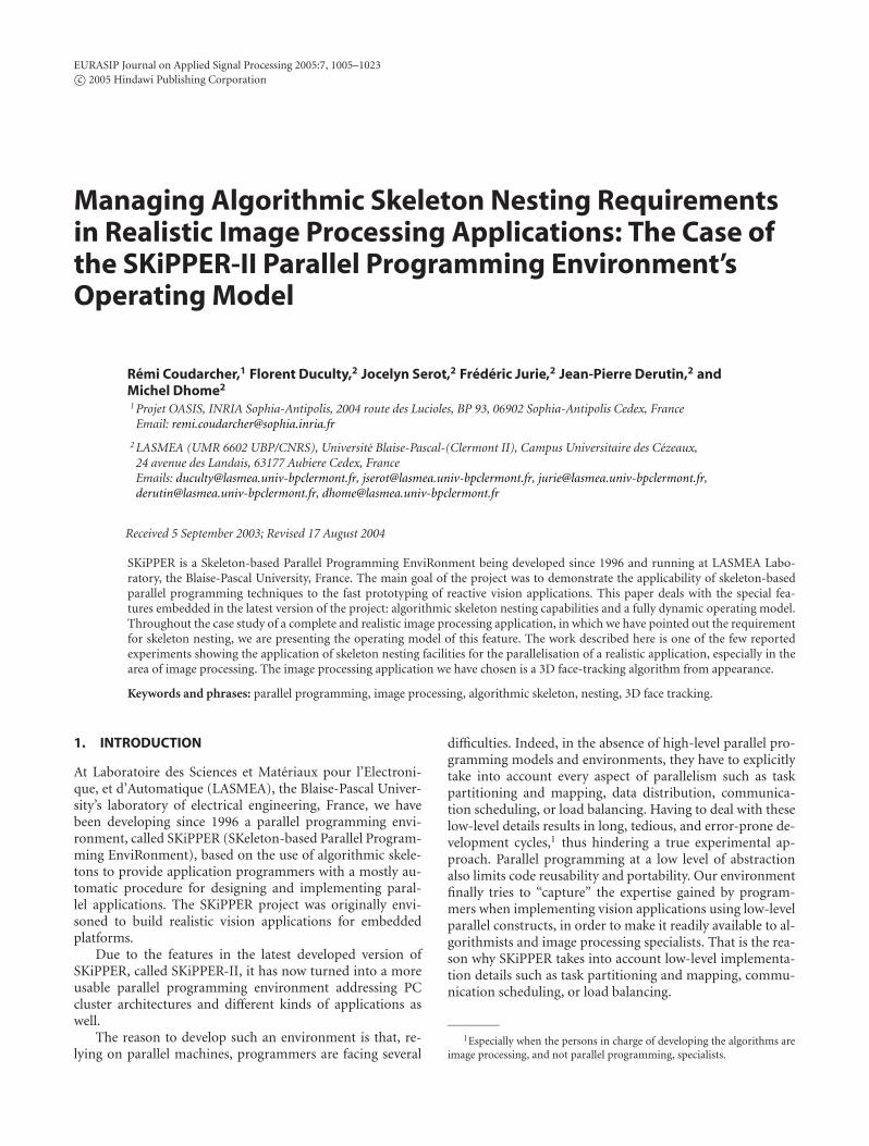
To obtain line Aθ of the interaction matrix relative to theorientation of the ellipse, we write down the following linearsystem:

∆i11 · · · ∆i1N...

. . ....

∆iM1 · · · ∆iMN

Aθ1

...AθN

=

∆θ1

...∆θM

, (1)

which can be shortly expressed as

M∆VI ∗ Aθ = ∆θ. (2)

The final solution is then obtained by

Aθ =(

Mt∆VIM∆VI

)−1Mt

∆VI∆θ =M+∆VI∆θ,

AXc =M+∆VI∆Xc,

AYc =M+∆VI∆Yc,

AR1 =M+∆VI∆R1.

(3)

The matrix M+∆VI is the so-called pseudoinverse of M∆VI .

3.5. Switching between reference views

Various reference appearences of faces can be tracked byswitching between views stored in our image base. In or-der to do that, we compare permanently the quadratic errorsof the tracking results between the currently tracked refer-ence pattern and its nearest neighbours in the learning base.The reference pattern giving the smallest error between itsshape vector and the current pattern sampled inside the cor-rected ellipse will be considered as the reference pattern tobe tracked in the next image. But, it is necessary to add anintermediate stage to compute the corrections on the pre-dicted position of the face in the image for each of the ref-erence patterns close to the currently tracked reference pat-tern in the collection of 2D views. For that, during the off-line learning stage, we compute, for the intermediate viewsplaced in the middle of the nearest reference patterns in thecollection of 2D images, the different positions of the ellipsecorresponding to the tracking results for each of the refer-ence patterns (Figure 18). We choose, in particular, these in-termediate images because we suppose that the change ofthe reference pattern, during the on-line tracking stage, hap-pens around these variations of the appearance. During thetracking phase, these different results are used with the pre-dicted parameters of the ellipse corresponding to the cur-rently tracked reference pattern to compute the predicted po-sitions of the face for the previous and next reference patternsin the current image before correction and estimation of theassociate quadratic error. In this additional stage, we use scaleand reference changes.

4. PARALLELISATION OF THE 3D FACE-TRACKINGALGORITHM USING ALGORITHMICSKELETON NESTING

4.1. Principle

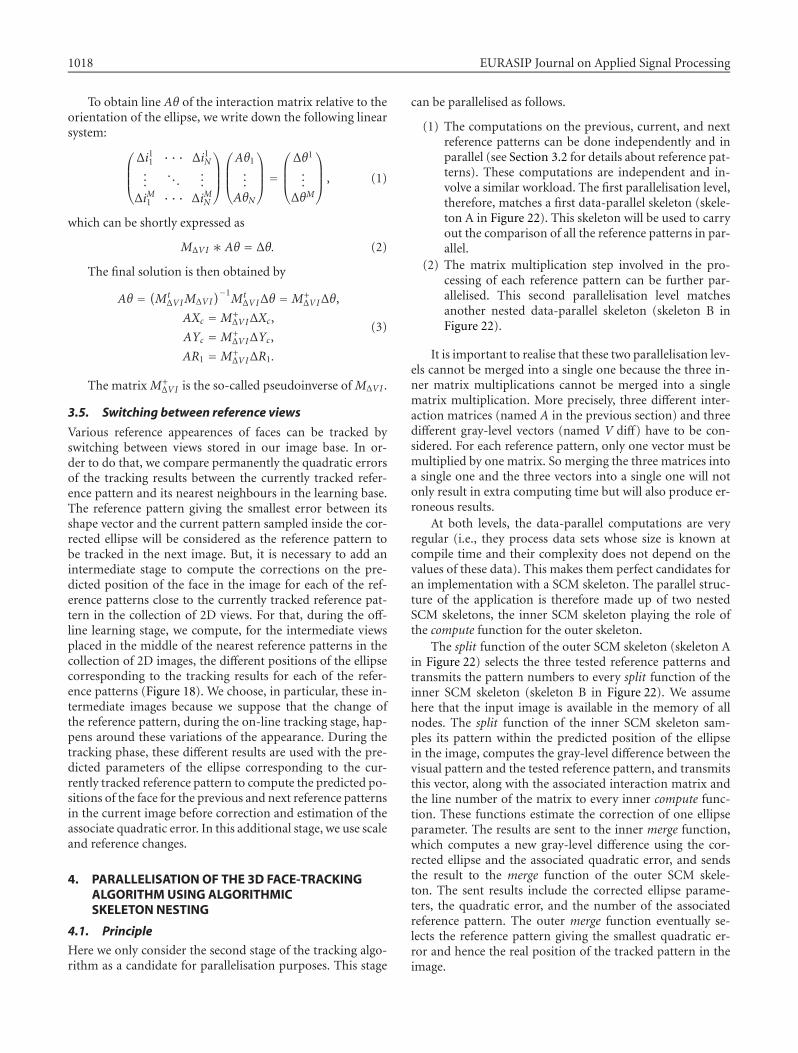
Here we only consider the second stage of the tracking algo-rithm as a candidate for parallelisation purposes. This stage

can be parallelised as follows.

(1) The computations on the previous, current, and nextreference patterns can be done independently and inparallel (see Section 3.2 for details about reference pat-terns). These computations are independent and in-volve a similar workload. The first parallelisation level,therefore, matches a first data-parallel skeleton (skele-ton A in Figure 22). This skeleton will be used to carryout the comparison of all the reference patterns in par-allel.

(2) The matrix multiplication step involved in the pro-cessing of each reference pattern can be further par-allelised. This second parallelisation level matchesanother nested data-parallel skeleton (skeleton B inFigure 22).

It is important to realise that these two parallelisation lev-els cannot be merged into a single one because the three in-ner matrix multiplications cannot be merged into a singlematrix multiplication. More precisely, three different inter-action matrices (named A in the previous section) and threedifferent gray-level vectors (named V diff) have to be con-sidered. For each reference pattern, only one vector must bemultiplied by one matrix. So merging the three matrices intoa single one and the three vectors into a single one will notonly result in extra computing time but will also produce er-roneous results.

At both levels, the data-parallel computations are veryregular (i.e., they process data sets whose size is known atcompile time and their complexity does not depend on thevalues of these data). This makes them perfect candidates foran implementation with a SCM skeleton. The parallel struc-ture of the application is therefore made up of two nestedSCM skeletons, the inner SCM skeleton playing the role ofthe compute function for the outer skeleton.

The split function of the outer SCM skeleton (skeleton Ain Figure 22) selects the three tested reference patterns andtransmits the pattern numbers to every split function of theinner SCM skeleton (skeleton B in Figure 22). We assumehere that the input image is available in the memory of allnodes. The split function of the inner SCM skeleton sam-ples its pattern within the predicted position of the ellipsein the image, computes the gray-level difference between thevisual pattern and the tested reference pattern, and transmitsthis vector, along with the associated interaction matrix andthe line number of the matrix to every inner compute func-tion. These functions estimate the correction of one ellipseparameter. The results are sent to the inner merge function,which computes a new gray-level difference using the cor-rected ellipse and the associated quadratic error, and sendsthe result to the merge function of the outer SCM skele-ton. The sent results include the corrected ellipse parame-ters, the quadratic error, and the number of the associatedreference pattern. The outer merge function eventually se-lects the reference pattern giving the smallest quadratic er-ror and hence the real position of the tracked pattern in theimage.


Image

Selection of tested reference patterns

Previous referencepattern processing

Current referencepattern processing

Next referencepattern processing

Sampling Sampling Sampling

Correction ofellipse parameters



Quadratic error Quadratic error Quadratic error

Skel

eto

nB

Skel

eto

nB

Skel

eto

nB

Skel

eto

nA

Result selection

Selected reference pattern

and real position of the tracked pattern in the image

Figure 22: General parallel structure.

4.2. Implementation

Once the parallel structure of the application has been iden-tified, the SKiPPER-II environment can be used to obtaina parallel implementation. From a programmer’s point ofview, this involves

(1) expressing this parallel structure using some kind ofdescription language (i.e., specifying which skeletonsare used and in what order),

(2) providing the application-specific sequential functionsto be used as arguments to the skeletons.

In previous SKiPPER versions, expressing the parallel struc-ture was carried out using a subset of the Caml language [4].The same approach is intended to be used for SKiPPER-II.In this case, the intermediate description of the application(as a tree of TF/II skeletons) will be generated by a modifiedversion of the Camlflow tool [19]. In the current version ofSKiPPER-II, this step is still handled manually, that is, theintermediate description is provided by the programmer inthe form of a C descriptor which can be used directly by thekernel. This descriptor encodes, in the form of a C array, thetree of TF/II skeletons that matches the skeletal structure ofthe application. For the tracker application, the correspond-

#define SKL NBR 2SK2 Desc app desc [SKL NBR] ={{ SKO, END OF APP, MASTER, SK1 },

{ SK1, UPPER, SLAVE, NIL }};

Algorithm 4: Encoding the parallel structure of the tracker appli-cation. C encoding for SKiPPER-II.

ing descriptor5 is given in Algorithm 4 (Figure 23 recalls theskeletal structure of the application). There is one line perskeleton. On each line,

(i) the first column is the skeleton ID (for reference),

(ii) the second column indicates the skeleton “continua-tion,” that is, whether its results must be sent to an up-per level or to another skeleton at the same level,6

(iii) the third column tells whether this skeleton acts as aslave (i.e., is nested) or as a master,

5This is a slightly edited version—for readability—of the actual code.6Here, END OF APP is a special case meaning that the current skeleton

is the last one.


S1

S2

F2

M2

M1

F2 F2 F2 F2 F2 F2 F2 F2 F2 F2 F2

S2 S2

M2 M2

Original application using SCM skeletons

Inn

erSC

Msk

elet

on

(ske

leto

nB

)

Ou

ter

SCM

skel

eto

n(s

kele

ton

A)

S1M1

S2M2

S2M2

S2M2

F2 F2 F2 F2 F2 F2 F2 F2 F2 F2 F2 F2

Internal TF/II treecorresponding to the

intermediate description

Support process User sequential function

Inn

erT

F/I

Isk

elet

on

(ske

leto

nB

)

Ou

ter

TF

/II

skel

eto

n(s

kele

ton

A)

S1: Selection of tested reference patterns

S2: Sampling

M1: Result selection

F2: Correction of ellipse parameters

M2: Quadratic error

Figure 23: Encoding the parallel structure of the tracker application. Graphical representation.

(iv) the last column gives the ID of the destination skele-ton.

The second step in using SKiPPER-II is providing theapplication-specific sequential functions. These functions—to be used as arguments to the specified skeletons—are writ-ten in C and must be “pure” functions (no side-effect, noreference to global variables or shared data). All nonatomicarguments7 must be passed by address and all results must bereturned by address. The prototypes of the sequential func-tions for the tracker application are given in Algorithm 5.

In the current implementation of SKiPPER-II, the pro-grammer is also required to write a few lines of stub codeto allow the application-specific sequential functions to belinked with the kernel code. The main role of this stub codeis to alleviate the lack of support for data polymorphism inthe C language (at the kernel level, all application-specificfunctions must have a uniform interface, in which all argu-ments and results are passed/returned as untyped buffers).This stub code is very systematic and repetitive (it essentially

7By atomic arguments, we mean those having nonstructured data types,such as int, float, and so forth.

consists in packing/unpacking application-level data struc-tures into/from kernel-level (char ⋆) arrays) and could beautomated.

5. RESULTS AND DISCUSSION

The benchmark was performed on Intel Celeron Beowulfmachine (32× 533 MHz nodes, 100 Mbps switched Ethernetnetwork). Figures 24 and 25, respectively, show the comple-tion time of the algorithm and the relative speedup obtainedin increasing the number of nodes for two quantities of sam-pled points in the elliptic area (170 and 373 sample points).

It must be noticed that using more than 170 sample is notgiving better results in terms of tracking capabilities (using170 points already provides a sufficiently robust tracking).This number was increased in order to further assess the per-formances of SKiPPER-II kernel, since it directly influencesthe computation/communication ratio.

The curves in Figures 24 and 25 exhibit three phaseswhich can be related to the behaviour of the SKiPPER-II ker-nel.

The first phase is observed for 1 to 2 nodes (373 sam-pled points) or 1 to 3 nodes (170 sampled points): here the


S1(

int pattern number, /⋆I ⋆/Ellipse current ellipse, /⋆I/O⋆/int ⋆⋆ tracker number to test /⋆ O⋆/

);

S2(

Ellipse current ellipse, /⋆I/O⋆/int tracker number to test, /⋆I/O⋆/int ⋆ gray level vector size, /⋆ O⋆/float ⋆⋆gray level difference-vector, /⋆ O⋆/int ⋆⋆matrix line number, /⋆ O⋆/float ⋆⋆⋆matrix /⋆ O⋆/

);

F2(

Ellipse current ellipse, /⋆I/O⋆/int tracker number to test, /⋆I/O⋆/int gray level vector size, /⋆I ⋆/float ⋆ gray level difference-vector, /⋆I ⋆/int matrix line number, /⋆I/O⋆/float ⋆ matrix, /⋆I ⋆/float ⋆ correction /⋆ O⋆/

);

M2(

Ellipse current ellipse, /⋆I ⋆/int tracker number to test, /⋆I/O⋆/int matrix line number, /⋆I ⋆/float correction /⋆I ⋆/float ⋆ quadratic error, /⋆ O⋆/Ellipse ⋆ corrected ellipse, /⋆ O⋆/

);

M1(

Ellipse current ellipse, /⋆I ⋆/int tracker number to test, /⋆I ⋆/float quadratic error, /⋆I ⋆/Ellipse ⋆ final current ellipse, /⋆ O⋆/int ⋆ final pattern number /⋆ O⋆/

);

Algorithm 5: Signature of the application-specific sequential func-tions for the tracker application.

completion time is higher in the multiprocessor case. Thisnegative speedup can be explained by the way the outer SCMskeleton is deployed on the network. In fact, with the run-time mechanism presented in Section 2.4, using two nodesdoes not provide more computing power but only createscommunications. This is because one of the nodes is usedas a dispatching process and is not performing useful com-putation at all. When the computation versus communi-cation is small (as in the 170 points case), this effect caneven be observed with 3 nodes because the time to com-municate data to the two nodes doing computations de-stroys the potential gains of performing theses computationsis parallel.

55

50

45

40

35

30

25

20

15

10

5

01 3 5 7 9 11 13 15 17 19 21 23 25

Number of nodes

Co

mp

leti

on

tim

e(m

s)

170 sampled points

373 sampled points

Figure 24: Completion time for 170 and 373 sampled points for 3Dface-tracking algorithm parallelisation on an Intel Celeron Beowulfmachine.

25

20

15

10

5

01 3 5 7 9 11 13 15 17 19 21 23 25

Number of nodes

Spee

du

p

Linear

170 sampled points

373 sampled points

Figure 25: Speedup for 170 and 373 sampled points for 3D face-tracking algorithm parallelisation on an Intel Celeron Beowulf ma-chine.

From 4 to 19 nodes, performance increases with thenumber of nodes (though not linearly). This phase corre-sponds to the deployment of the inner SCM skeleton, whichperforms the vector-matrix multiplications in parallel.

The last phase starts with 19 nodes. Here, increasing thenumber of computing nodes does not improve performance.This can be explained by the fact that the each SCM skeletonencapsulates a fixed data-parallel strategy. The maximum ef-ficiency is reached when the number of available processing


nodes matches this fixed parallelism degree.8 When the num-ber of available nodes is higher (19–32), no further paral-lelism can be exploited and hence efficiency decreases. Whenthe number is smaller (4–18), the kernel sequentialises someprocessings on some nodes (thus providing a form of “virtu-alisation” mechanism).

The relatively poor results in terms of efficiency can bemore generally explained by the relatively small computa-tion versus communication ratio of the parallel version. Asa matter of fact, the sequential version of the algorithm wasalready very efficient because of very few intensive comput-ing stages. This is especially true for the inner parallelisationlevel because the matrix multiplication is only a (p×N) ma-trix multiplied by the gray-level vector of size N .

6. CONCLUSION

This paper presents a skeleton-based parallel programmingenvironment supporting skeleton nesting and the paralleli-sation of a realistic image processing application using thislatest capability. As far as we know, the work described hereis one of the few reported experiments showing the applica-tion of skeleton nesting facilities for the parallelisation of arealistic application, especially in the area of image process-ing. Indeed the 3D face-tracking algorithm cannot be entirelyparallelised without this kind of skeleton combination. Thisis due to the fact that the different parallelisation levels can-not be merged into a single one and have to be handled byseparate nested skeletons.

However, this work also shows that the run-time mech-anism used in SKiPPER-II entails a significant performancepenalty, especially when the computation versus communi-cation ratio is low. In this case, skeleton nesting is not a trans-parent operation in terms of efficiency.

As for methodological aspects, we noticed that the par-allelisation of the tracking algorithm only required three tofour working days. This time was mainly dedicated to se-lect the right parallelisation structure (which skeletons andhow are they connected), and subsequently to split the orig-inal algorithm into computing functions to plug into theskeletons (the original user’s functions have to be splited andtheir interface rewritten). Concerning parallelisation choicesfor the 3D face-tracking algorithm, we think that after thisexperiment, it could be interesting to parallelise the firststage of the algorithm, although it is normally an “off-line”stage. The reason is that decreasing the completion timewill bring the opportunity to use all of the processing stagesin an “on-line” way in order to use the tracking algorithmfor multitarget tracking purposes, like multivehicle track-ing [20]. In this case, speeding up this stage could allowthe application to learn reference patterns of vehicles on thefly and hence allow it to adapt itself to the road environ-ment without relying on a large prebuilt database of pat-terns.

8For the outer SCM skeleton, the optimal number of nodes is 4 (3 forcomputing, one for dispatching); for the inner one, this number is 5 (4 + 1).

ACKNOWLEDGMENTS

The authors would like to acknowledge the support of theEuropean Commission through Grant number HPRI-1999-CT-00026 (the TRACS Programme at EPCC, Scotland) andto thank the staff members of the Department of Comput-ing and Electrical Engineering, the Heriot-Watt University,Edinburgh, Scotland. The authors would also like to thankSantosh Anand, a Graduate from IIT Kampur, India, for hiscareful review of the paper’s English.

REFERENCES

[1] D. Ginhac, J. Serot, and J.-P. Derutin, “Fast prototyping ofimage processing applications using functional skeletons onMIMD-DM architecture,” in IAPR Workshop on Machine Vi-sion Applications, pp. 468–471, Chiba, Japan, November 1998.

[2] D. Ginhac, Prototypage rapide d’applications paralleles de vi-sion artificielle par squelettes fonctionnels, Ph.D. thesis, Univer-site Blaise-Pascal, Clermont-Ferrand, France, January 1999.

[3] J. Serot, D. Ginhac, and J.-P. Derutin, “Skipper: a skeleton-based parallel programming environment for real-time im-age processing applications,” in 5th International Conferenceon Parallel Computing Technologies (PACT ’99), V. Malyshkin,Ed., vol. 1662 of Lecture Notes in Computer Science, pp. 296–305, Springer-Verlag, Petersburg, Russia, September 1999.

[4] J. Serot, D. Ginhac, R. Chapuis, and J.-P. Derutin, “Fast pro-totyping of parallel-vision applications using functional skele-tons,” Machine Vision and Applications, vol. 12, no. 6, pp. 271–290, 2001.

[5] R. Coudarcher, J. Serot, and J.-P. Derutin, “Implementationof a skeleton-based parallel programming environment sup-porting arbitrary nesting,” in 6th International Workshop onHigh-Level Parallel Programming Models and Supportive Envi-ronments (HIPS’01), F. Mueller, Ed., vol. 2026 of Lecture Notesin Computer Science, pp. 71–85, Springer-Verlag, San Fran-cisco, Calif, USA, April 2001.

[6] M. Hamdan, G. Michaelson, and P. King, “A scheme for nest-ing algorithmic skeletons,” in Proc. 10th International Work-shop on Implementation of Functional Languages (IFL ’98),C. Clack, T. Davie, and K. Hammond, Eds., pp. 195–212, Lon-don, UK, September 1998.

[7] G. Michaelson, N. Scaife, P. Bristow, and P. King, “Nested al-gorithmic skeletons from higher order functions,” Parallel Al-gorithms and Applications, vol. 16, no. 2-3, pp. 181–206, 2001,Special issue on high level models and languages for parallelprocessing.

[8] M. Hamdan, A Combinational framework for parallel pro-gramming using algorithmic skeletons, Ph.D. thesis, Heriot-Watt University, Department of Computing and ElectricalEngineering, Edinburgh, UK, January 2000.

[9] F. Jurie and M. Dhome, “A simple and efficient templatematching algorithm,” in Proc. 8th IEEE International Con-ference on Computer Vision (ICCV ’01), vol. 2, pp. 544–549,Vancouver, BC, Canada, July 2001.

[10] M. Cole, Algorithmic Skeletons: Structured Management of Par-allel Computation, Pitman/MIT Press, London, UK, 1989.

[11] M. Cole, “Algorithmic skeletons,” in Research Directionsin Parallel Functional Programming, K. Hammond and G.Michaelson, Eds., pp. 289–303, Springer, UK, November1999.

[12] J. Serot, “Embodying parallel functional skeletons: an exper-imental implementation on top of MPI,” in 3rd Intl Euro-ParConference on Parallel Processing, C. Lengauer, M. Griebl, andS. Gorlatch, Eds., pp. 629–633, Springer, Passau, Germany,August 1999.


[13] N. Scaife, A dual source parallel architecture for computer vi-sion, Ph.D. thesis, Heriot-Watt University, Department ofComputing and Electrical Engineering, Edinburgh, UK, May2000.

[14] T. Grandpierre, C. Lavarenne, and Y. Sorel, “Optimized rapidprototyping for real-time embedded heterogeneous multipro-cessors,” in Proc. IEEE 7th International Workshop on Hard-ware/Software Codesign (CODES ’99), pp. 74–79, Rome, Italy,May 1999.

[15] W. Gropp, E. Lusk, N. Doss, and A. Skjellum, “A high-performance, portable implementation of the MPI messagepassing interface standard,” Parallel Computing, vol. 22, no. 6,pp. 789–828, 1996.

[16] R. Coudarcher, Composition de squelettes algorithmiques: ap-plication au prototypage rapide d’applications de vision, Ph.D.thesis, LASMEA, Blaise-Pascal University, Clermont-Ferrand,France, December 2002.

[17] G. D. Hager and P. N. Belhumeur, “Efficient region trackingwith parametric models of geometry and illumination,” IEEETrans. Pattern Anal. Machine Intell., vol. 20, no. 10, pp. 1025–1039, 1998.

[18] F. Dellaert and R. Collins, “Fast image-based tracking by se-lective pixel integration,” in International Conference on Com-puter Vision Workshop on Frame-Rate Vision, Corfu, Greece,September 1999.

[19] J. Serot, “Camlflow: a caml to data-flow translator,” in Trendsin Functional Programming. Volume 2, S. Gilmore, Ed., pp.129–141, Intellect Books, Bristol, UK, 2001.

[20] F. Marmoiton, F. Collange, P. Martinet, and J.-P. Derutin, “Areal time car tracker,” in Proc. International Conference on Ad-vances in Vehicle Control and Safety (AVCS ’98), pp. 282–287,Amiens, France, July 1998.

Remi Coudarcher is a computer science engineer. He graduatedfrom ISIMA, France, and received his Ph.D. degree in computerscience from Blaise-Pascal University, France. He has been a post-doc fellow at INRIA, France. His research interests include parallelimage processing, and methodologies for parallel and distributedprogramming and grid computing.

Florent Duculty is an engineer in electrical science. He graduatedfrom CUST, France, and has a Ph.D. degree in computer sciencefrom Blaise-Pascal University, France. His research interests includeimage processing applied to robotics motion by visual servoing.

Jocelyn Serot is an Associate Professor in electrical engineering atBlaise-Pascal University, France. His research interests are in the de-velopment and use of methodologies for parallel programming, es-pecially in the field of image processing.

Frederic Jurie is a Researcher at CNRS, France. His researches areconcerned with image processing, especially movement and objectdetection, and image recognition from appearance.

Jean-Pierre Derutin is a Full Professor in electrical engineering atBlaise-Pascal University, France. His research interests are in the de-sign of dedicated and embedded parallel computers for real-timeimage processing.

Michel Dhome is a Director of Research at CNRS and Codirectorof the LASMEA Laboratory, France. His researches include imageprocessing for automatic recognition and robotics.

managing algorithmic skeleton nesting requirements in

Documents