MANAGEMENT PERSPECTIVE

Accurate measurement of suspended sediment concentration is important

for application in a wide range of engineering and environmental problems. The

Water Survey of Canada uses about 600 suspended sediment samplers in its

national data collection program. Their calibration requires significant time

and resources. Regular calibrations of the samplers are to be conducted in the

towing tank at the National Water Research Institute in Burlington, Ontatio.

To facilitate the sampler calibrations, a static head test facility was

developed to calibrate sampler nozzles for use with a particular type of

sampler. In addition, the facility will be used to conduct development research

on sampler calibrations. This report completes the first stage of the sampler

calibration strategy presented by Engel and Zrymiak (1989).

Dr. J . Lawrence Director

Research and Applications Branch

PERSPECTIVE llE GESTION \

9 a n s l e <:as d 'un grand 6van t , a i l d e c!uc+stioil er~vironrienierrti:l .~~; ~t d ' i . n g & n i e r i e , i l impor-t e d ' o h t e n i r d e s rriesures p r e c i s e s d e c o n c e n t r a t i o n dc. si?climc+nt,s e n suspens i . on . En v e r t a rie s o n programme na Linnt-11 d c c o l l e r t e d e s donnees? les r e s p o n s a h l e s d e s He ieves h v d r o l o g i q u e s du Canada u t i l j s e n l e n v i r o n 600 6 c h a n t . i l l c ) n n e u r s de s4diment .s e n s n s p e n s i on . I,' Ctt a1 orlriagr d e ces C c h a n t i l l o n n e u r s dernande beaucoup d e temps et. d e r e s s o u r c e s . On p r o c e d e r a a 1' k t a lonnag t - r P g u l i e r d e s 6 c h a n t i l l o n n e u r s d a n s l e b a s s i n d e h a l a g e d e 1 ' T n s t i t u t n a t i o n a l d e l a r e c h e r c h e sur . ips eaux d e R u r l i n g t o n (Ontar- io: .

A f i n tit- : f r - t c : i i i t . e r 1 ' 4t :-11 onrrtl!ge C I ~ S b c h a n t i l l o n n e u ~ ~ : on :=I t;l ahorc; un d i s p o s i t i f d ' e s s a i s d e c h a r g e s t a t i q ~ i e p e r m e t t a n t d 7 6 t a l n n n e r . les b u s e l - u r e s ut..i l . i s 8 e s dans rlri t y p e d 6 f i n i d 7 6 c h a n t i l l o n n e u r . En o u t r e t n e d i s p o s i t i f s e r v i r a d a n s d e s r e c h e r c h e s d e developpement sur. 1 ' 6 t a l o n n a g e d ' e c h a n t il l o n n e u r s . 1,e p r 6 s e a t r a p p o r t compli+t.e l a p r e m i & r e P t a p e de l a strategic d 7 6 t a l o n n a g e d ' e c h a n t i l l o n n e u r s p r e s e n t e e p a r Engel et Zrymiak ( 1 9 8 9 ) .

J . Lawrence If i rect tellr D i r e c t .ion de l a re r :herche et- rles app l i c a t , i o n s .

The method of calibrating suspended sediment sampler nozzles has been

examined using theoretical and dimensional analysis and experimental

measurements. Based on the results, a static head nozzles test facility was

designed and built. The facility will be used to calibrate nozzles for suspended

sediment samplers commissioned for field use, and to conduct tests on other

pertinent factors which may affect the performance of sampler nozzles.

.On a 6tudit5 la methode d96talonnage des buselures d'6chantillonneurs de sediments en suspension, en ayant recours a une analyse theorique et dimensi onnell e, ainsi qu' a des mesures exp6rimentales. Les result at.s ont permis de mettre au point un dispositif d'essais de charge stat.ique. Ce dispositif servira ii gtalnnner les buselures dans le cas des echantillonneurs de sediments en suspension commandes pour le terrain, ainsi qu'a mener des essais sur d'autres GlGments pertinents qui pourraient entraver l e fonctionnement des t)uselures d'echantillonneurs.

TABLE OF CONTENTS

PAGE

MANAGEMENT PERSPECTIVE

1.0 INTRODUCTION

2.0 METHOD OF TESTING SEDIHENT SAMPLERS 2 .1 Preliminary Considerations 2 .2 Method of Altering the Value of K 2 .3 Calibration of the Nozzles

3.0 BASIC PRINCIPLES OF THE STATIC HEAD METHOD 3 . 1 General Equation for Velocity Coefficient 3 .2 Friction Factor 3.3 The Nozzle Energy Loss Coefficients 3 .4 Behaviour of the Velocity Coefficient

4.0 DESIGN OF STATIC HEAD TEST FACILITY 4 . 1 General Design Considerations 4 . 2 The Nozzle Test Chamber 4 . 3 The Constant Head Tank 4 . 4 Stilling Well

5.0 PRELIMINARY TESTS 5 . 1 Procedure 5 .2 Data Analysis

6 . 0 CONCLUSIONS

ACKNOWLEDGEMENTS

iii

REFERENCES

TABLES

FIGURES

1.0 INTRODUCTION

The accuracy of all suspended sediment samplers must be checked

regularly to ensure that reliable data are obtained. Samplers are tested in a

towing tank with a particular set of nozzles as a total system. In addition to

the properties of the sampler body itself, the sampler performance is sensitive

to the geometric and thus the hydraulic characteristics of the nozzles. In

practice, nozzles often get damaged causing changes in their hydraulic

characteristics, thus requiring their replacement.

The nozzles can be calibrated seperately or the sampler can be adjusted

to be compatible with a given nozzle (Engel and Zrymiak, 1989). The calibration

of the sampler nozzles must have a high degree of repeatability and must cover

the range of nozzle velocities encountered under normal sediment sampling

conditions. For this purpose a new constant head test facility was constructed

in the Hydraulics Laboratory of the National Water Research Institute (NWRI).

This new facility will be used to maintain quality control of all nozzles used

by the Water Survey of Canada (WSC) in their national sediment measuring

program. The test facilty is part of a calibration plan presented by Engel and

Zrymiak (1989) and was designed and fabricated by the Research and Applications

Branch (RAB) of the NWRI in support of the Sediment Survey Section of the WSC at

headquarters in Ottawa. The funds for the fabrication of the test facility were

provided by the Sediment Survey Section.

HETHOD OF TESTING SEDIHFST SAMPLERS

Preliminary Considerations

The suspended sediment samplers operate on the premise that the

velocity of flow through the nozzle is equal to the velocity of the streamflow

surrounding the nozzle. This is known as iso-kinetic sampling. Samplers are

tested to ensure that this condition is achieved within an acceptable margin of

error. For the purpose of sediment sampling control, the nozzle velocity and

the streamflow velocity are expressed as a ratio given by

where K = the sampler coefficient, V, = the velocity in the nozzle and V, = the

streamflow velocity. The aim of the sampler tests is to achieve a value of K

sufficiently close to 1.

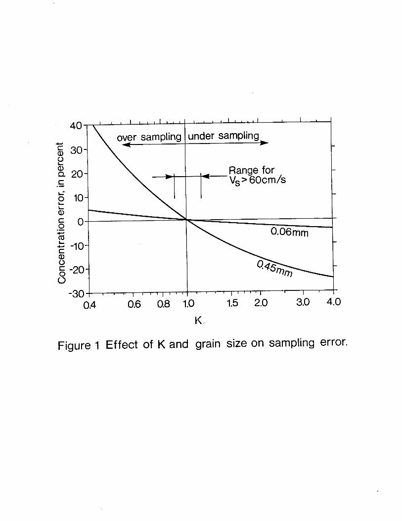
The value of K has direct implications on the accuracy of sampling

suspended sediment. When K > 1 the sampler will undersample suspended sediment

concentration, whereas when K < 1, the sampler will oversample as shown in

Figure 1 (Beverage and Futrell, 1986). The error in sampling the sediment

concentration has been shown to vary with particle size. When sediments are in

the silt and clay size (i.e. particle diameter < .06 mm) the error in sampling

is within 5% if the sampler coefficient is in the range 0.4 < K < 4.0. In

contrast to this, when the sediment is in the sand size range, the sampling

accuracy is very dependent on the value of K. It can be seen in Figure 1, that

for a grain size of 0.45 mm, values of K must be in the range 0.88 < K < 1.20 in order to maintain a sediment concentration accuracy of 5%. At first glance it

would appear that for sampling of suspended sediment in the clay to silt sizes,

adjustment of the samplers is not so critical. However, one must keep in mind

that the sediment particle size is a function of the flow velocity. It can be

seen from Figure 1 that for velocities as low as 60 cm/s, sediments can be

expected to be in the sand sizes for which errors in the measurement of sediment

concentrations is strongly dependent on the value of K. Therefore, it is

important to ensure that the sediment samplers are adjusted as close as possible

to the ideal value of K = 1.0.

The value of K for a given sampler depends on both the characteristics

of the sampler body itself and the characteristics of the nozzle. Samplers are

tested in a towing tank over the range of velocities encountered in the field.

Tests by Beverage and Futrell (1986) have shown that results from tests

in towing tanks are not significantly different from results of tests conducted

in turbulent flows in flumes. For each towing velocity, a water sample is

collected over the measured time interval required to fill the sample bottle

about 3/4 full. Care is taken that the sampler is equipped with the appropriate

size of nozzle for the selected towing velocity. Using the collected sample the

velocity of the flow through the nozzle is computed and and values of K are

determined. If all values of K are sufficiently close to 1.0, then the tests in

the towing tank are considered to be successful. Alternatively, if values of K

are either smaller or larger than desirable, then additional steps must be

taken.

Method of Altering the Value of K

In order to improve the sampler performance, it is recognized that the

value of K may be influenced by changes to either the sampler body itself, the

nozzle or both. If K < 1.0, the sampler intake velocity must be increased and

in most cases this can be achieved by making suitable modifications to the

nozzle or the air exhaust passages in the sampler body. Experience has shown

that the most effective way of increasing the nozzle velocity is to change the

nozzle outlet geometry (Beverage and Futrell, 1986). Careful reaming and

chamfereing of the nozzle outlet will reduce the energy losses to permit

sufficient increase in the nozzle velocity, thereby increasing the value of K.

In contrast to this, a value of K > 1.0 may be corrected by making adjustments

to the sampler by reducing the size of the air exhaust tube or the exhaust port

in the sampler body, thereby increasing the energy losses in the sampler. This

method is not always successful. Benson (1981) reports instances where it has

been impossible to make sufficient adjustments to obtain an acceptable value of

K. Under such circumstances a sediment sampler cannot be used.

Sampler testing in a towing tank is very time consuming and expensive.

Therefore, once the initial value of K has been obtained, any changes to the

nozzles should be evaluated and made by alternate means.

2.3 Calibration of the Nozzles

A review of WSC sampler calibration methods by Engel and Zrymiak

(1989), showed that nozzles were calibrated separately using a static hydraulic

head obtained with a constant head tank. In using such a static head method it

must be recognized that the flow field at the nozzle entrance for the cases of

streamflow and static head are different.

When the sampler is placed into the streamflow, the flow approaches the

nozzle on a broad front. If K = 1, the streamflow will pass straight into the

nozzle while any stream lines on either side of the nozzle intake will be

deflected as shown in Figure 2(a). For this condition the trajectories of the

sediment particles are parallel to the streamlines of the flow entering the

nozzle. As a result the sampler collects the correct proportions of water and

sediment particles. When K < 1.0, the velocity in the nozzle will be slower

than the streamflow velocity and as a result, an area of stagnation will develop

at the head of the nozzle as shown in Figure 2(b). In this case the stream

lines of the approaching flow will be deflected ahead of the nozzle entrance.

However, the sediment particles, because of their inertia, will tend to continue

on their original path toward the nozzle entrance. As a result, for a given

sampling time, the sampler will undersample the water volume but collect a

larger proportion of sediment particles, resulting in oversampling of the

sediment concentration. Finally, when K > 1.0, the velocity in the nozzle will be greater than that of the approaching flow and streamlines in the vicinity of

the nozzle intake will converge toward the intake as shown in Figure 2(c). Once

again the sediment particles will resist the sudden change in direction and the

increase in water flow through the nozzle will not be accompanied by a

corresponding increase in sediment particles. As a result, in this case the

sampler will undersample the sediment concentration. In contrast to this, when

the nozzle is under a static head, the flow field around the nozzle intake is

generated by the flow passing through the nozzle itself. Accordingly, water

will be drawn toward the nozzle inlet in a manner represented schematically by

the stream lines shown in Figure 3. Fortunately, the difference in the flow

fields is only felt at the head of the nozzle. From the nozzle intake

downstream, the flow dynamics are the same regardless of the external flow

conditions. Therefore, as long as the geometry of the nozzle head is always the

same, any alterations to the nozzles to improve the value of K can be made

downstream of the inlet. This approach is in agreement with methods reported by

Beverage and Futrell (1986) and Benson (1981). These observations confirm that

the static head method may provide an efficient way of completing the sampler

evaluation without the use of the towing tank.

3.0 BASIC PRINCIPLES OF THE STATIC HEAD HETHOD

3.1 General Equation for Velocity Coefficient

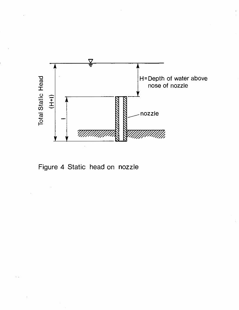
It can be shown from energy considerations, with reference to the

schematic layout in Figure 4, that without energy losses, the velocity of the

flow passing through a nozzle is given by

where V, = theoretical velocity of the flow through the nozzle, H = the depth

of water above the nozzle entrance, 1 = the length of the nozzle and g = the

acceleration due to gravity. The velocity V, is known as the ideal velocity.

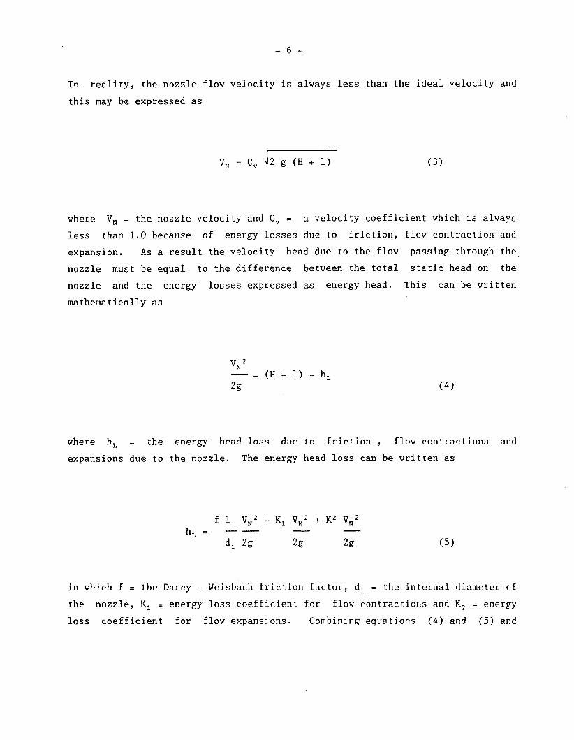
In reality, the nozzle flow velocity is always less than the ideal velocity and

this may be expressed as

where V, = the nozzle velocity and C, = a velocity coefficient which is always

less than 1.0 because of energy losses due to friction, flow contraction and

expansion. As a result the velocity head due to the flow passing through the

nozzle must be equal to the difference between the total static head on the

nozzle and the energy losses expressed as energy head. This can be written

mathematically as

where h, = the energy head loss due to friction , flow contractions and

expansions due to the nozzle. The energy head loss can be written as

in which f = the Darcy - Weisbach friction factor, di = the internal diameter of

the nozzle, K, = energy loss coefficient for flow contractions and K, = energy

loss coefficient for flow expansions. Combining equations (4) and (5) and

solving for V, results in

If one now compares equation (3) and (6), one observes that the velocity

coefficient C, can be expressed as

Friction Factor

The friction factor can be expressed in functional form as

where 4 denotes a function, E = the height of the surface roughness of the flow

boundary in the nozzle, v = the kinematic viscosity of the fluid, p = the

density of the fluid and u = the surface tension of the fluid. Using

dimensional analysis, equation (8) can be reduced to the following dimensionless

form:

where +, denotes another function. Troskolanski ( 1 9 6 0 ) states that for conduits

with di < 1 .25 cm, surface tension of the fluid must be taken into account. The

values of d, for the sampler nozzles are 3 .2 mm, 4.8 mm and 6 . 4 mm, all of which

are significantly smaller than the minimum diameter given by Troskolanski

( 1 9 6 0 ) . However, velocities of flow through the nozzles vary from about 0 .5 m/s

to 3.0 m/s. The heads required to obtain such velocities are large enough to

make surface tension effects negligibly small. Therefore, equation ( 9 ) can be

reduced to the more familiar form

where +, denotes another function.

The solution to equation ( 1 0 ) is available in the practical form of the

Moody Diagram given in Figure 5 . From this diagram, values of the friction

factor can be obtained for known values of the relative roughness and the

Reynolds number. Data from Engel and Zrymiak ( 1 9 8 9 ) show that over the

practical range of nozzle velocities, Reynolds numbers vary from 5000 to 10,000.

This range is indicated on the Moody Diagram in Figure 5 . Examination of the

curves in Figure 5 reveals that in this range of Reynolds numbers, flows through

the nozzles are always in the smooth turbulent regime. As a result,

considerable changes in the relative roughness of the nozzle flow boundary will

result in very small changes in the friction factor f. This suggests that,

variations in roughness of the nozzle flow passages will not have an adverse

effect as long as the imperfections do not significantly affect the

cross-sectional area of the flow. For the three sizes of brass nozzles used,

values of e/di vary from 0.0002 to 0.0004 for which values of f are not

significantly different. Therefore, for the case of sampler nozzles, one may

consider that f is a function of the Reynolds number only, varying from 0.038

when Re = 5000 to 0.031 when Re = 10,000. A similar result can be expected for

plastic nozzles.

3 . 3 The Nozzle Energy Loss Coefficients

The energy loss coefficients K, and K, represent the entrance losses

and the exit losses respectively. The entrance loss coefficient K, can be

expected to be dependent on the entrance geometry and fluid properties. This

can be expressed in functional form as

where 4, denotes a function, r = the radius of curvature of the entrance lip,

do = the outside diameter of the nozzle and all other variables have already

been defined. Using dimensional analysis, equation (11) can be reduced to the

f orm

where +4 denotes another function. The sampler nozzle is similar to a

re-entrant intake (Simon, 1986). Values of K, for the intake shape of the

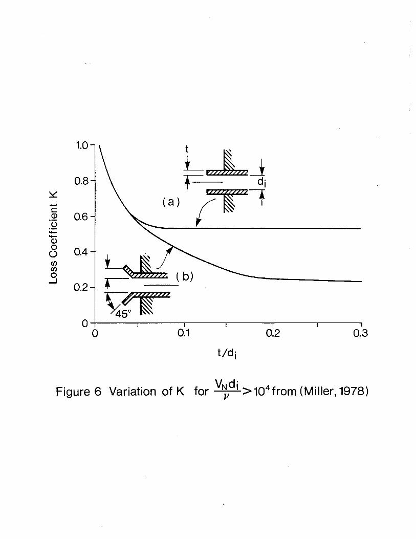
sampler are not available. However data from Miller (1978) indicates that for a

sharp edged intakes at Reynolds numbers above 10,000, values of K, vary as shown

in Figure 6. The curve shows that K, is strongly dependent on the wall thick-

ness to inside diameter ratio t/di when this is less than about 0.08. When t/di

> 0.08, K, is constant at about 0.5, indicating that wall thickness for

sediment sampler nozzles is not important. The value of K, can be reduced by

bevelling the intake edge. This can also be seen in Figure 6, which gives

values of Kl for a bevel angle of 45 degrees. In this case the thickness of the

nozzle wall is more important and K, varies significantly with t/di for values

of t/di < 0.2. For sampler nozzles values of t/di > 0.2 and the effect on K1 is only minor. These results show that some increase in the efficiency of intakes

can be obtained by making modifications to the geometry of the intake. However,

for the sediment samplers, values of Reynolds numbers are in the range from 5000

to 10,000 which are about one order of magnitude lower than the minimum Reynolds

number for which the curves in Figure 6 are valid. Therefore, one can expect

some dependency of K, on the Reynolds number in the operating range of the

sampler nozzles, although the relationship is not known.

The energy loss coefficient for the nozzle outlet can be expressed in a

general functional form as

where +5 denotes a function, 8 = the angle of expansion of the nozzle outlet and

the remaining variables have already been defined:Using dimensional analysis

equation (13) can be reduced to the more meaningful dimensionless form

where $, denote another function. The relative nozzle wall thickness d,/di is

not expected to be important and can be removed from further considerat ion.

Therefore, K, can be expressed in the final dimensionless form as

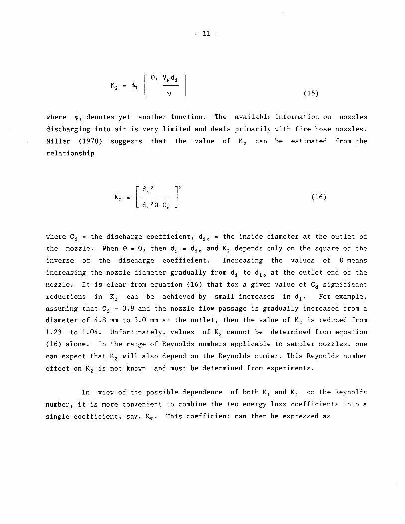
where +, denotes yet another function. The available information on nozzles

discharging into air is very limited and deals primarily with fire hose nozzles.

Miller (1978) suggests that the value of K2 can be estimated from the

relationship

where Cd = the discharge coefficient, d,, = the inside diameter at the outlet of

the nozzle. When 8 = 0, then di = dio and K2 depends only on the square of the

inverse of the discharge coefficient. Increasing the values of 8 means

increasing the nozzle diameter gradually from di to dio at the outlet end of the

nozzle. It is clear from equation (16) that for a given value of C, significant

reductions in K, can be achieved by small increases in d,. For example,

assuming that C, = 0.9 and the nozzle flow passage is gradually increased from a

diameter of 4.8 mm to 5.0 mm at the outlet, then the value of K, is reduced from

1.23 to 1.04. Unfortunately, values of K2 cannot be determined from equation

(16) alone. In the range of Reynolds numbers applicable to sampler nozzles, one

can expect that K2 will also depend on the Reynolds number. This Reynolds number

effect on K, is not known and must be determined from experiments.

In view of the possible dependence of both K, and K, on the Reynolds

number, it is more convenient to combine the two energy loss coefficients into a

single coefficient, say, KT. This coefficient can then be expressed as

where +, denotes a function. The degree to which the velocity through the nozzle can be increased depends on the reduction in KT that can be achieved.

3.4 Behaviour of the Velocity Coefficient

Considering the total energy coefficient KT, the velocity coefficient

C, in equation (7) can now be written as

In addition, given the functional relationship for KT in equation (17) and the

fact that for the sediment nozzles the friction factor f is a function only of

the Reynolds number, the velocity coefficient C, can be expressed in the more

general functional form given by

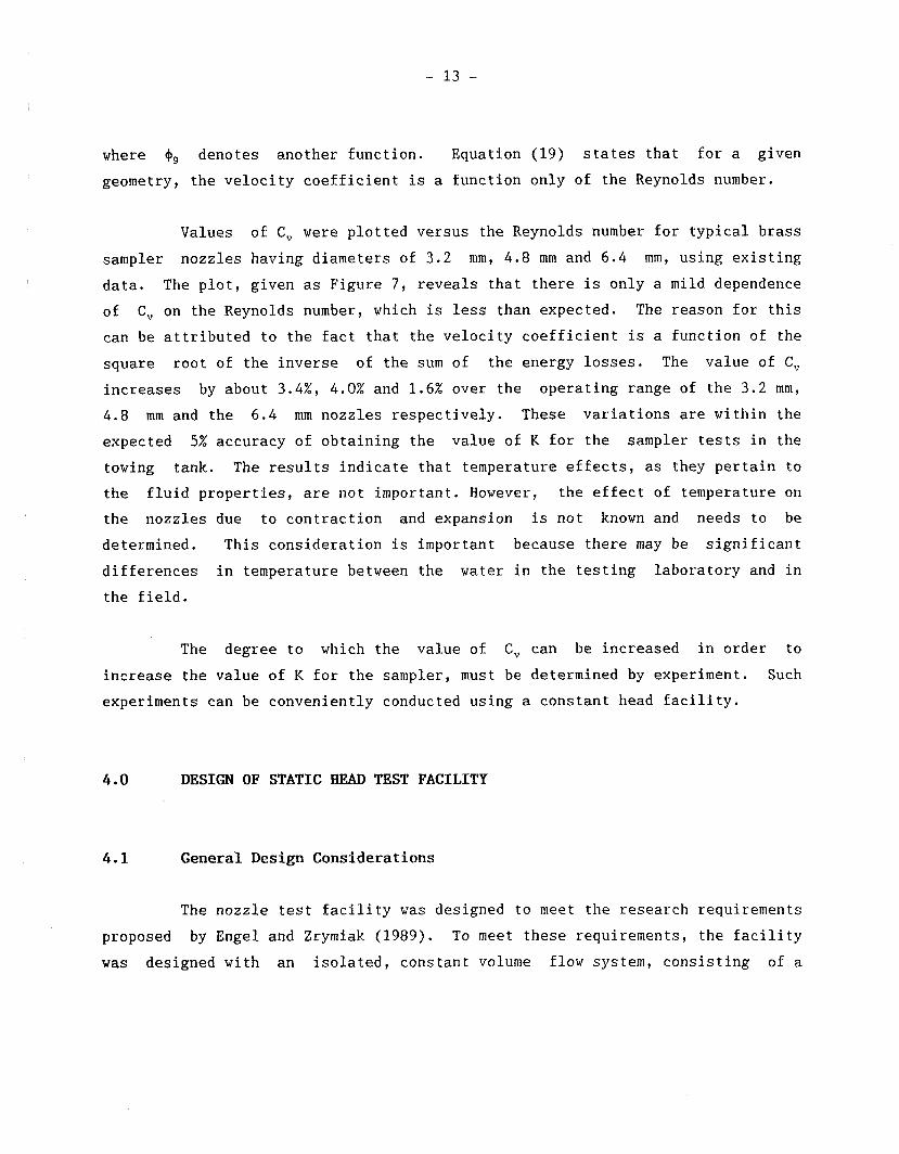
where +9 denotes another function. Equation (19) states that for a given

geometry, the velocity coefficient is a function only of the Reynolds number.

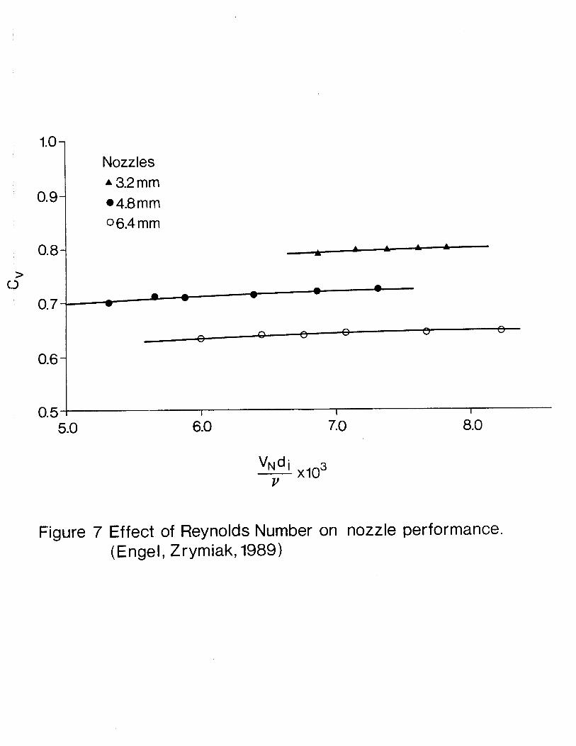
Values of C, were plotted versus the Reynolds number for typical brass

sampler nozzles having diameters of 3.2 mm, 4.8 mm and 6.4 mm, using existing

data. The plot, given as Figure 7, reveals that there is only a mild dependence

of C, on the Reynolds number, which is less than expected, The reason for this

can be attributed to the fact that the velocity coefficient is a function of the

square root of the inverse of the sum of the energy losses. The value of C,

increases by about 3.4%, 4.0% and 1.6% over the operating range of the 3.2 mm,

4.8 mm and the 6.4 mm nozzles respectively. These variations are within the

expected 5% accuracy of obtaining the value of K for the sampler tests in the

towing tank. The results indicate that temperature effects, as they pertain to

the fluid properties, are not important. However, the effect of temperature on

the nozzles due to contraction and expansion is not known and needs to be

determined. This consideration is important because there may be significant

differences in temperature between the water in the testing laboratory and in

the field.

The degree to which the value of C, can be increased in order to

increase the value of K for the sampler, must be determined by experiment. Such

experiments can be conveniently conducted using a constant head facility.

4.0 DESIGN OP STATIC HEAD TEST FACILITY

General Design Considerations

The nozzle test facility was designed to meet the research requirements

proposed by Engel and Zrymiak (1989). To meet these requirements, the facility

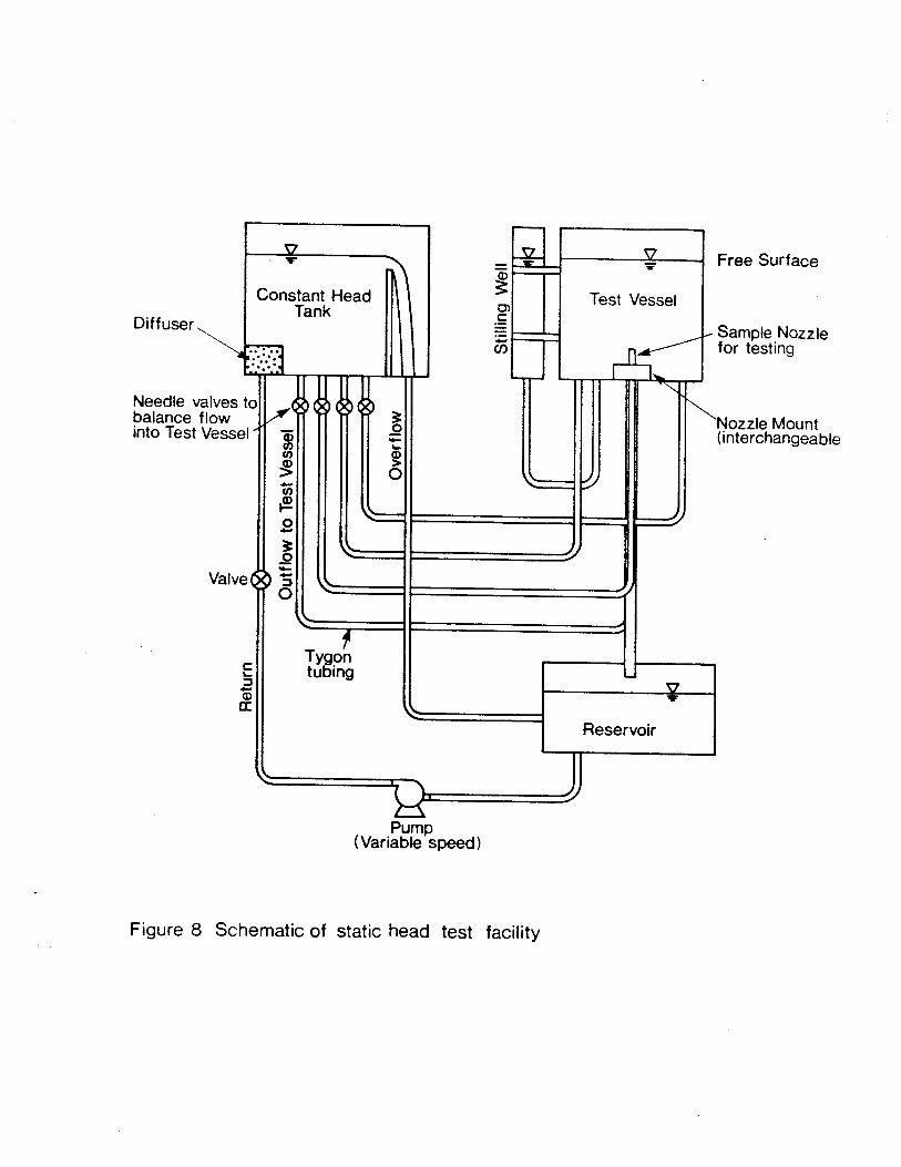
was designed with an isolated, constant volume flow system, consisting of a

fluid reservoir, a constant head tank and the nozzle test chamber. The vertical

position of the latter can be changed to vary the static head on the nozzles.

The main features of the design are shown schematically in Figure 8.

4.2 The Nozzle Test Chamber

Consistent and repeatable testing of the sampler nozzles requires

steady and uniform flow conditions in the nozzle test chamber. To accomplish

this, a cylindrical test chamber, isolated from the constant head tank was

chosen. The test chamber has an inside diameter of 40 cm (16 in.) and a height

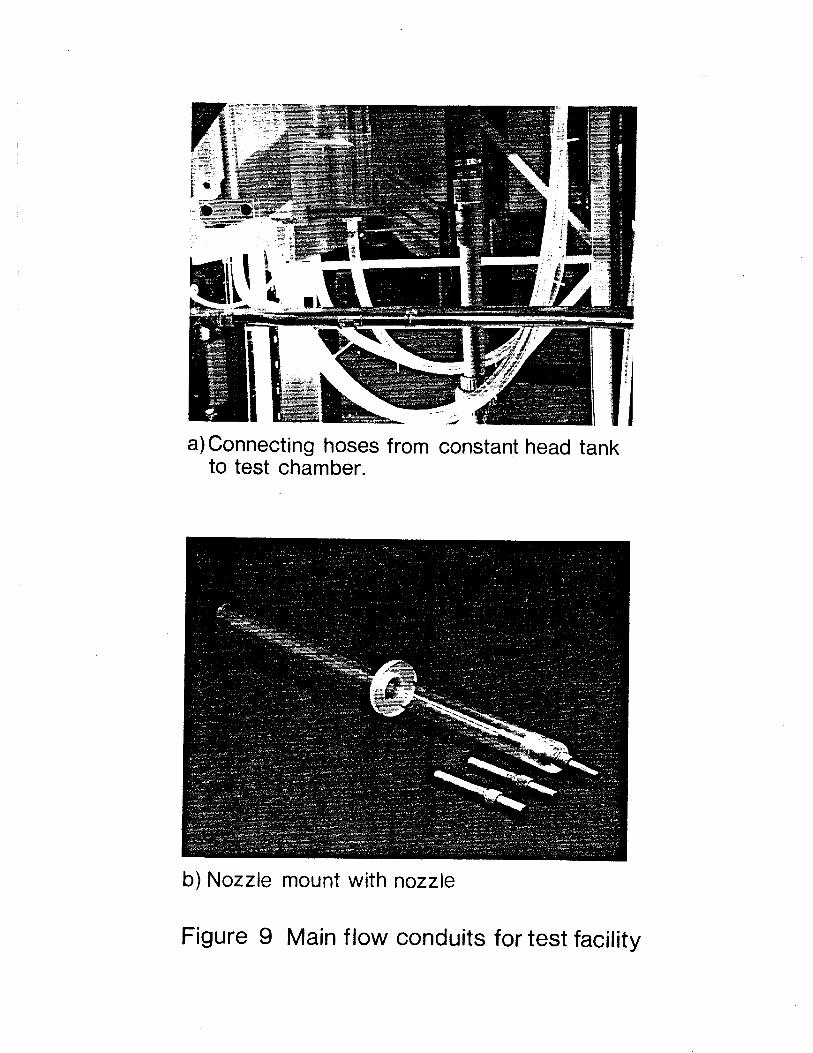
of 95 cm (37.5 in.). Flow from the constant head tank to the test chamber is

passed through four 1.9 cm ( 3 / 4 in.) inside diameter hoses connected to the base

of the chamber as shown in Figure 9 (a). The use of four hoses of the given size

and the chosen location of connection with the test chamber ensures that the

inflow velocities at the base of the test chamber are small. As a result there

are no significant flow circulations set up.

Each test nozzle is fastened to a detachable mount which serves

simultaneously as the outflow conduit as shown in Figure 9(b). The nozzle mount

was fabricated from acrylic to permit observation of the flow as it leaves the

nozzles. The nozzle is placed in the proper test location by passing the nozzle

mount through the hole in the centre of the base of the test chamber and

securing it at a predetermined elevation. The vertical, concentric alignment of

the nozzle and the outflow conduit ensures that the flow through the nozzle will

be uniformly distributed for all anticipated test conditions. Further, to

ensure that there will be no adverse flow circulations when water levels in the

test chamber are near the minimum, a circular baffle, concentric with the

centreline of the nozzle, has been included in the design.

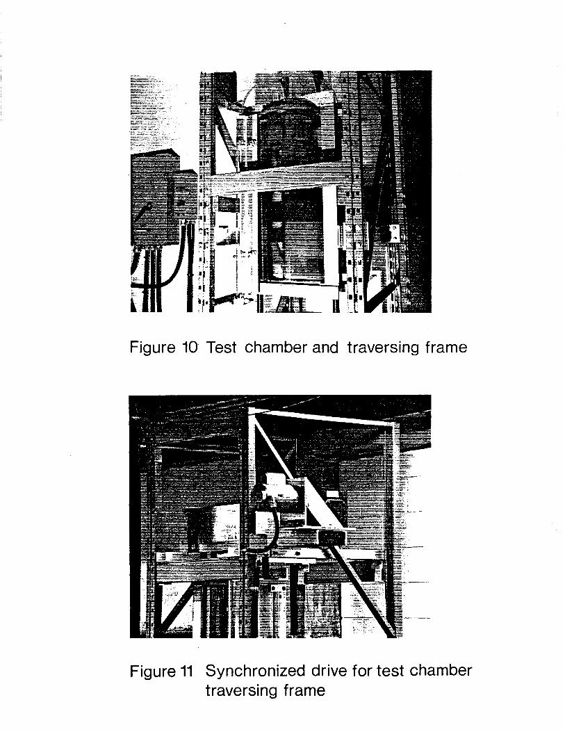
The water level in the test chamber is changed by vertical movement of

the test chamber. To accomplish this, the test chamber is fastened into a

vertical traversing frame as shown in Figure 10. The traversing frame permits

the test chamber to travel over a vertical distance of about 75 cm. The

movement of the frame is accomplished with two synchronized, power driven screw

jacks fastened to the top of the main frame of the test facility as shown in

Figure 11. This drive system permits very precise positioning of the test

chamber,

4 . 3 Constant Head Tank

During each test the water level in the test chamber is maintained at a

constant and steady level because the water is supplied by the constant head

tank. Water is pumped from the reservoir at the base of the test facilty using

a low head, magnetic drive pump. The performance curve for the pump is given in

Figure 12. The capacity of the pump exceeds the maximum discharge required for

the nozzle tests.

The tank is partitioned into two parts by a weir plate, thus creating a

constant head compartment on the upstream side of the weir plate and an overflow

compartment on the downstream side. The water enters the constant head

compartment from the pump through a diffuser which reduces undesirable

turbulence set up by the inflow jet. As the water is pumped into the constant

head tank, the water level rises until the crest elevation of the weir plate has

been reached. Thereafter the water will begin to flow over the crest into the

overflow compartment. The water level in the constant head compartment will

continue to rise until the head required to pass the overflow over the weir

plate has been reached. The overflow drains through a discharge pipe back into

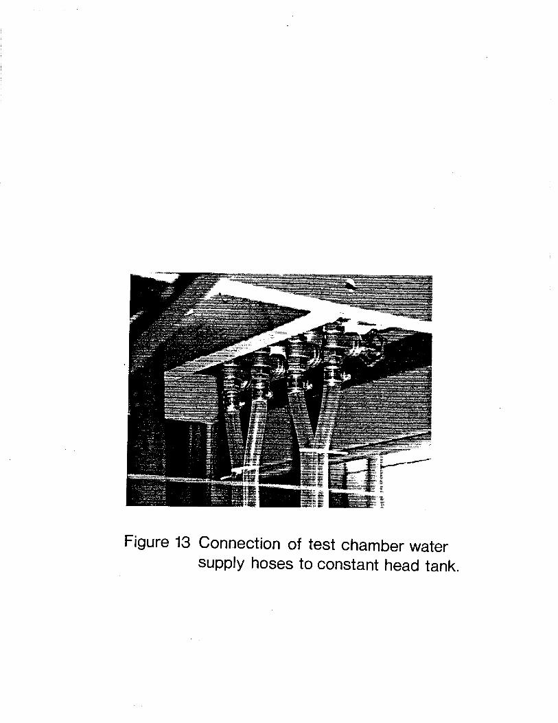
the pumping reservoir. The constant head compartment is connected to the nozzle

test chamber by four 1.9 cm ( 3 / 4 in.) inside diameter hoses, described in

Section 4.2, placed parallel to the weir plate as shown in Figure 13.

4.4 Stilling Well

Water levels in the nozzle test chamber are measured using a graduated

scale, with a resolution of 0.5 mm, mounted on a 5 cm (2 in.) inside diameter

stilling well as shown in Figure 14. The stilling well is mounted on the

traversing frame of the test chamber and is connected to the water column in the

test chamber with a 1 cm (3/8 in.) inside diameter plastic tube at the base

inside the cylindrical baffle.

5.0 PRELIMINARY TESTS

Tests were conducted, using brass nozzles compatible with the DH48

suspended sediment sampler. These tests were intended to establish the

variability in the determination of the velocity coefficients at different

static heads over the operating range of the test facility.

T e s t P r o c e d u r e

Each sediment sampler is equipped with three sizes of nozzles,

having inside diameters of 3.2 mm (1/8 in.), 4.8 mm (3/16 in.) and 6.4 mm ( 1 / 4

in.), each size being applicable to a particular range of velocities. The three

nozzles are shown in Figure 15.

Prior to testing, a nozzle was selected, its length measured and

fastened to the nozzle mount which was then secured in the base of the test

chamber as described in Section 4.2 and shown in Figure 16. The outflow end of

the nozzle mount was then sealed with a rubber plug provided for this purpose

and the pump was turned on. As the water entered the constant head tank, it

flowed immediately through the plastic hoses into the test chamber. The water

was allowed to rise in the test chamber until the mouth of the nozzle was

covered by several millimeters of water. The pump was then turned off and the

stopper removed from the nozzle mount, The water drained through the nozzle

mount into the reservoir until the water surface was level with the mouth of the

nozzle. This water level was noted on the graduated scale along the stilling

well and taken as the reference datum during the tests for this nozzle.

Once the preliminary procedures were completed, the rubber plug was

replaced in the outflow end of the nozzle mount, the pump was turned on and the

test chamber was positioned for the first test. Initially, as the water entered

the constant head tank, all of the water flowed directly into the test chamber.

As the water level in the test chamber rose, the difference in water elevation

between the constant head tank and the test chamber decreased and the rate of

increase in water level in the test chamber decreased. When the water level in

the constant head tank and the test chamber were equal, all flow into the test

chamber ceased and the total pumped flow was passed through the overflow

compartment of the constant head tank into the reservoir. At this time the

rubber plug was removed from the nozzle mount to allow flow to pass through the

nozzle into the water reservoir. Once again the water levels underwent a change

until the difference between the water surface elevations in the constant head

tank and the test chamber were equal to the head required to supply the

discharge passing through the nozzle. When this steady state was reached, the

required measurements were made.

The following measurements were carried out: the water level elevation

in the test chamber stilling well relative to the reference datum, the volume of

water discharged through the nozzle and the time required to pass that volume of

water. The volume of water was measured using a 1 litre graduated cylinder. For

each value of static head, the discharge was measured by intercepting the

outflow jet from the nozzle with the graduated cylinder and simultaneously

starting the quartz crystal stop watch. When the cylinder was nearly full (ie:

about 950 c.c.), it was quickly withdrawn and the stop watch simultaneously

stopped. Care was taken that the volume of water was always near 950 C.C. to

ensure that errors in its measurement as well as in the corresponding time were

sufficiently small. Using these measurements the theoretical velocity and the

actual velocity of the flow passing through the nozzle were computed. Tests

were conducted for each nozzle at about ten different heads from about 1 cm to

65 cm. For each value of the head, measurements of water levels, volume of

discharge and time were made 10 times in order to obtain a sufficiently large

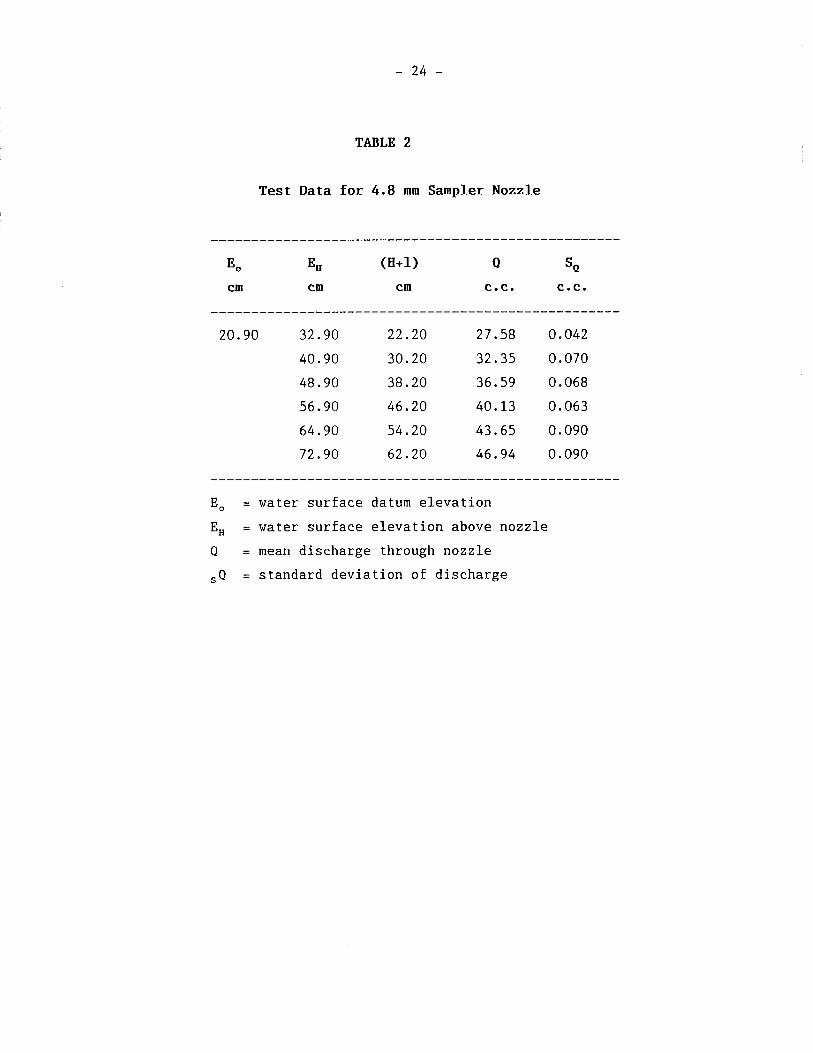
set of data for statistical analysis. The test data are given in Tables 1 for

the 3.2 mm nozzle, Table 2 for the 4.8 mm nozzle and Table 3 for the 6.4 mm

nozzle.

5.2 Data Analysis

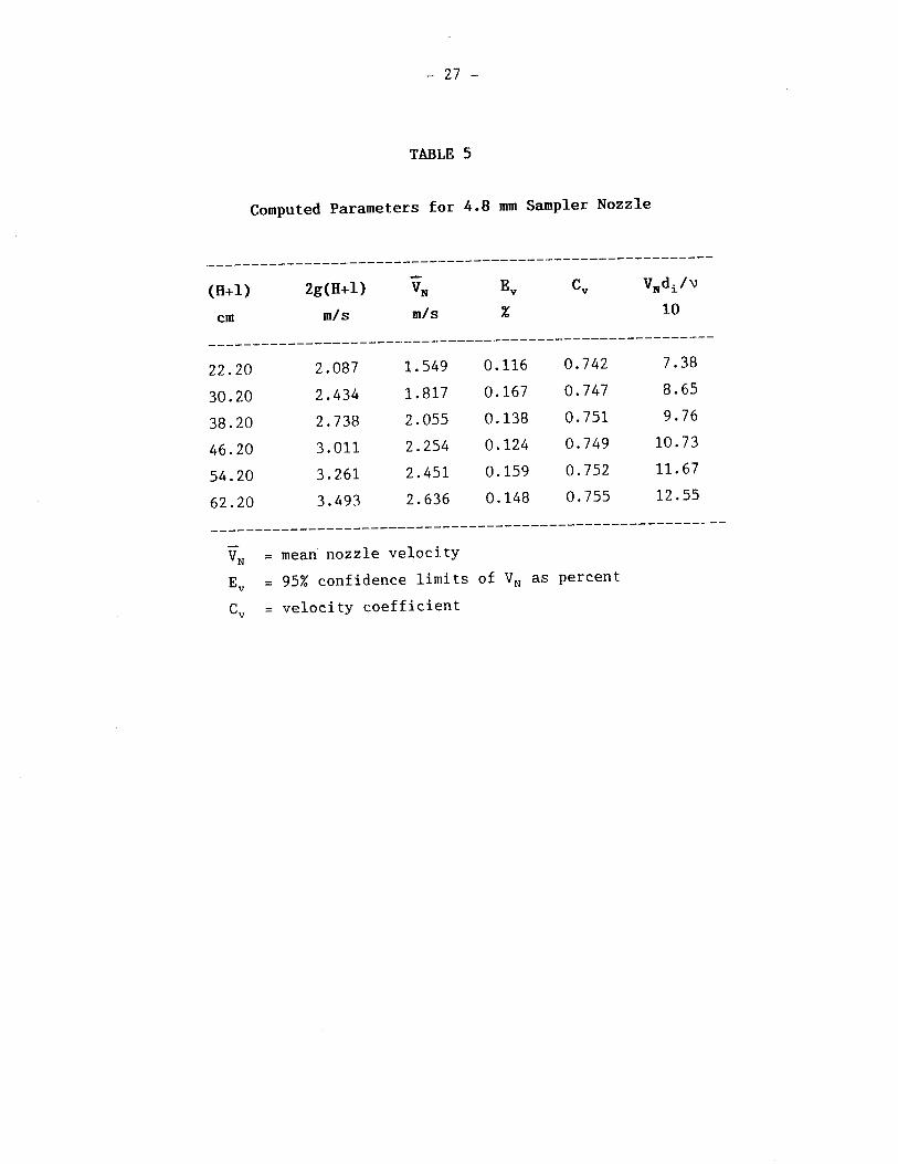
The data in Tables 1,2 and 3 were used to compute the ideal nozzle

velocity according to equation (2) and the actual nozzle velocity by dividing

the discharge Q by the cross sectional area of the nozzle flow passage. Using

these velocities, the coefficient C, was computed from equation (3) together

with the corresponding Reynolds numbers. These results are given in Tables 4,5

and 6 for the 3.2 mm, 4.8 mm and the 6.4 mm nozzles respectively.

Any one of the 10 nozzle velocity samples of magnitude V, used to

compute the mean for each flow condition can be expected to lie within the range

- where V, = the value of a single velocity sample measured, V, = the mean of all

the measured velocities at a given head, t, = the confidence coefficient from

Student's "t" distribution at nine dgrees of freedom (Spiegel, 1961) and S, =

the standard deviation about the mean velocity. Equation (20) can be made

dimensionless by dividing both sides by the mean V,. In addition, since the

coefficient of variation, say, C = S,/V,, one obtains

The product t,C in equation ( 21 ) represents the relative variability of the

velocity samples and is expressed as

where E, is the relative variability of the velocity samples in percent, Values

of E, at the 95% confidence level were computed and are given in Table 4,5 and 6

for the 3.2 mm, 4,8 mm and 6.4 mm nozzles, respectively.

Values of E, are plotted as a function of the mean velocities for the

three nozzles in Figure 17. The data show that values of E, for each nozzle

are at most only mildly dependent on the magnitude of the nozzle velocity. It

can also be seen from Figure 17 that the variability tends to increase as the

size of the nozzle increases. The reason for this is that the volume of water

which is collected to determine the discharge through the nozzles increases with

the diameter of the nozzles. Measurements were made with a graduated cylinder

having a 1 litre capacity. As the discharge increases, the cylinder fills up

more quickly, thus increasing the error in the measurement of the time required

to collect the volume of water. Obviously, the variability can be reduced by

increasing the volume of water and thereby increasing the length of measuring

time. However, the variability with the present method is less than 0.3% and

this is sufficiently small, so that no changes in the test method are required.

Values of the velocity coefficient C, for each size of nozzle were

plotted as a function of the Reynolds number in Figure 18. Smooth average

curves, fitted by eye, were drawn through the plotted data to facilitate easier

comparison of the characteristics of the three nozzles. The curves exhibit the

same ,trend of mild dependence of C, on the Reynolds number as the curves in

Figure 7. However, for a given value of the Reynolds number, values of C, in

Figure 18 are always a little larger than those in Figure 7, eventhough both

Figures represent nozzles of the same type. The reason for this is that each

set of nozzles has been adjusted to match a particular sediment sampler in order

to obtain a value of K within 10% of the sought after value of 1.0. This is

further proof that very small changes to the nozzles can result in significant

changes in their performance.

6.0 CONCLUSIONS

6.1 Each suspended sediment sampler must be tested to ensure

that it operates iso-kinetically. If tests in the towing tank indicate

that the performance of the sampler deviates from iso-kinetic behaviour

by more than 5%, then adjustments must be made. Experience has shown

that such adjustments can be made either to the sampler body itself,

the nozzles or both, depending on the degree of adjustment required.

Adjustment to the sampler bodies can be made by changing the air

exhaust conduit and the air exhaust port to increase or decrease the

resistance to the air outflow as required. Adjustments to the nozzles

can be made by decreasing the hydraulic resistance and thus increasing

the discharge through the nozzle which in turn increases the flow

velocity through the nozzle.

Analysis indicates that small changes in boundary roughness of the flow

passage in the nozzles has virtually no effect on the friction factor

for the nozzles. This is due to the fact that the flow through the

brass nozzles is in the smooth turbulent flow regime. For the Reynolds

numbers in the operating range of the brass nozzles, the friction

factor varies from 0.038 to 0.031. Similar results can be expected for

plastic nozzles.

6.4 Evidence has been obtained to indicate that small changes in the nozzle

outlet geometry will result in significant reduction in energy losses

with resultant increase in discharge and flow velocity through the

nozzles.

6.5 The coefficient of velocity was found to vary mildly with the Reynolds

number. Therefore, temperature effects on the performance of the

nozzles as far as fluid properties are concerned will be minor.

However, effects of water temperature on the material nozzle properties

such as shrinking and expansion need to be examined.

For a given Reynolds number, the coefficient of velocity was found to

increase as the diameter of the nozzles decreased. These results were

obtained with typical brass nozzles but can be expected to be similar

for plastic nozzles.

6.7 Tests with the static head facility have shown that determinations of

nozzle flow velocities have a variability of less than 0.3% at the 95%

confidence level. Therefore, the static head facility will be

satisfactory for the calibration of suspended sediment sampler nozzles.

The static head facility was fabricated by G. Voros and K. Davies. The

nozzle tests were conducted by C. Bil and all photographs were provided by D.

Doede. The writer is very grateful for their dedicated efforts on this project.

The writer is indebted to P. Zrymiak of the Sediment Survey Section, Water

Survey of Canada for his careful review of the manuscript.