management strategy evaluation (mse) of the harvest...
TRANSCRIPT

Management strategy evaluation (MSE) of the harvest strategy
for the Small Pelagic Fishery
F. Giannini, P.I. Hobsbawn, G.A. Begg, M. Chambers
FRDC Project 2008/064

FRDC Project 2008/064 ii
Management strategy evaluation (MSE) of the harvest strategy for the Small Pelagic Fishery, F. Giannini, P.I. Hobsbawn, G.A. Begg, M. Chambers, May 2010, Bureau of Rural Sciences. © Copyright Fisheries Research and Development Corporation and Bureau of Rural Sciences 2010
This work is copyright. Except as permitted under the Copyright Act 1968 (Cth), no part of this publication may be reproduced by any process, electronic or otherwise, without the specific written permission of the copyright owners. Information may not be stored electronically in any form whatsoever without such permission. Disclaimer The authors do not warrant that the information in this document is free from errors or omissions. The authors do not accept any form of liability, be it contractual, tortious, or otherwise, for the contents of this document or for any consequences arising from its use or any reliance placed upon it. The information, opinions and advice contained in this document may not relate, or be relevant, to a readers particular circumstances. Opinions expressed by the authors are the individual opinions expressed by those persons and are not necessarily those of the publisher, research provider or the FRDC. The Fisheries Research and Development Corporation plans, invests in and manages fisheries research and development throughout Australia. It is a statutory authority within the portfolio of the federal Minister for Agriculture, Fisheries and Forestry, jointly funded by the Australian Government and the fishing industry. ISBN 978-1-921192-50-0

FRDC Project 2008/064 iii
Contents
Non-technical summary .................................................................................................................1 Acknowledgements ........................................................................................................................4
1. Introduction................................................................................................................................5 1.1. Background.............................................................................................................................5 1.2. Fishery ....................................................................................................................................5 1.3. Need .......................................................................................................................................7 1.4. Objectives...............................................................................................................................7
2. Data inputs .................................................................................................................................8 2.1. Introduction.............................................................................................................................8
2.1.1. Redbait............................................................................................................................8 2.1.2. Blue mackerel ...............................................................................................................12 2.1.3. Jack mackerel ...............................................................................................................15 2.1.4. Australian sardine (east) ...............................................................................................18 2.1.5. Australian sardine (west) – Test case...........................................................................21
3. Management Strategy Evaluation (MSE)...............................................................................24 3.1. Introduction...........................................................................................................................24 3.2. Model description .................................................................................................................25
3.2.1. Population dynamics.....................................................................................................25 3.2.2. Stock-recruitment..........................................................................................................26 3.2.3. Spawning biomass........................................................................................................30 3.2.4. Catches.........................................................................................................................30
3.3. Implementation of the harvest strategy in the model ...........................................................32 3.4. Performance statistics ..........................................................................................................33 3.5. MSE scenarios .....................................................................................................................34 3.6. Test case: Australian sardine (west) ....................................................................................37 3.7. Results..................................................................................................................................38
3.7.1. Base case scenarios.....................................................................................................38 3.7.2. Sensitivity analysis........................................................................................................38 3.7.3. Australian sardine (west) – test case............................................................................40
3.8. Discussion ............................................................................................................................41 4. Research Plan ..........................................................................................................................45
4.1. Introduction...........................................................................................................................45 4.2. Current and past monitoring.................................................................................................45 4.3. Research and monitoring requirements ...............................................................................46
4.3.1. Tier 1 data requirements...............................................................................................46 4.3.2. Tier 2 data requirements...............................................................................................47

FRDC Project 2008/064 iv
4.3.3. Tier 3 data requirements...............................................................................................48 4.4. Discussion ............................................................................................................................48
5. Discussion................................................................................................................................51 6. Benefits and adoption.............................................................................................................53 7. Further development ...............................................................................................................54 8. Planned outcomes...................................................................................................................55 9. Conclusion ...............................................................................................................................56 10. References ...............................................................................................................................57 Appendix A. Intellectual property..................................................................................................59 Appendix B. Staff ............................................................................................................................60 Appendix C. Small Pelagic Fishery Harvest Strategy (June 2008).............................................61 Appendix D. MSE code ...................................................................................................................70 Appendix E. MSE sensitivity analysis........................................................................................ 102
Redbait A (east) ........................................................................................................................ 102 Redbait B (west)........................................................................................................................ 109 Blue mackerel A (east) .............................................................................................................. 115 Blue mackerel B (west) ............................................................................................................. 122 Jack mackerel ........................................................................................................................... 129 Australian sardine (east) ........................................................................................................... 135 Test case: Australian sardine (west) SA ................................................................................... 142
Appendix F. MSE workshop minutes ......................................................................................... 148 Appendix G. Case study of sample design to estimate proportion of catch-at-age for
redbait ...................................................................................................................................... 152 Example .................................................................................................................................... 154 Recommended sample design: one-stage sampling ................................................................ 156 Data collection........................................................................................................................... 156

FRDC Project 2008/064 1
Non-technical summary Project title: Management strategy evaluation (MSE) of the harvest strategy for the Small
Pelagic Fishery FRDC project number: 2008/064 Principal investigator: Patricia I. Hobsbawn Address: Fisheries and Marine Sciences Program Bureau of Rural Sciences Department of Agriculture, Fisheries and Forestry GPO Box 858 Canberra ACT 2001 Telephone: 02 6272 3933 Objectives: 1. Develop and implement an appropriate management strategy evaluation (MSE) to aid the
review of the Small Pelagic Fishery (SPF) Harvest Strategy. 2. Use the MSE to investigate the harvest strategy’s performance under a range of plausible
scenarios. 3. Develop a research plan, including indicative costs, to collect the data required for the harvest
strategy (all Tiers) to meet its objectives. Non-technical summary Outcomes achieved to date: A new management strategy evaluation (MSE) tool has been developed for the Small Pelagic Fishery (SPF). The sensitivities of this operating model have been tested and various harvest strategies explored, as outlined in the SPF Harvest Strategy as well as alternatives to these. A research plan has been developed to underpin the SPF Harvest Strategy and is already being implemented. In 2008, the Australian Fisheries Management Authority (AFMA) developed a harvest strategy for the Commonwealth’s Small Pelagic Fishery (SPF) (AFMA 2008) in accordance with the Commonwealth Fisheries Harvest Strategy Policy (DAFF 2007). Before its completion, an independent review was conducted (Knuckey et al. 2008), which included a management strategy evaluation (MSE). The equations developed for the MSE were used in this report to establish a new MSE. The new MSE was used to further test the SPF Harvest Strategy and to investigate a range of alternative harvest strategies for consideration by the Small Pelagic Fisheries Resource Assessment Group (SPFRAG). In this report, the sensitivities of the MSE were tested to determine how the various input parameters influenced the outcomes over a 30 year simulation period. A number of management/harvest scenarios were run through the MSE to explore options addressed in the SPF Harvest Strategy for each stock — redbait (east), redbait (west), blue mackerel (east), blue mackerel (west), jack mackerel (east and west treated the same) and Australian sardine (east). The
FRDC Project 2008/064 2
model was found to be most sensitive to the steepness value in the stock-recruitment relationship and to the value of the instantaneous natural mortality. The current SPF Harvest Strategy has a three-tiered approach. At the Tier 1 level, the maximum recommended biological catch (RBC) for each stock depends on the time since a daily egg production method (DEPM) survey was conducted, with the maximum RBC decaying from 20 percent to 10 percent of the spawning biomass estimated from the DEPM survey over a five year period (relative tonnage). The maximum RBC for Tier 2 and Tier 3 is set at a specified quantity (absolute tonnage). A maximum RBC for Tier 2 has been defined for each stock with quantities varying from 3000-6000 tonnes, while for Tier 3, the maximum RBC has been set at 500 tonnes for each stock. The Tier 1 base case used in the MSE in this project assumed a DEPM survey was conducted once every five years, however, a scenario involving a DEPM survey once every two years was also investigated. Alternative Tier 1 harvest strategies to those identified in the SPF Harvest Strategy were also investigated. In particular, using a constant 15 percent harvest rate as one scenario and a constant 7.5 percent harvest rate as another scenario in the five years between DEPM surveys, as opposed to the decay from 20 percent to 10 percent over the five years. In most management/harvest scenarios, the 30 year simulation period used in the MSE was sufficient for each stock to reach equilibrium, and generally this was well above 20 per cent of virgin biomass levels (B20). The results of Tier 2 and Tier 3 harvest strategies show that tonnages for each stock are most likely conservative and sustainable. However, these results need to be treated with caution as these absolute tonnages represent a much smaller proportion of the larger model derived biomasses than those biomasses determined by the DEPM surveys. The code for the MSE is being made available to the SPFRAG. It can then be used to further explore alternative harvest strategies and management options. Since the 2008/09 fishing season, RBCs have been set using Tier 1 rules for stocks where a DEPM survey has been conducted, and using Tier 2 rules where there has been no spawning biomass estimate. The SPF is currently moving towards a Tier 2 fishery for all stocks and thus the research plan developed through the current project indicates that the highest priorities for research are:
1. an annual fishery assessment report 2. the design and conduct of an appropriate monitoring program.
The research plan is currently being implemented with a project led by the South Australian Research and Development Institute (SARDI) in collaboration with the Tasmanian Aquaculture and Fisheries Institute (TAFI) and the Bureau of Rural Sciences (BRS). It will produce a fishery assessment report and collate information on age/size structure of the target stocks, and outcomes will enable the minimum requirements for Tier 2 assessments to be met. In conclusion, the results produced in this study show that Tier 1 harvest strategies, using proportions of the spawning biomass to determine RBCs, are most likely sustainable and well above B20. Results for Tier 2 and Tier 3 harvest strategies should be treated with caution as these use absolute tonnages for harvest quantities that may not be meaningful for the model calculated

FRDC Project 2008/064 3
spawning biomass estimates. Future work should examine potential discrepancies between the model calculated virgin spawning biomasses and those derived from the DEPM surveys. Keywords: Management strategy evaluation, Small Pelagic Fishery, harvest strategy, redbait, Emmelichthys nitidus, blue mackerel, Scomber australasicus, jack mackerel, Trachurus declivis, Trachurus murphyi, Australian sardine, Sardinops sagax.
FRDC Project 2008/064 4
Acknowledgements The project was funded by the Fisheries Research and Development Corporation (FRDC) and the Bureau of Rural Sciences (BRS) Division, within the Department of Agriculture, Fisheries and Forestry (DAFF). This research was supported by the Reducing Uncertainty in Stock Status (RUSS) project, under the Commonwealth government’s expanded Fisheries Research Program. Data were received from the South Australian Research and Development Institute (SARDI) (Tim Ward), Tasmanian Aquaculture and Fisheries Institute (TAFI) (Jeremy Lyle and Andrew Browne) and New South Wales Department of Primary Industries (NSWDPI) (John Stewart). Invaluable assistance, advice and support were received from Tim Ward (SARDI), Jeremy Lyle (TAFI), Dennis Brown (industry), Phil Domaschenz, Selina Stoute from the Australian Fisheries Management Organisation (AFMA), and members of the Small Pelagic Fishery Resource Assessment Group and Management Advisory Committee. Michael O’Neill from the Queensland Department of Primary Industries and Fisheries (QDPI&F) provided initial advice on the management strategy evaluation as part of an independent review of the project. Malcolm Haddon from the Commonwealth Scientific and Industrial Research Organisation (CSIRO) also provided an independent review.

FRDC Project 2008/064 5
1. Introduction
1.1. Background Commonwealth fisheries are required to implement harvest strategies to guide their management in accordance with the Commonwealth Fisheries Harvest Strategy: Policy and Guidelines (DAFF 2007). Harvest strategies provide agreed processes for monitoring and assessment, reference points, indicators and control rules for managing a fishery so that it meets specific objectives. However, the reality is that fisheries are characterised by considerable uncertainty and variability. Fishing activities fluctuate with the availability of fish, markets and weather conditions; there is considerable uncertainty over stock abundance indices and biological parameters, including age structure, natural mortality, stock-recruitment, age-at-maturity and stock structure; and environmental variations and ecological factors also have a pervading influence. It is necessary, therefore, to demonstrate that a proposed harvest strategy will meet its fishery objectives over a wide range of management/harvest scenarios. The Commonwealth Fisheries Harvest Strategy Policy (HSP) recommends the application of a management strategy evaluation (MSE) to test how robust harvest strategies are to different management scenarios and control rules. In June 2008, the Australian Fisheries Management Authority (AFMA) Board approved the Commonwealth Small Pelagic Fishery (SPF) Harvest Strategy (AFMA 2008; see Appendix C). The harvest strategy is a three tier strategy reflecting variable levels of data and concomitant levels of harvest with a recommended biological catch (RBC) for each species determined by the level of assessment conducted. The RBC differs from the Total Allowable Catch (TAC) because catches from other jurisdictions need to be considered in the assessment. A Tier 3 assessment (the lowest level and most data poor assessment) in the SPF Harvest Strategy is made when only catch and effort data are available. A Tier 2 assessment is made when catch and effort data are available, together with appropriately sampled age data. A Tier 1 assessment (the most robust and data rich assessment) is made when a daily egg production method (DEPM) survey has been conducted and the recommended RBC is set depending on time since the last DEPM survey. Assessments at each tier are determined by the data gathering and research available for each stock, which underpins the harvest strategy and are identified in an annual research plan. In 2007, a consultant was hired to review the then draft SPF Harvest Strategy (Knuckey et al. 2008). This consisted of a qualitative and quantitative (MSE) component. The SPF Resource Assessment Group (SPFRAG) found the results of the MSE insightful and wished to use the technique to explore further management scenarios related to RBCs. The equations used to develop the MSE were provided in the final report of the review (Knuckey et al. 2008), however, the model code used to produce the results was not made available to the SPFRAG. The main aim of this project was to evaluate the MSE approach used in the Knuckey et al. (2008) review and to develop model code with which to run alternative scenarios and be available to the SPFRAG for further consideration. The project also aimed to scope the initial annual research plan required to provide data and assessments to underpin the harvest strategy for the SPF.
1.2. Fishery The SPF covers that part of the Australian Fishing Zone (AFZ) along the south coast of Australia and around Tasmania. It extends from the New South Wales/Queensland border in the east to Lancelin, north of Perth, in the west. Historically, this area has been divided into four management zones as shown in Figure 1.1. Since the introduction of the SPF Harvest Strategy in 2008, stocks in

FRDC Project 2008/064 6
the fishery are now managed along an east/west divide. For the setting of the 2008/09 RBCs, the east/west divide was taken as 146º30’E (AFMA 2008b).
Figure 1.1: The Small Pelagic Fishery with the new east/west divide at 146°30’ longitude and the old management zones (A, B, C, D).
There are four target species in the SPF: redbait (Emmelichthys nitidus); blue mackerel (Scomber australasicus); jack mackerels (Trachurus declivis, T. murphyi); and Australian sardine (Sardinops sagax). Yellowtail scad (Trachurus novaezelandiae) is managed as a byproduct species. The first three of these species are divided into eastern and western stocks; for Australian sardine, the SPF has jurisdiction only in Commonwealth waters off the coast of New South Wales and part of Queensland. The permitted fishing methods for targeting these species in the fishery are purse-seining and mid-water trawling. Historically, most catches in the SPF have been jack mackerel purse-seined in Zone A within three nautical miles of eastern Tasmania. The fishery developed rapidly from an annual catch of 6000 t in 1984/85 to a peak of almost 42 000 t in 1986/87. Catches during the next decade were between 8000 t and 32 000 t. Catches have declined significantly since that time. In 2003 and 2004, increased catches mainly comprised redbait (Hobsbawn and Summerson, 2008). Species targeted in the SPF are also taken in several other Commonwealth- and state-managed fisheries, mainly the trawl sectors of the Southern and Eastern Scalefish and Shark Fishery (SESSF); the Eastern Tuna and Billfish Fishery (ETBF) and the Western Tuna and Billfish Fishery (WTBF) (where they are purse-seined for bait); and the New South Wales Ocean Hauling Fishery (Hobsbawn and Summerson, 2008).

FRDC Project 2008/064 7
1.3. Need Commonwealth fisheries have been required to implement harvest strategies in accordance with the recently released Commonwealth Fisheries Harvest Strategy Policy. The policy requires an MSE be conducted to demonstrate that each harvest strategy is robust to the uncertainty inherent in the assessment and management of the respective fishery. In 2007, AFMA engaged a consultant to review the draft harvest strategy that had been developed for the SPF (Knuckey et al. 2008). Based on the outcomes of that review, which included a quantitative evaluation via an MSE, the SPFRAG and SPF Management Advisory Committee (SPFMAC) agreed to the harvest strategy. In June 2008, the AFMA Board approved the SPF Harvest Strategy. However, further testing of the harvest strategy was required to investigate its robustness under a range of harvest scenarios.
1.4. Objectives 1. Develop and implement an appropriate MSE to aid the review of the SPF Harvest Strategy. 2. Use the MSE to investigate the harvest strategy’s performance under a range of plausible
scenarios. 3. Develop a research plan, including indicative costs, to collect the data required for the
harvest strategy (all tiers) to meet its objectives.

FRDC Project 2008/064 8
2. Data inputs
2.1. Introduction Spawning biomass estimates have been determined in previous studies from DEPM surveys for redbait (east stock) (Neira et al. 2008), blue mackerel (east and west stocks) and Australian sardine (east stock) (Ward and Rogers 2007). These are the only stocks for which actual DEPM data could be used to set the initial conditions for the operating model used in the MSE (see Chapter 3). For all other stocks a simulated population was used for the initial conditions. Where actual data could be used, six parameters were determined to set the initial conditions for the model. These were:
1. initial spawning biomass ( spB0 ) 2. numbers of fish in each age class in the samples from the survey (together with initial
spawning biomass gives numbers of fish in the population, aN ,0 ) 3. mortality in each age class ( aM ) 4. selectivity-at-age ( aS ) 5. average weight-at-age ( aw ) 6. proportion of sexually mature fish-at-age ( af ).
Length and age data were obtained from the Tasmanian Aquaculture and Fisheries Institute (TAFI) for redbait, South Australian Research and Development Institute (SARDI) for blue mackerel and the New South Wales Department of Primary Industries (NSWDPI) for Australian sardine. These unpublished data were used to determine some of the parameters outlined above.
2.1.1. Redbait Data (unpublished) for adult redbait were provided by TAFI (Table 2.1). Age and fork length (FL) were provided for each individual fish, together with region and year of sampling. Separate data sets were compiled for each of the eastern and western stocks. Data from all years were pooled to obtain the frequencies in each age group.
Table 2.1: Number of redbait sampled by year (2003–2006) and stock (east, west). Year East West 2003 165 4 2004 349 178 2005 217 170 2006 70 112
Total 801 464
The length-weight relationship used for redbait (both east and west stocks) was obtained from TAFI (Figure 2.1):

FRDC Project 2008/064 9
3416.3000002.0 FLW = where W is body weight (g) and FL is fork length (mm).
y = 2E-06x3.3416
R2 = 0.9725
0
100
200
300
400
100 150 200 250 300 350
Length (mm)
Wei
ght (
g)
Figure 2.1: Fork length (mm) – weight (g) relationship for redbait (both east and west stocks). Catch curves were used to estimate selectivity (S). The regression line was extrapolated to younger ages where fish were not fully recruited to the fishery to give theoretical estimates of numbers of fish in those age groups. The ratio of the number of fish sampled to the theoretically predicted number of fish provided a measure of the selectivity (FAO, 1998), that is regressionobserved NNS /= . The operating model used in the MSE was also used to estimate proportions of fish in age groups. Two options were used, one where the model was used to estimate proportions before fish are fully recruited to the fishery together with actual proportions after that point (Tables 3.4, 3.5 and 3.6: Astart=Data); and the second is where the model is used to estimate proportions in each age group for the entire population (Table 3.4: Astart=Equilibrium). The equation for the catch curve regression for redbait in the east (pooled across years) is:
6772.53198.0)ln( +−= AN where N is the number of fish and A is the age group (years) (Figure 2.2).
Age (Years)
Nat
ural
Log
arith
m o
f Fre
quen
cy
01
23
45
6
0 2 4 6 8 10 12 14 16 18
Redbait (east)
0 2 4 6 8 10
Age (Years)
Sele
ctiv
ity
0.0
0.1
0.2
0.3
0.4
0.5
0.6
0.7
0.8
0.9
1.0
1.1
1.2
Redbait (east)
Figure 2.2: Catch curve and selectivity curve for redbait (east).

FRDC Project 2008/064 10
The equation for the catch curve regression for redbait in the west (pooled across years) is: 2295.52889.0)ln( +−= AN
where N is the number of fish and A is the age group (years) (Figure 2.3).
Age (Years)
Nat
ural
Log
arith
m o
f Fre
quen
cy
01
23
45
6
0 3 6 9 12 15 18 21
Redbait (west)
0 2 4 6 8 10
Age (Years)
Sele
ctiv
ity
0.0
0.1
0.2
0.3
0.4
0.5
0.6
0.7
0.8
0.9
1.0
1.1
1.2
Redbait (west)
Figure 2.3: Catch curve and selectivity curve for redbait (west). Hoenig’s (1983) equation was used to determine natural mortality ( M ) for redbait (both east and west stocks):
)log(982.044.1 AgeMaximumeM −= where AgeMaximum for redbait is 21 years. The proportion of sexually mature fish-at-age, af , was obtained from Knuckey et al. (2008). Table 2.2 provides the input data for redbait (east) used in the MSE operating model (see Chapter 3) as specified above. The spawning biomass estimate for redbait (east) in 2006 from the DEPM was 86 990 tonnes (Neira et al. 2008). Table 2.3 provides the input data for redbait (west) used in the MSE operating model (see Chapter 3) as specified above. There was no spawning biomass estimate from DEPM surveys for redbait (west).

Table 2.2: Input data for redbait (east) used in the MSE operating model.
Age Sample
Frequency Catch Curve Frequency
aN ,0 – DataProportions
aN ,0 – EquilibriumProportions
aM – Natural Mortality
aS Selectivity
aw Weight
af – Proportion of Sexually Mature Fish
0 115 292 0.189 0.189 0.21 0.39 19.64 0.00 1 140 212 0.154 0.154 0.21 0.66 34.50 0.10 2 121 154 0.124 0.124 0.21 0.79 80.62 0.30 3 90 112 0.113 0.101 0.21 1.00 94.56 0.55 4 92 81 0.115 0.082 0.21 1.00 121.71 0.75 5 97 59 0.122 0.066 0.21 1.00 166.78 0.90 6 47 43 0.059 0.054 0.21 1.00 208.14 1.00 7 19 31 0.024 0.044 0.21 1.00 218.47 1.00 8 15 23 0.019 0.035 0.21 1.00 227.38 1.00 9 20 16 0.025 0.029 0.21 1.00 254.77 1.00
10+ 45 40 0.056 0.122 0.21 1.00 291.77 1.00
Table 2.3: Input data for redbait (west) used in the MSE operating model.
Age Sample
Frequency Catch Curve Frequency
aN ,0 – DataProportions
aN ,0 – EquilibriumProportions
aM – Natural Mortality
aS Selectivity
aw Weight
af – Proportion of Sexually Mature Fish
0 0 263 0.189 0.189 0.21 0.00 58.05 0.00 1 43 190 0.154 0.154 0.21 0.23 75.52 0.10 2 63 137 0.124 0.124 0.21 0.46 110.41 0.30 3 77 99 0.101 0.101 0.21 0.78 116.72 0.55 4 91 71 0.140 0.082 0.21 1.00 155.17 0.75 5 65 51 0.100 0.066 0.21 1.00 175.86 0.90 6 47 37 0.072 0.054 0.21 1.00 202.23 1.00 7 16 27 0.025 0.044 0.21 1.00 218.92 1.00 8 11 19 0.017 0.035 0.21 1.00 289.88 1.00 9 13 14 0.020 0.029 0.21 1.00 269.20 1.00
10+ 38 33 0.058 0.122 0.21 1.00 304.73 1.00
FRD
C Project 2008/064
11

FRDC Project 2008/064 12
2.1.2. Blue mackerel Data (unpublished) for blue mackerel were provided by SARDI (Table 2.4). Age and FL were provided for each individual fish, together with region and year of sampling. Separate data sets were compiled for each of the eastern and western stocks. Data from all years were pooled to obtain the frequencies in each age group.
Table 2.4: Number of blue mackerel sampled by year (1996, 2002–2005) and stock (east, west).
Year East West 1996 44 2002 394 132 2003 1651 706 2004 2631 1242 2005 937 499 Total 5657 2579
The length-weight relationship used for blue mackerel (both east and west stocks) was obtained from FishBase (Wu, 1970):
19.3067.0 FLW = where W is body weight (g) and FL is fork length (mm). The equation for the catch curve regression for blue mackerel in the east (pooled across years) is:
77.105955.1)ln( +−= AN where N is the number of fish and A is the age group (years) (Figure 2.4).
0 1 2 3 4 5 6 7
Age (Years)
Nat
ural
Log
arith
m o
f Fre
quen
cy
01
23
45
67
89
1011
12
Blue mackerel (east)
0 1 2 3 4
Age (Years)
Sele
ctiv
ity
0.0
0.1
0.2
0.3
0.4
0.5
0.6
0.7
0.8
0.9
1.0
1.1
1.2
Blue mackerel (east)
Figure 2.4: Catch curve and selectivity curve for blue mackerel (east).
FRDC Project 2008/064 13
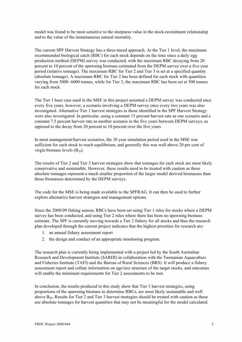
The equation for the catch curve regression for blue mackerel in the west (South Australia; pooled across years) is:
6921.91278.1)ln( +−= AN where N is the number of fish and A is the age group (years) (Figure 2.5).
0 1 2 3 4 5 6 7
Age (Years)
Nat
ural
Log
arith
m o
f Fre
quen
cy
01
23
45
67
89
10
Blue mackerel (west)
0 1 2 3 4
Age (Years)
Sele
ctiv
ity
0.0
0.1
0.2
0.3
0.4
0.5
0.6
0.7
0.8
0.9
1.0
1.1
1.2
Blue mackerel (west)
Figure 2.5: Catch curve and selectivity curve for blue mackerel (west). Hoenig’s (1983) equation was used to determine M for blue mackerel (both east and west stocks):
)log(982.044.1 AgeMaximumeM −= where AgeMaximum for blue mackerel is 7 years. The proportion of sexually mature fish-at-age, af , was obtained from Knuckey et al. (2008). Table 2.5 provides the input data for blue mackerel (east) used in the MSE operating model (see Chapter 3) as specified above. The spawning biomass estimate for blue mackerel (east) in 2005 from the DEPM was 23 009 tonnes (Ward and Rogers, 2007). Table 2.6 provides the input data for blue mackerel (west) used in the MSE operating model (see Chapter 3) as specified above. The spawning biomass estimate for blue mackerel (west) in 2005 from the DEPM was 56 288 tonnes (Ward and Rogers, 2007).

Table 2.5: Input data for blue mackerel (east) used in the MSE operating model.
Age Sample
Frequency Catch Curve Frequency
aN ,0 – Data Proportions
aN ,0 – EquilibriumProportions
aM – Natural Mortality
aS Selectivity
aw Weight
af – Proportion of Sexually Mature Fish
0 1057 47572 0.462 0.462 0.62 0.022 96.01 0 1 2045 9648 0.249 0.249 0.62 0.212 209.46 0 2 1817 1957 0.206 0.134 0.62 1.000 336.32 1 3 613 397 0.069 0.072 0.62 1.000 426.72 1
4+ 125 100 0.014 0.084 0.62 1.000 545.23 1
Table 2.6: Input data for blue mackerel (west) used in the MSE operating model.
Age Sample
Frequency Catch Curve Frequency
aN ,0 – Data Proportions
aN ,0 – EquilibriumProportions
aM – Natural Mortality
aS Selectivity
aw Weight
af – Proportion of Sexually Mature Fish
0 140 16189 0.462 0.462 0.62 0.008 80.85 0 1 635 5241 0.249 0.249 0.62 0.121 184.31 0 2 691 1697 0.111 0.134 0.62 1.000 338.43 1 3 566 549 0.091 0.072 0.62 1.000 477.26 1
4+ 547 261 0.088 0.084 0.62 1.000 583.22 1
FRD
C Project 2008/064
14

FRDC Project 2008/064 15
2.1.3. Jack mackerel Data for jack mackerel (Trachurus declivis) were derived from Browne (2005). Data for the 2003/04 fishing season were used to derive the age structure of the stock, however, the length-weight relationship used was that determined by Williams et al. (1987) for the 1986/87 season. This was then used to obtain an estimate of the average weight-at-age. Length measurements were obtained for 5461 jack mackerel during the 2003/04 fishing season, and these were weighted to the total catch in each shot where samples were taken. The length-weight relationship used for jack mackerel was from Williams et al. (1987):
)(log097.3021.2)(log 1010 FLW +−= where W is body weight (g) and FL is fork length (mm). There was no zero age group in the age-length key, so a regression on the weights for the other ages was used to estimate this value. The weights estimated by the regression were used for all age groups (Figure 2.6). The regression equation is:
753.30576.51 += AW
Age (Years)
Wei
ght (
gram
s)
010
020
030
040
050
060
0
0 1 2 3 4 5 6 7 8 9 10
Jack mackerel
Figure 2.6: Age-weight relationship for jack mackerel. The equation for the catch curve regression for jack mackerel is:
966.155141.0)ln( +−= AN where N is the number of fish and A is the age group (years) (Figure 2.7).

FRDC Project 2008/064 16
Age (Years)
Nat
ural
Log
arith
m o
f Fre
quen
cy
02
46
810
1214
1618
0 2 4 6 8 10 12 14 16 18
Jack mackerel
0 2 4 6 8 10
Age (Years)
Sele
ctiv
ity
0.0
0.1
0.2
0.3
0.4
0.5
0.6
0.7
0.8
0.9
1.0
1.1
1.2
Jack mackerel
Figure 2.7: Catch curve and selectivity curve for jack mackerel. Hoenig’s (1983) equation was used to determine natural mortality ( M ) for jack mackerel:
)log(982.044.1 AgeMaximumeM −= where AgeMaximum for jack mackerel is 17 years. The proportion of sexually mature fish-at-age, af , was obtained from Knuckey et al. (2008). Table 2.7 provides the input data for jack mackerel used in the MSE operating model (see Chapter 3) as specified above. There was no spawning biomass estimate for jack mackerel as there has been no DEPM estimate for this species.
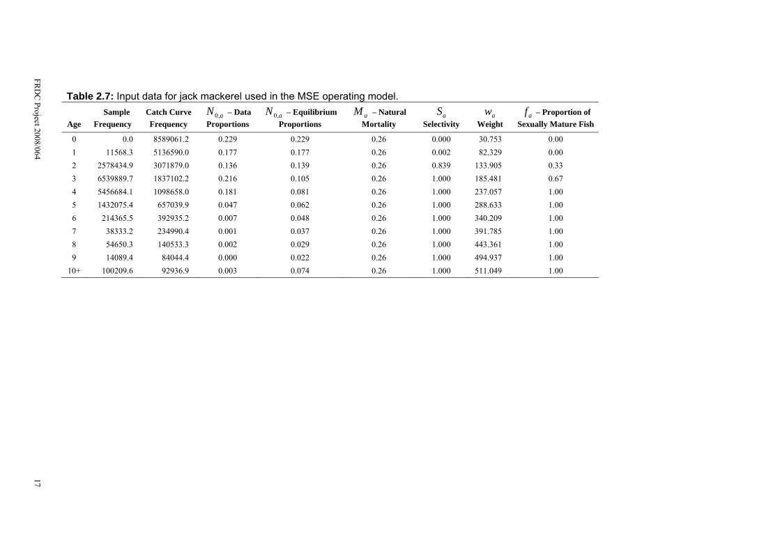
Table 2.7: Input data for jack mackerel used in the MSE operating model.
Age Sample
Frequency Catch Curve Frequency
aN ,0 – DataProportions
aN ,0 – EquilibriumProportions
aM – Natural Mortality
aS Selectivity
aw Weight
af – Proportion of Sexually Mature Fish
0 0.0 8589061.2 0.229 0.229 0.26 0.000 30.753 0.00 1 11568.3 5136590.0 0.177 0.177 0.26 0.002 82.329 0.00 2 2578434.9 3071879.0 0.136 0.139 0.26 0.839 133.905 0.33 3 6539889.7 1837102.2 0.216 0.105 0.26 1.000 185.481 0.67 4 5456684.1 1098658.0 0.181 0.081 0.26 1.000 237.057 1.00 5 1432075.4 657039.9 0.047 0.062 0.26 1.000 288.633 1.00 6 214365.5 392935.2 0.007 0.048 0.26 1.000 340.209 1.00 7 38333.2 234990.4 0.001 0.037 0.26 1.000 391.785 1.00 8 54650.3 140533.3 0.002 0.029 0.26 1.000 443.361 1.00 9 14089.4 84044.4 0.000 0.022 0.26 1.000 494.937 1.00
10+ 100209.6 92936.9 0.003 0.074 0.26 1.000 511.049 1.00
FRD
C Project 2008/064
17

FRDC Project 2008/064 18
2.1.4. Australian sardine (east) Data (unpublished) for Australian sardine off the coast of New South Wales (NSW) were provided by the NSWDPI. Length frequencies from the NSW monitoring program were provided, together with an age composition for landings. Otoliths collected from these samples have not been aged. The age composition and von Bertalanffy growth parameters provided were determined by the NSWDPI from otolith weights, using a regression derived by Rogers and Ward (2007) for South Australian (SA) sardines (John Stewart, pers. comm.). The length frequency data were used to determine average weight for each age group. A total of 5146 fish were measured over four fishing seasons (Table 2.8). Data from all seasons were pooled to obtain the frequencies in each age group.
Table 2.8: Number of Australian sardine (east) sampled in each fishing season (2004/05 to 2007/08).
Season Number 2004/05 249 2005/06 592 2006/07 3096 2007/08 1209
Total 5146
The length-weight relationship used was obtained from FishBase:
1.3009.0 FLW = where W is body weight (g) and FL is fork length (mm). The von Bertalanffy growth parameters used to determine ages from lengths were provided by the NSWDPI (John Stewart, pers. comm.) (Table 2.9).
Table 2.9: Von Bertalanffy growth parameters for Australian sardine. Parameter Value
∞L 236.1 mm FL
K 0.37 yr-1
0t -0.28 years
The equation for the catch curve regression for Australian sardine (east) pooled across years is:
116.9135.1)ln( +−= AN where N is the number of fish and A is the age group (years) (Figure 2.8).

FRDC Project 2008/064 19
0 1 2 3 4 5
Age (Years)
Nat
ural
Log
arith
m o
f Fre
quen
cy
01
23
45
67
89
10
Australian sardine (east)
0 1 2 3 4 5
Age (Years)
Sele
ctiv
ity
0.0
0.1
0.2
0.3
0.4
0.5
0.6
0.7
0.8
0.9
1.0
1.1
1.2
Australian sardine (east)
Figure 2.8: Catch curve and selectivity curve for Australian sardine (east). Hoenig’s (1983) equation was used to determine natural mortality ( M ) for Australian sardine:
)log(982.044.1 AgeMaximumeM −= where AgeMaximum for Australian sardine is 7 years. The proportion of sexually mature fish-at-age, af , was obtained from Knuckey et al. (2008). Table 2.10 provides the input data for Australian sardine (east) used in the MSE operating model (see Chapter 3) as specified above. The spawning biomass estimate for Australian sardine (east) in 2005 from the DEPM was 28 809 tonnes (Ward and Rogers, 2007).

Table 2.10: Input data for Australian sardine (east) used in the MSE operating model.
Age Sample
Frequency Catch Curve Frequency
aN ,0 – DataProportions
aN ,0 – EquilibriumProportions
aM – Natural Mortality
aS Selectivity
aw Weight
af – Proportion of Sexually Mature Fish
0 31 9100 0.462 0.462 0.62 0.003 5.67 0.0 1 354 2925 0.249 0.249 0.62 0.121 17.16 0.5 2 666 940 0.155 0.134 0.62 1.000 40.78 1.0 3 405 302 0.094 0.072 0.62 1.000 64.22 1.0 4 152 97 0.035 0.039 0.62 1.000 88.20 1.0
5+ 21 44 0.005 0.045 0.62 1.000 119.32 1.0
FRD
C Project 2008/064
20

FRDC Project 2008/064 21
2.1.5. Australian sardine (west) – Test case Data (unpublished) for Australian sardine collected from SA were used as a test case for the MSE operating model to evaluate its effectiveness and robustness. The SA test case has a more comprehensive time series of information, particularly with respect to DEPM-based biomass estimates; unlike the stocks in the SPF. Historical data for the SA Pilchard Fishery were provided by SARDI (Tim Ward pers. comm.). Data for spawning biomass estimates have been collected since 1998 (Table 2.11).
Table 2.11: Spawning biomass estimates and catches for Australian sardine (west) in SA test case, 1998 to 2007.
Year Biomass Lower 95% Upper 95% Catch (t)
1998 169635.169 68284.514 133106.227 7312 1999 22910.909 9278.892 17678.718 4080 2000 112357.931 38740.871 66039.025 3290 2001 74207.460 25486.846 38928.995 7507 2002 180787.251 75243.901 152885.747 14450 2003 169958.574 55015.554 132302.242 26137 2004 169207.898 64237.941 109730.197 36631 2005 152066.931 51169.641 96936.791 42475 2006 202635.000 82223.619 157376.971 28626 2007 262990.069 96863.960 160845.377 30355
Average weights-at-age were also provided by SARDI (Table 2.12). Year zero fish were separated into classes of 0.1 years. These were averaged to produce a single weight for age zero fish.
Table 2.12: Weight-at-age data for Australian Sardine (west), provided by SARDI. Age (years) Length (mm) Weight (g) 0.1 33.3 2.8 0.2 42.1 3.4 0.3 50.4 4.1 0.4 58.2 4.8 0.5 65.6 5.6 0.6 72.6 6.5 0.7 79.3 7.5 0.8 85.5 8.6 0.9 91.5 9.7 1 97.1 11.0 2 138.8 26.2 3 162.7 43.5 4 176.3 58.9 5 184.1 69.5 6 188.6 76.3 7 191.1 80.5

FRDC Project 2008/064 22
The equation for the catch curve regression for Australian sardine (west) is: 326.124539.1)ln( +−= AN
where N is the number of fish and A is the age group (years) (Figure 2.9).
0 1 2 3 4 5 6
Age (Years)
Nat
ural
Log
arith
m o
f Fre
quen
cy
02
46
810
1214
Australian sardine (west)
0 1 2 3 4 5
Age (Years)
Sele
ctiv
ity
0.0
0.1
0.2
0.3
0.4
0.5
0.6
0.7
0.8
0.9
1.0
1.1
1.2
Australian sardine (west)
Figure 2.9: Catch curve and selectivity curve for Australian sardine (west) in SA test case. Hoenig’s (1983) equation was used to determine natural mortality ( M ) for Australian sardine (west):
)log(982.044.1 AgeMaximumeM −= where AgeMaximum for Australian sardine is 7 years. SARDI (unpublished) provided an estimate for the age-at-sexual maturity, where 50 percent are mature at age two. Table 2.13 provides the input data for Australian sardine (west) used in the MSE operating model (see Chapter 3) as specified above. There are no zero-age fish in the age frequency because there are few fish of this age class sampled in the fishing area. The weight estimates were obtained from fishery-independent surveys.

Table 2.13: Input data for Australian sardine (west) in SA test case used in the MSE operating model.
Age Sample
Frequency Catch Curve Frequency
aN ,0 – DataProportions
aN ,0 – EquilibriumProportions
aM – Natural Mortality
aS Selectivity
aw Weight
af – Proportion of Sexually Mature Fish
0 0 225483 0.462 0.462 0.62 0.000 5.91 0.0 1 228 52686 0.249 0.249 0.62 0.004 11.00 0.0 2 877 12310 0.134 0.134 0.62 0.071 26.16 0.5 3 1673 2876 0.083 0.072 0.62 1.000 43.50 1.0 4 1191 672 0.059 0.039 0.62 1.000 58.90 1.0
5+ 276 203 0.014 0.045 0.62 1.000 75.42 1.0
FRD
C Project 2008/064
23

FRDC Project 2008/064 24
3. Management Strategy Evaluation (MSE)
3.1. Introduction The three assessment tiers in the SPF Harvest Strategy (see Appendix C) require different levels of data and assessment:
• a Tier 3 assessment relies on catch and effort information, with some knowledge of the biology of the species
• a Tier 2 assessment uses catch and effort information, and knowledge of the biology of the species, combined with age data from an appropriate sampling regime
• a Tier 1 assessment relies on DEPM surveys, as well as catch and effort information, biology, and ageing data.
In 2007, a consultant was hired by AFMA to review the draft SPF Harvest Strategy (Knuckey et al. 2008), which included an MSE based on a simple population model and data taken from relevant literature. They presented results for a number of management scenarios based on the Tier 1 assessment for the harvest strategy. SPFRAG found the results of the modelling exercise extremely valuable and requested the MSE be run for alternative harvest scenarios, including Tier 2 and Tier 3 based scenarios; as well as using actual data collected in the field such as through DEPM surveys and age collections, to condition the operating model used in the MSE. Whilst Knuckey et al. (2008) provided a description of the model used, the computer code used to implement the MSE was not made available to the SPFRAG. One of the objectives of our project was to build on the equations provided in the Knuckey et al. (2008) review to develop an MSE and use it to evaluate a number of management/harvest scenarios, using actual data where available. Where data from the fishery were not available, assumptions were made using data from other sources. Actual biological data included in the MSE were collected for redbait (east and west stocks), blue mackerel (east and west stocks), jack mackerel and Australian sardine (east). These data included estimates of spawning biomass (not available for redbait west or jack mackerel), and length and age of adult fish collected through fishing activities (available for all stocks). A test case was also conducted for Australian sardine (west) off the coast of SA as a more comprehensive time series of age and DEPM survey data for this stock were available. This enabled a potentially more robust test of the MSE than that provided by the data-limited SPF stocks. The new MSE has been developed using the R statistical package (version 2.8.0, www.r-project.org; see Appendix D for model code). Changes have been made to the operating model equations used in Knuckey et al. (2008) including adding the Beverton-Holt stock-recruitment relationship to investigate the sensitivity of the MSE to stock-recruitment assumptions. Testing of the harvest strategy under Tier 2 and Tier 3 conditions was not investigated in Knuckey et al. (2008) but has been done in our project with the new MSE. The new MSE framework aims to provide a starting point for the exploration of different harvest strategies, as well as highlighting where additional data and research could give the most benefit in our understanding of the dynamics of the SPF and approaches needed to manage the fishery. The MSE has been conditioned for the four target species of the SPF; redbait, blue mackerel, jack mackerel and Australian sardine. For the first three species, management has been implemented by dividing them into eastern (labelled A) and western (labelled B) stocks. For the eastern stock of redbait, both stocks of blue mackerel and Australian sardine, the MSE was conditioned on actual data from the fishery (see Chapter 2). For each of the six stocks plus the test case of Australian sardine (west), a range of scenarios were considered which enabled the harvest strategies at each

FRDC Project 2008/064 25
assessment tier level to be investigated, as well as sensitivities of the operating model to key parameters.
3.2. Model description An MSE is a decision-support tool that uses a set of rules and pre-specified data to provide recommendations for management actions, where the performance of the rules is evaluated by simulation (Butterworth and Punt, 1999). It allows users of the tool to investigate the trade-offs among different management objectives for a fishery, and for management decisions to be able to take these trade-offs into account. Conceptually, an MSE includes three main components: (a) the operating model that describes ‘reality’; (b) the management strategies that are to be evaluated; and (c) the performance measures that will be used to evaluate the performance of each management strategy in relation to the objectives (Dichmont et al. 2008). The MSE framework allows for data specific to the fishery and the stock to be included in the operating model, though the framework also allows for uncertainty in these data and model parameter assumptions through investigation of a wide range of plausible scenarios. Agreed management strategies should be robust to these uncertainties, as well as achieving the desired management objectives. The SPF MSE applies a simple age-structured production operating model. The MSE operating model sets up a hypothetical population with the characteristics of the SPF target species by using actual fishery data where available. Management strategies (e.g. TACs), as determined by the harvest strategy, are then enforced on the population during a projected period (e.g. 30 years). The effect of the management decisions on this population is viewed as a reflection of the possible effect on the species in reality. Uncertainty is included in the model through stochastic processes, as well as through an investigation of a range of values for key input parameters (e.g. steepness, natural mortality, etc.). Stochastic components are included in the stock-recruitment relationship, the simulation of the spawning biomass estimate from the DEPM survey and in the determination of the realised catch in each year. Running the MSE in a Monte Carlo fashion, i.e. repeating a model run with the same initial conditions many times over (e.g. 1000 repetitions), allows random variation to be taken into account and the possible risks associated with this variation to be considered.
3.2.1. Population dynamics The operating model population dynamics equations were taken from Haltuch et al. (2008):
⎪⎪⎪
⎩
⎪⎪⎪
⎨
⎧
=−+
−
<≤−
=
=
−−−
−−
−−
−−
−−
−−
−−
+
+−−−
−−−
maeFSeNeN
eFSeNeN
maeFSeNeN
aR
N
aaa
aaa
aaa
Mya
May
May
Mya
May
May
Mya
May
May
y
ay
if ,)(
)(
1 if ,)(
0 if ,
5.05.0,
5.0,
5.01
5.01,
5.01,
5.01
5.01,
5.01,
1
,1111
111
(3.1) where ayN , is the number of fish of age a at the start of year y , aM is the instantaneous rate of
natural mortality at age a , yR is the number of recruits at the start of year y (given by the stock-
recruitment relationship), aS is the fishing selectivity-at-age a , yF is the fully selected

FRDC Project 2008/064 26
exploitation rate in year y and m is the largest age considered. It is assumed that catches are taken as a pulse mid-year (as in Knuckey et al. 2008). Growth, or progression to the next age group, is an instantaneous event that occurs at the beginning of each year. The equilibrium (i.e. time invariant) age-structure when no fishing is occurring can be calculated by the following:
⎪⎪⎪
⎩
⎪⎪⎪
⎨
⎧
=−
<≤
=
=
−
−
−
−−
−
−
mae
eN
maeN
aR
N
a
a
a
M
M
aeq
Maeqaeq
if,)1(
1 if,
0 if,
1
1
1,
1,
0
, (3.2)
where 0R is the average number of recruits in the absence of fishing.
Natural mortality rates at age and selectivities at age have been provided for each stock in Chapter 2. Selectivities at age are assumed to be unchanging with time and natural mortality is assumed to be the same for all ages of a particular stock. Uncertainty around natural mortality has been investigated in simulations, but uncertainty in selectivities has not been explored in this analysis.
0R has been calculated based on the assumed value for *R , the maximum number of recruits, as shown in equation 3.4.
3.2.2. Stock-recruitment The relationship between spawning stock size and the number of recruits is an important assumption of the MSE operating model as it underlies the productivity of the simulated population. This relationship can make a considerable difference to the simulation results, particularly when management scenarios drive the population to low levels of spawners. There are several mathematical models that have been developed to describe the relationship between spawning stock and recruitment including those of Ricker (1954), Beverton and Holt (1957), Deriso (1980), and most recently, the Hockey-stick models (Barrowman and Myers, 2000). Knuckey et al. (2008) used a Hockey-stick model to describe the stock-recruitment dynamics of SPF species. The Hockey-stick model can be described as a two piece function where the relationship for lower numbers of spawners is linear with a positive slope, and the relationship for higher number of spawners is constant at the value of the maximum number of recruits. Where the two functions intersect is called the ‘kink’. Knuckey et al. (2008) assumed the kink to occur at 20 percent of virgin spawning biomass as a base for all SPF species (see Figure 3.1). The Beverton-Holt model uses a smooth curve that approaches the upper bound of number of recruits to describe the relationship between spawners and recruitment. Without investigation into spawner-recruit data from the SPF target species it is difficult to decide on the stock-recruitment relationship that is best suited to modelling these species. It is likely, though, that different SPF species have different stock-recruitment relationships assumed as they may respond differently to having a small number of spawners in the population. The advantage of using the Beverton-Holt stock-recruitment model is that studies have been made of various species’ data to better understand the stock-recruitment relationship at low levels of spawners. In the Beverton-Holt relationship the key parameter for this part of the relationship is commonly referred to as the ‘steepness’. The MSE code allows for the choice between the Hockey-stick and Beverton-Holt stock-recruitment models, however, only the

FRDC Project 2008/064 27
results using the latter model have been presented here with use of the results from Myers et al. (1999) in determining appropriate steepness values for each of the SPF species. The Beverton-Holt relationship used in the formulation is as in Haltuch et al. (2008):
),0(~ ,)15()1(
4 22/01
2
Ryr
spy
sp
spy
y NreBhKh
BhRR Ry σσ−
+ −+−= , (3.3)
where sp
yB is the spawning biomass at the start of year y , h is the steepness of the stock-
recruitment relationship, spK is the virgin spawning biomass and yr is a random number drawn
from a normal distribution with mean zero, variance 2Rσ and serial correlation Rρ .
0R can be defined in terms of *R , where *R is the maximum number of recruits, by the following:
hhRR
4)15(*
0−
= . (3.4)
So, substituting (3.4) into (3.3) gives the following:
),0(~ ,)15()1(
)15( 22/*
1
2
Ryr
spy
sp
spy
y NreBhKh
BRhR Ry σσ−
+ −+−
−= . (3.5)
The term 2/2Ryre σ− is used, as recommended in Hilborn et al. (1992), to capture the random
variation around the stock-recruitment curve which generally has a lognormal distribution when following both theoretical assumptions and observational evidence (see Hilborn et al. 1992 for details). The 2/
2
Rσ− component is a bias-correction term that adjusts the result so that the expected recruitment is equal to the mean recruitment as given by the stock-recruitment relationship without error. This recruitment variation term has the feature of occasionally showing very large recruitment and allowing the amount of variation to be proportional to the average recruitment, so we expect to see lower variability at small recruitments and higher variability at large recruitments. The recruitment variation parameter (along with the other stock-recruitment relationship parameters) can be better estimated through investigation of numbers of spawners to recruits for particular SPF species. In the absence of these actual data we have used the arbitrary values given by Knuckey et al. (2008). As the base case, Knuckey et al. (2008) defined yr as a random number
drawn from a normal distribution with mean 0, standard deviation 6.0=Rσ and no serial correlation. Sensitivity runs were made using a standard deviation of 0.3, and runs assuming a serial correlation of 0.5 were also made in sensitivity analyses. The Beverton-Holt steepness parameter h is defined as the proportion of recruitment relative to the virgin state, when the spawner biomass is reduced to 20 percent of virgin level. Figure 3.1 shows a Beverton-Holt relationship with varying values of h compared to the Hockey-stick relationship with the same value of *R for both stock-recruitment relationships. Knuckey et al. (2008) set *R to an arbitrary value of 800 million recruits for each of the SPF species. Without evidence to suggest otherwise, the same assumption has been made in this work. Myers et al. (1999) carried out an investigation of over 700 spawner-recruitment series to search for constant parameters in the

FRDC Project 2008/064 28
stock-recruitment relationship at the species level or higher. They found that the number of recruits produced per spawner each year at low population levels is relatively constant within species, and that there is relatively little variation between species. Myers et al. (1999) estimated h for a range of species as part of the investigation into spawner-recruitment relationships. Since, most of the SPF species considered in the MSE did not appear in the Myers et al. (1999) study, approximations of h were made by comparing SPF species to those species with similar life history characteristics for which h was estimated.
Figure 3.1: A comparison of the Beverton-Holt stock-recruitment relationship (assuming different steepness values; h) to the Hockey-stick relationship with a kink at 20 percent of virgin spawning biomass. Both stock-recruitment relationships have the same maximum number of recruits and have been plotted assuming no random variation. Knuckey et al. (2008) used a metric developed by Koopman et al. (2000) to compare the life history similarity of SPF species to a range of other species. The metric is based on characteristics of the species such as maximum age, habitat and diet, with small similarity values suggesting the species are somewhat similar and large values suggesting they are not (for details see Koopman et al. 2000). Knuckey et al. (2008) looked at all species which scored less than two when compared to SPF species. Table 3.1 shows the three matched species in terms of lowest scores with each of the

FRDC Project 2008/064 29
SPF species that also appeared in Myers et al. (1999). The corresponding steepness ( h ) values for those matched species have then been assigned. In some cases a 20th and 80th percentile value for h was included in Myers et al. (1999), as well as the median. For each species a steepness value was chosen and the sensitivity of this value investigated by running scenarios with values of h ± h2.0 of the chosen value. The values used are shown in Table 3.2.
Table 3.1: For each of the four SPF species, the three most similar species based on their life histories that appear in Myers et al. (1999) are identified. How similar a species is to another has been determined using the metric developed by Koopman et al. (2000). For each match, the similarity value is given, as well as the median steepness value (hmed as used in the Beverton-Holt stock-recruitment relationship) and in some cases a 20th (h20) and 80th (h80) percentile steepness value is also given. A range of similarity values is provided for herring indicating differences between stocks for that species. SPF species Matched species Similarity value h20 hmed h80
Redbait Herring Clupea harengus 0.83-1.77 0.52 0.74 0.88 Emmelichthys nitidus Haddock Melanogrammus aeglefinus 1.73 0.64 0.74 0.82 Saithe Pollachius virens 1.73 0.78 0.81 0.84 Blue mackerel Northern anchovy Engraulis mordax 0.2 0.43 Scomber australasicus Gulf menhaden Brevoortia patronus 0.83 0.57 Sprat Sprattus sprattus 0.83 0.48 0.65 0.79 Chub mackerel Scomber japonicus 0.38 Atlantic mackerel Scomber scombrus 0.62 0.81 0.92 Sardine Sardinops sagax 1.11 0.34 0.59 0.81 Jack mackerel Herring Clupea harengus 0.5-1.87 0.52 0.74 0.88 Trachurus declivis Spanish sardine Sardina pilchardus 0.53 0.34 T. murphyi Horse mackerel Trachurus trachurus 0.75 Pacific sardine Sardinops sagax 1.36 0.34 0.59 0.81 Australian sardine Northern anchovy Engraulis mordax 0.2 0.43 Sardinops sagax Gulf menhaden Brevoortia patronus 0.83 0.57 Sprat Sprattus sprattus 0.83 0.48 0.65 0.79 Pacific sardine Sardinops sagax 1.11 0.34 0.59 0.81
Discussions with SPFRAG suggested that the SPF target species would fall into two groups with similarities between redbait and jack mackerel, and blue mackerel and Australian sardine. Steepness values were chosen from species studied by Myers et al. (1999) using two methods. Either species of the same family were chosen, or they were based on the similarity index developed by Koopman et al. (2000). The steepness value used for Australian sardine was that determined by Myers et al. (1999) for Pacific sardine, as these are the same species. For blue mackerel, the mean of chub mackerel and Atlantic mackerel (which are from the same family) is 0.60, and is close to the 0.59 of sardine, which was the value used. Blue mackerel and sardine have a good similarity rating using the Koopman et al. (2000) index. The steepness value determined for horse mackerel by Myers et al. (1999) was chosen for use with jack mackerel as these two species are from the same family. The steepness value used for redbait was that determined by Myers et al. (1999) for herring as these had a good similarity rating using the Koopman et al. (2000) index. Table 3.2 gives a summary of the steepness values chosen for each species and shows that, as the SPFRAG suggested, redbait and jack mackerel are similar to each other, as are blue mackerel and Australian sardine.

FRDC Project 2008/064 30
Table 3.2: The steepness values used for each of the SPF species in the MSE operating model. For most runs the steepness value hbase is used where hbase corresponds to the median steepness value of the matched species chosen in Table 3.1 to be representative of the SPF species. The steepness values hsensitivity are ±20 percent of the hbase value and are used in testing the sensitivity of the model to the choice of h. hbase hsensitivity
Redbait 0.74 0.89, 0.59 Blue mackerel 0.59 0.71, 0.47 Jack mackerel 0.75 0.90, 0.60 Australian sardine 0.59 0.71, 0.47
3.2.3. Spawning biomass The ‘true’ spawning biomass at the start of year y , or the spawning biomass of the modelled population at the beginning of a simulated year, is given by:
aa
m
aay
spy fwNB ∑=
=1, , (3.6)
where aw is the weight of a fish of age a at the start of the year and af is the proportion of fish at sexual maturity at age a . Both of these parameter values have been determined by the data as described in Chapter 2. In testing harvest strategies at the Tier 1 level, the operating model simulates estimating spawning biomass through conducting DEPM surveys. This is done by multiplying the true spawning biomass by an error term with a lognormal distribution,
ωeBB spy
survy = , (3.7)
where ω is a random number drawn from a normal distribution with mean zero and standard deviation 3.0=survσ . The virgin spawning biomass (Ksp) is the spawning biomass under unexploited equilibrium conditions as described by equation 3.2. It is calculated by:
∑=
=m
aaaaeq
sp fwNK1
, . (3.8)
3.2.4. Catches For each simulated year, a TAC is set. The TAC is dependent on the harvest strategy being tested in the MSE. The details of how the SPF Harvest Strategy is implemented in the model are in the next section (3.3). Only one of two alternatives can occur — either the TAC is independent of spawning biomass, i.e. no DEPM surveys have been conducted so the TAC is set under Tier 2 or Tier 3 of the harvest strategy, or a proportion of the estimated spawning biomass is set as the TAC, i.e. a Tier 1 implementation of the harvest strategy. If the latter, then
survyy pBTAC = , (3.9)

FRDC Project 2008/064 31
where survyB is the spawning biomass estimate from the most recent simulated DEPM survey and
p is the proportion of the estimated spawning biomass which may be taken as catch as stipulated by the harvest strategy, and is dependent on the age of the survey (see Appendix C). The catches are assumed to be taken as a pulse mid-year, with catches constrained to no more than 95 percent of the exploitable biomass. The mid-year exploitable biomass, where aS is the fishing selectivity-at-age a and m is the oldest age considered as defined for equation 3.1, is calculated by:
mmM
myaaMm
aay
exy SweNSweNB ma 5.0
,5.05.01
1,
−+
−−
=+∑= (3.10)
where 15.0 ++ = aaa www .
The realised catch is then the TAC multiplied by any implementation error. Implementation error was not taken into account in the MSE developed by Knuckey et al. (2008). This error allows for the inclusion of uncertainty in the relationship between the TAC recommended by management and the actual catch in the model. In order to get a better idea of how this error should be characterised, analysis of SPF catch and TAC data is recommended. In this model, a Beta distribution was used to randomly generate implementation error. The Beta distribution is a family of probability distributions defined on the interval [0, 1] and parameterised by two positive shape parameters denoted by α and β . Figure 3.2 shows the probability density function for several Beta distributions with different values of α and β. If implementation error is included in the model then the realised catch in year y is calculated by:
),( βαBetaTACC yy = , (3.11)
where ),( βαBeta is a random number drawn from a Beta distribution with shape parameters α and β . In the operating model, parameter values of 10=α and 1=β were assumed, giving an expected value of 0.91 (i.e. on average, 91 percent of the TAC is realised). These values may be revised once the recommended work has been conducted. Scenarios where there is no implementation error have also been investigated for each of the different strategies. In these cases the realised catch is assumed to be equal to the TAC. The fully selected exploitation rate per year, yF , is then calculated by:
⎪⎩
⎪⎨
⎧≤
=
otherwise. ,95.0
0.95 if , exy
yexy
y
y BC
BC
F (3.12)

FRDC Project 2008/064 32
Figure 3.2: The probability density function for the Beta distribution using different values for the shape parameters α and β. The dashed curves have a constant value for β and look at the effect of changing α. The bold curves keep α constant and change β. The distributions with high density at values close to 1 represent those where there is little implementation error, i.e. the realised catch is approximately equal to the TAC.
3.3. Implementation of the harvest strategy in the model Some assumptions were needed to be made when implementing the SPF Harvest Strategy (see Appendix C) in the MSE. For Tier 1 MSEs, it was assumed that there is a year’s lag between a DEPM survey being conducted and its use in setting a TAC. It is also assumed that, in the first year of simulation, a survey has become available (i.e. a survey was conducted the year before) and no surveys have been conducted prior to this one. For all tiers, the TAC is set at the start of each simulated year. For Tier 1 MSEs of species where DEPM survey estimates of spawning biomass were available, there was a request by SPFRAG for these estimates to be used in the MSE. The operating model

FRDC Project 2008/064 33
for this MSE, though being further developed from the model used in Knuckey et al. (2008), has not been implemented to allow fitting to available catch and DEPM survey data. For this to happen, a longer time series of survey data would be needed, as well as a more complex statistical based operating model framework. Using a statistical operating model would enable the plausibility of assumed model parameters to be assessed in relation to data obtained from the fishery to give an indication of which parameterisations would be most likely. With only at most two DEPM surveys having been conducted for any of the SPF stocks, a more complex model is not defensible at this stage. In order to use the DEPM estimate in the MSE in some way, a scenario was run for species where DEPM estimates were available using the most recent DEPM estimate as the starting spawning biomass to the simulation. As the error associated with the DEPM estimates is unknown, using the actual estimate as the starting spawning biomass in simulations can highlight where assumptions of data and model parameters may be unrealistic. As detailed above in the model equations, an estimate of the virgin spawning biomass can be calculated given weight-at-age, fecundity-at-age, mortality-at-age, steepness in the Beverton-Holt stock-recruitment relationship and an estimate of the expected number of recruits. If there is error in any or all of these values, as there is likely to be, then the actual DEPM spawning biomass estimate may not make sense when compared to the calculated virgin spawning biomass (i.e. it may be many times larger or considerably smaller than is believed to be the case). Also, the error in the DEPM estimate itself is confounded in all this. Generally, these types of simple MSEs concentrate on the relative effectiveness (or trend) of the management strategies being investigated rather than using the MSE to give an absolute estimate of the current spawning biomass as is done in traditional stock assessments. Tier 1 as implemented in the MSEs (and harvest strategy), set the TACs relative to spawning biomass estimates, i.e. it takes a pre-defined percentage of the spawning biomass estimate from the DEPM survey. So, investigating different starting points of current spawning biomass in terms of percentage of virgin spawning biomass, along with incorporating scenarios that account for the uncertainty in key model parameters, is generally sufficient in being able to measure the relative effect (or trend) of a Tier 1 MSE on the population of interest without needing to know the actual spawning biomass. When testing a Tier 2 implementation of the SPF Harvest Strategy, the TACs are set to the RBC for the particular species within a particular management zone and for a Tier 3 implementation, the TAC is set to 500 t (at a maximum) for each species within each management zone. Using actual values in setting TACs in the model, rather than proportions as in Tier 1 simulations, can again highlight problems in either the initial model set-up in terms of biological information about the species (e.g. natural mortality rates, stock-recruitment relationship, etc.), as well as in the choices of RBCs. Unlike the MSE for a Tier 1 strategy, the results of the MSE for Tiers 2 and 3 may not be useful if the parameter values assumed are not accurate.
3.4. Performance statistics Performance statistics are used to compare model runs under different parameter assumptions and harvest strategies. The performance statistics should be indicative of what the management strategies are intending to achieve. The performance statistics used in the MSE are:
1. the spawning biomass at the last year of simulation as a percentage of the virgin spawning biomass
2. the median catch over all years of simulation 3. the catch coefficient of variation (CV), i.e. the ratio of the standard deviation of catch to
mean catch over all years of simulation 4. the percentage risk for B20 (20 percent of virgin spawning biomass) where percentage risk
FRDC Project 2008/064 34
is defined as the percentage of years over all repetitions of a scenario where the spawning biomass fell below B20 (see Figure 3.3)
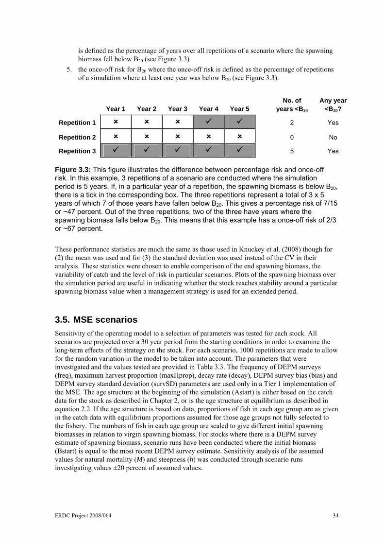
5. the once-off risk for B20 where the once-off risk is defined as the percentage of repetitions of a simulation where at least one year was below B20 (see Figure 3.3).
Year 1 Year 2 Year 3 Year 4 Year 5 No. of
years <B20 Any year
<B20?
Repetition 1 2 Yes
Repetition 2 0 No
Repetition 3 5 Yes
Figure 3.3: This figure illustrates the difference between percentage risk and once-off risk. In this example, 3 repetitions of a scenario are conducted where the simulation period is 5 years. If, in a particular year of a repetition, the spawning biomass is below B20, there is a tick in the corresponding box. The three repetitions represent a total of 3 x 5 years of which 7 of those years have fallen below B20. This gives a percentage risk of 7/15 or ~47 percent. Out of the three repetitions, two of the three have years where the spawning biomass falls below B20. This means that this example has a once-off risk of 2/3 or ~67 percent.
These performance statistics are much the same as those used in Knuckey et al. (2008) though for (2) the mean was used and for (3) the standard deviation was used instead of the CV in their analysis. These statistics were chosen to enable comparison of the end spawning biomass, the variability of catch and the level of risk in particular scenarios. Plots of the spawning biomass over the simulation period are useful in indicating whether the stock reaches stability around a particular spawning biomass value when a management strategy is used for an extended period.
3.5. MSE scenarios Sensitivity of the operating model to a selection of parameters was tested for each stock. All scenarios are projected over a 30 year period from the starting conditions in order to examine the long-term effects of the strategy on the stock. For each scenario, 1000 repetitions are made to allow for the random variation in the model to be taken into account. The parameters that were investigated and the values tested are provided in Table 3.3. The frequency of DEPM surveys (freq), maximum harvest proportion (maxHprop), decay rate (decay), DEPM survey bias (bias) and DEPM survey standard deviation (survSD) parameters are used only in a Tier 1 implementation of the MSE. The age structure at the beginning of the simulation (Astart) is either based on the catch data for the stock as described in Chapter 2, or is the age structure at equilibrium as described in equation 2.2. If the age structure is based on data, proportions of fish in each age group are as given in the catch data with equilibrium proportions assumed for those age groups not fully selected to the fishery. The numbers of fish in each age group are scaled to give different initial spawning biomasses in relation to virgin spawning biomass. For stocks where there is a DEPM survey estimate of spawning biomass, scenario runs have been conducted where the initial biomass (Bstart) is equal to the most recent DEPM survey estimate. Sensitivity analysis of the assumed values for natural mortality (M) and steepness (h) was conducted through scenario runs investigating values ±20 percent of assumed values.

FRDC Project 2008/064 35
Table 3.3: Parameters investigated in scenarios along with the particular values that were tested. Factor Values Frequency of DEPM surveys (freq) 1/2, 1/5 (i.e. 1 in 2 years or 1 in 5 years) Maximum harvest proportion (maxHprop) 0.2, 0.15, 0.075 (i.e. 20%, 15% or 7.5% of survey estimate) Decay rate of harvest proportion (decay) 0.025, 0 (i.e. decay by 2.5% or no decay) DEPM survey bias (bias) No bias, 50% Natural mortality (M) Base value, Base value ±20% Steepness (h) hbase , hsensitivity (upper and lower values) Implementation error (ierror) Yes, No Starting age structure (Astart) Data, Equilibrium Recruitment variation (SRvari) 0.6, 0.3 Recruitment serial correlation, (SRcorr) 0, 0.5 DEPM survey standard deviation (survSD) 0.3, 0.6 Initial biomass as % of B0 (Bstart) 90%, 100%, 70%, 50%, DEPM (where available)
The Tier 1 scenarios investigated for each stock are in Table 3.4. The Tier 2 and Tier 3 scenarios investigated for each stock are in Table 3.5. A ‘no harvest’ scenario was also investigated for each stock. This scenario has been included in Table 3.4, though it does not fit with any of the tier scenarios as no catch is being taken from the population. This scenario is used to characterise the population dynamics of the species when no fishing is occurring. For each of the tier approaches, a base case (assumed to best represent reality) has been defined for the purpose of comparison. All other scenarios stem from this base case with, in most cases, only one parameter different between the base and alternative scenario cases. The performance statistics relating to all scenario runs for each stock along with plots of spawning biomass over the simulation period for each run can be found in Appendix E.

Table 3.4: The parameter specifications for Tier 1 assessment scenarios that were investigated for each of the six stocks and the test case. The highlighted values indicate the differences to the base case. Runs denoted with a * could only be made for those stocks with DEPM spawning biomass estimates. Scenario 1 is a ‘no harvest’ scenario.
Scenario freq maxHprop decay bias M h ierror Astart SRvari SRcorr survSD Bstart 1 - - - - M hbase - Equilibrium 0.6 0 - 100%
Tier 1 Base 2 1/5 0.20 0.025 0 M hbase Yes Data 0.6 0 0.3 90% 3 1/5 0.20 0.025 0 M hupper Yes Data 0.6 0 0.3 90% 4 1/5 0.20 0.025 0 M hlower Yes Data 0.6 0 0.3 90% 5 1/5 0.20 0.025 0 M hbase Yes Data 0.3 0 0.3 90% 6 1/2 0.20 0.025 0 M hbase Yes Data 0.6 0 0.3 90% 7 1/5 0.20 0.025 0 M hbase Yes Data 0.6 0 0.6 90% 8 1/5 0.20 0.025 0 M hbase Yes Data 0.6 0.5 0.3 90% 9 1/5 0.20 0.025 0 M hbase Yes Data 0.6 0 0.3 100%
10 1/5 0.20 0.025 0 M hbase Yes Data 0.6 0 0.3 70% 11 1/5 0.20 0.025 0 M hbase Yes Data 0.6 0 0.3 50%
*12 1/5 0.20 0.025 0 M hbase Yes Data 0.6 0 0.3 DEPM *13 1/5 0.20 0.025 0 M+20% hbase Yes Data 0.6 0 0.3 DEPM *14 1/5 0.20 0.025 0 M-20% hbase Yes Data 0.6 0 0.3 DEPM 15 1/5 0.20 0.025 0 M hbase No Data 0.6 0 0.3 90% 16 1/5 0.20 0.025 0 M hbase Yes Equilibrium 0.6 0 0.3 90% 17 1/5 0.20 0.025 0 M+20% hbase Yes Data 0.6 0 0.3 90% 18 1/5 0.20 0.025 0 M-20% hbase Yes Data 0.6 0 0.3 90% 19 1/5 0.20 0.025 50% M hbase No Data 0.6 0 0.3 90% 20 1/5 0.15 0 0 M hbase No Data 0.6 0 0.3 90% 21 1/5 0.075 0 0 M hbase No Data 0.6 0 0.3 90%
FRD
C Project 2008/064
36

FRDC Project 2008/064 37
Table 3.5: The parameter specifications for the Tier 2 and Tier 3 assessment scenarios that were tested for each of the six stocks and the test case. The highlighted values indicate the differences to the base case. The maximum TAC is in tonnes with the Tier 2 values being the RBC in the SPF Harvest Strategy (see Appendix C). For those stocks without DEPM spawning biomass estimates, the run denoted with a * was made using a maximum TAC of 7.5 percent of the model calculated virgin spawning biomass and with a starting biomass of 90 percent of virgin spawning biomass. The scenario denoted ** was not done for those stocks without a DEPM spawning biomass estimate.
Scenario Max. TAC M h Ierror Astart SRvari SRcorr Bstart
Tier 2 Base 22 RBC M hbase Yes Data 0.6 0 90% 23 RBC M hupper Yes Data 0.6 0 90% 24 RBC M hlower Yes Data 0.6 0 90%
*25 7.5% of DEPM M hbase Yes Data 0.6 0 DEPM 26 RBC M hbase No Data 0.6 0 90% 27 RBC M+20% hbase Yes Data 0.6 0 90% 28 RBC M-20% hbase Yes Data 0.6 0 90%
Tier 3 Base 29 500 M hbase Yes Data 0.6 0 90% 30 500 M hupper Yes Data 0.6 0 90% 31 500 M hlower Yes Data 0.6 0 90%
**32 500 M hbase Yes Data 0.6 0 DEPM 33 500 M hbase No Data 0.6 0 90% 34 500 M+20% hbase Yes Data 0.6 0 90% 35 500 M-20% hbase Yes Data 0.6 0 90%
3.6. Test case: Australian sardine (west) Using the data as described in Chapter 2 on Australian sardine found off the coast of SA, we investigated the Tier 1 scenarios as described in Table 3.4. As a 95 percent confidence interval was provided for the 2007 DEPM survey estimate, the upper and lower limits of this range were used as starting spawning biomass levels in scenarios, as well as the estimate itself. We also looked at scenarios combining the two sensitivity steepness values with a starting spawning biomass as given by the DEPM survey estimate. Table 3.6 details these four extra scenarios. To further investigate results, we run all the scenarios using actual DEPM estimates (i.e. the extra scenarios in Table 3.6 plus the scenarios in Table 3.4 that used the DEPM estimates) with the biological characteristics, so weight-at-age, fecundity-at-age and selectivity-at-age, of the SPF Australian sardine (east). The performance statistics relating to all scenario runs for the test case along with plots of spawning biomass over the simulation period for each run can be found in Appendix E.
Table 3.6: The parameter specifications for the extra Tier 1 scenarios investigated for Australian sardine (west). The highlighted values indicate the differences to the base case as described in Table 3.4.
Scenario freq bias M h ierror Astart SRvari SRcorr survSD Bstart
1 1/5 No M hbase Yes Data 0.6 0 0.3 DEPM (upper) 2 1/5 No M hbase Yes Data 0.6 0 0.3 DEPM (lower) 3 1/5 No M hupper Yes Data 0.6 0 0.3 DEPM 4 1/5 No M hlower Yes Data 0.6 0 0.3 DEPM

FRDC Project 2008/064 38
3.7. Results For the six SPF stocks, a summary of the key findings from the MSE scenarios follows. For more detailed results of the MSE testing see Appendix E.
3.7.1. Base case scenarios Table 3.7 gives the performance statistics for all base case scenarios. For Tier 1, the base case scenario resulted in median spawning biomasses after the 30 year projection ranging from 40 percent of virgin spawning biomass for redbait (east) to 68 percent of virgin spawning biomass for blue mackerel (west). The percentage risk was under 3 percent and the once-off risk was under 19 percent for all Tier 1 base case scenarios. The catch CVs for all stocks were between 0.51 and 0.60, though median catches ranged from 2770 t for Australian sardine (east) to 36743 t for jack mackerel. For Tier 2, the base case scenario resulted in median spawning biomasses after the 30 year projection ranging from 36 percent of virgin spawning biomass for Australian sardine (east) to 93 percent of virgin spawning biomass for jack mackerel. Only Australian sardine (east) had a non-zero percentage risk of 0.5 percent and a 3.6 percent once-off risk. As the Tier 2 and Tier 3 scenarios give the absolute catch per year, the catch CV and median catch is of less interest for these tiers. For Tier 3, the base case scenario resulted in median spawning biomasses after the 30 year projection ranging from 90 percent of virgin spawning biomass for Australian sardine (east) to 98 percent of virgin spawning biomass for redbait (west). The risk statistics for all Tier 3 base case scenarios were 0. For all Tier base case scenarios, the last 10-15 years generally show the stock reaching a relatively stable spawning biomass (see Appendix E). Importantly, the zero catch scenarios produced results that would be expected. That is, the starting biomass was set at virgin biomass levels and the model reached equilibrium close to virgin levels in the 30 year simulation period for all stocks. This suggests that the model was behaving according to what would be expected.
3.7.2. Sensitivity analysis As is typical for assessments of this type, the parameters that most effect the performance statistics are those concerned with the stock-recruitment relationship (i.e. steepness) and natural mortality (see Appendix E). Lower steepness values tend to equate to a lower resilience to fishing as the stock produces a proportionally lower number of recruits at lower biomass levels than those populations that have a high steepness value (see Figure 3.1). For all species, the initial biomass and age structure had little impact on the median end spawning biomass. This suggests that the simulated 30 year period was long enough for the stock to reach an equilibrium state, independent of the initial spawning biomass. For the Tier 1 scenarios, lower variation around the stock-recruitment relationship (SRvari) had a lower level of risk associated with it than the base case. There is an increase in risk associated with simulated DEPM survey estimates having more error incorporated into values (survSD). Adding a

FRDC Project 2008/064 39
positive bias of 50 percent to simulated DEPM estimates and including no implementation error resulted in an expected lower end spawning biomass and higher catch and risk than the base case.
Table 3.7: Summary of MSE results for the SPF target stocks and Australian sardine (west) test case for the base case scenarios. Stock Tier End spawning biomass
(%B0) Catch (t) Catch
CV % Risk
B20 Once-off risk B20
Lower Median Upper Lower Median Upper Redbait (east)
1 24.85 39.63 59.07 10885.40 23689.10 49512.93 0.60 2.65 18.90
2 69.21 86.54 112.22 3969.06 4663.03 4948.00 0.09 0.00 0.00 3 77.79 96.28 121.46 396.68 466.36 494.69 0.09 0.00 0.00 Redbait (west)
1 29.86 44.49 62.39 14155.66 29018.35 55361.76 0.53 0.67 7.00
2 71.35 89.77 115.73 3978.56 4668.04 4946.97 0.09 0.00 0.00 3 80.48 97.71 121.30 398.26 466.66 494.89 0.09 0.00 0.00 Blue mackerel (east)
1 37.17 64.41 106.55 7998.77 16480.03 31804.12 0.56 0.34 7.00
2 58.78 89.55 135.65 2377.60 2798.91 2967.81 0.09 0.00 0.00 3 61.58 93.38 138.63 398.78 466.48 494.61 0.09 0.00 0.00 Blue mackerel (west)
1 39.46 67.57 112.25 8213.75 17178.27 32922.46 0.54 0.26 5.40
2 54.88 83.20 130.75 5156.27 6062.05 6429.92 0.09 0.00 0.00 3 63.72 92.83 140.45 396.85 466.03 494.74 0.09 0.00 0.00 Jack mackerel
1 31.77 48.39 70.28 17277.16 36743.20 72575.28 0.55 1.06 11.50
2 72.54 92.79 118.08 3986.03 4662.35 4945.90 0.09 0.00 0.00 3 76.17 95.50 124.48 397.42 467.20 495.03 0.09 0.00 0.00 Australian sardine (east)
1 38.05 65.30 102.57 1362.36 2770.22 5167.73 0.52 0.30 4.70
2 35.73 63.89 104.47 2371.36 2797.31 2968.51 0.09 0.48 3.60 3 62.61 89.75 131.11 397.22 466.40 494.68 0.09 0.00 0.00 Australian sardine (west)
1 41.45 67.12 107.56 735.12 1455.04 2703.17 0.51 0.06 1.70
FRDC Project 2008/064 40
3.7.3. Australian sardine (west) – test case For most scenarios the median end spawning biomass of Australian sardine (west) was between 60-70 percent of virgin spawning biomass (see Appendix E). The last 10 years generally show the stock reaching a relatively stable spawning biomass, with an obvious cyclical pattern if the frequency of DEPM surveys is one in five years. The parameters that make the most difference in performance statistics are steepness and natural mortality. A high steepness generally results in a higher end spawning biomass when compared to the base case and a lower steepness generally results in a lower end spawning biomass than the base case. For the upper sensitivity value of h=0.71, the median end spawning biomass was 70 percent of virgin with a percentage risk of 0.06 percent and once-off risk of 1.60 percent. For the lower sensitivity value of h=0.47, the median end spawning biomass was 63 percent of virgin with a percentage risk of 0.22 percent and once-off risk of 3.70 percent. The assumption for natural mortality had a similar effect with the high mortality assumption of M=0.74 resulting in a median end spawning biomass of 70 percent of virgin spawning biomass and the low mortality assumption of M=0.50 resulting in a median end spawning biomass of 64 percent of virgin spawning biomass. A lower amount of variation around the stock-recruitment relationship (SRvari) had a lower level of risk associated with it than the base case, which is expected, as is the increase in risk associated with simulated DEPM survey estimates having more error incorporated into values (survSD). Adding a positive bias of 50 percent to simulated DEPM estimates and including no implementation error resulted in an expected lower end spawning biomass and higher catch and risk than the base case. The starting biomass levels and age structure had little impact on the end spawning biomass or risk statistics. The actual DEPM survey spawning biomass estimate and upper and lower 95 percent confidence bounds are all much larger than the virgin spawning biomass calculated by the model. This is obvious in the spawning biomass plots in Appendix E, as well as in the high upper 10th percentile of catches over the simulation period. The virgin spawning biomass is calculated using equation 3.8 and is dependent on the maximum number of recruits and steepness as assumed in the stock-recruitment relationship, natural mortality-at-age, weight-at-age, and proportion of sexually mature fish-at-age. As the DEPM estimate of spawning biomass did not seem consistent with the other data, we investigated what assumption of natural mortality would make more sense if the DEPM estimate was reasonably accurate and corresponded to the virgin spawning biomass for this stock. We estimated virgin spawning biomass for different assumed values of natural mortality and compared these values with the DEPM estimate, as well as the upper and lower bounds of the 95 percent confidence interval associated with this estimate (see Figure 3.4). This process gave an estimate of natural mortality between 0.1 and 0.25 which is much lower than the 0.62 assumed in the MSE. The same process was repeated for the sensitivity steepness values of h=0.47 and h=0.59 (see Figure 3.4) as a preliminary investigation of the interaction of steepness with natural mortality in the calculation of virgin spawning biomass. The range of estimates of natural mortality for all steepness values were consistently much lower than 0.62. It should be noted that this method of estimating natural mortality assumes that the 95 percent confidence interval for the DEPM estimate is accurate, as well as assuming no error in the other values on which the virgin spawning biomass is dependent. In order to investigate the inconsistency between the model calculated virgin spawning biomass and the DEPM estimates, a comprehensive study of the potential error in the DEPM survey estimates, as well as in model parameters is recommended as future work (see Chapter 7). In particular, the value assumed for the maximum number of recruits needs to be justified with reference to species and fishery-specific data as this was arbitrarily set to 800 million recruits for all species as was done by Knuckey et al. (2008).

FRDC Project 2008/064 41
Figure 3.4: An investigation into the values of natural mortality, for each of the three assumed steepness values, that would be consistent with the spawning biomass estimate from the 2007 actual DEPM survey for Australian sardine (west) test case. This assumes no error in the other data used to calculate spawning biomass, as well as assuming accuracy in the 95 percent confidence interval for the DEPM estimate. There is also the assumption that the stock is currently at virgin levels. Virgin spawning biomass values are calculated for different assumed values of natural mortality and compared with the DEPM estimate (bold horizontal line) as well as the upper and lower bounds of the 95 percent confidence interval (dashed horizontal lines) associated with this estimate.
3.8. Discussion The starting biomass levels and age structure had very little impact on the end spawning biomass or risk statistics. Redbait (east), blue mackerel and Australian sardine had actual DEPM survey estimates of spawning biomass, and so scenarios were considered where the starting spawning biomass level was equal to that of the most recent actual DEPM estimate of spawning biomass. For redbait (east), the actual DEPM estimate was 23 percent of the virgin spawning biomass calculated by the model. For blue mackerel (east), the actual DEPM estimate was 13 percent of the model

FRDC Project 2008/064 42
virgin spawning biomass. The blue mackerel (west) DEPM estimate was 31 percent of the model virgin spawning biomass and the Australian sardine DEPM estimate was 96 percent of the model virgin spawning biomass. Discussions with the SPFRAG suggested that current spawning biomass levels for all of these stocks are assumed to be close to virgin levels. As has been noted for the Australian sardine (west) test case, the virgin spawning biomass is calculated using equation 3.8 and is dependent on the maximum number of recruits and steepness assumed in the stock-recruitment relationship, natural mortality-at-age, weight-at-age, and proportion of sexually mature fish-at-age. The apparent mismatch between the actual DEPM spawning biomass estimates and the model estimates could be attributed to error in any of the data used to calculate the virgin spawning biomass in the model, as well as any error in the DEPM survey estimates themselves and also possibly incorrect assumptions of the current biomass levels. In order to investigate this further, we considered what the natural mortality rates would need to be if we made the assumption that the DEPM estimates were accurate and represented virgin spawning biomass levels for all stocks, and assumed that there was little error in the other data sources. We estimated virgin spawning biomass for different assumed values of natural mortality and compared these values with the DEPM estimate (see Figure 3.5). This process gave an estimate of natural mortality of about 0.41 for redbait (east) (compared to the 0.21 assumed in the model), 1.35 for blue mackerel (east) (compared to 0.62) and 1.00 for blue mackerel (west) (compared to 0.62). Australian sardine (east) was the only one for which the assumed natural mortality was close to that estimated by this method (0.62). Notably, the Australian sardine (east) stock is also the only one for which the DEPM survey is considered to more closely reflect the population (Tim Ward, pers. comm.). As with Australian sardine (west), we also looked at the sensitivity values of steepness for each of the species in estimating natural mortality in this process. These too gave estimates that were similar to those of the base case steepness values and so have not been included here. As has been noted in Section 3.7.3, further investigation into the error associated with DEPM estimates and model parameters that influence the estimate of virgin spawning biomass, is recommended.

FRDC Project 2008/064 43
Figure 3.5: An investigation into the values of natural mortality that would be consistent with the most recent spawning biomass estimate from the actual DEPM survey for redbait A (east), blue mackerel A (east) and B (west), and Australian sardine (east). This assumes no error in the other data used to calculate spawning biomass, as well as assuming accuracy in the DEPM estimate. There is also the assumption that the stock is currently at virgin levels. Virgin spawning biomass values are calculated for different assumed values of natural mortality and compared with the DEPM estimate (bold horizontal line). An MSE based on a relatively simple operating model, like the one in this report, is not necessarily less valid than one based on a more complex model. According to Butterworth et al. (1999), basing an MSE on ‘more complex population models offers few gains, if any, over simpler approaches’ as ‘the observation errors in typical input data are too large for model estimates to be sensitive to such features’. This would suggest that adding complexity to the operating model would not necessarily result in an MSE that provided more ‘accurate’ advice, particularly for this fishery with currently limited data about the key input parameters for the target stocks. The objective of an MSE is not the same as a stock assessment; it is not to provide a model that is close to the ‘truth’ in terms of

FRDC Project 2008/064 44
the status of a particular stock. An MSE is a decision-support tool for exploring different harvest strategies through comparison rather than absolute values. Ideally, the harvest strategy implemented should be robust to uncertainty. If it is not, this can provide guidance as to where it is best to focus research effort. The sensitivity of a select group of parameters was investigated in this work though it has been noted that some parameter values would benefit from further work. The sensitivity analysis highlighted that the operating model was sensitive to the choice of stock-recruitment relationship and parameter values used by these relationships as is typical in most assessments of this kind. Sensitivity analysis of, and further research into, key biological parameters for the SPF species, such as natural mortality rates, the maximum number of recruits and the steepness value used in the stock-recruitment relationship, would be beneficial in understanding the range of uncertainty in these values and in providing a more comprehensive testing of particular harvest strategies using the MSE. This is especially important for Tier 2 and Tier 3 where absolute values for the TAC are provided, rather than TACs relative to the current spawning biomass as in Tier 1. Under these two tiers, it is more important to have a model virgin spawning biomass closer to reality (otherwise the TAC will be unrealistic in terms of available biomass in the model) and this virgin spawning biomass estimate is dependent on biological characteristics such as natural mortality rate, weight-at-age and proportion of sexually mature fish-at-age. As has been discussed, if it is considered important to use the actual DEPM survey estimates in the MSE, more of these data would be required. Future DEPM surveys should also be conducted to better represent the underlying populations whose biomasses are being estimated. A more complex statistical based operating model could then be developed to make proper use of these data, as well as historical catches, in giving information on the plausibility of the assumed model parameters and the current spawning biomass levels.

FRDC Project 2008/064 45
4. Research Plan
4.1. Introduction The SPF Harvest Strategy is based on three assessment tiers that are determined by the level of monitoring, data and research available for each target stock (see Appendix C). The level of data and information required to support the harvest strategy need to be identified in an annual research plan. One of the objectives of this project was to scope the initial annual research plan required to outline the research, monitoring and assessment needs to underpin each of the three tiers of the harvest strategy. A workshop comprising members of the SPFRAG and the Bureau of Rural Sciences (BRS) was held on 15 December 2008 to initiate the research plan scoping exercise. The main components of the research plan were discussed and agreed at the workshop (and subsequent SPFRAG/MAC meetings) and form the basis for ongoing monitoring and assessment of the SPF to meet the requirements of the current harvest strategy for each assessment tier (see Appendix G for minutes and outcomes of the initial workshop).
4.2. Current and past monitoring Monitoring of the SPF has generally been limited to mandatory commercial logbook reporting, scientific observers, and industry driven initiatives. Biological data, however, have typically not been collected via well designed monitoring programs, nor in most cases been rigorously analysed. In addition, there have been several research programs that have focused on DEPM surveys and reproductive biology to enable estimates of spawning biomass to be calculated (Ward et al. 2007, 2009, Neira et al. 2008, Rogers et al. 2009). Commercial fishers in the SPF have been required to complete logbooks of their fishing activities since 1996. Currently, fishers are required to complete the AFMA PS01 logbook if they are conducting purse seining activities and the AFMA SWT01A logbook for mid-water trawling activities. These logbooks collect information on catch quantity and species composition (including discards) and fishing effort. No analogous logbooks exist for the recreational sector. Some industry sectors have been collecting samples of their catch on an ad hoc basis for several years. These samples have been sent to relevant organisations (e.g. NSWDPI) for storage and analysis. However, the analysis (biological information and ageing) has not been carried out as no specific funds have been dedicated to these tasks. In addition, no studies have been conducted to determine the optimal sampling regime/monitoring program for industry to undertake such data collection activities, so it is unknown whether the samples that have been collected are appropriate in terms of representativeness and data quality. DEPM surveys, the basis for the Tier 1 assessments in the SPF Harvest Strategy, used to determine spawning biomass have been conducted for blue mackerel (Ward and Rogers 2007), redbait (Neira et al. 2008) and Australian sardine (Ward and Rogers 2007). The redbait and blue mackerel surveys were each conducted as part of larger projects to determine the suitability of DEPM surveys for these species. It was found in both cases to be a suitable method for estimating spawning biomass. The redbait and blue mackerel surveys included the collection of adult samples for analyses of key biological parameters to estimate spawning biomass such as age structure, length/age relationships and fecundity. The Australian sardine spawning biomass estimate was for waters off NSW only,

FRDC Project 2008/064 46
where eggs were collected during sampling for the blue mackerel project (Ward and Rogers 2007), and used adult parameters from other studies carried out in SA waters, as no adult fish were collected during the NSW survey. Some data collection for a DEPM assessment for jack mackerel has taken place, but these have not been analysed and spawning biomass estimates have not been calculated. These data are held by SARDI and TAFI (see Chapter 2).
4.3. Research and monitoring requirements All target stocks in the SPF, except jack mackerel and redbait (west), have previously been considered to be Tier 1 stocks and should be assessed at that level with the necessary data and monitoring requirements needing to be met if this situation remains. This would require a DEPM survey to be carried out at least once every five years for each stock (Table 4.1). If the DEPM surveys are not conducted for a stock within five years of the previous survey, the harvest strategy dictates that the stock be assessed at a Tier 3 level, and the RBCs reduced accordingly. However, an ongoing monitoring program that collects and analyses annual ageing and other biological data to indicate stock status would, in this situation, allow a stock to be assessed at the Tier 2 level. The benefit of the harvest strategy framework is that it allows industry to decide their level of investment relative to the level of catch, and enable management and other stakeholders to assess the level of risk associated with this decision. Higher catches (Tier 1) require greater investment in data collection to provide a greater level of confidence that the associated catches are sustainable.
Table 4.1: Minimum data and monitoring requirements to meet the SPF Harvest Strategy for each tier level.
Tier Minimum data requirements to meet SPF Harvest Strategy tier level
1 Fishery assessment report; biological data collection & analysis; DEPM survey 2 Fishery assessment report; biological data collection & analysis 3 Fishery assessment report
4.3.1. Tier 1 data requirements For SPF stocks to be assessed at the Tier 1 level of the harvest strategy, these require at a minimum an annual fishery assessment report, annual biological data collection and analysis, and a DEPM survey at least once every five years (Table 4.1). Neira et al. (2008) conducted a project to determine the suitability of DEPM surveys for redbait and found that it was an appropriate method for determining spawning biomass estimates for this species. As part of the project, they obtained spawning biomass estimates for 2005 and 2006 for the eastern stock only. These have since been used to set RBCs for the 2008/09 fishing season under the new harvest strategy rules (AFMA 2008b). For the western stock, a Tier 2 assessment was used to set the RBC for the 2008/09 fishing season, as insufficient data were collected to obtain a spawning biomass estimate. In order to keep redbait at a Tier 1 level, a DEPM survey will need to be conducted by 2011 (Table 4.2). The survey will also need to collect sufficient data for the western stock to raise it to the Tier 1 level. Ward and Rogers (2007) conducted a project to determine the suitability of DEPM surveys for blue mackerel and found that it was an appropriate method for determining spawning biomass estimates for this species. As part of the project, they obtained a spawning biomass estimate for 2005 for both the eastern and western stocks of blue mackerel. These have since been used to set RBCs for the
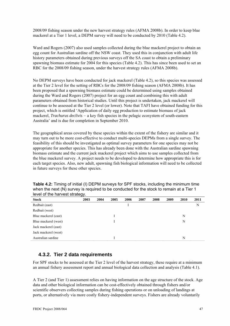
FRDC Project 2008/064 47
2008/09 fishing season under the new harvest strategy rules (AFMA 2008b). In order to keep blue mackerel at a Tier 1 level, a DEPM survey will need to be conducted by 2010 (Table 4.2). Ward and Rogers (2007) also used samples collected during the blue mackerel project to obtain an egg count for Australian sardine off the NSW coast. They used this in conjunction with adult life history parameters obtained during previous surveys off the SA coast to obtain a preliminary spawning biomass estimate for 2004 for this species (Table 4.2). This has since been used to set an RBC for the 2008/09 fishing season, under the harvest strategy rules (AFMA 2008b). No DEPM surveys have been conducted for jack mackerel (Table 4.2), so this species was assessed at the Tier 2 level for the setting of RBCs for the 2008/09 fishing season (AFMA 2008b). It has been proposed that a spawning biomass estimate could be determined using samples obtained during the Ward and Rogers (2007) project for an egg count and combining this with adult parameters obtained from historical studies. Until this project is undertaken, jack mackerel will continue to be assessed at the Tier 2 level (or lower). Note that TAFI have obtained funding for this project, which is entitled ‘Application of daily egg production to estimate biomass of jack mackerel, Trachurus declivis - a key fish species in the pelagic ecosystem of south-eastern Australia’ and is due for completion in September 2010. The geographical areas covered by these species within the extent of the fishery are similar and it may turn out to be more cost-effective to conduct multi-species DEPMs from a single survey. The feasibility of this should be investigated as optimal survey parameters for one species may not be appropriate for another species. This has already been done with the Australian sardine spawning biomass estimate and the current jack mackerel project which aims to use samples collected from the blue mackerel survey. A project needs to be developed to determine how appropriate this is for each target species. Also, new adult, spawning fish biological information will need to be collected in future surveys for these other species.
Table 4.2: Timing of initial (I) DEPM surveys for SPF stocks, including the minimum time when the next (N) survey is required to be conducted for the stock to remain at a Tier 1 level of the harvest strategy. Stock 2003 2004 2005 2006 2007 2008 2009 2010 2011 Redbait (east) I N Redbait (west) Blue mackerel (east) I N Blue mackerel (west) I N Jack mackerel (east) Jack mackerel (west) Australian sardine I N
4.3.2. Tier 2 data requirements For SPF stocks to be assessed at the Tier 2 level of the harvest strategy, these require at a minimum an annual fishery assessment report and annual biological data collection and analysis (Table 4.1). A Tier 2 (and Tier 1) assessment relies on having information on the age structure of the stock. Age data and other biological information can be cost-effectively obtained through fishers and/or scientific observers collecting samples during fishing operations or on unloading of landings at ports, or alternatively via more costly fishery-independent surveys. Fishers are already voluntarily
FRDC Project 2008/064 48
collecting samples of their catch, but it is unknown whether these data collections are useful. A case study for redbait is provided at Appendix H outlining some of the sampling considerations needed to ensure representative samples are collected. The case study provides an example of the necessary information required to determine whether industry-collected samples are sufficient for determining the age structure of a stock and whether there are any changes to that age structure over time.
4.3.3. Tier 3 data requirements For SPF stocks to be assessed at the Tier 3 level of the harvest strategy, these require at a minimum an annual fishery assessment report (Table 4.1). For each tier of the harvest strategy, an annual fishery assessment report is required to provide updated biological information on each of the target species, and catch and effort information over time, which can then be compared with RBCs set for the fishery.
4.4. Discussion A summary of the research plan and associated research and monitoring activities to underpin the SPF Harvest Strategy is provided in Table 4.3. Information is provided on each suggested activity and its relative priority; the specified timeframe in which the activity will need to be undertaken; and the potential research providers and indicative costs for undertaking the research or monitoring activity. SARDI have submitted a research proposal to AFMA, entitled ‘Monitoring and assessment of the Small Pelagic Fishery under the new Harvest Strategy (1 July 2009 to 30 June 2011)’, which has now been approved. This project aims to synthesise catch and effort information and to collect information on the age/size structure of catches of the SPF target stocks. The two analyses combined will meet the minimum requirements for Tier 2, namely a fishery assessment report, and collection and analysis of biological data. Two reports will be produced, the first in April 2010 and the second in April 2011, each in time for the setting of TACs for the fishery in those respective years. It would be expected that this be established as an ongoing monitoring program so that SPF species can continue to be assessed at a Tier 1 or Tier 2 level.

Table 4.3: Summary of 2009/10 research plan to support the SPF Harvest Strategy. Note table lists potential research providers and indicative costs only. NA = timeframe or budget not specified. Research item Timeframe Tier Description Potential provider Indicative cost Priority Conduct DEPM surveys and analysis at least once every five years for each required stock
Redbait – 2011 Blue mackerel – 2010 Jack mackerel – 2009, 2013Australian sardine –2010
1 For a stock to continue to be assessed at Tier 1, DEPM surveys need to be conducted at least once every five years.
Redbait and jack mackerel: TAFI Blue mackerel and Australian sardine: SARDI
Redbait – $155,000; Jack mackerel – NA; Blue mackerel & Australian sardine –$433,000
High – if remain at Tier 1 Low – if move to Tier 2/3
Study to conduct DEPM assessment of jack mackerel from archived samples
NA 1 Surveys have been conducted to collect information on jack mackerel, however, a full DEPM analysis has not been completed. The data has been archived, currently held by TAFI and SARDI, and could be used to determine a spawning biomass estimate.
TAFI $40,000* High – if move to Tier 1 Low – if remain at Tier 2/3
Examine options for multi-species DEPM surveys
NA 1 Costs of conducting DEPM surveys could be reduced if more than one species could be assessed with each survey. The feasibility of this needs to be examined as optimal survey parameters for one species may not be suitable for another.
SARDI TAFI
NA Low
Collection and analysis of length/age data
Annual 2 Establishment of an ongoing monitoring program to collect annual biological data for each stock to provide an indication of their status.
SARDI TAFI
$50,000 High
* Note: Project funded and underway
FRD
C Project 2008/064
49

Research item Timeframe Tier Description Potential provider Indicative cost Priority Study to determine optimal sampling frequency for length/age data and design of appropriate monitoring program
2009 2 Determine the best sampling regime for the fishery. Analysis of fishery collected shot-by-shot data – examine variability to design monitoring program.
BRS SARDI TAFI
NA High
Analysis of industry collected samples, with subsample used for ageing – include costings and program for sample collection, storage and analysis
2009 2 Industry has been collecting samples of their catch on an ad hoc basis. However, the analysis, including ageing of subsamples, and assessment of the usefulness of these data have not been carried out.
BRS SARDI TAFI
NA Medium
Fishery assessment report
Annual 1, 2, 3 Report outlining current status of each stock with respect to catch and effort and biological indicators to provide determine sustainability of current harvest levels.
BRS SARDI TAFI
$30,000 High
FRD
C Project 2008/064
50

FRDC Project 2008/064 51
5. Discussion Commonwealth fisheries have been required to implement harvest strategies in accordance with the recently released Commonwealth Fisheries Harvest Strategy Policy. The policy requires that an MSE be conducted to demonstrate that each harvest strategy is robust to the uncertainty inherent in the assessment and management of the respective fishery. In 2007, AFMA engaged a consultant to review the draft SPF Harvest Strategy (Knuckey et al. 2008) against the Harvest Strategy Policy. In June 2008, the AFMA Board approved the SPF Harvest Strategy. However, further testing of the harvest strategy was required to investigate its robustness under a range of management/harvest scenarios. Our project built on the modelling work done in the Knuckey et al. (2008) review, developing a simple operating model to investigate the impact on the stock of the Tier 1 rules and also to investigate alternative harvest scenarios such as different decay rates. The limited and/or ad hoc nature of current and past data collection and monitoring and specific research programs for the SPF (Chapter 2), while providing some insights to the key parameters used in the MSE to evaluate the SPF Harvest Strategy (Chapter 3), mean conclusions drawn from the MSE should be considered with caution. Furthermore, these limitations emphasise the importance of a structured ongoing monitoring and research program, including the use of purpose-designed stock specific DEPM surveys that will satisfy the requirements of the harvest strategy and the respective tier levels, depending on the target stock and level of catch industry are prepared to accept (Chapter 4). A higher RBC/TAC related to a higher tier (i.e. Tier 1) will also mean greater data and monitoring requirements. Notably, industry have indicated that the SPF is moving towards a Tier 2 level fishery in recognition of their level of investment and relative value of the fishery at present. The MSE results have highlighted the difference between the model calculations of virgin spawning biomass and estimates of spawning biomass from the DEPM surveys. The major contributing factors to this are the values used for natural mortality and the maximum number of recruits and steepness in the stock-recruitment relationship. A preliminary investigation into what values the natural mortality would need to be to obtain the DEPM spawning biomass estimates have been presented in this report, but further research is required to obtain appropriate values for all the parameters identified. There are also uncertainties associated with the DEPM derived spawning biomass estimates. The SPFRAG suggested that these are underestimates of the true spawning biomass for most stocks, with only estimates for the Australian sardine (east) stock closer to reality. For redbait (east) and blue mackerel (east and west) the model estimated virgin spawning biomass is possibly too high as the proportion represented by the DEPM derived estimate is very low (23 percent, 13 percent and 31 percent, respectively), and/or the DEPM biomass estimates were too low with the surveys not fully representing the underlying populations. The model seems to be a good predictor for Australian sardine (east) where the proportion of the DEPM derived spawning biomass is 96 percent of model calculated spawning biomass. Irrespective of initial biomass, most management/harvest scenarios — both base case and sensitivity scenarios — reach equilibrium above B20 after the 30 year simulation period. For the base case scenarios for each tier, all except for redbait east and west for Tier 1 reached a median spawning biomass above B48 in the last year of simulation. The lower 10th percentile spawning biomass in the last year was in all base case scenarios above B20, although the Tier 1 base case scenarios were mostly below B48.

FRDC Project 2008/064 52
The MSE results suggest that the Tier 1 rules for harvesting of the SPF stocks are appropriate, as the model predicts an equilibrium is reached prior to the end of the 30 year simulation period for each stock. The spawning biomass estimates from the DEPM surveys are considered to be underestimates of the true spawning biomass, so determining TACs based on these estimates is conservative. Setting the RBC at a constant 15 percent of spawning biomass for the five years between surveys, as an alternative tier 1 harvest strategy to the current five year decay function in the harvest strategy, had a similar result to the base case scenario but without the cyclical pattern. The risks associated with this alternative harvest strategy for each stock were low, albeit slightly higher than the base cases in both the risk performance statistics used. For redbait (east) and blue mackerel (east and west) where the DEPM estimate of spawning biomass was a low proportion of the model calculated virgin spawning biomass, the Tier 2 and Tier 3 harvest regimes show a significant recovery of the stock to near virgin spawning biomass levels. These results need to be considered with caution. These scenarios use absolute values for catches rather than the relative values (or proportions) used in the Tier 1 scenarios. The proportion of the biomass harvested under a Tier 2 or Tier 3 regime is much smaller if the initial spawning biomass is estimated by the model than by the DEPM surveys, so the impact on the stock is smaller. In conclusion, the MSE results show that the Tier 1 harvest regimes for all stocks, using proportions of the spawning biomass to determine TACs, are sustainable and that an equilibrium is reached by the end of the 30 year simulation period that is well above B20. Similar results were observed for the Tier 2 and Tier 3 harvest regimes, but should be treated with caution as these use absolute values for harvest quantities that may or may not be meaningful for the model calculated spawning biomass estimates. Furthermore, the MSE developed in this project is based on a simple operating model. It is not a full stock assessment model and should not be treated as such. Notably, there is no conditioning of the model on historical catch data from the fishery prior to simulating future stock levels. Adding complexity to the operating model would not necessarily result in an MSE that provides more ‘accurate’ advice, particularly for this fishery with currently limited data about the key input parameters for the target stocks. If the SPF is to move to a Tier 2 fishery, as suggested by industry, the highest priorities for research are (1) an annual fishery assessment report and (2) the ongoing monitoring, collection and analysis of biological data for each stock, including the design of an appropriate monitoring program that determines an optimal sampling regime. These are the minimum requirements for assessment at the Tier 2 level. Harvest strategies for Commonwealth fisheries, as specified under the Harvest Strategy Policy (HSP), should provide a more certain operating environment for industry, while providing the Australian community with confidence that commercial fish species are being managed for long-term biological sustainability and economic profitability. Results from the MSE indicate that current harvest levels specified in the SPF Harvest Strategy are appropriate, where all stocks were maintained at levels well above the default HSP defined biological limit reference point of B20. These results, however, need to be considered in light of the limitations associated with the data inputs and the operating model in the MSE. The MSE provides an initial step to understanding the potential implications of the SPF Harvest Strategy and data gaps that may need to be addressed for the fishery to further develop. The MSE will provide a useful decision-support tool in future reviews of the harvest strategy when new information and data become available.

FRDC Project 2008/064 53
6. Benefits and adoption The main beneficiary of this work will be the SPFRAG, industry and AFMA. The MSE tool has been developed and is available for the SPFRAG to evaluate a range of management/harvest scenarios. The MSE may be used to guide redevelopment of the harvest strategy, providing managers and the community with confidence that fishing will occur at a sustainable rate and providing industry with greater certainty in their operating environment. Sensitivities of the operating model have been tested and the need for better data in some areas has been identified. This will guide research needs into the future. Adoption of results will be through acceptance by SPFMAC and RAG members, with subsequent supporting documentation for the SPF Harvest Strategy provided to the AFMA Commission. The research plan has already been implemented and initiated through a project led by SARDI. This project will involve an analysis of catch and effort data and also collection and analysis of age/size structure of the stocks. This will ensure the SPF stocks reach the minimum data requirements for a Tier 2 assessment.

FRDC Project 2008/064 54
7. Further development Future versions of the MSE would be expected to look at ways to build on what was acknowledged to be a starting point in terms of exploring harvest strategies and species dynamics relating to the SPF. If new data becomes available or further analysis is done, this MSE should be modified to make the best use of additional information. Areas where further development would be beneficial have been identified and include:
• investigating the discrepancy for most stocks between the model calculated virgin spawning biomass and the estimates of spawning biomass from the DEPM surveys. This would include exploring how to best characterise the sampling error inherent in DEPM surveys, as well as justifying parameter values used in the model to calculate the virgin spawning biomass. Of particular importance would be the estimate of the maximum number of recruits which was arbitrarily chosen as 800 million as in Knuckey et al (2008). The interaction between the three parameters with the most uncertainty that effect the estimate of virgin spawning biomass (i.e. steepness, natural mortality and the maximum number of recruits) would be important in getting a better understanding of the model estimated value. Greater agreement between the two estimates of spawning biomass will mean that more confidence can be placed on MSE management scenarios using Tier 2 and Tier 3 harvest regimes (i.e. absolute catches)
• analysis of data and study of relevant literature to get a better understanding of whether
serial correlation in the residuals of the stock-recruitment relationship is required
• exploring the sensitivities of the MSE to uncertainty around selectivities at age, along with further study of the SPF species to better understand behaviour as related to selectivity
• use of smooth selectivity curves in catch curve analysis, and use of catch curve prediction
intervals to determine uncertainty in estimation of selectivity
• analysis of SPF catch and TAC data to better understand the nature of the implementation error included in the model
• if further data becomes available, including from DEPM surveys and fishery catch data, a
more complex statistical model could be justified to provide greater insights into the robustness of the harvest strategy

FRDC Project 2008/064 55
8. Planned outcomes The MSE will provide a useful decision-support tool for the SPFRAG to assess and review the harvest strategy, including alternate management/harvest scenarios. The MSE model code is freely available for others to use, develop further and adopt for other small pelagic fisheries (see Appendix D). The MSE results should provide a level of confidence and/or greater insight to stakeholders on the appropriateness of the current SPF Harvest Strategy, and in relation to current catch levels of SPF stocks. The project has identified data gaps for each SPF stock, including those related to key biological parameters and biomass derived estimates from DEPM surveys, as well as limitations of the MSE model. These will need to be addressed in order to further develop and improve upon the current specifications of the model. The research plan formulated in the project specifies the minimum data and information requirements that are needed to meet the requirements of the SPF Harvest Strategy. This has led to a research project to deliver the requirements for each SPF stock to be maintained at Tier 2 of the harvest strategy.

FRDC Project 2008/064 56
9. Conclusion A new management strategy evaluation (MSE) tool has been developed for the Small Pelagic Fishery (SPF). The sensitivities of the model have been tested, and various harvest strategies explored, as outlined in the SPF Harvest Strategy as well as alternatives to these. The MSE results show that the Tier 1 harvest regimes for all SPF stocks, using proportions of the spawning biomass to determine TACs, are sustainable and that an equilibrium is reached by the end of the 30 year simulation period that is well above B20. Similar results were observed for the Tier 2 and Tier 3 harvest regimes, but these should be treated with caution as these use absolute values for harvest quantities that may or may not be meaningful for the model calculated spawning biomass estimates. A research plan has been developed to underpin the SPF Harvest Strategy and is already being implemented, with two projects obtaining funding. If the SPF is to move to a Tier 2 fishery, as indicated by industry, the research plan indicates that the highest priorities for research are:
1. an annual fishery assessment report 2. the design of an appropriate monitoring program, based on a study that determines an
optimal sampling regime. The research plan is currently being implemented with a project co-ordinated by the South Australian Research and Development Institute (SARDI) to produce a fishery assessment report and collate information on age/size structure of the target stocks. These will meet the minimum requirements for Tier 2 assessments. The Tasmanian Aquaculture and Fisheries Institute (TAFI) have also obtained funding for a project entitled ‘Application of daily egg production to estimate biomass of jack mackerel, Trachurus declivis - a key fish species in the pelagic ecosystem of south-eastern Australia’, which is due for completion in September 2010.

FRDC Project 2008/064 57
10. References AFMA (2008a) Small Pelagic Fishery Harvest Strategy. Australian Fisheries Management
Authority, Canberra. 10pp. AFMA (2008b) Small Pelagic Fishery Resource Assessment Group (SPFRAG): Meeting Record,
Meeting 06, 31 March 2008. Australian Fisheries Management Authority, Canberra. 13pp. http://www.afma.gov.au/fisheries/small_pelagic/rag/default.htm.
Barrowman, N.J., Myers, R.A. (2000) Still more spawner-recruitment curves: the hockey stick and its generalisations. Canadian Journal of Fisheries and Aquatic Sciences, 57: 665-676.
Begg, G.A., O’Neill, M.F, Cadrin, S.X., Bergenius, M.A.J. (2005) Stock assessment of the Australian east coast spotted mackerel fishery. CRC Reef Research Centre Technical Report No. 58, CRC Reef Research Centre, Townsville, Australia.
Browne, A. (2005) Changes in the growth and age structure of jack mackerel in south-east Australian waters. Honours thesis, School of Zoology, Tasmanian Aquaculture and Fisheries Institute, 58pp.
Butterworth, D.S. and Punt, A.E. (1999) Experiences in the evaluation and implementation of management procedures. ICES Journal of Marine Science, 56: 985-998
DAFF (2007) Commonwealth Fisheries Harvest Strategy: Policy and Guidelines. Department of Agriculture, Fisheries and Forestry, Canberra. 63pp.
Dichmont, C.M., Deng, A., Punt, A.E., Ellis, N., Venables, W.N., Kompas, T., Ye, Y., Zhou, S. and Bishop, J. (2008) Beyond biological performance measures in management strategy evaluation: Bringing in economics and the effects of trawling in the benthos. Fisheries Research, 94: 238-250.
Ewing, G. P., and Lyle, J. M. (2009) Reproductive dynamics of redbait, Emmelichthys nitidus (Emmelichthyidae), from south-eastern Australia, Fisheries Research, 97: 206-215.
FAO (1998) Introduction to tropical fish stock assessment. Part 1: Manual. FAO Fisheries Technical Paper 306/1 Rev.2. Food and Agriculture Organization of the United Nations.
Haddon, M. (2001) Modelling and quantitative methods in fisheries. Chapman and Hall, Boca Raton.
Haltuch, M.A., Punt, A,E, and Dorn, M.W. (2008) Evaluating alternative estimators of fishery management reference points. Fisheries Research, 94: 290-303.
Hilborn, R. (1985) Simplified calculation of optimum spawning stock size from Ricker’s stock recruitment curve. Canadian Journal of Fisheries and Aquatic Sciences, 42: 1833-1834.
Hilborn, R. and Walters, C.J. (1992) Quantitative fisheries stock assessment. Choice, dynamics and uncertainty. Chapman and Hall, London.
Hobsbawn, P. and Summerson, R. (2008) Small Pelagics Fishery, in Larcombe, J. and Begg, G. (eds) 2008, Fishery Status Reports 2007: Status of Fish Stocks Managed by the Australian Government, Bureau of Rural Sciences, Canberra, pp. 228-232.
Hoenig, J.M. (1983) Empirical use of longevity data to estimate mortality rates. Fishery Bulletin, 82: 898-903.
Lai, H.L. (1993) Optimal sampling design for using the age-length key to estimate age composition of a fish population Fishery Bulletin, US,92: 382-388.
Kell, L.T., De Oliveira, J.A.A., Punt, A.E., McAllister, M.K. and Kuikka, S. (2006) Operational Management Procedures: an introduction to the use of evaluation frameworks. In, Motos L. and Wilson D.C. (eds.). The Knowledge Base for Fisheries Management, Elsevier, Amsterdam. pp. 379–407.

FRDC Project 2008/064 58
Knuckey, I., Bergh, M., Bodsworth, A., Koopman, M. and Gaylard, J. (2008) Review of the Draft Harvest Strategy for the Commonwealth Small Pelagic Fishery. Australian Fisheries Management Authority and Fishwell Consulting. AFMA Project R2008/843.
Koopman, M.T., Punt, A.E. and Smith, D.C. (2000) Production parameters from the fisheries literature for SEF-like species. Report of ARF Project R99/0308
Kranz, L. (2007) Small Pelagic Fishery: Purse Seine Scientific Observer Manual, Australian Fisheries Management Authority, Canberra.
Myers, R.A. (2001) Stock and recruitment: generalizations about maximum reproductive rate, density dependence, and variability using meta-analytic approaches. ICES Journal of Marine Science, 58: 937-951.
Myers, R.A., Bowen, K.G., and Barrowman, N.J. (1999) Maximum reproductive rate of fish at low population sizes. Canadian Journal of Fisheries and Aquatic Sciences 56: 2404-2419
Neira, F.J., Lyle, J.M., Ewing, G.P., Keane, J.P. and Tracey, S.R. (2008) Evaluation of egg production as a method of estimating spawning biomass of redbait off the east coast of Tasmania. Final Report to Fisheries Research and Development Corporation. FRDC Project No. 2004/039. Fisheries Research and Development Corporation and Tasmanian Aquaculture and Fisheries Institute.
Quinn, T. J., Deriso, R. B. 1999, Quantitative Fish Dynamics, Oxford University Press, New York. Ricker, W. E., 1975, Computation and Interpretation of Biological Statistics of Fish Populations,
Bulletin of the Fisheries Research Board of Canada, Ottawa. Rogers, P.J., Ward, T.M., McLeay, L.J., Lowry, M., Saunders, R.J., and Williams, D. (2009).
Reproductive biology of blue mackerel, Scomber australasicus, off southern and eastern Australia: suitability of the Daily Egg Production Method for stock assessment. Marine and Freshwater Research 60: 187-202.
Smith, P. J, (1989) Is Two-Phase Sampling Really Better for Estimating Age-Composition?, Journal of the American Statistical Association, 84(408): 916-921.
Ward, T.M. and Rogers, P.J. (2007) Development and evaluation of egg-based stock assessment methods for blue mackerel Scomber australasicus in southern Australia. Final Report to Fisheries Research and Development Corporation. FRDC Project 2002/061. Fisheries Research and Development Corporation, NSW Department of Primary Industries, South Australian Research and Development Institute and Tasmanian Aquaculture and Fisheries Institute.
Ward, T.M., Rogers, P.J., McLeay, L.J., and McGarvey, R. (2009). Evaluating the use of the Daily Egg Production Method for stock assessment of blue mackerel, Scomber australasicus. Marine and Freshwater Research 60: 112-128.
Williams, H., Pullen, G, Kucerans, G. and Waterworth, C. (1987) The Jack Mackerel Purse Seine fishery in Tasmania, 1986-87. Technical report 19, Department of Sea Fisheries, Tasmanian marine Laboratories, 32 pp.
Wu, S. (1970) Age and growth of Taiwan spotted mackerel, S. australasicus. M.Sc. Thesis, Dept. of Zoology, National Taiwan University, pp. 38.
Zhou, S. (2007) Discriminating alternative stock-recruitment models and evaluating uncertainty in model structure. Fisheries Research 86: 268-270.

FRDC Project 2008/064 59
Appendix A. Intellectual property No patentable or marketable products or processes have arisen from this research. All results will be published in scientific and non-technical literature. The raw data remains the property of those from which it originated. Intellectual property accruing from the model development and code, analysis and interpretation vests with the Department of Agriculture, Fisheries and Forestry, Bureau of Rural Sciences. The MSE code has been developed for the explicit use of the SPFRAG.

FRDC Project 2008/064 60
Appendix B. Staff Principal Investigator: Patricia I. Hobsbawn Co-Investigators: Fiona Giannini Gavin A. Begg Mark Chambers All staff are from the Department of Agriculture, Fisheries and Forestry, Bureau of Rural Sciences.

FRDC Project 2008/064 61
Appendix C. Small Pelagic Fishery Harvest Strategy (June 2008)
Background The development of the Small Pelagic Fishery (SPF) Harvest Strategy (HS) reflects obligations under the Commonwealth’s Fisheries Harvest Strategy Policy and Guidelines1. The Harvest Strategy Policy (HSP) was developed as a direct response to a Ministerial Direction2 calling for the Australian Fisheries Management Authority (AFMA) to take a more science-based approach to setting total allowable catches and effort in Commonwealth fisheries. Consistent with the HSP, the HS is to provide the Australian community with a high degree of confidence that commercial fish species are being managed for long-term biological sustainability and economic profitability. The HSP provides a framework for Commonwealth HS’s but recognises that it cannot explicitly prescribe the settings for every possible management circumstance. The Policy therefore allows flexibility around the HS design, provided that the strategy delivers the outcomes envisaged by the Policy. Characteristics of the SPF dictate that certain departures from the default HSP standards are required. This SPF harvest strategy is similar to approaches successfully applied in other large fisheries for small pelagic species (e.g. South Australian Sardine Fishery, USA Pacific Sardine Fishery) and has been developed to account for key fishery specific attributes. These are that: • recent catches are limited by economic constraints and are considered by the SPF Resource
Assessment Group (SPFRAG) to be below the maximum sustainable level, and there is potential for sustainable expansion of the fishery;
• the schooling behaviour of all SPF species, combined with main harvesting methods (purse seining and mid water trawling) means that catch per unit effort (CPUE) provides minimal information about stock status;
• given the current information about the fishery; and the potential for large, unpredictable inter-annual variations in availability and/or abundance of small pelagic species; B0 and BMEY are not immediately suitable reference points;
• although small pelagic fishes occur throughout Australian waters, fishing is currently located near processing and transport infrastructure so there is potential for localised depletion;
• small pelagic species are important for both commercial and recreational fisheries; • SPF species are an important food source for many threatened, endangered and protected
species (TEPs) and other species and it is therefore important that the SPF HS takes into account the ecosystem role of these species;
• small pelagic species are caught in high volumes and have low unit value. Additionally, there are high capital costs associated with the large scale catching units and specific processing infrastructure required. As a result, fishing operators need to have heightened efficiency; and
• there are considerable economies of scale in the fishery and the most efficient way to fish may include large scale factory freezer vessels.
1 Commonwealth Fisheries Harvest Strategy Policy and Guidelines, September 2007. by the Minister for Fisheries, Forestry and Conservation. 2 A Direction to issued to AFMA under section 91 of the Fisheries Administration Act 1991 on 14 December 2005 by the Minister for Fisheries, Forestry and Conservation.

FRDC Project 2008/064 62
SPF Harvest Strategy
Objectives Consistent with the HSP, the objective of the SPF HS is: The sustainable and profitable utilisation of the Small Pelagic Fishery in perpetuity through the implementation of a harvest strategy that maintains key commercial stocks at ecologically sustainable levels and, within this context, maximises the net economic returns to the Australian community.
Scope The HSP applies to ‘key commercial species’ in Commonwealth fisheries. For the SPF these species are those that will be subject to quota management under the proposed SPF plan of management (listed below). The SPF HS will apply to the entire area of the fishery (including the existing Zone A) and will be used to develop advice on Recommended Biological Catch (RBC) and Total Allowable Catches (TACs) for all known stocks for each quota species. RBCs derived from the SPF HS will apply to fish stocks throughout their range and to mortality resulting from all types of fishing. The RBCs will be explicitly conservative to account for the ecological importance of these species. Quota species prescribed under the draft SPF plan of management are: • Jack mackerels (Trachurus declivis, and T. murphyi) • Blue mackerel (Scomber australasicus) • Redbait (Emmelichthys nitidus) • Australian sardine (Sardinops sagax) in Commonwealth waters adjacent to NSW
Principles for recommending TACs from RBCs Recommended TAC’s will be calculated by subtracting significant mortality arising from other sources of fishing mortality from the RBCs. Adjustments for catches taken in other fisheries will be based on a five year average of recorded annual catches. It is recognised that in the absence of formal catch sharing arrangements for straddling SPF stocks between state and Commonwealth fisheries, commensurate adjustments to catch limits can not be assured between jurisdictions. SPFMAC considers that catch sharing arrangements should be pursed with the relevant states as a matter of priority to provide certainty of access to SPF resources.
Assessment and monitoring The SPF draft HS is based on a fishery-independent stock assessment technique, known as the Daily Egg Production Method (DEPM). This technique is recognised nationally and internationally as being an effective and cost-efficient method for estimating the spawning biomass of small pelagic fishes. Supporting the DEPM assessment, the SPF HS also relies on continuing monitoring of fishery-dependent data such as catch and effort and size/age catch structure information. Despite the potential biases associated with this data, continuing fishery monitoring was considered to have

FRDC Project 2008/064 63
some potential to be indicative of stock stress, recruitment variability or even changes in fishing practices. The DEPM was developed specifically for small pelagic fishes and explicitly recognises the life history of these species (Lasker 1985). The DEPM provides estimates of spawning biomass that are calculated from information on daily egg production and daily fecundity (Lasker 1985). The spatially explicit nature of the method ensures that stock assessments are stock-based. It is important that the DEPM surveys are conducted over a suitable time period to ensure that spawning times are sampled. If a DEPM survey does not sample the complete range of the stock, the estimate of spawning stock biomass will be more precautionary. The spatial coverage of the surveys can be increased as the fishery expands. In the event that alternative assessment methods are identified and proven to be more cost-effective, the HS may be amended to incorporate decisions rules appropriate for those assessments.
Harvest Strategy Framework The HS is designed to support the orderly development of the fishery and explicitly provides an adaptive management approach that provides for ongoing refinement of the strategy. A tiered HS framework is appropriate for the SPF because it will accommodate growth of the fishery and the consequent collection of additional information to support stock assessment. Underpinning the tiered approach is the need to balance risk with knowledge by establishing exploitation rates that are initially very conservative and which increase (but remain conservative) as additional information (i.e. quantitative measures of spawning biomass) become available. The framework explicitly allows the level of investment research and assessment to be varied to match commercial interest in exploiting the resource. It is understood by SPFRAG and the SPF Management Advisory Committee that assessment costs are likely to increase as the fishery moves towards a Tier one assessment. It is also recognised, however, that an increase in assessment rigor may not necessarily result in a commensurate increase in the RBC. Rather, the RBC will be dictated by the status of the stock. Tiers apply to individual species within a fisheries management unit. The tiers defined in this HS recognise that: • there is a learning phase associated the application of the DEPM to estimate the spawning
biomass of a particular fisheries management unit; • the information that individual estimates of spawning biomass provide on current stock status
decays overtime; • information is needed on the stock status of each fisheries management unit; and • exploitation rates will reflect levels of knowledge about stock status.

FRDC Project 2008/064 64
Decision Rules and reference points The RBC limits and exploitation rates (catch/spawning biomass) assigned in the tiers below were selected on the basis of: i) SPFRAG’s understanding of the status of stocks; ii) previously accepted harvest limits for the fishery; and iii) precautionary harvest rates successfully applied in other fisheries for small pelagic species. The HS reference points are deliberately precautionary to take account of the ecological importance of SPF species as key prey species. By providing for the ecological importance of the species, it is accepted that a lower level of net economic returns than would otherwise be expected by using BMEY as the target reference point will result. Importantly, the exploitation rates applied are maximum limits only. As prescribed in the decision rules, SPFRAG must consider all available information on the status of the stocks when forming its advice on RBCs. Tier 3 Assessment and monitoring An annual review and analysis of fishing activity based on catch and effort data must be conducted to inform the level of fishing that should be permitted. RBC decision rules
1. The RBC for each stock within each management zone will be recommended by SPFRAG based on available information including biology, historical catch and spatial area of zone but may not exceed 500t.
Tier 2 Assessment and monitoring An annual fishery assessment of catch and effort data as well as annual information on the age structure of catch must be conducted to inform the level of fishing that should be permitted. The fishery assessment should aim to determine likelihood of localised depletion or change in the size/age structure of the catch that cannot be adequately explained by reasons other than a decline in abundance. Noting the developing nature of the fishery, the review may also include consideration of the maximum Tier 2 catch limits based on any additional information. RBC decision rules
1. The RBC for each stock within each management zone will be recommended by SPFRAG based on available information including biology, historical catch and spatial area of zone but may not exceed the values (shown in tonnes) listed in the table below.
Species Western zone Eastern zone
Redbait 5,000 5,000 Blue mackerel 6,500 3,000 Jack mackerels 5,000 5,000 Australian sardine N/A 3,000

FRDC Project 2008/064 65
Tier 1 Assessment and monitoring Assessments must be based on a robust spawning biomass estimate derived from DEPM and annual fishery assessments which include catch and effort data and up to date information on the size/age structure of catch. The aim of the annual fishery assessment is to provide supporting advice regarding the level of fishing that should be permitted. RBC decision rules
1. The RBC for each stock within each management zone will be recommended by SPFRAG based on the DEPM assessment and all available information including biology, historical catch and spatial area of zone. The RBC must not exceed levels resulting from relevant harvest rate listed in the table below.
Age of DEPM assessment (years) Maximum harvest rate as a percentage of median spawning biomass estimated from a DEPM assessment
5 10 4 12.5 3 15 ≤2 17.5
2 in 3 OR 3 in 5 20
2. If two successive DEPM assessments produce significantly different spawning
biomass estimates SPFRAG will, on the merit of the assessments and all other supporting information, exercise its judgement on which assessment to use when deciding on an RBC for a particular stock.
NOTE: If the last DEPM assessment is greater than five years old for a particular stock, that stock must be assessed under Tier 3. Metarules General application If a member of the SPFRAG or SPFMAC considers that following the decision rules would not pursue the objectives of the HSP, SPF Harvest Strategy or other policies or legislation relevant to the fishery (e.g. Bycatch Policy, EPBC Act) then that member/party can request the SPFRAG/MAC or AFMA to reconsider the appropriateness of the action prescribed by the decision rules. Any such request must be made in writing to AFMA and be accompanied by supporting documentation. Upon receipt of such a request, the RAG and subsequently the MAC would consider the request and either of these groups or AFMA may seek further information from the party making the request and/or suitable experts before making a decision. Following consideration of the request, it would be open to AFMA to deviate from the decision rule to increase or decrease catch limits and/or set other such measures as it considers necessary to pursue the relevant management objectives.
FRDC Project 2008/064 66
Temporary additional catch allowance Additional catch allowances over and above the harvest limits prescribed in the Tier rules may be considered to support an exploratory fishing and research program. A research program, agreed to by the RAG and MAC, must be developed as part of a fishing plan detailing the proposed fishing activities, prior to the approval of any increase in catch by AFMA. The following information may be collected as part of the research plan: • Length frequency data from each shot • Aging data from across the defined area (for example 500 otoliths per species) • Gonad condition of sub-sample of fish to determine spawning condition • Ad hoc plankton sampling if fish are in spawning condition • Detailed information of the oceanic conditions (depth / water temp, wind, wave moon etc.) • Samples for a concurrent DEPM assessment (spawning adults) The research program must also include a report providing an analysis of the data collected. The RAG may provide guidance on the anticipated costs associated with this analysis and report writing. Accounting for ecological impacts On the basis of all available information including independent observations of the fishery, the potential ecological effects of the SPF will also be considered by SPFRAG when setting RBCs using the following decision rules.
1. If evidence of significant interactions with threatened, endangered or protected species exists, SPFRAG must recommend one or more of the following: • that a program be established to mitigate interactions; and/or • an appropriate reduction in the RBC; and/or • that the stock/s be reduced to a lower level tier (ie with a smaller catch).
2. If there is evidence of localised depletion or change in age/size structure, SPFRAG must recommend one or more of the following: • an appropriate reduction in the RBC; and/or • appropriate spatial or other management measures.
3. If there is evidence of changes in ecosystem function (eg. reduced breeding success of seabirds) occurring as a result of the SPF, SPFRAG must recommend one or more of the following: • an appropriate reduction in the RBC; and/or • appropriate spatial or other management measures; and/or • that a program be established to:
i) assess the potential impacts of the fishery on the ecosystem; ii) investigate potential ecological performance indicators for the fishery;
and iii) report management performance against those indicators.

FRDC Project 2008/064 67
Review The SPF HS will be reviewed within the first 12 months from its commencement and then periodically as required but at least every three years.
References Lasker, R. (1985). An egg production method for estimating spawning biomass of pelagic fish: application to northern anchovy, Engraulis mordax. NOAA Tech. Rep. NMFS, 36: 1 – 99.
Evaluation Against the Commonwealth Harvest Strategy Policy and Guidelines Commonwealth Harvest Strategies must apply minimum standards for reference points and satisfy important design and implementation criteria prescribed under the HS Policy and Guidelines. The justification for how the SPF draft HS complies with these requirements is detailed below.
HSP standards (applicable to each tier) 1. Maintain fish stocks, on average, at a target biomass point (BTarg or proxy) equal to the
stock size required to produce maximum economic yield (BMEY or proxy)3. B0 and BMEY are not suitable reference points for the SPF due to the high inter-annual variations in biomass that are a characteristic of small pelagic fishes. A more suitable approach for small pelagic fishes, which is used in many fisheries around the world, is to set TACs based on conservative estimates of spawning biomass obtained using the DEPM. In a developmental fishery such as the SPF, it is appropriate to set conservative exploitation rates that reflect the size of the stock and the reliability of estimates of spawning biomass. Internationally, exploitation rates of up to 20% are generally considered to be sustainable for many species of pelagic fishes. Hence, setting exploitation rates at 10-20% of the estimate of spawning biomass is an appropriate approach in a developing fishery such as the SPF. It is an approach that has supported the sustainable development of the South Australian Sardine Fishery. The SPF RAG considers that this approach is more conservative than establishing a HS that aims to maintain the biomass at B40. 2. Ensure fish stocks will remain above a biomass level4 where the risk to the stock is
regarded as too high, that is BLIM (or proxy)5 As above. 3. Ensure that stocks stay above the limit biomass level at least 90% of the time.
3 If BMEY is unknown, a proxy of 1.2BMSY (or a level 20% higher than a given proxy for BMSY) is to be used, Where BMSY equals B40. 4 For highly variable species that may naturally breach BLIM, the HS for these species must be consistent with the intent of the Policy. 5 BLIM is equal to or great than 1/2BMSY

FRDC Project 2008/064 68
Limiting the exploitation rate to 10-20% of the estimated spawning biomass will ensure that fishing does not cause the stock to decline to unsustainable levels. As it is not appropriate to estimate B0 for SPF species, it is not suitable to quantify the probability of biomass falling below any limit related to B0. If the SPF RAG agrees that there is evidence of a major decline in stock status that could cause a significant change in ecosystem function, the SPF RAG will consider reducing the TAC reduction. 4. Strategy for rebuilding stocks that are above the limit but below the target reference
points. The SPF is currently considered to under-exploited. The HS for the SPF will prevent overfishing. The highest exploitation rate (20%) of spawning biomass permissible under the SPF HS is conservative. The HS ensures that if biomass declines, catches are reduced accordingly. Experience in the South Australian Sardine Fishery suggests that the approach of setting conservative exploitation rates based on conservative estimates of spawning biomass can also facilitate the recovery of stocks from large declines in biomass that occur as a result of events not related to fishing. This approach allowed the South Australian Sardine Fishery to recover rapidly from two mass mortality events that each killed more than 70% of the adult population. 5. Take into consideration ecosystem interactions. Small pelagic fishes have an important trophic role in marine ecosystems. Managing potential ecosystem impacts is a key element of the HS for the SPF. The exploitation rates are set at a conservative level to explicitly account for these trophic roles, i.e. there is an ‘ecological allocation’ in the HS for the SPF. TACs will also be set for fisheries management units that will be based on the current CSIRO project titled ‘Management zones from small pelagic fish species stock structure in southern Australian waters’. The SPF HS deals directly with the ecological impacts of removing fish from the ecosystem. Harvest Strategies are only one component of AFMA’s overarching framework for achieving Ecosystem Based Fisheries Management. AFMA also conducts Ecological Risk Assessments to identify potential environmental effects, has programs to reduce discards, and has increased fishery independent monitoring.
Harvest strategy design criteria 1. Efficient and cost effective The framework has been designed to explicitly allow the level of investment in research and assessment to be varied to match commercial interest in exploiting the resource. The tiered approach is aimed at allowing investment in stock assessment to be at levels commensurate with the development aspirations of the fishery, and the costs of research are low when catches are low, and costs increase as catches (and risk) increase. Experiences in the South Australian Sardine Fishery show that the DEPM is an effective and efficient approach to assessment of small pelagic fishes. SPFMAC agree however, that further assessment of the HS against this criteria is required and will be addressed through the first 12 month review of the HS. 2. Consistent with Ecologically Sustainable Development (ESD) principles The SPF is HS consistent with ESD principles because it is science based and explicitly precautionary, with low exploitation rates to reflect the ecological importance of SPF species.

FRDC Project 2008/064 69
3. Maximise the net economic returns to the Australian Community The HS is underpinned by an efficient and cost-effective assessment system and provides a framework for the sustainable growth of the SPF where investment in research is matched to commercial interest in exploiting the resource. 4. A high level of transparency in decision making The tiered nature of the HS provides clear decision rules and a transparent framework for decision making. 5. A high level of confidence that objectives will be met The approach has proven effective in similar fisheries. The conservative approach minimises the chance of overfishing. 6. Taking species’ life history into account The HS and assessment technique were developed specifically for small pelagic species (e.g. no attempt to calculate B0 or BMEY).

FRDC Project 2008/064 70
Appendix D. MSE code R version 2.8.0 (2008-10-20) Copyright (C) 2008 The R Foundation for Statistical Computing ISBN 3-900051-07-0 R is a free software environment for statistical computing and graphics. It compiles and runs on a wide variety of UNIX platforms, Windows and MacOS. For details on how to download R, go to http://www.r-project.org/. To run the MSE the following files are required: speciesData.csv (user created file) allSimulations.csv (user created file) runSimulations.r (R code file) modelFunctions.r (R code file) workerFunctions.r (R code file) mainMSE.r (R code file) The two csv files need to be created by the user and the working directories need to be changed at the top of runSimulations.r to the directories where the code has been put, and where the output is to go. Once this is done, running the MSE is done by executing the runSimulations.r script in the R environment. speciesData.csv The speciesData.csv file is a user defined file containing stock dependent information to be used in the MSE. This file can be given any name (e.g. the example file has been given the name redbaitA.csv) but must be provided in the below format (see figure D.1) with the column names as shown.
Column names Description
Age Age class of stock. The last age is a plus group.
Number Numbers of fish in each age class derived from data. These numbers are used in the code as representing relative proportions of fish in age class to the total number of fish.
MortalitiesAtAgea Instantaneous natural mortality for each age.
SelectivityAtAgea The fishing selectivity for each age.
MassAtAgea The weight of a fish at each age.
PropSexMaturity The proportion of sexually mature fish at each age.

FRDC Project 2008/064 71
Figure D.1: Screen shot of an example stock information file. This file is called redbaitA.csv and gives the stock specific information of natural mortality-at-age, selectivity-at-age, mass-at-age and proportion of sexually mature fish-at-age, as well as an age structure defined in terms of numbers of fish in each age class.

FRDC Project 2008/064 72
allSimulations.csv The allSimulations.csv file is a user defined file containing the specification of the scenarios to be run. Each line corresponds to one scenario or set of conditions for a simulation. The file name can not be changed and the format needs to be retained as shown in figure D.2.
Column name Description
Species Name The name of the species for which the scenario is being run. This will appear in generated plots and output files for the run, e.g. Redbait A
Species File The name of the file with the species related data, e.g. redbaitA.csv
No. years Number of years the simulation is to be run over, e.g. 30
No. Repeats The number of repetitions of the scenario to be made, e.g. 1000
Tier Which SPF Harvest Strategy Tier the scenario relates to, e.g. 1
Max. H Prop If a Tier 1 scenario is being simulated, the maximum harvest proportion, e.g. 0.2
Decay If a Tier 1 scenario is being simulated, the decay rate of the harvest proportion, e.g. 0.025
Freq. DEPM If a Tier 1 scenario is being simulated, the frequency of simulated DEPM surveys, e.g. 5 relates to 1 every 5 years.
Survey Biomass SD If a Tier 1 scenario is being simulated, the standard deviation of the error term associated with the simulated DEPM survey, e.g.. 0.3
Max. TAC If a Tier 2 or Tier 3 scenario is being simulated, the maximum TAC in tonnes set for the entire simulation period. If no implementation error is added, this results in a constant catch taken each year of the simulation, e.g. 5000
Implement. Error This value can either be ‘Y’ or ‘N’, corresponding to whether implementation error is to be incorporated in simulation (Y) or not (N).
Alpha The α parameter of the Beta distribution used to incorporate implementation error, e.g. 10
Beta The β parameter of the Beta distribution used to incorporate implementation error, e.g. 1
SR-relationship This value can either be ‘BH’ if a Beverton-Holt stock-recruitment relationship is to be used in the simulation, or ‘HS’ if the Hockey-stick relationship is to be used.
Steepness If a Beverton-Holt stock-recruitment relationship is to be used, the steepness parameter for the particular stock being modelled needs to be given, e.g. 0.74
Kink If a Hockey-stick stock-recruitment relationship is to be used, the percentage of virgin spawning biomass at which the kink in the graph occurs, beyond which maximum recruitment is achieved, e.g. 20 signifies that the kink occurs at 20 percent of virgin spawning biomass.

FRDC Project 2008/064 73
Column name Description
Max. Recruits For both the Beverton-Holt and Hockey-stick stock-recruitment relationships, the maximum number of recruits in millions, e.g. 800 is 800 million recruits.
SD The standard deviation of the recruitment variability term used for both stock-recruitment relationships, e.g. 0.6
serial corr. Used if the recruitment variability term is to incorporate serial correlation, e.g. 0 for no serial correlation, 0.5 for 50 percent correlation.
Use DEPM? This value can either be ‘Y’ if an actual DEPM estimate is to be used as a starting spawning biomass for simulations of ‘N’ if the starting spawning biomass will be some percentage of virgin spawning biomass.
DEPM The actual DEPM estimate in tonnes, e.g. 86990
Age struct This value can be either ‘File’ meaning that the age structure is taken from the Numbers column of the speciesInfo.csv file, or ‘Eq’ if an equilibrium age structure is to be used in simulations.
p If an actual DEPM estimate is to be used as a reference point for the starting spawning biomass in the simulation, then p is the proportion of this estimate to be used as the starting spawning biomass. Else, p corresponds to the proportion of the virgin spawning biomass to be used as the starting spawning biomass, e.g. 0.9 corresponds to starting at 90 percent of the DEPM estimate or the virgin spawning biomass.
Adjust Mortality This can be used to adjust the natural mortality at age provided in the speciesInfo.csv file. If set to 1, the natural mortalities are as given in the file, e.g. 1.2 corresponds to the natural mortalities being increased by 20 percent and 0.8 corresponds to the natural mortalities being decreased by 20 percent.

Figure D.2: Screen shot of the user input file allSimulation.csv. Each line defines the parameters for one scenario run of the SPF MSE.
FRD
C Project 2008/064
74

FRDC Project 2008/064 75
runSimulations.r The code runSimulations.r controls access to the other three R code files. Only this script needs to be run to implement the MSE scenarios defined in the allSimulations.csv file. This code loads into the R environment the functions in workerFunctions.r and modelFunctions.r. It then reads the allSimulations.csv file and sets up the variables used in the model. It creates output files that contain results from all scenarios including a log file that gives the definition of each scenario along with relevant performance statistics. There are two ‘setwd’ lines in the code. The first should be set to the directory where the R code is (i.e. where workerFunctions.r and modelFunctions.r are) and the second should be the directory where the allSimulations.csv file is and where output files are to be put. The ‘source’ line at the bottom of the file should contain the full directory path name of the mainMSE.r file. In runSimulations.r is a variable called ‘burnIn’ that is set to ‘FALSE’ in the code. If this variable is changed to ‘TRUE’, the model will be cycled through for three times the maximum species’ age (without fishing mortality) in order to allow the model to stabilise from the assumed starting conditions before the first year for which there is catch. This is more often done when starting with an equilibrium age structure (see Haltuch et al. 2008). setwd("D:\\Data1\\SPF\\currentCode") source("workerFunctions.r") source("modelFunctions.r") setwd("D:\\Data1\\SPF\\RedbaitA") AllLogFile<<-"allSim_log.csv" allSim<-read.csv("allSimulations.csv", header=T,colClasses = "character") outAllSim<-matrix(nrow=nrow(allSim), ncol=ncol(allSim)+11) colnames(outAllSim)<-c(names(allSim),"Lower End SB","Median End SB","Upper End SB", "Median End 10 SB","Median End 10 SB %","Lower Catch","Median Catch","Upper Catch", "CV Catch", "% Risk 20","Onceoff Risk 20") allMedSpBiomass<-matrix(nrow=nrow(allSim), ncol=30) allMedSpBiomass_rel<-matrix(nrow=nrow(allSim), ncol=30) for(n in 1:nrow(allSim)) { print(n) ######################################################################## #set params speciesName<<-paste(allSim[n,1],n,sep="") print(speciesName) speciesFileName<<-allSim[n,2] if(file.exists(speciesFileName)){

FRDC Project 2008/064 76
speciesInfo<<-read.csv(speciesFileName, header=T) }else{ stop("Species file provided does not exist") } no_Years<<-as.numeric(allSim[n,3]) no_Repetitions<<-as.numeric(allSim[n,4]) whichTier<<-as.numeric(allSim[n,5]) if(whichTier==1){ maxHarvestProp<<-ifelse(is.na(allSim[n,6]),0.2,as.numeric(allSim[n,6])) harvestDecay<<-ifelse(is.na(allSim[n,7]),0.025,as.numeric(allSim[n,7])) DEPM_years<<-ifelse(is.na(allSim[n,8]),"5", allSim[n,8]) DEPM_SD<<-ifelse(is.na(as.numeric(allSim[n,9])),0.3,as.numeric(allSim[n,9])) HarvestProportion<<-calculateHarvestProp(maxHarvestProp,harvestDecay,DEPM_years,no_Years) maxTAC<-NA }else{if(whichTier==2 || whichTier==3){ maxTAC<<-ifelse(is.na(allSim[n,10]),500,as.numeric(allSim[n,10])) maxHarvestProp<-NA harvestDecay<-NA DEPM_years<-NA DEPM_SD<-NA HarvestProportion<-NA }else{ stop("Error: Invalid tier choice") } } implementError<<-ifelse(allSim[n,11] %in% c("Y","y"),1,0) if(implementError){ implementAlpha<<-as.numeric(allSim[n,12]) implementBeta<<-as.numeric(allSim[n,13]) } whichSR<<-allSim[n,14] maxRecruitment<<-as.numeric(allSim[n,17]) recruitment_SD<<-as.numeric(allSim[n,18]) recruitment_corr<<-as.numeric(allSim[n,19]) if(whichSR=="HS"){ recruitment_kink<<-as.numeric(allSim[n,16]) steepness<-NA
FRDC Project 2008/064 77
}else{ steepness<<-as.numeric(allSim[n,15]) recruitment_kink<-NA } useDEPM<<-ifelse(allSim[n,20] %in% c("Y","y"),TRUE,FALSE) if(useDEPM){realDEPM<<-ifelse(is.na(as.numeric(allSim[n,21])),NA,as.numeric(allSim[n,21]))} ageStruct<<-ifelse(is.na(allSim[n,22]),"Eq",allSim[n,22]) startSpBio<<-ifelse(useDEPM==FALSE, "pEquil","pDEPM") p_stSpBio<<-ifelse(is.na(as.numeric(allSim[n,23])),1,as.numeric(allSim[n,23])) adjustMortality<<-ifelse(is.na(as.numeric(allSim[n,24])),1,as.numeric(allSim[n,24])) if(adjustMortality != 1){speciesInfo$MortalitiesAtAgea=speciesInfo$MortalitiesAtAgea*adjustMortality} burnIn<<-FALSE ##################################################################### source('D:\\Data1\\SPF\\currentCode\\mainMSE.r') outAllSim[n,]<-unlist(c(allSim[n,],lowerEndSpBio_percent,medEndSpBio_percent, upperEndSpBio_percent,medEndYearsSpBio,medEndYearsSpBio_percent, lowerCatch,medianCatch,upperCatch,sdCatch/meanCatch,percentRisk_20,onceoffRisk_20)) allMedSpBiomass[n,]<-medSpBiomass allMedSpBiomass_rel[n,]<-medSpBiomass_rel } write.csv(outAllSim, AllLogFile) write.csv(allMedSpBiomass, "allMedSpBiomass.csv") write.csv(allMedSpBiomass_rel, "allMedSpBiomass_rel.csv") modelFunctions.r The modelFunctions.r code contains functions that implement the model equations that have been described in chapter 3. This represents the core of the MSE. These functions are loaded into the R environment by runSimulations.r. PopulationDynamics <- function(SpeciesInfo,SpeciesNumber,FishingPressure,r,currentSpBiomass, BiomassMaxRecruit,maxRecruit,steepness, pristineSpBio,whichSR,

FRDC Project 2008/064 78
recruit_SD) { #Population dynamics equations m<-nrow(SpeciesInfo) NumberAtAgea<-array(dim=m) if(whichSR=="HS"){ NumberAtAgea[1]<-RecruitmentHS(currentSpBiomass,r,BiomassMaxRecruit,maxRecruit,recruit_SD) }else{ NumberAtAgea[1]<-RecruitmentBH(currentSpBiomass,r,steepness,pristineSpBio,maxRecruit,recruit_SD) } NumberAtAgea[m]<-(SpeciesNumber[m-1]*exp(-SpeciesInfo$MortalitiesAtAgea[m-1]*0.5) -FishingPressure*SpeciesNumber[m-1]*exp(-SpeciesInfo$MortalitiesAtAgea[m-1]*0.5)*SpeciesInfo$SelectivityAtAgea[m-1])*exp(-SpeciesInfo$MortalitiesAtAgea[m-1]*0.5)+ (SpeciesNumber[m]*exp(-SpeciesInfo$MortalitiesAtAgea[m]*0.5) -FishingPressure*SpeciesNumber[m]*exp(-SpeciesInfo$MortalitiesAtAgea[m]*0.5)*SpeciesInfo$SelectivityAtAgea[m])*exp(-SpeciesInfo$MortalitiesAtAgea[m]*0.5) for (a in 2:(m-1)) { NumberAtAgea[a]<-(SpeciesNumber[a-1]*exp(-SpeciesInfo$MortalitiesAtAgea[a-1]*0.5) -FishingPressure*SpeciesNumber[a-1]*exp(-SpeciesInfo$MortalitiesAtAgea[a-1]*0.5)*SpeciesInfo$SelectivityAtAgea[a-1])*exp(-SpeciesInfo$MortalitiesAtAgea[a-1]*0.5) } NumberAtAgea[which(NumberAtAgea<0)]=0 return(NumberAtAgea) } TrueSpBiomass <- function(SpeciesInfo, NumberAtAgea) { SpawningBiomassAtAge <- NumberAtAgea * SpeciesInfo$MassAtAgea * SpeciesInfo$PropSexMaturity SpawningBiomass <- sum(SpawningBiomassAtAge) return(SpawningBiomass) } SurveySpBiomassEst <- function(TrueSpawningBiomass, DEPM_SD) { #Spawning biomass estimates from simulated egg production surveys

FRDC Project 2008/064 79
Omega <- rnorm(1,0,DEPM_SD) SurveyBiomass <- TrueSpawningBiomass * exp(Omega) return(SurveyBiomass) } TotalBiomass <- function(SpeciesInfo, NumberAtAgea) { BiomassAtAge <- NumberAtAgea * SpeciesInfo$MassAtAgea TotalBiomass <- sum(BiomassAtAge) return(TotalBiomass) } RecruitmentHS <- function(SpBiomass,r,BiomassMaxRecruit,maxRecruit,recruit_SD) { #HockeyStick Recruitment if (SpBiomass>=BiomassMaxRecruit) { Recruits <- maxRecruit * exp(r-((recruit_SD^2)/2)) } else { Recruits <- maxRecruit * (SpBiomass / BiomassMaxRecruit) * exp(r-((recruit_SD^2)/2)) } return(Recruits) } RecruitmentBH <- function(SpBiomass,r,steepness,pristineSpBio,maxRecruit,recruit_SD) { #BevertonHolt Recruitment numerator=(5*steepness-1)*maxRecruit*SpBiomass denominator=(1-steepness)*pristineSpBio+(5*steepness-1)*SpBiomass Recruits<-(numerator/denominator) * exp(r-((recruit_SD^2)/2)) return(Recruits) } PropAge <- function(SpawningBiomassAtAge, SpawningBiomass) { #Proportions at Age ProportionsAtAge <- SpawningBiomassAtAge/SpawningBiomass return(ProportionsAtAge) }
FRDC Project 2008/064 80
Catches <- function(SpeciesInfo, NumberAtAgea, SurveyBiomass, p, errorAlpha, errorBeta) { #Catches if(SurveyBiomass==0) return(c(0,0,0)) TAC <- p * SurveyBiomass if(errorAlpha==0 && errorBeta==0){ implementationError=1 }else{ implementationError<-rbeta(1,errorAlpha, errorBeta) } Catch <- p * SurveyBiomass * implementationError m<-nrow(SpeciesInfo) weightMidyear<-sqrt(SpeciesInfo$MassAtAgea[1:(m-1)] * SpeciesInfo$MassAtAgea[2:m]) MidyearExBiomass<-sum(NumberAtAgea[-m]*exp(-0.5*SpeciesInfo$MortalitiesAtAgea[-m])* weightMidyear*SpeciesInfo$SelectivityAtAgea[-m])+ (NumberAtAgea[m]*exp(-0.5*SpeciesInfo$MortalitiesAtAgea[m])* SpeciesInfo$MassAtAgea[m]*SpeciesInfo$SelectivityAtAgea[m]) if ((Catch/MidyearExBiomass)<=0.95) { FishingPressure <- Catch/MidyearExBiomass } else { FishingPressure <- 0.95 } RealisedCatch <- FishingPressure * MidyearExBiomass if(RealisedCatch<0){ print(paste("FishingPressure:", FishingPressure)) print(paste("MidyearExBiomass:", MidyearExBiomass )) print(paste("SurveyBiomass:", SurveyBiomass)) print(paste("implementationError:",implementationError) ) } return(c(FishingPressure,RealisedCatch, TAC)) } UnexploitedEquilibrium <- function(SpeciesInfo, MaxRecruits, steepness, maxAge) { #Unexploited equilibrium

FRDC Project 2008/064 81
NumberEqAtAgea<-array(dim=maxAge+1) if(is.na(steepness)){ NumberEqAtAgea[1]<-MaxRecruits #i.e. if SR is Hockey stick }else{ NumberEqAtAgea[1]<- ((5*steepness-1)*MaxRecruits)/(4*steepness) } for (i in 2:(maxAge)) { NumberEqAtAgea[i] <- NumberEqAtAgea[i-1] * exp(-speciesInfo$MortalitiesAtAgea[i-1]) } NumberEqAtAgea[maxAge+1] <- (NumberEqAtAgea[maxAge] * exp(-speciesInfo$MortalitiesAtAgea[maxAge]))/(1-exp(-speciesInfo$MortalitiesAtAgea[maxAge+1])) SpawningBiomassEq <- NumberEqAtAgea* speciesInfo$MassAtAgea * speciesInfo$PropSexMaturity SpawningBiomassEq<-sum(SpawningBiomassEq) BiomassEq <-NumberEqAtAgea* speciesInfo$MassAtAgea BiomassEq <-sum(BiomassEq) return(c(NumberEqAtAgea,SpawningBiomassEq, BiomassEq)) } workerFunctions.r The workerFunctions.r code contains functions that set up data structures for use in implementing the MSE, create and writes initial setup information to a log file, produce plots and generates basic statistics. The last function, rcor, is used to generate the correlated (if required) random normal deviates to be used as the recruitment variability term. Some plots are commented out (which is indicated by the line being preceded by a ‘#’) in order to increase computation time but the comments can be removed if the user wishes to generate those plots. #All these functions are "worker" functions in that they are not part of the model #but set up data for model runs and generate diagnostics from the output of the #model. calculateHarvestProp<-function(maxProp=0.2,decay=0.025, freq="5", years=20){ #constants used in function surveyYears_2in3<-matrix(nrow=3,ncol=3) surveyYears_2in3[1,]<-c(1,0,1) surveyYears_2in3[2,]<-c(1,1,0) surveyYears_2in3[3,]<-c(0,1,1)

FRDC Project 2008/064 82
surveyYears_3in5<-matrix(nrow=9,ncol=5) surveyYears_3in5[1,]<-c(1,1,1,0,0) surveyYears_3in5[2,]<-c(1,1,0,0,1) surveyYears_3in5[3,]<-c(1,1,0,1,0) surveyYears_3in5[4,]<-c(1,0,1,0,1) surveyYears_3in5[5,]<-c(0,0,1,1,1) surveyYears_3in5[6,]<-c(0,1,0,1,1) surveyYears_3in5[7,]<-c(0,1,1,0,1) surveyYears_3in5[8,]<-c(0,1,1,1,0) surveyYears_3in5[9,]<-c(1,0,0,1,1) #start calc decaySeq<-seq(maxProp,maxProp-4*decay,-decay) if(length(grep("2/3",freq))>0){ no_3yr_periods<-ceiling(years/3) randomSurvey<-round(runif(no_3yr_periods,1,3)) surveyYears<<-c(1,as.vector(t(surveyYears_2in3[randomSurvey,])))[1:years] }else { if(length(grep("3/5",freq))>0) { no_5yr_periods<-ceiling(years/5) randomSurvey<-round(runif(no_5yr_periods,1,3)) surveyYears<<-c(1,as.vector(t(surveyYears_3in5[randomSurvey,])))[1:years] }else{ sY<-array(0,dim=years) sY[seq(1,years,as.numeric(freq))]<-1 surveyYears<<-sY }} HProp<-vector(length=years) if(decay==0){ HProp<-rep(maxProp,years) }else{ for(i in 1:years){ if(i==1) HProp[i]<-maxProp-harvestDecay else{ if( (i>1) && sum(surveyYears[c(i-1,i)])==2 ) HProp[i]<-maxProp else{ if( (i>2) && sum(surveyYears[c(i-2,i-1,i)])>1 ) HProp[i]<-maxProp else{ if( (i>3) && sum(surveyYears[c(i-3,i-2,i-1,i)])>2 )HProp[i]<-maxProp else{ if( (i>4) && sum(surveyYears[c(i-4,i-3,i-2,i-1,i)])>2 ) HProp[i]<-maxProp else{ lastSurvey<-max(which(surveyYears[1:i]==1)) surveyAge<-i-lastSurvey+1 if(surveyAge>5)stop("More than 5 years without a survey") if(surveyAge<3) HProp[i]<-decaySeq[2] else{

FRDC Project 2008/064 83
HProp[i]<-decaySeq[surveyAge] } }#end else }#end else }#end else }#end else }#end else }#end for }#end else return(HProp) } writeToLogFile<-function(){ #write to logfile logFileName<<-paste(gsub(" ","_",speciesName),"_log.txt") write("Input values for MSE operating model", logFileName) write(paste("Species: ",speciesName), logFileName,append=T) write("Species data: ", logFileName,append=T) write.table(speciesInfo, logFileName,append=T, quote=F) write(paste("No. of years of simulation: ",no_Years), logFileName,append=T) write(paste("No. of repetitions: ", no_Repetitions), logFileName,append=T) write(paste("Tier",whichTier, "assessment"), logFileName,append=T) if(whichTier==1){ write(paste("DEPM surveys every ", DEPM_years, " years with survey biomass estimate having standard deviation of ", DEPM_SD) , logFileName,append=T) write("Survey years: ", logFileName,append=T) write.table(as.data.frame(surveyYears), logFileName,append=T, quote=F, col.names = F) write("Harvest proportion per year: ", logFileName,append=T) write.table(as.data.frame(HarvestProportion), logFileName,append=T, quote=F, col.names = F) if(useDEPM){write(paste("Using real DEPM estimate of ", realDEPM, "as first survey value"), logFileName, append=T)} }else{ write(paste("Maximum TAC",maxTAC), logFileName,append=T) } if(implementError==1){ write(paste("Implementation error applied to TAC with alpha", implementAlpha, "and beta", implementBeta), logFileName, append=T) }else{ write("No implementation error. i.e. Realised catch = TAC", logFileName, append=T) }

FRDC Project 2008/064 84
if(whichSR=="HS"){ write("Hockey stick stock recruitment relationship used", logFileName, append=T) }else{ write("Beverton-Holt stock recruitment relationship used", logFileName, append=T) } write(paste("Maximum recruitment ", maxRecruitment, " with standard deviation of ", recruitment_SD, "and serial correlation ", recruitment_corr),logFileName,append=T) if(whichSR=="HS"){ write(paste("Hockey stick recruitment has kink at ",recruitment_kink, "% of pristine spawning biomass" ), logFileName,append=T) }else{ write(paste("Beverton-Holt recruitment has a steepness of", steepness), logFileName,append=T) } if(ageStruct=="Eq"){ write("Initial age structure as at equilibrium", logFileName,append=T) }else{ write("Initial age structure as in user provided file", logFileName, append=T) } if(burnIn){write(paste("3 x", nrow(speciesInfo), "years burn in time"), logFileName,append=T)} } setup_dataframes<-function(){ #This function sets up necessary data frames using information read in from the #user yearlyNumbers <- matrix(nrow=nrow(speciesInfo),ncol=no_Years+1, dimnames=list(c(0:(nrow(speciesInfo)-1)), paste(rep("Year",no_Years),0:no_Years, sep=""))) yearlyNumbers[,1]<-speciesInfo$Number yearlyNumbers<<-yearlyNumbers finalNumbers <<- matrix(nrow=nrow(speciesInfo),ncol=no_Repetitions, dimnames=list(c(0:(nrow(speciesInfo)-1)), paste(rep("Simulation",no_Repetitions),1:no_Repetitions, sep=""))) firstName<-paste(rep("Year", (no_Years+1)),0:no_Years, "Age 0") tempNames<-paste(rep("Age",nrow(speciesInfo)*(no_Years+1)), rep(0:(nrow(speciesInfo)-1),no_Years))

FRDC Project 2008/064 85
tempNames[seq(1,nrow(speciesInfo)*(no_Years+1),nrow(speciesInfo))]<-firstName allNumbers <<- matrix(nrow=nrow(speciesInfo)*(no_Years+1),ncol=no_Repetitions, dimnames=list(tempNames, paste(rep("Simulation",no_Repetitions),1:no_Repetitions, sep=""))) catch_ALL <<- matrix(nrow=no_Years,ncol=no_Repetitions, dimnames=list(c(1:no_Years), paste(rep("Simulation",no_Repetitions),1:no_Repetitions, sep=""))) spBiomass_ALL <<- matrix(nrow=no_Years,ncol=no_Repetitions, dimnames=list(c(1:no_Years), paste(rep("Simulation",no_Repetitions),1:no_Repetitions, sep=""))) surveyBiomass_ALL <<- matrix(nrow=no_Years,ncol=no_Repetitions, dimnames=list(c(1:no_Years), paste(rep("Simulation",no_Repetitions),1:no_Repetitions, sep=""))) totalBiomass_ALL <<- matrix(nrow=no_Years,ncol=no_Repetitions, dimnames=list(c(1:no_Years), paste(rep("Simulation",no_Repetitions),1:no_Repetitions, sep=""))) TAC_ALL <<- matrix(nrow=no_Years,ncol=no_Repetitions, dimnames=list(c(1:no_Years), paste(rep("Simulation",no_Repetitions),1:no_Repetitions, sep=""))) risk20 <<- array(0, dim=no_Repetitions, dimnames=list( paste(rep("Simulation",no_Repetitions),1:no_Repetitions, sep="") )) risk30 <<- array(0, dim=no_Repetitions, dimnames=list( paste(rep("Simulation",no_Repetitions),1:no_Repetitions, sep="") )) } generatePlots<-function(){ #This function will generate diagnostic plots and save them to file #relative recruitment of last simulation run #if(yearlyNumbers[1,1]!=0){ # relativeRecruitment<-yearlyNumbers[1,]/yearlyNumbers[1,1] # # plotFileName<-paste(gsub(" ","_",speciesName),"_relRecruit.png") # png(plotFileName) # plot(0:no_Years, relativeRecruitment, xlab="Year",ylab="Relative recruitment", col="red", pch=19)

FRDC Project 2008/064 86
# lines(0:no_Years, relativeRecruitment, col="red") # title("Relative recruitment over simulation period") # dev.off() #} ###relative recruitment using final numbers of all simulation runs #if(finalNumbers[1,1]!=0){ # relativeRecruitment<-finalNumbers[1,]/finalNumbers[1,1] # # plotFileName<-paste(gsub(" ","_",speciesName),"_relRecruitAll.png") # png(plotFileName) # plot(1:no_Repetitions, relativeRecruitment, xlab="Year",ylab="Relative recruitment", col="red", pch=19) # lines(1:no_Repetitions, relativeRecruitment, col="red") # title("Relative recruitment of final year of all simulation runs") # dev.off() #} #median spBiomass + all spBiomass medSpBiomass<<-apply(spBiomass_ALL, 1, median) medSpBiomass_rel<<-medSpBiomass/Ksp maxPlot<-max(spBiomass_ALL)/Ksp minPlot<-min(spBiomass_ALL)/Ksp plotFileName<-paste(gsub(" ","_",speciesName),"_spBiomassAll.png") png(plotFileName) plot(1:no_Years, medSpBiomass_rel, xlab="Year",ylab="Spawning Biomass", ylim= c(minPlot,maxPlot),type="n") for(i in 1:no_Repetitions){ lines(1:no_Years, spBiomass_ALL[,i]/Ksp, lty=2, col="grey") } lines(1:no_Years, medSpBiomass_rel) points(1:no_Years, medSpBiomass_rel, pch=19) title(paste(speciesName, " :relative spawning biomass"), cex=0.75) dev.off() #relative median spBiomass + 90% intervals lowerQuantileSp<-array(dim=no_Years) upperQuantileSp<-array(dim=no_Years) # for(i in 1:no_Years){ # lowerQuantileSp[i]<-quantile(spBiomass_ALL[i,],probs=0.05)

FRDC Project 2008/064 87
# upperQuantileSp[i]<-quantile(spBiomass_ALL[i,],probs=0.95) # } # # lowerQuantileSp_rel<-lowerQuantileSp/Ksp # upperQuantileSp_rel<-upperQuantileSp/Ksp # # maxPlot<-max(upperQuantileSp_rel,1) # # plotFileName<-paste(gsub(" ","_",speciesName),"_spBiomassRel.png") # png(plotFileName) # plot(1:no_Years, medSpBiomass_rel, xlab="Year",ylab="Relative Spawning Biomass", # ylim= c(0,maxPlot),type="l") # points(1:no_Years, medSpBiomass_rel, pch=19) # lines(1:no_Years, lowerQuantileSp_rel, lty="dashed") # lines(1:no_Years, upperQuantileSp_rel, lty="dashed") # # abline(h=0.2,lty=1, lwd=2, col="red") # text(x=2,y=0.23,"20% B0",cex=1) # legend("topright", legend=c("median","lower and upper 5th percentile"),lty=c(1,2)) # # title("Spawning biomass relative to B0") # dev.off() #relative median spBiomass + 80% intervals lowerQuantileSp10<-array(dim=no_Years) upperQuantileSp10<-array(dim=no_Years) for(i in 1:no_Years){ lowerQuantileSp10[i]<-quantile(spBiomass_ALL[i,],probs=0.1) upperQuantileSp10[i]<-quantile(spBiomass_ALL[i,],probs=0.9) } lowerQuantileSp10_rel<-lowerQuantileSp10/Ksp upperQuantileSp10_rel<-upperQuantileSp10/Ksp maxPlot<-max(upperQuantileSp10_rel,1) plotFileName<-paste(gsub(" ","_",speciesName),"_spBiomassRel10.png") png(plotFileName) plot(1:no_Years, medSpBiomass_rel, xlab="Year",ylab="Relative Spawning Biomass", ylim= c(0,maxPlot*1.1),type="l") points(1:no_Years, medSpBiomass_rel, pch=19)

FRDC Project 2008/064 88
lines(1:no_Years, lowerQuantileSp10_rel, lty="dashed") lines(1:no_Years, upperQuantileSp10_rel, lty="dashed") abline(h=0.2,lty=1, lwd=2, col="red") text(x=3,y=0.23,"20% B0",cex=1) legend("topright", legend=c("median","lower and upper 10th percentile"),lty=c(1,2),bty="n") text(x=6,y=maxPlot*1.1,speciesName,cex=1.5) dev.off() #absolute median spBiomass + 80% intervals lowerQuantileSp10<-array(dim=no_Years) upperQuantileSp10<-array(dim=no_Years) for(i in 1:no_Years){ lowerQuantileSp10[i]<-quantile(spBiomass_ALL[i,],probs=0.1) upperQuantileSp10[i]<-quantile(spBiomass_ALL[i,],probs=0.9) } maxPlot<-max(upperQuantileSp10) minPlot<-min(lowerQuantileSp10) plotFileName<-paste(gsub(" ","_",speciesName),"_spBiomass.png") png(plotFileName) plot(1:no_Years, medSpBiomass, xlab="Year",ylab="Spawning Biomass", ylim=c(minPlot,maxPlot*1.1),type="l") points(1:no_Years, medSpBiomass, pch=19) lines(1:no_Years, lowerQuantileSp10, lty="dashed") lines(1:no_Years, upperQuantileSp10, lty="dashed") #abline(h=0.2,lty=1, lwd=2, col="red") #text(x=2,y=0.23,"20% B0",cex=1) legend("topright", legend=c("median","lower and upper 10th percentile"),lty=c(1,2)) title(speciesName, cex=0.75) #title("Spawning biomass over simulation period") dev.off() if(whichTier==1){ #if there is DEPM surveys #median surveyBiomass + all surveyBiomass

FRDC Project 2008/064 89
# medSurveyBiomass<-apply(surveyBiomass_ALL[which(surveyYears==1),], 1, median)/Ksp # # noSurveys<-sum(surveyYears) # maxPlot<-max(surveyBiomass_ALL)/Ksp # minPlot<-min(surveyBiomass_ALL)/Ksp # # plotFileName<-paste(gsub(" ","_",speciesName),"_surveyBiomassAll.png") # png(plotFileName) # plot(1:noSurveys, medSurveyBiomass, xlab="Survey Year",ylab="Spawning Biomass", # ylim= c(minPlot,maxPlot),xaxp=c(1,noSurveys,noSurveys-1), type="n") # for(i in 1:no_Repetitions){ # lines(1:noSurveys, surveyBiomass_ALL[which(surveyYears==1),i]/Ksp, lty=2, col="grey") # } # lines(1:noSurveys, medSurveyBiomass) # points(1:noSurveys, medSurveyBiomass, pch=19) # title("Survey spawning biomass over simulation period for all runs") # dev.off() # #median spBiomass and median survey Biomass with 90% range # lowerQuantileSp<-array(dim=no_Years) # upperQuantileSp<-array(dim=no_Years) # lowerQuantileSur<-array(dim=noSurveys) # upperQuantileSur<-array(dim=noSurveys) # # for(i in 1:no_Years){ # lowerQuantileSp[i]<-quantile(spBiomass_ALL[i,],probs=0.05)/Ksp # upperQuantileSp[i]<-quantile(spBiomass_ALL[i,],probs=0.95)/Ksp # } # # for(i in 1:noSurveys){ # lowerQuantileSur[i]<-quantile(surveyBiomass_ALL[which(surveyYears==1)[i],],probs=0.05)/Ksp # upperQuantileSur[i]<-quantile(surveyBiomass_ALL[which(surveyYears==1)[i],],probs=0.95)/Ksp # } # # maxPlot<-max(upperQuantileSp, upperQuantileSur) # minPlot<-min(lowerQuantileSp, lowerQuantileSur) # # plotFileName<-paste(gsub(" ","_",speciesName),"_biomassQuantilesAll.png") # png(plotFileName) # plot(1:no_Years, medSpBiomass_rel, xlab="Year",ylab="Spawning Biomass", # ylim= c(minPlot,maxPlot),col="red", pch=19) # lines(1:no_Years, medSpBiomass_rel, col="red")

FRDC Project 2008/064 90
# # lines(1:no_Years, lowerQuantileSp, col="red", lty=2) # lines(1:no_Years, upperQuantileSp, col="red", lty=2) # # points(which(surveyYears==1), medSurveyBiomass, pch=19) # # # arrows(x0=which(surveyYears==1), y0=upperQuantileSur, # x1=which(surveyYears==1), y1=lowerQuantileSur, angle=90,code=3,length=0.1) # # legend("topright", legend=c("Actual spawning biomass","Survey spawning biomass"),lty=c(1,1),col=c("red","black")) # title("Actual and survey biomass\n (medians and 90% intervals)") # dev.off() # }#end DEPM plots #median spBiomass and median realised catch with 90% range # lowerQuantileC<-array(dim=no_Years) # upperQuantileC<-array(dim=no_Years) # # lowerQuantileSp<-array(dim=no_Years) # upperQuantileSp<-array(dim=no_Years) # # for(i in 1:no_Years){ # lowerQuantileSp[i]<-quantile(spBiomass_ALL[i,],probs=0.05)/Ksp # upperQuantileSp[i]<-quantile(spBiomass_ALL[i,],probs=0.95)/Ksp # } # # medCatch<-apply(catch_ALL, 1, median)/Ksp # # for(i in 1:no_Years){ # lowerQuantileC[i]<-quantile(catch_ALL[i,],probs=0.05)/Ksp # upperQuantileC[i]<-quantile(catch_ALL[i,],probs=0.95)/Ksp # } # # maxPlot<-max(upperQuantileSp, upperQuantileC) # minPlot<-min(lowerQuantileSp, lowerQuantileC) # # plotFileName<-paste(gsub(" ","_",speciesName),"_spbiomassCatchAll.png") # png(plotFileName) # plot(1:no_Years, medSpBiomass_rel, xlab="Year",ylab="Spawning Biomass", # ylim= c(minPlot,maxPlot),col="red", pch=19)
FRDC Project 2008/064 91
# lines(1:no_Years, medSpBiomass_rel, col="red") # # lines(1:no_Years, lowerQuantileSp, col="red", lty=2) # lines(1:no_Years, upperQuantileSp, col="red", lty=2) # # points(1:no_Years, medCatch, pch=19) # lines(1:no_Years, lowerQuantileC, lty=2) # lines(1:no_Years, upperQuantileC, lty=2) # # title("Spawning biomass and realised catch\n (medians and 90% intervals)") # legend("topright", legend=c("Spawning biomass","Realised catch"),lty=c(1,1),col=c("red","black")) # dev.off() #plots of numbers in age classes #quantNumbers<-matrix(nrow=nrow(allNumbers),ncol=3,dimnames=list(rownames(allNumbers) # ,c("lower","median","upper"))) # for(i in 1:nrow(allNumbers)){ # quantNumbers[i,]<-quantile(allNumbers[i,],probs=c(0.05,0.5,0.95)) # } # # minPlot=min(quantNumbers) # maxPlot=max(quantNumbers) # # plot(0:no_Years, quantNumbers[seq(1,nrow(quantNumbers),nrow(speciesInfo)),2], # ylim=c(minPlot, maxPlot),type="l", ylab="Numbers (in millions)", xlab="Year") # colourRange<-rainbow(nrow(speciesInfo)-1) # for(i in 2:nrow(speciesInfo)){ # lines(0:no_Years, quantNumbers[seq(i,nrow(quantNumbers),nrow(speciesInfo)),2], # col=colourRange[i-1]) # } # } generateStats<-function(){ #mean end spawning biomass as a % of pristine spawning biomass meanEndSpBio<<-mean(spBiomass_ALL[no_Years,]) meanEndSpBio_percent<<-(mean(spBiomass_ALL[no_Years,])/Ksp)*100 #median end sp biomass medEndSpBio<<-median(spBiomass_ALL[no_Years,]) lowerEndSpBio_percent<<-(quantile(spBiomass_ALL[no_Years,],0.1)/Ksp)*100 upperEndSpBio_percent<<-(quantile(spBiomass_ALL[no_Years,],0.9)/Ksp)*100

FRDC Project 2008/064 92
medEndSpBio_percent<<-(median(spBiomass_ALL[no_Years,])/Ksp)*100 #mean sp biomass over last 25% of simulation period end25<-trunc(0.25*no_Years) meanEndYearsSpBio<<-mean(spBiomass_ALL[end25:no_Years,]) meanEndYearsSpBio_percent<<-(meanEndYearsSpBio/Ksp)*100 #median sp biomass over last 10 years medEndYearsSpBio<<-median(spBiomass_ALL[21:no_Years,]) medEndYearsSpBio_percent<<-(medEndYearsSpBio/Ksp)*100 #st. deviation of end spawning biomass for all simulations sdEndSpBio<<-sd(spBiomass_ALL[no_Years,]) cvEndSpBio<<-sdEndSpBio/meanEndSpBio #mean catch meanCatch<<-mean(catch_ALL) sdCatch<<-sd(as.vector(catch_ALL)) medianCatch<<-median(catch_ALL) lowerCatch<<-quantile(catch_ALL,0.1) upperCatch<<-quantile(catch_ALL,0.9) #st. deviation of end spawning biomass for all simulations sdEndSpBio<<-sd(spBiomass_ALL[no_Years,]) cvEndSpBio<<-sdEndSpBio/meanEndSpBio #percentage risk prop of years across all simulations that spbiomass <B20,B30 percentRisk_20<<-(sum(risk20)/(no_Repetitions*no_Years))*100 percentRisk_30<<-(sum(risk30)/(no_Repetitions*no_Years))*100 #Once off risk prop of simulations where at least one year spBiomass <B20,B30 onceoffRisk_20<<-(length(which(risk20>0))/no_Repetitions)*100 onceoffRisk_30<<-(length(which(risk30>0))/no_Repetitions )*100 write("**************************",logFileName,append=T) write(paste("Mean end spawning biomass ", meanEndSpBio),logFileName,append=T) write(paste("As percentage of B0 ", meanEndSpBio_percent, "%"),logFileName,append=T) write(paste("Median end spawning biomass ", medEndSpBio),logFileName,append=T) write(paste("As percentage of B0 ", medEndSpBio_percent, "%"),logFileName,append=T) write(paste("10th percentile end spawning biomass as a percentage of B0 ", lowerEndSpBio_percent, "%"),logFileName,append=T) write(paste("90th percentile end spawning biomass as a percentage of B0 ", upperEndSpBio_percent, "%"),logFileName,append=T) write(paste("Mean spawning biomass of last", end25, "years", meanEndYearsSpBio),logFileName,append=T) write(paste("As percentage of B0 ", meanEndYearsSpBio_percent, "%"),logFileName,append=T)

FRDC Project 2008/064 93
write(paste("Median spawning biomass of last 10 years", medEndYearsSpBio),logFileName,append=T) write(paste("As percentage of B0 ", medEndYearsSpBio_percent, "%"),logFileName,append=T) write(paste("St. Deviation of end spawning biomass ", sdEndSpBio),logFileName,append=T) write(paste("Mean catch ", meanCatch),logFileName,append=T) write(paste("St. Deviation of catch ", sdCatch),logFileName,append=T) write(paste("Median catch ", medianCatch),logFileName,append=T) write(paste("10th percentile catch ", lowerCatch, "%"),logFileName,append=T) write(paste("90th percentile catch ", upperCatch, "%"),logFileName,append=T) write(paste("Percentage risk (Blim) ", percentRisk_20),logFileName,append=T) write(paste("Once-off risk (Blim) ", onceoffRisk_20),logFileName,append=T) write(paste("Percentage risk (B30) ", percentRisk_30),logFileName,append=T) write(paste("Once-off risk (B30) ", onceoffRisk_30),logFileName,append=T) } rcor <- function(n, mu, sigma, rho) { #Generate correlated random Normal deviates result <- 1:n seed <- rnorm(1, mu, sigma) for (i in 1:n) { x <- (seed - mu)/sigma seed <- mu + sigma * (rho * x + rnorm(1) * sqrt(1 - rho*rho)) result[i] <- seed } result } mainMSE.r The mainMSE.r code contains the main loops in the model. The first one loops over the many repetitions to be conducted for a particular scenario and the second loops over the number of years for which each repetition is to be run. Before executing these main loops, some setup in terms of calculating the virgin spawning biomass and setting the required age structure of the stock is done. The mainMSE.r code is called from the runSimulations.r code. writeToLogFile() setup_dataframes() #Find Ksp, number in each age class at equilibrium and the biomass level above which
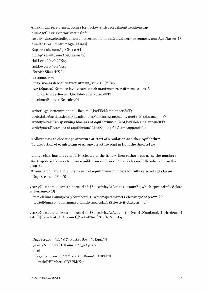
FRDC Project 2008/064 94
#maximum recruitment occurs for hockey stick recruitment relationship numAgeClasses<-nrow(speciesInfo) result<-UnexploitedEquilibrium(speciesInfo, maxRecruitment, steepness, numAgeClasses-1) numEq<-result[1:numAgeClasses] Ksp<-result[numAgeClasses+1] bioEq<-result[numAgeClasses+2] riskLevel20<-0.2*Ksp riskLevel30<-0.3*Ksp if(whichSR=="HS"){ steepness<-0 maxBiomassRecruit<-(recruitment_kink/100)*Ksp write(paste("Biomass level above which maximum recruitment occurs: ", maxBiomassRecruit),logFileName,append=T) }else{maxBiomassRecruit<-0} write("Age structure at equilibrium: ",logFileName,append=T) write.table(as.data.frame(numEq), logFileName,append=T, quote=F,col.names = F) write(paste("Ksp spawning biomass at equilibrium: ",Ksp),logFileName,append=T) write(paste("Biomass at equilibrium: ",bioEq), logFileName,append=T) #Allows user to choose age structure at start of simulation as either equilibrium, #a proportion of equilibrium or an age structure read in from the SpeciesFile #if age class has not been fully selected to the fishery then rather than using the numbers #extrapolated from catch, use equilibrium numbers. For age classes fully selected, use the proportions #from catch data and apply to sum of equilibrium numbers for fully selected age classes if(ageStruct=="File"){ yearlyNumbers[,1][which(speciesInfo$SelectivityAtAgea<1)]=numEq[which(speciesInfo$SelectivityAtAgea<1)] totSelNum<-sum(yearlyNumbers[,1][which(speciesInfo$SelectivityAtAgea==1)]) totSelNumEq<-sum(numEq[which(speciesInfo$SelectivityAtAgea==1)]) yearlyNumbers[,1][which(speciesInfo$SelectivityAtAgea==1)]=(yearlyNumbers[,1][which(speciesInfo$SelectivityAtAgea==1)]/totSelNum)*totSelNumEq } if(ageStruct=="Eq" && startSpBio=="pEquil"){ yearlyNumbers[,1]=numEq*p_stSpBio }else{ if(ageStruct=="Eq" && startSpBio=="pDEPM"){ ratioDEPM<-realDEPM/Ksp

FRDC Project 2008/064 95
write(paste("The real DEPM spawning biomass estimate is ", 100*ratioDEPM, "% of virgin spawning biomass as estimated by the model"),logFileName,append=T) ratiopDEPM<-(p_stSpBio*realDEPM)/Ksp write(paste("Starting spawning biomass is",p_stSpBio , "x DEPM spawning biomass estimate"),logFileName,append=T) write(paste("which is",ratiopDEPM*100 , "% of virgin spawning biomass as estimated by the model"),logFileName,append=T) yearlyNumbers[,1]=numEq*ratiopDEPM }else{ if(ageStruct=="File" && startSpBio=="pEquil"){ totNumbers<-sum(yearlyNumbers[,1]) prop<-yearlyNumbers[,1]/totNumbers newP<-p_stSpBio/(TrueSpBiomass(speciesInfo,prop*sum(numEq))/Ksp) #find the ratio of spawning biomass of age struct from file to virgin sp biomass yearlyNumbers[,1]<-newP*prop*sum(numEq) }else{#File age structure in terms of proportions but starting at biomass as set by DEPM survey ratioDEPM<-realDEPM/Ksp write(paste("The real DEPM spawning biomass estimate is ", 100*ratioDEPM, "% of virgin spawning biomass as estimated by the model"),logFileName,append=T) ratiopDEPM<-(p_stSpBio*realDEPM)/Ksp write(paste("Starting spawning biomass is",p_stSpBio , "x DEPM spawning biomass estimate"),logFileName,append=T) write(paste("which is",ratiopDEPM*100 , "% of virgin spawning biomass as estimated by the model"),logFileName,append=T) totNumbers<-sum(yearlyNumbers[,1]) prop<-yearlyNumbers[,1]/totNumbers newP<-ratiopDEPM/(TrueSpBiomass(speciesInfo,prop*sum(numEq))/Ksp) yearlyNumbers[,1]<-newP*prop*sum(numEq) } } } write("Initial age structure: ",logFileName,append=T) write.table(as.data.frame(yearlyNumbers[,1]), logFileName,append=T, quote=F,col.names = F) #start repetitions for (j in 1:no_Repetitions) { #ouput to log write("**************************",logFileName,append=T) write(paste("Simulation ", j), logFileName,append=T)

FRDC Project 2008/064 96
RecruitmentFactor <- rcor(no_Years, 0, recruitment_SD, recruitment_corr) allNumbers[1:nrow(speciesInfo),j] <- yearlyNumbers[,1] #ouput to log write("Recruitment stochastic component:",logFileName,append=T) write(RecruitmentFactor, logFileName,append=T) #optional "burn in" time if(burnIn==TRUE){ RecruitmentFactor <- rcor(3*nrow(speciesInfo)+no_Years, 0, recruitment_SD, recruitment_corr) for(i in 1:(3*nrow(speciesInfo))){ currentSpBiomass<-TrueSpBiomass(speciesInfo, yearlyNumbers[,1]) yearlyNumbers[,1] <- PopulationDynamics(speciesInfo,yearlyNumbers[,1], 0,RecruitmentFactor[i], currentSpBiomass,maxBiomassRecruit, maxRecruitment,steepness,Ksp,whichSR, recruitment_SD) } print(paste("Burn in time:", i)) write("Age structure after burn in: ",logFileName,append=T) write.table(as.data.frame(yearlyNumbers[,1]), logFileName,append=T, quote=F,col.names = F) } for (i in 1:(no_Years)) { currentSpBiomass<-TrueSpBiomass(speciesInfo, yearlyNumbers[,i]) spBiomass_ALL[i,j]<-currentSpBiomass currentTotalBiomass<-TotalBiomass(speciesInfo, yearlyNumbers[,i]) totalBiomass_ALL[i,j]<-currentTotalBiomass if(currentSpBiomass<riskLevel20){risk20[j]<-risk20[j]+1} if(currentSpBiomass<riskLevel30){risk30[j]<-risk30[j]+1} #ouput to log write(paste("Year ", i), logFileName,append=T) write(paste("True spawning biomass ", currentSpBiomass),logFileName,append=T) write(paste("As percentage of B0 ", (currentSpBiomass/Ksp)*100),logFileName,append=T) if (whichTier==1){ if(surveyYears[i]){ if(i==1 && useDEPM && burnIn==FALSE){

FRDC Project 2008/064 97
SurveyBiomass<-realDEPM write(paste("Real DEPM survey used this year with a survey biomass estimate of ",SurveyBiomass),logFileName,append=T) }else{ SurveyBiomass<-SurveySpBiomassEst(currentSpBiomass, DEPM_SD) write(paste("DEPM survey available this year with a survey biomass estimate of ",SurveyBiomass),logFileName,append=T) } } }else{ SurveyBiomass<-currentSpBiomass } surveyBiomass_ALL[i,j]<-SurveyBiomass if(whichTier==1){ if(implementError){ result <- Catches(speciesInfo,yearlyNumbers[,i],SurveyBiomass, HarvestProportion[i], implementAlpha, implementBeta) }else{ result <- Catches(speciesInfo,yearlyNumbers[,i],SurveyBiomass, HarvestProportion[i], 0, 0) } }else{if(whichTier==2 || whichTier==3){ if(implementError){ result <- Catches(speciesInfo,yearlyNumbers[,i],maxTAC,1, implementAlpha, implementBeta) }else{ result <- Catches(speciesInfo,yearlyNumbers[,i],maxTAC,1, 0, 0) } }else{stop("Error: Invalid Tier")}} FishingPressure <- result[1] catch_ALL[i,j] <- result[2] TAC_ALL[i,j] <- result[3] yearlyNumbers[,i+1] <- PopulationDynamics(speciesInfo,yearlyNumbers[,i], FishingPressure,RecruitmentFactor[i], currentSpBiomass,maxBiomassRecruit, maxRecruitment,steepness,Ksp,whichSR, recruitment_SD) if(any(yearlyNumbers[,i+1]==0)){ write("Some age classes have been fully depleted: ",logFileName,append=T) write.table(as.data.frame(yearlyNumbers[,i+1]), logFileName,append=T, quote=F,col.names = F)
FRDC Project 2008/064 98
} allNumbers[((i*nrow(speciesInfo)+1):((i+1)*nrow(speciesInfo))),j] <- yearlyNumbers[,i+1] }#end for i finalNumbers[,j] <- yearlyNumbers[,(no_Years+1)] #should set up in setup_dataframes }#end for j #write.csv(catch_ALL,paste(gsub(" ","_",speciesName),"_catch.csv")) #write.csv(TAC_ALL,paste(gsub(" ","_",speciesName),"_TAC.csv")) #write.csv(surveyBiomass_ALL,paste(gsub(" ","_",speciesName),"_surveyBiomass.csv")) write.csv(spBiomass_ALL,paste(gsub(" ","_",speciesName),"_spBiomass.csv")) #write.csv(totalBiomass_ALL,paste(gsub(" ","_",speciesName),"_totBiomass.csv")) #write.csv(finalNumbers,paste(gsub(" ","_",speciesName),"_finalNumbers.csv")) write.csv(allNumbers,paste(gsub(" ","_",speciesName),"_allNumbers.csv")) generatePlots() generateStats() Output The result of running the MSE code is the production of many files. If it is not necessary to produce all output, the lines of code that write particular data to file can be commented out (this will also save computation time). The following output files give information on the full set of simulations run (as indicated by the allSimulations.csv file): allMedSpBiomass.csv : Contains the median spawning biomass (of all repetitions) in tonnes for each year of each scenario (i.e. no. of scenarios x no. years). allMedSpBiomass_rel.csv : Contains the median spawning biomass(of all repetitions) relative to virgin spawning biomass for each years of each scenario (i.e. no. of scenarios x no. years). allSim_log.csv : Contains performance statistics for each scenario. The definition of each scenario (as shown in allSimulations.csv) precedes the performance statistics for that scenario. The performance statistics given are
• the lower 10th percentile, median and upper 10th percentile of the spawning biomass in the last year of simulation over all repetitions (given as a percentage of virgin spawning biomass),
• the median spawning biomass for the last 10 years of simulation over all repetitions in tonnes and as a percentage of virgin spawning biomass,
• the lower 10th percentile, median and upper 10th percentile of catch in tonnes over all years and all repetitions,
• the CV of catch over all years and all repetitions, • the percentage risk and the once-off risk.
The second set of files are produced for each scenario. These files will be numbered according to the line number the definition of the scenario occurs in the file allSimulations.csv. The name given in the ‘Species Name’ column of the allSimulation.csv file will be used in naming output for the scenario. The following files produced for each scenario are:
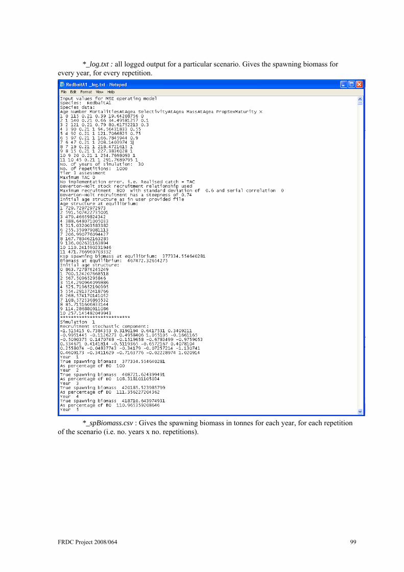
FRDC Project 2008/064 99
*_log.txt : all logged output for a particular scenario. Gives the spawning biomass for every year, for every repetition.
*_spBiomass.csv : Gives the spawning biomass in tonnes for each year, for each repetition of the scenario (i.e. no. years x no. repetitions).

FRDC Project 2008/064 100
*_spBiomass.png: A plot of the median, lower 10th percentile and upper 10th percentile of the spawning biomass in tonnes over all repetitions for each year.
*_spBiomassRel10.png: A plot of the median, lower 10th percentile and upper 10th percentile of the spawning biomass, relative to the virgin spawning biomass, over all repetitions for each year.

FRDC Project 2008/064 101
*_spBiomassAll.png: A plot of the median spawning biomass relative to virgin spawning biomass for all years over all repetitions (the bold line), with the grey lines showing the relative spawning biomass for all, 1000 in this case, repetitions for each year.
*_allNumbers.csv : The numbers of fish (in millions) in each age group for each year of every repetition (i.e. (no. age groups x no. years) x no. repetitions). *_catch.csv : The realised catch in tonnes for each year of every repetition (i.e. no. years x no. repetitions). *_TAC.csv : The TAC in tonnes for each year of every repetition (i.e. no. years x no. repetitions). *_surveyBiomass.csv : The simulated survey biomass for each year of every repetition (i.e. no. years x no. repetitions). *_totBiomass.csv : The total biomass in tonnes for each year of every repetition (i.e. no. years x no. repetitions). *_finalNumbers.csv The number of fish (in millions) in each age group for the last year of each repetition (i.e. no. age groups x no. repetitions). The last five output files (*_catch.csv, *_TAC.csv, *_surveyBiomass.csv, *_totBiomass.csv and *_finalNumbers.csv) are currently commented out in the code to save computation time and space. If these are required, the comment character (‘#’) can be removed from in front of each of the lines of code writing the information to these files.

Appendix E. MSE sensitivity analysis Following are the results of scenario runs for each of the six stocks and the case study.
Redbait A (east) Redbait A End spawning biomass (% of B0) Catch (tonnes) Catch CV % Risk B20 Once-off Risk B20
Scenario Lower Median Upper Lower Median Upper 1 No harvest 77.90 97.12 123.83 0.00 0.00 0.00 0.00 0.00 0.00
Tier 1 2 Base 24.85 39.63 59.07 10885.40 23689.10 49512.93 0.60 2.65 18.90 3 h=0.89 29.25 43.56 62.66 12801.53 26697.19 53239.94 0.56 1.97 16.00 4 h=0.59 19.94 32.91 50.39 8492.41 19600.56 43475.99 0.64 6.64 31.60 5 SRvari=0.3 30.08 41.44 52.34 11803.11 24074.84 48182.17 0.56 1.42 11.40 6 freq=1/2 23.34 33.20 46.38 13797.59 25808.24 51373.28 0.54 1.83 16.70 7 survari=0.6 11.81 34.82 59.61 3710.31 20171.72 59716.47 0.97 19.39 63.10 8 Srcorr=0.5 20.62 38.40 64.91 9767.30 23355.21 50979.09 0.64 6.16 35.10 9 Bstart=100% 25.10 39.70 57.72 11113.49 24622.73 53020.12 0.61 2.93 20.10
10 Bstart=70% 25.54 39.71 58.59 10744.98 22170.89 42548.82 0.53 2.29 17.60 11 Bstart=50% 26.32 39.60 57.18 10369.28 20363.07 36695.16 0.50 2.76 21.00 12 Bstart=86990 26.02 40.39 59.23 8252.33 15044.77 31386.61 0.57 9.79 78.50 13 Bstart=86990, m=0.25 30.57 45.65 65.25 7363.74 13354.63 25684.01 0.53 1.03 9.80 14 Bstart=86990, m=0.17 21.89 34.32 48.82 8795.65 17578.52 38804.30 0.61 30.56 100.00 15 ierror=N 23.47 37.09 54.28 11005.21 24391.74 51805.95 0.61 4.59 28.80 16 Astart=equil 25.59 39.66 56.91 10610.57 22783.64 46865.99 0.59 2.85 19.00 17 m=0.25 29.61 44.49 63.91 8699.10 17981.42 35330.42 0.55 1.23 10.40 18 m=0.17 20.61 33.94 49.13 14043.39 32671.35 72119.81 0.63 5.88 32.00 19 ierror=N, bias=50% 20.37 29.02 42.39 14346.87 25243.98 62669.36 0.61 7.60 46.30 20 maxHProp=0.15, decay=0 25.85 40.25 58.20 11691.70 24257.57 48877.22 0.56 3.22 23.00 21 maxHProp=0.075, decay=0 45.18 60.76 82.99 10304.96 17775.60 29046.29 0.41 0.00 0.00
FRD
C Project 2008/064
102
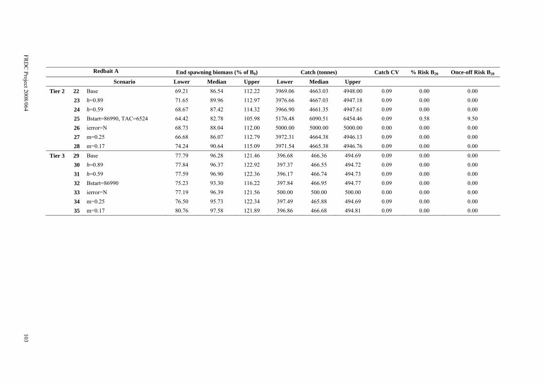
Redbait A End spawning biomass (% of B0) Catch (tonnes) Catch CV % Risk B20 Once-off Risk B20
Scenario Lower Median Upper Lower Median Upper Tier 2 22 Base 69.21 86.54 112.22 3969.06 4663.03 4948.00 0.09 0.00 0.00
23 h=0.89 71.65 89.96 112.97 3976.66 4667.03 4947.18 0.09 0.00 0.00 24 h=0.59 68.67 87.42 114.32 3966.90 4661.35 4947.61 0.09 0.00 0.00 25 Bstart=86990, TAC=6524 64.42 82.78 105.98 5176.48 6090.51 6454.46 0.09 0.58 9.50 26 ierror=N 68.73 88.04 112.00 5000.00 5000.00 5000.00 0.00 0.00 0.00 27 m=0.25 66.68 86.07 112.79 3972.31 4664.38 4946.13 0.09 0.00 0.00 28 m=0.17 74.24 90.64 115.09 3971.54 4665.38 4946.76 0.09 0.00 0.00
Tier 3 29 Base 77.79 96.28 121.46 396.68 466.36 494.69 0.09 0.00 0.00 30 h=0.89 77.84 96.37 122.92 397.37 466.55 494.72 0.09 0.00 0.00 31 h=0.59 77.59 96.90 122.36 396.17 466.74 494.73 0.09 0.00 0.00 32 Bstart=86990 75.23 93.30 116.22 397.84 466.95 494.77 0.09 0.00 0.00 33 ierror=N 77.19 96.39 121.56 500.00 500.00 500.00 0.00 0.00 0.00 34 m=0.25 76.50 95.73 122.34 397.49 465.88 494.69 0.09 0.00 0.00 35 m=0.17 80.76 97.58 121.89 396.86 466.68 494.81 0.09 0.00 0.00
FRD
C Project 2008/064
103

FRD
C Project 2008/064
104

FRD
C Project 2008/064
105

FRD
C Project 2008/064
106

FRD
C Project 2008/064
107

FRD
C Project 2008/064
108

Redbait B (west) Redbait B End spawning biomass (% of B0) Catch (tonnes) Catch CV % Risk B20 Once-off Risk B20
Scenario Lower Median Upper Lower Median Upper 1 No harvest 78.92 98.22 123.05 0.00 0.00 0.00 0.00 0.00 0.00
Tier 1 2 Base 29.86 44.49 62.39 14155.66 29018.35 55361.76 0.53 0.67 7.00 3 h=0.89 33.09 48.61 67.80 15830.51 31690.58 61093.76 0.53 0.72 8.10 4 h=0.59 24.62 38.45 55.60 11364.55 24225.10 49504.57 0.58 2.06 14.40 5 SRvari=0.3 34.91 46.51 57.93 15272.48 29187.88 54759.64 0.51 0.43 4.80 6 freq=1/2 27.36 38.64 54.10 17411.38 31747.70 59248.96 0.49 0.46 6.20 7 survari=0.6 18.41 42.02 64.15 7310.34 25986.13 69255.50 0.85 9.96 52.00 8 Srcorr=0.5 24.10 41.66 69.63 12495.20 28552.24 58307.15 0.59 3.37 23.60 9 Bstart=100% 30.04 44.73 62.76 14115.12 29544.87 59396.50 0.57 1.01 9.90
10 Bstart=70% 29.72 44.46 63.19 13599.07 26908.83 49790.76 0.51 1.06 8.70 11 Bstart=50% 30.27 45.61 64.59 12918.03 24283.79 43430.64 0.48 1.23 11.20 12 ierror=N 27.17 41.65 60.28 14596.35 30083.42 59765.86 0.55 1.82 15.60 13 Astart=equil 30.73 45.17 64.64 13507.92 27562.14 54592.40 0.55 1.25 11.60 14 m=0.25 34.15 50.28 72.63 10863.16 21740.54 40942.39 0.52 0.53 6.30 15 m=0.17 25.05 38.49 55.90 18091.26 38627.47 80035.89 0.59 2.48 18.70 16 ierror=N, bias=50% 23.76 33.77 47.73 18826.66 32405.77 68916.05 0.52 1.94 16.30 17 maxHProp=0.15, decay=0 29.93 45.21 63.07 14914.86 29456.40 55480.49 0.51 1.03 10.80 18 maxHProp=0.075, decay=0 47.67 64.14 84.93 11972.66 20235.79 32776.21 0.39 0.00 0.00
FRD
C Project 2008/064
109

Redbait B End spawning biomass (% of B0) Catch (tonnes) Catch CV % Risk B20 Once-off Risk B20
Scenario Lower Median Upper Lower Median Upper Tier 2 19 Base 71.35 89.77 115.73 3978.56 4668.04 4946.97 0.09 0.00 0.00
20 h=0.89 71.76 91.43 117.55 3979.34 4670.93 4948.83 0.09 0.00 0.00 21 h=0.59 70.56 89.52 113.71 3984.45 4663.99 4945.96 0.09 0.00 0.00 22 TAC=6524 2.27 23.12 48.68 30941.06 37870.63 40290.12 0.14 13.00 49.40 23 ierror=N 72.34 90.46 115.18 5000.00 5000.00 5000.00 0.00 0.00 0.00 24 m=0.25 69.63 88.61 114.59 3970.56 4664.66 4947.67 0.09 0.00 0.00 25 m=0.17 75.17 92.81 115.68 3974.19 4664.71 4947.68 0.09 0.00 0.00
Tier 3 26 Base 80.48 97.71 121.30 398.26 466.66 494.89 0.09 0.00 0.00 27 h=0.89 78.04 96.17 121.82 398.16 466.64 494.76 0.09 0.00 0.00 28 h=0.59 79.20 97.85 123.63 397.04 466.52 494.72 0.09 0.00 0.00 29 ierror=N 79.80 97.59 123.29 500.00 500.00 500.00 0.00 0.00 0.00 30 m=0.25 77.09 96.63 122.35 396.02 466.14 494.83 0.09 0.00 0.00 31 m=0.17 80.74 97.38 120.25 398.24 467.06 494.92 0.09 0.00 0.00
FRD
C Project 2008/064
110

FRD
C Project 2008/064
111

FRD
C Project 2008/064
112

FRD
C Project 2008/064
113

FRD
C Project 2008/064
114
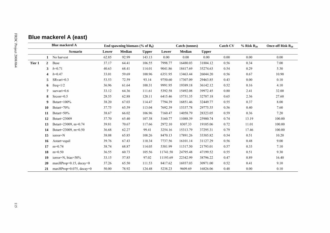
Blue mackerel A (east) Blue mackerel A End spawning biomass (% of B0) Catch (tonnes) Catch CV % Risk B20 Once-off Risk B20
Scenario Lower Median Upper Lower Median Upper 1 No harvest 62.85 92.99 143.13 0.00 0.00 0.00 0.00 0.00 0.00
Tier 1 2 Base 37.17 64.41 106.55 7998.77 16480.03 31804.12 0.56 0.34 7.00 3 h=0.71 40.63 68.41 114.01 9041.86 18417.69 35274.63 0.54 0.29 5.30 4 h=0.47 33.01 59.69 100.96 6351.95 13463.44 26044.20 0.56 0.67 10.90 5 SRvari=0.3 53.53 72.59 93.14 9750.60 17307.09 29463.85 0.43 0.00 0.10 6 freq=1/2 36.96 61.64 100.31 9991.95 19389.18 36142.12 0.52 0.16 4.10 7 survari=0.6 33.12 64.36 111.61 5392.58 15492.08 39972.45 0.80 2.41 32.00 8 Srcorr=0.5 28.55 62.88 120.11 6415.46 15731.35 32787.18 0.65 2.36 27.60 9 Bstart=100% 38.20 67.03 114.47 7794.39 16851.46 32449.77 0.55 0.37 8.00
10 Bstart=70% 37.75 65.59 113.04 7692.39 15337.78 29775.55 0.56 0.40 7.60 11 Bstart=50% 38.67 66.02 106.96 7160.47 14058.79 28323.05 0.59 0.36 7.20 12 Bstart=23009 37.70 65.40 107.38 3160.77 11088.39 25900.74 0.74 13.19 100.00 13 Bstart=23009, m=0.74 39.81 70.67 117.66 2972.10 8307.33 19105.06 0.72 11.01 100.00 14 Bstart=23009, m=0.50 36.68 62.27 99.41 3254.16 15313.79 37295.31 0.79 17.46 100.00 15 ierror=N 38.08 65.85 108.26 8470.13 17891.26 33385.82 0.54 0.51 10.20 16 Astart=equil 39.76 67.43 110.34 7737.56 16101.14 31127.29 0.56 0.48 9.00 17 m=0.74 38.74 68.87 114.05 5381.99 11317.50 21793.01 0.57 0.33 7.10 18 m=0.50 36.55 60.73 105.56 11741.58 24795.48 47199.52 0.55 0.51 9.30 19 ierror=N, bias=50% 33.15 57.85 97.02 11193.69 22342.99 38796.22 0.47 0.89 16.40 20 maxHProp=0.15, decay=0 37.26 65.50 111.53 8417.62 16937.03 30971.00 0.52 0.41 9.10 21 maxHProp=0.075, decay=0 50.00 78.92 124.48 5238.23 9609.69 16826.06 0.48 0.00 0.10
FRD
C Project 2008/064
115

Blue mackerel A End spawning biomass (% of B0) Catch (tonnes) Catch CV % Risk B20 Once-off Risk B20
Scenario Lower Median Upper Lower Median Upper Tier 2 22 Base 58.78 89.55 135.65 2377.60 2798.91 2967.81 0.09 0.00 0.00
23 h=0.71 59.10 87.59 142.11 2390.48 2799.58 2968.28 0.09 0.00 0.00 24 h=0.47 56.33 84.05 137.11 2385.03 2799.07 2968.82 0.09 0.00 0.00 25 Bstart=23009, TAC=1726 59.90 89.07 134.53 1369.34 1610.55 1707.67 0.09 12.59 100.00 26 ierror=N 59.83 87.53 132.97 3000.00 3000.00 3000.00 0.00 0.00 0.00 27 m=0.74 55.43 87.15 141.14 2375.99 2799.28 2968.22 0.09 0.00 0.00 28 m=0.50 61.68 91.23 130.90 2380.68 2798.14 2967.55 0.09 0.00 0.00
Tier 3 29 Base 61.58 93.38 138.63 398.78 466.48 494.61 0.09 0.00 0.00 30 h=0.71 63.33 94.16 136.59 397.37 466.71 494.74 0.09 0.00 0.00 31 h=0.47 59.59 88.91 138.79 397.65 466.41 494.71 0.09 0.00 0.00 32 Bstart=23009 62.60 90.69 138.44 397.24 466.68 494.74 0.09 11.93 100.00 33 ierror=N 61.03 91.88 140.08 500.00 500.00 500.00 0.00 0.00 0.00 34 m=0.74 60.74 91.53 144.15 398.36 466.34 494.62 0.09 0.00 0.00 35 m=0.47 65.90 94.58 138.92 396.31 466.80 494.94 0.09 0.00 0.00
FRD
C Project 2008/064
116

FRD
C Project 2008/064
117

FRD
C Project 2008/064
118

FRD
C Project 2008/064
119

FRD
C Project 2008/064
120

FRD
C Project 2008/064
121

Blue mackerel B (west) Blue mackerel B End spawning biomass (% of B0) Catch (tonnes) Catch CV % Risk B20 Once-off Risk B20
Scenario Lower Median Upper Lower Median Upper 1 No harvest 63.53 94.59 139.20 0.00 0.00 0.00 0.00 0.00 0.00
Tier 1 2 Base 39.46 67.57 112.25 8213.75 17178.27 32922.46 0.54 0.26 5.40 3 h=0.71 43.05 70.25 112.73 9456.35 19134.02 36031.20 0.55 0.27 6.10 4 h=0.47 34.03 59.56 99.64 6612.84 14237.73 27384.10 0.55 0.56 9.10 5 SRvari=0.3 55.26 73.99 93.96 10247.10 18198.38 31009.60 0.43 0.01 0.20 6 freq=1/2 38.54 60.57 101.28 10484.77 20038.68 36430.29 0.51 0.18 4.80 7 survari=0.6 32.58 63.88 110.30 5625.99 15845.38 41440.67 0.80 2.14 30.90 8 Srcorr=0.5 27.07 60.78 117.89 6737.80 16483.32 34310.05 0.65 2.15 25.40 9 Bstart=100% 37.96 67.19 111.20 8230.78 17593.89 34338.47 0.56 0.36 7.80
10 Bstart=70% 38.46 67.37 107.33 7996.42 16120.80 30994.05 0.56 0.34 6.90 11 Bstart=50% 38.41 65.40 111.30 7293.63 14661.46 29799.65 0.59 0.39 8.70 12 Bstart=56288 37.74 66.37 110.71 6272.21 12986.36 28506.97 0.65 0.57 12.40 13 Bstart=56288, m=0.74 39.53 70.08 114.96 5213.71 9557.01 20171.20 0.60 0.31 6.60 14 Bstart=56288, m=0.50 37.70 62.65 100.46 6938.24 17942.91 40445.94 0.69 12.51 100.00 15 ierror=N 36.54 65.21 113.07 9047.95 18635.60 35064.74 0.54 0.52 10.80 16 Astart=equil 38.79 66.34 110.37 8261.29 17181.37 32946.40 0.55 0.43 7.70 17 m=0.74 39.97 68.61 116.11 5644.93 11705.11 22596.51 0.57 0.32 7.40 18 m=0.50 37.65 63.08 101.87 12386.41 26025.76 49548.08 0.54 0.54 8.30 19 ierror=N, bias=50% 31.36 57.58 98.38 11521.91 23318.19 40799.78 0.48 1.06 19.70 20 maxHProp=0.15, decay=0 38.49 66.69 109.86 8721.56 17615.98 31913.43 0.51 0.43 8.40 21 maxHProp=0.075, decay=0 50.92 79.11 121.27 5571.07 9986.99 17859.66 0.48 0.01 0.20
FRD
C Project 2008/064
122
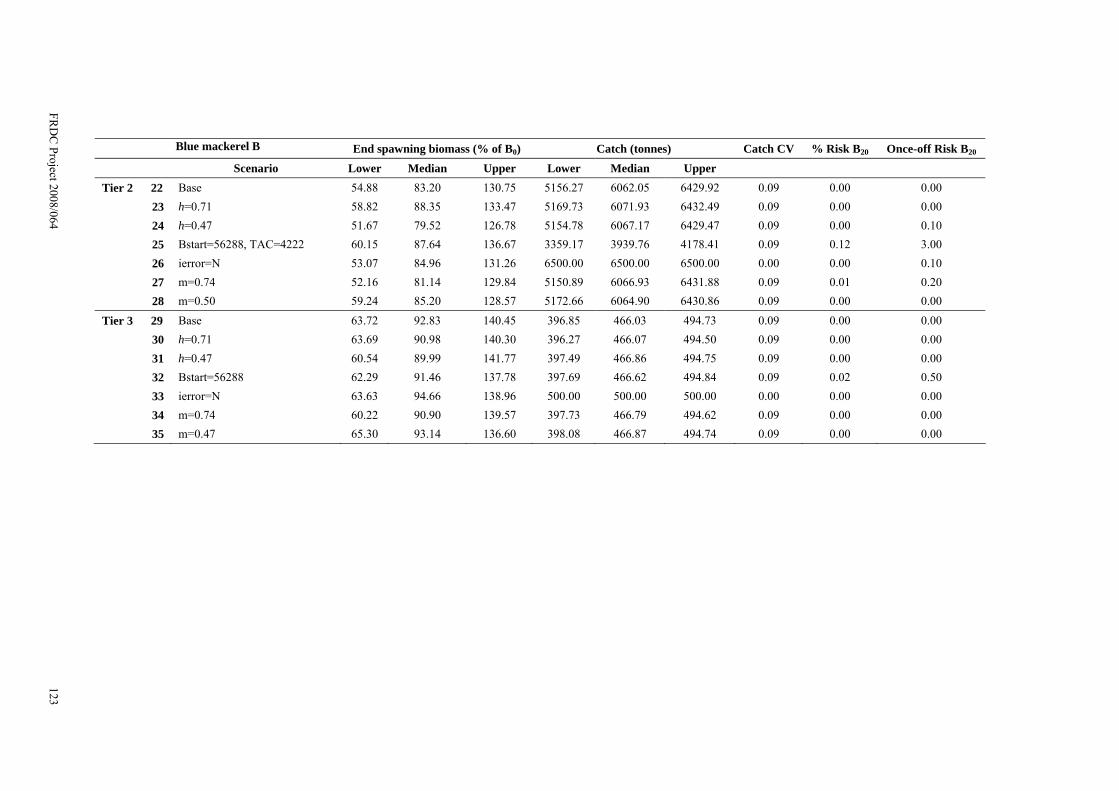
Blue mackerel B End spawning biomass (% of B0) Catch (tonnes) Catch CV % Risk B20 Once-off Risk B20
Scenario Lower Median Upper Lower Median Upper Tier 2 22 Base 54.88 83.20 130.75 5156.27 6062.05 6429.92 0.09 0.00 0.00
23 h=0.71 58.82 88.35 133.47 5169.73 6071.93 6432.49 0.09 0.00 0.00 24 h=0.47 51.67 79.52 126.78 5154.78 6067.17 6429.47 0.09 0.00 0.10 25 Bstart=56288, TAC=4222 60.15 87.64 136.67 3359.17 3939.76 4178.41 0.09 0.12 3.00 26 ierror=N 53.07 84.96 131.26 6500.00 6500.00 6500.00 0.00 0.00 0.10 27 m=0.74 52.16 81.14 129.84 5150.89 6066.93 6431.88 0.09 0.01 0.20 28 m=0.50 59.24 85.20 128.57 5172.66 6064.90 6430.86 0.09 0.00 0.00
Tier 3 29 Base 63.72 92.83 140.45 396.85 466.03 494.73 0.09 0.00 0.00 30 h=0.71 63.69 90.98 140.30 396.27 466.07 494.50 0.09 0.00 0.00 31 h=0.47 60.54 89.99 141.77 397.49 466.86 494.75 0.09 0.00 0.00 32 Bstart=56288 62.29 91.46 137.78 397.69 466.62 494.84 0.09 0.02 0.50 33 ierror=N 63.63 94.66 138.96 500.00 500.00 500.00 0.00 0.00 0.00 34 m=0.74 60.22 90.90 139.57 397.73 466.79 494.62 0.09 0.00 0.00 35 m=0.47 65.30 93.14 136.60 398.08 466.87 494.74 0.09 0.00 0.00
FRD
C Project 2008/064
123

FRD
C Project 2008/064
124

FRD
C Project 2008/064
125

FRD
C Project 2008/064
126

FRD
C Project 2008/064
127

FRD
C Project 2008/064
128

Jack mackerel Jack mackerel End spawning biomass (% of B0) Catch (tonnes) Catch CV % Risk B20 Once-off Risk B20
Scenario Lower Median Upper Lower Median Upper 1 No harvest 77.41 99.23 125.75 0.00 0.00 0.00 0.00 0.00 0.00
Tier 1 2 Base 31.77 48.39 70.28 17277.16 36743.20 72575.28 0.55 1.06 11.50 3 h=0.90 34.15 51.95 76.00 19747.39 40863.40 76228.64 0.52 0.82 9.40 4 h=0.60 27.34 43.29 64.52 14631.71 31864.52 63620.28 0.56 1.47 12.90 5 SRvari=0.3 36.16 49.56 63.06 19652.61 37902.99 70182.14 0.50 0.39 4.10 6 freq=1/2 29.20 41.25 59.96 21765.40 41144.56 77896.87 0.51 0.33 4.30 7 survari=0.6 18.16 45.26 70.11 8353.98 32970.15 89588.59 0.88 9.76 54.20 8 Srcorr=0.5 24.57 45.44 76.15 15138.37 36622.50 75217.92 0.60 3.34 24.80 9 Bstart=100% 32.53 48.87 71.03 17084.98 38538.21 76892.21 0.57 1.11 12.50
10 Bstart=70% 32.18 49.29 69.56 17427.68 34608.98 62102.91 0.50 1.02 9.80 11 Bstart=50% 31.20 47.45 71.57 16642.02 31216.51 55642.85 0.49 0.77 8.90 12 ierror=N 28.87 45.25 67.23 17742.93 38734.92 76262.94 0.56 1.66 16.60 13 Astart=equil 31.41 48.53 72.12 16560.53 34060.92 65497.87 0.53 1.06 11.00 14 m=0.31 34.57 52.89 76.21 13228.26 27153.77 51017.10 0.52 0.56 6.80 15 m=0.21 27.92 42.09 61.02 23765.65 52924.56 108430.69 0.58 1.95 16.80 16 ierror=N, bias=50% 24.60 37.15 53.21 23511.09 44297.08 85657.20 0.48 1.43 16.80 17 maxHProp=0.15, decay=0 31.89 49.03 72.27 19016.35 38290.52 70360.72 0.49 0.87 11.60 18 maxHProp=0.075, decay=0 49.70 66.57 90.79 14404.45 25302.80 41732.46 0.42 0.00 0.00
FRD
C Project 2008/064
129

Jack mackerel End spawning biomass (% of B0) Catch (tonnes) Catch CV % Risk B20 Once-off Risk B20
Scenario Lower Median Upper Lower Median Upper Tier 2 19 Base 72.54 92.79 118.08 3986.03 4662.35 4945.90 0.09 0.00 0.00
20 h=0.90 72.58 92.36 120.01 3974.48 4664.81 4947.87 0.09 0.00 0.00 21 h=0.60 69.92 90.07 116.63 3969.14 4669.05 4947.12 0.09 0.00 0.00 22 TAC=6146 71.16 92.18 119.98 4874.68 5732.56 6082.86 0.09 0.00 0.00 23 ierror=N 71.56 92.56 119.85 5000.00 5000.00 5000.00 0.00 0.00 0.00 24 m=0.31 69.87 90.31 117.85 3981.95 4665.53 4948.93 0.09 0.00 0.00 25 m=0.21 75.80 94.41 120.15 3970.44 4669.20 4947.93 0.09 0.00 0.00
Tier 3 26 Base 76.17 95.50 124.48 397.42 467.20 495.03 0.09 0.00 0.00 27 h=0.90 75.50 96.76 124.18 397.06 466.05 494.69 0.09 0.00 0.00 28 h=0.60 77.52 97.25 126.54 396.94 466.67 494.68 0.09 0.00 0.00 29 ierror=N 76.50 97.15 122.31 500.00 500.00 500.00 0.00 0.00 0.00 30 m=0.31 74.38 96.60 124.85 397.77 466.64 494.88 0.09 0.00 0.00 31 m=0.21 78.54 97.08 121.87 396.64 466.54 494.69 0.09 0.00 0.00
FRD
C Project 2008/064
130

FRD
C Project 2008/064
131

FRD
C Project 2008/064
132

FRD
C Project 2008/064
133

FRD
C Project 2008/064
134

Australian sardine (east) Australian sardine End spawning biomass (% of B0) Catch (tonnes) Catch CV % Risk B20 Once-off Risk B20
Scenario Lower Median Upper Lower Median Upper 1 No harvest 65.91 92.62 133.92 0.00 0.00 0.00 0.00 0.00 0.00
Tier 1 2 Base 38.05 65.30 102.57 1362.36 2770.22 5167.73 0.52 0.30 4.70 3 h=0.71 42.69 66.59 103.78 1546.97 3098.01 5795.05 0.52 0.19 3.70 4 h=0.47 34.66 57.83 93.33 1056.17 2239.00 4289.50 0.55 0.60 7.40 5 SRvari=0.3 52.81 68.97 87.71 1595.22 2864.22 4911.65 0.44 0.00 0.00 6 freq=1/2 38.16 58.03 89.09 1713.25 3190.73 5688.09 0.48 0.08 2.00 7 survari=0.6 31.64 61.43 102.20 906.59 2606.90 6349.86 0.76 2.07 26.70 8 Srcorr=0.5 28.73 56.73 114.08 1081.55 2647.37 5480.06 0.66 2.28 21.30 9 Bstart=100% 38.27 63.26 99.64 1369.99 2827.91 5398.03 0.54 0.24 4.00
10 Bstart=70% 39.91 64.33 100.98 1320.64 2593.57 4812.94 0.53 0.27 4.40 11 Bstart=50% 39.69 63.50 102.99 1247.02 2399.26 4643.72 0.55 0.21 3.90 12 Bstart=28809 37.86 64.86 101.87 1394.98 2841.22 4945.74 0.50 0.22 3.50 13 Bstart=28809, m=0.74 40.43 66.92 106.10 964.63 2122.10 4265.64 0.54 0.14 2.90 14 Bstart=28809, m=0.50 36.24 59.12 94.46 2022.58 3840.13 7002.91 0.51 0.42 6.10 15 ierror=N 36.85 62.77 102.68 1430.16 2923.44 5525.27 0.53 0.30 5.70 16 Astart=equil 37.90 63.12 99.91 1324.83 2707.91 5123.26 0.54 0.34 5.40 17 m=0.74 42.41 68.24 106.19 947.38 1912.67 3589.42 0.52 0.15 2.80 18 m=0.50 36.41 59.17 92.50 2039.65 4203.61 7890.24 0.53 0.42 5.90 19 ierror=N, bias=50% 32.48 53.71 84.89 1918.46 3655.64 6308.98 0.43 0.42 7.10 20 maxHProp=0.15, decay=0 37.88 63.34 99.90 1430.37 2823.35 5012.54 0.48 0.32 6.20 21 maxHProp=0.075, decay=0 52.53 78.12 114.48 949.67 1648.86 2839.62 0.45 0.00 0.00
FRD
C Project 2008/064
135

Australian sardine End spawning biomass (% of B0) Catch (tonnes) Catch CV % Risk B20 Once-off Risk B20
Scenario Lower Median Upper Lower Median Upper Tier 2 22 Base 35.73 63.89 104.47 2371.36 2797.31 2968.51 0.09 0.48 3.60
23 h=0.71 45.37 72.60 114.81 2392.06 2802.74 2969.38 0.09 0.04 0.70 24 h=0.47 9.15 43.60 85.11 2251.08 2780.23 2966.09 0.14 7.76 31.90 25 Bstart=28809, TAC=2161 47.36 74.61 113.80 1719.97 2017.88 2138.07 0.09 0.05 0.90 26 ierror=N 31.87 59.68 99.21 3000.00 3000.00 3000.00 0.02 1.13 9.00 27 m=0.74 24.35 51.06 89.75 2308.82 2786.88 2966.85 0.11 3.39 26.00 28 m=0.50 48.85 74.83 112.04 2371.25 2797.01 2969.00 0.09 0.01 0.20
Tier 3 29 Base 62.61 89.75 131.11 397.22 466.40 494.68 0.09 0.00 0.00 30 h=0.71 63.71 90.28 133.34 396.48 466.35 494.66 0.09 0.00 0.00 31 h=0.47 58.10 86.87 129.69 396.43 466.34 494.75 0.09 0.00 0.00 32 Bstart=28809 62.66 90.37 131.30 396.87 466.20 494.79 0.09 0.00 0.00 33 ierror=N 62.16 89.30 130.42 500.00 500.00 500.00 0.00 0.00 0.00 34 m=0.74 60.37 89.66 130.73 397.49 466.86 494.75 0.09 0.00 0.00 35 m=0.50 65.91 91.74 126.03 396.45 466.47 494.76 0.09 0.00 0.00
FRD
C Project 2008/064
136

FRD
C Project 2008/064
137

FRD
C Project 2008/064
138

FRD
C Project 2008/064
139

FRD
C Project 2008/064
140

FRD
C Project 2008/064
141

Test case: Australian sardine (west) SA Note: This test case uses weight-at-age, fecundity-at-age and selectivity-at-age from Australian sardine (east) data
Australian sardine SA End spawning biomass (% of B0) Catch (tonnes) Catch CV % Risk B20 Once-off Risk B20 Scenario Lower Median Upper Lower Median Upper
1 No harvest 65.72 93.06 137.22 0.00 0.00 0.00 0.00 0.00 0.00
Tier 1 2 Base 41.45 67.12 107.56 735.12 1455.04 2703.17 0.51 0.06 1.70 3 h=0.71 42.36 70.31 108.32 815.05 1617.23 2969.09 0.51 0.06 1.60 4 h=0.47 38.77 63.19 102.76 595.66 1200.98 2248.56 0.53 0.22 3.70 5 SRvari=0.3 56.46 73.48 91.76 858.99 1514.65 2552.00 0.43 0.00 0.00 6 freq=1/2 40.75 61.62 93.38 913.52 1688.28 3013.55 0.48 0.03 0.80 7 survari=0.6 38.70 64.61 102.06 510.81 1377.53 3303.83 0.74 0.59 11.30 8 Srcorr=0.5 31.54 61.11 114.94 603.08 1370.91 2777.57 0.62 1.20 13.00 9 Bstart=100% 42.09 65.97 107.40 750.08 1497.93 2786.30 0.51 0.08 1.90
10 Bstart=70% 42.66 66.11 107.01 697.88 1350.09 2513.18 0.53 0.14 3.10 11 Bstart=50% 41.98 66.85 103.02 629.90 1225.00 2402.39 0.56 0.13 2.60 12 Bstart=262990 42.89 68.34 107.62 714.22 1833.95 32217.78 1.62 0.24 6.00 13 Bstart=96864 41.97 68.32 107.63 772.36 1868.97 11879.16 1.16 0.10 2.30 14 Bstart=160845 43.52 67.43 105.49 748.74 1873.94 19688.38 1.42 0.10 2.20 15 h=0.71, Bstart=160845 43.19 70.39 114.41 840.76 2107.47 19694.31 1.38 0.15 3.40 16 h=0.47, Bstart=160845 39.00 62.64 100.67 617.42 1609.79 19699.97 1.48 0.22 4.80 17 Bstart=160845, m=0.74 41.89 70.36 113.59 468.71 1201.66 19699.56 1.65 0.16 3.60 18 Bstart=160845, m=0.50 39.60 63.68 101.76 1196.72 3008.44 19696.86 1.16 0.32 6.50 19 ierror=N 41.12 64.25 103.30 794.24 1567.28 2895.31 0.51 0.14 3.20 20 Astart=equil 42.86 68.65 105.83 729.37 1444.30 2661.35 0.52 0.09 1.70 21 m=0.74 41.59 69.45 112.17 466.01 921.70 1732.11 0.53 0.08 1.70 22 m=0.50 39.05 62.62 100.77 1197.41 2371.32 4403.04 0.52 0.15 3.00 23 ierror=N, bias=50% 34.39 55.57 95.41 1119.98 2053.62 3567.23 0.43 0.39 7.60 24 maxHProp=0.15, decay=0 41.99 68.77 106.33 782.40 1483.76 2583.30 0.47 0.07 2.00 25 maxHProp=0.075, decay=0 52.61 78.46 119.69 485.06 836.32 1448.97 0.45 0.00 0.00
FRD
C Project 2008/064
142

Australian sardine SA End spawning biomass (% of B0) Catch (tonnes) Catch CV % Risk B20 Once-off Risk B20
Scenario Lower Median Upper Lower Median Upper 26 Bstart=262990 39.29 62.50 100.63 1429.33 3417.61 32236.73 1.41 0.40 6.60 27 Bstart=96864 39.06 64.14 100.23 1401.93 3161.80 11879.66 0.87 0.30 4.20 28 Bstart=160845 40.23 63.76 101.20 1411.60 3265.48 19683.73 1.15 0.26 5.30 29 h=0.71, Bstart=160845 41.96 67.68 107.93 1610.79 3596.46 19750.12 1.09 0.26 5.00 30 h=0.47, Bstart=160845 34.97 57.14 93.55 1122.83 2785.67 19717.92 1.24 0.59 8.50 31 Bstart=160845, m=0.74 40.46 69.07 106.91 967.93 2144.98 19726.67 1.40 0.20 3.90 32 Bstart=160845, m=0.50 38.01 60.01 93.75 2069.43 5009.20 19854.12 0.90 0.75 9.00
FRD
C Project 2008/064
143

FRD
C Project 2008/064
144

FRD
C Project 2008/064
145

FRD
C Project 2008/064
146

FRD
C Project 2008/064
147

FRDC Project 2008/064 148
Appendix F. MSE workshop minutes Minutes
FRDC Project 2008/064: ‘Tactical Response Fund: Management Strategy Evaluation (MSE) of the harvest strategy for the Small Pelagic Fishery’
Workshop No. 1
Date: 15 December 2008 Start Time: 10:15am Location: AFMA Board Room Attendees: Gavin Begg (Chair), Emma Lawrence, Fiona Giannini, Patty Hobsbawn (BRS), Amanda Parr (AFMA), Tim Ward (SARDI), Jeremy Lyle (TAFI), Grant Pullen (TAS DPIW), Denis Brown, Gerry Geen, Terry Romaro (industry), Graham Pike (recreational), Jon Bryan (ENGO) Apologies: Selina Stoute (AFMA) 1. Welcome and introductions Gavin Begg opened the workshop and provided a brief overview of the workshop objectives and desired outcomes, which included:
• providing a description and understanding of management strategy evaluation (MSE) • identifying sources of data for use in the redeveloped Small Pelagic Fishery (SPF) MSE • seeking stakeholder input to the SPF Research Plan, designed around meeting the needs of
the SPF Harvest Strategy. 2. Overview Tim Ward gave a presentation on the SPF Harvest Strategy as a precursor to the workshop objectives. In particular it was noted that:
• the SPF has received significant government funding for its size • CPUE is not a good indicator of abundance for small pelagic species • DEPM surveys are the best way of obtaining stock size estimates for small pelagic species
and are currently used to underpin Tier 1 of the SPF Harvest Strategy • target species fall into two groups, short lived and long lived species which may need to
be factored in to the MSE • the SPF Harvest Strategy may be conservative for short lived species • the SPF Harvest Strategy has three tiers based on the level of information for determining
RBCs in the fishery. Patty Hobsbawn provided an overview of the project and reiterated the objectives and outcomes for the workshop. Key points raised were:

FRDC Project 2008/064 149
• the SPF Harvest Strategy was developed in accordance with the Commonwealth Harvest Strategy Policy (HSP)
• the HSP recommended the use of MSE to assess robustness of Commonwealth fisheries harvest strategies
• the Knuckey et al. review of the SPF Harvest Strategy included a preliminary examination of the Harvest Strategy using an MSE
• the MSE Project was developed because the MSE model code used in the Knuckey et al. review was not available to the SPFRAG/MAC on an ongoing basis
• the MSE component of the Knuckey et al. review was not a primary objective of the review and a more thorough investigation of models and data sources was deemed necessary.
A range of questions were asked as to the similarity and complexity of the proposed SPF MSE model to those used in stock assessments in other fisheries, e.g. the South East Trawl. It was noted that the two processes are similar, albeit that the MSE being developed for the SPF is a more basic model due to time, money and data constraints and importantly is not used to produce estimates of stock abundance and biomass. The key drivers of the model (e.g. age structure, DEPM biomass, recruitment) were briefly discussed. It was agreed that a more comprehensive presentation of the model would be given at the next workshop. 3. MSE and model Emma Lawrence gave a brief presentation on the principles of MSE and the benefits of using such an approach to assess the SPF Harvest Strategy. Key points discussed were:
• MSE enable the evaluation of multiple and conflicting management objectives from multiple stakeholders
• there is a high level of uncertainty about the SPF resources • MSE can be used to assess the consequences of a range of management options • MSE is not seeking an optimal strategy.
4. Data requirements for MSE of SPF Species Patty Hobsbawn went through the spreadsheet of data requirements for each of the seven stocks: eastern redbait, western redbait, eastern blue mackerel, western blue mackerel, eastern jack mackerel, western jack mackerel and eastern Australian sardine. The group identified key references and data sources for each stock that would provide inputs of real data for the model. Comment was made about the high level of uncertainty around inputs to the model, such as natural mortality rates and fishing selectivity. It was suggested that the ERAs currently being developed could be useful in determining fishing selectivity. It was also agreed that a sensitivity analysis should be conducted on each of the parameters of the model. Comment was made that when considering recruitment, fecundity at age should be considered, and that the sensitivity analyses should consider stochastic versus constant recruitment.

FRDC Project 2008/064 150
5. Research Plan Significant discussions were held about the SPF Research Plan and the different data requirements for assessment at each tier level. Basic data requirements for each tier level were identified as the following:
• Tier 3 requires catch and effort data • Tier 2 requires catch, effort and length/age data • Tier 1 requires catch, effort, length/age data and DEPM surveys.
There were concerns that the entire geographic range of stocks were not being sampled in the DEPM surveys and that this would mean the RBCs were being set lower than they otherwise would be. Items identified for the Research Plan were:
Tier Actions
1 • Annual fishery assessment report – provide an update of catch and effort data, including all jurisdictions and sectors
• Study to conduct DEPM assessment of jack mackerel from archived samples • Conduct DEPM surveys and analysis at least once every five years for each required stock • Analysis of costs for DEPM surveys for each stock • Examine options for multi-species DEPM surveys
2 • Annual fishery assessment report – provide an update of catch and effort data, including all jurisdictions and sectors
• Analysis of industry collected samples, with subsample used for ageing – include costings and program for sample collection, storage and analysis
• Analysis of fishery collected shot-by-shot data – examine variability to design monitoring program • Study to determine optimal sampling frequency for length/age data and design of appropriate
monitoring program • AFMA to provide documentation outlining justification of numbers in SPF Harvest Strategy for Tier 2
3 • Desktop review of available biological and catch data (form part of annual fishery assessment report) • Annual fishery assessment report – provide an update of catch and effort data, including all
jurisdictions and sectors
Concerns were raised that multi-species DEPM surveys may be optimal for one species and not others, but further work was required to assess the cost-effectiveness and utility of these types of surveys.

FRDC Project 2008/064 151
6. Where to from here: • develop MSE model • collate data inputs • evaluate harvest strategies • draft Research Plan • 2nd Workshop – present results • draft report for comment • final report.
7. Next workshop to present the model and MSE results for the SPF Harvest Strategy to be held
in March 2009. Meeting Ended: 4:00 pm

FRDC Project 2008/064 152
Appendix G. Case study of sample design to estimate proportion of catch-at-age for redbait The proportions of catch-at-age are important statistics for quantitative stock assessment and input data to the MSE in this report. The unit cost of estimating the age of fish means that obtaining reliable direct estimates becomes prohibitive in terms of cost. Age-length keys have been used to try to exploit the correlation between fish length and age and the fact that fish lengths can be sampled at relatively low cost. Ricker (1975, p. 205) points out that if age-length keys are to be used they should be constructed for the same stock taken during the same fishing season and with the same fishing gear as the auxiliary length data. Ewing and Lyle (2009) found evidence of a marked difference in length at sexual maturity of redbait caught in south western Tasmania between 2004 and 2006 compared with those caught in eastern Tasmania during the same period.
0 2 4 6 8 10 12
100
150
200
250
300
Age (Years)
FL (m
m)
EastSouth
0 2 4 6 8 10 12
100
150
200
250
300
Age (Years)
FL (m
m)
20032005
Figure G.1: Relationship between average fork length (FL) and age of redbait sampled in south western and eastern regions of Tasmania all years between 2003 and 2006 (left) and eastern fishery in 2003 and 2005. Bivariate age-length data collected between 2003 and 2006 suggest that young redbait caught in the south western region during this period had longer fork length, on average, than those caught in the eastern region. The data also suggest a significant change in the relationship between average fork length and age of redbait caught within regions over time, although this difference appears to be less pronounced. Differences such as these mean that estimates of proportions of redbait catch-at-age using age-length keys comprising data from catches made in different regions from different years can be biased. The requirement that age-length keys be produced from data sampled in the same years as the age proportion estimates reduces the potential of age-length keys to save sampling costs.

FRDC Project 2008/064 153
The design of a sampling scheme to estimate the proportion of fish catch-at-age using an age-length key can be approached as a two stage sampling problem, with the first stage consisting of a random sample of lengths and the second stage consisting of either a random subsample of ages or a stratified subsample of ages with intervals of length forming the strata. Lai (1993) describes a method which for a given survey budget and per-unit cost for first and second stage sampling specifies an optimal two stage sample design. Precision is optimised by minimising a quadratic loss function. For general analytical purposes, the proportion of all age classes is likely to be of similar importance (Smith 1989). In this case, the quadratic loss function reduces to the Kimura’s ‘vartot’ criterion (see for example Lai, 1993) and can be approximated by:
Nb
naL
ii
i +≅ ∑ =1Loss
where ( )ijijA
j ii qqla ˆ1ˆˆ1
2 −= ∑ =
( )2.1 1ˆˆˆ
jijL
i
A
j i pqlb −= ∑ ∑= =
in is the number of fish from the ith length strata subsampled for aging
N is the total number of length samples
NN
l ii =ˆ is the estimated proportion of fish caught in the ith length strata.
iN is the number of fish lengths measured in the ith length strata.
L is the number of length strata A is the number of age classes
i
ijij n
nq =ˆ is the estimated proportion in the ith length stratum having age class j.
The proportion of fish caught of age class j, jp.ˆ , is estimated by:
ijL
i ij qlp ˆˆˆ1. ∑ =
= (G.1)
If total survey costs are able to be approximated by the simple linear relation:
∑=+=
L
i incNc121CostTotal
where 1c is the per unit cost of collecting a random length sample and 2c is the per unit cost of aging a fish, assuming the cost of aging a fish is the same for all length classes. The optimal sampling ratio for the ith length strata is given by:
bcac
r ii
2
1* =

FRDC Project 2008/064 154
For a total survey budget, C, then, the optimal number of length samples, *N , and age subsamples, *in are given by:
∑ =+
= L
i irccCN
1*
21
* (G.2)
*** Nrn ii = (G.3)
Quinn & Deriso (1999, p.305) give an approximation for the variance of the estimates jp.ˆ as:
( ) ( ) ( )∑ = ⎥
⎥⎦
⎤
⎢⎢⎣
⎡ −+
−=
L
ijiji
i
ijijij N
pqln
qqlp
1
2.
.
ˆˆˆˆ1ˆˆˆVar
Example Redbait sampled off eastern Tasmania in the SPF in 2006 were almost exclusively between 13 cm and 23 cm. Age length data collected in 2005 and 2006 would suggest that fish of these lengths caught were between 1 and 7 years of age. It might be appropriate in this case to define
10=i length strata with each strata defined by a 1 cm length interval, between 13-14 cm and 22-23 cm, and j = 6 age classes for fish from 1-2 years, up to 6-7 years. In this case, using the data collected in 2005 and 2006, we obtain an age-length key as below:

FRDC Project 2008/064 155
Table G.2: Age-length key produced using redbait sampled in 2005 and 2006 in the eastern Tasmania region of the SPF.
Age
Length Interval il̂ 1 2 3 4 5 6
13 0.057 24 4 0 0 0 0 14 0.215 8 5 0 0 0 0 15 0.217 6 3 11 0 0 0 16 0.204 2 5 6 2 0 0 17 0.160 0 17 7 4 0 0 18 0.076 0 11 9 7 0 0 19 0.042 1 7 11 5 2 1 20 0.020 0 3 8 6 3 1 21 0.006 0 2 2 2 3 1 22 0.002 0 1 5 2 1 1
Using Equation G.1 we obtain estimated proportions of redbait catch-at-age in 2006 as
( )%3.0%,8.0,5.8%,4.29,%5.33%,6.27ˆ . ≅jp , respectively for the six age classes.
For a total survey budget of C = $5000 and assuming per unit costs of sampling a length,
1$1 =c and of obtaining an age estimate, 10$2 =c , we obtain, using Equation G.2, an optimal
first stage sample size of 690* =N length samples, and using Equation G.3, optimal second stage subsample sizes of ( )1,3,10,20,35,67,97,95,84,16* ≅in , respectively for the 10 length classes, although common sense would suggest that age estimates be obtained for all fish over 20 cm sampled in the first stage. The redbait data from 2005 and 2006 would suggest that the specified sampling design might be expected to yield variance in estimates of the order
( ) ( )44333. 105,101,1032,104,104,102ˆVar −−−−− ××××××≅jp , respectively for the six age
classes. It might be observed that the total second stage sample size, n=431, seems high relative to the optimal primary sample size of n=690. Ricker (1975, p. 207) advises that improvements in precision from using an age-length key are ‘not very great’ and that unless a large length sample is required for some other purpose, it is usually more profitable to put all resources into increasing the size of the age sample rather than collecting a large number of length samples. The very slight improvement in precision associated with the sampling lengths is unlikely to justify the additional sampling effort and additional complexity in sampling and estimation associated with a two stage sample. Accordingly, a one-stage sampling of ages (and lengths) should be the preferred option.
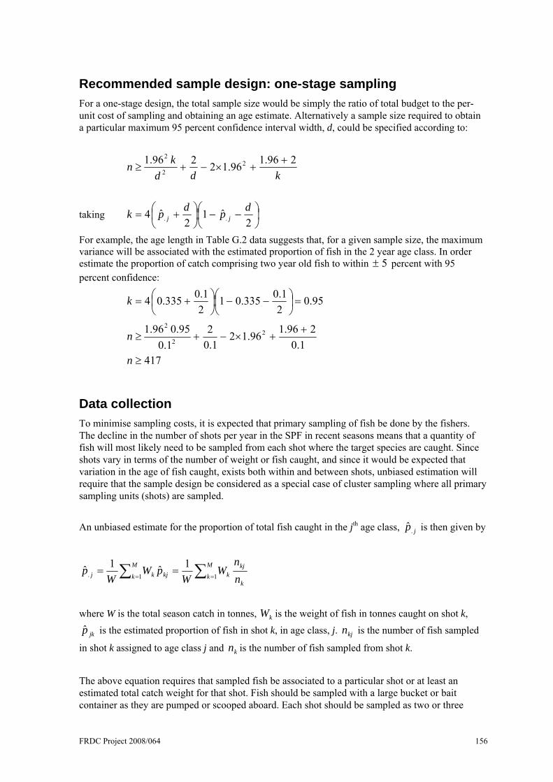
FRDC Project 2008/064 156
Recommended sample design: one-stage sampling For a one-stage design, the total sample size would be simply the ratio of total budget to the per-unit cost of sampling and obtaining an age estimate. Alternatively a sample size required to obtain a particular maximum 95 percent confidence interval width, d, could be specified according to:
kddkn 296.196.12296.1 2
2
2 ++×−+≥
taking ⎟⎠⎞
⎜⎝⎛ −−⎟⎠⎞
⎜⎝⎛ +=
2ˆ1
2ˆ4 ..
dpdpk jj
For example, the age length in Table G.2 data suggests that, for a given sample size, the maximum variance will be associated with the estimated proportion of fish in the 2 year age class. In order estimate the proportion of catch comprising two year old fish to within 5± percent with 95 percent confidence:
95.021.0335.01
21.0335.04 =⎟
⎠⎞
⎜⎝⎛ −−⎟⎠⎞
⎜⎝⎛ +=k
1.0296.196.12
1.02
1.095.096.1 2
2
2 ++×−+≥n
417≥n
Data collection To minimise sampling costs, it is expected that primary sampling of fish be done by the fishers. The decline in the number of shots per year in the SPF in recent seasons means that a quantity of fish will most likely need to be sampled from each shot where the target species are caught. Since shots vary in terms of the number of weight or fish caught, and since it would be expected that variation in the age of fish caught, exists both within and between shots, unbiased estimation will require that the sample design be considered as a special case of cluster sampling where all primary sampling units (shots) are sampled. An unbiased estimate for the proportion of total fish caught in the jth age class, jp.ˆ is then given by
k
kjM
k kkjM
k kj nn
WW
pWW
p ∑∑ ====
11.1ˆ1ˆ
where W is the total season catch in tonnes, kW is the weight of fish in tonnes caught on shot k,
jkp̂ is the estimated proportion of fish in shot k, in age class, j. kjn is the number of fish sampled
in shot k assigned to age class j and kn is the number of fish sampled from shot k.
The above equation requires that sampled fish be associated to a particular shot or at least an estimated total catch weight for that shot. Fish should be sampled with a large bucket or bait container as they are pumped or scooped aboard. Each shot should be sampled as two or three

FRDC Project 2008/064 157
subsamples during the scooping or pumping process ensuring as far as possible that each fish coming aboard at that time has an equal chance of being sampled. At the current level of fishing it is likely that 15 to 20 fish will need to be sampled each shot, depending on the total survey budget or required precision. If on any shot more fish are initially selected than required, all fish should be kept. Fish sampled from each shot should be set aside and kept separated from the rest of the catch (Kranz, 2007).