PONDICHERRY UNIVERSITY(A Central University)

DIRECTORATE OF DISTANCE EDUCATION

Management AccountingPaper Code : MBFM 3005

MBA - FINANCE

III Semester

TABLE OF CONTENTS

UNIT LESSON TITLE PAGE NO.

I

1.1 Management Accounting Basics 4

1.2 Responsibility Accounting 19

1.3 Transfer Pricing 23

II

2.1 Budgets and Budgetary Control 34

2.2 Standard Costing 58

2.3 Variance Analysis 66

III

3.1 Marginal Costing – Basic Concepts 110

3.2 Marginal Costing and CVP Analysis 127

3.3 Marginal Costing and Decision-making 148

IV

4.1 DU-Pont Analysis 164

4.2 Funds Flow Analysis 186

4.3 Cash Flow Analysis 211

4.4 Contemporary Issues in Management 226

V5.1 Social Cost Benefit Analysis 254

5.2 Reporting to Managment 258

Authors

ӵ Prof. S. Kumar

ӵ Prof. M. Zaheer Ahmed

ӵ Prof. Jonardan Koner

ӵ Prof. E. Raja Justics

Edited by

Prof. Malabika Deo, Professor,Dept.of Commerce, Pondicherry University,Puducherry.

© All Rights ReservedFor Private Circulation Only

TABLE OF CONTENTS

UNIT LESSON TITLE PAGE NO.

I

1.1 Management Accounting Basics 4

1.2 Responsibility Accounting 19

1.3 Transfer Pricing 23

II

2.1 Budgets and Budgetary Control 34

2.2 Standard Costing 58

2.3 Variance Analysis 66

III

3.1 Marginal Costing – Basic Concepts 110

3.2 Marginal Costing and CVP Analysis 127

3.3 Marginal Costing and Decision-making 148

IV

4.1 DU-Pont Analysis 164

4.2 Funds Flow Analysis 186

4.3 Cash Flow Analysis 211

4.4 Contemporary Issues in Management 226

V5.1 Social Cost Benefit Analysis 254

5.2 Reporting to Managment 258

Notes

1

MBA (Finance) – III Semester Paper code: MBFM3005

PAPER -XV

Management Accounting

Objectives

➢ To apply various management accounting techniques to all types of organizations for planning, decision making and control purposes in practical situations and

➢ To familiarize Contemporary Issues in Management Accounting.

Unit - I

Management accounting – Objectives, nature, and scope of Financial Accounting, Cost Accounting, and Management Accounting – Managerial Decisions – Accounting Plan and Responsibility Centers – Significance of Responsibility Accounting – Responsibility Centers – Cost Centre, Profit Centre and Investment Centre – Determinants of Responsibility Centers – Transfer Pricing – Objectives of transfer pricing – Methods of transfer pricing (simple problems) – Conflict between a division and a company - Multi-National Transfer pricing.

Unit – II

Budgeting and Budgetary control – Fixed and flexible budget – Preparation of functional budget for operating and non-operating functions, Cash budgets, Capital expenditure budget, Master budget, Principal budget factors – Zero-base budgeting – Performance budgeting – Standard Costing and Variance Analysis – Material Variances – labour Variances, Overhead (Fixed and Variable) Variances – Sales Variances.

Notes

2

Unit – III

Marginal Costing and Break-even Analysis – Cost-Volume-Profit (CVP) Analysis – Break-Even Analysis – Assumptions and practical applications of Breakeven-Analysis – Decisions regarding Sales-mix – Make or Buy Decisions – Limiting Factor Decision – Export Decision – Plant Merger – Decision of Shutdown or Continuation of a product line.

Unit - IV

DuPont Analysis – Fund Flow Analysis – Cash flow analysis – Contemporary Issues in Management Accounting – Value chain analysis – Activity-Based Costing (ABC) – Quality Costing – Target and Life Cycle Costing – Theory of Constraints accounting (TOC).

Unit – V

Social Cost Benefit Analysis – Decision Tree in Management – Reporting to Management – Objectives of Reporting – Reporting needs at different managerial levels – Types of reports – Modes of Reporting, Reporting at different levels of Management.

[Note: Distribution of Questions between Problems and Theory of this paper must be 60:40 i.e., Problem Questions: 60 % & Theory Questions: 40%]

References

Dr Murthy, S Gurusamy, MANAGEMENT ACCOUNTING, McGraw Hill, Delhi, 2009

Khan. MY, Jain P., MANAGEMENT ACCOUNTING, McGraw Hill, Delhi, 2009

Singhvi. NM, MANAGEMENT ACCOUNTING, PHI, Delhi, 2010

Notes

3

UNIT – I

Learning Objectives

After studying this unit you will be able to

➢ Understand the management accounting as an area of accounting

➢ Differentiate the management accounting with the financial accounting and cost accounting.

➢ Understand the concept of Responsibility Accounting and various types of Responsibility centers and how far it fixes the responsibilities and use of the same as device for the control mechanism under Management control structure.

➢ Understand the concept of transfer pricing

➢ Know the provisions, scope, and objectives of transfer pricing

➢ Understand different methods of the determination of transfer pricing

Unit Structure

Lesson 1.1 – Management Accounting Basics

Lesson 1.2 – Responsibility Accounting

Lesson 1.3 – Transfer Pricing

Notes

4

Lesson 1.1 - Management Accounting Basics

Introduction

A business enterprise must keep a systematic record of what happens from day-to-day events so that it can know its position clearly. Most of the business enterprises are run by the corporate sector. These business houses are required by law to prepare periodical statements in proper form showing the state of financial affairs. The systematic record of the daily events of a business leading to presentation of a complete financial picture is known as accounting. Thus, Accounting is the language of business. A business enterprise speaks through accounting. It reveals the position, especially the financial position through the language called accounting.

Meaning of Accounting

Accounting is the process of recording, classifying, summarizing, analyzing and interpreting the financial transactions of the business for the benefit of management and those parties who are interested in business such as shareholders, creditors, bankers, customers, employees and government. Thus, it is concerned with financial reporting and decision making aspects of the business.

The American Institute of Certified Public Accountants Committee on Terminology proposed in 1941 that accounting may be defined as, “The art of recording, classifying and summarizing in a significant manner and in terms of money, transactions and events which are, in part at least, of a financial character and interpreting the results thereof ”.

Branches of Accounting

Accounting can be classified into three categories:

1. Financial Accounting

2. Cost Accounting, and

3. Management Accounting

Notes

5

Financial Accounting

The term ‘Accounting’ unless otherwise specifically stated always refers to ‘Financial Accounting’. Financial Accounting is commonly carried on in the general offices of a business. It is concerned with revenues, expenses, assets and liabilities of a business house. Financial Accounting has two-fold objective, viz.

1. To ascertain the result of the business, and

2. To know the financial position of the concern.

Nature and Scope of Financial Accounting

Financial accounting is a useful tool for management as well as for external users such as shareholders, potential owners, creditors, customers, employees and government as it provides information regarding the results of its operations and the financial status of the business. The following are the functional aspects of financial accounting:-

1. Dealing with Financial Transactions

Accounting as a process deals only with those transactions which are measurable in terms of money. Anything which cannot be expressed in monetary terms does not form part of financial accounting however significant it may be.

2. Recording of information

Accounting is an art of recording financial transactions of a business concern. As there is a limitation for human memory, it is not possible to remember all transactions of the business. Therefore, the information is recorded in a set of books called Journal and other subsidiary books and it is useful for management in its decision making process.

3. Classification of Data

The recorded data are arranged in a manner so as to group the transactions of similar nature at one place so that full information of these items may be collected under different heads. This is done in the

Notes

6

book called ‘Ledger’. For example, we may have accounts called ‘Salaries’, ‘Rent’, ‘Interest’, Advertisement’, etc. To verify the arithmetical accuracy of such accounts, trial balance is prepared.

4. Summarizing Group of Information

The classified information of the trial balance is used to prepare profit and loss account and balance sheet in a manner useful to the users of accounting information. The final accounts are prepared to find out operational efficiency and financial strength of the business.

5. Analyzing

It is the process of establishing the relationship between the items of the profit and loss account and the balance sheet. The purpose is to identify the financial strength and weakness of the business. It also provides a basis for interpretation.

6. Interpreting the Financial Information

It is concerned with explaining the meaning and significance of the relationship established by the analysis. It is useful to the users, as it enables them to take correct decisions.

7. Communicating the Results

The profitability and financial position of the business as interpreted above are communicated to the interested parties at regular intervals so as to assist them to make their own conclusions.

Limitations of Financial Accounting

Financial accounting is concerned with the preparation of final accounts. The present day business has become so complex that mere final accounts are not sufficient in meeting financial needs. Financial accounting is like a post-mortem report. At the most it can reveal what has happened so far, but it does not have any control over the past happenings. The limitations of financial accounting are as follows:-

Notes

7

1. It records only quantitative information.

2. It records only the historical cost. The impact of future uncertainties has no place in financial accounting.

3. It does not take into account price level changes.

4. It provides information about the whole concern. Product-wise, process-wise, department-wise or information of any other line of activity cannot be obtained separately from the financial accounting.

5. Cost figures are not known in advance. Therefore, it is not possible to fix the price in advance. It does not provide information to increase or reduce the selling price.

6. As there is no technique for comparing the actual performance with that of the budgeted targets, it is not possible to evaluate performance of the business.

7. It does not tell about the optimum or otherwise of the quantum of profit made and does not provide the ways and means to increase the profits.

8. In case of loss, whether loss can be reduced or converted into profit by means of cost control and cost reduction? Financial accounting does not answer such question.

9. It does not reveal which departments are performing well? Which ones are incurring losses and how much is the loss in each case?

10. It does not provide the cost of products manufactured

11. There is no means provided by financial accounting to reduce the wastage.

12. Can the expenses be reduced which results in the reduction of product cost and if so, to what extent and how? There is no answer to these questions in financial accounting.

13. It is not helpful to the management in taking strategic decisions like replacement of assets, introduction of new products, discontinuation of an existing line, expansion of capacity, etc.

14. It provides ample scope for manipulation like overvaluation or undervaluation. This possibility of manipulation reduces the reliability.

15. It is technical in nature. A person not conversant with accounting has little utility of the financial accounts.

Notes

8

Cost Accounting

An accounting system is to make available necessary and accurate information for all those who are interested in the welfare of the organization. The requirements of majority of them are satisfied by means of financial accounting.

However, the management requires far more detailed information than what the conventional financial accounting can offer. The focus of the management lies not in the past but on the future.

For a businessman who manufactures goods or renders services, cost accounting is a useful tool. It was developed on account of limitations of financial accounting and is the extension of financial accounting. The advent of factory system gave an impetus to the development of cost accounting.

It is a method of accounting for cost. The process of recording and accounting for all the elements of cost is called cost accounting.

The Institute of Cost and Works Accountants, London defines costing as, “the process of accounting for cost from the point at which expenditure is incurred or committed to the establishment of its ultimate relationship with cost centres and cost units. In its wider usage it embraces the preparation of statistical data, the application of cost control methods and the ascertainment of the profitability of activities carried out or planned”.

The Institute of Cost and Works Accountants, India defines cost accounting as, “the technique and process of ascertainment of costs. Cost accounting is the process of accounting for costs, which begins with recording of expenses or the bases on which they are calculated and ends with preparation of statistical data”.

To put it simply, when the accounting process is applied for the elements of costs (i.e., Materials, Labour and Other expenses), it becomes Cost Accounting.

Notes

9

Objectives of Cost Accounting

Cost accounting was born to fulfill the needs of manufacturing companies. It is a mechanism of accounting through which costs of goods or services are ascertained and controlled for different purposes. It helps to ascertain the true cost of every operation, through a close watch, say, cost analysis and allocation.

The main objectives of cost accounting are as follows:-

1. Cost Ascertainment

2. Cost Control

3. Cost Reduction

4. Fixation of Selling Price

5. Providing information for framing business policy.

1. Cost Ascertainment

The main objective of cost accounting is to find out the cost of product, process, job, contract, service or any unit of production. It is done through various methods and techniques.

2. Cost Control

The very basic function of cost accounting is to control costs. Comparison of actual cost with standards reveals the discrepancies (Variances). The variances indicate whether cost is within control or not. Remedial actions are suggested to control the costs which are within control.

3. Cost Reduction

Cost reduction refers to the real and permanent reduction in the unit cost of goods manufactured or services rendered without affecting the use intended. It can be done with the help of techniques called budgetary control, standard costing, material control, labour control and overheads control.

Notes

10

4. Fixation of Selling Price

The price of any product consists of total cost and the margin required. Cost data are useful in the determination of selling price or quotations. It provides detailed information regarding various components of cost. It also provides information in terms of fixed cost and variable costs, so that the extent of price reduction can be decided.

5. Framing Business Policy

Cost accounting helps management in formulating business policy and decision making. Break even analysis, cost volume profit relationships, differential costing, etc are helpful in taking decisions regarding key areas of the business like-

a. Continuation or discontinuation of production

b. Utilization of capacity

c. The most profitable sales mix

d. Key factor

e. Export decision

f. Make or buy

g. Activity planning, etc.

Nature and Scope of Cost Accounting

Cost accounting is concerned with ascertainment and control of costs. The information provided by cost accounting to the management is helpful for cost control and cost reduction through functions of planning, decision making and control. Initially, cost accounting confined itself to cost ascertainment and presentation of the same, mainly to find out product cost. With the introduction of large scale production, the scope of cost accounting got widened and providing information for cost control and cost reduction assumed equal significance along with finding out cost of production. To start with cost accounting was applied in manufacturing activities but now it is applied also in service organizations, government organizations, local authorities, agricultural farms, extractive industries and so on.

Notes

11

Cost accounting guides for ascertainment of cost of production. Cost accounting discloses profitable and unprofitable activities. It helps management to eliminate the unprofitable activities. It provides information for estimate and tenders. It discloses the losses occurring in the form of idle time spoilage or scrap etc. It also provides a perpetual inventory system. It helps to make effective control over inventory and for preparation of interim financial statements. It helps in controlling the cost of production with the help of budgetary control and standard costing. Cost accounting provides data for future production policies. It discloses the relative efficiencies of different workers and for fixation of wages to workers.

Limitations of Cost Accounting

i) It is based on estimation: as cost accounting relies heavily on predetermined data, it is not reliable.

ii) No uniform procedure in cost accounting: as there is no uniform procedure, with the same information different results may be arrived by different cost accountants.

iii) Large number of conventions and estimates: There are number of conventions and estimates in preparing cost records such as materials are issued on an average (or) standard price, overheads are charged on percentage basis, Therefore, the profits arrived from the cost records are not true.

iv) Formalities are more: Many formalities are to be observed to obtain the benefit of cost accounting. Therefore, it is not applicable to small and medium firms.

v) Expensive: Cost accounting is expensive and requires reconciliation with financial records.

vi) It is unnecessary: Cost accounting is an additional tool not essential tool and an enterprise can survive even without cost accounting.

vii) Secondary data: Cost accounting depends on financial statements for a lot of information. The errors or short comings in that information creep into cost accounts also.

Notes

12

Management Accounting

Management accounting is not a specific system of accounting. It could be any form of accounting which enables a business to be conducted more effectively and efficiently. It is largely concerned with providing economic information to mangers for achieving organizational goals. It is an extension of the horizon of cost accounting towards newer areas of management.

Though much of the management accounting information are financial in nature but are organized in a manner relating directly to the decision on hand.

Management Accounting is comprised of two words ‘Management’ and ‘Accounting’. It means the study of managerial aspect of accounting. The emphasis of management accounting is to redesign accounting in such a way that it is helpful to the management in formation of policy, control of execution and appreciation of effectiveness.

Management accounting is of recent origin. This was first used in 1950 by a team of accountants visiting U. S. A under the auspices of Anglo-American Council on Productivity

Definition

Anglo-American Council on Productivity defines Management Accounting as, “the presentation of accounting information in such a way as to assist management to the creation of policy and the day to day operation of an undertaking”

The American Accounting Association defines Management Accounting as “the methods and concepts necessary for effective planning for choosing among alternative business actions and for control through the evaluation and interpretation of performances”.

The Institute of Chartered Accountants of India defines Management Accounting as follows: “Such of its techniques and procedures by which accounting mainly seeks to aid the management collectively has come to be known as management accounting”

Notes

13

From these definitions, it is very clear that financial data are recorded, analyzed and presented to the management in such a way that it becomes useful and helpful in planning and running business operations more systematically.

Objectives of Management Accounting

The fundamental objective of management accounting is to enable the management to maximize profits or minimize losses. The evolution of management accounting has given a new approach to the function of accounting. The main objectives of management accounting are as follows:

1. Planning and Policy Formulation

Planning involves forecasting on the basis of available information, setting goals; framing polices determining the alternative courses of action and deciding on the programme of activities. Management accounting can help greatly in this direction. It facilitates the preparation of statements in the light of past results and gives estimation for the future.

2. Interpretation process

Management accounting is to present financial information to the management. Financial information is technical in nature.

Therefore, it must be presented in such a way that it is easily understood. It presents accounting information with the help of statistical devices like charts, diagrams, graphs, etc.

3. Assists in Decision-Making Process

With the help of various modern techniques management accounting makes decision-making process more scientific. Data relating to cost, price, profit and savings for each of the available alternatives are collected and analyzed and thus it provides a base for taking sound decisions.

Notes

14

4. Controlling

Management accounting is a useful tool for managerial control. Management accounting tools like standard costing and budgetary control are helpful in controlling performance.

Cost control is affected through the use of standard costing and departmental control is made possible through the use of budgets. Performance of each and every individual operation is controlled with the help of management accounting.

5. Reporting

Management accounting keeps the management fully informed about the latest position of the concern through reporting. It helps management to take proper and quick decisions. The performances of various departments are regularly reported to the top management.

6. Facilitates Organizing

Since management accounting stresses more on Responsibility Centers with a view to control costs and responsibilities, it also facilitates decentralization to a greater extent.

Thus, it is helpful in setting up effective and efficient organization framework.

7. Facilitates Coordination of Operations

Management accounting provides tools for overall control and coordination of business operations. Budgets are important means of coordination.

Nature and Scope of Management Accounting

Management accounting involves furnishing of accounting data to the management for basing its decisions. It helps in improving efficiency and achieving the organizational goals. The following paragraphs discuss about the nature of management accounting.

Notes

15

1. Provides accounting information

Management accounting is based on accounting information. Management accounting is a service function and it provides necessary information to different levels of management.

Management accounting involves the presentation of information in a way it suits managerial needs. The accounting data collected by accounting department is used for reviewing various policy decisions.

2. Cause and Effect Analysis

The role of financial accounting is limited to find out the ultimate result, i.e., profit and loss, where as management accounting goes a step further. Management accounting discusses the cause and effect relationship. The reasons for the loss are probed and the factors directly influencing the profitability are also analyzed. Profits are compared to sales, different expenditures, current assets, interest payables, share capital, etc. to give meaningful interpretation.

3. Use of Special Techniques and Concepts

Management accounting uses special techniques and concepts according to necessity, to make accounting data more useful. The techniques usually used include financial planning and analyses, standard costing, budgetary control, marginal costing, project appraisal etc.

4. Taking Important Decisions

It supplies necessary information to the management which may be useful for its decisions. The historical data is studied to see its possible impact on future decisions. The implications of various decisions are also taken into account.

5. Achieving of Objectives

Management accounting uses the accounting information in such a way that it helps in formatting plans and setting up objectives. Comparing actual performance with targeted figures will give an idea to the management about the performance of various departments. When

Notes

16

there are deviations, corrective measures can be taken at once with the help of budgetary control and standard costing.

6. No Fixed Norms

No specific rules are followed in management accounting as that of financial accounting. Though the tools are the same, their use differs from concern to concern. The deriving of conclusions also depends upon the intelligence of the management accountant. The presentation will be in the way which suits the concern most. 7. Increase in Efficiency

The purpose of using accounting information is to increase efficiency of the concern. The performance appraisal will enable the management to pin-point efficient and inefficient spots.

Effort is made to take corrective measures so that efficiency is improved. The constant review will make the staff cost – conscious.

8. Supplies Information and not Decision

Management accountant is only to guide to take decisions. The data is to be used by the management for taking various decisions. ‘How is the data to be utilized’ will depend upon the caliber and efficiency of the management.

9. Concerned with Forecasting

The management accounting is concerned with the future. It helps the management in planning and forecasting. The historical information is used to plan future course of action. The information is supplied with the object to guide management for taking future decisions.

Limitations of Management Accounting

Management Accounting is in the process of development. Hence, it suffers from all the limitations of a new discipline. Some of these limitations are:

Notes

17

1. Limitations of Accounting Records

Management accounting derives its information from financial accounting, cost accounting and other records. It is concerned with the rearrangement or modification of data.

The correctness or otherwise of the management accounting depends upon the correctness of these basic records. The limitations of these records are also the limitations of management accounting.

2. It is only a Tool

Management accounting is not an alternate or substitute for management. It is a mere tool for management. Ultimate decisions are being taken by management and not by management accounting.

3. Heavy Cost of Installation

The installation of management accounting system needs a very elaborate organization. This results in heavy investment which can be afforded only by big concerns.

4. Personal Bias

The interpretation of financial information depends upon the capacity of interpreter as one has to make a personal judgment. Personal prejudices and bias affect the objectivity of decisions.

5. Psychological Resistance

The installation of management accounting involves basic change in organization set up. New rules and regulations are also required to be framed which affect a number of personnel and hence there is a possibility of resistance form some or the other.

6. Evolutionary Stage

Management accounting is only in a developmental stage. Its concepts and conventions are not as exact and established as that of other branches of accounting.

Notes

18

Therefore, its results depend to a very great extent upon the intelligent interpretation of the data of managerial use.

7. Provides only Data

Management accounting provides data and not decisions. It only informs, not prescribes. This limitation should also be kept in mind while using the techniques of management accounting.8. Broad-based Scope

The scope of management accounting is wide and this creates many difficulties in the implementations process. Management requires information from both accounting as well as non-accounting sources. It leads to inexactness and subjectivity in the conclusion obtained through it.

****

Notes

19

Lesson 1.2 - Responsibility Accounting

Definition of Responsibility Accounting

“Responsibility Accounting collects and reports planned and actual accounting information about the inputs and outputs of responsibility centers”.

It is based on information pertaining to inputs and outputs. The resources utilized in an organization are physical in nature like quantities of materials consumed, hours of labour, etc., which are called inputs. They are converted into a common denominator and expressed in monetary terms called “costs”, for the purpose of managerial control. In a similar way, outputs are based on cost and revenue data.

Responsibility Accounting must be designed to suit the existing structure of the organization. Responsibility should be coupled with authority. An organization structure with clear assignment of authorities and responsibilities should exist for the successful functioning of the responsibility accounting system. The performance of each manager is evaluated in terms of such factors.

Responsibility Centres

The main focus of responsibility accounting lies on the responsibility centres. A responsibility centre is a sub unit of an organization under the control of a manager who is held responsible for the activities of that centre. The responsibility centres are classified as follows:-

1) Cost Centres,

2) Profit Centres and

3) Investment centres.

Notes

20

Cost Centres

When the manager is held accountable only for costs incurred in a responsibility centre, it is called a cost centre. It is the inputs and not outputs that are measured in terms of money. A cost centre records only costs incurred by the centre/unit/division, but the revenues earned (output) are excluded from its purview. It means that a cost centre is a segment whose performance is measured in terms of cost without taking into consideration its attainments in terms of “output”. The costs are the data for planning and control of cost canters. The performance of the managers is evaluated by comparing the costs incurred with the budgeted costs. The management focuses on the cost variances for ensuring proper control.

A cost centre does not serve the purpose of measuring the performance of the responsibility centre, since it ignores the output (revenues) measured in terms of money. For example, common feature of production department is that there are usually multiple product units. There must be some common basis to aggregate the dissimilar products to arrive at the overall output of the responsibility centre. If this is not done, the efficiency and effectiveness of the responsibility centre cannot be measure.

Profit Centres

When the manager is held responsible for both Costs (inputs) and Revenues (output) it is called a profit centre. In a profit centre, both inputs and outputs are measured in terms of money. The difference between revenues and costs represents profit. The term “revenue” is used in a different sense altogether.

According to generally accepted principles of accounting, revenues are recognized only when sales are made to external customers. For evaluating the performance of a profit centre, the revenue represents a monetary measure of output arising from a profit centre during a given period, irrespective of whether the revenue is realized or not.

The relevant profit to facilitate the evaluation of performance of a profit centre is the pre–tax profit. The profit of all the departments

Notes

21

so calculated will not necessarily be equivalent to the profit of the entire organization. The variance will arise because costs which are not attributable to any single department are excluded from the computation of the department’s profits and the same are adjusted while determining the profits of the whole organization.

Profit provides more effective appraisal of the manager’s performance. The manager of the profit centre is highly motivated in his decision-making relating to inputs and outputs so that profits can be maximized. The profit centre approach cannot be uniformly applied to all responsibility centres. The following are the criteria to be considered for making a responsibility centre into a profit centre.

A profit centre must maintain additional record keeping to measure inputs and outputs in monetary terms. When a responsibility centre renders only services to other departments, e.g., internal audit, it cannot be made a profit centre.

A profit centre will gain more meaning and significance only when the divisional managers of responsibility centers have empowered adequately in their decision making relating to quality and quantity of outputs and also their relation to costs.

If the output of a division is fairly homogeneous (e.g., cement), a profit centre will not prove to be more beneficial than a cost centre.

Due to intense competition prevailing among different profit centers, there will be continuous friction among the centers arresting the growth and expansion of the whole organization. A profit centre will generate too much of interest in the short-run profit which may be detrimental to the long-term results.

Investment Centers

When the manager is held responsible for costs and revenues as well as for the investment in assets, it is called an Investment Centre. In an investment centre, the performance is measured not by profits alone, but is involved with investments effected. The manager of an investment centre is always interested to earn a satisfactory return. The return on investment

Notes

22

is usually referred to as ROI that serves as a criterion for the performance evaluation of the manager of an investment centre. Investment centers may be considered as separate entities where the manager is entrusted with the overall responsibility of inputs, outputs and investment.

****

Notes

23

Lesson 1.3 - Transfer Pricing

Introduction

In the post economic liberalization, multinational companies started expanding their business transactions across the border. The rapid growth of economic activities of multinational groups led to various complex issues regarding taxation. The multinational groups have more inter business activities like transfer of goods or services. One group transfers the goods and services to another group. Such transfers cause the problem of pricing the goods or services.

Thus it may not comply with necessary rules and regulations while transferring goods or services. This noncompliance with statutory provisions may tend to create revenue loss to the exchequer. Hence, there is a need to provide statutory framework which will lead to compute the profits and tax in a fair manner.

Provisions Regulating Transfer Pricing in India

The Finance Act, 2001 introduced law of transfer pricing in India through sections 92A to 92F of the Indian Income Tax Act, 1961 which guides computation of the transfer price and suggests detailed documentation procedures.

Scope & Applicability

Transfer Pricing Regulations (“TPR”) are applicable to the all enterprises that enter into an ‘International Transaction’ with an ‘Associated Enterprise’. Therefore, generally it applies to all cross border transactions entered into between associated enterprises. It even applies to transactions involving a mere book entry having no apparent financial impact. The aim is to arrive at the comparable price as available to any unrelated party in open market conditions and is known as the Arm’s Length Price (‘ALP’).

Notes

24

Important Definitions

Transfer Pricing

“Transfer price” is a price at which the value of goods or services being transferred between independently operating units of an organization. But, the expression “transfer pricing” generally refers to prices of transactions between associated enterprises may be different from the prices at which an independent enterprise transfers to another the same goods or services.

Arm’s Length Price

The term arm’s length price refers to a price which is applied or proposed to be applied in a transaction between persons other than associated enterprises, in uncontrolled conditions.

Objectives of Transfer Pricing

There are three objectives that should be considered for setting-out a transfer price.

(a) Autonomy of the Division. The prices should seek to maintain the maximum divisional autonomy so that the benefits, of decentralization (motivation, better decision making, initiative etc.) are maintained. The profits of one division should not be dependent on the actions of other divisions,

(b) Goal congruence: The prices should be set so that the divisional management’s desire to maximize divisional earrings is consistent with the objectives of the company as a whole. The transfer prices should not encourage suboptimal decision-making.

(c) Performance appraisal: The prices should enable reliable assessments to be made of divisional performance.

Determination of Arm’s Length Price

The arm’s length price in relation to an international transaction can be determined by any of the following methods, The most appropriate

Notes

25

method, may be chosen having regard to the nature of transaction or class of transaction or class of associated persons or functions performed by such persons or such other relevant factors as the Board may prescribed namely:—

(a) Comparable uncontrolled price method;

(b) Resale price method;

(c) Cost plus method;

(d) Profit split method;

(e) Transactional net margin method;

Suppose more than one price is determined by the most appropriate method, the arm’s length price shall be taken to be the arithmetical mean of such prices:

In case, the variation between the arm’s length price so determined and price at which the international transaction has actually been undertaken does not exceed five per cent of the latter, the price at which the international transaction has actually been undertaken shall be deemed to be the arm’s length price.

Computation of Arm’s Length Price

The Institute of Chartered Accountant of India (ICAI) has laid down certain guidelines which are to be followed when comparable uncontrollable price is determined. The guidelines are given below.

(a) Comparable Uncontrollable Price Method

i) Find out the price charged or paid for property transferred or services provided in a comparable uncontrolled transaction, or a number of such transactions, is identified,

ii) Adjust such price to account for differences, if any, between the international transaction and the comparable uncontrolled transaction, or between the enterprises entering into such transactions, which could materially affect the price in the open market;

Notes

26

iii) the adjusted price arrived at is taken to be an arm’s length price in respect of the property transferred or services provided in the international transaction;

iv) If there is any variation between price charged (price paid) on the international transaction and arm’s length price, then an adjustment has to be made in order to remove the variance.

(b) Resale Price Method

(i) Find out the international transaction through which property purchased or services obtained

(ii) Identify the price at which the property or services are resold or provided to a third party

(iii) Deduct the normal gross profit earned by the enterprise from the resale price of such property or services. The normal gross profit can be taken of a profit on a similar transaction made with unrelated party.

iv) The price so arrived at is further reduced by the expenses incurred by the enterprise in connection with the purchase of property or obtaining of service; The price so arrived at is adjusted to take into account the functional and other differences, including differences in accounting practices, if any, between the international transaction and the comparable uncontrolled transactions, or between the enterprises entering into such transactions, which could materially affect the amount of gross profit margin in the open market;

v) the adjusted price arrived at is taken to be an arm’s length price in respect of the purchase of the property or obtaining of the services by the enterprise from the associated enterprise;

(c) Cost Plus Method

i) Find the direct and indirect costs of production incurred by the enterprise in respect of property transferred or services provided to an associated enterprise

ii) Find a comparable uncontrollable transaction or a series of transaction with a third party for same property or service

Notes

27

iii) The amount of a normal gross profit mark-up to such costs (computed according to the same accounting norms) arising from the transfer or provision of the same or similar property or services by the enterprise, or by an unrelated enterprise, in a comparable uncontrolled transaction, or a number of such transactions, is determined;

iv) The normal gross profit mark-up to account the functional and other differences, if any, between the international transaction and the comparable uncontrolled transactions,

v) The sum so arrived at, is taken to be an arm’s length price in relation to the supply of the property or provision of services by the enterprise;

d) Profit Split Method

Which may be applicable mainly in international transactions involving transfer of unique intangibles or in multiple international transactions which are so interrelated determining the arm’s length price of any one transaction, by which,

i) The combined net profit of the associated enterprises arising from the international transaction, in which they are engaged, is determined;

ii) The relative contribution made by each of the associated enterprises to the earning of such combined net profit, is then evaluated on the basis of the functions performed, assets employed or to be employed and risks assumed by each enterprise and on the basis of reliable external market data which indicates how such contribution would be evaluated by unrelated enterprise and on the basis of reliable external market data which indicates how such contribution would be evaluated by unrelated enterprises performing comparable functions in similar circumstances;

iii) The combined net profit is then split amongst the enterprises in proportion to their relative contributions,

iv) The profit thus apportioned to the assessee is taken into account to arrive at an arm’s length price in relation to the international transaction;

Notes

28

e) Transactional Net Margin Method

i) The net profit margin realized by the enterprise from an international transaction entered into with an associated enterprise is computed in relation to costs incurred or sales effected or assets employed or to be employed by the enterprise or having regard to any other relevant base;

ii) The net profit margin realised by the enterprise or by an unrelated enterprise from a comparable uncontrolled transaction or a number of such transactions is computed having regard to the same base;

iii) The net profit margin arising in comparable uncontrolled transactions is adjusted to take into account of the differences, if any, between the international transaction and the comparable uncontrolled transactions, or between the enterprises entering into such transactions, which could materially affect the amount of net profit margin in the open market;

iv) The net profit margin thus established is then taken into account to arrive at an arm’s length price in relation to be international transaction.

Illustration I

X Ltd., an Indian company, sells computer CPU to its 100 per cent subsidiary Y Ltd. in United States @ $ 50 per piece. X Ltd. also sells its computer CPU to another company Z Ltd. in United States @ $ 90 per piece. Total income of X Ltd. for the assessment year 2012-13 is 12, 00,000 which includes sales made for 100 computer CPU @ $ 50 to Y Ltd. Compute the arm’s length price and taxable income of X Ltd. The rate of one dollar may be assumed to be equivalent to 47.

Notes

29

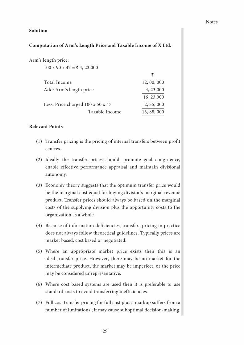
Solution

Computation of Arm’s Length Price and Taxable Income of X Ltd.

Arm’s length price: 100 x 90 x 47 = 4, 23,000 Total Income 12, 00, 000 Add: Arm’s length price 4, 23,000 16, 23,000 Less: Price charged 100 x 50 x 47 2, 35, 000 Taxable Income 13, 88, 000

Relevant Points

(1) Transfer pricing is the pricing of internal transfers between profit centres.

(2) Ideally the transfer prices should, promote goal congruence, enable effective performance appraisal and maintain divisional autonomy.

(3) Economy theory suggests that the optimum transfer price would be the marginal cost equal for buying division’s marginal revenue product. Transfer prices should always be based on the marginal costs of the supplying division plus the opportunity costs to the organization as a whole.

(4) Because of information deficiencies, transfers pricing in practice does not always follow theoretical guidelines. Typically prices are market based, cost based or negotiated.

(5) Where an appropriate market price exists then this is an ideal transfer price. However, there may be no market for the intermediate product, the market may be imperfect, or the price may be considered unrepresentative.

(6) Where cost based systems are used then it is preferable to use standard costs to avoid transferring inefficiencies.

(7) Full cost transfer pricing for full cost plus a markup suffers from a number of limitations,; it may cause suboptimal decision-making.

Notes

30

The price is only valid at one output level, it makes genuine performance appraisal difficult.

(8) Provided that variable cost equates with economic marginal cost then transfers at variable cost will avoid gross sub optimality but performance appraisal becomes meaningless.

(9) Negotiated transfer prices will only be appropriate if there is equal bargaining power and if negotiations are not protracted.

Conclusion

Transfer price policies represent the selection of suitable methods relating to the computation of transfer prices under various circumstances. More precisely, transfer pricing should be closely related to management performance assessment and decision optimization. But the problem of choosing an appropriate transfer pricing for the two functions of management-performance measurement and decision optimization –does not hold any simple solution. There is no single measure of transfer price that can be adopted under all circumstances.

Activities

1. Bring out the differences between the Financial Accounting and Cost Accounting

2. Ascertain the differences between the Financial Accounting and Management Accounting

3. Find out the differences between the Cost Accounting and Management Accounting

4. Extract the differences between the Financial Accounting and Management Accounting.

Self Assessment Questions

1. What do you understand by ‘Management Accounting’?

2. State the objectives of Management Accounting.

3. Discuss in detail the nature and scope of management accounting.

4. How can financial accounting be made useful for the management

Notes

31

accounting?

5. State the limitations of financial accounting and point out how management accounting helps in overcoming them.

6. “Accounting provides information various users”. Discuss accounting as an information system.

7. What is Responsibility Accounting? Explain the significance of Responsibility Accounting.

8. What is Transfer Pricing? Discuss the importance of Transfer Pricing.

9. What are the methods under which the arm’s length price, with regard to an international transaction is determined?

10. Write a note on the following:

i. Cost Centre

ii. Profit Centre

iii. Investment Centre

iv. Market based transfer pricing

v. Cost based transfer pricing

vi. Full cost transfer pricing

vii. Negotiated transfer pricing

viii. Variable cost transfer pricing

****

32

Notes

33

UNIT – II

Learning Objectives

After studying this unit you will be able to

➢ Understand the preparation of various operations and functional budgets of an organization

➢ Know the technique of standard costing,

➢ Differentiate between Standard Costing and Budgeting

➢ Know different types of variances

➢ Familiarize various formulas of material, labour, overheads and sales variances.

Unit Structure

Lesson 2.1 - Budgets and Budgetary Control

Lesson 2.2 - Standard Costing

Lesson 2.3 - Variance Analysis

Notes

34

Lesson 2.1 - Budgets and Budgetary Control

Introduction

To achieve the organizational objectives, an enterprise should be managed effectively and efficiently. It is facilitated by chalking out the course of action in advance. Planning, the primary function of management helps to chalk out the course of actions in advance. But planning has to be followed by continuous comparison of the actual performance with the planned performance, i. e., controlling. One systematic approach in effective follow up process is budgeting. Different budgets are prepared by the enterprise for different purposes. Thus, budgeting is an integral part of management.

Definition of Budget

‘A budget is a comprehensive and coordinated plan, expressed in financial terms, for the operations and resources of an enterprise for some specific period in the future’. (Fremgen, James M – Accounting for Managerial Analysis)

‘A budget is a predetermined detailed plan of action developed and distributed as a guide to current operations and as a partial basis for the subsequent evaluation of performance’. (Gordon and Shillinglaw)

‘A budget is a financial and/or quantitative statement, prepared prior to a defined period of time, of the policy to be pursued during the period for the purpose of attaining a given objective’. (The Chartered Institute of Management Accountants, London)

Elements of Budget

The basic elements of a budget are as follows:-

1. It is a comprehensive and coordinated plan of action.

Notes

35

2. It is a plan for the firm’s operations and resources.

3. It is based on objectives to be attained.

4. It is related to specific future period.

5. It is expressed in financial and/or physical units.

Budgeting

Budgeting is the process of preparing and using budgets to achieve management objectives. It is the systematic approach for accomplishing the planning, coordination, and control responsibilities of management by optimally utilizing the given resources.

‘The entire process of preparing the budgets is known as Budgeting’ (J. Batty)

‘Budgeting may be said to be the act of building budgets’ (Rowland & Harr)

Elements of Budgeting

1. A good budgeting should state clearly the firm’s expectations and facilitate their attainability.

2. A good budgeting system should utilize various persons at different levels while preparing the budgets.

3. The authority and responsibility should be properly fixed.

4. Realistic targets are to be fixed.

5. A good system of accounting is also essential.

6. Wholehearted support of the top management is necessary.

7. Budgeting education is to be imparted among the employees.

8. Proper reporting system should be introduced.

9. Availability of working capital is to be ensured.

Definition of Budgetary Control

CIMA, London defines budgetary control as, “the establishment of the budgets relating to the responsibility of executives to the requirements of a policy and the continuous comparison of actual with budgeted result

Notes

36

either to secure by individual action the objectives of that policy or to provide a firm basis for its revision”

‘Budgetary Control is a planning in advance of the various functions of a business so that the business as a whole is controlled’. (Wheldon)

‘Budgetary Control is a system of controlling costs which includes the preparation of budgets, coordinating the department and establishing responsibilities, comprising actual performance with the budgeted and acting upon results to achieve maximum profitability’. (Brown and Howard)

Elements of Budgetary Control

1. Establishment of budgets for each function and division of the organization.

2. Regular comparison of the actual performance with the budget to know the variations from budget and placing the responsibility of executives to achieve the desired result as estimated in the budget.

3. Taking necessary remedial action to achieve the desired objectives, if there is a variation of the actual performance from the budgeted performance.

4. Revision of budgets when the circumstances change.

5. Elimination of wastes and increasing the profitability.

Budget, Budgeting and Budgetary Control

A budget is a blue print of a plan expressed in quantitative terms. Budgeting is a technique for formulating budgets. Budgetary Control refers to the principles, procedures and practices of achieving given objectives through budgets.

According to Rowland and William, ‘Budgets are the individual objectives of a department, whereas Budgeting may be the act of building budgets. Budgetary control embraces all and in addition includes the science of planning the budgets to effect an overall management tool for the business planning and control’.

Notes

37

Objectives of Budgetary Control

Budgetary Control assists the management in the allocation of responsibilities and is a useful device to estimate and plan the future course of action. The general objectives of budgetary control are as follows:

1. Planning

(a) A budget is an action plan and it is prepared after a careful study and research.

(b) A budget operates as a mechanism through which objectives and policies are carried out.

(c) It is a communication channel among various levels of management.

(d) It is helpful in selecting a most profitable alternative.

(e) It is a complete formulation of the policy to be pursued for attaining given objectives.

2. Co-Ordination

It coordinates various activities of the business to achieve its com-mon objectives. It induces the executives to think and operate as a group.

3. Control

Control is necessary to judge that the performance of the organization confirms to the plans of business. It compares the actual performance with that of the budgeted performance, ascertains the deviations, if any, and takes corrective action at once.

Installation of Budgetary Control System

There are certain steps necessary to install a good budgetary control system in an organization. They are as follows:

1. Determination of the Objectives

2. Organization for Budgeting

3. Budget Centre

Notes

38

4. Budget Officer

5. Budget Manual

6. Budget Committee

7. Budget Period

8. Determination of Key Factor

1. Determination of Objectives

It is very clear that the installation of a budgetary control system presupposes the determination of objectives sought to be achieved by the organization in clear terms.

2. Organization for Budgeting

Having determined the objectives clearly, proper organization is essential for the successful preparation, maintenance and administration of budgets. The responsibility of each executive must be clearly defined. There should be no uncertainty regarding the jurisdiction of executives.

3. Budget Centre

It is that part of the organization for which the budget is prepared. It may be a department or any other part of the department. It is essential for the appraisal of performance of different departments so as to make them responsible for their budgets.

4. Budget Officer

A Budget Officer is a convener of the budget committee. He coordinates the budgets of various departments. The managers of different departments are made responsible for their department’s performance.

5. Budget Manual

It is a document which defines the objectives of budgetary control system. It spells out the duties and responsibilities of budget officers regarding the preparation and execution of budgets. It also specifies the relations among various functionaries.

Notes

39

6. Budget Committee

The heads of all important departments are made members of this committee. It is responsible for preparation and execution of budgets. The members of this committee may sometimes take collective decisions, if necessary. In small concerns, the accountant is made responsible for the same work.

7. Budget Period

It is the period for which a budget is prepared. It depends upon a number of factors. It may be different for different concerns/functions.

The following are the factors that may be taken into consideration while determining budget period:

a. The type of budget,

b. The nature of demand for the products,

c. The availability of finance,

d. The economic situation of the cycle and

e. The length of trade cycle

8. Determination of Key Factor

Generally, the budgets are prepared for all functional areas of the business. They are inter related and inter dependent. Therefore, a proper coordination is necessary. There may be many factors that influence the preparation of a budget.

For example, plant capacity, demand position, availability of raw materials, etc. Some factors may have an impact on other budgets also. A factor which influences all other budgets is known as Key factor.

The key factor may not remain the same. Therefore, the organization must pay due attention on the key factor in the preparation and execution of budgets.

Notes

40

Types of Budgeting

Budget can be classified into three categories from different points of view. They are:

1. According to Function

2. According to Flexibility

3. According to Time

I. According to Function

(a) Sales Budget

The budget which estimates total sales in terms of items, quantity, value, periods, areas, etc is called Sales Budget.

(b) Production Budget

It estimates quantity of production in terms of items, periods, areas, etc. It is prepared on the basis of Sales Budget.

(c) Cost of Production Budget

This budget forecasts the cost of production. Separate budgets may also be prepared for each element of costs such as direct materials budgets, direct labour budget, factory materials budgets, office overheads budget, selling and distribution overheads budget, etc.

(d) Purchase Budget

This budget forecasts the quantity and value of purchase required for production. It gives quantity wise, money wise and period wise particulars about the materials to be purchased.

(e) Personnel Budget

The budget that anticipates the quantity of personnel required during a period for production activity is known as Personnel Budget.

Notes

41

(f) Research Budget

This budget relates to the research work to be done for improvement in quality of the products or research for new products.

(g) Capital Expenditure Budget

This budget provides a guidance regarding the amount of capital that may be required for procurement of capital assets during the budget period.

(h) Cash Budget

This budget is a forecast of the cash position by time period for a specific duration of time. It states the estimated amount of cash receipts and estimation of cash payments and the likely balance of cash in hand at the end of different periods.

(i) Master Budget

It is a summary budget incorporating all functional budgets in a capsule form. It interprets different functional budgets and covers within its range the preparation of projected income statement and projected balance sheet.

II. According to Flexibility

On the basis of flexibility, budgets can be divided into two categories. They are:

1. Fixed Budget

2. Flexible Budget

1. Fixed Budget

Fixed Budget is one which is prepared on the basis of a standard or a fixed level of activity. It does not change with the change in the level of activity.

Notes

42

2. Flexible Budget

A budget prepared to give the budgeted cost of any level of activity is termed as a flexible budget. According to CIMA, London, a Flexible Budget is, ‘a budget designed to change in accordance with level of activity attained’. It is prepared by taking into account the fixed and variable elements of cost.

III. According to Time

On the basis of time, the budget can be classified as follows:

1. Long term budget

2. Short term budget

3. Current budget

4. Rolling budget

1. Long-Term Budget

A budget prepared for considerably long period of time, viz., 5 to 10 years is called Long-term Budget. It is concerned with the planning of operations of the firm. It is generally prepared in terms of physical quantities.

2. Short-Term Budget

A budget prepared generally for a period not exceeding 5 years is called Short-term Budget. It is generally prepared in terms of physical quantities and in monetary units.

3. Current Budget

It is a budget for a very short period, say, a month or a quarter. It is adjusted to current conditions. Therefore, it is called current budget.

4. Rolling Budget

It is also known as Progressive Budget. Under this method, a budget for a year in advance is prepared. A new budget is prepared after

Notes

43

the end of each month/quarter for a full year ahead. The figures for the month/quarter which has rolled down are dropped and the figures for the next month/quarter are added. This practice continues whenever a month/quarter ends and a new month/quarter begins.

Preparation of Budgets

I. Sales Budget

Sales budget is the basis for the preparation of other budgets. It is the forecast of sales to be achieved in a budget period. The sales manager is directly responsible for the preparation of this budget. The following factors are taken into consideration:

a. Past sales figures and trend

b. Salesmen’s estimates

c. Plant capacity

d. General trade position

e. Orders in hand

f. Proposed expansion

g. Seasonal fluctuations

h. Market demand

i. Availability of raw materials and other supplies

j. Financial position

k. Nature of competition

l. Cost of distribution

m. Government controls and regulations

n. Political situation.

Example

1. The Royal Industries has prepared its annual sales forecast, expecting to achieve sales of ` 30, 00,000 next year. The Controller is uncertain about the pattern of sales to be expected by month and asks you to prepare a monthly budget of sales. The following is the sales data pertained to the year, which is considered to be representative of a normal year:

Notes

44

Month Sales (`) Month Sales (`)

January 1,10,000 July 2,60,000

February 1,15,000 August 3,30,000

March 1,00,000 September 3,40,000

April 1,40,000 October 3,50,000

May 1,80,000 November 2,00,000

June 2,25,000 December 1,50,000

Prepare a monthly sales budget for the coming year on the basis of the above data.

Answer

Sales Budget

MonthSales

(given)Sales estimation based on

cash sales ratio given

January 1,10,000 (1,10,000/25,00,000) x 30,00,000 = 1,32,000

February 1,15,000 (1,15,000/25,00,000) x 30,00,000 = 1,38,000

March 1,00,000 (1,00,000/25,00,000) x 30,00,000 = 1,20,000

April 1,40,000 (1,40,000/25,00,000) x 30,00,000 = 1,68,000

May 1,80,000 (1,80,000/25,00,000) x 30,00,000 = 2,16,000

June 2,25,000 (2,25,000/25,00,000) x 30,00,000 = 2,70,000

July 2,60,000 (2,60,000/25,00,000) x 30,00,000 = 3,12,000

August 3,30,000 (3,30,000/25,00,000) x 30,00,000 = 3,96,000

September 3,40,000 (3,40,000/25,00,000) x 30,00,000 = 4,08,000

October 3,50,000 (3,50,000/25,00,000) x 30,00,000 = 4,20,000

November 2,00,000 (2,00,000/25,00,000) x 30,00,000 = 2,40,000

December 1,50,000 (1,50,000/25,00,000) x 30,00,000 = 1,80,000

Total 25,00,000 30,00,000

Note: Sales budget is prepared based on last year’s month-wise sales ratio.

Notes

45

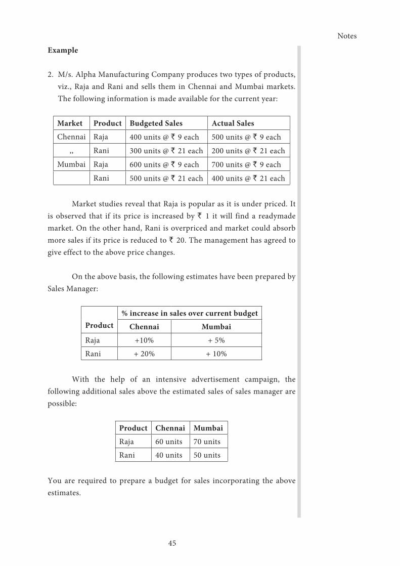
Example

2. M/s. Alpha Manufacturing Company produces two types of products, viz., Raja and Rani and sells them in Chennai and Mumbai markets. The following information is made available for the current year:

Market Product Budgeted Sales Actual Sales

Chennai Raja 400 units @ ` 9 each 500 units @ ` 9 each

,, Rani 300 units @ ` 21 each 200 units @ ` 21 each

Mumbai Raja 600 units @ ` 9 each 700 units @ ` 9 each

Rani 500 units @ ` 21 each 400 units @ ` 21 each

Market studies reveal that Raja is popular as it is under priced. It is observed that if its price is increased by ` 1 it will find a readymade market. On the other hand, Rani is overpriced and market could absorb more sales if its price is reduced to ` 20. The management has agreed to give effect to the above price changes.

On the above basis, the following estimates have been prepared by Sales Manager:

Product% increase in sales over current budget

Chennai Mumbai

Raja +10% + 5%

Rani + 20% + 10%

With the help of an intensive advertisement campaign, the following additional sales above the estimated sales of sales manager are possible:

Product Chennai Mumbai

Raja 60 units 70 units

Rani 40 units 50 units

You are required to prepare a budget for sales incorporating the above estimates.

46

AnswerSales Budget

Area ProductBudget for

current yearActual sales Budget for

future period

Units Price`

Value `

Units Price`

Value `

Units Price`

Value `

ChennaiRaja 400 9 3600 500 9 4500 500 10 5000

Rani 300 21 6300 200 21 4200 400 20 8000

Total 700 9900 700 8700 900 13000

MumbaiRaja 600 9 5400 700 9 6300 700 10 7000

Rani 500 21 10500 400 21 8400 600 20 12000

Total 1100 15900 1100 14700 1300 19000

TotalRaja 1000 9 9000 1200 9 10800 1200 10 12000

Rani 800 21 16800 600 21 12600 1000 20 20000

Total Sales

1800 25800 1800 23400 2200 32000

Workings

1. Budgeted sales for Chennai

RajaUnits

RaniUnits

Budgeted Sales 400 300

Add: Increase (10%) 40 (20%) 60

440 360

Increase due to advertisement 60 40

Total 500 400

2. Budgeted sales for Mumbai

RajaUnits

RaniUnits

Budgeted Sales 600 500

Add: Increase (5%) 30 (10%) 50

630 550

Increase due to advertisement 70 50

Total 700 600

Notes

47

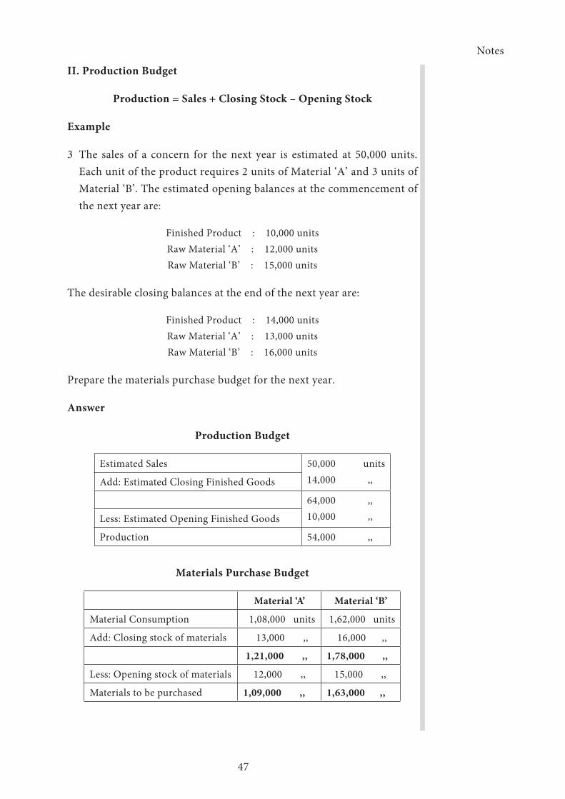
II. Production Budget

Production = Sales + Closing Stock – Opening Stock

Example

3 The sales of a concern for the next year is estimated at 50,000 units. Each unit of the product requires 2 units of Material ‘A’ and 3 units of Material ‘B’. The estimated opening balances at the commencement of the next year are:

Finished Product : 10,000 units Raw Material ‘A’ : 12,000 unitsRaw Material ‘B’ : 15,000 units

The desirable closing balances at the end of the next year are:

Finished Product : 14,000 units Raw Material ‘A’ : 13,000 unitsRaw Material ‘B’ : 16,000 units

Prepare the materials purchase budget for the next year.

Answer

Production Budget

Estimated Sales 50,000 units 14,000 ,,Add: Estimated Closing Finished Goods

64,000 ,,10,000 ,,Less: Estimated Opening Finished Goods

Production 54,000 ,,

Materials Purchase Budget

Material ‘A’ Material ‘B’

Material Consumption 1,08,000 units 1,62,000 units

Add: Closing stock of materials 13,000 ,, 16,000 ,,

1,21,000 ,, 1,78,000 ,,

Less: Opening stock of materials 12,000 ,, 15,000 ,,

Materials to be purchased 1,09,000 ,, 1,63,000 ,,

Notes

48

Workings

Materials consumption: Material ‘A’ Material ‘B’

Material required per unit of production 2 units 3 units

For production of 54,000 units 1,08,000 1,62,000

Iii. Cash Budget

It is an estimate of cash receipts and disbursements during a future period of time. “The Cash Budget is an analysis of flow of cash in a business over a future, short or long period of time. It is a forecast of expected cash intake and outlay” (Soleman, Ezra – Handbook of Business administration).

Procedure for Preparation of Cash Budget

1. First take into account the opening cash balance, if any, for the beginning of the period for which the cash budget is to be prepared.

2. Then Cash receipts from various sources are estimated. It may be from cash sales, cash collections from debtors/bills receivables, dividends, interest on investments, sale of assets, etc.

3. The Cash payments for various disbursements are also estimated. It may be for cash purchases, payment to creditors/bills payables, payment to revenue and capital expenditure, creditors for expenses, etc.

4. The estimated cash receipts are added to the opening cash balance, if any.

5. The estimated cash payments are deducted from the above proceeds.

6. The balance, if any, is the closing cash balance of the month concerned.

7. The closing cash balance is taken as the opening cash balance of the following month.

8. Then the process is repeatedly performed.

9. If the closing balance of any month is negative i.e the estimated cash payments exceed estimated cash receipts, then overdraft facility may also be arranged suitably.

Notes

49

Example

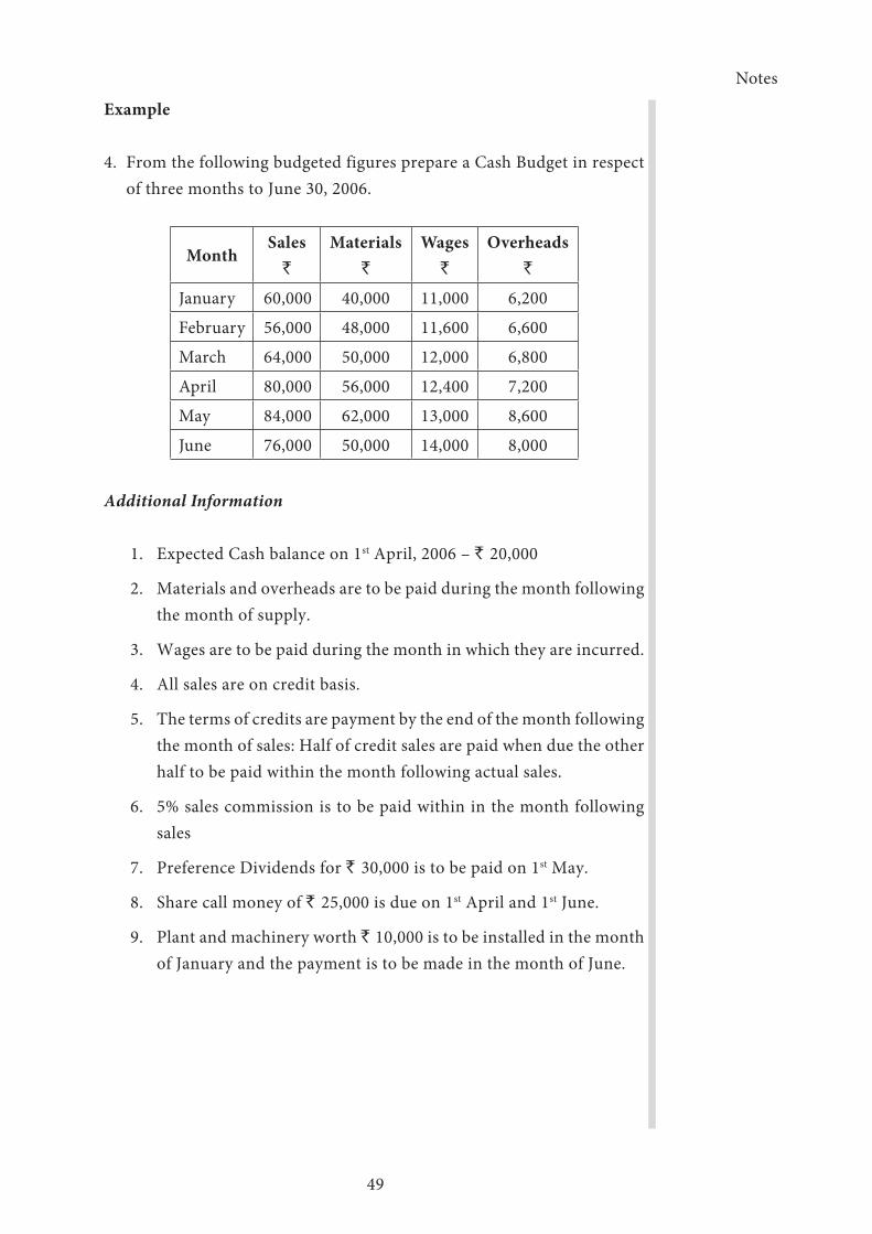
4. From the following budgeted figures prepare a Cash Budget in respect of three months to June 30, 2006.

MonthSales

`

Materials`

Wages`

Overheads`

January 60,000 40,000 11,000 6,200

February 56,000 48,000 11,600 6,600

March 64,000 50,000 12,000 6,800

April 80,000 56,000 12,400 7,200

May 84,000 62,000 13,000 8,600

June 76,000 50,000 14,000 8,000

Additional Information

1. Expected Cash balance on 1st April, 2006 – ` 20,000

2. Materials and overheads are to be paid during the month following the month of supply.

3. Wages are to be paid during the month in which they are incurred.

4. All sales are on credit basis.

5. The terms of credits are payment by the end of the month following the month of sales: Half of credit sales are paid when due the other half to be paid within the month following actual sales.

6. 5% sales commission is to be paid within in the month following sales

7. Preference Dividends for ` 30,000 is to be paid on 1st May.

8. Share call money of ` 25,000 is due on 1st April and 1st June.

9. Plant and machinery worth ` 10,000 is to be installed in the month of January and the payment is to be made in the month of June.

Notes

50

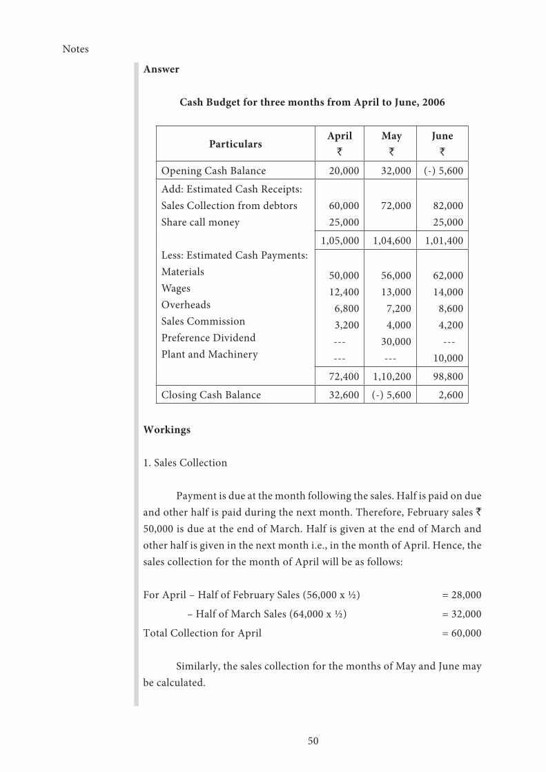
Answer

Cash Budget for three months from April to June, 2006

ParticularsApril

`

May `

June`

Opening Cash Balance 20,000 32,000 (-) 5,600

Add: Estimated Cash Receipts:Sales Collection from debtors Share call money

Less: Estimated Cash Payments:Materials Wages Overheads Sales Commission Preference DividendPlant and Machinery

60,00025,000

72,000 82,00025,000

1,05,000 1,04,600 1,01,400

50,00012,400

6,8003,200------

56,00013,000

7,2004,000

30,000---

62,00014,000

8,6004,200

---10,000

72,400 1,10,200 98,800

Closing Cash Balance 32,600 (-) 5,600 2,600

Workings

1. Sales Collection

Payment is due at the month following the sales. Half is paid on due and other half is paid during the next month. Therefore, February sales `

50,000 is due at the end of March. Half is given at the end of March and other half is given in the next month i.e., in the month of April. Hence, the sales collection for the month of April will be as follows:

For April – Half of February Sales (56,000 x ½) = 28,000

– Half of March Sales (64,000 x ½) = 32,000

Total Collection for April = 60,000

Similarly, the sales collection for the months of May and June may be calculated.

Notes

51

2. Materials and Overheads

These are paid in the following month. That is March is paid in April, April is paid in May and May is paid in June.

3. Sales Commission

It is paid in the following month. Therefore,

For April – 5% of March Sales (64,000 x 5 /100) = 3,200

For May – 5% of March Sales (80,000 x 5 /100) = 4,000

For April – 5% of March Sales (84,000 x 5 /100) = 4,200

Iv. Flexible Budget

A flexible budget consists of a series of budgets for different level of activity. Therefore, it varies with the level of activity attained. According to CIMA, London, A Flexible Budget is, ‘a budget designed to change in accordance with level of activity attained’. It is prepared by taking into account the fixed and variable elements of cost. This budget is more suitable when the forecasting of demand is uncertain.

Points to be remembered while preparing a flexible budget

1. Cost has to be classified into fixed and variable cost.2. Total fixed cost remains constant at any level of activity.3. Total Variable cost varies in the same proportion at which the level

of activity varies.4. Fixed and variable portion of Semi-variable cost is to be segregated.

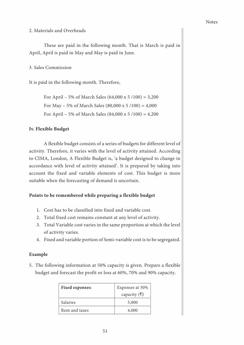
Example

5. The following information at 50% capacity is given. Prepare a flexible budget and forecast the profit or loss at 60%, 70% and 90% capacity.

Fixed expenses: Expenses at 50% capacity (`)

Salaries 5,000

Rent and taxes 4,000

Notes

52

Depreciation 6,000

Administrative expenses 7,000

Variable expenses:

Materials 20,000

Labour 25,000

Others 4,000

Semi-variable expenses:

Repairs 10,000

Indirect Labour 15,000

Others 9,000

It is estimated that fixed expenses will remain constant at all capacities. Semi-variable expenses will not change between 45% and 60% capacity, will rise by 10% between 60% and 75% capacity, a further increase of 5% when capacity crosses 75%.

Estimated sales at various levels of capacity are:

Capacity Sales (`)

60% 1,10,000 70% 1,30,000 90% 1,50,000

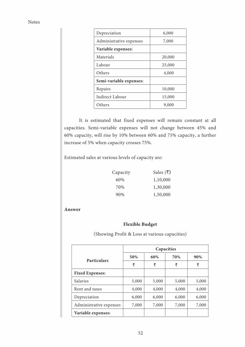
Answer

Flexible Budget

(Showing Profit & Loss at various capacities)

Particulars

Capacities

50% 60% 70% 90%

` ` ` `

Fixed Expenses:

Salaries 5,000 5,000 5,000 5,000

Rent and taxes 4,000 4,000 4,000 4,000

Depreciation 6,000 6,000 6,000 6,000

Administrative expenses 7,000 7,000 7,000 7,000

Variable expenses:

Notes

53

Materials 20,000 24,000 28,000 36,000

Labour 25,000 30,000 35,000 45,000

Others 4,000 4,800 5,600 7,200

Semi-variable expenses:

Repairs 10,000 10,000 11,000 11,500

Indirect Labour 15,000 15,000 16,500 17,250

Others 9,000 9,000 9,900 10,350

Total Cost 1,05,000 1,14,800 1,28,000 1,49,300

Profit (+) or Loss (-) (-) 4,800 (+) 2,000 (+) 700

Estimated Sales 1,10,000 1,30,000 1,50,000

Example

6. The following information relates to a flexible budget at 60% capacity. Find out the overhead costs at 50% and 70% capacity and also determine the overhead rates:

ParticularsExpenses at

60% capacity

Variable overheads: `

Indirect Labour 10,500

Indirect Materials 8,400

Semi-variable overheads:

Repair and Maintenance (70% fixed; 30% variable)

7,000

Electricity (50% fixed; 50% variable)

25,200

Fixed overheads:

Office expenses including salaries 70,000

Insurance 4,000

Depreciation 20,000

Estimated direct labour hours 1,20,000 hours

Notes

54

Answer

Flexible Budget

50 % Capacity

60% Capacity

70% Capacity

` ` `

Variable overheads:

Indirect Labour 8,750 10,500 12,250

Indirect Materials 7,000 8,400

Semi-variable overheads:

Repair and Maintenance (1) 6,650 7,000

Electricity (2) 23,100 25,200

Fixed overheads:

Office expenses including salaries 70,000 70,000 70,000

Insurance 4,000 4,000 4,000

Depreciation 20,000 20,000 20,000

Total overheads 1,39,500 1,45,100 1,50,700

Estimated direct labour hours 1,00,000 1,20,000 1,50,000

Overhead rate per hour (`) 1.395 1.21 1.077

Workings

1. The amount of Repairs and maintenance at 60% Capacity is `

7,000. Out of this, 70% (i.e ` 4,900) is fixed and remaining 30% (i.e ` 2,100) is variable. The fixed portion remains constant at all levels of capacities. Only the variable portion will change according to change in the level of activity. Therefore, the total amount of repairs and maintenance for 50% and 70% capacities are calculated as follows:

Repairs and maintenance 50% 60% 70%

Fixed (70%) Variable (30%)

4,9001,750

4,9002,100

4,9002,450

Total 6,650 7,000 7,350

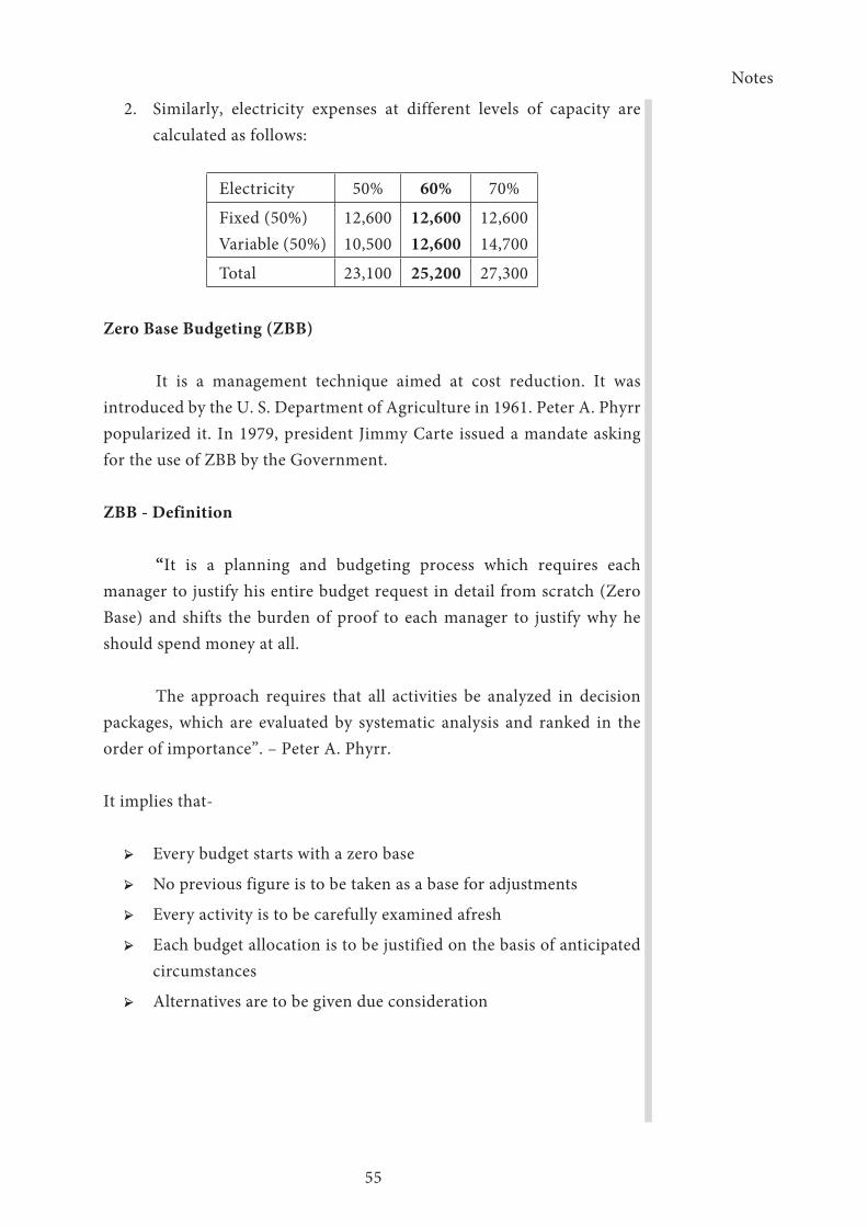
Notes

55

2. Similarly, electricity expenses at different levels of capacity are calculated as follows:

Electricity 50% 60% 70%

Fixed (50%) Variable (50%)

12,60010,500

12,60012,600

12,60014,700

Total 23,100 25,200 27,300

Zero Base Budgeting (ZBB)

It is a management technique aimed at cost reduction. It was introduced by the U. S. Department of Agriculture in 1961. Peter A. Phyrr popularized it. In 1979, president Jimmy Carte issued a mandate asking for the use of ZBB by the Government.

ZBB - Definition

“It is a planning and budgeting process which requires each manager to justify his entire budget request in detail from scratch (Zero Base) and shifts the burden of proof to each manager to justify why he should spend money at all.

The approach requires that all activities be analyzed in decision packages, which are evaluated by systematic analysis and ranked in the order of importance”. – Peter A. Phyrr.

It implies that-

➢ Every budget starts with a zero base

➢ No previous figure is to be taken as a base for adjustments

➢ Every activity is to be carefully examined afresh

➢ Each budget allocation is to be justified on the basis of anticipated circumstances

➢ Alternatives are to be given due consideration

Notes

56

Advantages of ZBB

1. Effective cost control can be achieved

2. Facilitates careful planning

3. Management by Objectives becomes a reality

4. Identifies uneconomical activities

5. Controls inefficiencies

6. Scarce resources are used judiciously

7. Examines each activity thoroughly

8. Controls wasteful expenditure

9. Integrates the management functions of planning and control

10. Reviews activities before allowing funds for them.

Performance Budgeting

It involves evaluation of the performance of the organization in the context of both specific as well as overall objectives of the organization. It provides a definite direction to each employee and a control mechanism to top management.

Definition

Performance Budgeting technique is the process of analyzing, identifying, simplifying and crystallizing specific performance objectives of a job to be achieved over a period of the job. The technique is characterized by its specific direction towards the business objectives of the organization. – The National Institute of Bank Management.

The responsibility for preparing the performance budget of each department lies on the respective departmental head. It requires preparation of performance reports. This report compares budget and actual data and shows any existing variances. To facilitate the preparation, the departmental head is supplied with the copy of the master budget appropriate to his function.

Notes

57

Master Budget

Master budget is a comprehensive plan which is prepared from and summarizes the functional budgets. The master budget embraces both operating decisions and financial decisions. When all budgets are ready, they can finally produce budgeted profit and loss account or income statement and budgeted balance sheet. Such results can be projected monthly, quarterly, half-yearly and at year end. When the budgeted profit falls short of target it may be reviewed and all budgets may be reworked to reach the target or to achieve a revised target approved by the budget committee.

****

Notes

58

Lesson 2.2 - Standard Costing

Standard: According to Prof. Erie L. Kolder, “Standard is a desired attainable objective, a performance, a goal, a model”.

Standard Cost: Standard cost is a predetermined estimate of cost to manufacture a single unit or a number of units during a future period.

The Chartered Institute of Management Accountants, London, defines “Standard Cost” as, “a pre-determined cost which is calculated from management’s standards of efficient operation and the relevant necessary expenditure. It may be used as a basis for price fixing and for cost control through variance analysis”.

Standard Costing: According to the Chartered Institute of Management Accountants, London Standard Costing is “the preparation and use of Standard Cost, their comparison with actual costs, and the analysis of variances to their causes and points of incidence”.

The study of standard cost comprises of:

1. Ascertainment and use of standard costs.

2. Comparison of actual costs with standard costs and measuring the variances.

3. Controlling costs by the variance analysis.

4. Reporting to management for taking proper action to maximize the efficiency.

Budgetary Control and Standard Costing

Both standard costing and budgetary control aim at maximum efficiency and managerial control. Budgetary control and standard costing have the common objective of controlling business operations by establishing pre-determined targets, measuring the actual performance and comparing it with the targets, for the purposes of having better efficiency

Notes

59

and of reducing costs. The two systems are said to be interrelated but they are not inter-dependent. The budgetary control system can function effectively even without the system of standard costing in operation but the vice-versa is not possible.

Standard Costing as a Controlling Technique

It is essential for management to have knowledge of costs so that decision can be effective. Management can control costs on information being provided to it. The technique of standard costing is used for building a proper budgeting and feedback system. The uses of standard costing to management are as follows.

1. Formulation of Price and Production Policies

Standard Costing acts as a valuable guide to management in the fixation of price and formulation production polices. It also assists management in the field of inventory pricing, product, product pricing profit planning and also in reporting to top management.

2. Comparison and Analysis of Data

Standard Costing provides a stable basis for comparison of actual with standard costs. It brings out the impact of external factors and internal causes on the cost and performance of the concern. Thus, it helps to take remedial action.

3. Cost Consciousness

An atmosphere of cost consciousness is created among the staff. Standard costing also provides incentive to workers for efficient performance.

4. Better Capacity to Anticipate

An effective budget can be formulated for the future by laving price knowledge of the deviations of actual costs from standard costs. Data are available at an early stage and the capacity to anticipate about changing conditions is developed.

Notes

60

5. Better Economy, Efficiency and Productivity

Men, machines and materials are more effectively utilized and thus benefits of economies can be reaped in business together with increased productivity.

6. Delegation of Authority and Responsibility

The net profit is analyzed and responsibility can be placed on the person in charge for any variations from the standards. It discloses adverse variations and particular cost centre can be held accountable. Thus, delegation of authority can be made by management to control the affairs in different departments.

7. Management by ‘Exception’

The principle of “management by exception’ can be applied in the business. This helps the management in concentrating its attention on cases which are off standard, i.e., below or above the standard set. A pattern is provided for the elimination of undesirable factors causing damage to the business.

Setting the Standard

While setting standard cost for operations, process or products, the following preliminaries must be gone through:

1. Establish Standard Committee comprising Purchase Manager, Personnel Manager, and Production Manager. The Cost Accountant coordinates the functions.

2. Study the existing costing system, cost records and forms in use.

3. A technical survey of the existing methods of production should be undertaken.

4. Determine the type of standard to be used.

5. Fix standard for each element of cost.

6. Determine standard costs of r each product.

7. Fix the responsibility for setting standards.

8. Account variances properly.

Notes

61

9. Ascertain the deviations by comparing the actual with standards.

10. Take necessary action to ensure that adverse variances are not repeated.

Determination of Standard Costs

The following preliminary steps are considered before setting standards:

(a) Establishment of cost centre

(b) Classification and codification of accounts

(c) Types of standards

(d) Setting the standards.

(a) Establishment of cost centre. For fixing responsibility and defining the lines of authority, cost centre is necessary. “A cost centre is a location, person or item of equipment (or group of these) for which costs may be ascertained and used of the purpose of cost control”. With the help of cost centre, the standards are prepared and the variances are analyzed.

(b) Classification and codification of accounts. Accounts are classified according to different items of expenses under suitable heading. Each heading may be given codes and symbols. Coding is useful for speedy collection and analysis.

(c) Types of standards. The different types of standards are given below:

(i) Basic standard. It is fixed and unaltered for an indefinite period for forward planning. According to I.C.M.A London, it is “an underlying standard from which a current standard can be developed”. From this basic standard, changes in current standard and actual standard can be measured.

(ii) Current standard. It is a short-term standard, as it is revised at regular intervals. I.C.M.A. London refers to it as “a standard which is established for use over a short period of time and is related to current conditions”. This standard is realistic and helpful to business. It is useful for cost control.

Notes

62

(iii) Normal standard. It is an average standard, and is based on normal conditions which prevail over a long period of a trade cycle. I.C.M.A defines it as “the average standard which, it is anticipated, can be attained over a future period of time, preferably long enough to cover one trade-cycle”. It is used for planning and decision making during the period of trade cycle to which it is related. It is very difficult to apply in practice.

(iv) Ideal standard. I.C.M.A. defines it as “the standard which can be attained under the most favorable condition possible”. It is fixed and needs a high degree of efficiency, best possible con-ditions of management and performance. Existing conditions and conditions capable of achievement should be taken into consideration. It is difficult to attain this ideal standard.

(v) Expected standard. It is a practical standard. I.C.M.A defines it as, “the standard which, it is anticipated, can be attained during a future specified budget period”. For setting this standard, due weightage is given for all the expected conditions. It is more realistic than the ideal standard.

(d) Setting the standards. After choosing the standard, the setting of standard is the work of the standard committee. The cost accountant has to supply the necessary cost figures and co-ordinate the activity committee. He must ensure that the setting standards are accurate.

Standards cost is determined for each element of the following costs.

(i) Direct Material cost. Standard material cost is equal to the standard quantity multiplied by the standard price. The setting of standard costs for direct materials involves

(a) Standard Material Quantity. For each product or part or the process, mechanical calculation or mechanical analysis is made. The allowance for normal wastage or loss must be fixed very carefully. Similarly, where different kinds of materials are used as a mix for a process, a standard material mix is determined to produce the desire quality product.

(b) Standard Material Price. Setting of material standard price is done by the cost accountant and the purchase manager. The

Notes

63

current standard is the desirable and effective for fixing the price. Normally one year is the period for fixation of standard price. If there are more fluctuations in prices, then revision of standard price is necessary. Before fixing the standard, the following points must be considered:

➢ Prices of materials in stock

➢ Price quoted by suppliers

➢ Trade and cash discounts received

➢ Future prices based upon statistical data

➢ Material price already contracted

(ii) Setting standard for Direct Labour. The standard labour cost is equal to the standard time for each operation multiplied by the standard wage rate. Setting of standard cost of direct labour involves:

(a) Fixation of standard time

(b) Fixation of standard rate

(a) Fixation of standard time: Standard time is fixed by time or motion study or past records or test runs or estimates. Labour time is fixed by the work study engineer. While fixing standard time, normal ideal time is allowed for fatigue, normal delays or other contingencies.

(b) Fixation of standard rate. With the help of the personnel manager, the accountant determines the standard rate. Fixation of standard rate is influenced by (i) Union’s policy (ii) Demand for labour (iii) Policy the be followed. (iv) Method of wage payment.

(iii) Setting standard for Overhead. Overheads are divided into fixed, variable and semi-variable. Standard overhead rate is determined on the basis of past records and future trend of prices. It is calculated for a unit or for an hour.

Standard variable overhead rate=

Standard variable overhead for the budge Period-----------------------------------------------------------Budgeted production units or budgeted hours for the

budgeted period (or some other base)

Notes

64

Standard fixed overhead rate=

Standard overheads for the budget period ------------------------------------------------------------Budgeted production units or budgeted hours for the

budgeted period (or some other base) Revision of Standards

Standard cost may be established for an indefinite period. There are no definite rules for the selection for a particular period. If the standards are fixed for a short period, it is expensive and frequent revision of standards will impair the utility and purpose for which standard is set.

At the same, if the standard is set for a longer period, it may not be useful particularly in the days of high inflation and large fluctuations of rates in case of materials and labour.

Standards have to be revised from time to time taking into consideration changing circumstances. The circumstances may change on account of technical innovations, changed market conditions, increase or decrease in plant capacity, developing new products or giving up unprofitable production lines. If variations from actual occur in practice, they may be due to controllable or uncontrollable causes. Standards should be revised only on account of those causes which are beyond the control of the management. Changes in product design, supply of labour and material, changes in market conditions for a long period, trade or cyclical variations would impel the management to revise the standards. The objective, while comparing the actual performance with the standard performance and revising standards, is to facilitate better control over costs and improve the overall working and profitability of the organization.

Apart from the above, basic standards are revised in the course of time under the following circumstances, when:

1. There are permanent changes in the method of production –designs and specifications.

2. Plant capacity is changed

3. There is a large variation between the standard and the actual.

Notes

65

Budgetary Control and Standard Costing

The systems of budgetary control and standard costing have the common objective of controlling business operations by establishing pre-determined targets, measuring the actual performance and comparing it with the targets, for the purposes of having better efficiency and of reducing costs. These two systems are said to be interrelated but they are not inter-dependent. The budgetary control system can function effectively even without the system of standard costing in operation but the vice-versa is not true. Usually, the two are used in conjunction with each other to have most fruitful results. The distinction between the two systems is mainly on account of the field or scope and technique of operation.

Budgeting Standard costing

1. Budgetary control is concerned with the operation of the business as a whole and hence its more extensive

1. Standard Costing is related with the control of the expenses and hence it is more intensive

2. Budget is a projection of financial accounts

2. Standard cost is the projection of cost accounts

3. It does not necessarily involve standardization of products.

3. It requires standardization of products.

4. Budgetary control can be adopted in part also.

4. It is not possible to operate this system in parts

5. Budgeting can be operated without standard costing.

5. Standard costing cannot exist with out budgeting.

6. Budgets determine the ceilings of expenses above which actual expenditure should not normally rise.

6. Standards are minimum targets which are to be attained by actual performance at specific efficiency level.

****

Notes

66

Lesson 2.3 - Variance Analysis

It involves the measurement of the deviation of actual performance form the intended performances. It is based on the principle of management by exception. The attention of management is drawn not only to the variation in monetary gain but also to the responsibility and causes for the same.

Favourable and Unfavourable Variances

Variances may be favorable (positive or credit) or unfavorable (or negative or adverse or debit) depending upon whether the actual cost is less or more than the standard cost.

Favorable variance: When the actual cost incurred is less than the standard cost, the deviation is known as favorable variance. The effect of the favorable variance increases the profit. It is also known as positive or credit variance.

Unfavorable variance: When the actual cost incurred is more than the standard cost, the variance is known as unfavorable or adverse variance. It refers to deviation causing the loss to the business. It is also known as negative or debit variance.

Controllable and Uncontrollable Variance

Variances may be controllable or uncontrollable, depending upon the controllability of the factors causing variances.

Controllable variance: It refers to a deviation caused by such factors which could be influenced by the executive action. For example, excess usage of materials, excess time taken by a worker, etc. When compared to the standard cost it is controllable as the responsibility can be fixed on the in-charge.

Notes

67

Uncontrollable variance: When variance is due to the factors beyond the control of the concerned person (or department), it is uncontrollable. For example, the wage rate increased on account of strike, government restrictions, change in market price etc. Only revision of standards is required to remove such in future.

Uses

The variance analysis is important tools of cost control and cost reduction and they generate an atmosphere of cost consciousness in the organization.

1. Comparison of actual with standard cost which reveals the efficiency or inefficiency of performance. The inefficiency or unfavorable variance is analyzed and immediate actions are taken.

2. It is a tool of cost control and cost reduction

3. It helps to apply the principle of management by exception.

4. It helps the management to maximize the profits by analyzing the variances into controllable and uncontrollable; the controllable variances are further analyzed so as to bring a cost reduction, indirectly more profit.

5. Future planning and programmes are based on the variance analysis.

6. Within the organization, a cost consciousness is created along with the team spirit.

Computation of Variances

The causes of variance are necessary to find remedial measures; and therefore a detailed study of variance analysis is essential. Variances can be found out with respect to all the elements of cost, i.e., direct material, direct labour and overheads. The following are the common variances, which are calculated by the management. Sub-divisions of variances in fact,d give detailed information to the management in order to control the cost.

Notes

68

1. Material variances

2. Labour variances

3. Overhead variances (a) variable (b) fixed

Material Variance

The following are the variances in the case of materials

a) Material Cost Variance (MCV). It is the difference between the stand-ard cost of direct materials specified for the output achieved and the actual cost of direct materials used. The standard cost of materials is computed by multiplying the standard price with the standard quan-tity for actual output; and the actual cost is computed by multiplying the actual price with the actual quantity. The formula is:

Material Cost Variance (or) MCV

(Standard cost of materials - Actual cost of materials used)

(or)

(Standard Quantity for actual output x Standard Price) - (Actual Quantity x Actual Rate) (or)

(SO x SP) - (AQ x AP)

b) Material Price Variance (MPV). Material price variance is that portion of the direct materials cost variance which is the difference between the standard price specified and the actual price paid for the direct materials used. The formula is:

Material Price Variance

(Actual Quantity consumed x Standard Price) – (Actual Quantity consumed x Actual Price) (or)

Actual Quantity consumed (Standard Price - Actual Price)

(or)

MPV= AQ (SP-AP)

c) Material Usage (Quantity) Variance (MUV). It is the deviation caused by the difference between the standards fixed and actual quantity used

Notes

69

for actual production at standard price. It is calculated by multiplying the difference between the standard quantity specified and the actual quantity used by the standard price.

Thus material usage variance is “that portion of the direct materials cost variance which is the difference between the standard quantity specified for the production achieved, whether completed or not, and the actual quantity used, both valued at standard prices”.

Material Usage or Quantity Variance

Standard Rate (Standard Quantity - Actual Quantity) (or)

MUV = SR (SQ-AQ)

d) Material Mix Variance (MMV). When two or more materials are used in the manufacture of a product, the difference between the standard composition and the actual composition of material mix is the material mix variance. The variance arises due to the change in the ratio of material and the standard ratio. The formula is:

Material Mix Variance = Standard Rate (Standard Mix – Actual Mix)

Standard is revised due to the shortage of a particular type of material.

The formula is:

MMV = Standard Rate (Revised Standard Quantity - Actual Quantity)Revised Standard Quantity (RSQ) =

Total weight of actual mix--------------------------------- x Standard Quantity

Total weight of standard mix

After finding out this revised standard mix it is multiplied by the revised standard cost of standard mix and then the standard cost of actual mix is subtracted form the result.

Notes

70

Example:1

The standard cost of material for manufacturing a unit a particular product is estimated as 16kg of raw materials @ ` 1 per kg.

On completion of the unit, it was found that 20kg. of raw material costing ` 1.50 per kg. has been consumed. Compute Material Variances.

Answer

MCV = (SQ x SP) - (AQ x AP) = (16 x ` 1) - (20 x ` 1.50)

= ` 16 - ` 30

= ` 14 (Adverse)

MPV = (SP – AP) x AQ = (1 – 1.50) x 20

= ` 10 (Adverse)

MUV = (SQ – AQ) x SP = (16 – 20) x 1

= ` 4 (Adverse)

Example:2

Calculate the materials mix variance from the following:

Material Standard Actual A 90 units at ` 12 each 100 units at ` 12 each B 60 units at ` 15 each 50 units at ` 16 each

Answer:

Material Standard Actual

Qty Rate Amount Qty Rate Amount

AB

90 12 1080 60 15 900

100 12 1200 50 16 800

150 1980 150 2000

MMV = SR (SQ-AQ)

Material ‘A’: MMV = ` 12 (90-100)

= ` 12 x10

= ` 120(A)

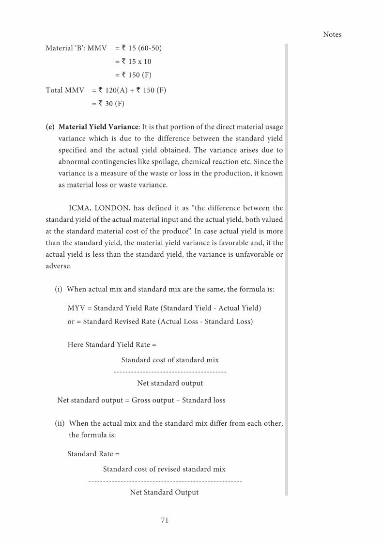
Notes

71

Material ‘B’: MMV = ` 15 (60-50)

= ` 15 x 10

= ` 150 (F)

Total MMV = ` 120(A) + ` 150 (F)

= ` 30 (F)

(e) Material Yield Variance: It is that portion of the direct material usage variance which is due to the difference between the standard yield specified and the actual yield obtained. The variance arises due to abnormal contingencies like spoilage, chemical reaction etc. Since the variance is a measure of the waste or loss in the production, it known as material loss or waste variance.

ICMA, LONDON, has defined it as “the difference between the standard yield of the actual material input and the actual yield, both valued at the standard material cost of the produce”. In case actual yield is more than the standard yield, the material yield variance is favorable and, if the actual yield is less than the standard yield, the variance is unfavorable or adverse.

(i) When actual mix and standard mix are the same, the formula is:

MYV = Standard Yield Rate (Standard Yield - Actual Yield)

or = Standard Revised Rate (Actual Loss - Standard Loss)

Here Standard Yield Rate =

Standard cost of standard mix ---------------------------------------

Net standard output

Net standard output = Gross output – Standard loss

(ii) When the actual mix and the standard mix differ from each other, the formula is:

Standard Rate =

Standard cost of revised standard mix -----------------------------------------------------

Net Standard Output

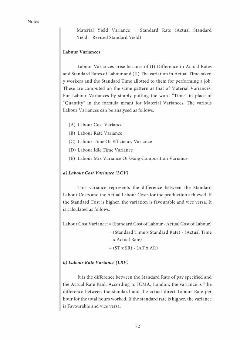
Notes

72

Material Yield Variance = Standard Rate (Actual Standard Yield – Revised Standard Yield)

Labour Variances

Labour Variances arise because of (I) Difference in Actual Rates and Standard Rates of Labour and (II) The variation in Actual Time taken y workers and the Standard Time allotted to them for performing a job. These are computed on the same pattern as that of Material Variances. For Labour Variances by simply putting the word “Time” in place of “Quantity” in the formula meant for Material Variances. The various Labour Variances can be analysed as follows:

(A) Labour Cost Variance

(B) Labour Rate Variance

(C) Labour Time Or Efficiency Variance

(D) Labour Idle Time Variance

(E) Labour Mix Variance Or Gang Composition Variance

a) Labour Cost Variance (LCV)

This variance represents the difference between the Standard Labour Costs and the Actual Labour Costs for the production achieved. If the Standard Cost is higher, the variation is favourable and vice versa. It is calculated as follows:

Labour Cost Variance: = (Standard Cost of Labour - Actual Cost of Labour)

= (Standard Time x Standard Rate) - (Actual Time x Actual Rate)

= (ST x SR) - (AT x AR)

b) Labour Rate Variance (LRV)

It is the difference between the Standard Rate of pay specified and the Actual Rate Paid. According to ICMA, London, the variance is “the difference between the standard and the actual direct Labour Rate per hour for the total hours worked. If the standard rate is higher, the variance is Favourable and vice versa.

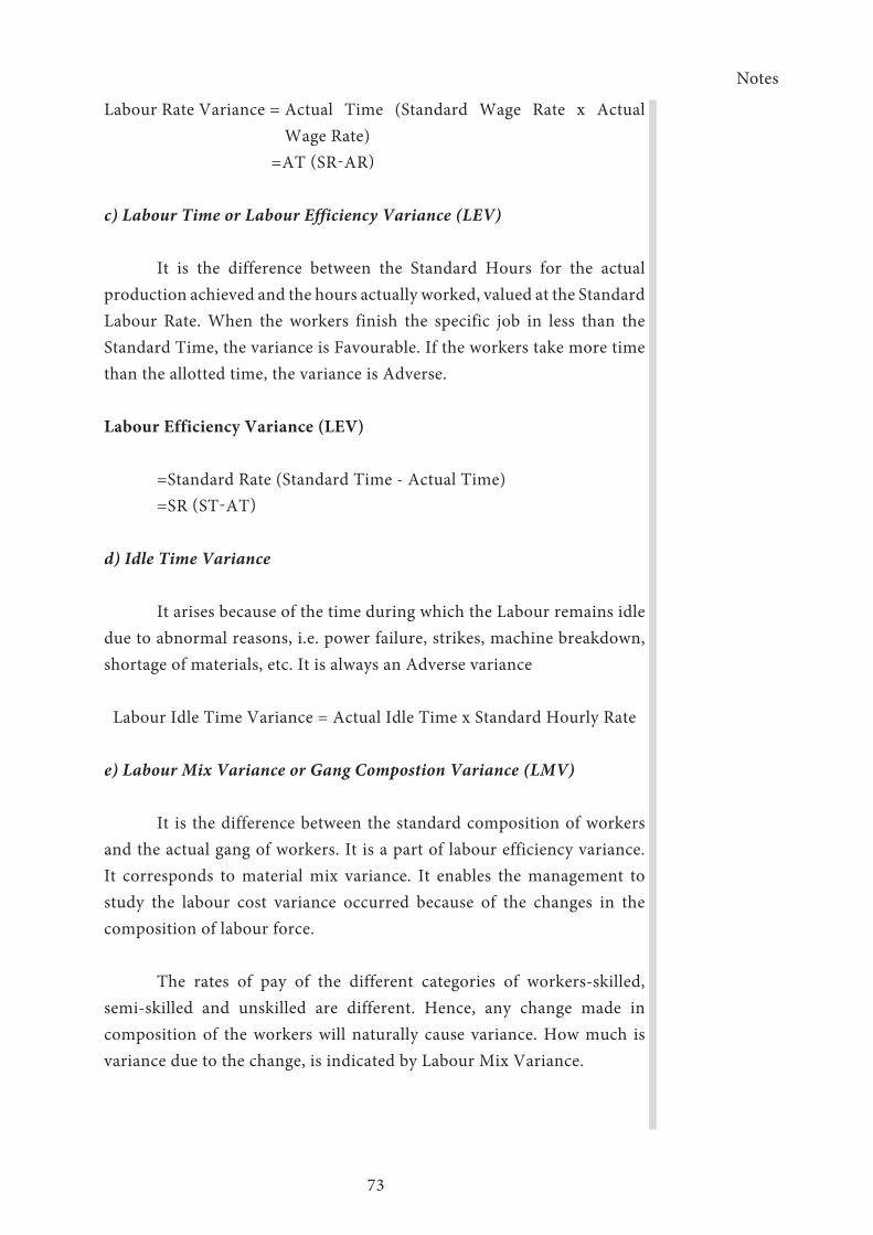
Notes

73

Labour Rate Variance = Actual Time (Standard Wage Rate x Actual Wage Rate)

=AT (SR-AR)

c) Labour Time or Labour Efficiency Variance (LEV)

It is the difference between the Standard Hours for the actual production achieved and the hours actually worked, valued at the Standard Labour Rate. When the workers finish the specific job in less than the Standard Time, the variance is Favourable. If the workers take more time than the allotted time, the variance is Adverse.

Labour Efficiency Variance (LEV)

=Standard Rate (Standard Time - Actual Time) =SR (ST-AT)

d) Idle Time Variance

It arises because of the time during which the Labour remains idle due to abnormal reasons, i.e. power failure, strikes, machine breakdown, shortage of materials, etc. It is always an Adverse variance

Labour Idle Time Variance = Actual Idle Time x Standard Hourly Rate

e) Labour Mix Variance or Gang Compostion Variance (LMV)

It is the difference between the standard composition of workers and the actual gang of workers. It is a part of labour efficiency variance. It corresponds to material mix variance. It enables the management to study the labour cost variance occurred because of the changes in the composition of labour force.

The rates of pay of the different categories of workers-skilled, semi-skilled and unskilled are different. Hence, any change made in composition of the workers will naturally cause variance. How much is variance due to the change, is indicated by Labour Mix Variance.

Notes

74

(i) When the total hours i.e. time of the standard composition and actual composition of workers does not differ the formula is:

Labour Mix variance= (Standard Cost of Standard Mix) - (Standard cost of Actual Mix)

(ii) When the total hours i.e. time of the standard composition and actual composition of workers differs, the formula is:

Labour Mix Variance

Total Time of Actual mix………………………..…. x Std cost of Std. mix) - (Std. cost of Actual Mix)Total Time of Standard Mix

If, on account of short availability of some category of workers, the standard composition is itself revised, then Labour Mix Variance will be calculated by taking revised standard mix in place of standard mix.

Labour Yield Variance (LYV)

It is just like Material Yield Variance. It is the difference between the standard labour output and actual output of yield. It is calculated as below:

Labour Yield Variance

= Standard cost per unit {Standard production of Actual mix - Actual Production}

Overhead Variance

Overhead Cost Variance

It is the difference between standard overheads for actual output i.e. Recovered Overheads and Actual Overheads. It is the total of both fixed and variable overhead variances. The variable overheads are those costs which tend to vary directly in proportion to changes in the volume of production. Fixed overheads consist of costs which are not subject to

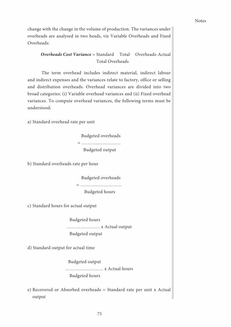
Notes

75

change with the change in the volume of production. The variances under overheads are analysed in two heads, viz Variable Overheads and Fixed Overheads:

Overheads Cost Variance = Standard Total Overheads-Actual Total Overheads

The term overhead includes indirect material, indirect labour and indirect expenses and the variances relate to factory, office or selling and distribution overheads. Overhead variances are divided into two broad categories: (i) Variable overhead variances and (ii) Fixed overhead variances. To compute overhead variances, the following terms must be understood:

a) Standard overhead rate per unit

Budgeted overheads= ………..……………

Budgeted output

b) Standard overheads rate per hour

Budgeted overheads= ………………………

Budgeted hours

c) Standard hours for actual output

Budgeted hours…………………. x Actual output

Budgeted output

d) Standard output for actual time

Budgeted output……………………. x Actual hours

Budgeted hours

e) Recovered or Absorbed overheads = Standard rate per unit x Actual output

Notes

76

f) Budgeted overheads = Standard rate per unit x budgeted output

g) Standard overheads = Standard rate per unit x Standard output for actual time

h) Actual overheads = Actual rate per unit x Actual output

Variable Overhead Variance

Variable cost varies in proportion to the level of output, while the cost is fixed per unit. As such the standard cost per unit of these overheads remains the same irrespective of the level of output attained. As the volume does not affect the variable cost per unit or per hour, the only factors leading to difference is price. It results due to the change in the expenditure incurred.

(i) Variable Overhead Expenditure Variance

It is the difference between actual variable overhead expenditure incurred and the standard variable overheads set in for a particular period. The formula is:-

{Actual Hours Worked x Standard Variable Overhead Rate per hour}-Actual Variable overheads

(ii) Variable Overhead Efficiency Variance

It shows the effect of change in labour efficiency on variable overheads recovery. The formula is:- Standard Rate (Standard Quantity-Actual Quantity)

Standard Overhead Rate = (Standard Time for Actual output- Actual Time)

(iii) Variable Overhead Variance

It is divided into two: Overhead Expenditure Variance and Overhead Efficiency Variance. The formula is:-

Variable overhead Expenditure Variance + Variable overhead Efficiency variance

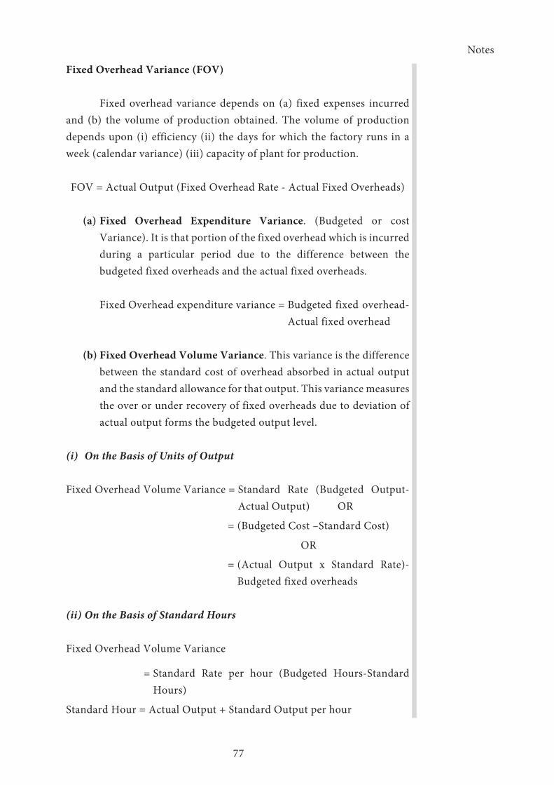
Notes

77

Fixed Overhead Variance (FOV)

Fixed overhead variance depends on (a) fixed expenses incurred and (b) the volume of production obtained. The volume of production depends upon (i) efficiency (ii) the days for which the factory runs in a week (calendar variance) (iii) capacity of plant for production.

FOV = Actual Output (Fixed Overhead Rate - Actual Fixed Overheads)

(a) Fixed Overhead Expenditure Variance. (Budgeted or cost Variance). It is that portion of the fixed overhead which is incurred during a particular period due to the difference between the budgeted fixed overheads and the actual fixed overheads.

Fixed Overhead expenditure variance = Budgeted fixed overhead-Actual fixed overhead

(b) Fixed Overhead Volume Variance. This variance is the difference between the standard cost of overhead absorbed in actual output and the standard allowance for that output. This variance measures the over or under recovery of fixed overheads due to deviation of actual output forms the budgeted output level.

(i) On the Basis of Units of Output

Fixed Overhead Volume Variance = Standard Rate (Budgeted Output-Actual Output) OR

= (Budgeted Cost –Standard Cost)

OR

= (Actual Output x Standard Rate)-Budgeted fixed overheads

(ii) On the Basis of Standard Hours

Fixed Overhead Volume Variance

= Standard Rate per hour (Budgeted Hours-Standard Hours)

Standard Hour = Actual Output + Standard Output per hour

Notes

78

Sales Variances

Sales are affected by two factors (i) the selling price and (ii) the quantity of sales the variations in the standards set and actual for the purpose may be mainly due to change in market trends. Normally, if the selling price increases, the volume of sales will be lower than the standard. It is to be kept in mind that higher price is to be seen as a favorable variance (higher price paid for material will be an adverse variance) and lower volume of sales is to be looked as an unfavorable (in case of materials, it is the other way around, i.e. lower usage of materials than the standard causes a favorable variance). It is well known that demand and supply position in the market decide the quantity of sales as well as the selling price. The variations may be on account of control lab: as well as non-controllable factors.

Sales Value Variance

The difference between budgeted sales and actual sales results in Sales Value variance.

The Formula is:

Sales Value Variance = Actual value of sales – Standard value of sales

Sales Price Variance

It is on account of the difference in actual selling price and the standard selling price for actual quantity of sales. The formula is:

Sales price variance = Actual Quantity Sold (Actual price-Standard price)

Sales Volume Variance

Budgeted sales may be different from the standard sales. In other words, budgeted quantity of sales at standard price may vary from the actual quantity of sales at standard prices. Thus, the variance is a result of difference in budgeted and actual quantities of goods sold. The formula is:

Sales volume variance = Standard price (Actual units – Standard units)

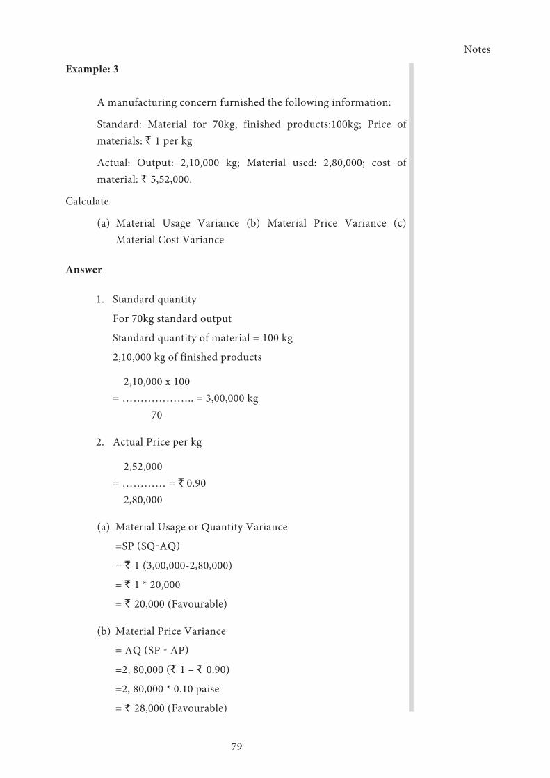
Notes

79

Example: 3

A manufacturing concern furnished the following information:

Standard: Material for 70kg, finished products:100kg; Price of materials: ` 1 per kg

Actual: Output: 2,10,000 kg; Material used: 2,80,000; cost of material: ` 5,52,000.

Calculate

(a) Material Usage Variance (b) Material Price Variance (c) Material Cost Variance

Answer

1. Standard quantity

For 70kg standard output

Standard quantity of material = 100 kg

2,10,000 kg of finished products

2,10,000 x 100= ……………….. = 3,00,000 kg 70

2. Actual Price per kg

2,52,000= ………… = ` 0.90 2,80,000

(a) Material Usage or Quantity Variance

=SP (SQ-AQ)

= ` 1 (3,00,000-2,80,000)

= ` 1 * 20,000

= ` 20,000 (Favourable)

(b) Material Price Variance

= AQ (SP - AP)

=2, 80,000 (` 1 – ` 0.90)

=2, 80,000 * 0.10 paise

= ` 28,000 (Favourable)

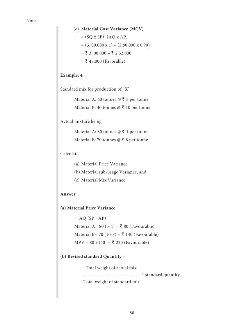
Notes

80

(c) Material Cost Variance (MCV)

= (SQ x SP)–(AQ x AP)

= (3, 00,000 x 1) – (2,80,000 x 0.90)

= ` 3, 00,000 – ` 2,52,000

= ` 48,000 (Favorable)

Example: 4

Standard mix for production of “X’

Material A: 60 tonnes @ ` 5 per tonne

Material B: 40 tonnes @ ` 10 per tonne

Actual mixture being:

Material A: 80 tonnes @ ` 4 per tonne

Material B: 70 tonnes @ ` 8 per tonne.

Calculate

(a) Material Price Variance

(b) Material sub-usage Variance, and

(c) Material Mix Variance

Answer

(a) Material Price Variance

= AQ (SP - AP)

Material A= 80 (5-4) = ` 80 (Favourable)

Material B= 70 (10-8) = ` 140 (Favourable)

MPV = 80 +140 -= ` 220 (Favourable)

(b) Revised standard Quantity =

Total weight of actual mix--------------------------------- * standard quantity

Total weight of standard mix

Notes

81

RSQ for material ‘A’

150= .…... * 60 = 90 tonnes

100

RSQ for material ‘B’

150= .…... * 40 = 60 tonnes

100

Material sub usage (Revised usage) Variance =

Standard Price (Standard. Quantity – Revised Standard Quantity)

RUV for material ‘A’= 5(60-90) = 150 (Adverse)

RUV for material ‘B’ = 10(40-90) = 200(Adverse)

MRV = 150+200= ` 350 (Adverse) Material Mix Variance = Standard Rate x (Revised std. Quantity -

Actual qty.)

MVV for material ‘A’= 5(90-80) =50 (Adverse)

MVV for material ‘B’= 10(60-70) =100 (Adverse)

MVV=50-100=-50=` 540 (Adverse)

Example: 5

Vinak Ltd. produces an article by blending two basic raw materials. It operates a standard costing system and the following standards have been set for new materials.

Material Standard Mix Standard price per kg A 40% ` 4.00 B 60% ` 3.00

The standard loss in processing is 15%

During April 1994 the company produced 1700 kgs of finished output. The position of stocks and purchases for the month of April 1994 is as under:

Notes

82

Material Stock on Stock on Purchased during April 1994 1-4-94 30-4-94 Kgs Kgs Kgs KgsA 35 5 800 3400B 40 50 1200 3000

Calculate: Material Price Variances, Material Usage Variances, Material yield variances, Material Mix Variances and Total Material Cost Variances.

Answer

Finished output 1,700 kgs. Standard Loss in processing 15%.

Therefore, input is

100 1,700 x …….. = 2000kgs

85

For an input of 2,000 kgs., the standard cost will be as follows

A - 40% of 2000 = 800 kgs. at ` 4.00 = ` 3,200 B - 60% of 2,000 =1,200 kgs at ` 3.00 = ` 3,600 …………. …………. 2,000kgs ` 6,800

Loss 15% 300kgs - …………. ………….

Finished

1,700 kgs ` 6,800output

6,800Standard Yield Rate =………= ` 4 per kg

1,700

Actual Costs

A - 35+800-5 = 830kgs. consumed 35 x 4 (assumed) = ` 140.00 795 x 4.25 (purchase price) = ` 3,378.75 ……………. ` 3,518.75

Notes

83

B 40 + 1,200 - 5 0=1190 kgs. consumed 40 x 3 (assumed) = 120.00

1150 x 2.50(purchase price) = 2,875.00 ……...….. ………….Total 2,020 6,513.75Less: Loss 320 _ ……...….. ………….Finished output 1,700 6,513.75

Material Price Variance = AQ (SP-AP)

A = 830 x 4 = 3,320 - 3,518.75 = ` 198.75 (A)B = 1,190 x 3=3,570 - 2,995 = ` 575.00 (F) …………….. ` 376.25 (F)

………………

Material Usage Variance = SP(SQ-AQ)

A = 4 (800-830) = 120(A)B= 3 (1,200-1,190) = 30(F) ………. ` 90(A) ……….

Material Yield Variance = SYR* (AY-SY)

= 4(1,700 - 1,717) = 68(A)If SY For 2,000 kgs. input SY = 1,700Then, For 2,020 kgs. input SY = ? 2,020 = ………. x 1,700 = 1,717 kgs} 2,000

Material Mix Variance = SP (RSQ-AQ)

Revised standard quantity=

Total weight of actual mix---------------------------------- x Standard Quantity

Total weight of standard mix

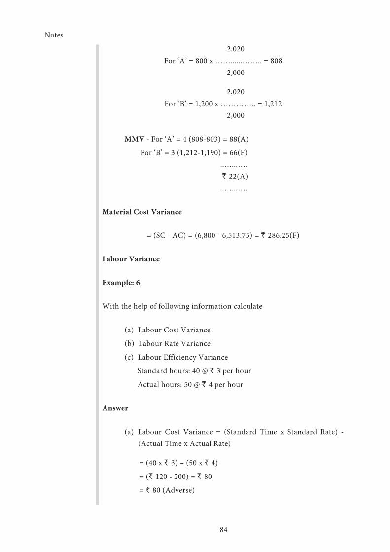
Notes

84

2.020For ‘A’ = 800 x ……......…….. = 808

2,000

2,020For ‘B’ = 1,200 x ………….. = 1,212

2,000 MMV - For ‘A’ = 4 (808-803) = 88(A)

For ‘B’ = 3 (1,212-1,190) = 66(F) ..…...…. ` 22(A) ..…...….

Material Cost Variance

= (SC - AC) = (6,800 - 6,513.75) = ` 286.25(F)

Labour Variance

Example: 6

With the help of following information calculate

(a) Labour Cost Variance

(b) Labour Rate Variance

(c) Labour Efficiency Variance

Standard hours: 40 @ ` 3 per hour

Actual hours: 50 @ ` 4 per hour

Answer

(a) Labour Cost Variance = (Standard Time x Standard Rate) - (Actual Time x Actual Rate)

= (40 x ` 3) – (50 x ` 4)

= (` 120 - 200) = ` 80

= ` 80 (Adverse)

Notes

85

(b) Labour Rate Variance = Actual Time (Standard Rate x Actual Rate)

= 50 (`3 - `4) = `50

= `50 (Adverse)

(c) Labour Efficiency Variance = Standard Rate (Standard Time-Actual Time)

= `3 (40 - 50) = ` 30

= `30 (Adverse)

Example; 7

The Labour budget of a company for a week is as follows:

20 skilled men @ 50 paise per hour for 40 hours = 400

40 skilled men @ 30 paise per hour for 40 hours = 480 ….. 880

…..

The actual labour force was used as follows:

30 skilled men @ 50 paise per hour for 40 hours = 600

30 skilled men @ 35 paise per hour for 40 hours = 420 …..... 1,020

Analyses labour variances.

Answer

1. Labour Rate Variance = AT (SR - AR)

(a) Skilled men = 1,200 (` 50 - ` 50) = 0

(b) Unskilled men = 1,200 (` 30 - ` 35) = ` 60 (A)

2. Labour Mix variance = SR (ST - AT)

(a) Skilled men = ` 0.50 (800 -1200) = ` 200 (A)

(b) Unskilled men = ` 0.30 (1600 - 1200) = ` 120 (F)

Total Labour Cost Variance = Standard labour cost - Actual cost = 880 - 1020 = 140 (A)

Notes

86

Example; 8

Standard labour hours and rate for production of Article A are given below:

Hrs. Rate (`) Total

Skilled workerUnskilled workerSemi-skilled worker

584

1.50 per hour0.50 per hour0.75 per hour

7.504.003.00

Actual data Rate per hour Total

Articles produced 1,000 unitsSkilled worker 4,500 hrsUnskilled worker 10,000 hrsSemi skilled worker 4,200 hrs

2.000.450.75

9,0004,5003,150

Calculate: Labour Cost Variance, Labour Rate Variance, Labour Efficiency Variance and Labour Mix Variance

Answer

(a) Labour Cost Variance

=(Standard Time x Standard Rate)-(Actual Time x Actual Rate)

Standard Time for Actual Production =Actual Units x ST.

Skilled Worker = 1,000 x 5 = 5000 Hrs.

Unskilled worker = 1,000 x 8 = 8,000 Hrs.

Semi-skilled worker = 1,000 x 4 = 4,000 Hrs.

Labour Cost Variance

Skilled worker = (5000 x ` 1.50) – (4,500 x 2)

= ` 7,500 – ` 9,000 = ` 1,500 (A)

Unskilled worker = ` (8,000 x ` 0.50) – (10,000 x 0.45)

= 4,000 - 4,500 = ` 500 (A)

Semi skilled worker = (4,000 x ` 0.75) – (4,200 x ` 0.75)

= 3,000-3,150) = ` 150 (A)

Total Labour Cost Variance = ` 2150 (A)

Notes

87

(b) Labour Rate Variance = Actual Time (Standard Rate x Actual Rate)

Skilled worker = 4500 (1.50 - 2) = ` 2250 (A)

Unskilled worker = ` 4,200 (0.75 – 0.75) = Nil

Semi skilled worker = 1,000 (0.50 - 0.45) = ` 500 (F)

Total Labour Rate Variance = ` 1,750 (A)

(c) Labour mix variance: = SR (Revised std. Mix of Actual hours worked) – Actual Mix

Revised std. Mix of Actual hours worked

Std Mix = …………………… x Total Actual Hrs. Total Std. Hours

5,000Skilled worker = …………… x 18,700 = 5,500 Hrs 17,000

8,000Unskilled worker = …………… x 18,700 = 8,800 Hrs. 17,000

4,000Semi skilled worker = …………… x 18,700 = 4,400 Hrs 17,000

Labour Mix Variance

Skilled worker = 1.50 (5,500 - 4,500) = ` 1,500 (F)

Unskilled worker = 0.50 (8,800 - 10,000) = ` 600 (A)

Semi skilled worker = 0.75 (4,400 - 4,200) = ` 150 (F)

Total Labour Mix Variance = ` 1050 (F)

Notes

88

(d) Labour Efficiency Variance = SR (ST for Actual output – Revised Std. Hrs)

Skilled worker = 1.50 (5,000 - 5,500) = ` 750 (A)

Unskilled worker = 0.50 (8,000 - 8,800) = ` 400 (A)

Semi skilled worker = 0.75 (4,000 - 4,400) = ` 300 (A)

Total Labour Efficiency Variance = `, 450 (A)

Overhead Variance

Example: 9

S.V. Ltd has furnished you the following data:

Budget Actual July 1994

No. of working days 25 27

Production in units 20,000 22,000

Fixed overheads ` 30,000 ` 31,000

Budgeted fixed overhead rate is ` 1 per hour. In July 1994, the actual hours worked were 31,500.

Calculate the following variance: (i) Efficiency Variance (ii) Capacity variance (iii) Volume variance (iv) Expenditure variance and (v) Total overhead variance.

Answer

Budgeted overhead Recovered overhead = …………….……… x Actual output Budgeted output

30,000 = ……….. x 22,000 20,000

= 33,000

Notes

89

i. Efficiency Variance = Standard Rate per hour (Standard hours for actual production – Actual hours)

= ` 1 x (33,000 – 31,500)

= ` 1,500 (F)

ii. Capacity Variance = Standard Rate per hour x (Actual hours - Budgeted hours)

= Standard overheads - Budgeted overheads = ` 1 x (31,500 – 30,000)

= ` 1500 (F)

iii. Volume variance = Recovered overhead – Budgeted overheads

= ` 33,000 – ` 30,000

= ` 3,000 (F)

iv. Expenditure variance = Budgeted overheads – Actual overheads

= ` 30,000 – ` 31,000

= ` 1,000 (A)

v. Total overhead variance = Recovered overhead – Actual overheads

= ` 33,000 – ` 31,000

= ` 2,000 (F)

Example: 10

Vinak Ltd.has furnished you the following for the month of August 1994.

Budget Actual

Output (Units)HoursFixed hoursVariable overheadWorking days

30,00030,000

`45,000`60,000

25

32,50033,00050,00068,000

26

Calculate the variances.

Notes

90

Answer

Standard Overhead Rate per Unit

Budgeted Overheads = ………….………….. Budgeted Output

30,000 = …………. = 1 hours 30,000

Total standard overhead rate per hour

Budgeted overheads = ………….………….. Budgeted hours

1,05,000 = …………. = ` 3.50 per hour 30,000

Standard fixed overhead rate per hour

Budgeted fixed overheads = ……………………..…….. Budgeted hours

45,000 = …………. = ` 1.50 30,000

Standard variable overhead rate per hour

Budgeted variable overheads = ………………………………. Budgeted hours

60,000 = …………. = ` 2 30,000

Notes

91

Overhead cost variance = Recovered overheads – Actual overheads

Recovered overhead = Actual output x Standard Rate per unit

= 32,500 x ` 3.50 = ` 1,13,750

Overhead cost variance = 1,13,750 – 1,18,000

= ` 4,250 (A)

Variable overhead cost variance = Recovered overheads – Actual overheads

= 32,500 hrs x ` 2 – ` 68,000

= ` 3,000 (A)

Fixed overhead cost variance = Recovered overheads – Actual overheads

= 32,500 hrs x ` 1.50 – ` 50,000

= 48,750 – 50,000

= ` 1,250 (A)

Expenditure variance = Budgeted overheads – Actual overheads

= ` 45,000 – ` 50,000

= ` 5000 (A)

Volume variance = Recovered overheads- Budgeted overheads

= 32500 hrs x ` 1.50 – 45,000

= 48,750 – 45,000

= ` 3,750 (F)

Efficiency variance = Recovered overheads- standard overheads

OR

Standard rate = (Standard hours for actual output – Actual hours)

= 1.50 (32,500 – 33,000)

= ` 750 (A)

Capacity variance = standard overheads – Budgeted overheads

Or

= Standard Rate (Actual hours - Budgeted hours)

= ` 1.50 (33,000 – 30,000)

= ` 4,500 (F)

Notes

92

Calendar variance = Extra / Deficit hours worked x Standard Rate.

One extra day has been worked.

.. The Total number of extra hours worked

30,000= ……….. = 1,200

25

= 1,200 x 1.50 = ` 1,800 (F)

Note

1. (F) – Favourable; (A) – Adverse (or) Unfavaourable

2. When Standard is more than the Actual, it is favourable variance

3. When Actual is more than the Standard, it is unfavourable or adverse variance

4. In place of ‘Time’, the term ‘Hours’ may also be used.

Disposal of Variances

Cost variances are disposed of in one of the following ways:

1. Transfer to profit and loss account, keeping work-in-progress, finished goods and cost of sales at standard cost.

2. Transfer to cost of sales, thus practically converting the standard cost of sales into actual cost of sales.

3. Prorating to cost of sales and inventories, either on the basis of units or value, so that both the inventories and cost of goods sold will be shown at actual costs.

Computation of Sales Variances

Example: 11

The budgeted and actual sales for a period in respect of two products are as follows:

Notes

93

Product Budgeted Actual

Qty (Units)

Price (`)

Value (`)

Qty (Units)

Price (`)

Value (`)

A 500 2 1700 700 3 3100

B 700 3 3100 500 2 1700

Find out sales variance

Solution

(i) Sales value variance = Actual sales – Standard sales

Total actual value = 3100+1700 = 4800

Total standard value = 1700+3100=4800

Sales value variance = 4800-4800 = Nil

(ii) Sales price variance = Actual Quantity Sold (Actual price-Standard price)

Product A 700 (3 - 2) = 700 (F)

Product B 500 (2 - 3) = 500 (A) --------- 200 (F) ---------

(iii) Sales volume variance = Standard price (Actual units – Standard units)

Product A 2 (700 - 500) = 400 (F)

Product B 3 (500 - 700) = 600 (A) --------- 200 (A) --------- F =Favorable A= Adverse

From the following data, calculate sales variances with an assumption that products are homogenous in nature.

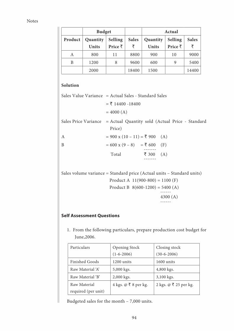
Notes

94

Budget Actual

Product Quantity Units

Selling Price `

Sales`

Quantity Units

Selling Price `

Sales`

A 800 11 8800 900 10 9000

B 1200 8 9600 600 9 5400

2000 18400 1500 14400

Solution

Sales Value Variance = Actual Sales - Standard Sales

= ` 14400 -18400

= 4000 (A)

Sales Price Variance = Actual Quantity sold (Actual Price - Standard Price)

A = 900 x (10 – 11) = ` 900 (A)

B = 600 x (9 – 8) = ` 600 (F) ------- Total ` 300 (A) -------

Sales volume variance = Standard price (Actual units – Standard units) Product A 11(900-800) = 1100 (F)

Product B 8(600-1200) = 5400 (A) ------ 4300 (A) ------

Self Assessment Questions

1. From the following particulars, prepare production cost budget for June,2006.

Particulars Opening Stock(1-6-2006)

Closing stock(30-6-2006)

Finished Goods 1200 units 1600 units

Raw Material ‘A’ 5,000 kgs. 4,800 kgs.

Raw Material ‘B’ 2,000 kgs. 3,100 kgs.

Raw Material required (per unit)

4 kgs. @ ` 8 per kg. 2 kgs. @ ` 25 per kg.

Budgeted sales for the month – 7,000 units.

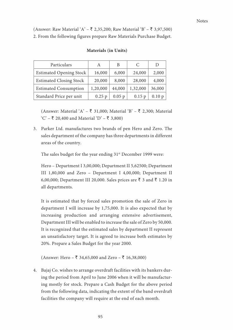
Notes

95

(Answer: Raw Material ‘A’ – ` 2,35,200; Raw Material ‘B’ – ` 3,97,500)2. From the following figures prepare Raw Materials Purchase Budget.

Materials (in Units)

Particulars A B C D

Estimated Opening Stock 16,000 6,000 24,000 2,000

Estimated Closing Stock 20,000 8,000 28,000 4,000

Estimated Consumption 1,20,000 44,000 1,32,000 36,000

Standard Price per unit 0.25 p 0.05 p 0.15 p 0.10 p

(Answer: Material ‘A’ – ` 31,000; Material ‘B’ – ` 2,300; Material ‘C’ – ` 20,400 and Material ‘D’ – ` 3,800)

3. Parker Ltd. manufactures two brands of pen Hero and Zero. The sales department of the company has three departments in different areas of the country.

The sales budget for the year ending 31st December 1999 were:

Hero – Department I 3,00,000; Department II 5,62500; Department III 1,80,000 and Zero – Department I 4,00,000; Department II 6,00,000; Department III 20,000. Sales prices are ` 3 and ` 1.20 in all departments.

It is estimated that by forced sales promotion the sale of Zero in department I will increase by 1,75,000. It is also expected that by increasing production and arranging extensive advertisement, Department III will be enabled to increase the sale of Zero by 50,000. It is recognized that the estimated sales by department II represent an unsatisfactory target. It is agreed to increase both estimates by 20%. Prepare a Sales Budget for the year 2000.

(Answer: Hero – ` 34,65,000 and Zero – ` 16,38,000)

4. Bajaj Co. wishes to arrange overdraft facilities with its bankers dur-ing the period from April to June 2006 when it will be manufactur-ing mostly for stock. Prepare a Cash Budget for the above period from the following data, indicating the extent of the band overdraft facilities the company will require at the end of each month.

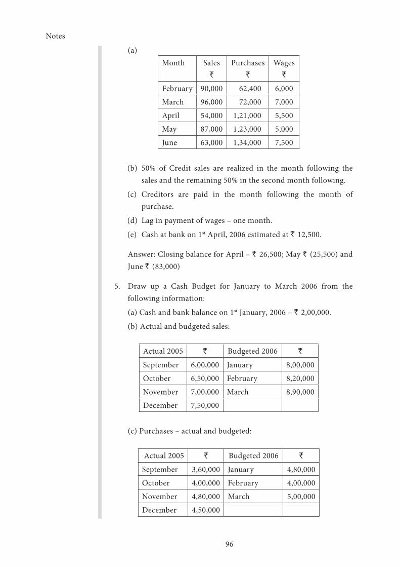
Notes

96

(a) Month Sales

`

Purchases`

Wages`

February 90,000 62,400 6,000

March 96,000 72,000 7,000

April 54,000 1,21,000 5,500

May 87,000 1,23,000 5,000

June 63,000 1,34,000 7,500

(b) 50% of Credit sales are realized in the month following the sales and the remaining 50% in the second month following.

(c) Creditors are paid in the month following the month of purchase.

(d) Lag in payment of wages – one month.

(e) Cash at bank on 1st April, 2006 estimated at ` 12,500.

Answer: Closing balance for April – ` 26,500; May ` (25,500) and June ` (83,000)

5. Draw up a Cash Budget for January to March 2006 from the following information:

(a) Cash and bank balance on 1st January, 2006 – ` 2,00,000.

(b) Actual and budgeted sales:

Actual 2005 ` Budgeted 2006 `

September 6,00,000 January 8,00,000

October 6,50,000 February 8,20,000

November 7,00,000 March 8,90,000

December 7,50,000

(c) Purchases – actual and budgeted:

Actual 2005 ` Budgeted 2006 `

September 3,60,000 January 4,80,000

October 4,00,000 February 4,00,000

November 4,80,000 March 5,00,000

December 4,50,000

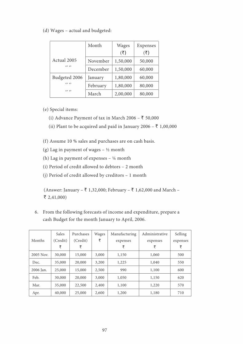
97

(d) Wages – actual and budgeted:

Actual 2005 ‘’ ‘’

Month Wages (`)

Expenses (`)

November 1,50,000 50,000

December 1,50,000 60,000

Budgeted 2006 ‘’ ‘’ ‘’ ‘’

January 1,80,000 60,000

February 1,80,000 80,000

March 2,00,000 80,000

(e) Special items:

(i) Advance Payment of tax in March 2006 – ` 50,000

(ii) Plant to be acquired and paid in January 2006 – ` 1,00,000

(f) Assume 10 % sales and purchases are on cash basis.

(g) Lag in payment of wages – ½ month

(h) Lag in payment of expenses – ¼ month

(i) Period of credit allowed to debtors – 2 month

(j) Period of credit allowed by creditors – 1 month

(Answer: January – ` 1,32,000; February – ` 1,62,000 and March – ` 2,41,000)

6. From the following forecasts of income and expenditure, prepare a cash Budget for the month January to April, 2006.

MonthsSales

(Credit)`

Purchases (Credit)

`

Wages`

Manufacturing expenses

`

Administrative expenses

`

Selling expenses

`

2005 Nov. 30,000 15,000 3,000 1,150 1,060 500

Dec. 35,000 20,000 3,200 1,225 1,040 550

2006 Jan. 25,000 15,000 2,500 990 1,100 600

Feb. 30,000 20,000 3,000 1,050 1,150 620

Mar. 35,000 22,500 2,400 1,100 1,220 570

Apr. 40,000 25,000 2,600 1,200 1,180 710

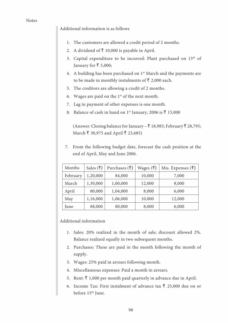
Notes

98

Additional information is as follows

1. The customers are allowed a credit period of 2 months.

2. A dividend of ` 10,000 is payable in April.

3. Capital expenditure to be incurred: Plant purchased on 15th of January for ` 5,000;

4. A building has been purchased on 1st March and the payments are to be made in monthly instalments of ` 2,000 each.

5. The creditors are allowing a credit of 2 months.

6. Wages are paid on the 1st of the next month.

7. Lag in payment of other expenses is one month.

8. Balance of cash in hand on 1st January, 2006 is ` 15,000

(Answer: Closing balance for January – ̀ 18,985; February ̀ 28,795; March ` 30,975 and April ` 23,685)

7. From the following budget date, forecast the cash position at the end of April, May and June 2006.

Months Sales (`) Purchases (`) Wages (`) Mis. Expenses (`)

February 1,20,000 84,000 10,000 7,000

March 1,30,000 1,00,000 12,000 8,000

April 80,000 1,04,000 8,000 6,000

May 1,16,000 1,06,000 10,000 12,000

June 88,000 80,000 8,000 6,000

Additional information

1. Sales: 20% realized in the month of sale; discount allowed 2%. Balance realized equally in two subsequent months.

2. Purchases: These are paid in the month following the month of supply.

3. Wages: 25% paid in arrears following month.

4. Miscellaneous expenses: Paid a month in arrears.

5. Rent: ` 1,000 per month paid quarterly in advance due in April.

6. Income Tax: First instalment of advance tax ` 25,000 due on or before 15th June.

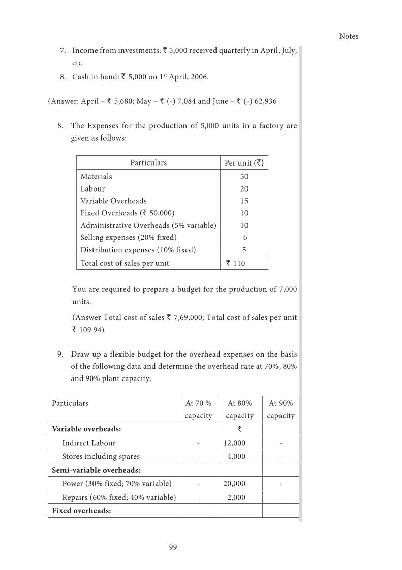
Notes

99

7. Income from investments: ` 5,000 received quarterly in April, July, etc.

8. Cash in hand: ` 5,000 on 1st April, 2006.

(Answer: April – ` 5,680; May – ` (-) 7,084 and June – ` (-) 62,936

8. The Expenses for the production of 5,000 units in a factory are given as follows:

Particulars Per unit (`)

Materials Labour Variable Overheads Fixed Overheads (` 50,000)Administrative Overheads (5% variable)Selling expenses (20% fixed)Distribution expenses (10% fixed)

5020151010 65

Total cost of sales per unit ` 110

You are required to prepare a budget for the production of 7,000 units.

(Answer Total cost of sales ` 7,69,000; Total cost of sales per unit ` 109.94)

9. Draw up a flexible budget for the overhead expenses on the basis of the following data and determine the overhead rate at 70%, 80% and 90% plant capacity.

Particulars At 70 % capacity

At 80% capacity

At 90% capacity

Variable overheads: `

Indirect Labour - 12,000 -

Stores including spares - 4,000 -

Semi-variable overheads:

Power (30% fixed; 70% variable) - 20,000 -

Repairs (60% fixed; 40% variable) - 2,000 -

Fixed overheads:

Notes

100

Depreciation - 11,000 -

Insurance - 3,000 -

Salaries - 10,000 -

Total Overheads - 62,000 -

Estimated direct labour hours - 124000 hrs -

(Answer: Overhead rate at 70% - ` 0.536; at 80% - ` 0.50 and at 90% - ` 0.472)

10. The cost of an article at a capacity level of 5,000 units is given under ‘A’ below. For a variation of 25% in capacity above or below this level, the individual expenses as indicated under ‘B’ below:

Cost per unit ` 12.55. Find out the cost per unit and total cost for production levels of 4,000 units and 6,000 units. Also show the total cost and unit cost for 5,000 units

Particulars ‘A’`

‘B”`

Material cost 25,000 (100% varying)

Labour cost 15,000 (100% varying)

Power 1,250 (80% varying)

Repairs and maintenance 2,000 (75% varying)

Stores 1,000 (100% varying)

Inspection 500 (20% varying)

Depreciation 10,000 (100% varying)

Administration overheads 5,000 (25% varying)

Selling overheads 3,000 (25% varying)

Total 62,750

(Answer: Total Cost at 4,000 units – ` 51,630; at 5,000 units – `

62,750 and at 6,000 units – ` 73,870. Cost per unit is ` 12.908; `

12.55 and ` 12.31 respectively.)

11. The expenses of budgeted production of 20,000 units in a factory are furnished below:

Notes

101

Particulars Per unit (`)

Materials 140

Labour 50

Variable overheads 40

Fixed overheads 20

Variable expenses (direct) 10

Selling expenses (10% fixed) 26

Distribution expenses (20% fixed) 14

Administrative expenses 10

Prepare a Flexible Budget for the production of 16,000 units and 12,000 units. Indicate cost per unit at both the levels.

(Answer: Cost per unit at 16,000 units – ` 318.85; at 12,000 units – ` 333.60)

12. Following is the data of a manufacturing concern. Calculate:-

Material Cost Variance, Material Price Variance and Material usage variance.

The standard quantity of materials required for producing one ton of output is 40 units. The standard price per unit of materials is `

3. During a particular period 90 tons of output was undertaken. The materials required for actual production were 4,000 units. An amount of ` 14,000 units. An amount of ` 14, 000 was spent on purchasing the materials.

(MCV: ` 3,200(A), MPV: ` 2,000 (A), MUV ` 1,200 (A)

13. The standard materials required for producing 100 units is 120 kgs. A standard price of 0.50 paise per kg is fixed 2,40,000 units were produced during the period. Actual materials purchased were 3,00,000 kgs. at a cost of ` 1,65,000. Calculate Materials Variance. ( MCV - 21,000)

14. From the data given below, calculate: Material Cost Variance, Material Price Variance and Material Usage Variance

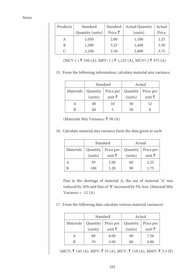
Notes

102

Products Standard Quantity (units)

Standard Price `

Actual Quantity (units)

Actual Price

ABC

1,0501,5002,100

2.003.253.50

1,1001,4002,000

2.253.503.75

(MCV (-) ` 550 (A), MPV: (-) ` 1,125 (A), MUV(-) ` 575 (A)

15. From the following information, calculate material mix variance:

Standard Actual

Materials Quantity (units)

Price per unit `

Quantity (units)

Price per unit `

AB

4060

105

5050

128

(Materials Mix Variance: ` 50 (A)

16. Calculate material mix variance form the data given as such:

Standard Actual

Materials Quantity (units)

Price per unit `

Quantity (units)

Price per unit `

AB

50100

2.001.20

6090

2.251.75

Due to the shortage of material A, the use of material ‘A’ was reduced by 10% and that of ‘B’ increased by 5% Ans: (Material Mix Variance = -12 (A)

17. From the following data calculate various material variances:

Standard Actual

Materials Quantity (units)

Price per unit `

Quantity (units)

Price per unit `

AB

8070

8.003.00

9080

7.504.00

(MCV; ` 145 (A), MPV: ` 35 (A), MUV: ` 110 (A), MMV: ` 3.3 (F)

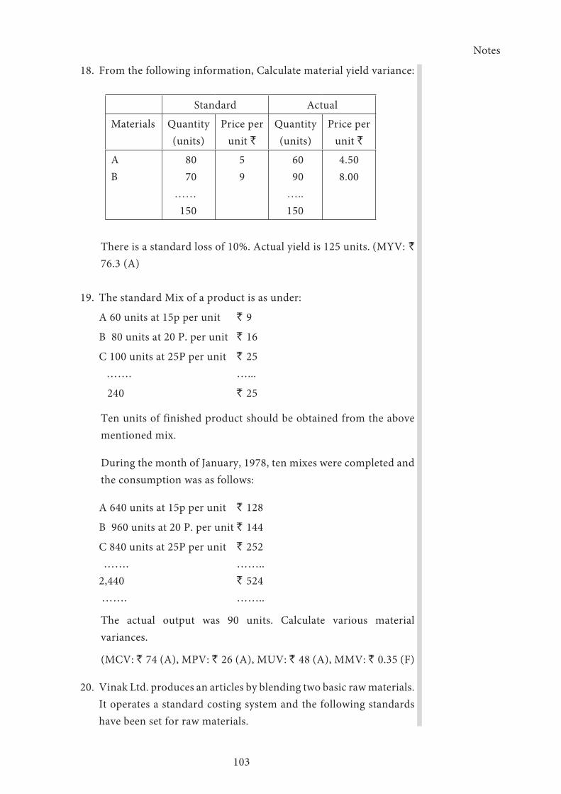
Notes

103

18. From the following information, Calculate material yield variance:

Standard Actual

Materials Quantity (units)

Price per unit `

Quantity (units)

Price per unit `

AB

8070

……150

59

6090

…..150

4.508.00

There is a standard loss of 10%. Actual yield is 125 units. (MYV: `

76.3 (A)

19. The standard Mix of a product is as under:

A 60 units at 15p per unit ` 9

B 80 units at 20 P. per unit ` 16

C 100 units at 25P per unit ` 25 ……. …...

240 ` 25

Ten units of finished product should be obtained from the above mentioned mix.

During the month of January, 1978, ten mixes were completed and the consumption was as follows:

A 640 units at 15p per unit ` 128

B 960 units at 20 P. per unit ` 144

C 840 units at 25P per unit ` 252 ……. ……..

2,440 ` 524 ……. ……..

The actual output was 90 units. Calculate various material variances.

(MCV: ` 74 (A), MPV: ` 26 (A), MUV: ` 48 (A), MMV: ` 0.35 (F)

20. Vinak Ltd. produces an articles by blending two basic raw materials. It operates a standard costing system and the following standards have been set for raw materials.

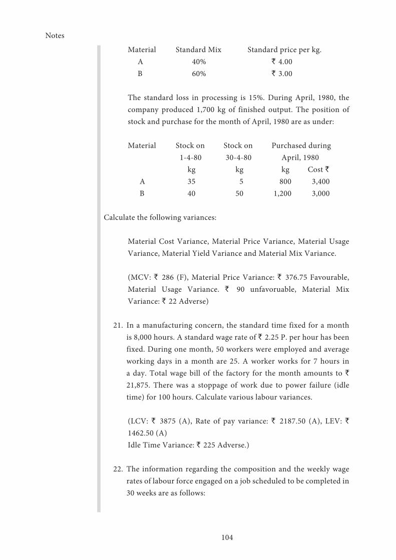
Notes

104

Material Standard Mix Standard price per kg. A 40% ` 4.00 B 60% ` 3.00

The standard loss in processing is 15%. During April, 1980, the company produced 1,700 kg of finished output. The position of stock and purchase for the month of April, 1980 are as under:

Material Stock on Stock on Purchased during 1-4-80 30-4-80 April, 1980 kg kg kg Cost `

A 35 5 800 3,400 B 40 50 1,200 3,000

Calculate the following variances:

Material Cost Variance, Material Price Variance, Material Usage Variance, Material Yield Variance and Material Mix Variance.

(MCV: ` 286 (F), Material Price Variance: ` 376.75 Favourable, Material Usage Variance. ` 90 unfavoruable, Material Mix Variance: ` 22 Adverse)

21. In a manufacturing concern, the standard time fixed for a month is 8,000 hours. A standard wage rate of ` 2.25 P. per hour has been fixed. During one month, 50 workers were employed and average working days in a month are 25. A worker works for 7 hours in a day. Total wage bill of the factory for the month amounts to `

21,875. There was a stoppage of work due to power failure (idle time) for 100 hours. Calculate various labour variances.

(LCV: ` 3875 (A), Rate of pay variance: ` 2187.50 (A), LEV: `

1462.50 (A) Idle Time Variance: ` 225 Adverse.)

22. The information regarding the composition and the weekly wage rates of labour force engaged on a job scheduled to be completed in 30 weeks are as follows:

Notes

105

Standard Actual

Category of wokers

No. of workers

Weekly wage rate per worker

No. of workers

Weekly wage rate per worker

SkilledSemi skilledUnskilled

754560

`

604020

703080

`

705020

The work was completed in 32 weeks. Calculate various labour variances.

23. The following data is taken out from the books of a manufacturing concern.

Budgeted labour composition for producing 100 articles

20 Men @ ` 1.25 hour for 25 hours

30 women @ 1.10 per hour for 30 hours

Actual labour composition for Producing 100 articles

25 Men @ ` 1.50 per hour for 24 hours

25 women @ ` 1.20 per hour for 25 hours

Calculate: (i) Labour Cost Variance, (ii) Labour Rate Variance, (iii) Labour Efficency Variance, (iv) Labour Mix Variance.

Ans:(Labour Cost Variance: ` 35 Adverse, Labour Rate Variacne ` 212.50 Adverse, LEV:` 177.50 Favourable and LMV: ` 24.38 unfavourable)

24. Calculate labour variances from the following data:

Standard ActualOut put in units 2,000 2,500

Number of workers employed 50 60

Number of working days in a month 20 22

Average wage per man per month (`) 280 330

Ans: LCV ` 2300 (A), LRV ` 1320 (A), LEV ` 980 (A)

Notes

106

25. From the following information compute;

(i) Fixed Overhead Variance

(ii) Expenditure Variance

(iii) Volume Variance

(iv) Capacity Variance

(v) Efficiency Variance

Budget Actual

Fixed overheads for November ` 20,000 20,400

Units of production in November 10,000 10,400

Standard time for 1 unit = 2 hours

Actual Hours Worked = 20,100 hours

Ans: Fixed Overhead Variance: ` 300 (A), Expenditure Variance: ` 400 (A), Volume Variance: ` 100 (F), Capacity Variance: ` 800 (F), Efficiency Variance: ` 700 (A)

26. From the following information, calculate various overhead variances:

Budget Actual

Output in units 12,000 14,000

Number of working days 20 22

Fixed Overheads 36,000 49,000

Variable Overheads 24,000 35,000

There was an increase of 5% in Capacity.

(Total Overhead cost Variance: `14,000 (A), Variable Overhead Variance: ` 7,000 (A), Fixed Overhead Variance: ` 7000 (A), Expenditure Variance: ` 13,000 (A), Volume Variance: ` 6000 (F), Capacity Variance: ` 1,800 (F), Calendar Variance: ` 32,780 (F), Efficiency Variance: ` 420 (F)

27. What is sales volume variance?

28. Briefly explain sales price variance

Notes

107

29. The budgeted and actual sales of a concern manufacturing and marketing a single product are furnished below:

Budgeted sales 10000 units at ` 4 per unit.

Actual sales 5000units at ` 3.5 per unit.

Calculate:

(i) Sales price variance

(ii) Sales volume variance

****

108

Notes

109

UNIT - III

Learning Objectives

On completion of this Unit you should be able to

➢ Understand the concepts of Marginal Costing, Absorption Costing or Full Cost Costing, Differential Costing, Marginal Cost, Fixed Cost, Variable Cost, Contribution, P / V ratio, Margin of Safety and Angle of Incidence.

➢ Explain CVP Analysis and know the construction of BEP chart

➢ List out the uses and limitations of BEP

➢ Know the role of marginal costing in decision making

➢ Explain managerial decisions which are taken with the help of marginal costing decisions in different situations.

Unit Structure

Lesson 3.1 - Marginal Costing – Basic Concepts

Lesson 3.2 - Marginal Costing and CVP Analysis

Lesson 3.3 - Marginal Costing and Decision-Making

Notes

110

Lesson 3.1 - Marginal Costing – Basic Concepts

Introduction

By analyzing the behavior of costs in relation to changes in volume of output it becomes evident that there are some items of costs which tend to vary directly with the volume of output. The cost that vary with volume of output, are called variable cost and those remain unaffected by change in volume of output are fixed cost or period costs.

Marginal costing is a study where the effect on profit of changes in the volume and type of output is analyzed. It is not a method of cost ascertainment like job costing or contract costing. It is a technique of costing oriented towards managerial decision making and control.

Marginal costing, being a technique can be used in combination with other technique such as budgeting and standard costing. It is helpful in determining the profitability of products, departments, processes, and cost centers. While analyzing the profitability, marginal costing interprets the cost on the basis of nature of cost. The emphasis is on behaviour of costs and their impact on profitability.

Definition

Marginal costing is defined by the ICWA, India as “the ascertainment of marginal costs and of the effect on profit of changes in volume or type of output by differentiating between fixed costs, and variable costs”

Batty defined Marginal Costing as, “a technique of cost accounting which pays special attention to the behaviour of costs with changes in the volume of output”

Kohler’s Dictionary for Accounting defines Marginal Costing “as the ascertainment of marginal or variable costs to an activity department or products as compared with absorption costing or direct costing”

Notes

111

The method of charging all the costs to production is called absorption costing. Kohler’s dictionary for Accountants defines it as “the process of allocating all or a portion of fixed and variable production costs to work – in – progress, cost of sales and inventory”. The net profits ascertained under this system will be different from that under marginal costing because of

➢ Difference in stock valuation

➢ Over and under – absorbed overheads

Direct costing is defined as the process of assigning costs as they are incurred to products and services

Features of Marginal Costing

The following are the special features of Marginal Costing:

➢ Marginal costing is a technique of working of costing which is used in conjunction with other methods of costing (Process or job)

➢ Fixed and variable costs are kept separate at every stage. Semi – Variable costs are also separated into fixed and variable.

➢ As fixed costs are period costs, they are excluded from product cost or cost of production or cost of sales. Only variable costs are considered as the cost of the product.

➢ As fixed cost is period cost, they are charged to profit and loss account during the period in which they incurred. They are not carried forward to the next year’s income.

➢ Marginal income or marginal contribution is known as the income or profit.

➢ The difference between the contribution and fixed costs is the net profit or loss.

➢ Fixed costs remains constant irrespective of the level of activity.

➢ Sales price and variable cost per unit remains the same.

➢ Cost volume profit relationship is fully employed to reveal the state of profitability at various levels of activity.

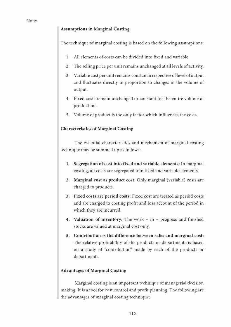
Notes

112

Assumptions in Marginal Costing

The technique of marginal costing is based on the following assumptions:

1. All elements of costs can be divided into fixed and variable.

2. The selling price per unit remains unchanged at all levels of activity.

3. Variable cost per unit remains constant irrespective of level of output and fluctuates directly in proportion to changes in the volume of output.

4. Fixed costs remain unchanged or constant for the entire volume of production.

5. Volume of product is the only factor which influences the costs.

Characteristics of Marginal Costing

The essential characteristics and mechanism of marginal costing technique may be summed up as follows:

1. Segregation of cost into fixed and variable elements: In marginal costing, all costs are segregated into fixed and variable elements.

2. Marginal cost as product cost: Only marginal (variable) costs are charged to products.

3. Fixed costs are period costs: Fixed cost are treated as period costs and are charged to costing profit and loss account of the period in which they are incurred.

4. Valuation of inventory: The work – in – progress and finished stocks are valued at marginal cost only.

5. Contribution is the difference between sales and marginal cost: The relative profitability of the products or departments is based on a study of “contribution” made by each of the products or departments.

Advantages of Marginal Costing

Marginal costing is an important technique of managerial decision making. It is a tool for cost control and profit planning. The following are the advantages of marginal costing technique:

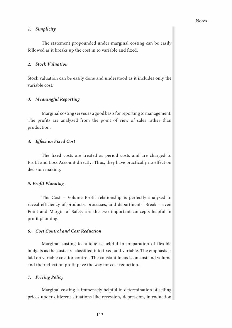
Notes

113

1. Simplicity

The statement propounded under marginal costing can be easily followed as it breaks up the cost in to variable and fixed.

2. Stock Valuation

Stock valuation can be easily done and understood as it includes only the variable cost.

3. Meaningful Reporting

Marginal costing serves as a good basis for reporting to management. The profits are analyzed from the point of view of sales rather than production.

4. Effect on Fixed Cost

The fixed costs are treated as period costs and are charged to Profit and Loss Account directly. Thus, they have practically no effect on decision making.

5. Profit Planning

The Cost – Volume Profit relationship is perfectly analysed to reveal efficiency of products, processes, and departments. Break – even Point and Margin of Safety are the two important concepts helpful in profit planning.

6. Cost Control and Cost Reduction

Marginal costing technique is helpful in preparation of flexible budgets as the costs are classified into fixed and variable. The emphasis is laid on variable cost for control. The constant focus is on cost and volume and their effect on profit pave the way for cost reduction.

7. Pricing Policy

Marginal costing is immensely helpful in determination of selling prices under different situations like recession, depression, introduction

Notes

114

of new product, etc. Correct pricing can be developed under the marginal costs technique with the help of the cost information revealed therein.

8. Helpful to Management

Marginal costing is helpful to the management in exercising decisions regarding make or buy, exporting, key factor and numerous other aspects of business operations.

Limitations of Marginal Costing

Following are the limitations of marginal costing:

• ClassificationofCost

Break up of cost into fixed and variable portion is a difficult problem. More over clear cost division of semi – variable or semi – fixed cost is complicated and cannot be accurate.

• NotSuitableforExternalReporting

Since fixed cost is not included in total cost, full cost is not available to outsiders to judge the efficiency.

• LackofLong–termPerspective

Marginal costing is most suitable for decision making in a short term. It assumes that costs are classified into fixed and variable. In the long term all the cost are variable. Therefore it ignores time element and is not suitable for long term decisions.

• UnderValuationofStock

Under marginal costing only variable costs are considered and the output as well as stock are undervalued and profit is distorted. When there is loss of stock the insurance cover will not meet the total cost.

• Automation

In these days of automation and technical advancement, huge investments are made in heavy machinery which results in heavy amount of fixed costs. Ignoring fixed cost in this context for decision making is irrational.

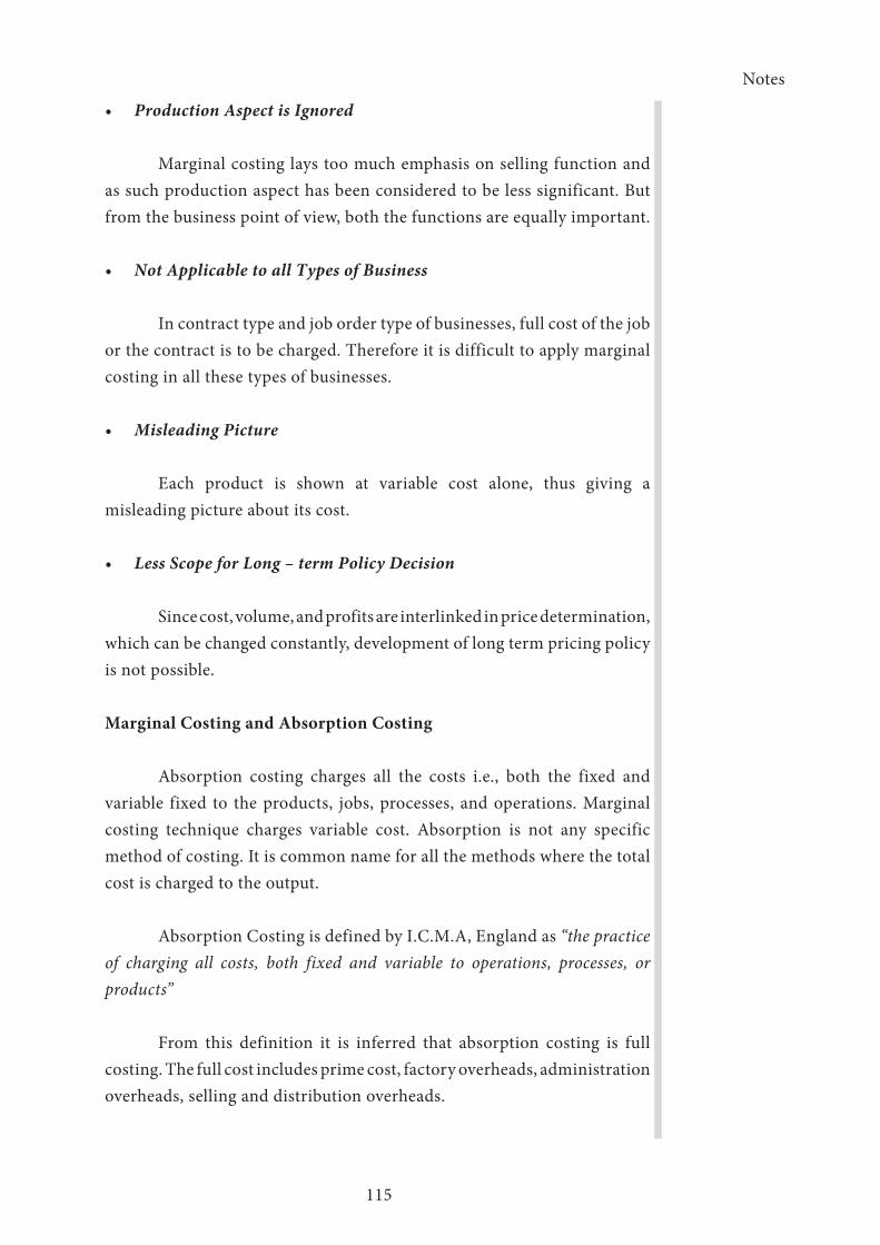
Notes

115

• ProductionAspectisIgnored

Marginal costing lays too much emphasis on selling function and as such production aspect has been considered to be less significant. But from the business point of view, both the functions are equally important.

• NotApplicabletoallTypesofBusiness

In contract type and job order type of businesses, full cost of the job or the contract is to be charged. Therefore it is difficult to apply marginal costing in all these types of businesses.

• MisleadingPicture

Each product is shown at variable cost alone, thus giving a misleading picture about its cost.

• LessScopeforLong–termPolicyDecision

Since cost, volume, and profits are interlinked in price determination, which can be changed constantly, development of long term pricing policy is not possible.

Marginal Costing and Absorption Costing

Absorption costing charges all the costs i.e., both the fixed and variable fixed to the products, jobs, processes, and operations. Marginal costing technique charges variable cost. Absorption is not any specific method of costing. It is common name for all the methods where the total cost is charged to the output.

Absorption Costing is defined by I.C.M.A, England as “the practice of charging all costs, both fixed and variable to operations, processes, or products”

From this definition it is inferred that absorption costing is full costing. The full cost includes prime cost, factory overheads, administration overheads, selling and distribution overheads.

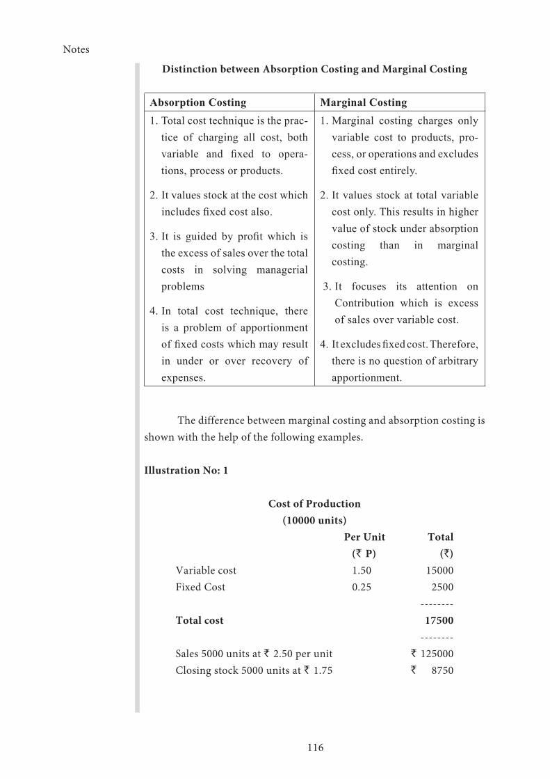
Notes

116

Distinction between Absorption Costing and Marginal Costing

Absorption Costing Marginal Costing1. Total cost technique is the prac-

tice of charging all cost, both variable and fixed to opera-tions, process or products.

2. It values stock at the cost which includes fixed cost also.

3. It is guided by profit which is the excess of sales over the total costs in solving managerial problems

4. In total cost technique, there is a problem of apportionment of fixed costs which may result in under or over recovery of expenses.

1. Marginal costing charges only variable cost to products, pro-cess, or operations and excludes fixed cost entirely.

2. It values stock at total variable cost only. This results in higher value of stock under absorption costing than in marginal costing.

3. It focuses its attention on Contribution which is excess of sales over variable cost.

4. It excludes fixed cost. Therefore, there is no question of arbitrary apportionment.

The difference between marginal costing and absorption costing is shown with the help of the following examples.

Illustration No: 1

Cost of Production(10000 units)

Per Unit Total (` P) (`)Variable cost 1.50 15000Fixed Cost 0.25 2500

--------Total cost 17500

--------Sales 5000 units at ` 2.50 per unit ` 125000Closing stock 5000 units at ` 1.75 ` 8750

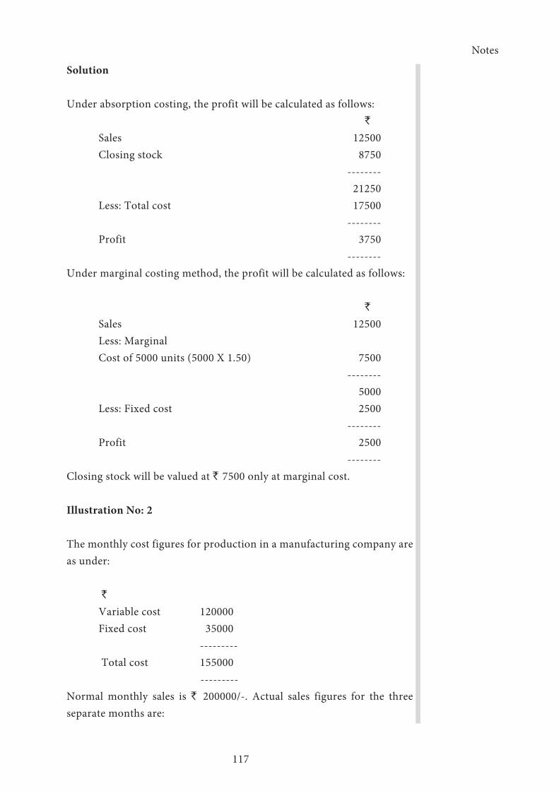
Notes

117

Solution

Under absorption costing, the profit will be calculated as follows: `

Sales 12500Closing stock 8750 -------- 21250Less: Total cost 17500 --------Profit 3750 --------

Under marginal costing method, the profit will be calculated as follows:

`

Sales 12500Less: MarginalCost of 5000 units (5000 X 1.50) 7500 -------- 5000Less: Fixed cost 2500 --------Profit 2500 --------

Closing stock will be valued at ` 7500 only at marginal cost.

Illustration No: 2

The monthly cost figures for production in a manufacturing company are as under:

`

Variable cost 120000Fixed cost 35000 --------- Total cost 155000

---------Normal monthly sales is ` 200000/-. Actual sales figures for the three separate months are:

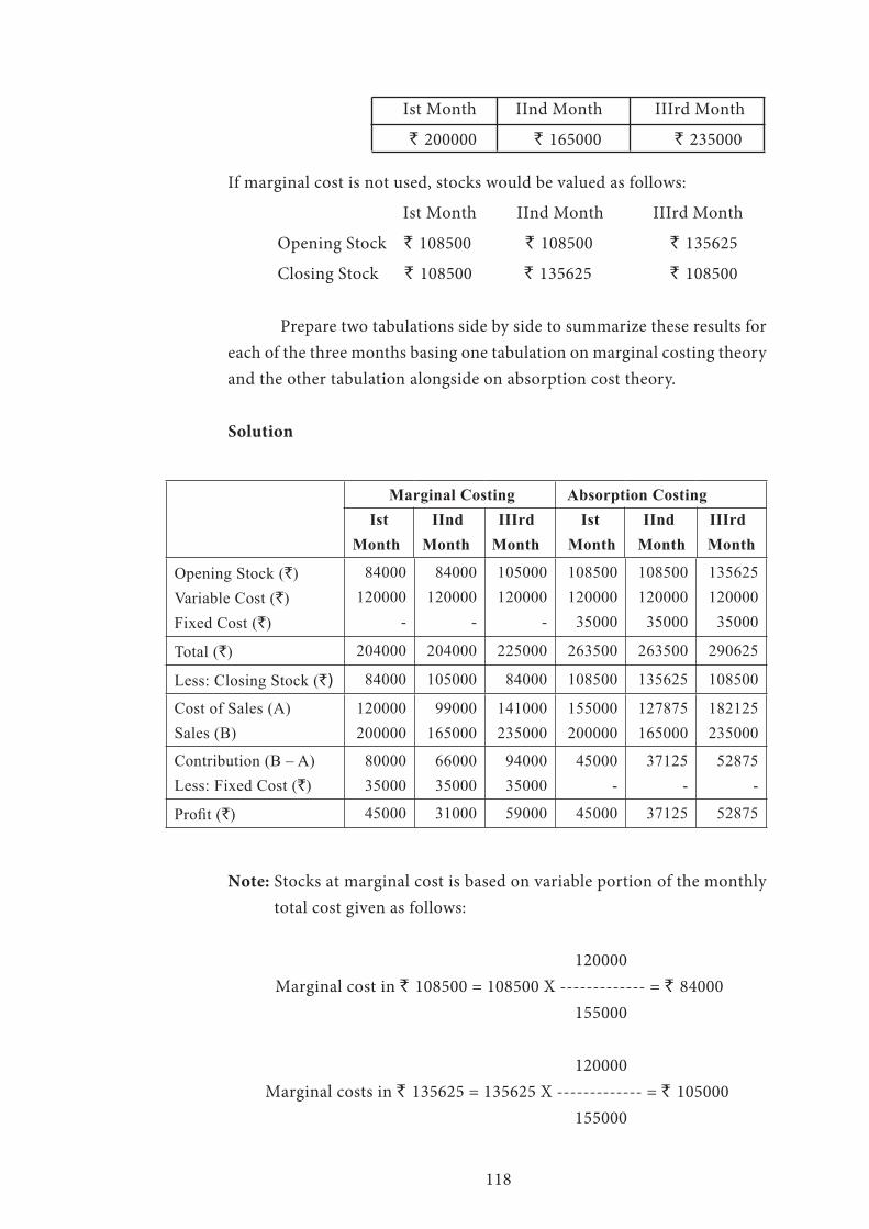
118

Ist Month IInd Month IIIrd Month

` 200000 ` 165000 ` 235000

If marginal cost is not used, stocks would be valued as follows:

Ist Month IInd Month IIIrd Month

Opening Stock ` 108500 ` 108500 ` 135625

Closing Stock ` 108500 ` 135625 ` 108500

Prepare two tabulations side by side to summarize these results for each of the three months basing one tabulation on marginal costing theory and the other tabulation alongside on absorption cost theory.

Solution

Marginal Costing Ist IInd IIIrdMonth Month Month

Absorption Costing Ist IInd IIIrd Month Month Month

Opening Stock (`)Variable Cost (`)Fixed Cost (`)

84000120000

-

84000120000

-

105000120000

-

108500120000 35000

108500120000 35000

135625120000 35000

Total (`) 204000 204000 225000 263500 263500 290625

Less: Closing Stock (`) 84000 105000 84000 108500 135625 108500

Cost of Sales (A)Sales (B)

120000200000

99000165000

141000235000

155000200000

127875165000

182125235000

Contribution (B – A)Less: Fixed Cost (`)

80000 35000

66000 35000

94000 35000

45000 -

37125 -

52875 -

Profit (`) 45000 31000 59000 45000 37125 52875

Note: Stocks at marginal cost is based on variable portion of the monthly total cost given as follows:

120000 Marginal cost in ` 108500 = 108500 X ------------- = ` 84000

155000

120000Marginal costs in ` 135625 = 135625 X ------------- = ` 105000

155000

Notes

119

Differential Costing

The concept of differential cost is a relevant cost concept in those decision situations which involve alternative choices. It is the difference in the total costs of two alternatives. This helps in decision making. It can be determined by subtracting the cost of one alternative from the cost of another alternative. Differential costing is the change in the total cost which results from the adoption of an alternative course of action. The alternative may arise on account of sales, volume, price change in sales mix, etc decisions. Differential cost analysis leads to more correct decisions than more marginal costing analysis. In this technique the total costs are considered and not the cost per unit. Differential costs do not form part of the accounting system while marginal costing can be adapted to the routine accounting itself. However, when decisions involve huge amount of money differential cost analysis proves to be useful.

In the illustration given below, differential cost at levels of activity has been shown:

Alternative I Alternative II Differential cost

Activity level Sales (`) 80% 100%

80000 100000 20000----------------------------------------------------

Direct materials 40000 50000 10000Direct labour 16000 20000 4000Variable overheads 4000 5000 1000Fixed overheads 3000 3000 -

-----------------------------------------------------Cost of sales 63000 78000 15000 -----------------------------------------------------

Differential cost is generally confused with marginal cost. Of course, these two techniques are similar in some aspects but these also differ in certain other respects.

Similarities

(i) Both the differential cost analysis and marginal cost analysis are based on the classification of cost into fixed and variable. When

Notes

120

fixed costs do not change, both differential and marginal costs are same.

(ii) Both are the techniques of cost analysis and presentation and are used by the management in formulating policies and decision making.

Dissimilarities

(i) Marginal cost may be incorporated in the accounting system where as differential cost are worked out for reporting to the management for taking certain decisions.

(ii) Entire fixed cost are excluded from costing where as some of the relevant fixed costs may be included in the differential cost analysis.

(iii) In marginal costing, contribution and p/v ratio are the main yard-stick for evaluating performance and decision making. In differ-ential cost analysis emphasis is made between differential cost and incremental or decremental revenue for making policy decisions.

(iv) Differential cost analysis may be used in absorption costing and marginal costing.

Marginal Cost

Marginal cost is the cost of producing one additional unit of output. It is the amount by which total cost increases when one extra unit is produced or the amount of cost which can be avoided by producing one unit less.

The ICMA, England defines marginal cost as, “the amount of any given volume of output by which the aggregate cost are charged if the volume of output is increased or decreased by one unit”.

In practice, this is measured by the total cost attributable to one unit. In this context, a unit may be single article, a batch of articles, an order, a stage of production, a process etc., often managerial costs, variable costs are used to mean the same.

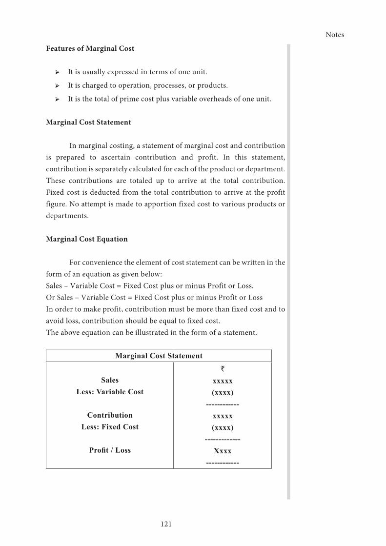
Notes

121

Features of Marginal Cost

➢ It is usually expressed in terms of one unit.

➢ It is charged to operation, processes, or products.

➢ It is the total of prime cost plus variable overheads of one unit.

Marginal Cost Statement

In marginal costing, a statement of marginal cost and contribution is prepared to ascertain contribution and profit. In this statement, contribution is separately calculated for each of the product or department. These contributions are totaled up to arrive at the total contribution. Fixed cost is deducted from the total contribution to arrive at the profit figure. No attempt is made to apportion fixed cost to various products or departments.

Marginal Cost Equation

For convenience the element of cost statement can be written in the form of an equation as given below:Sales – Variable Cost = Fixed Cost plus or minus Profit or Loss.Or Sales – Variable Cost = Fixed Cost plus or minus Profit or LossIn order to make profit, contribution must be more than fixed cost and to avoid loss, contribution should be equal to fixed cost. The above equation can be illustrated in the form of a statement.

Marginal Cost Statement

SalesLess: Variable Cost

ContributionLess: Fixed Cost

Profit / Loss

`

xxxxx(xxxx)

------------xxxxx(xxxx)

-------------Xxxx

------------

Notes

122

Illustration No.3

A company is manufacturing three products X, Y and Z. It supplies you the following information:

Products ------------------------------------ X Y Z (`) (`) (`)Direct Materials 2500 10000 1000Direct Labour 3000 3000 500 Variable Overheads 2000 5000 2500Sales 10000 20000 5000

Total fixed overheads ` 3000/-Prepare a marginal cost statement and determine profit and loss.

Solution

Marginal Cost Statement

Products----------------------------------------------- X Y Z Total (`) (`) (`) (`)

Sales (A) 10000 20000 5000 35000 -----------------------------------------------Direct materials 2500 10000 1000 13500Direct Labour 3000 3000 500 6500Variable Overheads 2000 5000 2500 9500 -----------------------------------------------Marginal Cost (B) 7500 18000 4000 29500 -----------------------------------------------Marginal Contribution (A – B) 2500 2000 1000 5500Less: Fixed Cost 3000 ------- Net Profit 2500

Notes

123

Contribution

Contribution is the difference between selling price and variable cost of one unit. The greater contribution from the selling unit indicates that the variable cost is less compared to selling price. Total contribution is the number of units multiplied by contribution per unit. Contribution will be equal to the total fixed costs at break even point where profit is zero.

Illustration No.4

Calculate contribution and profit from the following details:

Sales ` 12000

Variable Cost ` 7000

Fixed Cost ` 4000

Solution:

Contribution = Sales – Variable cost

Contribution = ` 12000 – ` 7000 = ` 5000

Profit = Contribution – Fixed Cost

Profit = ` 5000 – ` 4000 = ` 1000

Profit / Volume Ratio

This is the ratio of contribution to sales. It is an important ratio analysing the relationship between sales and contribution. A high p/v ratio indicates high profitability and low p/v ratio indicates low profitability. This ratio helps in comparison of profitability of various products. Since high p/v ratio indicates high profits, the objective of every organisation should be to improve or increase the p/v ratio.

P / V Ratio = Contribution / Sales x 100 or C / S x 100(Or)

Fixed Cost + Profit-----------------------

Sales(Or)

Sales – Variable Cost-------------------------

Sales

Notes

124

When profits and sales for two consecutive periods are given, the following formula can be applied:

Change in Profit --------------------

Change in Sales

P / V ratio is also used in making the following type of calculations:

a) Calculation of Break even point.

b) Calculation of profit at a given level of sales.

c) Calculation of the volume of sales required to earn a given profit.

d) Calculation of profit when margin of safety (discussed below) is given.

e) Calculation of the volume of sales required to maintain the present level of profit if selling price is reduced.

Margin of Safety

The excess of actual or budgeted sales over the break-even sales is known as the margin of safety.

Margin of safety = actual sales - break-even sales

So this shows the sales volume which gives profit. Larger the margin of safety greater is the profit.

Budget sales - break-even salesMargin of safety ratio = -----------------------------------

Budget sales

(Or)

Profit----------P/V Ratio

When margin of safety is not satisfactory, the following corrective steps may be undertaken:

Notes

125

a) Increase the volume of sales.

b) Increase the selling price.

c) Reduce fixed cost.

d) Reduce variable cost.

e) Improve sales mix by increasing the sale of products with P/V ratio.

The effect of a price reduction will always reduce the P / V ratio, raise the break – even point, shorten the margin of safety.

Angle of Incidence

1. This is obtained from the graphical representation of sales and cost. When sales and output in units are plotted against cost and revenue, the angle formed between the total sales line and the total cost line at the break-even point is called the angle of incidence.

Large angle indicates a high rate of profit while a narrow angle would refer to a relatively low rate of profit.

Profit Goal

To earn a desired amount of profit i.e., a profit goal can be reached by the formula given below

Fixed cost + Desired profitability

Sales volume to reach profit goal = ------------------------------------------ Contribution ratio

If the profit goal is stated in terms of profit after taxes

Fixed cost + {(desired after-tax profit)/1-tax rate}

Sales volume to reach profit goal = ------------------------------------------ Contribution ratio

Operating leverage: An important concept in context of the CVP analysis is the operating leverage. This refers to the use of the fixed costs in the operation of a firm, and it accentuates fluctuations in the firm’s

Notes

126

operating profit due to change in sales. Thus the degree of operating leverage may be defined as the percentage change in operating profit (earning before interest and tax) on account of a change in sales.

% Change in operating profitDegree of Leverage DOL= --------------------------------------

% Change in sales

(Or)

Change in EBIT ------------------

EBITDegree of Leverage DOL= ------------------ Change in sales

------------ Sales

****

Notes

127

Lesson 3.2 - Marginal Costing and CVP Analysis

Introduction

Break-even analysis is the form of CVP analysis. It indicates the level of sales at which revenues equal costs. This equilibrium point is called the breakeven point. It is the level of activity where total revenue equals total cost. It is alternatively called as CVP analysis also. But it is said that the study up to the state of equilibrium is called as break even analysis and beyond that point we term it as CVP analysis.

Cost – Volume Profit analysis helps the management in profit planning. Profits are affected by several internal and external factors which influence sales revenues and costs.

The objectives of cost-volume profit analysis are:

i) To forecast profits accurately.

ii) To help to set up flexible budgets.

iii) To help in performance evaluation for purposes of control.

iv) To formulate proper pricing policy.

v) To know the overheads to be charged to production at various levels.

Volume or activity can be expressed in any one of the following ways:

1. Sales capacity expressed as a percentage of maximum sales.

2. Sales value in terms of money.

3. Units sold.

4. Production capacity expressed in percentages.

5. Value of cost of production.

6. Direct labour hours.

7. Direct labour value.

8. Machine hours.

Notes

128

The factors which are usually involved in this analysis are:

a) Selling price

b) Sales volume

c) Sales mix

d) Variable cost per unit

d) Total fixed cost

Break Even Chart

The chart depicts the interplay of three elements viz., cost, volume, and profits. The chart is a graph which at a glance provide information of fixed costs, variable costs, production / sales achieved profits etc., and also the trends in each one of them. The conventional graph is as follows:

This is a simple break even chart. The procedure for drawing the chart is as follows:

1) Take X - axis as the volume of sales or capacity or production.

2) Take Y – axis as the costs or revenue.

3) Having known at ‘0’ level of activity the same fixed cost is incurred, the fixed cost line drawn parallel to the X – axis.

4) At ‘0’ level of activity, the total cost is equal to fixed cost. Therefore the total cost line starts from the point where the fixed cost line meets the Y – axis.

Notes

129

5) Next plot the sales line starting from ‘0 ’.

6) The meeting point of the sales and the total cost line is the Break Even Point.

It is also called Break Even Point because at this point there is no profit and loss either.

The costs are just recovery by sales. If a perpendicular line is drawn to the X- axis from the BEP, the meeting point of the perpendicular and X- axis will show the break even volume in units. If a perpendicular line is drawn to meet the Y- axis from the BEP, the meeting point shows the break even volume in money terms.

Other details shown in the break even charts are:

Angle of Incidence

This is the angle of intersection between the sales line and the total cost line. The larger the angle the greater is the profit or loss, as the case may be.

Margin of Safety

This is the difference between the actual sales level and the break even sales. It represents the “cushion” for the company. The larger the distance between the break even sales volume and the actual sales volume, more comfortably the company can afford to allow the fall in sales without the danger of incurring losses. If the margin of safety is low i.e., if the distance between the actual sales line and the break even sales line is too short, even a small fall in the sales volume will drive the company into the loss area.

The position of breakeven point should be ideally closer to the y – axis. This will mean that even a small increase in sales will immediately make the company break even. I t should be noted that beyond the breakeven point all contribution (Sales – Marginal Cost) will directly add the profits.

Notes

130

Profit Volume Graph

Profit volume graph is a pictorial representation of the profit volume relationship. It shows profit and loss account at different volumes of sales. It is simplified form of break even chart as it clearly represents the relationship of profit to volume of sales. It is possible to construct a profit volume graph for any data relating to a business firm where a break even chart can be drawn. A profit volume graph may be preferred to a break even chart as profit or losses can be directly read at different levels of activity.

The construction of profit volume graph involves the following steps:

1. Scale of sale is selected on horizontal axis (i.e. ‘X’ axis) and that for profit or loss are selected on vertical axis (i.e. ‘Y’ axis). The area below the horizontal axis is the loss area and that above it is the profit area.

2. Points of profits of corresponding sales are plotted and joined. The resultant line is profit / loss line

Illustration No. 1

Draw up a profit – volume of the following:Sales ` 4 LakhsVariable cost ` 2 LakhsFixed cost ` 1 LakhsProfit ` 1 Lakhs

Notes

131

Solution

The calculation of BEP is based on some assumptions. They are as follows:

1. The costs are classified as fixed and variable costs.

2. The variable costs vary with volume and the fixed costs remain constant.

3. The selling price remains constant in spite of the change in volume.

4. The productivity per employee also remains unchanged.

Break-even point can be calculated in terms of units or in terms of rupees.

Fixed CostsBreak-Even Point (in Rupees) = -------------

P/V Ratio

(OR)

Fixed CostsBreak-Even Point (in Rupees) = ---------------------------------------------

Marginal cost per unit/1- Selling price per unit

Fixed CostsBreak-Even Point (in units) = ------------------------ Contribution per unit

Where contribution is sales - variable cost and P/V Ratio is Contribution divided by sales.

Cost-volume-profit relationship with the help of an example

The relationship between cost volume and profit are well defined in CVP analysis. With the given example we can elaborately see the relationship

AB Company is a single product manufacturer whose selling price is ` 20 per unit and the variable cost is ` 12 per unit. The annual fixed cost is ` 160000. The number of units produced and sold is 20000. Now if we analyse the CVP relationship

Notes

132

The contribution per unit is = Selling price -variable cost = 20 - 12 = ` 8/-

The total contribution for 20000 units is = 8 x 20000 = 160000

Since the profit = total contribution - fixed cost, we get nil profit. 160000-160000=0

This is the break even point where the total cost is equal to the total revenue and the company has no profit and no loss.

Let us see a few alternatives

If the fixed cost is ` 120000, then the company may earn a profit of ` (160000-120000) = 40000. If the fixed cost is ` 200000, then it may end in a loss of Rs (200000-160000) = 40000

If the variable cost per unit is increased, say to ` 15 in the existing condition, then the contribution will come to Rs (20000 x (20-15) = 100000 and that will result in a loss of ` 160000-100000 =40000. If the variable cost per unit is decreased say to ` 10 then the contribution will come to ` 20000x (20-10) = 200000. Then the profit will be 200000-160000=40000

The above proves that the variation in the costs changes the profitability of the firm.

If the cost decreases, profit increases and vice versa.

Now we can see how the change in volume alters the profitability. If the sales volume is 10000 instead of 20000 as above and the all the other conditions being the same, the result will be (10000x8) - 160000 = 80000 loss. Likewise if the volume is increased to 30000 it will result in a profit of ` 30000x8 - 160000 = 80000. This shows that the profit increases with the increase in volume when other conditions are unchanged.

Basic Assumptions of Cost – Volume Profit Analysis

Cost volume profit (C-V-P) analysis, popularly referred to as breakeven analysis, helps in answering questions like: How do costs behave

Notes

133

in relation to volume? At what sales volume would the firm breakeven? How sensitive is profit to variations in output? What would be the effect of a projected sales volume on profit? How much should the firm produce and sell in order to reach a target profit level?

A simple tool for profit planning and analysis, cost-volume-profit analysis is based on several assumptions. Effective use of this analysis calls for an understanding of the significance of these assumptions which are discussed below:

i. The behaviour of costs is predictable. The conventional cost-volume-profit model is based on the assumption that the cost of the firm is divisible into two components; fixed costs vary variable costs. Fixed costs remain unchanged for all ranges of output; variable costs vary proportionately to volume. Hence the behaviour of costs is predictable. In reality, however, it is not necessary for these assumptions to be valid over the entire range of volume. If they are valid over the range of output within which the firm is most likely to operate – referred to as the relevant range – cost volume profit analysis is a useful tool.

ii. The unit selling price is constant. This implies that the total revenue of the firm is a linear function of output. For firms which have a strong market for their products, this assumption is quite valid. For other firms, however, it may not be so. Price reduction might be necessary to achieve a higher level of sales. On the whole, however, this is a reasonable assumption and not unrealistic enough to impair the validity of the cost-volume- profit model, particularly in the relevant range of output.

iii. The firm manufactures a stable product – mix. In the case of a multi-product firm, the cost volume profit model assumes that the product – mix of the firm remains stable. Without this premise it is not possible to define the average variable profit ratio when different products have different variable profit ratios. While it is necessary to make this assumption, it must be borne in mind that the actual mix of products may differ from the planned one. Where this discrepancy is likely to be significant, cost-volume-profit model has limited applicability.

Notes

134

iv. Inventory changes are nil. A final assumption underlying the conventional cost-volume-profit model is that the volume of sales is equal to the volume of production during an accounting period. Put differently, inventory changes are assumed to be nil. This is required because in cost-volume-profit analysis we match total costs and total revenues for a particular period.

Uses and Limitations of Break Even Analysis

Uses of BE analysis are as follows:

1. It is a simple device and easy to understand.

2. It is of utmost use in profit planning.

3. It provides the basic information for further profit improvement studies.

4. It is useful in decision making and it helps in considering the risk implications of alternative actions.

5. It helps in finding out the effect of changes in the price, volume, or cost.

6. It helps in make or buys decisions also and helpful in the critical circumstances to find out the minimum profitability the firm can maintain.

The Limitations of BE Analysis is

1. The basis assumptions are at times base less. For example, we can say that the fixed costs cannot remain unchanged all the time. And the constant selling price and unit variable cost concept are also not acceptable.

2. It is difficult to segregate the cost components as fixed and variable costs.

3. It is difficult to apply for multinational companies.

4. It is a short-run concept and has a limited use in long range planning.

5. It is a static tool since it gives the relationship between cost, volume and profit at a given point of time and

6. It fails to predict future revenues and costs.

Notes

135

Despite the limitation it remains an important tool in profit planning due to the simplicity in calculation.

Illustration No. 2

From the following data calculate

(a) P/V Ratio (b) Variable Cost and (c) Profit `

Sales 80000Fixed expenses 15000Breakeven point 50000

Solution

Calculation of P/V Ratio

Breakeven point =Fixed Cost / P/V Ratio

50000 = 15000 / P/V Ratio = 15,000 / 50,000 = 3/10 or 30%

Calculation of variable cost

Contribution = Sales x P/V = 80,000 x 30 / 100 = ` 24000

Variable cost = Sales – Contribution ` 80000 – ` 24000 = ` 56000

Calculation of Profit

Profit = Contribution – Fixed cost = ` 24000 – ` 15000 = ` 9000

Illustration No. 3

From the following data, calculate the break-even point of sales in rupees:

Selling priceVariable cost per unit:ManufacturingSellingOverhead (fixed):Factory overheadsSelling overheads

`

20

105

500000200000

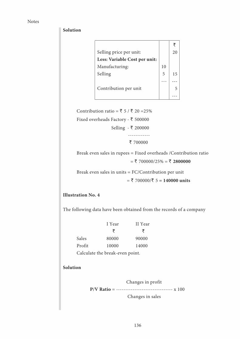
Notes

136

Solution

Selling price per unit:Less: Variable Cost per unit:Manufacturing:Selling

Contribution per unit

10 5 ---

`

20

15---

5---

Contribution ratio = ` 5 / ` 20 =25%

Fixed overheads Factory - ` 500000

Selling - ` 200000 ------------ ` 700000

Break even sales in rupees = Fixed overheads /Contribution ratio

= ` 700000/25% = ` 2800000

Break even sales in units = FC/Contribution per unit

= ` 700000/` 5 = 140000 units

Illustration No. 4

The following data have been obtained from the records of a company

I Year II Year ` `

Sales 80000 90000Profit 10000 14000Calculate the break-even point.

Solution

Changes in profit P/V Ratio = ------------------------------- x 100

Changes in sales

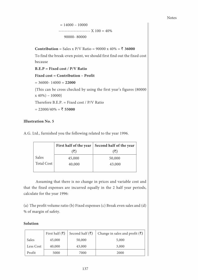
Notes

137

= 14000 – 10000 --------------------- X 100 = 40%

90000- 80000

Contribution = Sales x P/V Ratio = 90000 x 40% = ` 36000

To find the break-even point, we should first find out the fixed cost because

B.E.P = Fixed cost / P/V Ratio

Fixed cost = Contribution – Profit

= 36000- 14000 = 22000

{This can be cross checked by using the first year’s figures (80000 x 40%) – 10000}

Therefore B.E.P. = Fixed cost / P/V Ratio

= 22000/40% = ` 55000

Illustration No. 5

A.G. Ltd., furnished you the following related to the year 1996.

SalesTotal Cost

First half of the year (`)

Second half of the year (`)

45,000 40,000

50,000 43,000

Assuming that there is no change in prices and variable cost and that the fixed expenses are incurred equally in the 2 half year periods, calculate for the year 1996:

(a) The profit volume ratio (b) Fixed expenses (c) Break even sales and (d) % of margin of safety.

Solution

First half (`) Second half (`) Change in sales and profit (`)

Sales 45,000 50,000 5,000

Less Cost 40,000 43,000 3,000

Profit 5000 7000 2000

Notes

138

a) P/V ratio=Change in profit / Change in sales x 100

= 2000 / 5000 x 100 = 40%.

Contribution during the first half=Sales x P/V Ratio

= ` 45000 x 40% = ` 18000

b) Fixed cost = Contribution – ProfitFor1sthalfyear=18,000 – 5,000 = ` 13,000

Fixed cost for the full year =13,000 x 2 = ` 26000

c) Break even sales=Fixed cost / P/V Ratio for the year1996=26000 / 40% = ` 65000

d) Margin of safety=Sales – Break even sales for the year1996 (MOS) = 95000 – 65000 = ` 30000

Percent of margin of safety = Margin of safety / Sales for the year x 100

= 30000 / 95000 x 100

Note: (1) Since fixed expenses are incurred equally in the 2 half years, ` 13000 is multiplied with 2 to get fixed cost of the full year.

(2) Sales of both 1st and 2nd half years are added and are taken as actual sales i.e., ` 95000 to calculated margin of safety.

Illustration No.6

From the following information relating to Palani Bros. Ltd., you are required to find out: (a) P/V Ratio (b) Break even point (c) Profit (d) Margin of safety (e) Volume of sales to earn profit of ` 6000.

Total Fixed CostTotal variable costTotal Sales

`

45007500

15000

Notes

139

Solution

SalesLess: Variablecost

ContributionLess: Fixed cost

Profit

Amount(`)

150007500

-------- 7500

4500--------

3000--------

(a) P/V ratio =Contribution / Sales x 100

= 7500 / 15000 x 100 = 50%

(b) Break even sales = Fixed expenses / P/V Ratio= 4500+ 6000 / 50% = ` 21000

Illustration No. 7

The sales turnover and profit during two years were as follows:

Year Sales (`)

Profit(`)

19911992

140000160000

1500020000

Calculate

(a) P/V Ratio

(b) Break-even point

(c) Sales required to earn a profit of ` 40000

(d) Fixed expenses and

(e) Profit when sales are ` 120000

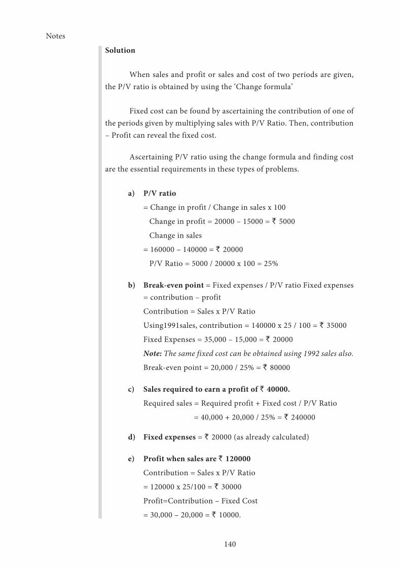
Notes

140

Solution

When sales and profit or sales and cost of two periods are given, the P/V ratio is obtained by using the ‘Change formula’

Fixed cost can be found by ascertaining the contribution of one of the periods given by multiplying sales with P/V Ratio. Then, contribution – Profit can reveal the fixed cost.

Ascertaining P/V ratio using the change formula and finding cost are the essential requirements in these types of problems.

a) P/V ratio

= Change in profit / Change in sales x 100

Change in profit = 20000 – 15000 = ` 5000

Change in sales

= 160000 – 140000 = ` 20000

P/V Ratio = 5000 / 20000 x 100 = 25%

b) Break-even point = Fixed expenses / P/V ratio Fixed expenses = contribution – profit

Contribution = Sales x P/V Ratio

Using1991sales, contribution = 140000 x 25 / 100 = ` 35000

Fixed Expenses = 35,000 – 15,000 = ` 20000

Note: The same fixed cost can be obtained using 1992 sales also.

Break-even point = 20,000 / 25% = ` 80000

c) Sales required to earn a profit of ` 40000.

Required sales = Required profit + Fixed cost / P/V Ratio

= 40,000 + 20,000 / 25% = ` 240000

d) Fixed expenses = ` 20000 (as already calculated)

e) Profit when sales are ` 120000

Contribution = Sales x P/V Ratio

= 120000 x 25/100 = ` 30000

Profit=Contribution – Fixed Cost

= 30,000 – 20,000 = ` 10000.

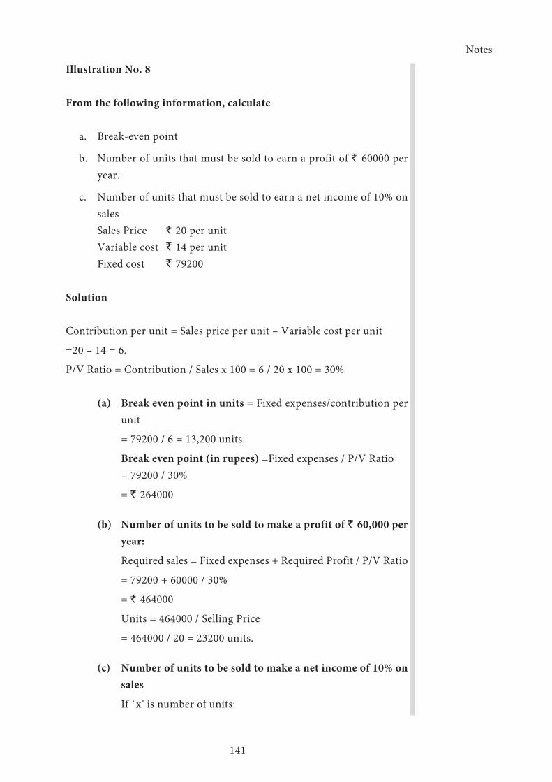
Notes

141

Illustration No. 8

From the following information, calculate

a. Break-even point

b. Number of units that must be sold to earn a profit of ` 60000 per year.

c. Number of units that must be sold to earn a net income of 10% on salesSales Price ` 20 per unitVariable cost ` 14 per unitFixed cost ` 79200

Solution

Contribution per unit = Sales price per unit – Variable cost per unit

=20 – 14 = 6.

P/V Ratio = Contribution / Sales x 100 = 6 / 20 x 100 = 30%

(a) Break even point in units = Fixed expenses/contribution per unit

= 79200 / 6 = 13,200 units.

Break even point (in rupees) =Fixed expenses / P/V Ratio = 79200 / 30%

= ` 264000

(b) Number of units to be sold to make a profit of ` 60,000 per year:

Required sales = Fixed expenses + Required Profit / P/V Ratio

= 79200 + 60000 / 30%

= ` 464000

Units = 464000 / Selling Price

= 464000 / 20 = 23200 units.

(c) Number of units to be sold to make a net income of 10% on sales

If `x’ is number of units:

Notes

142

20x = Fixed Cost + Variable Cost + Profit

20x = 79200 + 14x + 2x

20x – 16x = 79200

x = 79200 / 4 = 19800 units

Proof: Sales = 19800 x 20 = 396000 less: Variable cost 19800 x 14 = 277200 ------------Contribution = 118000Less: Fixed Cost = 79200 ------------Profit = 39600 ------------

Profit as a % of sales = 39600 / 396000 x 100 = 10%

Illustration No. 9

You are given the following data for the year 1986 for a factory.

Output: 40000 units

Fixed expenses: ` 200000

Variable cost per unit: ` 10

Selling price per unit: ` 20

How many units must be produced and sold in the year 1987, if it is anticipated that selling price would be reduced by 10%, variable cost would be ` 12 per unit, and fixed cost will increase by 10%? The factory would like to make a profit in 1987 equal to that of the profit in 1986.

Notes

143

Solution

Margin Cost and contribution statement for the year 1986

Particulars `

Sales 40,000 x 20 8,00,000

Less: Variable Cost 40,000 x 10

4,00,000

Contribution 4,00,000

Less: Fixed Cost 2,00,000

Profit 2,00,000

Calculation of units to be produced and sold in 1987 to make the same profit as in 1986:

New Selling Price=20 – (20 x 10%) = 20 – 2 = ` 18

New variable cost = ` 12 (given New fixed cost=200000 + (200000 x 10%)

=200000 + 20000 = 220000

New P/V Ratio=Sales – Variable Cost / Sales x 100

=18 – 12 / 18 x 100 = 33 1/3 %

Required sales=Required profit + Fixed expenses / P/V Ratio

=200000 + 220000 / 33 1/3 % =` 1260000

Units to be sold=Required Sales / New Selling Price

=1260000 / 18 = 70,000 units.

Illustration No. 10

The P/V Ratio of a firm dealing in precision instruments is 50% and margin of safety is 40%. You are required to work-out break even point and the net profit if the sales volume is ` 5000000. If 25% of variable cost is labour cost, what will be the effect on BEP and profit when labour efficiency decreases by 5%.

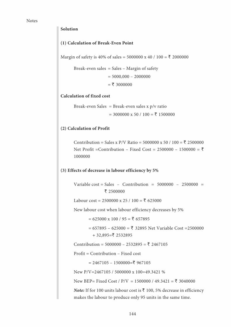
Notes

144

Solution

(1) Calculation of Break-Even Point

Margin of safety is 40% of sales = 5000000 x 40 / 100 = ` 2000000

Break-even sales = Sales – Margin of safety

= 5000,000 – 2000000

= ` 3000000

Calculation of fixed cost

Break-even Sales = Break-even sales x p/v ratio

= 3000000 x 50 / 100 = ` 1500000

(2) Calculation of Profit

Contribution = Sales x P/V Ratio = 5000000 x 50 / 100 = ` 2500000Net Profit =Contribution – Fixed Cost = 2500000 – 1500000 = `

1000000

(3) Effects of decrease in labour efficiency by 5%

Variable cost = Sales – Contribution = 5000000 – 2500000 = ` 2500000

Labour cost = 2500000 x 25 / 100 = ` 625000

New labour cost when labour efficiency decreases by 5%

= 625000 x 100 / 95 = ` 657895

= 657895 – 625000 = ` 32895 Net Variable Cost =2500000 + 32,895=` 2532895

Contribution = 5000000 – 2532895 = ` 2467105

Profit = Contribution – Fixed cost

= 2467105 – 1500000=` 967105

New P/V=2467105 / 5000000 x 100=49.3421 %

New BEP= Fixed Cost / P/V = 1500000 / 49.3421 = ` 3040000

Note: If for 100 units labour cost is ` 100, 5% decrease in efficiency makes the labour to produce only 95 units in the same time.

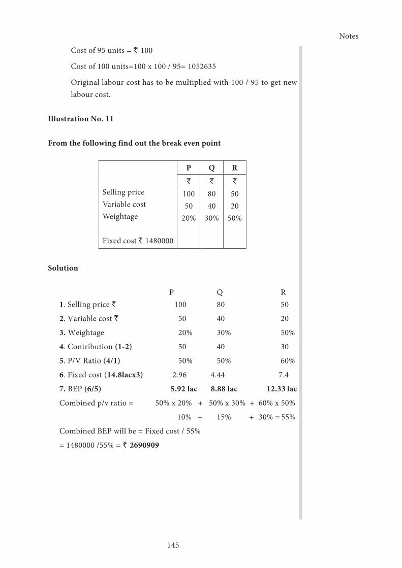
Notes

145

Cost of 95 units = ` 100

Cost of 100 units=100 x 100 / 95= 1052635

Original labour cost has to be multiplied with 100 / 95 to get new labour cost.

Illustration No. 11

From the following find out the break even point

Selling price Variable cost Weightage

Fixed cost ` 1480000

P Q R

`

10050

20%

`

8040

30%

`

5020

50%

Solution

P Q R1. Selling price ` 100 80 50

2. Variable cost ` 50 40 20

3. Weightage 20% 30% 50%

4. Contribution (1-2) 50 40 30

5. P/V Ratio (4/1) 50% 50% 60%

6. Fixed cost (14.8lacx3) 2.96 4.44 7.4

7. BEP (6/5) 5.92 lac 8.88 lac 12.33 lac

Combined p/v ratio = 50% x 20% + 50% x 30% + 60% x 50%

10% + 15% + 30% = 55%

Combined BEP will be = Fixed cost / 55%

= 1480000 /55% = ` 2690909

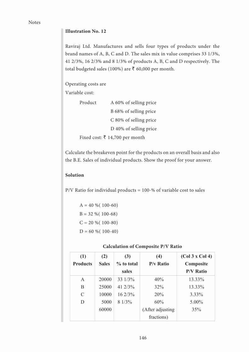
Notes

146

Illustration No. 12

Raviraj Ltd. Manufactures and sells four types of products under the brand names of A, B, C and D. The sales mix in value comprises 33 1/3%, 41 2/3%, 16 2/3% and 8 1/3% of products A, B, C and D respectively. The total budgeted sales (100%) are ` 60,000 per month.

Operating costs are

Variable cost:

Product A 60% of selling price

B 68% of selling price

C 80% of selling price

D 40% of selling price

Fixed cost: ` 14,700 per month

Calculate the breakeven point for the products on an overall basis and also the B.E. Sales of individual products. Show the proof for your answer.

Solution

P/V Ratio for individual products = 100-% of variable cost to sales

A = 40 %( 100-60)

B = 32 %( 100-68)

C = 20 %( 100-80)

D = 60 %( 100-40)

Calculation of Composite P/V Ratio

(1)Products

(2)Sales

(3)% to total

sales

(4) P/v Ratio

(Col 3 x Col 4) Composite P/V Ratio

ABCD

20000 25000 10000 5000

60000

33 1/3% 41 2/3% 16 2/3% 8 1/3%

40% 32% 20% 60%

(After adjusting fractions)

13.33% 13.33% 3.33% 5.00% 35%

Notes

147

Total Fixed costComposite BEP in ` = ----------------------------

Composite P / V Ratio ` 14,700

= ------------- = ` 42,000 35%

Proof of validity of composite B.E.P

Break even sales of:

A ` 42000 x 33 1/3 % = ` 14000 14000 x 40% = 5600

B ` 42000 x 41 2/3 % = ` 17500 17500 x 32% = 5600

C ` 42000 x 16 2/3 % = ` 7000 7000 x 20% = 1400

D ` 42000 x 8 1/3 % = ` 3500 3500 x 60% = 2100

Total contribution 14700

Total fixed cost 14700

Profit/Loss Nil

****

Notes

148

Lesson 3.3 - Marginal Costing and Decision-Making

Introduction

During normal circumstances, Price is based on full cost and a certain desired margin, or profit. But in certain special circumstances, products are to be sold at a price below total cost based on absorption costing.

In such circumstances, the price should be fixed on the basis of marginal cost so as to cover the marginal cost and contribute something towards fixed cost. Sometimes it becomes necessary to reduce the selling price to the level of marginal cost.

The most useful contribution of marginal costing is that it helps management in vital decision making. Decision making essentially involves a choice between various alternatives and marginal costing assists in choosing the best alternative by furnishing all possible facts. The information supplied by marginal costing technique is of special importance, where information obtained from total absorption costing method is incomplete.

The following are some of the managerial decisions which are taken with the help of marginal costing decisions:

➢ Fixation of selling price.

➢ Make or buy decision

➢ Selection of a suitable product mix or sales mix.

➢ Key factor:

➢ Alternative methods of production.

➢ Profit planning

➢ Suspending activities i.e., closing down

Notes

149

Fixation of Selling Price

One of the main purposes of cost accounting is the ascertainment of cost for fixation of selling price. Price fixation is one of the fundamental problems which the management has to face. Although prices are determined by market conditions and other factors, marginal costing technique assists the management in the fixation of selling prices under various circumstances which is as follows.

a) Pricing under normal conditions.

b) Pricing during stiff competition.

c) Pricing during trade depression.

d) Accepting special bulk orders.

e) Accepting additional orders to utilize idle capacity.

f ) Accepting orders and exporting new materials.

Decision to Make or Buy

It is a common type of business decision for a company to determine whether to make to buy materials or component parts. Manufacturing or making often requires a capital investment so that a decision to make must always be made whenever the expected cost savings provide a higher return on the required capital investment that can be obtained by employing these funds in an alternative investment bearing the same risk. In practice, difficulties are encountered in identifying and estimating relevant costs and in calculating non-cost considerations.

In case a firm decides to get a product manufactured from outside, besides savings in cost, it must also take into account the following factors:

1. Whether the outside supplier would be in a position to maintain the quality of the product?

2. Whether the supplier would be regular in his supplies?

3. Whether the supplier is reliable? In other words is the financially and technically sound?

Notes

150

Selection of a Suitable Product Mix or Sales Mix

When a concern manufactures a number of products a problem often raises as to which product mix or sales mix will give the maximum profit. In other words, what should be the best combination of varying quantities of the different products/? Which would be selected from amongst the various alternative combinations available? Such a problem can be solved with the help of marginal contribution cost analysis: the product mix which gives the best optimum mix. Eg, let us consider the following analysis made in respect of three products manufactured in a company:

Product I (`) Product II (`) Product III (`)Per unit sales priceMaterialsLabourVariable OverheadsMarginal costMarginal contribution

25 6 5 41510

30 8 4 31515

18 2 6 513 5

Out of the three products, product II gives the highest contribution per unit. Therefore, if no other factors no others factors intervene, the production capacity will be utilized to the maximum possible extent for the manufacture of that product. Product I ranks second and so, after meeting the requirement of Product II, the capacity will be utilized for product I. What ever capacity is available thereafter may be utilized for Product III.

Key Factor

Firms would try to produce commodities which fetch a higher contribution or the highest contribution. This assumption is based on the possibility of selling out the product at the maximum. Sometimes it may happen that the firm may not be able to push out all products manufactured. And, sometimes the firm may not be able to sell all the products it manufactured or production may be limited due to shortage of materials, labour, plant, capacity, capital, demand, etc.

Notes

151

A key factor is also called as a limiting factor or principal budget factor or scarce factor. It is a factor of production which is scarce and because of want of which the production may stop. Generally sales volume, plant capacity, material, labour etc may be limiting factors. When there is a key factor profit is calculated by using the formula

ContributionProfitability = -------------------------------------------------

Key factor (Materials, Labour, or Capital)

When there is no limiting factor, the production can be on the basis of the highest P / V ratio. When two or more limiting factors are in operation, they will be seriously considered to determine the profitability.

Alternative Methods of Production

Sometimes management has to choose from among alternative methods of production, i.e., mechanical or manual. In such circumstances, the technique of marginal costing can be applied and the method which gives the highest contribution can be adopted.

Profit Planning

Profit planning is the planning of the future operations to attain maximum profit or to maintain level of profit. Whenever there is a change in sale price, variable costs and product mix, the required volume of sales for maintaining or attaining a desired amount of profit may be ascertained with the help of P / V ratio.

Fixed Cost + Profit Expected Sales = -------------------------

P / V Ratio

Suspending Activities i.e., closing down

When a firm is operating for loss sometime, the management has to decide upon its shut down.

Notes

152

i) Complete shut down:

ii) When the selling price does not even cover the variable cost: or

iii) The demand for the output is very low and the future prospects are bleak.

Complete shutdown saves the management from the fixed of running the factory or division or firm.

b) Partial or temporary shutdown: Here the intention is to close down for some time and reopen the firm when circumstances favour it. Some fixed cost will continue in the form of irreducible minimum, like Skelton staff to maintain the factory, some managerial remuneration, salaries, irreplaceable technical experts, etc. The saving from the partial shutdown should be compared with the position if the firm continues. If there is substantial savings, shut down may be preferable. Minor savings in expenditure does not warrant shut down because reviving a firm is a cumbersome process.

Decision to Make or Buy

Illustration No. 1

An automobile manufacturing company finds that the cost of making Part No. 208 in its own workshop is ` 6. The same part is available in the market at ` 5.60 with an assurance of continuous supply. The cost data to make the part are:

Material ` 2.00

Direct labour ` 2.50

Other variable cost ` 0.50

Fixed cost allocated ` 1.00 ------- ` 6.00 -------

Should be part be made or brought?

Will your answer be different if the market price is ` 4.60? Show your calculations clearly.

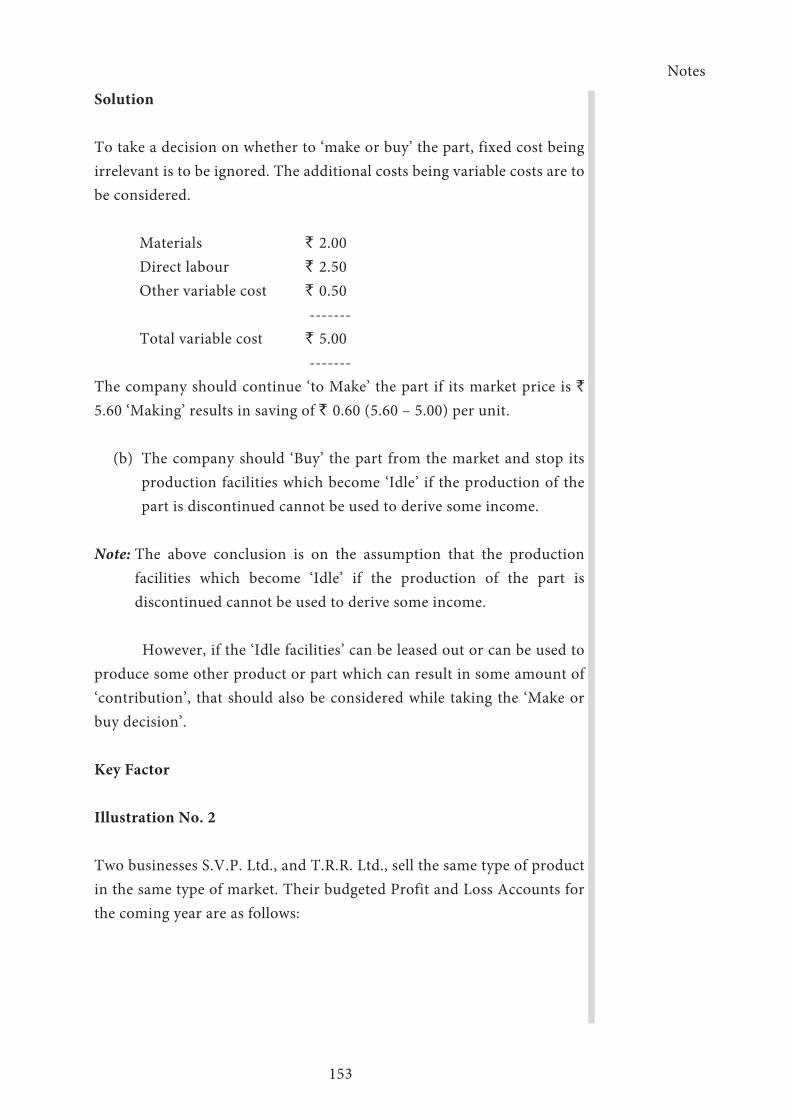
Notes

153

Solution

To take a decision on whether to ‘make or buy’ the part, fixed cost being irrelevant is to be ignored. The additional costs being variable costs are to be considered.

Materials ` 2.00Direct labour ` 2.50Other variable cost ` 0.50 -------Total variable cost ` 5.00 -------

The company should continue ‘to Make’ the part if its market price is `

5.60 ‘Making’ results in saving of ` 0.60 (5.60 – 5.00) per unit.

(b) The company should ‘Buy’ the part from the market and stop its production facilities which become ‘Idle’ if the production of the part is discontinued cannot be used to derive some income.

Note: The above conclusion is on the assumption that the production facilities which become ‘Idle’ if the production of the part is discontinued cannot be used to derive some income.

However, if the ‘Idle facilities’ can be leased out or can be used to produce some other product or part which can result in some amount of ‘contribution’, that should also be considered while taking the ‘Make or buy decision’.

Key Factor

Illustration No. 2

Two businesses S.V.P. Ltd., and T.R.R. Ltd., sell the same type of product in the same type of market. Their budgeted Profit and Loss Accounts for the coming year are as follows:

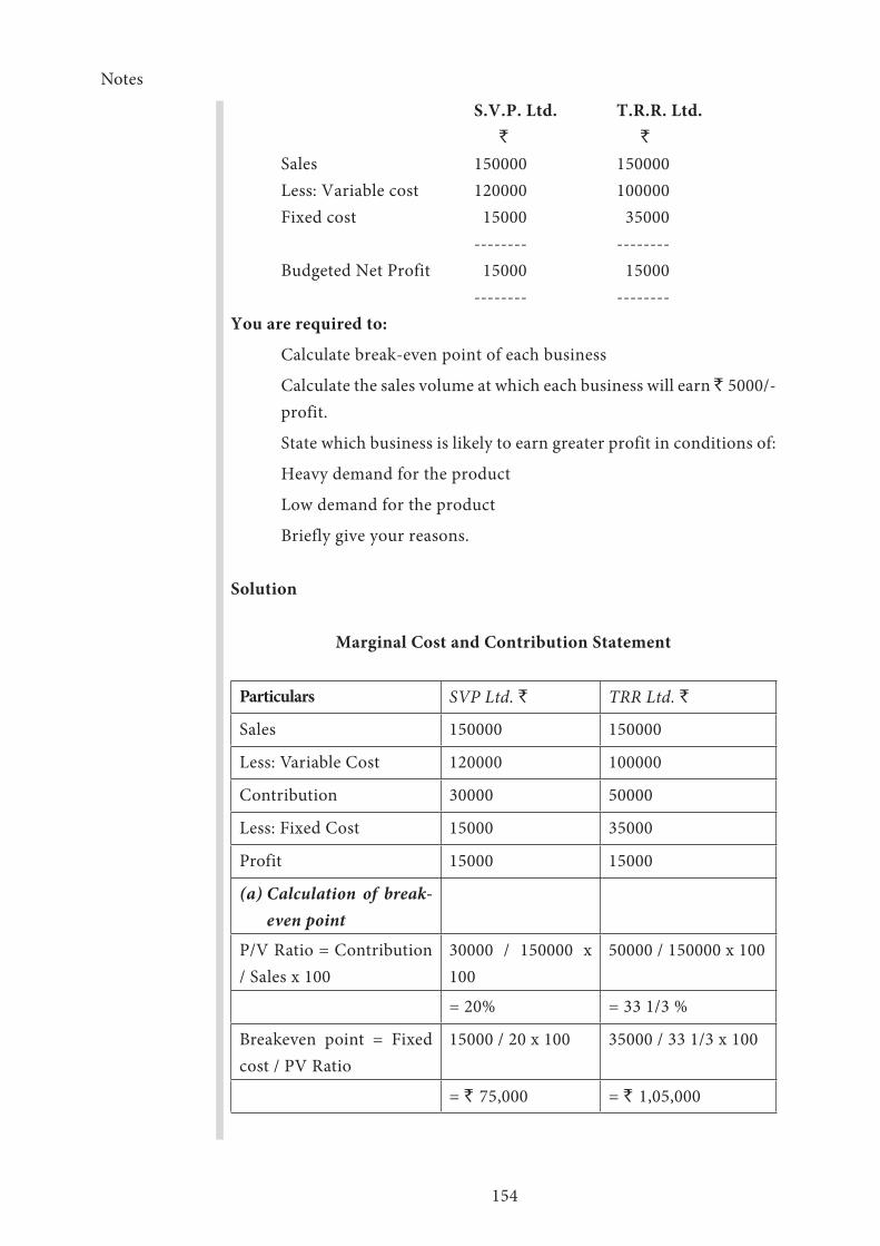
Notes

154

S.V.P. Ltd. T.R.R. Ltd. ` `

Sales 150000 150000Less: Variable cost 120000 100000Fixed cost 15000 35000 -------- --------Budgeted Net Profit 15000 15000 -------- --------

You are required to:

Calculate break-even point of each business

Calculate the sales volume at which each business will earn ̀ 5000/- profit.

State which business is likely to earn greater profit in conditions of:

Heavy demand for the product

Low demand for the product

Briefly give your reasons.

Solution

Marginal Cost and Contribution Statement

Particulars SVP Ltd. ` TRR Ltd. `

Sales 150000 150000

Less: Variable Cost 120000 100000

Contribution 30000 50000

Less: Fixed Cost 15000 35000

Profit 15000 15000

(a) Calculation of break-even point

P/V Ratio = Contribution / Sales x 100

30000 / 150000 x 100

50000 / 150000 x 100

= 20% = 33 1/3 %

Breakeven point = Fixed cost / PV Ratio

15000 / 20 x 100 35000 / 33 1/3 x 100

= ` 75,000 = ` 1,05,000

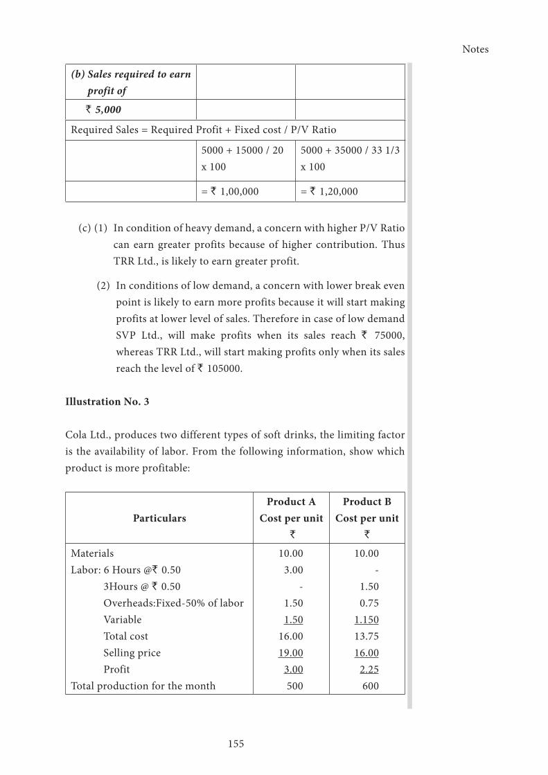
Notes

155

(b) Sales required to earn profit of

` 5,000

Required Sales = Required Profit + Fixed cost / P/V Ratio

5000 + 15000 / 20 x 100

5000 + 35000 / 33 1/3 x 100

= ` 1,00,000 = ` 1,20,000

(c) (1) In condition of heavy demand, a concern with higher P/V Ratio can earn greater profits because of higher contribution. Thus TRR Ltd., is likely to earn greater profit.

(2) In conditions of low demand, a concern with lower break even point is likely to earn more profits because it will start making profits at lower level of sales. Therefore in case of low demand SVP Ltd., will make profits when its sales reach ` 75000, whereas TRR Ltd., will start making profits only when its sales reach the level of ` 105000.

Illustration No. 3

Cola Ltd., produces two different types of soft drinks, the limiting factor is the availability of labor. From the following information, show which product is more profitable:

Particulars

Product A Cost per unit

`

Product B Cost per unit

`

MaterialsLabor: 6 Hours @` 0.50 3Hours @ ` 0.50 Overheads:Fixed-50% of labor Variable Total cost Selling price ProfitTotal production for the month

10.003.00

-1.501.50

16.0019.00

3.00500

10.00-

1.500.75

1.15013.7516.00

2.25600

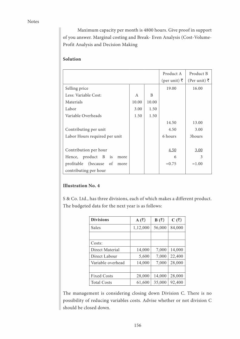
Notes

156

Maximum capacity per month is 4800 hours. Give proof in support of you answer. Marginal costing and Break- Even Analysis (Cost-Volume-Profit Analysis and Decision Making

Solution

Product A(per unit) `

Product B(Per unit) `

Selling priceLess: Variable Cost:MaterialsLaborVariable Overheads

Contributing per unit Labor Hours required per unit

Contribution per hourHence, product B is more profitable (because of more contributing per hour

A10.00

3.001.50

B10.00

1.501.50

19.00

14.504.50

6 hours

4.506

=0.75

16.00

13.003.00

3hours

3.003

=1.00

Illustration No. 4

S & Co. Ltd., has three divisions, each of which makes a different product. The budgeted data for the next year is as follows:

Divisions A (`) B (`) C (`)

Sales 1,12,000 56,000 84,000

Costs:Direct Material 14,000 7,000 14,000Direct Labour 5,600 7,000 22,400Variable overhead 14,000 7,000 28,000

Fixed Costs 28,000 14,000 28,000Total Costs 61,600 35,000 92,400

The management is considering closing down Division C. There is no possibility of reducing variables costs. Advise whether or not division C should be closed down.

Notes

157

Solution

Divisions A (`) B (`) C (`)

Sales 112000 56000 84000

Less: Variable Costs:

Direct Material 14000 7000 14000

Direct Labour 5600 7000 22400

Variable overhead 14000 7000 28000

33600 21000 64000

78400 35000 20000

Less: Fixed Costs 28000 14000 28000

Loss 50400 21000 8000

Since Division C is giving a positive contribution of ` 20000/- it should not be discharged.

Export Decision

Export decision may arise when large scale purchasers demand products at a price which is less than the market price. A decision has to be taken now whether to accept the order to reject it. By reducing the normal price, the volume of output and the sales can be increased. If the price is below the total cost, rejection of the order is aimed at.

Illustration No. 5

Due to industrial depression, a plant is running at present, at 50% of its capacity. The following details are available.

Cost of Production per Unit

Direct materials ` 3

Direct labour ` 1

Variable overhead ` 2

Fixed overhead ` 2 ` 8

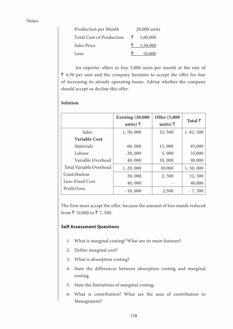
Notes

158

Production per Month 20,000 units

Total Cost of Production ` 1,60,000

Sales Price ` 1,50,000

Loss: ` 10,000 An exporter offers to buy 5,000 units per month at the rate of ` 6.50 per unit and the company hesitates to accept the offer for fear of increasing its already operating losses. Advise whether the company should accept or decline this offer.

Solution

Existing (20,000 units) `

Offer (5,000 units) `

Total `

Sales Variable Cost: Materials Labour Variable Overhead

Total Variable OverheadContributionLess: Fixed CostProfit/Loss

1, 50, 000

60, 000 20, 000 40, 000

32, 500

15, 000 5, 000

10, 000

1, 82, 500

85,00055,00090,000

1, 20, 000 30,000 1, 50, 000

30, 000 40, 000

2, 500 -

32, 50040,000

- 10, 000 2,500 - 7, 500

The firm must accept the offer, because the amount of loss stands reduced from ` 10,000 to ` 7, 500.

Self Assessment Questions

1. What is marginal costing? What are its main features?

2. Define marginal cost?

3. What is absorption costing?

4. State the differences between absorption costing and marginal costing.

5. State the limitations of marginal costing.

6. What is contribution? What are the uses of contribution to Management?

Notes

159

7. What is margin of safety? How is it calculated?

8. What is angle of incidence? What does it indicate?

9. What are the advantages and disadvantages of marginal costing?

10. The selling price of a particular product is ` 100 and the marginal cost is ` 65. During the month of April, 800 units produced of which 500 were sold. There was no opening at the commencement of the month. Fixed costs amounted to ̀ 18000. Provide a statement using a) Marginal costing and b) Absorption costing, showing the closing stock valuation and the profit earned under each principle.

11. From the following information, calculate the amount of contribution and profit.

`

Sales 1000000

Variable cost 600000

Fixed cost 150000

12. Determine the amount of fixed cost from the following.

`

Sales 300000

Variable cost 200000

Profit 50000

13. Determine the amount of variable cost from the following.

`

Sales 500000

Fixed cost 100000

Profit 100000

14. Discuss the role of marginal costing in taking managerial decisions.

15. What is key factor? What is it importance?

16. Explain the different factors to be considered while taking a make or buy decision.

17. When is selling below cost is permissible or necessary?

18. How do you decide upon the optimal sales mix?

160

19. Present the following information to management:

The managerial product cost and the contribution per unit and

ii. The total contribution and profits resulting from each of the sales mixes:

Product per unit

`

Direct materials A 10

Direct materials B 9

Direct wages A 3

Direct wages B 2

Fixed expenses - ` 800

(Variable expenses are allotted to products 100% of direct wages)

Sales Price - A ` 20

Sales Price - B ` 15

Sales mix:

100 units of product A and 200 of B

150 units of product B and 150 of B

200 unit of product A and 100 of B

Recommend which of the sales mixes should be adopted.

20. Pondicherry Trading Corporation is running its plant at 50% capacity. The management has supplied you the following details:

Cost of Production

Per Unit (`)

Direct materials 4

Direct labour 2

Variable overheads 6

Fixed overheads (Fully absorbed) 4

16

Production per month 40000 units

Total cost of production

40000 X ` 16 640000

Sales price 40000 X ` 14 560000

` 80000

Notes

161

An exporter offers to purchase 10000 units per month at ` 13 per unit and the company is hesitating in accepting the offer due to the fear that it will increase its already large operating losses.

Advise whether the company should accept or decline this offer.

21. What is break even point? How do you calculate it?

22. What do you understand by cost volume profit analysis? What is its significance?

23. What is composite break even point?

24. What is a break even chart? How isit useful?

25. Mention the assumptions underlying a break even chart?

26. Calculate BEP in units and value for the following:

Total cost ` 50000

Total variable cost ` 30000

Sales (5000 units) ` 50000

27. A Ltd. has two factories X and Y producing same article whose selling price is ` 150 per unit. Other details are:

X Y

Capacity in units 10000 15000

Variable cost per unit (`) 100 120

Fixed expenses (`) 300000 210000

Determine the BEP for the two factories assuming constant sales mix also composite BEP.

28. From the following data calculate

a. Break even point (Units)

b. If sales are 10% and 15% above the break even sales volume determine the net profit.

Selling price per unit - ` 10

Direct material per unit - ` 3

Fixed overheads - ` 10000

Variable overheads per unit – ` 2

Direct labour cost per unit - ` 2

****

162

Notes

163

UNIT - IV

Learning Objectives

After reading this Unit you will be able to

➢ Understand the concept of DuPont analysis and some important ratios

➢ Know the concept, meaning of funds and familiarize with various technical terms, meaning, and concepts of funds flow statement

➢ Understand the steps to prepare funds flow statement

➢ Prepare cash flow statement

➢ Develop the power of understanding the important issues in the area of Management Accounting

➢ Decide the use of costing in Management Accounting

Unit Structure

Lesson 4.1 - DU-Pont Analysis

Lesson 4.2 - Funds Flow Analysis

Lesson 4.3 - Cash Flow Analysis

Lesson 4.4 - Contemporary Issues in Management

Notes

164

Lesson - 4.1 - DU-Pont Analysis

Introduction

The Du Pont Company of USA introduced this analysis in 1920s. This analysis acquired wider acceptance at the industry level. The Du Pont analysis is an extension of return on investment ratio. This analysis is considered to be an important tool to evaluate the managerial performance by relating the net profit and assets turnover.

The Du Pont chart is mainly based on two components i.e., net profit and capital employed. Net profit is related to operating expenses. If the expenses are within the control then this cost control will definitely reflect in profit margin. Capital employed, on the other hand, consists of current assets and net fixed assets. This analysis is a useful one in segregation and identification of factors that affect the overall performance of the company.

Important Ratios and their Application Current Ratio

Current ratio establishes the relationship between current assets and current liabilities. It is important component to know the short term solvency of the firm. Generally firms have a lot of short term financial obligations. In order to meet out these obligations, the firm shall have to have adequate short term financial liquidity. This liquidity is indicated by current assets available in the company. Suppose a firm’s current ratio is high, it means the firm is capable of meeting its current obligations without any difficulty. There is rule of thumb on current assets and current liabilities level. According to that the rule of thumb is 2:1 that means if a firm has current asset of ` 2, it can have current liabilities of ` 1. The current ratio is calculated as follows.

Current ratio =

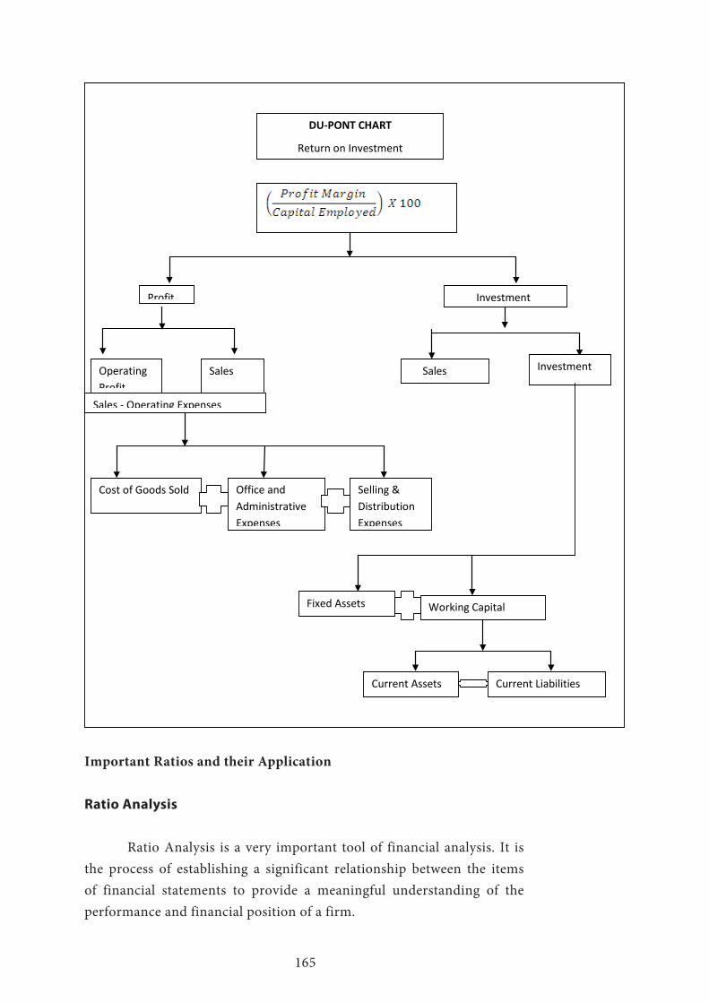
165

DU-PONT CHART

Return on Investment

Profit Investment Turnover

Operating Profit

Sales

Sales - Operating Expenses

Sales Investment

Cost of Goods Sold Office and Administrative Expenses

Selling & Distribution Expenses

Fixed Assets Working Capital

Current Assets Current Liabilities

Important Ratios and their Application

Ratio Analysis

Ratio Analysis is a very important tool of financial analysis. It is the process of establishing a significant relationship between the items of financial statements to provide a meaningful understanding of the performance and financial position of a firm.

Notes

166

Meaning of Ratio

Since, we are using the term ‘ratio’ in relation to financial statement analysis; it may properly mean ‘An Accounting Ratio’ or ‘Financial Ratio’. It may be defined as the mathematical expression of the relationship between two accounting figures. But these figures must be related to each other (i.e., these figures must have a mutual cause and effect relationship) to produce a meaningful and useful ratio. For example, the figure of turnover cannot be said to be significantly related to the figure of share premium. It indicates a quantitative relationship which the analyst may use to make a qualitative judgment about the various aspects of the financial position and performance of a concern. It may be expressed as a percentage or as a rate (i.e., in ‘x’ number of times) or as a pure ratio, e.g., if gross profit on sales of ` 1,00,000 is ` 20,000, the ratio of gross profit to sales is 20%. i.e ` 20,000

` 1,00,000 X 100

In another example of Capital Turnover Ratio, if Sales with a Capital Employed of ` 20,000 is ` 1, 00,000, the Capital Turnover Ratio may be expressed as 5 times i.e., ` 1, 00,000 / ` 20,000. In the case of a Current Ratio, if current assets are ` 1,00,000 and current liabilities are `

50,000, Current Ratio may be expressed as 2: 1 i.e., ` 1,00,000: ` 50,000.

In view of the requirements of various users (e.g., Short-term Creditors, Long-term Creditors, Management, Investors) of the ratios, one may classify the ratios into the following four groups, such as Liquidity Ratios, Solvency Ratios, Activity Ratios and Profitability Ratios.

Liquidity Ratios

These ratios measure the concern’s ability to meet short-term obligations as and when they become due. These ratios show the short-term financial solvency of the concern. Usually the following two ratios are calculated for this purpose:

1. Current Ratio and 2. Quick Ratio

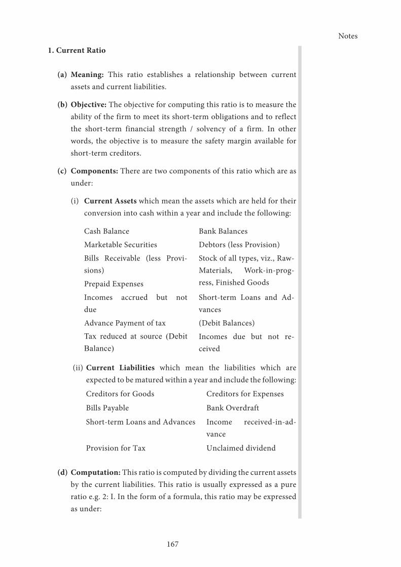
Notes

167

1. Current Ratio

(a) Meaning: This ratio establishes a relationship between current assets and current liabilities.

(b) Objective: The objective for computing this ratio is to measure the ability of the firm to meet its short-term obligations and to reflect the short-term financial strength / solvency of a firm. In other words, the objective is to measure the safety margin available for short-term creditors.

(c) Components: There are two components of this ratio which are as under:

(i) Current Assets which mean the assets which are held for their conversion into cash within a year and include the following:

Cash Balance Bank Balances

Marketable Securities Debtors (less Provision)

Bills Receivable (less Provi-sions)

Stock of all types, viz., Raw-Materials, Work-in-prog-ress, Finished GoodsPrepaid Expenses

Incomes accrued but not due

Short-term Loans and Ad-vances

Advance Payment of tax (Debit Balances)

Tax reduced at source (Debit Balance)

Incomes due but not re-ceived

(ii) Current Liabilities which mean the liabilities which are expected to be matured within a year and include the following:

Creditors for Goods Creditors for Expenses

Bills Payable Bank Overdraft

Short-term Loans and Advances Income received-in-ad-vance

Provision for Tax Unclaimed dividend

(d) Computation: This ratio is computed by dividing the current assets by the current liabilities. This ratio is usually expressed as a pure ratio e.g. 2: I. In the form of a formula, this ratio may be expressed as under:

Notes

168

Current AssetsCurrent Ratio = ---------------------------

Current Liabilities

(e) Interpretation: It indicates rupees of current assets available for each rupee of current liability, Higher the ratio, greater the margin of safety for short-term creditors and vice-versa. However, too high / too low ratio calls for further investigation since the too high ratio may indicate the presence of idle funds with the firm or the absence of investment opportunities with the firm and too low ratio may indicate the over trading/under capitalization if the capital turnover ratio is high.

Traditionally, a current ratio of 2: 1 is considered to be a satisfactory ratio. On the basis of this traditional rule, if the current ratio is 2 or more, it means the firm is adequately liquid and has the ability to meet its current obligations but if the current ratio is less than 2, it means the firm may have difficulty in meeting its current obligations. The logic behind this rule is that even if the value of current assets becomes half, the firm can still meet its short-term obligations.

However, the traditional standard of 2: I should not be used blindly since there may be firms having current ratio of less than 2, and may be working efficiently and meeting their short-term obligations as and when they become due while the other firms having current ratio of more than 2, may not be able to meet their current obligations in time. This is so because the current ratio measures the quantity of current assets and not their quality. Current assets may consist of doubtful and slow paying debtors and slow moving and obsolete stock of goods. That is why, it can be said that current ratio is no doubt a quick measurement of a firm’s liquidity but it is crude as well.

(f) Precaution: While computing and using the current ratio, it must be ensured that (a) the quality of both receivables (debtors and bills receivable) and inventory have been carefully assessed and (b) that all current assets and current liabilities have been properly valued.

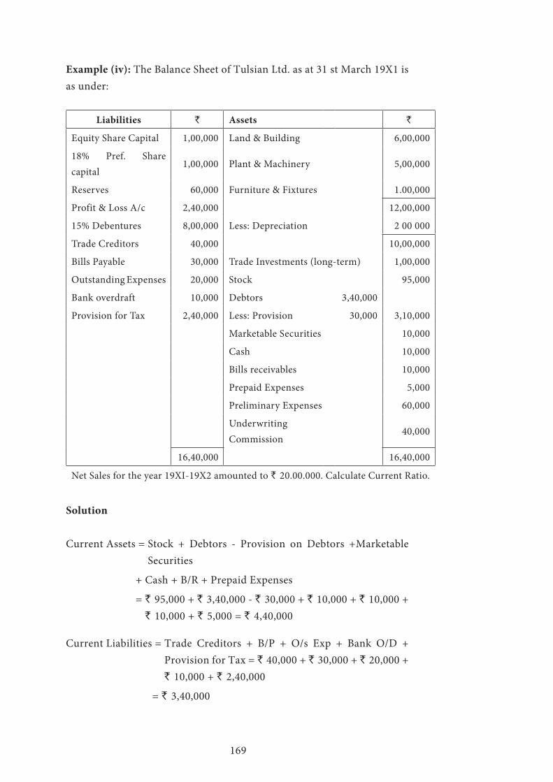
169

Example (iv): The Balance Sheet of Tulsian Ltd. as at 31 st March 19X1 is as under:

Liabilities ` Assets `

Equity Share Capital 1,00,000 Land & Building 6,00,000

18% Pref. Share capital

1,00,000 Plant & Machinery 5,00,000

Reserves 60,000 Furniture & Fixtures 1.00,000

Profit & Loss A/c 2,40,000 12,00,000

15% Debentures 8,00,000 Less: Depreciation 2 00 000

Trade Creditors 40,000 10,00,000

Bills Payable 30,000 Trade Investments (long-term) 1,00,000

Outstanding Expenses 20,000 Stock 95,000

Bank overdraft 10,000 Debtors 3,40,000

Provision for Tax 2,40,000 Less: Provision 30,000 3,10,000

Marketable Securities 10,000

Cash 10,000

Bills receivables 10,000

Prepaid Expenses 5,000

Preliminary Expenses 60,000

Underwriting Commission

40,000

16,40,000 16,40,000

Net Sales for the year 19XI-19X2 amounted to ` 20.00.000. Calculate Current Ratio.

Solution

Current Assets = Stock + Debtors - Provision on Debtors +Marketable Securities

+ Cash + B/R + Prepaid Expenses

= ̀ 95,000 + ` 3,40,000 - ` 30,000 + ` 10,000 + ` 10,000 + ` 10,000 + ` 5,000 = ` 4,40,000

Current Liabilities = Trade Creditors + B/P + O/s Exp + Bank O/D + Provision for Tax = ` 40,000 + ` 30,000 + ` 20,000 + ` 10,000 + ` 2,40,000

= ` 3,40,000

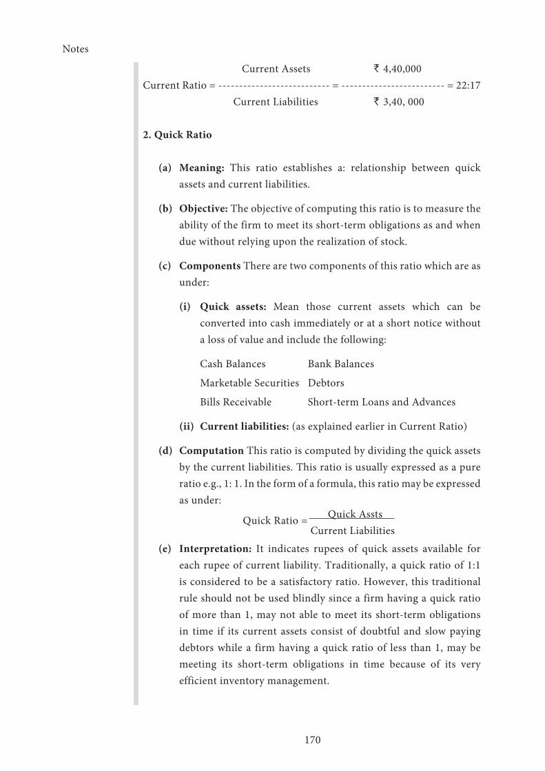
Notes

170

Current Assets ` 4,40,000Current Ratio = --------------------------- = ------------------------- = 22:17 Current Liabilities ` 3,40, 000

2. Quick Ratio

(a) Meaning: This ratio establishes a: relationship between quick assets and current liabilities.

(b) Objective: The objective of computing this ratio is to measure the ability of the firm to meet its short-term obligations as and when due without relying upon the realization of stock.

(c) Components There are two components of this ratio which are as under:

(i) Quick assets: Mean those current assets which can be converted into cash immediately or at a short notice without a loss of value and include the following:

Cash Balances Bank Balances

Marketable Securities Debtors

Bills Receivable Short-term Loans and Advances

(ii) Current liabilities: (as explained earlier in Current Ratio)

(d) Computation This ratio is computed by dividing the quick assets by the current liabilities. This ratio is usually expressed as a pure ratio e.g., 1: 1. In the form of a formula, this ratio may be expressed as under:

Quick Assts Quick Ratio = Current Liabilities

(e) Interpretation: It indicates rupees of quick assets available for each rupee of cur rent liability. Traditionally, a quick ratio of 1:1 is considered to be a satisfactory ratio. However, this traditional rule should not be used blindly since a firm having a quick ratio of more than 1, may not able to meet its short-term obligations in time if its current assets consist of doubtful and slow paying debtors while a firm having a quick ratio of less than 1, may be meeting its short-term obligations in time because of its very efficient inventory management.

Notes

171

(f) Precaution: While computing and using the quick ratio, it must be ensured, (a) that the quality of the receivables (debtors and bills receivable) has been carefully assessed and (b) that all quick assets and current liabilities have been properly valued.

Example (v): Current Assets ` 2,00,000, Inventory ` 40,000, Working Capital ` 1, 20 000. Calculate the Quick Ratio.

Solution: Current Liabilities = Current Assets - Working Capital

= ` 2,00,000 - ` 1,20,000 = ` 80,000

Quick Assets = Current Assets - Inventory

= ` 2,00,000 - ` 40,000 = ` 1,60,000

Quick Assets ` l,60,000 Quick Ratio = --------------------- --------------------- = 2:1

Current Liabilities ` 80000

Solvency Ratios

These ratios show the long-term financial solvency and measure the enterprise’s ability to pay the interest regularly and to repay the principal (i.e. capital amount) on maturity or in pre-determined installments at due dates. Usually, the following ratios are calculated to judge the long-term financial solvency of the concern.

Debt-Equity Ratio

(a) Meaning: This ratio establishes a relationship between long-term debts and share-holders’ funds.

(b) Objective: The objective of computing this ratio is to measure the relative proportion of debt and equity in financing the assets of a firm.

(c) Components: There are two components of this ratio, which are as under:

(i) Long-term Debts, which mean long-term loans (whether secured or unsecured (e.g., Debentures, bonds, loans from financial institutions).

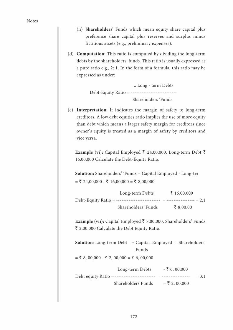
Notes

172

(ii) Shareholders’ Funds which mean equity share capital plus preference share capital plus reserves and surplus minus fictitious assets (e.g., preliminary expenses).

(d) Computation: This ratio is computed by dividing the long-term debts by the share holders’ funds. This ratio is usually expressed as a pure ratio e.g., 2: 1. In the form of a formula, this ratio may be expressed as under:

.. Long - term DebtsDebt-Equity Ratio = --------------------------

Shareholders ‘Funds

(e) Interpretation: It indicates the margin of safety to long-term creditors. A low debt equities ratio implies the use of more equity than debt which means a larger safety margin for creditors since owner’s equity is treated as a margin of safety by creditors and vice versa.

Example (vi): Capital Employed ` 24,00,000, Long-term Debt `

16,00,000 Calculate the Debt-Equity Ratio.

Solution: Shareholders’ ‘Funds = Capital Employed - Long-ter

= ` 24,00,000 - ` 16,00,000 = ` 8,00,000

Long-term Debts ` 16,00,000 Debt-Equity Ratio = ------------------------- = ---------------- = 2:1 Shareholders ‘Funds ` 8,00,00

Example (vii): Capital Employed ` 8,00,000, Shareholders’ Funds ` 2,00,000 Calculate the Debt Equity Ratio.

Solution: Long-term Debt = Capital Employed - Shareholders’ Funds

= ` 8, 00,000 - ` 2, 00,000 = ` 6, 00,000

Long-term Debts - ` 6, 00,000 Debt equity Ratio ------------------------- = ---------------- = 3:1 Shareholders Funds = ` 2, 00,000

Notes

173

Debt Total Funds Ratio

This ratio is a variation of the debt-equity ratio and gives the similar indications as the debt-equity ratio. In this ratio, the outside long-term liabilities are related to the total capitalization of the firm and not merely to the shareholders’ funds. This ratio is computed by dividing the long-term debt by the capital employed. In the form of a formula, this ratio may be expressed as under:

Long-term Debt Debt-Total Funds Ratio = ---------------------------

Capital Employed

Where, the Capital Employed comprises the long-term debt and the shareholders’ funds.

Interest Coverage Ratio (or Time-interest Earned Ratio or Debt-Service Ratio)

(a) Meaning: This ratio establishes a relationship between net profits before interest and taxes and interest on long-term debt.

(b) Objective: The objective of computing this ratio is to measure the debt-servicing capacity of a firm so far as fixed interest on long-term debt is concerned.

(c) Components: There are two components of this ratio which are as under:

(i) Net profits before interest and taxes;

(ii) Interest on long-term debts.

(d) Computation: This ratio is computed by dividing the net profits before interest and taxes by interest on long-term debt. This ratio is usually expressed as ‘x’ number of times. In the form of a formula, this ratio may be expressed as under:

Net Profit before interest and taxesInterest Coverage Ratio = -----------------------------------------

Interest on Long-term debt

Notes

174

(e) Interpretation: Interest coverage ratio shows the number of times the interest charges are covered by the profits out of which they will be paid. It indicates the limit beyond which the ability of the firm to service its debt would be adversely affected. For instance, an interest coverage of five times would imply that even if the firm’s net profits before interest and tax were to decline to 20% of the present level, the firm will still be able to pay interest out of profits. Higher the ratio, greater the firm’s ability to pay interest but very high ratio may imply lesser use of debt and/or very efficient operations.

Example (viii): Net Profit before Interest and Tax ` 3,20,000, Interest on long term debt ` 40,000. Calculate Interest Coverage Ratio.

Solution

Net Profit before Interest and Taxes Interest Coverage Ratio = --------------------------------------------

Interest on Long-term Debt

` 3, 20,000= ------------------ = 8 Times

` 40, 000

Activity Ratios

These ratios measure the effectiveness with which a firm uses its available resources. These ratios are also called ‘Turnover Ratios’ since they indicate the speed with which the resourc es are being turned (or converted) into sales. Usually the following turnover ratios are calculated:

I. Capital Turnover Ratio

II. Fixed Assets Turnover Ratio,

III. Net Working Capital Turnover Ratio

IV. Stock Turnover Ratio

V. Debtors Turnover Ratio.

VI. Creditors Turnover Ratio.

Notes

175

Capital Turnover Ratio

(a) Meaning: This ratio establishes a relationship between net sales and capital em ployed.

(b) Objective: The objective of computing this ratio is to determine the efficiency with which the capital employed is utilized.

(c) Components: There are two components of this ratio which are as under:

(i) Net Sales which mean gross sales minus sales returns; and

(ii) Capital Employed which means Long-term Debt plus Shareholders’ Funds.

(d) Computation: This ratio is computed by dividing the net sales by the capital employed. This ratio is usually expressed as ‘x’ number of times. In the form of a formula this ratio may be expressed as under:

Net SalesCapital Turnover Ratio = ------------------------ Capital Employed

(e) Interpretation: It indicates the firm’s ability to generate sales per rupee of capital employed. In general, the higher the ratio the more efficient the management and utilization of capital employed. A too high ratio may indicate the situation of an over-trading (or under. capitalization) if current ratio is lower than that required reasonably and vice versa.

Fixed Assets Turnover Ratio

(a) Meaning: This ratio establishes a relationship between net sales and fixed assets.

(b) Objective: The objective of computing this ratio is to determine the efficiency with which the fixed assets are utilized.

(c) Components: There are two components of this ratio, they are:

(i) Net Sales which means gross sales minus sales returns;

(ii) Net Fixed (operating) Assets which mean gross fixed assets minus depreciation thereon.

Notes

176

(d) Computation This ratio is computed by dividing the net sales by the net fixed assets. This ratio is usually expressed as ‘x’ number of times. In the form of a formula, this ratio may be expressed as under:

Net SalesFixed Assets Turnover Ratio = ------------------------

Net Fixed Assets

(e) Interpretation: It indicates the firm’s ability to generate sales per rupee of invest ment in fixed assets. In general, higher the ratio, the more efficient the management and utilization of fixed assets, and vice versa. It may be noted that there is no direct relationship between sales and fixed assets since the sales are influenced by other factors as well (e.g., quality of product, delivery terms, credit terms, after sales service, advertisement and publicities.)

Example (ix): Fixed Assets (at cost) ` 7,00,000, Accumulated Depreciation till date ` 1,00,000, Credit Sales ` 17,00,000, Cash Sales ` , 1,50,000, Sales Returns ` 50,000. Calculate Fixed Assets Turnover Ratio.

Solution: Net Sales = Cash Sales + Credit Sales - Sales Returns

= ` 1, 50,000 + ` 17, 00,000 - ` 50,000 = ` 18, 00, 000

Net Fixed Assets = Fixed Assets (at cost) - Depreciation

= ` 7, 00,000 - ` 1, 00,000 = ` 6, 00,000

Net Sales ` 18, 00,000 .Fixed Assets Turnover Ratio = --------------------= -------------- = 3 Times Net Fixed Assets ` 600000

Example (x): Capital Employed ` 2,00,000, Working Capital `

40,000, Cost of goods sold ` 6,40,000, Gross Profit ` 1,60,000. Calculate Fixed Assets Turnover Ratio.

Solution: Net Sales = Cost of Goods Sold + Gross Profit

= ` 6,40,000 + ` 1,60,000 = ` 8,00,000

Net fixed Assets = Capital Employed - Working Capital

= ` 2, 00,000 - ` 40,000 = ` 1,60,000

Notes

177

Net Sales ` 8,00,000 .Fixed Assets Turnover Ratio = -------------------=----------------= 5 Times

Net fixed Asset ` 1,60,000

Working Capital Turnover Ratio

(a) Meaning: This ratio establishes a relationship between net sales and working capital.

(b) Objective: The objective of computing this ratio is to determine the efficiency with which the working capital is utilized.

(c) Components: There are two components of this ratio which are as under:

(i) Net Sales which mean gross sales minus sales returns; and

(ii) Working Capital which means current assets minus current liabilities.

(d) Computation: This ratio is computed by dividing the net sales by the working i capital. This ratio is usually expressed as ‘x’ number of times. In the form of a formula, this ratio may be expressed as under:

Net SalesWorking Capital Turnover Ratio = ------------------------

Working Capital

(e) Interpretation: It indicates the firm’s ability to generate sales per rupee of working capital. In general, higher the ratio, the more efficient the management and utilization of, working capital and vice versa.

Example (xi): Current Assets ` 6,00,000, Current Liabilities `

1,20,000, Credit Sales ` 12,00,000, Cash Sales ` 2,60,000, Sales Returns ` 20,000. Calculate Working Cap ital Turnover Ratio.

Solution Net Sales = Cash Sales + Credit Sales - Sales Returns

= ` 2,60,000 + ` 12,00,000 - ` 20,000 = ` 14,40,000

Working Capital = Current Assets - Current Liabilities = ` 6,00,000 - ` 1,20,000 = ` , 4,80,000

Notes

178

Net Sales ` 14,40,000Working Capital Turnover Ratio = ---------------- = ------------- =3 Times

Working Capital ` 4,80,000

Stock Turnover Ratio

(a) Meaning: This ratio establishes a relationship between costs of goods sold and aver age inventory.

(b) Objective: The objective of computing this ratio is to determine the efficiency with which the inventory is utilized.

(c) Components: There are two components of this ratio which are as under:

(i) Cost of Goods Sold, this is calculated as under.

Cost of Goods Sold = Opening Inventory + Net Purchases + Direct Expenses - Closing Inventory = Net Sales - Gross Profit

(ii) Average Inventory which is calculated as under:

Average Inventory = (Opening Inventory + Closing Inventory)/2

(d) Computation: This ratio is computed by dividing the cost of goods sold by the average inventory. This ratio is usually expressed as ‘x’ number of times. In the form of a formula, this ratio may be expressed as under:-

Cost of Goods SoldStock Turnover Ratio = -------------------------

Average Inventory

(e) Interpretation: It indicates the speed with which the inventory is converted into sales. In general, a high ratio indicates efficient performance since an improvement in the ratio shows that either the same volume of sales have been maintained with a lower invest ment in stocks, or the volume of sales has increased without any increase in the amount of stocks. However, too high ratio and too low ratio calls for further investigation. A too high ratio may be the result of a very low inventory levels which may result in frequent stock-outs and thus the firm may incur high stock-

Notes

179

out costs. On the other hand, a too low ratio may be the result of excessive inventory levels, slow-moving or obsolete inventory and thus, the firm may incur high carrying costs. Thus, a firm should have neither a very high nor a very low stock turnover ratio; it should have a satisfactory level. To judge whether the ratio is satisfactory or not, it should be compared with its own past ratios or with the ratio of similar firms in the same industry or with industry average.

(f) Stock Velocity- This velocity indicates the period for which sales can be generated with the help of an average stock maintained and is usually expressed in days. This velocity may be calculated as follows:

Average stockStock Velocity = ____________________________ Or

Average Daily cost of Goods Sold

12 months /52 weeks /365 days __________________________

Stock Turnover Ratio

Additional Exercise Problems with solutions are given below:

Problem 1

The following is the Balance Sheet of a firm

Liabilities ` Assets `

Share Capital 30, 000 Fixed Assets 16, 500

Creditors 8, 000 Cash 1, 000

Bills Payable 2, 000 Book Debts 6, 000

Bills Receivables 2, 000

Provision for Tax 3, 500 Stock 17, 500

Prepaid Expenses 500

43, 500 43, 500

Comment upon the liquidity of the firm.

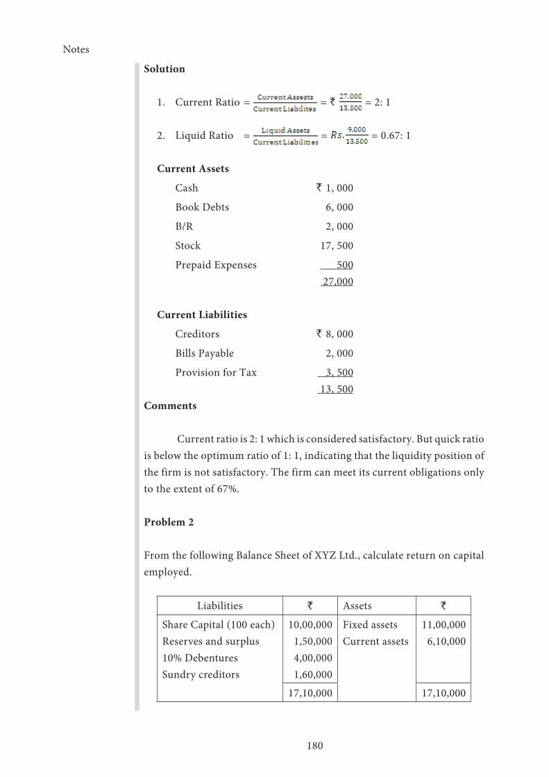
Notes

180

Solution

1. Current Ratio = = ` = 2: 1

2. Liquid Ratio = = = 0.67: 1

Current Assets

Cash ` 1, 000

Book Debts 6, 000

B/R 2, 000

Stock 17, 500

Prepaid Expenses 500 27,000

Current Liabilities

Creditors ` 8, 000

Bills Payable 2, 000

Provision for Tax 3, 500 13, 500

Comments

Current ratio is 2: 1 which is considered satisfactory. But quick ratio is below the optimum ratio of 1: 1, indicating that the liquidity position of the firm is not satisfactory. The firm can meet its current obligations only to the extent of 67%.

Problem 2

From the following Balance Sheet of XYZ Ltd., calculate return on capital employed.

Liabilities ` Assets `

Share Capital (100 each)Reserves and surplus10% DebenturesSundry creditors

10,00,000 1,50,000 4,00,000 1,60,000

Fixed assetsCurrent assets

11,00,000 6,10,000

17,10,000 17,10,000

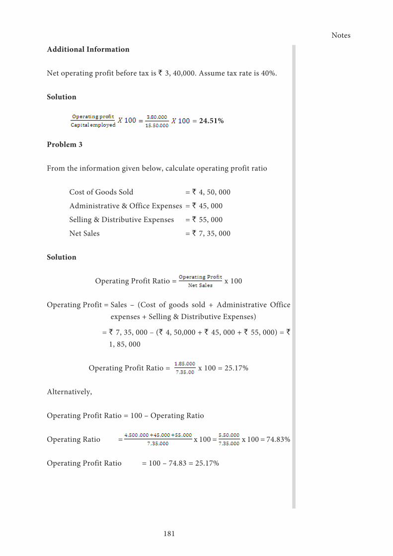
Notes

181

Additional Information

Net operating profit before tax is ` 3, 40,000. Assume tax rate is 40%.

Solution

= = 24.51%

Problem 3

From the information given below, calculate operating profit ratio

Cost of Goods Sold = ` 4, 50, 000

Administrative & Office Expenses = ` 45, 000

Selling & Distributive Expenses = ` 55, 000

Net Sales = ` 7, 35, 000

Solution

Operating Profit Ratio = x 100

Operating Profit = Sales – (Cost of goods sold + Administrative Office expenses + Selling & Distributive Expenses)

= ̀ 7, 35, 000 – (` 4, 50,000 + ` 45, 000 + ` 55, 000) = `

1, 85, 000

Operating Profit Ratio = x 100 = 25.17%

Alternatively,

Operating Profit Ratio = 100 – Operating Ratio

Operating Ratio = x 100 = x 100 = 74.83%

Operating Profit Ratio = 100 – 74.83 = 25.17%

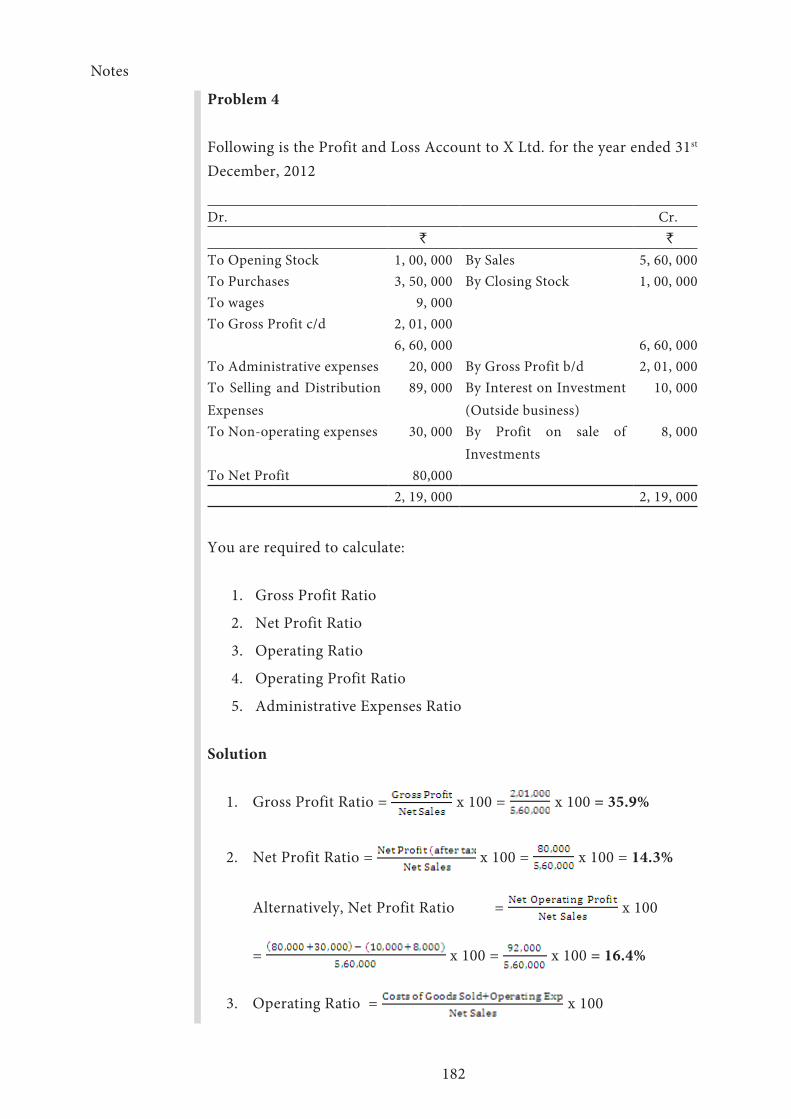
Notes

182

Problem 4

Following is the Profit and Loss Account to X Ltd. for the year ended 31st December, 2012

Dr. Cr.` `

To Opening Stock 1, 00, 000 By Sales 5, 60, 000To Purchases 3, 50, 000 By Closing Stock 1, 00, 000To wages 9, 000To Gross Profit c/d 2, 01, 000

6, 60, 000 6, 60, 000To Administrative expenses 20, 000 By Gross Profit b/d 2, 01, 000To Selling and Distribution Expenses

89, 000 By Interest on Investment (Outside business)

10, 000

To Non-operating expenses 30, 000 By Profit on sale of Investments

8, 000

To Net Profit 80,0002, 19, 000 2, 19, 000

You are required to calculate:

1. Gross Profit Ratio

2. Net Profit Ratio

3. Operating Ratio

4. Operating Profit Ratio

5. Administrative Expenses Ratio

Solution

1. Gross Profit Ratio = x 100 = x 100 = 35.9%

2. Net Profit Ratio = x 100 = x 100 = 14.3%

Alternatively, Net Profit Ratio = x 100

= x 100 = x 100 = 16.4%

3. Operating Ratio = x 100

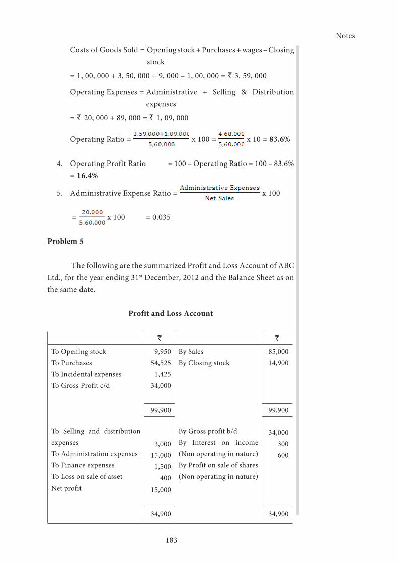
Notes

183

Costs of Goods Sold = Opening stock + Purchases + wages – Closing stock

= 1, 00, 000 + 3, 50, 000 + 9, 000 – 1, 00, 000 = ` 3, 59, 000

Operating Expenses = Administrative + Selling & Distribution expenses

= ` 20, 000 + 89, 000 = ` 1, 09, 000

Operating Ratio = x 100 = x 10 = 83.6%

4. Operating Profit Ratio = 100 – Operating Ratio = 100 – 83.6% = 16.4%

5. Administrative Expense Ratio = x 100

= x 100 = 0.035

Problem 5

The following are the summarized Profit and Loss Account of ABC Ltd., for the year ending 31st December, 2012 and the Balance Sheet as on the same date.

Profit and Loss Account

` `

To Opening stockTo PurchasesTo Incidental expensesTo Gross Profit c/d

To Selling and distribution expensesTo Administration expensesTo Finance expensesTo Loss on sale of assetNet profit

9,950 54,525

1,425 34,000

By SalesBy Closing stock

By Gross profit b/dBy Interest on income (Non operating in nature)By Profit on sale of shares (Non operating in nature)

85,000 14,900

99,900 99,900

3,00015,000 1,500

40015,000

34,000 300 600

34,900 34,900

Notes

184

Balance Sheet

Liabilities ` Assets `

2000 Equity shares of ` 10 eachReservesCurrent liabilitiesProfit and loss a/c

20,000 9,000

13,000 6,000

Land & BuildingPlant & MachineryStock in tradeSundry debtorsCash & Bank balance

15,000 8,000

14,900 7,100 3,000

48,000 48,000

Calculate

(i) Current ratio

(ii) Quick ratio

(iii) Operating ratio

(iv) Stock turnover ratio

(v) Fixed assets turnover ratio

Solution

a) Current ratio =

= = 1.92

b) Quick/Liquid/Acid Test Ratio =

Quick assets/Liquid assets = Current assets – (Stock and Prepaid expenses)

25,000 – 14,900 = 10,100 = = 0.77

c) Operating ratio = x 100

= x 100 = 83%

Notes

185

1. Stock turnover ratio = = = 4.1

2. Fixed Assets Turnover Ratio =

Fixed assets = Land & Building + Plant & Machinery

15,000 + 8,000 = 23,000 = = 3.69

****

Notes

186

Lesson 4.2 - Funds Flow Analysis

Meaning of Funds

The term ‘funds’ has several meanings. In a narrow sense, ‘funds’ means cash and a funds flow statement is prepared based upon this premise only. In a broader sense, ‘funds’ is considered to be equivalent to money. In a popular sense, a fund means working capital. The term working capital is defined as the excess of current assets over current liabilities.

Concepts of Working Capital

There are also two concepts of working capital—gross working capital and net working capital. Gross working capital refers to the total amount a firm invested in current assets while the term net working capital means excess of current assets over current liabilities

Meaning of Current Assets and Current Liabilities

Current assets refer to those assets which can be easily converted in to cash normally within a period of one year. While current liabilities are those liabilities which have to be paid in the ordinary course of time i.e. normally liabilities have to be settled within a period of one accounting year.

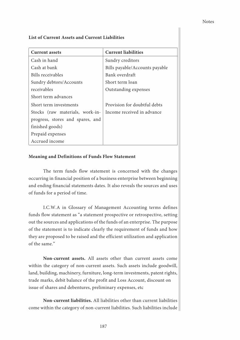
Notes

187

List of Current Assets and Current Liabilities

Current assets Current liabilities

Cash in handCash at bankBills receivablesSundry debtors/Accounts receivablesShort term advances

Sundry creditorsBills payable/Accounts payableBank overdraftShort term loanOutstanding expenses

Short term investmentsStocks (raw materials, work-in-progress, stores and spares, and finished goods)Prepaid expensesAccrued income

Provision for doubtful debtsIncome received in advance

Meaning and Definitions of Funds Flow Statement

The term funds flow statement is concerned with the changes occurring in financial position of a business enterprise between beginning and ending financial statements dates. It also reveals the sources and uses of funds for a period of time.

I.C.W.A in Glossary of Management Accounting terms defines funds flow statement as “a statement prospective or retrospective, setting out the sources and applications of the funds of an enterprise. The purpose of the statement is to indicate clearly the requirement of funds and how they are proposed to be raised and the efficient utilization and application of the same.”

Non-current assets. All assets other than current assets come within the category of non-current assets. Such assets include goodwill, land, building, machinery, furniture, long-term investments, patent rights, trade marks, debit balance of the profit and Loss Account, discount on issue of shares and debentures, preliminary expenses, etc

Non-current liabilities. All liabilities other than current liabilities come within the category of non-current liabilities. Such liabilities include

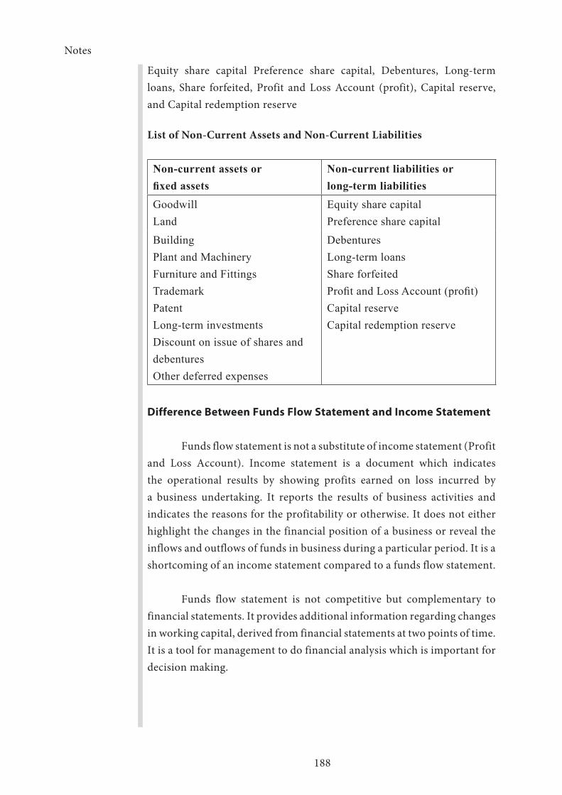
Notes

188

Equity share capital Preference share capital, Debentures, Long-term loans, Share forfeited, Profit and Loss Account (profit), Capital reserve, and Capital redemption reserve

List of Non-Current Assets and Non-Current Liabilities Non-current assets or fixed assets

Non-current liabilities or long-term liabilities

GoodwillLand

Equity share capitalPreference share capital

BuildingPlant and MachineryFurniture and FittingsTrademarkPatentLong-term investmentsDiscount on issue of shares and debenturesOther deferred expenses

DebenturesLong-term loansShare forfeitedProfit and Loss Account (profit)Capital reserveCapital redemption reserve

Difference Between Funds Flow Statement and Income Statement

Funds flow statement is not a substitute of income statement (Profit and Loss Account). Income statement is a document which indicates the operational results by showing profits earned on loss incurred by a business undertaking. It reports the results of business activities and indicates the reasons for the profitability or otherwise. It does not either highlight the changes in the financial position of a business or reveal the inflows and outflows of funds in business during a particular period. It is a shortcoming of an income statement compared to a funds flow statement.

Funds flow statement is not competitive but complementary to financial statements. It provides additional information regarding changes in working capital, derived from financial statements at two points of time. It is a tool for management to do financial analysis which is important for decision making.

Notes

189

Difference between Funds Flow Statement and Income Statement are as follows:

1. Funds flow statement highlights the changes in the financial position of a business and indicates the various means by which funds were obtained during particular period and the ways by which these funds were employed whereas income statement does not reveal the inflows and outflows of funds but depicts the items of expenses and income arrived at the figure of profit or loss.

2. Funds flow statement is complementary to income statement. It helps preparation of funds flow statement. Income statement is not prepared from funds flow statement.

3. While preparing funds flow statement, both capital and revenue items are considered, but for the preparation of income statement, only revenue items are taken into account.

4. There is no prescribed format for preparing a funds flow statement. But income statement is prepared in a prescribed format.

Difference Between Funds Flow Statement and Balance Sheet

A Balance sheet is a statement which reveals the financial position or status of a business on a given date. It is prepared at the end of the accounting period. Balance sheet contains various assets and liabilities of an undertaking. Funds flow statement tells us many financial facts which a Balance sheet fails to do so. Balance Sheet fails to disclose the causes for changes in the assets and liabilities between two different points of time. Again, while Balance Sheet is the end result of all the accounting operations for a period of time, funds flow statement is essentially a post Balance Sheet exercise. Funds statements are prepared to show the various sources from which the funds came into business and the various applications where they have been used.

The main difference between funds flow statement and balance Sheet are as follows:

1. Funds flow statement is a statement of changes in financial position and, hence, is dynamic in nature. But Balance Sheet is a statement of financial position on a particular date hence is static in nature.

Notes

190

2. Funds flow statement shows the sources and the uses of funds in a particular period of time, whereas Balance Sheet depicts the assets and liabilities at a particular point of time.

3. Funds flow statement is a tool of management for financial analysis, which helps making decisions, but income statement is not of much help to management in decision-making

4. Usually, a schedule of changes in working capital has to be prepared before preparing funds flow statement. But no such schedule of changes is required for the preparation of Balance Sheet. Preparation of balance sheet is preceded by preparation; Profit and Loss Account.

Uses and Importance of Funds Flow Statement

Funds flow statement helps a business enterprise in following ways.

1. In the Analysis of Financial Operations

The funds flow statement explains causes for changes and also the effect of such changes on the liquidity position of the company. Suppose a company may be having operating profit but still its cash position may be bad. The funds flow statement gives clear answers to this situation.

2. It Helps to the Formation of a Good Dividend Policy

Sometimes a firm may not be able to distribute the dividends to its equity shareholders for wanting of liquid cash despite the fact that the firm has made sufficient profits. The funds flow statement helps the firm in such a circumstance.

3. It Helps in the Proper Allocation of Resources

A projected funds flow statement helps the firm for the best deployment of the resources available with the firm.

Notes

191

4. It Acts as a Future Guide

A projected funds flow statement helps the company to identify the future needs of the funds and thereby the company can take necessary initiatives to arrange the funds.

5. It Helps in Determining Working Capital

A funds flow statement helps in explaining how efficiently the management has used its working capital and also suggests ways to improve the working capital position of the firm.

Limitations of Funds Flow Statement

1. Funds flow statement is not a substitute for financial statements; it provides some information regarding changes in working capital

2. It is historical in nature, so, its value is limited from the viewpoint of future operations.

3. This statement lacks originality, as it is only a rearrangement of data operating in the financial statements.

4. When a transaction affects either both current items or non-current items they are not recorded in the financial statement.

5. It is not generally considered as a sophisticated item for financial analysis.

Procedures for Preparing Funds Flow Statement

Funds flow statement is a method by which we study changes in the financial position of a business enterprise between beginning and ending financial statement dates.

Hence, the funds flow statement is prepared by comparing two Balance sheets and, with the help of such, other information derived from the accounts, as may be needed. The preparation of a funds flow statement consists of three steps

1. Schedule of changes in working capital which shows whether there is increase in working capital or decrease in working capital.

Notes

192

2. Funds from operation or adjusted profit and loss account which exhibits funds from operation

3. Funds flow statement reveals the sources and uses of funds

The preparation of Statement of Schedule of Changes in Working Capital is as follows.

The statement of schedule of changes in working capital deals with the current assets and current liabilities alone, as they are shown in the Balance Sheets of the current and the previous years. All non-current assets and non-current liabilities, and profits and losses ignore additional information available. Each current asset and current liability in the period’s Balance sheet is compared with that shown in the previous period’s Balance Sheet. Increase or decrease in each of the assets and liabilities is noted. The effect of such increase or decrease during the period in each item is recorded individually on the working capital. Finally, the overall change in the working capital is calculated. It is possible that working capital might have increase or decrease as the final result.

The following interpretations have to be taken into consideration when schedule of changes in working capital is prepared.

1. An increase in current assets and decrease in current liabilities will result in increase in working capital.

2. A decrease in current assets and increase in current liabilities will result in decrease in working capital.

Preparation of Schedule of changes in working capital

Current Assets 20xx 20xx Increase Decrease

Cash in hand xxx xxx xxx -

Cash at bank xxx xxx xxx -

Bills receivable xxx xxx - xxx

Debtors. xxx xxx - xxx

Stock. investment xxx xxx xxx -

Prepaid expense xxx xxx xxx -

Other current assets xxx xxx

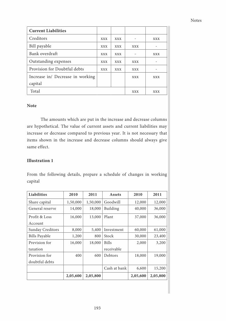
Notes

193

Current Liabilities

Creditors xxx xxx - xxx

Bill payable xxx xxx xxx -

Bank overdraft xxx xxx - xxx

Outstanding expenses xxx xxx xxx -

Provision for Doubtful debts xxx xxx xxx -

Increase in/ Decrease in working capital

xxx xxx

Total xxx xxx

Note

The amounts which are put in the increase and decrease columns are hypothetical. The value of current assets and current liabilities may increase or decrease compared to previous year. It is not necessary that items shown in the increase and decrease columns should always give same effect.

Illustration 1

From the following details, prepare a schedule of changes in working capital

Liabilities 2010 2011 Assets 2010 2011

Share capital 1,50,000 1,50,000 Goodwill 12,000 12,000General reserve 14,000 18,000 Building 40,000 36,000

Profit & Loss Account

16,000 13,000 Plant 37,000 36,000

Sunday Creditors 8,000 5,400 Investment 60,000 61,000Bills Payable 1,200 800 Stock 30,000 23,400Prevision for taxation

16,000 18,000 Bills receivable

2,000 3,200

Provision for doubtful debts

400 600 Debtors 18,000 19,000

Cash at bank 6,600 15,200

2,05,600 2,05,800 2,05,600 2,05,800

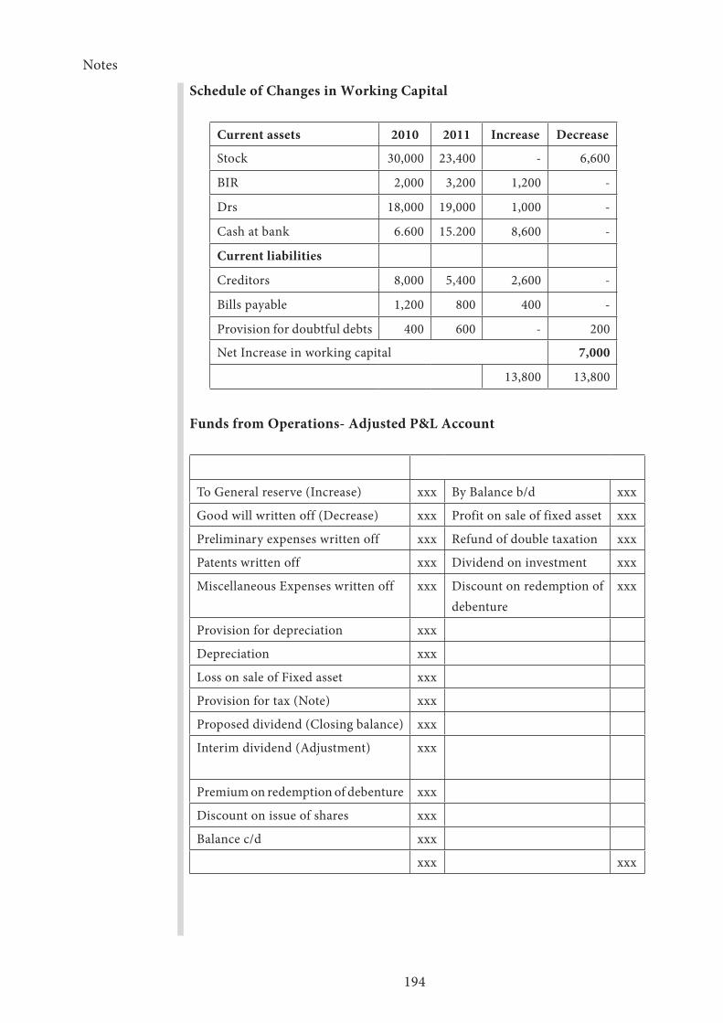
Notes

194

Schedule of Changes in Working Capital

Current assets 2010 2011 Increase Decrease

Stock 30,000 23,400 - 6,600

BIR 2,000 3,200 1,200 -

Drs 18,000 19,000 1,000 -

Cash at bank 6.600 15.200 8,600 -

Current liabilities

Creditors 8,000 5,400 2,600 -

Bills payable 1,200 800 400 -

Provision for doubtful debts 400 600 - 200

Net Increase in working capital 7,000

13,800 13,800

Funds from Operations- Adjusted P&L Account

To General reserve (Increase) xxx By Balance b/d xxx

Good will written off (Decrease) xxx Profit on sale of fixed asset xxx

Preliminary expenses written off xxx Refund of double taxation xxx

Patents written off xxx Dividend on investment xxx

Miscellaneous Expenses written off xxx Discount on redemption of debenture

xxx

Provision for depreciation xxx

Depreciation xxx

Loss on sale of Fixed asset xxx

Provision for tax (Note) xxx

Proposed dividend (Closing balance) xxx

Interim dividend (Adjustment) xxx

Premium on redemption of debenture xxx

Discount on issue of shares xxx

Balance c/d xxx

xxx xxx

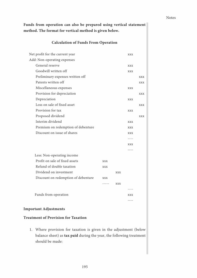
Notes

195

Funds from operation can also be prepared using vertical statement method. The format for vertical method is given below.

Calculation of Funds From Operation

Net profit for the current year xxxAdd: Non-operating expenses

General reserve xxx Goodwill written off xxx Preliminary expenses written off xxx Patents written off xxx Miscellaneous expenses xxx Provision for depreciation xxx Depreciation xxx Loss on sale of fixed asset xxx Provision for tax xxx Proposed dividend xxx Interim dividend xxx Premium on redemption of debenture xxx Discount on issue of shares xxx ---- xxx ----Less: Non-operating income Profit on sale of fixed assets xxx Refund of double taxation xxx Dividend on investment xxx Discount on redemption of debenture xxx ----- xxx ----Funds from operation xxx

----

Important Adjustments

Treatment of Provision for Taxation

1. Where provision for taxation is given in the adjustment (below balance sheet) as tax paid during the year, the following treatment should be made:

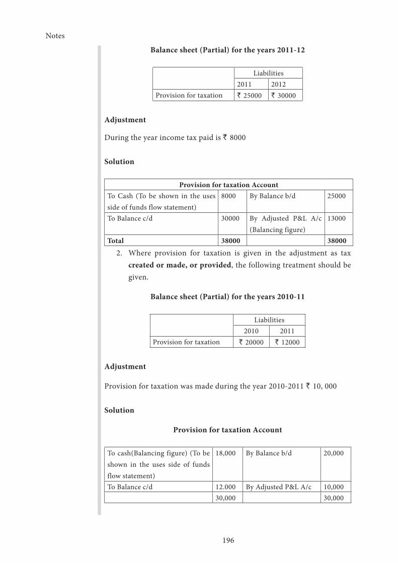
Notes

196

Balance sheet (Partial) for the years 2011-12

Liabilities2011 2012

Provision for taxation ` 25000 ` 30000

Adjustment

During the year income tax paid is ` 8000

Solution

Provision for taxation AccountTo Cash (To be shown in the uses side of funds flow statement)

8000 By Balance b/d 25000

To Balance c/d 30000 By Adjusted P&L A/c (Balancing figure)

13000

Total 38000 38000

2. Where provision for taxation is given in the adjustment as tax created or made, or provided, the following treatment should be given.

Balance sheet (Partial) for the years 2010-11

Liabilities2010 2011

Provision for taxation ` 20000 ` 12000

Adjustment

Provision for taxation was made during the year 2010-2011 ` 10, 000

Solution

Provision for taxation Account

To cash(Balancing figure) (To be shown in the uses side of funds flow statement)

18,000 By Balance b/d 20,000

To Balance c/d 12.000 By Adjusted P&L A/c 10,00030,000 30,000

Notes

197

Treatment of Depreciation

Fixed Asset Account

To Balance b/d xxx By Adjusted P&L A/c (Depreciation)

xxx

To Adjusted P&L A/c (Profit on sale of fixed asset)

xxx By Adjusted P&L A/c (Loss on sale of fixed asset)

To Cash (Purchase)( Balancing figure)

xxx By Cash (Sales)(Balancing figure)

xxx

By Balance c/d xxxTotal xxx xxx

Treatment No.1

Balance Sheet (Partial) for the years 2009-10

Assets side 2009 2010

Land & Building ` 2,00,000 ` 1,70,000

Adjustment

Depreciation of ` 20000 has been changed on land and Building in 2010

Solution

Land and Building Account

To Balance b/d 2,00,000 By Adjusted P&L A/c (Depreciation) 20,000

Cash (Sales)(Balancing figure) 10,000

By Balance c/d 1,70,000

Total 2,00,000 2,00,000

Treatment No.2

Balance Sheet (Partial) for the years 2010-11

Asset side 2010 2011

Plant & Machinery ` 60,000 ` 1,00,000

Adjustment: Plant costing ` 20.000/. (Accumulated depreciation of `

12000) was sold for ` 6000/-

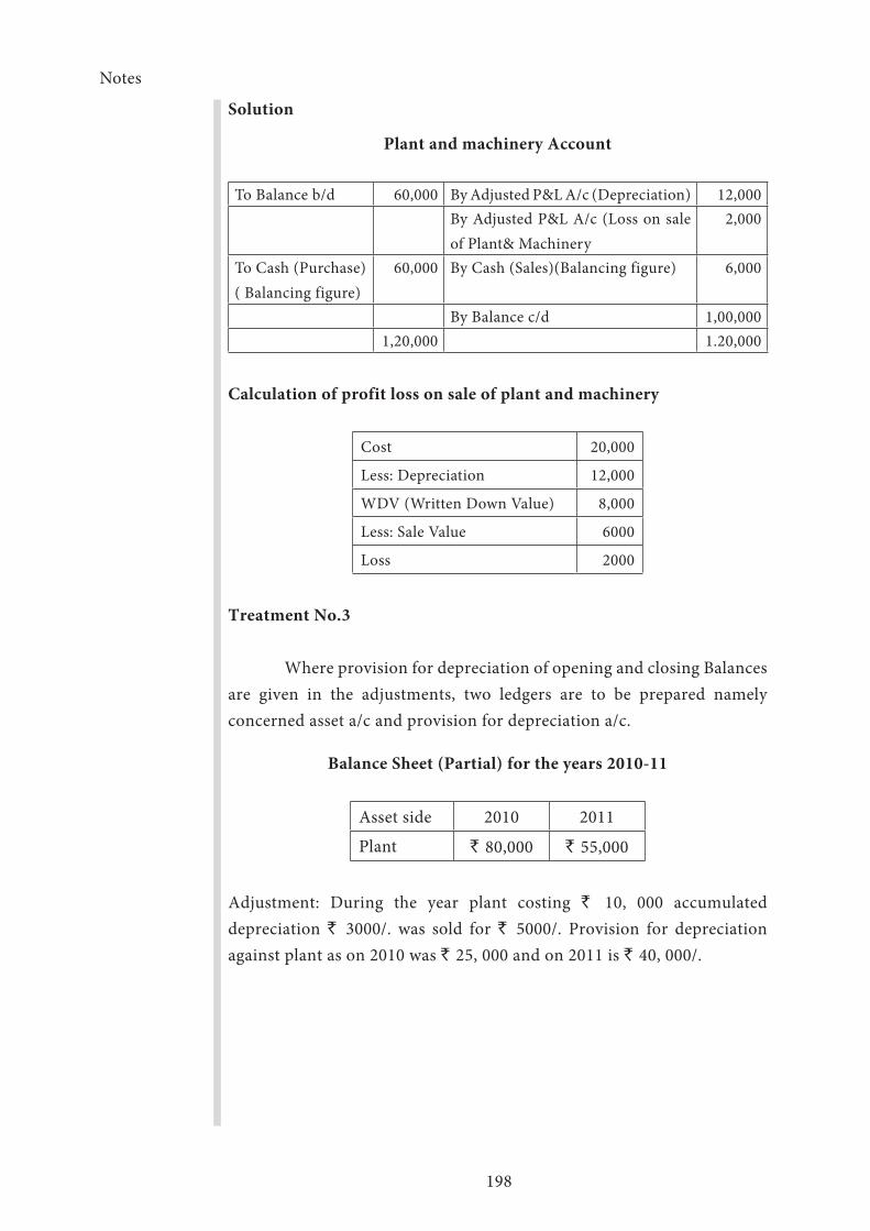
Notes

198

Solution

Plant and machinery Account

To Balance b/d 60,000 By Adjusted P&L A/c (Depreciation) 12,000By Adjusted P&L A/c (Loss on sale of Plant& Machinery

2,000

To Cash (Purchase)( Balancing figure)

60,000 By Cash (Sales)(Balancing figure) 6,000

By Balance c/d 1,00,0001,20,000 1.20,000

Calculation of profit loss on sale of plant and machinery

Cost 20,000

Less: Depreciation 12,000

WDV (Written Down Value) 8,000

Less: Sale Value 6000

Loss 2000

Treatment No.3

Where provision for depreciation of opening and closing Balances are given in the adjustments, two ledgers are to be prepared namely concerned asset a/c and provision for depreciation a/c.

Balance Sheet (Partial) for the years 2010-11

Asset side 2010 2011

Plant ` 80,000 ` 55,000

Adjustment: During the year plant costing ` 10, 000 accumulated depreciation ` 3000/. was sold for ` 5000/. Provision for depreciation against plant as on 2010 was ` 25, 000 and on 2011 is ` 40, 000/.

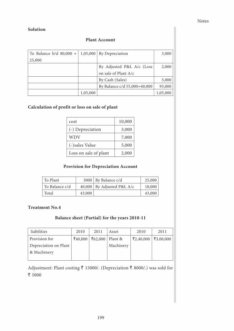
Notes

199

Solution

Plant Account

To Balance b/d 80,000 + 25,000

1,05,000 By Depreciation 3,000

By Adjusted P&L A/c (Loss on sale of Plant A/c

2,000

By Cash (Sales) 5,000By Balance c/d 55,000+40,000 95,000

1,05,000 1,05,000

Calculation of profit or loss on sale of plant

cost 10,000

(-) Depreciation 3,000

WDV 7,000

(-)sales Value 5,000

Loss on sale of plant 2,000

Provision for Depreciation Account

To Plant 3000 By Balance c/d 25,000To Balance c/d 40,000 By Adjusted P&L A/c 18,000Total 43,000 43,000

Treatment No.4

Balance sheet (Partial) for the years 2010-11

liabilities 2010 2011 Asset 2010 2011

Provision for Depreciation on Plant & Machinery

`40,000 `62,000 Plant & Machinery

`2,40,000 `3,00,000

Adjustment: Plant costing ` 15000/. (Depreciation ` 8000/.) was sold for ` 5000

Notes

200

Solution

Plant & Machinery Account

To Balance b/d 2,40,000 By Depreciation 8,000

By Adjusted P&L A/c (Loss on sale of Plant & Machinery A/c

2,000

To Cash (purchase)(Balancing Figure)

75,000 By Cash (Sales) 5000

By Balance c/d 3,00,000

3,15.000 315000

Calculation of profit or loss on sale of plant and machinery

Cost 15,000(-) Depreciation 8000WDV 7,000(-) Sales Value 5,000Loss 2,000

Provision for Depreciation Account

To Machinery 8,000 By Balance B/D 40,000

To Balance C/D 62,000 By Adjusted P&L A/c (Balancing figure)

30,000

Total 70,000 70.000

From the following particulars, calculate funds from operations. Profit &Loss Account

To Salaries ` 5,000 By Gross profit ` 50,000To Rent 3,000 By Profit on sale of Building

Book value ` 10000 Sold for ` 15000

5,000To Depreciation on plant 5,000

To Printing & stationery 3,000 To Preliminary express written off

2,000

To Goodwill written off 3,000To provision for tax 4,000

Notes

201

To Proposed dividends 6,000To Net profit taken to Balance sheet

24,000

Total 55,000 55,000

Calculation of funds from operation under vertical method.

Net profit ` 24, 000

Add: Non-operating expenses

Depreciation on Plant 5,000

Preliminary expenses 2,000

Goodwill written off 3,000

Provision for tax 4,000

Proposed dividend 6,000 ______ 44,000

Less: Non-operating expenses

Profit on sale of Building 5,000 ______Funds from operation 39,000 ______

Calculation of funds from operation under T form method

Funds from operation

-Adjusted Profit & Loss Account

To Depreciation on Plant 5,000 By Balance b/d -To Preliminary expenses 2,000 By Profit on sale of Building 5,000To Goodwill written off 3,000To Provision for tax 4,000 By Funds from operation

(Balancing figure)39,000

Proposed dividend 6,000

To Balance c/d 24,000 44,000

Notes

202

Format of Funds Flow Statement

Sources Application

Issue of share capital xxx Redemption of share capital xxxIssue of debentures xxx Redemption of debentures xxxBorrowing from Bank xxx Repayment of Bank loan xxxIssue of share Premium xxx Purchase of fixed asset xxxSale of Investment xxx Purchase of Investment xxxSale of Fixed Asset xxx Increase in working capital xxxDecrease in Working Capital xxx Provision for Taxation xxx Funds from operation xxx Proposed dividend xxx (opening Balance)Dividend on investment xxx interim dividen(adjustment) xxxDrawings (Note) xxx ----- ---- xxx xxx

----- -----

Comprehensive Funds Flow Statments

1. From the following balance sheets of X Ltd. On 31st December, 2011 and 2012, you are required to prepare.

a) A schedule of changes in working capital.

b) A Funds flow Statement.

Liabilities2011

`

2012`

Assets2011

`

2012`

Share CapitalGeneral ReserveProfit & Loss A/cSundry CreditorsBills PayableProvision for TaxationProvision for Doubtful Debts

1,10,000 14,000 16,000

8,000 1,200

16,000 400

1,10,00018,00013,000

5,400800

18,000600

GoodwillBuildingPlantInvestmentStocksBills ReceivableDebtorsCash at Bank

22,00040,00037,00010,00030,000

2,000

18,0006,600

22,00036,00036,00011,00023,400

3,200

19,00015,200

1,65,600 1,65,800 1,65,600 1,65,800

Notes

203

The following additional information has also been given:

1) Depreciation charged on Plant was ` 4,000 and on Building ` 4,000

2) Provision for taxation of ` 19,000 was made during the year 2012.

3) Interim Dividend of ` 18, 000 was paid during the year 2012.

Solution

Schedule of Changes in Working Capital

Particulars2011

`

2012`

Increase`

Decrease`

Current Assets:Cas at BankDebtorsBills ReceivableStockCurrent Liabilities:Provision for Doubtful DebtsBills PayableSundry CreditorsNet Increase in Working Capital

6,60018,000

2,00030,000

4001,2008,000

15,20019,000

3,20023,400

600800

5,400

Total

8,6001,0001,200

4002,600

13,800

6,600200

-

7,000

13,800

Plant Account

To Balance b/d 37,000 By Adjusted P&L A/c 4,000To Cash (purchase) (B/F) 3,000 By balance c/d 36,000

40,000 40,000

Building Account

To Balance b/d 40,000 By Adjusted P&L A/c 4,000By Balance c/d 36,000

40,000 40,000

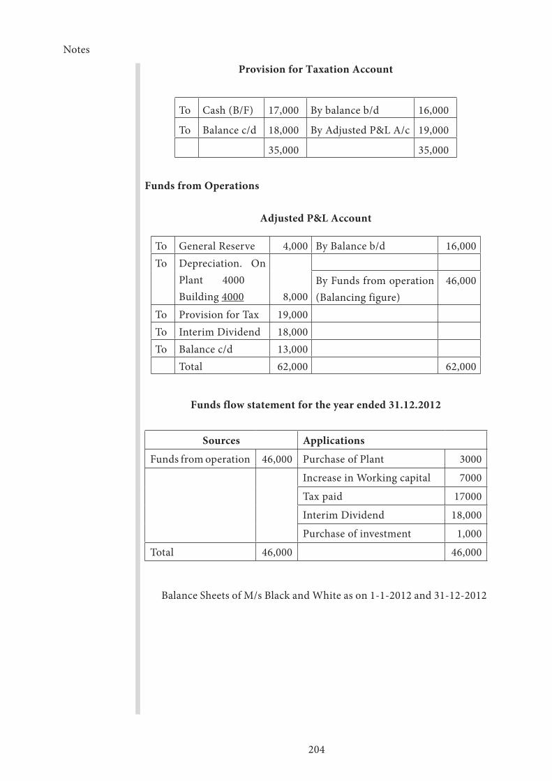
Notes

204

Provision for Taxation Account

To Cash (B/F) 17,000 By balance b/d 16,000

To Balance c/d 18,000 By Adjusted P&L A/c 19,000

35,000 35,000

Funds from Operations

Adjusted P&L Account

To General Reserve 4,000 By Balance b/d 16,000To Depreciation. On

Plant 4000Building 4000 8,000

By Funds from operation (Balancing figure)

46,000

To Provision for Tax 19,000To Interim Dividend 18,000To Balance c/d 13,000

Total 62,000 62,000

Funds flow statement for the year ended 31.12.2012

Sources Applications

Funds from operation 46,000 Purchase of Plant 3000

Increase in Working capital 7000

Tax paid 17000

Interim Dividend 18,000

Purchase of investment 1,000

Total 46,000 46,000

Balance Sheets of M/s Black and White as on 1-1-2012 and 31-12-2012

205

Balance Sheet

Liabilities1-1-12

`

31-12-12`

Assets1-1-2012

`

31-12-12`

CreditorsMr. White’s LoanLoan from P.N. BankCapital

40,000 25,000 40,000

1,25,000

44,000 -

50,0001,53,000

CashDebtorsStockMachineryLandBuilding

10,00030,00035,00080,00040,00035,000

7,00050,00025,00055,00050,00060,000

2,30,000 2,47,000 2,30,000 2,47,000

During the year machine costing ` 10, 000 (accumulated depreciation ` 3, 000) was sold for ` 5, 000. The provision for Depreciation against machinery as on 1-1-2012 was ` 25, 000 and on 31-12-2012 ` 40, 000. Net Profit for the year 2012 amounted to ` 45, 000. You are required to prepare Funds (Working capital) Flow Statement.

Note

Where net profit/drawing is given in the adjustment like above, a separate capital account shall be prepared to find out hidden information i.e. drawing/net profit.

Capital Account

To Drawings (B/F) xxx By Balance b/d xxx

To Balance c/d xxx By Net Profit (Balancing figure) xxx

Total xxx xxx

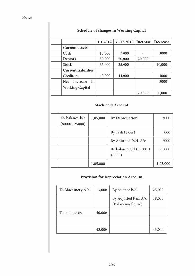
Notes

206

Schedule of changes in Working Capital

1.1.2012 31.12.2012 Increase DecreaseCurrent assetsCash 10,000 7000 - 3000Debtors 30,000 50,000 20,000 -Stock 35,000 25,000 - 10,000Current liabilitiesCreditors 40,000 44,000 4000Net Increase in Working Capital

3000

20,000 20,000

Machinery Account

To balance b/d (80000+25000)

1,05,000 By Depreciation 3000

By cash (Sales) 5000

By Adjusted P&L A/c 2000

By balance c/d (55000 + 40000)

95,000

1,05,000 1,05,000

Provision for Depreciation Account

To Machinery A/c 3,000 By balance b/d 25,000

By Adjusted P&L A/c (Balancing figure)

18,000

To balance c/d 40,000

43,000 43,000

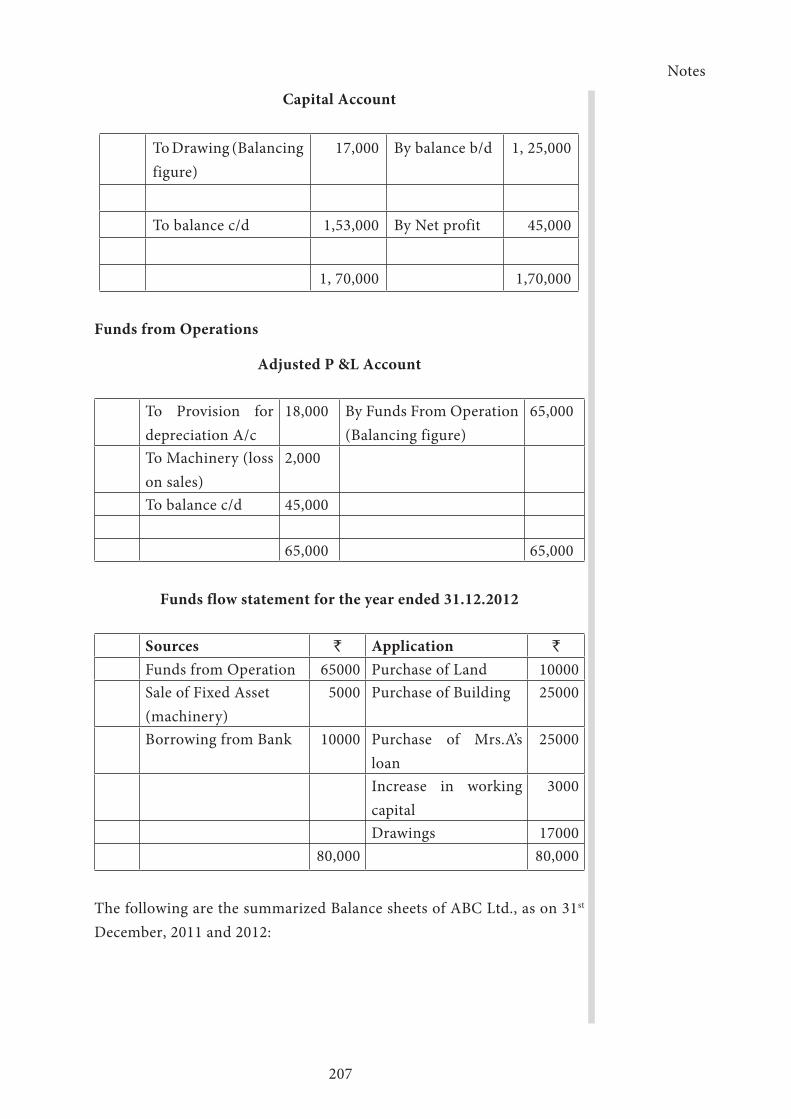
Notes

207

Capital Account

To Drawing (Balancing figure)

17,000 By balance b/d 1, 25,000

To balance c/d 1,53,000 By Net profit 45,000

1, 70,000 1,70,000

Funds from Operations

Adjusted P &L Account

To Provision for depreciation A/c

18,000 By Funds From Operation (Balancing figure)

65,000

To Machinery (loss on sales)

2,000

To balance c/d 45,000

65,000 65,000

Funds flow statement for the year ended 31.12.2012

Sources ` Application `Funds from Operation 65000 Purchase of Land 10000Sale of Fixed Asset (machinery)

5000 Purchase of Building 25000

Borrowing from Bank 10000 Purchase of Mrs.A’s loan

25000

Increase in working capital

3000

Drawings 1700080,000 80,000

The following are the summarized Balance sheets of ABC Ltd., as on 31st December, 2011 and 2012:

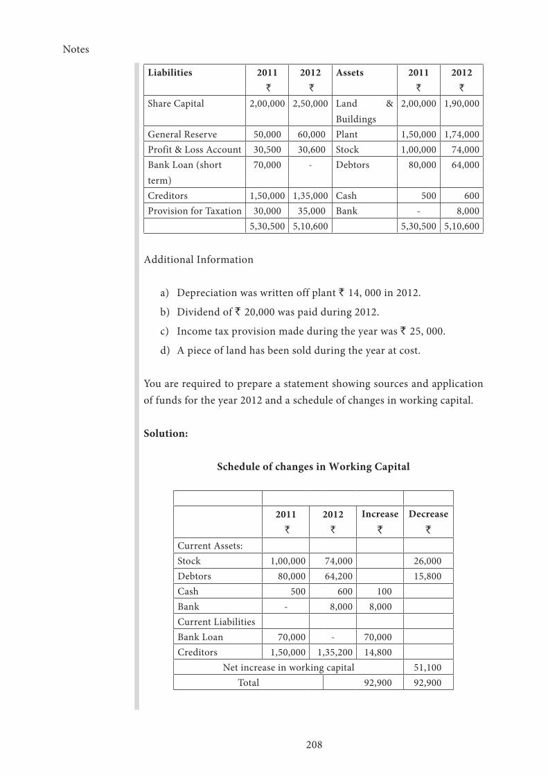
Notes

208

Liabilities 2011 `

2012 `

Assets 2011`

2012`

Share Capital 2,00,000 2,50,000 Land & Buildings

2,00,000 1,90,000

General Reserve 50,000 60,000 Plant 1,50,000 1,74,000Profit & Loss Account 30,500 30,600 Stock 1,00,000 74,000Bank Loan (short term)

70,000 - Debtors 80,000 64,000

Creditors 1,50,000 1,35,000 Cash 500 600Provision for Taxation 30,000 35,000 Bank - 8,000

5,30,500 5,10,600 5,30,500 5,10,600

Additional Information

a) Depreciation was written off plant ` 14, 000 in 2012.

b) Dividend of ` 20,000 was paid during 2012.

c) Income tax provision made during the year was ` 25, 000.

d) A piece of land has been sold during the year at cost.

You are required to prepare a statement showing sources and application of funds for the year 2012 and a schedule of changes in working capital.

Solution:

Schedule of changes in Working Capital

2011 `

2012`

Increase `

Decrease `

Current Assets: Stock 1,00,000 74,000 26,000Debtors 80,000 64,200 15,800Cash 500 600 100Bank - 8,000 8,000Current Liabilities Bank Loan 70,000 - 70,000Creditors 1,50,000 1,35,200 14,800

Net increase in working capital 51,100Total 92,900 92,900

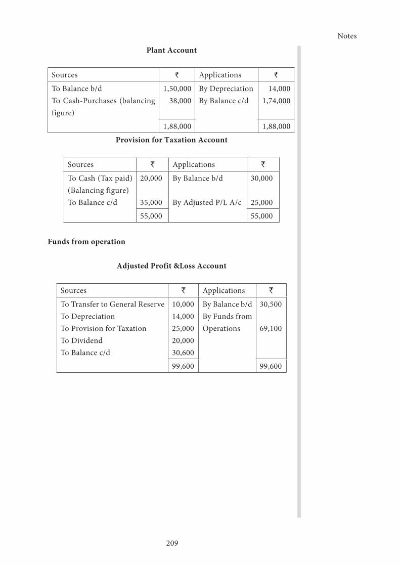
Notes

209

Plant Account

Sources ` Applications `

To Balance b/dTo Cash-Purchases (balancing figure)

1,50,000 38,000

By DepreciationBy Balance c/d

14,0001,74,000

1,88,000 1,88,000

Provision for Taxation Account

Sources ` Applications `

To Cash (Tax paid) (Balancing figure)To Balance c/d

20,000

35,000

By Balance b/d

By Adjusted P/L A/c

30,000

25,000

55,000 55,000

Funds from operation

Adjusted Profit &Loss Account

Sources ` Applications `

To Transfer to General Reserve To DepreciationTo Provision for TaxationTo Dividend To Balance c/d

10,00014,00025,00020,00030,600

By Balance b/dBy Funds from Operations

30,500 69,100

99,600 99,600

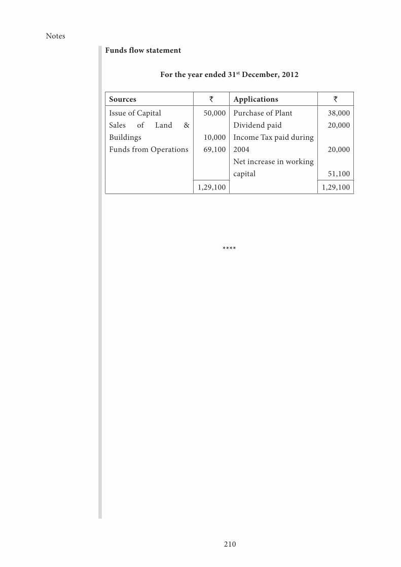
Notes

210

Funds flow statement

For the year ended 31st December, 2012

Sources ` Applications `

Issue of CapitalSales of Land & BuildingsFunds from Operations

50,000

10,00069,100

Purchase of PlantDividend paidIncome Tax paid during 2004Net increase in working capital

38,00020,000

20,000

51,100

1,29,100 1,29,100

****

Notes

211

Lesson 4.3 - Cash Flow Analysis

Introduction

Cash flow analysis is another important technique of financial analysis. It involves preparation of Cash Flow Statement for identifying sources and applications of cash; Cash flow statement may be prepared on the basis of actual or estimated data.

In the latter case, it is termed as ‘Projected Cash Flow Statement’, which is synonymous with the term ‘Cash Budget’. In the following pages we shall explain in detail in preparation of cash flow statement, utility and limitations of cash flow analysis etc.

Meaning of Cash Flow Statement

A Cash Flow Statement is a statement depicting change in cash position from one period to another. For example, if the cash balance of a business is shown by its Balance Sheet on 31st December, 1998 at ` 20,000 while the cash balance as per its Balance Sheet on 31st December, 1999 is ` 30,000, there has been an inflow of cash of ` 10,000 in the year 1999. The cash flow statement explains the reasons for such inflows or outflows of cash, as the case may be. It also helps management in making plans for the immediate future.

A Projected Cash Flow Statement or a Cash Budget will help the management in ascertaining how much cash will be available to meet obligations to trade creditors, to pay bank loans and to pay dividend to the shareholders. A proper planning of the cash resources will enable the management to have cash available whenever needed and put it to some profitable or productive use in case there is surplus cash available.

The term “Cash” here stands for cash and bank balances. In a narrower sense, funds are also used to denote cash. In such a case, the term “Funds” will exclude from its purview all other current assets and

Notes

212

current liabilities and the terms “Funds Flow Statement” and “Cash Flow Statement” will have synonymous meanings.

However, for the purpose of this study we are calling this part of study Cash Flow Analysis and not Funds Flow analysis.

Preparation of Cash Flow Statement

Cash Flow Statement can be prepared on the same pattern on which a Funds Flow Statement is prepared. The change in the cash position from one period to another is computed by taking into account “Sources” and” Applications” of cash.

Sources of Cash

Sources of cash can be both internal as well as external:

Internal Sources- Cash from operations is the main internal source. The Net Profit shown by the Profit and Loss Account will have to be adjusted for non-cash items for finding out cash from operations. Some of these items are as follows:

i) Depreciation. Depreciation does not result in outflow of cash and, therefore, net profit will have to be increased by the amount of depreciation or development rebate charged, in order to find out the real cash generated from operations.

(ii) Amortization of Intangible Assets. Goodwill, preliminary expenses, etc., when written off against profits, reduce the net profits without affecting the cash balance. The amounts written off should, therefore, be added back to profits to find out the cash from operations.

iii) Loss on Sale of Fixed Assets. It does not result in outflow of cash and, therefore, should be added back to profits.

iv) Gains from Sale of Fixed Assets. Since sale of fixed assets is taken as a separate source of cash, it should be deducted from net profits.

v) Creation of Reserves. If profit for the year has been arrived at after charging transfers to reserves, such transfers should be added back

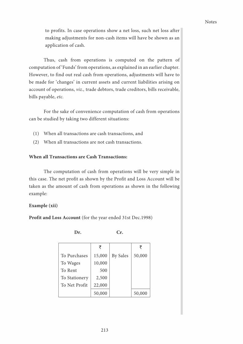
Notes

213

to profits. In case operations show a net loss, such net loss after making adjustments for non-cash items will have be shown as an application of cash.

Thus, cash from operations is computed on the pattern of computation of ‘Funds’ from operations, as explained in an earlier chapter. However, to find out real cash from operations, adjustments will have to be made for ‘changes’ in current assets and current liabilities arising on account of operations, viz., trade debtors, trade creditors, bills receivable, bills payable, etc.

For the sake of convenience computation of cash from operations can be studied by taking two different situations:

(1) When all transactions are cash transactions, and

(2) When all transactions are not cash transactions.

When all Transactions are Cash Transactions:

The computation of cash from operations will be very simple in this case. The net profit as shown by the Profit and Loss Account will be taken as the amount of cash from operations as shown in the following example:

Example (xii)

Profit and Loss Account (for the year ended 31st Dec.1998)

Dr. Cr.

` `

To PurchasesTo WagesTo RentTo StationeryTo Net Profit

15,00010,000

5002,500

22,000

By Sales 50,000

50,000 50,000

Notes

214

In the example given above, if all transactions are cash transactions, i.e., all purchases’ and expenses have been paid for in cash and all sales have been realized in cash, the cash from operations will be ` 22,000. i.e., the net profit shown in the Profit and Loss Account. Thus, in case of all transactions being cash transactions, the equation for computing cash from operations can be made out as follows:

Cash for Operations = Net Profit

When all Transactions are not Cash Transactions

In the example given above, we have computed cash from operations on the basis that all transactions are cash transactions. Because the business sells goods on credit, it purchases goods on credit.

Certain expenses are always outstanding and some of the incomes are not immediately realized. Under such circumstances, the net profit made by a firm cannot generate equivalent amount of cash. The computation of cash from operations in such a situation can be done conveniently if it is done in two stages:

(i) Computation of funds (i.e., working capital) from operations.

(ii) Adjustments in the funds so calculated for changes in the current assets (excluding cash) and current liabilities.

An illustration for computing ‘Funds’ from operations is given below. However, since there are no credit transactions, hence the amount of ‘Funds’ from operations is as a matter of fact, cash from operations as shown below:

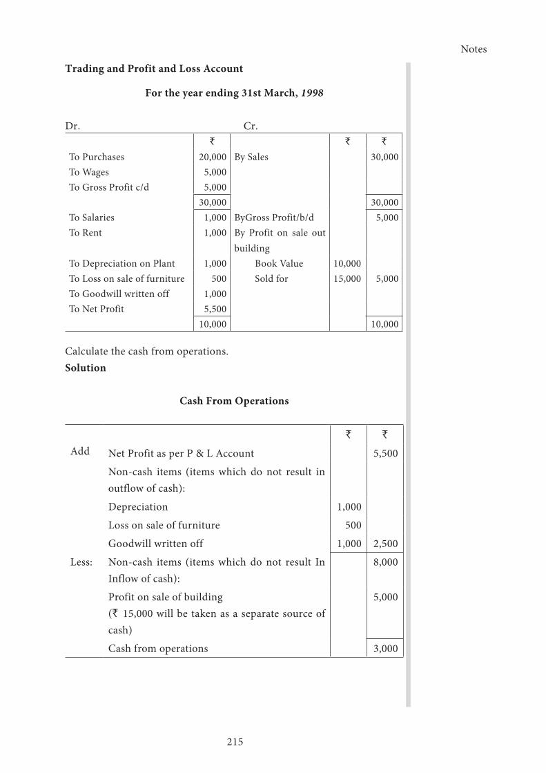
Notes

215

Trading and Profit and Loss Account

For the year ending 31st March, 1998

Dr. Cr.` ` `

To Purchases 20,000 By Sales 30,000To Wages 5,000To Gross Profit c/d 5,000

30,000 30,000To Salaries 1,000 ByGross Profit/b/d 5,000To Rent 1,000 By Profit on sale out

buildingTo Depreciation on Plant 1,000 Book Value 10,000To Loss on sale of furniture 500 Sold for 15,000 5,000To Goodwill written off 1,000To Net Profit 5,500

10,000 10,000

Calculate the cash from operations.Solution

Cash From Operations

Add

` `

Net Profit as per P & L Account 5,500

Non-cash items (items which do not result in outflow of cash):

Depreciation 1,000

Loss on sale of furniture 500

Goodwill written off 1,000 2,500

Less: Non-cash items (items which do not result In Inflow of cash):

8,000

Profit on sale of building(` 15,000 will be taken as a separate source of cash)

5,000

Cash from operations 3,000

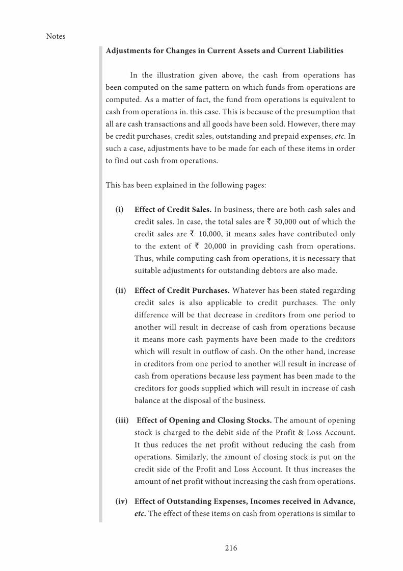
Notes

216

Adjustments for Changes in Current Assets and Current Liabilities

In the illustration given above, the cash from operations has been computed on the same pattern on which funds from operations are computed. As a matter of fact, the fund from operations is equivalent to cash from operations in. this case. This is because of the presumption that all are cash transactions and all goods have been sold. However, there may be credit purchases, credit sales, outstanding and prepaid expenses, etc. In such a case, adjustments have to be made for each of these items in order to find out cash from operations.

This has been explained in the following pages:

(i) Effect of Credit Sales. In business, there are both cash sales and credit sales. In case, the total sales are ` 30,000 out of which the credit sales are ` 10,000, it means sales have contributed only to the extent of ` 20,000 in providing cash from operations. Thus, while computing cash from operations, it is necessary that suitable adjustments for outstanding debtors are also made.

(ii) Effect of Credit Purchases. Whatever has been stated regarding credit sales is also applicable to credit purchases. The only difference will be that decrease in creditors from one period to another will result in decrease of cash from operations because it means more cash payments have been made to the creditors which will result in outflow of cash. On the other hand, increase in creditors from one period to another will result in increase of cash from operations because less payment has been made to the creditors for goods supplied which will result in increase of cash balance at the disposal of the business.

(iii) Effect of Opening and Closing Stocks. The amount of opening stock is charged to the debit side of the Profit & Loss Account. It thus reduces the net profit without reducing the cash from operations. Similarly, the amount of closing stock is put on the credit side of the Profit and Loss Account. It thus increases the amount of net profit without increasing the cash from operations.

(iv) Effect of Outstanding Expenses, Incomes received in Advance, etc. The effect of these items on cash from operations is similar to

Notes

217

the effect of creditors. This means any increase in these items will result in increase in cash from operations while any decrease means decrease in cash from operations. This is because net profit from operations is computed after charging to it all expenses whether paid or outstanding. In case certain expenses have not been paid, this will result in decrease of net profit without a corresponding decrease in cash from operations. Similarly, income received in advance is not taken into account while calculating profit from operations, since it relates to the next year. It, therefore, means cash from operations will be higher than the actual net profit as shown by the Profit and Loss Account. Consider the following example:

Example (xiii)

Net Profit for the year 1998 10,000Expenses outstanding as on 1.1.1998 2,000Expenses outstanding as on 31.12.1998 3,000Interest received in advance 1.1.1998 1,000Interest received in advance 31.12.1998 2,000The Cash from Operations will be computed as follows:Net Profit for the year 10,000Add: Expenses outstanding on 31.12.1998 3,000 Income received in advance on 31.12.1998 2,000 15,000

Less: Expenses outstanding on 1.1.1998 2,000 Interest received in advance on 1.1.1998 1,000 3,000Cash from Operations 12,000

Alternatively, Cash from Operations can be computed as follows:

Net profit for the year 10,000Add: Increase in Outstanding Expenses 1,000Add: Increase in Interest received in Advance 1,000 Cash from Operations 12,000

Thus, the effect of income received in advance and outstanding expenses on cash from operations can be shown as follows:

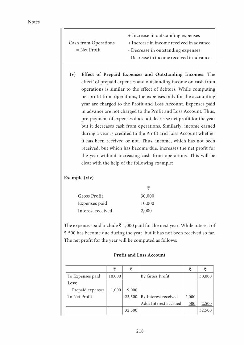
Notes

218

+ Increase in outstanding expenses + Increase in income received in advanceCash from Operations

- Decrease in outstanding expenses = Net Profit - Decrease in income received in advance

(v) Effect of Prepaid Expenses and Outstanding Incomes. The effect’ of prepaid expenses and outstanding income on cash from operations is similar to the effect of debtors. While computing net profit from operations, the expenses only for the accounting year are charged to the Profit and Loss Account. Expenses paid in advance are not charged to the Profit and Loss Account. Thus, pre-payment of expenses does not decrease net profit for the year but it decreases cash from operations. Similarly, income earned during a year is credited to the Profit arid Loss Account whether it has been received or not. Thus, income, which has not been received, but which has become due, increases the net profit for the year without increasing cash from operations. This will be clear with the help of the following example:

Example (xiv)

`

Gross Profit 30,000Expenses paid 10,000Interest received 2,000

The expenses paid include ` 1,000 paid for the next year. While interest of ` 500 has become due during the year, but it has not been received so far. The net profit for the year will be computed as follows:

Profit and Loss Account

` ` ` `

To Expenses paid 10,000 By Gross Profit 30,000Less: Prepaid expenses 1,000 9,000To Net Profit 23,500 By Interest received 2,000

Add: Interest accrued 500 2,50032,500 32,500

Notes

219

Now, the cash from operations will be computed as follows:

`

Net Profit for the year 23,500Less: Prepaid Expenses 1,000

Outstanding Interest 500 1,500 Cash from operations 22,000

External Sources

The external sources of cash are:

(i) Issue of New Shares. In case shares have been issued for cash, the net cash received (i.e., after deducting expenses on issue of shares or discount on issue of shares) will be taken as a source of cash.

(ii) Raising Long-term Loans. Long-term loans such as issue of debentures, loans from Industrial Finance Corporation, State Financial Corporations, I.D.B.I., etc., are sources of cash. They should be shown separately.

(iii) Purchase of Plant and Machinery on Deferred Payments. In case plant and machinery has been purchased on a deferred payment system, it should be shown as a separate source of cash to the extent of deferred credit. However, the cost of machinery purchased will be shown as an application of cash.

(iv) Short-term Borrowings-Cash Credit from Banks. Short-term borrowings, etc., from banks increase cash available and they have to be shown separately under this head.

(v) Sale of Fixed Assets, Investment, etc. It results in generation of cash and therefore, is a source of cash.

Decrease in various current assets and increase in various current liabilities may be taken as external sources of cash, if they are not adjusted while computing cash from operations.

Notes

220

Applications of Cash

Applications of cash may take any of the following forms:

(i) Purchase of Fixed Assets. Cash may be utilized for additional fixed assets or renewals or replacement of existing fixed assets.

(ii) Payment of Long-term Loans. The payment of long-term loans such as loans from financial institutions or debentures results in decrease in cash. It is, therefore, an application of cash.

(iii) Decrease in Deferred Payment Liabilities. Payments for plant and machinery purchased on deferred payment basis have to be made as per the agreement. It is, therefore, an application of cash.

(iv) Loss on Account of Operations. Loss suffered on account of business operations will result in outflow of cash.

(v) Payment of Tax. Payment of tax will result in decrease of cash and hence it is an application of cash.

(vi) Payment of Dividend. This decreases the cash available for business and hence it is an application of cash.

(vii) Decrease in Unsecured Loans, Deposits, etc. The decrease in these liabilities denotes that they have been paid off to that extent. It results, therefore outflow of cash.

Increase in various current assets or decrease in various current liabilities may be shown as applications of cash, if changes in these items have not been adjusted while finding out cash from operations.

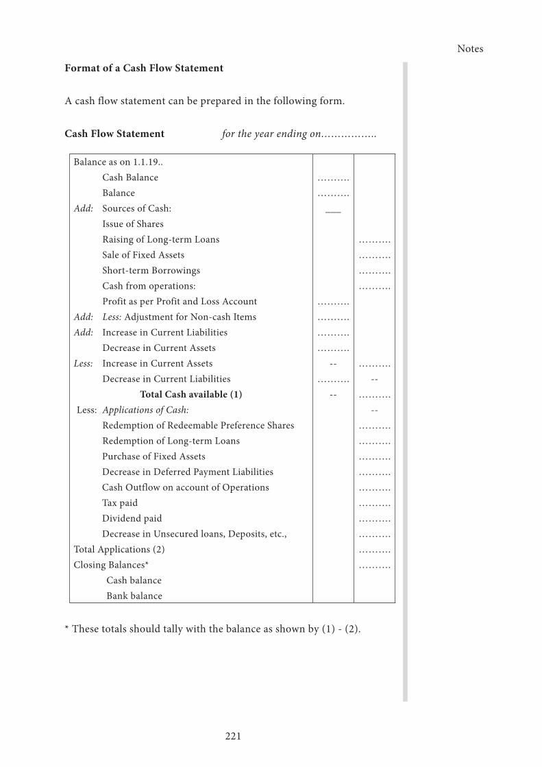
Notes

221

Format of a Cash Flow Statement

A cash flow statement can be prepared in the following form.

Cash Flow Statement for the year ending on……………..

Balance as on 1.1.19.. Cash Balance BalanceAdd: Sources of Cash: Issue of Shares Raising of Long-term Loans Sale of Fixed Assets Short-term Borrowings Cash from operations: Profit as per Profit and Loss AccountAdd: Less: Adjustment for Non-cash ItemsAdd: Increase in Current Liabilities Decrease in Current AssetsLess: Increase in Current Assets Decrease in Current Liabilities

Total Cash available (1) Less: Applications of Cash: Redemption of Redeemable Preference Shares Redemption of Long-term Loans Purchase of Fixed Assets Decrease in Deferred Payment Liabilities Cash Outflow on account of Operations Tax paid Dividend paid Decrease in Unsecured loans, Deposits, etc.,Total Applications (2)Closing Balances* Cash balance Bank balance

……….……….

___

……….……….……….……….

--……….

--

……….……….……….……….

……….--

……….--

………. ……….……….……….……….……….……….……….……….……….

* These totals should tally with the balance as shown by (1) - (2).

Notes

222

Difference Between Cash Flow Analysis and Funds Flow Analysis

Following are the points of difference between a Cash Flow Analysis and a Funds Flow Analysis:

(1) A Cash Flow Statement is concerned only with the change in cash position while a Funds Flow statement is concerned with change in working capital position between two balance sheet dates. Cash is only one of the constituents of working capital besides several other constituents such, as inventories, accounts receivable, prepaid expenses.

(2) A Cash Flow Statement is merely a record of cash receipts, and ‘disbursements. Of course, it is valuable in its own way but it fails to bring to light many important changes involving the disposition of resources. While studying the short-term solvency of a business one is interested not only in cash balance but also in the assets which are easily convertible into cash.

(3) Cash flow analysis is more useful to the management as a tool of financial analysis in short period as compared to funds flow analysis. It has rightly been said that shorter the period covered by the analysis, greater is the importance of cash flow analysis. For example, if it is to be found out whether the business can meet its obligations maturing after 10 years from now? A good estimate can be made about firm’s capacity to meet its long-term obligations? If changes in working capital position on account of operations are observed? However, if the firm’s capacity to meet a liability maturing after one month is to be seen, the realistic approach would be to consider the projected change in the cash position rather than an expected change in the working capital position.

(4) Cash is a part of working capital and, therefore, an improvement in cash position results in improvement in the funds position but the reverse is not true. In other words, “inflow of cash” results in “inflow of funds” but “inflow of funds” may not necessarily result in “inflow of cash”. Thus sound funds position does not necessarily mean a sound cash position but a sound cash position generally means a sound funds position.

Notes

223

(5) Another distinction between a cash flow analysis and a funds flow analysis can be made on the basis of the techniques of their preparation. An increase in a current liability or decrease in a current asset results in decrease in working capital and vice versa. While an increase in a current liability or decrease in current asset (other than cash) will result in increase in cash and vice versa,

Some people, as stated earlier, use term ‘Funds’ in a very narrow sense of cash only. In such an event the two terms ‘Funds’ and ‘Cash’ will have synonymous in meanings.

Utility of Cash Flow Analysis

A Cash Flow Statement is useful for short-term planning. A business enterprise needs sufficient cash to meet its various obligations in the near future such as payment for purchase of fixed assets, payment of debts maturing in the near future, expenses of the business, etc. A historical analysis of the different sources and applications of cash will enable the management to make reliable cash flow projections for the immediate future. It may then plan out for investment of surplus or meeting the deficit, if any. Thus, a cash flow analysis is an important financial tool for the management. Its chief advantages are as follows:

1. Helps in Efficient Cash Management

Cash flow analysis helps in evaluating financial policies and cash position. Cash is the basis for all operations and hence a projected cash flow statement will enable the management to plan and co-ordinate the financial operations properly. The management can know how much cash is needed, from which source it will be derived, how much can be generated internally and how much could be obtained from outside.

2. Helps in Internal Financial Management

Cash flow analysis provides information about cash which will be available from operations. This will help the management in determining policies regarding internal financial management, e.g., possibility of repayment of long-term debt, dividend policies, planning replacement of plant and machinery, etc.

Notes

224

3. Discloses the Movements of Cash

Cash flow statement discloses the complete story of cash movement. The increase in or decrease of, cash and the reason therefore can be known. It discloses the reasons for low cash balance in spite of heavy operating profits or for heavy cash balance in spite of low profits. However, comparison of original forecast with the actual results highlights the trends of movement of cash which may otherwise go undetected.

4. Discloses Success or Failure of Cash Planning

The extent of success or failure of cash planning can be known by comparing the projected cash flow statement with the actual cash flow statement and necessary remedial measures can be taken.

Limitations of Cash Flow Analysis

Cash flow analysis is a useful tool of financial analysis. However, it has its own limitations. These limitations are as under:

(1) Cash flow statement cannot be equated with the Income Statement. An Income Statement takes into account both cash as well as non-cash items and, therefore, net cash flow does not necessarily mean net income of the business.

(2) The cash balance as disclosed by the cash flow statement may not represent the real liquid position of the business since it can be easily influenced by postponing purchases and other payments.

(3) Cash flow statement cannot replace the Income Statement or the Funds Flow Statement. Each of them has a separate function to perform.

In spite of these limitations, it can be said that cash flow statement is a useful supplementary instrument. It discloses the volume as well as the speed at which the cash flows in the different segments of the business. This helps the management in knowing the amount of capital tied up in a particular segment of the business. The technique of cash flow analysis, when used in conjunction with ratio analysis, serves as a barometer in measuring the profitability and financial position of the business.

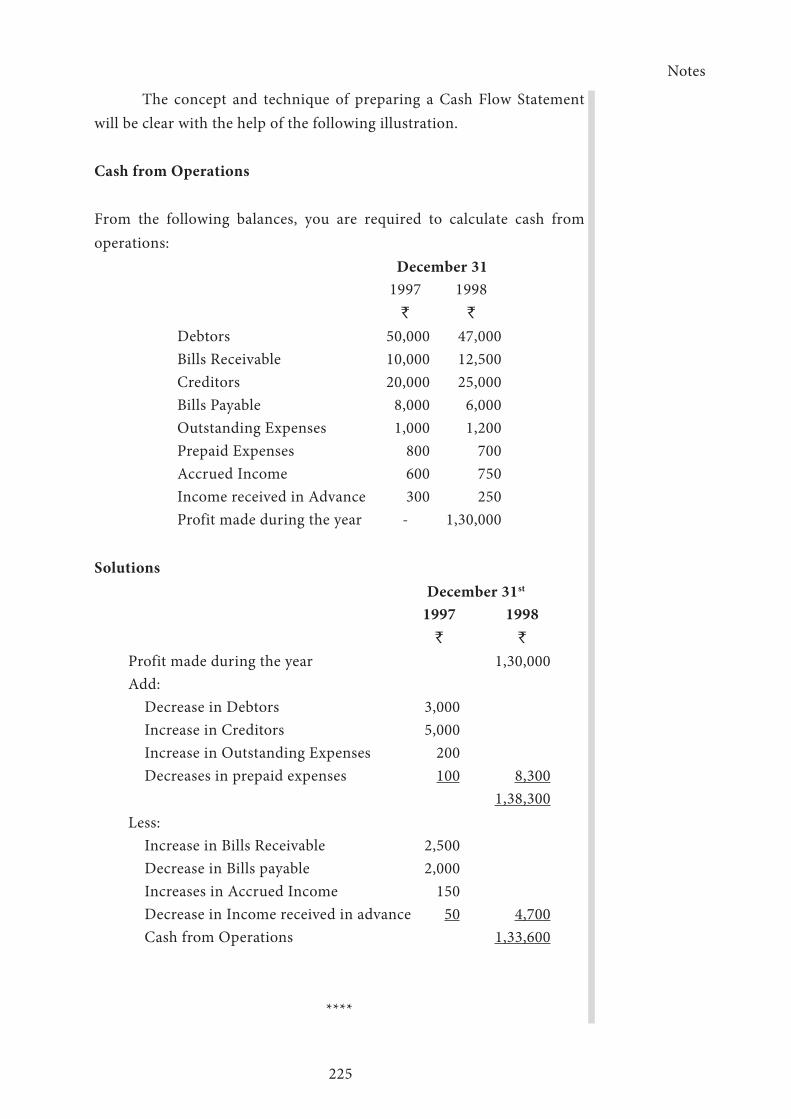
Notes

225

The concept and technique of preparing a Cash Flow Statement will be clear with the help of the following illustration.

Cash from Operations

From the following balances, you are required to calculate cash from operations: December 31

1997`

1998`

Debtors 50,000 47,000Bills Receivable 10,000 12,500Creditors 20,000 25,000Bills Payable 8,000 6,000Outstanding Expenses 1,000 1,200Prepaid Expenses 800 700Accrued Income 600 750Income received in Advance 300 250Profit made during the year - 1,30,000

Solutions December 31st

1997`

1998`

Profit made during the year 1,30,000Add: Decrease in Debtors 3,000 Increase in Creditors 5,000 Increase in Outstanding Expenses 200 Decreases in prepaid expenses 100 8,300

Less:1,38,300

Increase in Bills Receivable 2,500 Decrease in Bills payable 2,000 Increases in Accrued Income 150 Decrease in Income received in advance 50 4,700 Cash from Operations 1,33,600

****

Notes

226

Lesson 4.4 - Contemporary Issues in Management Accounting

Value Chain Analysis; Activity-Based Costing; Quality costing; Target and Life-Cycle Costing and Theory of Constraints Accounting (TOC)

Value Chain Analysis

Value chain is the linked set of value-creating activities from the basic raw material sources for suppliers to the ultimate end-use product delivered into the final customers’ hands. No individual firm is likely to span the entire value chain. Each firm must be understood in the context of the overall value chain of value-creating activities. Note that the value chain requires an external focus, unlike conventional management accounting in which the focus is internal to the firm. According to Michael Porter, a business unit can develop a sustainable competitive advantage based on cost or on differentiation or on both.

The primary focus of the low-cost strategy is to achieve low cost relative to competitors. Cost leadership can be achieved through, for example, economies of scale of production, learning curve effects, tight cost control, cost minimization in R&D, service sales force, or administration. Examples of companies following the low-cost strategy are Nirma in detergents, Shiva in computers, and Times in wrist watches.

The differentiation strategy consists in differentiating the product by creating something perceived as unique. Product differentiation can be achieved through brand loyalty, superior customer service, dealer network, and product design and features. Examples of companies following the differentiation route are Hindustan Lever in detergents, WIPRO in computers and Titan in wrist watches.

Whether or not a firm can develop and sustain differentiation or cost advantage or differentiation with cost advantage depends on how well the firm manages its value chain relative to the value chain of its

Notes

227

competitors. Value chain analysis is essential to determine exactly where in the chain customer value can be enhanced or costs lowered.

It should be noted that no single firm, spans the entire value chain in which it operates. Typically, a firm is only a part of the larger set of activities in the value delivery system. The value chain concept highlights four profit improvement areas:

l. Linkages with suppliers

2. Linkages with customers

3. Process linkages within the value chain of a business unit

4. Linkages across business unit value chain within.

Activity-Based Costing

Applying overhead costs to each product or service based on the extent to which that product or service causes overhead cost to be incurred, is the primary objective of accounting for overhead costs. In many production processes, when overhead is applied to products is used a single pre-determined overhead rate based on a single activity measure. With Activity-Based Costing (ABC), multiple activities are identified in the production processes that are associated with costs. The events within these activities that cause work (costs) are called cost drivers. Examples of overhead cost drivers are machine setups, material-handling operations, and the number of steps in a manufacturing process. Examples of costs drivers in non-manufacturing organizations are hospital beds occupied, the number of take-offs and lending for an airline, and the number of rooms occupied in a hotel. The cost drivers are used to apply overhead to products and services when using ABC.

The following five steps are used to apply costs to products under an ABC system:

1. Choose appropriate activities

2. Trace costs to activities

3. Determine cost drivers for each activity

4. Estimate the application rate for each cost driver

5. Apply costs to products.

Notes

228

These steps are discussed in more detail above.

Choose Appropriate Activities

Involve producing a product or providing a service. The various activities within an organization. The first step of ABC is to choose the activities that will be the intermediate cost objectives of overhead costs. These activities do not necessarily coincide with existing departments but rather represent a group of transactions that support the production process. Typical activities used in ABC are designing, ordering, scheduling, moving materials, controlling inventory, and controlling quality.

Each of these activities is composed ‘of transactions that result in costs. More than one cost pool can be established for each activity. A cost pool is an account to record the costs of an activity with a specific cost driver.

Trace Costs to Activities

Once the activities have been chosen, costs must be traced to the cost pools for different activities. To facilitate this tracing, cost drivers are chosen to act as vehicles for distributing costs. These cost drivers are often called resource drivers. A pre-determined rate is estimated for each resource driver. Consumption of the resource driver in combination with the pre-determined rate determines the distribution of the resource costs to the activities.

Determine Cost Drivers for Activities

Cost drivers for activities are sometimes called activity drivers. Activity drivers represent the event that causes costs within an activity. For example, activity drivers for the purchasing activity include negotiations with vendors, ordering materials, scheduling’ their arrival, and perhaps inspection. Each of these activity drivers represents costly procedures that are performed in the purchasing activity. An activity driver is chosen for each cost pool. If two cost pools use the same cost driver, then the cost pools could be combined for product-costing purposes.

Notes

229

Cooper has developed several criteria for choosing activity drivers. First, the data on the cost driver must be easy to obtain. Second, the consumption of the activity implied by the activity driver should be highly correlated with the actual consumption of the activity. The third criterion to consider is the behavioral effects induced by the choice of the activity driver. Activity drivers determine the application of costs, which in turn can affect individual performance measures.

The judicious use of more activity drivers increases the accuracy of product costs. Ostrenga concludes that there is a preferred sequence for accurate product costs. Direct costs are the most accurate in applying costs to products. The application of overhead costs through cost drivers is the next most accurate process. Any remaining overhead costs must be allocated in a somewhat arbitrary manner, which is less accurate.

Estimate Application Rates for each Activity Driver

An application rate must be estimated for each activity driver. A pre-determined rate is estimated by dividing the cost pool by the estimated level of activity of the activity driver. Alternatively, an actual rate is determined by dividing the actual costs of the cost pool by the actual level of activity of the activity driver. Standard costs, could also be used to calculate a pre-determined rate.

Applying Costs to Products

The application of costs to products is calculated by multiplying the application rate times the usage of the activity driver in manufacturing a product or providing a service.

Examples of Activity-Based Costing

Modison Motors Inc. produces electric motors. The company makes a standard electric-starter motor for a major auto manufacturer and also produces electric motors that are specially ordered. The company has four essential activities: design, ordering, machinery, and marketing. Modison Motors incurs the following costs during the month of, January:

Notes

230

Standard Motors Special Order MotorsDirect Labor ` 10,00,000 ` 2,00,000Direct materials ` 30,00,000 ` 10,00,000Overhead:Indirect labour ` 3,50,000Depreciation of building ` 2,00,000Depreciation of equipment

` 10,00,000

Maintenance ` 3,00,000Utilities ` 10,00,000

` 60,00,000

Traditional cost accounting would apply the overhead costs based on a single measure of activity. If direct labor dollars were used, then the overhead rate would be ` 60, 00,000 / (` 10, 00,000 + ` 2, 00,000), or ` 5, per direct-labor dollar. Hence: Overhead to standard motors

= (` 5/Direct-labor dollar)(` 10,00,000 of direct labor) = ` 50,00,000

Overhead to special-order motors

= (` 5/Direct-labor dollar)(` 2,00,000 of direct labor) = ` 10,00,000

With ABC, activities are chosen and the overhead costs are distributed to cost pools within these activities through resource drivers. The costs of activities are then applied to products through activity drivers. Suppose that Modison Motors uses the following activities: designing, ordering, machining, and marketing. Each activity has one cost pool. The overhead costs are distributed to the cost pools of the activities using the following resource drivers:

Overhead Account Resource Driver

Indirect labor Labor dollars

Depreciation of building Square feet of building

Depreciation of equipment Machine time

Maintenance Square feet of building

Utilities Amps used

Notes

231

The usages of the resource drivers by activity are:

Designing Ordering Machining Marketing TotalsLabor Dollars 10,00,000 20,000 1,00,000 1,30,000 3,50,000Sq.ft of building 50,000 30,000 1,00,000 20,000 2,00,000Machine time 0 0 10,00,000 0 10,00,000Amps 2,00,000 1,00,000 16,00,000 1,00,000 20,00,000

The resource driver application rates are calculated by dividing overhead costs by total resource driver usage:

Overhead Account

Resource DriverCost of

Overhead Total Driver

UsageApplication

Rate

Indirect labor Labor dollars ` 35,00,000 ` 3,50,000`,10/ Labor dollar

Depreciation of building

Square feet of building

2,00,000 2,00,000 Sqft ` 1/sq.ft.

Depreciation of machinery

Machine time 10,00,000 50.000 hrs. ` 20/hr.

Maintenance Sq. ft. of building 3,00,000 2,00,000 sqft. ` 1.50/sq.ft.Utilities Amps used 10.00.000 20,00,000 amps 0.50/amp

By multiplying the application rate times the resource usage of each activity, overhead costs can be allocated to the different activities. For example, the cost of the indirect labor allocated to the designing activity is ` 10/labor dollar times ` 10,000 in labor, or ` 100,000.

Designing Ordering Machining Marketing Total` ` ` ` `

Indirect labor 10,00,000 2,00,000 10,00,000 13,00,000 35,00,000Depreciat ion of building

50,000 30,000 1,00.000 20,000 2,00,000

Depreciat ion of equipment

10,00,000 10,00,000

Maintenance 75,000 45,000 1,50,000 30.000 3,00,000Utilities 1,00,000 50,000 8,00,000 50,000 10,00,000Total 12,25.000 3,25,000 30,50,000 14,00,000 60,00,000

Once the overhead costs have been distributed to the activity cost pools, activity drivers must be chosen to apply the costs to the.products. Suppose the following activity drivers are chosen:

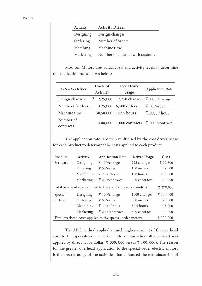
Notes

232

Activity Activity Driver

Designing Design changes

Ordering Number of orders

Matching Machine time

Marketing Number of contract with customer

Modison Motors uses actual costs and activity levels to determine the application rates shown below:

Activity DriverCosts of Activity

Total Driver Usage

Application Rate

Design changes ` 12,25,000 12,250 changes ` 1 00 /change

Number 0f orders 3.25,000 6,500 orders ` 50 /order

Machine time 30,50.000 152.5 hours ` 2000 / hour

Number of contracts

14.00,000 7,000 contracts ` 200 /contract

The application rates are then multiplied by the cost driver usage for each product to determine the costs applied to each product.

Product Activity Application Rate Driver Usage CostStandard Designing ` 100/change 225 changes ` 22,500

Ordering ` 50/order 150 orders 7,500 Machining ` 2000/hour 100 hours 200,000 Marketing ` 200/contract 200 contracts 40,000

Total overhead costs applied to the standard electric motors ` 270,000

Special- Designing ` 100/change 1000 changes ` 100,000ordered Ordering ` 50/order 500 orders 25,000

Machining ` 2000 / hour 52.5 hours 105,000Marketing ` 200 /contract 500 contract 100,000

Total overhead costs applied to the special-order motors ` 330,000

The ABC method applied a much higher amount of the overhead cost to the special-order electric motors than when all overhead was applied by direct-labor dollar (` 330, 000 versus ` 100, 000). The reason for the greater overhead application to the special-order electric motors is the greater usage of the activities that enhanced the manufacturing of

Notes

233

the electric motors during their production. Use of direct-labor dollars to allocate overhead does not recognize the extra overhead requirements of the special-order electric motors. Misapplication of overhead could lead to inappropriate product line decisions.

The greater the diversity of requirements of products on overhead-related services and other overhead costs, the greater the need for an ABC system.

Other Benefits of Activity-Based Costing

ABC is valuable for planning, because the establishment of an ABC system requires a careful study of the total manufacturing or service process of an organization. ABC highlights the causes of costs. An analysis of these causes can identify activities that do not add to the value of the product. These activities include moving materials and accounting for transactions. Although these activities cannot be completely eliminated, they may be reduced. Recognition of how various activities affect costs can lead to modifications in the planning of factory layouts and increased efforts in the design process stage to reduce future manufacturing costs.

An analysis of activities can also lead to better performance measurement. Workers on the line often understand activities better than costs and can be evaluated accordingly. At higher management levels, the activities can be aggregated to coincide with responsibility centers. Managers would be responsible for the costs of the activities associated with their responsibility centers.

Weaknesses of Activity-Based Costing

First, ABC is based on historical costs. For planning decisions, future costs are generally the relevant costs. Second, ABC does not divide variable and fixed costs. For many short run decisions, it is important to identify variable costs. Third, ABC is only as accurate as the quality of the cost drivers. The distribution and application of costs becomes an arbitrary allocation process when the cost drivers are not associated with the factors that are causing costs. And finally, ABC tends to be more costly than the more traditional methods of applying costs to products.

Notes

234

Quality Costing

The benefits from increased product quality come in lower costs for reworking discovered defective units and from more satisfied customers who find fewer defective units. The cost of lowering the tolerance for defective units results from the increased costs of using a better production technology. These costs could be due to using more highly skilled and experienced workers, from using a better grade of materials, or from acquiring updated production equipment.

A quality-costing system monitors and accumulates the costs incurred by a firm in maintaining or improving product quality.

Measuring Quality Costs

The quality costs discussed here deal with costs associated with quality of conformance as opposed to costs associated with quality of design. Quality of design refers to variations in products that have the same functional use.

Quality of Conformance refers to the degree with which the final product meets its specifications. In other words, quality of conformance refers to the product’s fitness for use. If products are sold and they do not meet the consumers’ expectations, the company will incur costs because the consumer is unhappy with the product’s performance. These costs are one kind of quality costs that will be reduced if higher-quality products are produced. Thus higher quality may mean lower total costs when quality of conformance is considered.

The costs associated with quality of conformance generally can be classified into four types: prevention costs, appraisal costs, internal failure costs, and external failure costs. The prevention and appraisal costs occur because a lack of quality of conformance can exist. The internal and exter-nal failure costs occur because a lack of quality of conformance does exist.

Prevention Costs are the costs incurred to reduce the number of defective units produced or the incidence of poor-quality service. Prevention costs begin with the designing and engineering of the product or service. Designers and engineers should work together to develop a product that is easy to assemble with a minimal number of mistakes.

Notes

235

Appraisal Costs are the costs incurred to ensure that materials, products, and services meet quality standards. Appraisal costs begin with the inspection of raw materials and part from vendors. Further inspection costs are incurred throughout the production process. Quality audits and reliability tests are performed on products and services to determine if they meet quality standards. Appraisal costs also occur through field inspections at the customer site before the final release of the product.

Internal Failure Costs are the costs associated with materials and products that fail to meet quality standards and result in manufacturing losses. These defects are identified before they are shipped to customers. Scrap and the costs of spoiled units that cannot be salvaged are internal failure costs. The cost of analyzing, investigating and reworking defects is also internal failure costs. Defects create additional costs because they lead to down time in the production process.

External Failure Costs are the costs incurred when inferior-quality products or services are sold to customers. These costs begin with customer complaints and usually lead to warranty repairs, replacement, or product recall.

The problem management faces is choosing the desired level of product quality. If all the costs can be measured accurately, then the desired level of product quality occurs when the sum of prevention, appraisal, and failure costs is minimized. Quality costs are minimized at a specific percentage of planned defects.

The magnitude of quality costs has prompted many companies to install quality-costing systems to monitor and help reduce the costs of achieving high-quality production. Several examples follow.

➢ Quality at Bavarian Motor Works (BMW)

➢ Quality Costs in Banking

➢ Reducing Quality Costs at TRW

➢ Cost of a faulty electrical component at Hewlett-Packard

Although the concepts of quality costing are easy to understand, the cost measurement of many quality efforts is difficult. Many of the costs are not isolated in a traditional cost accounting system, and some costs are opportunity costs that are not part of a historical cost accounting system.

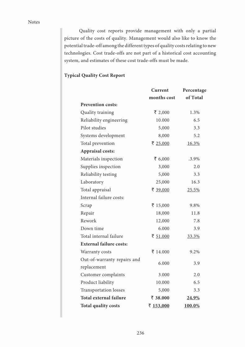
Notes

236

Quality cost reports provide management with only a partial picture of the costs of quality. Management would also like to know the potential trade-off among the different types of quality costs relating to new technologies. Cost trade-offs are not part of a historical cost accounting system, and estimates of these cost trade-offs must be made.

Typical Quality Cost Report

Current Percentage months cost of Total

Prevention costs:Quality training ` 2,000 1.3%Reliability engineering 10.000 6.5Pilot studies 5,000 3.3Systems development 8,000 5.2Total prevention ` 25,000 16.3%Appraisal costs:Materials inspection ` 6,000 .3.9%Supplies inspection 3,000 2.0Reliability testing 5,000 3.3Laboratory 25,000 16.3Total appraisal ` 39,000 25.5%Internal failure costs:Scrap ` 15,000 9.8%Repair 18,000 11.8Rework 12,000 7.8Down time 6.000 3.9Total internal failure ` 51.000 33.3%External failure costs:Warranty costs ` 14.000 9.2%Out-of-warranty repairs and replacement

6.000 3.9

Customer complaints 3.000 2.0Product liability 10.000 6.5Transportation losses 5,000 3.3Total external failure ` 38.000 24.9%Total quality costs ` 153,000 100.0%

Notes

237

Total Quality Control

Total quality control (TQC) is a management process based on the belief that quality costs are minimized with zero defects. The phrase quality is free is commonly advocated by proponents of TQC, who argue that the reduction of failure costs due to improved quality outweigh additional prevention and appraisal costs.

It is not surprising, then, that U.S. Auto Manufacturers have recently become leaders in advocating TQC.

TQC begins with the design and engineering of the product. Designing a product to be resistant to workmanship defects may not be incrementally more costly than the present design process, but the reduction in other quality costs can be substantial.

TQC is often associated with just-in-time (JIT) manufacturing. Under JIT each worker is trained to be a quality inspector. Therefore teams specializing in quality inspection become unnecessary. With suppliers delivering high-quality parts and materials, a company can substantially reduce, if not eliminate appraisal costs.

Total quality control is sometimes referred to as total quality management (TQM) because a completely new orientation must be taken by management to make TQC successful. New performance measures that reinforce quality improvements must be initiated. Standard cost variance such as the materials price variance and labor efficiency variance tend to emphasize price and quantity rather than quality and should not be used to reward employees. The productivity measures described in the next section are more useful in motivating workers to achieve both quality and productivity.

Target Costing

Introduction

Target costing has recently received considerable attention. Computer Aided Manufacturing-International defines target cost as “a market-based cost that is calculated using a sales price necessary to capture a predetermined market share.” In competitive industries a unit

Notes

238

sales price would be established independent of the initial product cost. If the target cost is below the initial forecast of product cost, the company drives the unit cost down over a designed period to compete.

Target cost = Sales price (for the target market share) - Desired profit

Japanese cost management is known to be guided by the concept of target cost. Management decides, before the product is designed, what a product should cost, based on marketing (rather than manufacturing) factors. The following write-up on target costing for the Sony Walkman describes the target costing approach.

The Walkman: Setting the price before the Cost

Sony’s Walkman was a classic example of how a company uses the “PROFITS = SALES - COSTS” equation to full advantage: First set the price at which the customer will buy, then bring down your costs so you can make profits. “I dictated the selling price (of the Walkman) to suit a young person’s pocketbook, even before we made the first machine,” wrote Sony Corp. Chairman Akio Morita in his book Made In Japan. “I said I wanted the first models... to retail for no more than Yen 30,000. The accountants protested but I persisted. I told them I was confident we would be making our new product in very large numbers and our cost would come down as volume climbed.”

The target costing philosophy leads to a market-driven approach to accounting. Target costs are conceptually different from standard costs. Standard costs are predetermined costs built up from an internal analysis by industrial engineers. Target costs are based on external analysis of markets and competitors. Several Japanese firms are known to compute two separate variances, one comparing actual costs with target costs and other comparing actual costs with standard costs.

While introducing a new product, a company might test the market to determine the price it can charge in order to be competitive with products already on the market of similar function and quality. A target cost is the maximum manufactured cost for a product. It is arrived at by subtracting its expected market price from the required margin on sales.

Notes

239

Target costing is a market-driven design methodology. It estimates the cost for a product and then designs the product to meet that cost. It is used to encourage the various departments involved in design and production to find less expensive ways of achieving similar or better product features and quality.

It is a cost management tool which reduces a product’s costs over its entire life cycle. Target costing includes actions the management needs to take i.e. establish reasonable target costs, develop methods for achieving those targets, and develop means by which to test the cost effectiveness of different cost-cutting scenarios.

There are several phases to the methodology.

Conception (Planning) Phase

Based upon its strategic business plans, a company must first establish what type of product it wishes to manufacture.

Traditionally (before target costing), once the type of product was determined, its development was assigned to the product design department. Then the produced product was sent to the costing department, which assessed the cost of the design and frequently found it more expensive to produce than the market would tolerate.

The design was then returned to the design department with instructions to reduce its costs, usually by promising its quality. The product design was sent back and forth between the two departments until consensus was reached. The product was then sent to the manufacturing department, which often concluded that it was impossible to manufacture it in its proposed cost. It was then sent back to the design department, so on. Much time, money and effort were spent before the product reached the production stage. As a result, profit suffered.

Under target costing, a product’s design begins at the opposite end. It first establishes a price at which the product can be competitive and then assigns a team to develop cost scenarios and search for ways to design the product to meet those cost constraints. Several steps must be taken in order to establish a reasonable target cost.

Notes

240

i) Market research should be done to determine several factors. First, the products of competitors’ should be analyzed with regard to price, quality, service and support, delivery, and technology. After a preliminary test of competitor’s product, it is necessary to establish the features that consumers’ value in this type of product, and the important features that are lacking.

ii) After preliminary testing, a company should be able to pinpoint a market niche it believes is undersupplied, and in which it believes it might have some competitive advantage. Only then can a company set a target cost close to competitors’ products of similar functions and value. The target cost is bound to change in the development and design stages. However, the new target costs should only be allowed to decrease, unless the company can provide added features that add value to the product.

Development Phase

The company must find ways to attain the target cost. is involves a number of steps.

1. First, an in-depth study of the most competitive product on the market must be conducted. This study will show what materials were used and what features are provided, and it will give an indication of the manufacturing process needed to complete the product.

Once a better understanding of the design has been achieved, the organization can target the costs against this “best” design. But its competition will probably be engaged in similar analysis and will further improve its product toward this “best” design. It is necessary when performing comparative cost analysis, and trying to establish the competitor’s cost structure, adequate attention be paid to the competitive advantages of the competitor, such as technology, location, and vertical integration.

2. After trying to identify the cost structure of the competitor, the company should develop estimates for the internal cost structure of its own products. This is most effectively done by analyzing

Notes

241

internal costs’ of similar products already being produced by the company and should take into account the different needs of the new product in assessing these costs.

3. After preliminary analysis of the cost structures of both the competition and itself, the company should further define these cost structures in terms of cost drivers. Focusing on cost drivers can help reduce waste, improve quality, minimize non-value-added activities, and identify ineffective product design. The use of multiple drivers’ leads both to a better understanding of the inputs and resources required to produce products, and a better cost analysis through more detailed cost information.

When enough cost information is available, the product development team is able to generate cost estimates under different scenarios. After this, the designers, manufacturers, marketers, and engineers on the team should conduct a session of brainstorming to generate ideas on how to substantially reduce costs (by smoothing the process, using different materials, and so on) or add a number of different features to the product without increasing target costs. In these brainstorming sessions, no idea is rejected, and the best ideas are integrated into the development of the product.

Production Phase

In these stages, target costing becomes a tool for reducing costs of existing products. It is highly unlikely that the design, manufacturing, and engineering groups will develop the optimal, cost-effective process at the beginning of production. The search for better, less expensive products should continue in the framework of continuous improvement.

1. The ABC technique can be useful as a tool for target costing of existing products. ABC assists in identifying non value-added activities and can be used to develop scenarios on how to minimize them. Target costing at the activity level makes opportunities for cost reduction highly visible.

2. Target costing is also strongly linked to consumer requirement, and tries to identify the features such as performance specifications, services, warranties, and delivery consumers want products to

Notes

242

provide. These consumers may also be questioned about which features they prefer in products, and how much they are worth to them. The surveys on preferable features and value of these features help management do cost-benefit analysis on different features of a product, and then try to reduce costs on features that are not ranked highly.

3. Target costing also provides incentives to move toward less expensive means of production, as well as production techniques that provide a more even flow of goods. JIT provides an environment where there is better monitoring of costs and product quality as well as access to ideas for continuous improvement and better production strategies.

Benefits of Target Costing

1. The process of target costing provides detailed information on the costs involved in producing a new product, as well as a better way of testing different cost scenarios through the use of ABC.

2. Target costing reduces the development cycle of a product. Costs can be targeted at the same time the product is being designed, bringing in the resources of the manufacturing and finance departments to ensure that all avenues of cost reduction are being explored and that the product is designed for manufacturability at an early stage of development.

3. The internal costing model, using ABC, can provide an excellent understanding of the dynamics of production costs and can detail ways to eliminate waste, reduce non-value-added activities, improve quality, simplify the process, and attack the root causes of costs (cost drivers). It can also be used for measuring different cost scenarios to ensure that the best ideas available are incorporated from the outset into the production design.

4. The profitability of new products is increased by target costing through promoting reduction in costs while maintaining or improving quality. It also helps in promoting the requirements of consumers, which leads to products that better reflect consumer needs and find better acceptance than existing products.

Notes

243

5. Target costing is also used to forecast future costs and to provide motivation to meet future cost goals.

6. Target costing is very attractive because it is used to control costs before the company even incurs any production costs, which saves a great deal of time and money.

7. Drawback of target costing: - There is one major drawback to target costing. It is difficult to use with complex products that require many subassemblies, such as automobiles. This is because tracking costs becomes too complicated and tedious, and cost analysis must be performed at so many levels.

Life Cycle Costing

CAM-l defines life-cycle costing as “the accumulation of costs for activities that occur over the entire life cycle of a product, from inception to abandonment by the manufacturer and the customer,” Life-cycle analysis provides a framework for managing the cost and performance of a product over the duration of its life.

The life-cycle commences with the initial identification of a consumer need and extends through planning, research, design, development, production, and evaluation, and use, logistics support in operation, retirement, and disposal. Life-cycle is important to cost control because of the interdependencies of activities in different time periods. For example, the output of the design activity has a significant impact on the cost and performance of subsequent activities.

Cost systems have focused primarily on the cost of physical production, without accumulating costs over the entire design, manufacture, market, and support cycle of a product. Resources committed to the development of products and the manufacturing process represents a sizeable investment of capital. The benefits accrue over many years, and under conventional accounting, are not directly identified with the product being developed. They are treated instead as a period expense and allocated to all products. Even companies which use life-cycle models for planning and budgeting new products do not integrate these models into cost systems. It is important to provide feedback on planning effectiveness and the impact of design decisions on operational and support costs.

Notes

244

Period reporting hinders management’s understanding of product-line profitability and the potential cost impact of long-term decisions such as engineering design changes. Life-cycle costing and reporting provide management with a better picture of product profitability and help managers to gauge their planning activities.

Product Life Cycle Costing

The cycle begins with the identification of new consumer need and the invention of a new product and is often followed by patent protection and further development to make it saleable.

This is usually followed by a rapid expansion in its sales as the product gains market acceptance. Then competitors enter the field with imitation and rival products and the distinctiveness of the new product starts diminishing. The speed of degeneration differs from product to product. The innovation of a new product and its degeneration into a common product is termed as the ‘life cycle of a product’.

Characteristics

The major characteristics of product life-cycle concept are as follows:

➢ The products have finite lives and pass through the cycle of development, introduction, growth, maturity, decline and deletion at varying speeds.

➢ Product cost, revenue and profit patterns tend to follow predictable courses through the product life cycle. Profits first appear during the growth phase and after stabilizing during the maturity phase, decline thereafter to the point of deletion.

➢ Profit per unit varies as products move through their life cycles.

➢ Each phase of the product life-cycle poses different threats and opportunities that give rise to different strategic actions.

➢ Products require different functional emphasis in each phase - such as an R&D emphasis in the development phase and a cost control emphasis in the decline stage.

Notes

245

Activities in Product Life Cycle

Typically the life cycle of a manufactured product will consist of the following activities:

1. Market research

2. Specification

3. Design

4. Prototype manufacture

5. Development of the product Tooling

6. Manufacturing

7. Selling

8. Distribution

9. Product support through after sales service

10. Decommissioning or Replacement.

Phases in Product Life-Cycle

There are five distinct phases in the life cycle of a product as shown.

Introduction phase: The Research and engineering skills lead to product development and when the product is put on the market and its awareness and acceptance are minimal. Promotional costs will be high, sales, revenue low and profits probably negative. The skill that is exhibited in testing and launching the product’ will rank high in this phase as critical factor in securing success and initial market acceptance. Sales of new products usually rise slowly at first.

Despite little competition profits are negative or low. This owns to high unit costs resulting from low output rates, and heavy promotional investments incurred to stimulate growth. The introductory stage may last from a few months to a year for consumer goods and generally longer for industrial products.

Growth phase: In the growth phase product penetrates into the market and sales increases because of the cumulative effects of introductory promotion, distribution. Since costs will be lower than in the earlier phase, the product will start to make a profit contribution. Following the

Notes

246

consumer acceptance in the launch phase it now becomes vital to secure wholesaler/retailer support. But to sustain growth, consumer satisfaction must be ensured at this stage. If the product is successful, growth usually accelerates at some point, often catching the innovator by surprise.

Profit margins peak during this stage as ‘experience curve’ affects lower unit costs and promotion costs are spread over a larger volume.

Maturity phase: This stage begins after sales cease to rise exponentially. The causes of the declining percentage growth rate the market saturation eventually may be because most potential customers have tried the product and sales settle at a rate governed by population growth and the replacement rate of satisfied buyers. In addition there are no new distribution channels to fill. This is usually the longest stage in the cycle, and most existing products are in this stage. The period over which sales are maintained depends upon the firm’s ability to stretch, the cycle by means of market segmentation and finding new uses for it.

Profits decline in this stage because for the following reasons.

➢ The increasing number of competitive products.

➢ The innovators find market leadership under growing pressure.

➢ Potential cost economies are used up.

➢ Prices begin to soften as smaller competitors struggle to obtain market share in an increasingly saturated market.

Sales growth continues but at a diminishing rate because of the diminishing number of potential customers. It may happen certain unsuccessful competing brands would have withdrawing from the market. For this reason sales are likely to continue to rise while the customers for the withdrawn brands are mopped up by the survivors. In this phase there will be stable prices and profits and the emergence of competitors. There is no improvement in the product but changes in selling effort are common, profit margin slip despite rising sales.

Saturation phase: As the market becomes saturated, pressure is exerted for a new product as profit begins to fall. Intensified marketing effort may prolong the period of maturity, but only by increasing costs disproportionately.

Notes

247

Decline phase: Eventually most products and brands enter a period of declining sales. This may be caused by the following factors:

➢ Technical advances leading to product substitution.

➢ Fashion and changing tastes.

➢ The average length of the product life cycle is tending to shorten as a result of economic, technological and social change.

Turning Point Indices in Product Life Cycle

The following checklist indicates some of the detailed information necessary to identify turning points in the product life cycle:

Market Saturation

➢ Is the growth rate of sales volume declining?

➢ What is the current level of ownership compared to potential?

➢ Are first time buyers a declining proportion of total sales?

Nature of Competition

➢ How many competitors have entered or plan to enter?

➢ Is long-term over capacity emerging?

➢ Are prices and profit margins being cut?

➢ Are advertising and promotional elasticity declining and price elasticity increasing?

Alternative Products and Technologies

➢ Are new products being created in this industry by others which may meet consumer needs more effectively?

➢ Is significant technical progress taking place which threatens existing products?

Project Life Cycle Costing

The term ‘project life cycle cost’ has been defined as follows: ‘It includes the costs associated with acquiring, using, caring for and disposing

Notes

248

of physical assets, including the feasibility studies, research, design, development, production, maintenance, replacement and disposal, as well as support, training an operating costs generated by the acquisition, use, maintenance and replacement of permanent physical assets’.

Project Life Cycle Costs

Product life cycle costs are incurred for products and services from their design stage through development to market launch, production and sales, and their eventual withdrawal from the market. In contrast project life cycle costs are incurred for fixed assets, i.e. for capital equipment and so on. The component elements of a project’s cost over its life cycle could include the following:

➢ Acquisition cost, i.e. costs of research, design, testing, production, construction, or purchase of capital equipment.

➢ Transportation and handling costs of capital equipment

➢ Maintenance costs of capital equipment

➢ Operations costs, i.e. the costs incurred in operations, such as energy costs, and various facility and other utility costs.

➢ Training costs i.e. operator and maintenance training.

➢ Inventory costs i.e. cost of holding spare parts, warehousing etc.

➢ Technical data costs, i.e. costs of purchasing any technical data.

➢ Retirement and disposal costs at the end of life or the capital equipment life.

Management Accountants’ Role in Project Life Cycle Costing

Project life-cycle costing is a new concept which places new demands upon the Management Accountant. The development of realistic project life cycle costing models will require the accountant to develop an effective working relationship with the operational researcher and the systems analyst, as well as with those involved in the terro technological system, particularly engineers. Engineers require a greater contribution from accountants in terms of effort and interest throughout the life of a physical asset. A key question for many accountants will be whether the costs of developing realistic life cycle costs will outweigh the benefits to

Notes

249

be derived from their availability. Lifecycle costing in the management of Physical Assets, much value can be obtained by thinking in life-cycle costing concepts whenever a decision affecting the design and operation of a physical asset is to be made.

The concept project life cycle costing has become more widely accepted in recent years. The philosophy of it is quite simple. It involves accounting for all costs over the life of the decision which is influenced directly by the decision.

Terro technology is concerned with pursuit of economic life cycle costs. This simply means trying to ensure that the assets produce the highest possible benefit at least cost. To do this, it is necessary to record the cost of designing, buying, installing, operating, and maintaining the asset, together with a record of the benefits produced. Most organizations keep a record of the initial capital costs, only for asset accounting purposes.

Uses of Project Life Cycle Costing

The project life cycle costing is especially useful in the following areas:-

➢ Projects operate in capital intensive industries

➢ Projects have a sizable, on-going constructing program

➢ Projects dependent on expensive or numerous items of plant with consequent substantial replacement programs

➢ Projects considering major expansion

➢ Projects contemplating the purchase/design/ development of expensive new technology

➢ Projects sensitive to disruption due to down-time.

Theory of Constraints (TOC)

The theory of constraints (TOC) is an overall management philosophy introduced by Eliyahu M. Goldratt in his 1984. The theory of constraints is a process of continuous improvement to clear the throughput chain of all constraints. The profits are expanded by increasing the throughput of the plant. What prevents the throughput being higher is constraint. The theory of constraints describes methods to maximize

Notes

250

operating income when faced with some bottleneck and some non-bottleneck operations. It is now necessary to deal in detail with the terms ‘throughput’ and ‘constraints’.

Five steps in TOC. The Toc as management tool can be explained by considering five steps;

1. Identify the system’s constraint.

2. Decide how to exploit the system’s constraint.

3. Subordinate everything to constraint.

4. Elevate the system’s constraint.

5. Repeat the process, if the constraint is broken.

Application of TOC

➢ Operations

➢ Supply chain / logistics

➢ Finance and accounting

➢ Project management

➢ Marketing and sales

Self Assessment Questions (SAQs)

1. What do you understand by the term funds?

2. What is working capital?

3. Define funds flow statement

4. Distinguish funds flow statement from income statement

5. Distinguish funds flow statement from balance sheet

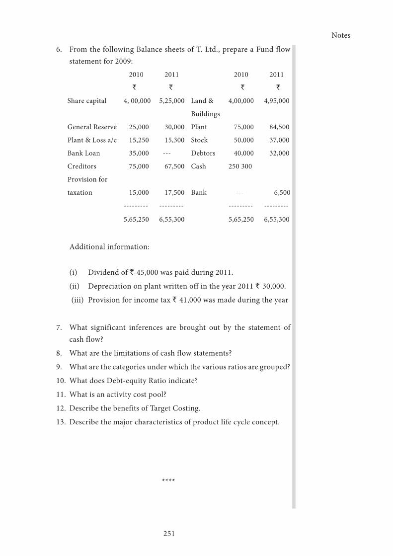
Notes

251

6. From the following Balance sheets of T. Ltd., prepare a Fund flow statement for 2009:

2010 2011 2010 2011

` ` ` `

Share capital 4, 00,000 5,25,000 Land & 4,00,000 4,95,000

Buildings

General Reserve 25,000 30,000 Plant 75,000 84,500

Plant & Loss a/c 15,250 15,300 Stock 50,000 37,000

Bank Loan 35,000 --- Debtors 40,000 32,000

Creditors 75,000 67,500 Cash 250 300

Provision for

taxation 15,000 17,500 Bank --- 6,500

--------- --------- --------- ---------

5,65,250 6,55,300 5,65,250 6,55,300

Additional information:

(i) Dividend of ` 45,000 was paid during 2011.

(ii) Depreciation on plant written off in the year 2011 ` 30,000.

(iii) Provision for income tax ` 41,000 was made during the year

7. What significant inferences are brought out by the statement of cash flow?

8. What are the limitations of cash flow statements?

9. What are the categories under which the various ratios are grouped?

10. What does Debt-equity Ratio indicate?

11. What is an activity cost pool?

12. Describe the benefits of Target Costing.

13. Describe the major characteristics of product life cycle concept.

****

252

Notes

253

UNIT - V

Reporting to Management

Learning Objectives

After studying this unit you will be able to

➢ Understand the concept of social cost benefit analysis

➢ Know the objectives and techniques of social cost benefit analysis

➢ Analyze the difficulties of social cost benefit analysis

➢ The general format of report and Reporting

➢ Importance of Reporting in the Finance field.

Unit Structure

Lesson 5.1 - Social Cost Benefit Analysis

Lesson 5.2 - Reporting to Management

Notes

254

Lesson 5.1 - Social Cost Benefit Analysis

Concept of Social Cost Benefit Analysis

The first objective of financial management i.e. profit maximization has become out of context due to its technical flaws. Social cost-benefit analysis (SCBA) can be defined as “a systematic and quantitative appraisal to determine whether estimated social benefits of a project justify the estimated social costs”. The objectives of a business enterprise are not only making profit but also to take into account of the interests of the stakeholders such as employees, customers, suppliers, government, general public etc. The business should help in overcoming social problems. It should try to help society even at the cost of reducing its profits. This is carried out by corporate through their participation in social responsibility. Generally, cost benefit analysis is necessary in order to allocate the scarce resources among different sectors within the economy and among different projects within each sector of the economy. To determine the rationality of investment in any project undertaken for social betterment as whole, cost benefit analysis is necessary.

Objectives of Social Cost Benefit Analysis

(i) To evaluate the potential future economic and social benefits that may be fetched by the projects that are to be started.

(ii) To estimate the potential future economic and social costs that may be incurred to get the benefits.

(iii) To calculate the net benefits as a result of the above appraisal.

(iv) To ascertain the net benefits that may be received from each of the alternative projects being considered.

(v) To identify projects those will yield the maximum benefits in relation to set economic standard and social goals for the national economy.

Notes

255

Techniques of Social Cost Benefit Analysis

The following are the techniques used in social cost benefit analysis

A. INIDO Methodology

United Nations Industrial Development Organization (UNIDO) has five stages

➢ Calculation of financial profitability measured at market prices

➢ Obtaining the net benefit of the project measured in terms of economic (efficiency) prices

➢ Adjustment for the impact of the project on savings and investment

➢ Adjustment for the impact of the project on income distribution

➢ Adjustment for the impact of the project on merit goods and demerit goods

B. Little and Mirrlee’s Approach (LM Approach)

➢ LM approach uses uncommitted social income basis.

➢ LM approach focuses on an integrated analysis of the consideration such as efficiency, saving and redistribution.

➢ Outputs and inputs of a project are classified by the LM approach into three categories, namely, traded goods /services, non traded goods/services and labor.

Difficulties in Social Cost Benefit Analysis

1. Difficulty of measuring benefits

➢ It is very difficult to measure the benefits of social programme

➢ It is hard to recognize the ancillary benefits of social programme

2. Difficulty of scale problems

Determining the scale of operation is another important problem faced when social cost analysis is done

Notes

256

3. Difficulty in estimating social costs

In estimating social cost of future programmes, two elements of uncertainties need close consideration. These are referred to as cost estimating uncertainty and programme uncertainty. Cost estimating uncertainty happens due to the inability to estimate the cost of certain items. While programme uncertainty refers to the lack of information relating to programme need.

4. Difficulty in determining total cost system

This problem is aroused where inter-relationship of various programme components is missing. In order to estimate social cost, it is important to consider a programme as a total system, but not as a single component.

Decision Tree

A decision tree is a decision support tool that uses a tree-like graph or model of decisions and their possible consequences, including chance event outcomes, resource costs, and utility. It is one way to display an algorithm.

Decision tree is a useful analytical tool for clarifying the range of alternative courses of action and their possible outcomes.

It is a diagram showing several possible courses of action and possible events (i.e.., state of nature) and the potential outcomes for each course of action. It is a graphic representation of the sequence of action- event combinations available to the decision-maker.

A decision tree consists of 3 types of nodes:

1. Decision nodes - commonly represented by squares

2. Chance nodes - represented by circles

3. End nodes - represented by triangles

Decision trees are commonly used in operations research, specifically in decision analysis, to help identify a strategy most likely to reach a goal. If in practice decisions have to be taken online with no

Notes

257

recall under incomplete knowledge, a decision tree should be paralleled by a probability model as a best choice model or online selection model algorithm.

Another use of decision trees is as a descriptive means for calculating conditional probabilities. Decision trees, influence diagrams, utility functions, and other decisions.

****

Notes

258

Lesson 5.2 - Reporting to Management

Introduction

The term ‘reporting’ conveys different meanings on different circumstances. In a narrow sense it means: supplying facts and figures. On the other hand, when a committee is appointed to study a problem, a report is taken to mean: review of certain matter with its pros and cons and offering suggestions.

In case of dealing with routine matters, a report refers to supplying the information at regular intervals in standardized forms. A report is a means of communication which is in written form and is meant for use of management for the purpose of planning decision-making and controlling.

Simply stated it is a communication of result by a subordinate to superior. It serves as a feedback to the management. The contents of report, the details of the data reported and the method of presentation depend upon the size and type of the business enterprise, extent of power delegated to subordinates and the existence of various levels of management for whom information is meant.

Objectives of Reporting

Traditionally, reporting was aimed at showing compliance with the budget. While this function is met in countries with a parliamentary tradition and adequate audit capacity, in other countries, improving compliance remains the priority challenge. Nevertheless, transparency and accountability call for wider scope of reporting. A budget reporting system should provide a means of assessing how well the government is doing. Ideally, therefore it should answer following questions.

1. Budgetary integrity. Have resources been used in conformity with legal authorizations and mandatory requirements? What is the

Notes

259

status of resources and expenditures (uncommitted balances and undisbursed commitments)?

2. Operating performance. How much do programs cost? How were they financed? What was achieved? What are the liabilities arising from their execution? How has the government managed its assets?

3. Stewardship. Did the government’s financial condition improve or deteriorate?

4. What provision has been made for the future?

5. Systems and control. Are there systems to ensure effective compliance, proper management of assets and adequate performance?

Reports are an important instrument for planning and policy formulation. For this purpose, they should provide information on ongoing programs and the main objectives of government departments. Reports can also be used for public relations and be a source of facts and figures. They give an organization the opportunity to present a statement of its achievements, and to provide information for a wide variety of purposes.

Reporting must take into account the needs of different groups of users including:

(i ) The Cabinet, core ministries, line ministries, agencies, and program managers;

(ii) The legislature; and

(iii) Outside the government, individual citizens, the media, corporations,

Universities, interest groups, investors, and creditors.

According to surveys carried out in several developed countries, the need for reporting arises because users need comprehensive and timely information on the budget. The executive branch of government needs periodic information about the status of budgetary resources to ensure efficient budget implementation and to assess the comparative the costs of different programs.

Notes

260

Citizens and the legislature need information on costs and performance of programs that affect them or concern their constituency. Financial markets need cash based information, etc.

Principles of Reporting

Reports prepared by the government for internal and external use are governed by the following principles:

➢ Completeness. The report, in the aggregate, should cover all aspects of the reporting entity’s mission.

➢ Legitimacy. Reports should be appropriate for the intended users and consistent in form and content with accepted standards.

➢ User friendliness. Reports should be understandable to reasonably informed and interested users, and should permit information to be captured quickly and communicated easily. They should include explanations and interpretations for legislators and citizens who are not familiar with budgetary jargon and methodological issues. Financial statements can be difficult for non accountants; thus where ever possible, charts and illustrations should be used to improve readability. Of course, reports should not exclude essential information merely because it is difficult to understand or because some report users choose not to use it.

➢ Reliability. The information presented in the reports should be verifiable and free of bias and faithfully represent what it purports to represent. Reliability does not imply precision or certainty. For certain items, a properly explained estimate provides more meaningful information than no estimate at all (for example, tax expenditures, contingencies, or superannuation liabilities).

➢ Relevance. Information is provided in response to an explicitly recognized need. The traditional function of year-end reports is to allow the legislature to verify budget execution. The broader objectives of financial reporting require that reports take into account the different needs of various users. A frequent criticism of government financial reports is that they are overloaded and useless.

Notes

261

➢ Consistency. Consistency is required not only internally, but also over time, that is, once an accounting or reporting method is adopted, it should be used for all similar transactions unless there is good cause to change it. If methods or the coverage of reports have changed or if the financial reporting entity has changed, the effect of the change should be shown in the reports.

➢ Timeliness. The passage of time usually diminishes the usefulness of information. A timely estimate may then be more useful than precise information that takes longer to produce. However, the value of timeliness should not preclude compilation and data checking even after the preliminary reports have been published.

➢ Comparability. Financial reporting should help report users make relevant comparisons among similar reporting units, such as comparisons of the costs of specific functions or activities that can be under taken.

➢ Usefulness. Agency reports, to be useful both inside and outside the agency, reports should contribute to an understanding of the current and future activities of the agency, its sources and uses of funds, and the diligence shown in the use of funds.

Importance

In cost accounting, there are three important divisions, viz., cost ascertainment, cost presentation, and cost control. Cost presentation serves as a link between cost ascertainment and cost control. The management of every organisation is interested in maximisation of profit through minimisation of wastages, losses, and ultimately cost.

So management will have to be furnished with frequent reports on all functional areas of business to achieve these objectives.One of the important functions of cost accounting is to provide the required information to all levels of management at the appropriate time.

The various aspects of reporting such as: nature of reports to be prepared, the details of information to be included and mode of presentation are all decided at the time of installation of cost accounting system. In fact, cost ascertainment and cost control are designed in such a

Notes

262

way that they suit the scheme of information to be presented so that they serve all levels of management but not the other way round.

Efficient reporting is critical to an enterprise for many reasons, including:

1. Performance Measurement. Reporting enables company performance to be evaluated on many levels, including:

2. Enterprise Performance. Consolidated executive reporting enables executives to determine the success of their corporate vision and resulting initiatives.

3. Divisional Performance. Management reporting provides managers with a team performance report that can be used to manage and evaluate the results against forecasts.

4. Asset Performance. Detailed reporting rovides individual personnel and their managers with either an individual or asset performance report to manage and evaluate the results against forecasts.

5. Capital Utilization Optimization. Reporting enables management to compare and prioritize assets to optimize capital utilization.

6. Informed Decision Making. Reporting provides a basis for forecast development, goal setting, result evaluation and management, and informed decision-making. These decisions can range from corporate-wide initiatives and divisional budgeting considerations to the hiring and firing of individual personnel.

7. Through reporting, management can steer the enterprise towards optimal profitability. In order for profitability to be optimal, it is critical that enterprise reporting is informative, timely, accurate and available with simplified access to the required detail. This allows management to take an active role to ensure continuous fiscal improvement and cost efficacy.

Qualities of a Good Report

The draft of the report should be reviewed for an appropriate number of times so that the errors are completely avoided. While reviewing the draft, certain guidelines are to be followed, as indicated below:

Notes

263

1. The text of the report should be free from ambiguity.

2. The text should convey the intended message.

3. Because the readers are with different profiles, the style and presen-tation of the text of the report should suit the profile of the targeted group of readers; otherwise, the purpose of the report will be lost.

4. The content of the report should fully reveal the scope of the research in logical sequence without omitting any item and at the same time it should be crisp and clear.

5. The report should be organized in hierarchical form with chapters, main sections, subsections within main sections, etc.,

6. There should be continuity between chapters and also between sections as well subsections.

7. The abstract at the beginning should reveal the essence of the entire report which gives the overview of the report.

8. The chapter on conclusions and suggestion is again enlarged version of the abstract with more detailed elaboration on the inferences and suggestions.

9. A reading of abstract and conclusion of a report should give the clear picture of the report content to the readers.

10. Lengthy sentences should be avoided in a report unless warranted.

11. Each and every table as well as figure should be numbered and it must be referred in the main text.

12. The presentation of the text should be lucid so that every reader is able to understand and comprehend the report content without any difficulty.

13. The report should have reasonable length. The research report can be from 300 to 400 pages, but the technical reports should be restricted to 50 to 75 pages.

A good report should satisfy the following requisites in order to enable the receiver of report to understand and get interested in the report.

Notes

264

(a) Title: This should indicate the subject-matter of the report. It should be brief but not vague. Where a lengthy report is to be prepared the subject-matter is to be presented in various paragraphs under different sub-titles.

(b) Period: It should mention the duration covered by the report.

(c) Units of measurement: In case of quantitative information is to be reported, the units in which quantities are expressed should be clear. For example, production in tonnes, sales in lakh rupees, idle time in hours.

(d) Date: The date on which the report is presented is to be mentioned. This helps receiver of the report to know what changes must have occurred during the time lag of period covered under the report and date of presentation of report.

(e) Name: The report must contain the name of the person by whom a report is prepared, the name of person to whom it is meant and the names of those for whom copies are sent.

(f) Standard: The reports prepared must meet the standard expected by its receiver. Use of highly technical words may be avoided as it may not be readily understood by lower level management.

(g) Use of diagrams: Wherever possible the reports must be illustrated by diagrams and charts in addition to description of the report. This facilitates ready understanding.

(h) Recommendations: Recommendations are to be offered to facilitate the reader as to what course of action is to be taken to set right the defects.

(i) Promptness: The reports should be prepared periodically and submitted to all levels of management promptly. It is said that report delayed is report denied. If the time lag between the period of preparation and period of submission is more it may give rise to wrong decisions.

(j) Accuracy: The information furnished in the report must be accurate. It is important to avoid furnishing unnecessary details in the report.

(k) Comparison: A comparative study must be incorporated in the

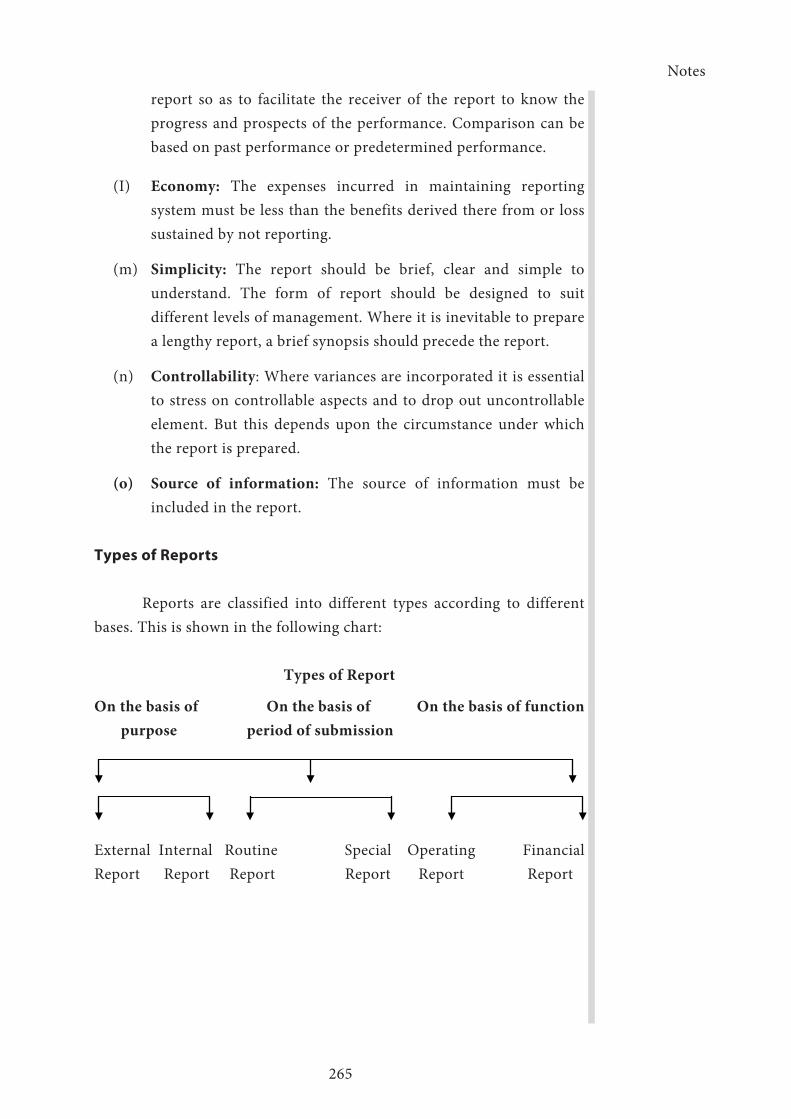
Notes

265

report so as to facilitate the receiver of the report to know the progress and prospects of the performance. Comparison can be based on past performance or predetermined performance.

(I) Economy: The expenses incurred in maintaining reporting system must be less than the benefits derived there from or loss sustained by not reporting.

(m) Simplicity: The report should be brief, clear and simple to understand. The form of report should be designed to suit different levels of management. Where it is inevitable to prepare a lengthy report, a brief synopsis should precede the report.

(n) Controllability: Where variances are incorporated it is essential to stress on controllable aspects and to drop out uncontrollable element. But this depends upon the circumstance under which the report is prepared.

(o) Source of information: The source of information must be included in the report.

Types of Reports

Reports are classified into different types according to different bases. This is shown in the following chart:

Types of Report

On the basis of On the basis of On the basis of function purpose period of submission

External Internal Routine Special Operating Financial Report Report Report Report Report Report

Notes

266

I. On the Basis of Purpose

On the basis of purpose, reports can be classified into two types, viz., (a) External report, and (b) Internal report.

(a) External report: External report is prepared for meeting the requirements of persons outside the business, such as shareholders, creditors, bankers, government, stock exchange and so on. An example of external report is the published accounts, viz., profit and loss account and balance sheet. External report is brief in size as compared to internal report and they are prepared as per the statutory requirements.

(b) Internal report: Internal report is meant for different levels of management. This can again be classified into three types: (a) Report meant for top level management, (b) Report meant for middle level management, and (c) Report meant for lower level management. Report to top level management should be in summary form giving an overall view of the performance of the business. Whereas external reports are prepared annually, internal reports are prepared frequently to serve the needs of management. Internal report need not conform to any standard as it is not statutorily required to be prepared.

II. On the Basis of Period of Submission

According to this basis, reports can be classified into two types, viz., (I) Routine reports, and (2) Special reports.

(a) Routine reports: They are prepared periodically to cover normal activities of the business. They are submitted to different levels of management according to a fixed time schedule. While some reports are prepared and submitted at very short intervals, some are prepared and submitted at a long interval of time. Some examples of routine reports relate to monthly profit and loss ccount, monthly balance sheets, monthly production, purchases, sales, etc.

(b) Special reports: Special reports are prepared to cover specific or special matters concerning the business. Most of the special

Notes

267

reports are prepared after investigation or survey. There is no standard form used for submitting this report. Some of the matters which are covered by special reports are: causes for production delays, labour disputes, effects of machine breakdown, problems involved in capital expenditure, make or buy problems, purchase or hire of fixed assets, price fixation problems, closing down or continuation of certain departments, cost reduction schemes, etc.

III. On the Basis of Function

According to the purpose served by the reports, it can be classified into two types, viz., -(a) operating report, and (b) financial report.

(a) Operating report: These reports are prepared to reveal the various functional results. These reports can again be classified into three types, viz., (a) Control reports, which are prepared to exercise control over various operation of the business, (b) Information report, which are prepared for facilitating planning and policy formulation in a business, (c) Venture measurement report which is prepared to show the result of a specific venture undertaken as for example a new product line introduced.

(b) Financial report: Such reports provide information about financial position of the undertaking. These reports may be prepared annually to show the financial position for the year as in the case of balance sheet or periodically to show the cash position for a given period as in the case of fund flow analysis and cash flow analysis.

The following list briefly defines several other types of reports.

1. Physical Description Report

Physical description reports describe the physical characteristics of a machine, a device, or some other type of object. They also explain the relationship of one part of the object to other parts so that the reader can visualize the object as a unit. Physical description reports are many times combined with process, analysis, or investigation reports.

Notes

268

2. Process Report

Process reports explain how products are produced, tests are completed, or devices operate by describing the details of procedures used to perform a series of operations. Process reports may be general or detailed. General process reports are addressed to persons not directly involved in performing the process. Detailed process reports are designed to give the readers all the necessary information needed to complete the process.

3. Analytical Report

Analytical reports critically examine one or more items, activities, or options. They are structured around an analysis of component parts or other common basis for comparison between options. This type of report usually results in conclusions and recommendations.

4. Examination Report

Examination reports are used to report or record data obtained from an examination of an item or conditions. Examination reports differ from one another in subject matter and length. Some are similar to analytical reports but are less complicated because the information is obtained from personal observations.

Examination reports are logically organized records investigating topics such as accidents or disasters. They are usually prepared for people knowledgeable about the subject and not for the general reader.

5. Laboratory Report

Laboratory reports record and communicate the procedures and results of laboratory activities. Equipment, procedures, findings, and conclusions are clearly presented at a level appropriate for readers with some expertise in the subject. They are sometimes presented in laboratory notebooks using neatly handwritten text and charts.

Notes

269

6. Literature Review

Literature reviews are logically organized summaries of the literature on a given subject. It is important that they are correctly documented and accurately represent the scope and balance of the available literature.

Conclusions drawn reflect the collection as a whole and should appropriately reflect various points of view. Overuse of direct quotations should be avoided.

7. Design Portfolio

Design portfolios are organized presentations of preliminary and final designs of items such as mechanisms, products, and works of art. When part of an educational activity, they may also include an analysis of the problem, review of related designs, evaluation, and other information. The presentation may be in the form of notes, sketches, and presentation illustrations.

8. Detail Report

Detail Report: Prints a text report outlining each audit question as well as the scoring criteria and responses entered for each question. Compliance level is calculated as a percentage at the end of the report.

9. Graphical Report (points)

Compares your possible score (in compliance points) to your actual score in a bar graph format. Then calculates your compliance score as a percentage and sorted by audit section number.

10. Graphical Report (%)

Compares your possible score (percentage) to your actual score in a bar graph format.

11. Non-Compliance Report

Prints a listing of the audit questions on which you failed to reach

Notes

270

compliance. Includes the audit section number for each question and the actual score vs. possible score.

12. Non-Compliance Graphical Report

Prints a bar graph report of those audit questions on which you failed to reach compliance.

13. Summary Report

A report allowing users to summarize responses based on the selection from four fields.

14. Trend Report

A report allowing users to view trends over a defined time frame.Management Reporting

A research report can be classified into decision-oriented (technical) report and research - oriented report. Further, the research-oriented report can be classified into survey-based research report and algorithmic research report.

1 Decision-Oriented (Technical) Report

The steps of preparing decision-oriented report are presented below:

i. Identification of the problem

ii. Establishment objectives

iii. Generation of decision alternatives

iv. Evaluation of decision alternatives

v. Selection of the best decision alternative

vi. Development of action plan

vii. Provision for correction plan after implementation of the decision.

Notes

271

2. Survey-Based Research Report

The main body of the report for the survey-based research contains the following:

i. Problem definition

ii. Objectives of the research

iii. Research methodology

iv. Data analysis

v. Interpretation of results and suggestion

vi. Conclusions.

3. Algorithmic Research Report

There are problems, viz., production scheduling, JIT, supply chain management, line balancing, layout design, portfolio management, etc., exist in reality. The solution for each of the above problems can be obtained through algorithms. So, the researchers should come out with newer algorithms or improved algorithms for such problems. For a combinatorial problem, the researcher should attempt to develop an efficient heuristic. The algorithmic research report can be classified into the following categories:

1. Algorithmic research report for combinatorial problem

2. Exact algorithmic research report for polynomial problem.

Algorithmic research report with modeling for combinatorial problem

The main body of this type of research report will contain the following:

i. Problem identification

ii. Literature review

iii. Objectives of the research

iv. Development of mathematical model

v. Design of algorithm (heuristic)

vi. Experimentation and comparison of the algorithm with the model

Notes

272

in terms of solution accuracy

vii. Experimentation and comparison of the algorithm with the best existing algorithm (heuristic) in terms of solution accuracy

viii. Case study

ix. Conclusions.

In this type of research, the results of the algorithm will be compared with the optimal results of the mathematical model as well as with the results of the best existing algorithm to check its solution accuracy through a carefully designed experiment

Note: In a research related to combinatorial problems in new and complex area, development of a mathematical model to obtain the optimal solution may not be easy.

Under such situation, the results of the algorithm (heuristic) should be compared with that of the best w existing heuristic alone for checking its solution accuracy through a carefully designed experiment

Exact algorithmic research report for polynomial problem

The main body of this type of research report will contain the following:

i. Problem identification

ii. Literature review

iii. Objectives of the research

iv. Design of exact algorithm

v. Experimentation arid comparison of the exact algorithm with the best existing exact algorithm in terms of computational time

vi. Case study

vii. Conclusions.

In a research related to polynomial problem, the researcher will have to develop an efficient exact algorithm in terms of computational time and compare it with the best existing exact algorithm for that problem through a carefully designed experiment. The comparison in terms of solution accuracy does not apply here because all exact algorithms will give optimal solution.

Notes

273

Forms of Report

Reporting of information management takes different forms. They are explained below:

1. Oral Report

An oral report is not very popular as it does not serve any evidence and cannot be referred to in future. Oral report may take the form of a meeting with individuals or a conference.

2. Descriptive Reports

These are written in narrative style. They are frequently supported by tables and charts to illustrate certain points covered in the report. One important point that must be considered in drafting this form of report is the language. The language used must be simple, easy to understand and lucid. Where the report is very long, it must be suitably divided into paragraphs with headings. They must cover all the principles of.good report discussed earlier.

3. Comparative Statement

This form of report is used for preparing the routine report. Under this method the particulars of information are shown in a comparative form, i.e., the actual results an compared with planned results and the deviations between the two arc indicated. The various tools used to prepare this form of report arc comparative financial statements, ratio analysis, fund flow analysis and so on.

4. Diagrammatic and Graphic Representation

This is more popular form of preparing reports. They occupy lesser space and give at a glance the whole picture about a particular aspect of study. They also facilitate in comparative study and show the trend over a period of time. This form of report can be used where a report contains presentation of statistical numbers and other facts and figures it overcomes the language barrier and is very easily understood by everyone.

Notes

274

Of course when large numbers are involved, it is to be reduced by selecting a convenient scale Diagrammatic representation involves the following forms:

(a) Bar diagram: it was horizontal and vertical axes to show the magnitude of values, quantity and period. Bar diagrams are of the following types.

(i) Simple bar diagram: These are most popularly used in preparing reports. The consider only length but not the width to indicate the change. In formation relating to volume of production, cost of production sales, etc. for different years can be shown under this form.

(ii) Multiple bar diagram: This type of diagram is used to report related matters such as production and sales, sales and profit, advertisement and sales and so on.

(iii) Sub-divided bar diagram: This form of diagram is used to report matters which involved different component parts as for example, the components of total cost of production such as prime cost, factory cost, office cost, cost,of sales.

(iv) Percentage bar diagrams: These diagrams depict the information on a percentage basis.

(b) Pie-diagram: They take the form of circles instead of bars. They facilitate comparison besides depicting the actual information under review.

5. Break-Even Chart

This type of chart is prepared to show the relationship between variable and fixed cost and sales. It shows the point of no-profit and no-loss or where total cost equals to total revenue received.

6. Gantt Chart

This chart was first introduced by Heny L. Gantt. It is a special type of bar diagram under which bars are drawn horizontally. This chart shows

Notes

275

the bars of planned schedule and attained performance. They are largely used to denote utilization of machine capacity.

Reports Submitted to Various Levels of Management

1. Top Level Management

The top level management comprises of board of directors, managing director, and other executives who are concerned with determination of objectives and formulation of policies. Top management is to be furnished with reports at regular intervals in order to enable them to exercise control over the activities of the business. The following are some of the reports submitted to board of directors.

a) Master budget which covers all functional budgets for taking remedial actions where there are significant deviations from budgeted figures.

b) Various functional budgets prepared by various departmental managers for holding departmental managers for any shortfall in their performance.

c) Capital expenditure budget and cash budget to know the extent of variances for taking remedial measures.

d) Reports relating to production and sales, which shows the trend of the performance of business.

e) Report covering important ratios such as stock turnover ratio, fixed assets turnover ratio, liquidity ratio, solvency ratio, profitability ratios, etc. to know the improvement in business.

f) Appraisal of various projects undertaken by the organization.

2. Middle Level Management

It comprises of different departmental managers such as production manager, purchase manager, sales manager, chief accountant, etc. These managers require reports to improve the efficiency of their respective departments. The following are some of the matters reported to production manager:

Notes

276

(a) Report relating to actual capacity utilized as compared to budgeted capacity.

(b) Report relating to actual output as against standard output.

(c) Labour and machine capacity utilized.

(d) Idle time lost.

(e) Report on scraps, wastages and losses in production.

(/) Report relating to stock of raw materials, work-in-progress and finished goods.

(g) Report relating to cost of production, operation of different departments.

The following are some of the matters reported to sales manager:

(a) Report relating to number of orders executed, orders received and orders on hand.

(b) Reports relating to actual sales and budgeted sales and actual selling and distribution expenses and budgeted selling and distribution expenses.

(c) Summary of selling expenses incurred in different territories and their corresponding sales.

(d) Gross profit earned on different products and in different areas.

(e) Market survey reports.

(/) Report relating to present and potential demand.

The following are some of the matters reported to financial manager:

(a) Report relating to cash position.

(b) Summary of receipts and payments.

(c) Report relating to outstanding debts on credit sales.

(d) Report on debts due on credit purchases.

(e) Monthly profit and loss account.

(f) Quarterly report on capital expenditure.

Notes

277

3. Lower Level Management

The lower level management includes supervisors, foremen and inspectors who are concerned with the operations of the factory. They are interested in increasing the efficiency of the production departments. The reports that are to be sent to them are variances relating to planned and actual performance. The report must also emphasize cost control aspects.

Management Reporting Requirements

(a) General

This document prescribes management reports required if the offer requests progress payments and a progress payments clause is included in the subcontract. They are in addition to technical reports required under the subcontract, but must be consistent with data furnished under those requirements. Preferred formats for the Billing Plan/Management Report and the Milestone Schedule and Status Report are attached.

(b) Description of Reports

(1) Billing Plan/Management Report, Form

This report shows the planned rate of progress payment billings and billings for accepted supplies under each major task for the remainder of the subcontract performance period. For each task, the planned billings are to be projected in monthly increments for each of the twelve months of the current or succeeding fiscal year, and in fiscal year increments thereafter for the remainder of the subcontract. (Projected billings should be directly related to the activities scheduled to be performed during each billing period, as reflected on the Milestone Schedule and Status Report.) or schedule. Each time it is necessary to alter the plan, a new plan and narrative explanation for the change will be provided to the Company.

(B) As a monthly report, this document provides a comparison of the planned billings with the actual billings for work performed as of the cut-off period for the report. Variances from the plan are computed, and explanations for variances exceeding + 10% will be provided by the Seller in the Narrative Highlights Report.

Notes

278

In addition, upon the occurrence of a variance exceeding + 10%, the Seller must reevaluate the estimated billings for the balance of the current fiscal year and to the completion of the subcontract. Narrative explanations must be provided for significant changes to these estimated billings.

(2) Milestone Schedule and Status Report

This is used both as a baseline plan and status report.

As a baseline plan, it establishes the Seller’s schedule for accomplishing the planned events and milestones of each reporting category identified in the subcontract.

As a status report, it measures status or progress against the baseline plan. It will reflect planned and accomplished events, milestones, slippages, and changes in schedule.

(3) Narrative Highlights Report

The Narrative Highlights Report permits management presentation of the technical aspects of subcontract performance along with an overview of significant project highlights, accomplishments, and problems. The report will continue discussions of items identified in the previous report through completion of an activity or resolution of a problem. Typical reporting elements to be covered by brief statements are:

(A) Major accomplishments and significant highlights.

(B) Major subcontract awards, including award date, subcontract amount, and scheduled completion date.

(C) Developments affecting estimates and schedules. This will specifically include explanations of deviations from the Billing Plan which exceed + 10% and deviations from Milestone Schedule Plan which exceed 30 days.

(D) Revised estimates or schedules.

(E) Technical problems encountered and resolution actions proposed.

(F) Planned major accomplishments during the next 60 days.

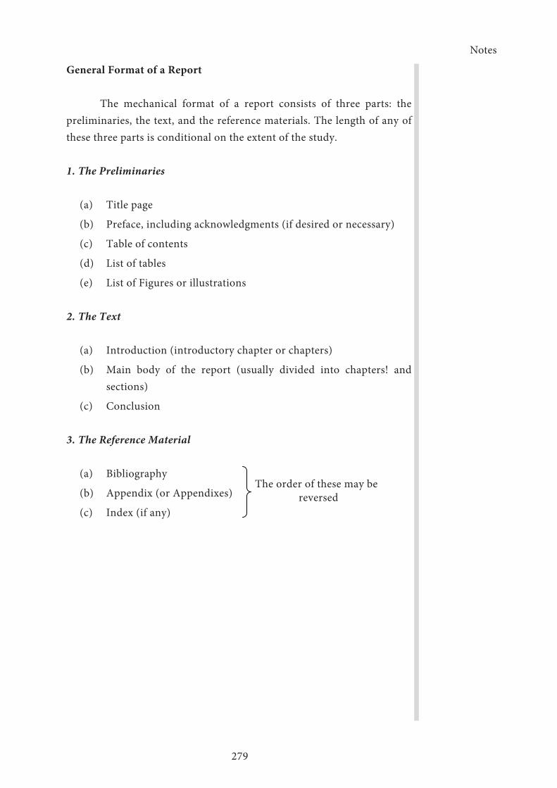
Notes

279

General Format of a Report

The mechanical format of a report consists of three parts: the preliminaries, the text, and the reference materials. The length of any of these three parts is conditional on the extent of the study.

1. The Preliminaries

(a) Title page

(b) Preface, including acknowledgments (if desired or necessary)

(c) Table of contents

(d) List of tables

(e) List of Figures or illustrations

2. The Text

(a) Introduction (introductory chapter or chapters)

(b) Main body of the report (usually divided into chapters! and sections)

(c) Conclusion

3. The Reference Material

(a) Bibliography The order of these may be

(b) Appendix (or Appendixes)

(c) Index (if any)reversed

Notes

280

The Preliminaries

1. Title Page

Generally, the following information is required:

Written Report

(a) Title of the report

(b) Name/s of the writer/s

2. Preface

The preface (often used synonymously with foreword) may include: the purpose in conducting the study, a brief background, scope, purpose, general nature of the activity/research upon which the report is being based and acknowledgments.

3. Table of Contents

The table of contents includes the major divisions of the report: the introduction, the chapters with their subsections, and the bibliography and appendix. Page numbers for each of these divisions are given. Care should be exercised that titles of chapters and captions of subdivisions within chapters correspond exactly with those included in the body of the report.

In some cases, sub-headings within chapters are not included in the table of contents. It is optional whether the title page, acknowledgments, list of tables and list of Figures are entered in the table of contents. The purpose of a table of contents is to provide an analytical overview of the material included in the study or report together with the sequence of presentation.

To this end, the relationship between major divisions and minor subdivisions needs to be shown by an appropriate use of capitalisation and indentation or by the use of a numeric system.A table of contents is necessary only in those papers where the text has been divided into chapters or several subheadings.

Notes

281

The basic criterion for the inclusion of subheadings under major chapter division is whether the procedure facilitates the reading of a report and especially the location of specific sections within a report.

4. List of Tables

After the table of contents, the writer needs to prepare a list of tables. The heading LIST OF TABLES, should be centered on a separate page by itself.

5. List of Figures (or Illustrations)

The list of Figures appears in the same form as the list of tables. The page is headed LIST OF FIGURES, without terminal punctuation, and the numbers of the Figures are listed at the left of the page under the heading Figure.

6. Introduction

An introduction should be written with considerable care: with two major aims in view: introducing the problem in a suitable context, and arousing and stimulating the reader’s interest. If introductions are dull, aimless, confused, rambling, and lacking in precision, direction and specificity; there is little incentive for the reader to continue reading. The length of an introduction varies according to the nature of the matter reported.

7. Main Body of the Report

There are certain general principles which should be followed:

(a) Organize the presentation of the argument or findings in a logical and orderly way, developing the aims stated or implied in the introduction.

(b) Substantiate arguments or findings.

(c) Be accurate in documentation.

Notes

282

8. Conclusion

The conclusion serves ‘the important function of tying together the whole gamut of the report or assignment. In summary includes, important findings discussed and conclusions drawn from the whole study. In addition, the list unanswered questions that have occurred in the course of the reporting and which require further enquiry beyond the limits of the project being reported. The conclusion should leave the reader with the impression of completeness and of positive gain.

9. Bibliography

The bibliography follows the main body of the text and is a separate but integral part of a thesis, preceded by a division sheet or introduced by a centered capitalized heading BIBLOGRAPHY. Pagination is continuous and follows the page numbers in the text. In a written assignment, the word bibliography may be a little pretentious and the heading REFERENCES may be an adequate alternative.

10. Appendix

It is usual to include in an appendix such matters as original data, tables that present supporting evidence, tests that have been constructed by the research student, parts of documents or any supportive evidence that would detract from the major line of argument and would make the body of the text unduly large and poorly structured. Each appendix should be clearly separated from the next and listed in the table of contents.

11. Index

If an index is included, it follows the bibliography and the appendix. An index is not required for a written assignment or for an unpublished thesis. If a thesis is subsequently published as a book, monograph or bulletin, an index is necessary for any or of complexity.

Notes

283

12. The Abstract

An abstract consists of the following parts

1. A short statement of the problem.

2. A brief description of the methods and procedures used in collecting the data.

3. A condensed summary of the findings of the study.

The length of the abstract may be specified, for example, 200 words. Usually an abstract is short.13. The Final Report

From the outset, the aim is, at the production of a piece of work of high quality. The text should be free of errors and untidy corrections. Paper of standard size (usually quarto) and good quality should be used for preparation of the report.

Self Assessment Questions

1. What is social cost benefit analyzed?

2. Define social cost accounting

3. What are the advantages of social cost benefit analyze

4. Explain Decision Tree in Management

5. What are the different types of report? Explain them in brief.

6. Discuss the guidelines for reviewing the draft of a report.

7. What are the qualities of a research report? Explain them in brief.

8. Give a sample cover page of a research report.

9. Discuss the items of the introductory pages in detail.

10. Give sample table of-contents of a survey based research report.

11. Give a sample table of contents of an algorithmic research report.

12. What are the items under the text of a research report? Explain them in brief.

13. Discuss the guidelines for preparing bibliography.

Notes

284

14. Give a brief account of typing/printing instructions while preparing a research report.

15. Discuss the guidelines for oral presentation of a research report

16. Assume a research topic of your choice and give the complete format of its research report

17. What do you understand by the term “reporting to management”?. Discuss briefly the matters that you would deal with while reporting to the board of directors.

18. Discuss the general principles to be observed while preparing reports.

19. Describe the various forms of reporting to management.

20. Distinguish between routine and special reports. State the various matters which are sent to management under routine and special reports

21. Explain different types of reports submitted to the management of an organisation.

22. Explain the information submitted to different levels of management.

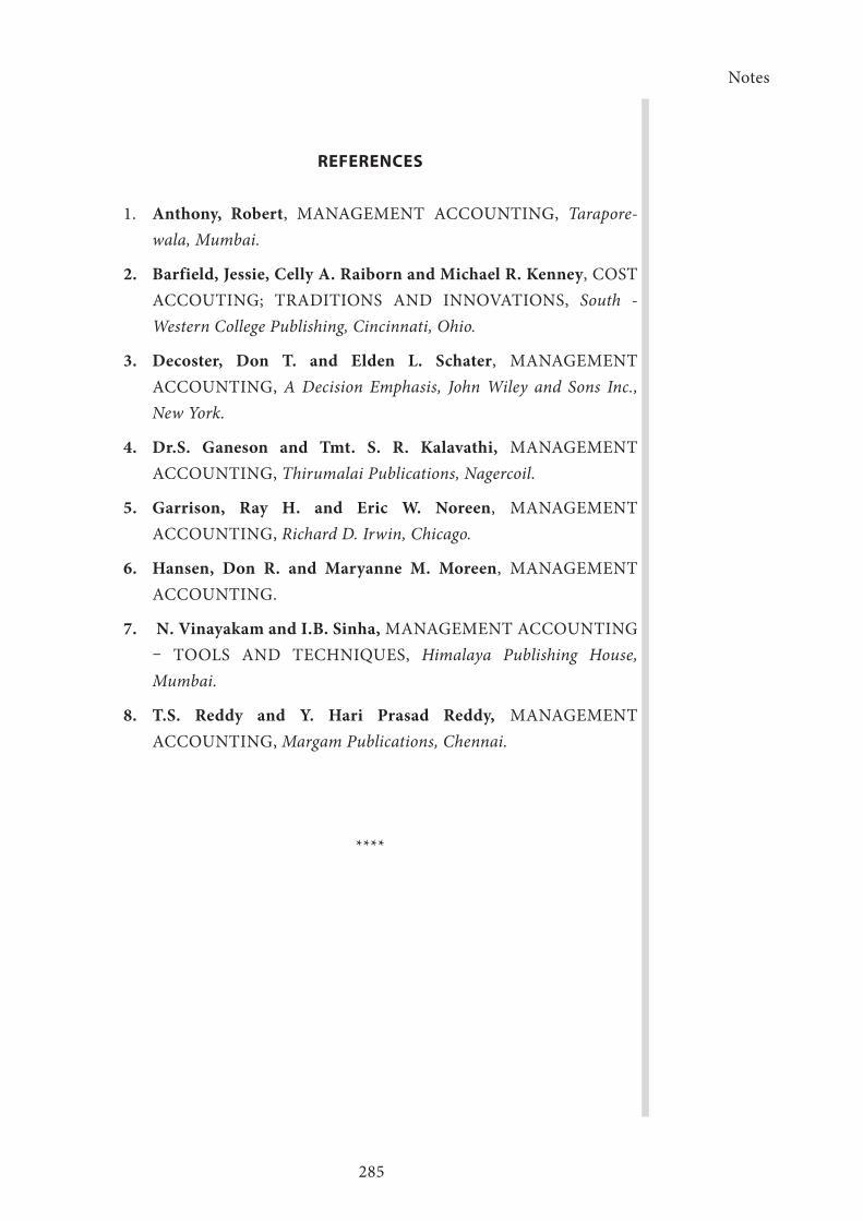
Notes

285

REFERENCES

1. Anthony, Robert, MANAGEMENT ACCOUNTING, Tarapore-wala, Mumbai.

2. Barfield, Jessie, Celly A. Raiborn and Michael R. Kenney, COST ACCOUTING; TRADITIONS AND INNOVATIONS, South - Western College Publishing, Cincinnati, Ohio.

3. Decoster, Don T. and Elden L. Schater, MANAGEMENT ACCOUNTING, A Decision Emphasis, John Wiley and Sons Inc., New York.

4. Dr.S. Ganeson and Tmt. S. R. Kalavathi, MANAGEMENT ACCOUNTING, Thirumalai Publications, Nagercoil.

5. Garrison, Ray H. and Eric W. Noreen, MANAGEMENT ACCOUNTING, Richard D. Irwin, Chicago.

6. Hansen, Don R. and Maryanne M. Moreen, MANAGEMENT ACCOUNTING.

7. N. Vinayakam and I.B. Sinha, MANAGEMENT ACCOUNTING – TOOLS AND TECHNIQUES, Himalaya Publishing House, Mumbai.

8. T.S. Reddy and Y. Hari Prasad Reddy, MANAGEMENT ACCOUNTING, Margam Publications, Chennai.

****