managed care competition - research papers in...
TRANSCRIPT
Managed Care Competition and the Adoption of Hospital
Technology: The Case of Cardiac Catheterization †
Farasat A.S. Bokhari
Department of EconomicsFlorida State University
Last Revision: July 2008
AbstractThe diffusion of health care technology is influenced by both the total market share of managed careorganizations as well as the level of competition among them. This paper differentiates between HMOpenetration and competition and examines their relationship to the adoption of cardiac catheterizationlaboratories in all non-federal, short-term general community hospitals in the U.S. between 1985 and 1995.Results show that a hospital is less likely to adopt the technology if HMO market penetration increasesbut more likely to adopt if HMO competition increases. Further, the latter effect is non-linear in thenumber of adopters. In markets where fewer than a critical number of neighboring hospitals have alreadyadopted, the probability of adoption increases with the number of HMOs, but in markets where morethan the critical number of neighbors have already adopted, the probability of adoption decreases withthe number of HMOs. Thus, in markets where technology is rare, HMO penetration and competition havecountervailing effects on the diffusion of technology such that the net effect could be small.
Key words: HMO Competition; HMO Penetration; Hospital Technology Adoption; Discrete TimeHazard Rate Model
JEL Classification: I11, O14,O39
†I greatly appreciate the comments and feedback provided by Martin Gaynor, Ashish Arora, William Vogt, Gary Fournier,Rick Smith, Nadine Zubair, Jonah Gelbach, Frank Heiland and seminar participants in the Health Policy Research TrainingProgram (2001-2003) at the University of California at Berkeley’s School of Public Health. The usual caveats apply.
Email address: [email protected]; TEL (850) 644-7098 (Farasat A.S. Bokhari).
Managed Care Competition 1
1. Introduction
How does the change in competition among health maintenance organizations (HMOs) affect dif-
fusion of technology among hospitals? Changes in health care technologies have often been cited
as the main reason for rising health care costs (Newhouse, 1992). Managed care organizations, or
HMOs more specifically, are believed to be the market based response to the earlier cost-plus reim-
bursement mechanisms that lead to excessive investment in technologies by competing hospitals.1
Having more patients insured under HMO contracts enhances the bargaining power of third party
payers and acts as a countervailing power against the excesses of hospital competition. However,
the empirical case for managed care as a check on the medical arms race (MAR) is weak and
with mixed results. In particular, the literature blurs the distinction between the growth of HMO
penetration, i.e., with more members, the HMOs enjoy stronger bargaining power in negotiation
rates with hospitals, and the effect of competition among HMOs. More recently, the managed care
industry is being transformed and HMOs are themselves facing intense local competition (the aver-
age number of HMOs per market increased from 4.6 to 9.9 between 1985 and 1995). With greater
number of HMOs to choose from, the impetus for reining in the MAR may be lost as HMOs vie for
patients along price and non-price competition by offering access to more technology rich hospitals.
The opposing effects of penetration and competition among HMOs, and their implications for the
diffusion of technologies in hospitals is the focus of this paper.
The HMO-hospital relationship differs from typical vertical relations in that HMOs intermediate
competing platforms with network externalities that patients and hospitals choose. Specifically, in
the standard language of platforms and two-sided markets, enrollees and hospitals form the two
sides, and the HMO is an intermediary firm that offers a menu of health care plans (platforms).
The intermediary firm (HMO) charges a different price on each side of the market – a positive price
to enrollees (a premium) and a negative price to the hospitals (a payment for services). Further,
the enrollees enjoy a higher utility if the HMO contracts with more hospitals with the technology
(a network externality for the enrollees) while the hospitals obtain larger total revenue (from the
HMO) if the contracting HMO has more enrollees. Thus, the platform provider’s problem is to
offer either only a single plan to all enrollees, or to offer differentiated (two) plans and let the
enrollees self-select into a higher premium plan with access to all hospitals in the network with
the technology and a lower premium plan with restricted access to hospitals with technology. In
the current context, the emergence of multiple plans implies that HMOs rationalize the adoption
1An HMO plan entails a capitation payment to providers and where the enrollees are assigned a primary care physician(PCP) who may then refer them for further treatment to a preselected group of providers (hospitals or specialists). Thus, theHMO need not be a vertically integrated insurance and service provider firm. There is a large variety of different types ofmanaged care organizations (MCOs), consisting of HMOs, Preferred Provider Organizations (PPOs), Independent PracticeAssociations (IPAs) etc. Even though the term HMO has become almost synonymous with any type of MCO, I stick to theterm HMO since good quality and geographically detailed data over the study period is available only for HMOs and thesewere the most prevalent form of managed care activity during the study time period.
2 Adoption of Hospital Technology
of technology by hospitals rather than discourage the adoption by all hospitals as implied by the
literature on HMO penetration.
For instance, a result established by Ambrus and Argenziano (2006, p. 11-12) is that in the presence
of heterogeneous consumers, a monopolist platform provider (HMO) will always choose to setup two
asymmetric platforms, one larger and cheaper on one side of the market (low premium and many
enrollees) and the other larger and cheaper on the other side of the market (smaller discounts from
many hospitals) as long as the incremental utilities resulting from a given increase in the number
of consumers on the opposite side are uniformly bounded by a positive constant. This requirement
is met if consumers have a diminishing marginal positive value in the choice of service providers.2
Hence, in HMO monopoly markets, the HMO offer’s differentiated products and contracts with
both, hospitals with the technology as well as those without it, precisely because those that have
not yet adopted, offer a greater value to the platform provider by not adopting the technology. By
contrast, in the HMO duopoly markets, one HMO’s network is larger and cheaper for the enrollees
while the other HMO’s network is larger and cheaper for the hospitals. Thus, the effect of HMO
competition on technology adoption can be understood as an application of the effect of the number
of platform providers on the emergence of multiple platforms, i.e., hospitals with and without the
technology (for more examples, see Ambrus and Argenziano (2006)).
Baker (2001) and Baker and Phibbs (2002) have argued that managed care organizations have an
elastic demand and they are able to bargain aggressively and obtain a lower price per service for
their enrollees. Thus, as HMO penetration increases, the expected profitability of the high marginal
cost technology decreases for the price discriminating hospitals, which in turn delays the adoption
of that technology. Consistent with their explanation, I find that the probability of adoption of
cardiac catheterization laboratories (cathlabs) decreases with HMO penetration. However, I also
find that the probability of adoption may either increase or decrease with the number of HMOs,
depending on whether less or more than a critical number of neighboring hospitals have already
adopted the cathlabs. Thus, the combined effect of HMO competition and penetration could be
ambiguous (and small) since each has a countervailing effect on the adoption of technology, at least
in the early stages of adoption.
I explain the threshold effect in the HMO competition on technology adoption by extending Sorensen’s
(2003) bargaining model between HMOs and hospitals. HMOs solicit bids from hospitals and con-
tract with the lowest bidder. The equilibrium discount offered by a bidding hospital is a decreasing
2By diminishing marginal value of choice I mean the following: Holding price (premium) and other things constant,consumers prefer to enroll in HMOs that provide access to more hospitals (with technology) but this effect diminishes if eachHMO contracts with a sufficiently large number of hospitals. As an example, consider the following: If there are two HMOsand two hospitals in a market, and one HMO contracts with only one hospital and the other HMO contracts with both thehospitals, then the HMO with more contracts will steal all (or most of) the enrollees from the competing HMO. However, ina market with ten hospitals and two HMOs, if one HMO has contracts with all ten hospitals and the other has contracts withonly nine hospitals, it is no longer true that the HMO with only nine contracts will have no (or very few) enrollees.
Managed Care Competition 3
function of the number of other pre-existing hospitals in the HMOs’ network and an increasing
function of the HMOs’ ability to channel enrollees to network hospitals (henceforth, the number of
hospitals in an HMO’s network is referred to as the size of the network). In turn, an HMO’s ability
to prevent enrollees from using non-network hospitals increases if it has more network hospitals.
Thus, changing the size of the pre-existing network creates a trade-off in the discount offered by
the bidding hospitals: A bidding hospital would offer a larger discount if the size of the pre-existing
network is small, but a smaller pre-existing network also implies that an HMO’s ability to channel
enrollees to in-network hospitals is weak and hence the discount may not be large. Whether hos-
pitals offer a small or large discount depends on the relative values of the size of the pre-existing
network and the HMOs ability to prevent leakage from the network. Finally, as HMO competition
intensifies, HMOs’ offer greater choice to enrollees by offering access to larger networks of hospitals.
Consequently, the discount offered by bidding hospitals decreases (increases) with the number of
HMOs if the size of the network is less than (greater than) a threshold. Intuitively, if the existing
network is small, then hospitals offer decreasing discounts in the number of HMOs because the
bidding hospital loses a larger fraction of HMO enrollees to other network hospitals relative to the
gain that comes with more enrollees using network hospitals.
Since the discount offered by a hospital changes its expected profitability, and hence the timing of
adoption of expensive technologies, I estimate a reduced form hazard rate model for the adoption
of cathlabs in U.S. hospitals.3 The next section briefly reviews some relevant studies on HMO
penetration and technology adoption and extends the discussion to the role of HMO competition.
Section 3 specifies the empirical model and Section 4 has the results. This is followed by a brief
section on marginal probabilities as a function of the number of HMOs. The final section provides
a discussion and summary of the results.
2. Hospitals’ Adoption Decision and the Role of HMOs
2.1. Prior Literature on Adoption. There is a substantial literature that has focused on market
structure – specifically hospital competition – and technology adoption. Rapoport (1978) found
that hospitals in more competitive markets tended to adopt new innovations faster, while Luft et
al. (1986) found that a hospital is more likely to offer a specialized service if other hospitals in
the market also offer a similar service (at least for some services). Dranove et al. (1992) report
similar results but find that the MAR effect is economically small and can be explained by more
conventional factors such as the extent of the market. Hamilton and McManus (2005) investigate
the diffusion of a new injection technology (intracytoplasmic sperm) in fertility clinics and report
that clinics in competitive markets offered the technology earlier than in monopolies. Others have
3For a link between a firm’s expected profitability from adoption at time t and the hazard rate models, see Rose and Joskow(1990) or Reinganum (1989).
4 Adoption of Hospital Technology
focused on strategic interactions on the timing of adoption.4 For instance, Vogt (1998) investigates
the adoption of MRI in duopoly hospital markets and finds evidence consistent with preemptive
adoption models while Schmidt-Dengler (2006), who also studies the adoption of MRIs in small
hospital markets, finds that business-stealing effect is relatively more important than preemption.5
2.2. Literature on Adoption and HMOs. Related literature has focused on the role of insurance
on technology diffusion. Baumgardner (1991) links the changes in marginal valuation (to consumers)
of the introduction of a technology (in a hospital) to the type of insurance contract. On the basis
of this assumption he provides testable specifications that the probability a hospital will adopt an
innovation will depend upon the fraction of customers covered by an HMO versus a traditional
fee-for-service (FFS) contract. Similarly Baker and Brown (1999) provide a model that predicts the
change in the equilibrium number of (single service) health providers with changes in HMO activity.6
Both of these models suggest that at least for some technologies, an increase in HMO penetration
will discourage technology adoption by hospitals. Consistent with these predictions, Cutler and
McClellan (1996) found that hospitals in areas with high HMO enrollment are less likely to adopt
angioplasty. Similarly, Baker (2001) and Baker and Phibbs (2002) estimate models for the adoption
of magnetic resonance imaging and neonatal intensive care units respectively and find that in both
cases the increases in HMO penetration are associated with a decrease in the adoption hazard.
However, Baker and Spetz (1999) investigate several technologies and report mixed findings.
Baker and Phibbs (2002) argue that managed care organizations have the ability to change both the
price and volume of services provided by hospitals, which in turn change the expected profitability
of these services and hence the time to adoption (the implicit assumption is that a hospital will
adopt a new technology when the discounted expected profit at a given time from adopting the
technology is greater than from not adopting it). In the former case they argue that because
managed care organizations have an elastic demand, they bargain aggressively and obtain a lower
price per service for their enrollees. Thus, if the number of managed care enrollees increases, the
expected profitability of the high marginal cost technology decreases for the price discriminating
hospitals, which in turn delays the adoption of that technology. In the latter case they argue that
managed care organizations also affect the adoption decision via influencing the total volume: Since
managed care organizations limit the use of expensive (high marginal cost technologies) for their
enrollees, they may influence the practicing/prescribing behavior of the in-network physicians such
4Often these papers test assumptions or predictions of theoretical models of adoption in the IO literature, e.g. Reinganum(1981); Fudenberg and Tirole (1985).
5There is also a large literature on regulations (e.g CON laws, introduction of PPS) and adoption of technology and is notreviewed here. See Acemoglu and Finkelstein (2006); Sloan et al. (1988); Joskow (1981); Sloan and Steinwald (1980); Salkeverand Bice (1976).
6However, they also predict that the number of providers will increase with an increase in HMO activity for services thatare preferred by managed care compared to traditional insurance as long as the loss in profits from increased HMO penetrationis smaller than the gain in profitability from knowledge spill-overs and market expansion.
Managed Care Competition 5
that there is a reduction in the volume of services even by the FFS patients of these physicians.
Further, competitive pressures felt by traditional FFS insurance companies may also force them
to bring changes in the services they cover. This too implies a reduction in expected profitability
which may further delay the adoption of technologies.
However, in all of the papers cited above, an increase in managed care activity is synonymous
with an increase in managed care penetration (i.e. percent of population enrolled in managed
care plans) and does not accounting for competition among managed care organizations. Pauly
(1998) has argued that concentration in the insurance market can lead to more price competition in
hospital markets. It is important to recognize that penetration and competition (within managed
care firms) are not two faces of the same coin, and could have very different effects on hospital
profitability vis-a-vis their relative bargaining power with the hospitals. More generally, the mixed
results on the effect of HMO penetration on technology adoption (see Baker and Spetz (1999))
could be due to the omission of HMO competition or their relative bargaining power. For instance,
Gaynor and Haas-Wilson (1999) note that the merger wave of 1990s, both among the providers and
insurers, was in part driven by attempts to strengthen their bargaining positions. In this paper, I
explicitly recognize the competition effect (as separate from the penetration effect) and show that
HMO penetration and competition have opposite effects on adoption decisions by hospitals when
there are few hospitals with the technology. Consistent with my results, Shen et al. (2008) find
that HMO penetration and concentration have distinct effects on hospital revenue per patient, but
more importantly, hospital revenue growth is slower in markets where HMOs are concentrated but
hospitals are competitive.
2.3. Extension to the Number of HMOs. The effects of HMO competition on the price and
volume of services provided by hospitals follow naturally from this literature. The basic intuition is
that when there are multiple HMOs in an area, then no one HMO may have substantial bargaining
power to obtain large discounts from hospitals.
2.3.1. Price. Consider the price effect. Since HMOs’ demand is elastic (Welch, 1986) and they
bargain with providers for a lower price per service for their enrollees, a given HMO can do this
effectively if it has a relatively large market share of the HMO market. If, on the other hand, the
number of HMOs is also relatively large, such that each individual HMO has only a very small share
of the market, then getting large price discounts from the hospitals may not be possible. This would
be true even if an individual HMO’s threat to channel patients to alternative hospitals is credible
since the total enrollment of the HMO is small. Thus, while the threat is credible, it is ineffectual.
This in turn implies that for a hospital facing a given level of aggregate HMO penetration, expected
discounted profits from the adoption of a technology are likely to be higher if the HMO enrollees
6 Adoption of Hospital Technology
are distributed across many firms than when the HMO market is dominated by only a handful of
firms.
2.3.2. Volume. Changes in the number of HMOs can change the hospitals’ expected discounted
profits via changes in volume of services provided by hospitals. While each HMO may use mecha-
nisms to induce network physicians to lower the use of expensive technologies, their ability to do so
may be limited if there are many HMOs competing with each other to sign enrollees and physicians
into their network. If the number of HMOs increases, it may induce greater non-price competition
among them. In order to attract physicians and patients, they would be under greater pressure
to relax utilization reviews and other mechanisms by which they control the volume of services
provided by hospitals and physicians. Ceteris paribus, the expected profitability for a hospital from
the adoption of an expensive technology at a given time will be greater if there are more HMOs in
the market than if there were a few. Additionally, there may be a very limited, or even no change
in the prescribing behavior of the network physicians implying a lack of reduction of volume even
among the FFS patients seen by the same physicians.
2.3.3. Non-linearities. HMOs compete with each other for enrollees by offering lower premiums
and/or access to more service providers with technology. It is possible that the impact of the number
of HMOs on the adoption of technology by hospitals will be non-linear (or more accurately, have a
threshold effect): If fewer than a critical number have adopted that technology, then the probability
of adoption will increase with the number of HMOs but once it is relatively well diffused (more than
a critical number have adopted) the probability will decrease with more HMOs. I describe below
one specific model from the literature, which, with some modifications, generates this non-linearity7.
Sorensen (2003) describes a simple bargaining model with one HMO and two perfect substitute
hospitals where the HMO’s enrollees are expected to require S units of hospital service and the
HMO solicits bids from two hospitals. He shows that the symmetric equilibrium bidding strategy of
each hospital is d∗i = (1− ci)(1− (1/2γ)) where the price of a unit of hospital service is normalized
to 1 and where di and ci is the discount offered by hospital i and its unit cost respectively (where
ci ∈ [0, 1]). In his model, a parameter γ (where 1/2 ≤ γ ≤ 1), is exogenous and is the degree to
which the insurer can channel its patients to a given hospital (γ = 1/2 means that the HMO has no
ability to do so and 1 means that it has full control). Thus γ is the ability of the HMO to restrict
patients to the network hospital which provides γS units of service at the unit price of 1− di while
the non-network hospital provides (1− γ)S units of service at the full price of 1.
7Note, this is not the only model that can generate such a non-linearity. The purpose is to provide an economic frameworkand context to help understand the empirical results that follow.
Managed Care Competition 7
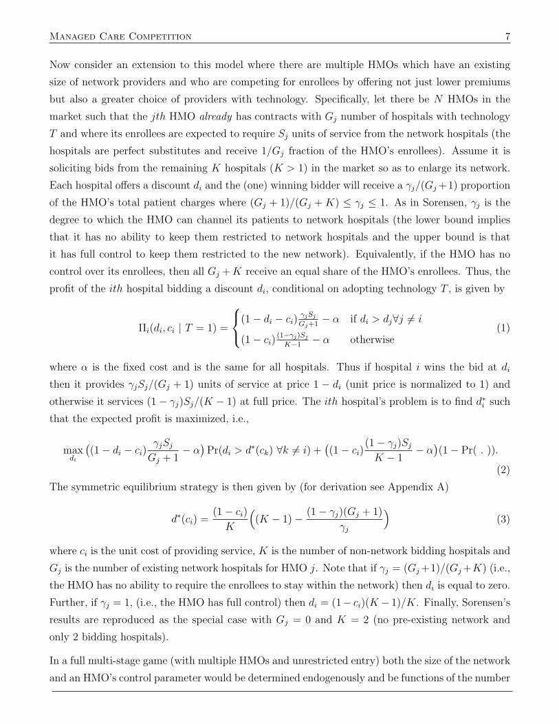
Now consider an extension to this model where there are multiple HMOs which have an existing
size of network providers and who are competing for enrollees by offering not just lower premiums
but also a greater choice of providers with technology. Specifically, let there be N HMOs in the
market such that the jth HMO already has contracts with Gj number of hospitals with technology
T and where its enrollees are expected to require Sj units of service from the network hospitals (the
hospitals are perfect substitutes and receive 1/Gj fraction of the HMO’s enrollees). Assume it is
soliciting bids from the remaining K hospitals (K > 1) in the market so as to enlarge its network.
Each hospital offers a discount di and the (one) winning bidder will receive a γj/(Gj +1) proportion
of the HMO’s total patient charges where (Gj + 1)/(Gj + K) ≤ γj ≤ 1. As in Sorensen, γj is the
degree to which the HMO can channel its patients to network hospitals (the lower bound implies
that it has no ability to keep them restricted to network hospitals and the upper bound is that
it has full control to keep them restricted to the new network). Equivalently, if the HMO has no
control over its enrollees, then all Gj +K receive an equal share of the HMO’s enrollees. Thus, the
profit of the ith hospital bidding a discount di, conditional on adopting technology T , is given by
Πi(di, ci | T = 1) =
(1− di − ci) γjSjGj+1
− α if di > dj∀j 6= i
(1− ci) (1−γj)SjK−1
− α otherwise(1)
where α is the fixed cost and is the same for all hospitals. Thus if hospital i wins the bid at di
then it provides γjSj/(Gj + 1) units of service at price 1 − di (unit price is normalized to 1) and
otherwise it services (1− γj)Sj/(K − 1) at full price. The ith hospital’s problem is to find d∗i such
that the expected profit is maximized, i.e.,
maxdi
((1− di − ci)
γjSjGj + 1
− α)
Pr(di > d∗(ck) ∀k 6= i) +((1− ci)
(1− γj)SjK − 1
− α)(1− Pr( . )).
(2)
The symmetric equilibrium strategy is then given by (for derivation see Appendix A)
d∗(ci) =(1− ci)K
((K − 1)− (1− γj)(Gj + 1)
γj
)(3)
where ci is the unit cost of providing service, K is the number of non-network bidding hospitals and
Gj is the number of existing network hospitals for HMO j. Note that if γj = (Gj+1)/(Gj+K) (i.e.,
the HMO has no ability to require the enrollees to stay within the network) then di is equal to zero.
Further, if γj = 1, (i.e., the HMO has full control) then di = (1− ci)(K − 1)/K. Finally, Sorensen’s
results are reproduced as the special case with Gj = 0 and K = 2 (no pre-existing network and
only 2 bidding hospitals).
In a full multi-stage game (with multiple HMOs and unrestricted entry) both the size of the network
and an HMO’s control parameter would be determined endogenously and be functions of the number

8 Adoption of Hospital Technology
of HMOs (i.e., Gj = Gj(N) and γj = γj(Gj(N), N))8. In the absence of such a model, it is still
useful to explore (via comparative statics) the implied effect of changes in the number of HMOs on
the optimal bid. Thus, taking the derivative of d∗i with respect to N gives
dd∗idN
= −(1− ci)K
[(−1)
(Gj + 1)
γ2
{∂γj∂N
+∂γj∂Gj
∂Gj
∂N
}+( 1
γj− 1)∂Gj
∂N
], (4)
where the quantity in the curly braces ({·}) is the total or net change in the HMO’s ability to
control enrollees due to a change in the number of HMOs and is the sum of the direct effect on the
control parameter of an increase in HMOs (∂γj/∂N) and an indirect effect ((∂γj/∂Gj)(∂Gj/∂N))
due to the intermediate change in the size of the network (∂Gj/∂N). Henceforth, let the sum, i.e.,
the total effect on the control parameter, be denoted by dγj/dN .
The partials in (4) above determine the change in the optimal discount as a function of the number
of HMOs. Thus, it is necessary to make some plausible assumptions about the signs of these
partials. First, suppose that as the number of HMOs increases, the size of their network also
increases since enrollees value greater choice of service providers, i.e., ∂Gj/∂N > 0. Indeed, Capps
et al. (2003) provide a model of HMO competition, where (in the limiting case of p = mc for each
HMO), the dominant strategy for each HMO is to contract with all hospitals in the area as service
providers. Second, ∂γj/∂Gj > 0, i.e., an HMO’s control over enrollees use of network hospitals is an
increasing function of the number of hospitals in the network. Recall that γj is the fraction of the
enrollees that use network hospitals, thus this assumption is stating that if the size of the network
increases, a greater fraction would use network hospitals. In fact, in the limit that Gj increases
to all existing hospitals in the market then γj increases to its maximum value of 1. Finally, it
maybe reasonable to assume that the direct effect on the control parameter maybe decreasing in
the number of HMOs i.e., ∂γj/∂N < 0, – ceteris paribus an increase in the number of HMOs implies
a toughness of competition among them such that more of their enrollees enjoy the freedom to seek
services outside of the network.
With these three assumptions in place, note that the indirect effect of an increase in HMOs on the
HMO control parameter is positive ((∂γj/∂Gj)(∂Gj/∂N) > 0) while the direct effect on the HMO
control parameter is negative (∂γj/∂N < 0). If the direct effect is larger, so that the total effect
(sum of the two) is negative then the entire quantity in the square brackets in (4) is unambiguously
positive and hence dd∗i /dN < 0. Put another way, if the number of HMOs increases such that
the net effect on the control over enrollees to use the network hospital decreases, then the bidding
hospitals offer lower discounts to join the network. If however, the direct effect is small, then the
total effect will be positive and hence the first quantity in square brackets is negative and the
second is positive. In that case, the overall sign of dd∗i /dN depends on the relative magnitudes of
8For instance, in a multi-stage model, the second stage would similar to as given here but the first stage would involve eachHMO deciding how many hospitals to contract with and would be a function of the number of HMOs.
Managed Care Competition 9
two quantities in the brackets. Thus, we have the following conditions.
dd∗idN
< 0 if dγj/dN < 0 and for all Gj
< 0 if dγj/dN > 0 and Gj < G∗j
> 0 if dγj/dN > 0 and Gj > G∗j
(5)
where G∗j =(1−γj)γj∂Gj/∂N
dγj/dN− 1.
Thus, if the net effect (direct plus indirect) of an increase in the number of HMOs is such that it
reduces their ability to channel patients to in-network hospitals (dγj/dN < 0) then the discount
offered by the bidding hospitals decreases with the number of HMOs regardless of the size of the
existing network (dd∗idN
< 0 for all Gj). Alternatively, if the net effect of an increase in the number of
HMOs is such that it increases their ability to channel patients to in-network hospitals (dγj/dN > 0
because the indirect effect is larger than the direct effect) then we get the threshold effect that the
bidding hospitals offer smaller discounts as the number of HMOs increases as long as the size of the
existing network is small (dd∗idN
< 0 if Gj < G∗j) but offer larger discounts if the size of the existing
network is larger than a threshold value (dd∗idN
> 0 if Gj > G∗j).
The story is as follows. HMOs prefer to selectively contract with a few hospitals since then they
get a larger discount from the bidding hospitals (see Equation 3). As the competition among
HMOs increases, their control over the enrollees decreases (γj decreases) and the bidding hospitals
offer a smaller discount. However, due to increased competition, HMOs also offer a greater choice
of service providers (enrollees value choice). When the size of the network increases, it has two
effects. Ceteris paribus, bidding hospitals offer a smaller discount (since each bidder gets a smaller
fraction of the HMO’s enrollees) but it also increases the control of the HMO over its enrollees (γj
increases) and the bidding hospitals offer a larger discount (since they get a larger fraction of the
enrollees). If the net change in the control of the HMO is such that it decreases with an increase
in the number of HMOs (dγj/dN < 0), hospitals bid smaller discounts and their own profitability
increases. If, on the other hand, the net change in γj is such that it increases with the number of
HMOs (dγj/dN > 0), then whether the discount decreases or increases in N depends on the values
of Gj, γj and the relative speeds with which they change: If the existing network is small (Gj < G∗j)
then hospitals offer decreasing discounts in N – because the bidding hospital loses a larger fraction
of HMOs enrollees to other in-network hospitals (say from 1/3 to 1/4) relative to the gain that
comes with more enrollees using in-network hospitals (due to larger γj), i.e. since the network was
small, fewer HMO enrollees actually stay within the network. Alternatively, if the network is large
(Gj > G∗j) then hospitals offer an increasing discount in N – because the bidding hospital loses a
smaller fraction of HMO enrollees to the other in-network hospitals (say from 1/9 to 1/10) relative
to the gain that comes from more enrollees using in-network hospitals. Thus, if dγj/dN > 0, then
10 Adoption of Hospital Technology
there is some critical value of Gj (correlated with N) such that when Gj < G∗j the discount offered
by the hospitals decreases with the number of HMOs and the hospitals’ profitability increases, but
that after G∗j is crossed, the discount increases in N and the hospitals’ profitability decreases.
Finally, the (bidding) hospitals adopt the technology when the discounted expected profit at a given
point in time from adopting the technology is greater than from not adopting it. By linking changes
in the hospitals’ expected profitability due to adoption to the timing of adoption (see Reinganum,
1989), I estimate proportional hazard models for the adoption of one specific technology – Cardiac
Catheterization laboratories – in U.S. hospitals.
3. Adoption of Cardiac Catheterization – Hazard Rate Specification
3.1. Cardiac Catheterization. Cardiac catheterization is a procedure (indicated for patients with
heart disease) during which a thin catheter is threaded into the heart through the arteries to locate
and/or to open the blockages using balloons or stents.9 If only used diagnostically, the procedure
is referred to as an “angiogram” and if also used to open the blockages then it is referred to as
an “angioplasty”. The results from an angiogram may call for an angioplasty (formally known as
PTCA) or open-heart surgery (formally known as CABG). The procedure takes place in a specialized
laboratory in a hospital, called the cardiac catheterization laboratory (henceforth, cathlab).
I use the adoption of cathlabs as a test case for three reasons. First, the cathlab is an important
technology and has contributed significantly to productivity gains in heart attack treatments. For
instance, in the U.S., the first PTCA was performed in 1978 and over the next two decades it grew
to about 40/10K population. Over the same period, the number of heart attacks has remained fairly
constant (near 30 per 10K population), but the deaths resulting from heart attacks have declined
at an annual rate of 2% (Gowrisankaran (2002)). Similarly, Cutler and McClellan (2001) report
that the average life expectancy for elderly heart attack patients has increased by just over one year
between 1984 and 1998.10
Second, cardiology is a lucrative business and adoption of cathlabs has been rapid.11 Additionally,
often multiple hospitals in the same market adopt the technology. The addition of a catheterization
laboratory not only generates catheterization business, but has a ‘halo’ effect: it attracts patients
9For a balloon angioplasty a catheter with a deflated balloon on its tip is guided over the wire to the blockage and theballoon is then inflated compressing the fatty material against the wall of the artery. After the balloon catheter is removed,it leaves a larger opening allowing for improved blood flow to the heart. Using a similar technique, a stent angioplasty leavesa stent inside the artery while a ’roto-rooter’ angioplasty shaves the plaque to clean and open the blockage.
10Note that not all the gains can be apportioned to procedures performed in a cathlab. For instance, some gains are dueto the use of other technologies e.g. clot-busting drugs, ACE inhibitors and changes in lifestyles. Heidenreich and McClellan(2001) associate 34% of the increase in life expectancy after a heart attack due to increased use of aspirin (over 1975-1995)and a further 17% due to increase in use of clot-busting drugs.
11According to one report, (Consumer Reports, 1992) 25% of all hospital revenue is generated from cardiology relatedprocedures and of that 80% comes from just four procedures: cardiac catheterization, angioplasty, bypass surgery and heart-valve surgery. In addition, profit margins for cardiac catheterization are 70% and for angioplasty are 37%, compared to theoverall profit margins for hospitals at less than 4%.
Managed Care Competition 11
with other cardiac problems as well as more physicians to join the hospital, and through these
physicians, attracts yet more patients (on a related issue, see also Hodgkin, 1996). Nonetheless, it
is an expensive technology to adopt as well as an expensive procedure to perform. For instance, the
adoption costs could be as high as $7M (in 1999) and the average hospital charge for an angioplasty
(PTCA) in 1995 was $20,370 (American Heart Association, 1999, p. 26).12 Given these costs, the
presence of HMOs is likely to affect the technology adoption decision by hospitals.
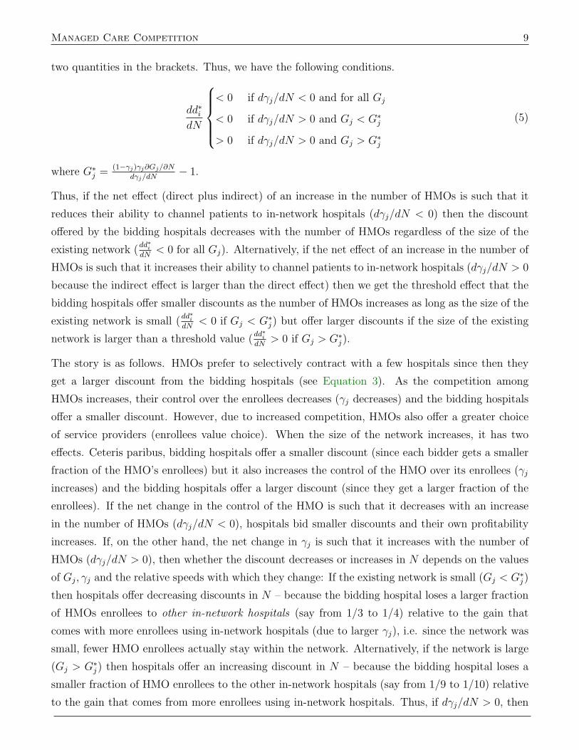
Trends in Procedure and Hospitals with Cath Labs
0
5
10
15
20
25
30
35
40
45
50
1980 1982 1984 1986 1988 1990 1992 1994 1996
Year Total Procedures (in 100,000s) Rate (per 1,000,0000)
Number of Hospitals (in 100s) Percent of Hospitals with CathLabs
Figure 1. Trends in Procedures
Third, starting in the mid 1980s, HMOs experienced a rapid growth. Between 1985 and 1995, the
average number of HMOs per area increased from 4 to 9 and HMO penetration increased from 7%
to 20%. Over the same period, the number of hospitals with cathlabs grew from 18% to about
35%, (see Figure 1) making estimation feasible. Additionally, during this study period, cathlabs
were mainly a hospital technology, i.e., there were no free standing catheterization laboratories and
hence the need to collect additional data (to account for confounding affects due to competition
from single service providers) was eliminated. Several other hospital technologies diffused either
before or after the HMO growth era, or were available outside of the hospital as well.
3.2. Discrete Time Hazard Rate Specification. Following the large body of empirical literature
on technology adoption, I use hazard rate models to estimate the impact of HMOs on the timing of
12Like any other technology, the cost of adopting a cardiac catheterization facility varies with time and geographic location.Typically, the cost can be anywhere between $900K to $1.4M (in 1999) for the basic equipment which includes the X-raymachine. Additionally, if a hospital has to undertake building construction for the laboratory room, the construction costscan be up to $7M more. Construction requirements vary by state. For instance, Pennsylvania requires that the laboratoryfacility have a minimum of 450 square feet area for the laboratory and 150 square feet minimum area for the attached controlroom, with at least 3 inches of building material between the laboratory and the control room, and a window between thetwo rooms. Ohio stipulates that the laboratory area must be at least 600 square feet and the attached control room must beat least 90 square feet. In addition to the X-ray machine and the construction costs, various other pieces of equipment areneeded in the laboratory. These include, a physiological monitor ($90K), pressure injector ($35K), external pace maker ($7K),defibrillator ($9K), emergency cart ($2K), protection material for the laboratory personal ($300 a piece), stainless steel tables($1500), storage cabinets ($3K per unit, need about five of these in a typical laboratory), and finally, film for recording thex-ray images. Initially, 35 mm film were used to capture the results, but the newer facilities have started using cine less filmto capture the images digitally on a computer. The electronic archiving costs can be up to $350K per year.
12 Adoption of Hospital Technology
adoption of cathlabs (Cutler and McClellan, 1996; Baker, 2001; Baker and Phibbs, 2002). Let λi(t)
be the continuous time hazard of adoption in proportional form given by λi(t) = λo(t)exp(xi(t)′β)
where xi(t) are the time varying hospital specific covariates and λo(t) is the baseline hazard function.
Since the data is observed at discrete points, we can generate the discrete time hazard by group
time along the intervals [0, t1), [t1, t2), . . . , [tj,∞). If the covariates are constant during each interval,
then the cumulative adoption probability by the end of period t is given by
Fi(t) = 1− Si(t) = 1− exp{−
t∑j=1
exp(x′ijβ + λj}
(6)
where λj is the natural log of the integrated baseline hazard within an interval (i.e., ln(∫ tjtj−1
λo(τ)dτ})(Meyer, 1990; Prentice and Gloeckler, 1978) and the discrete time hazard, or the probability that
hospital i adopts a cathlab in period [tj−1, tj) conditional on not having already adopted by tj−1 is
given by
λij = Pr[tj−1 ≤ Ti < tj|Ti ≥ tj−1] =Fi(tj)− Fi(tj−1)
1− Fi(tj). (7)
3.3. Hypothesis. How does the conditional probability of adoption λij change with changes in
HMO activity? Combining Equations (6) and (7) and simplifying, we get
λij = 1− exp{−exp(x′ijβ + λj)} (8)
where xij include measures of HMO activity, hospital specific characteristics and other relevant
local area characteristics. Specifically, x2 and x3 are HMO penetration and number of HMOs in the
hospital’s market and x4 and x5 are total number of other hospitals and number of hospitals that
have already adopted the cathlabs by the previous period. Prior literature has often measured HMO
activity at the Health Services Area (HSA) level – an HSA is a cluster of counties – in part because
HMOs compete for enrollees over relatively large geographic areas.13 Following the literature, I also
measure HMO penetration and number of HMOs (x2 and x3) at the HSA level. Whereas HMOs
may compete over relatively large geographic areas, non-speciality hospitals mostly attract patients
from local areas (Gaynor and Vogt, 2003). Thus, rather than measure x4 and x5 at the HSA level,
I computed these variables based on a 24-mile radius using the hospitals’ ZIP codes. Specifically,
for each hospital, x4 counts the number of other hospitals within a 24-mile radius and x5 counts
how many of these neighboring hospitals had already adopted cathlabs by the previous period.
The 24-mile criterion for measuring the characteristics of a local hospital market, while somewhat
arbitrary, has often been used in the medical arms race literature (Luft et al., 1986; Robinson and
Luft, 1987; Robinson et al., 1988) and will be used here as well to facilitate comparison of results
with prior research.
13Briefly, an HSA as a group of counties such that the flow of hospital patients across HSAs is minimized across itsboundaries. For details on grouping algorithm, see Makuc et al. (1991a,b).
Managed Care Competition 13
The conditional probability itself is not linear in the covariates and could increase or decrease with
xk (k = 2, 3) depending on the value of other covariates. For instance, based on the discussion in
section 2, the change in conditional probability of adoption with respect to x3, i.e., ∂λij/∂xij3 could
be positive or negative depending upon how many hospitals have already adopted the technology
i.e., whether x5 is small or large (henceforth the partial is referred to as the marginal probability).
Thus, the specification also includes interaction terms x2x5 and x3x5. Finally, based on the earlier
discussion, I state the following hypotheses:
∂λij∂x2ij
< 0 for all (reasonable) values of x5
∂λij∂x3ij
> 0 if x5 < x∗5 (technology still diffusing)
∂λij∂x3ij
< 0 if x5 > x∗5 (technology already diffused)
(9)
The first hypothesis follows from the findings reported in prior literature that the probability of
adoption decreases with HMO penetration. The second and third follow from my discussion on the
threshold effect in hospital profitability as a function of the number of HMOs (i.e., that dd∗i /dN < 0
if Gj < G∗j and dd∗i /dN > 0 if Gj > G∗j when dγj/dN > 0).
4. Data and Descriptive Statistics
4.1. Data on Cathlabs. The data on the adoption of cathlabs comes from the American Hospital
Association’s (AHA) Annual Survey of Hospitals for the years 1985 through 1995. The AHA survey
annually collects detailed information on hospital characteristics from nearly all U.S. acute care
hospitals and has a response rate of about 90%. Using hospital ID’s, the AHA survey data was
linked across years so that each hospital could be followed from 1985 through 1995 inclusive. The
base line sample was constructed using all non-federal short-term general community hospitals with
non-missing information on cathlabs and on the covariates for each of the these years. In 1985,
there were 5,169 hospitals in the sample of which 775 (15%) had already adopted cathlabs either
during that year or in a prior year. Thus, for the base-line analysis, the sample consisted of
4,394 hospitals that were still ‘at risk’ beginning in 1986. Every year a few new hospitals were
added to the analysis sample. This was not because these were necessarily new hospitals per se,
but rather because in all the previous years there was missing information on covariates on these
hospitals. Thus, for instance, 33 new hospitals were added to the ‘at risk’ population at the end of
1986. Similarly, if a hospital (along with information on its covariates) could not be followed for all
the years until 1995, then it was treated as censored. For instance, 103 hospitals were considered
censored at the end of 1986 because either the hospital ID itself was not present in 1987-1995 AHA
files (merged or closed down) or because information on covariates was missing/miscoded.
14 Adoption of Hospital Technology
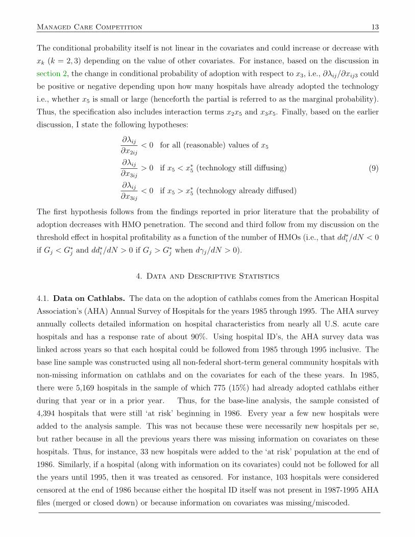
Table 1. Summary of Catheterization Laboratory Adoption Data
Adoptions by Short Term General Community Hospitals between 1986 to 1995‡
Year Hospitals Cathlab Censored New Kaplan-Meier CumulativeAt Risk Adoptions Hospitals† Entries†† Surviver Adoption
(Exits) Function ProbabilitySt 1− St
1986 4394 96 103/8 33/0 0.9782 0.02181987 4220 69 120/9 26/5 0.9622 0.03781988 4053 83 99/5 30/1 0.9425 0.05751989 3897 70 116/7 9/3 0.9255 0.07451990 3716 91 100/4 12/12 0.9029 0.09711991 3545 92 97/14 11/4 0.8794 0.12061992 3357 79 106/4 20/15 0.8587 0.14131993 3203 79 289/5 11/6 0.8376 0.16241994 2847 60 202/0 7/10 0.8199 0.18011995 2602 27 2575/0 0.8114 0.1886
Data Source: American Hospital Association Annual Survey Files
‡ In our sample, 775 hospitals had already adopted cathlabs by 1985. Excluding these, 4,394 hospitals which wereat risk were followed from 1986 onwards. However, an additional 159 hospitals joined the ‘risk set’ starting in alater year making the total sample size of 4,553 unique hospitals that were observed between 1986 and 1995.† Censored hospitals are those that do not adopt in the current year and are (i) either not observed in any of thefollowing years or (ii) reappear in the data set at a later year but not in the following year due to missing covariatevalues. Thus in 1986, 103 hospitals exit permanently while 8 additional hospitals are missing in 1987 but re-enterthe observation set post 1987. Listed exits are counted at the end of the indicated year.†† Entries are either (i) new hospitals with no observations in any of the prior years or (ii) re-entries by hospitals inthe dataset that had a missing covariates in the previous year. Thus in 1994, 7 new hospitals entered the data setwhile 10 re-entered, i.e., had some missing covariates in 1993 but are in the dataset in earlier years. Listed entriesare counted at the end of the indicated year.
Between 1986 and 1995, the total number of non-federal short-term general community hospitals
with cathlabs almost doubled – rising from 775 (15%) at the beginning of 1986 to an additional 746
(about 37%) by the end of 1995 (see Table 1). The fraction of hospitals that adopted each year,
as a percentage of at risk hospitals fluctuated between 1.04% and 2.60% with an average value of
about 2%. The adoption rate was highest in 1991 (2.60% of the at risk population adopted during
that year) and progressively slowed down thereafter.
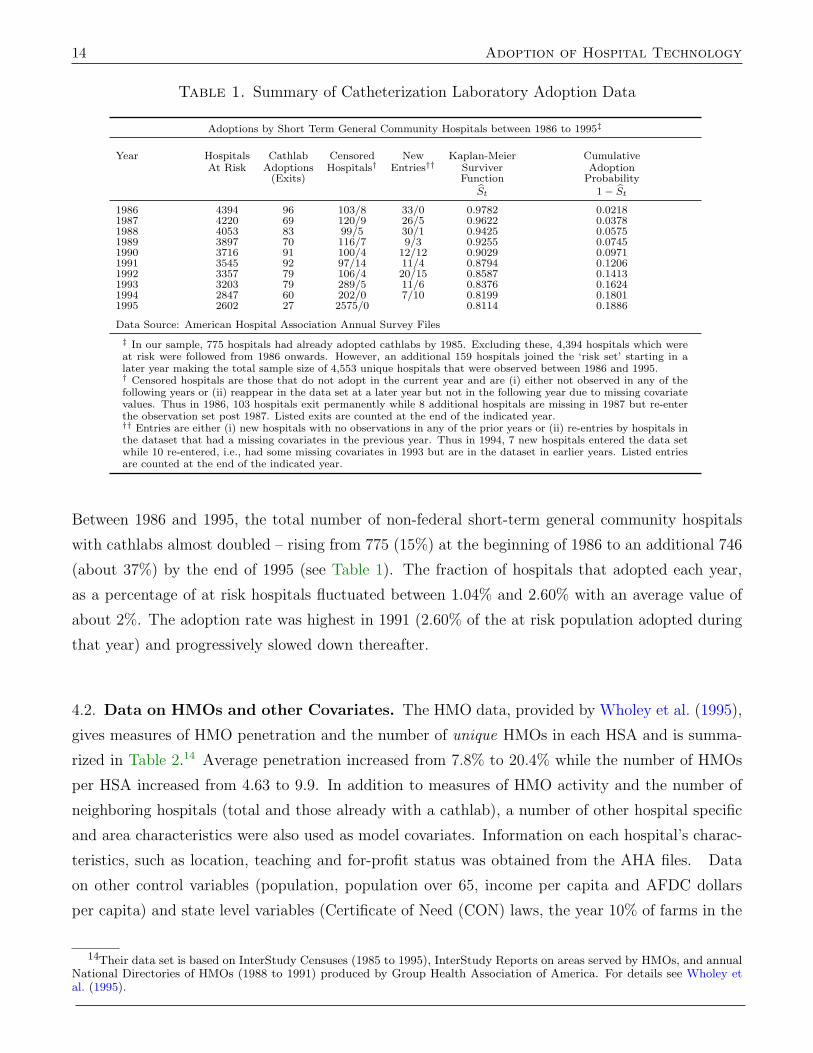
4.2. Data on HMOs and other Covariates. The HMO data, provided by Wholey et al. (1995),
gives measures of HMO penetration and the number of unique HMOs in each HSA and is summa-
rized in Table 2.14 Average penetration increased from 7.8% to 20.4% while the number of HMOs
per HSA increased from 4.63 to 9.9. In addition to measures of HMO activity and the number of
neighboring hospitals (total and those already with a cathlab), a number of other hospital specific
and area characteristics were also used as model covariates. Information on each hospital’s charac-
teristics, such as location, teaching and for-profit status was obtained from the AHA files. Data
on other control variables (population, population over 65, income per capita and AFDC dollars
per capita) and state level variables (Certificate of Need (CON) laws, the year 10% of farms in the
14Their data set is based on InterStudy Censuses (1985 to 1995), InterStudy Reports on areas served by HMOs, and annualNational Directories of HMOs (1988 to 1991) produced by Group Health Association of America. For details see Wholey etal. (1995).
Managed Care Competition 15
Table 2. Descriptive Statistics
Year 1985 1986 1987 1988 1989 1990 1991 1992 1993 1994 1995
Avg. # of HMOs 4.63 6.37 7.28 9.37 9.09 8.92 8.90 9.15 8.85 8.81 9.98Avg. Penetration (%) 7.83 9.73 11.55 13.05 13.68 14.36 14.95 15.88 16.29 17.91 20.37
Note: Data is weighted by HSA population. Thus, the average HSA penetration is also the penetration level for theentire U.S. for the year as well and the average number of HMOs is the average number of unique HMOs per HSA.
Obs = 35,834 Obs = 31,160Mean Std. Err. Mean Std. Err.
x2: HMO penetration 8.902 0.227 9.180 0.214x3: #of HMOs 5.017 0.162 5.028 0.140x4: #of Neighbors 10.854 0.648 8.699 0.394x5: Neighbors w./ cathlabs last year 4.066 0.265 3.290 0.177x2.x5:(HMO Pen)× (Neighbors w./ cathlabs) 79.531 7.432 64.844 4.930x3.x5:(#HMOs)× (Neighbors w./ cathlabs) 57.792 5.781 43.562 3.883x8: 1/0 Dummy - 1 if CON law in state-year 0.733 0.008 0.742 0.007x9: 1/0 Dummy - 1 if located in a rural county 0.086 0.002 . .x10: Year 10% of farms adopted tractors 1929.7 0.151 1930.1 0.141x11: per capita income (1982-84 constant 1000’s $) 12.313 0.056 12.236 0.051x12: per capita AFDC $ (1982-84 constant 1000’s $) 43.445 7.285 33.076 4.617x13: population over 65 (in 100,000s) 0.470 0.049 0.413 0.033x14: square of population over 65 (in 100,000s) 1.892 0.400 1.388 0.252x15: total population(in 100,000s) 4.109 0.495 3.545 0.324x16: 1/0 Dummy - 1 if for-profit 0.125 0.005 0.126 0.004x17: 1/0 Dummy - 1 if medical school affiliated 0.060 0.002 0.057 0.002
Note 1: Standard Error of the mean is clustered where clusters are over HSAs and years.Note 2: The statistics are from two samples.Obs = 35,834: Pooled hospital-year observations (1986-1995) for hospitals ‘at risk’ beginning of 1986.Obs = 31,160: Same as above, except observations on new hospitals, those in rural areas, and those from very dense areashave been removed.
state adopted tractors) were obtained from Area Resource File (1996 CD) and published reports
on state laws. The data on these covariates is summarized in Table 2.15
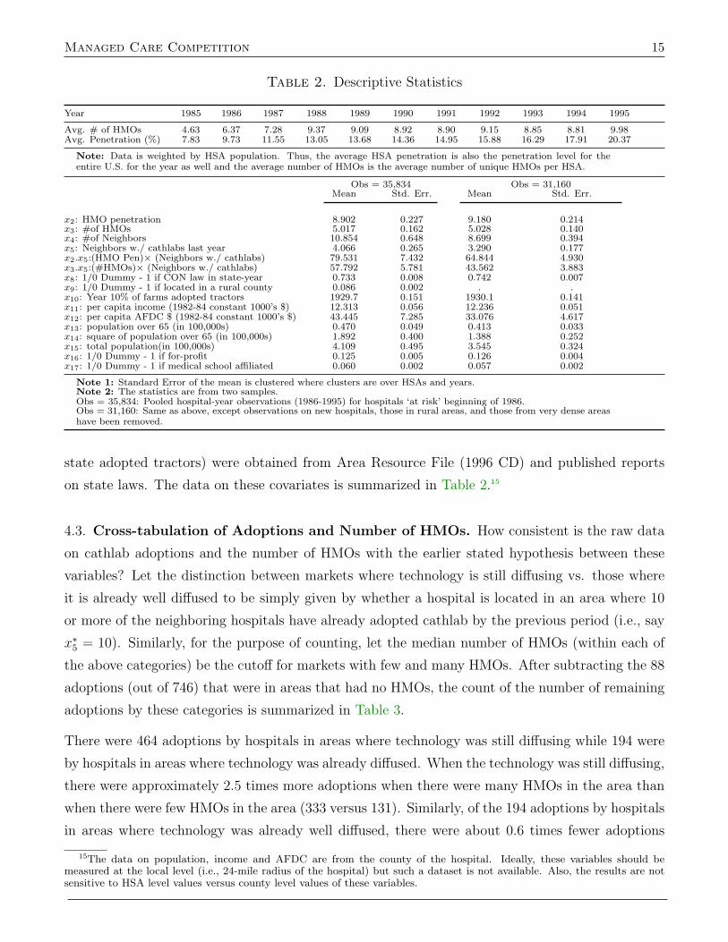
4.3. Cross-tabulation of Adoptions and Number of HMOs. How consistent is the raw data
on cathlab adoptions and the number of HMOs with the earlier stated hypothesis between these
variables? Let the distinction between markets where technology is still diffusing vs. those where
it is already well diffused to be simply given by whether a hospital is located in an area where 10
or more of the neighboring hospitals have already adopted cathlab by the previous period (i.e., say
x∗5 = 10). Similarly, for the purpose of counting, let the median number of HMOs (within each of
the above categories) be the cutoff for markets with few and many HMOs. After subtracting the 88
adoptions (out of 746) that were in areas that had no HMOs, the count of the number of remaining
adoptions by these categories is summarized in Table 3.
There were 464 adoptions by hospitals in areas where technology was still diffusing while 194 were
by hospitals in areas where technology was already diffused. When the technology was still diffusing,
there were approximately 2.5 times more adoptions when there were many HMOs in the area than
when there were few HMOs in the area (333 versus 131). Similarly, of the 194 adoptions by hospitals
in areas where technology was already well diffused, there were about 0.6 times fewer adoptions
15The data on population, income and AFDC are from the county of the hospital. Ideally, these variables should bemeasured at the local level (i.e., 24-mile radius of the hospital) but such a dataset is not available. Also, the results are notsensitive to HSA level values versus county level values of these variables.
16 Adoption of Hospital Technology
Table 3. Number of cathlab adoptions broken by – number of HMOs in the areavs. number of neighbors already with cathlabs.
Technology still diffusing: Technology well diffused:(Neighbors w. cathlabs < 10) (Neighbors w. cathlabs ≥ 10)
# of HMOs ≤ median † 131 126# HMOs > median † 333 68
† The median value for number of HMOs was 2 for hospitals that were in areas whereless than 10 neighbors had already adopted the cathlabs. Similarly, the median value fornumber of HMOs was 14 for hospitals that had 10 or more neighbors with cathlabs.
when there were many HMOs in the area than when there were fewer HMOs in the area (68 versus
126). Thus, the counts of number of adoptions as summarized in Table 3 is consistent with the
hypotheses about the effect of the number of HMOs on adoption probabilities. This cross-tabulation
is merely suggestive and I test the hypothesis more formally in the next section.
5. Estimates from Hazard Rate Models
There is a significant amount of variation in hospital and area characteristics of these hospitals.
For instance, in the full sample (obs = 35,834), while the mean value of HMO penetration is 8.9%
(s.e. = .227), the actual values range from 0 to 70% in the HSA of the hospital. Similarly, for
each hospital there are on average about 11 neighboring hospitals (s.e. = .162) within a 24 miles
radius, the actual number ranges from 0 (in rural areas) to about 134 hospitals (in some very dense
areas such as those in Los Angeles, New Jersey, New York etc.). While some of the differences in
the size of the market (which may influence the adoption decision) can be controlled for via either
population variables or dummy variables to indicate that the hospital is located in a rural county,
it is possible that the hospitals in rural or very dense areas behave differently than those in the rest
of the country. In order to account for such a possibility, I estimated the hazard function under
numerous specifications and under slightly modified versions of the data, i.e., either by dropping
observations from rural areas, or from very dense areas, or both. The main results are summarized
in Table 4 and are labeled ’1’ through ’7’. Column 1 provides estimates when all observations
(n = 35, 834) were used, including hospitals in rural areas as well as those in very dense markets.
The coefficient on the number of neighbors (x4) is negative but the coefficient on the number of
neighbors with cathlabs (x5) is positive indicating that it is not the number of neighbors but rather
the number of neighbors that offer the same technology in the previous period that increases the
likelihood of a hospital to adopt the technology. Similar results were observed by Luft et al. (1986)
when analyzing adoption data on cardiac catheterization. To investigate this aspect further, the
model was re-estimated by excluding the variable on the number of neighbors with catheterization
laboratories in the previous period from the specification (results not shown). The coefficient on the
number of neighbors then became positive and significant. The two results combined indicate that

Managed Care Competition 17
Table 4. Discrete Time Hazard Rate Estimation
Specifications(1) (2) (3) (4) (5) (6) (7)
Variable Selected Coefficients and Standard Errors(1)
x2: HMO Penetration -.0139b -.0145b -.0145b -.0119 -.0119 -.0104 -.0039(.0071) (.0074) (.0074) (.0074) (.0074) (.0074) (.0075)
x3: #of HMOs .0456a .0466a .0465a .0428a .0427a .0406a .0377a
(.0126) (.0130) (.0130) (.0134) (.0134) (.0132) (.0137)
x4: #of Neighbors -.0316a -.0334a -.0335a -.0280a -.0282a -.0287a -.0296a
(.0065) (.0067) (.0067) (.0072) (.0072) (.0072) (.0072)
x5: Neighbors w./ Cath- .1126a .1200a .1202a .1323a .1324a .1301a .1221a
labs last year (.0194) (.0201) (.0201) (.0200) (.0200) (.0201) (.0202)
x2.x5:(HMO Pen)× .0006 .0007 .0007 -.0000 -.0000 .0001 -.0002(Neighbors w./ Cathlabs) (.0005) (.0005) (.0005) (.0005) (.0005) (.0005) (.0005)
x3.x5:(#HMOs)× -.0047a -.0050a -.0050a -.0050a -.0050a -.0050a -.0040a
(Neighbors w./ Cathlabs) (.0008) (.0008) (.0008) (.0009) (.0009) (.0009) (.0009)
x8: CON Law Dummy. 1 if .2322b .1010law in effect in state-year (.1083) (.1103)
x9: Year 10% of Farms .0296a
adopted tractors (.0057)
x10: Rural area dummy. -3.1564a -3.1238a -3.1053a
1 if rural area (.7095) (.7096) (.7098)
Marginal with respect to: Selected Marginals (∂λij
∂xk) and Standard Errors
x2: HMO Penetration -.00018b -.00018b -.00023b -.00018b -.00024b -.00021c -.00009(.00010) (.00010) (.00013) (.00010) (.00013) (.00013) (.00013)
x3: #of HMOs .00041b .00041b .00050b .00042a .00054a .00049b .00048b
(.00018) (.00018) (.00024) (.00018) (.00024) (.00024) (.00024)
exclude new hospital obs? (2) x X X X X X Xexclude rural area obs? (3) x x X x X X Xexclude dense area obs? (4) x x x X X X X
# of Hospitals @ risk end of ’85 4394 4394 4060 4267 3933 3933 3933# of Observations used 35834 35103 32033 34230 31160 31160 31160# of Events 746 716 714 708 706 706 706Log Likelihood -3374.87 -3246.24 -3228.47 -3195.91 -3178.18 -3175.62 -3160.29
Significance of estimates at 1%, 5% and 10% level indicated by a b c respectively. Clustered s.e. are in parenthesis.
Note 1 (Other Variables – See Appendix B): All specifications include 10 time dummies (i.e., baseline hazardparameters) & variables for per capita income, AFDC per capita, total population, population 65+ and sq. of pop65+ in the hospital market. Additionally, the regressions also include dummy variables to indicate a hospital’sfor-profit and teaching school status. Coefficients on these additional variables had expected signs and are given inAppendix B.Note 2 (New Hospital Observations): A total of 159 hospitals that entered the observation set post 1986 weredropped from the analysis. See table 2.Note 3 (Rural Areas Observations): A county is considered rural if it is not adjacent to a metro area and ifno city within the county has population greater than 2,500. For these counties, the total population varies from1,300 to about 36,000.Note 4 (Dense Areas Observations): These included hospitals in the following 7 MSAs/PMSAs: Bergen-Passaic, Newark & Jersey City in NJ Los Angeles-Long Beach & Orange Cnty in CA and Nassau-Suffolk & NewYork City in NY
the overall results are consistent with the medical arms race literature. The coefficient on HMO
penetration (x2) is negative and statistically significant and is consistent with results reported in
Baker (2001) and Baker and Phibbs (2002). However, the coefficient on the number of HMOs (x3)
is positive and significant indicating that as the number of HMOs increases, the adoption hazard
increases.
18 Adoption of Hospital Technology
The specification also includes interaction terms between x5 and the HMO variables. The interaction
term with HMO penetration (x2.x5) is not statistically significant but the interaction term with the
number of HMOs is negative and statistically significant (x3.x5). Further, this interaction term is
about one order of magnitude smaller than the coefficient on the number of HMOs. In the lower part
of Table 4, I provide estimates of the marginal probabilities (∂λij/∂xk for xk = x2 and x3) computed
at the sample mean.16 Thus, in specification 1, at the sample mean, an incremental increase in HMO
penetration decreases the probability of adoption (conditional on not having already adopted) by
-.00018 while an incremental increase in the number of HMOs increases the adoption probability
(conditional on not having already adopted) by +.00041 and the results are statistically significant.
5.1. Unobserved Heterogeneity.
5.1.1. New Hospitals. Table 1 shows that 159 new hospitals entered the observation set after
1986. These ‘new’ hospitals were either truly new hospitals, old hospitals with no observations in
the AHA files for the previous years, or possibly the result of mergers. It is possible that these new
hospitals could be (partially) driving the results because they have a different baseline hazard and
are in areas where there are more HMOs. To account for this possibility, I omitted all observations
on these 159 hospitals and re-estimated the model. The results, given in column 2 of Table 4, are
essentially the same as those in column 1 (which include observations on these 159 hospitals). In
all remaining specifications, I exclude these 159 hospitals from the analysis.
Table 1 also shows that there were several hospitals that exited the observation set prior to 1995.
For instance, 100 hospitals could not be followed 1990 onwards in the AHA dataset and had not
adopted the cathlabs by 1989. In the usual language of time to event models, they are considered
censored observations and only contribute to the likelihood function until they are censored. As such
no special treatment for these hospitals is needed as long as the censoring mechanism itself is non-
informative. But if the censoring itself is primarily due to merger/closing, which itself is correlated
with probability of adoption, then the usual concerns about sample selection apply. An example
would be if the censored observations are from hospitals for whom a large number of neighbors have
already adopted the cathlabs, and the non-adopters exit the market since they cannot get favorable
contracts from HMOs. To check this, I re-estimated the model by also excluding an additional 1,232
hospitals (= 103 + 120 + . . .+ 202) from the risk-set. The results were virtually the same as those
16Marginals were computed at the sample mean (i.e. at Xi = X) as follows: Let Λ be the transformation such that
Λ(I) = 1 − exp(−exp(I)) where I = Xβ and X is the full data matrix then∂λij
∂xk= ∂Λ
∂I. ∂I∂xk
where ∂Λ∂I
= exp(I − exp(I)).
The significance is established by the delta method. For instance, for the marginal wrt number of HMOs (xk = x3) the
computation is as follows: Let h(β) =∂λij
∂x3. Then h(β) =
∂λij
∂x3= F ′(I)∂I/∂x3 = exp
(− exp(I)
)exp(I)
(∂I/∂x3
)where
I = βT X and the s.e. is the square root of the leading diagonal of ∇ThVc∇h where ∇h is a k×1 vector with the jth row given
by F ′′(·) ∂I∂x3
∂I∂βj
+ F ′(·) ∂2I∂βj∂x3
and where F ′′(·) = F ′(·)(
1 − exp(I))
and Vc is the estimated (clustered) variance-covariance
matrix of β.
Managed Care Competition 19
reported in column 2 (not shown) and hence in the rest of the specifications, I do not exclude these
additional 1,232 hospitals (so as not to reduce the sample size too much).
5.1.2. Hospitals in Rural/Dense Areas. Since it is possible that the hospitals in rural or very
dense areas behave differently from those in the rest of the country, I re-estimated the hazard rate
model by omitting observations from these areas. Column 3 does not include hospitals in rural
counties, column 4 drops observations from areas where hospital markets are dense, specifically
if a hospital has more than 100 neighbors, and column 5 drops both type of observations. In all
three specifications, the results are virtually the same as those in earlier specifications. The main
difference is that by dropping observations from the rural areas the point estimates of the marginal
probabilities change by a small amount. For instance, by excluding observations from the rural
areas, the marginal probability with respect to HMO penetration changes from -.00018 to about
-.00024 and the marginal with respect to number of HMOs changes from about .00041 to .00054.
These results were robust to alternative definitions of rural counties as well as to alternative cut-offs
of 80 and 120 neighbors definition for dense markets. Henceforth, I drop all observations from rural
areas and dense areas (and observations on new hospitals).
5.1.3. State Level Differences. States differ in regulating the acquisition of new hospital tech-
nologies. Hospitals in states with stricter laws would be less likely to adopt new expensive tech-
nologies. Certificate of Need (CON) laws are one such instrument used by states to control the
diffusion of technology (and cost more generally). Since prior research has shown the ineffectiveness
of CON laws to reduce the diffusion of technology (or costs) (Salkever and Bice, 1976; Sloan and
Steinwald, 1980; Joskow, 1981), it is the primary reason why I have omitted such variables from
the present model. (In fact, in a similar hazard rate model, Cutler and McClellan (1996) found the
coefficient on the dummy variable for CON laws to be not statistically significant). However, in
column 6, I include a simple dummy variable (x8) to capture if the Certificate of Need (CON) laws
were present in the state-year of the hospital.17 The coefficient on the CON law dummy is positive
and significant. This may be due to the fact that states where technologies spread more rapidly
were the ones that were more likely adopted these CON laws. However, the coefficients on HMO
variables have the same sign and significance as the earlier specifications.
In addition to differences in the regulatory environment across states, there may be a number of other
intangible variables that may affect the cathlab adoption hazards of hospitals. For instance, Skinner
and Staiger (2005) show that some states are consistently early adopters of many technologies
(hybrid corn, tractors, Beta Blockers etc.) and that these early adopting states also had higher
17A simple dummy variable does not capture the intra-state differences in the strictness of these laws (e.g. capital limits)but richer data was not available.
20 Adoption of Hospital Technology
values of the (Putnum) Social Capital index.18 Thus, it may be the case that whatever drives early
adoption of various technologies in these states (whether it be social capital or something else) could
also influence the adoption probabilities of cathlabs. If any of these variables are correlated with the
included variables in the model, for instance if HMOs selectively enter markets with greater social
capital, then leaving them out would cause an omitted variable bias.19 To this end, I re-estimated
the model with all variables given in specification 6 but also added a number of variables that
capture such intangible differences across states (one variable at a time) to assess if the coefficients
on HMO related variables change in any significant way. The results from adding one such variable,
the year 10% of farms in the state adopted tractors, are given in column 7. The other variables
that I included in the specification (in lieu of the year 10% farms achieved tractors) include, (1)
year 10% of farms adopted hybrid corn, (2) percent of farms that adopted tractors in year Y (where
Y was 1920, 1930, 1940, 1949, or 1959 respectively), (3) % in homes with computers in 1993, (4)
Putnum Social Capital Index and, (5) Putnam Education Index.20 All of these variables are highly
correlated with each other and gave the same results as those shown in column 7, specifically, that
the coefficient on the HMO penetration variable was not significant but that the coefficient on the
number of HMOs stayed positive and significant.
5.2. Robustness. In all the seven specifications, the marginal probability with respect to the
number of HMOs at the sample mean is positive, i.e., at the sample mean a small increase in the
number of HMOs increases the (conditional) probability of adoption (by +.00040 in specification
1 and by +.00048 in specification 7). Similarly, in all specifications the marginal probability with
respect to HMO penetration is negative (and in all but the last case is statistically significant – in
the last specification, the p-value for the marginal was .21 – the highest ever observed across all
specifications including those that are not shown in Table 4).
In addition to the variation in specifications above, I also estimated the hazard rate using (1) logit
specification (instead of the complementary log-log), (2) measuring HMO variables at the county
level (instead of HSAs), and (3) alternative measures of HMO competition, specifically either the
18The term “Social Capital” has widely different meanings across different circles. As used by Robert Putnam (1995; 2000)it refers to externalities due to informational and social networks. The Social Capital Index itself consists of an aggregatedvalue of 14 sub-indexes ranging from questions about life styles of the individuals (“number of club meetings attended in lastyear”) to counts of non-profit organizations in the area/state. See also http://www.bowlingalone.com/data.php3.
19The most straight forward way of dealing with such time-invariant omitted variables is to include state level dummiesin the set of control variables. However, such a strategy was not feasible in the current estimation: Including 50 state-leveldummy variables on top of the 10 time dummies already included in all specifications (and after dropping observations on newhospitals, rural areas and very dense areas) leaves a total of 706 ‘events’ to be distributed over 50 × 10 cells. Also note thatestimation procedure involves excluding all hospitals from the observation set that had already adopted before 1986 as wellas removing all observations on a hospital after it has adopted the technology since the remaining years observations do notmake any contribution to the likelihood function. Such a strategy was attempted, but predictably, it lead to non-significanceon all the included variables.
20Following Griliches (1957), the year 10% of farms in the state adopted tractors was computed by Skinner and Staiger(2005). I am in debt to Doug Staiger for providing data on all of the above mentioned variables, including data on the Putnumindicators.
Managed Care Competition 21
Herfindahl index, its inverse, or number of HMOs per capita (instead of number of HMOs). In all
cases the results were qualitatively similar (and are available from the author upon request).
5.3. Endogeneity. It is possible that some unobserved local market factors that may be changing
over time affect both, hospitals’ decision to adopt the technology of interest, and the HMOs’ decision
to enter the market (and hence HMO penetration level and the level of competition among HMOs).
For instance, Baker (1996) and Baker and Spetz (1999) argue that markets with more aggressive
practices may be more attractive to HMO entry as well as more likely to adopt technology. If true,
failure to include a variable that is correlated with both may lead to the usual omitted variables
bias. If the ‘aggressiveness’ of a market is adequately captured by the variable x5 (neighbors that
have already adopted cathlab by the previous period) then concerns about possible endogeneity
due to correlation of the HMO variables with the error term may be alleviated to some extent.
Nonetheless, in this section I treat the HMO variables (x2, x3 and their interactions with x5) as
potentially endogenous. Additionally, it is possible that x5 by itself is also endogenous. Note that
x5 does not cause a simultaneity bias per se, since it is equal to the number of hospitals that had
adopted catlabs by the previous period, i.e., is a lagged variable in the specifications. However, it
may still lead to biased estimates due to other reasons – specifically a hospital may adopt technology
to discourage or encourage future adoptions by other hospitals – in which case it would be correlated
with the censoring mechanism. I already considered this possibility earlier by comparing hazard
rate results from the full sample with those where I excluded 1,232 hospitals that closed prior to
adopting cathlabs (see discussion in Section 5.1.1 on page 19). Since the estimates did not change,
it is unlikely that x5 is endogenous. However, in this section, I use the instrumental variables
approach and account for possible endogeneity of this variable as well.
Due to the qualitative nature of some of the right hand side variables of interest (number of HMOs,
number of neighbors with cathlabs etc.), I first re-estimate the hazard model as a linear probability
model and compare it with the results in Table 4. Next, I use the GMM-IV methods on the linear
probability model (treating the number of HMOs and neighbors with cathlabs as quantitative
variables) and test how much the estimated coefficients change if the HMO variables (and x5) are
endogenous. While not conclusive, however, if in the linear probability models endogeneity is not a
serious issue (say on the basis of the Hausman test), then it is indicative that the results in Table 4
are not seriously biased on account of endogeneity of these variables.21
21The complementary log-log model in Equation 8 was generated by grouping time in the continuous-time proportionalhazard model into intervals (for details see Meyer (1990)). Alternatively, the probability to adopt (conditional on not havingalready adopted) can be written as λij = F (x′ijβ+λj) where F (·) is the cumulative distribution function of the latent variable.If the latent variable has a standard extreme value distribution, then once again we get the complementary log-log hazardrate model. However, if F (·) is an identity function then we get a linear probability model λij = x′ijβ + λj + υij where x2, x3
and the interactions with x5 are allowed to be correlated with the error term (as well as x5 itself).
22 Adoption of Hospital Technology
5.3.1. Instruments. Large employers are more likely than small employers to offer their employees
a choice of insurance plans, including the choice to enroll in HMOs. This is partly because a
federal law mandates that firms with more than 25 employees must offer their employees the choice
to join an HMO, providing that the firm offers an insurance plan and there is an HMO in the
market that wishes to be included. This suggests that markets with large employers will be more
attractive to HMO entry making it a relevant instrument. Dranove et al. (2003) used a variation
of the later variable in a model that predicts the number of HMOs in an area and found it to be
significant. Additionally, it would also be a valid instrument as long as large employers do not
directly influence provider behavior independently of the effect of HMOs. In a related study on
number of mammography providers in an area, Baker and Brown (1997, 1999) report that the
number of large businesses as an instrument for HMO variables satisfied the exclusion restrictions.
Thus, my first instrument is the number of firms with 100 or more employees per capita in the HSA
(henceforth z1).
Independent of the effect of large employers on HMOs, several state regulations may also alter the
incentives for HMOs to enter in local markets or their ability to expand in these markets. For
instance, the enactment of “any willing provider” and “freedom of choice” laws (henceforth AWP
or FOC), which are often lobbied by providers (hospitals, physicians and pharmacies) may be seen
as preemptive strikes to prevent or delay the emergence of selective contracting in their markets.
The AWP laws require HMOs to accept any provider in their network who is willing to abide by the
rules of a standard contract with other providers. This implies that an HMO would have a limited
ability to extract large discounts from providers in exchange for a large/concentrated volume which
in turn would restrict HMO growth in these markets. One study (Sheils et al., 1995) estimates
that the AWP laws resulted in 6.9% slower increase in HMO enrollment over the period 1985-1994.
The FOC laws would have a similar impact on HMOs, however, the mechanism is different. The
FOC laws require HMOs to allow patients to go outside the network to obtain covered services from
non-network providers. The main difference is that the managed care firm may pay the provider
a price typically below the price negotiated with network providers, but the patient is required
to make a larger copayment. Additionally, the FOC law sometimes allows the new provider to
balance-bill the patient. The FOC law primarily effects the HMO growth via price elasticity of the
out-of-pocket payments. Thus, AWP and FOC laws restrict HMOs in different ways and the latter
may be viewed as a ‘consolation prize’ for proponents (hospitals, physicians, pharmacies) who do
not have a strong enough lobby to help enact AWP laws (see Ohsfeldt et al. (1998)). I use FOC
and AWP laws as second and third instruments respectively (z2 and z3).22 Additionally, large firms
22There are separate AWP and FOC laws for HMOs and other forms of managed care (e.g. PPOs). Further, they specify ifthe FOC or AWP law applies to hospitals, physicians or pharmacies. In my construction of these instruments, I only considerif the FOC or AWP law applies to HMOs (rather than to PPOs). Thus, variable z2 for FOC and z3 for AWP took four possiblevalues (0,1,2,3) and each variable was constructed by summing three dummy variables indicating if the state had a FOC orAWP law for HMOs regarding (i) physicians, (ii) hospitals, or (iii) pharmacies in a given year.
Managed Care Competition 23
which can choose to self-insure are sometimes exempt from FOC/AWP laws. Thus, two markets
with the same AWP/FOC laws may not be equally attractive to HMOs if one has more large firms
than the other. Hence, in some estimates, I also used an interaction of these three instruments as
an additional instrument (i.e., z4 = z1z2z3).
To construct an independent instrument for x5 (neighbors with cathlabs in the previous period)
I rely on an assumption already used in the main hazard rate model: That a hospital’s decision
to adopt depends on the neighbors’ characteristics (for instance how many of its neighbors have
already adopted) but not on hospitals that are not its neighbors. Thus, for each hospital, I first
identified neighbors’ neighbors, and then excluded from this set all hospitals that were also the
original hospital’s neighbors. Characteristics of these non-overlapping neighbors’ neighbors would
partially influence the adoption decisions by neighbors’ (a relevant instrument), but not the original
hospital’s decision (a valid instrument) except via their influence on the intermediary neighbors.
Thus, I constructed the additional instrument z5 as the number of neighbors’ neighbors who are
not the original hospital’s neighbors and had also already adopted cathlabs. Finally, note that the
main specification includes interaction terms between the HMO variables and the neighbors with
cathlabs variable. Thus, in the ‘first-stage’ I also use the interactions between the instruments for
these variables as additional instruments (see Wooldridge (2002) pp. 231-235).
My primary interest here is to check if the coefficients change by a significant amount when the
HMO variables and their interaction with x5 are allowed to be endogenous. To this end I com-
pute Hausman’s statistic (χ2 = (β2 − β1)T (V2 − V1)−1(β2 − β1)) using the GMM estimators for
heteroscedastic OLS (H-OLS) and heteroscedastic 2SLS (H-2SLS).23 Results are summarized in Ta-
ble 5. The first column redisplays the results from specification (4) of the discrete time hazard model
and the second column (labeled H-OLS(4A)) provides H-OLS estimates of the linear probability
model (LPM) for specification (4). Note that for H-OLS, x2, x3, x5 and the interaction terms are
treated as exogenous. The difference in the magnitude of the coefficients in column 1 and column
2 is somewhat misleading since, in the linear model, but for the interaction term, the coefficients
are the marginals, whereas for the probability model in column 1, the marginals are given by the
partial of a cloglog function (see footnote 16). Accounting for the interaction term, the marginals
with respect to x2 and x3 are comparable in magnitude and are given in the middle section of the
table. For instance, the marginal with respect to number of HMOs in specification (4) is .00042 but
for the linear model with H-OLS estimates, it is .00053.
23H-OLS, due to Cragg (1983), is a two-step GMM estimator that uses the additional moment conditions when thereare excluded exogenous instruments and it is asymptotically more efficient than the usual ‘robust’ OLS estimator underheteroscedasticity. Similarly, the H-2SLS, due to Davidson and Mackinnon (2004, see p.365), is also a GMM estimator and ismore efficient than the robust 2SLS estimator.
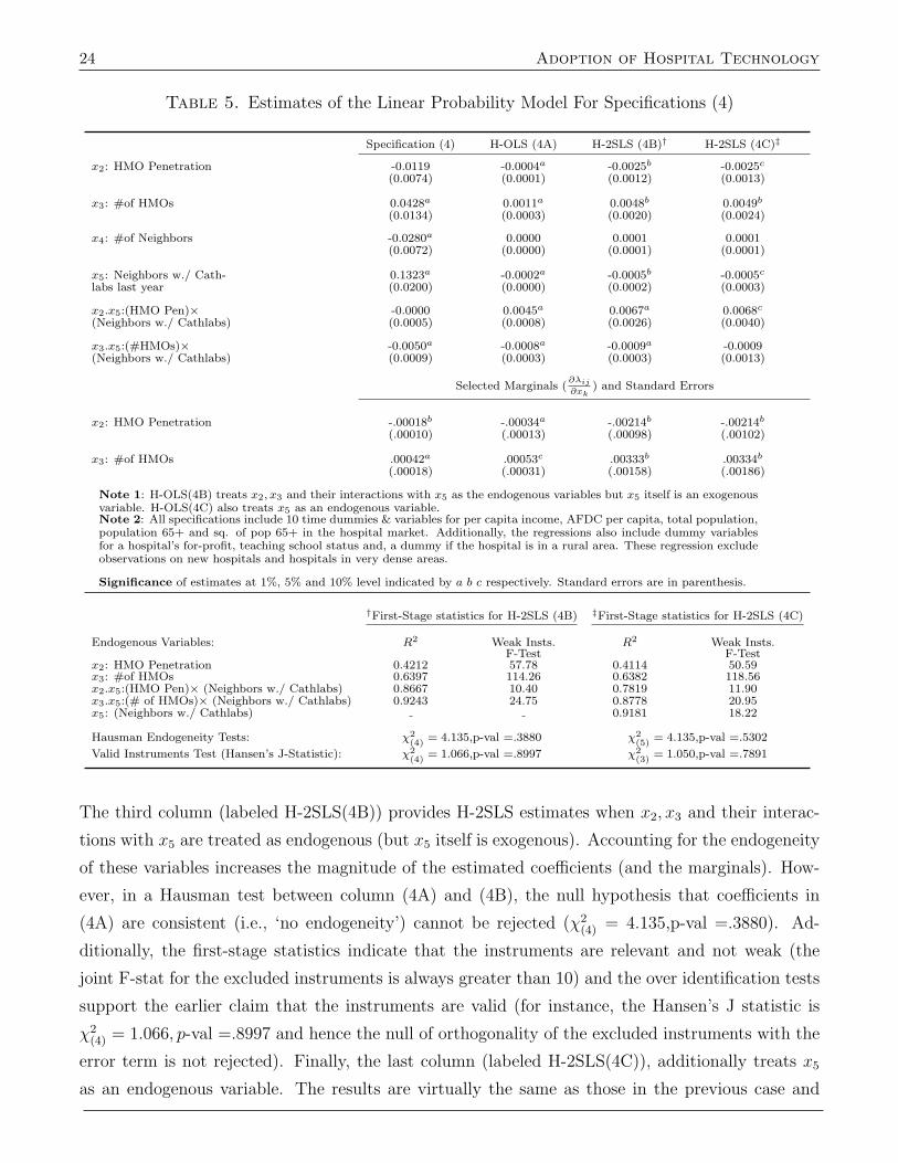
24 Adoption of Hospital Technology
Table 5. Estimates of the Linear Probability Model For Specifications (4)
Specification (4) H-OLS (4A) H-2SLS (4B)† H-2SLS (4C)‡
x2: HMO Penetration -0.0119 -0.0004a -0.0025b -0.0025c
(0.0074) (0.0001) (0.0012) (0.0013)
x3: #of HMOs 0.0428a 0.0011a 0.0048b 0.0049b
(0.0134) (0.0003) (0.0020) (0.0024)
x4: #of Neighbors -0.0280a 0.0000 0.0001 0.0001(0.0072) (0.0000) (0.0001) (0.0001)
x5: Neighbors w./ Cath- 0.1323a -0.0002a -0.0005b -0.0005c
labs last year (0.0200) (0.0000) (0.0002) (0.0003)
x2.x5:(HMO Pen)× -0.0000 0.0045a 0.0067a 0.0068c
(Neighbors w./ Cathlabs) (0.0005) (0.0008) (0.0026) (0.0040)
x3.x5:(#HMOs)× -0.0050a -0.0008a -0.0009a -0.0009(Neighbors w./ Cathlabs) (0.0009) (0.0003) (0.0003) (0.0013)
Selected Marginals (∂λij
∂xk) and Standard Errors
x2: HMO Penetration -.00018b -.00034a -.00214b -.00214b
(.00010) (.00013) (.00098) (.00102)
x3: #of HMOs .00042a .00053c .00333b .00334b
(.00018) (.00031) (.00158) (.00186)
Note 1: H-OLS(4B) treats x2, x3 and their interactions with x5 as the endogenous variables but x5 itself is an exogenousvariable. H-OLS(4C) also treats x5 as an endogenous variable.Note 2: All specifications include 10 time dummies & variables for per capita income, AFDC per capita, total population,population 65+ and sq. of pop 65+ in the hospital market. Additionally, the regressions also include dummy variablesfor a hospital’s for-profit, teaching school status and, a dummy if the hospital is in a rural area. These regression excludeobservations on new hospitals and hospitals in very dense areas.
Significance of estimates at 1%, 5% and 10% level indicated by a b c respectively. Standard errors are in parenthesis.
†First-Stage statistics for H-2SLS (4B) ‡First-Stage statistics for H-2SLS (4C)
Endogenous Variables: R2 Weak Insts. R2 Weak Insts.F-Test F-Test
x2: HMO Penetration 0.4212 57.78 0.4114 50.59x3: #of HMOs 0.6397 114.26 0.6382 118.56x2.x5:(HMO Pen)× (Neighbors w./ Cathlabs) 0.8667 10.40 0.7819 11.90x3.x5:(# of HMOs)× (Neighbors w./ Cathlabs) 0.9243 24.75 0.8778 20.95x5: (Neighbors w./ Cathlabs) 0.9181 18.22
Hausman Endogeneity Tests: χ2(4)
= 4.135,p-val =.3880 χ2(5)
= 4.135,p-val =.5302
Valid Instruments Test (Hansen’s J-Statistic): χ2(4)
= 1.066,p-val =.8997 χ2(3)
= 1.050,p-val =.7891
The third column (labeled H-2SLS(4B)) provides H-2SLS estimates when x2, x3 and their interac-
tions with x5 are treated as endogenous (but x5 itself is exogenous). Accounting for the endogeneity
of these variables increases the magnitude of the estimated coefficients (and the marginals). How-
ever, in a Hausman test between column (4A) and (4B), the null hypothesis that coefficients in
(4A) are consistent (i.e., ‘no endogeneity’) cannot be rejected (χ2(4) = 4.135,p-val =.3880). Ad-
ditionally, the first-stage statistics indicate that the instruments are relevant and not weak (the
joint F-stat for the excluded instruments is always greater than 10) and the over identification tests
support the earlier claim that the instruments are valid (for instance, the Hansen’s J statistic is
χ2(4) = 1.066, p-val =.8997 and hence the null of orthogonality of the excluded instruments with the
error term is not rejected). Finally, the last column (labeled H-2SLS(4C)), additionally treats x5
as an endogenous variable. The results are virtually the same as those in the previous case and

Managed Care Competition 25
all test statistics lead to the same conclusions (also reported at the bottom of the table). These
results show that the potential endogeneity of HMO variables (or of the number of neighbors) does
not pose any serious problem in the estimation of the linear probability model when endogeneity
is ignored. In turn this suggests that, even if HMO variables are endogenous, the coefficients and
marginals reported in Table 4 may not be necessarily biased.24
6. Marginal Effects and Net Adoptions
In all the seven specifications summarized in Table 4, the coefficient on HMO penetration is negative
while that on the number of HMOs is positive. However, given the non-linear nature of the hazard
(see Equation 8) as well as the interaction terms, it is not immediately clear if the hazard (λij)
increases or decreases with x2 and x3 over the range of the data. For instance, since the coefficient
on the interaction term (x3.x5) between neighbors with catheterization laboratories (in the last
period) and the number of HMOs is negative and smaller by about an order of magnitude than the
coefficient on the number of HMOs (x3), the slope of the probability curve will become negative
when the number of neighbors with a catheterization laboratory is some value slightly greater than
ten.
6.1. λij vs. x3 (given x5). To show this, Figure 2 plots the discrete hazard, i.e., the conditional
probability of adoption given that the hospital has not already adopted (see Equation 8) as a function
of the number of HMOs where all other variables are at the sample mean but the number of hospitals
that had already adopted in the previous period is fixed at 0,3,6,10,12, and 15 respectively. The first
panel of Figure 2 plots all the graphs together and the remaining panels display the same probability
graphs along with the 95% confidence intervals. Two things are worth noting from these graphs.
First, at all levels of x5 when the number of HMOs increases from zero to one, there is a dip in the
curves showing that the probability of adoption decreases. This is a pure penetration effect since
there is only one HMO in the market. However, this result is not statistically robust, as evidenced
from large error bars shown in the other five panels of this figure, especially for high values of x5
(at low values of number of HMOs). The error bars are large since the simulations at this point are
mostly out of sample. For instance, there are no observed markets where 12 neighboring hospitals
have already adopted cathlabs and there are no HMOs in the market.25 Second, when the number
of neighbors that had already adopted is low (x5 = 0, 3 or 6), the probability curve (as a function
24The results were also robust to several alternative versions of the excluded instruments. For instance, in (4B) since it isassumed that x5 is exogenous, it is possible to construct alternative instruments as the interaction of x5 with the instrumentsfor the HMO variables. The results from these alternative instruments are available from the author upon request.
25In other versions, I tried to isolate this pure penetration effect by including a dummy variable for exactly one HMO inthe market but the results were not significant and of the ‘wrong’ sign since the comparison group would be both sides: zeroHMOs and two or more HMOs. I also tried using spline methods and/or selecting sub-samples for only low density areassince zero or one HMOs are typically observed in low population areas. However, these attempts were not fruitful either dueto very few total observations (hospital-years) and even fewer ‘events’ i.e., hospitals had either already adopted the cathlabsprior to 1986 or did not adopt over the observational period.
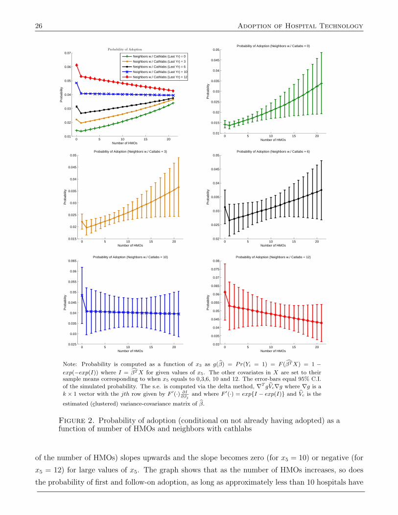
26 Adoption of Hospital Technology
0 5 10 15 200.01
0.02
0.03
0.04
0.05
0.06
0.07Probability of Adoption
Number of HMOs
Pro
babi
lity
Neighbors w./ Cathlabs (Last Yr) = 0
Neighbors w./ Cathlabs (Last Yr) = 3
Neighbors w./ Cathlabs (Last Yr) = 6
Neighbors w./ Cathlabs (Last Yr) = 10
Neighbors w./ Cathlabs (Last Yr) = 12
0 5 10 15 200.01
0.015
0.02
0.025
0.03
0.035
0.04
0.045
0.05Probability of Adoption (Neighbors w./ Catlabs = 0)
Number of HMOs
Pro
babi
lity
0 5 10 15 200.015
0.02
0.025
0.03
0.035
0.04
0.045
0.05Probability of Adoption (Neighbors w./ Catlabs = 3)
Number of HMOs
Pro
babi
lity
0 5 10 15 200.02
0.025
0.03
0.035
0.04
0.045
0.05Probability of Adoption (Neighbors w./ Catlabs = 6)
Number of HMOs
Pro
babi
lity
0 5 10 15 200.025
0.03
0.035
0.04
0.045
0.05
0.055
0.06
0.065Probability of Adoption (Neighbors w./ Catlabs = 10)
Number of HMOs
Pro
babi
lity
0 5 10 15 200.03
0.035
0.04
0.045
0.05
0.055
0.06
0.065
0.07
0.075
0.08Probability of Adoption (Neighbors w./ Catlabs = 12)
Number of HMOs
Pro
babi
lity
Note: Probability is computed as a function of x3 as g(β) = Pr(Yi = 1) = F (βTX) = 1 −exp(−exp(I)) where I = βTX for given values of x5. The other covariates in X are set to theirsample means corresponding to when x5 equals to 0,3,6, 10 and 12. The error-bars equal 95% C.I.
of the simulated probability. The s.e. is computed via the delta method, ∇T gVc∇g where ∇g is a
k × 1 vector with the jth row given by F ′(·) ∂I∂βj
and where F ′(·) = exp{I − exp(I)} and Vc is the
estimated (clustered) variance-covariance matrix of β.
Figure 2. Probability of adoption (conditional on not already having adopted) as afunction of number of HMOs and neighbors with cathlabs
of the number of HMOs) slopes upwards and the slope becomes zero (for x5 = 10) or negative (for
x5 = 12) for large values of x5. The graph shows that as the number of HMOs increases, so does
the probability of first and follow-on adoption, as long as approximately less than 10 hospitals have
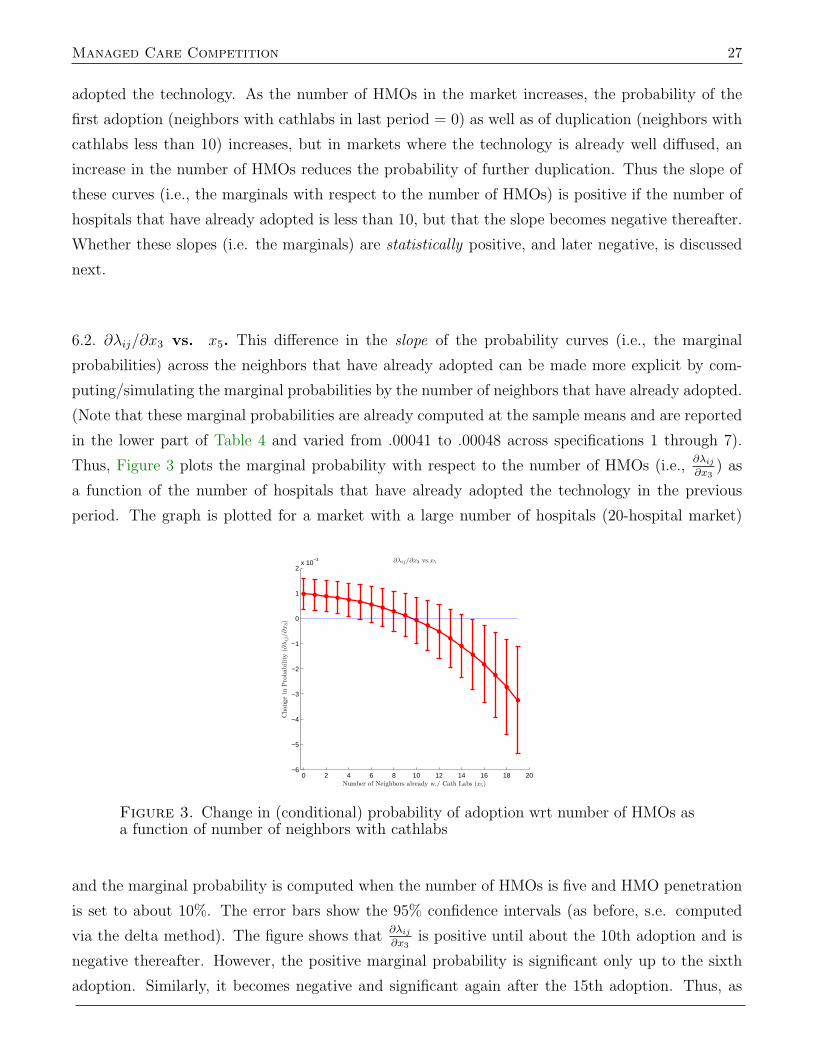
Managed Care Competition 27
adopted the technology. As the number of HMOs in the market increases, the probability of the
first adoption (neighbors with cathlabs in last period = 0) as well as of duplication (neighbors with
cathlabs less than 10) increases, but in markets where the technology is already well diffused, an
increase in the number of HMOs reduces the probability of further duplication. Thus the slope of
these curves (i.e., the marginals with respect to the number of HMOs) is positive if the number of
hospitals that have already adopted is less than 10, but that the slope becomes negative thereafter.
Whether these slopes (i.e. the marginals) are statistically positive, and later negative, is discussed
next.
6.2. ∂λij/∂x3 vs. x5. This difference in the slope of the probability curves (i.e., the marginal
probabilities) across the neighbors that have already adopted can be made more explicit by com-
puting/simulating the marginal probabilities by the number of neighbors that have already adopted.
(Note that these marginal probabilities are already computed at the sample means and are reported
in the lower part of Table 4 and varied from .00041 to .00048 across specifications 1 through 7).
Thus, Figure 3 plots the marginal probability with respect to the number of HMOs (i.e.,∂λij∂x3
) as
a function of the number of hospitals that have already adopted the technology in the previous
period. The graph is plotted for a market with a large number of hospitals (20-hospital market)
0 2 4 6 8 10 12 14 16 18 20−6
−5
−4
−3
−2
−1
0
1
2x 10
−3 ∂λij/∂x3 vs.x5
Number of Neighbors already w./ Cath Labs (x5)
Cha
nge
inP
roba
bilit
y(∂
λij
/∂x3)
Figure 3. Change in (conditional) probability of adoption wrt number of HMOs asa function of number of neighbors with cathlabs
and the marginal probability is computed when the number of HMOs is five and HMO penetration
is set to about 10%. The error bars show the 95% confidence intervals (as before, s.e. computed
via the delta method). The figure shows that∂λij∂x3
is positive until about the 10th adoption and is
negative thereafter. However, the positive marginal probability is significant only up to the sixth
adoption. Similarly, it becomes negative and significant again after the 15th adoption. Thus, as
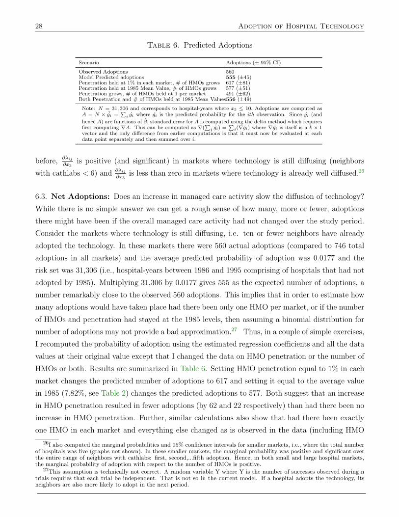
28 Adoption of Hospital Technology
Table 6. Predicted Adoptions
Scenario Adoptions (± 95% CI)
Observed Adoptions 560Model Predicted adoptions 555 (±45)Penetration held at 1% in each market, # of HMOs grows 617 (±81)Penetration held at 1985 Mean Value, # of HMOs grows 577 (±51)Penetration grows, # of HMOs held at 1 per market 491 (±62)Both Penetration and # of HMOs held at 1985 Mean Values556 (±49)
Note: N = 31, 306 and corresponds to hospital-years where x5 ≤ 10. Adoptions are computed asA = N × ¯gi =
∑i gi where gi is the predicted probability for the ith observation. Since gi (and
hence A) are functions of β, standard error for A is computed using the delta method which requiresfirst computing ∇A. This can be computed as ∇(
∑i gi) =
∑i(∇gi) where ∇gi is itself is a k × 1
vector and the only difference from earlier computations is that it must now be evaluated at eachdata point separately and then summed over i.
before,∂λij∂x3
is positive (and significant) in markets where technology is still diffusing (neighbors
with cathlabs < 6) and∂λij∂x3
is less than zero in markets where technology is already well diffused.26
6.3. Net Adoptions: Does an increase in managed care activity slow the diffusion of technology?
While there is no simple answer we can get a rough sense of how many, more or fewer, adoptions
there might have been if the overall managed care activity had not changed over the study period.
Consider the markets where technology is still diffusing, i.e. ten or fewer neighbors have already
adopted the technology. In these markets there were 560 actual adoptions (compared to 746 total
adoptions in all markets) and the average predicted probability of adoption was 0.0177 and the
risk set was 31,306 (i.e., hospital-years between 1986 and 1995 comprising of hospitals that had not
adopted by 1985). Multiplying 31,306 by 0.0177 gives 555 as the expected number of adoptions, a
number remarkably close to the observed 560 adoptions. This implies that in order to estimate how
many adoptions would have taken place had there been only one HMO per market, or if the number
of HMOs and penetration had stayed at the 1985 levels, then assuming a binomial distribution for
number of adoptions may not provide a bad approximation.27 Thus, in a couple of simple exercises,
I recomputed the probability of adoption using the estimated regression coefficients and all the data
values at their original value except that I changed the data on HMO penetration or the number of
HMOs or both. Results are summarized in Table 6. Setting HMO penetration equal to 1% in each
market changes the predicted number of adoptions to 617 and setting it equal to the average value
in 1985 (7.82%, see Table 2) changes the predicted adoptions to 577. Both suggest that an increase
in HMO penetration resulted in fewer adoptions (by 62 and 22 respectively) than had there been no
increase in HMO penetration. Further, similar calculations also show that had there been exactly
one HMO in each market and everything else changed as is observed in the data (including HMO
26I also computed the marginal probabilities and 95% confidence intervals for smaller markets, i.e., where the total numberof hospitals was five (graphs not shown). In these smaller markets, the marginal probability was positive and significant overthe entire range of neighbors with cathlabs: first, second,...fifth adoption. Hence, in both small and large hospital markets,the marginal probability of adoption with respect to the number of HMOs is positive.
27This assumption is technically not correct. A random variable Y where Y is the number of successes observed during ntrials requires that each trial be independent. That is not so in the current model. If a hospital adopts the technology, itsneighbors are also more likely to adopt in the next period.
Managed Care Competition 29
penetration which on average increased from 7.83% to 20.37% over 1985-1995) then the number of
adoptions would have been only 491 (or if penetration is kept at the 1985 level then there would
have been 505 ± 60 adoptions). Thus, the presence of additional HMOs can be associated with 64
additional adoptions. Finally, the net impact of HMOs, due to an increase in both the number of
HMOs and HMO penetration can be judged by holding these variables to their 1985 values. Doing
so results in 556 adoptions. Note that this value is not very far from the true predicted value of 555,
suggesting that the net impact of HMO activity on the adoption of cathlabs has been very small.28
7. Summary
Managed care organizations change the incentives faced by health care providers which in turn
can have significant implications for the diffusion of technology. This paper finds that an increase
in HMO penetration is associated with a slower diffusion of cardiac catheterization laboratories.
However, an increase in HMO competition (whether measured as the number of HMOs, HMOs per
capita or by the Herfindahl index) has a countervailing effect in that it increases the probability of
adoption.
The results can be understood in the context of bargaining between HMOs and hospitals. A
monopoly HMO can obtain large discounts from hospitals which in turn reduces the profitability
of the hospitals and slows diffusion of expensive technologies. As the number of HMOs increases,
their bargaining position weakens, resulting in lower discounts by hospitals. However, this latter
effect is non-linear and arises due to an inherent trade-off in the expected volume of a hospital when
additional hospitals join the HMO’s network: If the network is small, each hospital in the network
gets a larger share of the HMO enrollees who use the network hospitals but if the network is large,
while each hospital gets a smaller share of the enrollees, more enrollees receive services from network
hospitals.
Simulations for cathlabs show that when there are relatively few neighbors that have adopted the
technology, an increase in the number of HMOs increases the probability of adoption but when many
have already adopted the technology, the effect of the number of HMOs is the opposite. However,
28These estimates are very rough since no corrections are made to account for the fact that the adoptions are not trulyindependent: If one less hospital adopts in a market due to fewer HMOs then in the next period the neighboring hospitalswould have one less neighbor with the technology, and hence the total probability of adoption for each of the neighbors wouldfurther decrease. The second order corrections to the estimate can be made as follows: Separate the data by years and foreach year generate Bernoulli outcomes (1 for adoption and 0 for non-adoption) with the probability of success p given bythe scenario. Next, for each year, count the number of neighbors that have cathlabs (i.e., the Bernoulli successes plus thenumber of adopters in 1985). Use this figure to recompute the number of neighbors with catheterization laboratories in theprevious year and then simulate to estimate the new probability of adoption. This approach was not taken due to the highcost of computing time: In order to compute how many of the neighbors have adopted the technology, a n × n matrix mustbe created for every year where the i,j entry of the matrix (a 1 or a 0) indicates if j is a neighbor to i and n is the numberof hospitals in the U.S. in that year. This matrix must then by multiplied with a n × 1 vector which indicates that the ith.hospital has a catheterization laboratory. The matrix multiplication provides the number of neighbors that a hospital has withcatheterization laboratory. This method was used in the main analysis to compute the number of neighbors and neighborswith catheterization laboratories (each year) and took the bulk of the computing time.

30 Adoption of Hospital Technology
the effect of penetration is always to reduce the adoption probability. Thus, when technology is still
diffusing (i.e. is relatively rare) competition and penetration work in opposite directions and the
net effect could be positive or negative. In fact, when penetration and number of HMOs at held at
their 1985 values, the predicted number of adoptions is the same as the actual observed number of
adoptions. While these are only simulations, they do suggest why the prior literature, which has
ignored the competition effect, has sometimes reported mixed results on HMO penetration. The
results are robust for the case of cardiac catheterization laboratories, however, it would be useful
to check them for other important hospital technologies – choosing some that had not yet well
diffused over the period when HMO penetration and competition were increasing and others that
were already (relatively) well diffused.

Managed Care Competition 31
Appendix A
This appendix derives the optimal bid given in equation (3) on page 7.
Basic setup: There are K non-network hospitals. For all hospitals, the unit price of service is 1,
unit cost is ci ∼ U [0, 1] and is iid. The distribution is known by all but the realization of ci is known
only to the hospital. The jth HMO is soliciting discount bids from these K hospitals. The bidder
with the largest discount d is added to the jth HMO’s network such that the size of the network
increases from Gj to Gj + 1. Also, γj is the parameter that measures the control of the HMO to
restrict its enrollees to use in-network hospitals. Thus, γj = 1 means that with probability 1, an
enrollee will use one of the Gj + 1 in-network hospitals and if γj = (Gj + 1)/(Gj + K) then the
HMO has no control over its enrollees and an enrollee will visit any of the Gj + K hospitals with
equal probability. Thus, the ith hospital’s problem is to find d∗i such that the expected profit is
maximized, i.e.,
maxdi
((1− di − ci)
γjSjGj + 1
− α)
Pr(di > d∗(ck) ∀k 6= i)
+((1− ci)
(1− γj)SjK − 1
− α)(1− Pr(·))
(A-1)
Solution: Assume that d∗, if it exists, is monotonic and decreasing in ci (decreasing because hospitals
are bidding a discount below the price of 1) and then verify that the solution is indeed monotonically
decreasing in ci. Envision that the way the bidding will take place is that the bidder will pretend
that his unit cost is some value r and will bid according to the discount bid function with the value
of r. Then the problem reduces to maximizing the objective function given above over r. Thus,
hospital i will win the bid with probability
Pr(d∗(r) > d∗(ck) ∀ k 6= i)→ Pr(r < ck ∀ k 6= i). (A-2)
For any one given ck, let Pr(r < ck) = 1− Pr(ck < r) = 1− F (r). Then, due to the independence
assumption of ck, Pr(r < ck ∀ k 6= i) = (1− F (r))(K−1). Rewriting the last probability as ρ(r), the
maximization problem is just
maxr
(1− di − ci)γjSjGj + 1
ρ(r) + (1− ci)(1− γj)SjK − 1
(1− ρ(r))− α. (A-3)
From the FOCs we get
∂(Obj Fn)/∂r = 0
⇒ (1− d∗(r)− ci)γjSj(Gj + 1)
ρ′(r)− d′∗(r) γjSj(Gj + 1)
ρ(r)− ρ′(r)(1− ci)(1− γj)Sj(K − 1)
= 0
⇒ γjSjGj + 1
{d∗(r)ρ′(r) + d′∗(r)ρ(r)
}= (1− ci)ρ′(r)
γjSjGj + 1
− (1− ci)ρ′(r)(1− γj)Sj(K − 1)
⇒ γj(Gj + 1)
∂
∂r{d∗(r)ρ(r)} = (1− ci)ρ′(r)
[ γjGj + 1
− 1− γjK − 1
](A-4)

32 Adoption of Hospital Technology
In order to solve for d∗, we use the fact that in equilibrium we must have r = ci, integrate from ci
to 1 and use the boundary condition that d∗(1) = 0. Thus,
γj(Gj + 1)
∫ 1
ci
∂
∂t{d∗(t)ρ(t)}dt =
−γj(G+ 1)
ρ(ci)d∗(ci) (A-5)
which gives
d∗(ci) = −(Gj + 1)
γjρ(ci)
{∫ 1
ci
(1− t)ρ′(ci)[ γjGj + 1
− 1− γjK − 1
]}dt. (A-6)
In order to integrate, note that ρ′(r) = (K − 1)(1 − F (r))(K−2)(−f(r)) and ci ∼ U [0, 1] (and iid),
so F (r) = r and f(r) = 1. Thus,
ρ(ci) = (1− ci)(K−1)
and ρ′(ci) = (K − 1)(1− ci)(k−2)(−1)(A-7)
and substituting these back in the expression for d∗(ci) above, we get
d∗(ci) = −(Gj + 1)(K − 1)
γjρ(ci)
[ γjGj + 1
− 1− γjK − 1
]{ ∫ 1
ci
(1− t)(1− t)(K−2)(−1)dt}
= −(Gj + 1)(K − 1)
γj(1− ci)(K−1)
[ γjGj + 1
− 1− γjK − 1
]{ ∫ 1
ci
(1− t)(K−1)(−1)dt} (A-8)
which simplifies to
d∗(ci) =(1− ci)K
((K − 1)− (1− γj)(Gj + 1)
γj
). (A-9)
Note that Sorensen’s (2003) result is reproduced for Gj = 0, K = 2.
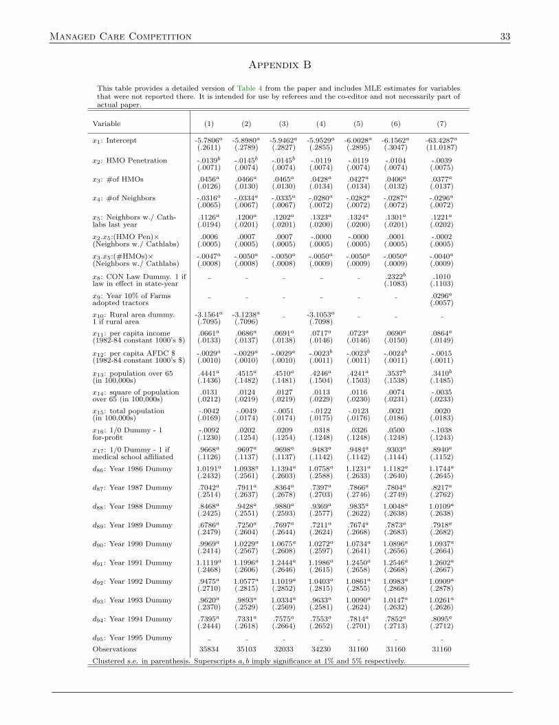
Managed Care Competition 33
Appendix B
This table provides a detailed version of Table 4 from the paper and includes MLE estimates for variablesthat were not reported there. It is intended for use by referees and the co-editor and not necessarily part ofactual paper.
Variable (1) (2) (3) (4) (5) (6) (7)
x1: Intercept -5.7806a -5.8980a -5.9462a -5.9529a -6.0028a -6.1562a -63.4287a
(.2611) (.2789) (.2827) (.2855) (.2895) (.3047) (11.0187)
x2: HMO Penetration -.0139b -.0145b -.0145b -.0119 -.0119 -.0104 -.0039(.0071) (.0074) (.0074) (.0074) (.0074) (.0074) (.0075)
x3: #of HMOs .0456a .0466a .0465a .0428a .0427a .0406a .0377a
(.0126) (.0130) (.0130) (.0134) (.0134) (.0132) (.0137)
x4: #of Neighbors -.0316a -.0334a -.0335a -.0280a -.0282a -.0287a -.0296a
(.0065) (.0067) (.0067) (.0072) (.0072) (.0072) (.0072)
x5: Neighbors w./ Cath- .1126a .1200a .1202a .1323a .1324a .1301a .1221a
labs last year (.0194) (.0201) (.0201) (.0200) (.0200) (.0201) (.0202)
x2.x5:(HMO Pen)× .0006 .0007 .0007 -.0000 -.0000 .0001 -.0002(Neighbors w./ Cathlabs) (.0005) (.0005) (.0005) (.0005) (.0005) (.0005) (.0005)
x3.x5:(#HMOs)× -.0047a -.0050a -.0050a -.0050a -.0050a -.0050a -.0040a
(Neighbors w./ Cathlabs) (.0008) (.0008) (.0008) (.0009) (.0009) (.0009) (.0009)
x8: CON Law Dummy. 1 if .2322b .1010law in effect in state-year (.1083) (.1103)
x9: Year 10% of Farms .0296a
adopted tractors (.0057)
x10: Rural area dummy. -3.1564a -3.1238a -3.1053a
1 if rural area (.7095) (.7096) (.7098)
x11: per capita income .0661a .0686a .0691a .0717a .0723a .0690a .0864a
(1982-84 constant 1000’s $) (.0133) (.0137) (.0138) (.0146) (.0146) (.0150) (.0149)
x12: per capita AFDC $ -.0029a -.0029a -.0029a -.0023b -.0023b -.0024b -.0015(1982-84 constant 1000’s $) (.0010) (.0010) (.0010) (.0011) (.0011) (.0011) (.0011)
x13: population over 65 .4441a .4515a .4510a .4246a .4241a .3537b .3410b
(in 100,000s) (.1436) (.1482) (.1481) (.1504) (.1503) (.1538) (.1485)
x14: square of population .0131 .0124 .0127 .0113 .0116 .0074 -.0035over 65 (in 100,000s) (.0212) (.0219) (.0219) (.0229) (.0230) (.0231) (.0233)
x15: total population -.0042 -.0049 -.0051 -.0122 -.0123 .0021 .0020(in 100,000s) (.0169) (.0174) (.0174) (.0175) (.0176) (.0186) (.0183)
x16: 1/0 Dummy - 1 -.0092 .0202 .0209 .0318 .0326 .0500 -.1038for-profit (.1230) (.1254) (.1254) (.1248) (.1248) (.1248) (.1243)
x17: 1/0 Dummy - 1 if .9668a .9697a .9698a .9483a .9484a .9303a .8940a
medical school affiliated (.1126) (.1137) (.1137) (.1142) (.1142) (.1144) (.1152)
d86: Year 1986 Dummy 1.0191a 1.0938a 1.1394a 1.0758a 1.1231a 1.1182a 1.1744a
(.2432) (.2561) (.2603) (.2588) (.2633) (.2640) (.2645)
d87: Year 1987 Dummy .7042a .7911a .8364a .7397a .7866a .7804a .8217a
(.2514) (.2637) (.2678) (.2703) (.2746) (.2749) (.2762)
d88: Year 1988 Dummy .8468a .9428a .9880a .9369a .9835a 1.0048a 1.0109a
(.2425) (.2551) (.2593) (.2577) (.2622) (.2638) (.2638)
d89: Year 1989 Dummy .6786a .7250a .7697a .7211a .7674a .7873a .7918a
(.2479) (.2604) (.2644) (.2624) (.2668) (.2683) (.2682)
d90: Year 1990 Dummy .9969a 1.0229a 1.0675a 1.0272a 1.0734a 1.0896a 1.0937a
(.2414) (.2567) (.2608) (.2597) (.2641) (.2656) (.2664)
d91: Year 1991 Dummy 1.1119a 1.1996a 1.2444a 1.1986a 1.2450a 1.2546a 1.2602a
(.2468) (.2606) (.2646) (.2615) (.2658) (.2668) (.2667)
d92: Year 1992 Dummy .9475a 1.0577a 1.1019a 1.0403a 1.0861a 1.0983a 1.0909a
(.2710) (.2815) (.2852) (.2815) (.2855) (.2868) (.2878)
d93: Year 1993 Dummy .9620a .9893a 1.0334a .9633a 1.0090a 1.0147a 1.0261a
(.2370) (.2529) (.2569) (.2581) (.2624) (.2632) (.2626)
d94: Year 1994 Dummy .7395a .7331a .7575a .7553a .7814a .7852a .8095a
(.2444) (.2618) (.2664) (.2652) (.2701) (.2713) (.2712)
d95: Year 1995 Dummy
Observations 35834 35103 32033 34230 31160 31160 31160
Clustered s.e. in parenthesis. Superscripts a, b imply significance at 1% and 5% respectively.

34 Adoption of Hospital Technology
References
Acemoglu, Daron and Amy Finkelstein, “Input and technology choices in regulated industries:Evidence from the health care sector,” NBER Working Paper 12254, National Bureau of EconomicResearch May 2006.
Ambrus, Attila and Rossella Argenziano, “Asymmetric networks in two-sided markets,” June2006.
American Heart Association, 2000 Heart and stroke statistical update 1999. Dallas, Tex.: Amer-ican Heart Association, 1999.
Baker, Laurence C., “The Effect of HMOs on Physician Practices,” August 1996. StanfordUniversity (mimeo).
, “Manged care and technology adoption in health care: Evidence from magnetic resonanceimaging,” Journal of Health Economics, May 2001, 20 (3), 395421.
and Ciaran S. Phibbs, “Managed care, technology adoption, and health care: Theadoption of neonatal intensive care,” RAND Journal of Economics, Autumn 2002, 33 (3), 524–548.
and Joanne Spetz, “Managed care and medical technology growth,” NBER WorkingPaper 6894, National Bureau of Economic Research, Cambridge, MA January 1999.
and Martin L. Brown, “The effects of managed care on health care providers,” NBERWorking Paper 5987, National Bureau of Economic Research April 1997.
and , “Managed care, consolidation among health care providers, and health care:Evidence from mammography,” RAND Journal of Economics, Summer 1999, 30 (2), 351–374.
Baumgardner, James R., “The Interaction Between Forms of Insurance Contract and Types ofTechnical Change in Medical Care,” RAND Journal of Economics, Spring 1991, 22 (1), 36–53.
Capps, Cory, David Dranove, and Mark Satterthwaite, “Competition and market power inoption demand markets,” RAND Journal of Economics, September 2003, 34 (4), 737–763.
Consumer Reports, “High-tech competition: the cardiac money machine,” Consumer Reports,July 1992, pp. 446–47.
Cragg, J.G., “More efficient estimation in the presence of heteroskedasticity of unknown form,”Econometrica, May 1983, 51 (3), 751–764.
Cutler, David M. and Mark McClellan, “The determinants of technological change in heart at-tack treatment,” NBER Working Paper 5751, National Bureau of Economic Research September1996.
and , “Is technological change in medicine worth it?,” Health Affairs, Septem-ber/October 2001, 20 (5), 11–29.
Davidson, Russell and James G. Mackinnon, Econometric Theory and Methods, Oxford:Oxford University Press, 2004.
Dranove, David, Anne Gron, and Michael J. Mazzeo, “Differentiation and competition inHMO markets,” Journal of Industrial Economics, December 2003, 51 (4), 433–454.
, Mark Shanley, and Carol Simon, “Is hospital competition wasteful?,” RAND Journalof Economics, Summer 1992, 23 (2), 247–262.
Fudenberg, Drew and Jean Tirole, “Preemption and rent equilization in the adoption of newtechnologuy,” Review of Economic Studies, July 1985, 52 (3), 383–401.
Gaynor, Martin and William B. Vogt, “Competition among hospitals,” Rand Journal ofEconomics, 2003, 34 (4), 764–785.
Gaynor, Martin S. and Deborah Haas-Wilson, “Change, consolidation and competition inhealth care markets,” Journal of Economic Perspectives, Winter 1999, 13 (1), 141–164.
Gowrisankaran, Gautam, “Productivity in heart attack treatments,” Economic Letter 20, Fed-eral Reserve Bank of San Francisci 2002.
Griliches, Zvi, “Hybrid Corn: An exploration in the econometrics of technological change,” Econo-metrica, October 1957, 25 (4), 501–522.
Hamilton, Barton H. and Brian McManus, “Technology diffusion and market structure:Evidence from infertility treatment markets,” September 2005.
Heidenreich, P. and Mark McClellan, “Trends in treatment and outcomes for acute myocardial

Managed Care Competition 35
infarction: 19751995,” American Journal of Medicine, 2001, 110 (3), 165–174.Hodgkin, Dominic, “Specialized service offerings and patients’ choice of hospital: The case of
cardiac catheterization,” Journal of Health Economics, 1996, 15, 305–332.Joskow, Paul, Controlling Hospital Costs: The Role of Government Regulation, Cambridge: MIT
Press, 1981.Luft, Harold S., James C. Robinson, Deborah W. Garnick, and Susan C. Maerki, “The
role of specialized clinical services in competition among hospitals,” Inquiry, Spring 1986, 23 (1),83–94.
Makuc, Diane, Bengt Hagland, Deborah D. Ingram, Joel C. Kleinmann, and Jacob J.Feldman, “The use of health service areas for measuring provider availability,” The Journal ofRural Health, Supplemental 1991, 7 (4), 347–356.
, Bengt Haglund, Deborah D. Ingram, Joel C. Kleinman, and Jacob J. Feldman,“Health services areas for the United States,” in “Vital and Health Statistics; Data evaluationand methods research,” Vol. 2(112), Hyattsville, MD: U.S. Department of Health and HumanServices, National Center for Health Statistics, November 1991.
Meyer, Bruce D., “Unemployment insurance and unemployment spells,” Econometrica, July1990, 58 (4), 757–782.
Newhouse, Joseph P., “Medical care costs: How much welfare loss?,” Journal of EconomicPerspectives, Summer 1992, 6 (3), 3–21.
Ohsfeldt, Robert L, Michael A Morrisey, Leonard Jack Nelson, and Victoria Johnson,“The Spread of State Any Willing Provider Laws,” Health Services Research, 1998, 33 (5), 1537–1562.
Pauly, Mark V., “Managed care, market power, and monopsony,” Health Services Research,December 1998, 33 (5), 1439–1460.
Prentice, Ross L. and L.A. Gloeckler, “Regression analysis of grouped survival data withapplication to breast cancer data,” Biometrics, March 1978, 34, 57–67.
Putnam, Robert D., “Bowling alone: America’s declining social capital,” Journal of Democracy,1995, 6 (1), 65–78.
, Bowling alone: the collapse and revival of American community, Simon & Schuster, 2000.Rapoport, John, “Diffusion of technological innovation among nonprofit firms: A case study of
radioisotopes in the U.S. hospitals,” Journal of Economics and Business, 1978, 30, 108–118.Reinganum, Jennifer F., “On the diffusion of new technology: A game theoretic approach,”
Review of Economic Studies, July 1981, 48 (3), 395–405., “The timing of innovation: Research, development, and diffusion,” in R. Schmalensee and
R.D. Willig, eds., Handbook of Industrial Organization, Vol. 1, North-Holland: Elsevier ScienceB.V., 1989.
Robinson, James C. and Harold S. Luft, “Competition and the cost of hospital care, 1972 to1982,” Journal of the American Medical Association, June 19 1987, 257 (23), 3241–3245.
, , Stephen J. McPhee, and Sandra S. Hunt, “Hospital competition andsurgical length of stay,” Journal of the American Medical Association, February 5 1988, 259 (5),696–700.
Rose, Nancy L. and Paul L. Joskow, “The diffusion of new technologies: evidence from theelectric utility industry,” RAND Journal of Economics, Autumn 1990, 21 (3), 354–373.
Salkever, D.C. and T.W. Bice, “The impact of Certificate of Need controls on hospital invest-ment,” Milbank Fund Memorial Quarterly, 1976, 54, 185–214.
Schmidt-Dengler, Philipp, “The timing of new technology adoption: The case of MRI,” June2006.
Sheils, John F., David C. Stapleton, and Randall Haught, “The Cost of Legislative Re-strictions on Contracting Practices: The Cost to Governments, Employers, and Families,” 1995.Report prepared by Lewin-VHI.
Shen, Yu-Chu, Vivian Wu, and Glenn Melnick, NBER Working Paper 13775, NationalBureau of Economic Research February 2008.
Skinner, Jonathan and Douglas Staiger, “Technology adoption from hybrid corn to betablockers,” NBER Working Paper 11251, National Bureau of Economic Research March 2005.
36 Adoption of Hospital Technology
Sloan, F.A. and B. Steinwald, “Effects of regulation on hospital costs and input use,” Journalof Law and Economics, 1980, 23 (1), 81–110.
Sloan, Frank A., Michael A. Morrisey, and Joseph Valvona, “Medicare prospective paymentand the use of medical technologies in hospitals,” Medical Care, September 1988, 26 (9), 837–853.
Sorensen, Alan T., “Insurer-hospital bargaining: Negotiated discounts in post-deregulation Con-necticut,” The Journal of Industrial Economics, December 2003, 51 (4), 469–490.
Vogt, William B., “Preemptive technology adoption: The example of magnetic resonance imag-ing,” November 1998. Unpublished (mimeo).
Welch, W.P., “The elasticity of demand for health maintenance organizations,” Journal of HumanResources, Spring 1986, 21 (2), 252–266.
Wholey, Douglas, Roger Feldman, and Jon B. Christianson, “The effect of market structureon HMO premiums,” Journal of Health Economics, 1995, 14 (1), 81–105.
Wooldridge, Jeffrey M., Econometric analysis of cross section and panel data, Cambridge: MITPress, 2002.