1

Making SAS® the Easy Way Out:

Harnessing the Power of PROC TEMPLATE to Create Reproducible, Complex Graphs Debra A. Goldman, Memorial Sloan Kettering Cancer Center, New York, NY

ABSTRACT

With high pressure deadlines and mercurial collaborators, creating graphs in the most familiar way seems like the best option. Using post-processing programs like Photoshop or Microsoft Powerpoint to modify graphs is quicker and easier to the novice SAS® User or for one’s collaborators to do on their own. However, reproducibility is a huge issue in the scientific community. Any changes made outside statistical software need to be repeated when collaborator preferences change, the data changes, the journal requires additional elements, and a host of other reasons The likelihood of making errors increases along with the time spent making the figure. Learning PROC TEMPLATE allows one to seamlessly create complex, automatically generated figures and eliminates the need for post-processing.

This paper demonstrates how to do complex graph manipulation procedures in SAS 9.3

or later to solve common problems, including lattice panel plots for different variables, split plots and broken axes, weighted panel plots, using select observations in each panel, waterfall plots, and graph annotation. The examples presented are healthcare based, but the methods are applicable to finance, business and education. Attendees should have a basic understanding of the macro language, graphing in SAS using SGPLOT, and ODS graphics.

INTRODUCTION

SGPLOT and SGPANEL are powerful graphing tools that can accomplish most of one’s graphing needs. These procedures are written for a standard dataset and a logical coding mind. However, in my experience, not every graphical request follows the conventions of traditional coding. I’ve found the capabilities of standard plotting procedures are limited in situations such as:

• Putting multiple graphs with different variables on the same lattice panel • Using only select observations within each series or graph • Splitting a plot to zoom in / reduce white space • Creating a broken axis • Annotating Kaplan Meier plots • Creating a waterfall plot with a specific bar width • Creating a panel plot with each plot being a different size

Prior to learning PROC TEMPLATE and the graph template language (GTL), honestly, it was easier use post processing procedures, like Photoshop, to combine plots or to use other statistical software. I know PROC TEMPLATE can seem like an insurmountable feat. The syntax is slightly different, leading to frequent initial errors, and, the extensive options available make narrowing in on the correct one seem like searching for a needle in a haystack. Further, in some instances, there are multiple ways of accomplishing the same goal.

My goal is to provide a guide for how to solve some common complex graphing

problems using PROC TEMPLATE. I’ll go through examples for how to solve the issues listed above. The examples here will be medically based as that’s where my expertise lies, but these concepts can easily be extended to business, finance, and education. Readers should be familiar with the basic conversion of SGPLOT and SGPANEL commands to PROC TEMPLATE commands, for which I recommend the following introduction1, and readers should also have some experience with the SAS MACRO language.

2

KEYWORDS GTL, PROC TEMPLATE, EVAL(IFN()), MACRO, SPLIT PLOT, BROKEN AXIS, PANEL WITH WEIGHTS, WATERFALL PLOT, ANNOTATE, KAPLAN MEIER PLOT EXAMPLE 1: SIMPLE LATTICE PANEL FOR FIGURES WITH DIFFERENT VARIABLES

PROC SGPANEL allows one to put multiple plots within the same panel using the PANELBY command. This is great when one has the same x and y axis variables, and grouping variables. However, there are certainly instances where one needs to use different variables, such as multiple surgical outcomes, separate survival outcomes and stratification variables, and different radiotracers. Additionally, particular to medicine and science, some journals have limits on the number of graphs, but not on the number of plots that can be placed in one graph panel. It’s possible using ODS Graphics to put different graphs from SGPLOT within the same word or PDF document, but most journals require graphs in graphical formats, such as .jpg, tiff, or .png.

Fortunately, PROC TEMPLATE makes it easy to do this using the LAYOUT LATTICE

command, which creates a panel for graphs, followed by the LAYOUT OVERLAY command, which allows different plot functions to be laid on top of one another in the same plot. For a discussion on the difference between LAYOUT DATALATTICE versus LAYOUT LATTICE or LAYOUT GRRIDED, please see the Graph Template Language Documentation, starting on page 292. Personally, I’ve found LAYOUT LATTICE to be sufficient for all of my PROC TEMPLATE graphing needs. For this example, we’ll use the following dataset containing surgery characteristics on 7 consecutive cohorts of 20 patients: Example 1 Dataset found in Appendix When I initially worked on this project, I sent the investigator four separate plots for each surgery outcome. After a few months, they sent back a Microsoft PowerPoint with of all these plots on the same slide labeled “A”,”B”,”C”, and “D,” and asked me to combine the graphs into one plot. They also asked for some formatting changes and consistency among the graphs. I used PROC TEMPLATE with a MACRO for each series to complete my goal, similar to the example in Pratt’s paper1. STEP 1. GENERATE LATTICE TEMPLATE proc template; define statgraph example1_template_v1 ; begingraph /designwidth=1000px designheight=1000px; layout lattice/ COLUMNS =2 ROWS=2 ; rowheaders; entry "A. " /textattrs=(size=16pt weight=bold) pad=5pt ; entry "C. " /textattrs=(size=16pt weight=bold) pad=5pt; endrowheaders; row2headers; entry "B. " /textattrs=(size=16pt weight=bold) pad=5pt; entry "D. " /textattrs=(size=16pt weight=bold) pad=5pt; endrow2headers; rowaxes; rowaxis / griddisplay=on; endrowaxes; /*MACRO CODE WILL GO IN HERE*/ endlayout; endgraph; end; run; quit;

3

SAS Syntax Meaning define statgraph Creates the template. After this command, enter the

name of your graph designwidth Width of your graph; “px” refers to pixels and “in” refers to

inches designheight Height of your graph COLUMNS Number of Columns ROWS Number of Row s

Rowheaders / endrowheaders Side panel t it les for each of the graphs. Number follow ing statement, such as “2” above indicates the second row

Entry " " Creates the row header. Value w ithin quotes after entry is the t itle of the row header

Rowaxes/ endrowaxes Defines a shared row axis; Table 1a. Definition “Cheat Sheet” for Example 1 Template STEP 2. CREATE MACRO FOR REPEAT GRAPHS The SAS MACRO language is fantastic for reducing the length of one’s code and for making it easy to update a feature present in multiple components of one’s analysis. I usually start by deciding what’s consistent about the plots and what should be different. Any of the consistent items should be hard coded into the macro. Any differences should be macro variables.

• Are the y-axes the same? If not, do the axis values change? Labels? • Are the x-axes the same? If not, do the axis values change? Labels? • Do the graphs each have a different title? • Is the same y-variable being used throughout? • Is the same x-variable used throughout? • Should the colors or markers change?

Note: if the reader is uncomfortable with the SAS MACRO language, all one needs to do is take the syntax out of the macro, replace all macro variables with hard coded variables, and paste into the template. %macro seriesplot (cellheader_label=,yvar=,xvar=,ylabel=,xlabel=,yviewmin=,yviewmax=); cell ; layout overlay / yaxisopts=(display=all griddisplay=auto_on label=&ylabel LABELATTRS=( size=13 family="Arial") labelfitpolicy=split linearopts=(viewmin=&yviewmin viewmax=&yviewmax) tickvalueattrs=(size=11pt family="Arial")) xaxisopts= (label=&xlabel discreteopts=(tickvaluefitpolicy=ROTATEALWAYS) LABELATTRS=( size=13 family="Arial") GRIDATTRS=(thickness=10) labelfitpolicy=split tickvalueattrs=(size=11pt family="Arial")) border=true borderattrs=(thickness=1); /*creates the series plot for the median */ seriesplot x=&xvar y=&yvar._median / curvelabel="Median" curvelabellocation=outside datalabel=&yvar._median datalabelattrs=(size=11) markerattrs=(symbol=circlefilled) curvelabelattrs=(size=12) display=all; /*creates the series plot for the 25th percentile */ seriesplot x=&xvar y=&yvar._q1 / curvelabel="25th %" curvelabellocation=outside datalabel=&yvar._q1 datalabelattrs=(size=11) markerattrs=(symbol=circlefilled) curvelabelattrs=(size=12) display=all; /*creates the series plot for the 75th percentile*/ seriesplot x=&xvar y=&yvar._q3 / curvelabel="75th %" curvelabellocation=outside datalabel=&yvar._q3 datalabelattrs=(size=11) markerattrs=(symbol=circlefilled) curvelabelattrs=(size=12) display=all; /*puts a band plot between the 25th and 75th percentile*/

4

bandplot x=&xvar limitupper=&yvar._q3 limitlower=&yvar._q1 / fillattrs=(transparency=0.5) ; endlayout; endcell; %mend seriesplot; SAS Syntax Meaning Cell / endcell Init iates the cell in the panel matrix for the plot. Cells f ill

the row first and then proceed to the next column Yaxisopts= Sets the y ax is options Viewmin= Sets the minimum value of the axis Viewmax= Sets the maximum value of the axis Label= Labels the axis Discreteopts=() Tells SAS how to handle discrete values Tickvaluefitpoilicy= Tells SAS how to handle tic k marks that overlap Labelfitpolicy= Tells SAS how to handle labels that are long or that

intersect Tickvalueattrs=() Provides the attributes for the t ick marks Borderattrs= Indicates the attr ibutes for the border of the cell Layout overlay Provides the layout for the cell. Overlay tell SAS to

overlay all the plot commands Border=true Tells SAS to create a border around the cell Seriesplot Creates a series plot, w hich connects specif ied marker

points w ith a line Curvelabel Labels the series Curvelabelattrs=() Sets the attributes of the label Curvelabellocation= Sets the location of the label Datalabel Defines the variable used to label the data points Datalabelattrs=() Sets the attributes of the data point labels

Display= Indicates w hether to display all data labels or to truncate when any intersect

bandplot Creates a band plot, w hich overlays on the series. It shades in the portion betw een the 25th and 75th percentile here

Fillattrs=(transparency=) Indicates the transparency of the band Table 1b. Definition “Cheat Sheet” for Example 1 Macro Advanced Move: In SAS Macro language, the “.” Serves as a delineator between the macro variable name and the remaining code. As all these variables have the same prefix, I used the “.” to reduce the number of macro variables needed to pass through. It’s not necessary, but one may find this useful in other macro scenarios as well STEP 3. ADD THE MACRO COMMAND TO THE TEMPLATE LANGUAGE proc template; define statgraph example1_template_v2 ; begingraph /designwidth=1000px designheight=1000px; layout lattice/COLUMNS=2 rows=2 ; rowheaders ; entry "A. " /textattrs=(size=16pt weight=bold) pad=5pt ; entry "C. " /textattrs=(size=16pt weight=bold) pad=5pt; endrowheaders; row2headers; entry "B. " /textattrs=(size=16pt weight=bold) pad=5pt; entry "D. " /textattrs=(size=16pt weight=bold) pad=5pt; endrow2headers; rowaxes; rowaxis / griddisplay=on; endrowaxes; %seriesplot(yvar=est_bloodloss,xvar=cohort,ylabel="Estimated Blood Loss (cc)", xlabel="Consecutive Patient Cohort", yviewmin=100 ,yviewmax=700);

5

%seriesplot(yvar=optime,xvar=cohort,ylabel="Operating Time (min)", xlabel="Consecutive Patient Cohort", yviewmin=500, yviewmax=1300); %seriesplot(yvar=total_ln,xvar=cohort,ylabel="Total # LN Harvested", xlabel="Consecutive Patient Cohort", yviewmin=0, yviewmax=45); %seriesplot(yvar=los,xvar=cohort,ylabel="Length of Stay (days)", xlabel="Consecutive Patient Cohort", yviewmin=0, yviewmax=20); endlayout; endgraph; end; run; quit; STEP 4: RUN USING PROC SGRENDER /*formats the values in a coded column*/ proc format; value cohortf 1="1-20" 2="21-40" 3="41-60" 4="61-80" 5="81-100" 6="101-120" 7="121-140"; run; proc sgrender template=example1_template_v2 data=example1_surgerychar; format cohort cohortf.; run;

Output 1. Plot for Example 1. Style=sasweb EXAMPLE 2: SPLIT PLOTS USING EVAL(IFN()) AND BROKEN AXES PLOTS

Example 1 demonstrated how to use the lattice feature to create a panel plot for multiple graphs with different variables, a simple introduction to PROC TEMPLATE. Even in the situation where one has only one plot to make, PROC TEMPLATE can be used to enhance and

6

customize the graph. When one needs to select only certain observations from a dataset, one can use the EVAL(IFN() statement to subset. For this example, we’ll use a dataset which contains the annual proportion of time the Gastric and Hepatopancreatobiliary (HPB) services used Operating Room 1 and Operating Room 2 from 2000-2010: Example 2 dataset found in Appendix I initially used Proc SGplot as follows to make the graph: proc sgplot data=example2_proptime pctlevel=graph; series x= year y = days_prop/ group=days_label datalabel=days_prop markers; yaxis values = (10 to 45) label="% Days / Total Days" offsetmin=0 labelattrs=(weight=bold); xaxis type=discrete offsetmax=0.1 offsetmin=0.1 labelattrs=(weight=bold); keylegend /title=""; run;

Output 2a. Initial graph using SGPLOT After seeing the above plot, the investigator had three concerns. First, they felt the white space was unnecessary and masking the individual time trends in the series with the lower proportions. Second, we knew from the data that the lower proportion series did not overlap or crisscross as suggested by this plot. Third, the investigator wanted the labels for the last curve to be on the bottom consistently, rather than the top of the line. To remove the white space, enhance the trends in the bottom two series, and to use unique positioning for the data labels, I used PROC TEMPLATE with an EVAL(IFN()) statement to enhance the graph. EVAL invokes the macro function to evaluate the statement provided prior to compiling the procedure. IFN invokes the macro function to use an if-then statement. Ifn(condition to be met, value when true, value when false) Using this I could put these four series in two separate plots, one for the two larger proportions and one for the two smaller proportions, with two separate axis values. Further, I could use the ROWAXIS feature and COLUMNAXIS feature to put these plots on the same plane and reduce the white space.

7

STEP 1: GENERATE THE TEMPLATE proc template; define statgraph example2a_template; begingraph /designwidth=5in designheight=4in; layout lattice/COLUMNS=1 rows=2 rowgutter=0pt columngutter=0pt columndatarange=union ; columnaxes; columnaxis / griddisplay=on label="Year" linearopts=(viewmin=2000 viewmax=2010) LABELATTRS=( size=13 family="Arial" weight=bold) tickvalueattrs=(size=11pt family="Arial") type=discrete offsetmax=0.1 offsetmin=0.1; endcolumnaxes; rowaxes; rowaxis / griddisplay=on label="% Service Days /Total Days" LABELATTRS=( size=13 family="Arial" weight=bold) tickvalueattrs=(size=11pt family="Arial"); endrowaxes; cell ; layout overlay / yaxisopts=(display=all label="% Service Days /Total Days" griddisplay=auto_on tickvalueattrs=(size=11pt family="Arial") linearopts=(viewmin=30 viewmax=45) LABELATTRS=( size=13 family="Arial" weight=bold)); seriesplot x=year y=eval(ifn(days_type in (2,4),days_prop,.)) / group=days_label datalabel=days_prop datalabelattrs=(size=11) datalabelposition=top display=all name="r" yaxis=y ; endlayout; endcell; cell ; layout overlay / yaxisopts=(display=all label="% Service Days /Total Days" griddisplay=auto_on tickvalueattrs=(size=11pt family="Arial") linearopts=(viewmin=10 viewmax=25) LABELATTRS=( size=13 family="Arial" weight=bold)) ; seriesplot x=year y=eval(ifn(days_type in (3),days_prop,.)) / group=days_label datalabel=days_prop datalabelattrs=(size=11) datalabelposition=bottom display=all name="r" yaxis=y ; seriesplot x=year y=eval(ifn(days_type in (5),days_prop,.)) / group=days_label datalabel=days_prop datalabelattrs=(size=11) datalabelposition=top display=all name="r" yaxis=y ; endlayout; endcell; sidebar /align=bottom; discretelegend "r"/ border=true valueattrs=(size=11pt); endsidebar; endlayout; endgraph; end; run; quit; SAS Syntax Meaning Rowgutter Sets the distance betw een the row s; set here to “0” to put

the axes on top of each other Columngutter Sets the distance betw een the columns Columndatarange Indicates that the graphs w ithin the same column are

using the same data range Columnaxes /endcolumnaxes Sets the features for the shared column axis Datalabelposition Sets the posit ion of the labels w ithin the series; used

“top” to put on top of the series and “bottom” to put the last one on the bottom of the series

Linearopts=() Sets the options for the axis line

Linearopts=(Viewmin=) Sets the minimum value of the axis

8

Linearops=(Viewmax=) Sets the maximum value of the axis

Name Assigns a name to the plot that can be called later for the legend

Sidebar Calls the side bar for w hich to place the legend

discretelegend Creates the legend

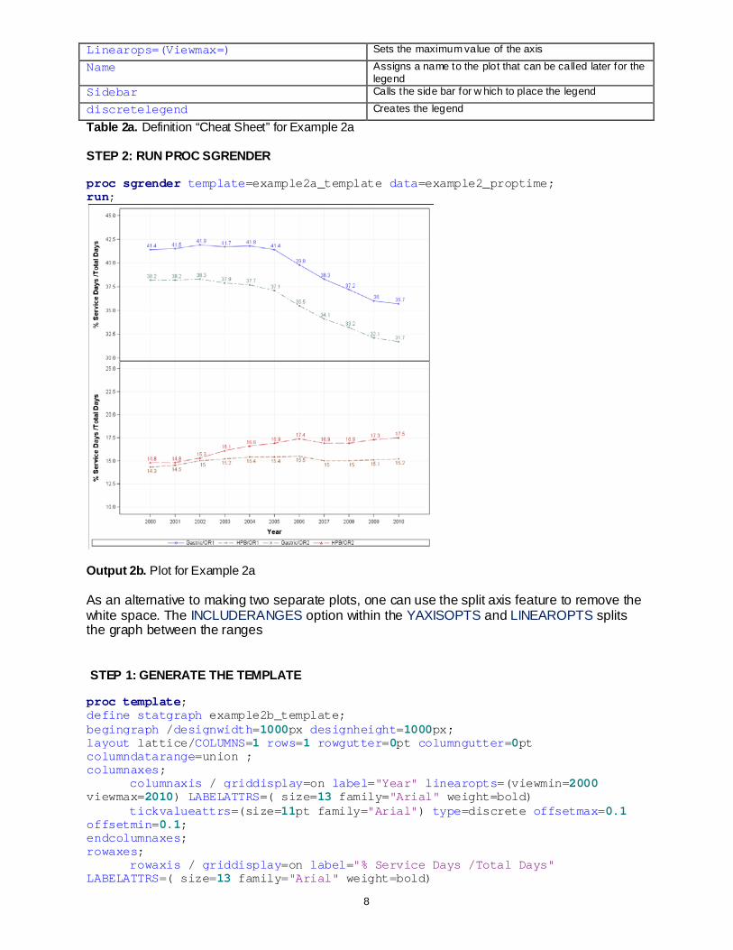
Table 2a. Definition “Cheat Sheet” for Example 2a STEP 2: RUN PROC SGRENDER proc sgrender template=example2a_template data=example2_proptime; run;

Output 2b. Plot for Example 2a As an alternative to making two separate plots, one can use the split axis feature to remove the white space. The INCLUDERANGES option within the YAXISOPTS and LINEAROPTS splits the graph between the ranges STEP 1: GENERATE THE TEMPLATE proc template; define statgraph example2b_template; begingraph /designwidth=1000px designheight=1000px; layout lattice/COLUMNS=1 rows=1 rowgutter=0pt columngutter=0pt columndatarange=union ; columnaxes; columnaxis / griddisplay=on label="Year" linearopts=(viewmin=2000 viewmax=2010) LABELATTRS=( size=13 family="Arial" weight=bold) tickvalueattrs=(size=11pt family="Arial") type=discrete offsetmax=0.1 offsetmin=0.1; endcolumnaxes; rowaxes; rowaxis / griddisplay=on label="% Service Days /Total Days" LABELATTRS=( size=13 family="Arial" weight=bold)

9

tickvalueattrs=(size=11pt family="Arial"); endrowaxes; cell ; layout overlay / yaxisopts=(display=all label="% Service Days /Total Days" griddisplay=auto_on tickvalueattrs=(size=11pt family="Arial") linearopts=(includeranges=(10-20 30-45)) LABELATTRS=( size=13 family="Arial" weight=bold)); seriesplot x=year y=eval(ifn(days_type in (2,4,5),days_prop,.)) / group=days_label datalabel=days_prop datalabelattrs=(size=11) datalabelposition=top display=all name="r" yaxis=y ; seriesplot x=year y=eval(ifn(days_type in (3),days_prop,.)) / group=days_label datalabel=days_prop datalabelattrs=(size=11) datalabelposition=bottom display=all name="r" yaxis=y ; endlayout; endcell; sidebar /align=bottom; discretelegend "r"/ border=true valueattrs=(size=11pt); endsidebar; endlayout; endgraph; end; run; quit; SAS Syntax Meaning Includeranges=() Sets the ranges to include in the axis and splits w here

the ranges do not overlap Table 2b. Definition “Cheat Sheet” for Example 2b STEP 2: RUN PROC SGRENDER proc sgrender template=example2b_template data=example2_proptime; run;

Output 2c. Plot for Example 2b

10

EXAMPLE3: WATERFALL PLOTS USING NEEDLEPLOT AND PANELING WITH WEIGHTS

In example two, we dealt with solutions for handling excessive white space within a series plot with multiple groups. This can be applied in most single figure settings including scatter plots and step plots. However, white space can occur in multiple panel plots as well. PROC SGPANEL is limited both in the plot types available and the ability to alter each figure. In this example, we’ll use PROC TEMPLATE to create waterfall plot, fix the white space, and make each plot size approximately proportional to the number of patients in the group. For this example, we’ll use data on the response to treatment based on different doses of a drug for 30 patients. The cut off for responders was a 75% reduction in tumor size. Initially, the investigator wanted a waterfall plot with each group in a separate figure. I used SGPANEL to create the figure.

proc format; value groupf 1="100mg" 2="200mg" 3="300mg" 4="400mg" 5="500mg" 6="600mg"; value responsef 0="<75% decrease" 1=">75% decrease"; run; proc sgpanel data=example5_waterfall; panelby group /rows=1 columns=6 uniscale=all NOVARNAME; label group = "Dose"; refline -75 / axis = y lineattrs=(pattern=shortdash) label=" "; vbar position / response =percent_change group=response barwidth=1; colaxis label = "Individual Patients" fitpolicy=thin; rowaxis values=(-100 to 0 by 20) label = "Change from Baseline (%)"; format group groupf. response responsef. ; run;

Output 3a. Initial Figure

The investigator liked the figure, but was concerned by the amount of white space. I thought the solution would be easy; I would use PROC TEMPLATE and create the figure using bar charts.

Similar to example 1, I used a macro to implement each of the bar charts:

11

%macro barchart(cellheader_label=,min=,max=,dose=); cell ; cellheader; entry &cellheader_label /textattrs=(size=12 family="Arial") ; endcellheader; layout overlay / yaxisopts=(display=all griddisplay=auto_on label=" " labelfitpolicy=split tickvalueattrs=(size=11pt family="Arial") linearopts=(viewmin=-100 viewmax=0) ) xaxisopts= ( label=" " discreteopts=(tickvaluefitpolicy=ROTATEALWAYS) GRIDATTRS=(thickness=10) labelfitpolicy=split tickvalueattrs=(size=11pt family="Arial") linearopts=(viewmin=&min viewmax=&max) ) border=true borderattrs=(thickness=1); barchartparm x=eval(ifn(group=&group,position,.)) y=eval(ifn(group=&group,percent_change,.)) / orient=vertical group=response; referenceline y=-75; endlayout; endcell; %mend barchart; proc template; define statgraph example3_template_v1 ; begingraph /designwidth=1000px designheight=1000px; layout lattice/COLUMNS=6 rows=1 rowgutter=0pt columngutter=0pt rowdatarange=union; rowaxes; rowaxis / griddisplay=on label="Change from Baseline (%)"; endrowaxes; %barchart(cellheader_label="100mg",min=1,max=3,group=1); %barchart(cellheader_label="200mg",min=1,max=4,group=2); %barchart(cellheader_label="300mg",min=1,max=5,group=3); %barchart(cellheader_label="400mg",min=1,max=11,group=4); %barchart(cellheader_label="500mg",min=1,max=3,group=5); %barchart(cellheader_label="600mg",min=1,max=4,group=6); endlayout; endgraph; end; run; quit;

Note: This can also be done in SGPANEL by using a non-union axis

12

Output 3b. BARCHART Figure using PROC TEMPLATE The investigator wanted all the bars to be even and I agreed as each bar represents a patient, so it shouldn’t appear that some patients have more weight than others. In both SGPANEL and in PROC TEMPLATE with BARCHART, the bar width is decided as a ratio of the maximum possible width of the plot (page 153)3. At first, I was at a loss, convinced there was no way to make the bars the same size. I searched for days, but I could not find a way to do this with BARCHART or BARCHARTPARM. I decided to look into any other possible graph formats and examined all of SAS’s examples. Luckily, I stumbled upon the example for NEEDLEPLOT, which illustrated a waterfall plot for stocks trends over time4. If one increases the size of the bars, the figure emulates a bar chart. Below is the code for how to increase the size of the bars. STEP 1: CREATE NEEDLEPLOT MACRO %macro needleplot(cellheader_label=,min=,max=,group=); cell; cellheader; entry &cellheader_label /textattrs=(size=12 family="Arial" weight=bold) ; endcellheader; layout overlay / xaxisopts= ( label=" " discreteopts=(tickvaluefitpolicy=ROTATEALWAYS) GRIDATTRS=(thickness=10) labelfitpolicy=split tickvalueattrs=(size=11pt family="Arial") linearopts=(viewmin=&min viewmax=&max TICKVALUESEQUENCE=(start=&min end=&max increment=1) ) ) border=true borderattrs=(thickness=1); needleplot x=eval(ifn(group=&group,position,.)) y=eval(ifn(group=&group,percent_change,.)) / baselineintercept=0 lineattrs=(thickness=8pt) group=response yaxis=y name="Response"; referenceline y=-90 /lineattrs=(pattern=DASH) name="r" legendlabel=" " ; endlayout; endcell; %mend needleplot; STEP 2: CREATE TEMPLATE AND IMPLEMENT MACRO proc template; define statgraph example3_template_v2; begingraph /designwidth=1000px designheight=1000px; legenditem type=text name="r2" /textattrs=(size=12pt) LABELATTRS=(size=12pt) text="75% Decrease in Tumor" ; layout lattice/COLUMNS=6 rows=1 rowgutter=0pt columngutter=0pt rowdatarange=union ; rowaxes; rowaxis / griddisplay=on label="Change from Baseline (%)" linearopts=(viewmin=-100 viewmax=0) LABELATTRS=( size=13 family="Arial" weight=bold) tickvalueattrs=(size=11pt family="Arial"); endRowaxes; %needleplot(cellheader_label="200mg",min=1,max=3,group=1); %needleplot(cellheader_label="400mg",min=1,max=4,group=2); %needleplot(cellheader_label="300mg",min=1,max=5,group=3); %needleplot(cellheader_label="600mg",min=1,max=11,group=4); %needleplot(cellheader_label="400mg",min=1,max=3,group=5); %needleplot(cellheader_label="800mg",min=1,max=4,group=6); sidebar /align=bottom; entry "Individual Patient" /textATTRS=( size=13 family="Arial" weight=bold); endsidebar;

13

sidebar / align=bottom; discretelegend "Response" / border=false valueattrs=(size=10pt); endsidebar; sidebar /align=bottom; discretelegend "r" "r2" / border=true ; endsidebar; endlayout; endgraph; end; run; quit; STEP 3: RUN PROC SGRENDER ods html style=htmlblue; proc sgrender data=example3_waterfall template = example3_template_v2; format group groupf. response responsef.; run; SAS Syntax Meaning Lineattrs=(thickness=)) Sets the thickness of the needles Legenditem Adds item to the legend using the name provided in the

plot statement. Allows one to label a reference line Baselineintercept Sets the value for w hich to sw itch direction of the

needles. Here it is set to 0 Table 3a. Definition “Cheat Sheet” for Example 3

Output 3c. Initial NEEDLEPLOT Figure using PROC TEMPLATE

As illustrated above, NEEDPLOT allows the bars can be all the same width. This resolve the initial problem of the bar width, but now, the investigator wanted the size of the plot areas to be proportional to the number of patients within each group. Fortunately, PROC TEMPLATE had a solution. Within LAYOUT LATTICE, one can use COLUMNWEIGHTS to change the size of the plots. The code and results are as follows:

STEP 1: COMPILE NEEDPLOT MACRO ABOVE STEP 2: CALCULATE THE APPROXIMATE RELATIVE WEIGHT OF THE NUMBER OF PATIENTS IN EACH PANEL RELATIVE TO THE TOTAL.

• 3/30 = 10%, • 4/30 ~ 13%,

14

• 5/30 ~ 17%, • 11/30~ 37%

Note: proc template; define statgraph example3_template_v3; begingraph /designwidth=1000px designheight=1000px; legenditem type=text name="r2" /textattrs=(size=12pt) LABELATTRS=(size=12pt) text="75% Decrease in Tumor Size" ; layout lattice/COLUMNS=6 rows=1 rowgutter=0pt columngutter=0pt /* Note: These weights are modified slightly from the initial proportions based on the appearance of the graph */ /* I recommend playing around with the weights to perfect the appearance */ columnweights=(.11 .13 .16 .36 .11 .13) rowdatarange=union border=true borderattrs=(thickness=1 color=black); rowaxes; rowaxis / griddisplay=on label="Change from Baseline (%)" linearopts=(viewmin=-100 viewmax=0) LABELATTRS=( size=13 family="Arial" weight=bold) tickvalueattrs=(size=11pt family="Arial"); endRowaxes; %needleplot(cellheader_label="200mg",min=1,max=3,group=1); %needleplot(cellheader_label="400mg",min=1,max=4,group=2); %needleplot(cellheader_label="300mg",min=1,max=5,group=3); %needleplot(cellheader_label="600mg",min=1,max=11,group=4); %needleplot(cellheader_label="400mg",min=1,max=3,group=5); %needleplot(cellheader_label="800mg",min=1,max=4,group=6); sidebar /align=bottom; entry "Individual Patient" /textATTRS=( size=13 family="Arial" weight=bold); endsidebar; sidebar / align=bottom; discretelegend "Response" / border=false valueattrs=(size=10pt); endsidebar; sidebar /align=bottom; discretelegend "r" "r2" / border=true ; endsidebar; endlayout; endgraph; end; run; quit; SAS Syntax Meaning columnweights=() Sets the w eights for each panel Table 3b. Definition “Cheat Sheet” for Example 3 Note: I modified the actual weights slightly based on the appearance of the graph. I recommend playing around with the raw numbers to improve appearance STEP 4: RUN PROC SGRENDER proc sgrender data=example3_waterfall template = example3_template_v3; format group groupf. response responsef.; run;

15

Output 3d. Final NEEDLEPLOT Figure with Panel Weights using PROC TEMPLATE

EXAMPLE 4: KAPLAN MEIER PLOT ANNOTATION

SAS includes Kaplan Meier plots within PROC LIFETEST, which is extremely useful when one needs a simple plot, and it even allows one to include number at risk. However, modifying the plot, combining with additional plots, and annotating the plot are not possible within the procedure. For instance, one wants to put overall survival (OS) and progression free survival (PFS) on one panel and then include the number at risk and estimates of median survival, one will need to use something more powerful. Fortunately, PROC TEMPLATE has a way to include all of these features in one figure. Coding these features takes a few more steps than the examples above, but can easily be replicated for other datasets.

The dataset for this example is too large to include below, so I’ve provided 10 sample lines of code to give the reader a sense of what their initial data should look like:

STEP 1: RUN PROC LIFETEST AND OUTPUT THE NECESSARY DATA ods graphics on; ods output survivalplot=sp_death_v1 CensoredSummary=cs_death_v1 Quartiles=quart_death_v1 ; proc lifetest data=example4_survival plots=s(atrisk(atrisktickonly maxlen=15) =(0 to 15 by 1)) method=km TIMELIST=(0 1 2 3 4 5 6 7 8 9 10 11 12 13 14 15) ; time death_time*death(0); label death_time= "Years from Initial Surgery"; run; ods output survivalplot=sp_pfs_v1 CensoredSummary=cs_pfs_v1 Quartiles=quart_pfs_v1 ; proc lifetest data=example4_survival plots=s(atrisk(atrisktickonly maxlen=15) =(0 to 15 by 1)) method=km TIMELIST=(0 1 2 3 4 5 6 7 8 9 10 11 12 13 14 15) ; time pfs_time*pfs(0); label pfs_time= "Years from Initial Surgery"; run; This will output three different datasets for OS and PFS

1. Survivalplot: Data points used to make the Kaplan Meier plot.

16

Obs STRATUM Time Survival AtRisk Event Censored tAtRisk StratumNum

1 1 0.0000 1.00000 180 0 . . 1

2 1 0.0000 . 180 . . 0 1

3 1 0.2053 0.99444 180 1 . . 1

4 1 0.2218 0.98889 179 1 . . 1

5 1 0.3012 0.98333 178 1 . . 1

Table 4a. Survival plot output N=10

2. CensoredSummary: The total number patients, events and patients censored

Obs Total Failed Censored PctCens

1 180 84 96 53.33

Table 4b. Censored Summary Output

3. Quartiles: Kaplan Meier Estimates of the 25th, 50th (i.e. Median), and 75th percentiles of survival along with confidence intervals

Obs STRATUM Percent Estimate Transform LowerLimit UpperLimit

1 1 75 16.2949 LOGLOG 13.7212 18.7815

2 1 50 8.2091 LOGLOG 4.9019 11.1311

3 1 25 2.5525 LOGLOG 2.1868 3.2197

Table 4c. Quartile Kaplan Meier Estimate Output STEP 2: PREPARE THE QUARTILES DATA FOR ANNOTATION AND MERGE WITH THE CENSORED SUMMARY data death_quart_v2; set death_quart_v1; /*keeps only the median estimate*/ where percent=50; /*rounds the estimate for cleaner output*/ median_est = round(estimate,0.01); /*rounds the confidence intervals and combines into one variable. Useful for cleaner output*/ /*if there is no upper confidence limit, the expression says "NR" instead for "Not Reached"*/ if upperlimit ne . then median_ci = "(" || trim(left(round(lowerlimit,0.01))) || "-" || trim(left(round(upperlimit,0.01))) || ")"; else median_ci = "(" || trim(left(round(lowerlimit,0.1))) || "- NR)"; keep median_est median_ci; run; /*merges the censored summary and quartile data for later annotation*/ data death_cs_quart_merge; merge death_cs_v1 death_quart_v2; run; Repeat Step for PFS found in Appendix STEP 3: PREPARE THE SURVIVAL DATASET FOR MERGING AND MERGE Note: It is not necessary to rename both datasets, but I find it easier for keeping track. /*rename the variables in the survival plot set for later merging*/

17

data death_sp_v2; set death_sp_v1; rename stratum = stratum_death; rename time = time_death; rename survival = survival_death; rename atrisk = atrisk_death; rename event = event_death; rename censored = censored_death; rename tatrisk = tatrisk_death; rename stratumnum = stratumnum_death; run; Repeat Step for PFS found in Appendix /*merge the two survival plot datasets*/ data survival_combined; merge sp_death_v2 pfs_sp_v2; run; STEP 4: CREATE THE ANNOTATION DATASETS AND APPEND PFS ONTO OS Many SAS users have written about the annotation procedure, so I won’t go into too much detail here. Please see the following paper for introduction to the annotation procedure5. data anno_survival; length textweight $ 6 id $ 10; length label $ 18; set death_cs_quart_merge; retain y1space "graphpercent" x1space "wallpercent" function "text" textcolor "black" textweight "normal" justify "left" TEXTSIZE 10 WIDTH 15; /*OS headers*/ x1=5; label="Subjects"; id="death_id"; y1=7; output; x1=25; label="Events"; id="death_id"; y1=7; output; x1=45; label="Censored"; id="death_id"; y1=7; output; x1=65; label="Med OS"; id="death_id"; y1=7; output; x1=80; label="(95% CI)"; id="death_id"; y1=7; output; /*OS Data*/ x1=5; label=put(total,4.0); id="death_id"; y1=3; output; x1=25; label=put(failed,4.0); id="death_id"; y1=3; output; x1=45; label=put(censored,4.0); id="death_id"; y1=3; output; x1=65; label=put(median_est,4.1); id="death_id"; y1=3; output; x1=80; label=median_ci; id="death_id"; y1=3; output; run; data anno_pfs; length textweight $ 6 id $ 10; length label $ 18; set pfs_cs_quart_merge; retain y1space "graphpercent" x1space "wallpercent" function "text" textcolor "black" textweight "normal" justify "left" TEXTSIZE 10 WIDTH 15; /*PFS headers*/ x1=5; label="Subjects"; id="pfs_id"; y1=7; output; x1=25; label="Events"; id="pfs_id"; y1=7; output; x1=45; label="Censored"; id="pfs_id"; y1=7; output; x1=65; label="Med PFS"; id="pfs_id"; y1=7; output; x1=80; label="(95% CI)"; id="pfs_id"; y1=7; output; /*PFS Data*/ x1=5; label=put(total,4.0); id="pfs_id"; y1=3; output; x1=25; label=put(failed,4.0); id="pfs_id"; y1=3; output; x1=45; label=put(censored,4.0); id="pfs_id"; y1=3; output; x1=65; label=put(median_est,4.1); id="pfs_id"; y1=3; output; x1=80; label=median_ci; id="pfs_id"; y1=3; output; run; proc append base=anno_survival data=anno_pfs force nowarn; run; SAS Syntax Meaning

18

Y1space Sets the region by w hich the annotation is placed relative to the y-axis. Graphpercent means the number is in relation to the full graph space

X1space Sets the region by w hich the annotation is laced relative to the x-axis. Wallpercent means placing the data relative to the w alls of the graph

Function Tells SAS the function of this annotation is to w rite text textcolor Font color textweight Font Weight

Justify Right, Left, or Center Justify

Textsize Font Size

Width Sets the w idth of each text space

X1 Sets the posit ion of the text relative to X1space

Y1 Sets the posit ion of the text relative to Y1space

Id Identif ies w hich annotation set this belongs to for later use in PROC TEMPLA TE

Label Actual text to be placed in the graph

Table 4d. Definition “Cheat Sheet” for Annotation in Example 4 STEP 5: CREATE AND COMPILE THE MACRO %macro km_plot (cellheader_label=,stratum=,time=,survival=,atrisk=,event=,censored=,tatrisk=,stratumnum=,annotate_id=); cell; cellheader; entry &cellheader_label /textattrs=(weight=bold size=12pt); endcellheader; layout overlay/xaxisopts=(linearopts=(viewmax=15 tickvaluelist=(0 1 2 3 4 5 6 7 8 9 10 11 12 13 14 15)) LABELATTRS=(weight=bold size=12) label="Years from Initial Surgery") yaxisopts=(label="Survival Probability" LABELATTRS=(weight=bold size=12) linearopts=(viewmin=0 viewmax=1.1 tickvaluelist=(0 0.20 0.40 0.60 0.80 1.00))); stepplot x=&time y=&survival / name="Survival" legendlabel="Survival" lineattrs=(thickness=3 ); scatterplot x=&time y=&censored / markerattrs=(symbol=plus color=black size=13) name="Censored" LEGENDLABEL="Censored"; discretelegend "Censored" / location=inside autoalign=(topright bottomleft); annotate / id=&annotate_id; innermargin / align=bottom; axistable x=&tatrisk value=&atrisk /display=(label) valueattrs=(size=10pt) ; endinnermargin; endlayout; endcell; %mend km_plot; SAS Syntax Meaning Stepplot Makes a step plot w ith time on the x-axis and survival

probability on the y-axis Scatterplot Places the censored observations at a time on the x-axis

and a spec if ied probability on the y axis annotate Tells SAS to annotate this graph Annotate / id= Identif ies w hich observations to use from the annotation

dataset Innermargin /endinnermargin Inserts inner plot margin

Axistable x= value= Puts a table relative to the x axis at time tatr isk and puts

19

the value from atrisk in Table 4e. Definition “Cheat Sheet” for Example 4 Macro STEP 6: IMPLEMENT MACRO WITHIN THE TEMPLATE proc template; define statgraph lattice_KM; begingraph /designwidth=1000px designheight=1000px; layout lattice /COLUMNS=2 rows=1 pad=(bottom=70); %km_plot(cellheader_label="Overall Survival",stratum=stratum_death,time=time_death,survival=survival_death,atrisk=atrisk_death,event=event_death, censored=censored_death, tatrisk=tatrisk_death,stratumnum=stratumnum_death,annotate_id="death_id"); %km_plot(cellheader_label="Progression Free Survival",stratum=stratum_pfs,time=time_pfs,survival=survival_pfs,atrisk=atrisk_pfs,event=event_pfs, censored=censored_pfs, tatrisk=tatrisk_pfs,stratumnum=stratumnum_pfs,annotate_id="pfs_id"); endlayout; endgraph; end; run; quit; SAS Syntax Meaning Pad Adds a padding betw een the end of the cell and the

graph w here the annotation w ill go. Bottom tells SAS to do this at the bottom of the plot

Table 4f. Definition “Cheat Sheet” for Example 4 Template STEP 6: RUN PROC SGRENDER ods graphics on /width=10in height=8in; proc sgrender data=survival_combined sganno=anno_survival template=lattice_KM; run;

Output 4a. Combined Kaplan Meier Plot with Number and Risk and Survival Estimates Note: Please feel free to contact me for code on how to implement this with multiple strata

20

CONCLUSIONS

PROC TEMPLATE expands the graphical capabilities of SGPLOT and SGPANEL, allowing one to do an incredible amount of modifications. This paper demonstrated how to create a panel plot for different variables, a split plot using select observations, a broken axis plot for select observations, and a waterfall plot using NEEDLEPLOT. Additionally, we demonstrated how to weight each panel in a plot and how to combine and annotate Kaplan Meier plots. These are just a few of the opportunities available to users of PROC TEMPLATE that eliminate the need for post output processing or use of other statistical software. Familiarizing oneself with PROC TEMPLATE is one step on the road to complete automation with SAS. REFERENCES

1. Pratt, Jesse M. 2012. “The Graph Template Language: Beyond the SAS/GRA PH Procedures”. PSAS Global Forum Paper 285-2012. Available at: http://support.sas.com/resources/papers/proceedings12/285-2012.pdf

2. SAS Institute Inc. 2012. SAS® 9.3 Graph Template Language: Reference, Third Edit ion. Cary, NC: SAS Institute Inc

3. SAS Institute Inc. 2010. SAS® 9.2 Graph Template Language: Reference, Third Edit ion. Cary, NC: SAS Institute Inc

4. SAS Institute Inc. 2010. “Example Program and Statement Details: Available at: http://support.sas.com/documentation/cdl/en/grstatgraph/63878/HTML/default/view er.htm#p0dc ix1s0khu6fn1qj4tudw sy72a.htm

5. Mantange, S. 2014. “Annotate your SGPLOT Graphs”. Paper CC01-2014. Available at: http://www.pharmasug.org/proceedings/china2014/CC/PharmaSUG-China-2014-CC01.pdf

ACKNOWLEDGEMENTS All datasets presented here are s imulated versions of datasets and research study objectives w ere modif ied. No actual patient data or true research study objectives w ere used for the purpose of this presentation. I w ould like to thank Esther Drill for review ing the overall concepts presented in this paper. CONTACT INFORMATION Your comments and questions are valued and encouraged. Contact the author at: Debra A. Goldman Memor ial Sloan Kettering Cancer Center 484 Lex ington Avenue 2nd Floor New York, NY 10022 646-888-8331 goldmand@mskcc.org https://www.mskcc.org/profile/debra-goldman SAS and all other SAS Institute Inc. product or service names are registered trademarks or trademarks of SAS Institute Inc. in the USA and other countries. ® indicates USA registration.

Other brand and product names are trademarks of their respective companies.

21

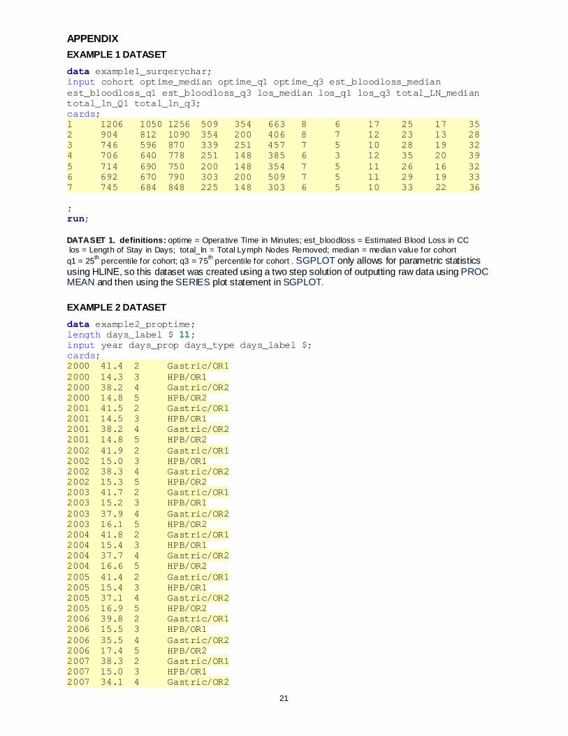
APPENDIX EXAMPLE 1 DATASET data example1_surgerychar; input cohort optime_median optime_q1 optime_q3 est_bloodloss_median est_bloodloss_q1 est_bloodloss_q3 los_median los_q1 los_q3 total_LN_median total_ln_Q1 total_ln_q3; cards; 1 1206 1050 1256 509 354 663 8 6 17 25 17 35 2 904 812 1090 354 200 406 8 7 12 23 13 28 3 746 596 870 339 251 457 7 5 10 28 19 32 4 706 640 778 251 148 385 6 3 12 35 20 39 5 714 690 750 200 148 354 7 5 11 26 16 32 6 692 670 790 303 200 509 7 5 11 29 19 33 7 745 684 848 225 148 303 6 5 10 33 22 36 ; run; DATASET 1. definitions: optime = Operative Time in Minutes; est_bloodloss = Estimated Blood Loss in CC los = Length of Stay in Days; total_ln = Total Lymph Nodes Removed; median = median value for cohort q1 = 25th percentile for cohort; q3 = 75th percentile for cohort . SGPLOT only allows for parametric statistics using HLINE, so this dataset was created using a two step solution of outputting raw data using PROC MEAN and then using the SERIES plot statement in SGPLOT.

EXAMPLE 2 DATASET data example2_proptime; length days_label $ 11; input year days_prop days_type days_label $; cards; 2000 41.4 2 Gastric/OR1 2000 14.3 3 HPB/OR1 2000 38.2 4 Gastric/OR2 2000 14.8 5 HPB/OR2 2001 41.5 2 Gastric/OR1 2001 14.5 3 HPB/OR1 2001 38.2 4 Gastric/OR2 2001 14.8 5 HPB/OR2 2002 41.9 2 Gastric/OR1 2002 15.0 3 HPB/OR1 2002 38.3 4 Gastric/OR2 2002 15.3 5 HPB/OR2 2003 41.7 2 Gastric/OR1 2003 15.2 3 HPB/OR1 2003 37.9 4 Gastric/OR2 2003 16.1 5 HPB/OR2 2004 41.8 2 Gastric/OR1 2004 15.4 3 HPB/OR1 2004 37.7 4 Gastric/OR2 2004 16.6 5 HPB/OR2 2005 41.4 2 Gastric/OR1 2005 15.4 3 HPB/OR1 2005 37.1 4 Gastric/OR2 2005 16.9 5 HPB/OR2 2006 39.8 2 Gastric/OR1 2006 15.5 3 HPB/OR1 2006 35.5 4 Gastric/OR2 2006 17.4 5 HPB/OR2 2007 38.3 2 Gastric/OR1 2007 15.0 3 HPB/OR1 2007 34.1 4 Gastric/OR2

22

2007 16.9 5 HPB/OR2 2008 37.2 2 Gastric/OR1 2008 15.0 3 HPB/OR1 2008 33.2 4 Gastric/OR2 2008 16.9 5 HPB/OR2 2009 36.0 2 Gastric/OR1 2009 15.1 3 HPB/OR1 2009 32.1 4 Gastric/OR2 2009 17.3 5 HPB/OR2 2010 35.7 2 Gastric/OR1 2010 15.2 3 HPB/OR1 2010 31.7 4 Gastric/OR2 2010 17.5 5 HPB/OR2 ; run; DATASET 2. definitions: year= year; days_prop = proportion of dats, days_type = numeric grouping of the cohort in which the proportion belongs to; days_label = categorical grouping of the cohort in w hich the proportion belongs to EXAMPLE 3 DATASET data example3_waterfall; input ID group percent_change position response; datalines; 1 1 -85 1 1 2 1 -67 2 0 3 1 -60 3 0 4 2 -92 1 1 5 2 -50 2 0 6 2 -48 3 0 7 2 -23 4 0 8 3 -99 1 1 9 3 -97 2 1 10 3 -77 3 1 11 3 -20 4 0 12 3 -14 5 0 13 4 -100 1 1 14 4 -100 2 1 15 4 -94 3 1 16 4 -93 4 1 17 4 -92 5 1 18 4 -87 6 1 19 4 -77 7 1 20 4 -77 8 1 21 4 -70 9 0 22 4 -50 10 0 23 4 -39 11 0 24 5 -100 1 1 25 5 -94 2 1 26 5 -92 3 1 27 6 -100 1 1 28 6 -100 2 1 29 6 -98 3 1 30 6 -76 4 1 ; run;

DATASET 3. definitions: id = patient identif ier; group = drug grouping patient belongs to; percent_change = percent change in tumor size from baseline to follow up imaging; posit ion = w ithin group posit ion in the plot; response = dichotomous variable indicating w hether percent change w as greater than or less than 75%

EXAMPLE 4 DATASET data example4_survival;

23

input id death_time death pfs_time pfs; datalines; 1 0.3451 1 0.1214 1 2 14.3858 0 14.1784 0 3 0.493 1 0.1762 1 4 0.4163 1 0.1104 1 5 0.7341 0 0.7256 0 6 0.7194 1 0.1159 1 7 10.0937 1 9.3652 1 8 12.0197 0 11.8146 0 9 18.5701 1 18.5701 1 10 13.5118 1 13.5118 1

………. ; run;

DATASET 4. definitions: id= patient id; death_time = time from surgery until death or last follow up if censored; death=event indicator w here 1 means dead and 0 means censored; pfs_time= time from surgery until progression, death or last follow up if censored; pfs= event indicator w here 1 means progression or death and 0 means censored.

EXAMPLE 4 REPEAT STEP FOR PFS data pfs_quart_v2; set pfs_quart_v1; /*keeps only the median estimate*/ where percent=50; /*rounds the estimate for cleaner output*/ median_est = round(estimate,0.01); /*rounds the confidence intervals and combines into one variable. Useful for cleaner output*/ /*if there is no upper confidence limit, the expression says "NR" instead for "Not Reached"*/ if upperlimit ne . then median_ci = "(" || trim(left(round(lowerlimit,0.01))) || "-" || trim(left(round(upperlimit,0.01))) || ")"; else median_ci = "(" || trim(left(round(lowerlimit,0.1))) || "- NR)"; keep median_est median_ci; run; /*merges the censored summary and quartile data for later annotation*/ data pfs_cs_quart_merge; merge pfs_cs_v1 pfs_quart_v2; run;

data pfs_quart_v2; set pfs_quart_v1; /*keeps only the median estimate*/ where percent=50; /*rounds the estimate for cleaner output*/ median_est = round(estimate,0.01); /*rounds the confidence intervals and combines into one variable. Useful for cleaner output*/ /*if there is no upper confidence limit, the expression says "NR" instead for "Not Reached"*/ if upperlimit ne . then median_ci = "(" || trim(left(round(lowerlimit,0.01))) || "-" || trim(left(round(upperlimit,0.01))) || ")"; else median_ci = "(" || trim(left(round(lowerlimit,0.1))) || "- NR)"; keep median_est median_ci; run; /*merges the censored summary and quartile data for later annotation*/ data pfs_cs_quart_merge; merge pfs_cs_v1 pfs_quart_v2; run;