Bounding Betti Numbers of Sets

Definable in O-Minimal

Structures Over the Realssubmitted by

Mahana Cluthafor the degree of Doctor of Philosophy

of the

University of BathDepartment of Computer Science

January 2011

COPYRIGHT

Attention is drawn to the fact that copyright of this thesis rests with its author. This copy

of the thesis has been supplied on the condition that anyone who consults it is understood to

recognise that its copyright rests with its author and that no quotation from the thesis and no

information derived from it may be published without the prior written consent of the author.

This thesis may be made available for consultation within the University Library and may be

photocopied or lent to other libraries for the purposes of consultation.

Signature of Author . . . . . . . . . . . . . . . . . . . . . . . . . . . . . . . . . . . . . . . . . . . . . . . . . . . . . . . . . . . . . . . . . . . . . . . . .

Mahana Clutha

1

Summary

A bound for Betti numbers of sets definable in o-minimal structures is presented.

An axiomatic complexity measure is defined, allowing various concrete complexity measures

for definable functions to be covered. This includes common concrete measures such as the

degree of polynomials, and complexity of Pfaffian functions.

A generalisation of the Thom-Milnor Bound [17, 19] for sets defined by the conjunction

of equations and non-strict inequalities is presented, in the new context of sets definable in o-

minimal structures using the axiomatic complexity measure. Next bounds are produced for sets

defined by Boolean combinations of equations and inequalities, through firstly considering sets

defined by sign conditions, then using this to produce results for closed sets, and then making

use of a construction to approximate any set defined by a Boolean combination of equations

and inequalities by a closed set.

Lastly, existing results [12] for sets defined using quantifiers on an open or closed set are

generalised, using a construction from Gabrielov and Vorobjov [11] to approximate any set by

a compact set. This results in a method to find a general bound for any set definable in an

o-minimal structure in terms of the axiomatic complexity measure. As a consequence for the

first time an upper bound for sub-Pfaffian sets defined by arbitrary formulae with quantifiers

is given. This bound is singly exponential if the number of quantifier alternations is fixed.

2

3

Acknowledgements

Thanks to Nicolai and Guy for their support and patience with an unusual student.

Thanks to the worldwide judo family for providing the perfect complement to a research

degree.

Thanks to my real family – the Cluthas, the Weirs and the Rigarlsfords.

Special thanks to Lance, Sally, Cassie and Tom for being my adoptive kiwi family so far from

home.

Also special thanks to the Cousins for being my British adoptive family.

Faith – words are inadequate to portray the value of your friendship.

For Isobel, Jane and Florence. Three generations of exceptional women.

4

5

Contents

1 Preliminaries 9

1.1 Introduction . . . . . . . . . . . . . . . . . . . . . . . . . . . . . . . . . . . . . . 9

1.2 Previous Work . . . . . . . . . . . . . . . . . . . . . . . . . . . . . . . . . . . . 9

1.3 Outline . . . . . . . . . . . . . . . . . . . . . . . . . . . . . . . . . . . . . . . . 10

1.4 Main Results . . . . . . . . . . . . . . . . . . . . . . . . . . . . . . . . . . . . . 11

1.5 Background . . . . . . . . . . . . . . . . . . . . . . . . . . . . . . . . . . . . . . 12

1.5.1 O-Minimal Structures . . . . . . . . . . . . . . . . . . . . . . . . . . . . 12

1.5.2 Pfaffian Functions . . . . . . . . . . . . . . . . . . . . . . . . . . . . . . 13

1.5.3 Hardt’s Triviality . . . . . . . . . . . . . . . . . . . . . . . . . . . . . . . 14

1.5.4 Complexity Notation . . . . . . . . . . . . . . . . . . . . . . . . . . . . . 15

1.5.5 Sard’s Theorem . . . . . . . . . . . . . . . . . . . . . . . . . . . . . . . . 15

1.5.6 Basic concepts in Algebraic Topology . . . . . . . . . . . . . . . . . . . 16

1.5.7 Significantly Small Real Numbers . . . . . . . . . . . . . . . . . . . . . . 16

1.5.8 Mayer-Vietoris Inequalities . . . . . . . . . . . . . . . . . . . . . . . . . 16

1.6 Complexity . . . . . . . . . . . . . . . . . . . . . . . . . . . . . . . . . . . . . . 17

1.6.1 The Functions κ and γ . . . . . . . . . . . . . . . . . . . . . . . . . . . . 20

2 Sets defined by equalities and non-strict inequalities 21

2.1 Sets defined by equalities . . . . . . . . . . . . . . . . . . . . . . . . . . . . . . 21

2.1.1 Introduction . . . . . . . . . . . . . . . . . . . . . . . . . . . . . . . . . 21

2.1.2 Main Result . . . . . . . . . . . . . . . . . . . . . . . . . . . . . . . . . . 21

2.1.3 Projections and Morse Functions . . . . . . . . . . . . . . . . . . . . . . 22

2.1.4 A Bounding Hypersurface . . . . . . . . . . . . . . . . . . . . . . . . . . 26

2.1.5 Proof of main result . . . . . . . . . . . . . . . . . . . . . . . . . . . . . 27

2.2 Sets defined by multiple non-strict inequalities . . . . . . . . . . . . . . . . . . 29

3 Sets defined by a Boolean combination of functions 32

3.1 Preliminaries . . . . . . . . . . . . . . . . . . . . . . . . . . . . . . . . . . . . . 32

3.1.1 The Function Ω . . . . . . . . . . . . . . . . . . . . . . . . . . . . . . . . 32

3.1.2 Main Result . . . . . . . . . . . . . . . . . . . . . . . . . . . . . . . . . . 33

3.2 Realisation of Sign Conditions . . . . . . . . . . . . . . . . . . . . . . . . . . . . 33

6

3.2.1 Sign Conditions . . . . . . . . . . . . . . . . . . . . . . . . . . . . . . . . 34

3.3 Closed Sets . . . . . . . . . . . . . . . . . . . . . . . . . . . . . . . . . . . . . . 35

3.4 Arbitrary Boolean Combinations . . . . . . . . . . . . . . . . . . . . . . . . . . 39

4 Sets Defined with Quantifiers 48

4.1 Introduction . . . . . . . . . . . . . . . . . . . . . . . . . . . . . . . . . . . . . . 48

4.2 Sidenote – the case where Xν is open or closed . . . . . . . . . . . . . . . . . . 49

4.3 A Spectral Sequence Associated with a Surjective Map . . . . . . . . . . . . . . 49

4.4 Alexander’s duality . . . . . . . . . . . . . . . . . . . . . . . . . . . . . . . . . . 50

4.5 Approximation of Definable Sets by Compact Families . . . . . . . . . . . . . . 50

4.5.1 Projections . . . . . . . . . . . . . . . . . . . . . . . . . . . . . . . . . . 53

4.6 Notation . . . . . . . . . . . . . . . . . . . . . . . . . . . . . . . . . . . . . . . . 55

4.6.1 General Intersections and Unions . . . . . . . . . . . . . . . . . . . . . . 56

4.7 Application of Spectral Sequence Result . . . . . . . . . . . . . . . . . . . . . . 58

4.8 Outline of Proof . . . . . . . . . . . . . . . . . . . . . . . . . . . . . . . . . . . 59

4.9 Quantifiers . . . . . . . . . . . . . . . . . . . . . . . . . . . . . . . . . . . . . . 59

4.9.1 One Existential Quantifier . . . . . . . . . . . . . . . . . . . . . . . . . . 60

4.9.2 One Universal Quantifier . . . . . . . . . . . . . . . . . . . . . . . . . . 60

4.9.3 Two Quantifiers - . . . . . . . . . . . . . . . . . . . . . . . . . . . . 63∃ ∀

4.9.4 Three Quantifiers - ∃ ∀ ∃ . . . . . . . . . . . . . . . . . . . . . . . . . . . 65

4.9.5 Arbitrary number of Quantifiers . . . . . . . . . . . . . . . . . . . . . . 66

4.10 Upper Bounds . . . . . . . . . . . . . . . . . . . . . . . . . . . . . . . . . . . . 70

Bibliography 78

7

8

Chapter 1

Preliminaries

1.1 Introduction

This thesis considers the problem of relating the complexity of a formula to the complexity

of the “shape” it describes. The natural questions arising from this initial statement of the

problem are “what type of formula?”, “how do we measure the complexity of the formula?”

and “how do we measure the complexity of the shape?”.

There are a variety of answers to the first two questions. Existing work in this area mostly

deals with polynomial functions, with degree as complexity measure. Some work has been done

with Pfaffian functions (for example [22]), see Section 1.5.2 for definitions and the relevant

complexity measure. This thesis, however, considers a more general type of formula, that is

sets definable in o-minimal structures over the reals (see Section 1.5.1). There is not standard

method of measuring the complexity of such formula, hence one of the main contributions of

this work is to define an axiomatic complexity measure to solve this problem.

The final question has a standard answer – we measure the complexity of “shapes”, i.e.

some sort of geometric complexity, using Betti numbers. These are defined in Section 1.5.6. In

the following we frequently bound the sum of the Betti numbers of a given set, which obviously

bounds each individual Betti number (as they are a finite sequence of integers).

1.2 Previous Work

In 1964 Milnor [17] considered a real algebraic set S ⊂ Rn, defined by polynomial equations

f1(x1, . . . , xm) = . . . = fp(x1, . . . , xm) = 0

of maximum degree d. He showed the sum of the Betti numbers of S is bounded by d(2d−1)n−1 .

Milnor also showed that if the p equations above were instead non-strict inequalities, and they

have total degree d� = deg(f1) + . . . + deg(fp), then the Betti sum of the set defined by these

inequalities is bounded by 12 (2 + d�)(1 + d�)n−1 . Various alternate versions of the above results

9

have been published (see Petrovskii and Oleinik [18], Thom [19]), and modified, simpler proofs

offered (for example Basu, Pollack, Roy [2]).

In 1999 Basu [1] showed that if a closed semi-algebraic set S ⊂ Rn is defined as the inter­

section of a real algebraic set Q = 0, where Q is a polynomial with deg(Q) ≤ d, whose real

dimension is n�, with a set defined by a quantifier-free Boolean formula with no negations with

atoms of the form Pi = 0, Pi ≥ 0, Pi ≤ 0, for 1 ≤ i ≤ s, and the degree of polynomials Pi being

at most d, then the sum of the Betti numbers of S is bounded by sn� (O(d))n . In 2004 Basu,

Pollack and Roy [3] refined this bound to

n� � �� n��−i s 6j d(2d − 1)n−1 .

ji=0 j=0

In the same paper a bound is also constructed for the sum of the i-th Betti numbers over the

realisation of all sign conditions of a set of polynomials on an algebraic set.

The preceding results all concern sets defined in terms of polynomials. In 1999, Zell [22]

produced a similar result for semi-Pfaffian sets, directly following the above methods. Further

to this, a survey of upper bounds on sets defined by Pfaffian and Noetherian functions is

presented in [9].

In 2005, Gabrielov and Vorobjov [10] described a way to replace any arbitrary semi-algebraic

set, defined by a arbitrary Boolean quantifier-free formula, by a compact set with coinciding

Betti numbers, and presented a bound of O(k2d)n . In the second edition of [2] an alternative,

simpler proof of this result is given, showing homotopy equivalence rather than simply coinciding

Betti numbers.

As the Tarski-Seidenberg Theorem (see for example [7]) states that in the semi-algebraic

case, every first-order formula is equivalent to a quantifier-free formula, the polynomial case is

essentially complete, save refinements of bounds. Sets defined in o-minimal structures however,

do not generally have this property, for example see [8].

Gabrielov, Vorobjov and Zell [12] showed how to associate a spectral sequence with a surjec­

tive map, and used this to find an upper bound for open and closed sets defined by first-order

formulae. In particular, results are presented for sub-Pfaffian sets defined by first-order formu­

lae. This is one of the main ingredients of the last chapter of this thesis, and indeed one of the

primary aims of this work is to remove the restriction that requires sets to be open or closed.

In 2009, Gabrielov and Vorobjov [11] presented a method for approximating any o-minimal

set S by a compact o-minimal set T , with each Betti number of S being bounded by that of

T , and, in a particular case, these sets are shown to be homotopy equivalent. This result leads

to a refinement of some of the above bounds in the semi-algebraic and semi- and sub- Pfaffian

cases, and, more importantly, presents a method that can be used for any o-minimal set.

1.3 Outline

Existing work suggests two areas for expansion.

10

Firstly, we seek to reproduce the above results, this time for functions defined in o-minimal

structures instead of simply polynomials or Pfaffian functions. We start with sets defined by

equalities, then closed sets, then sets defined by an arbitrary Boolean combination, before

finally considering sets defined using quantifiers.

The second new area derives naturally from this problem – established complexity measures

for polynomials (for example degree, number of monomials, additive complexity) and Pfaffian

functions exist, but there is no conventional way to measure the complexity of a function

defined in an o-minimal structure. So, before proceeding with the above calculations, we create

an axiomatic complexity definition. The definition presented in this work was inspired by [4].

The remainder of this chapter consists of definitions and results from existing work that

are used in our proofs, and concludes with a presentation of our new axiomatic complexity

definition. In Chapter 2 we start with the case of a set defined by multiple equalities, following

the methods of Milnor, then move on to sets defined by the conjunction of equations and non-

strict inequalities. Chapter 3 initially shows how to bound the Betti numbers of sign conditions,

then uses this to bound the Betti numbers of closed sets. Lastly a construction is presented

to approximate a set defined by any Boolean combination of equations and inequalities by a

closed set, and this, in conjunction with the previous result, gives a bound of the Betti numbers

of the original set. The final chapter considers sets defined using quantifiers, and is the most

significant contribution of this thesis. In [12] a method is presented to bound the Betti numbers

of a surjective map, using a particular spectral sequence, and then this is used in the case of

the projective map to bound the Betti numbers of a open or closed set defined with quantifiers.

In [11], a method is shown to approximate any set with a compact set. The main result of

this thesis combines these two results, along with the preceding work, to give a bound for any

set defined in an o-minimal structure using quantifiers. As a consequence for the first time an

upper bound for sub-Pfaffian sets defined by arbitrary formulae with quantifiers is given. This

bound is singly exponential if the number of quantifier alternations is fixed.

Our methods are necessary for sub-Pfaffian sets, as there is no equivalent to Tarski-Seidenberg

for polynomials. As is made clear in Section 1.5.2, a restricted sub-Pfaffian set need not be

semi-Pfaffian, and there is no quantifier elimination. This is therefore also true for sets definable

in o-minimal structures over the reals (as this includes sets defined by Pfaffian functions).

1.4 Main Results

This thesis has three main contributions to knowledge:

• A new axiomatic complexity metric is defined in Section 1.6, which improves on the

presentation in [4].

• Know quantitative bounds in polynomial and Pfaffian settings are generalized to our new

setting of sets definable in o-minimal structures. These new results reduce to existing

results in the polynomial and Pfaffian cases.

11

• New results are produced in the o-minimal setting for quantified formula over sets which

need not be open or closed. The application of this to the Pfaffian case is also new. Main

Result A (Theorem 4.9.8) gives a bound in terms of the summation of sets, and Main

Result B (Theorem 4.10.7, really a Corollary of Theorem 4.9.8) gives a specific bound in

terms of the complexity metric.

1.5 Background

1.5.1 O-Minimal Structures

A very good text on this subject is [20]. The following two definitions are taken directly from

[6]:

Definition 1.5.1. A structure expanding the real closed field R is a collection S = (Sn)n∈N,

where each Sn is a set of subsets of the affine space Rn, satisfying the following axioms:

1. All algebraic subsets of Rn are in Sn

2. For every n, Sn is a Boolean subalgebra of the powerset of Rn

3. If A ∈ Sm, and B ∈ Sn, then A × B ∈ Sm+n

4. If p : Rn+1 → Rn is the projection on the first n coordinates, and A ∈ Sn+1, then

p(A) ∈ Sn.

The elements of Sn are called the definable subsets of Rn . The structure S is said to be

o-minimal if, moreover, it satisfies:

5. The elements of S1 are precisely the finite unions of points and intervals.

Definition 1.5.2. A map f : A → Rp (where A ⊂ Rn) is called definable if its graph is a

definable subset of Rn × Rp.

Conic Structure

Let Bn(a, r) denote the closed ball in Rn with radius r, centered at a, and let Sn(a, r) denote

the sphere in Rn with radius r, centered at a. The following Theorems are taken from [6]

Theorem 1.5.3 (Local Conic Structure). Let A ⊂ Rn be a closed definable set, and a a point

in A. There is a r > 0 such that there exists a definable homeomorphism h from the cone with

vertex a and base Sn(a, r)∩A onto Bn(a, r)∩A satisfying h|Sn(a,r)∩A = Id and |h(x)−a| = |x−a|for all x in the cone.

The following theorem tells us that any closed definable set is homotopy equivalent to the

intersection of that set with a ball of sufficiently large radius. This is useful later when we

have a closed set defined by a combination of equations and/or inequalities, and we require a

compact set – we only need to add one additional inequality.

12

�

Theorem 1.5.4 (Conic Structure at Infinity). Let A ⊂ Rn be a closed definable set. Then there

exists r ∈ R, r > 0, such that for every r�, r� ≥ r, there is a definable deformation retraction

from A to Ar� = A ∩ Bn(0, r�) and a definable deformation retraction from Ar� to Ar.

Proof. Let us suppose A is not bounded. Through an inversion map φ : Rn \ 0 → Rn \ 0,

φ(x) = x/|x|2, we can reduce to the property of local conic structure for φ(A) ∪ 0 at 0.

This theorem can be visualised as follows: consider a simplicial complex K equivalent to A.

Take r large enough so that each simplex in K intersects with the ball of radius r, and each

bounded simplex is a subset of the ball. Then each unbounded simplex can be “shrunk” in,

and be replaced with an equivalent bounded simplex, without affecting the homotopy type.

1.5.2 Pfaffian Functions

We present a definition for Pfaffian functions from [9], modified to only include the real case:

Definition 1.5.5. A Pfaffian chain of the order r ≥ 0 and degree α ≥ 1 in an open domain

G ⊂ Rn is a sequence of analytic functions f1, . . . fr in G satisfying differential equations

dfj (x) = gij (x, f1(x), . . . , fj (x))dxi 1≤i≤n

for 1 ≤ j ≤ r. Here gij (x, y1, . . . , yj ) are polynomials in x = (x1, . . . , xn), y1, . . . , yj of degrees

not exceeding α. A function f(x) = P (x, f1(x), . . . , fj (x)), where P (x, f1(x), . . . , fj (x)) is a

polynomial of a degree not exceeding β ≥ 1, is called a Pfaffian function of order r and degree

(α, β). Note that the Pfaffian function f is defined only in the domain G where all functions

f1, . . . , fr are analytic, even if f itself can be extended as an analytic function to a larger

domain.

We present a few examples to illustrate, taken from [9].

Example 1.5.6. (a) Pfaffian functions of order 0 and degree (1, β) are polynomials of degree

not exceeding β.

(b) The exponential function f(x) = eax is a Pfaffian function of order 1 and degree (1, 1) in

R, due to the equation df(x) = af(x)dx.

(c) The function f(x) = 1/x is a Pfaffian function of order 1 and degree (2, 1) in the domain

= 0}, due to the equation df(x) = −f2(x)dx.{x ∈ R : x �

(d) The polynomial f(x) = xm can be viewed as a Pfaffian function of order 2 and degree (2, 1)

in the domain {x ∈ R : x = 0� } (but not in R), due to the equations df(x) = mf(x)g(x)dx

and dg(x) = −g2(x)dx, where g(x) = 1/x.

The expansion of R by sets defined by Pfaffian functions was proven to be o-minimal in [21].

The following lemmas and definitions are also taken from [9].

13

Lemma 1.5.7. The sum (resp. product) of two Pfaffian functions f1 and f2 of orders r1 and

r2 and degrees (α1, β1) and (α2, β2) respectively, is a Pfaffian function of order r1 + r2 and

degree (α, max{β1, β2}) (resp. (α, β1 + β2), where α = max{α1, α2}. If the two functions are

defined by the same Pfaffian chain of order r, then the orders of the sum and the product are

both equal to r.

Lemma 1.5.8. A partial derivative of a Pfaffian function of order r and degree (α, β), is a

Pfaffian function having the same Pfaffian chain of order r, and degree (α, α + β − 1).

Definition 1.5.9. A set X ⊂ Rn is called semi-Pfaffian in an open domain G ⊂ Rn if it consists

of points in G satisfying a Boolean combination F of some atomic equations and inequalities

f = 0, g > 0, where f, g are Pfaffian functions having a common Pfaffian chain defined in G.

We will write X = {F}. A semi-Pfaffian set X is restricted in G if its topological closure lies

in G. A semi-Pfaffian set is called basic if the Boolean combination is just a conjunction of

equations and strict inequalities.

Definition 1.5.10. A set X ⊂ Rn is called sub-Pfaffian in an open domain G ⊂ Rn if it is an

image of a semi-Pfaffian set under a projection into a subspace.

Definition 1.5.11. Consider the closed cube Im+n = [−1, 1]m+n in an open domain G ⊂

Rm+n, and the projection map π : Rm+n → Rn . A subset Y ⊂ In is called restricted sub-

Pfaffian if Y = π(X) for a restricted semi-Pfaffian set X ⊂ Im+n .

Note that a restricted sub-Pfaffian set need not be semi-Pfaffian, see [9] for an example.

This is the most significant difference between the theories of semi- and sub-Pfaffian sets on

the one hand, and semialgebraic sets on the other, and is a key reason this thesis is needed.

We now present an analogue of Bezout’s theorem for Pfaffian functions:

Theorem 1.5.12 (Khovanskii, [15], [16]). Consider a system of equations f1 = . . . = fn = 0,

where fi, 1 ≤ i ≤ n, are Pfaffian functions in a domain G ⊂ Rn, having a common Pfaffian

chain of order r, and degrees (α, βi) respectively. Then, the number of non-degenerate solutions

of this system does not exceed

M(n, r, α, β1, . . . , βn) = 2r(r−1)/2β1 . . . βn(min{n, r}α + β1 + . . . + βn − n + 1)r .

1.5.3 Hardt’s Triviality

The following is taken from [6].

Definition 1.5.13. Let X ⊂ Rm × Rn be a definable family, and denote by πm the projection

onto Rm . Let A be a definable subset of Rm, and let XA = X ∩(A×Rn). We say that the family

X is definably trivial over A if there exists a definable set F and a definable homeomorphism

h : A × F XA such that, for x ∈ A × F→

πm(h(x)) = πm(x).

14

�

We say that h is a definable trivialisation of X over A. Now let Y be a definable subset

of X. We say that the trivialisation h is compatible with Y if there is a definable subset G of

F such that h(A × G) = YA. Note that if h is compatible with Y , its restriction to YA is a

trivialisation of Y over A.

Theorem 1.5.14 (Hardt’s Theorem for Definable Families). Let X ⊂ Rm × Rn be a defin­

able family. Let Y1, . . . , Yl be definable subsets of X. There exists a finite partition of Rm

into definable sets C1, . . . , Ck such that X is definably trivial over each Ci, and moreover, the

trivilisations over each Ci are compatible with Y1, . . . , Yl.

This will frequently be used in a situation like the following (see Definition 2.1.5 for nota­

tion).

Example 1.5.15. For a definable set A ⊂ Rn there exists a homeomorphism φ : Aa × (0, a] →

A(0,a]. Moreover the homeomorphism can be chosen so that for x ∈ Aa, y ∈ (0, a), the projection

onto the second factor of φ(x, y) is y, and φ(Aa, a) = Aa.

1.5.4 Complexity Notation

In this thesis we use some notation that is not standard to Complexity theory. The “O” notation

that follows is as normal, but the “o” notation is defined differently (taken from [2]), and Ω is

a function defined later in the text, and is nothing to do with complexity.

We use the notation, whenever a more explicit bound is not more useful.

Definition 1.5.16. We say f(x) ≤ O(g(x)) if there exists a positive real number M and an

x0 ∈ R such that

|f(x)| ≤ M |g(x)|

for all x > x0.

The following notation allows us to express how “small” certain expressions are, and is taken

from [2]

Definition 1.5.17. For an expression f = i(aiδri ), where ai = 0 and � δ is taken to be very

small, we denote by o(f) the smallest value of ri.

1.5.5 Sard’s Theorem

The following is taken from [14]:

Definition 1.5.18. An n-cube C ⊂ Rn of edge λ > 0 is a product C = I1 × . . . × In of closed

intervals of length λ. The measure of C is λn . A subset X ⊂ Rn has measure zero if for every

ε > 0 it can be covered by a family of n-cubes, the sum of whose measures is less than ε.

Lemma 1.5.19. A countable union of sets of measure zero has measure zero.

Proof. Trivial.

15

�

Theorem 1.5.20 (Sard’s Theorem). Let M , N be manifolds of dimensions m, n and f : M →

N a Cr map. If r > max{0,m − n} then the set of critical values of f has measure zero in N .

1.5.6 Basic concepts in Algebraic Topology

For a topological space X, we denote by Hi(X) its i-th homology group, and by bi(X) =

rank Hi(X) its i-th Betti number. We denote by b(X) = i bi(X) the sum of the Betti

numbers of S.

Lemma 1.5.21. The number of connected components of a non-empty closed and bounded

definable set S is equal to b0(S)

Proof. See for example Proposition 6.26 of [2].

Since in this thesis we spend very little time dealing with homotopy groups, we usually use

the symbol π for projections. However, in the few cases where we must mention homotopy

groups, we follow the standard convention of using πi(X) to denote the i-th homotopy group

of X, but clearly explain the situation to avoid any confusion.

The symbol � denotes homotopy equivalence. If Y ⊂ X, then closure(Y ) denotes its closure

in X, and Y its complement. It is important to note that this departs from usual conventions,

but is necessary due to the complex expressions that follow.

1.5.7 Significantly Small Real Numbers

We now give a definition for the � symbol.

Definition 1.5.22. Let P = P(ε0, . . . , εl) be a predicate (property) over (0, 1)l+1 . We say

that property P holds for

0 < ε0 � ε1 � . . . � εl � 1

if there exist definable functions fk : (0, 1)l−k (0, 1), where k = 0, . . . , l (with fl being a →

positive constant), such that P holds for any sequence ε0, . . . , εl satisfying

0 < εk < fk(εk+1, . . . , εl) for k = 0, . . . , l.

1.5.8 Mayer-Vietoris Inequalities

Let S1 and S2 be closed and bounded definable sets. Then there exists the following long exact

sequence of homology groups:

· · · → Hi(S1 ∩ S2) → Hi(S1) ⊕ Hi(S2) → Hi(S1 ∪ S2) → Hi−1(S1 ∩ S2) → · · ·

see for example [13], [3].

16

� �

� �

From this, the following inequalities are easily derived:

bi(S1) + bi(S2) ≤ bi(S1 ∪ S2) + bi(S1 ∩ S2) (1.5.1)

bi(S1 ∩ S2) ≤ bi(S1) + bi(S2) + bi+1(S1 ∪ S2), (1.5.2)

and if i > 0

bi(S1 ∪ S2) ≤ bi(S1) + bi(S2) + bi−1(S1 ∩ S2). (1.5.3)

If i = 0 we have b0(S) is equal to the number of connected components of S, so we have

b0(S1 ∪ S2) ≤ b0(S1) + b0(S2).

More generally we have:

Lemma 1.5.23 (Mayer-Vietoris inequality). Let X1, . . . , Xm ⊂ [−1, 1]n be all open or all closed

in [−1, 1]n . Then ⎛ ⎞ ⎛ ⎞

bi ⎝ Xj ⎠ ≤ bi−|J|+1 ⎝ Xj ⎠

1≤j≤n J⊂{1,...,n} j∈J

and ⎛ ⎞ ⎛ ⎞

bi ⎝ Xj ⎠ ⎝ Xj ⎠ ,≤ bi+|J|−1

1≤j≤n J⊂{1,...,n} j∈J

where bi is the i-th Betti number.

Proof. See [12].

1.6 Complexity

In [4] the following axiomatic complexity metric was presented:

Definition 1.6.1. A complexity on R[X1, . . . Xn] is a map c : R[X1, . . . Xn] N satisfying the→

following axioms:

(c1) if P is constant, then c(P ) = 0; c(Xi) = 1 (1 ≤ i ≤ n);

(c2) c(P + Q) � (c(P ), c(Q)); c(PQ) � (c(P ), c(Q)) ∀P, Q ∈ R[X1, . . . Xn];

(c3) c(∂P/∂Xi) � c(P ) ∀P ∈ R[X1, . . . Xn];

(c4) for P1, . . . Pn ∈ R[X1, . . . Xn], let n(S) be the number of non-degenerate solutions of the

system S : P1 = = Pn = 0, then n(S) � (n, c(P1), . . . , c(Pn)).· · ·

The � notation was defined as follows:

Definition 1.6.2. If g : E N and f : E F are set maps, we write g � f if there is a set → →

map h : F → N, “effectively” computable, such that g(x) ≤ h(f(x))∀x ∈ E.

17

� �

One of the main contributions of this thesis is that I present a new definition of an axiomatic

complexity metric, that improves on the preceding in the following ways:

• We allow different classes of functions, rather than simply considering polynomials

• We allow multivariate complexity – the complexity of polynomials can simply be mea­

sured by degree, but other functions (for example Pfaffian) may have more that a single

complexity measure

• Functions must be specified in place of the rather vague � notation

• We specify that adding a constant to a function and multiplying a function by a non-zero

constant cannot change complexity

The new axiomatic complexity metric is as follows:

Definition 1.6.3. Let H ⊂ Rn be a definable open set, and consider a set D of differentiable

functions from H to R in an o-minimal structure over the reals, such that D is closed under

addition, multiplication and partial derivatives. Fix a positive integer m. A complexity on D

is a pair (c, T ), where c = (c1, . . . cm) with c1, . . . , cm : D N, and T = (T1, . . . , Tm) with →

Ti = (ti,+, ti,×, ti,∂ , {tn}1≤n<∞), such that:

(c0) ti,+, ti,× : N2m → N, ti,∂ : Nm → N, tn : Nnm → N

(c1) If F ∈ D is constant, then ci(F ) = 0; ci(Xi) = 1 (1 ≤ i ≤ m);

(c2) For all F, G ∈ D,

ci(F + G) ≤ ti,+(c1(F ), . . . , cm(F ), c1(G), . . . , cm(G)) for all i = 1, . . . ,m

and

ci(FG) ≤ ti,×(c1(F ), . . . , cm(F ), c1(G), . . . , cm(G)) for all i = 1, . . . , m.

Furthermore if F ∈ D is constant, then ci(F + G) = ci(G), and if F is also non-zero then

ci(FG) = ci(G).

∂F (c3) For all F ∈ D, ci

∂xj ≤ ti,∂ (c1(F ), . . . , cm(F ));

(c4) For F1, . . . , Fn ∈ D, let χ be the number of solutions in Rn of the system F1 = = · · · Fn = 0. Then χ ≤ tn(c1(F1), . . . , cm(F1), . . . , c1(Fn), . . . , cm(Fn)).

We will let t+ denote (t1,+, . . . , tm,+), t denote (t1,×, . . . , tm,×), and t∂ denote (t1,∂ , . . . ×

. . . , tm,∂ ). We will also sometimes use c(F ) to denote (c1(F ), . . . , cm(F )).

Example 1.6.4 (The Degree of a Polynomial). Let H = Rn , m = 1, D = R[X1, . . . , Xn],

with P, Pi ∈ D, we have c(P ) = (c1(P )) = (deg(P )), and t1,+ = max(c1(P1), c1(P2)), t1,× =

c1(P1)+c1(P2), t1,∂ = c1(P )−1, and by Bezout’s theorem ([17] Lemma 1), tn = c1(P1)c1(P2) · · · c1(Pn).· · ·

18

� �

Example 1.6.5 (Pfaffian Functions). Let H ⊂ Rn be an open domain (for example (0, 1)n),

D be the set of Pfaffian functions, and take m = 3. Let f1, . . . , fn ∈ D have degrees c(fi) =

(c1, c2, c3) = (αi, βi, ri) for 1 ≤ i ≤ n. Then from Lemma 1.5.7 we can take

c(f1 + f2) = (max{α1, α2}, max{β1, β2}, r1 + r2), so

t1,+ = max{α1, α2}, t2,+ = max{β1, β2}), t3,+ = r1 + r2;

c(f1f2) = (max{α1, α2}, β1 + β2, r1 + r2), so

t1,× = max{α1, α2}, t2,× = β1 + β2, t3,× = r1 + r2.

If f1 and f2 are defined by the same Pfaffian chain of order r we can further refine the above

to

t3,+ = t3,× = r.

We also have from Lemma 1.5.8

∂f1 c

∂xj = (α1, α1 + β1 − 1, r1), so

t1,∂ = α1, t2,∂ = α1 + β1 − 1, t3,∂ = r1.

If we take maxi{αi} = α and maxi{ri} = r, Khovanskii’s bound states the number of non-

degenerate solutions of f1 = . . . = fn = 0 is bounded by

tn = 2r(r−1)/2β1 . . . βn(min{n, r}α + β1 + . . . + βn − n + 1)r

(see Section 1.5.2).

To avoid overcomplicating future expressions, we also define the following:

Definition 1.6.6. For a complexity (c, T ), we define t+,s : Ns → N and t×,s : Ns → N

inductively:

t+,2 = t+

t+,s(c1, . . . , cs) = t+(t+,s−1(c1, . . . , cs−1), cs).

For the definition of t×,s, replace + by ×.

We define for repeated arguments to these functions:

t∗ (m) = t+,s(m, . . . , m)+,s

and define t∗ (m) similarly. ×,s

19

1.6.1 The Functions κ and γ

We will define some functions, whose backgrounds will be explained in full at a later stage.

The first arises when we compute the complexity of a function, after rotating the coordinates

so that certain specifications are satisfied. Let κ = (κ1, . . . , κm), where for 1 ≤ i ≤ m,

κi(c(F )) = ti+(ti∂ (c1(F ), . . . , cm(F )), ti×(0, ti∂ (c1(F ), . . . , cm(F ))))

The second function comes from when we are trying to find critical points on a hypersurface:

we want the function F to be zero, along with certain combinations of partial derivatives, taking

into account the rotation above. In the following, remember tn has nm arguments:

γ(n, c(F )) = tn(c1(F ), . . . , cm(F ), κ(c(F )), κ(c(F )), . . . , κ(c(F ))

Example 1.6.7 (The Degree of a Polynomial). In the case of Example 1.6.4, if we have a

polynomial P of degree d, then κ(c(P )) = d − 1, and γ(n, c(P )) = d(d − 1)n−1 .

Example 1.6.8 (Pfaffian Functions). Consider the setting of Example 1.6.5, where we deal

with Pfaffian functions. Take such a function f with complexity (α, β, r), then κ(c(f)) =

(α, α + β − 1, r), and

γ(n, c(f)) = tn(c(f), κ(c(f)), . . . , κ(c(f)))

= 2r(r−1)/2β(α + β − 1)n−1(min{n, r}α + β + (n − 1)(α + β − 1) − n + 1)r

= 2r(r−1)/2β(α + β − 1)n−1(min{n, r}α + nβ + (n − 1)α − 2n + 2)r

20

Chapter 2

Sets defined by equalities and

non-strict inequalities

2.1 Sets defined by equalities

2.1.1 Introduction

We follow the methods of Milnor to produce a bound for the sum of the Betti numbers of a set

defined by equalities. We construct a hypersurface that has a “nice” projection map, and show

that when moving a plane orthogonally to the axis of this projection map, Betti numbers can

only increase or decrease at critical points of this projection map. The number of critical points

of this projection map can be found using normal analytic methods, and thus a relationship

between algebra and topology has been found. We now move to find the link between this

hypersurface and the area it bounds.

In the following, let (c, T ) be a complexity on a set D.

2.1.2 Main Result

Our main result in this section is:

Theorem 2.1.1. Let f1, . . . , fm be functions in D, and let S = {f1 = . . . = fm = 0}. Then

the sum of the Betti numbers b(S) of S satisfies

b(S) ≤ γ(n, c(f1

2 + . . . + f2 + |x|2)) . m

2

Example 2.1.2 (The Degree of a Polynomial). Using the complexity described in Example

1.6.4, if the functions fi have maximum degree d, then f12 + . . . + fn

2 + |x|2 has maximum degree

2d, and γ = 2d(2d − 1)n−1, and b(S) ≤ d(2d − 1)n−1, which is the well-known Thom-Milnor

bound.

21

� �

Example 2.1.3 (Pfaffian Functions). Consider the setting of Example 1.6.5, and allow func­

tions fi to have a common Pfaffian chain of order r, and have complexity (αi, βi, r). Then fi 2

has complexity (αi, 2βi, r), and f12 + . . . + fn

2 + |x|2 has complexity

(maxi{αi}, 2maxi{βi}, r) = (α, 2β, r).

Therefore

b(S) ≤γ(k, c(F ))/2

=2r(r−1)/2β(α + 2β − 1)n−1(min{n, r}α + 2nβ + (n − 1)(α) − 2n + 2)r .

This is equivalent to a bound given in [22].

Definition 2.1.4. Define π : Rn R to be the projection onto the X1-axis, sending x = →

(x1, . . . , xn) ∈ Rn to x1 ∈ R.

We will also use the following notation, taken from [2]:

Definition 2.1.5. For S ⊂ Rn , and X ⊂ R, let SX denote S ∩ π−1(X). We also use the

abbreviations Sx, S<x, and S for S{x}, S(−∞,x), and S(−∞,x] respectively. ≤x

2.1.3 Projections and Morse Functions

In this section we show that we can rotate the coordinates to ensure that π is a Morse function.

We closely follow the working of [2].

Definition 2.1.6. Let W = {f = 0} be a compact, non-singular (i.e. Grad(f(x))|W =� 0

at every point x ∈ W ) hypersurface. Let p ∈ W be a critical point of π. We can choose

(X2, . . . , Xn) to be a local system of coordinates in a sufficiently small neighbourhood of p.

More precisely, we have an open neighbourhood U ⊂ Rn−1 of p� = (p2, . . . , pn) and a map

φ : U R such that, with x� = (x2, . . . , xn) and →

Φ(x�) = (φ(x�), x�) ∈ W,

Φ is a diffeomorphism from U to Φ(U).

Definition 2.1.7. The critical point p is non-degenerate if the (n − 1) × (n − 1) Hessian matrix

∂2φ (p�) , 2 ≤ i, j ≤ n

∂Xi∂Xj

is invertible.

Definition 2.1.8. The function π is called a Morse function if all its critical points are non-

degenerate, and all critical values are pair-wise distinct.

Before moving onto the next Lemma, we define the following basic concepts:

22

� �

Definition 2.1.9 (Orthogonal matrix). An matrix is orthogonal if its transpose is equal to its

inverse. When considered as a linear map, an orthogonal matrix corresponds to an isometry

(distance preserving map) between spaces, for example a rotation or reflection.

Definition 2.1.10 (Changes of coordinates). An orthogonal change of coordinates consists of

multiplying the existing coordinate system by an orthogonal matrix. This allows manipulation

of the “viewpoint” of the space without affecting topological invariants. A particular example

of this is rotation about a point – in this case the orthogonal matrix must also have determinant

1.

Lemma 2.1.11. Let f be a function in D, and W be as defined in Definition 2.1.6. Up to an

orthogonal change of coordinates, the projection π onto the X1-axis is a Morse function on W .

To prove this, we first need the following.

Definition 2.1.12 (Gauss map). Define the Gauss map from the hypersurface W ⊂ Rn to the

unit sphere Sn−1 ⊂ Rn by: Grad(f(x))

g(x) = . |Grad(f(x))|

Lemma 2.1.13. Let p ∈ W be a critical point of π. Then p is not a critical point of the Gauss

map if and only if p is a non-degenerate critical point of π.

Proof. Since p is a critical point of π, g(p) = (±1, 0, . . . , 0). Using Definition 2.1.6, for x� ∈ U ,

x = Φ(x�) = (φ(x�), x�), and applying the chain rule,

∂f ∂f ∂φ (x) + (x) (x�) = 0, 2 ≤ i ≤ n.

∂Xi ∂X1 ∂Xi

Thus � � 1 ∂φ ∂φ

g(x) = ± � � � �2 −1,

∂X2 (x�), . . . ,

∂Xn (x�) .

1 + n ∂φ (x�)i=2 ∂Xi

Taking the partial derivative with respect to Xi of the j-th coordinate gj of g, 2 ≤ i, j, ≤ n,

and evaluating at p we obtain

∂gj (p) = ±

∂2φ (p�), 2 ≤ i, j, ≤ n.

∂Xi ∂Xj ∂Xi

The matrix M = ∂gj (p) , 2 ≤ i, j ≤ n is invertible if and only if p is a non-degenerate critical ∂Xi

point of φ by Definition 2.1.7. If M is invertible then it is non-zero, and g is non-critical at

p.

Lemma 2.1.14. There exists an orthogonal change of coordinates such that π has only non-

degenerate critical points.

Proof. Consider the Gauss map g from W to the unit sphere; we want (±1, 0, . . . , 0) to be

regular values of g. If this is not the case, we find a rotation of coordinates as follows. Sard’s

23

theorem tells us that the set of critical values of g on the unit sphere has measure zero. Take

U to be the upper hemisphere of the unit sphere, (note that U does not have measure zero).

Consider two subsets, one R containing regular values of g and one C containing critical values,

such that U = R ∪ C. Since a countable union of sets of measure zero also has measure zero,

we know that R does not have measure zero. Consider the set directly opposite R on the lower

hemisphere. This set also does not have measure zero, so contains at least one regular value

of g. Take this regular value, and the opposite point on the upper hemisphere, which is also

a regular value, and rotate the coordinates so that the points on W that were taken by g to

these values are now taken to (±1, 0, . . . , 0).

We can now find a rotation of coordinates to ensure (±1, 0, . . . , 0) are not critical values of

g. The claim now follows from Lemma 2.1.13.

Definition 2.1.15. For a compact, non-singular hypersurface W in Rn, we define χ to be the

number of critical points of π on W .

We now only need to prove that, changing the coordinates if necessary, critical values are

pair-wise distinct. The first step in doing this uses our definition of complexity to find the

number of critical points.

Lemma 2.1.16. Under the conditions of Lemma 2.1.11, suppose that π has only non-degenerate

critical points. Then χ is finite, and bounded by γ(n, c(f)).

Proof. Lemma 2.1.14 tells us that we may need to rotate the coordinate system to ensure critical

points are non-degenerate. If all critical points are non-degenerate without any rotation, the ∂f ∂f

definition of a critical point means than at each point = . . . = = 0. ∂X2 ∂Xn

However, as stated, the above workings may have required an orthogonal change of coordi­

nates (i.e. multiplication of the coordinate system by an orthogonal matrix). This means that

each partial derivative of the new coordinate system can be expressed as a linear combination

of partial derivatives of the old system. As the matrix is orthogonal, it is invertible, and we can ∂f ∂f

solve this system of n − 1 equations to express each of for i = 2 . . . n as multiplied ∂Xi ∂X1

by a real number. In other words we have

∂f ∂f = λ2

∂X2 ∂X1

. . .

∂f ∂f = λn ,

∂Xn ∂X1

for λ2 . . . λn ∈ R. In addition to these n − 1 equations, we must also require f = 0 (as the critical point is

on the hypersurface). We now have a system of n equations, and each solution corresponds to

a critical point of π. As the critical points are non-degenerate, every solution is non-singular,

and we can use the definition of complexity to bound the number of solutions.

We have

24

� � � � ��

� �

����� ���� �

∂f ∂f ∂f ∂f χ ≤ tn c(f), c − λ2 , . . . , c − λn .

∂X2 ∂X1 ∂Xn ∂X1

Also, remembering that all constants have complexity 0, we have

∂f ∂f cj − λi ≤ tj+(tj∂ (c(F )), tj×(0, tj∂ (c(F )))),

∂Xi ∂X1

and hence we have

χ ≤ γ(n, c(f))

Suppose that π has only non-degenerate critical points. Lemma 2.1.16 tells us that these

are finite in number. We can suppose that without loss of generality all the critical points

have distinct X2 coordinates, making if necessary an orthogonal change of coordinates in the

variables X2, . . . , Xn only.

Lemma 2.1.17. Let δ > 0 be sufficiently small. The set S of points ¯ = p1, . . . , pn =p ( ¯ ) ∈ W

{f = 0} with gradient vector Grad(f)(p) proportional to (1, δ, 0, . . . , 0) is finite. Its number of

elements is equal to χ, the number of critical points of π. Moreover, there is a point p of S

infinitesimally close to every critical point p of π, and p and p are either both non-degenerate,

or both degenerate.

Proof. Note that, modulo the orthogonal change of variable

X1� = X1 + δX2, X2

� = X2 − δX1, Xi� = Xi for i ≥ 3,

a point p such that Grad(f)(p) is proportional to (1, δ, 0, . . . , 0) is a critical point of the pro­

jection π� onto the X1� axis, and the corresponding critical value of π� is p1 + δp2.

Since W = {f = 0} is bounded, a point p ∈ W always has an image by limδ 0. If p is such →

that Grad(f)(p) is proportional to (1, δ, 0, . . . , 0), then Grad(f)(limδ 0(p)) is proportional to →

(1, 0, 0, . . . , 0), and thus p = limδ 0(p) is a critical point of π. Suppose without loss of generality →

that Grad(f)(p) = (1, 0, 0, . . . , 0). Since p is a non-degenerate critical point of π, Lemma 2.1.13

implies that there is a neighbourhood U of p� = (p2, . . . pn), such that g Φ is a diffeomorphism ◦

from U to a neighbourhood of (1, 0, 0, . . . , 0) ∈ Sn−1(0, 1). Denoting by g� the inverse of the

restriction of g to Φ(U), and considering g� : g(Φ(U)) → Φ(U ), there is a unique p ∈ Φ(U) such

that Grad(f)(p) is proportional to (1, δ, 0, . . . , 0). Moreover, denoting by J the Jacobian of g�,

J(1, 0, 0, . . . , 0) = t is a non-zero real number. Thus the signature of the Hessian (see Definition

2.1.7) at p and p coincide, and they are either both non-degenerate, or both degenerate.

Proof of Lemma 2.1.11. Since J is the Jacobian of g�, J(1, 0, 0, . . . , 0) = t is a non-zero real

number, limδ 0(J(y)) = t for every y ∈ Sn−1(0, 1) infinitesimally close to (1, 0, . . . , 0). Using →

the mean value theorem,

1 √1 + δ2

(1, δ, 0, . . . , 0) − (1, 0, 0, . . . , 0) = 1.o( p− p ) = o| |

25

�

��

�

Thus o(pi − pi) ≥ 1, i ≥ 1. ∂2φLet bi,j = ∂Xi∂Xj

(p), 2 ≤ i ≤ n, 2 ≤ j ≤ n. Taylor’s formula for p at φ gives

p1 = p1 + bi,j (pi − pi)( pj − pj ) + c, 2≤i≤n,2≤j≤n

with o(c) ≥ 2. Thus o(p1 − p1) ≥ 2.

It follows that the critical value of π� at p is p1 + δp2 = p1 + δp2 + w, with o(w) > 1.

Let us take two critical values v = p1 + δp2 + w, v� = p1� + δp�2 + w�. If p1 = p1

� , then we can

assume that δ is chosen to be small enough for v = v�. If p1 = p�1, we know that all values of

p2 are distinct, and w is negligible, so we also have v = v�.

Thus all critical values of π� on W are distinct.

2.1.4 A Bounding Hypersurface

Before proving Theorem 2.1.1, we need a few preliminary results.

Firstly we follow the method used in [2] to bound the sum of the Betti numbers of a compact

non-singular hypersurface in terms of the number of critical points of the projection.

Lemma 2.1.18. If W = {f = 0} is a compact, non-singular hypersurface, and π is a Morse

function, then the sum of the Betti numbers of W is bounded by χ.

Proof. Let v1, . . . vl be the critical values of π, and p1 < p2 < . . . < pl the corresponding critical

points such that π(pi) = vi. We will show that b(W≤vi ) ≤ i.

We move along the X1-axis. First note that W≤v1 = {p1}, and hence b(W≤v1 ) = 1. Morse

Theory (for details see [14], [2]) tells us that between critical points of π, homotopy type doesn’t

change, i.e. W≤vi+ε is homotopy equivalent to W≤vi+1−ε for any small enough ε > 0. We thus

only need to consider what happens when we pass through critical points. Morse Theory also

tells us that the homotopy type of W≤vi+ε is that of the union of W≤vi−ε with a topological

ball.

From the Mayer-Vietoris Inequalities (1.5.3) we have that if S1 and S2 are two closed sets

with non-empty intersection, and if i > 0 then

bi(S1 ∪ S2) ≤ bi(S1) + bi(S2) + bi−1(S1 ∩ S2).

For a closed and bounded set S, b0(S) is equal to the number of connected components of S.

Since S1 ∩ S2 =� ∅, for i = 0 we have

b0(S1 ∪ S2) ≤ b0(S1) + b0(S2) − 1.

We also have, for λ > 1

b0(Bλ) = b0(Sλ−1) = bλ−1(S

λ−1) = 1,

26

and for 0 < i < λ − 1 we have

bi(Sλ−1) = 0.

Therefore, for λ > 1, attaching a λ-ball can increase bλ by at most one, and none of the other

Betti numbers can increase.

For λ = 1, bλ−1(Sλ−1) = b0(S0) = 2. In this case, b1 can increase by at most one – adding

an edge to a graph can increase the number of cycles by at most one, and therefore adding B1

to a set can increase the number of “holes”, i.e. b1 by 1. For i > 1, bi−1(S ∩ B1) = 0, and

bi(B1) = 0, so bi(S ∪ B1) ≤ bi(S), and none of the other Betti numbers can increase.

Thus b(W≤vi+1 ) ≤ b(W≤vi ) + 1, and the result follows.

We again closely follow the methods used in [2], this time to bound the sum of the Betti

numbers of the set bounded by the above hypersurface.

Lemma 2.1.19. If W = {f = 0} is again as above, K = {f ≥ 0} is bounded by W , and π is

a Morse function, then the sum of the Betti numbers of K is bounded by χ/2.

Proof. As above, let v1, . . . vl be the critical values of π, and p1 < p2 < . . . < pl the correspond­

ing critical points such that π(pi) = vi. Let J be the subset of {1, . . . , l} such that the direction

of Grad(f)(pi) belongs to K. We will show that b(K≤vi ) is less than or equal to the number

of j ∈ J with j ≤ i.

First note that K≤v1 = {p1}, and hence b(K≤v1 ) = 1. Morse Theory (as above) tells us that

K≤vi+1−ε is homotopic to Kvi+ε for any small enough ε > 0, and thus b(K≤vi+1−ε) = b(Kvi+ε).

Morse Theory also tells us that K≤vi+ε has the same homotopy type as K≤vi−ε if i /∈ J ,

and has the homology type of the union of K≤vi−ε with a topological ball if i ∈ J (see [2],

Proposition 7.20). It follows that ⎧ ⎨b(K if i /b(K≤vi+ε) = ⎩

≤vi−ε) ∈ J

b(K≤vi−ε) + 1 if i ∈ J.

By switching the direction of the X1-axis if needed, we can always ensure that the number

of points in J is at most χ/2.

2.1.5 Proof of main result

We can summarise three preceding results as follows:

Corollary 2.1.20. From Lemmas 2.1.16, 2.1.18, and 2.1.19 we now have the following:

b(W ) ≤ χ

b(K) ≤ χ/2

χ ≤ γ(n, c(f))

27

and can deduce

b(W ) ≤ γ(n, c(f))

b(K) ≤ γ(n, c(f))/2.

We can now prove the main result of this section, again largely following the methods used

in [2].

Proof of Theorem 2.1.1. Since S is a definable set, by Theorem 1.5.4 we can choose a large r

such that r2 − |x|2 is always strictly positive for x ∈ S, and the sum of the Betti numbers of

S ∩ B(0, r) coincides with that of S. f12+...+f2

Let G(x) = rm . By Sard’s theorem, the set of critical values of G is finite. Hence2−|x|2

there is a positive a ∈ R so that no b ∈ (0, a) is a critical value of G, and thus the set

Wb = {x ∈ Rn : f12 + . . . + f2 + b(|x|2 − r2) = 0} is a non-singular hypersurface in Rn . To see m

this, setting F (x, b) = f12 + . . . + f2 + b( x 2 2), we have that if for some x,m | | − r

∂F ∂F F (x, b) = (x, b) = . . . = (x, b) = 0

∂X1 ∂Xn

then

∂G ∂G G(x) = b and (x) = . . . = (x) = 0,

∂X1 ∂Xn

which means that b is a critical value of G, a contradiction.

Moreover, Wb is the boundary of the closed and bounded set Kb = {x ∈ Rn : F (x, b) ≤ 0}. By Lemma 2.1.18 the sum of the Betti numbers of Wb is less than or equal to γ(n, c(F )), and

using Lemma 2.1.19 the sum of the Betti numbers of Kb is at most half that of Wb.

We now claim that S ∩ B(0, r) is homotopy equivalent to Kb for all small enough b > 0.

We replace b in the definition by a new variable t, and consider the set K ⊂ Rn+1 defined by

{(x, t) ∈ Rn+1 : F (x, t) ≤ 0}. Let πX (respectively πT ) denote the projection map onto the x

(respectively t) coordinates.

Clearly, S ∩B(0, r) ⊂ Kb. By Hardt’s triviality (Theorem 1.5.14), for all small enough b > 0,

there exists a homeomorphism φ : Kb × (0, b] → K ∩ π−1((0, b]), such that πT (φ(x, s)) = s andT

φ(S ∩ B(0, r), s) = S ∩ B(0, r) for all s ∈ (0, b].

Let H : Kb × [0, b] Kb be the map defined by H(x, s) = πX (φ(x, s)) for s > 0, and →

H(x, 0) = lims 0+ πX (φ(x, s)). Let h : Kb S ∩ B(0, r) be the map H(x, 0), and i : S ∩→ →

B(0, r) Kb be the inclusion map. Using the homotopy H, we see that i g ∼ IdKb , and → ◦

g i ∼ IdS∩B(0,r), which shows that S ∩ B(0, r) is homotopy equivalent to Kb as claimed. ◦

Hence,

b(S ∩ B(0, r)) = b(Kb) ≤ 1 b(Wb) ≤ γ(n,c(F )) .2 2

Since b and r are constants, we have c(f12 + . . . + f2 + b(|x|2 − r 1 + . . . + f2 + |x|2),m

2)) = c(f2 m

and produce the desired result.

28

2.2 Sets defined by multiple non-strict inequalities

We next move to the case where our set is defined by multiple equations and non-strict inequal­

ities. The next Lemma follows the method shown in [17] to construct a set defined in terms of

a collection of non-strict inequalities, and uses the method of proof of homotopy equivalence

shown in Proposition 7.28 of [2].

Lemma 2.2.1. Let f1, f2, . . . , fp be functions in D, and let S = {f1 ≥ 0, f2 ≥ 0, . . . , fp ≥ 0}. Then the sum of the Betti numbers of S b(S) satisfies

b(S) ≤ γ(n, c(|x|2f1f2 · · · fp))

. 2

Proof. The set S is homotopy equivalent to S ∩ B(0, r) for sufficiently large r, so we can add

to the system the inequality f0 = r2 − |x|2 ≥ 0 to allow us to assume that the set is compact.

For ε ≥ δ > 0, consider the set Lε,δ defined by

f0 + ε ≥ 0, . . . , fp + ε ≥ 0 (2.2.1)

and

(f0 + ε)(f1 + ε) . . . (fp + ε) − δ ≥ 0. (2.2.2)

This set is compact, and we obtain the boundary by setting the left hand side of (2.2.2)

equal to zero. Given ε we can choose δ so that the bounding surface is smooth, and therefore

we can use Lemma 2.1.18 to bound the sum of the Betti numbers of this bounding surface, and

use Lemma 2.1.19 to bound the sum of the Betti numbers of Lε,δ.

Setting Mε,δ = (f0 + ε)(f1 + ε) . . . (fp + ε) − δ, we have

γ(n, c(Mε,δ))b(Lε,δ ) ≤ .

2

We can use the definition of the complexity c to find the complexity c(Mε,δ). From (c1) we

know the complexity of an expression does not depend on the value of constants, so c(Mε,δ)

does not depend on the values of ε and δ and we can rename all instances of this c(M).

It is clear that S ∩ B(0, r) ⊂ Lε,δ. Set

L = {(x, ε, δ) ∈ Rn+2 :

f0(x) + ε ≥ 0, . . . , fp(x) ≥ 0, (f0(x) + ε)(f1(x) + ε) . . . (fp(x) + ε) − δ ≥ 0}.

Let πX , πE , πΔ be the projection onto the x, ε and δ coordinates respectively. By Hardt’s

triviality (Theorem 1.5.14) there exists a homeomorphism

φ : Lε,δ × (0, ε] × (0, δ] → L ∩ π−1((0, ε]) ∩ π−1((0, δ])E Δ

29

�

such that πE (φ(x, a, b)) = a, πΔ(φ(x, a, b)) = b, and

φ(S ∩ B(0, r), a, b) = S ∩ B(0, r)

for all a ∈ (0, ε], b ∈ (0, δ].

Let

G : Lε,δ × [0, ε] × [0, δ] → Lε,δ

be the map defined by ⎧ ⎪⎪⎪⎪⎪⎪πX (φ(x, a, b)) if a, b > 0, ⎨lima 0+ πX (φ(x, a, b)) if a = 0, b > 0, G(x, a, b) =

→⎪⎪⎪⎪⎪⎪limb 0+ πX (φ(x, a, b)) if a > 0, b = 0,→⎩lima,b 0+ πX (φ(x, a, b)) if a, b = 0. →

Let g : Lε,δ → S ∩ B(0, r) be the map G(x, 0, 0), and i : S ∩ B(0, r) Lε,δ be the inclusion→

map. We can see that i g ∼ IdLε,δ , and g i ∼ IdS∩B(0,r), so S ∩B(0, r) is homotopy equivalent◦ ◦to Lε,δ as desired.

Hence:

γ(n, c(M))b(S) = b(S ∩ B(0, r)) = b(Lε,δ) ≤ .

2

Finally we can simplify the resulting expression by removing constants.

Example 2.2.2 (The Degree of a Polynomial). Using the complexity described in Example

1.6.4, if the functions fi have maximum degree d, then the function |x|2f1 · · · fp has maximum

degree 2+ pd, and γ = (2+ pd)(1 + pd)n−1, and b(S) ≤ (2 + pd)(1 + pd)n−1/2,which is the same

result shown in Theorem 3 of [17].

Example 2.2.3 (Pfaffian Functions). Consider the setting of Example 1.6.5, and allow func­

tions fi to have degree (αi, βi, r). Set maxi{αi} = α, maxi{βi} = β. Then

c(|x|2f1 · · · fp) = (α, 2 + βi, r), 1≤i≤p

and

b(S) ≤γ/2

≤2r(r−1)/2−1(2 + pβ)(α + 2 + pβ − 1)n−1(min{n, r}α + n(2 + pβ) + (n − 1)α − 2n + 2)r

=2r(r−1)/2−1(2 + pβ)(α + 1 + pβ)n−1(min{n, r}α + npβ + (n − 1)α + 2)r .

30

This is equivalent to results given in [22].

It is easy to see that any collection of equations can be replaced by two non-strict inequalities,

by setting F = f2 + . . . + f2 = 0 and considering F ≥ 0 and −F ≥ 0. We can now combine 1 m

this observation with the above result to get a theorem considering the union of any collection

of equations and non-strict inequalities.

Theorem 2.2.4. Let S = {f1 = 0, . . . , fm = 0, fm+1 ≥ 0, . . . , fp ≥ 0}, where fi ∈ D. Then we

have

1 � � b(S) ≤

2 γ n, c(|x|2(f12 + . . . + f2 )2fm+1 . . . fp) .m

Proof. Follows from above discussion.

31

� � �

Chapter 3

Sets defined by a Boolean

combination of functions

3.1 Preliminaries

The following notation is taken from [3]. Let G and F be finite sets of definable functions

from H → R, where H ⊂ Rn is a definable open set. A sign condition on F is an element of

{0, 1, −1}F . Let F have s elements.

We define the sets Z and Zr by ⎧ ⎫ ⎨ � ⎬ Z = ⎩

x ∈ Rn : g(x) = 0 ⎭, g∈G

Zr = Z ∩ B(0, r).

Let the dimension of Z be n�.

The realisation of the sign condition σ over Z, Reali(σ, Z) is the definable set ⎧ ⎫ ⎨ � � ⎬ x ∈ Rn : g(x) = 0 ∧ sign(f(x)) = σ(f) . ⎩ ⎭

g∈G f∈F

For each 0 ≤ i ≤ n�, we denote the sum of the i-th Betti numbers of the relisations of all

sign conditions of F on Z by bi(F, G).

3.1.1 The Function Ω

Definition 3.1.1. Let

ω(F, G) = max (b(Reali(fi = δ, Zr)))i

= max γ(n, c(fi

2 + g∈G g2 + |x|2))

; i 2

32

� � � we then define Ω(F, G) to be

max(ω(F, G), b(Zr)) = max ω(F, G),γ(n, c( g∈G g

2 + |x|2).

2

Example 3.1.2 (The Degree of a Polynomial). Again in the situation of Example 1.6.4, with

the degree of the functions in F and G being bounded by d, we have

γ(n, 2d)Ω(F, G) =

2

=d(2d − 1)n−1

Example 3.1.3 (Pfaffian Functions). Let the functions in F and G have a common Pfaffian

chain of order r. For h ∈ F, G, let max{c1(h)} = α, max{c2(h)} = β. Then

γ(n, (α, 2β, r))Ω(F, G) =

2

=2r(r−1)/2β(α + 2β − 1)n−1(min{n, r}α + 2nβ + (n − 1)α − 2n + 2)r

3.1.2 Main Result

Our main result in this chapter is this:

Theorem 3.1.4. Let Y ⊂ Rn be a set defined by a Boolean combination of definable functions

{f1, . . . , fs}. Then n n−i� ��� 2s2 + 1

b(Y ) ≤ j

6j Ω(F �, ∅) i=0 j=1

where F � is a set of functions containing all the elements fi and |x|2 .

We initially consider the realisation of sign conditions of sets of functions, and use this to

show how to bound the Betti numbers of closed sets. We then use an inductive construction to

find a closed set from any set defined by a Boolean combination of functions, and prove that

in fact this closed set we have found is homotopy equivalent to our initial set. We can then

use our bound for closed sets to produce the above bound for arbitrary Boolean combinations.

The following sections owe much to [3], [1] and [2].

3.2 Realisation of Sign Conditions

Our main result in this section is the following:

Theorem 3.2.1. n��−i � �

bi(F, G) ≤ j

s 4j Ω(F, G).

j=0

33

� �

� �

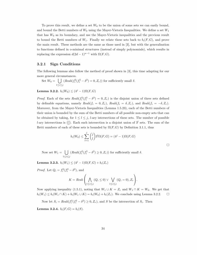
To prove this result, we define a set W0 to be the union of some sets we can easily bound,

and bound the Betti numbers of W0 using the Mayer-Vietoris Inequalities. We define a set W1

that has W0 as its boundary, and use the Mayer-Vietoris inequalities and the previous result

to bound the Betti numbers of W1. Finally we relate these sets back to bi(F, G), and prove

the main result. These methods are the same as those used in [3], but with the generalisation

to functions defined in o-minimal structures (instead of simply polynomials), which results in

replacing the expression d(2d − 1)n−1 with Ω(F, G).

3.2.1 Sign Conditions

The following lemmas also follow the method of proof shown in [3], this time adapting for our

more general circumstances. Set W0 = (Reali(fi

2(f2 − δ2) = 0, Zr)) for sufficiently small δ.i1≤i≤j

Lemma 3.2.2. bi(W0) ≤ (4j − 1)Ω(F, G)

Proof. Each of the sets Reali(fi 2(fi

2 − δ2) = 0, Zr) is the disjoint union of three sets defined

by definable equations, namely Reali(fi = 0, Zr), Reali(fi = δ, Zr), and Reali(fi = −δ, Zr). Moreover, from the Mayer-Vietoris Inequalities (Lemma 1.5.23), each of the Betti numbers of

their union is bounded by the sum of the Betti numbers of all possible non-empty sets that can

be obtained by taking, for 1 ≤ l ≤ j, l-ary intersections of these sets. The number of possible

l-ary intersections is jl . Each such intersection is a disjoint union of 3l sets. The sum of the

Betti numbers of each of these sets is bounded by Ω(F, G) by Definition 3.1.1, thus

j � �

bi(W0) ≤ � j

3lΩ(F, G) = (4j − 1)Ω(F, G)l

l=1

Now set W1 = (Reali(fi

2(f2 − δ2) ≥ 0, Zr)) for sufficiently small δ.i 1≤i≤j

Lemma 3.2.3. bi(W1) ≤ (4j − 1)Ω(F, G) + bi(Zr)

Proof. Let Qi = f2(f2 − δ2), and i i ⎛ ⎞

K = Reali ⎝ (Qi ≤ 0) ∨ (Qi = 0), Zr ⎠. 1≤i≤j 1≤i≤j

Now applying inequality (1.5.1), noting that W1 ∪ K = Zr and W1 ∩ K = W0. We get that

bi(W1) ≤ bi(W1 ∩ K) + bi(W1 ∪ K) = bi(W0) + bi(Zr). We conclude using Lemma 3.2.2.

Now let Si = Reali(fi 2(f2 − δ2) ≥ 0, Zr), and S be the intersection of Si. Then i

Lemma 3.2.4. bi(F, G) = bi(S).

34

� � �

� �

Proof. Consider a sign condition σ on F such that, without loss of generality,

σ(fi) = 0 if i = 1, . . . , j,

σ(fi) = 1 if i = j + 1, . . . , l,

σ(fi) = −1 if i = l + 1, . . . , s

and denote by Reali(σ) the subset of Zr defined by

fi(x) = 0 ∧ fi(x) ≥ δ ∧ fi(x) ≤ −δ i=1,...,j i=j+1,...,l i=l+1,...,s

It follows from Hardt’s triviality (Theorem 1.5.14) that bi(Reali(σ)) = bi(σ), with δ sufficiently

small. Note that S is the disjoint union of the Reali(σ) (for the σ realisable sign conditions) so

that σ bi(σ) = bi(S). On the other hand, σ bi(σ) = bi(F, G).

We now can prove our most substantial result

proof of Theorem 3.2.1. Using the Mayer-Vietoris Inequalities (Lemma 1.5.23), Lemma 3.2.3,

and Lemma 2.1.18 which implies, for all i < n�, bi(Zr) + bn� (Zr) ≤ b(Zr) ≤ Ω(F, G), we find

that

n�� −i � bi(S) ≤ bn� (S∅) + (4j − 1)Ω(F, G) + bi(Zr) + bn� (Zr)

j=1 J⊂{1,...,s},#(J)=j

n�� −i �≤ bn� (S∅) + 4j Ω(F, G)

j=1 J⊂{1,...,s},#(J)=j

n��−i � �s ≤ j

4j Ω(F, G)j=0

3.3 Closed Sets

In this section we prove a bound for the Betti numbers of closed (and by Alexander’s duality

open) sets. We first define closed formulae (which are used to describe closed sets), and proceed

to define sets based on these sets, slightly modified by small real numbers. We show how one can

bound the Betti numbers of the conjunction of two formulae by the sum of the Betti numbers

of the conjunction of these with a third formula that ranges over a given set, and then use this

to show how to bound the Betti numbers of a formula in terms of the sum of the Betti numbers

of some sets that are in some sense a subset of the original set. We next define sets W0 and W1

similar to those in the above section, and proceed to bound the Betti numbers of these sets.

These are then shown to be exactly related to the bounds we have found for closed formulae

above, and a bound for any closed set easily follows. Again much of the following is taken from

[3], with the same modification as above, again resulting in the introduction of Ω(F, G). We

35

� � �

�

�

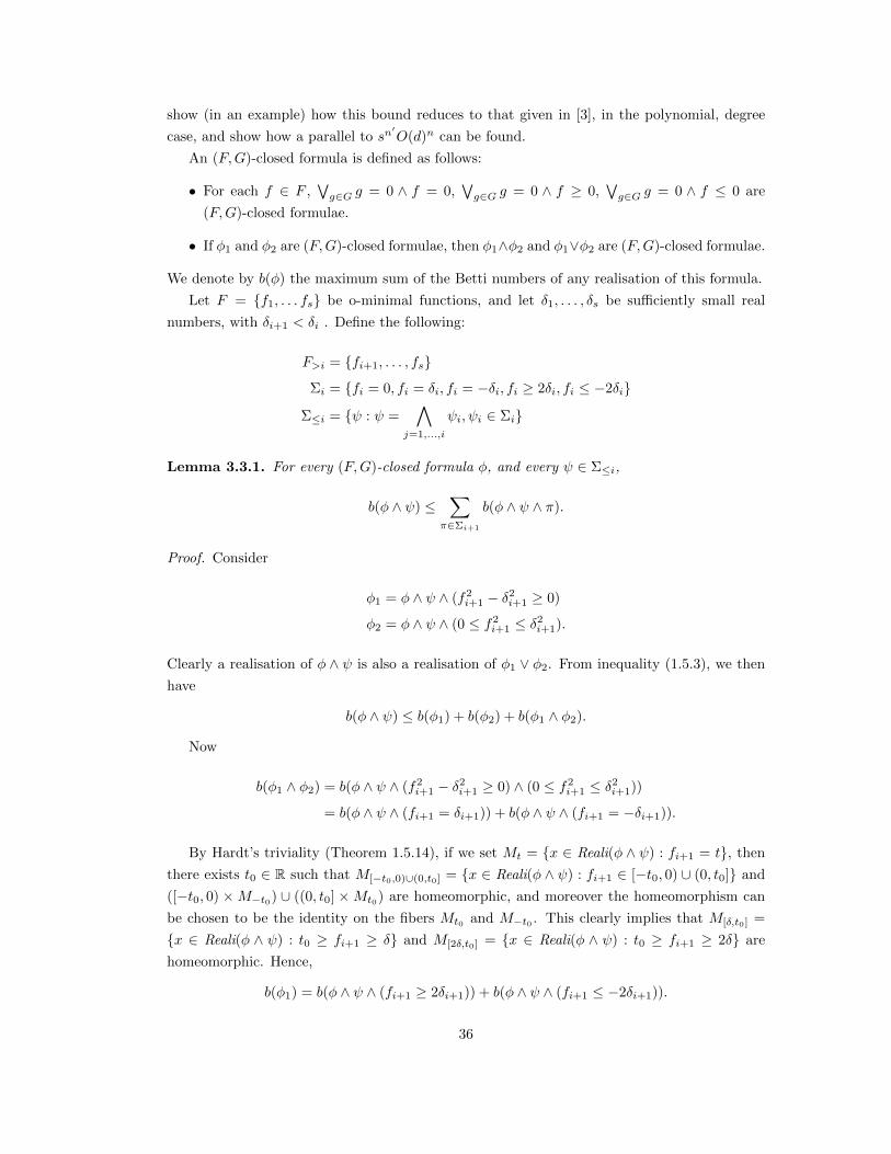
show (in an example) how this bound reduces to that given in [3], in the polynomial, degree

case, and show how a parallel to sn� O(d)n can be found.

An (F, G)-closed formula is defined as follows:

• For each f ∈ F , g∈G g = 0 ∧ f = 0, g∈G g = 0 ∧ f ≥ 0, g∈G g = 0 ∧ f ≤ 0 are

(F, G)-closed formulae.

• If φ1 and φ2 are (F, G)-closed formulae, then φ1 ∧φ2 and φ1 ∨φ2 are (F, G)-closed formulae.

We denote by b(φ) the maximum sum of the Betti numbers of any realisation of this formula.

Let F = {f1, . . . fs} be o-minimal functions, and let δ1, . . . , δs be sufficiently small real

numbers, with δi+1 < δi . Define the following:

F>i = {fi+1, . . . , fs}

Σi = {fi = 0, fi = δi, fi = −δi, fi ≥ 2δi, fi ≤ −2δi}

Σ = {ψ : ψ = ψi, ψi ∈ Σi}≤ij=1,...,i

Lemma 3.3.1. For every (F, G)-closed formula φ, and every ψ ∈ Σ≤i,

b(φ ∧ ψ) ≤ b(φ ∧ ψ ∧ π). π∈Σi+1

Proof. Consider

φ1 = φ ∧ ψ ∧ (fi2+1 − δi

2+1 ≥ 0)

φ2 = φ ∧ ψ ∧ (0 ≤ fi2+1 ≤ δi

2+1).

Clearly a realisation of φ ∧ ψ is also a realisation of φ1 ∨ φ2. From inequality (1.5.3), we then

have

b(φ ∧ ψ) ≤ b(φ1) + b(φ2) + b(φ1 ∧ φ2).

Now

b(φ1 ∧ φ2) = b(φ ∧ ψ ∧ (fi2+1 − δi

2+1 ≥ 0) ∧ (0 ≤ fi

2+1 ≤ δi

2+1))

= b(φ ∧ ψ ∧ (fi+1 = δi+1)) + b(φ ∧ ψ ∧ (fi+1 = −δi+1)).

By Hardt’s triviality (Theorem 1.5.14), if we set Mt = {x ∈ Reali(φ ∧ ψ) : fi+1 = t}, then

there exists t0 ∈ R such that M[−t0,0)∪(0,t0] = {x ∈ Reali(φ ∧ ψ) : fi+1 ∈ [−t0, 0) ∪ (0, t0]} and

([−t0, 0) × M−t0 ) ∪ ((0, t0] × Mt0 ) are homeomorphic, and moreover the homeomorphism can

be chosen to be the identity on the fibers Mt0 and M−t0 . This clearly implies that M[δ,t0] =

{x ∈ Reali(φ ∧ ψ) : t0 ≥ fi+1 ≥ δ} and M[2δ,t0] = {x ∈ Reali(φ ∧ ψ) : t0 ≥ fi+1 ≥ 2δ} are

homeomorphic. Hence,

b(φ1) = b(φ ∧ ψ ∧ (fi+1 ≥ 2δi+1)) + b(φ ∧ ψ ∧ (fi+1 ≤ −2δi+1)).

36

�

�

Note that M0 = Reali(φ ∧ ψ ∧ (fi+1 = 0)), and M[−δ,δ] = Reali(φ2). By Hardt’s Triviality

(Theorem 1.5.14), for every 0 ≤ u ≤ 1 there is a fiber-preserving homeomorphism φu from

M[−δ,−uδ] to [−δ, −uδ] × M−uδ (resp. a homeomorphism ψu from M[uδ,δ] to [uδ, δ] × Muδ). We

define a continuous homotopy m from M[−δ,δ] to M0 as follows:

• m(0, −) is limδi+1 ,

• for 0 < u ≤ 1, m(u, −) is the identity on M[−uδ,uδ] and sends M[−δ,−uδ] (resp. M[uδ,δ]) to

M−uδ (resp. Muδ) by φu (resp. ψu) followed by the projection on Muδ (resp. M−uδ ).

Thus b(M[−δ,δ]) = b(M0), and b(φ ∧ ψ) ≤ π∈Σi+1 b(φ ∧ ψ ∧ π).

Lemma 3.3.2. For every (F, G)-closed formula φ,

b(φ) ≤ b(ψ). ψ∈Σ≤s,Reali(ψ)⊂Reali(φ)

Proof. Starting from the formula φ, apply Lemma 3.3.1 with ψ the empty formula. Now,

repeatedly apply Lemma 3.3.1 to the terms appearing on the right-hand side of the inequality

obtained, noting that for any ψ ∈ Σ≤s,

• either Reali(φ ∧ ψ) = Reali(ψ) and Reali(ψ) ⊂ Reali(ψ),

• or Reali(φ ∧ ψ) = ∅.

We now use these results to prove a bound on the Betti numbers of closed sets.

Let F = {f1, . . . , fj } be o-minimal functions, and let

qi = fi 2(fi

2 − δi 2)2(fi

2 − 4δi 2).

Let W0 be the union of the set Reali(qi = 0, Zr) and W1 be the union of Reali(qi ≥ 0, Zr), with

1 ≤ i ≤ j. � Note that W1 = ψ∈Σ≤s

Reali(ψ).

Lemma 3.3.3. bi(W0) ≤ (6j − 1)Ω(F, G)

Proof. The set Reali((fi 2(f2 − δi

2)2(f2 − 4δi 2)), Zr) is the disjoint union of i i

Reali(fi = 0, Zr),

Reali(fi = δi, Zr),

Reali(fi = −δi, Zr),

Reali(fi = 2δi, Zr), and

Reali(fi = −2δi, Zr).

Moreover, the i-th Betti numbers of their union W0 is bounded by the sum of the Betti numbers

of all possible non-empty sets that can be obtained by taking intersections of these sets using

the Mayer-Vietoris Inequalities (Lemma 1.5.23).

37

� �

�

� �

�

�

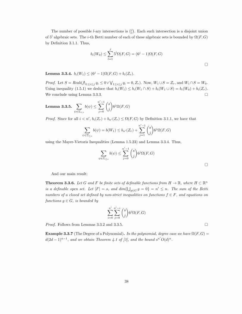
The number of possible l-ary intersections is jl . Each such intersection is a disjoint union

of 5l algebraic sets. The i-th Betti number of each of these algebraic sets is bounded by Ω(F, G)

by Definition 3.1.1. Thus,

j

bi(W0) ≤ 5lΩ(F, G) = (6j − 1)Ω(F, G) l=1

Lemma 3.3.4. bi(W1) ≤ (6j − 1)Ω(F, G) + bi(Zr).

Proof. Let S = Reali( 1≤i≤j qi ≤ 0∨ 1≤i≤j qi = 0, Zr). Now, W1 ∪S = Zr, and W1 ∩S = W0.

Using inequality (1.5.1) we deduce that bi(W1) ≤ bi(W1 ∩ S) + bi(W1 ∪ S) = bi(W0) + bi(Zr).

We conclude using Lemma 3.3.3.

� n� −1� �

Lemma 3.3.5. b(ψ) ≤ s

j 6j Ω(F, G)

ψ∈Σ<s j=0

Proof. Since for all i < n�, bi(Zr) + bn� (Zr) ≤ Ω(F, G) by Definition 3.1.1, we have that

� n�−1� �

b(ψ) = b(W1) ≤ bn� (Zr) + s

6j Ω(F, G)j

ψ∈Σ≤s j=1

using the Mayer-Vietoris Inequalities (Lemma 1.5.23) and Lemma 3.3.4. Thus,

n�−1� �� � s b(ψ) ≤

j 6j Ω(F, G)

ψ∈Σ≤s j=0

And our main result:

Theorem 3.3.6. Let G and F be finite sets of definable functions from H R, where H ⊂ Rn � →

is a definable open set. Let |F | = s, and dim{ g∈G g = 0} = n� ≤ n. The sum of the Betti

numbers of a closed set defined by non-strict inequalities on functions f ∈ F , and equations on

functions g ∈ G, is bounded by

n� n��−i � �� s 6j Ω(F, G)

ji=0 j=0

Proof. Follows from Lemmas 3.3.2 and 3.3.5.

Example 3.3.7 (The Degree of a Polynomial). In the polynomial, degree case we have Ω(F, G) =

d(2d − 1)n−1, and we obtain Theorem 4.1 of [3], and the bound sn� O(d)n .

38

�

�

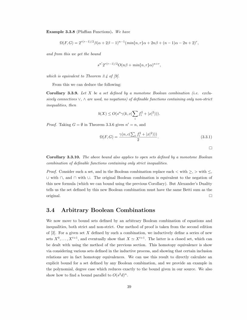
Example 3.3.8 (Pfaffian Functions). We have

Ω(F, G) = 2r(r−1)/2β(α + 2β − 1)n−1(min{n, r}α + 2nβ + (n − 1)α − 2n + 2)r ,

and from this we get the bound

s n�

2r(r−1)/2O(nβ + min{n, r}α)n+r ,

which is equivalent to Theorem 3.4 of [9].

From this we can deduce the following:

Corollary 3.3.9. Let X be a set defined by a monotone Boolean combination (i.e. exclu­

sively connectives ∨, ∧ are used, no negations) of definable functions containing only non-strict

inequalities, then

b(X) ≤ O(s nγ(k, c( fi 2 + |x|2))).

i

Proof. Taking G = ∅ in Theorem 3.3.6 gives n� = n, and

Ω(F, G) = γ(n, c( i fi

2 + |x|2))) . (3.3.1)

2

Corollary 3.3.10. The above bound also applies to open sets defined by a monotone Boolean

combination of definable functions containing only strict inequalities.

Proof. Consider such a set, and in the Boolean combination replace each < with ≥, > with ≤,

∪ with ∩, and ∩ with ∪. The original Boolean combination is equivalent to the negation of

this new formula (which we can bound using the previous Corollary). But Alexander’s Duality

tells us the set defined by this new Boolean combination must have the same Betti sum as the

original.

3.4 Arbitrary Boolean Combinations

We now move to bound sets defined by an arbitrary Boolean combination of equations and

inequalities, both strict and non-strict. Our method of proof is taken from the second edition

of [2]. For a given set X defined by such a combination, we inductively define a series of new

sets X0, . . . , Xt+1, and eventually show that X � Xt+1 . The latter is a closed set, which can

be dealt with using the method of the previous section. This homotopy equivalence is show

via considering various sets defined in the inductive process, and showing that certain inclusion

relations are in fact homotopy equivalences. We can use this result to directly calculate an

explicit bound for a set defined by any Boolean combination, and we provide an example in

the polynomial, degree case which reduces exactly to the bound given in our source. We also

show how to find a bound parallel to O(s2d)n .

39

Definition 3.4.1. Let F be a finite set of definable functions with t elements, and let S be a

bounded F -closed set.

Set SIGN(S) to be the set of realisable sign conditions of F whose realisation is contained

in S.

For σ ∈ SIGN(F ), we call the number of elements in {f ∈ F : σ(f) = 0} the level of σ.

Let ε1, ε2, . . . , ε2t−1, ε2t be sufficiently small real numbers.

We now start constructing a set that will approximate our original set. We first define the

elements that will make up this construction.

Note in the following that the c in σc stands for closed, and the o in σo stands for open. + +

Definition 3.4.2. For each level m, 0 ≤ m ≤ t, we set SIGNm(S) to be the subset of SIGN(S)

of elements of level m.

Given σ ∈ SIGNm(F, S), we set

Reali(σc ) = S ∩ {{−ε2m ≤ f ≤ ε2m for each f such that σf = 0}∪+

∪{f ≥ 0 for each f such that σf = 1}∪

∪{f ≤ 0 for each f such that σf = −1}}

and

Reali(σo ) = S ∩ {{−ε2m−1 < f < ε2m−1 for each f such that σf = 0}∪+

∪{f > 0 for each f such that σf = 1}∪

∪{f < 0 for each f such that σf = −1}}

Note that

Reali(σ) ⊂ Reali(σc ),+

Reali(σ) ⊂ Reali(σo ).+

We now define the construction of our approximating set.

Definition 3.4.3. Let X ⊂ S be a set defined on F such that X = Reali(σ)

σ∈Σ

with Σ ⊂ SIGN(S). Set Σm = Σ ∩ SIGNm(S).

We define a sequence of sets Xm ⊂ Rn for 0 ≤ m ≤ t inductively by

X0 = X•

40

� �

� �

• For 0 ≤ m ≤ t,

Xm+1 = Xm ∪ Reali(σc ) \ Reali(σo )+ +

σ∈Σm σ∈SIGNm(S)\Σm

We set X � = Xt+1 .

Theorem 3.4.4. X � X �

Before proving this, we need to introduce the following new sets, which we define inductively.

Definition 3.4.5. For each p with 0 ≤ p ≤ t + 1, we define sets Yp, Zp ⊂ Rn as follows

We set •

Y p Reali(σc )p = X ∪ +

σ∈Σp

and Zp = Y p Reali(σo )p p \ +

σ∈SIGNp(S)\Σp

• For p ≤ m ≤ t + 1 we define

Y m+1 = Y m ∪ Reali(σc ) \ Reali(σo )p p + +

σ∈Σm σ∈SIGNm(S)\Σm

and � � Zm+1 = Zm Reali(σc ) Reali(σo )p p + +∪ \

σ∈Σm σ∈SIGNm(S)\Σm

• Define Yp = Y t+1 ⊂ Rn, and Zp = Zt+1 ⊂ Rn .p p

Note that

• X = Yt+1 = Zt+1, and

• Z0 = X �.

Also note that for each p with 0 ≤ p ≤ t,

Zp+1• p+1 ⊂ Ypp, and

• Zpp ⊂ Yp

p.

The following Lemma follows directly from the above definitions of Yp and Zp.

Lemma 3.4.6. For each p with 0 ≤ p ≤ t,

• Zp+1 ⊂ Yp, and

• Zp ⊂ Yp.

41

To prove Theorem 3.4.4, it suffices to prove that the above inclusions are actually homotopy

equivalences.

Lemma 3.4.7. For 1 ≤ p ≤ t, Yp � Zp+1.

Proof. Let Yp(u) ⊂ Rn be the set obtained by replacing ε2p in the definition of Yp by u, and

for u0 > 0 define

Yp((0, u0]) = {(x, u) : x ∈ Yp(u), u ∈ (0, u0]} ⊂ Rn+1 .

By Hardt’s Triviality (Theorem 1.5.14), there exists u0 > 0 and a homeomorphism

ψ : Yp(u0) × (0, u0] Yp((0, u0])→

such that

1. πk+1(ψ(x, u)) = u,

2. ψ(x, u0) = (x, u0) for x ∈ Yp(u0),

3. for all u ∈ (0, u0] and for every sign condition σ on {f, f ± ε2t, . . . , f ± ε2p+1}

f∈F

ψ( , u) defines a homeomorphism of Reali(σ, Yp(u0)) to Reali(σ, Yp(u)).·

Now specify u0 to be ε2p, and set φ to be the map corresponding to ψ. For σ ∈ Σp, define:

Reali(σo ) = {−2ε2p < f < ε2p for all f such that σ(f) = 0}∪++

∪{f > −2ε2p for all f such that σ(f) = 1}∪

∪{f < 2ε2p for all f such that σ(f) = −1}.

Let λ : Yp → R be a continuous definable function (for example piecewise linear would suffice)

such that � • λ(x) = 1 on Yp ∩ σ∈Σp

Reali(σc ),+� λ(x) = 0 on Yp \ Reali(σo ),• σ∈Σp ++

• 0 < λ(x) < 1 otherwise.

We now consider a homotopy Yp × [0, ε2p] Yp by defining →

• h(x, t) = π1...k ◦ φ (x, λ(x)t + (1 − λ(x))ε2p) for 0 < t ≤ ε2p

• h(x, 0) = limt→0+ h(x, t) otherwise.

Note that this limit exists since S is closed and bounded. We now show that h(x, 0) ∈ Zp+1

for all x ∈ Yp. Let x ∈ Yp and y = h(x, 0). We have two cases:

42

1. λ(x) < 1. Then we have x ∈ Zp+1, and by property (3) of φ and the fact that λ(x) < 1,

y ∈ Zp+1.

2. λ(x) ≥ 1. Let σy be the sign condition of F at y, and suppose that y /∈ Zp+1. We have

two cases:

(a) σy ∈ Σ. Therefore y ∈ X, and there exists a τ ∈ SIGNm(S) \ Σm with m > p such

that y ∈ Reali(τo ).+

(b) σy ∈/ Σ. In this case, taking τ = σy , we have level(τ ) > p and y ∈ Reali(τo ). It+

follows from the definition of y and property (3) of φ that for all m > p and for all

ρ ∈ SIGNm(S):

• y ∈ Reali(ρo ) implies that x ∈ Reali(ρo )+ +

• x ∈ Reali(ρc ) implies that y ∈ Reali(ρc )+ +

Thus x /∈ Yp, a contradiction.

It follows that:

• h(·, ε2p) : Yp → Yp is the identity,

• h(Yp, 0) = Zp+1, and

• h(·, t) restricted to Zp+1 gives a homotopy between

h(·, ε2p)|Zp+1 = idZp+1

and

h(·, 0)|Zp+1 .

Thus Yp � Zp+1.

Lemma 3.4.8. For all p with 0 ≤ p ≤ t, Zp � Yp.

Proof. For this proof define the following new sets for u ∈ R:

Z � (u) ⊂ Rn is the set obtained by replacing in the definition of Zp, ε2j by ε2j − u, and • p

ε2j−1 by ε2j−1 + u for all j > p, and ε2p by ε2p − u and ε2p−1 by u.

For all u0 > 0, define

Z � ((0, u0]) = {(x, u) : x ∈ Z � (u), u ∈ (0, u0]}.p p

• Let Yp�(u) ⊂ Rn be the set obtained by replacing in the definition of Yp, ε2j by ε2j − u

and ε2j−1 by ε2j−1 + u for all j > p, and ε2p by ε2p − u.

• For σ ∈ SIGNm(S) with m ≥ p, let Reali(σc )(u) ⊂ Rn denote the set obtained by +

replacing ε2m by ε2m − u in the definition of Reali(σc ).+

43

• For σ ∈ SIGNm(S) with m > p, let Reali(σo )(u) ⊂ Rn denote the set obtained by +

replacing ε2m−1 by ε2m−1 + u in the definition of Reali(σo ).+

• Finally, for σ ∈ SIGNp(S), let Reali(σo )(u) ⊂ Rn denote the set obtained by replacing +

ε2p−1 by u in the definition of Reali(σc ).+

Note that by the definitions, for all u, v ∈ R with 0 < u ≤ v, Z � (u) ⊂ Yp�(u), Z � (v) ⊂ Z � (u),p p p

Yp�(v) ⊂ Yp

�(u), and Yp

�(s) = Zp� (s).

0<s≤u 0<s≤u

Let Zp� = Zp

� (ε2p−1) and Yp� = Yp

�(ε2p−1). It is easy to see that Yp� � Yp, and Zp

� � Zp. We will

now prove that Yp� � Z � , which suffices to prove the Lemma. p

Let µ : Yp� → R be a definable map with

µ(x) = supu∈(0,ε2p−1 ]{u : x ∈ Zp� (u)}.

We will prove below (Lemma 3.4.9) that µ is continuous. Note that the definition of Zp� (u)

(as well as Yp�(u)) is more complicated than the natural one consisting of replacing ε2p−1 in

the definition of Zp by u, due to the fact that with the latter definition µ is not necessarily

continuous.

We now construct a definable map

h : Yp� × [0, ε2p−1] → Yp

�

as follows. By Hardt’s Triviality (Theorem 1.5.14) there exists u0 > 0 and a homeomorphism

ψ : Z � (u0) × (0, u0] → Z � ((0, u0])p p

such that:

1. πk+1(ψ(x, u)) = u,

2. ψ(x, u0) = (x, u0) for x ∈ Z � (u0),p

3. for all u ∈ (0, u0] and for all sign conditions σ of {f, f ± ε2t, . . . , f ± ε2p+1},

f ∈F

the map ψ( , u) restricts to a homeomorphism of Reali(σ, Zp� (u0))·

to Reali(σ, Zp� (u)).

Now specify that u0 = ε2p−1, and denote by φ the corresponding map

φ : Zp� × (0, ε2p−1] → Zp

� ((0, ε2p−1]).

44

Note that for all u with 0 < u ≤ ε2p−1, φ gives a homeomorphism

φu : Zp� (u) Zp

� .→

Hence for every pair u, u� with 0 < u ≤ u� ≤ ε2p−1, there exists a homeomorphism

θu,u� : Zp� (u) Zp

� (u�)→

obtained by composing φu with φ−1 . For 0 ≤ u� ≤ u ≤ ε2p−1, let θu,u� be the identity map. It u�

is clear that θu,u� moves continuously with u and u�.

For x ∈ Yp� and t ∈ [0, ε2p−1], now define

h(x, t) = θµ(x),t(x).

It is easy to verify from the definition of h and the properties of φ above that h is continuous

and:

• h(·, 0) : Yp� → Yp� is the identity map

• h(Yp�, ε2p−1) = Z � ,p

• h(·, t) restricts to a homeomorphism Zp� × t → Zp

� for every t ∈ [0, ε2p−1].

Thus, Zp � Yp

Lemma 3.4.9. For sufficiently small ε2p−1, the definable map µ : Yp� → R defined by

µ(x) = supu∈(0,ε2p−1]{u : x ∈ Zp� (u)}

is continuous.

Proof. In order to prove the continuity of µ we show that for every point x� ∈ Yp�, for all εµ > 0

there exists δµ > 0 such that for all x ∈ Yp� with |x − x�| < δµ we have |µ(x) − µ(x�)| < εµ.

Choose εµ. Since each function f ∈ F is continuous, setting ε := εµ/2 in the standard

definition of continuity, for each f there exists δf > 0 such that if |x − x�| < δf then |f(x) −

f(x�)| < εµ/2. Set δµ = minf∈F {δf } , and fix x and x� with |x − x�| < δµ. Let u ∈ (0, ε2p−1] be

such that x ∈ Z � (u). We show below that this implies that x� ∈ Z � (u�) for some u� satisfyingp p

|u − u�| < εµ.

Let m be the largest integer such that there exists σ ∈ Σm with x ∈ Reali(σc )(u): since+

x ∈ Zp� (u) such an m must exist. We have two cases:

1. m > p: Let σ ∈ Σm with x ∈ Reali(σc )(u). Then by maximality of m, for all +

f with σ(f) = 0 we have f(x) = 0. Therefore x� ∈ Reali(σc )(u�) for all u� <∈ F � � +

u − maxf∈F,σ(f )=0|f(x) − f(x�)| ≤ u − εµ/2 . We can thus choose u� such that x� ∈

Reali(σc )(u�) and < εµ.+ |u − u�|

45

2. m ≤ p: If x� ∈/ Zp� (u) then since x� ∈ Yp� ⊂ Yp

�(u), Reali(σo )(u).x� ∈ +

σ∈SIGNp(F,S)\Σp

Let σ ∈ SIGNp(S) \ Σp be such that x� ∈ Reali(σo )(u). We prove by contradiction that +

maxf ∈F,σ(f)=0|f(x�)| = u.

Assume the contrary. Since x ∈/ Reali(σo )(u) by assumption, and < εµ, there + |x − x�|must exist f ∈ F with σ(f) =� 0 and f(x) = 0. Letting τ denote the sign condition

defined by τ (f) = 0 if f(x) = 0 and τ(f) = σ(f) otherwise, we have that level(τ) > p

and x belongs to both Reali(τ o )(u) and Reali(τ c )(u). Now there are two cases: + +

(a) τ ∈ Σ: then the fact that x ∈ Reali(τ c )(u) contradicts the choice of m, since m ≤ p+

and level(τ) > p.

(b) τ /∈ Σ: then x gets removed at the level of τ in the construction of Z � (u), and hence p

x ∈ Reali(ρc )(u) for some ρ ∈ Σ with level(ρ) > level(τ) > p. This again contradicts +

the choice of m.

Thus, maxf ∈F,σ(f)=0|f(x�)| = u, and since x� ∈/ Reali(σo )(u�)+

σ∈SIGNp(C,S)\Σp

for all � u� < maxf∈F,σ(f )=0|f(x�)| = u, we can choose u� such that |u − u�| < εµ and

x� / Reali(σo )(u�).σ∈SIGNp(F,S)\Σp +∈

In both cases we have x� ∈ Zp� (u�) for some u� satisfying |u − u�| < εµ. This means for x ∈ Yp

�

and u with x ∈ Zp� (u), and for x� with |x� − x| < δµ, there exists u� with x� ∈ Zp

� (u�), with

u� < u and |u − u�| < εµ. We therefore have µ(x) − µ(x�) < εµ. Reversing the roles of x and x�

in the above, we get µ(x�) − µ(x) < εµ. Hence |µ(x) − µ(x�)| < εµ, and µ is continuous.

Proof of Theorem 3.4.4. This follows from Lemmas 3.4.7 and 3.4.8.

Corollary 3.4.10. Let Y ⊂ Rn be a set defined by a Boolean combination of definable functions

{f1, . . . , fs}. Then there exists a closed set X ⊂ Rn defined by 2s2 + 1 definable functions with

complexities c(fi), and c(|x|) such that X � Y .

Theorem 3.4.11. Let Y ⊂ Rn be a set defined by a Boolean combination of definable functions

{f1, . . . , fs}. Then n n−i� ��� 2s2 + 1

b(Y ) ≤ j

6j Ω(F �, ∅) i=0 j=1

where F � contains all the elements fi and |x|2 .

46

�

� � � � �� �

� � �

� �

� �

Example 3.4.12 (The Degree of a Polynomial). We have Ω(F �, ∅) = d(2d − 1)n−1, and we

obtain Theorem 7.50 of the second edition of [2].

Example 3.4.13 (Pfaffian Functions). We have

Ω(F �, ∅) = 2r(r−1)/2β(α + 2β − 1)n−1(min{n, r}α + 2nβ + (n − 1)α − 2n + 2)r ,

and we get

n � �� n−i 2s2 + 1 b(Y ) ≤

j 6j 2r(r−1)/2β(α + 2β − 1)n−1 ·

i=0 j=1

(min{n, r}α + 2nβ + (n − 1)α − 2n + 2)r .·

Corollary 3.4.14.

b(Y ) ≤ O s 2nΩ(F �, ∅)

≤ O s 2nγ n, c( fi 2 + |x|2)

i

Proof. As in 3.3.9.

Example 3.4.15 (The Degree of a Polynomial). We have

γ n, c( f2 + |x|2) = 2d(2d − 1)n−1 ,i i

and we get the bound O((s2d)n).

Example 3.4.16 (Pfaffian Functions). We get a bound

b(X) ≤ O s 2n2r(r−1)/2β(α + 2β − 1)n−1(min{n, r}α + 2nβ + (n − 1)α − 2n + 2)r

≤ O s 2n2r(r−1)/2(α + 2β)n(min{n, r}α + 2nβ + (n − 1)α − 2n + 2)r

≤ O(s 2n2r(r−1)/2(2nβ + (min{n, r} + n − 1)α)n+r),

which is equivalent to the bound stated in [22].

47

Chapter 4

Sets Defined with Quantifiers

4.1 Introduction

We now move on to tackle the most general situation, where X is a subset in [−1, 1]n0 ⊂ Rn0

defined by

X = {x0 : Q1x1Q2x2 . . . Qν xν ((x0, x1, . . . , xν ) ∈ Xν )}, (4.1.1)

where Qi ∈ {∃, ∀}, Qi =� Qi+1, xi ∈ Rni , and Xν is some definable set in [−1, 1]n0 +...+nν .

Example 4.1.1. If ν = 1 and Q1 = ∃, then X is the projection of X1.

We make use of existing methods and ideas from two main sources in our new setting, as

outlined below.

In [12], the authors present a method for bounding the Betti numbers of a surjective map

using a particular spectral sequence. They then proceed to demonstrate how to bound the

Betti numbers of a set of the form (4.1.1), in the case where Xν is open or closed and is the

difference between a finite CW-complex and its subcomplex. To achieve this, they firstly state

forms of well-known results such as Alexander’s Duality (which considers complements), the

Mayer-Vietoris Inequality (which deals with unions and intersections), and De Morgan’s Law.

They also introduce a form of notation to manipulate various specific unions/intersections.

These ideas are then used, along with the fact that the existential quantifier is equivalent to

projection, to transform the problem into a form that can be solved using the spectral sequence

method applied to the projection map. Finally, upper bounds for sub-Pfaffian sets are found by

simply counting the number of terms in the expression resulting from the above, and directly

calculating the complexity of the summand.

In [11], a method is shown to approximate a given definable set by a compact family T ,

based on sets that “represent” the given set. This “representation” is axiomatically defined,

and a particular case of “representation” is constructed in the setting of a bounded definable

set of points satisfying a Boolean combination of equations and inequalities. This result is then

used to demonstrate how to improve existing bounds on Betti numbers of sub-Pfaffian sets,

48

both in the quantifier-free case, and, making use of the spectral sequence result above, in the

case of a single projection.

My work seeks to combine the above ideas to produce a bound for any definable set of the

form (4.1.1), in terms of the general complexity definition I give at the beginning of this work.

I proceed by presenting various parts of the two above papers, adapted to my new context, and

generalised to give the desired result.

Note that early results for semi-Pfaffian sets defined by quantifier-free formulae (see [22])

required the set to be restricted, i.e. closure(X) ⊂ (0, 1)n; this requirement was removed in

[11]. Similarly, the method shown in [12] requires the quantifier-free part of the set to be open

or closed. Because our result uses the construction of a compact representation as above, which

guarantees that the closed set T ⊂ (0, 1)n, we can remove this restriction and produce a result

for any set definable in an o-minimal structure over the reals, in particular, including those

defined using quantifiers.

4.2 Sidenote – the case where Xν is open or closed

In [12] a bound is given in terms of a summation of sets (an analogue to Theorem 4.9.8) in the

case where Xν is open or closed, and is the difference between a finite CW-complex and one

of its subcomplexes. Our new axiomatic complexity measure can be applied to this bound to

produce an explicit bound for sets defined in o-minimal structures. It is a simple calculation to

show that this bound reduces to the results given in [12] in the polynomial and Pfaffian cases.

In the following we produce bounds that are weaker the above. This is due to the fact that

Xν need not be open or closed, and not due to the new complexity metric.

4.3 A Spectral Sequence Associated with a Surjective Map

We now describe how to associate a particular mathematical object with a given surjective

map; this in particular allows us to bound the Betti numbers of the codomain of this map. We

will use this result later in the instance of projection maps. The mathematical object used is a

spectral sequence; a good introduction to spectral sequence can be found in [5].

This section is taken directly from [12].

Definition 4.3.1. A continuous map f : X Y is locally split if for any y ∈ Y there is an →

open neighbourhood U of y and a section s : U X of f (i.e., s is continuous and fs = Id).→

In particular, a projection of an open set in Rn on a subspace of Rn is always locally split.

Definition 4.3.2. For two maps f1 : X1 → Y and f2 : X2 → Y , the fibered product of X1 and

X2 is defined as

X1 ×Y X2 = {(x1, x2) ∈ X1 × X2 : f1(x1) = f2(x2)}.

Theorem 4.3.3. Let f : X Y be a surjective cellular map. Assume that f is either closed →

or locally split. Then for any Abelian group G, there exists a spectral sequence Er converging p,q

49

�

�

to H∗(Y, G) with

E1 = Hq (Wp, G)p,q

where

Wp . . . ×Y X .= X� ×Y �� � p+1 times

In particular,

dim Hk(Y, G) ≤ dim Hq(Wp, G), p+q=k

for all k.

Proof. See [12], Theorem 1.

4.4 Alexander’s duality

Again the following is taken from [12].

Let

Iin = .{−i ≤ xj ≤ i} ⊂ Rn

1≤j≤n

Define the “thick boundary” ∂Iin = Ii

n +1\Iin . The following is a version of Alexander’s

duality theorem.

Lemma 4.4.1 (Alexander’s duality). If X ⊂ In is an open set in Iin, then for any q ∈ Z,i

q ≤ n − 1,

Hq (Iin\X, R) ∼ Hn−q−1(X ∪ ∂In (4.4.1)= i , R).

If X ⊂ In is a closed set in Iin, then for any q ∈ Z, q ≤ n − 1,i

Hq (Iin\X, R) ∼ Hn−q−1(X ∪ closure(∂In (4.4.2)= i ), R).

Proof. See [12], Lemma 4.

4.5 Approximation of Definable Sets by Compact Fami­

lies

We now outline the methods shown in [11] to find a compact set to approximate an arbitrary

set, which can belong to a large class of definable sets, including sets defined by any Boolean

combination of equations and inequalities.

We take the following Definition and two Lemmas directly from [11]:

Definition 4.5.1. Let G be a definable compact set. Consider a definable family {Sδ}δ>0

of compact subsets of G such that, for all δ�, δ ∈ (0, 1), if δ� > δ, then Sδ� ⊂ Sδ . Denote � S := δ>0 Sδ .

50

�

For each δ > 0, let {Sδ,ε}δ,ε>0 be a definable family of compact subsets of G such that:

(i) for all ε, ε� ∈ (0, 1), if ε� > ε, then Sδ,ε ⊂ Sδ,ε� ;

(ii) Sδ = ε>0 Sδ,ε;

(iii) for all δ� > 0 sufficiently smaller than δ, and for all ε� > 0, there exists an open in G set

U ⊂ G such that Sδ ⊂ U ⊂ Sδ�,ε� .

We say that S is represented by the families {Sδ}δ>0 and {Sδ,ε}δ,ε>0 in G.

Let S� be represented by {Sδ� }δ>0 and {S�δ }δ>0δ,ε}δ,ε>0 in G, and let S�� be represented by {S��

and {S��δ,ε}δ,ε>0 in G.

Lemma 4.5.2. The set S� ∩S�� is represented by the families {Sδ� ∩Sδ��}δ>0 and {S�δ,ε}δ,ε>0δ,ε ∩S��

in G, while S� ∪ S�� is represented by {Sδ� ∪ Sδ��}δ>0 and {S�

δ,ε}δ,ε>0 in G.δ,ε ∪ S��

Proof. By checking of Definition 4.5.1.

Let S be represented by {Sδ}δ>0 and {Sδ,ε}δ,ε>0 in G, and let F : D H be a continuous →

definable map, where D and H are definable, S ⊂ D ⊂ G, and H is compact.

Lemma 4.5.3. Let D be open in G, and F be an open map. Then F (S) is represented by the

families {F (Sδ)}δ>0 and {F (Sδ,ε)}δ,ε>0 in H.

Proof. Follows from checking Definition 4.5.1; openness is required for (iii) to hold.

In [11], this general case is called the definable case (i.e. it has been axiomatically defined).

A more specific case is actually constructed (in [11]) in the situation of a set defined by a

Boolean combination of equations and inequalities, and is referred to as the constructible case.

We outline this now, again taking the following directly from [11].

Let S = {x : F(x)} ⊂ Rn be a bounded definable set of points satisfying a Boolean

combination F of equations of the kind h(x) = 0 and inequalities of the kind h(x) > 0, where

h : Rn R are continuous definable functions (e.g. polynomials). As G take a closed ball of →

sufficiently large radius centred at 0. We now define the representing families {Sδ} and {Sδ,ε}.

Definition 4.5.4. For a given finite set {h1, . . . , hk} of functions hi : Rn R, define its sign→

set as a non-empty subset in Rn of the kind

hi1 = . . . = hik1 = 0, hik1+1 > 0, . . . , hik2

> 0, hik2+1 < 0, . . . hik < 0,

where i1, . . . , ik1 , . . . , ik2 , . . . , ik is a permutation of 1, . . . k.

Let now {h1, . . . hk} be the set of all functions in the Boolean formula defining S. Then S

is a disjoint union of some sign sets of {h1, . . . hk}. The set Sδ is the result of the replacement,

independently in each sign set in this union, of all inequalities h > 0 and h < 0 by h ≥ δ and

h ≤ −δ respectively. The set Sδ,ε is obtained by replacing all expressions h > 0, h < 0, and

51

h = 0 by h ≥ δ, h ≤ −δ and −ε ≤ h ≤ ε respectively. According to Lemma 4.5.2, the set S

being the union of sign sets, is represented by the families {Sδ} and {Sδ,ε} in G.

Now suppose that the set S ⊂ Rn, defined as above by a Boolean formula F , is not necessar­

ily bounded. In this case as G take the definable one-point (Alexandrov) compactification of Rn .

Note that each function h is continuous in G \ {∞}. Define sets Sδ and Sδ,ε as in the bounded

case, replacing equations and inequalities, independently in each sign set of {h1, . . . , hk}, and

then taking the conjunction of the resulting formula with |x|2 ≤ 1/δ. Again, S is represented

by {Sδ} and {Sδ,ε} in G.

We now return to the more general, definable, case. The following Definitions and Lemma

are taken from [11], with a slight modification of notation to indicate that T depends on the

family chosen to represent S, and on the value m (as defined below).

Definition 4.5.5. For a sequence ε0, δ0, ε1, δ1, . . . , εm, δm, where m ≥ 0, and a particular

representation Υ = {Sδ,ε}δ,ε>0 of S, introduce the compact set

TΥ,m(S) := Sδ0,ε0 ∪ Sδ1 ,ε1 ∪ . . . ∪ Sδm,εm .

In the following, see Definition 1.5.22 for the � symbol.

Lemma 4.5.6. For any m ≥ 0, for

0 < ε0 � δ0 � ε1 � δ1 � . . . � εm � δm � 1 (4.5.1)

and for a representation Υ of S, there is a surjective map C : T S from the finite set T of→

all connected components of TΥ,m(S) onto the set S of all the connected components of S such

that, for any S� ∈ S, we have T � = TΥ,m(S�).

T �∈C−1(S�)

If m > 0, then C is bijective.

Proof. The surjectivity follows directly from Definition 4.5.1. Bijectivity is proven in Lemma

1.4 of [11].

The previous Lemma essentially states that the passage to TΥ,m preserves connectivity. The

next Theorem is essentially the key result in [11], and is again taken directly.

In the remained of this document, we denote T := TΥ,m(S) whenever this does not lead to

confusion.

We assume m > 0, and that S is connected in order to make the homotopy groups πk(S)

and πk(T ) independent of a base point.

Theorem 4.5.7. For a given representation Υ of S:

52

(i) For (4.5.1) and for every 1 ≤ k ≤ m, there are epimorphisms

ψk : πk(T ) πk(S),→

φk : Hk(T ) Hk(S),→

and, in particular, rank Hk(S) ≤ rank Hk(T ).

(ii) In the constructible case, for (4.5.1) and for every 1 ≤ k ≤ m − 1, ψk and φk are

isomorphisms, in particular rank Hk(S) = rank Hk(T ). Moreover, if m ≥ dim(S), then

T � S.

Proof. See [11], Theorem 1.5.

Note that in the above Theorem πk refers to homotopy groups, not projections. The fol­

lowing Corollary is the direct implication of this existing work in our new setting, and is the

only original item in this section.

Corollary 4.5.8. Let S ⊂ Rn be defined by an arbitrary Boolean combination of s distinct

definable functions hi, with maximum complexity max(c(hi)). Then there exists a compact

set T ⊂ Rn defined by a Boolean combination (with no negations) of 4(n + 1)s non-strict

inequalities, with maximum complexity max(c(hi), c(|x|2)), with T � S.

4.5.1 Projections

To move towards dealing with quantifiers, we take a first look at how to deal with projections.

This section is expanded on in more detail later, we only touch on it now to show how the

previous work can be applied in our new setting. In the following definition, we show that

T (π(S)) can indeed be defined in the natural way.

Definition 4.5.9. Let π : Rn+r → Rn be the projection function, and S ⊂ Rn+r . The set S

is represented by the families {Sδ }δ and {Sδ,ε}δ,ε in the compactification of Rn+r as described

above. According to Lemma 4.5.3, the projection π(S) is represented by the families {π(Sδ)}δ

and {π(Sδ,ε)}δ,ε in the compactification of Rn, we call this particular representation Π. Fix

m = n + r. Then for a given representation Υ of S, we can define π(TΥ,m(S)) to be equal to

TΠ,m(π(S)).

We now demonstrate how this can be applied in the constructible case to give a bound

using our general complexity definition, analogous to bounds given in [11] for the polynomial

(complexity = degree) case, and for the Pfaffian case. Let S = {(x, y) : F(x, y)} ⊂ Rn+r, where

F is a Boolean combination of definable equations and inequalities of the kind hi(x, y) = 0 or

hi(x, y) > 0, where hi are definable functions (1 ≤ i ≤ s). Suppose that the maximum

complexity of these functions is max(c(hi)).

53

� � �

�

� �� �

� � �

� � � �

� � �� �

Lemma 4.5.10.

� k3 + 4k2 + 5k + 2

�n+(k+1)r ⎛ � � ��

2

��⎞

bk(π(S)) ≤ 2

s O ⎝ γ n + (p + 1)r, c hi 2 + |x| ⎠

i0≤p≤k

Proof. For k = 0, we have b0(π(S)) ≤ b0(S). Lemma 4.5.6 tells us that there exists a surjective

map from the set of connected components of TΥ,m(S) to the set of connected components of

S, and therefore b0(S) ≤ b0(TΥ,m(S)). The set TΥ,m is defined by 4(k + 1)s definable functions

and is in Rn, hence, by Corollary 3.3.9, b0(TΥ,m(S)) ≤ O snγ(n, c( i h2 i + |x|2)) .

Now assume k > 0, and fix m = k. From Definition 4.5.9, we have TΠ,m(π(S)) =

π(TΥ,m(S)), and recall from Section 1.5.6 that bi(X) = rank Hi(X). According to Theorem

4.3.3, we have

bk(π(TΥ,m(S))) ≤ bq(Wp), p+q=k

where

Wp = TΥ,m(S) ×π(TΥ,m(S)) . . . ×π(TΥ,m(S)) TΥ,m(S) .

p+1 times

The fibre product Wp ⊂ Rn+(p+1)r is definable by a Boolean formula with

4(p + 1)(k + 1)s

o-minimal functions. Hence, by Corollary 3.3.9, we have

bq(Wp) ≤ O ((p + 1)(k + 1)s)n+(p+1)rγ(n + (p + 1)r, c( h2 i + |x|2)) .

i

It follows that

bk(TΠ,m(π(S))) ≤ O ((p + 1)(k + 1)s)n+(p+1)rγ(n + (p + 1)r, c( hi 2 + |x|2))

0≤p≤k i ⎛ ⎞ � k3 + 4k2 + 5k + 2

�n+(k+1)r � � ≤

2 s O ⎝ γ(n + (p + 1)r, c( h2

i + |x|2))⎠ . 0≤p≤k i

Finally, by Theorem 4.5.7, bk(π(S)) ≤ bk(TΠ,m(π(S))), and the result follows.

Example 4.5.11 (The Degree of a Polynomial). In the case of polynomials and degree, we

have

γ n + (p + 1)r, c hi 2 + |x|2 ≤ O(dn+(p+1)r),

i

and therefore bk(π(S)) ≤ ((k + 1)sd)O(n+kr), which is the result given in [11] Theorem 6.4.

54

� � �� �

Example 4.5.12 (Pfaffian Functions). In this case we have

γ n + (p + 1)r, c h2 + |x|2 ≤ O(2r 2

((n + (p + 1)r)(α + β))n+(p+1)r)ii

and therefore

bk(π(S)) ≤ (ks)O(n+(k+1)r)2(kl)2

((n + (k + 1)r)(α + β))n+(k+1)r+kl ,

which is the result given in [11] Theorem 6.8.

4.6 Notation

In the following, remember A means the complement of A. Existing work ([12]) defines an

initial set X, and proceeds to define sets Xi that fit the relation π(Xi) = Xi−1, and uses this

recurrence later in the inductive proof of the main result. However, in this setting we must

define things slightly differently, as we are using the concept of “representation”, and we must

be able to find a set to “represent” the set in the recurrence relation. This requires the map

to be open, and the complement of the projection does not necessarily take open sets to open

sets. We can circumvent this difficulty by using projection and co-projection (complement of

the projection of the complement) in our definition, as they are both open maps (i.e. take open

sets to open sets). We therefore use the slightly more cumbersome notation that follows, where

later work will come to depend on the parity of i.

We assume that X ⊂ [−1, 1]n0 ⊂ Rn0 , and Xν ⊂ [−1, 1]n0+...+nν . To restate our original

formula, we have

X = {x0 : Q1x1Q2x2 . . . Qν xν ((x0, x1, . . . , xν ) ∈ Xν )}, (4.6.1)

where Qi =� Qi+1. We will also assume that Q1 = ∃, the other case can be dealt with using

Alexander’s Duality (and is explicitly dealt with later using another method in the case of

exactly one universal quantifier).

Let π(S) be denoted by cp(S). We now define sets

Xi = {(x0, . . . , xi) : Qi+1xi+1Qi+2xi+2 . . . Qν xν ((x0, x1, . . . , xν ) ∈ Xν )}.

55

This definition satisfies

X = X0

= π1(X1)

= π1(cp2(X2))

= π1(cp2(π3(X3)))

. . .

= π1(cp2(π3(. . . (τi(Xi))))),

where τi = πi if i is odd, and τi = cpi if i is even. Essentially this notation gives identical sets

to the existing notation for odd i, and the complement of previous sets for even i.

For a set Imi mi−1 × . . . × Im1 , define ∂(Imi mi−1 × . . . × Im1 ) as i × Ii−1 1 i × Ii−1 1

(Imi mi−1 × . . . × Im1 )\(Imi mi−1 × . . . × Im1 )i+1 × Ii 2 i × Ii−1 1

for even i, and as the closure of this difference for odd i.

Let p1, . . . , pi be some positive integers to be defined later. Define

Bii = ∂(In0 +(p1+1)n1 × I(p2+1)n2 × . . . × I1

(pi−1+1)ni−1 ) × I1 ni .i−1 i−2

For any j, i < j ≤ ν, define Bi = Bji −1 × Inj , where complements are in appropriate cubes. j 1

4.6.1 General Intersections and Unions

We now define an “intersection” of particular types of sets, again taking all Definitions and

Lemmas in this section directly from [12].

Definition 4.6.1. (i) Let Y ⊂ In0 (p1+1)n1 (p2+1)n2 × . . . × I(pl−1+1)nl−1 × Inl+...+ni ,v × Iv × Iv−1 ν−l+2 1

where 1 ≤ l ≤ i, v ≥ i, and let J ⊂ {(jl, . . . , ji) : 1 ≤ jk ≤ pk + 1, l ≤ k ≤ i}. Then define �l

Y as an intersection of sets i,J

{(x0, x(1), . . . , x(p1+1), . . . , x

(1), . . . , x

(pi+1)) : 1 1 i i

x0 ∈ In0 , x(m) ∈ Ink (1 ≤ k ≤ l − 1),v k v−k+1

(m) (1) (pl−1 +1) (jl ) (ji)xk ∈ I1 nk (l ≤ k ≤ i), (x0, x1 , . . . , xl−1 , xl , . . . , xi ) ∈ Y }

over all (jl, . . . , ji) ∈ J .

(p1+1)n1 (p2+1)n2 (pl−1+1)nl−1 nl+...+ni+ni+1(ii) Let Y ⊂ In0 × I × Iv−1 × . . . × I × I . Define �l,i+1

Yv v ν−l+2 1 i,J

56

�

�

as an intersection of sets

{(x0, x(1), . . . , x(p1+1), . . . , x

(1), . . . , x

(pi+1), xi+1) : 1 1 i i

x0 ∈ In0 , x(m) ∈ Ink (1 ≤ k ≤ l − 1), x(m) ∈ Ink

v k v−k+1 k 1 (l ≤ k ≤ i), ni+1 (1) (pl−1 +1) (jl ) (ji)xi+1 ∈ I1 , (x0, x1 , . . . , xl−1 , xl , . . . , xi ) ∈ Y }

over all (jl, . . . , ji) ∈ J .

(iii) If l = i and J = {j : 1 ≤ j ≤ pi + 1} we use the notation �i

Y for �i

Yi i,J

The following shows how these intersections combine:

Lemma 4.6.2. Let

Y ⊂ In0 × I(p1+1)n1 (p2+1)n2 × . . . × I(pl−1 +1)nl−1 nl+...+ni+ni+1 .v v × Iv−1 v−l+2 × I1

Then for any J ⊂ {j : 1 ≤ j ≤ pi+1 +1}, J � ⊂ {(jl, . . . , ji) : 1 ≤ jk ≤ pk +1, l ≤ k ≤ i} we have

i+1 l,i+1 l� � Y =

� Y.

i+1,J i,J� i+1,J �×J

Proof. Straightforward.

We similarly define unions: ��l ��l,i+1Definition 4.6.3. Let Y , l, i, J be as in Definition 4.6.1. Define i,J Y and i,J Y similar

to �l

Y and �l,i+1

Y respectively, replacing in Definition 4.6.1 “intersection” by “union”. i,J i,J

We now state a version of De Morgan’s law, which show how unions, intersections, and

complements interact.

Lemma 4.6.4 (De Morgan’s Law). ⎛ ⎞ l l⎝� ⎠Y = Y i,J i,J

⎛ ⎞ l,i+1 l,i+1⎝

� ⎠Y = Y i,J i,J

where complements are in appropriate cubes.

Proof. Straightforward.

We now define projections:

57

� �

�

Definition 4.6.5. Let ti = n0 + n1(p1 + 1) + . . . + ni(pi + 1). Define projection maps

πi : Rn0+...+ni Rn0+...+ni−1 →

(x0, . . . , xi) �→ (x0, . . . , xi−1)

and for j < i,

πi,j : Rtj +nj+1+...+ni Rtj +nj+1+...+ni−1 →

(x0, x(1), . . . , x

(pj +1), xj+1, . . . , xi) �→ (x0, x

(1), . . . , x

(pj +1), xj+1, . . . , xi−1).1 j 1 j

We finally show how unions and projections commute

Lemma 4.6.6. Let

× I(p1+1)n1 (p2+1)n2 (pl−1 +1)nl−1 nl+...+ni+ni+1Y ⊂ Ivn0

v × Iv−1 × . . . × Iv−l+2 × I1 .

Then ⎛ ⎞ l l,i+1

πi+1,l−1(Y ) = πi+1,i ⎝ Y ⎠ . i,J i,J

Proof. Straightforward.

4.7 Application of Spectral Sequence Result

We present a Lemma that will allow us to use Theorem 4.3.3 in our proof.

(p1+1)n1 (p2+1)n2 (pi−1+1)ni−1Lemma 4.7.1. For any closed A ⊂ Ivn0 × Iv × Iv−1 × . . . × Iv−i+2 × I1

ni ,

� i

bk(πi,i−1(A)) ≤ bqi (�

(A)). pi+qi=k i

Proof. Theorem 4.3.3 tells us that

bk(Y ) ≤ bq(Wp). p+q=k

We will take Y = πi,i−1(A), and f = πi,i−1. For convenience, let us say I = Ivn0 × Iv

(p1+1)n1 ×(p2+1)n2 (pi−1+1)ni−1Iv−1 × . . . × Iv−i+2 so A ⊂ I × I1

ni , so we have πi,i−1(A) ⊂ I.

From the definition,

Wpi = {((a, b1), (a, b2), . . . , (a, bpi+1) : a ∈ I, bj ∈ Ini , (a, bj ) ∈ A, 1 ≤ j ≤ pi + 1}.1

Similarly, we have

i�(A) = {(a, b1, b2, . . . , bpi+1) : a ∈ I, bj ∈ Ini , (a, bj ) ∈ A, 1 ≤ j ≤ pi + 1},1

i

58

and the result follows.

4.8 Outline of Proof

We now have all the tools we need to resolve the main problems of this section. Our proof of

the main result is through induction on the number of quantifiers. The case of one existential

quantifier (equivalent to projection) is straightforward, and indeed is essentially done in Section

4.5.1. The one universal quantifier case can be deduced using Alexander’s duality, but we

present another proof, which is a good introduction to more complex proofs to follow. The two

and three quantifiers cases are also given, as these illustrate the method of proof more clearly

than if one immediately moved to the general case. These two extra cases are only presented

with Q1 = ∃; the corresponding results for Q1 = ∀ can either be deduced through similar

methods, or directly from these results using Alexander’s duality.

Our main proof in this section, that of the case of an arbitrary number of quantifiers, makes

use of most of the preceding results in this chapter. To summarise these results we have:

• Lemma 4.7.1 shows us how to use Theorem 4.3.3 to transform the problem of finding

Betti numbers of projections into finding the sum of Betti numbers of “intersections” as

defined in Definition 4.6.1

• Lemma 4.4.1, Alexander’s Duality, shows how to take the Betti numbers of complements.

• Lemma 1.5.23, the Mayer-Vietoris Inequality, shows how to turn intersections into unions,

and unions into intersections.

Lemma 4.6.2 shows us how to combine two of the defined “intersections” into one. •

• Lemma 4.6.4, De Morgan’s Law, shows how the complement of the union is the intersec­

tion of the complements.

• Lemma 4.6.6 shows how unions and projections commute.

• Section 4.5 shows us how to approximate a given set by a compact set, provided we can

find sets to “represent” it.

We use these tools, along with the fact that the existential quantifier is equivalent to pro­

jection, to reduce the problem of ν quantifiers into the problem of ν − 1 quantifiers, and derive

the result using induction.

4.9 Quantifiers

In the following, we assume that when calculating TΥ,m(S) for any given set S, m is chosen

with m ≥ dim(S), which ensures bk(S) ≤ bk(TΥ,m(S)) for every k.

59

�

�

4.9.1 One Existential Quantifier

Let us restate the original formula being studied, Equation (4.1.1):

X = {x0 : Q1x1Q2x2 . . . Qν xν ((x0, x1, . . . , xν ) ∈ Xν )}.

We will now consider the case where ν = 1 and Q1 = ∃, therefore

X = {x0 : ∃x1((x0, x1) ∈ X1)},

where X1 = {F (x0, x1)}. Let F be a Boolean combination of definable equations and inequal­

ities of the kind fi = 0 and fi > 0, where there are s different functions fi.

Lemma 4.9.1. For any representation Υ of X1,

bq0 (X) ≤ bq1 ( 1�TΥ,m(X1)),

p1+q1=q0 1,J11

1�

where J1 = {1, . . . , p1 + 1}.1

Proof. We have

bq0 (X) = bq0 (π1(X1)),

remembering that Π is the representation defined via the projection in Definition 4.5.9, from

Theorem 4.5.7 the previous expression is bounded by

bq0 (TΠ,m(π1(X1))),

which by Definition 4.5.9 is equal to

bq0 (π1(TΥ,m(X1))),

and by Lemma 4.7.1 this is bounded by

bq1 ( (TΥ,m(X1))). p1+q1 =q0 1

4.9.2 One Universal Quantifier

We will now consider the case where ν = 1 and Q1 = ∀, therefore

X = {x0 : ∀x1((x0, x1) ∈ X1)},

60

� � �

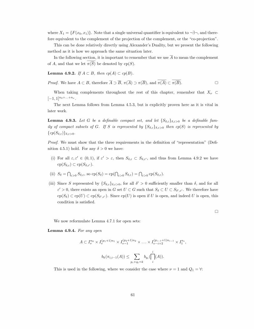
where X1 = {F (x0, x1)}. Note that a single universal quantifier is equivalent to ¬∃¬, and there­

fore equivalent to the complement of the projection of the complement, or the “co-projection”.

This can be done relatively directly using Alexander’s Duality, but we present the following

method as it is how we approach the same situation later.

In the following section, it is important to remember that we use A to mean the complement

of A, and that we let π(S) be denoted by cp(S).

Lemma 4.9.2. If A ⊂ B, then cp(A) ⊂ cp(B).

Proof. We have A ⊂ B, therefore A ⊃ B, π(A) ⊃ π(B), and π(A) ⊂ π(B).

When taking complements throughout the rest of this chapter, remember that Xν ⊂

[−1, 1]n0+...+nν .

The next Lemma follows from Lemma 4.5.3, but is explicitly proven here as it is vital in

later work.

Lemma 4.9.3. Let G be a definable compact set, and let {Sδ,ε}δ,ε>0 be a definable fam­

ily of compact subsets of G. If S is represented by {Sδ,ε}δ,ε>0 then cp(S) is represented by

{cp(Sδ,ε)}δ,ε>0.

Proof. We must show that the three requirements in the definition of “representation” (Defi­

nition 4.5.1) hold. For any δ > 0 we have:

(i) For all ε, ε� ∈ (0, 1), if ε� > ε, then Sδ,ε ⊂ Sδ,ε� , and thus from Lemma 4.9.2 we have

cp(Sδ,ε) ⊂ cp(Sδ,ε� ).

(ii) Sδ = ε>0 Sδ,ε, so cp(Sδ) = cp( ε>0 Sδ,ε) = ε>0 cp(Sδ,ε).

(iii) Since S represented by {Sδ,ε}δ,ε>0, for all δ� > 0 sufficiently smaller than δ, and for all

ε� > 0, there exists an open in G set U ⊂ G such that Sδ ⊂ U ⊂ Sδ�,ε� . We therefore have

cp(Sδ) ⊂ cp(U) ⊂ cp(Sδ�,ε� ). Since cp(U) is open if U is open, and indeed U is open, this

condition is satisfied.

We now reformulate Lemma 4.7.1 for open sets:

Lemma 4.9.4. For any open

× I(p1+1)n1 (p2+1)n2 (pi−1+1)ni−1A ⊂ In0 × Iv−1 × . . . × Iv−i+2 × Ini ,v v 1

� i

bk(πi,i−1(A)) ≤ bqi (�

(A)). pi+qi =k i

This is used in the following, where we consider the case where ν = 1 and Q1 = ∀:

61

� �

� � �

� � �

�

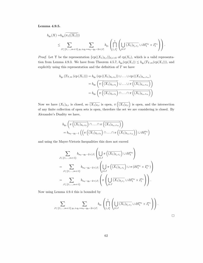
Lemma 4.9.5.

bq0 (X) =bq0 (π1((X1))) ⎛ ⎛ ⎞⎞ � � 1 ≤ bq1

⎝ � ⎝ (X1)δj ,εj ∪ ∂I1

n0 × I1 n1 ⎠⎠ .

J⊂{1,...,m+1} p1 +q1=n0−q0−2+|J| 1,J11 j∈J

Proof. Let Υ be the representation {cp((X1)δ,ε)}δ,ε>0 of cp(X1), which is a valid representa­

tion from Lemma 4.9.3. We have from Theorem 4.5.7, bq0 (cp(X1)) ≤ bq0 (TΥ,m(cp(X1))), and

explicitly using this representation and the definition of T we have

bq0 (TΥ,m (cp (X1))) = bq0 (cp ((X1)δ0,ε0 )) ∪ . . . ∪ cp ((X1)δm,εm ) � � � � ��

= bq0 π (X1)δ0,ε0 ∪ . . . ∪ π (X1)δm,εm � � � � ��

= bq0 π (X1)δ0,ε0 ∩ . . . ∩ π (X1)δm,εm

Now we have (X1)δ,ε is closed, so (X1)δ,ε is open, π (X1)δ,ε is open, and the intersection

of any finite collection of open sets is open, therefore the set we are considering is closed. By

Alexander’s Duality we have, � � � � ��

bq0 π (X1)δ0 ,ε0 ∩ . . . ∩ π (X1)δm,εm �� � � � �� � = bn0−q0−1 π (X1)δ0,ε0 ∩ . . . ∩ π (X1)δm,εm ∪ ∂I1

n0

and using the Mayer-Vietoris Inequalities this does not exceed ⎛ ⎞

bn0−q0−2+|J| ⎝ π (X1)δj ,εj ∪ ∂I1 n0 ⎠

J⊂{1,...,m+1} j∈J ⎛ ⎞

= bn0−q0−2+|J| ⎝ π (X1)δj ,εj ∪ π (∂I1 n0 × I1

n1 )⎠

J⊂{1,...,m+1} j∈J ⎛ ⎛ ⎞⎞

= bn0−q0−2+|J| ⎝π ⎝ (X1)δj εj ∪ ∂I1 n0 × I1

n1 ⎠⎠ . J⊂{1,...,m+1} j∈J

Now using Lemma 4.9.4 this is bounded by ⎛ ⎛ ⎞⎞ � � 1 bq1 ⎝

� ⎝ ∪ ∂In0 × In1 ⎠⎠ .(X1)δj ,εj 1 1 J⊂{1,...,m+1} p1 +q1 =n0−q0−2+|J| 1,J1 j∈J

1

62

� � � � �

� �

� �

�

� � �

� � � �

� �

� � �

4.9.3 Two Quantifiers ­ ∃ ∀

Lemma 4.9.6.

bq0 (X) = bq0 (π1 (cp2(X2)))

≤

1 1 p1+q1=q0 J1

1⊂J1 J22⊂J1 K1 ⊂{1,...,m} p2 +q2=t1−q1 −|J11|−|K1|−|J22|−1 ⎛ ⎛ ⎞⎞

2 1,2 ⎝ ⎝ ∪ B22⎠⎠bq2 (X2)δi,εi

2 1,J2 i∈K12

Proof. Firstly, from Lemma 4.9.1:

bq0 (X) =bq0 (π1 (cp2(X2))) ⎛ ⎞ 1⎝ ⎠bq1 (T (cp2(X2)))≤

p1+q1 =q0 1,J11

and because of Lemma 4.9.3 this is equal to ⎛ ⎞

bq1 ⎝

1�(cp2((X2)δ0,ε0 ) ∪ . . . ∪ cp2((X2)δm,εm )))⎠

1�

p1+q1=q0 1,J11 ⎛ ⎞ ⎝ ⎠bq1 π2((X2)δ0,ε0 ) ∩ . . . ∩ π2((X2)δm,εm )=

p1+q1=q0 1,J11 ⎛ ⎞

1

= bq1 ⎝ π2((X2)δ0,ε0 ) ∩ . . . ∩ π2((X2)δm,εm ) ⎠

p1+q1=q0 1,J11

which by Alexander’s Duality is bounded by ⎛ ⎞ 1 � �

bt1−q1−1 ⎝ π2((X2)δ0,ε0 ) ∩ . . . ∩ π2((X2)δm,εm ) ∪ ∂I1 t1 ⎠

p1+q1=q0 1,J11 ⎛ ⎛ ⎞ ⎞ 1

= bt1−q1 −1 ⎝ ⎝ π2((X2)δi,εi )⎠ ∪ ∂I1 t1 ⎠ .

p1+q1=q0 1,J1 0≤i≤m 1

63

� � � �

� �

� � �

� � �

� � �

� �

� �

The Mayer-Vietoris Inequalities in turn bound this by ⎛ ⎛ ⎞ ⎞ 1⎜ ⎟⎝ π2((X2)δi,εi )⎠ ∪ ∂I1

t1b t1−q1−|J11|

⎝ ⎠ ,

J11⊂J1 J1 0≤i≤m

1 p1+q1=q0 1,1

again using the Mayer-Vietoris Inequalities we have ⎛ ⎛ ⎞ ⎞ 1⎜ ⎟⎝ π2((X2)δi,εi )⎠ ∪ ∂I1

t1b ⎝ ⎠J11|t1−q1−|

1,J11 0≤i≤m ⎛ ⎞

1 J1 1≤

J2 J1 K1⊂{1,...,m}

b t1−q1−| 1 |−|K1|−|J22|−1

⎝

1,J2 i∈K1

π2((X2)δi ,εi ) ∪ ∂It1 ⎠

12 ⊂ ⎛ 2 ⎞

1

�

2�

= b t1−q1−|J11|−|K1|−|J22|−1

⎝ π2((X2)δi ,εi ) ∪ π2,1(∂I1 t1 × I1

n2 )⎠

J22⊂J11 K1⊂{1,...,m} 1,J2

2 i∈K1 ⎛ ⎛ ⎞⎞ 1,2

= b t1−q1−|J11|−|K1|−|J22|−1

⎝π2,1 ⎝ (X2)δi ,εi ∪ ∂I1 t1 × I1

n2 ⎠⎠

J22⊂J1 K1⊂{1,...,m} 1,J2 i∈K1

1 2

and by Lemma 4.7.1 we have ⎛ ⎛ ⎞⎞ 1,2

J1 1 1b t1−q1−| 1 |−|K1|−|J22|−1

⎝π2,1 ⎝ (X2)δi,εi ∪ ∂It1 × In2 ⎠⎠

1,J2 i∈K12 ⎛ ⎛ ⎞⎞ 1,2 ⎝ ⎝ (X2)δi ,εi ∪ ∂I1

t1 × I1 n2 ⎠⎠bq2≤

2�

2p2+q2 =t1−q1−|J11|−|K1|−|J22 |−1 ⎛ 2 ⎛

1,J2 i∈K1 ⎞⎞ 1,2 ⎝ ⎝ ∪ B2

2⎠⎠bq2 (X2)δi ,εi =

2p2+q2=t1−q1−|J11|−|K1|−|J22 |−1 2 1,J2 i∈K1

64

� � � � �

� � �

�

� � � �

� �

� �

� �

� �

� �

� �

4.9.4 Three Quantifiers ­ ∃ ∀ ∃

Lemma 4.9.7.

bq0 (X) =bq0 (π1 (cp2(π3(X3))))

≤

1 1 p1+q1=q0 J1

1⊂J1 J22⊂J1 K1⊂{1,...,m} p2+q2=t1−q1−|J11 |−|K1|−|J22|−1

1≤k2≤p2+1 J�22⊂{1,...,p2+1},|J�22|=k2 1≤s2≤q2+k2+1+|K1 |

J21⊂J1 J�2,J22⊂J2 J�2,K2⊂K1,|J21|+|J22|+|K1|=s22 21 × 1 × ⎛ ⎛ � � ⎞⎞

3 1,3 2,3 B3

2 ∪ B33⎝ ⎝ ⎠⎠bq3 (X3)δi,εi ∪

p3+q3=t2−q2−k2+s2−1 3 2,J1 i∈K2 2,J2 2 2

where J1 = {1, . . . , p1 + 1}.1

Proof. Working from the results in the previous section, we have a summand involving ⎛ ⎛ ⎞⎞ 2 1,2 ⎝ ⎝ (X2)δi,εi ∪ B2

2⎠⎠bq2 . 2 1,J2 i∈K12

From De Morgan’s Law and Alexander’s duality, this is equal to

1 2,� ⎛ ⎛ ⎞⎞

2⎜ ⎟⎝ ∩ B22⎠bq2 (X2)δi ,εi⎝ ⎠

1 2,�

2 1,J2 i∈K12 ⎛ ⎛ ⎞ ⎞ 2 ⎠ n2(p2+1)⎝ ⎝ ⎠∪ ∂(It2

2∩ B22= bt2−q2−1 (X2)δi ,εi × I ) .1

1 22 ,�

2 1,J22 i∈K1

By the Mayer-Vietoris inequality the preceding is bounded by

1≤k2≤p2+1 J�22⊂{1,...,p2+1},|J�22|=k2 ⎛ ⎛ ⎞ ⎞ ⎠ n2 (p2+1)⎝ ⎝ ⎠∪ ∂(It2 2∩ B2

2bt2−q2−k2 (X2)δi,εi × I ) ,1

1 2�

2,J�22 1,J22 i∈K1

with the summand of this expression being equal to ⎛ � � ⎞

n2(p2+1)⎝ ⎠B22 ∪ ∂(It2

2bt2−q2−k2 (X2)δi,εi × I )∩ ,1

2,J11 ×J�2 i∈K1 2,J1

2 ×J�2 2 2

65

� �

�

� �

� �

� � �

with J12 = {1}. By the Mayer-Vietoris inequality, this is bounded by

1≤s2≤q2+k2+1+|K1 | J21⊂J11 ×J�22,J22⊂J12 ×J�22,K2⊂K1,|J21|+|J22|+|K1|=s2 ⎛ � � ⎞ � 1 2

bt2 −q2−k2+s2 −1 ⎝ (X2)δi,εi ∪ B22 ∪ ∂(I2

t2 × I1 n2(p2+1)

)⎠ , 2,J2

1 i∈K2 2,J2 2

We have X2 = π3(X3), and π3(X3) is represented by π3((X3)δ,ε), so the summand of the

previous expression is equal to ⎛ � � ⎞ 1 2

bt2−q2−k2 +s2−1 ⎝ π3((X3)δi,εi ) ∪ π3,1(B32) ∪ π3,2(∂(I2

t2 × I1 n2 (p2+1)

) × I1 n3 )⎠

2,J21 i∈K2 2,J2

2

which is equal to ⎛ ⎛ � � ⎞⎞ 1,3 2,3

bt2−q2−k2+s2−1 ⎝π3,2 ⎝ (X3)δi,εi ∪ B32 ∪ B3

3⎠⎠ , 2,J1 i∈K2 2,J2

2 2

which in turn is bounded by ⎛ ⎛ � � ⎞⎞ 3 1,3 2,3

bq3 ⎝� ⎝ (X3)δi,εi ∪ B3

2 ∪ B33⎠⎠ ,

p3+q3 =t2−q2−k2+s2−1 3 2,J1 i∈K2 2,J2 2 2

4.9.5 Arbitrary number of Quantifiers

In the following, we take Q1 = ∃. The other case can be computed similarly, or calculated

directly using Alexander’s duality. We follow the general idea used in the two and three

quantifier cases, and proceed using induction.

Theorem 4.9.8 (Main Result A). For any i, let τi = πi if i is odd and τi = cpi if i is even.

66

���� � � � �

� � �

� � �

� � �

�

�

� � �

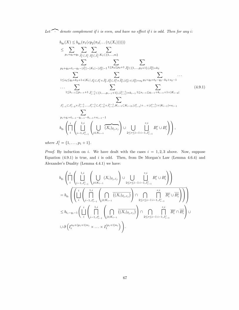
Let denote complement if i is even, and have no effect if i is odd. Then for any i:·

bq0 (X) ≤ bq0 (π1(cp2(π3(. . . (τi(Xi))))))

≤ p1+q1 =q0 J1

1⊂J1 J22⊂J1 K1⊂{1,...,m}

1 1

p2+q2 =t1−q1−|J11|−|K1 |−|J22|−1 1≤k2≤p2+1 J22⊂{1,...,p2+1},|J22|=k2

. . . 1≤s2≤q2 +k2+1+|K1| J21⊂J11 ×J2,J2

2⊂J12 ×J22 ,|J21|+|J22|=s2 p3+q3 =t2−q2−k2+s2−1 2

. . . (4.9.1) 1≤ki−1≤pi−1+1 Ji−1 Ji−1 1≤si−1≤qi−1 +ki−1+1+|Ki−2|

i−1 ⊂{1,...,pi−1+1},| ˆi−1 |=ki−1

J1 Ji−1,...,Jii−−11 ⊂Ji−1 Ji−1,Ki−1⊂Ki−2,|Ji1

−1|+...+|Ji−1 i−1⊂Ji1

−2 × i−1 i−2 × i−1 i−1 |+|Ki−1|=si−1

pi+qi=ti−1−qi−1−ki−1 +si−1−1 ⎛ ⎛ ⎛ ⎞ ⎞⎞ i 1,i r,i⎝� ⎝ � ⎝ � �� �⎠

� Br ⎠⎠ ,bqi (Xi)δj ,εj ∪ i ∪ Bi

i

i i−1,Ji1 −1

j∈Ki−1 2≤r≤i−1 i−1,Jir −1

where J1 = {1, . . . , p1 + 1}.1

Proof. By induction on i. We have dealt with the cases i = 1, 2, 3 above. Now, suppose

Equation (4.9.1) is true, and i is odd. Then, from De Morgan’s Law (Lemma 4.6.4) and

Alexander’s Duality (Lemma 4.4.1) we have: ⎛ ⎛ ⎛ ⎞ ⎞⎞ i 1,i r,i

bqi ⎝� ⎝

� ⎝ (Xi)δj ,εj

⎠ ∪ �

Br ∪ Bi⎠⎠i i

i i−1,Ji1 −1

j∈Ki−1 2≤r≤i−1 i−1,Jir −1 ⎛⎛ ⎛ ⎛ ⎞ ⎞⎞⎞

i 1,i r,i⎜⎝� ⎝ � ⎝ � � �⎠ � �

Br ⎠⎠⎟ = bqi ⎝ (Xi)δj ,εj ∩ ∪ Bi ⎠i i

i i−1,Ji1 −1

j∈Ki−1 2≤r≤i−1 i−1,Jir −1 � ⎛ ⎛ ⎞ ⎞

i 1,i r,i

≤ bti−qi−1

� ⎝ � ⎝ � �

(Xi)δj ,εj

�⎠ ∩ � �

Bir ∩ Bi

i⎠ ∪ i i−1,Ji

1 −1

j∈Ki−1 2≤r≤i−1 i−1,Jir −1

∪ ∂ Iin0+(p1+1)n1 × . . . × I(pi+1)ni .1

67

� ��

� �

� � � �

� ��

Using the Mayer-Vietoris Inequality (Lemma 1.5.23), this is bounded by ⎛ ⎛ ⎛ ⎞ � � i 1,i � � � ⎝ � ⎝

� ⎝ ⎠bti−qi−ki (Xi)δj ,εj ∩ 1≤ki≤pi+1 Ji

i⊂{1,...,pi+1},|Jii|=ki i,Jii i−1,Ji

1 −1

j∈Ki−1 ⎞ ⎞ � r,i � � n0+(p1 +1)n1 (pi+1)ni∩

� Bir ∩ Bi

i⎠ ∪ ∂ Ii × . . . × I1 ⎠ ,

2≤r≤i−1 i−1,Jir −1

and, by Lemma 4.6.2, the summand is bounded by ⎛ ⎛ ⎞ 1 r⎜ � ⎝ � � �⎠ � �

Brbti−qi−ki ⎝ (Xi)δj ,εj ∩ i ∪ i,Ji

1 −1 ×Ji j∈Ki−1 2≤r≤i i,Jir

−1×Ji i i

∪∂ Iin0+(p1 +1)n1 × . . . × I1

(pi+1)ni ,

where Jii −1 = {1}. Using the Mayer-Vietoris Inequality (Lemma 1.5.23), the last expression

does not exceed

1≤si≤qi+ki+1+|Ki−1 | Ji 1⊂Ji1

−1×Jii,...,Jii⊂Jii −1×Ji,Ki⊂Ki−1,|Ji

1|+...+|Jii|+|Ki|=sii ⎛ ⎛ ⎞ 1 r

bti−qi−ki+si −1 ⎝ ⎝ (Xi)δj ,εj ⎠ ∪ Bi

r

i,J1 j∈Ki 2≤r≤i i,Jiri

∪ ∂ Iin0 +(p1+1)n1 × . . . × I1

(pi+1)ni .

We have Xi = cpi+1(Xi+1), and by Lemma 4.9.3 cpi+1(Xi+1) is represented by cp((Xi+1)δ,ε),

68

� � � � �

� � �

� � �

�

�

� � � �

� � �

�

so the summand of the previous expression is equal to ⎛ ⎛ ⎞ 1

bti−qi−ki+si−1 ⎝ ⎝ cpi+1((Xi+1)δj ,εj ) ⎠ ∪ i,J1 j∈Kii ⎞ r �

Bir ∪ ∂ Ii

n0+(p1+1)n1 × . . . × I(pi+1)ni ⎠1

2≤r≤i i,Jri ⎛ ⎛ ⎞

1

= bti−qi−ki+si−1 ⎝ ⎝ πi+1((Xi+1)δj ,εj ) ⎠ ∪i,Ji

1 j∈Ki ⎞ r

Bir ∪ ∂ Ii

n0+(p1+1)n1 × . . . × I1(pi+1)ni ⎠

2≤r≤i i,Jir ⎛ 1 � �

= bti−qi−ki+si−1 ⎝ πi+1((Xi+1)δj ,εj ) ∪i,J1 j∈Kii ⎞

r � � � � πi+1,r−1(Bi

r +1) ∪ πi+1,i ∂ I

n0+(p1+1)n1 × . . . × I(pi+1)ni × Ini+1 ⎠ ,i 1 1 2≤r≤i i,Jr

i

and bringing the projection to the front, this is equal to ⎛ ⎛ ⎞⎞ 1,i+1 r,i+1⎝ Bi

r +1 ∪ Bi+1⎠⎠ .bti−qi−ki+si−1 ⎝πi+1,i (Xi+1)δj ,εj ∪ i+1

i,Ji 1 j∈Ki 2≤r≤i i,Jir

Finally, from Lemma 4.7.1, this is bounded by ⎛ ⎛ ⎞⎞ i+1 1,i+1 � � r,i+1⎝� ⎝ (Xi+1)δj ,εj Bi

r +1 ∪ Bi+1⎠⎠ .bqi+1 ∪ i+1

pi+1+qi+1 =ti−qi−ki+si −1 i+1 i,J1 j∈Ki 2≤r≤i i,Jiri � �

The case when i is even follows directly by replacing j∈Ki−1 (Xi)δj ,εj with j∈Ki−1

(Xi)δj ,εj

at the start of the proof, immediately changing to

(Xi)δj ,εj

j∈Ki−1

in the next line and carrying this through to the stage where projections are introduced, re­� � placing j∈Ki

(Xi)δj ,εj with j∈Ki πi+1((Xi+1)δj ,εj ), and finishing with an expression involving �

j∈Ki (Xi+1)δj ,εj .

69

� � � �

� � �

� � �

�

�

� �

� �

4.10 Upper Bounds

We have succeeded in finding an expression to bound each Betti number of X, in terms of some

quantifier-free formula involving a set we can bound using the tools in the above chapters.

It now remains to explicitly deduce a formula using the functions supplied by the complexity

definition.

Theorem 4.9.8 tells us that bq0 (X) is bounded by:

p1 +q1 =q0 J11 ⊂J1 J2

2 ⊂J1 K1⊂{1,...,m}1 1

p2+q2 =t1−q1−|J11|−|K1|−|J22|−1 1≤k2 ≤p2+1 J22⊂{1,...,p2+1},|J22|=k2

. . . 1≤s2≤q2+k2+1+|K1| J21⊂J1 J2,J2

2 ⊂J2 J22 ,|J21|+|J22|=s2 p3 +q3 =t2−q2 −k2+s2−1 �

1 × � 1 × �

2

. . . Ji−1 Ji−11≤ki−1≤pi−1+1 ˆi−1 ⊂{1,...,pi−1+1},| ˆi−1 |=ki−1 1≤si−1≤qi−1+ki−1+1+|Ki−2|

J1 Ji−1,...,Ji−1 Ji−1,Ki−1⊂Ki−2 ,|Ji1 −1|+...+|Ji−1

i−1⊂J1 i−1 ⊂J

i−1 i−1 |+|Ki−1|=si−1i−2× i−1 i−2 × i−1

pi+qi=ti−1−qi−1−ki−1+si−1−1 ⎛ ⎛ ⎛ ⎞ ⎞⎞ i 1,i � �� � r,i

bqi ⎝� ⎝

� ⎝ (Xi)δj ,εj

⎠ ∪ �

Bir ∪ Bi

i⎠⎠ . i i−1,Ji

1 −1

j∈Ki−1 2≤r≤i−1 i−1,Jir −1

We start by bounding the Betti numbers of the summand. To do this we prove the following

lemma, which allows us to use the results in the previous sections.

Lemma 4.10.1. Let Xν be defined by a quantifier-free Boolean formula, consisting of s atoms

of the type fi > 0 or fi = 0. Let tν be defined as in Definition 4.6.5. Then the set ⎛ ⎛ ⎞ ⎞ ν 1,ν r,ν� ⎝

� ⎝ (� Xν

�� )δj ,ε

� j ⎠ ∪

� Bνr ∪ Bν

ν ⎠ ⊂ Rtν

ν ν−1,Jν1 −1

j∈Kν−1 2≤r≤ν−1 ν−1,Jνr −1

is defined by a quantifier-free Boolean formula with no negations, having at most

(2tν−2 + 1) 4s (n0 + . . . + nν ) + 2tν−1 + 2nν + (4tr−1 + 2 (nr + . . . + nν ))·

(2tν−2 + 1) + 2tν−1 + 2nν (ν − 2) (tν−1 + 1) ≤ st O(1) · ν−1

atoms.

Proof. Our method consists of simple counting and calculation.

70

� �� �

� �� �

�

• The set (Xν )δj ,εj is defined by a Boolean formula with no negations consisting of 4s

non-strict inequalities of the type f + δj , f − δj , f + εj , and f − εj .

• The set (Xν )δj ,εj is either the same as the above, or its negation, which is a Boolean

formula with no negations consisting of 4s strict inequalities. Either way, the set is

defined by only non-strict or only strict inequalities, and no negations.

• We have {1, . . . ,m} ⊃ K1 ⊃ . . . ⊃ Kν , so |Ki| ≤ m for all i. We define m when

constructing T , and from Theorem 4.5.7 we know if m is at least the dimension of the

space, then T is a ‘good’ approximation. The maximum dimension we work in is n0 +

. . . + nν . Therefore

(Xν )δj ,εj

j∈Kν−1

is a set defined by a Boolean formula with no negations consisting of at most 4s(n0 +

. . . + nν ) only strict or only non-strict inequalities.

• The set ⎛ ⎞ 1,ν � �� � ⎝ (Xν )δj ,εj

⎠ ⊂ Rtν−1+nν

ν−1,Jν1 −1

j∈Kν−1

is defined by a Boolean formula with no negations having |Jν1 −1|4s(n0 + . . . + nν ) ≤

sν−14s(n0 + . . . + nν ) ≤ (2tν−2 + 1)4s(n0 + . . . + nν ) atoms, and at most 2tν−1 + 2nν

linear atoms (defining I1 tν−1 +nν ).

• For any 2 ≤ r ≤ ν, the set Bνν ⊂ Rtr−1 +nr is defined by a Boolean formula with no

negations having 4tr−1 + 2nr linear atomic inequalities.

• Therefore, all sets of the kind Bjr for j ≥ r are defined by Boolean formulae with no

negations having 4tr−1 + 2(nr + . . . + nj ) linear inequalities. In particular the set Bνr ⊂

Rtr−1 +nr +...+nν is defined by 4tr−1 + 2(nr + . . . + nν ) linear atomic inequalities. ��r,ν • For any 2 ≤ r ≤ ν − 1, the set ν−1,Jνr −1 Bνr ⊂ Rtν−1 +nν is defined by a formula with no

negations having at most

(4tr−1 + 2(nr + . . . + nν ))|Jνr −1| + 2tν−1 + 2nν

≤(4tr−1 + 2(nr + . . . + nν ))sν−1 + 2tν−1 + 2nν

≤(4tr−1 + 2(nr + . . . + nν ))(2tν−2 + 1) + 2tν−1 + 2nν

linear atoms. � ��r,ν • The set 2≤r≤ν−1 ν−1,Jνr −1 Bνr ⊂ Rtν−1+nν is therefore defined by a Boolean formula

with no negations having at most

((4tr−1 + 2(nr + . . . + nν ))(2tν−2 + 1) + 2tν−1 + 2nν )(ν − 2)

71

� �

� �

� � �

� �

atoms.

• Therefore, the set ⎛ ⎛ ⎞ ⎞ ν � � �� � � � ⎝

1,ν ⎝ (Xν )δj ,εj ⎠ ∪

r,ν

Bνr ∪ Bν ⎠

ν ν ν−1,Jν

1 −1

j∈Kν−1 2≤r≤ν−1 ν−1,Jνr −1

is defined by a Boolean formula with no negations having at most

(2tν−2 + 1) 4s (n0 + . . . + nν ) + 2tν−1 + 2nν + (4tr−1 + 2 (nr + . . . + nν ))·

(2tν−2 + 1) + 2tν−1 + 2nν (ν − 2) (tν−1 + 1) ≤ st O(1) · ν−1

atoms.

We can now use Corollary 3.4.14, along with our particular defined complexity, to find an

upper bound for ⎛ ⎛ ⎞ ⎞ ν 1,ν r,ν� ⎝

� ⎝ (� Xν

�� )δj ,ε

� j ⎠

� Bνr ∪ Bν

ν ⎠ .∪ ν ν−1,Jν

1 −1

j∈Kν−1 2≤r≤ν−1 ν−1,Jνr −1

We now count the number of times this expression is added. We use the following notation,

taken from [11]:

Definition 4.10.2. Let f, g, h : Nl → N be three functions. The expression f ≤ gO(h) means

that there exists c ∈ N such that f ≤ gch everywhere on Nl .

Lemma 4.10.3. The number of additive terms in (4.9.8) does not exceed

2O(i2 (2(n0+...+nν ))i n0n1...ni−2 ).

Proof. Firstly, we have to count the number of terms introduced by

.

J11⊂J1 J2

2⊂J1 K1⊂{1,...,m}1 1

We have J1 = {1, . . . , p1 + 1}, so the number of terms in the first summation is bounded by 1

2p1+1 , as is that in the second summation, and the third summation has no more than 2m

terms.

Next we can partition the remaining terms into i − 1 groups of the kind

1≤kj ≤pj +1 Jjj ⊂{1,...,pj +1},|Jj

j |=kj

72

�

�

�

�

�

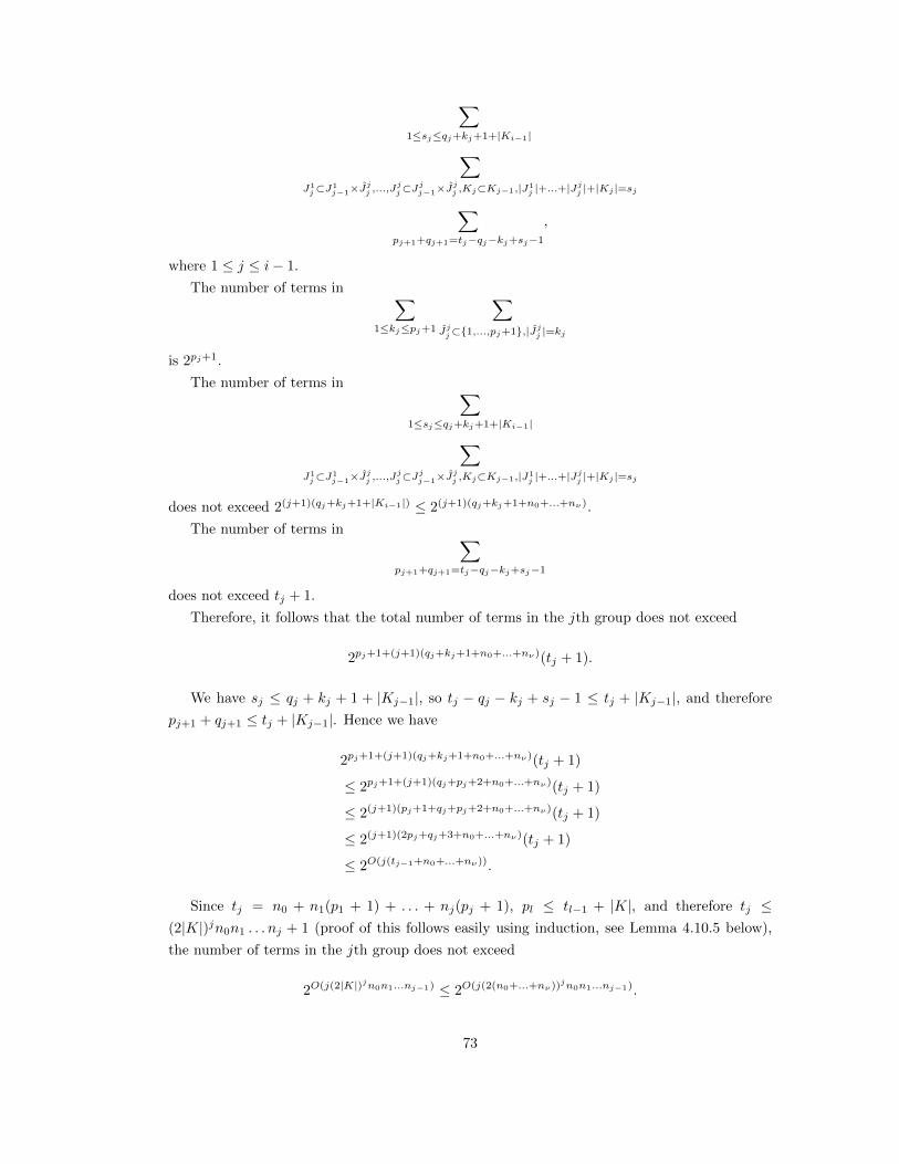
1≤sj ≤qj +kj +1+|Ki−1 |

Jj 1 ⊂J1 Jj ,...,Jj j Jj j

j−1× j j ⊂Jj−1× ,Kj ⊂Kj−1,|J1 j |+...+|Jj |+|Kj |=sjj � ,

pj+1+qj+1=tj −qj −kj +sj −1

where 1 ≤ j ≤ i − 1.

The number of terms in � �

1≤kj ≤pj +1 Jjj ⊂{1,...,pj +1},|Jj

j |=kj

is 2pj +1 .

The number of terms in

1≤sj ≤qj +kj +1+|Ki−1|

Jj 1 ⊂Jj1

−1×Jj ,...,Jj

j ⊂Jjj −1×Jj

j ,Kj ⊂Kj−1,|Jj 1|+...+|Jj

j |+|Kj |=sjj

does not exceed 2(j+1)(qj +kj +1+|Ki−1|) ≤ 2(j+1)(qj +kj +1+n0+...+nν ).

The number of terms in

pj+1+qj+1 =tj −qj −kj +sj −1

does not exceed tj + 1.

Therefore, it follows that the total number of terms in the jth group does not exceed

2pj +1+(j+1)(qj +kj +1+n0+...+nν )(tj + 1).

We have sj ≤ qj + kj + 1 + |Kj−1|, so tj − qj − kj + sj − 1 ≤ tj + |Kj−1|, and therefore

pj+1 + qj+1 ≤ tj + |Kj−1|. Hence we have

2pj +1+(j+1)(qj +kj +1+n0+...+nν )(tj + 1)

≤ 2pj +1+(j+1)(qj +pj +2+n0+...+nν )(tj + 1)

≤ 2(j+1)(pj +1+qj +pj +2+n0+...+nν )(tj + 1)

≤ 2(j+1)(2pj +qj +3+n0+...+nν )(tj + 1)

≤ 2O(j(tj−1 +n0+...+nν )).

Since tj = n0 + n1(p1 + 1) + . . . + nj (pj + 1), pl ≤ tl−1 + |K|, and therefore tj ≤

(2|K|)j n0n1 . . . nj + 1 (proof of this follows easily using induction, see Lemma 4.10.5 below),

the number of terms in the jth group does not exceed

2O(j(2|K|)j n0n1 ...nj−1) ≤ 2O(j(2(n0+...+nν ))j n0n1...nj−1).

73

� �

�

It follows that the total number of terms in (4.9.8) does not exceed

2O(i2 (2(n0+...+nν ))i n0n1...ni−2 ).

Remark 4.10.4. Thanks to James Davenport for suggesting this improvement during the viva.

In the preceding we counted each of the Σ separately, for example for

J11⊂J11 J2

2⊂J11

we bounded each of the summations by 2p1+1 and get a total of 4p1+1 . We could, however

rewrite this as

J22⊂J11⊂J1

1

and bound this by 3p1+1, resulting in a slightly better bound. Similar techniques could be used

throughout. This does not produce any difference at the level of 2O(...), but may be useful in

future work.

Lemma 4.10.5.

tj ≤ (2|K|)j n0n1 . . . nj + 1

Proof. By induction. Firstly, we have tj = n0 + n1(p1 +1)+ . . .+nj (pj +1) and pl ≤ tl−1 + |K|.

• For j = 0, t0 = n0

• For j = 1,

– If n0 > 1 or n1 > 1

t1 = n0 + n1(p1 + 1)

≤ n0 + n1(n0 + |K| + 1)

= n0 + n1 + n0n1 + n1|K|

≤ 2n0n1 + n1|K|, since n0 and n1 are positive integers and not both 1

≤ 2|K|n0n1, as |K| ≥ 2

– If n0 = n1 = 1 we have

t1 = n0 + n1(p1 + 1)

≤ 1 + 1(1 + |K| + 1)

= |K| + 3 and as |K| ≥ 2

≤ 2|K| + 1

74

� �

• Assume tj ≤ (2|K|)j n0n1 . . . nj . Then

tj+1 = tj + nj+1(pj+1 + 1)

≤ tj + nj+1(tj + |K| + 1)

≤ (2|K|)j n0n1 . . . nj + (2|K|)j n0n1 . . . nj nj+1 + nj+1|K| + nj+1

≤ 2j+1 j|K| n0n1 . . . nj nj+1 + nj+1|K|

≤ (2|K|)j+1 n0n1 . . . nj nj+1

We now know how to calculate the Betti numbers of the summand, and we know how many

times we are summing, so we only need to use a result from the previous sections to produce a

concrete bound.

We will use Corollary 3.4.14, (which is equivalent to the bound O(s2d)n in the basic poly­

nomial, degree case).

Definition 4.10.6. For a set of functions F = {f1, . . . , fs} from H R, where H ⊂ Rn define→

the function

Ω(F ) = max γ(n, c(fi

2 + |x|2)) .

1≤i≤s 2

Note the following is really a Corollary of Theorem 4.9.8, but is called a Theorem because

it is one of the most significant results of this thesis.

Theorem 4.10.7 (Main Result B). Let C denote the maximum complexity of the atoms in ⎛ ⎛ ⎞ ⎞ ν 1,ν r,ν

Z = � ⎝

� ⎝ (� Xν

�� )δj ,ε

� j ⎠ ∪

� Bνr ∪ Bν ⎠ .ν

ν ν−1,Jν1 −1

j∈Kν−1 2≤r≤ν−1 ν−1,Jνr −1

Let F be a set containing elements g, |x|2, where g is any function of complexity C with domain

Rtν . Let uj = n0 + n1 + . . . + nj , and wj = n0n1 . . . nj . Then:

νbq0 (X) ≤ (2ν2

uν swν−1)O((2uν )

ν wν )Ω(F ).

Proof. We take Theorem 4.9.8 in the case i = ν. Firstly, we directly apply the bound given in

3.4.14 to the set Z ⊂ Rtν , which is defined by st O(1) atoms, and get ν−1

bq0 (Z) ≤ O((st O(1))2tν Ω(F ))ν−1

From Lemma 4.10.3 we know that we are adding this together

2O(ν2 (2(n0+...+nν ))ν n0n1...nν−2)

75

times, so we have

(X) ≤ 2O(ν2(2(n0+...+nν ))ν n0 n1...nν−2)O((st O(1)

bq0 ν−1 )2tν Ω(F ))

≤ 2O(ν2(2(n0+...+nν ))ν n0 n1...nν−2)O((stν−1)

O(tν )Ω(F ))

We have tj ≤ (2|K|)j n0n1 . . . nj ≤ (2(n0 + . . . + nν ))j n0n1 . . . nj , so

bq0 (X) ≤ 2O(ν2(2(n0+...+nν ))ν n0n1...nν−2) ·

O((s(2(n0 + . . . + nν ))ν−1 n0n1 . . . nν−1)

O((2(n0+...+nν ))ν n0 n1...nν )Ω(F ))·

And substituting uj = n0 + n1 + . . . + nj , wj = n0n1 . . . nj gives

bq0 (X) ≤ 2O(ν2 (2uν )ν wν−2)O((s(2uν )

ν−1 wν−1)O((2uν )

ν wν )Ω(F )) ν≤ (2ν

2

uν swν−1)O((2uν )

ν wν )Ω(F ).

In the preceding result, and the following examples, we see a uνν factor appearing in a number

of places. This is the consequence of not restricting to the case of Xν being open or closed,

and thus needing to use the T construction to approximate by a compact set. To construct T

we take the union of m sets, and we use n0 + . . . + nν = uν to bound m, which results in this

extra factor. A possible improvement would be to find a tighter bound for m.

Example 4.10.8 (The Degree of a Polynomial). If the original polynomials have maximum

degree d, then the polynomials defining Z will also have maximum degree d, and Ω(F ) =

O(dtν ) ≤ O(d(2(n0+...+nν ))ν n0 n1...nν ), so

ν wν )bq0 (X) ≤ (2ν2

uν dswν−1)O((2uν )

ν

.

Note the difference to the bound of

wν )(2ν2

dswν−1)O(2ν

.

in section 8.1 of [12] for the case where Xν is open or closed.

Example 4.10.9 (Pfaffian Functions). If the functions defining Xν are Pfaffian functions of

order r, degree (α, β), then the functions defining Z are Pfaffian functions of degree (α, β) and

76

order at most r(2tν−2 + 1)(tν−1 + 1) = O(rtν−2tν−1). We then have

Ω(F ) =2O(rtν−2 tν−1 )(O(rtν−2tν−1)−1)/2β(α + 2β − 1)tν −1 ·

(min{tν , O(rtν−2tν−1)}α + 2tν β + (tν − 1)α − 2tν + 2)O(rtν−2tν−1) ·

≤2O(rtν−2 tν−1 )2

β(α + 2β − 1)tν −1 ·

(min{tν , O(rtν−2tν−1)}α + 2tν β + (tν − 1)α − 2tν + 2)O(rtν−2tν−1) ·

≤2O(rtν−2 tν−1 )2

(α + β)O(tν ) ·

(min{tν , O(rtν−2tν−1)}α + 2tν β + (tν − 1)α − 2tν + 2)O(rtν−2tν−1) ·

≤2O(rtν−2 tν−1 )2

(α + β)O(tν )(tν (α + β))O(rtν−2tν−1).

We have tj ≤ (2(n0 + . . . + nν ))j n0n1 . . . nj = (2uν )

j wj , so

Ω(F ) ≤2O(r(2uν )ν−2 wν−2(2uν )

ν−1 wν−1)2

(α + β)O((2uν )ν wν )

((2uν )ν wν (α + β))O(r(2uν )

ν−2 wν−2(2uν )ν−1 wν−1 )

≤2O(r 2(2uν )4ν wν

2 −2wν

2 −1)(α + β)O((2uν )

ν wν )((2uν )ν wν (α + β))O(r(2uν )

2ν wν−2 wν−1 ).

Now we have

bq0 (X) ≤(2ν2

u νν swν−1)O((2uν )

ν wν )2O(r 2(2uν )4ν wν

2 −2wν

2 −1)(α + β)O((2uν )

ν wν )

((2uν )ν wν (α + β))O(r(2uν )

2ν wν−2wν−1 )

2 2 2O((2uν )ν wν )(w O((2uν )

ν wν ))(2ν2

uνν )O((2uν )

ν wν )2O(r (2uν )4ν wν−2 wν−1)(α + β)O((2uν )

ν wν )≤s ν−1

((2uν )ν wν (α + β))O(r(2uν )

2ν wν−2wν−1 )

≤s O((2uν )ν wν )(2ν

2

u νν )O((2uν )

ν wν )2O(r 2(2uν )4ν w 2 2 )(wν−1(α + β))O((2uν )

ν wν )ν−2wν−1

((2uν )ν wν (α + β))O(r(2uν )

2ν wν−2wν−1 )

≤s O((2uν )ν wν )(2ν

2

uνν )O((2uν )

ν wν )2O(r 2(2uν )4ν wν

2 −2wν

2 −1)((2uν )

ν )O(r(2uν )2ν wν−2wν−1)

(wν (α + β))O((2uν )ν wν +r(2uν )

2ν wν−2wν−1 )

≤s O((2uν )ν wν )(2ν

2

u νν )O((2uν )

ν wν )2O(r 2(2uν )4ν wν

2 −2wν

2 −1)((2uν )

ν )O(r(2uν )2ν wν−2wν−1)

(wν (α + β))O((2uν )ν wν +r(2uν )

2ν wν−2wν−1 )

≤s O((2uν )ν wν )(2ν

2

uνν )O((2uν )

ν wν )(2uν )O(ν(r(2uν )

2ν wν−2wν−1)+r 2(2uν )4ν wν

2 −2wν

2 −1)

(wν (α + β))O((2uν )ν wν +r(2uν )

2ν wν−2wν−1 )

≤s O((2uν )ν wν )(2ν

2

u νν )O((2uν )

ν wν )(2uν )O(r 2 (2uν )

4ν wν2 −2wν

2 −1)

(wν (α + β))O((2uν )ν wν +r(2uν )

2ν wν−2wν−1 )

≤s O((2uν )ν wν )(2ν uν )

O(ν(2uν )ν wν +r 2(2uν )

4ν wν2 −2wν

2 −1 )

(wν (α + β))O((2uν )ν wν +r(2uν )

2ν wν−2wν−1 ).

77

Compare this with the bound of

s O(2ν wν )2O(ν2ν wν +r 224ν wν2 −2wν

2 −1 )(wν (α + β))O(2ν wν +r2

2ν wν−2wν−1)

given in section 8.2 of [12] for the case where Xν is open or closed.

78

79

Bibliography

[1] Saugata Basu. On bounding the Betti numbers and computing the Euler characteristic of

semi-algebraic sets. Discrete and Computational Geometry, 22:1–18, 1999.

[2] Saugata Basu, Richard Pollack, and Marie-Francoise Roy. Algorithms in Real Algebraic

Geometry. Algorithms and Computations in Mathematics. Springer, Berlin, 2003.

[3] Saugata Basu, Richard Pollack, and Marie-Francoise Roy. On the Betti numbers of sign

conditions. Proceedings of the American Mathematical Society, 133(4):965–974, 2005.

[4] Riccardo Benedetti and Jean-Jacques Risler. Real Algebraic and Semi-Algebraic Sets.

Hermann, Editurs Des Sciences Et Des Arts, Paris, 1990.

[5] Timothy Chow. You could have invented spectral sequences. Notices of the American

Mathematical Society, 53:15–19, 2006.

[6] Michel Coste. An Introduction to O-Minimal Geometry. RAAG publications, November

1999.

[7] Michel Coste. An Introduction to Semi-Algebraic Geometry. RAAG publications, October

2002.

[8] Andrei Gabrielov. Counterexamples to quantifier elimination for fewnomial and exponen­

tial expressions. Moscow Mathematical Journal, 7:453–460, 2007.

[9] Andrei Gabrielov and Nicolai Vorobjov. Complexity of computations with Pfaffian and

Noetherian functions. Normal Forms, Bifurcations and Finiteness Problems in Differential

Equations, pages 211–250, 2004.

[10] Andrei Gabrielov and Nicolai Vorobjov. Betti numbers of semialgebraic sets defined by

quantifier-free formulae. Discrete and Computational Geometry, 33:395–401, 2005.

[11] Andrei Gabrielov and Nicolai Vorobjov. Approximation of definable sets by compact

families, and upper bounds on homotopy and homology. J. London Math. Soc., 80(1):35–

54, 2009.

[12] Andrei Gabrielov, Nicolai Vorobjov, and Thierry Zell. Betti numbers of semialgebraic and

sub-Pfaffian sets. Journal of the London Mathematical Society, 69:27–43, 2004.

80

[13] Allen Hatcher. Algebraic Topology. Cambridge University Press, 2002.

[14] Morris Hirsch. Differential Topology. Graduate Texts in Mathematics. Springer-Verlag,

New York, 1976.

[15] Askold Khovanskii. On a class system of transcendental equations. Soviet Math. Dokl.,

(22):762–765, 1980.

[16] Askold Khovanskii. Fewnomials. Transl. Math. Monogr., (88), 1991. Amer. Math. Soc.,

Providence, RI.

[17] John Milnor. On the Betti numbers of real varieties. Proc. AMS, 15:275–280, 1964.

[18] Olga Oleinik and Ivan Petrovsky. On the topology of real algebraic surfaces. Izvestiia

Akademii Nauk Sssr Seriia Matematicheskaia, 13:389–402, 1949.

[19] Rene Thom. Sur l’homologie des varits algebriques relles. In Differential and Combinatorial

Topology, pages 255–265. Princeton University Press, Princeton, 1965.

[20] Lou van den Dries. Tame topoplogy and O-Minimal Structures. Cambridge University

Press, 1998.

[21] Alex Wilkie. A theorem of the complement and some new o-minimal structures. Selecta

Mathematica, New Series, 5:397–421, 1999. 10.1007/s000290050052.

[22] Thierry Zell. Betti numbers of semi-Pfaffian sets. Journal of Pure and Applied Algebra,

pages 323–338, 1999.

81